analytic number theory in function fields (lecture...
TRANSCRIPT
Analytic Number Theory in Function Fields(Lecture 1)
Julio Andrade
[email protected]://julioandrade.weebly.com/
University of Oxford
TCC Graduate CourseUniversity of Oxford, Oxford01 May 2015 - 11 June 2015
Content
1 Introduction
2 Polynomials over Finite FieldsEuler’s φ-function and the little theorems of Euler and FermatDictionary between A and Z
3 Primes, Arithmetic Functions and the Zeta FunctionArithmetic Functions

IntroductionWhat is this course about?
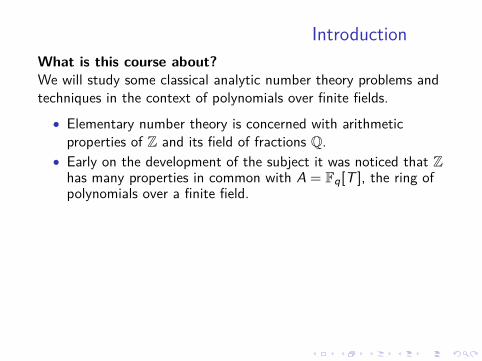
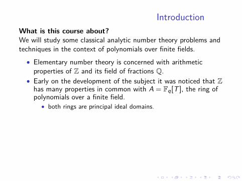
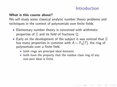
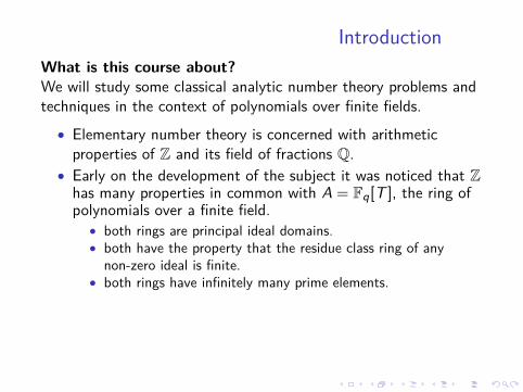
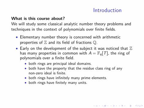
We will study some classical analytic number theory problems andtechniques in the context of polynomials over finite fields.
• Elementary number theory is concerned with arithmeticproperties of Z and its field of fractions Q.
• Early on the development of the subject it was noticed that Zhas many properties in common with A = Fq[T ], the ring ofpolynomials over a finite field.
• both rings are principal ideal domains.• both have the property that the residue class ring of any
non-zero ideal is finite.• both rings have infinitely many prime elements.• both rings have finitely many units.• ...
• Thus, one is led to suspect that many results which hold for Zhave analogues of the ring A. This is indeed the case.
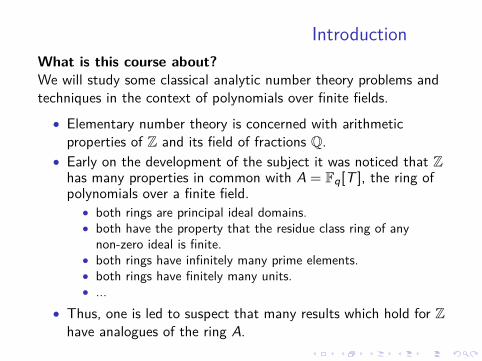
IntroductionWhat is this course about?We will study some classical analytic number theory problems andtechniques in the context of polynomials over finite fields.
• Elementary number theory is concerned with arithmeticproperties of Z and its field of fractions Q.
• Early on the development of the subject it was noticed that Zhas many properties in common with A = Fq[T ], the ring ofpolynomials over a finite field.
• both rings are principal ideal domains.• both have the property that the residue class ring of any
non-zero ideal is finite.• both rings have infinitely many prime elements.• both rings have finitely many units.• ...
• Thus, one is led to suspect that many results which hold for Zhave analogues of the ring A. This is indeed the case.
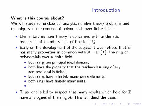
IntroductionWhat is this course about?We will study some classical analytic number theory problems andtechniques in the context of polynomials over finite fields.
• Elementary number theory is concerned with arithmeticproperties of Z and its field of fractions Q.
• Early on the development of the subject it was noticed that Zhas many properties in common with A = Fq[T ], the ring ofpolynomials over a finite field.
• both rings are principal ideal domains.• both have the property that the residue class ring of any
non-zero ideal is finite.• both rings have infinitely many prime elements.• both rings have finitely many units.• ...
• Thus, one is led to suspect that many results which hold for Zhave analogues of the ring A. This is indeed the case.
IntroductionWhat is this course about?We will study some classical analytic number theory problems andtechniques in the context of polynomials over finite fields.
• Elementary number theory is concerned with arithmeticproperties of Z and its field of fractions Q.
• Early on the development of the subject it was noticed that Zhas many properties in common with A = Fq[T ], the ring ofpolynomials over a finite field.
• both rings are principal ideal domains.
• both have the property that the residue class ring of anynon-zero ideal is finite.
• both rings have infinitely many prime elements.• both rings have finitely many units.• ...
• Thus, one is led to suspect that many results which hold for Zhave analogues of the ring A. This is indeed the case.
IntroductionWhat is this course about?We will study some classical analytic number theory problems andtechniques in the context of polynomials over finite fields.
• Elementary number theory is concerned with arithmeticproperties of Z and its field of fractions Q.
• Early on the development of the subject it was noticed that Zhas many properties in common with A = Fq[T ], the ring ofpolynomials over a finite field.
• both rings are principal ideal domains.• both have the property that the residue class ring of any
non-zero ideal is finite.
• both rings have infinitely many prime elements.• both rings have finitely many units.• ...
• Thus, one is led to suspect that many results which hold for Zhave analogues of the ring A. This is indeed the case.
IntroductionWhat is this course about?We will study some classical analytic number theory problems andtechniques in the context of polynomials over finite fields.
• Elementary number theory is concerned with arithmeticproperties of Z and its field of fractions Q.
• Early on the development of the subject it was noticed that Zhas many properties in common with A = Fq[T ], the ring ofpolynomials over a finite field.
• both rings are principal ideal domains.• both have the property that the residue class ring of any
non-zero ideal is finite.• both rings have infinitely many prime elements.
• both rings have finitely many units.• ...
• Thus, one is led to suspect that many results which hold for Zhave analogues of the ring A. This is indeed the case.
IntroductionWhat is this course about?We will study some classical analytic number theory problems andtechniques in the context of polynomials over finite fields.
• Elementary number theory is concerned with arithmeticproperties of Z and its field of fractions Q.
• Early on the development of the subject it was noticed that Zhas many properties in common with A = Fq[T ], the ring ofpolynomials over a finite field.
• both rings are principal ideal domains.• both have the property that the residue class ring of any
non-zero ideal is finite.• both rings have infinitely many prime elements.• both rings have finitely many units.
• ...• Thus, one is led to suspect that many results which hold for Z
have analogues of the ring A. This is indeed the case.

IntroductionWhat is this course about?We will study some classical analytic number theory problems andtechniques in the context of polynomials over finite fields.
• Elementary number theory is concerned with arithmeticproperties of Z and its field of fractions Q.
• Early on the development of the subject it was noticed that Zhas many properties in common with A = Fq[T ], the ring ofpolynomials over a finite field.
• both rings are principal ideal domains.• both have the property that the residue class ring of any
non-zero ideal is finite.• both rings have infinitely many prime elements.• both rings have finitely many units.• ...
• Thus, one is led to suspect that many results which hold for Zhave analogues of the ring A. This is indeed the case.
IntroductionWhat is this course about?We will study some classical analytic number theory problems andtechniques in the context of polynomials over finite fields.
• Elementary number theory is concerned with arithmeticproperties of Z and its field of fractions Q.
• Early on the development of the subject it was noticed that Zhas many properties in common with A = Fq[T ], the ring ofpolynomials over a finite field.
• both rings are principal ideal domains.• both have the property that the residue class ring of any
non-zero ideal is finite.• both rings have infinitely many prime elements.• both rings have finitely many units.• ...
• Thus, one is led to suspect that many results which hold for Zhave analogues of the ring A.
This is indeed the case.
IntroductionWhat is this course about?We will study some classical analytic number theory problems andtechniques in the context of polynomials over finite fields.
• Elementary number theory is concerned with arithmeticproperties of Z and its field of fractions Q.
• Early on the development of the subject it was noticed that Zhas many properties in common with A = Fq[T ], the ring ofpolynomials over a finite field.
• both rings are principal ideal domains.• both have the property that the residue class ring of any
non-zero ideal is finite.• both rings have infinitely many prime elements.• both rings have finitely many units.• ...
• Thus, one is led to suspect that many results which hold for Zhave analogues of the ring A. This is indeed the case.
Function Fields
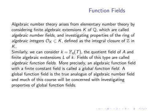
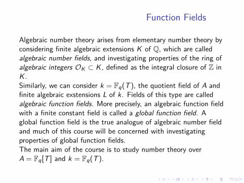
Algebraic number theory arises from elementary number theory byconsidering finite algebraic extensions K of Q, which are calledalgebraic number fields, and investigating properties of the ring ofalgebraic integers OK ⊂ K , defined as the integral closure of Z inK .
Similarly, we can consider k = Fq(T ), the quotient field of A andfinite algebraic exstensions L of k. Fields of this type are calledalgebraic function fields. More precisely, an algebraic function fieldwith a finite constant field is called a global function field. Aglobal function field is the true analogue of algebraic number fieldand much of this course will be concerned with investigatingproperties of global function fields.The main aim of the course is to study number theory overA = Fq[T ] and k = Fq(T ).
Function Fields
Algebraic number theory arises from elementary number theory byconsidering finite algebraic extensions K of Q, which are calledalgebraic number fields, and investigating properties of the ring ofalgebraic integers OK ⊂ K , defined as the integral closure of Z inK .Similarly, we can consider k = Fq(T ), the quotient field of A andfinite algebraic exstensions L of k. Fields of this type are calledalgebraic function fields. More precisely, an algebraic function fieldwith a finite constant field is called a global function field. Aglobal function field is the true analogue of algebraic number fieldand much of this course will be concerned with investigatingproperties of global function fields.
The main aim of the course is to study number theory overA = Fq[T ] and k = Fq(T ).
Function Fields
Algebraic number theory arises from elementary number theory byconsidering finite algebraic extensions K of Q, which are calledalgebraic number fields, and investigating properties of the ring ofalgebraic integers OK ⊂ K , defined as the integral closure of Z inK .Similarly, we can consider k = Fq(T ), the quotient field of A andfinite algebraic exstensions L of k. Fields of this type are calledalgebraic function fields. More precisely, an algebraic function fieldwith a finite constant field is called a global function field. Aglobal function field is the true analogue of algebraic number fieldand much of this course will be concerned with investigatingproperties of global function fields.The main aim of the course is to study number theory overA = Fq[T ] and k = Fq(T ).

The Plan for the Course
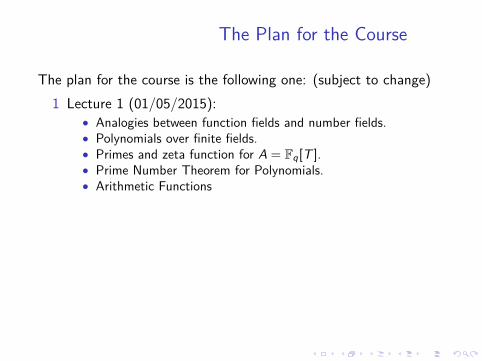
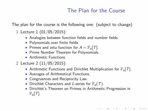
The plan for the course is the following one: (subject to change)
1 Lecture 1 (01/05/2015):• Analogies between function fields and number fields.• Polynomials over finite fields.• Primes and zeta function for A = Fq[T ].• Prime Number Theorem for Polynomials.• Arithmetic Functions
2 Lecture 2 (11/05/2015):• Arithmetic Functions and Dirichlet Multiplication for Fq[T ].• Averages of Arithmetical Functions.• Congruences and Reciprocity Law.• Dirichlet Characters and L-series for Fq(T ).• Dirichlet’s Theorem on Primes in Arithmetic Progression in
Fq[T ].
The Plan for the Course
The plan for the course is the following one: (subject to change)1 Lecture 1 (01/05/2015):
• Analogies between function fields and number fields.• Polynomials over finite fields.• Primes and zeta function for A = Fq[T ].• Prime Number Theorem for Polynomials.• Arithmetic Functions
2 Lecture 2 (11/05/2015):• Arithmetic Functions and Dirichlet Multiplication for Fq[T ].• Averages of Arithmetical Functions.• Congruences and Reciprocity Law.• Dirichlet Characters and L-series for Fq(T ).• Dirichlet’s Theorem on Primes in Arithmetic Progression in
Fq[T ].
The Plan for the Course
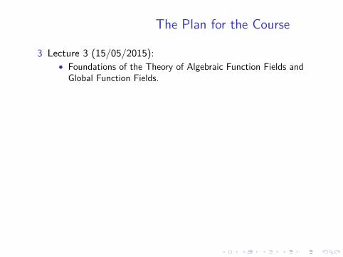
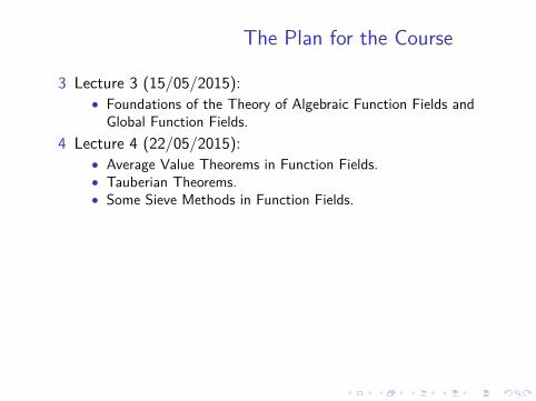
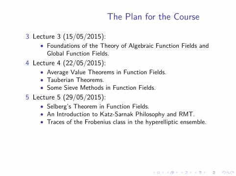
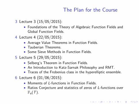
3 Lecture 3 (15/05/2015):• Foundations of the Theory of Algebraic Function Fields and
Global Function Fields.
4 Lecture 4 (22/05/2015):• Average Value Theorems in Function Fields.• Tauberian Theorems.• Some Sieve Methods in Function Fields.
5 Lecture 5 (29/05/2015):• Selberg’s Theorem in Function Fields.• An Introduction to Katz-Sarnak Philosophy and RMT.• Traces of the Frobenius class in the hyperelliptic ensemble.
6 Lecture 6 (01/06/2015):• Moments of L-functions in Function Fields.• Ratios Conjecture and statistics of zeros of L-functions over
Fq(T ).
The Plan for the Course
3 Lecture 3 (15/05/2015):• Foundations of the Theory of Algebraic Function Fields and
Global Function Fields.4 Lecture 4 (22/05/2015):
• Average Value Theorems in Function Fields.• Tauberian Theorems.• Some Sieve Methods in Function Fields.
5 Lecture 5 (29/05/2015):• Selberg’s Theorem in Function Fields.• An Introduction to Katz-Sarnak Philosophy and RMT.• Traces of the Frobenius class in the hyperelliptic ensemble.
6 Lecture 6 (01/06/2015):• Moments of L-functions in Function Fields.• Ratios Conjecture and statistics of zeros of L-functions over
Fq(T ).
The Plan for the Course
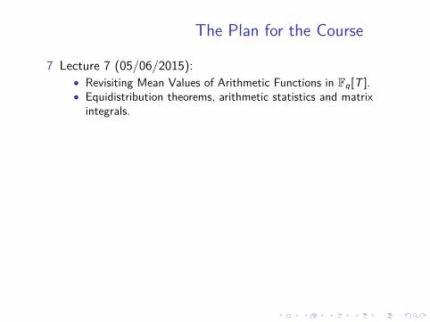
7 Lecture 7 (05/06/2015):• Revisiting Mean Values of Arithmetic Functions in Fq[T ].• Equidistribution theorems, arithmetic statistics and matrix
integrals.
8 Lecture 8 (11/06/2015):• Overview of a proof of the Function Field Riemann Hypothesis.• New directions and problems.
Assessment: At the end of the course, participants will choosefrom a list of topics/original research articles and should write upan exposition of the chosen result. This exposition should placethe result in the context of what has been discussed in the course,and should be detailed for other course participants to be able tofollow the main steps of the argument.Problem Sheets: The completion of the weekly problem sheets isoptional but strongly encouraged.
The Plan for the Course
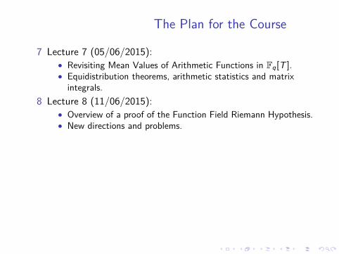
7 Lecture 7 (05/06/2015):• Revisiting Mean Values of Arithmetic Functions in Fq[T ].• Equidistribution theorems, arithmetic statistics and matrix
integrals.8 Lecture 8 (11/06/2015):
• Overview of a proof of the Function Field Riemann Hypothesis.• New directions and problems.
Assessment: At the end of the course, participants will choosefrom a list of topics/original research articles and should write upan exposition of the chosen result. This exposition should placethe result in the context of what has been discussed in the course,and should be detailed for other course participants to be able tofollow the main steps of the argument.Problem Sheets: The completion of the weekly problem sheets isoptional but strongly encouraged.
The Plan for the Course
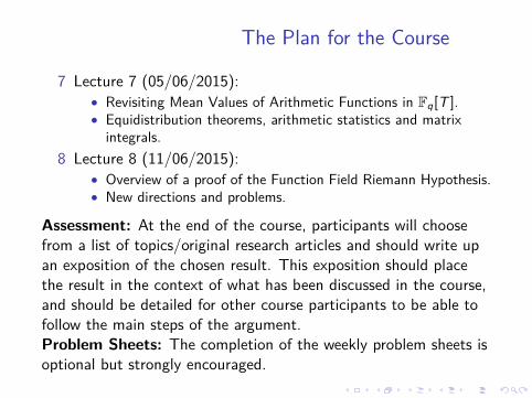
7 Lecture 7 (05/06/2015):• Revisiting Mean Values of Arithmetic Functions in Fq[T ].• Equidistribution theorems, arithmetic statistics and matrix
integrals.8 Lecture 8 (11/06/2015):
• Overview of a proof of the Function Field Riemann Hypothesis.• New directions and problems.
Assessment: At the end of the course, participants will choosefrom a list of topics/original research articles and should write upan exposition of the chosen result. This exposition should placethe result in the context of what has been discussed in the course,and should be detailed for other course participants to be able tofollow the main steps of the argument.Problem Sheets: The completion of the weekly problem sheets isoptional but strongly encouraged.
Polynomials over Finite Fields
Let Fq denote a finite field with q elements.
The model for such afield is Z/pZ, where p is a prime number. This field has pelements. In general the number of elements in a finite field is apower of a prime, q = pa. Of course, p is the characteristic of Fq.Let A = Fq[T ] be the polynomial ring over Fq. Let f ∈ A, i.e.,
f (T ) = α0T n + α1T n−1 + · · ·+ α1T + αn,
with αi ∈ Fq.
DefinitionIf α0 6= 0 we say that f has degree n, notationally deg(f ) = n. Inthis case we set sgn(f ) = α0 and call this element of F∗q the signof f .
Polynomials over Finite Fields
Let Fq denote a finite field with q elements. The model for such afield is Z/pZ, where p is a prime number. This field has pelements.
In general the number of elements in a finite field is apower of a prime, q = pa. Of course, p is the characteristic of Fq.Let A = Fq[T ] be the polynomial ring over Fq. Let f ∈ A, i.e.,
f (T ) = α0T n + α1T n−1 + · · ·+ α1T + αn,
with αi ∈ Fq.
DefinitionIf α0 6= 0 we say that f has degree n, notationally deg(f ) = n. Inthis case we set sgn(f ) = α0 and call this element of F∗q the signof f .

Polynomials over Finite Fields
Let Fq denote a finite field with q elements. The model for such afield is Z/pZ, where p is a prime number. This field has pelements. In general the number of elements in a finite field is apower of a prime, q = pa. Of course, p is the characteristic of Fq.
Let A = Fq[T ] be the polynomial ring over Fq. Let f ∈ A, i.e.,
f (T ) = α0T n + α1T n−1 + · · ·+ α1T + αn,
with αi ∈ Fq.
DefinitionIf α0 6= 0 we say that f has degree n, notationally deg(f ) = n. Inthis case we set sgn(f ) = α0 and call this element of F∗q the signof f .
Polynomials over Finite Fields
Let Fq denote a finite field with q elements. The model for such afield is Z/pZ, where p is a prime number. This field has pelements. In general the number of elements in a finite field is apower of a prime, q = pa. Of course, p is the characteristic of Fq.Let A = Fq[T ] be the polynomial ring over Fq. Let f ∈ A, i.e.,
f (T ) = α0T n + α1T n−1 + · · ·+ α1T + αn,
with αi ∈ Fq.
DefinitionIf α0 6= 0 we say that f has degree n, notationally deg(f ) = n. Inthis case we set sgn(f ) = α0 and call this element of F∗q the signof f .
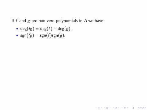
If f and g are non-zero polynomials in A we have
• deg(fg) = deg(f ) + deg(g).
• sgn(fg) = sgn(f )sgn(g).• deg(f + g) ≤ max(deg(f ), deg(g)).
(equality holds if deg(f ) 6= deg(g)).
DefinitionIf sgn(f ) = 1 we say that f is a monic polynomial.Monic polynomials play the role of positive integers.It is sometimes useful to define the sign of the zero polynomial tobe 0 and its degree −∞.
If f and g are non-zero polynomials in A we have
• deg(fg) = deg(f ) + deg(g).• sgn(fg) = sgn(f )sgn(g).
• deg(f + g) ≤ max(deg(f ), deg(g)).(equality holds if deg(f ) 6= deg(g)).
DefinitionIf sgn(f ) = 1 we say that f is a monic polynomial.Monic polynomials play the role of positive integers.It is sometimes useful to define the sign of the zero polynomial tobe 0 and its degree −∞.
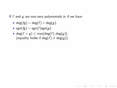
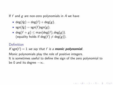
If f and g are non-zero polynomials in A we have
• deg(fg) = deg(f ) + deg(g).• sgn(fg) = sgn(f )sgn(g).• deg(f + g) ≤ max(deg(f ), deg(g)).
(equality holds if deg(f ) 6= deg(g)).
DefinitionIf sgn(f ) = 1 we say that f is a monic polynomial.Monic polynomials play the role of positive integers.It is sometimes useful to define the sign of the zero polynomial tobe 0 and its degree −∞.
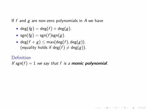
If f and g are non-zero polynomials in A we have
• deg(fg) = deg(f ) + deg(g).• sgn(fg) = sgn(f )sgn(g).• deg(f + g) ≤ max(deg(f ), deg(g)).
(equality holds if deg(f ) 6= deg(g)).
DefinitionIf sgn(f ) = 1 we say that f is a monic polynomial.
Monic polynomials play the role of positive integers.It is sometimes useful to define the sign of the zero polynomial tobe 0 and its degree −∞.
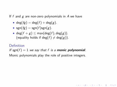
If f and g are non-zero polynomials in A we have
• deg(fg) = deg(f ) + deg(g).• sgn(fg) = sgn(f )sgn(g).• deg(f + g) ≤ max(deg(f ), deg(g)).
(equality holds if deg(f ) 6= deg(g)).
DefinitionIf sgn(f ) = 1 we say that f is a monic polynomial.Monic polynomials play the role of positive integers.
It is sometimes useful to define the sign of the zero polynomial tobe 0 and its degree −∞.
If f and g are non-zero polynomials in A we have
• deg(fg) = deg(f ) + deg(g).• sgn(fg) = sgn(f )sgn(g).• deg(f + g) ≤ max(deg(f ), deg(g)).
(equality holds if deg(f ) 6= deg(g)).
DefinitionIf sgn(f ) = 1 we say that f is a monic polynomial.Monic polynomials play the role of positive integers.It is sometimes useful to define the sign of the zero polynomial tobe 0 and its degree −∞.
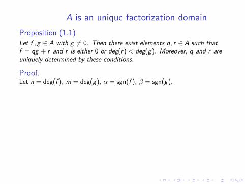
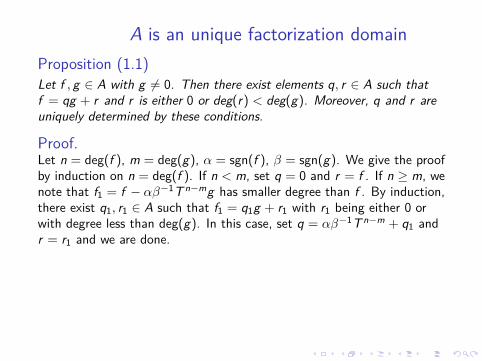
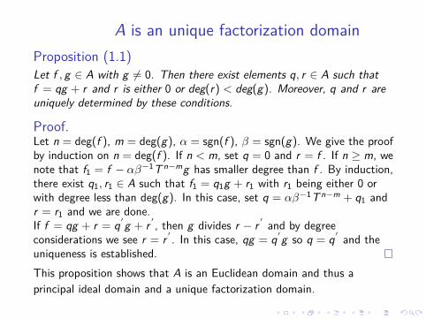
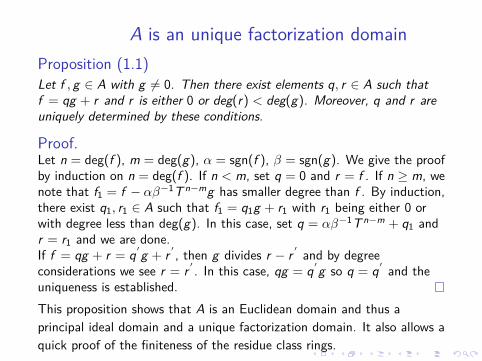
A is an unique factorization domainProposition (1.1)Let f , g ∈ A with g 6= 0. Then there exist elements q, r ∈ A such thatf = qg + r and r is either 0 or deg(r) < deg(g). Moreover, q and r areuniquely determined by these conditions.
Proof.Let n = deg(f ), m = deg(g), α = sgn(f ), β = sgn(g).
We give the proofby induction on n = deg(f ). If n < m, set q = 0 and r = f . If n ≥ m, wenote that f1 = f − αβ−1T n−mg has smaller degree than f . By induction,there exist q1, r1 ∈ A such that f1 = q1g + r1 with r1 being either 0 orwith degree less than deg(g). In this case, set q = αβ−1T n−m + q1 andr = r1 and we are done.If f = qg + r = q′ g + r ′ , then g divides r − r ′ and by degreeconsiderations we see r = r ′ . In this case, qg = q′ g so q = q′ and theuniqueness is established.This proposition shows that A is an Euclidean domain and thus aprincipal ideal domain and a unique factorization domain. It also allows aquick proof of the finiteness of the residue class rings.
A is an unique factorization domainProposition (1.1)Let f , g ∈ A with g 6= 0. Then there exist elements q, r ∈ A such thatf = qg + r and r is either 0 or deg(r) < deg(g). Moreover, q and r areuniquely determined by these conditions.
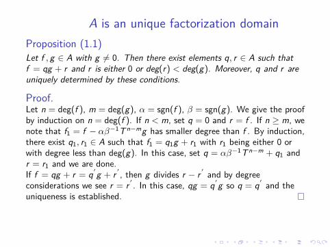
Proof.Let n = deg(f ), m = deg(g), α = sgn(f ), β = sgn(g). We give the proofby induction on n = deg(f ). If n < m, set q = 0 and r = f . If n ≥ m, wenote that f1 = f − αβ−1T n−mg has smaller degree than f . By induction,there exist q1, r1 ∈ A such that f1 = q1g + r1 with r1 being either 0 orwith degree less than deg(g). In this case, set q = αβ−1T n−m + q1 andr = r1 and we are done.
If f = qg + r = q′ g + r ′ , then g divides r − r ′ and by degreeconsiderations we see r = r ′ . In this case, qg = q′ g so q = q′ and theuniqueness is established.This proposition shows that A is an Euclidean domain and thus aprincipal ideal domain and a unique factorization domain. It also allows aquick proof of the finiteness of the residue class rings.
A is an unique factorization domainProposition (1.1)Let f , g ∈ A with g 6= 0. Then there exist elements q, r ∈ A such thatf = qg + r and r is either 0 or deg(r) < deg(g). Moreover, q and r areuniquely determined by these conditions.
Proof.Let n = deg(f ), m = deg(g), α = sgn(f ), β = sgn(g). We give the proofby induction on n = deg(f ). If n < m, set q = 0 and r = f . If n ≥ m, wenote that f1 = f − αβ−1T n−mg has smaller degree than f . By induction,there exist q1, r1 ∈ A such that f1 = q1g + r1 with r1 being either 0 orwith degree less than deg(g). In this case, set q = αβ−1T n−m + q1 andr = r1 and we are done.If f = qg + r = q′ g + r ′ , then g divides r − r ′ and by degreeconsiderations we see r = r ′ . In this case, qg = q′ g so q = q′ and theuniqueness is established.
This proposition shows that A is an Euclidean domain and thus aprincipal ideal domain and a unique factorization domain. It also allows aquick proof of the finiteness of the residue class rings.
A is an unique factorization domainProposition (1.1)Let f , g ∈ A with g 6= 0. Then there exist elements q, r ∈ A such thatf = qg + r and r is either 0 or deg(r) < deg(g). Moreover, q and r areuniquely determined by these conditions.
Proof.Let n = deg(f ), m = deg(g), α = sgn(f ), β = sgn(g). We give the proofby induction on n = deg(f ). If n < m, set q = 0 and r = f . If n ≥ m, wenote that f1 = f − αβ−1T n−mg has smaller degree than f . By induction,there exist q1, r1 ∈ A such that f1 = q1g + r1 with r1 being either 0 orwith degree less than deg(g). In this case, set q = αβ−1T n−m + q1 andr = r1 and we are done.If f = qg + r = q′ g + r ′ , then g divides r − r ′ and by degreeconsiderations we see r = r ′ . In this case, qg = q′ g so q = q′ and theuniqueness is established.This proposition shows that A is an Euclidean domain and thus aprincipal ideal domain and a unique factorization domain.
It also allows aquick proof of the finiteness of the residue class rings.
A is an unique factorization domainProposition (1.1)Let f , g ∈ A with g 6= 0. Then there exist elements q, r ∈ A such thatf = qg + r and r is either 0 or deg(r) < deg(g). Moreover, q and r areuniquely determined by these conditions.
Proof.Let n = deg(f ), m = deg(g), α = sgn(f ), β = sgn(g). We give the proofby induction on n = deg(f ). If n < m, set q = 0 and r = f . If n ≥ m, wenote that f1 = f − αβ−1T n−mg has smaller degree than f . By induction,there exist q1, r1 ∈ A such that f1 = q1g + r1 with r1 being either 0 orwith degree less than deg(g). In this case, set q = αβ−1T n−m + q1 andr = r1 and we are done.If f = qg + r = q′ g + r ′ , then g divides r − r ′ and by degreeconsiderations we see r = r ′ . In this case, qg = q′ g so q = q′ and theuniqueness is established.This proposition shows that A is an Euclidean domain and thus aprincipal ideal domain and a unique factorization domain. It also allows aquick proof of the finiteness of the residue class rings.
Finiteness of the Residue Class Rings
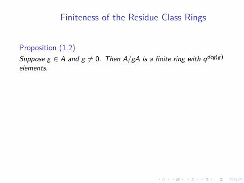
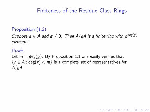
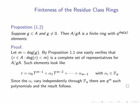
Proposition (1.2)Suppose g ∈ A and g 6= 0. Then A/gA is a finite ring with qdeg(g)
elements.
Proof.Let m = deg(g). By Proposition 1.1 one easily verifies that{r ∈ A : deg(r) < m} is a complete set of representatives forA/gA. Such elements look like
r = α0T m−1 + α1T m−2 + · · ·+ αm−1 with αi ∈ Fq.
Since the αi vary independently through Fq there are qm suchpolynomials and the result follows.
Finiteness of the Residue Class Rings
Proposition (1.2)Suppose g ∈ A and g 6= 0. Then A/gA is a finite ring with qdeg(g)
elements.
Proof.Let m = deg(g). By Proposition 1.1 one easily verifies that{r ∈ A : deg(r) < m} is a complete set of representatives forA/gA.
Such elements look like
r = α0T m−1 + α1T m−2 + · · ·+ αm−1 with αi ∈ Fq.
Since the αi vary independently through Fq there are qm suchpolynomials and the result follows.
Finiteness of the Residue Class Rings
Proposition (1.2)Suppose g ∈ A and g 6= 0. Then A/gA is a finite ring with qdeg(g)
elements.
Proof.Let m = deg(g). By Proposition 1.1 one easily verifies that{r ∈ A : deg(r) < m} is a complete set of representatives forA/gA. Such elements look like
r = α0T m−1 + α1T m−2 + · · ·+ αm−1 with αi ∈ Fq.
Since the αi vary independently through Fq there are qm suchpolynomials and the result follows.
Norm of a Polynomial
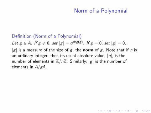
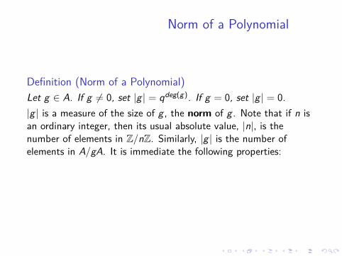
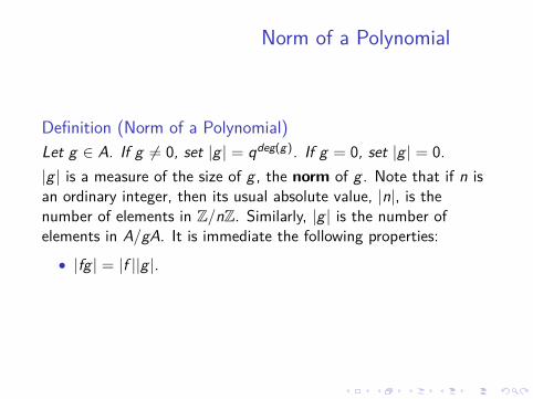
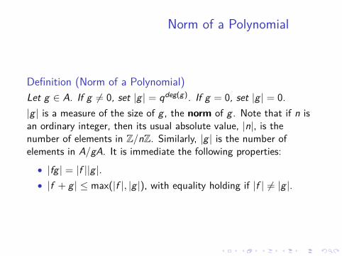
Definition (Norm of a Polynomial)Let g ∈ A. If g 6= 0, set |g | = qdeg(g). If g = 0, set |g | = 0.
|g | is a measure of the size of g , the norm of g . Note that if n isan ordinary integer, then its usual absolute value, |n|, is thenumber of elements in Z/nZ. Similarly, |g | is the number ofelements in A/gA. It is immediate the following properties:
• |fg | = |f ||g |.• |f + g | ≤ max(|f |, |g |), with equality holding if |f | 6= |g |.
Norm of a Polynomial
Definition (Norm of a Polynomial)Let g ∈ A. If g 6= 0, set |g | = qdeg(g). If g = 0, set |g | = 0.|g | is a measure of the size of g , the norm of g .
Note that if n isan ordinary integer, then its usual absolute value, |n|, is thenumber of elements in Z/nZ. Similarly, |g | is the number ofelements in A/gA. It is immediate the following properties:
• |fg | = |f ||g |.• |f + g | ≤ max(|f |, |g |), with equality holding if |f | 6= |g |.
Norm of a Polynomial
Definition (Norm of a Polynomial)Let g ∈ A. If g 6= 0, set |g | = qdeg(g). If g = 0, set |g | = 0.|g | is a measure of the size of g , the norm of g . Note that if n isan ordinary integer, then its usual absolute value, |n|, is thenumber of elements in Z/nZ.
Similarly, |g | is the number ofelements in A/gA. It is immediate the following properties:
• |fg | = |f ||g |.• |f + g | ≤ max(|f |, |g |), with equality holding if |f | 6= |g |.
Norm of a Polynomial
Definition (Norm of a Polynomial)Let g ∈ A. If g 6= 0, set |g | = qdeg(g). If g = 0, set |g | = 0.|g | is a measure of the size of g , the norm of g . Note that if n isan ordinary integer, then its usual absolute value, |n|, is thenumber of elements in Z/nZ. Similarly, |g | is the number ofelements in A/gA.
It is immediate the following properties:
• |fg | = |f ||g |.• |f + g | ≤ max(|f |, |g |), with equality holding if |f | 6= |g |.
Norm of a Polynomial
Definition (Norm of a Polynomial)Let g ∈ A. If g 6= 0, set |g | = qdeg(g). If g = 0, set |g | = 0.|g | is a measure of the size of g , the norm of g . Note that if n isan ordinary integer, then its usual absolute value, |n|, is thenumber of elements in Z/nZ. Similarly, |g | is the number ofelements in A/gA. It is immediate the following properties:
• |fg | = |f ||g |.
• |f + g | ≤ max(|f |, |g |), with equality holding if |f | 6= |g |.
Norm of a Polynomial
Definition (Norm of a Polynomial)Let g ∈ A. If g 6= 0, set |g | = qdeg(g). If g = 0, set |g | = 0.|g | is a measure of the size of g , the norm of g . Note that if n isan ordinary integer, then its usual absolute value, |n|, is thenumber of elements in Z/nZ. Similarly, |g | is the number ofelements in A/gA. It is immediate the following properties:
• |fg | = |f ||g |.• |f + g | ≤ max(|f |, |g |), with equality holding if |f | 6= |g |.
Group of Units
It is a simple matter to determine the group of units in A, A∗. If gis a unit, then there is an f such that fg = 1. Thus,0 = deg(1) = deg(f ) + deg(g) and so deg(f ) = deg(g) = 0.
Theonly units are non-zero constants and each such constant is a unit.
Proposition (1.3)The group of units in A is F∗q. In particular, it is a finite cyclicgroup with q − 1 elements.
Proof.The only thing left to prove is the cyclicity of F∗q. This followsfrom the very general fact that a finite subgroup of themultiplicative group of a field is cyclic.In what follows we will see that the number q − 1 often occurswhere the number 2 occurs in ordinary number theory. This stemsfrom the fact that the order of Z∗ is 2.
Group of Units
It is a simple matter to determine the group of units in A, A∗. If gis a unit, then there is an f such that fg = 1. Thus,0 = deg(1) = deg(f ) + deg(g) and so deg(f ) = deg(g) = 0. Theonly units are non-zero constants and each such constant is a unit.
Proposition (1.3)The group of units in A is F∗q. In particular, it is a finite cyclicgroup with q − 1 elements.
Proof.The only thing left to prove is the cyclicity of F∗q. This followsfrom the very general fact that a finite subgroup of themultiplicative group of a field is cyclic.
In what follows we will see that the number q − 1 often occurswhere the number 2 occurs in ordinary number theory. This stemsfrom the fact that the order of Z∗ is 2.
Group of Units
It is a simple matter to determine the group of units in A, A∗. If gis a unit, then there is an f such that fg = 1. Thus,0 = deg(1) = deg(f ) + deg(g) and so deg(f ) = deg(g) = 0. Theonly units are non-zero constants and each such constant is a unit.
Proposition (1.3)The group of units in A is F∗q. In particular, it is a finite cyclicgroup with q − 1 elements.
Proof.The only thing left to prove is the cyclicity of F∗q. This followsfrom the very general fact that a finite subgroup of themultiplicative group of a field is cyclic.In what follows we will see that the number q − 1 often occurswhere the number 2 occurs in ordinary number theory. This stemsfrom the fact that the order of Z∗ is 2.
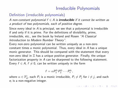
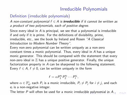
Irreducible PolynomialsDefinition (irreducible polynomials)A non-constant polynomial f ∈ A is irreducible if it cannot be written asa product of two polynomials, each of positive degree.
Since every ideal in A is principal, we see that a polynomial is irreducibleif and only if it is prime. For the definitions of divisibility, prime,irreducible, etc., see the book by Ireland and Rosen “A ClassicalIntroduction to Modern Number Theory”.Every non-zero polynomial can be written uniquely as a non-zeroconstant times a monic polynomial. Thus, every ideal in A has a uniquemonic generator. This should be compared with the statement that everynon-zero ideal in Z has a unique positive generator. Finally, the uniquefactorization property in A can be sharpened to the following statement.Every f ∈ A, f 6= 0, can be written uniquely in the form
f = αPe11 Pe2
2 · · ·Pett ,
where α ∈ F∗q, each Pi is a monic irreducible, Pi 6= Pj for i 6= j , and eachei is a non-negative integer.The letter P will often be used for a monic irreducible polynomial in A.
Irreducible PolynomialsDefinition (irreducible polynomials)A non-constant polynomial f ∈ A is irreducible if it cannot be written asa product of two polynomials, each of positive degree.Since every ideal in A is principal, we see that a polynomial is irreducibleif and only if it is prime.
For the definitions of divisibility, prime,irreducible, etc., see the book by Ireland and Rosen “A ClassicalIntroduction to Modern Number Theory”.Every non-zero polynomial can be written uniquely as a non-zeroconstant times a monic polynomial. Thus, every ideal in A has a uniquemonic generator. This should be compared with the statement that everynon-zero ideal in Z has a unique positive generator. Finally, the uniquefactorization property in A can be sharpened to the following statement.Every f ∈ A, f 6= 0, can be written uniquely in the form
f = αPe11 Pe2
2 · · ·Pett ,
where α ∈ F∗q, each Pi is a monic irreducible, Pi 6= Pj for i 6= j , and eachei is a non-negative integer.The letter P will often be used for a monic irreducible polynomial in A.
Irreducible PolynomialsDefinition (irreducible polynomials)A non-constant polynomial f ∈ A is irreducible if it cannot be written asa product of two polynomials, each of positive degree.Since every ideal in A is principal, we see that a polynomial is irreducibleif and only if it is prime. For the definitions of divisibility, prime,irreducible, etc., see the book by Ireland and Rosen “A ClassicalIntroduction to Modern Number Theory”.
Every non-zero polynomial can be written uniquely as a non-zeroconstant times a monic polynomial. Thus, every ideal in A has a uniquemonic generator. This should be compared with the statement that everynon-zero ideal in Z has a unique positive generator. Finally, the uniquefactorization property in A can be sharpened to the following statement.Every f ∈ A, f 6= 0, can be written uniquely in the form
f = αPe11 Pe2
2 · · ·Pett ,
where α ∈ F∗q, each Pi is a monic irreducible, Pi 6= Pj for i 6= j , and eachei is a non-negative integer.The letter P will often be used for a monic irreducible polynomial in A.
Irreducible PolynomialsDefinition (irreducible polynomials)A non-constant polynomial f ∈ A is irreducible if it cannot be written asa product of two polynomials, each of positive degree.Since every ideal in A is principal, we see that a polynomial is irreducibleif and only if it is prime. For the definitions of divisibility, prime,irreducible, etc., see the book by Ireland and Rosen “A ClassicalIntroduction to Modern Number Theory”.Every non-zero polynomial can be written uniquely as a non-zeroconstant times a monic polynomial.
Thus, every ideal in A has a uniquemonic generator. This should be compared with the statement that everynon-zero ideal in Z has a unique positive generator. Finally, the uniquefactorization property in A can be sharpened to the following statement.Every f ∈ A, f 6= 0, can be written uniquely in the form
f = αPe11 Pe2
2 · · ·Pett ,
where α ∈ F∗q, each Pi is a monic irreducible, Pi 6= Pj for i 6= j , and eachei is a non-negative integer.The letter P will often be used for a monic irreducible polynomial in A.
Irreducible PolynomialsDefinition (irreducible polynomials)A non-constant polynomial f ∈ A is irreducible if it cannot be written asa product of two polynomials, each of positive degree.Since every ideal in A is principal, we see that a polynomial is irreducibleif and only if it is prime. For the definitions of divisibility, prime,irreducible, etc., see the book by Ireland and Rosen “A ClassicalIntroduction to Modern Number Theory”.Every non-zero polynomial can be written uniquely as a non-zeroconstant times a monic polynomial. Thus, every ideal in A has a uniquemonic generator. This should be compared with the statement that everynon-zero ideal in Z has a unique positive generator.
Finally, the uniquefactorization property in A can be sharpened to the following statement.Every f ∈ A, f 6= 0, can be written uniquely in the form
f = αPe11 Pe2
2 · · ·Pett ,
where α ∈ F∗q, each Pi is a monic irreducible, Pi 6= Pj for i 6= j , and eachei is a non-negative integer.The letter P will often be used for a monic irreducible polynomial in A.
Irreducible PolynomialsDefinition (irreducible polynomials)A non-constant polynomial f ∈ A is irreducible if it cannot be written asa product of two polynomials, each of positive degree.Since every ideal in A is principal, we see that a polynomial is irreducibleif and only if it is prime. For the definitions of divisibility, prime,irreducible, etc., see the book by Ireland and Rosen “A ClassicalIntroduction to Modern Number Theory”.Every non-zero polynomial can be written uniquely as a non-zeroconstant times a monic polynomial. Thus, every ideal in A has a uniquemonic generator. This should be compared with the statement that everynon-zero ideal in Z has a unique positive generator. Finally, the uniquefactorization property in A can be sharpened to the following statement.
Every f ∈ A, f 6= 0, can be written uniquely in the form
f = αPe11 Pe2
2 · · ·Pett ,
where α ∈ F∗q, each Pi is a monic irreducible, Pi 6= Pj for i 6= j , and eachei is a non-negative integer.The letter P will often be used for a monic irreducible polynomial in A.
Irreducible PolynomialsDefinition (irreducible polynomials)A non-constant polynomial f ∈ A is irreducible if it cannot be written asa product of two polynomials, each of positive degree.Since every ideal in A is principal, we see that a polynomial is irreducibleif and only if it is prime. For the definitions of divisibility, prime,irreducible, etc., see the book by Ireland and Rosen “A ClassicalIntroduction to Modern Number Theory”.Every non-zero polynomial can be written uniquely as a non-zeroconstant times a monic polynomial. Thus, every ideal in A has a uniquemonic generator. This should be compared with the statement that everynon-zero ideal in Z has a unique positive generator. Finally, the uniquefactorization property in A can be sharpened to the following statement.Every f ∈ A, f 6= 0, can be written uniquely in the form
f = αPe11 Pe2
2 · · ·Pett ,
where α ∈ F∗q, each Pi is a monic irreducible, Pi 6= Pj for i 6= j , and eachei is a non-negative integer.
The letter P will often be used for a monic irreducible polynomial in A.
Irreducible PolynomialsDefinition (irreducible polynomials)A non-constant polynomial f ∈ A is irreducible if it cannot be written asa product of two polynomials, each of positive degree.Since every ideal in A is principal, we see that a polynomial is irreducibleif and only if it is prime. For the definitions of divisibility, prime,irreducible, etc., see the book by Ireland and Rosen “A ClassicalIntroduction to Modern Number Theory”.Every non-zero polynomial can be written uniquely as a non-zeroconstant times a monic polynomial. Thus, every ideal in A has a uniquemonic generator. This should be compared with the statement that everynon-zero ideal in Z has a unique positive generator. Finally, the uniquefactorization property in A can be sharpened to the following statement.Every f ∈ A, f 6= 0, can be written uniquely in the form
f = αPe11 Pe2
2 · · ·Pett ,
where α ∈ F∗q, each Pi is a monic irreducible, Pi 6= Pj for i 6= j , and eachei is a non-negative integer.The letter P will often be used for a monic irreducible polynomial in A.
The rings A/fA
The next order of business is to investigate the structure of the ringsA/fA and the unit groups (A/fA)∗.
Proposition (Chinese Remainder Theorem)Let m1,m2, . . . ,mt be elements of A which are pairwise relatively prime.Let m = m1m2 . . .mt and φi be the natural homomorphism from A/mAto A/mi A. Then, the map φ : A/mA→ A/m1A⊕A/m2A⊕ · · · ⊕A/mtAgiven by
φ(a) = (φ1(a), φ2(a), . . . , φt(a))
is a ring isomorphism.
Proof.This is a standard result which holds in any principal ideal domain(properly formulated it holds in much greater generality).
The rings A/fA
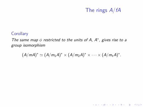
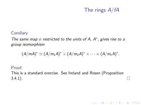
CorollaryThe same map φ restricted to the units of A, A∗, gives rise to agroup isomorphism
(A/mA)∗ ' (A/m1A)∗ × (A/m2A)∗ × · · · × (A/mtA)∗.
Proof.This is a standard exercise. See Ireland and Rosen (Proposition3.4.1).
The rings A/fA
CorollaryThe same map φ restricted to the units of A, A∗, gives rise to agroup isomorphism
(A/mA)∗ ' (A/m1A)∗ × (A/m2A)∗ × · · · × (A/mtA)∗.
Proof.This is a standard exercise. See Ireland and Rosen (Proposition3.4.1).
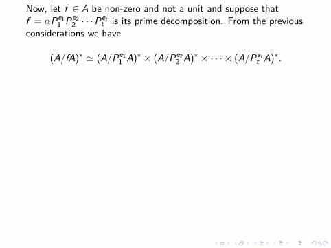
Now, let f ∈ A be non-zero and not a unit and suppose thatf = αPe1
1 Pe22 · · ·P
ett is its prime decomposition. From the previous
considerations we have
(A/fA)∗ ' (A/Pe11 A)∗ × (A/Pe2
2 A)∗ × · · · × (A/Pett A)∗.
This isomorphism reduces our task to that of determining thestructure of the groups (A/PeA)∗ where P is an irreduciblepolynomial and e is a positive integer. When e = 1 the situation isvery similar to that in Z.Proposition (1.5)Let P ∈ A be an irreducible polynomial. Then, (A/PA)∗ is a cyclicgroup with |P| − 1 elements.
Proof.Since A is a principal ideal domain, PA is a maximal ideal and soA/PA is a field. A finite subgroup of the multiplicative group of afield is cyclic. Thus (A/PA)∗ is cyclic. That the order of this groupis |P| − 1 is immediate.
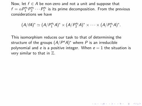
Now, let f ∈ A be non-zero and not a unit and suppose thatf = αPe1
1 Pe22 · · ·P
ett is its prime decomposition. From the previous
considerations we have
(A/fA)∗ ' (A/Pe11 A)∗ × (A/Pe2
2 A)∗ × · · · × (A/Pett A)∗.
This isomorphism reduces our task to that of determining thestructure of the groups (A/PeA)∗ where P is an irreduciblepolynomial and e is a positive integer. When e = 1 the situation isvery similar to that in Z.
Proposition (1.5)Let P ∈ A be an irreducible polynomial. Then, (A/PA)∗ is a cyclicgroup with |P| − 1 elements.
Proof.Since A is a principal ideal domain, PA is a maximal ideal and soA/PA is a field. A finite subgroup of the multiplicative group of afield is cyclic. Thus (A/PA)∗ is cyclic. That the order of this groupis |P| − 1 is immediate.
Now, let f ∈ A be non-zero and not a unit and suppose thatf = αPe1
1 Pe22 · · ·P
ett is its prime decomposition. From the previous
considerations we have
(A/fA)∗ ' (A/Pe11 A)∗ × (A/Pe2
2 A)∗ × · · · × (A/Pett A)∗.
This isomorphism reduces our task to that of determining thestructure of the groups (A/PeA)∗ where P is an irreduciblepolynomial and e is a positive integer. When e = 1 the situation isvery similar to that in Z.Proposition (1.5)Let P ∈ A be an irreducible polynomial. Then, (A/PA)∗ is a cyclicgroup with |P| − 1 elements.
Proof.Since A is a principal ideal domain, PA is a maximal ideal and soA/PA is a field. A finite subgroup of the multiplicative group of afield is cyclic. Thus (A/PA)∗ is cyclic. That the order of this groupis |P| − 1 is immediate.
Now, let f ∈ A be non-zero and not a unit and suppose thatf = αPe1
1 Pe22 · · ·P
ett is its prime decomposition. From the previous
considerations we have
(A/fA)∗ ' (A/Pe11 A)∗ × (A/Pe2
2 A)∗ × · · · × (A/Pett A)∗.
This isomorphism reduces our task to that of determining thestructure of the groups (A/PeA)∗ where P is an irreduciblepolynomial and e is a positive integer. When e = 1 the situation isvery similar to that in Z.Proposition (1.5)Let P ∈ A be an irreducible polynomial. Then, (A/PA)∗ is a cyclicgroup with |P| − 1 elements.
Proof.Since A is a principal ideal domain, PA is a maximal ideal and soA/PA is a field. A finite subgroup of the multiplicative group of afield is cyclic. Thus (A/PA)∗ is cyclic.
That the order of this groupis |P| − 1 is immediate.
Now, let f ∈ A be non-zero and not a unit and suppose thatf = αPe1
1 Pe22 · · ·P
ett is its prime decomposition. From the previous
considerations we have
(A/fA)∗ ' (A/Pe11 A)∗ × (A/Pe2
2 A)∗ × · · · × (A/Pett A)∗.
This isomorphism reduces our task to that of determining thestructure of the groups (A/PeA)∗ where P is an irreduciblepolynomial and e is a positive integer. When e = 1 the situation isvery similar to that in Z.Proposition (1.5)Let P ∈ A be an irreducible polynomial. Then, (A/PA)∗ is a cyclicgroup with |P| − 1 elements.
Proof.Since A is a principal ideal domain, PA is a maximal ideal and soA/PA is a field. A finite subgroup of the multiplicative group of afield is cyclic. Thus (A/PA)∗ is cyclic. That the order of this groupis |P| − 1 is immediate.
Contrast between A = Fq[T ] and Z
We now consider the situation when e > 1.
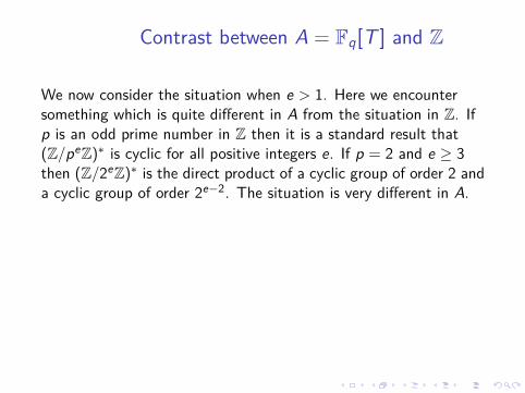
Here we encountersomething which is quite different in A from the situation in Z. Ifp is an odd prime number in Z then it is a standard result that(Z/peZ)∗ is cyclic for all positive integers e. If p = 2 and e ≥ 3then (Z/2eZ)∗ is the direct product of a cyclic group of order 2 anda cyclic group of order 2e−2. The situation is very different in A.
Proposition (1.6)Let P ∈ A be an irreducible polynomial and e a positive integer.The order of (A/PeA)∗ is |P|e−1(|P| − 1). Let (A/PeA)(1) be thekernel of the natural map from (A/PeA)∗ to (A/PA)∗. It is ap-group of order |P|e−1. As e tends to infinity, the minimalnumber of generators of (A/PeA)(1) tends to infinity.
Contrast between A = Fq[T ] and Z
We now consider the situation when e > 1. Here we encountersomething which is quite different in A from the situation in Z.
Ifp is an odd prime number in Z then it is a standard result that(Z/peZ)∗ is cyclic for all positive integers e. If p = 2 and e ≥ 3then (Z/2eZ)∗ is the direct product of a cyclic group of order 2 anda cyclic group of order 2e−2. The situation is very different in A.
Proposition (1.6)Let P ∈ A be an irreducible polynomial and e a positive integer.The order of (A/PeA)∗ is |P|e−1(|P| − 1). Let (A/PeA)(1) be thekernel of the natural map from (A/PeA)∗ to (A/PA)∗. It is ap-group of order |P|e−1. As e tends to infinity, the minimalnumber of generators of (A/PeA)(1) tends to infinity.
Contrast between A = Fq[T ] and Z
We now consider the situation when e > 1. Here we encountersomething which is quite different in A from the situation in Z. Ifp is an odd prime number in Z then it is a standard result that(Z/peZ)∗ is cyclic for all positive integers e. If p = 2 and e ≥ 3then (Z/2eZ)∗ is the direct product of a cyclic group of order 2 anda cyclic group of order 2e−2. The situation is very different in A.
Proposition (1.6)Let P ∈ A be an irreducible polynomial and e a positive integer.The order of (A/PeA)∗ is |P|e−1(|P| − 1). Let (A/PeA)(1) be thekernel of the natural map from (A/PeA)∗ to (A/PA)∗. It is ap-group of order |P|e−1. As e tends to infinity, the minimalnumber of generators of (A/PeA)(1) tends to infinity.
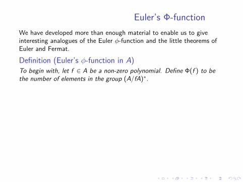
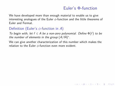
Euler’s Φ-functionWe have developed more than enough material to enable us to giveinteresting analogues of the Euler φ-function and the little theorems ofEuler and Fermat.
Definition (Euler’s φ-function in A)To begin with, let f ∈ A be a non-zero polynomial. Define Φ(f ) to bethe number of elements in the group (A/fA)∗.We can give another characterization of this number which makes therelation to the Euler φ-function even more evident. We have seen that{r ∈ A : deg(r) < deg(f )} is a set or representatives for A/fA. Such an rrepresents a unit in A/fA if and only if it is relatively prime to f . ThusΦ(f ) is the number of non-zero polynomials of degree less than deg(f )and relatively prime to f , i.e.
Φ(f ) =∑
k monicdeg(k)<deg(f )
gcd(f ,k)=1
1.
Euler’s Φ-functionWe have developed more than enough material to enable us to giveinteresting analogues of the Euler φ-function and the little theorems ofEuler and Fermat.
Definition (Euler’s φ-function in A)To begin with, let f ∈ A be a non-zero polynomial. Define Φ(f ) to bethe number of elements in the group (A/fA)∗.
We can give another characterization of this number which makes therelation to the Euler φ-function even more evident. We have seen that{r ∈ A : deg(r) < deg(f )} is a set or representatives for A/fA. Such an rrepresents a unit in A/fA if and only if it is relatively prime to f . ThusΦ(f ) is the number of non-zero polynomials of degree less than deg(f )and relatively prime to f , i.e.
Φ(f ) =∑
k monicdeg(k)<deg(f )
gcd(f ,k)=1
1.
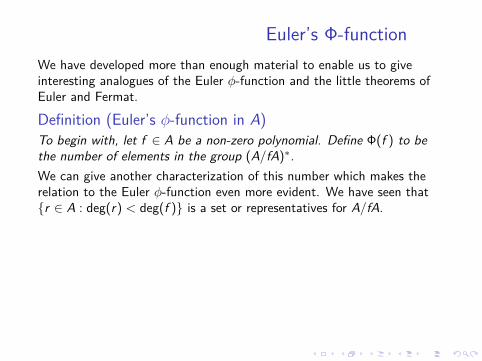
Euler’s Φ-functionWe have developed more than enough material to enable us to giveinteresting analogues of the Euler φ-function and the little theorems ofEuler and Fermat.
Definition (Euler’s φ-function in A)To begin with, let f ∈ A be a non-zero polynomial. Define Φ(f ) to bethe number of elements in the group (A/fA)∗.We can give another characterization of this number which makes therelation to the Euler φ-function even more evident.
We have seen that{r ∈ A : deg(r) < deg(f )} is a set or representatives for A/fA. Such an rrepresents a unit in A/fA if and only if it is relatively prime to f . ThusΦ(f ) is the number of non-zero polynomials of degree less than deg(f )and relatively prime to f , i.e.
Φ(f ) =∑
k monicdeg(k)<deg(f )
gcd(f ,k)=1
1.
Euler’s Φ-functionWe have developed more than enough material to enable us to giveinteresting analogues of the Euler φ-function and the little theorems ofEuler and Fermat.
Definition (Euler’s φ-function in A)To begin with, let f ∈ A be a non-zero polynomial. Define Φ(f ) to bethe number of elements in the group (A/fA)∗.We can give another characterization of this number which makes therelation to the Euler φ-function even more evident. We have seen that{r ∈ A : deg(r) < deg(f )} is a set or representatives for A/fA.
Such an rrepresents a unit in A/fA if and only if it is relatively prime to f . ThusΦ(f ) is the number of non-zero polynomials of degree less than deg(f )and relatively prime to f , i.e.
Φ(f ) =∑
k monicdeg(k)<deg(f )
gcd(f ,k)=1
1.

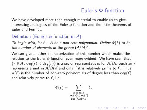
Euler’s Φ-functionWe have developed more than enough material to enable us to giveinteresting analogues of the Euler φ-function and the little theorems ofEuler and Fermat.
Definition (Euler’s φ-function in A)To begin with, let f ∈ A be a non-zero polynomial. Define Φ(f ) to bethe number of elements in the group (A/fA)∗.We can give another characterization of this number which makes therelation to the Euler φ-function even more evident. We have seen that{r ∈ A : deg(r) < deg(f )} is a set or representatives for A/fA. Such an rrepresents a unit in A/fA if and only if it is relatively prime to f .
ThusΦ(f ) is the number of non-zero polynomials of degree less than deg(f )and relatively prime to f , i.e.
Φ(f ) =∑
k monicdeg(k)<deg(f )
gcd(f ,k)=1
1.
Euler’s Φ-functionWe have developed more than enough material to enable us to giveinteresting analogues of the Euler φ-function and the little theorems ofEuler and Fermat.
Definition (Euler’s φ-function in A)To begin with, let f ∈ A be a non-zero polynomial. Define Φ(f ) to bethe number of elements in the group (A/fA)∗.We can give another characterization of this number which makes therelation to the Euler φ-function even more evident. We have seen that{r ∈ A : deg(r) < deg(f )} is a set or representatives for A/fA. Such an rrepresents a unit in A/fA if and only if it is relatively prime to f . ThusΦ(f ) is the number of non-zero polynomials of degree less than deg(f )and relatively prime to f , i.e.
Φ(f ) =∑
k monicdeg(k)<deg(f )
gcd(f ,k)=1
1.
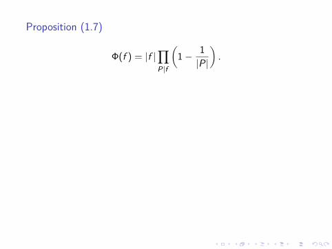
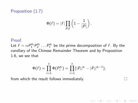
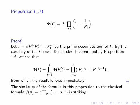
Proposition (1.7)
Φ(f ) = |f |∏P|f
(1− 1|P|
).
Proof.Let f = αPe1
1 Pe22 . . .Pet
t be the prime decomposition of f . By thecorollary of the Chinese Remainder Theorem and by Proposition1.6, we see that
Φ(f ) =t∏
i=1Φ(Pei
i ) =t∏
i=1(|Pi |ei − |Pi |ei−1),
from which the result follows immediately.The similarity of the formula in this proposition to the classicalformula φ(n) = n
∏p|n(1− p−1) is striking.
Proposition (1.7)
Φ(f ) = |f |∏P|f
(1− 1|P|
).
Proof.Let f = αPe1
1 Pe22 . . .Pet
t be the prime decomposition of f . By thecorollary of the Chinese Remainder Theorem and by Proposition1.6, we see that
Φ(f ) =t∏
i=1Φ(Pei
i ) =t∏
i=1(|Pi |ei − |Pi |ei−1),
from which the result follows immediately.
The similarity of the formula in this proposition to the classicalformula φ(n) = n
∏p|n(1− p−1) is striking.
Proposition (1.7)
Φ(f ) = |f |∏P|f
(1− 1|P|
).
Proof.Let f = αPe1
1 Pe22 . . .Pet
t be the prime decomposition of f . By thecorollary of the Chinese Remainder Theorem and by Proposition1.6, we see that
Φ(f ) =t∏
i=1Φ(Pei
i ) =t∏
i=1(|Pi |ei − |Pi |ei−1),
from which the result follows immediately.The similarity of the formula in this proposition to the classicalformula φ(n) = n
∏p|n(1− p−1) is striking.
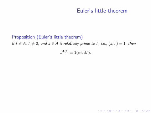
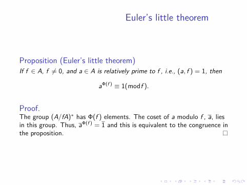
Euler’s little theorem
Proposition (Euler’s little theorem)If f ∈ A, f 6= 0, and a ∈ A is relatively prime to f , i.e., (a, f ) = 1, then
aΦ(f ) ≡ 1(modf ).
Proof.The group (A/fA)∗ has Φ(f ) elements. The coset of a modulo f , a, liesin this group. Thus, aΦ(f ) = 1 and this is equivalent to the congruence inthe proposition.
Fermat’s little theorem
Corollary (Fermat’s little theorem)Let P ∈ A be irreducible and a ∈ A be a polynomial not divisibleby P. Then,
a|P|−1 ≡ 1(modP).
Proof.Since P is irreducible, it is relatively prime to a if and only if itdoes not divide a. The corollary follows from the proposition andthe fact that for an irreducible P, Φ(P) = |P| − 1 (Proposition1.5).The theorems above play the same very important role in thiscontext as they do in elementary number theory. By way ofillustration we proceed to the analogue of Wilson’s theorem. Recallthat this states that (p − 1)! ≡ −1(modp) where p is a primenumber.

Fermat’s little theorem
Corollary (Fermat’s little theorem)Let P ∈ A be irreducible and a ∈ A be a polynomial not divisibleby P. Then,
a|P|−1 ≡ 1(modP).
Proof.Since P is irreducible, it is relatively prime to a if and only if itdoes not divide a. The corollary follows from the proposition andthe fact that for an irreducible P, Φ(P) = |P| − 1 (Proposition1.5).
The theorems above play the same very important role in thiscontext as they do in elementary number theory. By way ofillustration we proceed to the analogue of Wilson’s theorem. Recallthat this states that (p − 1)! ≡ −1(modp) where p is a primenumber.
Fermat’s little theorem
Corollary (Fermat’s little theorem)Let P ∈ A be irreducible and a ∈ A be a polynomial not divisibleby P. Then,
a|P|−1 ≡ 1(modP).
Proof.Since P is irreducible, it is relatively prime to a if and only if itdoes not divide a. The corollary follows from the proposition andthe fact that for an irreducible P, Φ(P) = |P| − 1 (Proposition1.5).The theorems above play the same very important role in thiscontext as they do in elementary number theory.
By way ofillustration we proceed to the analogue of Wilson’s theorem. Recallthat this states that (p − 1)! ≡ −1(modp) where p is a primenumber.
Fermat’s little theorem
Corollary (Fermat’s little theorem)Let P ∈ A be irreducible and a ∈ A be a polynomial not divisibleby P. Then,
a|P|−1 ≡ 1(modP).
Proof.Since P is irreducible, it is relatively prime to a if and only if itdoes not divide a. The corollary follows from the proposition andthe fact that for an irreducible P, Φ(P) = |P| − 1 (Proposition1.5).The theorems above play the same very important role in thiscontext as they do in elementary number theory. By way ofillustration we proceed to the analogue of Wilson’s theorem. Recallthat this states that (p − 1)! ≡ −1(modp) where p is a primenumber.
Wilson’s theorem in Fq[T ]
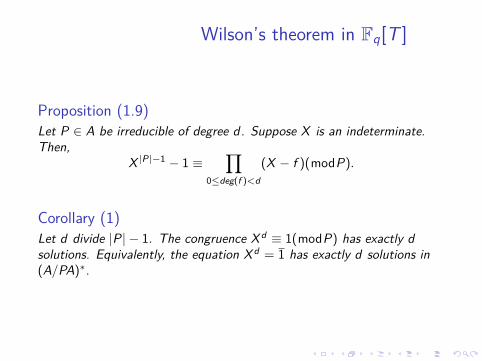
Proposition (1.9)Let P ∈ A be irreducible of degree d. Suppose X is an indeterminate.Then,
X |P|−1 − 1 ≡∏
0≤deg(f )<d
(X − f )(modP).
Corollary (1)Let d divide |P| − 1. The congruence X d ≡ 1(modP) has exactly dsolutions. Equivalently, the equation X d = 1 has exactly d solutions in(A/PA)∗.
Wilson’s theorem in Fq[T ]
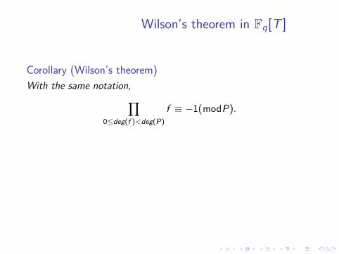
Corollary (Wilson’s theorem)With the same notation,∏
0≤deg(f )<deg(P)
f ≡ −1(modP).
Proof.Just set X = 0 in the proposition. If the characteristic of Fq is oddthen |P| − 1 is even and the result follows. If the characteristic is 2then the result also follows since in characteristic 2 we have−1 = 1.
Wilson’s theorem in Fq[T ]
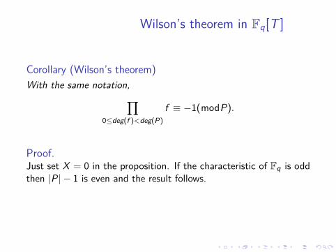
Corollary (Wilson’s theorem)With the same notation,∏
0≤deg(f )<deg(P)
f ≡ −1(modP).
Proof.Just set X = 0 in the proposition. If the characteristic of Fq is oddthen |P| − 1 is even and the result follows.
If the characteristic is 2then the result also follows since in characteristic 2 we have−1 = 1.
Wilson’s theorem in Fq[T ]
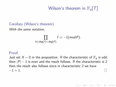
Corollary (Wilson’s theorem)With the same notation,∏
0≤deg(f )<deg(P)
f ≡ −1(modP).
Proof.Just set X = 0 in the proposition. If the characteristic of Fq is oddthen |P| − 1 is even and the result follows. If the characteristic is 2then the result also follows since in characteristic 2 we have−1 = 1.
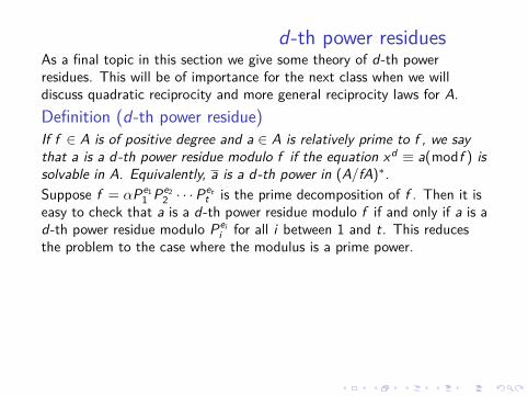
d-th power residuesAs a final topic in this section we give some theory of d-th powerresidues.
This will be of importance for the next class when we willdiscuss quadratic reciprocity and more general reciprocity laws for A.Definition (d-th power residue)If f ∈ A is of positive degree and a ∈ A is relatively prime to f , we saythat a is a d-th power residue modulo f if the equation xd ≡ a(modf ) issolvable in A. Equivalently, a is a d-th power in (A/fA)∗.Suppose f = αPe1
1 Pe22 · · ·P
ett is the prime decomposition of f . Then it is
easy to check that a is a d-th power residue modulo f if and only if a is ad-th power residue modulo Pei
i for all i between 1 and t. This reducesthe problem to the case where the modulus is a prime power.Proposition (1.10)Let P be irreducible and a ∈ A not divisible by P. Assume d divides|P| − 1. The congruence X d ≡ a(modPe) is solvable if and only if
a|P|−1
d ≡ 1(modP).
There are Φ(Pe)d d-th power residues modulo Pe .
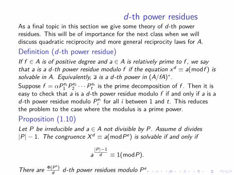
d-th power residuesAs a final topic in this section we give some theory of d-th powerresidues. This will be of importance for the next class when we willdiscuss quadratic reciprocity and more general reciprocity laws for A.
Definition (d-th power residue)If f ∈ A is of positive degree and a ∈ A is relatively prime to f , we saythat a is a d-th power residue modulo f if the equation xd ≡ a(modf ) issolvable in A. Equivalently, a is a d-th power in (A/fA)∗.Suppose f = αPe1
1 Pe22 · · ·P
ett is the prime decomposition of f . Then it is
easy to check that a is a d-th power residue modulo f if and only if a is ad-th power residue modulo Pei
i for all i between 1 and t. This reducesthe problem to the case where the modulus is a prime power.Proposition (1.10)Let P be irreducible and a ∈ A not divisible by P. Assume d divides|P| − 1. The congruence X d ≡ a(modPe) is solvable if and only if
a|P|−1
d ≡ 1(modP).
There are Φ(Pe)d d-th power residues modulo Pe .
d-th power residuesAs a final topic in this section we give some theory of d-th powerresidues. This will be of importance for the next class when we willdiscuss quadratic reciprocity and more general reciprocity laws for A.Definition (d-th power residue)If f ∈ A is of positive degree and a ∈ A is relatively prime to f , we saythat a is a d-th power residue modulo f if the equation xd ≡ a(modf ) issolvable in A.
Equivalently, a is a d-th power in (A/fA)∗.Suppose f = αPe1
1 Pe22 · · ·P
ett is the prime decomposition of f . Then it is
easy to check that a is a d-th power residue modulo f if and only if a is ad-th power residue modulo Pei
i for all i between 1 and t. This reducesthe problem to the case where the modulus is a prime power.Proposition (1.10)Let P be irreducible and a ∈ A not divisible by P. Assume d divides|P| − 1. The congruence X d ≡ a(modPe) is solvable if and only if
a|P|−1
d ≡ 1(modP).
There are Φ(Pe)d d-th power residues modulo Pe .
d-th power residuesAs a final topic in this section we give some theory of d-th powerresidues. This will be of importance for the next class when we willdiscuss quadratic reciprocity and more general reciprocity laws for A.Definition (d-th power residue)If f ∈ A is of positive degree and a ∈ A is relatively prime to f , we saythat a is a d-th power residue modulo f if the equation xd ≡ a(modf ) issolvable in A. Equivalently, a is a d-th power in (A/fA)∗.
Suppose f = αPe11 Pe2
2 · · ·Pett is the prime decomposition of f . Then it is
easy to check that a is a d-th power residue modulo f if and only if a is ad-th power residue modulo Pei
i for all i between 1 and t. This reducesthe problem to the case where the modulus is a prime power.Proposition (1.10)Let P be irreducible and a ∈ A not divisible by P. Assume d divides|P| − 1. The congruence X d ≡ a(modPe) is solvable if and only if
a|P|−1
d ≡ 1(modP).
There are Φ(Pe)d d-th power residues modulo Pe .
d-th power residuesAs a final topic in this section we give some theory of d-th powerresidues. This will be of importance for the next class when we willdiscuss quadratic reciprocity and more general reciprocity laws for A.Definition (d-th power residue)If f ∈ A is of positive degree and a ∈ A is relatively prime to f , we saythat a is a d-th power residue modulo f if the equation xd ≡ a(modf ) issolvable in A. Equivalently, a is a d-th power in (A/fA)∗.Suppose f = αPe1
1 Pe22 · · ·P
ett is the prime decomposition of f . Then it is
easy to check that a is a d-th power residue modulo f if and only if a is ad-th power residue modulo Pei
i for all i between 1 and t. This reducesthe problem to the case where the modulus is a prime power.
Proposition (1.10)Let P be irreducible and a ∈ A not divisible by P. Assume d divides|P| − 1. The congruence X d ≡ a(modPe) is solvable if and only if
a|P|−1
d ≡ 1(modP).
There are Φ(Pe)d d-th power residues modulo Pe .
d-th power residuesAs a final topic in this section we give some theory of d-th powerresidues. This will be of importance for the next class when we willdiscuss quadratic reciprocity and more general reciprocity laws for A.Definition (d-th power residue)If f ∈ A is of positive degree and a ∈ A is relatively prime to f , we saythat a is a d-th power residue modulo f if the equation xd ≡ a(modf ) issolvable in A. Equivalently, a is a d-th power in (A/fA)∗.Suppose f = αPe1
1 Pe22 · · ·P
ett is the prime decomposition of f . Then it is
easy to check that a is a d-th power residue modulo f if and only if a is ad-th power residue modulo Pei
i for all i between 1 and t. This reducesthe problem to the case where the modulus is a prime power.Proposition (1.10)Let P be irreducible and a ∈ A not divisible by P. Assume d divides|P| − 1. The congruence X d ≡ a(modPe) is solvable if and only if
a|P|−1
d ≡ 1(modP).
There are Φ(Pe)d d-th power residues modulo Pe .
Dictionary between Fq[T ] and Z
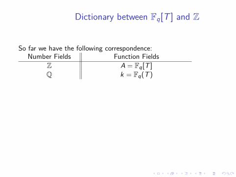
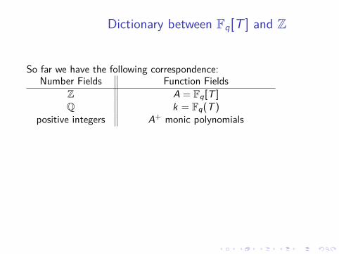
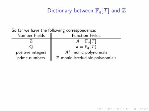
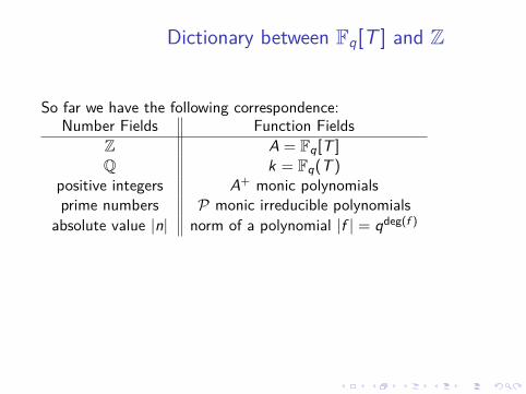
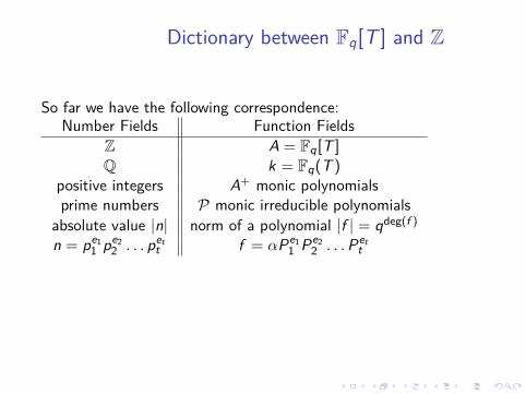
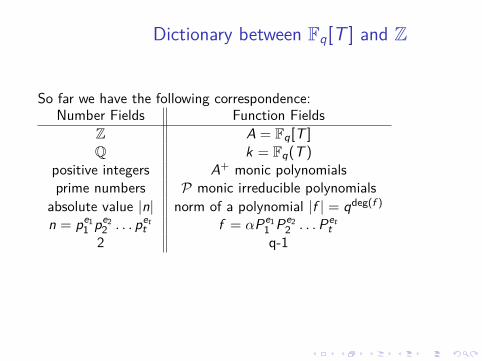
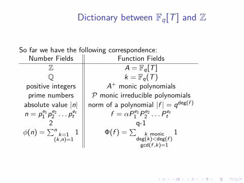
So far we have the following correspondence:
Number Fields Function FieldsZ A = Fq[T ]Q k = Fq(T )
positive integers A+ monic polynomialsprime numbers P monic irreducible polynomials
absolute value |n| norm of a polynomial |f | = qdeg(f )
n = pe11 pe2
2 . . . pett f = αPe1
1 Pe22 . . .Pet
t2 q-1
φ(n) =∑n
k=1(k,n)=1
1 Φ(f ) =∑
k monicdeg(k)<deg(f )
gcd(f ,k)=1
1
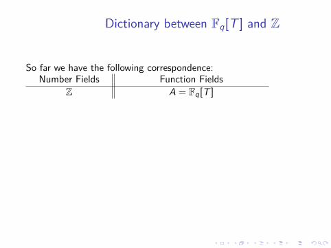
Dictionary between Fq[T ] and Z
So far we have the following correspondence:Number Fields Function Fields
Z A = Fq[T ]
Q k = Fq(T )positive integers A+ monic polynomialsprime numbers P monic irreducible polynomials
absolute value |n| norm of a polynomial |f | = qdeg(f )
n = pe11 pe2
2 . . . pett f = αPe1
1 Pe22 . . .Pet
t2 q-1
φ(n) =∑n
k=1(k,n)=1
1 Φ(f ) =∑
k monicdeg(k)<deg(f )
gcd(f ,k)=1
1
Dictionary between Fq[T ] and Z
So far we have the following correspondence:Number Fields Function Fields
Z A = Fq[T ]Q k = Fq(T )
positive integers A+ monic polynomialsprime numbers P monic irreducible polynomials
absolute value |n| norm of a polynomial |f | = qdeg(f )
n = pe11 pe2
2 . . . pett f = αPe1
1 Pe22 . . .Pet
t2 q-1
φ(n) =∑n
k=1(k,n)=1
1 Φ(f ) =∑
k monicdeg(k)<deg(f )
gcd(f ,k)=1
1
Dictionary between Fq[T ] and Z
So far we have the following correspondence:Number Fields Function Fields
Z A = Fq[T ]Q k = Fq(T )
positive integers A+ monic polynomials
prime numbers P monic irreducible polynomialsabsolute value |n| norm of a polynomial |f | = qdeg(f )
n = pe11 pe2
2 . . . pett f = αPe1
1 Pe22 . . .Pet
t2 q-1
φ(n) =∑n
k=1(k,n)=1
1 Φ(f ) =∑
k monicdeg(k)<deg(f )
gcd(f ,k)=1
1
Dictionary between Fq[T ] and Z
So far we have the following correspondence:Number Fields Function Fields
Z A = Fq[T ]Q k = Fq(T )
positive integers A+ monic polynomialsprime numbers P monic irreducible polynomials
absolute value |n| norm of a polynomial |f | = qdeg(f )
n = pe11 pe2
2 . . . pett f = αPe1
1 Pe22 . . .Pet
t2 q-1
φ(n) =∑n
k=1(k,n)=1
1 Φ(f ) =∑
k monicdeg(k)<deg(f )
gcd(f ,k)=1
1
Dictionary between Fq[T ] and Z
So far we have the following correspondence:Number Fields Function Fields
Z A = Fq[T ]Q k = Fq(T )
positive integers A+ monic polynomialsprime numbers P monic irreducible polynomials
absolute value |n| norm of a polynomial |f | = qdeg(f )
n = pe11 pe2
2 . . . pett f = αPe1
1 Pe22 . . .Pet
t
2 q-1φ(n) =
∑nk=1
(k,n)=11 Φ(f ) =
∑k monic
deg(k)<deg(f )gcd(f ,k)=1
1
Dictionary between Fq[T ] and Z
So far we have the following correspondence:Number Fields Function Fields
Z A = Fq[T ]Q k = Fq(T )
positive integers A+ monic polynomialsprime numbers P monic irreducible polynomials
absolute value |n| norm of a polynomial |f | = qdeg(f )
n = pe11 pe2
2 . . . pett f = αPe1
1 Pe22 . . .Pet
t2 q-1
φ(n) =∑n
k=1(k,n)=1
1 Φ(f ) =∑
k monicdeg(k)<deg(f )
gcd(f ,k)=1
1
Dictionary between Fq[T ] and Z
So far we have the following correspondence:Number Fields Function Fields
Z A = Fq[T ]Q k = Fq(T )
positive integers A+ monic polynomialsprime numbers P monic irreducible polynomials
absolute value |n| norm of a polynomial |f | = qdeg(f )
n = pe11 pe2
2 . . . pett f = αPe1
1 Pe22 . . .Pet
t2 q-1
φ(n) =∑n
k=1(k,n)=1
1 Φ(f ) =∑
k monicdeg(k)<deg(f )
gcd(f ,k)=1
1

Zeta Function and Primes in A = Fq[T ]
• We now discuss properties of primes and prime decompositionin A.
• The discussion will be facilitated by the use of the zetafunction associated to A.
• This zeta function is an analogue of the classical Riemannzeta function ζ(s).
• In A, the zeta function is is a much simpler object. This willlead us to a sharp version of the prime number theorem.
• When we investigate arithmetic in more general function fieldsthan Fq(T ), the corresponding zeta function will turn out tobe a much more subtle invariant.
Zeta Function and Primes in A = Fq[T ]
• We now discuss properties of primes and prime decompositionin A.
• The discussion will be facilitated by the use of the zetafunction associated to A.
• This zeta function is an analogue of the classical Riemannzeta function ζ(s).
• In A, the zeta function is is a much simpler object.
This willlead us to a sharp version of the prime number theorem.
• When we investigate arithmetic in more general function fieldsthan Fq(T ), the corresponding zeta function will turn out tobe a much more subtle invariant.
Zeta Function and Primes in A = Fq[T ]
• We now discuss properties of primes and prime decompositionin A.
• The discussion will be facilitated by the use of the zetafunction associated to A.
• This zeta function is an analogue of the classical Riemannzeta function ζ(s).
• In A, the zeta function is is a much simpler object. This willlead us to a sharp version of the prime number theorem.
• When we investigate arithmetic in more general function fieldsthan Fq(T ), the corresponding zeta function will turn out tobe a much more subtle invariant.
Zeta Function and Primes in A = Fq[T ]
• We now discuss properties of primes and prime decompositionin A.
• The discussion will be facilitated by the use of the zetafunction associated to A.
• This zeta function is an analogue of the classical Riemannzeta function ζ(s).
• In A, the zeta function is is a much simpler object. This willlead us to a sharp version of the prime number theorem.
• When we investigate arithmetic in more general function fieldsthan Fq(T ), the corresponding zeta function will turn out tobe a much more subtle invariant.
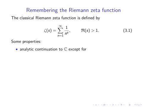
Remembering the Riemann zeta functionThe classical Riemann zeta function is defined by
ζ(s) =∞∑
n=1
1ns , R(s) > 1. (3.1)
Some properties:
• analytic continuation to C except for
• simple pole at s = 1 with residue 1.• Functional Equation. If ξ(s) = π−s/2Γ( s
2 )ζ(s). Then
ξ(s) = ξ(1− s),
where Γ(s) is the classical Gamma function.• ζ(−2n) = 0 for n ∈ Z+. (trivial zeros)
The Riemann Hypothesis: All the non-trivial zeros of ζ(s) havereal part equals 1/2.
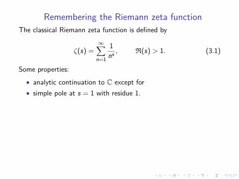
Remembering the Riemann zeta functionThe classical Riemann zeta function is defined by
ζ(s) =∞∑
n=1
1ns , R(s) > 1. (3.1)
Some properties:
• analytic continuation to C except for• simple pole at s = 1 with residue 1.
• Functional Equation. If ξ(s) = π−s/2Γ( s2 )ζ(s). Then
ξ(s) = ξ(1− s),
where Γ(s) is the classical Gamma function.• ζ(−2n) = 0 for n ∈ Z+. (trivial zeros)
The Riemann Hypothesis: All the non-trivial zeros of ζ(s) havereal part equals 1/2.
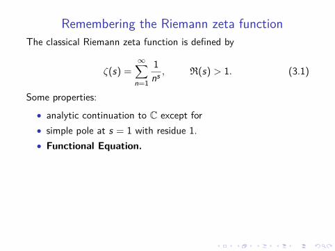
Remembering the Riemann zeta functionThe classical Riemann zeta function is defined by
ζ(s) =∞∑
n=1
1ns , R(s) > 1. (3.1)
Some properties:
• analytic continuation to C except for• simple pole at s = 1 with residue 1.• Functional Equation.
If ξ(s) = π−s/2Γ( s2 )ζ(s). Then
ξ(s) = ξ(1− s),
where Γ(s) is the classical Gamma function.• ζ(−2n) = 0 for n ∈ Z+. (trivial zeros)
The Riemann Hypothesis: All the non-trivial zeros of ζ(s) havereal part equals 1/2.
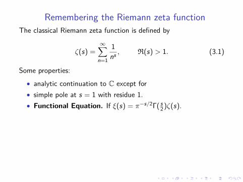
Remembering the Riemann zeta functionThe classical Riemann zeta function is defined by
ζ(s) =∞∑
n=1
1ns , R(s) > 1. (3.1)
Some properties:
• analytic continuation to C except for• simple pole at s = 1 with residue 1.• Functional Equation. If ξ(s) = π−s/2Γ( s
2 )ζ(s).
Then
ξ(s) = ξ(1− s),
where Γ(s) is the classical Gamma function.• ζ(−2n) = 0 for n ∈ Z+. (trivial zeros)
The Riemann Hypothesis: All the non-trivial zeros of ζ(s) havereal part equals 1/2.
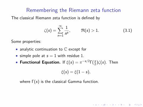
Remembering the Riemann zeta functionThe classical Riemann zeta function is defined by
ζ(s) =∞∑
n=1
1ns , R(s) > 1. (3.1)
Some properties:
• analytic continuation to C except for• simple pole at s = 1 with residue 1.• Functional Equation. If ξ(s) = π−s/2Γ( s
2 )ζ(s). Then
ξ(s) = ξ(1− s),
where Γ(s) is the classical Gamma function.
• ζ(−2n) = 0 for n ∈ Z+. (trivial zeros)
The Riemann Hypothesis: All the non-trivial zeros of ζ(s) havereal part equals 1/2.
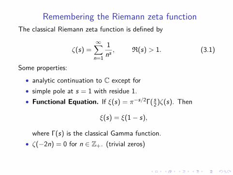
Remembering the Riemann zeta functionThe classical Riemann zeta function is defined by
ζ(s) =∞∑
n=1
1ns , R(s) > 1. (3.1)
Some properties:
• analytic continuation to C except for• simple pole at s = 1 with residue 1.• Functional Equation. If ξ(s) = π−s/2Γ( s
2 )ζ(s). Then
ξ(s) = ξ(1− s),
where Γ(s) is the classical Gamma function.• ζ(−2n) = 0 for n ∈ Z+. (trivial zeros)
The Riemann Hypothesis: All the non-trivial zeros of ζ(s) havereal part equals 1/2.
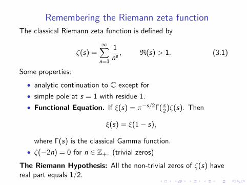
Remembering the Riemann zeta functionThe classical Riemann zeta function is defined by
ζ(s) =∞∑
n=1
1ns , R(s) > 1. (3.1)
Some properties:
• analytic continuation to C except for• simple pole at s = 1 with residue 1.• Functional Equation. If ξ(s) = π−s/2Γ( s
2 )ζ(s). Then
ξ(s) = ξ(1− s),
where Γ(s) is the classical Gamma function.• ζ(−2n) = 0 for n ∈ Z+. (trivial zeros)
The Riemann Hypothesis: All the non-trivial zeros of ζ(s) havereal part equals 1/2.
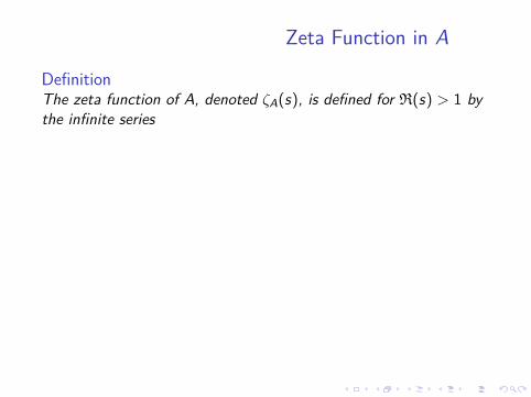
Zeta Function in A
DefinitionThe zeta function of A, denoted ζA(s), is defined for R(s) > 1 bythe infinite series
ζA(s) =∑f ∈A
f monic
1|f |s . (3.2)
There are exactly qd monic polynomials of degree d in A, so onehas
∑deg(f )≤d
|f |−s = 1 +qqs +
q2
q2s + · · ·+ qd
qds ,
and consequentlyζA(s) =
11− q1−s . (3.3)
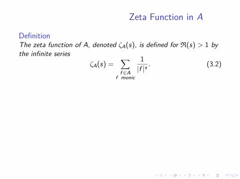
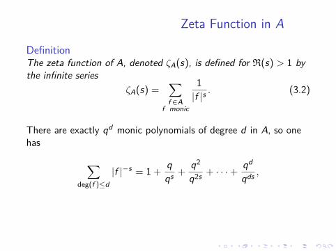
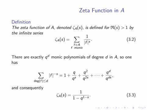
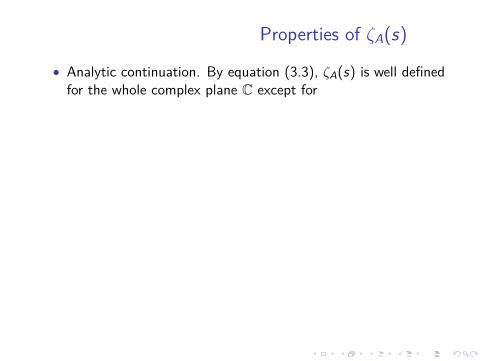
Properties of ζA(s)
• Analytic continuation. By equation (3.3), ζA(s) is well definedfor the whole complex plane C except for
• Simple pole at s = 1 with residue 1log(q) .
• Functional Equation. Let ΓA(s) = (1− q−s)−1 be theGamma function over A. Set ξA(s) = q−sΓA(s)ζA(s). Then itis easy to check that
ξA(s) = ξA(1− s).
As opposed to the case of the classical zeta-function, the proofsare very easy for ζA(s). Later we will consider generalizations ofζA(s) in the context of function fields over finite fields. Similarstatements will hold, but the proofs will be more difficult and willbe based on the Riemann-Roch theorem for algebraic curves.
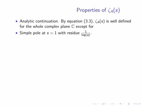
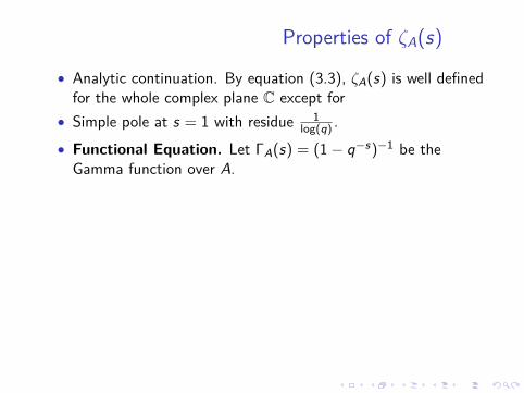
Properties of ζA(s)
• Analytic continuation. By equation (3.3), ζA(s) is well definedfor the whole complex plane C except for
• Simple pole at s = 1 with residue 1log(q) .
• Functional Equation. Let ΓA(s) = (1− q−s)−1 be theGamma function over A.
Set ξA(s) = q−sΓA(s)ζA(s). Then itis easy to check that
ξA(s) = ξA(1− s).
As opposed to the case of the classical zeta-function, the proofsare very easy for ζA(s). Later we will consider generalizations ofζA(s) in the context of function fields over finite fields. Similarstatements will hold, but the proofs will be more difficult and willbe based on the Riemann-Roch theorem for algebraic curves.
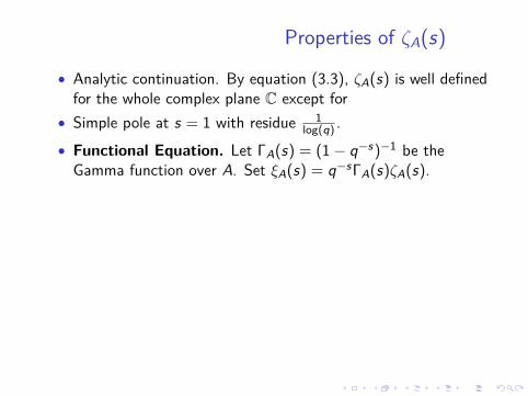
Properties of ζA(s)
• Analytic continuation. By equation (3.3), ζA(s) is well definedfor the whole complex plane C except for
• Simple pole at s = 1 with residue 1log(q) .
• Functional Equation. Let ΓA(s) = (1− q−s)−1 be theGamma function over A. Set ξA(s) = q−sΓA(s)ζA(s).
Then itis easy to check that
ξA(s) = ξA(1− s).
As opposed to the case of the classical zeta-function, the proofsare very easy for ζA(s). Later we will consider generalizations ofζA(s) in the context of function fields over finite fields. Similarstatements will hold, but the proofs will be more difficult and willbe based on the Riemann-Roch theorem for algebraic curves.
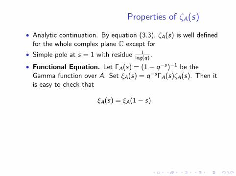
Properties of ζA(s)
• Analytic continuation. By equation (3.3), ζA(s) is well definedfor the whole complex plane C except for
• Simple pole at s = 1 with residue 1log(q) .
• Functional Equation. Let ΓA(s) = (1− q−s)−1 be theGamma function over A. Set ξA(s) = q−sΓA(s)ζA(s). Then itis easy to check that
ξA(s) = ξA(1− s).
As opposed to the case of the classical zeta-function, the proofsare very easy for ζA(s). Later we will consider generalizations ofζA(s) in the context of function fields over finite fields. Similarstatements will hold, but the proofs will be more difficult and willbe based on the Riemann-Roch theorem for algebraic curves.
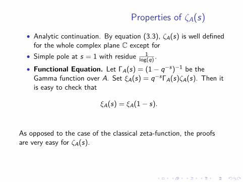
Properties of ζA(s)
• Analytic continuation. By equation (3.3), ζA(s) is well definedfor the whole complex plane C except for
• Simple pole at s = 1 with residue 1log(q) .
• Functional Equation. Let ΓA(s) = (1− q−s)−1 be theGamma function over A. Set ξA(s) = q−sΓA(s)ζA(s). Then itis easy to check that
ξA(s) = ξA(1− s).
As opposed to the case of the classical zeta-function, the proofsare very easy for ζA(s).
Later we will consider generalizations ofζA(s) in the context of function fields over finite fields. Similarstatements will hold, but the proofs will be more difficult and willbe based on the Riemann-Roch theorem for algebraic curves.
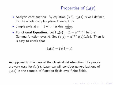
Properties of ζA(s)
• Analytic continuation. By equation (3.3), ζA(s) is well definedfor the whole complex plane C except for
• Simple pole at s = 1 with residue 1log(q) .
• Functional Equation. Let ΓA(s) = (1− q−s)−1 be theGamma function over A. Set ξA(s) = q−sΓA(s)ζA(s). Then itis easy to check that
ξA(s) = ξA(1− s).
As opposed to the case of the classical zeta-function, the proofsare very easy for ζA(s). Later we will consider generalizations ofζA(s) in the context of function fields over finite fields.
Similarstatements will hold, but the proofs will be more difficult and willbe based on the Riemann-Roch theorem for algebraic curves.
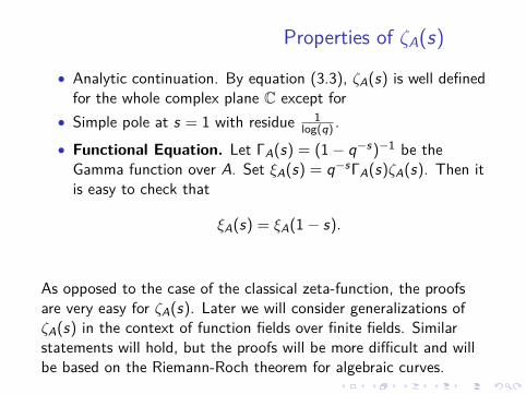
Properties of ζA(s)
• Analytic continuation. By equation (3.3), ζA(s) is well definedfor the whole complex plane C except for
• Simple pole at s = 1 with residue 1log(q) .
• Functional Equation. Let ΓA(s) = (1− q−s)−1 be theGamma function over A. Set ξA(s) = q−sΓA(s)ζA(s). Then itis easy to check that
ξA(s) = ξA(1− s).
As opposed to the case of the classical zeta-function, the proofsare very easy for ζA(s). Later we will consider generalizations ofζA(s) in the context of function fields over finite fields. Similarstatements will hold, but the proofs will be more difficult and willbe based on the Riemann-Roch theorem for algebraic curves.
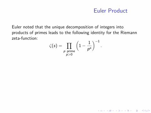
Euler Product
Euler noted that the unique decomposition of integers intoproducts of primes leads to the following identity for the Riemannzeta-function:
ζ(s) =∏
p primep>0
(1− 1
ps
)−1.
This is valid for R(s) > 1. The exact same reasoning (which wewon’t repeat here) leads to the following identity:
ζA(s) =∏
P monicirreducible
(1− 1|P|s
)−1. (3.4)
One can immediately put this Equation in use.
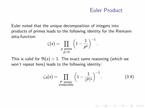
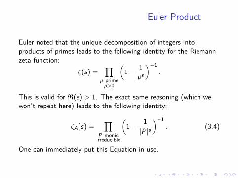
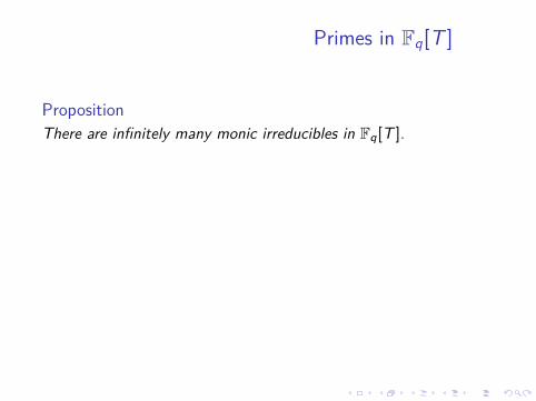
Primes in Fq[T ]
PropositionThere are infinitely many monic irreducibles in Fq[T ].
Proof.Suppose there were only finitely many irreducible polynomials in A.The right-hand side of the Euler product would then be defined ats = 1 and even have a non-zero value there. On the other hand,the left hand side has a pole at s = 1. This shows there areinfinitely many irreducibles in A.One doesn’t need the zeta function to show this. Euclid’s proofthat there are infinitely many prime integers works equally well inA.
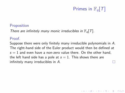
Primes in Fq[T ]
PropositionThere are infinitely many monic irreducibles in Fq[T ].
Proof.Suppose there were only finitely many irreducible polynomials in A.The right-hand side of the Euler product would then be defined ats = 1 and even have a non-zero value there. On the other hand,the left hand side has a pole at s = 1. This shows there areinfinitely many irreducibles in A.
One doesn’t need the zeta function to show this. Euclid’s proofthat there are infinitely many prime integers works equally well inA.
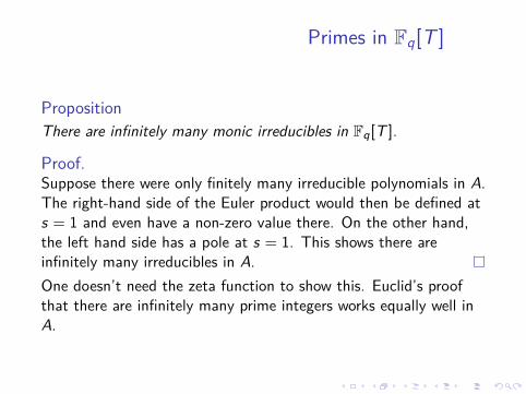
Primes in Fq[T ]
PropositionThere are infinitely many monic irreducibles in Fq[T ].
Proof.Suppose there were only finitely many irreducible polynomials in A.The right-hand side of the Euler product would then be defined ats = 1 and even have a non-zero value there. On the other hand,the left hand side has a pole at s = 1. This shows there areinfinitely many irreducibles in A.One doesn’t need the zeta function to show this. Euclid’s proofthat there are infinitely many prime integers works equally well inA.
Prime Number TheoremLet x be a real number and π(x) be the number of prime numbersless than or equal to x .
Theorem (Prime Number Theorem (1896) - Hadamard and dela Vallee-Poussin)
π(x) ∼ xlog(x)
.
Let d be a positive integer and x = qd . We will show that thenumber of monic irreducibles P such that |P| = x is asymptotic tox/ logq(x) which is clearly in the spirit of the classical result above.Proposition (Gauss)Let ad be the number of monic irreducibles of degree d. Then∑
d |ndad = qn (3.5)
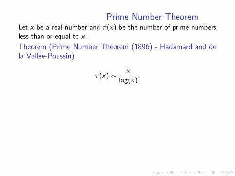
Prime Number TheoremLet x be a real number and π(x) be the number of prime numbersless than or equal to x .Theorem (Prime Number Theorem (1896) - Hadamard and dela Vallee-Poussin)
π(x) ∼ xlog(x)
.
Let d be a positive integer and x = qd . We will show that thenumber of monic irreducibles P such that |P| = x is asymptotic tox/ logq(x) which is clearly in the spirit of the classical result above.Proposition (Gauss)Let ad be the number of monic irreducibles of degree d. Then∑
d |ndad = qn (3.5)
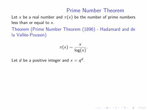
Prime Number TheoremLet x be a real number and π(x) be the number of prime numbersless than or equal to x .Theorem (Prime Number Theorem (1896) - Hadamard and dela Vallee-Poussin)
π(x) ∼ xlog(x)
.
Let d be a positive integer and x = qd .
We will show that thenumber of monic irreducibles P such that |P| = x is asymptotic tox/ logq(x) which is clearly in the spirit of the classical result above.Proposition (Gauss)Let ad be the number of monic irreducibles of degree d. Then∑
d |ndad = qn (3.5)
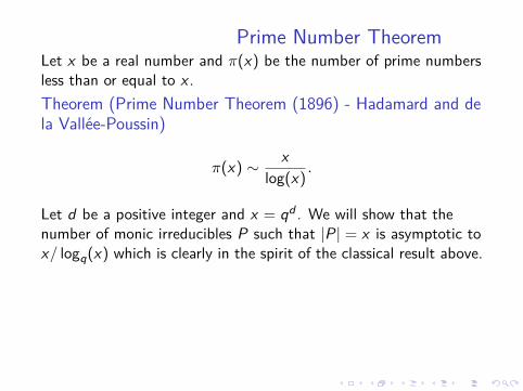
Prime Number TheoremLet x be a real number and π(x) be the number of prime numbersless than or equal to x .Theorem (Prime Number Theorem (1896) - Hadamard and dela Vallee-Poussin)
π(x) ∼ xlog(x)
.
Let d be a positive integer and x = qd . We will show that thenumber of monic irreducibles P such that |P| = x is asymptotic tox/ logq(x) which is clearly in the spirit of the classical result above.
Proposition (Gauss)Let ad be the number of monic irreducibles of degree d. Then∑
d |ndad = qn (3.5)
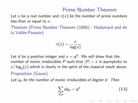
Prime Number TheoremLet x be a real number and π(x) be the number of prime numbersless than or equal to x .Theorem (Prime Number Theorem (1896) - Hadamard and dela Vallee-Poussin)
π(x) ∼ xlog(x)
.
Let d be a positive integer and x = qd . We will show that thenumber of monic irreducibles P such that |P| = x is asymptotic tox/ logq(x) which is clearly in the spirit of the classical result above.Proposition (Gauss)Let ad be the number of monic irreducibles of degree d. Then∑
d |ndad = qn (3.5)
Proof.Define ad to be the number of monic irreducibles of degree d .
Then, from the equation defining ζA(s) we find
ζA(s) =∞∏
d=1(1− q−ds)−ad .
If we recall that ζA(s) = (1− q1−s)−1 and substitute u = q−s
(note that |u| < 1 if and only if R(s) > 1) we obtain the identity
11− qu =
∞∏d=1
(1− ud )−ad .
Taking the logarithmic derivative of both sides and multiplying theresult by u yields
qu1− qu =
∞∑d=1
dad ud
1− ud .
Finally, expand both sides into power series using the geometricseries and compare coefficients of un.
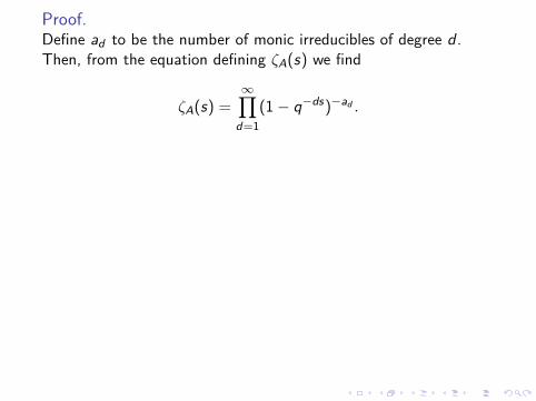
Proof.Define ad to be the number of monic irreducibles of degree d .Then, from the equation defining ζA(s) we find
ζA(s) =∞∏
d=1(1− q−ds)−ad .
If we recall that ζA(s) = (1− q1−s)−1 and substitute u = q−s
(note that |u| < 1 if and only if R(s) > 1) we obtain the identity
11− qu =
∞∏d=1
(1− ud )−ad .
Taking the logarithmic derivative of both sides and multiplying theresult by u yields
qu1− qu =
∞∑d=1
dad ud
1− ud .
Finally, expand both sides into power series using the geometricseries and compare coefficients of un.
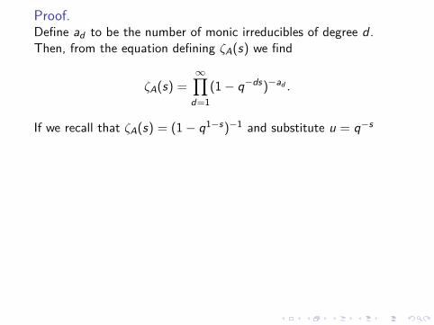
Proof.Define ad to be the number of monic irreducibles of degree d .Then, from the equation defining ζA(s) we find
ζA(s) =∞∏
d=1(1− q−ds)−ad .
If we recall that ζA(s) = (1− q1−s)−1 and substitute u = q−s
(note that |u| < 1 if and only if R(s) > 1) we obtain the identity
11− qu =
∞∏d=1
(1− ud )−ad .
Taking the logarithmic derivative of both sides and multiplying theresult by u yields
qu1− qu =
∞∑d=1
dad ud
1− ud .
Finally, expand both sides into power series using the geometricseries and compare coefficients of un.
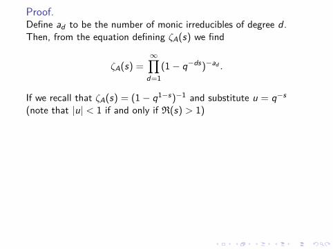
Proof.Define ad to be the number of monic irreducibles of degree d .Then, from the equation defining ζA(s) we find
ζA(s) =∞∏
d=1(1− q−ds)−ad .
If we recall that ζA(s) = (1− q1−s)−1 and substitute u = q−s
(note that |u| < 1 if and only if R(s) > 1)
we obtain the identity
11− qu =
∞∏d=1
(1− ud )−ad .
Taking the logarithmic derivative of both sides and multiplying theresult by u yields
qu1− qu =
∞∑d=1
dad ud
1− ud .
Finally, expand both sides into power series using the geometricseries and compare coefficients of un.
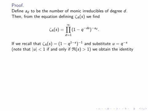
Proof.Define ad to be the number of monic irreducibles of degree d .Then, from the equation defining ζA(s) we find
ζA(s) =∞∏
d=1(1− q−ds)−ad .
If we recall that ζA(s) = (1− q1−s)−1 and substitute u = q−s
(note that |u| < 1 if and only if R(s) > 1) we obtain the identity
11− qu =
∞∏d=1
(1− ud )−ad .
Taking the logarithmic derivative of both sides and multiplying theresult by u yields
qu1− qu =
∞∑d=1
dad ud
1− ud .
Finally, expand both sides into power series using the geometricseries and compare coefficients of un.
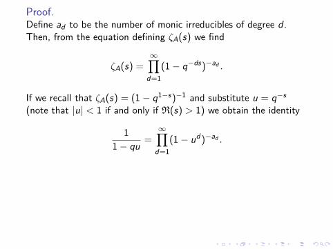
Proof.Define ad to be the number of monic irreducibles of degree d .Then, from the equation defining ζA(s) we find
ζA(s) =∞∏
d=1(1− q−ds)−ad .
If we recall that ζA(s) = (1− q1−s)−1 and substitute u = q−s
(note that |u| < 1 if and only if R(s) > 1) we obtain the identity
11− qu =
∞∏d=1
(1− ud )−ad .
Taking the logarithmic derivative of both sides and multiplying theresult by u yields
qu1− qu =
∞∑d=1
dad ud
1− ud .
Finally, expand both sides into power series using the geometricseries and compare coefficients of un.
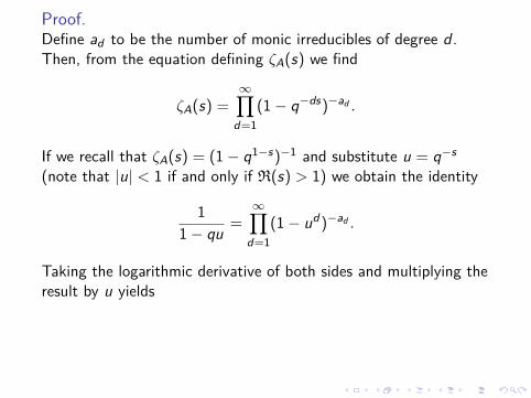
Proof.Define ad to be the number of monic irreducibles of degree d .Then, from the equation defining ζA(s) we find
ζA(s) =∞∏
d=1(1− q−ds)−ad .
If we recall that ζA(s) = (1− q1−s)−1 and substitute u = q−s
(note that |u| < 1 if and only if R(s) > 1) we obtain the identity
11− qu =
∞∏d=1
(1− ud )−ad .
Taking the logarithmic derivative of both sides and multiplying theresult by u yields
qu1− qu =
∞∑d=1
dad ud
1− ud .
Finally, expand both sides into power series using the geometricseries and compare coefficients of un.
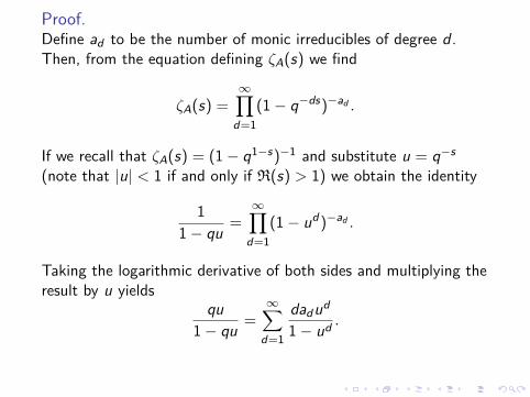
Proof.Define ad to be the number of monic irreducibles of degree d .Then, from the equation defining ζA(s) we find
ζA(s) =∞∏
d=1(1− q−ds)−ad .
If we recall that ζA(s) = (1− q1−s)−1 and substitute u = q−s
(note that |u| < 1 if and only if R(s) > 1) we obtain the identity
11− qu =
∞∏d=1
(1− ud )−ad .
Taking the logarithmic derivative of both sides and multiplying theresult by u yields
qu1− qu =
∞∑d=1
dad ud
1− ud .
Finally, expand both sides into power series using the geometricseries and compare coefficients of un.
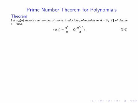
Prime Number Theorem for PolynomialsTheoremLet πA(n) denote the number of monic irreducible polynomials in A = Fq[T ] of degreen. Then,
πA(n) =qn
n+ O(
qn/2
n). (3.6)
Proof.We apply the Mobius inversion formula to the formula given in the proposition toobtain that
an =1n
∑d|n
µ(d)qnd .
From equation above we see that the highest power of q that occurs is qn and thenext highest power that may occur is qn/2 (this occurs if and only if 2 | n). All theother terms have the form ±qm where m ≤ n
3 . The total number of terms is∑d|n |µ(d)|, which is easily seen to be 2t , where t is the number of distinct prime
divisors of n. . Let p1, p2, . . . , pt be the distinct primes dividing n. Then,2t ≤ p1p2 . . . pt ≤ n. Thus, we have the following estimate:∣∣∣an −
qn
n
∣∣∣ ≤ qn/2
n+ qn/3.
Noting that an = πA(n) this establishes the theorem.
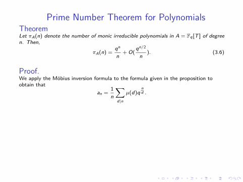
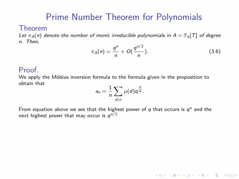
Prime Number Theorem for PolynomialsTheoremLet πA(n) denote the number of monic irreducible polynomials in A = Fq[T ] of degreen. Then,
πA(n) =qn
n+ O(
qn/2
n). (3.6)
Proof.We apply the Mobius inversion formula to the formula given in the proposition toobtain that
an =1n
∑d|n
µ(d)qnd .
From equation above we see that the highest power of q that occurs is qn and thenext highest power that may occur is qn/2
(this occurs if and only if 2 | n). All theother terms have the form ±qm where m ≤ n
3 . The total number of terms is∑d|n |µ(d)|, which is easily seen to be 2t , where t is the number of distinct prime
divisors of n. . Let p1, p2, . . . , pt be the distinct primes dividing n. Then,2t ≤ p1p2 . . . pt ≤ n. Thus, we have the following estimate:∣∣∣an −
qn
n
∣∣∣ ≤ qn/2
n+ qn/3.
Noting that an = πA(n) this establishes the theorem.
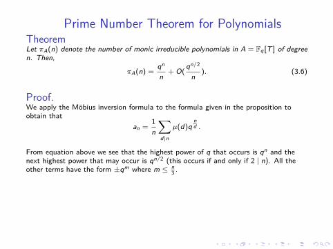
Prime Number Theorem for PolynomialsTheoremLet πA(n) denote the number of monic irreducible polynomials in A = Fq[T ] of degreen. Then,
πA(n) =qn
n+ O(
qn/2
n). (3.6)
Proof.We apply the Mobius inversion formula to the formula given in the proposition toobtain that
an =1n
∑d|n
µ(d)qnd .
From equation above we see that the highest power of q that occurs is qn and thenext highest power that may occur is qn/2 (this occurs if and only if 2 | n). All theother terms have the form ±qm where m ≤ n
3 .
The total number of terms is∑d|n |µ(d)|, which is easily seen to be 2t , where t is the number of distinct prime
divisors of n. . Let p1, p2, . . . , pt be the distinct primes dividing n. Then,2t ≤ p1p2 . . . pt ≤ n. Thus, we have the following estimate:∣∣∣an −
qn
n
∣∣∣ ≤ qn/2
n+ qn/3.
Noting that an = πA(n) this establishes the theorem.
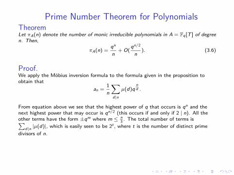
Prime Number Theorem for PolynomialsTheoremLet πA(n) denote the number of monic irreducible polynomials in A = Fq[T ] of degreen. Then,
πA(n) =qn
n+ O(
qn/2
n). (3.6)
Proof.We apply the Mobius inversion formula to the formula given in the proposition toobtain that
an =1n
∑d|n
µ(d)qnd .
From equation above we see that the highest power of q that occurs is qn and thenext highest power that may occur is qn/2 (this occurs if and only if 2 | n). All theother terms have the form ±qm where m ≤ n
3 . The total number of terms is∑d|n |µ(d)|, which is easily seen to be 2t , where t is the number of distinct prime
divisors of n.
. Let p1, p2, . . . , pt be the distinct primes dividing n. Then,2t ≤ p1p2 . . . pt ≤ n. Thus, we have the following estimate:∣∣∣an −
qn
n
∣∣∣ ≤ qn/2
n+ qn/3.
Noting that an = πA(n) this establishes the theorem.
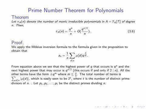
Prime Number Theorem for PolynomialsTheoremLet πA(n) denote the number of monic irreducible polynomials in A = Fq[T ] of degreen. Then,
πA(n) =qn
n+ O(
qn/2
n). (3.6)
Proof.We apply the Mobius inversion formula to the formula given in the proposition toobtain that
an =1n
∑d|n
µ(d)qnd .
From equation above we see that the highest power of q that occurs is qn and thenext highest power that may occur is qn/2 (this occurs if and only if 2 | n). All theother terms have the form ±qm where m ≤ n
3 . The total number of terms is∑d|n |µ(d)|, which is easily seen to be 2t , where t is the number of distinct prime
divisors of n. . Let p1, p2, . . . , pt be the distinct primes dividing n.
Then,2t ≤ p1p2 . . . pt ≤ n. Thus, we have the following estimate:∣∣∣an −
qn
n
∣∣∣ ≤ qn/2
n+ qn/3.
Noting that an = πA(n) this establishes the theorem.
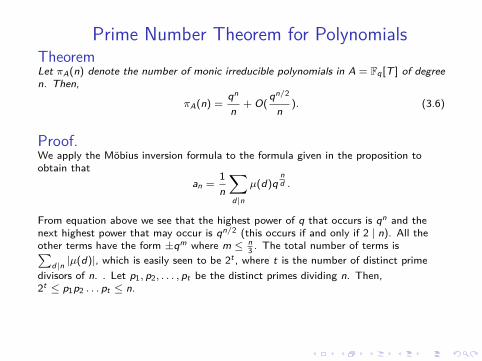
Prime Number Theorem for PolynomialsTheoremLet πA(n) denote the number of monic irreducible polynomials in A = Fq[T ] of degreen. Then,
πA(n) =qn
n+ O(
qn/2
n). (3.6)
Proof.We apply the Mobius inversion formula to the formula given in the proposition toobtain that
an =1n
∑d|n
µ(d)qnd .
From equation above we see that the highest power of q that occurs is qn and thenext highest power that may occur is qn/2 (this occurs if and only if 2 | n). All theother terms have the form ±qm where m ≤ n
3 . The total number of terms is∑d|n |µ(d)|, which is easily seen to be 2t , where t is the number of distinct prime
divisors of n. . Let p1, p2, . . . , pt be the distinct primes dividing n. Then,2t ≤ p1p2 . . . pt ≤ n.
Thus, we have the following estimate:∣∣∣an −qn
n
∣∣∣ ≤ qn/2
n+ qn/3.
Noting that an = πA(n) this establishes the theorem.
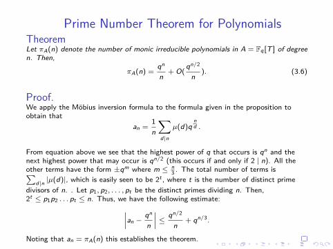
Prime Number Theorem for PolynomialsTheoremLet πA(n) denote the number of monic irreducible polynomials in A = Fq[T ] of degreen. Then,
πA(n) =qn
n+ O(
qn/2
n). (3.6)
Proof.We apply the Mobius inversion formula to the formula given in the proposition toobtain that
an =1n
∑d|n
µ(d)qnd .
From equation above we see that the highest power of q that occurs is qn and thenext highest power that may occur is qn/2 (this occurs if and only if 2 | n). All theother terms have the form ±qm where m ≤ n
3 . The total number of terms is∑d|n |µ(d)|, which is easily seen to be 2t , where t is the number of distinct prime
divisors of n. . Let p1, p2, . . . , pt be the distinct primes dividing n. Then,2t ≤ p1p2 . . . pt ≤ n. Thus, we have the following estimate:∣∣∣an −
qn
n
∣∣∣ ≤ qn/2
n+ qn/3.
Noting that an = πA(n) this establishes the theorem.
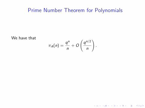
Prime Number Theorem for Polynomials
We have thatπA(n) =
qn
n + O(
qn/2
n
).
Note that if we set x = qn the right-hand side of this equation isx/ logq(x) + O(
√x/ logq(x)) which looks like the conjectured
precise form of the classical prime number theorem. This still notproven. It depends on the truth of the Riemann hypothesis.
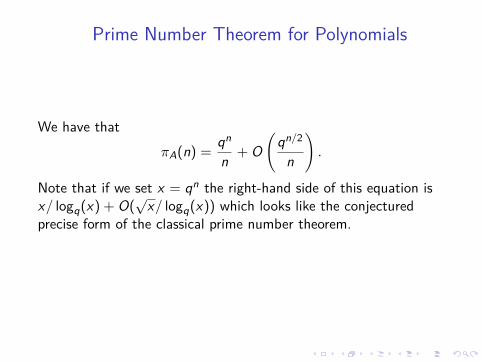
Prime Number Theorem for Polynomials
We have thatπA(n) =
qn
n + O(
qn/2
n
).
Note that if we set x = qn the right-hand side of this equation isx/ logq(x) + O(
√x/ logq(x)) which looks like the conjectured
precise form of the classical prime number theorem.
This still notproven. It depends on the truth of the Riemann hypothesis.
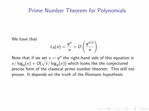
Prime Number Theorem for Polynomials
We have thatπA(n) =
qn
n + O(
qn/2
n
).
Note that if we set x = qn the right-hand side of this equation isx/ logq(x) + O(
√x/ logq(x)) which looks like the conjectured
precise form of the classical prime number theorem. This still notproven. It depends on the truth of the Riemann hypothesis.
The number of square-free polynomialsWe will use the zeta function for other counting problems.
What is the number ofsquare-free monics of degree n?
PropositionLet bn = # {f ∈ A,monic, deg(f ) = n, f square-free}. Then b1 = q and for n > 1,bn = qn(1− q−1).
Proof.Consider the product ∏
P
(1 +
1|P|s
)=∑ δ(f )
|f |s.
As usual, the product is over all monic irreducibles P and the sum is over all monics f .The function δ(f ) is 1 when f is square-free, and 0 otherwise. This is an easyconsequence of unique factorization in A and the definition of square-free. Making thesubstitution u = q−s , the right-hand side of equation above becomes
∑∞n=0 bnun.
Consider the identity 1 + w = (1− w2)/(1− w). If we substitute w = |P|−s and thentake the product over all monic irreducibles P, we see that the left-hand side is equalto ζA(s)/ζA(2s) = (1− q1−2s )/(1− q1−s ). Putting everything in terms of u leads tothe identity
1− qu2
1− qu=
∞∑n=0
bnun.
Expand the left-hand side in a geometric series and compare the coefficients of un.

The number of square-free polynomialsWe will use the zeta function for other counting problems. What is the number ofsquare-free monics of degree n?
PropositionLet bn = # {f ∈ A,monic, deg(f ) = n, f square-free}. Then b1 = q and for n > 1,bn = qn(1− q−1).
Proof.Consider the product ∏
P
(1 +
1|P|s
)=∑ δ(f )
|f |s.
As usual, the product is over all monic irreducibles P and the sum is over all monics f .The function δ(f ) is 1 when f is square-free, and 0 otherwise. This is an easyconsequence of unique factorization in A and the definition of square-free. Making thesubstitution u = q−s , the right-hand side of equation above becomes
∑∞n=0 bnun.
Consider the identity 1 + w = (1− w2)/(1− w). If we substitute w = |P|−s and thentake the product over all monic irreducibles P, we see that the left-hand side is equalto ζA(s)/ζA(2s) = (1− q1−2s )/(1− q1−s ). Putting everything in terms of u leads tothe identity
1− qu2
1− qu=
∞∑n=0
bnun.
Expand the left-hand side in a geometric series and compare the coefficients of un.
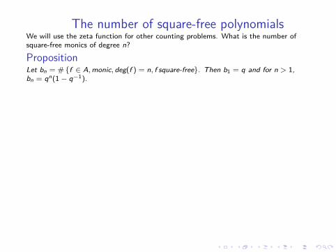
The number of square-free polynomialsWe will use the zeta function for other counting problems. What is the number ofsquare-free monics of degree n?
PropositionLet bn = # {f ∈ A,monic, deg(f ) = n, f square-free}. Then b1 = q and for n > 1,bn = qn(1− q−1).
Proof.Consider the product ∏
P
(1 +
1|P|s
)=∑ δ(f )
|f |s.
As usual, the product is over all monic irreducibles P and the sum is over all monics f .The function δ(f ) is 1 when f is square-free, and 0 otherwise. This is an easyconsequence of unique factorization in A and the definition of square-free. Making thesubstitution u = q−s , the right-hand side of equation above becomes
∑∞n=0 bnun.
Consider the identity 1 + w = (1− w2)/(1− w). If we substitute w = |P|−s and thentake the product over all monic irreducibles P, we see that the left-hand side is equalto ζA(s)/ζA(2s) = (1− q1−2s )/(1− q1−s ). Putting everything in terms of u leads tothe identity
1− qu2
1− qu=
∞∑n=0
bnun.
Expand the left-hand side in a geometric series and compare the coefficients of un.
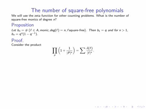
The number of square-free polynomialsWe will use the zeta function for other counting problems. What is the number ofsquare-free monics of degree n?
PropositionLet bn = # {f ∈ A,monic, deg(f ) = n, f square-free}. Then b1 = q and for n > 1,bn = qn(1− q−1).
Proof.Consider the product ∏
P
(1 +
1|P|s
)=∑ δ(f )
|f |s.
As usual, the product is over all monic irreducibles P and the sum is over all monics f .The function δ(f ) is 1 when f is square-free, and 0 otherwise. This is an easyconsequence of unique factorization in A and the definition of square-free. Making thesubstitution u = q−s , the right-hand side of equation above becomes
∑∞n=0 bnun.
Consider the identity 1 + w = (1− w2)/(1− w). If we substitute w = |P|−s and thentake the product over all monic irreducibles P, we see that the left-hand side is equalto ζA(s)/ζA(2s) = (1− q1−2s )/(1− q1−s ). Putting everything in terms of u leads tothe identity
1− qu2
1− qu=
∞∑n=0
bnun.
Expand the left-hand side in a geometric series and compare the coefficients of un.
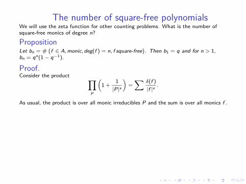
The number of square-free polynomialsWe will use the zeta function for other counting problems. What is the number ofsquare-free monics of degree n?
PropositionLet bn = # {f ∈ A,monic, deg(f ) = n, f square-free}. Then b1 = q and for n > 1,bn = qn(1− q−1).
Proof.Consider the product ∏
P
(1 +
1|P|s
)=∑ δ(f )
|f |s.
As usual, the product is over all monic irreducibles P and the sum is over all monics f .
The function δ(f ) is 1 when f is square-free, and 0 otherwise. This is an easyconsequence of unique factorization in A and the definition of square-free. Making thesubstitution u = q−s , the right-hand side of equation above becomes
∑∞n=0 bnun.
Consider the identity 1 + w = (1− w2)/(1− w). If we substitute w = |P|−s and thentake the product over all monic irreducibles P, we see that the left-hand side is equalto ζA(s)/ζA(2s) = (1− q1−2s )/(1− q1−s ). Putting everything in terms of u leads tothe identity
1− qu2
1− qu=
∞∑n=0
bnun.
Expand the left-hand side in a geometric series and compare the coefficients of un.
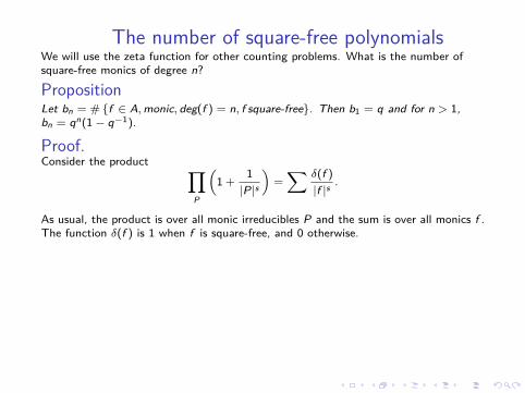
The number of square-free polynomialsWe will use the zeta function for other counting problems. What is the number ofsquare-free monics of degree n?
PropositionLet bn = # {f ∈ A,monic, deg(f ) = n, f square-free}. Then b1 = q and for n > 1,bn = qn(1− q−1).
Proof.Consider the product ∏
P
(1 +
1|P|s
)=∑ δ(f )
|f |s.
As usual, the product is over all monic irreducibles P and the sum is over all monics f .The function δ(f ) is 1 when f is square-free, and 0 otherwise.
This is an easyconsequence of unique factorization in A and the definition of square-free. Making thesubstitution u = q−s , the right-hand side of equation above becomes
∑∞n=0 bnun.
Consider the identity 1 + w = (1− w2)/(1− w). If we substitute w = |P|−s and thentake the product over all monic irreducibles P, we see that the left-hand side is equalto ζA(s)/ζA(2s) = (1− q1−2s )/(1− q1−s ). Putting everything in terms of u leads tothe identity
1− qu2
1− qu=
∞∑n=0
bnun.
Expand the left-hand side in a geometric series and compare the coefficients of un.
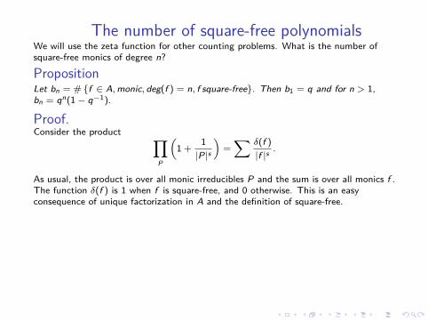
The number of square-free polynomialsWe will use the zeta function for other counting problems. What is the number ofsquare-free monics of degree n?
PropositionLet bn = # {f ∈ A,monic, deg(f ) = n, f square-free}. Then b1 = q and for n > 1,bn = qn(1− q−1).
Proof.Consider the product ∏
P
(1 +
1|P|s
)=∑ δ(f )
|f |s.
As usual, the product is over all monic irreducibles P and the sum is over all monics f .The function δ(f ) is 1 when f is square-free, and 0 otherwise. This is an easyconsequence of unique factorization in A and the definition of square-free.
Making thesubstitution u = q−s , the right-hand side of equation above becomes
∑∞n=0 bnun.
Consider the identity 1 + w = (1− w2)/(1− w). If we substitute w = |P|−s and thentake the product over all monic irreducibles P, we see that the left-hand side is equalto ζA(s)/ζA(2s) = (1− q1−2s )/(1− q1−s ). Putting everything in terms of u leads tothe identity
1− qu2
1− qu=
∞∑n=0
bnun.
Expand the left-hand side in a geometric series and compare the coefficients of un.
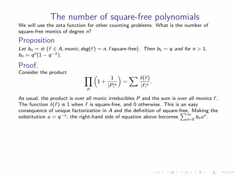
The number of square-free polynomialsWe will use the zeta function for other counting problems. What is the number ofsquare-free monics of degree n?
PropositionLet bn = # {f ∈ A,monic, deg(f ) = n, f square-free}. Then b1 = q and for n > 1,bn = qn(1− q−1).
Proof.Consider the product ∏
P
(1 +
1|P|s
)=∑ δ(f )
|f |s.
As usual, the product is over all monic irreducibles P and the sum is over all monics f .The function δ(f ) is 1 when f is square-free, and 0 otherwise. This is an easyconsequence of unique factorization in A and the definition of square-free. Making thesubstitution u = q−s , the right-hand side of equation above becomes
∑∞n=0 bnun.
Consider the identity 1 + w = (1− w2)/(1− w). If we substitute w = |P|−s and thentake the product over all monic irreducibles P, we see that the left-hand side is equalto ζA(s)/ζA(2s) = (1− q1−2s )/(1− q1−s ). Putting everything in terms of u leads tothe identity
1− qu2
1− qu=
∞∑n=0
bnun.
Expand the left-hand side in a geometric series and compare the coefficients of un.
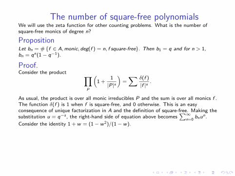
The number of square-free polynomialsWe will use the zeta function for other counting problems. What is the number ofsquare-free monics of degree n?
PropositionLet bn = # {f ∈ A,monic, deg(f ) = n, f square-free}. Then b1 = q and for n > 1,bn = qn(1− q−1).
Proof.Consider the product ∏
P
(1 +
1|P|s
)=∑ δ(f )
|f |s.
As usual, the product is over all monic irreducibles P and the sum is over all monics f .The function δ(f ) is 1 when f is square-free, and 0 otherwise. This is an easyconsequence of unique factorization in A and the definition of square-free. Making thesubstitution u = q−s , the right-hand side of equation above becomes
∑∞n=0 bnun.
Consider the identity 1 + w = (1− w2)/(1− w).
If we substitute w = |P|−s and thentake the product over all monic irreducibles P, we see that the left-hand side is equalto ζA(s)/ζA(2s) = (1− q1−2s )/(1− q1−s ). Putting everything in terms of u leads tothe identity
1− qu2
1− qu=
∞∑n=0
bnun.
Expand the left-hand side in a geometric series and compare the coefficients of un.
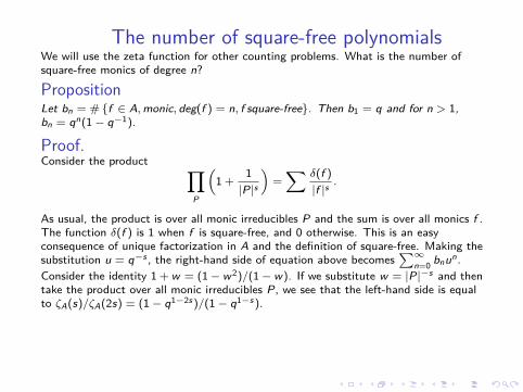
The number of square-free polynomialsWe will use the zeta function for other counting problems. What is the number ofsquare-free monics of degree n?
PropositionLet bn = # {f ∈ A,monic, deg(f ) = n, f square-free}. Then b1 = q and for n > 1,bn = qn(1− q−1).
Proof.Consider the product ∏
P
(1 +
1|P|s
)=∑ δ(f )
|f |s.
As usual, the product is over all monic irreducibles P and the sum is over all monics f .The function δ(f ) is 1 when f is square-free, and 0 otherwise. This is an easyconsequence of unique factorization in A and the definition of square-free. Making thesubstitution u = q−s , the right-hand side of equation above becomes
∑∞n=0 bnun.
Consider the identity 1 + w = (1− w2)/(1− w). If we substitute w = |P|−s and thentake the product over all monic irreducibles P, we see that the left-hand side is equalto ζA(s)/ζA(2s) = (1− q1−2s )/(1− q1−s ).
Putting everything in terms of u leads tothe identity
1− qu2
1− qu=
∞∑n=0
bnun.
Expand the left-hand side in a geometric series and compare the coefficients of un.
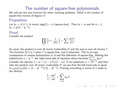
The number of square-free polynomialsWe will use the zeta function for other counting problems. What is the number ofsquare-free monics of degree n?
PropositionLet bn = # {f ∈ A,monic, deg(f ) = n, f square-free}. Then b1 = q and for n > 1,bn = qn(1− q−1).
Proof.Consider the product ∏
P
(1 +
1|P|s
)=∑ δ(f )
|f |s.
As usual, the product is over all monic irreducibles P and the sum is over all monics f .The function δ(f ) is 1 when f is square-free, and 0 otherwise. This is an easyconsequence of unique factorization in A and the definition of square-free. Making thesubstitution u = q−s , the right-hand side of equation above becomes
∑∞n=0 bnun.
Consider the identity 1 + w = (1− w2)/(1− w). If we substitute w = |P|−s and thentake the product over all monic irreducibles P, we see that the left-hand side is equalto ζA(s)/ζA(2s) = (1− q1−2s )/(1− q1−s ). Putting everything in terms of u leads tothe identity
1− qu2
1− qu=
∞∑n=0
bnun.
Expand the left-hand side in a geometric series and compare the coefficients of un.
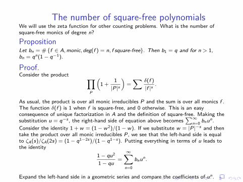
The number of square-free polynomialsWe will use the zeta function for other counting problems. What is the number ofsquare-free monics of degree n?
PropositionLet bn = # {f ∈ A,monic, deg(f ) = n, f square-free}. Then b1 = q and for n > 1,bn = qn(1− q−1).
Proof.Consider the product ∏
P
(1 +
1|P|s
)=∑ δ(f )
|f |s.
As usual, the product is over all monic irreducibles P and the sum is over all monics f .The function δ(f ) is 1 when f is square-free, and 0 otherwise. This is an easyconsequence of unique factorization in A and the definition of square-free. Making thesubstitution u = q−s , the right-hand side of equation above becomes
∑∞n=0 bnun.
Consider the identity 1 + w = (1− w2)/(1− w). If we substitute w = |P|−s and thentake the product over all monic irreducibles P, we see that the left-hand side is equalto ζA(s)/ζA(2s) = (1− q1−2s )/(1− q1−s ). Putting everything in terms of u leads tothe identity
1− qu2
1− qu=
∞∑n=0
bnun.
Expand the left-hand side in a geometric series and compare the coefficients of un.
Let us compare the previous result with what is known to be truein Z.
• Let Bn be the number of positive square-free integers lessthan or equal to n. Then,
limn→∞
Bnn =
6π2 .
• The probability that a positive integer is square-free is 6/π2.• Now the probability that a monic polynomial of degree n is
square-free is bn/qn, and this is equals to (1− q−1) for n > 1.• Thus the probability that a monic polynomial in A is
square-free is (1− q−1) = 1ζA(2) .
• Note that 6/π2 = 1ζ(2)
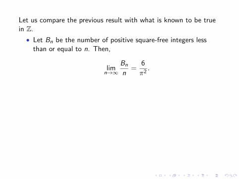
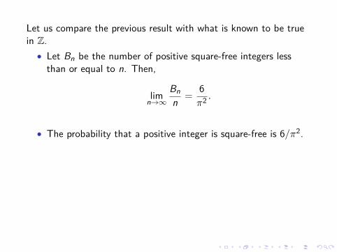
Let us compare the previous result with what is known to be truein Z.
• Let Bn be the number of positive square-free integers lessthan or equal to n. Then,
limn→∞
Bnn =
6π2 .
• The probability that a positive integer is square-free is 6/π2.
• Now the probability that a monic polynomial of degree n issquare-free is bn/qn, and this is equals to (1− q−1) for n > 1.
• Thus the probability that a monic polynomial in A issquare-free is (1− q−1) = 1
ζA(2) .• Note that 6/π2 = 1
ζ(2)
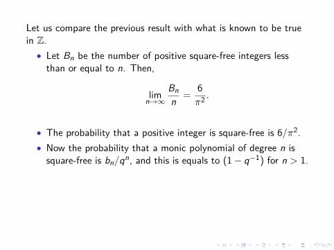
Let us compare the previous result with what is known to be truein Z.
• Let Bn be the number of positive square-free integers lessthan or equal to n. Then,
limn→∞
Bnn =
6π2 .
• The probability that a positive integer is square-free is 6/π2.• Now the probability that a monic polynomial of degree n is
square-free is bn/qn, and this is equals to (1− q−1) for n > 1.
• Thus the probability that a monic polynomial in A issquare-free is (1− q−1) = 1
ζA(2) .• Note that 6/π2 = 1
ζ(2)
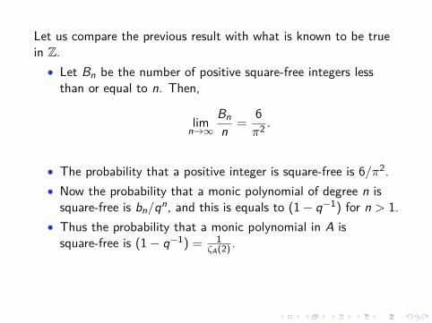
Let us compare the previous result with what is known to be truein Z.
• Let Bn be the number of positive square-free integers lessthan or equal to n. Then,
limn→∞
Bnn =
6π2 .
• The probability that a positive integer is square-free is 6/π2.• Now the probability that a monic polynomial of degree n is
square-free is bn/qn, and this is equals to (1− q−1) for n > 1.• Thus the probability that a monic polynomial in A is
square-free is (1− q−1) = 1ζA(2) .
• Note that 6/π2 = 1ζ(2)
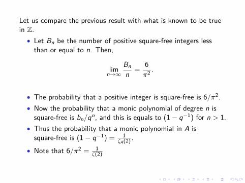
Let us compare the previous result with what is known to be truein Z.
• Let Bn be the number of positive square-free integers lessthan or equal to n. Then,
limn→∞
Bnn =
6π2 .
• The probability that a positive integer is square-free is 6/π2.• Now the probability that a monic polynomial of degree n is
square-free is bn/qn, and this is equals to (1− q−1) for n > 1.• Thus the probability that a monic polynomial in A is
square-free is (1− q−1) = 1ζA(2) .
• Note that 6/π2 = 1ζ(2)
Arithmetic FunctionsOur goal now is to introduce analogues of some well-knownnumber-theoretic functions and to discuss their properties.
We havealready introduced the Euler’s Φ(f ) function.
Definition (Mobius Function)
µ(f ) =
{0 if f is not square-free(−1)t if f = αP1P2 . . .Pt .
(3.7)
Definition (Divisor Functions)Let dk(f ) denote the k-fold divisor function.
dk(f ) =∑
f1...fk =f1,
i.e., dk(f ) is the number of ways to express f as a product of k factors.If k = 2 then d2(f ) = d(f ) is the usual divisor function.
Arithmetic FunctionsOur goal now is to introduce analogues of some well-knownnumber-theoretic functions and to discuss their properties. We havealready introduced the Euler’s Φ(f ) function.
Definition (Mobius Function)
µ(f ) =
{0 if f is not square-free(−1)t if f = αP1P2 . . .Pt .
(3.7)
Definition (Divisor Functions)Let dk(f ) denote the k-fold divisor function.
dk(f ) =∑
f1...fk =f1,
i.e., dk(f ) is the number of ways to express f as a product of k factors.If k = 2 then d2(f ) = d(f ) is the usual divisor function.
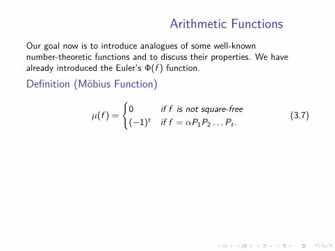
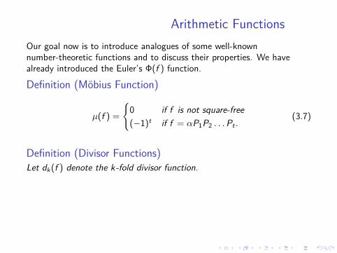
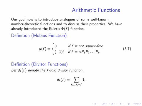
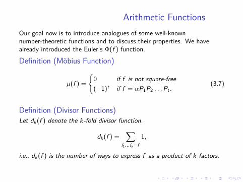
Arithmetic FunctionsOur goal now is to introduce analogues of some well-knownnumber-theoretic functions and to discuss their properties. We havealready introduced the Euler’s Φ(f ) function.
Definition (Mobius Function)
µ(f ) =
{0 if f is not square-free(−1)t if f = αP1P2 . . .Pt .
(3.7)
Definition (Divisor Functions)Let dk(f ) denote the k-fold divisor function.
dk(f ) =∑
f1...fk =f1,
i.e., dk(f ) is the number of ways to express f as a product of k factors.
If k = 2 then d2(f ) = d(f ) is the usual divisor function.
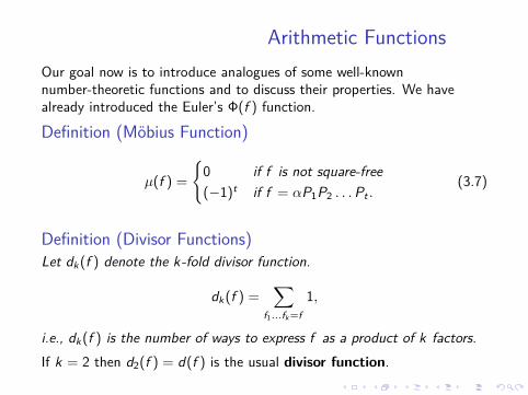
Arithmetic FunctionsOur goal now is to introduce analogues of some well-knownnumber-theoretic functions and to discuss their properties. We havealready introduced the Euler’s Φ(f ) function.
Definition (Mobius Function)
µ(f ) =
{0 if f is not square-free(−1)t if f = αP1P2 . . .Pt .
(3.7)
Definition (Divisor Functions)Let dk(f ) denote the k-fold divisor function.
dk(f ) =∑
f1...fk =f1,
i.e., dk(f ) is the number of ways to express f as a product of k factors.If k = 2 then d2(f ) = d(f ) is the usual divisor function.
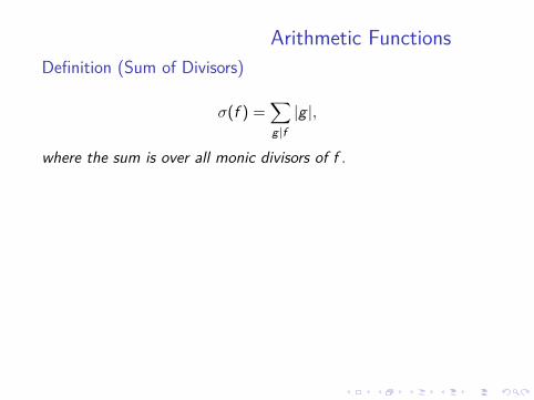
Arithmetic FunctionsDefinition (Sum of Divisors)
σ(f ) =∑g |f|g |,
where the sum is over all monic divisors of f .
Definition (Liouville function)
λ(f ) =
{1 if f = α, α ∈ F∗q(−1)a1+···+ak if f = αPa1
1 Pa22 . . .Pak
k .(3.8)
Note that λ(αf ) = λ(f ).
Definition (von Mangoldt function)
Λ(f ) =
{logq |P| = deg(P) if f = Pk
0 otherwise.(3.9)
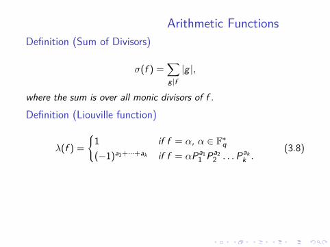
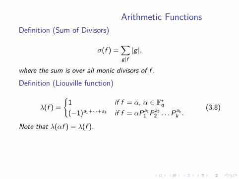
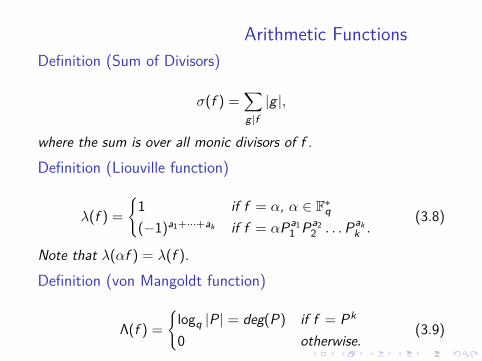
Multiplicative FunctionsSome of these functions, like their counterparts, have the property of beingmultiplicative.
DefinitionA complex valued function F on A− {0} is called multiplicative ifF (fg) = F (f )F (g) whenever f and g are relatively prime. We assume F is 1 onF∗q .Let
f = αPe11 Pe2
2 . . .Pett
be the prime decomposition of f . If F is multiplicative,F (f ) = F (Pe1
1 )F (Pe22 ) . . .F (Pet
t ).
Thus, a multiplicative function is completely determined by its values on primepowers. Using multiplicativity, one can derive the following formulasPropositionLet the prime decomposition of f be given as above. Then,
1 d(f ) = (e1 + 1)(e2 + 1) . . . (et + 1).2
σ(f ) =|P1|e1+1 − 1|P1| − 1
|P2|e2+1 − 1|P2| − 1 · · · |Pt |et +1 − 1
|Pt | − 1 .
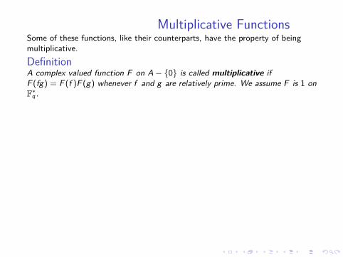
Multiplicative FunctionsSome of these functions, like their counterparts, have the property of beingmultiplicative.DefinitionA complex valued function F on A− {0} is called multiplicative ifF (fg) = F (f )F (g) whenever f and g are relatively prime. We assume F is 1 onF∗q .
Letf = αPe1
1 Pe22 . . .Pet
t
be the prime decomposition of f . If F is multiplicative,F (f ) = F (Pe1
1 )F (Pe22 ) . . .F (Pet
t ).
Thus, a multiplicative function is completely determined by its values on primepowers. Using multiplicativity, one can derive the following formulasPropositionLet the prime decomposition of f be given as above. Then,
1 d(f ) = (e1 + 1)(e2 + 1) . . . (et + 1).2
σ(f ) =|P1|e1+1 − 1|P1| − 1
|P2|e2+1 − 1|P2| − 1 · · · |Pt |et +1 − 1
|Pt | − 1 .
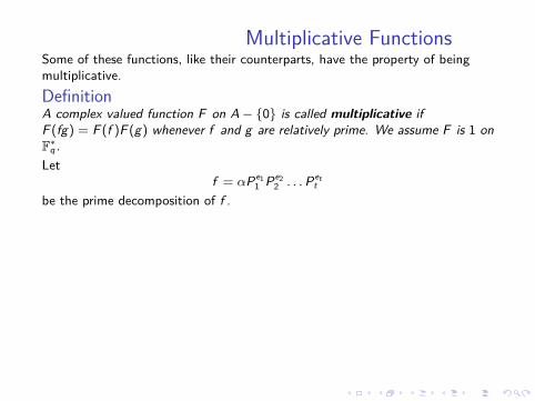
Multiplicative FunctionsSome of these functions, like their counterparts, have the property of beingmultiplicative.DefinitionA complex valued function F on A− {0} is called multiplicative ifF (fg) = F (f )F (g) whenever f and g are relatively prime. We assume F is 1 onF∗q .Let
f = αPe11 Pe2
2 . . .Pett
be the prime decomposition of f .
If F is multiplicative,F (f ) = F (Pe1
1 )F (Pe22 ) . . .F (Pet
t ).
Thus, a multiplicative function is completely determined by its values on primepowers. Using multiplicativity, one can derive the following formulasPropositionLet the prime decomposition of f be given as above. Then,
1 d(f ) = (e1 + 1)(e2 + 1) . . . (et + 1).2
σ(f ) =|P1|e1+1 − 1|P1| − 1
|P2|e2+1 − 1|P2| − 1 · · · |Pt |et +1 − 1
|Pt | − 1 .
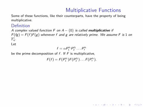
Multiplicative FunctionsSome of these functions, like their counterparts, have the property of beingmultiplicative.DefinitionA complex valued function F on A− {0} is called multiplicative ifF (fg) = F (f )F (g) whenever f and g are relatively prime. We assume F is 1 onF∗q .Let
f = αPe11 Pe2
2 . . .Pett
be the prime decomposition of f . If F is multiplicative,F (f ) = F (Pe1
1 )F (Pe22 ) . . .F (Pet
t ).
Thus, a multiplicative function is completely determined by its values on primepowers. Using multiplicativity, one can derive the following formulasPropositionLet the prime decomposition of f be given as above. Then,
1 d(f ) = (e1 + 1)(e2 + 1) . . . (et + 1).2
σ(f ) =|P1|e1+1 − 1|P1| − 1
|P2|e2+1 − 1|P2| − 1 · · · |Pt |et +1 − 1
|Pt | − 1 .
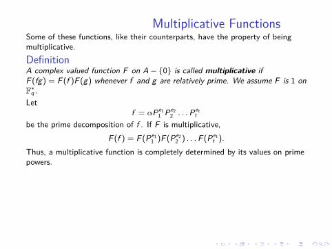
Multiplicative FunctionsSome of these functions, like their counterparts, have the property of beingmultiplicative.DefinitionA complex valued function F on A− {0} is called multiplicative ifF (fg) = F (f )F (g) whenever f and g are relatively prime. We assume F is 1 onF∗q .Let
f = αPe11 Pe2
2 . . .Pett
be the prime decomposition of f . If F is multiplicative,F (f ) = F (Pe1
1 )F (Pe22 ) . . .F (Pet
t ).
Thus, a multiplicative function is completely determined by its values on primepowers.
Using multiplicativity, one can derive the following formulasPropositionLet the prime decomposition of f be given as above. Then,
1 d(f ) = (e1 + 1)(e2 + 1) . . . (et + 1).2
σ(f ) =|P1|e1+1 − 1|P1| − 1
|P2|e2+1 − 1|P2| − 1 · · · |Pt |et +1 − 1
|Pt | − 1 .
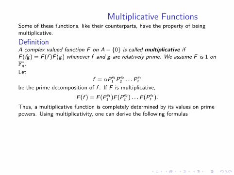
Multiplicative FunctionsSome of these functions, like their counterparts, have the property of beingmultiplicative.DefinitionA complex valued function F on A− {0} is called multiplicative ifF (fg) = F (f )F (g) whenever f and g are relatively prime. We assume F is 1 onF∗q .Let
f = αPe11 Pe2
2 . . .Pett
be the prime decomposition of f . If F is multiplicative,F (f ) = F (Pe1
1 )F (Pe22 ) . . .F (Pet
t ).
Thus, a multiplicative function is completely determined by its values on primepowers. Using multiplicativity, one can derive the following formulas
PropositionLet the prime decomposition of f be given as above. Then,
1 d(f ) = (e1 + 1)(e2 + 1) . . . (et + 1).2
σ(f ) =|P1|e1+1 − 1|P1| − 1
|P2|e2+1 − 1|P2| − 1 · · · |Pt |et +1 − 1
|Pt | − 1 .
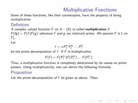
Multiplicative FunctionsSome of these functions, like their counterparts, have the property of beingmultiplicative.DefinitionA complex valued function F on A− {0} is called multiplicative ifF (fg) = F (f )F (g) whenever f and g are relatively prime. We assume F is 1 onF∗q .Let
f = αPe11 Pe2
2 . . .Pett
be the prime decomposition of f . If F is multiplicative,F (f ) = F (Pe1
1 )F (Pe22 ) . . .F (Pet
t ).
Thus, a multiplicative function is completely determined by its values on primepowers. Using multiplicativity, one can derive the following formulasPropositionLet the prime decomposition of f be given as above. Then,
1 d(f ) = (e1 + 1)(e2 + 1) . . . (et + 1).2
σ(f ) =|P1|e1+1 − 1|P1| − 1
|P2|e2+1 − 1|P2| − 1 · · · |Pt |et +1 − 1
|Pt | − 1 .
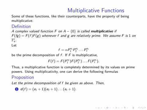
Multiplicative FunctionsSome of these functions, like their counterparts, have the property of beingmultiplicative.DefinitionA complex valued function F on A− {0} is called multiplicative ifF (fg) = F (f )F (g) whenever f and g are relatively prime. We assume F is 1 onF∗q .Let
f = αPe11 Pe2
2 . . .Pett
be the prime decomposition of f . If F is multiplicative,F (f ) = F (Pe1
1 )F (Pe22 ) . . .F (Pet
t ).
Thus, a multiplicative function is completely determined by its values on primepowers. Using multiplicativity, one can derive the following formulasPropositionLet the prime decomposition of f be given as above. Then,
1 d(f ) = (e1 + 1)(e2 + 1) . . . (et + 1).
2
σ(f ) =|P1|e1+1 − 1|P1| − 1
|P2|e2+1 − 1|P2| − 1 · · · |Pt |et +1 − 1
|Pt | − 1 .
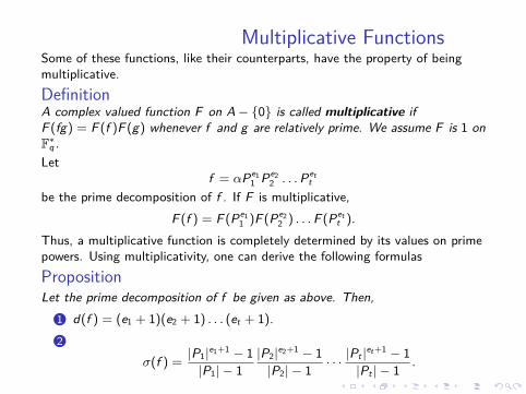
Multiplicative FunctionsSome of these functions, like their counterparts, have the property of beingmultiplicative.DefinitionA complex valued function F on A− {0} is called multiplicative ifF (fg) = F (f )F (g) whenever f and g are relatively prime. We assume F is 1 onF∗q .Let
f = αPe11 Pe2
2 . . .Pett
be the prime decomposition of f . If F is multiplicative,F (f ) = F (Pe1
1 )F (Pe22 ) . . .F (Pet
t ).
Thus, a multiplicative function is completely determined by its values on primepowers. Using multiplicativity, one can derive the following formulasPropositionLet the prime decomposition of f be given as above. Then,
1 d(f ) = (e1 + 1)(e2 + 1) . . . (et + 1).2
σ(f ) =|P1|e1+1 − 1|P1| − 1
|P2|e2+1 − 1|P2| − 1 · · · |Pt |et +1 − 1
|Pt | − 1 .
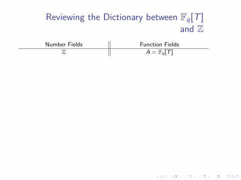
Reviewing the Dictionary between Fq[T ]and Z
Number Fields Function FieldsZ A = Fq[T ]
Q k = Fq(T )positive integers A+ monic polynomialsprime numbers P monic irreducible polynomials
absolute value |n| norm of a polynomial |f | = qdeg(f )
n = pe11 pe2
2 . . . pett f = αPe1
1 Pe2...Pett
22 q-1
φ(n) =∑n
k=1(k,n)=1
1 Φ(f ) =∑
k monicdeg(k)<deg(f )
gcd(f ,k)=1
1
n = pe11 . . . pet
t f = αPe11 . . .Pet
tζ(s) =
∑∞n=1
1ns ζA(s) =
∑f monic
1|f |s
ξ(s) = π−s2 Γ( s
2 )ζ(s) = ξ(1− s) ξA(s) = q−sΓA(s)ζA(s) = ξA(1− s)ζ(s) has analytic continuation ζA(s) = (1− q1−s)−1
π(x) ∼ xlog(x)
πA(n) = qn
n + O( qn/2
n )
µ(n), dk (n), ϕ(n),Λ(n), λ(n) µ(f ), dk (f ),Φ(f ),Λ(f ), λ(f )
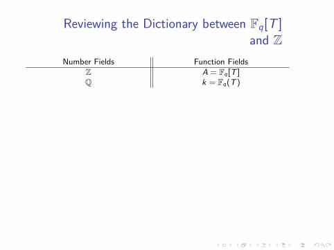
Reviewing the Dictionary between Fq[T ]and Z
Number Fields Function FieldsZ A = Fq[T ]Q k = Fq(T )
positive integers A+ monic polynomialsprime numbers P monic irreducible polynomials
absolute value |n| norm of a polynomial |f | = qdeg(f )
n = pe11 pe2
2 . . . pett f = αPe1
1 Pe2...Pett
22 q-1
φ(n) =∑n
k=1(k,n)=1
1 Φ(f ) =∑
k monicdeg(k)<deg(f )
gcd(f ,k)=1
1
n = pe11 . . . pet
t f = αPe11 . . .Pet
tζ(s) =
∑∞n=1
1ns ζA(s) =
∑f monic
1|f |s
ξ(s) = π−s2 Γ( s
2 )ζ(s) = ξ(1− s) ξA(s) = q−sΓA(s)ζA(s) = ξA(1− s)ζ(s) has analytic continuation ζA(s) = (1− q1−s)−1
π(x) ∼ xlog(x)
πA(n) = qn
n + O( qn/2
n )
µ(n), dk (n), ϕ(n),Λ(n), λ(n) µ(f ), dk (f ),Φ(f ),Λ(f ), λ(f )
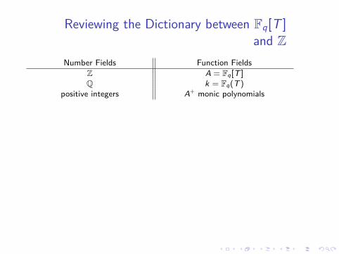
Reviewing the Dictionary between Fq[T ]and Z
Number Fields Function FieldsZ A = Fq[T ]Q k = Fq(T )
positive integers A+ monic polynomials
prime numbers P monic irreducible polynomialsabsolute value |n| norm of a polynomial |f | = qdeg(f )
n = pe11 pe2
2 . . . pett f = αPe1
1 Pe2...Pett
22 q-1
φ(n) =∑n
k=1(k,n)=1
1 Φ(f ) =∑
k monicdeg(k)<deg(f )
gcd(f ,k)=1
1
n = pe11 . . . pet
t f = αPe11 . . .Pet
tζ(s) =
∑∞n=1
1ns ζA(s) =
∑f monic
1|f |s
ξ(s) = π−s2 Γ( s
2 )ζ(s) = ξ(1− s) ξA(s) = q−sΓA(s)ζA(s) = ξA(1− s)ζ(s) has analytic continuation ζA(s) = (1− q1−s)−1
π(x) ∼ xlog(x)
πA(n) = qn
n + O( qn/2
n )
µ(n), dk (n), ϕ(n),Λ(n), λ(n) µ(f ), dk (f ),Φ(f ),Λ(f ), λ(f )
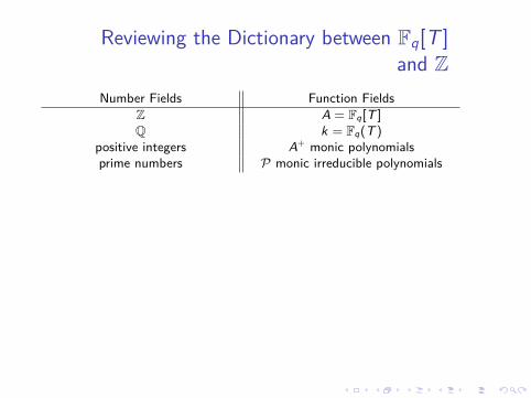
Reviewing the Dictionary between Fq[T ]and Z
Number Fields Function FieldsZ A = Fq[T ]Q k = Fq(T )
positive integers A+ monic polynomialsprime numbers P monic irreducible polynomials
absolute value |n| norm of a polynomial |f | = qdeg(f )
n = pe11 pe2
2 . . . pett f = αPe1
1 Pe2...Pett
22 q-1
φ(n) =∑n
k=1(k,n)=1
1 Φ(f ) =∑
k monicdeg(k)<deg(f )
gcd(f ,k)=1
1
n = pe11 . . . pet
t f = αPe11 . . .Pet
tζ(s) =
∑∞n=1
1ns ζA(s) =
∑f monic
1|f |s
ξ(s) = π−s2 Γ( s
2 )ζ(s) = ξ(1− s) ξA(s) = q−sΓA(s)ζA(s) = ξA(1− s)ζ(s) has analytic continuation ζA(s) = (1− q1−s)−1
π(x) ∼ xlog(x)
πA(n) = qn
n + O( qn/2
n )
µ(n), dk (n), ϕ(n),Λ(n), λ(n) µ(f ), dk (f ),Φ(f ),Λ(f ), λ(f )
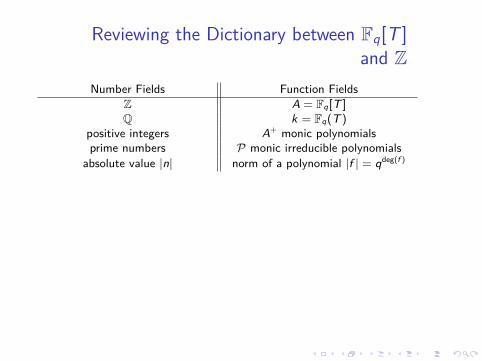
Reviewing the Dictionary between Fq[T ]and Z
Number Fields Function FieldsZ A = Fq[T ]Q k = Fq(T )
positive integers A+ monic polynomialsprime numbers P monic irreducible polynomials
absolute value |n| norm of a polynomial |f | = qdeg(f )
n = pe11 pe2
2 . . . pett f = αPe1
1 Pe2...Pett
2
2 q-1φ(n) =
∑nk=1
(k,n)=11 Φ(f ) =
∑k monic
deg(k)<deg(f )gcd(f ,k)=1
1
n = pe11 . . . pet
t f = αPe11 . . .Pet
tζ(s) =
∑∞n=1
1ns ζA(s) =
∑f monic
1|f |s
ξ(s) = π−s2 Γ( s
2 )ζ(s) = ξ(1− s) ξA(s) = q−sΓA(s)ζA(s) = ξA(1− s)ζ(s) has analytic continuation ζA(s) = (1− q1−s)−1
π(x) ∼ xlog(x)
πA(n) = qn
n + O( qn/2
n )
µ(n), dk (n), ϕ(n),Λ(n), λ(n) µ(f ), dk (f ),Φ(f ),Λ(f ), λ(f )
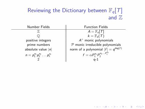
Reviewing the Dictionary between Fq[T ]and Z
Number Fields Function FieldsZ A = Fq[T ]Q k = Fq(T )
positive integers A+ monic polynomialsprime numbers P monic irreducible polynomials
absolute value |n| norm of a polynomial |f | = qdeg(f )
n = pe11 pe2
2 . . . pett f = αPe1
1 Pe2...Pett
22 q-1
φ(n) =∑n
k=1(k,n)=1
1 Φ(f ) =∑
k monicdeg(k)<deg(f )
gcd(f ,k)=1
1
n = pe11 . . . pet
t f = αPe11 . . .Pet
tζ(s) =
∑∞n=1
1ns ζA(s) =
∑f monic
1|f |s
ξ(s) = π−s2 Γ( s
2 )ζ(s) = ξ(1− s) ξA(s) = q−sΓA(s)ζA(s) = ξA(1− s)ζ(s) has analytic continuation ζA(s) = (1− q1−s)−1
π(x) ∼ xlog(x)
πA(n) = qn
n + O( qn/2
n )
µ(n), dk (n), ϕ(n),Λ(n), λ(n) µ(f ), dk (f ),Φ(f ),Λ(f ), λ(f )
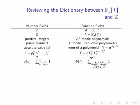
Reviewing the Dictionary between Fq[T ]and Z
Number Fields Function FieldsZ A = Fq[T ]Q k = Fq(T )
positive integers A+ monic polynomialsprime numbers P monic irreducible polynomials
absolute value |n| norm of a polynomial |f | = qdeg(f )
n = pe11 pe2
2 . . . pett f = αPe1
1 Pe2...Pett
22 q-1
φ(n) =∑n
k=1(k,n)=1
1 Φ(f ) =∑
k monicdeg(k)<deg(f )
gcd(f ,k)=1
1
n = pe11 . . . pet
t f = αPe11 . . .Pet
tζ(s) =
∑∞n=1
1ns ζA(s) =
∑f monic
1|f |s
ξ(s) = π−s2 Γ( s
2 )ζ(s) = ξ(1− s) ξA(s) = q−sΓA(s)ζA(s) = ξA(1− s)ζ(s) has analytic continuation ζA(s) = (1− q1−s)−1
π(x) ∼ xlog(x)
πA(n) = qn
n + O( qn/2
n )
µ(n), dk (n), ϕ(n),Λ(n), λ(n) µ(f ), dk (f ),Φ(f ),Λ(f ), λ(f )
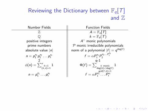
Reviewing the Dictionary between Fq[T ]and Z
Number Fields Function FieldsZ A = Fq[T ]Q k = Fq(T )
positive integers A+ monic polynomialsprime numbers P monic irreducible polynomials
absolute value |n| norm of a polynomial |f | = qdeg(f )
n = pe11 pe2
2 . . . pett f = αPe1
1 Pe2...Pett
22 q-1
φ(n) =∑n
k=1(k,n)=1
1 Φ(f ) =∑
k monicdeg(k)<deg(f )
gcd(f ,k)=1
1
n = pe11 . . . pet
t f = αPe11 . . .Pet
t
ζ(s) =∑∞
n=11ns ζA(s) =
∑f monic
1|f |s
ξ(s) = π−s2 Γ( s
2 )ζ(s) = ξ(1− s) ξA(s) = q−sΓA(s)ζA(s) = ξA(1− s)ζ(s) has analytic continuation ζA(s) = (1− q1−s)−1
π(x) ∼ xlog(x)
πA(n) = qn
n + O( qn/2
n )
µ(n), dk (n), ϕ(n),Λ(n), λ(n) µ(f ), dk (f ),Φ(f ),Λ(f ), λ(f )
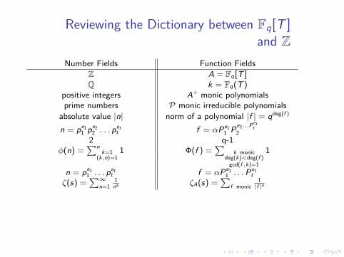
Reviewing the Dictionary between Fq[T ]and Z
Number Fields Function FieldsZ A = Fq[T ]Q k = Fq(T )
positive integers A+ monic polynomialsprime numbers P monic irreducible polynomials
absolute value |n| norm of a polynomial |f | = qdeg(f )
n = pe11 pe2
2 . . . pett f = αPe1
1 Pe2...Pett
22 q-1
φ(n) =∑n
k=1(k,n)=1
1 Φ(f ) =∑
k monicdeg(k)<deg(f )
gcd(f ,k)=1
1
n = pe11 . . . pet
t f = αPe11 . . .Pet
tζ(s) =
∑∞n=1
1ns ζA(s) =
∑f monic
1|f |s
ξ(s) = π−s2 Γ( s
2 )ζ(s) = ξ(1− s) ξA(s) = q−sΓA(s)ζA(s) = ξA(1− s)ζ(s) has analytic continuation ζA(s) = (1− q1−s)−1
π(x) ∼ xlog(x)
πA(n) = qn
n + O( qn/2
n )
µ(n), dk (n), ϕ(n),Λ(n), λ(n) µ(f ), dk (f ),Φ(f ),Λ(f ), λ(f )
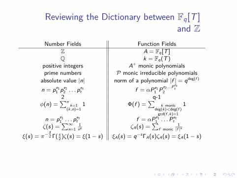
Reviewing the Dictionary between Fq[T ]and Z
Number Fields Function FieldsZ A = Fq[T ]Q k = Fq(T )
positive integers A+ monic polynomialsprime numbers P monic irreducible polynomials
absolute value |n| norm of a polynomial |f | = qdeg(f )
n = pe11 pe2
2 . . . pett f = αPe1
1 Pe2...Pett
22 q-1
φ(n) =∑n
k=1(k,n)=1
1 Φ(f ) =∑
k monicdeg(k)<deg(f )
gcd(f ,k)=1
1
n = pe11 . . . pet
t f = αPe11 . . .Pet
tζ(s) =
∑∞n=1
1ns ζA(s) =
∑f monic
1|f |s
ξ(s) = π−s2 Γ( s
2 )ζ(s) = ξ(1− s) ξA(s) = q−sΓA(s)ζA(s) = ξA(1− s)
ζ(s) has analytic continuation ζA(s) = (1− q1−s)−1
π(x) ∼ xlog(x)
πA(n) = qn
n + O( qn/2
n )
µ(n), dk (n), ϕ(n),Λ(n), λ(n) µ(f ), dk (f ),Φ(f ),Λ(f ), λ(f )
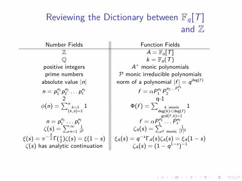
Reviewing the Dictionary between Fq[T ]and Z
Number Fields Function FieldsZ A = Fq[T ]Q k = Fq(T )
positive integers A+ monic polynomialsprime numbers P monic irreducible polynomials
absolute value |n| norm of a polynomial |f | = qdeg(f )
n = pe11 pe2
2 . . . pett f = αPe1
1 Pe2...Pett
22 q-1
φ(n) =∑n
k=1(k,n)=1
1 Φ(f ) =∑
k monicdeg(k)<deg(f )
gcd(f ,k)=1
1
n = pe11 . . . pet
t f = αPe11 . . .Pet
tζ(s) =
∑∞n=1
1ns ζA(s) =
∑f monic
1|f |s
ξ(s) = π−s2 Γ( s
2 )ζ(s) = ξ(1− s) ξA(s) = q−sΓA(s)ζA(s) = ξA(1− s)ζ(s) has analytic continuation ζA(s) = (1− q1−s)−1
π(x) ∼ xlog(x)
πA(n) = qn
n + O( qn/2
n )
µ(n), dk (n), ϕ(n),Λ(n), λ(n) µ(f ), dk (f ),Φ(f ),Λ(f ), λ(f )
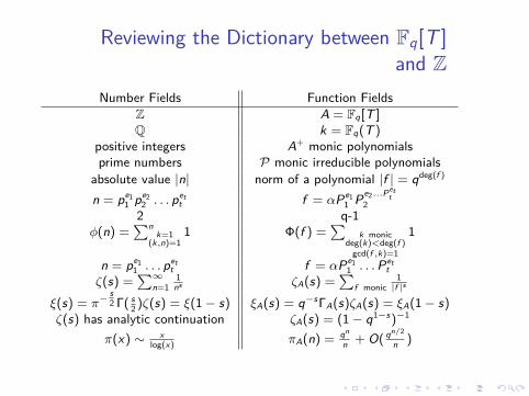
Reviewing the Dictionary between Fq[T ]and Z
Number Fields Function FieldsZ A = Fq[T ]Q k = Fq(T )
positive integers A+ monic polynomialsprime numbers P monic irreducible polynomials
absolute value |n| norm of a polynomial |f | = qdeg(f )
n = pe11 pe2
2 . . . pett f = αPe1
1 Pe2...Pett
22 q-1
φ(n) =∑n
k=1(k,n)=1
1 Φ(f ) =∑
k monicdeg(k)<deg(f )
gcd(f ,k)=1
1
n = pe11 . . . pet
t f = αPe11 . . .Pet
tζ(s) =
∑∞n=1
1ns ζA(s) =
∑f monic
1|f |s
ξ(s) = π−s2 Γ( s
2 )ζ(s) = ξ(1− s) ξA(s) = q−sΓA(s)ζA(s) = ξA(1− s)ζ(s) has analytic continuation ζA(s) = (1− q1−s)−1
π(x) ∼ xlog(x)
πA(n) = qn
n + O( qn/2
n )
µ(n), dk (n), ϕ(n),Λ(n), λ(n) µ(f ), dk (f ),Φ(f ),Λ(f ), λ(f )