and the role of taxation- oecd economics department

OECD Economics Department Working Papers No. 713

Economic Growthand the Role of Taxation-

TheoryGareth D. Myles

https://dx.doi.org/10.1787/222800633678

https://dx.doi.org/10.1787/222800633678

Unclassified ECO/WKP(2009)54 Organisation de Coopération et de Développement Économiques Organisation for Economic Co-operation and Development 15-Jul-2009 ________________________________________________________________________________________________________ English - Or. English ECONOMICS DEPARTMENT

ECONOMIC GROWTH AND THE ROLE OF TAXATION - THEORY ECONOMICS DEPARTMENT WORKING PAPERS NO.713

By Gareth D. Myles University of Exeter and Institute for Fiscal Studies

All Economics Department Working Papers are available through OECD's internet web site at www.oecd.org/eco/working_papers

JT03267978 Document complet disponible sur OLIS dans son format d'origine Complete document available on OLIS in its original format

EC

O/W

KP

(2009)54 U

nclassified

English - O

r. English

ECO/WKP(2009)54

2

ABSTRACT/RESUMÉ

Economic growth and the role of taxation – Theory

Economic growth is the basis of increased prosperity. This makes the attainment of growth a key objective for governments across the world. The rate of growth can be affected by policy choices through the effect that taxation has upon economic decisions and through productive public expenditures. This paper provides a self-contained introduction to the economic modelling of growth and reviews the theoretical evidence on the extent of the link between taxation and growth.

JEL Classification: O4; H2, H3 Keywords: Economic growth; taxation; public policy.

++++++++++++++++++++++

La croissance économique et le rôle de la fiscalité - Théorie

La croissance économique est au fondement du progrès de la prospérité. Ceci fait de la croissance un objectif majeur pour les gouvernements du monde entier. Le taux de croissance peut être influencé par des choix de politique économique relatifs à la fiscalité, laquelle a un effet sur les décisions économiques des agents et est liée aux dépenses publiques productives. Cette étude fournit une introduction autonome à la modélisation économique de la croissance et résume les résultats empiriques traitant du lien entre la fiscalité et la croissance.

Classification JEL : O4 ; H2 ; H3. Mots-clef : Croissance économique ; fiscalité ; politique publique.

Copyright OECD 2009 Application for permission to reproduce or translate all, or part of, this material should be made to: Head of Publications Services, OECD, 2 rue André-Pascal, 75775 Paris CEDEX 16.

ECO/WKP(2009)54

3

TABLE OF CONTENTS

ABSTRACT/RESUMÉ ............................................................................................................................... 2

ECONOMIC GROWTH AND THE ROLE OF TAXATION –THEORY .................................................... 5

1. Introduction ............................................................................................................................................ 5 2. Taxation and Growth .............................................................................................................................. 6 3. Exogenous Growth ................................................................................................................................. 7

3.1 Solow Growth Model ........................................................................................................................ 8 3.2 The Golden Rule .............................................................................................................................. 11 3.3 Convergence .................................................................................................................................... 13 3.4 Tax Policy ........................................................................................................................................ 14 3.5 Observations .................................................................................................................................... 15

4. Endogenous Growth ............................................................................................................................. 15 4.1 The AK Model ................................................................................................................................. 16 4.2 Human Capital ................................................................................................................................. 16 4.3 Government Expenditure ................................................................................................................. 17 4.4 Innovation ........................................................................................................................................ 20 4.5 Learning-By-Doing .......................................................................................................................... 22 4.6 Technology Transfer ........................................................................................................................ 22 4.7 Taxation and Growth ....................................................................................................................... 22 4.8 Concluding Comments .................................................................................................................... 25

5. Theoretical Predictions ......................................................................................................................... 25 5.1 Level and Growth Effects ................................................................................................................ 25 5.2 Tax Reforms .................................................................................................................................... 27 5.3 Components of Growth .................................................................................................................... 30

5.3.1 Education .................................................................................................................................. 30 5.3.2 Research and Development ....................................................................................................... 37 5.3.3 Government spending ............................................................................................................... 40 5.3.4 Additional issues ....................................................................................................................... 42

5.4 Summary .......................................................................................................................................... 43 6. Conclusions .......................................................................................................................................... 43

APPENDIX 1. CALCULATING GROWTH RATES ................................................................................ 45

APPENDIX 2. OPTIMAL TAXATION ...................................................................................................... 48

REFERENCES ............................................................................................................................................. 53

Tables

1. Welfare Cost of Taxation ..................................................................................................................... 15 2. Growth Effects of Tax Reform ............................................................................................................. 28 3. Effect on Steady-State Growth Rate..................................................................................................... 29 4. Income Tax Elasticities ........................................................................................................................ 31 5. Effect of tax reform on capital and output ............................................................................................ 32

ECO/WKP(2009)54

4

6. Education indicators ............................................................................................................................. 36 7. Estimated rate of return to R&D .......................................................................................................... 38 8. Flat-tax reforms .................................................................................................................................... 42

Figures

1. Dynamics of the Capital Stock ............................................................................................................... 9 2. The Steady State ................................................................................................................................... 10 3. The Golden rule .................................................................................................................................... 12 4. Consumption and the saving rate ......................................................................................................... 13 5. Tax Rfate and Consumption Growth .................................................................................................... 20 6. Level and Growth Effects ..................................................................................................................... 26 7. Contribution of R&D to productivity growth ....................................................................................... 39

ECO/WKP(2009)54

5

ECONOMIC GROWTH AND THE ROLE OF TAXATION –THEORY1

By

Gareth D. Myles

University of Exeter and Institute for Fiscal Studies

This discussion paper is the first in a series of three that review the economic literature on the links between taxation and economic growth. These papers are extracted from the report Economic Growth and the Role of Taxation prepared for the OECD under contract CTPA/CFA/WP2(2006)31. The second and third papers discuss the analysis of aggregate empirical data and disaggregate data respectively.

1. Introduction

1. Economic growth is the basis of increased prosperity. Growth is attained by the accumulation of capital (both human and physical) and from innovations which lead to technical progress. Accumulation and innovation raise the productivity of inputs into production and increase the potential level of output.

2. The rate of growth can be affected by policy choices through the effect that taxation has upon economic decisions. An increase in taxation reduces the returns to investment (in both physical and human capital) and Research and Development (R&D). Lower returns mean less accumulation and innovation, and hence a lower rate of growth. This is the negative aspect of taxation. Taxation also has a positive aspect. Some public expenditure can enhance productivity, such as the provision of infrastructure, public education, and health care. Taxation provides the means to finance these expenditures and, indirectly, can contribute to an increase in the growth rate.

3. In most developed countries the level of taxes rose steadily over the course of the twentieth century: an increase from about 5–10% of gross domestic product (GDP) at the turn of the century to 30–40% at the end is typical. Such a significant increase raises serious questions about the effect taxation has upon economic growth. This does not imply that it is straightforward to infer the effects of taxation from aggregate economic data. The positive and negative effects of taxation will be mutually offsetting and only the net effect (which may be very small) will be observed.

1 Thanks are due to Christopher Heady for initiating and supporting the project, Nigar Hashimzade, Joel

Slemrod, Stephen Bond, and participants at OECD presentations as well as Irene Sinha for excellent editorial support. Correspondance: Department of Economics, University of Exeter, Exeter, EX4 4PU, UK, [email protected]

ECO/WKP(2009)54

6

4. Until recently, economic models that could offer insight into how to proceed beyond aggregate data were lacking. Much of the literature on economic growth focused on the long-run equilibrium where output per head was constant or modelled growth through exogenous technical progress. By definition, when technical progress is exogenous it cannot be affected by policy. The development of endogenous growth theory has overcome these limitations by explicitly modelling the process through which growth is generated. This allows the effects of taxation to be traced through the economy and predictions made about its effects on growth.

5. The central question around which the paper focuses is how tax policy affects growth. To answer this it is first necessary to understand what determines the rate of growth. The construction of economic models of the growth process has lead to many important insights. This paper describes these models of economic growth and their employment in simulation analysis. Consequently, the focus is almost entirely upon theoretical research. To complement this analysis the following papers in the series review the empirical evidence on taxation and growth.

6. The paper is divided into four main sections. Following this introduction Section 2 describes a simple conceptual framework for reflecting on the link between tax instruments and economic growth. Exogenous growth models are reviewed in Section 3 and endogenous growth models in Section 4. Particular emphasis is given to the channels through which endogenous growth can arise. Identifying these is essential to tracing the numerous routes through which the tax system can interact with the growth process. Section 5 reviews simulations of the basic endogenous growth model with human capital accumulation and then proceeds to simulation results in a wider range of models. This analysis is intended to clarify the effect that taxation may have and to provide a point of reference for the empirical research. Appendix 1 provides an introduction to the computation and manipulation of growth rates. Appendix 2 demonstrates the influential result that in the long-run it is optimal to have a zero tax on capital.

2. Taxation and Growth

7. Taxation is linked to growth through the decisions of individual economic agents. A change in a tax modifies optimal choices and, via the equilibrium of the economy, ultimately affects the rate of growth. Many models have been employed to represent this process with widely varying details. Putting these details to one side it is always the case that the effect of a tax change upon the growth rate of output is determined by two separate components. These components are now identified in a very general framework.

8. Let the growth rate of output, Yg , be defined by

( ) ( )( )222211 ,,, ttattagg YY = , (1)

where 1a and 2a are two actions (e.g., R&D expenditure and education) chosen by economic agents and

it , 2,1=i are the levels of two taxes (or of some other policy instruments). The functions ( )21, ttai , i = 1,

2, are reduced forms that capture the dependence of action choice upon policy. The function ( ) ⋅Yg represents the equilibrium growth rate as a function of actions.

9. Using (1) the effect of the variation in tax i on growth can be calculated as

i

i

i

Y

i

Y

dt

da

a

g

dt

dg

∂∂

= . (2)

ECO/WKP(2009)54

7

The total effect is comprised of the effect of the tax upon action, and the effect of action upon the growth rate. Now even if the tax has a significant effect on the action, so that ii dtda / is large, it need not have a

significant effect on growth if iY ag ∂∂ / is small. Conversely, even if the effect on the action is small, the

growth effect can still be large if iY ag ∂∂ / is large.

10. The consequence of this observation is that countries need not be alike in the response to taxation. Even if the economic agents behave in the same way (i.e. all reduce their human capital investment in the same way when income tax is raised) the effect on growth may not be the same. If countries are structurally different - perhaps some obtain growth from human capital accumulation whereas others rely on R&D expenditure - then the same tax policy may have very different growth consequences.

11. Hence, understanding the effect of taxation requires an understanding both of the components that comprise the total change in growth. Looking at the response of actions to taxes is not sufficient since the tax elasticity of actions is only one part of the story. This is the reason why it is important to understand the channels through which growth originates and why it is not enough to just study components individually.

12. A fair summary of the empirical evidence on growth is that fairly firm estimates of the tax effects

ii dtda / are available in the literature and, in cases for which they do not exist, there is an established and

successful methodology for obtaining them. What does not seem to exist is comprehensive knowledge of the growth effects iY ag ∂∂ / . There are numerous theoretical predictions but the empirical literature has

been unsuccessful in obtaining convincing estimates.

3. Exogenous Growth

13. The exogenous growth theory that developed in the 1950s and 1960s focussed upon the accumulation of capital as the source of growth. If the level of saving exceeded the sum of depreciation and population growth the capital-labour ratio would rise over time and generate growth in output per capita. Growth could also arise if the productivity of a given stock of capital increased because of technical progress. The emphasis upon capital accumulation left investigation of the source of technical progress outside the theory. It was assumed instead to arise as the outcome of an exogenous process.

14. The canonical form of these growth models was based upon a production function that had capital and labour (with labour measured in man-hours) as the inputs into production. Constant returns to scale were assumed, as was diminishing marginal productivity of both inputs. Given that the emphasis was upon the level and growth of economic variables, rather than their distribution, the consumption side was modelled by either a representative consumer or a steadily growing population of identical consumers.

15. The simplest representation of consumers assumes that both the rate of saving and the supply of labour are constant. This model is a special case of the general Solow (1956) growth model. Although the assumption of a constant saving rate eliminates issues of consumer choice, the model still reveals important lessons about the limits to growth and the potential for efficiency of the long-run equilibrium. The key finding is that if growth occurs only through the accumulation of capital, there has to be a limit to the growth process if there is no technical progress.

16. The fact that there are limits to growth in an economy when there is no technical progress can be most easily demonstrated in a setting in which consumer optimisation plays no role. Instead, it is assumed that a constant fraction of output is invested in new capital goods. This assumption may seem restrictive but it allows a precise derivation of the growth path of the economy. The basic model has also been used to

ECO/WKP(2009)54

8

motivate much empirical work. In addition the main conclusions relating to limits on growth are little modified even when an optimising consumer is introduced.

3.1 Solow Growth Model

17. Consider an economy with a population that is growing at a constant rate. Each person works a fixed number of hours and capital depreciates partially when used. There is a single good in the economy which can be consumed or saved. The only source of saving is investment in capital. Under these assumptions, the output that is produced at time t, tY , must be divided between consumption, tC , and

investment, tI . In equilibrium, the level of investment must be equal to the level of saving.

18. With inputs of capital tK and labour tL employed in production, the level of output is

( )ttt LKFY ,= . (3)

It is assumed that there are constant returns to scale in production. Output can be either consumed or saved. The fundamental assumption of the model is that the level of saving is a fixed proportion s, 0 < s < 1, of output. As saving must equal investment in equilibrium, at time t investment in new capital is given by

( )ttt LKsFI ,= . (4)

The use of capital in production results in its partial depreciation. Assume that this depreciation is a constant fraction δ , so the capital available in period 1+t is given by new investment plus the undepreciated capital, or

ttt KIK δ+=+1

( ) ( ) ttt KLKsF δ−+= 1, . (5)

Equation (5) is the basic capital accumulation relationship that determines how the capital stock evolves through time.

19. The fact that the population is growing makes it preferable to express variables in per capita terms. This can be done by exploiting the assumption of constant returns to scale in the production function to write tY = ( )1,/ ttt LKFL = ( )tt kfL where ttt LKk /≡ . Dividing (5) through by tL , the capital

accumulation relation (5) becomes

( ) ( )t

tt

t

t

L

Kksf

L

K δ−+=+ 11 . (6)

20. Denoting the constant population growth rate by n, labour supply grows according to ( ) tt LnL +=+ 11 . Using this growth relationship, the capital accumulation relation shows that the dynamics

of the capital/labour ratio are governed by

( ) ( ) ( ) ttt kksfkn δ−+=+ + 11 1 . (7)

ECO/WKP(2009)54

9

The relation in (7) traces the development of the capital stock over time from an initial stock at time 0,

000 / LKk = . To see what is implied by (7) consider an example where the production function has the

form ( ) αtt kkf = . The capital/labour ratio must then satisfy

( )

n

kskk tt

t +−+=+ 1

11

δα. (8)

For the parameters 10 =k , 05.0=n , 05.0=δ , 2.0=s and 5.0=α , Figure 1 plots the first 50 values

of the capital stock. It can be seen that starting from the initial value of 10 =k the capital stock doubles in

13 years. After this the rate of growth slows noticeably and even by the 50th year it has not yet doubled again. The figure also shows that the capital stock is tending to a long-run equilibrium level which is called the steady state. For the parameters chosen, the steady state level is k = 4 which is virtually achieved at t = 328, though the economy does reach a capital stock of 3.9 at t = 77. It is the final part of the adjustment that takes a significant period of time.

Figure 1: Dynamics of the Capital Stock

21. The steady state is defined by a constant capital-labour ratio, so tt kk =+1 . Denoting the steady

state value of the capital-labour ratio by k, the capital accumulation condition (7) shows that k must satisfy

( ) ( ) ( )kksfkn δ−+=+ 11 , (9)

or

( ) ( ) 0=+− knksf δ . (10)

The solution to equation (10) is called the steady state capital-labour ratio and can be interpreted as the economy's long-run equilibrium value of k.

22. The nature of the solution to equation (10) is illustrated in Figure 2. The steady state occurs where the curves ( )ksf and ( )kn δ+ intersect. If this point is achieved by the economy, the capital-labour

0

0.5

1

1.5

2

2.5

3

3.5

4

1 4 7 10 13 16 19 22 25 28 31 34 37 40 43 46 49 t

tk

ECO/WKP(2009)54

10

ratio will remain constant. Since k is constant, it follows from the production function that tt LY / will

remain constant as will tt LC / , where tC is aggregate consumption at time t. (However, it should be

noted that as L is growing at rate n, then the values of Y, K and C will also grow at rate n in the steady state.) It is the constancy of these variables that shows there is a limit to the growth achievable by this economy. Once tt LC / is constant, the level of consumption per capita will remain constant over time. In

this sense, a limit is placed upon the growth in living standards that can be achieved. The explanation for this limit is that capital suffers from decreasing returns when added to the exogenous supply of labour. If excessive capital is employed the return will fall so low that the capital stock is unable to reproduce itself.

Figure 2: The Steady State

23. Although no policy variables have yet been included, this analysis of the steady state can be used to reflect on the potential for economic policy to affect the equilibrium. Studying Figure 2 reveals that the equilibrium level of k can be raised by any policy that engineers an increase in the saving rate, s, or an upward shift in the production function, ( )kf . However, any policy that leads only to a one-off change in

s or ( )kf cannot affect the long-run growth rate of consumption or output. By definition, once the new steady state is achieved after the policy change, the growth rates of the per capita variables will return to zero. Furthermore, any policy that only increases s cannot sustain growth since s has an upper limit of 1 which must eventually be reached. If policy intervention is to result in sustained growth it has to produce a continuous upward movement in the production function. In the model as so far formulated there is no mechanism through which this can be achieved.

24. A means for growth to be sustained without policy intervention is to assume that output increases over time for any given levels of the inputs. This can be achieved through labour or capital (or both) becoming more productive over time for exogenous reasons summarised as “technical progress”. A way to incorporate this in the model is to write the production function as ( )tkf , , where the dependence upon t captures the technical progress which allows increased output. Technical progress results in the curve

( )tkf , in Figure 2 continuously shifting upward over time, thus raising the steady state levels of capital and output. The drawback of this approach is that the mechanism for growth, the “growth engine”, is

( ) k f

( ) k sf

( )k n δ +

k

Consumption

Capital

Output

ECO/WKP(2009)54

11

exogenous so preventing the model from explaining the most fundamental factor of what determines the rate of growth. This deficiency is addressed by the endogenous growth models described in the next section that explore the mechanisms that can drive technical progress.

3.2 The Golden Rule

25. Returning to the basic model without technical progress, condition (10) shows the steady state capital/labour ratio is dependent upon the saving rate, s. The observation of this dependence raises the question of whether some saving rates are better than others.

26. To address this question, it is noted first that for each value of s there is a corresponding steady-state capital/labour ratio at the intersection of ( )ksf and ( )kn δ+ . It is clear from Figure 2 that for

low values of s, the curve ( )ksf will intersect the curve ( )kn δ+ at low values of k. As s is increased,

( )ksf shifts upwards and the steady state level of k will rise. The relationship between the capital-labour

ratio and the saving rate implied by this construction is denoted by ( )skk = . The construction shows that

( )skk = is an increasing function of s up until the maximum value of 1=s .

27. Taking account of the link between s and k, the level of consumption per capita can be written

( ) ( ) ( )( ) ( )( ) ( ) ( )sknskfskfssc δ+−=−= 1 , (11)

where the second equality follows from definition (10) of a steady state. What is of interest are the properties of the saving rate that maximises consumption. The first-order condition for defining this saving rate can be found by differentiating ( )sc with respect to s. Doing so gives

( ) ( )( ) ( )[ ] ( ) 0'' =+−= sknskfds

sdc δ . (12)

Since ( )sk ' is positive, the saving rate, *s , that maximises consumption is defined by

( )( ) ( )δ+= nskf *' . (13)

The saving rate *s determines a level of capital ( )** skk = which is called the Golden Rule capital-labour ratio. If the economy achieves this capital-labour ratio at its steady state it is maximising consumption per capita.

28. The nature of the Golden Rule is illustrated in Figure 3. For any level of the capital-labour ratio, the steady state level of consumption per capita is given by the vertical distance between the curve ( )kn δ+ and the curve ( )kf . This distance is maximised when the gradient of the production function is

equal to ( )δ+n which gives the Golden Rule condition. The figure also shows that consumption will fall if the capital/labour ratio is either raised or lowered from the Golden Rule level. An economy with a

steady-state capital stock below the Golden Rule level, *k , is dynamically efficient - it requires a sacrifice of consumption now in order to raise k so a Pareto-improvement cannot be found. An economy with a

capital stock in excess of *k is dynamically inefficient since immediate consumption of the excess would raise current welfare and place the economy on a path with higher consumption.

ECO/WKP(2009)54

12

Figure 3: The Golden rule

29. As an example of these calculations, let the production function be given by αky = , with 1<α . For a given saving rate s the steady state is defined by the solution to

( )knsk δα += . (14)

Solving this equation determines the steady state capital/labour ratio as ( )α

δ

−

+=

1/1*

n

sk . Using this

solution, the per capita level of consumption follows as

( ) ( ) ***)( knksc δα

+−=

( )

( )( )ααα

δδ

δ

−−

++−

+=

1/11/

n

sn

n

s. (15)

30. Adopting the parameter values 025.0=n , 025.0=δ and 75.0=α , the level of consumption is plotted in Figure 4 as a function of s. The figure shows that consumption rises with s until the saving rate is reached at which the equilibrium capital stock is equal to the Golden Rule level and then falls again for higher values.

( )k f

( ) k n δ+

*k

Consumption

Capital

Output

ECO/WKP(2009)54

13

Figure 4: Consumption and the saving rate

31. Formally, the fact that the saving rate is assumed fixed leaves little scope for the analysis of policy. However, studying the effect of changes in the saving rate reveals the factors that would be at work in a more general model in which the level of saving is a choice variable that can be affected by policy. The degree to which a change in saving can affect welfare is limited by the fact that the per capita levels of all economic variables are constant once the steady state has been achieved. Consequently, for any given saving rate, the standard of living in the economy reaches a limit and then cannot grow any further unless the production function is continually raised. Changes in the saving rate affect the long-run level of consumption but not its growth rate.

3.3 Convergence

32. The Solow model has a further implication that is important for understanding the outcome of the growth regressions discussed in Myles (2007a). This is the property of convergence between countries.

33. The steady-state level of per capita income depends only upon the saving rate. As a consequence, two countries that have access to the same production technology and have the same saving rate must eventually converge to the same steady-state level of per capita income. Since there are decreasing returns to the accumulation of capital an additional unit of capital added to the stock of a low-capital country will lead to a greater increase in output than an additional unit added to the stock of a high-capital country. Along the transition path to the steady state countries with low capital-labour ratios must therefore grow faster than countries with high capital-labour ratios. This is the only way in which they can ultimately arrive at the same steady state. Hence, cross-country data on growth and output levels can be expected to show that the rate of growth is inversely related to the capital-labour ratio. If there is trade between economies the rate of convergence should be faster than without. A country with a low capital-labour ratio will offer a higher return to capital so should attract investment. This will cause quicker growth in the capital stock and hence faster convergence.

34. A formal demonstration of convergence can be given as follows. The change in the capital stock with respect to time in the Solow growth model is

s

c

ECO/WKP(2009)54

14

( ) ( )knksfk δ+−=& , (16)

so the growth rate of the capital stock is

( ) ( )δ+−== nk

ksf

k

kgk

&. (17)

Therefore

( ) ( )0' <

−=

∂∂

k

kfkf

k

s

k

gk . (18)

The inequality in (18) shows that the higher is the level of capital the slower is the rate of growth.

35. Now consider two countries that differ in their capital stocks but are otherwise identical. From (18) the country with the lower capital stock – and consequently lower output - will grow faster. This is termed absolute convergence (or absolute β convergence). The data suggest that absolute convergence does not apply when a large number of heterogeneous countries are considered but is a characteristic for more homogeneous sets of countries or regions (see Barro and Sala-i-Martin, 1995).

36. A weaker concept of convergence is conditional convergence (or conditional β convergence). If countries differ in underlying parameters then their steady states will also be different. Conditional convergence is the proposition that countries further from their own steady state grow faster.

3.4 Tax Policy

37. The Solow model with a constant saving rate leaves little role for tax policy to affect the rate of growth. The saving rate could be made variable but there would still be a limited number of economic choices that can be taxed in the Solow framework. Consequently the appendix to this chapter analyses optimal taxation in the more general Ramsey model of growth. This model assumes a single consumer but endogenises the choice of consumption, labour supply, saving, and investment. This permits taxation to distort decisions over these four variables.

38. The central result of the tax analysis is the Chamley (1986) and Judd (1985) finding that in the long-run the optimal tax on capital income should be zero. Several comments can be offered on this result. Firstly, note that the result does not say that the tax should be zero along the growth path to the steady state - it is derived assuming the economy is in the steady state so applies only to that situation. This does not prevent the tax being positive (or negative) along the growth path. Secondly, the zero tax on capital income implies that all taxation must fall upon labour income. If labour were a fixed factor this conclusion would not be a surprise, but here labour is a variable factor. Finally, the reason for avoiding the taxation of capital is that the return on capital is fundamental to the intertemporal allocation of resources by the consumer and because of the intertemporal structure the consequences of the distortion accumulate over time. The result shows that it is optimal to leave this allocation undistorted to focus distortions upon the choice between consumption and labour within periods.

39. Since the optimal tax rate is zero, any other value of the tax on capital must lead to a reduction in welfare compared to the maximum that is achievable. An insight into the extent of the welfare cost of deviating from the optimal solution is given in Table 1. These results are derived from a model with a Cobb-Douglas production function and a utility function with a constant elasticity of intertemporal substitution (see (31) below). The policy experiment calculates what would happen if a tax on capital was

ECO/WKP(2009)54

15

replaced by a lump-sum tax. The increase in consumption and the welfare cost are measured by comparing the steady state with the tax to the steady state without. When a tax rate of 30% on capital income is replaced by a lump-sum tax, consumption increases by 3.3% and the welfare cost of the distortionary tax is measured at 11% of tax revenue. The increase in consumption and the welfare cost are both higher for an initial 50% tax rate. In both cases the increase in consumption and the welfare cost are significant.

Table 1: Welfare Cost of Taxation

Initial Tax

Rate (%)

Increase in

Consumption (%)

Welfare Cost

(% of Tax Revenue)

30 3.30 11

50 8.38 26

Source: Chamley (1981)

40. In summary, the optimal tax policy is to set the long-run tax on capital to zero. This outcome is explained by the need to avoid intertemporal distortions. As a consequence, all revenue must be raised by the taxation of labour income. This will cause a distortion of choice within periods but does not affect the intertemporal allocation. The conclusion is very general and does not depend upon any restrictive assumptions. Simulations of the welfare cost of non-optimal policies show that these can be a significant percentage of the revenue raised.

3.5 Observations

41. The Solow model introduces the concept of a steady state and demonstrates that capital accumulation is not sufficient to ensure continuing growth if not matched by technological progress or equal increases in other inputs. The appeal to technological progress as the source of growth illustrates the need for an understanding of the source of technical progress - the assumption of progress deriving from some exogenous process is just not good enough. The model also predicts convergence if countries have the same technology. This is a helpful observation for understanding the results of cross-country comparisons of growth. Finally, the Solow model provides the basis for undertaking growth accounting exercises (see Myles, 2007a) that provide key insights into the sources of growth.

4. Endogenous Growth

42. The growth of output per capita is limited in the exogenous growth model because of decreasing returns to capital. The marginal product of each additional unit of capital falls but the rate of depreciation is constant. As the capital stock is increased a point is reached at which the marginal product of capital matches the rate of depreciation, so the net marginal output is zero. The removal of the limit to growth requires the decreasing marginal product of capital to be removed from the model. Ideally, this removal should also reflect choices of economic agents. Models that allow both sustained growth and explain its source are said to generate endogenous growth.

43. There have emerged in the literature numerous ways through which endogenous growth can be achieved. All of these approaches achieve the same end - that of sustained growth - but by different routes. These approaches are now described and then attention is focused on the role of tax policy in growth from the perspective of these models.

ECO/WKP(2009)54

16

4.1 The AK Model

44. The first, and simplest, approach to modelling endogenous growth is the AK model (Romer, 1986). This model assumes that capital is the only input into production and that there are constant returns to scale. This may seem at first sight to simply remove the problem of decreasing returns by assumption, but Section 4.2 will show that the AK model can be given a broader interpretation involving the combination of human and physical capital.

45. The production function for the AK model is given by

tt AKY = , (19)

whose form explains the model's name. The assumption of constant returns to scale ensures that output grows at the same rate as the capital stock.

46. To show that this model can generate continuous growth, it is simplest to return to the assumption of a constant saving rate. With a saving rate s the level of investment in time period t is

tt sAKI = . Since there is no labour, the capital accumulation condition is just

( ) ttt KsAKK δ−+=+ 11

( ) tKsA δ−+= 1 . (20)

Provided that δ>sA , so investment is in excess of depreciation, the level of capital will grow linearly over time at rate δ−sA . Output will grow at the same rate, as will consumption. The model is therefore able to generate continuous growth.

47. The only variable that is the outcome of an economic choice in the AK model is the saving rate, s. This limits potential policy effects but does draw attention to the effect that taxation can have upon saving. The empirical evidence on the effect of taxation upon saving is discussed in Myles (2007b).

4.2 Human Capital

48. The second approach to ensure sustained growth is to match an increase in capital with equal growth in other inputs. One way to do this is to replace labour time as an argument in the production function with a more general concept of human capital. Assuming that the level of human capital is a stock variable then permits its accumulation over time.

49. A model including human capital involves two investment processes: one for investment in physical capital and another for investment in human capital. There can either be one sector, with human capital produced by the same technology as physical capital, or two sectors with a separate production process for human capital. These differences become significant when policy simulations are discussed in Section 5.2.

50. The human capital variable can be entered into the production function in two different ways. The first treatment is to view the level of human capital as the product of the quality of labour, th , and the

quantity of labour time, tL . Human capital is then given by ttt LhH = . In this approach labour time is

made more productive by investment in education and training which raise the quality of labour. Technical progress is then embodied in the quality of labour. The standard form of production function for such a model would be

ECO/WKP(2009)54

17

( )ttt HKFY ,= , (21)

where tH is the level of human capital. If the production function has constant returns to scale in human

capital and physical capital jointly, then investment in both can raise output without limit even if the quantity of labour time is fixed.

51. The one-sector model with human capital reduces to the AK model - this is the broader interpretation of the AK model referred to above. To see this, note that under the one-sector assumption output can be used for consumption or invested in physical capital or invested in human capital. The two capital goods are perfect substitutes for the consumer in the sense that a unit of output can become one unit of either. The perfect substitutability implies that in equilibrium the two factors must have the same rate of return. Combining this with the assumption of constant returns to scale in the production function implies the two factors are always employed in the same proportions. Therefore the ratio tt KH / is constant for

all t. Denoting this constant value by H/K, the production function becomes

AKK

HFKY tt =

= , (23)

where )/( KHFA ≡ . This reduces the production function to the AK form.

52. The second treatment is to consider human capital as a distinct variable to labour time. This gives a production function of the form

( )tttt LHKFY ,,= . (22)

This formulation is less common but is encountered in the important work of Mankiw et al. (1992) that is discussed in Myles (2007a).

53. In a two-sector model it is possible to have different production functions for the creation of the two types of capital good. This eliminates the restriction that they are perfect substitutes and distinguishes the model from the AK setting. A two-sector model also allows different human and physical capital intensities to be incorporated in the production of the two types of capital. This can make it consistent with the observation that human capital production tends to be more intensive in human capital input through the requirement for skilled teaching staff etc.

54. When human capital is incorporated into the model the role for policy is extended. The accumulation of human capital can be viewed as the outcome of an educational process. This focuses attention on how the tax system affects the decision to undertake investments in education. The interaction with labour supply also raises the issue of taxation and labour supply. The empirical evidence on these issues is considered in Myles (2007b). However, labour supply is naturally bounded. This makes it impossible to sustain growth through increases in labour alone.

4.3 Government Expenditure

55. Endogenous growth can arise when capital and labour are augmented by additional inputs in the production function. One case of particular interest for understanding the link between government policy and growth arises when the additional input is a public good financed by taxation (Barro, 1990). The existence of a public input provides a positive role for public expenditure and a direct mechanism through which policy can affect growth. This opens a path to an analysis of whether there is a sense in which an optimal level of public expenditure can be derived in a growth model. The analytical details of this model

ECO/WKP(2009)54

18

are described below because it is an important tool for thinking about the channels through which public expenditure can impact upon growth.

56. A public input can be introduced by assuming that the production function for the representative firm at time t takes the form

ααα −−= 11tttt GKALY , (24)

where A is a positive constant and tG is the quantity of the public input. The structure of this production

function ensures that there are constant returns to scale in tL and tK for the firm given a fixed level of

the public input. Although returns are decreasing to private capital as the level of capital is increased for fixed levels of labour and public input, there are constant returns to scale in public input and private capital

together. For a fixed level of tL , this property of constant returns to scale in the other two inputs permits

endogenous growth to occur.

57. It is assumed that the public input is financed by a tax upon output. Assuming that capital does not depreciate in order to simplify the derivation, the profit level of the firm at time t is

( ) tttttttt LwKrGKAL −−−= −− ααατπ 111 , (25)

where tr is the interest rate, wt the wage rate, and τ the tax rate. From this specification of profit, the

choice of capital and labour by the firm satisfy

( ) tttt rGKAL =− −−− αααατ 1111 , (26)

and

( )( ) tttt wGKAL =−− −− αααατ 111 . (27)

The government budget constraint requires that tax revenue equals the cost of the public good provided, so

tt YG τ= . (28)

58. Now assume that labour supply is constant at LLt = for all t. Without the public input, it would

not be possible given this assumption to sustain growth because the marginal product of capital would decrease as the capital stock increased. With the public input growth can be driven by a joint increase in private and public capital even though labour supply is fixed. Using (24) and (28), the level of public input can be written as

( ) ( )tt KLAG ααατ /1/1 −= . (29)

This result can be substituted into (26) to obtain an expression for the interest rate as a function of the tax rate

( ) ( )( ) ααα τατ /1/11 −−= LArt . (30)

ECO/WKP(2009)54

19

59. The economy's representative consumer is assumed to have preferences described by the utility function

∑−

−=∞

=

−

1

1

1

1

t

tt CU

σβ

σ. (31)

This specific form of utility is adopted to permit an explicit solution for the steady state. The consumer chooses the path { }tC over time to maximise utility. The standard condition for intertemporal choice must

hold for the optimisation, so the ratio of the marginal utilities of consuming at t and at 1+t must equal the gross interest rate. Hence

111

1/

/+−

+

−

++=≡

∂∂∂∂

tt

t

t

t rC

C

CU

CUσ

σ

β. (32)

Solving for tt CC /1+ and then subtracting tt CC / from both sides of the resulting equation allows this

optimality condition to be written in terms of the growth rate of consumption

( )( ) 11 /11

1 −+=−+

+ σβ tt

tt rC

CC. (33)

Finally, using equation (30) to substitute for the interest rate, the growth rate of consumption is related to the tax rate by

( ) ( )( )( ) 111/1/1/1/11 −−+=− −+ σααασ τατβ LA

C

CC

t

tt . (34)

60. The result in (34) demonstrates the two channels through which the tax rate affects consumption growth. Firstly, taxation reduces the growth rate of consumption through the term ( )τ−1 which represents the effect on the marginal return of capital reducing the amount of capital used. Secondly, the tax rate

increases growth through the term ( ) αατ /1− which represents the gains through the provision of the public input.

61. Further insight into these effects can be obtained by plotting the relationship between the tax rate and consumption growth. This is shown in Figure 5 for the parameter values 1=A , 1=L , 5.0=α ,

95.0=β and 5.0=σ . The figure displays several notable features. First, for low levels of the public input growth is negative, so a positive tax rate is required for there to be consumption growth. Secondly, the relationship between growth and the tax rate is non-monotonic: growth initially increases with the tax rate, reaches a maximum, and then decreases. Finally, there is a tax rate which maximises the growth rate of consumption. Differentiating (34) with respect to τ , the tax rate that maximises consumption growth is

ατ −=1 . (35)

For the values in the figure, this optimal tax rate is 5.0=τ . To see what this tax rate implies, observe that

ECO/WKP(2009)54

20

( ) 11 =−=∂∂

t

t

t

t

G

Y

G

Y α , (36)

using tt YG τ= and ατ −=1 . Hence the tax rate that maximises consumption growth ensures that the

marginal product of the public input is equal to 1 which is also its marginal cost.

Figure 5: Tax Rfate and Consumption Growth

62. This model reveals a positive role for government in enhancing growth through the provision of a public input. It illustrates that there can be an optimal level of government. Also, if the size of government becomes excessive it reduces the rate of growth because of the distortions imposed by the tax used to finance expenditure. Although simple, this model does make it a legitimate question to consider what the effect of increased government spending may be on economic growth.

63. The outcome of this analysis should be borne in mind when empirical evidence on the link between taxation and growth is analysed. In particular, even this basic model is able to demonstrate that taxation used to finance productive government expenditure can have a beneficial effect on the growth rate. Furthermore, if countries optimise in the choice of tax rate (or, equivalently, in the level of government expenditure) then variations in the tax rate will have little effect upon the growth rate around the optimum. This point is discussed further in Myles (2007a).

4.4 Innovation

64. The innovation approach to endogenous growth develops the ideas of Schumpeter (1934) about creative destruction - the idea that new products and processes appear that are superior to existing ones and eventually replace them. The first attempt to formally model this process is attributed to Segerstrom et al. (1990) but most focus has been placed on the work of Aghion and Howitt (1988, 1992). This line of research is surveyed in Aghion and Howitt (1998).

65. The first aspect of the creative process that has been modelled is the introduction of new intermediate goods. Assume that output depends upon the quantity of labour used and a range of other inputs. Technological progress can then take the form of the introduction of new inputs into the production

s

c

ECO/WKP(2009)54

21

function without any of the old inputs being dropped. This allows production to increase since the expansion of the input range prevents the level of use of any one of the inputs becoming too large relative to the labour input.

66. The second aspect is the replacement of existing products by better products. In this representation technological progress takes the form of an increase in the quality of inputs. Expenditure on research and development results in better quality inputs which are more productive. Over time, old inputs are replaced by new inputs and total productivity increases. Firms are driven to innovate in order to exploit the position of monopoly that goes with ownership of the latest innovation. This is the process of “creative destruction” which was seen by Schumpeter as a fundamental component of technological progress.

67. The mechanics of a basic model of research and development can be described as follows. Assume that there is a continuum of types of final good available. Final good i is produced using a unique intermediate good according to the production function at time t

αititit xAY = . (37)

In this expression itx is the quantity of intermediate good used and itA is the level of technology. Each

intermediate good is supplied by the firm that made the most recent innovation for that intermediate good. Being the sole innovator gives the intermediate supplier a monopoly position.

68. The research sector for intermediate good i employs itn units of labour and innovations arrive at

the Poisson arrival rate itnλ . When an innovation arrives for good i it raises the technology parameter

from itA to maxtA , where max

tA is the highest attainable technology at time t. The firm making the new

innovation then has a monopoly position until the next innovation. The maximum attainable technology rises over time at a rate proportional to the total flow of innovations, and hence proportional to the labour employed in research. In a symmetric equilibrium each sector employs tn units of labour in research and

tt

t nbA

A λ=max

max&, (38)

where b is a factor of proportionality.

69. The level of research in equilibrium equates the cost of labour in research to the expected benefit of making the next innovation. The level of expected benefit is dependent on the return that is earned by an innovator during the time operating as a monopolist until the next innovation is made. An increase in the value of λ encourages research by making innovations arrive more quickly but discourages research by reducing the expected tenure as a monopolist. The same effects are present for a change in the value of the innovation parameter, b.

70. The focus for policy analysis suggested by these models of creative destruction is the effect of taxation on the incentive to innovate. The tax treatment of profit operates on the net return to innovation. A subsidy to R&D reduces the cost of innovation. These observations are the basis of the empirical literature discussed in Myles (2007b).

ECO/WKP(2009)54

22

4.5 Learning-By-Doing

71. The fourth major approach to endogenous growth is to assume that there are externalities between firms that operate through learning-by-doing. This idea has been established in the economics literature at least since Arrow (1962). The presence of an externality results in a divergence between private and social returns to capital accumulation.

72. The basis of learning-by-doing is that investment by a firm leads to parallel improvements in the productivity of labour as new knowledge and techniques are acquired. Moreover, this increased knowledge is a public good so the learning spills over into other firms. This makes the level of knowledge, and hence labour productivity, dependent upon the aggregate capital stock of the economy. The important consequence is that decreasing returns to capital for a single firm (for a given level of labour use) then translate into constant returns for the economy.

73. The policy focus suggested by learning-by-doing is the tax treatment of investment and how policy can encourage investment by firms. The empirical literature on investment and taxation is discussed in Myles (2007b).

4.6 Technology Transfer

74. In addition to these models of endogenous growth it is worth mentioning the role of foreign direct investment (FDI) in the growth process.

75. FDI that takes the form of physical investment (rather than the form of acquisitions) provides a source of technological improvement for the host country. This will be the case if the investing firm utilises a level of technology above that currently in use in the host country. Much FDI in practice has taken precisely this form with firms from developed countries locating their most recent technologies in developing host countries. This raises the productivity of labour in the host country and contributes to growth.

76. For many developing countries FDI is an important source of economic growth and it receives much policy attention. From a world perspective there may be zero-sum elements about these policies but there are private gains. The empirical assessment of the sensitivity of FDI to policy incentives is reviewed in Myles (2007b).

4.7 Taxation and Growth

77. The discussion of models of endogenous growth has identified a range of channels through which taxation can affect growth. It is helpful to investigate these further within the context of a model. A simple but informative model for illustrating how a range of tax instruments can affect economic growth is provided in Zagler and Durnecker (2003). This model captures several of the important elements of endogenous growth theory.

ECO/WKP(2009)54

23

Output at time t is determined by the aggregate production function

αβα −= 1tttt LGXY , (39)

where tX denotes the aggregate quantity of a composite intermediate input. This aggregate is composed of

a set of n specialised intermediate inputs via the defining relation

∑==

n

itit xX

1,

αα , (40)

where tix , is the quantity of intermediate input i. The input levels { }itt xL , are chosen to minimise the cost

of production

( ) ( )∑ +++==

n

ititixittLt xpLwC

1,,11 ττ , (41)

where Lτ is the tax on labour, xiτ the tax on intermediate good i. Defining an aggregate price index, tP ,

and a corresponding aggregate tax, Xτ , the cost of production can also be written

( ) ( ) ttXttLt XPLwC ττ +++= 11 , (42)

The necessary conditions for cost minimisation can be solved to show that

( ) ( )[ ] ( )( ) αα

ααττ/1

1

1/,11

−−

∑ +=+n

itixitX pP , (43)

and

( )( )

( )t

X

tixiti X

P

px

1/1,

, 1

1−

+

+=

α

ττ

. (44)

Each intermediate good is produced by a different monopolistic firm. The firm that produces good i maximises profit subject to the demand function (44). This leads to the optimal price

α1

, =tip . (45)

As a consequence the aggregate price index when all intermediate taxes are equal is

( ) ααττ

α/1

1

11 −

++= nP

X

xt . (46)

A concept of physical capital can then be defined by aggregating the individual intermediate goods to give

ECO/WKP(2009)54

24

( )t

n

itit XnxK αα /1

1,

−

==∑≡ . (47)

This aggregation allows output to be expressed as a function of capital, public input, and labour

( ) αβα −= 1tttt nLGKY . (48)

The equilibrium capital stock can be shown to be

tx

Yt YK

+−=

ττα

1

12 . (49)

This implies that the growth rate is given by

tttt LnGY ˆˆˆ1

ˆ ++−

=α

β. (50)

78. Assume that a constant fraction, s, of disposable income is saved and used to finance the activities of R&D firms. Denoting the tax on saving by sτ and that on R&D by RDτ , the expenditure on

labour for R&D satisfies

( ) ( ) ttRDD

ts EwsY ττ +=− 11 . (51)

Innovations arrive at the rate

ttt Ehn φ=ˆ , (52)

where th is publicly provided human capital.

79. Using there results the per capita growth rate can be found to be

ttt GNY ˆ1

ˆˆα

β−

=− ( )( )( )( ) t

tt

xLsRD

xL

n

Nh

s

ss

ττταττττταφ

π

π−−++++

−−+++111

11, (53)

where πτ is the profit tax on the producers of intermediate goods. The first term captures the positive

effect that taxation has on growth through the financing of the public input. The second term captures tax effects that operate through changes in the level of innovation. Both the tax on R&D and the tax on saving reduce the growth rate. The tax on R&D reduces innovation and the tax on saving reduces capital accumulation. The other taxes have an ambiguous effect on growth, with the outcome depending on the value of the savings rate, s, relative to the value of sRD ττ ++1 .

80. This model could be further developed by closing the system to relate government expenditure on the productive input and on human capital accumulation to tax revenue. Furthermore, as set out above the model has no optimisation by the household. This could also be added. But even without these additions the model still illustrates the effect that taxation can have upon growth.

ECO/WKP(2009)54

25

4.8 Concluding Comments

81. The common property of models of endogenous growth is that choices made by economic agents collectively determine the rate of growth. In turn, these choices can be influenced by economic policies that change the relevant trade-offs. For example, a government can encourage (or discourage) investment in human capital through subsidies to training or taxation of the returns. Subsidies to research and development can encourage innovation, as can the details of patent law. Even in the brief discussion given above it was apparent that a range of tax instruments can interact with growth-relevant choices.

82. The review of the models has introduced the effects that policy can have but did not provide any evaluation of their size or importance. In order to provide such an evaluation it is necessary to consider the findings of quantitative research. Without quantitative research it is not possible to engage in a convincing policy analysis. Such research can take the form of calibrated simulation analysis or the study of empirical data. The remainder of this paper is devoted to simulation analysis. Empirical research on taxation and growth is reviewed in Myles (2007a, b).

5. Theoretical Predictions

83. The growth models surveyed in Sections 3 and 4 have identified numerous channels through which policy can affect growth. What these theoretical models do not achieve is any quantification of the effect of changes in the economic environment. This section reviews policy experiments undertaken using the theoretical models to evaluate the consequences of tax changes. The evaluation is achieved through the use of calibration and simulation.

84. The standard methodology is to solve a model for its steady-state growth path and then simulate the effect of policy changes upon this path. The quantification is achieved by using (in most cases) data from the US to calibrate key parameters, such as the share of capital in GDP. Other elasticities are drawn from the econometric literature or left as free parameters that can be varied to conduct sensitivity analysis. The standard policy experiment is to calculate the effect on the long-run growth rate of a variation in the structure of the tax system. The results describe the potential size of the effects caused be the policy experiment.

85. This section first clarifies the distinction between the level and growth effects of a policy reform. This is necessary to separate the short- and long-run effects of a policy. The basic simulations using a model of endogenous growth through human capital accumulation are then reviewed. This is followed by consideration of a wide range of other models that study different routes to endogenous growth.

5.1 Level and Growth Effects

86. Before discussing the results of policy experiments, it is helpful to clarify the distinction between the effect of a change in taxation on the level of output and its effect on the rate of growth of output. This distinction is illustrated in Figure 6 which shows three different growth paths for the economy. Paths 1 and 2 have the same rate of growth - the rate of growth is equal to the gradient of the growth path. Path 3, which has a steeper gradient, displays a faster rate of growth.

ECO/WKP(2009)54

26

Figure 6: Level and Growth Effects

87. Assume that at time 0t the economy is located at point a and, in the absence of any policy

change, will grow along path 1. Following this path it will arrive at point b at time 1t . The distinction

between level and growth effects can now be described. Consider a policy change at time 0t that moves

the economy to point c with consequent growth along path 2 up to point d at time 1t . This policy has a level effect: it changes the level of output but not its rate of growth. An example of such a policy is the introduction of free child care for working mothers. This policy would increase participation in the labour force and hence raise output. Once the new level of participation was reached the rate of growth would be unchanged.

88. Alternatively, consider a different policy that causes the economy to switch from path 1 to path 3 at 0t , so at time 1t it arrives at point e. This change in policy has affected the rate of growth but not (at

least initially) its level. Output eventually achieves a higher level because of the cumulative effect of the higher growth rate. This second policy has a growth effect but no level effect. An example might be a change to the accounting rules on depreciation that raises the rate of investment and therefore leads to faster accumulation and a higher rate of growth.

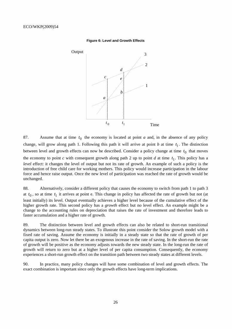
89. The distinction between level and growth effects can also be related to short-run transitional dynamics between long-run steady states. To illustrate this point consider the Solow growth model with a fixed rate of saving. Assume the economy is initially in a steady state so that the rate of growth of per capita output is zero. Now let there be an exogenous increase in the rate of saving. In the short-run the rate of growth will be positive as the economy adjusts towards the new steady state. In the long-run the rate of growth will return to zero but at a higher level of per capita consumption. Consequently, the economy experiences a short-run growth effect on the transition path between two steady states at different levels.

90. In practice, many policy changes will have some combination of level and growth effects. The exact combination is important since only the growth effects have long-term implications.

Time

Output

1

2

3

a

c

b

e

d

0 t 1t

ECO/WKP(2009)54

27

5.2 Tax Reforms

91. Appendix 2 demonstrates the surprising and strong result that the long-run optimal tax rate on capital should be zero. Although the derivation in the appendix is undertaken for an exogenous growth model, the result also applies when growth is endogenous. The basic intuition that the intertemporal allocation should not be distorted applies equally in both cases. This is an important conclusion since it contrasts markedly with observed tax structures. For example, in 2002 the top corporate tax rate was 40% in the US, 30% in the UNITED KINGDOM and 38.4% in Germany. Although Ireland was much lower at 16%, the OECD average was 31.4% (Hindriks and Myles, 2006).

92. In addition to the corporation tax most countries employ an income tax that taxes the return to saving. This lowers the net return earned on assets and results in a disincentive to save. This leads to a lower rate of capital accumulation. The divergence of the observed tax rate from the theoretically optimal rate and the taxation of saving raises the possibility that a reform of the actual system can raise the rate of economic growth and the level of welfare. This question has been tested by simulating the response of model economies to policy reforms involving changes in the tax rates upon capital and labour. Such studies have provided an interesting range of conclusions that are worth close scrutiny.

93. The basic model for simulation analysis is an endogenous growth model with both physical and human capital entering the production function. The consumption side is modelled by a single, infinitely lived representative consumer who has preferences represented by the utility function

[ ]∑−

=∞

=

−

0

1

1

1

ttt

t LCUσαβ

σ, (54)

where tC is consumption and tL is leisure. Alternative studies adopt different values for the parameters

α and σ . The second area of differentiation between studies is the range of inputs into the production process for human capital, in particular whether it requires only human capital and time or whether it also needs physical capital. The analytical process is to specify the initial tax rates, which usually take values close to the actual position in the US, and calculate the initial growth path. The tax rates are changed and the new steady state growth path calculated. The two steady states are then contrasted with a focus placed upon the change in growth rate and in levels of the variables.

94. Table 2 summarises some illustrative policy experiments and their consequences. The experiment of Lucas (1990) involves elimination of the capital tax with an increase in the labour tax to balance the government budget. This policy change has virtually no growth effect (it is negative but very small) but a significant level effect. In contrast, King and Rebelo (1990) and Jones et al. (1993) find very strong growth and level effects. King and Rebelo consider the effect of an increase in the capital tax by 10 percentage points whereas Jones et al. mirror Lucas by eliminating the capital tax. What distinguishes the King and Rebelo analysis is that they have physical capital entering into the production of human capital. Jones et al. employ a higher value for the elasticity of labour supply than other studies. The model of Pecorino (1993) has the feature that capital is a separate commodity to the consumption good. This permits different factor intensities in the production of human capital, physical capital and the consumption good. Complete elimination of the capital tax raises the growth rate, in contrast to the finding of Lucas.

95. The importance of each of the elements in explaining the divergence between the results is studied in Stokey and Rebelo (1995). Using a model that encompasses the previous three, they show that the elasticity of substitution in production matters little for the growth effect but does have implications for the level effect - with a high elasticity of substitution, a tax system that treats inputs asymmetrically will be more distortionary. The elimination of the distortion then leads to a significant welfare increase. The

ECO/WKP(2009)54

28

important features are the factor shares in production of human capital and physical capital, the intertemporal elasticity of substitution in utility and the elasticity of labour supply. Stokey and Rebelo conclude that the empirical evidence provides support for values of these parameters which justify Lucas' claim that the growth effect is small.

Table 2: Growth Effects of Tax Reform

96. These simulations models produce a variety of results but provide only limited insight into the general outcome. A number of analytical results are provided in Milesi-Ferretti and Roubini (1998). The model they consider encompasses most of those described above. It has separate production technologies for physical and human capital. Interestingly, it considers three different interpretations of leisure. In the first interpretation leisure is the usual residual time that is not spent working or studying to raise human capital. This is termed the “raw time” model. The second interpretation, “home production”, has leisure produced through a production function using human and physical capital. The third interpretation just uses time and human capital in the production of leisure. This is termed “quality time”.

97. The policy experiments consider the marginal increase of a particular tax with the government budget balanced by a change in the lump-sum transfer to the representative consumer. With this in mind it is not surprising that the results reported in Table 3 show that an increase in the tax rates generally reduce the steady-state rate of growth.

Capital 0% Labor 0% Growth 2.74%




Final Position Additional Observations

Initial Tax Rates and Growth Rate

Utility Parameters

FeaturesAuthor

Capital and consumption different goods, consumption tax replaces income taxes


σ = 2

α = 0.5

Production of human capital requires physical capital

Pecorino (1993)

10% increase in capital stock 29% increase in consumption


σ = 2

α= 4.99

α calibrated given σ

Time and physical capital produce human capital

Jones, Manuelli and Rossi (1993)

Labor supply is inelastic


σ = 2

α = 0

Production of human capital requires physical capital (proportion = 1/3)

King and Rebelo (1990)



σ = 2

α = 0.5

Production of human capital did not require physical capital

Lucas (1990)





Final Position Additional Observations

Initial Tax Rates and Growth Rate

Utility Parameters

FeaturesAuthor

Capital and consumption different goods, consumption tax replaces income taxes


σ = 2

α = 0.5

Production of human capital requires physical capital

Pecorino (1993)



σ = 2

α= 4.99

α calibrated given σ

Time and physical capital produce human capital

Jones, Manuelli and Rossi (1993)

Labor supply is inelastic


σ = 2

α = 0

Production of human capital requires physical capital (proportion = 1/3)

King and Rebelo (1990)



σ = 2

α = 0.5

Production of human capital did not require physical capital

Lucas (1990)

ECO/WKP(2009)54

29

Table 3: Effect on Steady-State Growth Rate

Model Capital income Labor income Consumption

Raw time Decrease Decrease Decrease

Home production Decrease Decrease No effect

Quality time Decrease

Source: Milesi-Ferretti and Roubini (1998)

98. An alternative perspective is provided by Song (2002) who employs a version of the Blanchard (1985) overlapping generations model with perpetual youth. (The perpetual youth label arises from the fact that each consumer has an equal probability of survival into the next period.) The analysis is based on the assumption that all government revenues are spent unproductively so there is no expenditure effect on growth. The argument of the paper builds on the observation that in this model the growth rate of consumption is increasing in the after-tax interest rate and in the share of human wealth in total wealth. A higher rate of tax that lowers the after-tax interest rate can still cause growth to rise if it raises the share of human wealth. The paper finds that a higher rate of tax on income (meaning both capital income and labour income) raises the steady state growth rate if and only if the elasticity of factor substitution is greater than 1. This is a strong restriction for the elasticity to satisfy. The result is also shown to extend in a weaker form to an economy where physical capital is used as an input into the learning process.

99. Although it does not directly address issues in endogenous growth the analysis of Hendricks (2003) merits reporting. An initial inspection of the Ramsey growth model and the overlapping generations model make them seem entirely distinct. The observation of Hendricks is that the only significant distinction is the degree of inter-cohort persistence. A pure overlapping generations model has no persistence: each consumer lives for two periods and there is no transmission of wealth between generations. The Ramsey model with a consumer whose life is infinite has complete persistence: decisions take into account the entire lifetime trajectory of welfare.

100. Hendricks explores the claim that persistence affects the tax elasticity in a model encompassing the Ramsey model and the overlapping generations model. The model has two key parameters. One parameter determines whether the bequest motive is operative. The other parameter determines whether there is any link between the human capital of parent and offspring. Varying the values of these parameters allows the transition between Ramsey model and overlapping generations model. Simulations are conducted for five variants of the model. Stronger persistence increases the steady-state tax elasticity of human capital for both wage and capital income taxes. Infinite lives models have higher elasticities than overlapping generations models. The message of the paper is that the specification of the model matters for the tax elasticity that is derived.

101. Keuschnigg and Deitz (2005) propose a change to the standard income tax system that they claim will promote growth. The proposed tax structure consists of four parts: i) a progressive tax of labour income; ii) a flat tax on company profits (both corporate and non-corporate); iii) deduction of interest payments and normal return to equity from taxable profit of firms; and iv) a proportional tax at the personal level on all forms of capital income. The rates are chosen to prevent arbitrage through shifting between labour income and profit income for owners of firms. The proposed structure has elements of a dual income tax system because of the different treatments of labour and capital income. The paper proves that this system is neutral with respect to the allocation of capital across sectors.

ECO/WKP(2009)54

30

102. The effect of the proposal is simulated by placing it within an overlapping generations model. The simulations show that long-run GDP will rise by between 2 or 3% if the system is implemented. Note that this is the level of GDP and not the rate of growth, so that it seems to be a large change in tax system for a small change in welfare. Since the model is one with overlapping generations there can be no long-run growth, so the analysis may not really be capturing the full growth effect of proposed tax system revisions.

103. This section has reported on the range of estimates that have been obtained for the effects of taxation upon growth. Some of the models predict that the growth effect is insignificant, others predict it could be very significant. What distinguishes the models are a number of key parameters, particularly the share of physical capital in human capital production, the elasticities in the utility function and the depreciation rates. In principal, these could be isolated empirically and a firm statement of the size of the growth effect given. To do so and thus claim an “answer” would be to overlook several important issues about the restrictiveness of the model. It would also overlook detailed information that is available upon how taxation affects each component of growth.

5.3 Components of Growth

104. The endogenous growth model with human capital accumulation is only one model from the many available. A review is now undertaken of a range of models that either model human capital accumulation in more detail or consider other sources of endogenous growth.

5.3.1 Education

105. An early model of the link between education and growth is described in Weale (1992). The paper discusses the channels through which education (and fertility) can affect growth and health, and the measurement of the social rate of return to education. It is observed that the high returns to education that have been calculated for developing economies may represent the consequence of short-term shortages of educated labour and the effect of omitted variables in regression equations.

106. A simple model is provided in which a dynasty chooses the investment in education for each generation and the number of offspring. The dynastic choice is then embedded in a growth model and a simulation analysis is conducted. The interesting finding of the paper is that the rate of growth is positively related to the chosen amount of education but negatively related to fertility. The major insight is viewed as the link between reduced fertility and increased education.

107. Trostel (1993) provides a model of investment in human capital that can be interpreted as representing educational choice. In this model human capital formation requires the investment of time and the investment of commodities. The commodities can either be bought indirectly through the firm of employment or directly on the market. The difference is that when purchased through the firm the goods are subsidised by the tax system (in the sense that they are tax deductible) but lead to a lower income since the firm deducts the cost from payment. Goods bought directly for human capital investment are subsidised by the government. The consumer optimises over all decision variables.

108. The model is simulated using a parameterisation justified by appeal to the econometric literature. What the basic simulation shows is that the effect of an increase in the proportional income tax is focused on the human capital level, rather than on the labour hours variable. This implies that 80% of the adjustment in the product of labour and human capital (LH - the effective labour input) is through human capital, H. The results are summarised in Table 4. All symbols have standard meaning except for x which is the proportion of total time spent in human capital formation. The column labelled long-run equilibrium reports the percentage change in the variable for a percentage change in the income tax rate. Hence, an

ECO/WKP(2009)54

31

increase in income tax from 40% to 40.4% reduces human capital by 0.388%. The second column is the present value of the time path of percentage changes per present value of percentage change in the tax rate. Hence, the discounted average decrease in human capital is 12%.

Table 4: Income Tax Elasticities

Variable Long run

equilibrium

Present

value

H -0.388 -0.123

y -1.146 -0.802

xH -0.480 -0.280

LH -0.480 -0.291

K -1.368 -0.597

w -0.222 -0.077

r 0.667 0.230

Source: Trostel (1993)

109. Particular parameterisations of the general model capture alternative models that have been used previously and these have different implications for the response to taxation. From the perspective that the general model is correct Trostel thus concludes that other models can be wrong. In summary, this analysis provides theoretical evidence that the effect of taxation on human capital accumulation can be large. The paper indicates that the change in investment in human capital can be more important than the change in working hours due to taxation. Hence, it is concluded that taxation significantly discourages human capital investment.

110. The ideas of Trostel are further developed in Heckman et al. (1998). This paper studies a version of the Auerbach-Kotlikoff (1987) model in which there is individual heterogeneity. There are several human capital (or skill) levels from which individuals make a selection. The heterogeneity is reflected in different individuals making different choices. The central focus of the analysis is the comparison of a progressive labour income tax with flat income and consumption taxes. Basic economic reasoning suggests that a move to a flat tax will encourage skill accumulation since it raises the incentive to seek higher income, and the consumption tax will encourage physical capital accumulation since it removes the tax on interest income. A selection of the results is presented in Table 5. The change in the stock of human capital for the two tax reforms confirms the intuition that a progressive labour income tax discourages education. In both cases the aggregate level of output increases.

ECO/WKP(2009)54

32

Table 5: Effect of tax reform on capital and output

Percentage change from

equilibrium with progressive tax

Flat tax Consumption tax

Stock of

physical capital

-0.79 4.65

Stock of college

human capital

2.82 1.85

Stock of high-school

human capital

0.90 0.08

Aggregate

output

1.15 4.98

Source: Heckman et al. (1998)

111. It is observed in Myles (2007a) that standard cross-country regressions reveal a positive relationship between the quantity of schooling in a country and the growth rate. Bils and Klenow (2000) explore the factors that can explain this observation. They build an endogenous growth model with a schooling choice. The model has the property that the causality between education and growth runs in both directions. Schooling develops human capital, and so raises the rate of growth. In the reverse direction, the effect of higher growth is an increase in the return to education, so the investment in education rises. A version of the model is calibrated using UNESCO data on educational attainment. The calibrated model is used to justify the claim that the impact of schooling on growth explains less than one third of observed cross-country correlation between education and growth. Instead, the growth to schooling effect is assessed as being potentially large.

112. Increased schooling can raise the level of human capital. If this schooling is publicly provided then revenue must be raised to finance the provision. The tax instrument chosen to raise the revenue can introduce distortions into the economy and has implications for the rate of growth. It is therefore not correct to infer that increased public education will necessarily raise growth without specifying the financing mechanism. These issues have been explored in a range of models.

113. Blankenau and Simpson (2004) observed that theoretical analysis predicts government expenditure on education increases the stock of human capital and should therefore raise the growth rate. However, this effect does not appear to be especially apparent in the data. The reconciliation between these two observations that is offered in the paper is that the taxes imposed to finance educational spending have distortionary effects. The distortions caused by the taxes then result in an offsetting reduction in the growth rate.

114. This idea is tested by constructing a model with overlapping generations and a range of tax variables (labour, capital, consumption, and output). When a nondistortionary output tax is used to finance expenditure there is a non-monotonic relation between spending and growth, so that growth first rises with spending and then falls. With a consumption tax used instead of the output tax the level of growth always

ECO/WKP(2009)54

33

rises with expenditure. The effects of labour and capital taxes are less clear, but cases are found where the relationship between spending and growth is non-monotonic.

115. The finding of non-monotonicity can be used to help understand the empirical results. The countries observed in a data set may be either side of the divide between growth increasing with spending and growth decreasing with spending. If this is the case it follows that when a regression analysis is undertaken there will be no clear relationship between education expenditure and growth. A similar argument is discussed in Myles (2007a) in connection with the work of Slemrod (1995). The results also confirm that the tax policy used to finance expenditure has important consequences for growth.

116. It is not necessary that education is provided publicly. Since there is a private benefit to human capital accumulation some investment in education (but not necessarily the efficient level if there are externalities or other imperfections) will be made and financed privately even if there is no public provision. A government therefore has the choice of either relying on private choices, providing education publicly, or subsidising private investment.

117. Ciriani (2007) addresses these different methods of educational financing. The setting is an extension of the model of Zhang (2005) that incorporates random ability shocks on human capital. The random shocks result in workers having different inherited abilities to learn. The human capital of each worker is determined as the product of inherited ability, spending by parent, and average spending in society. Parents are altruistic and care about the human capital of their offspring. This provides an intertemporal linkage.

118. The paper contrasts three financing systems: i) private provision; ii) free uniform public provision financed by an income tax; and iii) subsidisation of private provision financed by an income tax. The results show that subsidisation can lead to higher growth than either of the other two in the short run. Subsidisation can also lead to higher growth in the long run if the dispersion of inherited ability to learn is sufficiently low. In terms of the points made by Blankenau and Simpson (2004) it is important to observe that Ciriani (2007) determines the spending and tax policies simultaneously, so these result describe the net effects on growth of the government policy.

119. In the model of Ciriani (2007) all uncertainty is resolved before the human capital choice is made. Krebs (2003) makes the alternative assumption that there is still risk at the time at which the investment decision is taken. This causes there to be a link between the tax system, its interaction with risk, and the choices made.

120. Krebs (2003) analyzes a model in which households face a choice between investment in physical capital and investment in human capital. The return from physical capital is risk free. In contrast, the return from human capital investment is risky in that there is an idiosyncratic shock each period which can add to, or reduce, the stock of human capital. As a consequence of risk aversion the choice of investment is biased toward physical capital because of the risk to the return on human capital. This implies that if a reduction can be secured in the risk on human capital then the level of physical capital investment will be reduced and the level of human capital investment will be raised. A policy aimed at reducing risk can therefore benefit growth since it leads to a more balanced allocation of investment. The analysis shows that this reallocation of investment effect can be so significant that even when a distortionary income tax is used to provide insurance against human capital risks both growth and welfare can increase. The importance of this paper is that it provides a new perspective from which to think about the role of an income tax in affecting growth.

121. The decision to invest in human capital is affected by the discounted lifetime flow of income. In most analysis only the income from employment is considered in the lifetime flow but, although it is

ECO/WKP(2009)54

34

highly discounted at the time most human capital investments are made, the income from social security in retirement is also a factor. Lau and Poutvaara (2006) observe that the social security system affects the private return to an investment decision if the expected flow of social security is dependent upon the flow of income when working. There will also be a link between social security and the equilibrium return through the consequences of individual decisions for the aggregate capital stock. The major finding of the paper is that linkage between social security benefits and contributions made while working raises the level of human capital investment.

122. The role of public subsidisation of education is further developed in Benabou (2002). A model is constructed in which consumers produce using their own labour and accumulated human capital. The equilibrium effect of a progressive income tax and a progressive redistribution to educational expenses are determined. It is shown that the intertemporal distortion caused by the income tax can be offset by other policies which are unanimously supported by the population of consumers. The numerical works trades off efficiency and equity to characterise an optimal interior policy. The unusual feature of the model is that there is no interaction between consumers in the market place. Each agent produces and consumes their own output less what the government subtracts or adds in redistribution. Hence, this is a model of economic activity that has no trade.

123. In the context of growth theory the use of college scholarship programmes can be seen as a method of increasing the accumulation of human capital. The success of the programmes in raising human capital is primarily dependent on the responsiveness of the demand for education. Evaluation of the responsiveness is an empirical issue which is discussed in Myles (2007b). The issue that is now analyzed is how the means-tested nature of scholarship programmes interacts with other economic choices and policies. The point is that the scholarship programmes cannot be treated in isolation but must be viewed as part of the overall household decision process.

124. The analysis of Feldstein (1995a) demonstrates that the structure of college scholarship programme can have a negative effect on saving. In this case a programme that is designed to provide means-tested assistance to encourage human capital accumulation can damage growth by acting adversely on one of the other sources of growth.

125. The argument is that college scholarships are assessed on the basis of parents' ability to pay. This takes into account income and assets. The scholarship is reduced as asset holdings increase, so this provides a disincentive to save. Feldstein assumes that the system can be given the simple representation

( ) βθα +−= AES for ES ≤≤0 , (55)

where S is the scholarship received, E is the cost of college, A is the asset holding of the parents, α is the rate of adjustment of the scholarship, β is any lump-sum grant received, and θ is the marginal rate of tax on accumulated assets used to calculate the parental contribution. The saving effect comes from the fact that as A rises the value of S falls. This is equivalent to a higher rate of taxation applied to asset holding. An analysis of the lifecycle decision of the parents shows that an increase in θ reduces the optimal A and E. The effect upon E can be interpreted as the choice of a cheaper college. The effect of an increase in α on choices is ambiguous, but it may also reduce A.

126. The empirical analysis uses data from the 1986 Federal Reserve Board Survey of Consumer Finances and restricts attention to a homogenous group of households (married couple, head between 40 and 50, children under 18 but none in college, annual income positive but not more than $100,000). Let the annual capital levy on assets under the scholarship programme be t. This value is increasing in the level of income. A family with children who will, in total, spend n years in education face an education capital tax

ECO/WKP(2009)54

35

of ( )nt−−= 11θ . Because of the behavior of t the education capital tax also increases with income until a maximum is reached, then remains constant until the maximum qualifying income level is reached. Instrumental variable estimation generates the regression equation (with standard errors in parentheses)

( ) ( ) ( )

YAGEA

+−−+−=

026.060.014.1076.041.104.2934,9 θ , (56)

where AGE is the age of the household head and Y is household income.

127. The estimated equation shows that the educational tax has a negative and significant effect upon asset accumulation. A family with income of $40,000 and a head aged 45 with two children differing in age by 2 years would face the maximum annual capital levy of 0846.0=t . The assumptions imply

6=n and 41.0=θ . The regression predicts that this family would have reduced asset accumulation by $23,124.

128. The paper concludes that educational scholarship programmes can have a major impact upon the level of saving. The structure of the programmes provide a disincentive to save. When aggregated over households in the economy the result implies a significant reduction in saving for the economy. There is therefore a conflict between saving and encouraging human capital formation through scholarship programmes.

129. A separate form of interaction is analyzed by Dynarski (2004). An incentive to save for education is provided by 529 Savings Plans and Coverdell Savings Accounts. The basis of these schemes is that the returns to saving are tax free if the withdrawals are used to finance education. The point of the paper is to analyze the interaction of these incentives with the aid packages granted by colleges. The important conclusion is that the interaction means that the marginal tax rate is in excess of 100% for some middle income families. This results from aid being withdrawn because of the higher return on the savings plans. The implicit message is that this is should be avoided but the paper does not explicitly address the effect on educational investment.

130. The accumulation of human capital does not have a single homogenous form. There are different levels of education (primary, secondary, etc.) and different forms of training (specific and general). Analyzing the aggregate level of human capital in an economy can overlook some of the finer detail that can influence the rate of economic growth. Most empirical analysis considers only the division into different levels. Some recent work theoretical work has tried to move beyond this to explore the implications of different forms of human capital accumulation.

131. Krueger and Kumar (2004) note that there has been a widening of the growth differential between the US and Europe. During the 1970s there was little difference in growth rates between the two regions. But through the 1980s, and especially in the 1990s, the US grew consistently faster than Europe. The paper observes that this has occurred during the new “information age” and that the US has been noticeably faster in the adoption of new technology. An explanation is provided as to why this might be so.

132. The answer proposed is that human capital can take either a general form or a specific form. Two claims then support the analysis. First, that the specific form of human capital is the outcome of vocational training. Second, that the general form of human capital allows much quicker adaptation to new technology. Evidence is presented to show that Europe has concentrated more on vocational training and the US has concentrated more on general training. The basic component of this evidence is presented in Table 6. This shows the division of the secondary education population between general and vocational training. In the US there is no separate vocational stream. The table also reports the entry rate into

ECO/WKP(2009)54

36

university. The paper asserts that university provides general training so arrives at the conclusion that the US has much less vocational training than Europe.

Table 6: Education indicators

% upper

sec. in

general

% upper

sec. in

vocational

University

net entry

rate

Austria 23 77 26

Finland 48 52

France 47 53 33

Germany 23 77 27

Italy 28 72

Netherlands 30 70 34

Sweden 44 53

EU 42.4 57.6

United States 52

Source: Krueger and Kumar (2004)

133. A model is constructed that captures these two features. Households choose between specific and general training. General training is costly to obtain. Firms select the rate of adoption of new technologies. It is shown that the model can replicate some of the claims: an economy with relatively more vocational training will not grow as fast as one with general training when there is technological advance. This conclusion is interesting but not absolutely compelling. The US has seen redundancies and has experienced significant costs of adjustment in the move from traditional manufacturing industries to new information technology industries. There is also the fact that the US has probably relied on a considerable quantity of imported labour in the high technology sectors. This is not reflected in the education data presented by the paper. The division of human capital into the two forms also seems unconvincing when one tries to categorise various educational programmes into vocational or general.

134. The analysis of Blankenau (2005) considers how the division of expenditure between lower-level education and higher-level education may affect growth. The model employed has an overlapping generations structure. It is assumed that low-level education is compulsory but high-level education is optional. Part of the cost of high-level education may be funded by the government, but the remainder has to be financed privately. The return to high-level education is an increase in income. The paper focuses on the best allocation of government expenditure to the two levels of education. The tax instrument used to finance government expenditure is a lump-sum tax on income and so is non-distortionary. It is demonstrated that high-level education should only be subsidised once a critical level of expenditure is reached. Prior to this level being reached all expenditure should be on low-level education. This is not

ECO/WKP(2009)54

37

surprising when there are decreasing returns to low-level education, the return to high-level education can be privately captured in higher wages, and there is a perfect capital market so nothing restricts efficient individual investment in high-level education.

5.3.2 Research and Development

135. The model of endogenous growth through innovation makes clear the importance of research and development (R&D). Aghion and Howitt (1992) emphasise the fact that a competitive market may not generate an efficient outcome because of the externalities associated with R&D. It is these externalities that have motivated research that estimates the private and social returns to innovation. If these returns are not aligned then there is potential for economic policy to enhance efficiency by countering the effect of the externality.

136. Jones and Williams (1998) build on the modelling of innovation in endogenous growth models to calculate the social rate of return to R&D and, hence, to contrast the optimal amount of R&D with the equilibrium amount. The idea used is to take a production function for output and a production function for “ideas” and to use these to consider the following variation from the equilibrium path: reduce consumption today, raise R&D today, reduce R&D tomorrow (to keep future path of ideas the same) and ask how much output goes up. No private individual will wish to undertake this variation (since it is assumed that each is optimising). But if there are any externalities or distortions society may wish to make the deviation. The social return to R&D is the gain in consumption from this variation. The central feature of the analysis is that the construction of the social return does not depend on market conditions but only upon production possibilities. What the market determines is where on the trade-off between R&D and consumption the economy is located.

137. The paper proceeds to set out a growth accounting methodology for evaluating the component of total factor productivity generated by R&D. This leads to the change in TFP being regressed on the share of R&D expenditure in GDP. The estimated coefficient gives the return. Table 7 summarises results that studies using this methodology have obtained. The variable r (own) is the return on privately financed R&D. The variable r (used) is the return on R&D in one industry financed by R&D expenditure of another industry. The value of Sum is the social return to R&D. The studies report high estimates of both the private and social return: own R&D has a return on 27% and the spillover has a return of about 70%, so the social return is 100%.

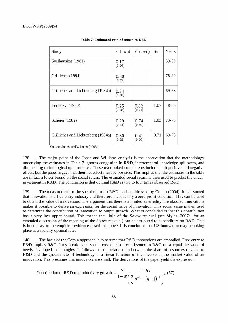
ECO/WKP(2009)54

38

Table 7: Estimated rate of return to R&D

Study r (own) r (used) Sum Years

Sveikauskas (1981) ( )06.0

17.0 59-69

Grilliches (1994) ( )07.0

30.0 78-89

Grilliches and Lichtenberg (1984a) ( )08.0

34.0 69-73

Terleckyi (1980) ( )08.0

25.0 ( )21.0

82.0 1.07 48-66

Scherer (1982) ( )14.0

29.0 ( )39.0

74.0 1.03 73-78

Grilliches and Lichtenberg (1984a) ( )09.0

30.0 ( )20.0

41.0 0.71 69-78

Source: Jones and Williams (1998)

138. The major point of the Jones and Williams analysis is the observation that the methodology underlying the estimates in Table 7 ignores congestion in R&D, intertemporal knowledge spillovers, and diminishing technological opportunities. These overlooked components include both positive and negative effects but the paper argues that their net effect must be positive. This implies that the estimates in the table are in fact a lower bound on the social return. The estimated social return is then used to predict the under-investment in R&D. The conclusion is that optimal R&D is two to four times observed R&D.

139. The measurement of the social return to R&D is also addressed by Comin (2004). It is assumed that innovation is a free-entry industry and therefore must satisfy a zero-profit condition. This can be used to obtain the value of innovations. The argument that there is a limited externality in embodied innovations makes it possible to derive an expression for the social value of innovation. This social value is then used to determine the contribution of innovation to output growth. What is concluded is that this contribution has a very low upper bound. This means that little of the Solow residual (see Myles, 2007a, for an extended discussion of the meaning of the Solow residual) can be attributed to expenditure on R&D. This is in contrast to the empirical evidence described above. It is concluded that US innovation may be taking place at a socially-optimal rate.

140. The basis of the Comin approach is to assume that R&D innovations are embodied. Free-entry to R&D implies R&D firms break even, so the cost of resources devoted to R&D must equal the value of newly-developed technologies. It follows that the relationship between the share of resources devoted to R&D and the growth rate of technology is a linear function of the inverse of the market value of an innovation. This presumes that innovators are small. The derivations of the paper yield the expression

Contribution of R&D to productivity growth

( )

−−

−−

=−− 11 1

1 ηηααα

s

gr Y , (57)

ECO/WKP(2009)54

39

where α−1 = labour share in output, YRs /= , R = spending on R&D, Yg is the growth rate of output, η is the inverse of the elasticity of substitution between different intermediate goods in production. The

expression in (57) is plotted in Figure 7 using the parameters r = 0.07, Yg = 0.034, α = 0.33, r = 0.07. The upper line in the figure is for η = 1.2, and the lower line for η = 1.5. Note that for both values the graph has a discontinuity for slightly larger values of s. At the R&D intensity observed in the US (s = 0.2) the R&D contribution represents only one tenth of the annual growth rate of 2.2%. To account for all the productivity growth in the US the R&D intensity must be s = 4.8 when η = 1.5, and η = 8 when η = 1.2. These observations led the paper to conclude that much of the growth in TFP is unexplained.

Figure 7: Contribution of R&D to productivity growth

141. An important feature of R&D is that the spillover effects are not contained within national borders. For example, innovation in computing hardware in the US rapidly diffuses across the world. This raises the level of technology in every country that adopts the new hardware. The adoption of technology created elsewhere is likely to be the major source of growth for many countries. Such observations have motivated extension of the innovation model to an international setting.

142. Howitt (2000) develops the model of Schumperterian innovation by creative destruction to fit within an international setting. The basic structure of the model is that firms invest in R&D and innovations arrive randomly, but at a rate influenced by the R&D expenditure. The innovations transfer across countries. The transmission mechanism is that if a country makes the next innovation the level of innovation will be above the maximum achieved anywhere in the world. Hence, an innovation leapfrogs a country to the top of the technology ladder. Implicitly, this is assuming that all countries have access to the best available technology (or at least knowledge of that technology) and can improve upon it by innovation. Other than this self-produced innovation there is no other transmission mechanism for technology to diffuse. It might be expected that technology would filter down through trade or through foreign direct investment but these processes are not incorporated within the model.

143. As a consequence of the assumptions a country that does not spend on R&D simply stagnates. It is claimed that this model generates relationships between growth and economic variables that are essentially the same as for the Solow model but with the inclusion of some additional terms. Hence, the regressions that fit reasonably well with the Solow model do not show that endogenous growth models are inappropriate but in fact may be miss-specified. It is argued that the miss-specification results in an over estimate of the capital share in generating growth. These comments relate to the controversy begun by Mankiw et al. (1992) and discussed further in Myles (2007a). The representation of growth is interesting

ECO/WKP(2009)54

40

for the debate on endogeneity, but the international transmission mechanism for innovation is limited in scope.

144. Diao et al. (1999) present an alternative endogenous growth model that accounts for international spillovers of technology. The model is based on each country possessing an aggregate production function for R&D. Incorporated within this production function are two spillover effects. First, the output of R&D is proportional to the total level of accumulated knowledge with each country. Second, there is an international spillover. The international spillover arises from the trade in investment goods. The purchase of investment goods from abroad is viewed as adding to the total stock of knowledge through the technology embodied in those goods. The model is calibrated to data for Japan and employed to study the effects of trade policy and policies designed to stimulate R&D. It is shown that strategic trade policy does not increase R&D at home significantly, but can increase the spillover effect which in turn raises growth. Conversely, trade liberalisation can reduce growth. Policies that directly subsidise R&D are found to have significant growth-enhancing effects at a low net cost to taxpayers.

145. The potential inefficiency of the competitive equilibrium when there is innovation provides scope for efficiency-enhancing policy intervention. This has led to studies of the effect of tax policies on R&D.

146. Lin and Russo (2002) compare the consequences of cuts in capital taxation in a model with exogenous innovation to the effect in a model with endogenous innovation. When innovation is exogenous a cut in the capital tax raises the level of saving. When innovation is endogenous a cut in the tax raises innovation as well. The model is then calibrated to fit US data. This exercise suggests that the exogenous innovation model underestimates the effect of tax cuts on innovation.

147. It is often observed that the private R&D choices of a firm do not take into account the losses imposed on previous innovators nor on possible duplication, so there is potential that R&D may undertaken at too high a level. However, private choices also do not take into account the social return, so providing a reason for R&D expenditure to be too low. Russo (2004) notes briefly some limitations of the empirical work on R&D as a justification for conducting a CGE study to rank the effectiveness of different tax schemes. The model used is based on those of Romer (1990a) and Jones (1995). Labour effort is an input into the advancement of knowledge. There are potential spillover effects, potential duplication effects, and crowding effects. The simulation results that are given emphasis are that: i) incremental and comprehensive R&D tax credits produce relatively large increases in research effort and welfare; ii) lower income tax rates and tax credits for downstream users rank next; iii) investment tax credits for upstream producers are ineffective; and v) incremental credits dominate comprehensive credits.

5.3.3 Government spending

148. Government expenditure can be used for consumption or for the provision of a public capital good. The model of Barro shows how growth can be sustained by accumulation of the public capital good. The inclusion of this effect in a simulated policy experiment changes the manner in which taxation affects growth.

149. Baier and Glomm (2001) extend the simulations of Section 4.3. The basic assumption is that the set of productive inputs is expanded to include physical capital, human capital and a publicly-provided input. This provides a positive role for taxation to finance the public expenditure. Government expenditure is divided between investment in the productive input, provision of a utility-enhancing service, and transfer payments. These expenditures are financed by distortionary taxes on capital and labour.

150. The paper provides some analytical results for the special case of a Cobb-Douglas production function and some simulations. The main results are that the growth rate increases the higher is the

ECO/WKP(2009)54

41

proportion of government revenue spent on the productive input relative to the proportion that is redistributed, and that the optimal tax on capital is positive. The positive tax on physical capital is interpreted as recovering some of the return to public capital (or, alternatively, putting a price on public capital for the private firm). Simulations of a CES technology support the result that the growth rate is increasing in the proportion of government expenditure on investment. Holding spending patterns fixed and increasing the tax rate ultimately decreases the growth rate (although it may increase for low tax rates). The paper captures some aspects of the simultaneity between taxation and public expenditure that is apparent throughout the empirical literature.

151. Many of the policy experiments consider only tax systems with a constant marginal rate. This is typically for reasons of analytical and computational simplicity. An exception to this is the work of Li and Sarte (2003) who analyze the consequences of progressive taxation. The basic assumption is to capture progressivity by a single parameter. To achieve this a progressive tax function is defined by

φ

ζτ

=

Y

y

Y

y, (58)

where φ measures the degree of progressivity. This tax function is embedded in two alternative endogenous growth models: Rebelo's model where government spending is not productive and Barro's model where government spending is an input.

152. The analysis focuses on how changes in taxes affect growth and income distribution and hence revenues via the progressive tax. The central observation is that the marginal rate of tax is endogenous and that more progressive statutory rates do not always imply more progressive effective rate - this can be caused by changes in the income distribution. The simulation analysis reports that the growth effect of a decrease in the marginal rate of tax relative to average rate of tax was positive but small. The size of the effects is summarised in the observation that the changes in US tax laws between 1981 and 1986 contributed at most 0.29% to per capita GDP growth.

153. The effect of switching from a progressive tax system to a flat rate tax system is simulated in Cassou and Lansing (2004). The focus of their analysis is the Hall-Rabushka flat tax proposal to place a single tax rate on all labour income above a threshold and on all capital income after fully expensing investment expenditures. The model has a single representative consumer who chooses physical capital and human capital use to maximise utility. Both forms of capital require investment of resource to be produced.

154. The simulations consider the consequences of reform from the current US tax system. The first step is to approximate the US system by the average tax rate (ATR) function

( )nATR ratio Income2528.0= , (59)

where n = 0.2144 and the income ratio is defined as income divided by mean income. Other parameters introduced are η which is the degree to which business income is double taxed, and kφ the fraction of

investment in physical capital that can be expensed. The outcomes of the policy experiments are shown in Table 8 where yg is the growth rate of output, τ is the mean personal tax rate, and bτ is the mean

business tax rate. All of the reforms raise the rate of growth with the single exception of maintaining progressivity in the tax structure. The greatest increase in growth occurs when the flat tax is introduced but η remains at the value of 1 (complete double taxation of business income). These results are further evidence that progressivity is harmful to growth in these simulation models.

ECO/WKP(2009)54

42

Table 8: Flat-tax reforms

Tax system Tax rate yg

Progressive tax system (US) 35.0,253.0 == bp ττ 1.800

Baseline flat tax reform 3437.0=τ 1.857

Reform with no change in kφ 3174.0=τ 1.854

Reform with no change in η 3169.0=τ 1.953

Reform with no change in n 3431.0=τ 1.638

Pure consumption tax reform 3520.0=τ 1.878

155. Some further implications of the division of government expenditure between consumption and investment are investigated by Chen (2006). The paper considers an endogenous growth model with a representative consumer. The government can divide its revenue between spending on consumption and spending on a productive input. The paper conducts an optimisation exercise and considers the effects of changes in parameters upon the optimal outcome. This exercise is intended to be related to the distinctions between countries and growth rates. The essence of the results is that changes in parameters have a direct effect upon growth and an indirect effect via the re-optimisation of the division between consumption and production. This leads to policy changes having stronger growth effects than predicted by models in which the government does not optimise.

5.3.4 Additional issues

156. There are further features of the growth process that have been investigated. The following papers consider international capital flows, inequality, and fertility.

157. Palomba (2004) constructs a two-country model. This has overlapping generations of consumers but an AK production structure to ensure endogenous growth. The key feature of the model is that capital is internationally mobile between the two countries and locates in whichever country offers the highest net return. Each country levies a source tax on capital invested in that country plus a tax on residents capital incomes regardless of source. These taxes determine the international allocation of capital via the equalisation of net rates of return. A variation in tax policy affects both the allocation of capital between countries and the total world stock of capital through the saving decisions of the consumers. The paper claims that a reduction in tax rates can increase the immediate amount of capital by obtaining a greater share of the existing stock, but ultimately lead to a fall in the growth rate. Therefore, what appears to be an attractive policy in the short run does not prove to be so in the long-run.

158. Benabou (1996) provides a detailed survey of the literature relating inequality to growth. Three mechanisms are identified that can generate a causal link between these two variables. First, distributional effects have an effect through the balance of power in the political system. The lower is the income of the median voter the more political support there is for redistribution. Redistributive expenditures can lessen

ECO/WKP(2009)54

43

incentives for risk-taking and innovation and reduce growth. Second, imperfections in credit markets prevent the poor from being able to undertake an efficient amount of investment. Because of this, their marginal product is higher than the equilibrium level, which can be exploited by redistribution to aid growth. An increase in redistribution reduces the capital market constraints faced by the poor and allows their investments to move closer to the efficient level. Third, sociopolitical conflict can reduce the security of property rights, which discourages accumulation. A widening income gap gives the poor an incentive to engage in rent seeking. Redistribution addresses both of these issues. For these reasons it is to be expected that there will be a negative correlation between growth and inequality in cross-country data.

159. The links between fertility and development are studied in Lord and Rangazas (2006). The paper claims that data support the argument that an increase in the schooling of younger children raises fertility as they become more valuable and can add to family income. In contrast, an increase in the schooling of older children reduces fertility because it raises the productivity of parents and the extra child income is not needed. The model is applied to long-run data from the US and England. It is also claimed that the move away from household production is also relevant for the changes in fertility. The model used is an overlapping generations one, so the growth component is limited.

5.4 Summary

160. This chapter has reviewed the contributions of a wide range of theoretical models. Simulation of the basic endogenous growth model with human capital accumulation produced a widely varying set of predictions. Amongst these predictions there is one element of constancy: none of the models contradicted the claim that a consumption tax will increase growth. It was also supported when more detailed modelling of the human capital decision was introduced. This is a result that will recur frequently in the review of empirical research.

161. The results also demonstrated that there can be two-way causality between the choice and growth. In particular, an increase in human capital accumulation raises growth and increased growth provides a greater incentive for human capital accumulation. This two-way causality is important when the results of growth regressions are discussed. Educational scholarship programmes are an example of a policy that at first sight appear only to be advantageous for growth. Closer inspection reveals that the means-tested structure of the programmes gives a disincentive to save because of the rate of withdrawal with respect to asset accumulation. Human capital rises, but the net effect on growth is uncertain if saving falls.

162. Finally, there are good arguments that the social benefits of R&D exceed the private benefits. This provides an argument for subsidising R&D with the intention of raising growth. The theoretical results also indicate that R&D may be sensitive to taxation. This later claim needs to be confronted with empirical evidence.

6. Conclusions

163. The purpose of this paper was to provide an introduction to the theory of economic growth and to review the simulation evidence on the effect of tax policy. The development of endogenous growth theory has provided many new insights the sources of economic growth. The essence of the new theory is that growth is a consequence of rational economic decisions. Firms expend resources on research and development to secure profitable innovations. Consumers invest in education to develop human capital and increase lifetime earning. Governments increase growth by providing public inputs, encouraging foreign direct investment, and enhancing educational opportunities. Through the aggregation of these individual decisions the rate of growth becomes a variable of choice, and hence a variable that can be affected by the tax policies of governments.

ECO/WKP(2009)54

44

164. The Solow growth model predicts consumption per capita will reach a limit unless there is technical progress. The source of technical progress is not modelled so the effect of policy cannot be analyzed. The model predicts economic convergence: countries with a low capital stock will grow faster than countries with a high capital stock. The most important conclusion concerning tax policy is that in the long-run it is inefficient to have a tax on capital income. Endogenous growth models provide an explanation of sustained growth. Several mechanisms through which growth can be sustained have been identified. The accumulation of human capital raises the supply of effective labour and demonstrates a theoretical role for education to raise growth. The existence of a productive public sector input can result in taxation having a beneficial impact on growth. The pursuit of innovation emphasises the value of Research and Development. Taxation can affect a range of personal and corporate choices that impact on growth.

165. Simulations of human capital models generate widely-varying outcomes for tax-reform experiments. Almost all the results support the claim that a move from income taxation to consumption taxation will raise the rate of growth even though the predicted effect may vary. The growth-increasing effect of moving from an income tax to a consumption tax is magnified when human capital accumulation is modelled. Scholarship programmes that assist with the financing of education can reduce the incentive to save through their interaction with the tax system. Research and development may have a high social value considerably in excess of its private value and expenditure on research and development may be sensitive to taxation.

166. Viewed from an endogenous growth perspective the link between taxation and growth seems self-evident. Corporate taxation affects the return to innovation and hence must affect the optimal amount of research and development. Personal income taxation reduces the returns to education so must reduce the accumulation of human capital. In simulations of economic growth models the effect of taxation on growth has frequently been demonstrated to be considerable. A clear presumption exists that data on economic activity must reveal a strong correlation between taxation and growth. The empirical evidence is reviewed in Myles (2007a, b).

ECO/WKP(2009)54

45

APPENDIX 1. CALCULATING GROWTH RATES

167. A number of results concerning the definition of growth rates and the manipulation of growth rates are used in this paper and the two companion papers. This appendix provides a self-contained summary of these results.

168. The growth rate of GDP can be measured in either discrete time or in continuous time. In discrete time the level of output at time t is denoted tY . In continuous time the level of output at t is ( )tY .

169. In discrete time the change in output between times t and 1+t is tt YYY −=∆ +1 . This can be

used to define the proportional rate of growth of output as

tt

tY Y

Y

Y

YYg

∆=−

≡ +1 . (A1)

In continuous time the rate of change is

dt

dYY ≡& , (A2)

so the proportional rate of growth is

Y

Y

Y

dtdYgY

&=≡ /

. (A3)

Observe that by the chain rule of differentiation

( )

Ygdt

dY

Ydt

Yd == 1ln. (A4)

This result is useful for two reasons. First, it allows development of expressions for per capita growth levels. GDP per capita is given by Y/L, where L is population size, so

( )dt

LYdg LY

/ln/ =

( ) ( )( )

dt

LYd lnln −=

ECO/WKP(2009)54

46

dt

dL

Ldt

dY

Y

11 −=

LY gg −= . (A5)

Hence the growth rate of GDP per capita is equal to the growth rate of GDP less the growth rate of population. Second, it allows decomposition of aggregate growth into a set of contributory factors. Let the aggregate production function have the Cobb-Douglas form

( ) ( ) ( ) ( ) αα −= 1tLtKtAtY . (A6)

Taking the log of both sides or (A6) gives

( )( ) ( )( ) ( )( ) ( ) ( )( )tLtKtAtY ln1lnlnln αα −++= . (A7)

Differentiating both sides of (A7) with respect to t and using (A4) gives

( ) LKAY gggg αα −++= 1 . (A8)

The factors K and L contribute to growth according to their shares in the Cobb-Douglas production function.

170. The division of aggregate growth into the contributions from different factors generalises to any production function of the form

( )LKAFY ,,= . (A9)

Differentiating both sides of A(9) with respect to t and dividing by Y gives

dt

dL

LL

F

Y

L

dt

dK

KK

F

Y

K

dt

dA

AA

F

Y

A

dt

dY

Y

1111

∂∂+

∂∂+

∂∂= , (A10)

or

LLKKAAY gggg ααα ++= , (A11)

where

z

F

Y

zz ∂

∂=α . (A12)

The analogue of the continuous growth rate can be calculated from data by using

( ) ( )( )0lnln1

YYt

g tY −= , (A13)

where 0Y is a base year and t is the time from 0 to t. Finally, the annual percentage growth rate (AGR)

averaged over a period of t years is defined by

ECO/WKP(2009)54

47

( ) ( )( ) 1001lnln1

exp 0 ×

−

−= YY

tAGR t . (A14)

This is the growth rate used in many of the growth regressions reported in Myles (2007a).

ECO/WKP(2009)54

48

APPENDIX 2. OPTIMAL TAXATION

171. The analysis of the fixed saving model has touched upon some of the potential consequences of policy intervention. As a tool for policy analysis, the model is very limited given the lack of choice variables that can be affected by policy. This shortcoming is now overcome by studying a variant of the Ramsey growth model in which a representative consumer chooses an intertemporal consumption plan to maximise lifetime utility. Using this model the optimal taxes upon labour and capital income can be derived. The derivation of the optimal tax rates given here is based on Hindriks and Myles (2006).

172. The Ramsey model has a single representative consumer who chooses the paths of consumption, labour and capital over time. The single consumer assumption is adopted to eliminate issues concerning distribution between consumers of differing abilities and tastes, and to place the focus entirely upon efficiency. For simplicity, it is also assumed that the growth rate of labour, n, is zero. There is a representative firm that chooses its use of capital and labour to maximise profits. Given that the market must be in equilibrium, the choices of the consumer drive the rest of the economy through the level of saving, and hence capital, that they imply. The supply of labour and capital from the consumer combine with the factor demands of the firm to determine the equilibrium factor rewards. The aim is to characterise the optimal tax structure in this economy.

173. It is assumed that the government requires revenue of amount tg at time t. It raises this revenue

through taxes on capital and labour, which are denoted by Ktτ and L

tτ respectively. The government

chooses these tax rates in the most efficient manner.

The choices of the consumer are made to maximise the discounted sum of the flow of utility. Letting 0 < β < 1 be the discount factor on future utility, the consumer's preferences are described by

( )∑=∞

=0,

ttt

t LCUU β . (A15)

The specification of the utility function implies that the consumer has an infinite life. This can be justified by treating the consumer as a dynasty with concern for descendents.

As there is a single consumer, the capital stock is equal to the saving of this consumer. This observation allows the budget constraint for the consumer to be written as

( ) ( )( ) ttKttt

Lttt KrLwKC τδτ −+−+−=+ + 1111 . (A16)

The utility maximisation decision for the consumer involves choosing the time paths of consumption, labour supply, and capital for the entire lifespan of the economy. The formal decision problem is

ECO/WKP(2009)54

49

{ }( ) ( )([∑ −+

∞

=0,,1,max

ttt

Ltt

ttt

t

KLCLwLCU

ttt

τλββ ( )( ) )]111 +−−−+−+ ttttKt KCKrτδ , (A17)

where tλ is the multiplier on the budget constraint at time t.

174. In solving this optimisation, it is assumed that the representative consumer takes the factor rewards tw and tr as given. This captures the representative consumer as a competitive price-taker. (It is

helpful to note that when the government optimisation is considered below the dependence of the factor rewards on the choice of capital and labour is taken into account by the government. This is what distinguishes the consumer who reacts to the factor rewards, and the government which manipulates the factor rewards.)

With fixed factor rewards, the necessary conditions for the choice of tC , tL and 1+tK are

0=− tCtU λ , (A18)

( ) 01 =−+ tLttL wU

tτλ , (A19)

and

( )( ) 011 111 =−−+− +++ ttKtt r λτδβλ . (A20)

Using the first condition to substitute for tλ in the second condition gives

( ) 01 =−+ tLtCL wUU

ttτ . (A21)

Stepping the first condition one period ahead and then substituting for 1+tλ in the third gives

( )( ) 011 111=−−+− +++ tt Ct

KtC UrU τδβ . (A22)

175. Conditions (A.21) and (A.22) describe utility maximisation by the consumer. To interpret these it should be observed that there are two aspects to the consumer's decision. Firstly, within each period the consumer needs to optimise over the levels of consumption and labour supply. The efficient solution to this within-period decision is described by (A.21) which ensures that the marginal utilities are proportional to the relative prices. Secondly, the consumer has to allocate their resources efficiently across time. Condition (A.22) describes efficiency in this process by linking the marginal utility of consumption in two adjacent periods to the rate at which consumption can be transferred through time via investments in capital. Taken together for every time period t, these necessary conditions describe the optimal paths of consumption, labour supply and capital investment for the consumer.

176. The representative firm is assumed to maximise profit by choosing its use of capital and labour. Since the firm rents capital from the consumer, it makes no irreversible decisions so it need do no more than maximise profit in each period. The standard efficiency conditions for factor use then apply which equate marginal products to factor rewards. Hence, the interest rate and the wage rate satisfy

ECO/WKP(2009)54

50

tK rFt

= , (A23)

and

tL wFt

= . (A24)

177. It is now possible to state the government optimisation problem. The sequence of government expenditures { }tg is taken as give and it is assumed that these expenditures are used for a purpose which

does not directly affect utility. Formally, the government chooses the tax rates and the levels of consumption, labour supply and capital to maximise the level of utility. The values of these variables are

chosen for each point in time, so the government decision is a sequence { }tttLt

Kt KLC ,,,,ττ . The choices

of tC , tL and tK must be identical to what would be chosen by the consumer given the tax rates Ktτ and

Ltτ . This can be achieved by imposing conditions (A21) and (A22) as constraints upon the optimisation.

When these constraints are satisfied it is as if the consumer were making the choice. As already noted, the government explicitly takes into account the endogenous determination of the factor rewards.

178. The optimisation also has to be constrained by the budget constraints of the consumer and government, and by aggregate production feasibility. However, if any two of these constraints hold the third must also hold. Therefore one of them need not be included as a separate constraint for the optimisation. The consumer's budget constraint is therefore dropped. The government budget constraint that taxes must equal expenditure is given by

tttLttt

Kt gLwKr =+ττ . (A25)

In addition, the aggregate production condition for the economy is that

( )ttttt LKFIgC ,=++ . (A26)

Using the definition of investment this becomes

( ) ( ) tttttt KLKFKgC δ−+=++ + 1,1 . (A27)

179. Employing the determination of the factor prices (A23) and (A24), the government optimisation problem that determines the efficient taxes is

{ } ( )[∑ −++∞

=0,,,,max

tttL

LttK

Ktt

t

KLCgLFKFU

ttttt

Lt

Kt

ττψβττ

( )( ) ( )( )ttt L

LtCLtttttt FUUKgCKF τµδθ −++−−−−++ + 11 11

( )( )( )]ttt CK

KtCt UFU −−+−+

++ + 11 12 11 τδβµ . (A28)

180. The complete set of first-order necessary conditions for this optimisation involve the derivatives of the Lagrangian with respect to all of the choice variables at every point in time plus the derivatives with

ECO/WKP(2009)54

51

respect to the multipliers at every point in time. However, to demonstrate the key result concerning the value of the optimal capital tax only the necessary conditions for the tax rates and for capital are required. The other first-order conditions will add further information on the solution but do not bear on the determination of the capital tax.

181. The necessary condition for the choice of Kt 1+τ is

012 =− − ttt KCttKt FUKF µψ . (A29)

For Ltτ the necessary condition is

01 =−ttt LCttLt FULF µψ , (A30)

and for tK it is

( )( ) ( ) 11

1 −−−++++ tKttKLLtKKtK

Ktt tttttt

FLFFKF θβ

δθττψ

( ) ( ) 011 121 =−+−+ − tttttt KKKtCtKL

LtCt FUFU τµτµ . (A31)

The two conditions for Ktτ and L

tτ can be used to substitute for t1µ and 12 −tµ in the condition for tK .

Cancelling terms and using the fact that constant returns to scale implies 0=+tttt KLtKKt FLFK ,

condition (A21) reduces to

( ) 01

1 1 =−−++ −tKtKKtt tt

FF θβ

δθτψ . (A32)

182. Along the growth path of the economy this equation is only one part of the complete description of the outcome induced by the optimal policy. However, by focussing on the steady state in which all the variables are constant it becomes possible to use the information contained in equation (A32) to determine the optimal tax on capital.

183. Consequently, the analysis now moves to consider the steady state that is reached under the optimal policy. In order to be in a steady state it must be the case that the tax rates and the level of government expenditure remain constant over time. In addition, the levels of capital, consumption and labour supply will be constant. Moreover, being in a steady state also implies that 1−= tt θθ . Using these

facts, in the steady state the necessary condition for the choice of the capital stock becomes

( ) 01

1 =−−++ θβ

δθψτ KKK FF . (A33)

This equation can be simplified further by observing that in the steady state the condition for the consumer (A22) reduces to

ECO/WKP(2009)54

52

( )( ) 0111 =−−+− KK Fτδβ . (A34)

Using (A34) to substitute for β in (A33), the final condition for the choice of the capital stock is

( ) 0=+ KK Fτθψ . (A35)

Given that the resource constraints are binding, implying ψ and θ are positive, and that the marginal

product of capital, KF , is positive, the solution to (A35) has to be 0=Kτ . This is the well-known result (due originally to Chamley (1986) and Judd (1985)) that the long-run value of the optimal capital tax has to be zero.

ECO/WKP(2009)54

53

REFERENCES

Aghion, P. and P. Howitt (1988), “Growth and Cycles through Creative Destruction”, MIT mimeo.

Aghion, P. and P. Howitt (1992), “A Model of Growth through Creative Destruction”, Econometrica, 51, pp,.675–692.

Aghion, P. and P. Howitt (1998), Endogenous Growth Theory, Cambridge: MIT Press.

Arrow, K.J. (1962), “The Economic Implications of Learning by Doing”, Review of Economic Studies, 29, pp.155–173.

Auerbach, A.J. and L.J. Kotlikoff (1987), "Dynamic Fiscal Policy", Cambridge: Cambridge University Press.

Baier, S. and G. Glomm (2001), “Long-Run Growth and Welfare Effects of Public Policies with Distortionary Taxation”, Journal of Economic Dynamics and Contro,l, 25 2007– 042.

Barro, R.J. (1990), “Government Spending in a Simple Model of Endogenous Growth”, Journal of Political Economy, 98, pp.103–125.

Barro, R.J. X. and Sala-i-Martin (1995), "Economic Growth", Cambridge: MIT Press.

Benabou, R. (1996), “Inequality and Growth”, NBER Macroeconomics Annual, 11, pp.11–74.

Benabou, R. (2002), “Tax and Education Policy in a Heterogeneous-Agent Economy: What Levels of Redistribution Maximize Growth and efficiency?”, Econometrica, 70, pp.481–517.

Bils, M. and P.J. Klenow (2000), “Does Schooling Cause Growth?”, American Economic Review, 90, pp.1160–1183.

Blanchard, O.J. (1985), “Debt, Deficits and Finite Horizons”, Journal of Political Economy, 93, pp.223–247.

Blankenau, W. (2005), “Public Schooling, College Subsidies and Growth”, Journal of Economic Dynamics and Control, 29, pp.487–507.

Blankenau, W.F. and N.B. Simpson (2004), “Public Education Expenditures and Growth”, Journal of Development Economics, 73, pp.583–605.

Cassou, S.P. and K.J. Lansing (2004), “Growth Effects of Shifting from a Graduated-Rate Tax System to a Flat Tax”, Economic Inquiry, 42, pp.194–213.

Chamley, C. (1981), “The Welfare Cost of Capital Income Taxation in a Growing economy”, Journal of Political Economy, 89, pp.468–496.

ECO/WKP(2009)54

54

Chamley, C. (1986), “Optimal Taxation of Capital Income in General Equilibrium with Infinite Lives”, Econometrica, 54, pp.607–622.

Chen, B.-L. (2006), “Economic Growth with an Optimal Public Spending Composition”, Oxford Economic Papers, 58, pp.123–136.

Ciriani, S. (2007), “Education Policy in a General Equilibrium Model with Heterogeneous Agents”, Economics Bulletin, 9, pp.1–7.

Comin, D. (2004), “R&D: A Small Contribution to Productivity Growth”, Journal of Economic Growth, 9, pp.391–421.

Diao, X., T. Roe and E. Yeldan (1999), “Strategic Policies and Growth: An Applied Model of R&D-Driven Endogenous Growth”, Journal of Development Economics, 60, pp.343–380.

Dynarski, S.M. (2004), “Tax Policy and Education Policy: Collision or Coordination? A Case Study of the 529 and Coverdell Saving Incentives”, NBER Working Paper, No. 10357.

Feldstein, M. (1995a), “College Scholarship Rules and Private Saving”, American Economic Review, 85, pp.552–566.

Heckman, J.J., L. Lochner and C. Taber (1998), “Tax Policy and Human-Capital Formation”, American Economic Review, 88, pp.293–297.

Hendricks, L. (2003), “Taxation and the intergenerational transmission of human capital”, Journal of Economic Dynamics and Control, 27, pp.1639–1662.

Hindriks, J. and G.D. Myles (2006), "Intermediate Public Economics", Cambridge: MIT Press.

Howitt, P. (2000), “Endogenous Growth and Cross-Country Income Differences”, American Economic Review, 90, pp.829–846.

Jones, C.I. (1995) “R&D-Based Models of Economic Growth”, Journal of Political Economy, 103, pp.759–784.

Jones, C.I. and J.C. Williams (1998), “Measuring the Social Return to R&D”, Quarterly Journal of Economics, 92, pp.220–239.

Jones, L.E., R.E. Manuelli and P.E. Rossi (1993), “Optimal Taxation in Models of Endogenous Growth”, Journal of Political Economy, 101, pp.485–517.

Judd, K. (1985), “Redistributive Taxation in a Simple Perfect Foresight Model”, Journal of Public Economics, 28, pp.59–83.

Keuschnigg, C. and M.D. Dietz (2005), “A Growth Oriented Dual Income Tax”, CESinfo Working Paper, No. 1513.

King, R.G. and S. Rebelo (1990), “Public Policy and Endogenous Growth: Developing Neoclassical Implications”, Journal of Political Economy, 98, pp.S126–S150.

Krebs, T. (2003), “Human Capital and Economic Growth”, Quarterly Journal of Economics, 97, pp.709–744.

ECO/WKP(2009)54

55

Krueger, D. and K.B. Kumar (2004), “Skill-Specific Rather than General Education: A Reason for US-Europe Growth Differences?”, Journal of Economic Growth, 9, pp.167–207.

Lau, M.I. and P. Poutvaara (2006), “Social Security Incentives and Human Capital Investment”, Finnish Economic Papers, 19, pp.16–24.

Li, W. and P.D. Sarte (2003), “Growth Effects of Progressive Taxes”, Federal Reserve Bank of Philadelphia Working Paper, No.03-15.

Lin, H.C. and B. Russo (2002), “Growth Effects of Capital Income Taxes: How Much does Endogenous Innovation Matter?”, Journal of Public Economic Theory, 4, pp.613–640.

Lord, W. and P. Rangazas (2006) ,“Fertility and Development: the Roles of Schooling and Family Production”, Journal of Economic Growth, 11, pp.229–261.

Lucas, R.E. (1990), “Supply-Side Economics: An Analytical Review”, Oxford Economic Papers, 42, pp.293–316.

Mankiw, N.G., D. Romer and D. Weil (1992) “A Contribution to the Empirics of Economic Growth”, Quarterly Journal of Economics, 107, pp.407–437.

Milesi-Ferretti, G.M. and N. Roubini (1998), “Growth Effects of Income and Consumption Taxes”, Journal of Money Credit and Banking, 30, pp.721–744.

Myles, G.D. (2007a), “Economic Growth and the Role of Taxation II: Aggregate Data”, OECD Discussion Paper.

Myles, G.D. (2007b), “Economic Growth and the Role of Taxation II: Disaggregate Data”, OECD Discussion Paper.

Palomba, G. (2004), “Capital Income Taxation and Economic Growth in Open Economies”, IMF Working Paper, WP/04/91.

Pecorino, P. (1993), “Tax Structure and Growth in a Model with Human Capital”, Journal of Public Economics, 52, pp.251–271.

Romer, P.M. (1986), “Increasing Returns and Long Run Growth”, Journal of Political Economy, 94, pp.1002–1037.

Romer, P.M. (1990a), “Endogenous Technical Change”, Journal of Political Economy, 98, pp.S71–S102.

Russo, B. (2004), “A Cost-Benefit Analysis of R&D Tax Incentives”, Canadian Journal of Economics, 37, pp.313–335.

Schumpeter, J.A. (1934), "The Theory of Economic Development", Cambridge: Harvard University Press.

Segerstrom, P.S., T.C.A. Anant and E. Dinopoulos (1990), “A Schumperterian Model of the Product Life Cycle”, American Economic Review, 80, pp.1077–1091.

Slemrod, J. (1995), “What do Cross-Country Studies Teach about Government Involvement, Prosperity, and Economic Growth”, Brookings Papers on Economic Activity, pp.373–431.

ECO/WKP(2009)54

56

Solow, R.M. (1956), “A Contribution to the Theory of Economic Growth”, Quarterly Journal of Economics, 70, pp.65–94.

Song, E.Y. (2002), “Taxation, Human Capital and Growth”, Journal of Economic Dynamics and Control, 26, pp.205–216.

Stokey, N.L. and S. Rebelo (1995), "Growth Effects of Flat-Rate Taxes”, Journal of Political Economy, 103, pp.519–550.

Trostel, P.A. (1993), “The Effect of Taxation on Human Capital”, Journal of Political Economy, 101, pp.327–350.

Weale, M. (1992), “Education, Externalities, Fertility, and Economic Growth”, World Bank Working Papers, WPS1039.

Zagler, M. and G. Durnecker (2003), “Fiscal Policy and Economic Growth”, Journal of Economic Surveys, 17, pp.397–418.

Zhang, J. (2005), “Income Ranking and Convergence with Physical and Human Capital and Income Inequality”, Journal of Economic Dynamics and Control, 29, pp.547–566.

ECO/WKP(2009)54

57

WORKING PAPERS

The full series of Economics Department Working Papers can be consulted at www.oecd.org/eco/working_papers/

712. The effectiveness of education and health spending among Brazilian municipalities (July 2009) Luiz de Mello and Mauro Pisu

711. The bank lending channel of monetary transmission in Brazil: A VECM approach

(July 2009) Luiz de Mello and Mauro Pisu 710. How does decentralised minimum-wage setting affect unemployment and informality? The case of

Indonesia (July 2009) Margherita Comola and Luiz de Mello 709. Intergenerational social mobility in European OECD countries (July 2009) Orsetta Causa, Sophie Dantan and Åsa Johansson 708. Equity in student achievement across OECD countries: an investigation of the role of policies (July 2009) Orsetta Causa and Catherine Chapuis 707. Intergenerational social mobility (July 2009) rsetta Causa and Åsa Johansson 706. Taxes or grants: what revenue source for sub-central governments? (July 2009) Hansjörg Blöchliger and Oliver Petzold

705. The spending power of sub-central governments: a pilot study

(July 2009) Steffen Bach, Hansjörg Blöchliger and Dominik Wallau 704. Price and volume elasticities of Brazilian foreign trade: A profit function approach (July 2009) Luiz de Mello and Mauro Pisu 703. Current account sustainability in Brazil: A non linear approach (July 2009) Luiz de Mello and Matteo Mogliani 702. The incentives to participate in and the stability of international climate coalitions: a game-theoretic

approach using the WITCH Model (July 2009) Valentina Bosetti, Carlo Carraro, Enrica De Cian, Romain Duval, Emanuele Massetti

and Massimo Tavoni 701. The economics of climate change mitigation: how to build the necessary global action in a cost-

effective manner (June 2009) Jean-Marc Burniaux, Jean Chateau, Rob Dellink, Romain Duval and Stéphanie Jamet 700. Capital inflows, household debt and the boom bust cycle in Estonia (June 2009) Zuzana Brixiova, Laura Vartia and Andreas Wörgötter 699. The effect of financial crises on potential output: new empirical evidence from OECD countries

(May 2009) Davide Furceri and Annabelle Mourougane

ECO/WKP(2009)54

58

698. Employment - productivity trade-off and labour composition (May 2009) Hervé Boulhol and Laure Turner 697. Labour market flexibility in Estonia: what more can be done? (May 2009) Zuzana Brixiova 696. Structural policies to overcome geographic barriers and create prosperity in New Zealand (April 2009) Yvan Guillemette 695. Ten years of product market reform in OECD countries – insights from a revised PMR indicator (April 2009) Anita Wölfl, Isabelle Wanner, Tomasz Kozluk and Giuseppe Nicoletti 694. Structural reforms and the benefits of the enlarged eu internal market (April 2009) Jens Arnold, Peter Höller, Margaret Morgan and Andreas Wörgötter 693. Co-benefits of climate change mitigation policies: literature review and new results (April 2009) Johannes Bollen, Bruno Guay, Stéphanie Jamet and Jan Corfee-Morlot 692. The impact of monetary and commodity fundamentals, macro news and central bank communication

on the exchange rate: Evidence from South Africa (April 2009) Balázs Égert 691. Assessing the impacts of climate change: a literature review (April 2009) Stéphanie Jamet and Jan Corfee-Morlot 690. The determinants of employment and earnings in Indonesia: a multinomial selection approach (April 2009) Margherita Comola and Luiz de Mello 689. Inflation responses to recent shocks: do G7 countries behave differently (April 2009) Lukas Vogel, Elena Rusticelli, Pete Richardson, Stéphanie Guichard and Christian

Gianella 688. Infrastructure investment in network industries: the role of incentive regulation and regulatory

independence (March 2009) Balázs Égert 687. Government consumption volatility and the size of nations (March 2009) Davide Furceri and Marcos Poplawski Ribeiro 686. Infrastructure investment: links to growth and the role of public policies (March 2009) Balázs Égert and Tomasz Kozluk and Douglas Sutherland 685. Infrastructure and growth: empirical evidence (March 2009) Balázs Égert and Tomasz Kozluk and Douglas Sutherland 684. The effects of population structure on employment and productivity (March 2009) Hervé Boulhol 683. The macroeconomic consequences of banking crises in OECD countries (March 2009) David Haugh, Patrice Ollivaud and David Turner

and the role of taxation- oecd economics department

Documents