bayesian hypernetworks
TRANSCRIPT

Bayesian Hypernetworks
David Krueger†‡* Chin-Wei Huang†* Riashat Islam§ Ryan Turner†Alexandre Lacoste‡ Aaron Courville†‖
* Equal contributors†Montreal Institute for Learning Algorithms (MILA)‡ElementAI §McGill University ‖CIFAR Fellow
[email protected] [email protected]@mail.mcgill.ca [email protected]
[email protected] [email protected]
Abstract
We propose Bayesian hypernetworks: a framework for approximate Bayesian in-ference in neural networks. A Bayesian hypernetwork h is a neural network whichlearns to transform a simple noise distribution, p(ε) = N (0, I), to a distributionq(θ) := q(h(ε)) over the parameters θ of another neural network (the “primarynetwork”). We train q with variational inference, using an invertible h to en-able efficient estimation of the variational lower bound on the posterior p(θ|D)via sampling. In contrast to most methods for Bayesian deep learning, Bayesianhypernets can represent a complex multimodal approximate posterior with corre-lations between parameters, while enabling cheap iid sampling of q(θ). In prac-tice, Bayesian hypernets provide a better defense against adversarial examplesthan dropout, and also exhibit competitive performance on a suite of tasks whichevaluate model uncertainty, including regularization, active learning, and anomalydetection.
1 Introduction
Simple and powerful techniques for Bayesian inference of deep neural networks’ (DNNs) param-eters have the potential to dramatically increase the scope of applications for deep learning tech-niques. In real-world applications, unanticipated mistakes may be costly and dangerous, whereasanticipating mistakes allows an agent to seek human guidance (as in active learning), engage safedefault behavior (such as shutting down), or use a “reject option” in a classification context.
DNNs are typically trained to find the single most likely value of the parameters (the “MAP es-timate”), but this approach neglects uncertainty about which parameters are the best (“parameteruncertainty”), which may translate into higher predictive uncertainty when likely parameter valuesyield highly confident but contradictory predictions. Conversely, Bayesian DNNs model the fullposterior distribution of a model’s parameters given the data, and thus provides better calibratedconfidence estimates, with corresponding safety benefits (Gal & Ghahramani, 2016; Amodei et al.,2016).1 Maintaining a distribution over parameters is also one of the most effective defenses againstadversarial attacks (Carlini & Wagner, 2017).
Techniques for Bayesian DNNs are an active research topic. The most popular approach is varia-tional inference (Blundell et al., 2015; Gal, 2016), which typically restricts the variational posterior
1While Bayesian deep learning may capture parameter uncertainty, most approaches, including ours, em-phatically do not capture uncertainty about which model is correct (e.g., neural net vs decision tree, etc.). Pa-rameter uncertainty is often called “model uncertainty” in the literature, but we prefer our terminology becauseit emphasizes the existence of further uncertainty about model specification.
Second workshop on Bayesian Deep Learning (NIPS 2017), Long Beach, CA, USA.

to a simple family of distributions, for instance a factorial Gaussian (Blundell et al., 2015; Graves,2011). Unfortunately, from a safety perspective, variational approximations tend to underestimateuncertainty, by heavily penalizing approximate distributions which place mass in regions where thetrue posterior has low density. This problem can be exacerbated by using a restricted family ofposterior distribution; for instance a unimodal approximate posterior will generally only capture asingle mode of the true posterior. With this in mind, we propose learning an extremely flexible andpowerful posterior, parametrized by a DNN h, which we refer to as a Bayesian hypernetwork inreference to Ha et al. (2017).
A Bayesian hypernetwork (BHN) takes random noise ε ∼ N (0, I) as input and outputs a samplefrom the approximate posterior q(θ) for another DNN of interest (the “primary network”). The keyinsight for building such a model is the use of an invertible hypernet, which enables Monte Carloestimation of the entropy term − logq(θ) in the variational inference training objective.
We begin the paper by reviewing previous work on Bayesian DNNs, and explaining the necessarycomponents of our approach (Section 2). Then we explain how to compose these techniques toyield Bayesian hypernets, as well as design choices which make training BHNs efficient, stable androbust (Section 3). Finally, we present experiments which validate the expressivity of BHNs, anddemonstrate their competitive performance across several tasks (Section 4).
2 Related Work
We begin with an overview of prior work on Bayesian neural networks in Section 2.1 before dis-cussing the specific components of our technique in Sections 2.2 and 2.3.
2.1 Bayesian DNNs
Bayesian DNNs have been studied since the 1990s (Neal, 1996; MacKay, 1994). For a thoroughreview, see Gal (2016). Broadly speaking, existing methods either 1) use Markov chain MonteCarlo (Welling & Teh, 2011; Neal, 1996), or 2) directly learn an approximate posterior distributionusing (stochastic) variational inference (Graves, 2011; Gal & Ghahramani, 2016; Salimans et al.,2015; Blundell et al., 2015), expectation propagation (Hernandez-Lobato & Adams, 2015; Soudryet al., 2014), or α-divergences (Li & Gal, 2017). We focus here on the most popular approach:variational inference.
Notable recent work in this area includes Gal & Ghahramani (2016), who interprets the populardropout (Srivastava et al., 2014) algorithm as a variational inference method (“MC dropout”). Thishas the advantages of being simple to implement and allowing cheap samples from q(θ). Kingmaet al. (2015) emulates Gaussian dropout, but yields a unimodal approximate posterior, and does notallow arbitrary dependencies between the parameters.
The other important points of reference for our work are Bayes by Backprop (BbB) (Blundell et al.,2015), and multiplicative normalizing flows (Louizos & Welling, 2017). Bayes by Backprop canbe viewed as a special instance of a Bayesian hypernet, where the hypernetwork only performs anelement-wise scale and shift of the input noise (yielding a factorial Gaussian distribution).
More similar is the work of Louizos & Welling (2017), who propose and dismiss BHNs due to theissues of scaling BHNs to large primary networks, which we address in Section 3.3.2 Instead, intheir work, they use a hypernet to generate scaling factors, z on the means µ of a factorial Gaussiandistribution. Because z follows a complicated distribution, this forms a highly flexible approximateposterior: q(θ) =
∫q(θ|z)q(z)dz. However, this approach also requires them to introduce an auxil-
iary inference network to approximate q(z|θ) in order to estimate the entropy term of the variationallower bound, resulting in lower bound on the variational lower bound.
Finally, the variational autoencoder (VAE) (Jimenez Rezende et al., 2014; Kingma & Welling, 2013)family of generative models is likely the best known application of variational inference in DNNs,but note that the VAE is not a Bayesian DNN in our sense. VAEs approximate the posterior over la-tent variables, given a datapoint; Bayesian DNNs approximate the posterior over model parameters,given a dataset.
2 The idea is also explored by Shi et al. (2017), who likewise reject it in favor of their implicit approachwhich estimates the KL-divergence using a classifier.
2

2.2 Hypernetworks
A hypernetwork (Ha et al., 2017; Brabandere et al., 2016; Bertinetto et al., 2016) is a neural netthat outputs parameters of another neural net (the “primary network”).3 The hypernet and primarynet together form a single model which is trained by backpropagation. The number of parametersof a DNN scales quadratically in the number of units per layer, meaning naively parametrizing alarge primary net requires an impractically large hypernet. One method of addressing this challengeis Conditional Batch Norm (CBN) (Dumoulin et al., 2016), and the closely related ConditionalInstance Normalization (CIN) (Huang & Belongie, 2017; Ulyanov et al., 2016), and Feature-wiseLinear Modulation (FiLM) (Perez et al., 2017; Kirkpatrick et al., 2016), which can be viewed asspecific forms of a hypernet. In these works, the weights of the primary net are parametrized directly,and the hypernet only outputs scale (γ) and shift (β) parameters for every neuron; this can be viewedas selecting which features are significant (scaling) or present (shifting). In our work, we employthe related technique of weight normalization (Salimans & Kingma, 2016), which normalizes theinput weights for every neuron and introduces a separate parameter g for their scale.
2.3 Invertible Generative Models
Our proposed Bayesian hypernetworks employ a differentiable directed generator network(DDGN) (Goodfellow et al., 2016) as a generative model of the primary net parameters. DDGNsuse a neural net to transform simple noise (most commonly isotropic Gaussian) into samples froma complex distribution, and are a common component of modern deep generative models such asvariational autoencoders (VAEs) (Kingma & Welling, 2013; Jimenez Rezende et al., 2014) and gen-erative adversarial networks (GANs) (Goodfellow et al., 2014a; Goodfellow, 2017).
We take advantage of techniques for invertible DDGNs developed in several recent works on gen-erative modeling (Dinh et al., 2014, 2016) and variational inference of latent variables (Rezende &Mohamed, 2015; Kingma et al., 2016). Training these models uses the change of variables formula,which involves computing the log-determinant of the inverse Jacobian of the generator network. Thiscomputation involves a potentially costly matrix determinant, and these works propose innovativearchitectures which reduce the cost of this operation but can still express complicated deformations,which are referred to as “normalizing flows”.
3 Methods
We now describe how variational inference is applied to Bayesian deep nets (Section 3.1), andhow we compose the methods described in Sections 2.2 and 2.3 to produce Bayesian hypernets(Section 3.2).
3.1 Variational Inference
In variational inference, the goal is to maximize a lower bound on the marginal log-likelihood ofthe data, log p(D) under some statistical model. This involves both estimating parameters of themodel, and approximating the posterior distribution over unobserved random variables (which maythemselves also be parameters, e.g., as in the case of Bayesian DNNs). Let θ ∈ RD be parametersgiven the Bayesian treatment as random variables, D a training set of observed data, and q(θ) alearned approximation to the true posterior p(θ|D). Since the KL divergence is always non-negative,we have, for any q(θ):
log p(D) = KL(q(θ)‖p(θ|D)) + Eq[log p(D|θ) + log p(θ)− log q(θ)] (1)≥ Eq[log p(D|θ) + log p(θ)− log q(θ)] . (2)
The right hand side of (2) is the evidence lower bound, or “ELBO”.
The above derivation applies to any statistical model and any dataset. In our experiments, we focuson modeling conditional likelihoods p(D) = p(Y|X ). Using the conditional independence as-sumption, we further decompose log p(D|θ) := log p(Y|X ,θ) as
∑ni=1 log p(yi|xi,θ), and apply
stochastic gradient methods for optimization.3The name “hypernetwork” comes from Ha et al. (2017), who describe the general hypernet framework, but
applications of this idea in convolutional networks were previously explored by Brabandere et al. (2016) andBertinetto et al. (2016).
3

3.1.1 Variational Inference for Deep Networks
Computing the expectation in (2) is generally intractable for deep nets, but can be estimated byMonte Carlo sampling. For a given value of θ, log p(D|θ) and log(θ) can be computed and dif-ferentiated exactly as in a non-Bayesian DNN, allowing training by backpropagation. The entropyterm Eq[− logq(θ)] is also straightforward to evaluate for simple families of approximate posteriorssuch as Gaussians. Similarly, the likelihood of a test data-point under the predictive posterior usingS samples can be estimated using Monte Carlo:4
p(Y = y|X = x,D) =∫p(Y = y|X = x,θ)p(θ|D)dθ (3)
≈ 1
S
S∑s=1
p(Y = y|X = x,θs), θs ∼ q(θ) . (4)
3.2 Bayesian Hypernets
Bayesian hypernets (BHNs) express a flexible q(θ) by using a DDGN (section 2.3), h ∈ RD → RD,to transform random noise ε ∼ N (0, ID) into independent samples from q(θ). This makes it cheapto compute Monte Carlo estimations of expectations with respect to q; these include the ELBO, andits derivatives, which can be backpropagated to train the hypernet h.
Since BHNs are both trained and evaluated via samples of q(θ), expressing q(θ) as a generativemodel is a natural strategy. However, while DDGNs are convenient to sample from, computingthe entropy term (Eq[− logq(θ)]) of the ELBO additionally requires evaluating the likelihood ofgenerated samples, and most popular DDGNs (such as VAEs and GANs) do not provide a convenientway of doing so.5 In general, these models can be many-to-one mappings, and computing thelikelihood of a given parameter value requires integrating over the latent noise variables ε ∈ RD:
q(θ) =
∫q(θ;h(ε))q(ε)dε . (5)
To avoid this issue, we use an invertible h, allowing us to compute q(θ) simply by using the changeof variables formula:
q(θ) = qε(ε)
∣∣∣∣det ∂h(ε)∂ε
∣∣∣∣−1 , (6)
where qε is the distribution of ε and θ = h(ε).
As discussed in Section 2.3, a number of techniques have been developed for efficiently trainingsuch invertible DDGNs. In this work, we employ both RealNVP (RNVP) (Dinh et al., 2016) andInverse Autoregressive Flows (IAF) (Kingma et al., 2016). Note that the latter can be efficientlyapplied, since we only require the ability to evaluate likelihood of generated samples (not arbitrarypoints in the range of h, as in generative modeling applications, e.g., Dinh et al. (2016)); and thisalso means that we can use a lower-dimensional ε to generate samples along a submanifold of theentire parameter space, as detailed below.
3.3 Efficient Parametrization and Training of Bayesian Hypernets
In order to scale BHNs to large primary networks, we use the weight normalization reparametriza-tion (Salimans & Kingma, 2016):
θj = g u , u :=v
‖v‖2, g ∈ R , (7)
where θj are the input weights associated with a single unit j in the primary network. We only outputthe scaling factors g from the hypernet, and learn a maximum likelihood estimate of v.6 This allows
4Here we approximate the posterior distribution p(θ|D) using the approximate posterior q(θ). We furtheruse S Monte Carlo samples to approximate the integral.
5Note that the entropy term is the only thing encouraging dispersion in q; the other two terms of (2) encour-age the hypernet to ignore the noise inputs ε and deterministically output the MAP-estimate for θ.
6This parametrization strongly resembles the “correlated” version of variational Gaussian dropout (Kingmaet al., 2015, Sec. 3.2); the only difference is that we restrict the u to have norm 1.
4
0.2 0.0 0.2 0.4 0.6x
1.5
1.0
0.5
0.0
0.5
1.0
y
traditional
0.2 0.0 0.2 0.4 0.6x
hypernet
0.2 0.0 0.2 0.4 0.6x
NUTS (HMC)
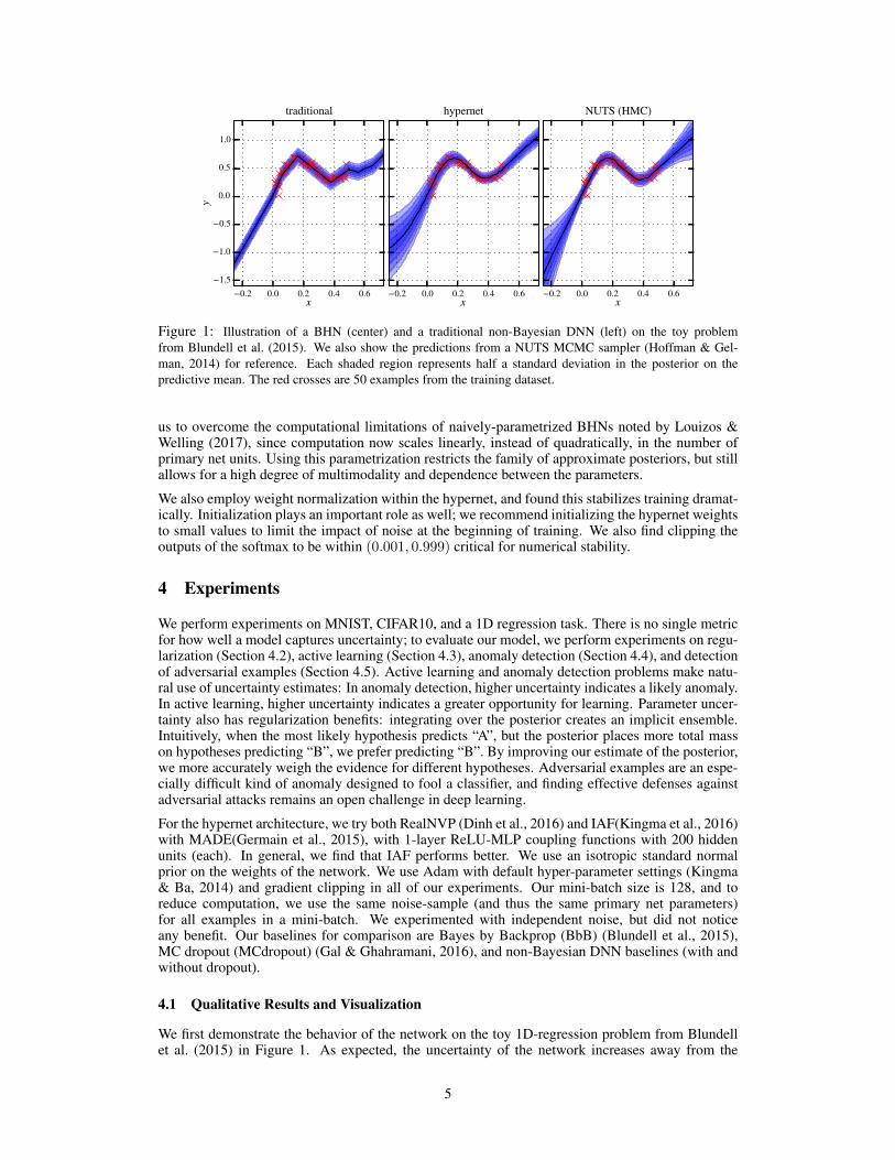
Figure 1: Illustration of a BHN (center) and a traditional non-Bayesian DNN (left) on the toy problemfrom Blundell et al. (2015). We also show the predictions from a NUTS MCMC sampler (Hoffman & Gel-man, 2014) for reference. Each shaded region represents half a standard deviation in the posterior on thepredictive mean. The red crosses are 50 examples from the training dataset.
us to overcome the computational limitations of naively-parametrized BHNs noted by Louizos &Welling (2017), since computation now scales linearly, instead of quadratically, in the number ofprimary net units. Using this parametrization restricts the family of approximate posteriors, but stillallows for a high degree of multimodality and dependence between the parameters.
We also employ weight normalization within the hypernet, and found this stabilizes training dramat-ically. Initialization plays an important role as well; we recommend initializing the hypernet weightsto small values to limit the impact of noise at the beginning of training. We also find clipping theoutputs of the softmax to be within (0.001, 0.999) critical for numerical stability.
4 Experiments
We perform experiments on MNIST, CIFAR10, and a 1D regression task. There is no single metricfor how well a model captures uncertainty; to evaluate our model, we perform experiments on regu-larization (Section 4.2), active learning (Section 4.3), anomaly detection (Section 4.4), and detectionof adversarial examples (Section 4.5). Active learning and anomaly detection problems make natu-ral use of uncertainty estimates: In anomaly detection, higher uncertainty indicates a likely anomaly.In active learning, higher uncertainty indicates a greater opportunity for learning. Parameter uncer-tainty also has regularization benefits: integrating over the posterior creates an implicit ensemble.Intuitively, when the most likely hypothesis predicts “A”, but the posterior places more total masson hypotheses predicting “B”, we prefer predicting “B”. By improving our estimate of the posterior,we more accurately weigh the evidence for different hypotheses. Adversarial examples are an espe-cially difficult kind of anomaly designed to fool a classifier, and finding effective defenses againstadversarial attacks remains an open challenge in deep learning.
For the hypernet architecture, we try both RealNVP (Dinh et al., 2016) and IAF(Kingma et al., 2016)with MADE(Germain et al., 2015), with 1-layer ReLU-MLP coupling functions with 200 hiddenunits (each). In general, we find that IAF performs better. We use an isotropic standard normalprior on the weights of the network. We use Adam with default hyper-parameter settings (Kingma& Ba, 2014) and gradient clipping in all of our experiments. Our mini-batch size is 128, and toreduce computation, we use the same noise-sample (and thus the same primary net parameters)for all examples in a mini-batch. We experimented with independent noise, but did not noticeany benefit. Our baselines for comparison are Bayes by Backprop (BbB) (Blundell et al., 2015),MC dropout (MCdropout) (Gal & Ghahramani, 2016), and non-Bayesian DNN baselines (with andwithout dropout).
4.1 Qualitative Results and Visualization
We first demonstrate the behavior of the network on the toy 1D-regression problem from Blundellet al. (2015) in Figure 1. As expected, the uncertainty of the network increases away from the
5

2 0 2a
3
2
1
0
1
2
3
b
hypernet
2 0 2a
NUTS (HMC)
Figure 2: Learning the identity function with an overparametrized network: y = a · b · x. This parametriza-tion results in symmetries shown by the dashed red lines, and the Bayesian hypernetwork assigns significantprobability mass to both modes of the posterior (a = b = 1 and a = b = −1).
observed data, although the model still suffers from overconfidence to some extent compared withHamiltonian Monte Carlo (Neal et al., 2011), which excels on low-dimensional problems. Next, wedemonstrate the distinctive ability of Bayesian hypernets to learn multi-modal, dependent distribu-tions. Figure 6 (appendix) shows that BHNs do learn approximate posteriors with dependence be-tween different parameters, as measured by the Pearson correlation coefficient. Meanwhile, Figure 2shows that BHNs are capable of learning multimodal posteriors. For this experiment, we trained anover-parametrized linear (primary) network: y = a · b · x on a dataset generated as y = x + ε, andthe BHN learns capture both the modes of a = b = 1 and a = b = −1.
4.2 Classification
dropout BHN (IAF) BHN (RNVP)95.0
95.2
95.4
95.6
95.8
96.0
96.2
96.4
accu
racy
(%)
Figure 3: Box plot of performance across10 trials. Bayesian hypernets (BHNs) withinverse autoregressive flows (IAF) consis-tently outperform the other methods.
We now show that BHNs act as a regularizer, outperform-ing dropout and traditional mean field (BbB). Results arepresented in Table 1. In our experiments, we find thatBHNs perform on par with dropout on full datasets ofMNIST and CIFAR10; furthermore, increasing the flex-ibility of the posterior by adding more coupling layersimproves performance, especially compared with modelswith 0 coupling layers, which cannot model dependenciesbetween the parameters. We also evaluate on a subset ofMNIST (the first 5,000 examples); results are presentedin the last two columns of Table 1. Replicating these ex-periments (with 8 coupling layers) for 10 trials yields Fig-ure 3.
In these MNIST experiments, we use MLPs with 2 hiddenlayers of 800 or 1200 hidden units each. For CIFAR10,we train a convolutional neural net (CNN) with 4 hiddenlayers of [64, 64, 128, 128] channels, 2 × 2 max poolingafter the second and the fourth layers, filter size of 3, anda single fully connected layer of 512 units.
4.3 Active Learning
We now turn to active learning, where we compare to the MNIST experiments of Gal et al. (2017),replicating their architecture and training procedure. Briefly, they use an initial dataset of 20 exam-ples (2 from each class), and acquire 10 new examples at a time, training for 50 epochs betweeneach acquisition. While Gal et al. (2017) re-initialize the network after every acquisition, we found
6

Table 1: Generalization results on MNIST and CIFAR10 for BHNs with different numbers of RealNVP cou-pling layers (#), and comparison methods (dropout / maximum likelihood (MLE)). Bayes-by-backprop (Blun-dell et al., 2015) (*) models each parameter as an independent Gaussian, which is equivalent to using a hypernetwith 0 coupling layers. We achieved a better result outputting a distribution over scaling factors (only). MNIST5000 (A) and (B) are generalization results on subset (5,000 training data) of MNIST, (A) MLP with 800 hiddennodes. (B) MLP with 1,200 hidden nodes.
MNIST 50,000 CIFAR10 50,000 MNIST 5,000 (A) MNIST 5,000 (B)
# Accuracy # Accuracy # Accuracy # Accuracy
0 98.28% (98.01%*) 0 67.83% 0 92.06% 0 90.91%2 98.39% 4 74.77% 8 94.25% 8 96.27%4 98.47% 8 74.90% 12 96.16% 12 96.51%6 98.59% dropout 74.08% dropout 95.58% dropout 95.52%8 98.63% MLE 72.75%
dropout 98.73%
Figure 4: Active learning: Bayesian hypernets outperform other approaches after sufficient acqui-sitions when warm-starting (left), for both random acquisition function (top) and BALD acquisitionfunction (bottom). Warm-starting improves stability for all methods, but hurts performance for otherapproaches, compared with randomly re-initializing parameters as in Gal et al. (2017) (right). Wealso note that the baseline model (no dropout) is competitive with MCdropout, and outperforms theDropout baseline used by (Gal et al., 2017).8 These curves are the average of three experiments.
that “warm-starting” from the current learned parameters was essential for good performance withBHNs, although it is likely that longer training or better initialization schemes could perform thesame role. Overall, warm-started BHNs suffered at the beginning of training, but outperformed allother methods for moderate to large numbers of acquisitions.
7

Table 2: Anomaly detection on MNIST. Since we use the same datasets as Hendrycks & Gimpel (2016), wehave the same base error rates, and refer the reader to that work.
Dataset MLP MC dropout BHN
ROC PR(+) PR(−) ROC PR(+) PR(−) ROC PR(+) PR(−)
Uniform 96.99 97.99 94.71 98.90 99.15 98.63 98.97 99.27 98.52OmniGlot 94.92 95.63 93.85 95.87 96.44 94.84 94.89 95.56 93.64CIFARbw 95.55 96.47 93.72 98.70 98.98 98.39 96.63 97.25 95.78Gaussian 87.70 87.66 88.05 97.70 98.11 96.94 89.22 86.62 89.85notMNIST 81.12 97.56 39.70 97.78 99.78 78.53 90.07 98.51 56.59
4.4 Anomaly Detection
For anomaly detection, we take Hendrycks & Gimpel (2016) as a starting point, and perform thesame suite of MNIST experiments, evaluating the ability of networks to determine whether an inputcame from their training distribution (“Out of distribution detection”). Hendrycks & Gimpel (2016)found that the confidence expressed in the softmax probabilities of a (non-Bayesian) DNN trainedon a single dataset provides a good signal for both of these detection problems. We demonstrate thatBayesian DNNs outperform their non-Bayesian counterparts.
Just as in active learning, in anomaly detection, we use MC to estimate the predictive posterior, anduse this to score datapoints. For active learning, we would generally like to acquire points wherethere is higher uncertainty. In a well-calibrated model, these points are also likely to be challengingor anomalous examples, and thus acquisition functions from the active learning literature are goodcandidates for scoring anomalies.
We consider all of the acquisition functions listed in (Gal et al., 2017) as possible scores for theArea Under the Curve (AUC) of Precision-Recall (PR) and Receiver Operating Characteristic (ROC)metrics, but found that the maximum confidence of the softmax probabilities (i.e., “variation ratio”)acquisition function used by Hendrycks & Gimpel (2016) gave the best performance. Both BHN andMCdropout achieve significant performance gains over the non-Bayesian baseline, and MCdropoutperforms significantly better than BHN in this task. Results are presented in Table 2.
Second, we follow the same experimental setup, using all the acquisition functions, and excludeone class in the training set of MNIST at a time. We take the excluded class of the training data asout-of-distribution samples. The result is presented in Table 3 (Appendix). This experiment showsthe benefit of using scores that reflect dispersion in the posterior samples (such as mean standarddeviation and BALD value) in Bayesian DNNs.
4.5 Adversary Detection
Finally, we consider this same anomaly detection procedure as a novel tool for detecting adversarialexamples. Our setup is similar to Li & Gal (2017) and Louizos & Welling (2017), where it is shownthat when more perturbation is added to the data, model uncertainty increases and then drops. Weuse the Fast Gradient Sign method (FGS) (Goodfellow et al., 2014b) for adversarial attack, and useone sample of our model to estimate the gradient.9 We find that, compared with dropout, BHNs areless confident on data points which are far from the data manifold. In particular, BHNs constructedwith IAF consistently outperform RealNVP-BHNs and dropout in detecting adversarial examplesand errors. Results are shown in Figure 5.
8For the deterministic baseline, the value of the BALD acquisition function is always zero, and so acquisi-tions should be random, but due to numerical instability this is not the case in our implementation; surprisingly,we found the BALD values our implementation computes provide a better-than-random acquisition function(compare the blue line in the top and bottom plots).
9 Li & Gal (2017) and Louizos & Welling (2017) used 10 and 1 model samples, respectively, to estimategradient. We report the result with 1 sample; results with more samples are given in the appendix.
8

0.00 0.25 0.50
0.0
0.2
0.4
0.6
0.8
1.0
(%)
Accuracy
0.00 0.25 0.500.00
0.05
0.10
0.15
0.20
Aver
age
Scor
e
BALD
0.00 0.25 0.500.10
0.15
0.20
0.25
0.30
0.35
Entropy
0.00 0.25 0.50
0.025
0.050
0.075
0.100
0.125Variation Ratio
0.00 0.25 0.50
0.01
0.02
0.03
0.04Mean STD
0.00 0.25 0.500.5
0.6
0.7
0.8
Adve
rsar
y De
tect
ion
0.00 0.25 0.500.5
0.6
0.7
0.8
0.00 0.25 0.500.5
0.6
0.7
0.8
0.00 0.25 0.500.5
0.6
0.7
0.8
0.00 0.25 0.50
0.2
0.4
0.6
0.8
1.0
Erro
r Det
ectio
n
0.00 0.25 0.50
0.2
0.4
0.6
0.8
1.0
0.00 0.25 0.50
0.2
0.4
0.6
0.8
1.0
0.00 0.25 0.50
0.2
0.4
0.6
0.8
1.0
BHN (IAF)BHN (RNVP)dropout
0.0 0.2 0.4 0.6 0.8 1.0step size
0.0
0.2
0.4
0.6
0.8
1.0
Figure 5: Adversary detection: Horizontal axis is the step size of the FGS algorithm. While accuracy dropswhen more perturbation is added to the data (left), uncertainty measures also increase (first row). In particular,the BALD and Mean STD scores, which measure epistemic uncertainty, are strongly increasing for BHNs, butnot for dropout. The second row and third row plots show results for adversary detection and error detection(respectively) in terms of the AUC of ROC (y-axis) with increasing perturbation along the x-axis. Gradientdirection is estimated with one Monte Carlo sample of the weights/dropout mask.
5 Conclusions
We introduce Bayesian hypernets (BHNs), a new method for variational Bayesian deep learningwhich uses an invertible hypernetwork as a generative model of parameters. BHNs feature efficienttraining and sampling, and can express complicated multimodal distributions, thereby addressingissues of overconfidence present in simpler variational approximations. We present a method ofparametrizing BHNs which allows them to scale successfully to real world tasks, and show thatBHNs can offer significant benefits over simpler methods for Bayesian deep learning. Future workcould explore other methods of parametrizing BHNs, for instance using the same hypernet to outputdifferent subsets of the primary net parameters.
ReferencesDario Amodei, Chris Olah, Jacob Steinhardt, Paul Christiano, John Schulman, and Dan Mane. Con-
crete problems in AI safety. CoRR, abs/1606.06565, 2016. URL http://arxiv.org/abs/1606.06565.
Luca Bertinetto, Joao F. Henriques, Jack Valmadre, Philip H. S. Torr, and Andrea Vedaldi. Learningfeed-forward one-shot learners. CoRR, abs/1606.05233, 2016. URL http://arxiv.org/abs/1606.05233.
Charles Blundell, Julien Cornebise, Koray Kavukcuoglu, and Daan Wierstra. Weight uncertainty inneural networks. In Proceedings of The 32nd International Conference on Machine Learning, pp.1613–1622, 2015.
Bert De Brabandere, Xu Jia, Tinne Tuytelaars, and Luc Van Gool. Dynamic filter networks. CoRR,abs/1605.09673, 2016. URL http://arxiv.org/abs/1605.09673.
Nicholas Carlini and David Wagner. Adversarial examples are not easily detected: Bypassing tendetection methods. arXiv preprint arXiv:1705.07263, 2017.
9

Laurent Dinh, David Krueger, and Yoshua Bengio. NICE: Non-linear independent componentsestimation. arXiv preprint arXiv:1410.8516, 2014.
Laurent Dinh, Jascha Sohl-Dickstein, and Samy Bengio. Density estimation using real NVP. arXivpreprint arXiv:1605.08803, 2016.
Vincent Dumoulin, Jonathon Shlens, and Manjunath Kudlur. A learned representation for artisticstyle. CoRR, abs/1610.07629, 2016. URL http://arxiv.org/abs/1610.07629.
Yarin Gal. Uncertainty in deep learning. 2016.
Yarin Gal and Zoubin Ghahramani. Dropout as a Bayesian approximation: Representing modeluncertainty in deep learning. In International Conference on Machine Learning, pp. 1050–1059,2016.
Yarin Gal, Riashat Islam, and Zoubin Ghahramani. Deep Bayesian active learning with image data.In Proceedings of the 34th International Conference on Machine Learning, ICML 2017, Sydney,NSW, Australia, 6-11 August 2017, pp. 1183–1192, 2017. URL http://proceedings.mlr.press/v70/gal17a.html.
Mathieu Germain, Karol Gregor, Iain Murray, and Hugo Larochelle. MADE: masked autoencoderfor distribution estimation. In Proceedings of the 32nd International Conference on MachineLearning (ICML-15), pp. 881–889, 2015.
Ian J. Goodfellow. NIPS 2016 tutorial: Generative adversarial networks. CoRR, abs/1701.00160,2017. URL http://arxiv.org/abs/1701.00160.
Ian J. Goodfellow, Jean Pouget-Abadie, Mehdi Mirza, Bing Xu, David Warde-Farley, Sherjil Ozair,Aaron C. Courville, and Yoshua Bengio. Generative adversarial nets. In Advances in Neu-ral Information Processing Systems 27: Annual Conference on Neural Information ProcessingSystems 2014, December 8-13 2014, Montreal, Quebec, Canada, pp. 2672–2680, 2014a. URLhttp://papers.nips.cc/paper/5423-generative-adversarial-nets.
Ian J. Goodfellow, Jonathon Shlens, and Christian Szegedy. Explaining and harnessing adversarialexamples. arXiv preprint arXiv:1412.6572, 2014b.
Ian J. Goodfellow, Yoshua Bengio, and Aaron Courville. Deep Learning. MIT Press, 2016. URLhttp://www.deeplearningbook.org.
Alex Graves. Practical variational inference for neural networks. In J. Shawe-Taylor, R. S. Zemel,P. L. Bartlett, F. Pereira, and K. Q. Weinberger (eds.), Advances in Neural Information ProcessingSystems 24, pp. 2348–2356. Curran Associates, Inc., 2011. URL http://papers.nips.cc/paper/4329-practical-variational-inference-for-neural-networks.pdf.
David Ha, Andrew Dai, and Quoc V. Le. Hypernetworks. 2017. URL https://openreview.net/pdf?id=rkpACe1lx.
Dan Hendrycks and Kevin Gimpel. A baseline for detecting misclassified and out-of-distributionexamples in neural networks. arXiv preprint arXiv:1610.02136, 2016.
Jose Miguel Hernandez-Lobato and Ryan Adams. Probabilistic backpropagation for scalable learn-ing of Bayesian neural networks. In Proceedings of The 32nd International Conference on Ma-chine Learning, pp. 1861–1869, 2015.
Matthew D. Hoffman and Andrew Gelman. The No-U-Turn Sampler: Adaptively setting pathlengths in Hamiltonian Monte Carlo. Journal of Machine Learning Research, 15(1):1593–1623,2014.
Xun Huang and Serge J. Belongie. Arbitrary style transfer in real-time with adaptive instance nor-malization. CoRR, abs/1703.06868, 2017. URL http://arxiv.org/abs/1703.06868.
D. Jimenez Rezende, S. Mohamed, and D. Wierstra. Stochastic backpropagation and approximateinference in deep generative models. arXiv e-prints, January 2014.
10
Diederik P. Kingma and Jimmy Ba. Adam: A method for stochastic optimization. CoRR,abs/1412.6980, 2014. URL http://arxiv.org/abs/1412.6980.
Diederik P. Kingma and Max Welling. Auto-encoding variational Bayes. arXiv preprintarXiv:1312.6114, 2013.
Diederik. P. Kingma, T. Salimans, and M. Welling. Variational Dropout and the Local Reparame-terization Trick. arXiv e-prints, June 2015.
Diederik P. Kingma, Tim Salimans, Rafal Jozefowicz, Xi Chen, Ilya Sutskever, and Max Welling.Improved variational inference with inverse autoregressive flow. In Advances in Neural Informa-tion Processing Systems, pp. 4743–4751, 2016.
James Kirkpatrick, Razvan Pascanu, Neil C. Rabinowitz, Joel Veness, Guillaume Desjardins, An-drei A. Rusu, Kieran Milan, John Quan, Tiago Ramalho, Agnieszka Grabska-Barwinska, DemisHassabis, Claudia Clopath, Dharshan Kumaran, and Raia Hadsell. Overcoming catastrophic for-getting in neural networks. CoRR, abs/1612.00796, 2016. URL http://arxiv.org/abs/1612.00796.
Yingzhen Li and Yarin Gal. Dropout inference in Bayesian neural networks with alpha-divergences.arXiv preprint arXiv:1703.02914, 2017.
Christos Louizos and Max Welling. Multiplicative normalizing flows for variational bayesian neuralnetworks. arXiv e-prints, March 2017.
David J.C. MacKay. Bayesian neural networks and density networks. In Nuclear Instruments andMethods in Physics Research, A, pp. 73–80, 1994.
Radford M. Neal. Bayesian Learning for Neural Networks. Springer-Verlag New York, Inc., Secau-cus, NJ, USA, 1996. ISBN 0387947248.
Radford M. Neal et al. MCMC using Hamiltonian dynamics. Handbook of Markov Chain MonteCarlo, 2(11), 2011.
Ethan Perez, Harm de Vries, Florian Strub, Vincent Dumoulin, and Aaron C. Courville. Learningvisual reasoning without strong priors. CoRR, abs/1707.03017, 2017. URL http://arxiv.org/abs/1707.03017.
Danilo Rezende and Shakir Mohamed. Variational inference with normalizing flows. In Proceedingsof The 32nd International Conference on Machine Learning, pp. 1530–1538, 2015.
Tim Salimans and Diederik P. Kingma. Weight normalization: A simple reparameterization toaccelerate training of deep neural networks. CoRR, abs/1602.07868, 2016. URL http://arxiv.org/abs/1602.07868.
Tim Salimans, Diederik P. Kingma, and Max Welling. Markov chain Monte Carlo and variationalinference: Bridging the gap. In Proceedings of the 32nd International Conference on MachineLearning (ICML-15), pp. 1218–1226, 2015.
Jiaxin Shi, Shengyang Sun, and Jun Zhu. Implicit variational inference with kernel density ratiofitting. arXiv preprint arXiv:1705.10119, 2017.
Daniel Soudry, Itay Hubara, and Ron Meir. Expectation backpropagation: Parameter-free train-ing of multilayer neural networks with continuous or discrete weights. In Advances in NeuralInformation Processing Systems, pp. 963–971, 2014.
Nitish Srivastava, Geoffrey Hinton, Alex Krizhevsky, Ilya Sutskever, and Ruslan Salakhutdinov.Dropout: A simple way to prevent neural networks from overfitting. J. Mach. Learn. Res., 15(1):1929–1958, January 2014. ISSN 1532-4435. URL http://dl.acm.org/citation.cfm?id=2627435.2670313.
Dmitry Ulyanov, Andrea Vedaldi, and Victor S. Lempitsky. Instance normalization: The missingingredient for fast stylization. CoRR, abs/1607.08022, 2016. URL http://arxiv.org/abs/1607.08022.
Max Welling and Yee Whye Teh. Bayesian learning via stochastic gradient Langevin dynamics,2011.
11
A Additional Results
A.1 Learning correlated weights
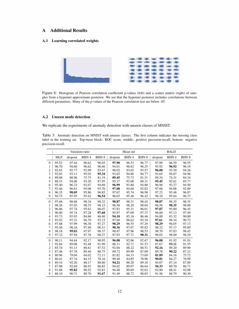
Figure 6: Histogram of Pearson correlation coefficient p-values (left) and a scatter matrix (right) of sam-ples from a hypernet approximate posterior. We see that the hypernet posterior includes correlations betweendifferent parameters. Many of the p-values of the Pearson correlation test are below .05.
A.2 Unseen mode detection
We replicate the experiments of anomaly detection with unseen classes of MNIST.
Table 3: Anomaly detection on MNIST with unseen classes. The first column indicates the missing classlabel in the training set. Top-most block: ROC score; middle: positive precision-recall; bottom: negativeprecision-recall.
Variation ratio Mean std BALD
MLP dropout BHN 4 BHN 8 dropout BHN 4 BHN 8 dropout BHN 4 BHN 8
0 95.52 97.44 96.62 96.45 97.90 96.53 96.77 97.89 96.59 96.551 96.70 94.60 96.62 96.46 94.01 96.62 96.25 93.92 96.92 96.192 92.83 95.77 92.99 93.47 96.02 93.03 93.57 96.08 93.59 94.263 93.03 93.11 95.03 95.34 93.65 94.86 94.77 93.65 94.87 94.964 89.08 88.96 75.73 81.19 89.45 75.73 81.31 89.34 74.31 84.345 88.53 94.66 93.20 87.95 95.37 93.08 88.31 95.45 92.61 85.776 95.40 96.33 93.67 94.69 96.99 93.80 94.80 96.96 93.27 94.507 92.46 96.61 95.08 93.70 97.08 94.68 92.82 97.06 94.88 92.898 96.35 98.05 95.86 96.85 97.67 95.74 96.98 97.23 95.48 96.879 94.75 95.95 95.62 96.54 96.03 95.46 96.42 96.10 95.84 96.37
0 97.68 98.68 98.34 98.32 98.87 98.31 98.45 98.87 98.35 98.351 98.26 97.03 98.23 98.15 96.58 98.20 98.04 96.58 98.35 98.002 96.06 97.74 95.63 96.07 97.83 95.31 96.01 97.87 95.80 96.453 96.00 95.74 97.28 97.68 95.97 97.09 97.37 96.00 97.13 97.494 93.73 93.93 84.66 86.40 94.10 85.16 86.46 94.00 83.32 90.005 93.92 97.31 96.79 93.15 97.60 96.62 93.34 97.61 96.34 90.726 97.68 97.99 96.38 97.27 98.29 96.55 97.29 98.29 96.05 97.137 95.56 98.16 97.40 96.51 98.36 97.07 95.82 98.32 97.17 95.898 98.18 99.03 97.97 98.37 98.87 97.96 98.53 98.70 97.83 98.459 97.32 97.94 97.76 98.27 97.93 97.71 98.31 98.02 98.00 98.29
0 90.11 94.44 92.17 90.95 96.08 92.06 92.67 96.08 91.92 91.911 92.84 89.08 92.48 91.99 88.11 92.71 91.53 87.67 93.11 91.552 85.74 91.13 86.61 87.52 92.04 88.22 88.51 92.16 89.20 89.903 87.46 87.78 89.46 88.75 89.72 89.99 87.09 89.78 90.22 87.214 80.96 79.04 64.02 72.11 81.82 64.33 73.69 81.89 64.16 75.725 80.41 87.74 84.15 78.16 90.48 84.85 78.96 90.81 84.27 76.996 89.34 92.26 88.17 88.60 94.21 88.28 89.10 94.07 87.14 87.897 87.08 92.69 88.91 86.85 94.02 89.07 86.64 94.33 89.70 86.718 91.88 95.82 90.52 92.83 94.40 89.69 92.82 92.80 88.41 92.089 88.10 90.71 89.70 91.67 91.49 88.72 90.85 91.56 88.79 90.30
12

A.3 Stronger attack
Here we use 32 samples to estimate the gradient direction with respect to the input. A better estimateof gradient amounts to a stronger attack, so accuracy drops lower for a given step size while anadversarial example can be more easily detected with a more informative uncertainty measure.
0.00 0.25 0.50
0.0
0.2
0.4
0.6
0.8
1.0
(%)
Accuracy
0.00 0.25 0.500.00
0.05
0.10
0.15
0.20
Aver
age
Scor
e
BALD
0.00 0.25 0.500.1
0.2
0.3
0.4Entropy
0.00 0.25 0.50
0.025
0.050
0.075
0.100
0.125
Variation Ratio
0.00 0.25 0.50
0.01
0.02
0.03
0.04Mean STD
0.00 0.25 0.500.5
0.6
0.7
0.8
Adve
rsar
y De
tect
ion
0.00 0.25 0.500.5
0.6
0.7
0.8
0.00 0.25 0.500.5
0.6
0.7
0.8
0.00 0.25 0.500.5
0.6
0.7
0.8
0.00 0.25 0.50
0.2
0.4
0.6
0.8
1.0
Erro
r Det
ectio
n
0.00 0.25 0.50
0.2
0.4
0.6
0.8
1.0
0.00 0.25 0.50
0.2
0.4
0.6
0.8
1.0
0.00 0.25 0.50
0.2
0.4
0.6
0.8
1.0
BHN (IAF)BHN (RNVP)dropout
0.0 0.2 0.4 0.6 0.8 1.0step size
0.0
0.2
0.4
0.6
0.8
1.0
Figure 7: Adversary detection with 32-sample estimate of gradient.
13