1

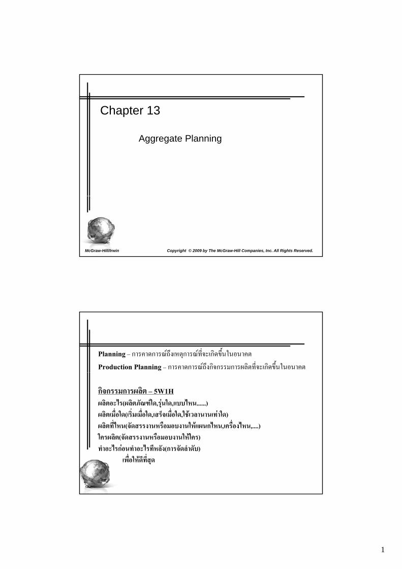
Chapter 13

A t Pl iAggregate Planning

McGraw-Hill/Irwin Copyright © 2009 by The McGraw-Hill Companies, Inc. All Rights Reserved.

Planning – การคาดการณถึงเหตุการณที่จะเกิดขึ้นในอนาคตProduction Planning – การคาดการณถึงกิจกรรมการผลิตที่จะเกิดขึ้นในอนาคต

กิจกรรมการผลิต – 5W1Hผลิตอะไร(ผลิตภัณฑใด,รุนใด,แบบไหน......)ผลิตเม่ือใด(เร่ิมเม่ือใด,เสร็จเม่ือใด,ใชเวลานานเทาใด)ผลิตท่ีไหน(จัดสรรงานหรือมอบงานใหแผนกไหน,เคร่ืองไหน,....)ใ ื ใ ใใครผลิต(จัดสรรงานหรือมอบงานใหใคร)ทําอะไรกอนทําอะไรทีหลัง(การจัดลําดับ)

เพ่ือใหดีท่ีสุด

2

Aggregate Planning

• Aggregate planning– Intermediate-range capacity planning that typically– Intermediate-range capacity planning that typically

covers a time horizon of 2 to 18 months– Useful for organizations that experience seasonal, or

other variations in demand– Goal:

• Achieve a production plan that will effectively utilize the organi ations’ reso rces to satisf demandorganizations’ resources to satisfy demand

Sales and Operations Planning

• Some organizations use the term sales and operations planning rather than aggregateoperations planning rather than aggregate planning– Sales and operation planning

• Intermediate-range planning decisions to balance supply and demand, integrating financial and operations planning

• Since the plan affects functions throughout the• Since the plan affects functions throughout the organization, it is typically prepared with inputs from sales, finance, and operations

3

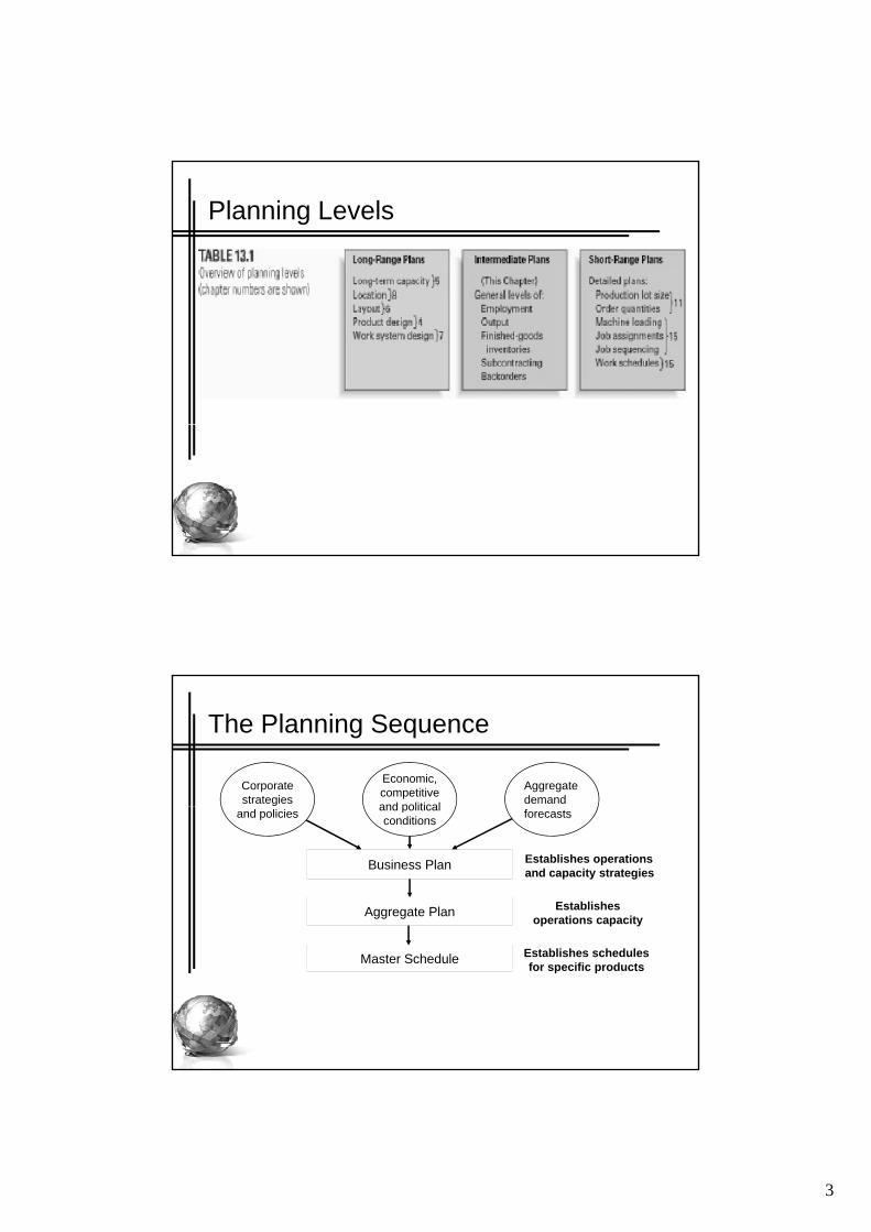
Planning Levels

The Planning Sequence

Corporatestrategies

Economic,competitiveand political

Aggregate demand

Business Plan Establishes operationsand capacity strategies

Aggregate Plan Establishesoperations capacity

and policies and politicalconditions forecasts

Master Schedule Establishes schedulesfor specific products

4

Aggregation

• The plan must be in units of measurement that can be understood by the firm’s non-operations personnely p p

• Aggregate units of output per month

• Dollar value of total monthly output

• Total output by factory

• Measures that relate to capacity such as labor hours

Dealing with Variation

• Most organizations use rolling 3, 6, 9 and 12 month forecastsmonth forecasts– Forecasts are updated periodically, rather than relying

on a once-a-year forecast

5

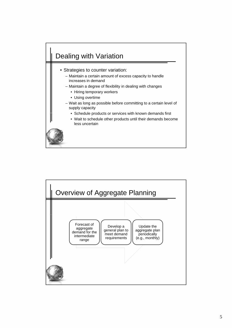
Dealing with Variation

• Strategies to counter variation:– Maintain a certain amount of excess capacity to handle p y

increases in demand– Maintain a degree of flexibility in dealing with changes

• Hiring temporary workers• Using overtime

– Wait as long as possible before committing to a certain level of supply capacity• Schedule products or services with known demands first• Schedule products or services with known demands first• Wait to schedule other products until their demands become

less uncertain

Overview of Aggregate Planning

Forecast of aggregate

demand for the intermediate

range

Develop a general plan to meet demand requirements

Update the aggregate plan

periodically (e.g., monthly)

6

Demand and Supply

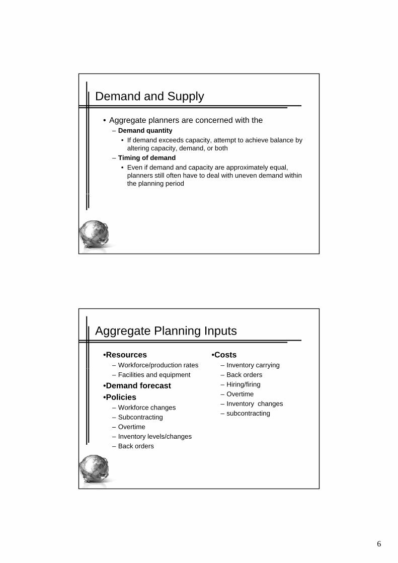
• Aggregate planners are concerned with the– Demand quantityq y

• If demand exceeds capacity, attempt to achieve balance by altering capacity, demand, or both

– Timing of demand• Even if demand and capacity are approximately equal,

planners still often have to deal with uneven demand within the planning period

Aggregate Planning Inputs

•Resources– Workforce/production rates

•Costs– Inventory carryingp

– Facilities and equipment

•Demand forecast•Policies

– Workforce changes– Subcontracting– Overtime

y y g– Back orders– Hiring/firing– Overtime– Inventory changes– subcontracting

Overtime– Inventory levels/changes– Back orders

7

Aggregate Planning Outputs

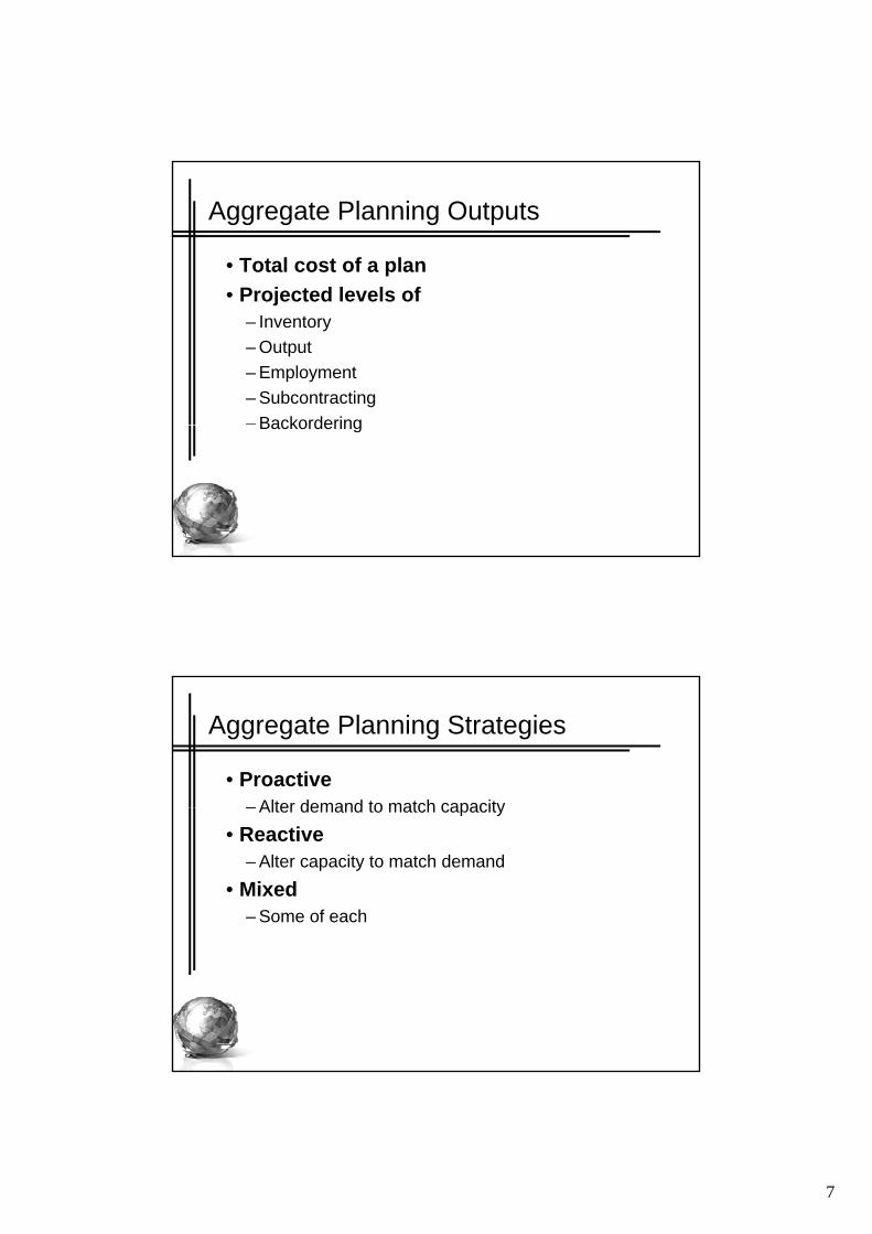
• Total cost of a plan• Projected levels of• Projected levels of

– Inventory– Output– Employment– Subcontracting– BackorderingBackordering

Aggregate Planning Strategies

• Proactive– Alter demand to match capacity– Alter demand to match capacity

• Reactive– Alter capacity to match demand

• Mixed– Some of each

8

Demand Options

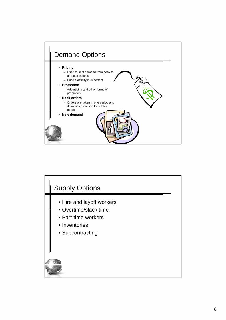
• Pricing– Used to shift demand from peak to

off-peak periodsoff-peak periods– Price elasticity is important

• Promotion– Advertising and other forms of

promotion• Back orders

– Orders are taken in one period and deliveries promised for a later periodperiod

• New demand

Supply Options

• Hire and layoff workers• Overtime/slack time• Overtime/slack time• Part-time workers• Inventories• Subcontracting

9

Aggregate Planning Pure Strategies

• Level capacity strategy: – Maintaining a steady rate of regular-time output whileMaintaining a steady rate of regular time output while

meeting variations in demand by a combination of options: • inventories, overtime, part-time workers, subcontracting,

and back orders• Chase demand strategy:

– Matching capacity to demand; the planned output for a period is set at the expected demand for that period.

Chase Approach

• Capacities are adjusted to match demand requirements over the planning horizonrequirements over the planning horizon– Advantages

• Investment in inventory is low• Labor utilization in high

– Disadvantages• The cost of adjusting output rates and/or workforce

levels

10

Level Approach

• Capacities are kept constant over the planning horizonhorizon

• Advantages– Stable output rates and workforce

• Disadvantages– Greater inventory costs

Increased overtime and idle time– Increased overtime and idle time– Resource utilizations vary over time

Techniques for Aggregate Planning

• General procedure:1 Determine demand for each period1.Determine demand for each period

2.Determine capacities for each period

3.Identify company or departmental policies that are pertinent

4.Determine unit costs

5.Develop alternative plans and costs

6 Select the plan that best satisfies objectives Otherwise return to6.Select the plan that best satisfies objectives. Otherwise return to step 5.

11

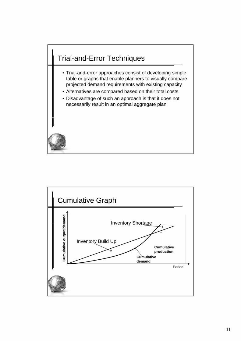
Trial-and-Error Techniques

• Trial-and-error approaches consist of developing simple table or graphs that enable planners to visually compare g p p y pprojected demand requirements with existing capacity

• Alternatives are compared based on their total costs• Disadvantage of such an approach is that it does not

necessarily result in an optimal aggregate plan

Cumulative Graph

man

d

Inventory Shortage

Cumulativeproduction

Cumulative

Cum

ulat

ive

outp

ut/d

em

Inventory Build Up

Inventory Shortage

demandC

Period

12

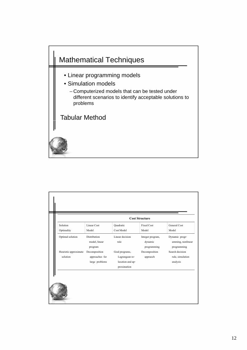
Mathematical Techniques

• Linear programming models• Simulation models• Simulation models

– Computerized models that can be tested under different scenarios to identify acceptable solutions to problems

Tabular Method

Cost StructureSolution Linear Cost Quadratic Fixed Cost General CostOptimality Model Cost Model Model Model

Optimal solution

Heuristic approximate solution

Distributionmodel, linearprogram

Decompositionapproaches for large problems

Linear decisionrule

Goal programs,Lagrangean re-laxation and ap-proximation

Integer program,dynamic programming

Decompositionappraoch

Dynamic progr-amming, nonlinear programming

Search decisionrule, simulationanalysis

proximation

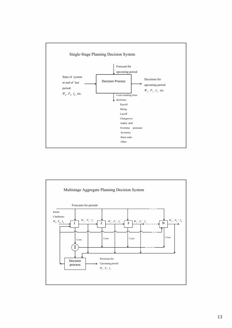
13

Single-Stage Planning Decision System

Forecast for upcoming period

State of system Decision Process

yat end of last period:W0 , P0 , I0 , etc.

Decisions for upcoming period W1 , P1 , I1 , etc.

Costs resulting from decisions:

PayrollHiringL ffLayoffChangeoverAdded shiftOvertime premiumInventoryBack orderOther

Multistage Aggregate Planning Decision System

Forecasts for periodsInitial

WN’ , PN’ , IN

’

1 2 3 N

Σ

Costs Costs Costs Costs

W2’ , P2’ , I2

’W1’ , P1’ , I1

’W3

’ , P3’ , I3’

Cinditions:W0 , P0 , I0

Decision process

Decisions forUpcoming period:W1 , P1 , I1

14

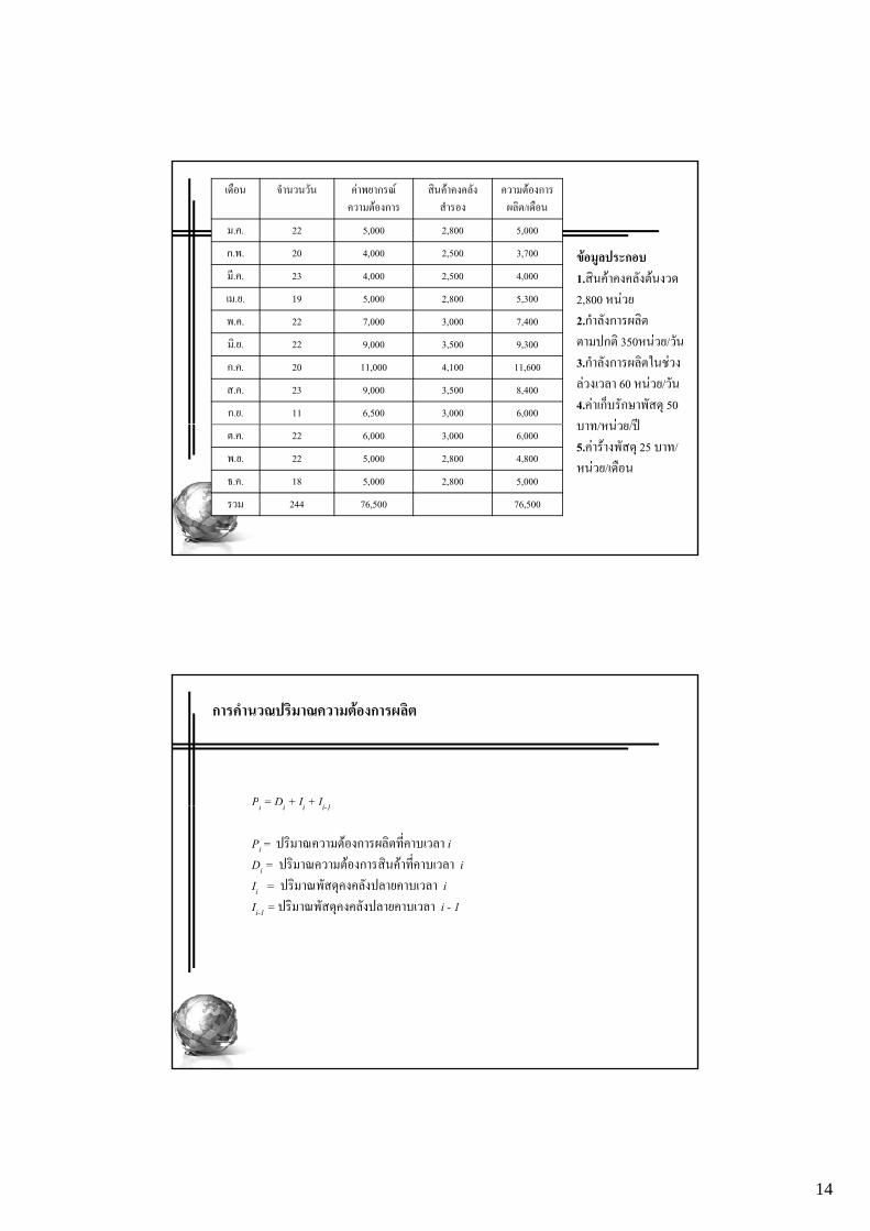
เดือน จํานวนวัน คาพยากรณ ความตองการ

สินคาคงคลังสํารอง

ความตองการผลิต/เดือน

ม.ค. 22 5,000 2,800 5,000

ก.พ. 20 4,000 2,500 3,700

มี.ค. 23 4,000 2,500 4,000ขอมูลประกอบ1.สินคาคงคลังตนงวด

เม.ย. 19 5,000 2,800 5,300

พ.ค. 22 7,000 3,000 7,400

มิ.ย. 22 9,000 3,500 9,300

ก.ค. 20 11,000 4,100 11,600

ส.ค. 23 9,000 3,500 8,400

ก.ย. 11 6,500 3,000 6,000

2,800 หนวย2.กําลังการผลิตตามปกติ 350หนวย/วัน3.กําลังการผลิตในชวงลวงเวลา 60 หนวย/วัน4.คาเก็บรักษาพัสดุ 50 บาท/หนวย/ป

ต.ค. 22 6,000 3,000 6,000

พ.ย. 22 5,000 2,800 4,800

ธ.ค. 18 5,000 2,800 5,000

รวม 244 76,500 76,500

บาท/หนวย/ป5.คารางพัสดุ 25 บาท/หนวย/เดือน

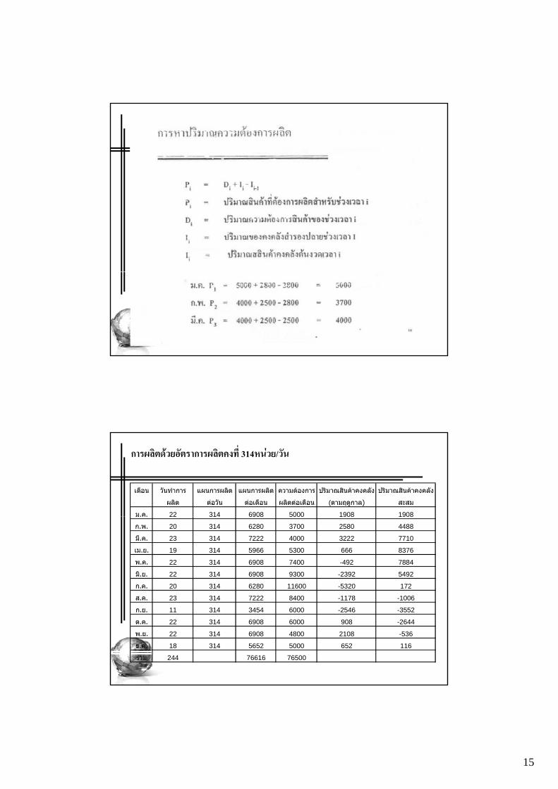
การคํานวณปริมาณความตองการผลิต

Pi = Di + Ii + Ii 1i i i i-1

Pi = ปริมาณความตองการผลิตท่ีคาบเวลา iDi = ปริมาณความตองการสินคาท่ีคาบเวลา iIi = ปริมาณพัสดุคงคลังปลายคาบเวลา iIi-1 = ปริมาณพัสดุคงคลังปลายคาบเวลา i - 1

15

เดือน วันทําการ แผนการผลิต แผนการผลิต ความตองการ ปริมาณสินคาคงคลัง ปริมาณสินคาคงคลัง

ผลิต ตอวัน ตอเดือน ผลิตตอเดือน (ตามฤดูกาล) สะสม

ม.ค. 22 314 6908 5000 1908 1908

การผลิตดวยอัตราการผลิตคงที่ 314หนวย/วัน

ม.ค. 22 314 6908 5000 1908 1908

ก.พ. 20 314 6280 3700 2580 4488

มี.ค. 23 314 7222 4000 3222 7710

เม.ย. 19 314 5966 5300 666 8376

พ.ค. 22 314 6908 7400 -492 7884

มิ.ย. 22 314 6908 9300 -2392 5492

ก.ค. 20 314 6280 11600 -5320 172

ส.ค. 23 314 7222 8400 -1178 -1006

ก.ย. 11 314 3454 6000 -2546 -3552

ต.ค. 22 314 6908 6000 908 -2644

พ.ย. 22 314 6908 4800 2108 -536

ธ.ค. 18 314 5652 5000 652 116

รวม 244 76616 76500

16

เดือน วันทําการ แผนการผลิต แผนการผลิต ความตองการ ปริมาณสินคาคงคลัง ปริมาณสินคาคงคลัง

ผลิต ตอวัน ตอเดือน ผลิตตอเดือน (ตามฤดูกาล) สะสม

การผลิตดวยอัตราการผลิตคงที่ 314หนวย/วันโดยเพ่ิมพัสดุคงคลังตนงวดอีก 3552 หนวย

ม.ค. 22 314 6908 5000 1908 5460

ก.พ. 20 314 6280 3700 2580 8040

มี.ค. 23 314 7222 4000 3222 11262

เม.ย. 19 314 5966 5300 666 11928

พ.ค. 22 314 6908 7400 -492 11436

มิ.ย. 22 314 6908 9300 -2392 9044

ก.ค. 20 314 6280 11600 -5320 3724

ส ค 23 314 7222 8400 1178 2546ส.ค. 23 314 7222 8400 -1178 2546

ก.ย. 11 314 3454 6000 -2546 0

ต.ค. 22 314 6908 6000 908 908

พ.ย. 22 314 6908 4800 2108 3016

ธ.ค. 18 314 5652 5000 652 3668

รวม 244 76616 76500

เดือน วันทําการ แผนการผลิต แผนการผลิต ความตองการ ปริมาณสินคาคงคลัง ปริมาณสินคาคงคลัง

ผลิต ตอวัน ตอเดือน ผลิตตอเดือน (ตามฤดูกาล) สะสม

ม.ค. 22 335 7370 5000 2370 2370

การผลิตดวยอัตราการผลิตคงที่ 335 หนวย/วัน

ก.พ. 20 335 6700 3700 3000 5370

มี.ค. 23 335 7705 4000 3705 9075

เม.ย. 19 335 6365 5300 1065 10140

พ.ค. 22 335 7370 7400 -30 10110

มิ.ย. 22 335 7370 9300 -1930 8180

ก.ค. 20 335 6700 11600 -4900 3280

ส.ค. 23 335 7705 8400 -695 2585

11 335 3685 6000 2315 270ก.ย. 11 335 3685 6000 -2315 270

ต.ค. 22 335 7370 6000 1370 1640

พ.ย. 22 335 7370 4800 2570 4210

ธ.ค. 18 335 6030 5000 1030 5240

รวม 244 81740 76500

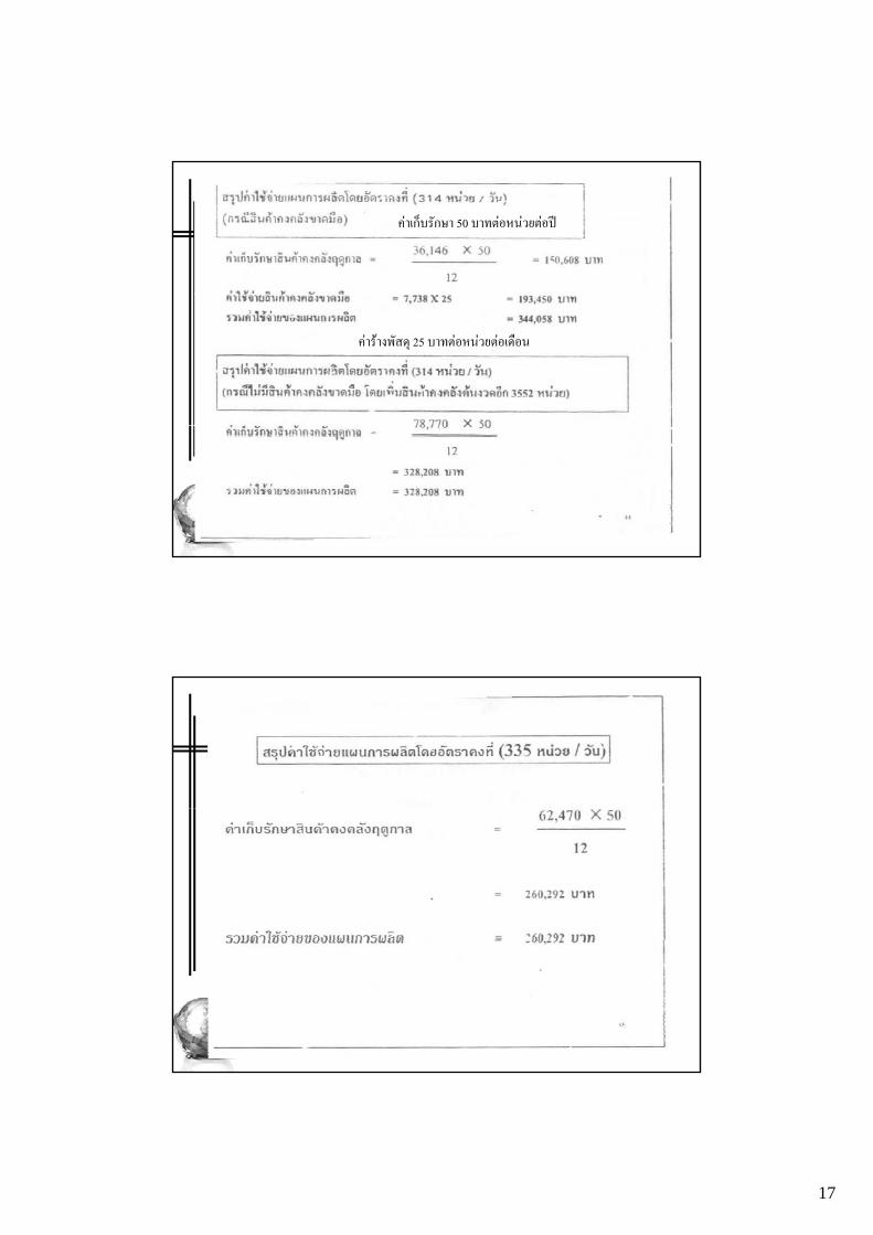
17

คาเก็บรักษา 50 บาทตอหนวยตอป

คารางพัสดุ 25 บาทตอหนวยตอเดือน

18

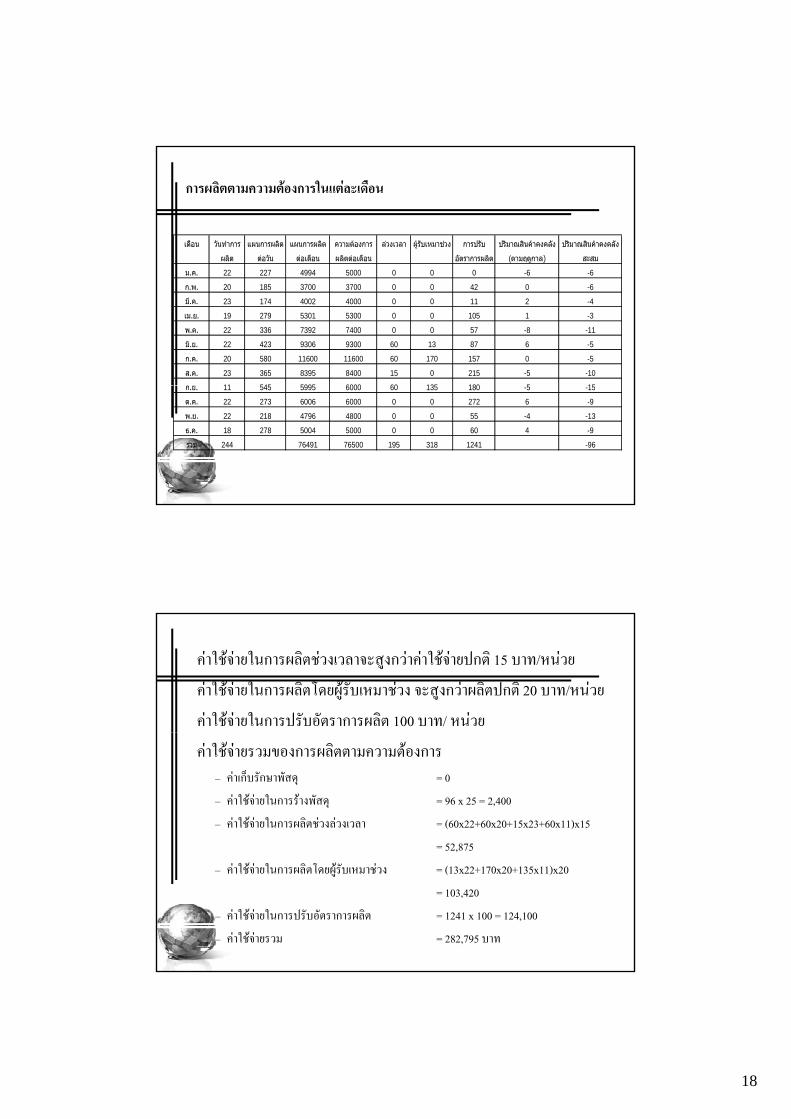
เดือน วันทําการ แผนการผลิต แผนการผลิต ความตองการ ลวงเวลา ผูรับเหมาชวง การปรับ ปริมาณสินคาคงคลัง ปริมาณสินคาคงคลัง

ผลิต ตอวัน ตอเดือน ผลิตตอเดือน อัตราการผลิต (ตามฤดูกาล) สะสม

การผลิตตามความตองการในแตละเดือน

ม.ค. 22 227 4994 5000 0 0 0 -6 -6

ก.พ. 20 185 3700 3700 0 0 42 0 -6

มี.ค. 23 174 4002 4000 0 0 11 2 -4

เม.ย. 19 279 5301 5300 0 0 105 1 -3

พ.ค. 22 336 7392 7400 0 0 57 -8 -11

มิ.ย. 22 423 9306 9300 60 13 87 6 -5

ก.ค. 20 580 11600 11600 60 170 157 0 -5

ส.ค. 23 365 8395 8400 15 0 215 -5 -10

ก ย 11 545 5995 6000 60 135 180 5 15ก.ย. 11 545 5995 6000 60 135 180 -5 -15

ต.ค. 22 273 6006 6000 0 0 272 6 -9

พ.ย. 22 218 4796 4800 0 0 55 -4 -13

ธ.ค. 18 278 5004 5000 0 0 60 4 -9

รวม 244 76491 76500 195 318 1241 -96

คาใชจายในการผลิตชวงเวลาจะสูงกวาคาใชจายปกติ 15 บาท/หนวย

คาใชจายในการผลิตโดยผูรับเหมาชวง จะสูงกวาผลิตปกติ 20 บาท/หนวย

คาใชจายในการปรับอัตราการผลิต 100 บาท/ หนวย

คาใชจายรวมของการผลิตตามความตองการ– คาเก็บรักษาพัสดุ = 0

– คาใชจายในการรางพัสดุ = 96 x 25 = 2,400

– คาใชจายในการผลิตชวงลวงเวลา = (60x22+60x20+15x23+60x11)x15

= 52,875,

– คาใชจายในการผลิตโดยผูรับเหมาชวง = (13x22+170x20+135x11)x20

= 103,420

– คาใชจายในการปรับอัตราการผลิต = 1241 x 100 = 124,100

– คาใชจายรวม = 282,795 บาท

19

70000

80000

90000

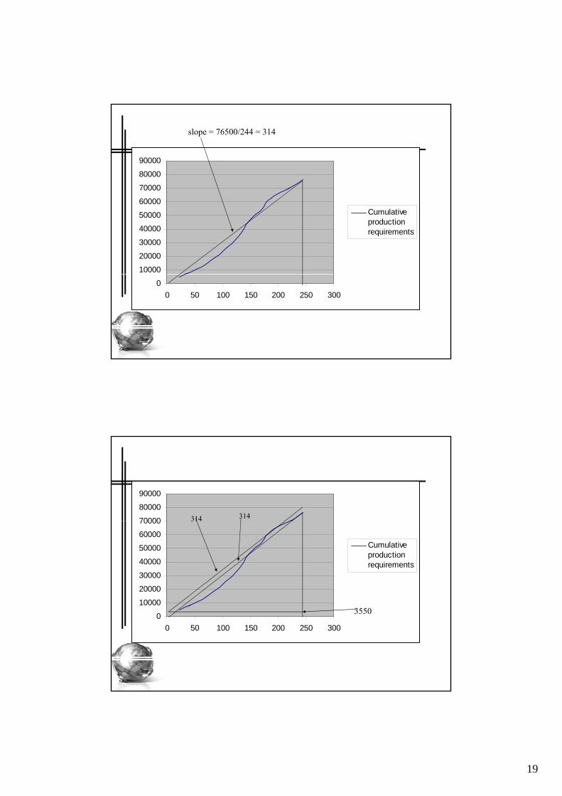
slope = 76500/244 = 314

10000

20000

30000

40000

50000

60000

70000

Cumulativeproductionrequirements

00 50 100 150 200 250 300

70000

80000

90000

314314

10000

20000

30000

40000

50000

60000

70000

Cumulativeproductionrequirements

314

00 50 100 150 200 250 300

3550

20

70000

80000

90000

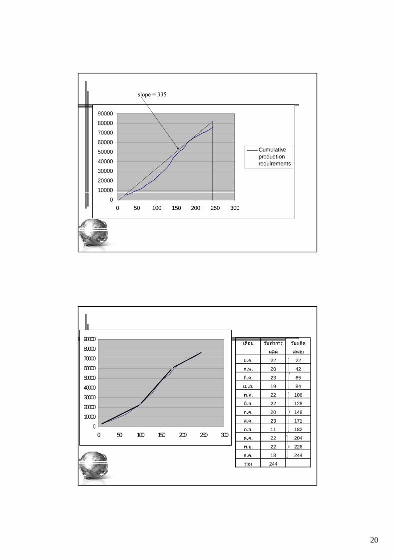
slope = 335

10000

20000

30000

40000

50000

60000

70000

Cumulativeproductionrequirements

00 50 100 150 200 250 300

70000

80000

90000เดือน วันทําการ วันผลิต

ผลิต สะสม

ม.ค. 22 22

0

10000

20000

30000

40000

50000

60000 ก.พ. 20 42

มี.ค. 23 65

เม.ย. 19 84

พ.ค. 22 106

มิ.ย. 22 128

ก.ค. 20 148

ส.ค. 23 1710

0 50 100 150 200 250 300ก.ย. 11 182

ต.ค. 22 204

พ.ย. 22 226

ธ.ค. 18 244

รวม 244

21

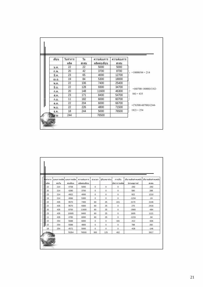
เดือน วันทําการ วัน ความตองการ ความตองการผลิต สะสม ผลิตตอเดือน สะสม

ม.ค. 22 22 5000 5000ม.ค.ก.พ. 20 42 3700 8700มี.ค. 23 65 4000 12700เม.ย. 19 84 5300 18000พ.ค. 22 106 7400 25400มิ.ย. 22 128 9300 34700ก.ค. 20 148 11600 46300ส.ค. 23 171 8400 54700ก ย 11 182 6000 60700

=18000/84 = 214

=(60700-18000)/(182-84) = 435

ก.ย. 11 182 6000 60700ต.ค. 22 204 6000 66700พ.ย. 22 226 4800 71500ธ.ค. 18 244 5000 76500รวม 244 76500

=(76500-60700)/(244-182) = 254

วันทําการ แผนการผลิต แผนการผลิต ความตองการ ลวงเวลา ผูรับเหมาชวง การปรับ ปริมาณสินคาคงคลัง ปริมาณสินคาคงคลัง

ผลิต ตอวัน ตอเดือน ผลิตตอเดือน อัตราการผลิต (ตามฤดูกาล) สะสม

22 214 4708 5000 0 0 0 -292 -292

20 214 4280 3700 0 0 0 580 288

23 214 4922 4000 0 0 0 922 1210

19 214 4066 5300 0 0 0 -1234 -24

22 435 9570 7400 60 25 221 2170 2146

22 435 9570 9300 60 25 0 270 2416

20 435 8700 11600 60 25 0 -2900 -484

23 435 10005 8400 60 25 0 1605 1121

11 435 4785 6000 60 25 0 -1215 -94

22 254 5588 6000 0 0 181 -412 -506

22 254 5588 4800 0 0 0 788 282

18 254 4572 5000 0 0 0 -428 -146

244 76354 76500 300 125 402 5917

22

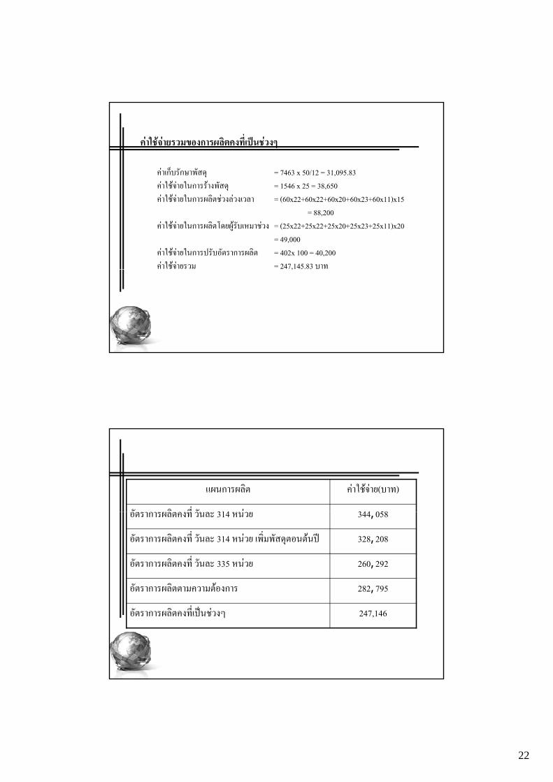
คาใชจายรวมของการผลิตคงที่เปนชวงๆ

คาเก็บรักษาพัสดุ = 7463 x 50/12 = 31,095.83คาใชจายในการรางพัสด = 1546 x 25 = 38 650คาใชจายในการรางพสดุ = 1546 x 25 = 38,650คาใชจายในการผลิตชวงลวงเวลา = (60x22+60x22+60x20+60x23+60x11)x15

= 88,200คาใชจายในการผลิตโดยผูรับเหมาชวง = (25x22+25x22+25x20+25x23+25x11)x20

= 49,000คาใชจายในการปรับอัตราการผลิต = 402x 100 = 40,200คาใชจายรวม = 247,145.83 บาท,

แผนการผลิต คาใชจาย(บาท)

ั ิ ี่ ั 314 344 058อตราการผลตคงท วนละ 314 หนวย 344,058

อัตราการผลิตคงที่ วันละ 314 หนวย เพ่ิมพัสดุตอนตนป 328,208

อัตราการผลิตคงที่ วันละ 335 หนวย 260,292

อัตราการผลิตตามความตองการ 282,795

อัตราการผลิตคงที่เปนชวงๆ 247,146

23

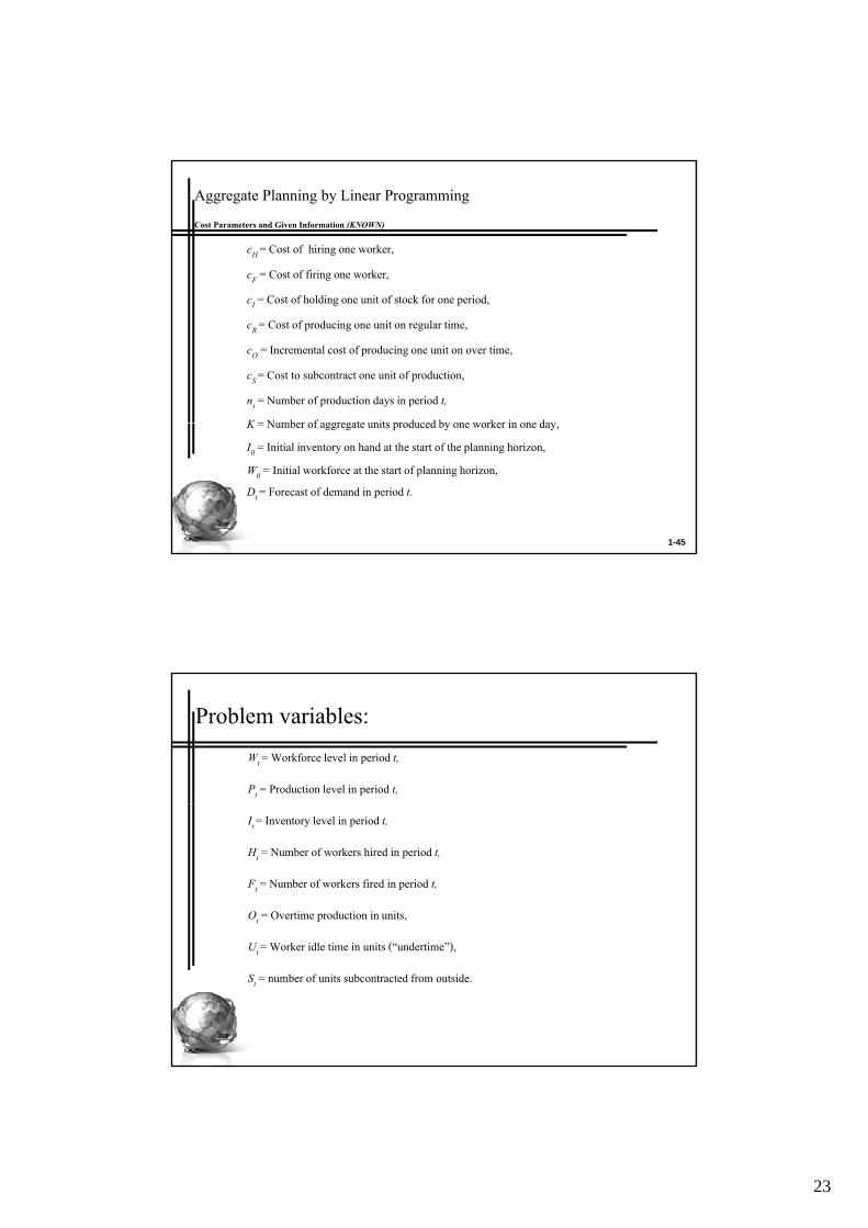
Aggregate Planning by Linear ProgrammingCost Parameters and Given Information (KNOWN)

cH = Cost of hiring one worker,

cF = Cost of firing one worker,

cI = Cost of holding one unit of stock for one period,

cR = Cost of producing one unit on regular time,

cO = Incremental cost of producing one unit on over time,

cS = Cost to subcontract one unit of production,

nt = Number of production days in period t,K = Number of aggregate units produced by one worker in one day

1-45

K = Number of aggregate units produced by one worker in one day,I0 = Initial inventory on hand at the start of the planning horizon,W0 = Initial workforce at the start of planning horizon,Dt = Forecast of demand in period t.

Problem variables:Wt = Workforce level in period t,

Pt = Production level in period t,

It = Inventory level in period t,

Ht = Number of workers hired in period t,

Ft = Number of workers fired in period t,

Ot = Overtime production in units,

Ut = Worker idle time in units (“undertime”),

St = number of units subcontracted from outside.

24

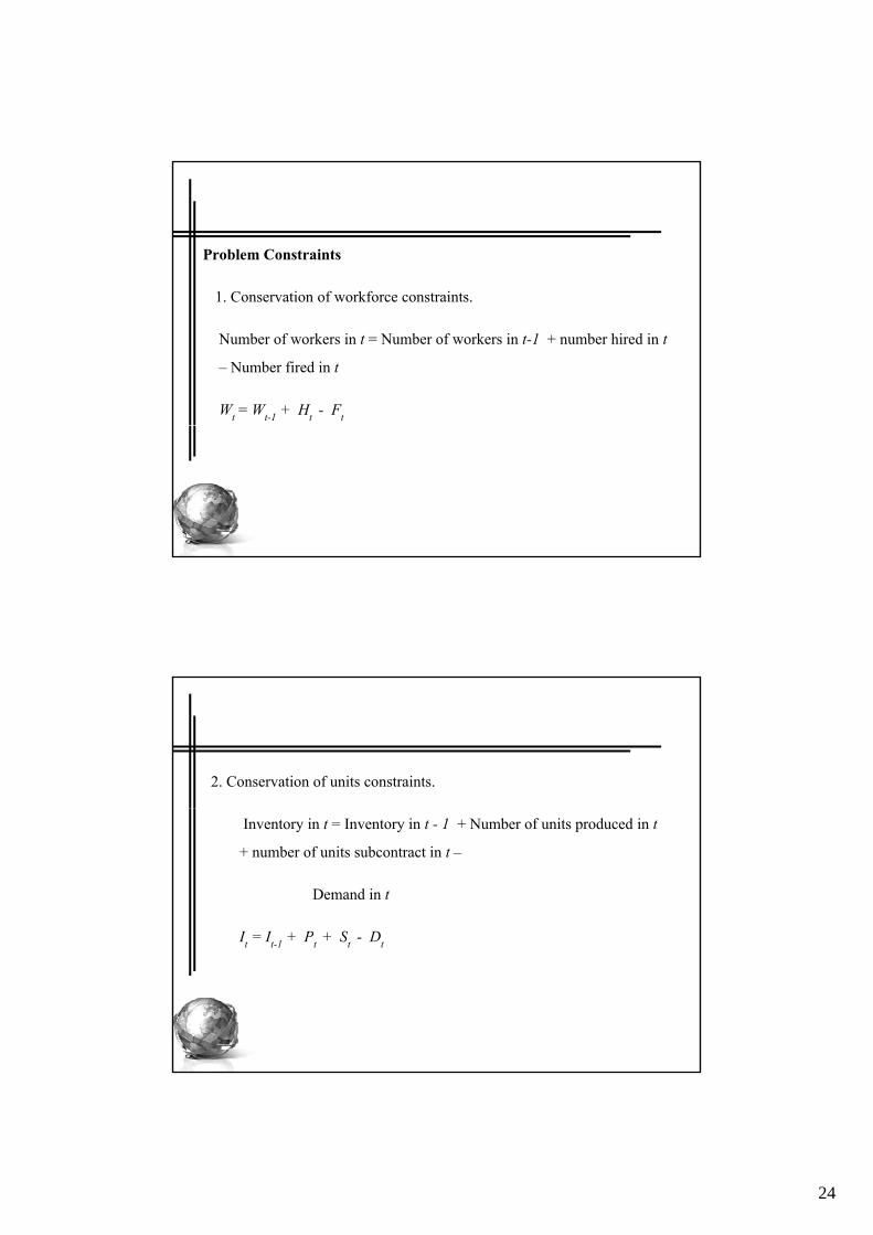
Problem Constraints

1 C ti f kf t i t1. Conservation of workforce constraints.

Number of workers in t = Number of workers in t-1 + number hired in t– Number fired in t

Wt = Wt-1 + Ht - Ft

2. Conservation of units constraints.

Inventory in t = Inventory in t - 1 + Number of units produced in t+ number of units subcontract in t –

Demand in t

I = I + P + S - DIt It-1 + Pt + St Dt

25

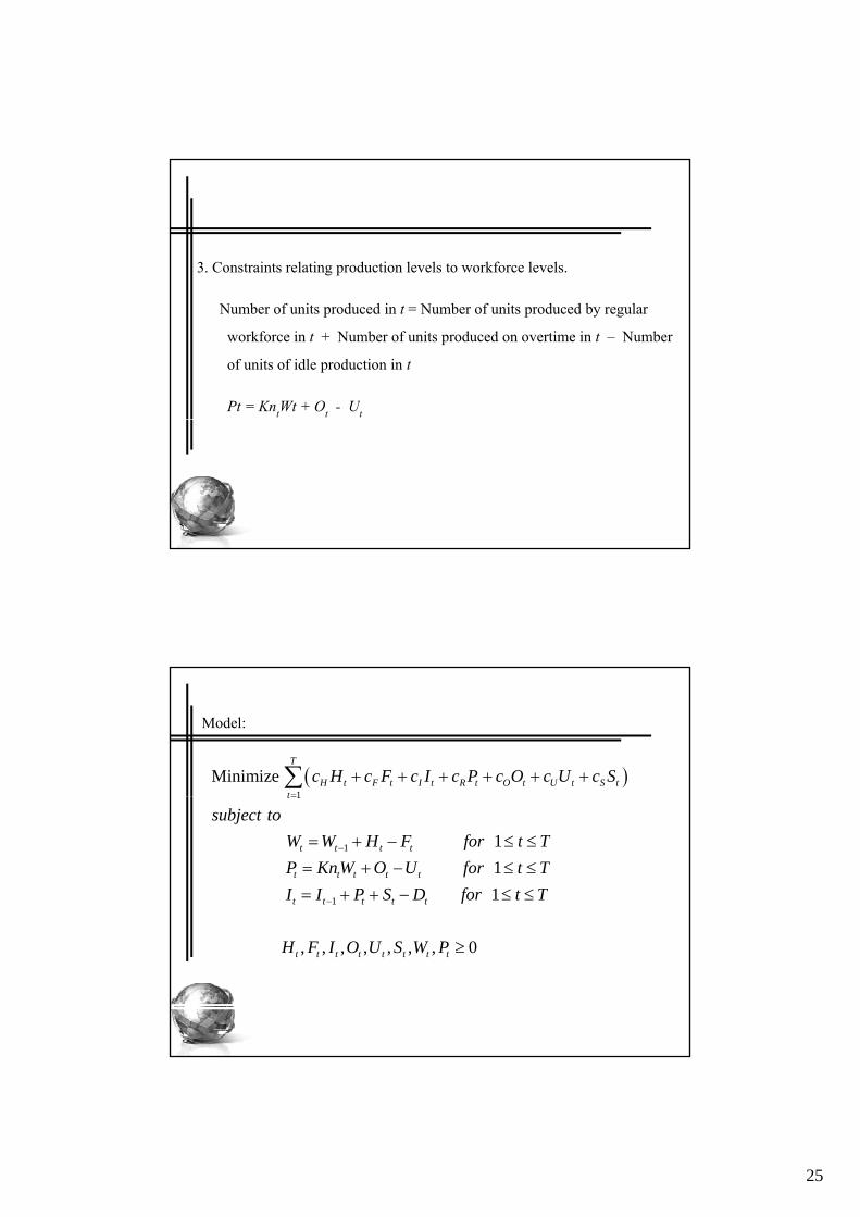
3. Constraints relating production levels to workforce levels.

Number of units produced in t = Number of units produced by regular workforce in t + Number of units produced on overtime in t – Number of units of idle production in t

Pt = KntWt + Ot - Ut

Model:

( )1

Minimize T

H t F t I t R t O t U t S tt

c H c F c I c P c O c U c S=

+ + + + + +∑1

1

1

1 1

t

t t t t

t t t t t

t t t t t

subject toW W H F for t TP KnW O U for t TI I P S D f

=

−

−

= + − ≤ ≤= + − ≤ ≤= + + − 1or t T≤ ≤

, , , , , , , 0t t t t t t t tH F I O U S W P ≥

26

Aggregate Planning in Services

• Hospitals:– Aggregate planning used to allocate funds, staff, and supplies to gg g p g pp

meet the demands of patients for their medical services

• Airlines:– Aggregate planning in this environment is complex due to the

number of factors involved– Capacity decisions must take into account the percentage of

seats to be allocated to various fare classes in order to maximize profit or yieldprofit or yield

Aggregate Planning in Services

• Restaurants:– Aggregate planning in high-volume businesses is directed gg g p g g

toward smoothing the service rate, determining workforce size, and managing demand to match a fixed capacity

– Can use inventory; however, it is perishable

27

Aggregate Planning in Services

• The resulting plan in services is a time-phased projection of service staff requirementsp j q

• Aggregate planning in manufacturing and services is similar, but there are some key differences related to:1. Demand for service can be difficult to predict2. Capacity availability can be difficult to predict3. Labor flexibility can be an advantage in services4. Services occur when they are rendered