CS 3332Probability & Statistics

(機率與統計 )

Hung-Min Sun (孫宏民 )Department of Computer Science National Tsing Hua University Email: hmsun@cs.nthu.edu.tw Office: 資電館　 640-2Phone: 校內分機 2968, 03-5742968

Empirical and Empirical and probability probability distributionsdistributionsChapter 1Chapter 1

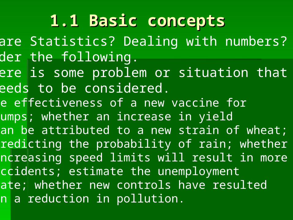
1.1 Basic concepts1.1 Basic conceptsWhat are Statistics? Dealing with numbers?Consider the following.1. There is some problem or situation that needs to be considered.Ex. The effectiveness of a new vaccine for mumps; whether an increase in yield can be attributed to a new strain of wheat; predicting the probability of rain; whether increasing speed limits will result in more accidents; estimate the unemployment rate; whether new controls have resulted in a reduction in pollution.

2. Some measures are needed to help us understand the situation better. How to create good measures?3. After the measuring instrument has been developed, we must collect data through observation. 4. Using these data, statisticians summarize the results using descriptive statistics.5. These summaries are then used to analyze the situation using statistical inferences.6. A report is presented, along with some recommendations that are based upon the data and the analysis of them.

The discipline of statistics deals with the collection & analysis data.

--- Find a pattern: among uncertainties. Filter out the noise, bound the errors, derive

the confidence.

---- Think carefully: about the investigations

& problems. Make sense out of the observations, pick the

proper math models.

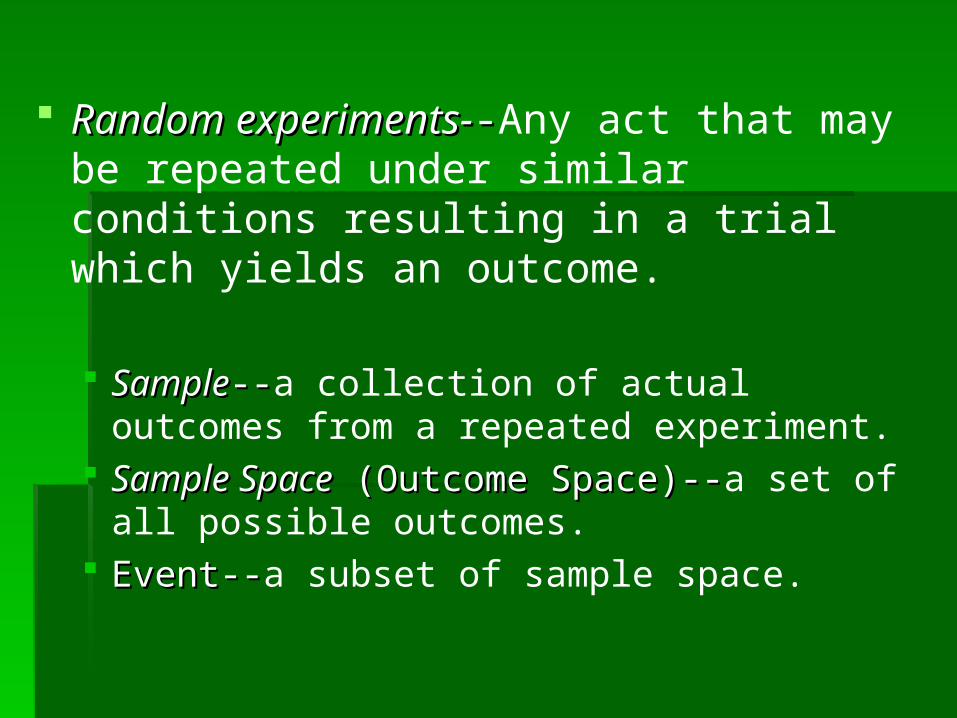
Random experiments-Random experiments---Any act that may be repeated under similar conditions resulting in a trial which yields an outcome.

SampleSample----a collection of actual outcomes from a repeated experiment.

Sample SpaceSample Space (Outcome Space)-- (Outcome Space)--a set of all possible outcomes.

Event--Event--a subset of sample space.

Two dice are cast and the total number of spots on the sides that are ”up” are counted. The sample space is S = {2, 3, 4, . . . , 12}

Toss a fair coin. The sample space is S = {H, T} .

A fair coin is flipped successively at random until heads is observed on two successive flips. If we let y denote the number of flips of the coin that are required, then S = {y : y = 2, 3, . . . .} .

Given a random experiment with sample space S , a function X mapping each element of S to a unique real number is called a random variablerandom variable .

For each element s from the sample space S , denote this function by X(s) = x and call the range of X or the space of X : R = {x : X(s) = x, for some s in S}

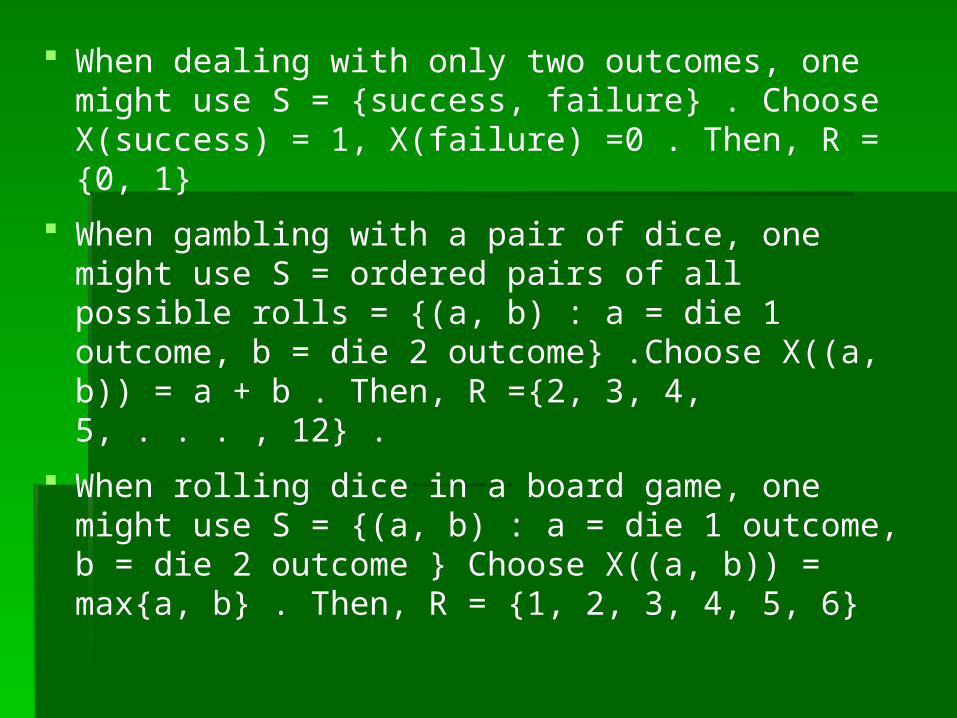
When dealing with only two outcomes, one might use S = {success, failure} . Choose X(success) = 1, X(failure) =0 . Then, R = {0, 1}

When gambling with a pair of dice, one might use S = ordered pairs of all possible rolls = {(a, b) : a = die 1 outcome, b = die 2 outcome} .Choose X((a, b)) = a + b . Then, R ={2, 3, 4, 5, . . . , 12} .

When rolling dice in a board game, one might use S = {(a, b) : a = die 1 outcome, b = die 2 outcome } Choose X((a, b)) = max{a, b} . Then, R = {1, 2, 3, 4, 5, 6}

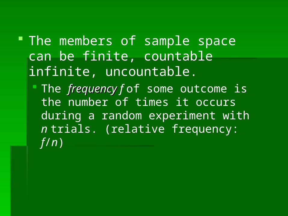
The members of sample space can be finite, countable infinite, uncountable. The frequency frequency f of some outcome is the

number of times it occurs during a random experiment with n trials. (relative frequency: f/n)

Density (Relative Frequency) Histogram The density histogram, say h(x), graphically

reports the relative freq. of each possible outcome x0. For small n, f/n is very unstable. As n increases,h(x0) = f0/n →p0= f(x0).

h(x) will approach the probability mass function(p.m.f.) f(x). Density histogram Probability histogram.⇒

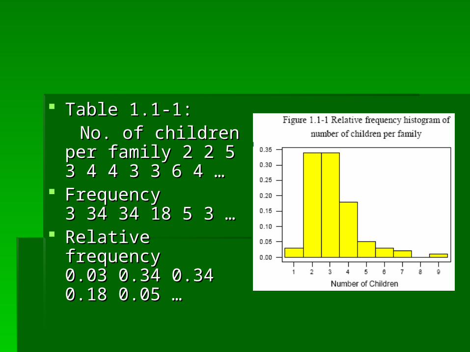
Table 1.1-1: Table 1.1-1: No. of children per No. of children per

family 2 2 5 3 4 4 3 3 family 2 2 5 3 4 4 3 3 6 4 …6 4 …

FrequencyFrequency3 34 34 18 5 3 …3 34 34 18 5 3 …

Relative frequencyRelative frequency0.03 0.34 0.34 0.18 0.03 0.34 0.34 0.18 0.05 …0.05 …

1.2 The mean, variance, 1.2 The mean, variance, and standard deviationand standard deviation

” measures of ”center” mean

” measures of ”spread” variance

Mean: (1) Statistical measure of location (2) Mathematical expectation of a

corresponding random variable (3) The first moment about the region of a mass

function f(x)

)()(

)()()()( 22_

11

yprobabilitvalue

xfxxfxxfxxxf kkxall

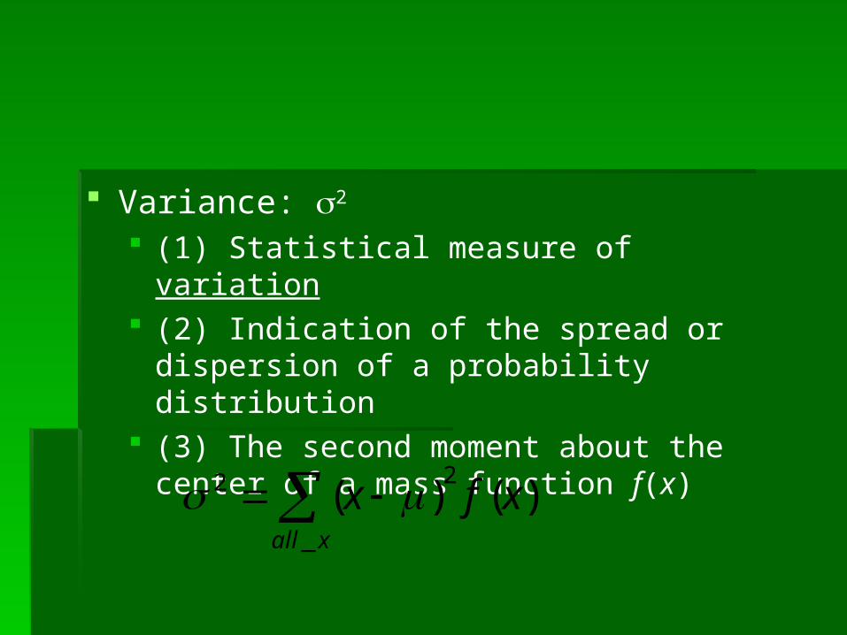
Variance: 2

(1) Statistical measure of variation (2) Indication of the spread or dispersion of a

probability distribution (3) The second moment about the center of a

mass function f(x)

)()(2

_

2 xfxxall

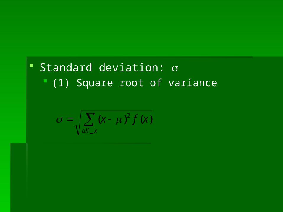
Standard deviation: (1) Square root of variance

xall

xfx_

2 )()(

x {1, 2, 3} and the p.m.f. is given by f(1) = 3/6, f(2) =2/6, f(3) = 1/6 . Weighted mean (weighted average) is

1 · 3/6 + 2 · 2/6+ 3 · 1/6= 10/6

=10/6

2=(1-10/6)2×3/6+(2-10/6)2×2/6+(3-10/6)2×1/6=120/216

= (2)1/2=(120/216)1/2=0.745

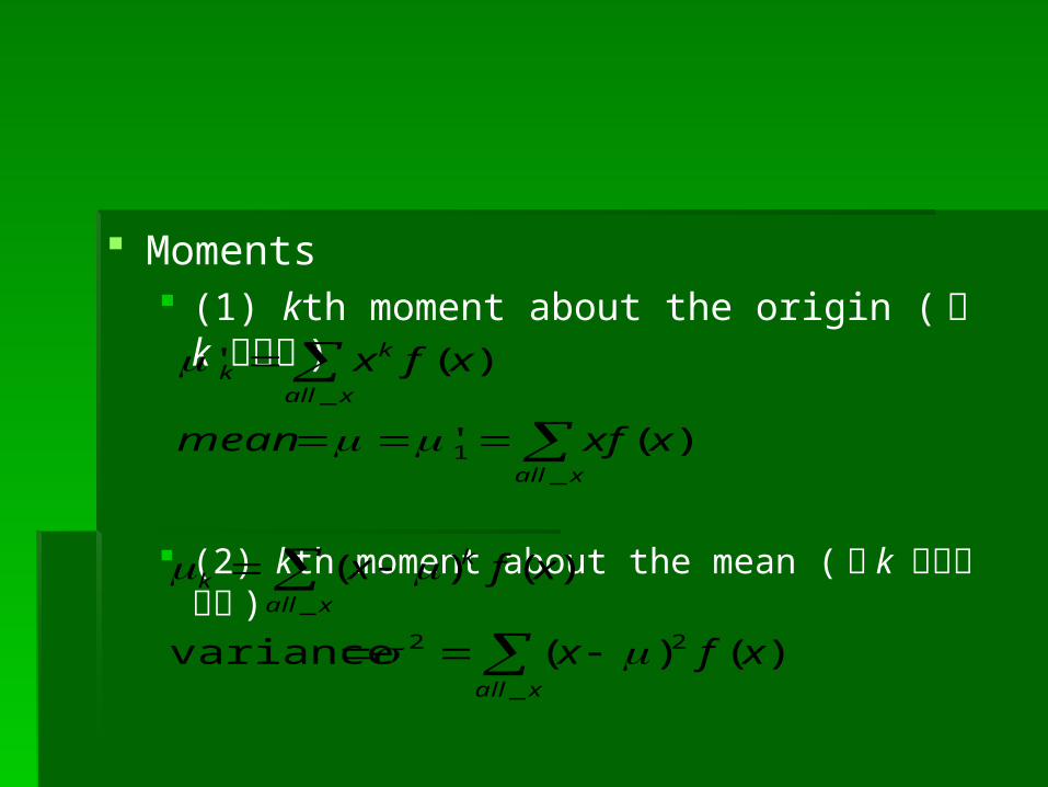
Moments (1) kth moment about the origin ( 第 k 級動差 )

(2) kth moment about the mean ( 第 k 級中央動差 )

xall

xall

kk

xxfmean

xfx

_1

_

)('

)('

xall

xall

kk

xfx

xfx

_

22

_

)()(variance

)()(

1.3 Continuous-type data1.3 Continuous-type data Group the data into classes

1.1. MaximumMaximum ，， MinimumMinimum ，， RangeRange

2. Select the number of classes ， k=5 to 20

3. Each interval begins and ends halfway between two possible values.

4. The 1st interval begin about as much below the smallest value as the last interval ends above the largest.

5. The intervals are called class intervalsclass intervals and the boundaries are classes boundariesclasses boundaries or cutpointscutpoints.. (c0, c1), (c1, c2), …, (ck-1, ck): k class intervals.

6. The class limitsclass limits are the smallest and largest possible observed values in a class.

7. The class markclass mark ui is the midpoint of Class i.

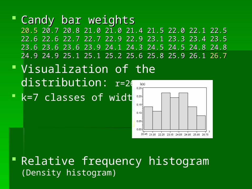
Candy bar weightsCandy bar weights20.520.5 20.7 20.8 21.0 21.0 21.4 21.5 22.0 22.1 22.5 20.7 20.8 21.0 21.0 21.4 21.5 22.0 22.1 22.522.6 22.6 22.7 22.7 22.9 22.9 23.1 23.3 23.4 23.522.6 22.6 22.7 22.7 22.9 22.9 23.1 23.3 23.4 23.523.6 23.6 23.6 23.9 24.1 24.3 24.5 24.5 24.8 24.823.6 23.6 23.6 23.9 24.1 24.3 24.5 24.5 24.8 24.824.9 24.9 25.1 25.1 25.2 25.6 25.8 25.9 26.1 24.9 24.9 25.1 25.1 25.2 25.6 25.8 25.9 26.1 26.726.7

Visualization of the distribution: r=26.7-20.5=6.2

k=7 classes of width 0.9

Relative frequency histogram (Density histogram)

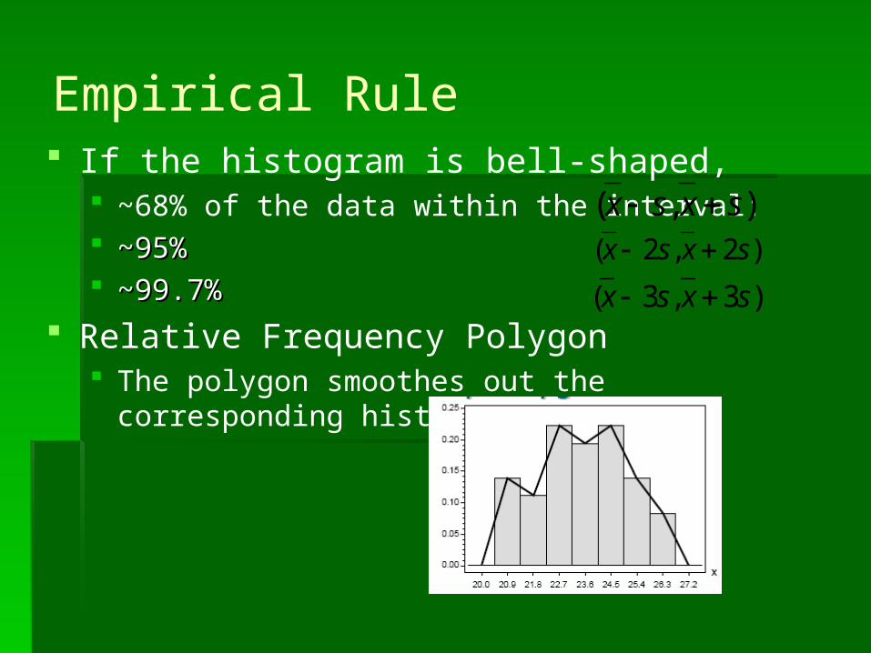
Empirical Rule If the histogram is bell-shaped,

~68% of the data within the interval: ~95%~95% ~99.7%~99.7%

Relative Frequency Polygon The polygon smoothes out the corresponding

histogram somewhat.

),( sxsx )2,2( sxsx

)3,3( sxsx

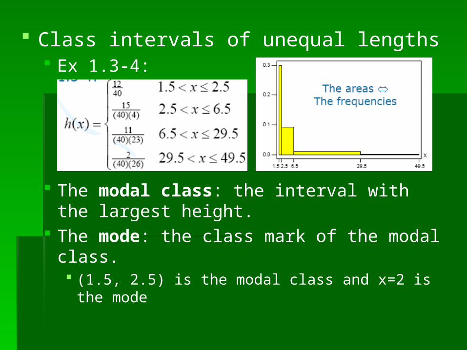
Class intervals of unequal lengths Ex 1.3-4:

The modal class: the interval with the largest height.

The mode: the class mark of the modal class. (1.5, 2.5) is the modal class and x=2 is the mode