data analysis and probability calculations using a ti …albert/dap/calculator_help.pdfdata analysis...

Data Analysis and Probability Calculations using a TI 83-Plus/TI 84-Plus calculator

March 2007

TABLE OF CONTENTS DATA ANALYSIS 1. Single batch of measurement data

• Entering your data into the calculator • Graphing your data • Summarizing your data

2. Categorical data 3. Comparing batches of measurement data

• Entering your data into the calculator • Graphing the data • Getting summaries

4. Relationships

• Entering the data • Graphing the data • Computing summary statistics (least-squares line) • Computing residuals • Computing correlation • Median-median line

PROBABILITY 5. Counting Formulas

• Number of arrangements (permutations) • Number of combinations

6. Basic Simulation Commands Random commands built into the calculator

• Random numbers • Random integers • Random normals • Random binomials

Other simulation talks available by several key strokes

• Randomly permute a list

• Take a random sample without replacement • Take a random sample with replacement

7. Programming a Probability Simulation

• Simulating a lottery game

8. Summarizing a Probability Distribution 9. Binomial and Normal Calculations

• Finding binomial probabilities and cumulative probabilities • Normal calculations (density values, probabilities, percentiles)

10. Integration 11. Transferring Data between Calculators

1. SINGLE BATCH OF MEASUREMENT DATA As an example, we consider the high school completion rates of all states and the District of Columbia described in Topic D2. Entering your data into the calculator: First we have to enter these data into the calculator. 1. Push key strokes Stat -> Edit -> 1. Edit You will see lists L1, L2, … along the top.

We will enter the data into list L1. We move the cursor to the space below L1. Then we type in the data values, one by one, each time hitting the Enter key to place the data value into the list. Graphing your data: To set up graphing these data, you first push 2nd STAT PLOT This will bring up a set of options for constructing various types of plots.

Suppose we wish to make our graph Plot 1. Then we select Plot 1 and see the following screen.

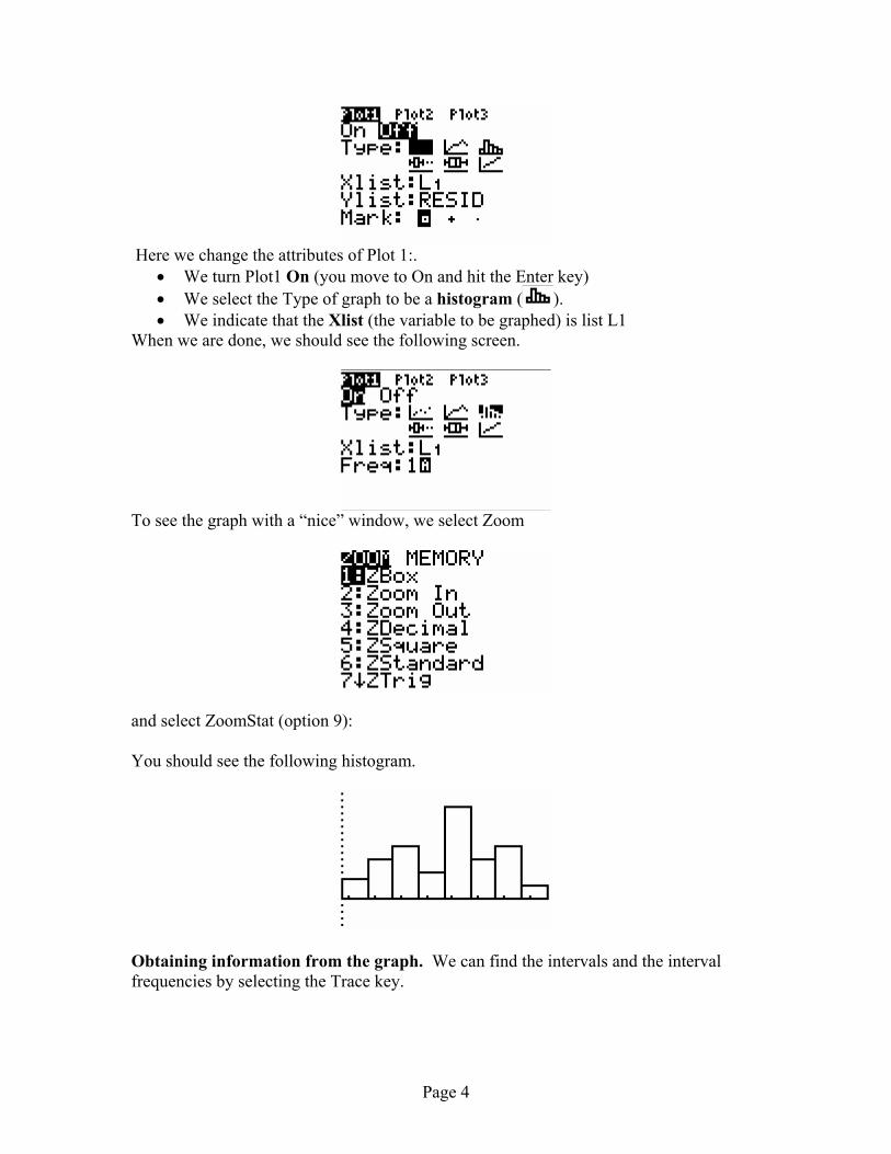
Here we change the attributes of Plot 1:.

• We turn Plot1 On (you move to On and hit the Enter key) • We select the Type of graph to be a histogram ( ). • We indicate that the Xlist (the variable to be graphed) is list L1

When we are done, we should see the following screen.

To see the graph with a “nice” window, we select Zoom

and select ZoomStat (option 9): You should see the following histogram.

Obtaining information from the graph. We can find the intervals and the interval frequencies by selecting the Trace key.

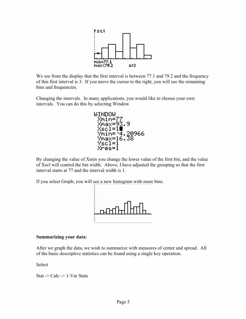
We see from the display that the first interval is between 77.1 and 79.2 and the frequency of this first interval is 3. If you move the cursor to the right, you will see the remaining bins and frequencies. Changing the intervals. In many applications, you would like to choose your own intervals. You can do this by selecting Window

By changing the value of Xmin you change the lower value of the first bin, and the value of Xscl will control the bin width. Above, I have adjusted the grouping so that the first interval starts at 77 and the interval width is 1. If you select Graph, you will see a new histogram with more bins.

Summarizing your data: After we graph the data, we wish to summarize with measures of center and spread. All of the basic descriptive statistics can be found using a single key operation. Select Stat -> Calc -> 1-Var Stats

You will see the 1-Var Stats command in your main window. You add list L1, since we wish to summarize L1.

We get the following display (note that you will see only about half of the statistics in the window – you scroll down with the arrow key to get the remaining statistics).

Most of these statistics should be self-explanatory. Sx is the usual standard deviation. Xσ is defined similarly to Sx, but one divides the sum of squared deviations by the

sample size n (instead of n-1). Q1, Med, Q3 are respectively the lower quartile, the median, and the upper quartile. 2. CATEGORICAL DATA Although the calculator is not easy to use directly with data that are categorical, it is possible to recode the data and use the histogram capabilities to tally these data. Suppose we roll a die 100 times – we are interested in the frequencies of the categorical outcomes

“one”, “two”, “three”, “four”, “five”, “six” On the calculator, we represent these outcomes by the numbers 1, 2, 3, 4, 5, 6. By use of the randInt command, we can simulate die rolls by choosing 100 random integers between 1 and 6. In the output below, we store these 100 random integers in the list L1.

To tally these data, we first set up Plot1 to be a histogram of the list L1:

When we choose ZOOM -> ZoomStat, we get the unusual looking histogram

When we are interested in tallying data, we’d like some control about how the intervals in the histogram are constructed. By selecting the WINDOW option, we indicate that the first interval will start at 1 (the smallest die rolls), and then the interval width is 1. (On the calculator, the left-endpoint is included in the interval and the right-endpoint is not.)

When we select GRAPH, we see a better-looking histogram.

We can find the frequencies of the intervals by use of the TRACE key.

By tracing over the histogram, we see that the frequencies of the six die rolls are Die Roll 1 2 3 4 5 6 Frequency 17 18 17 19 13 16 Also it is possible to find these frequencies by the sum command. For example, the number of die rolls equal to 1 is given by

The number of die rolls less than or equal to 4 is given by

3. COMPARING BATCHES OF MEASUREMENT DATA Here we compare the high school completion rates of the Midwest States and the Southeast States discussed in Topic D4. Entering your data into the calculator: To begin, we enter the completion rates of the Midwest States in list L1 and the completion rates of the Southeast States in list L2.

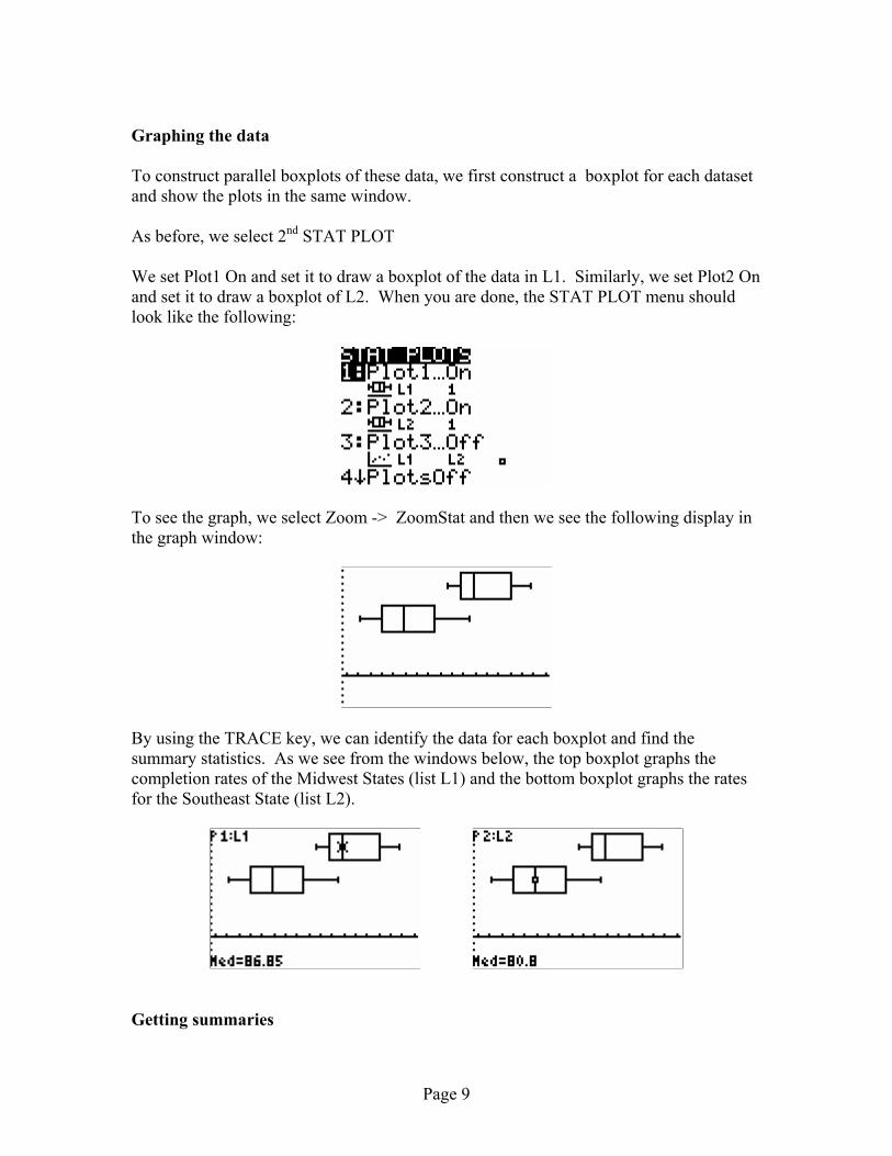
Graphing the data To construct parallel boxplots of these data, we first construct a boxplot for each dataset and show the plots in the same window. As before, we select 2nd STAT PLOT We set Plot1 On and set it to draw a boxplot of the data in L1. Similarly, we set Plot2 On and set it to draw a boxplot of L2. When you are done, the STAT PLOT menu should look like the following:

To see the graph, we select Zoom -> ZoomStat and then we see the following display in the graph window:

By using the TRACE key, we can identify the data for each boxplot and find the summary statistics. As we see from the windows below, the top boxplot graphs the completion rates of the Midwest States (list L1) and the bottom boxplot graphs the rates for the Southeast State (list L2).

Getting summaries

To get summary statistics, we apply the Stat -> Calc -> 1-Var Stats command twice, one time on list L1 and one time on L2.

4. RELATIONSHIPS Here we look at the weather data from topic D5, where the January temperature and the July temperature were collected for 10 cities. Entering the data We put the January temperatures in a list JAN and the July temperatures in list JULY.

Graphing the data To construct a scatterplot, we select 2nd STAT PLOT. We change attributes of Plot 1. We turn this plot ON, choose a scatterplot as the TYPE, and indicate that JAN, JULY are the Xlist, Ylist variables.

To display this graph, we select ZOOM -> ZoomStat

Computing summary statistics To compute some basic statistics, we select STAT -> Calc -> 2-Var Stats, and then type in the names of the two variables, separated by a comma.

This command gives basic statistics for JAN, for JULY and also gives the sum of (JAN x JULY):

To fit a least-squares line, we choose STAT -> Calc -> LinReg(ax+b). As above, we follow this command with the x-variable (JAN) and the y-variable (JULY).

We get the following output:

Suppose we wish to plot this least-squares line, we use the same command as above, with the exception that we indicate that the least-squares line function is stored in Y1.

To show this line equation on the graph, we first select Y= and select Y1 by moving to the “=” sign and pushing Enter.

Now when we select Graph, we see the scatterplot and least-squares line drawn on top.

Compute residuals To have the calculator find the residuals, we assume that we have already fit a least-squares line. There is a variable created called RESID – we have to rename a list to this variable name and we’ll see the residuals. Select STAT -> Edit -> Edit Go to the first clear list heading and name this list RESID. (When you move to the list heading, select 2nd INS, and type RESID as the list name.) You should see the residuals in the list RESID:

Compute correlation To compute the correlation, we first select the command DiagnosticOn Next, you select the linear regression command STAT -> Calc -> LinReg(ax+b). Enter the x and y variables and you will see the value of the correlation below the coefficients of the least-squares line.

Median-median line

One fits a median-median line much like the least-squares line. We choose STAT -> Calc -> Med-Med , and then enter the names of the x and y variables:

We see the following output:

5. COUNTING FORMULAS Number of arrangements (permutations) nPr – number of arrangement of r of n objects

(MATH PROB 2) Example : Say you own ten books and you are interested in the number of ways of arranging five of the books in the shelf. Here n = 10 and r = 5. The number of ways is ! – number of permutations of n objects

(MATH PROB 4) Example. Suppose you wish to arrange ten books on the shelf. The number of ways is

Number of combinations nCr – number of combinations of n objects, taken r at a time

(MATH PROB 3) Example. Suppose you wish to select five people from a room of nine to work on a service project. Here n = 9 and r = 5 and the number of combinations is

6. BASIC SIMULATION COMMANDS RANDOM COMMANDS BUILT INTO THE CALCULATOR Random numbers rand[number of trials] – generates a sequence of random numbers between 0 and 1

(MATH PROB 1) Example: Suppose I wish to generate 8 random numbers and store them in list L1.

We can see the random numbers in the table view.

Random integers randInt(lower, upper[, number of trials]) – generates a sequence of random integers between lower and upper, inclusive

(MATH PROB 5) Example: Suppose I wish to simulate 5 random dice rolls (each roll is equally likely to be 1, 2, 3, 4, 5, 6).

Random normals

randNorm(mean, stand dev[, number of trials]) – generates a sequence of normally distributed random numbers with a give mean and standard deviation.

(MATH PROB 6) Example: Suppose I wish to simulate 4 numbers from a normal distribution with mean 100 and standard deviation 10.

Random binomials randBin(number of trials, probability of success[, number of simulations) – generates a sequence of binomial random variables with given values of n (number of trials ) and p (probability of success)

(MATH PROB 7) Example: Consider the simple coin-tossing experiment of tossing ten coins and counting X, the number of heads. (Here n = 10 and p = .5.) I wish to simulate this experiment five times, obtaining five values of X:

OTHER SIMULATION TASKS AVAILABLE BY SEVERAL KEY STROKES Randomly permute a list Example: Suppose we wish to permute the elements of L1. We assume that L1 has 10 elements. (Make the appropriate changes if the number of elements is a different number.) 1. rand(10) -> L2 this command puts 10 random numbers in list L2 2. SortA(L2, L1) this command sorts the values in L2, bringing along L1 List L1 will contain the randomly arranged list. Take a random sample without replacement Example: Suppose you again have a list L1 containing 10 elements and we are interested in taking a sample of 5 without replacement.

1. rand(10) -> L2 this command puts 10 random numbers in list L2 2. SortA(L2, L1) this command sorts the values in L2, bringing along L1 The first 5 elements in L1 are your sample. Take a random sample with replacement Example: Suppose you again have a list L1 containing 10 elements and we are interested in taking a sample of 5 with replacement. L1(randInt(1,10)) this command simulates a random integer between 1 and 10

and displays the corresponding value of list L1 Repeat the command L1(randInt(1,10)) until you’ve taken a sample of size k 7. PROGRAMMING A PROBABILITY SIMULATION Writing a simple “Set Up” program. Writing a program to simulate the Lottery example. Running the simulation and summarizing the results. --------------------------------------------------------------------------------------- Writing a simple “Set Up” program. First we write a simple program that will clear the list L3 and set a counter I to 0.

1. Press PRGM to display the PRGM NEW menu. 2. Press ENTER to select 1: Create New. The Name = prompt is displayed with alpha-lock on. Press [S] [E] [T] [S] [I] [M], and then press ENTER to name this program SETSIM. You are now in the Program Editor. The colon (:) in the first column indicates the beginning of the first line in the program.

3. Press STAT 4 to select 4: ClrList . Then press 2nd [L3]. You should see the command ClrList L3 (this command clears list L3)

Press ENTER to go to the next line. 4. Press 0, then STO>, then ALPHA [I]. You should see 0→ I (this command stores the value 0 in the variable I) Press ENTER, and then 2nd QUIT to leave the programming environment. 5. To run this program, press PRGM to display the PRGM EXEC menu. Press the cursor to move down through the list of programs until you select SETSIM and press ENTER. You’ll see prgmSETSIM on your home screen. Press ENTER to run this program. Now list L3 will be cleared and the variable I will be set to 0 (you can check this if you want.) Writing a program to simulate the Lottery example. Let’s simulate the lottery game described in Topic P4. We have selected the three-digit number 123. A winning number is chosen from all possible three-digit numbers from 000 to 999. We are interested in the probability that “123” will match the winning number in exactly 1 digit, in exactly 2 digits, and in exactly 3 digits. Here is the simulation experiment that we wish to program. Step 1. We simulate one random three-digit number between 000 and 999. Step 2. We record the number of digits that this random number has in common with our number 123. (If the random number is 324, there is exactly one digit in common, and if the random number is 163, there are exactly two digits in common. Note that place value of the digits is important, so the number of matches of the random number “312” with “123” is zero.) Step 3. We store the number of matching digits. We wish to repeat this experiment many times, so we can get a reasonable estimate at the probability that the random number matches our number in 1 digit, in 2 digits, and in 3 digits.

We create a new program called LOTTERY that will do one simulation experiment. We assume that the program SETSIM has already been run, so list L3 is clear and the counter I has been set to 0.

1. As before, press PRGM to display the PRGM NEW menu. 2. Press ENTER to select 1: Create New. Press [L] [O] [T] [T] [E] [R] [Y], and then press ENTER to name this program LOTTERY. Now you can type in the program – in the left column I indicate the key strokes, in the middle column , I show what appears on the screen, and in the right column, I explain what this command accomplishes. What you type What you see on the screen What it does 2nd [{] 1, 2, 3 2nd [}] STO> 2nd [L1]

{1, 2, 3}→ L1 This creates a list with elements 1, 2, 3 and stores the list in L1

MATH PROB 5 (0, 9, 3) STO> 2nd [L2]

RandInt(0,9,3) → L2 This generates three random digits between 0 and 9 and places the digits in list L2

ALPHA [I] +1 STO> ALPHA[I]

I+1 → I Updates the counter I by one.

2nd [LIST] MATH 5 2nd [L1] 2nd [TEST] 1 2nd [L2]) STO> 2nd [L3]( ALPHA [I])

Sum(L1=L2) → L3 (I) Counts the number of matches between the random number and 123 and stores the result in list L3.

Here is the how the program actually looks on the screen when I am finished.

When you have entered these four commands, press 2nd QUIT to leave the programming environment. Running the simulation and summarizing the results. We’ve done the hard work – now we can simulate this lottery experiment.

1. In the home screen, press PRGM to display the PRGM EXEC menu, select SETSIM and press ENTER. You’ll see prgmSETSIM This will clear list L3 and set the counter I to zero. 2. Now press PRGM, select LOTTERY and press ENTER. You will see prgmLOTTERY When you press ENTER, this lottery experiment is run once and the number of matches is displayed. 3. To repeat this simulation multiple times, just press ENTER multiple times – you will see the number of matches for the experiments and the results are being stored in list L3. 4. At some point (say after a minute of repeatedly pressing ENTER), you will want to summarize the results. A simple way to do this is to

construct a histogram of the data in L3 trace over the histogram to see the counts of the different outcomes

In my experiment, here is my histogram of the outcomes:

I trace over the histogram, and get the following displayed frequencies:

I place these counts in a table.

Outcome (number of matches) Count 0 71 1 16

2 3 TOTAL 90

I convert the observed counts to probabilities by dividing the counts of the different outcomes by 90.

Outcome (number of matches) Probability 0 71/90 = .79 1 16/90 = .18 2 3/90 = .03

TOTAL 1 8. SUMMARIZING A PROBABILITY DISTRIBUTION Suppose you have a die with one side showing 1, two sides showing 2, and three sides showing 3. If X is the number observed on a single roll, then X has the following probability distribution.

X Prob(X) 1 1/6 2 2/6 3 3/6

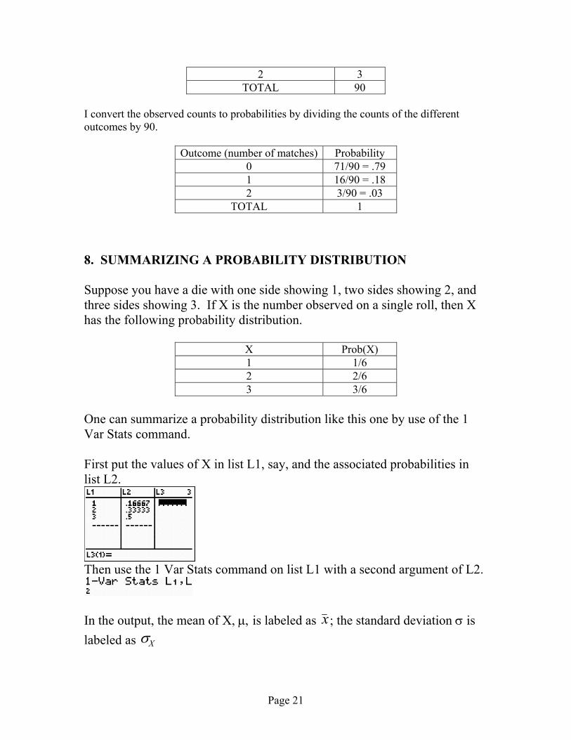
One can summarize a probability distribution like this one by use of the 1 Var Stats command. First put the values of X in list L1, say, and the associated probabilities in list L2.

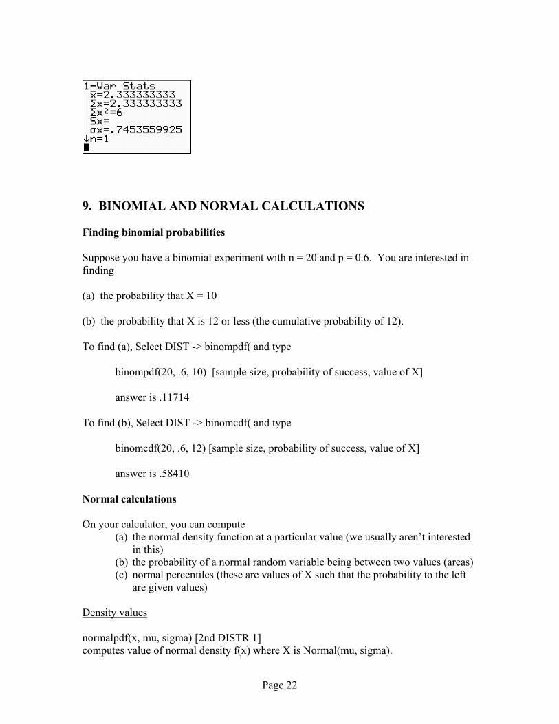
Then use the 1 Var Stats command on list L1 with a second argument of L2.

In the output, the mean of X, µ, is labeled as x ; the standard deviation σ is labeled as Xσ

9. BINOMIAL AND NORMAL CALCULATIONS

Finding binomial probabilities

Suppose you have a binomial experiment with n = 20 and p = 0.6. You are interested in finding

(a) the probability that X = 10

(b) the probability that X is 12 or less (the cumulative probability of 12).

To find (a), Select DIST -> binompdf( and type

binompdf(20, .6, 10) [sample size, probability of success, value of X]

answer is .11714

To find (b), Select DIST -> binomcdf( and type

binomcdf(20, .6, 12) [sample size, probability of success, value of X]

answer is .58410

Normal calculations On your calculator, you can compute

(a) the normal density function at a particular value (we usually aren’t interested in this)

(b) the probability of a normal random variable being between two values (areas) (c) normal percentiles (these are values of X such that the probability to the left

are given values) Density values normalpdf(x, mu, sigma) [2nd DISTR 1] computes value of normal density f(x) where X is Normal(mu, sigma).

Example: To find value of standard normal density at x =-1, normalpdf(-1, 0, 1) = .241970745 Normal probabilities (areas) normalcdf(a, b, mu, sigma) [2nd DIST 2] computes probability P(a < X < b) where X is Normal(mu, sigma). Example: If height X is normal(64, 4), the probability a student’s height is between 60 and 70 is normalcdf(60, 70, 64, 4) = .7745375117 (By the way, if you wish to put - ∞ or + ∞ , use -1E99 and 1E99, respectively.) In the above story, if you wish to compute P(X ≤ 62), use normalcdf(-1E99, 62, 64, 4) = .3085375322. Normal percentiles invnorm(p,mu,sigma) [2nd DIST 3] finds pth percentile (p a value between 0 and 1) of X where X is Normal(mu, sigma). Example: If height X is normal(64, 4), and we want to find the 25th percentile of distribution, use invnorm(.25,64, 4) = 61.302041 9. INTEGRATION Here are some basic steps for integrating a function between two values. 1. Define the function as Y4, say. 2. Plot the function. 3. Use integration function fnInt(Y4, X 0, 100). 4. Adjust definition of Y4 (if necessary) to make sure it is a density function. 5. Use integration function to find probabilities. 6. Write a simple program to compute F(X) for a user inputted X: Prompt Y Disp “CUM PROB:”

fnInt(Y4,X,0,Y) 7. Use this program to find any percentile of X. 8. Can use the integration function to find the mean and standard deviation of X. 10. TRANSFERRING DATA AND PROGRAMS BETWEEN CALCULATORS: Between a TI-84 Plus and a TI-84 Plus

LEFT RIGHT (Sending) (Receiving) I’m assuming that you want to send information from the LEFT calculator to the RIGHT calculator. 1. Attach the USB cable from the top right edge of the LEFT calculator to the top right edge of the RIGHT calculator. 2. On both calculators, press 2nd LINK. 3. You’ll see the following screen:

4. Suppose you wish to send one or more Lists from the LEFT to the RIGHT calculator: (a) Select menu item 4 on the LEFT calculator. (b) Press the up and down arrow keys until you find a list you wish to send.

(c) Press ENTER to select or deselect a list. Selected items are marked with a square box. You can send more than one list by selecting multiple lists. (d) On the RIGHT calculator, go to the menu item RECEIVE and press ENTER. (e) To send the lists, press the right arrow on the LEFT calculator to display the TRANSMIT menu and select 1: TRANSMIT. (f) After all lists have been transferred, you should see the message DONE on both calculators. 5. Suppose you wish to send one or more Programs from the LEFT to the RIGHT calculator: (a) Select menu item 3 on the LEFT calculator. (b) Press the up and down arrow keys until you find a program you wish to send. (c) Press ENTER to select or deselect a program. Selected items are marked with a square box. You can send more than one program by selecting multiple programs. (d) On the RIGHT calculator, go to the menu item RECEIVE and press ENTER. (e) To send the lists, press the right arrow on the LEFT calculator to display the TRANSMIT menu and select 1: TRANSMIT. (f) After all programs have been transferred, you should see the message DONE on both calculators.

data analysis and probability calculations using a ti …albert/dap/calculator_help.pdfdata analysis...

Documents