data mining: concepts and techniques (3rd ed.) — chapter...
TRANSCRIPT
1
國立虎尾科技大學 資訊工程系江季翰
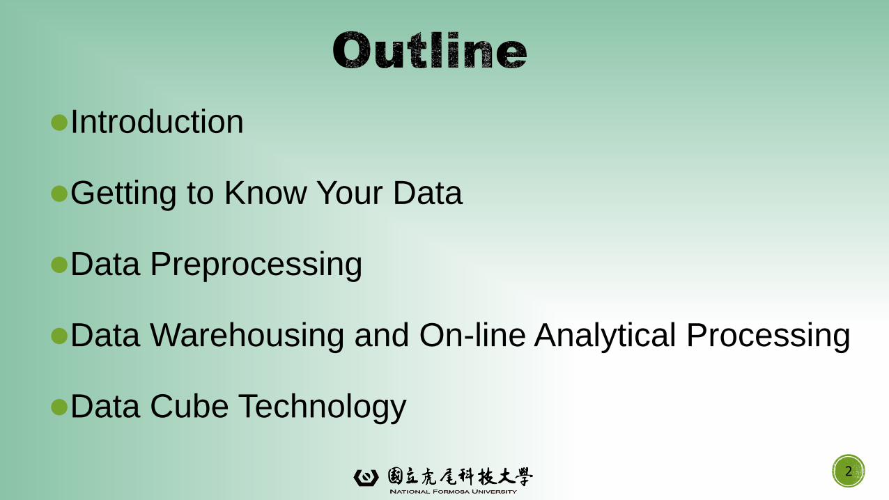
Introduction
Getting to Know Your Data
Data Preprocessing
Data Warehousing and On-line Analytical Processing
Data Cube Technology
2
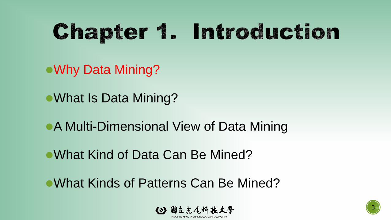
Why Data Mining?
What Is Data Mining?
A Multi-Dimensional View of Data Mining
What Kind of Data Can Be Mined?
What Kinds of Patterns Can Be Mined?
3
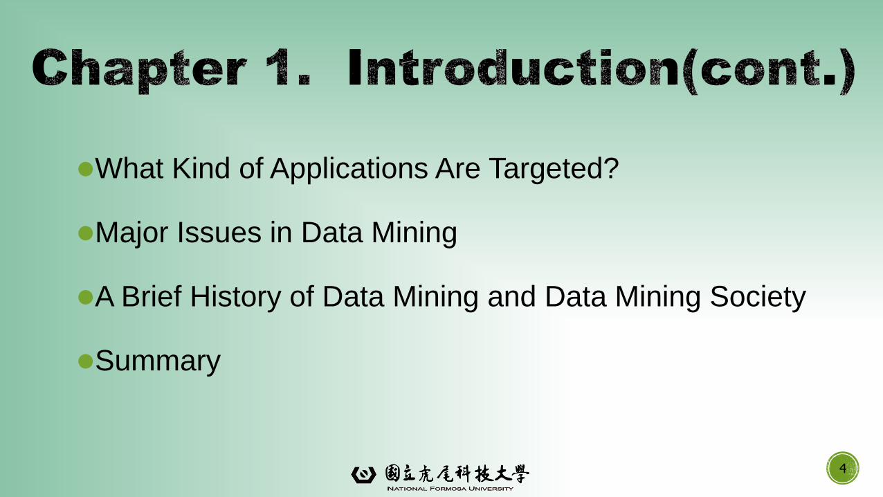
What Kind of Applications Are Targeted?
Major Issues in Data Mining
A Brief History of Data Mining and Data Mining Society
Summary
4
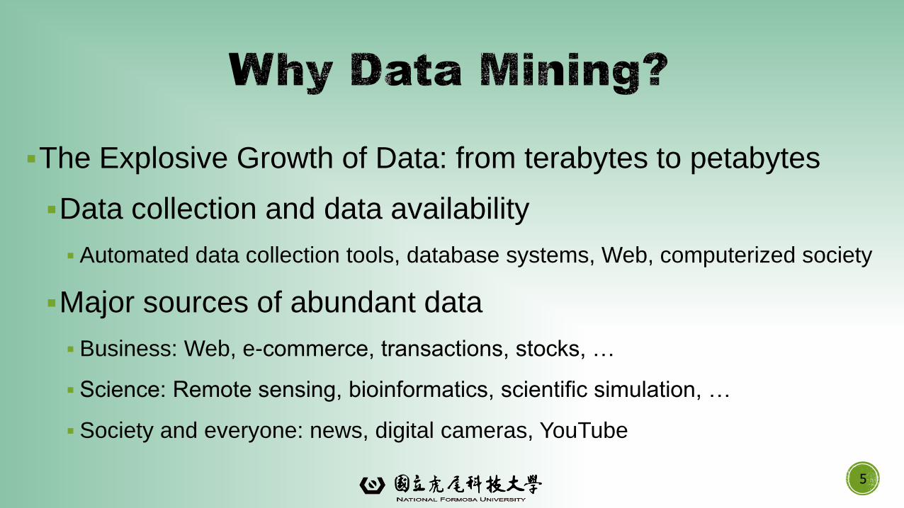
▪The Explosive Growth of Data: from terabytes to petabytes
▪Data collection and data availability
▪ Automated data collection tools, database systems, Web, computerized society
▪Major sources of abundant data
▪ Business: Web, e-commerce, transactions, stocks, …
▪ Science: Remote sensing, bioinformatics, scientific simulation, …
▪ Society and everyone: news, digital cameras, YouTube
5
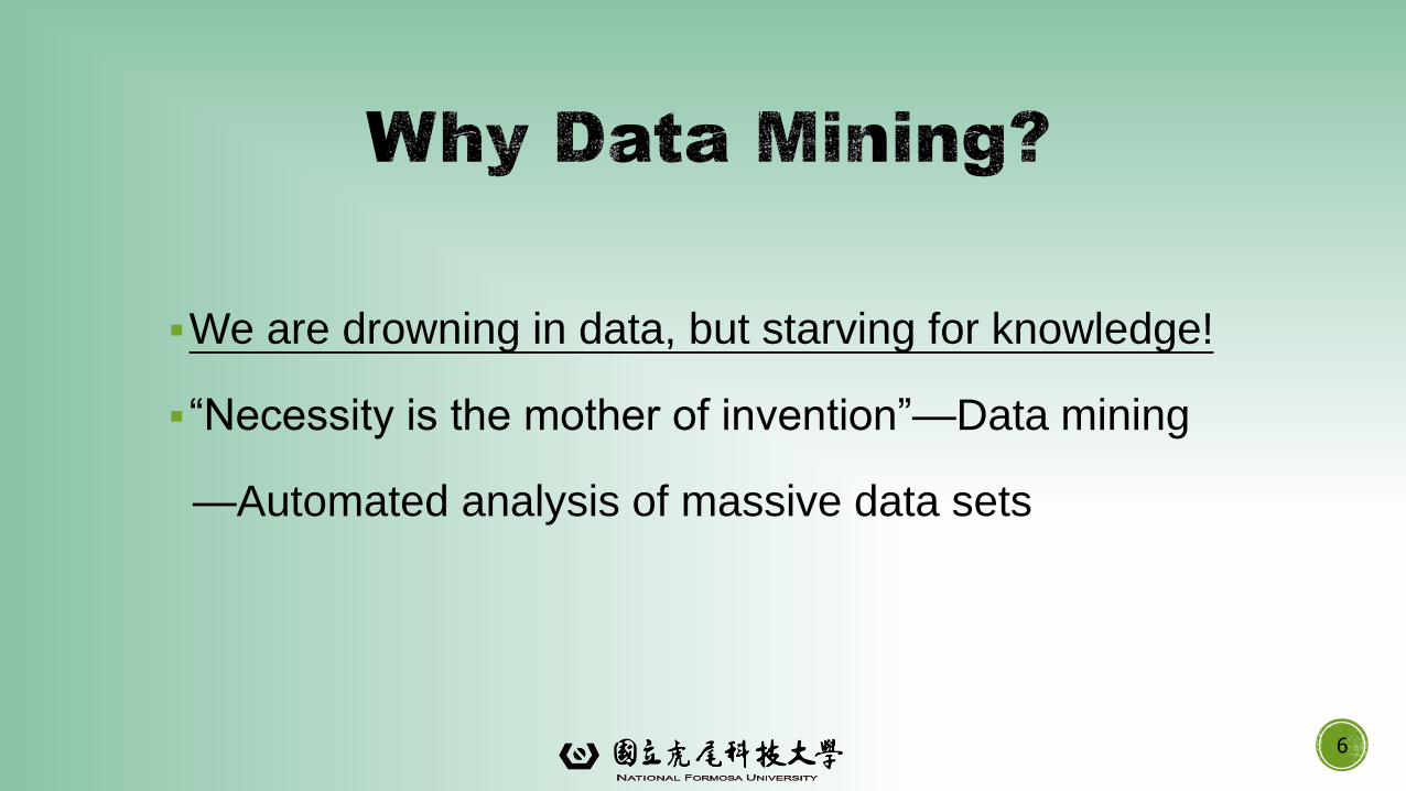
▪We are drowning in data, but starving for knowledge!
▪“Necessity is the mother of invention”—Data mining
—Automated analysis of massive data sets
6
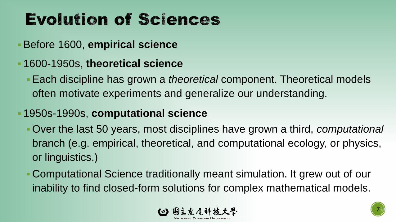
▪Before 1600, empirical science
▪1600-1950s, theoretical science
▪Each discipline has grown a theoretical component. Theoretical models
often motivate experiments and generalize our understanding.
▪1950s-1990s, computational science
▪Over the last 50 years, most disciplines have grown a third, computational
branch (e.g. empirical, theoretical, and computational ecology, or physics,
or linguistics.)
▪Computational Science traditionally meant simulation. It grew out of our
inability to find closed-form solutions for complex mathematical models.
7
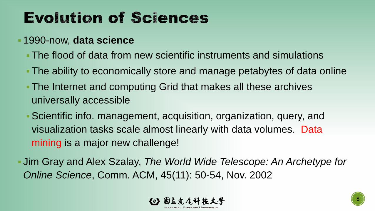
▪1990-now, data science
▪The flood of data from new scientific instruments and simulations
▪The ability to economically store and manage petabytes of data online
▪The Internet and computing Grid that makes all these archives
universally accessible
▪Scientific info. management, acquisition, organization, query, and
visualization tasks scale almost linearly with data volumes. Data
mining is a major new challenge!
▪ Jim Gray and Alex Szalay, The World Wide Telescope: An Archetype for
Online Science, Comm. ACM, 45(11): 50-54, Nov. 2002
8
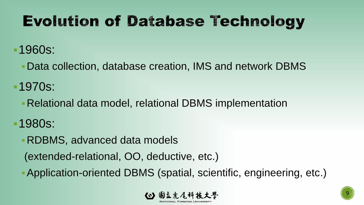
▪1960s:
▪Data collection, database creation, IMS and network DBMS
▪1970s:
▪Relational data model, relational DBMS implementation
▪1980s:
▪RDBMS, advanced data models
(extended-relational, OO, deductive, etc.)
▪Application-oriented DBMS (spatial, scientific, engineering, etc.)
9
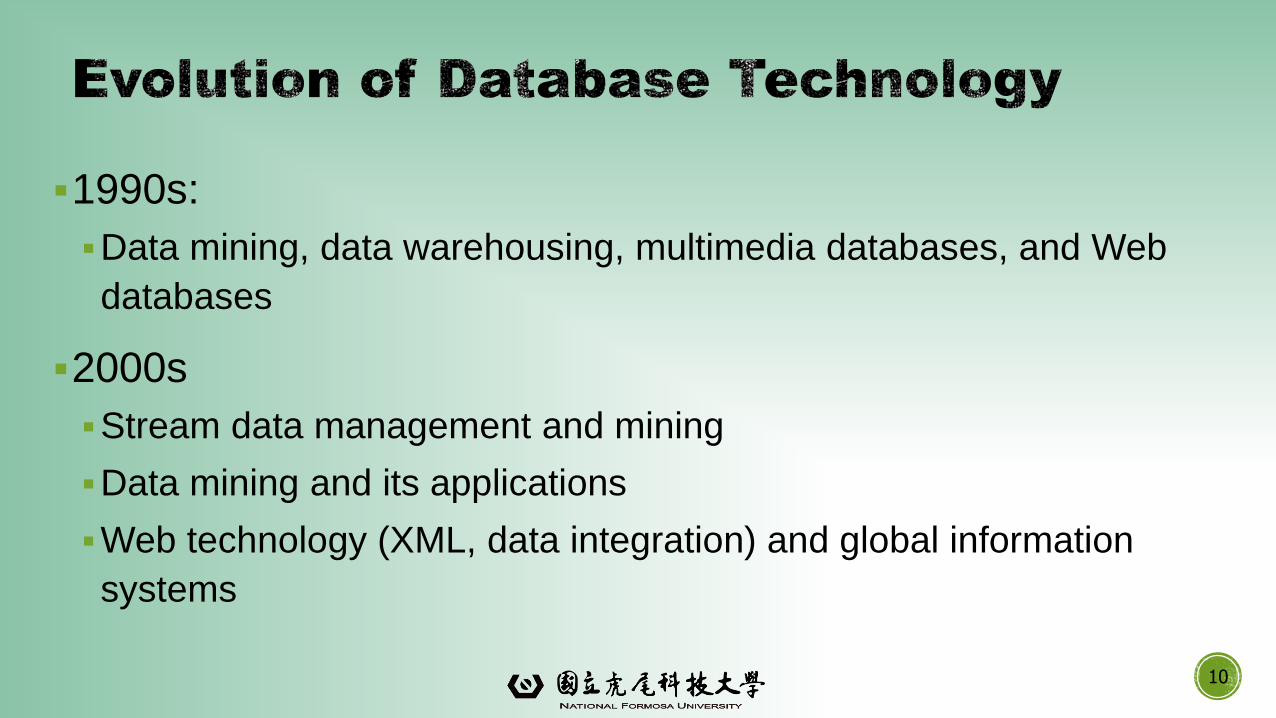
▪1990s:
▪Data mining, data warehousing, multimedia databases, and Web
databases
▪2000s
▪Stream data management and mining
▪Data mining and its applications
▪Web technology (XML, data integration) and global information
systems
10
Why Data Mining?
What Is Data Mining?
A Multi-Dimensional View of Data Mining
What Kind of Data Can Be Mined?
What Kinds of Patterns Can Be Mined?
11

What Kind of Applications Are Targeted?
Major Issues in Data Mining
A Brief History of Data Mining and Data Mining Society
Summary
12
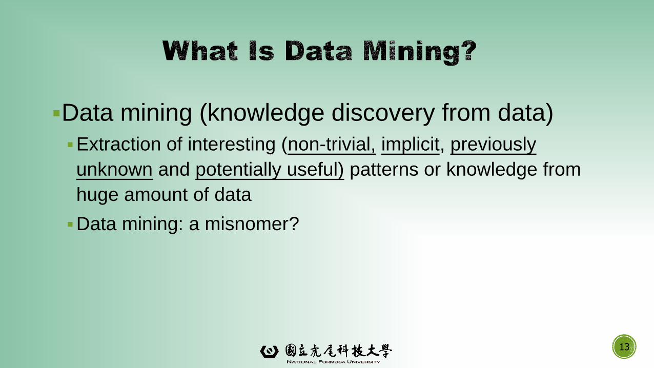
▪Data mining (knowledge discovery from data)
▪Extraction of interesting (non-trivial, implicit, previously
unknown and potentially useful) patterns or knowledge from
huge amount of data
▪Data mining: a misnomer?
13
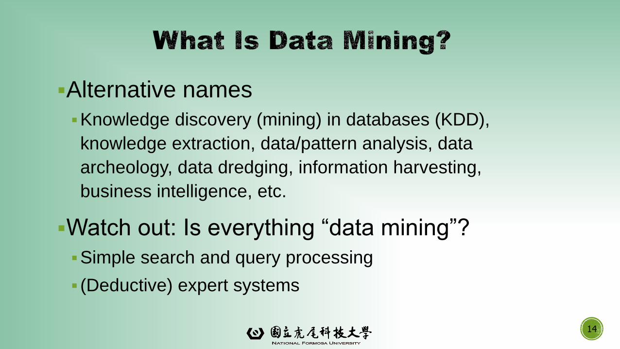
▪Alternative names
▪Knowledge discovery (mining) in databases (KDD),
knowledge extraction, data/pattern analysis, data
archeology, data dredging, information harvesting,
business intelligence, etc.
▪Watch out: Is everything “data mining”?
▪Simple search and query processing
▪ (Deductive) expert systems
14
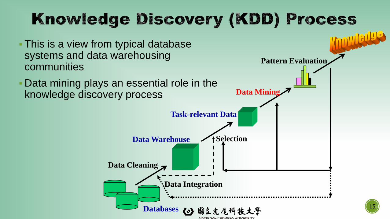
▪This is a view from typical database systems and data warehousing communities
▪Data mining plays an essential role in the knowledge discovery process
15
Data Cleaning
Data Integration
Databases
Data Warehouse
Task-relevant Data
Selection
Data Mining
Pattern Evaluation
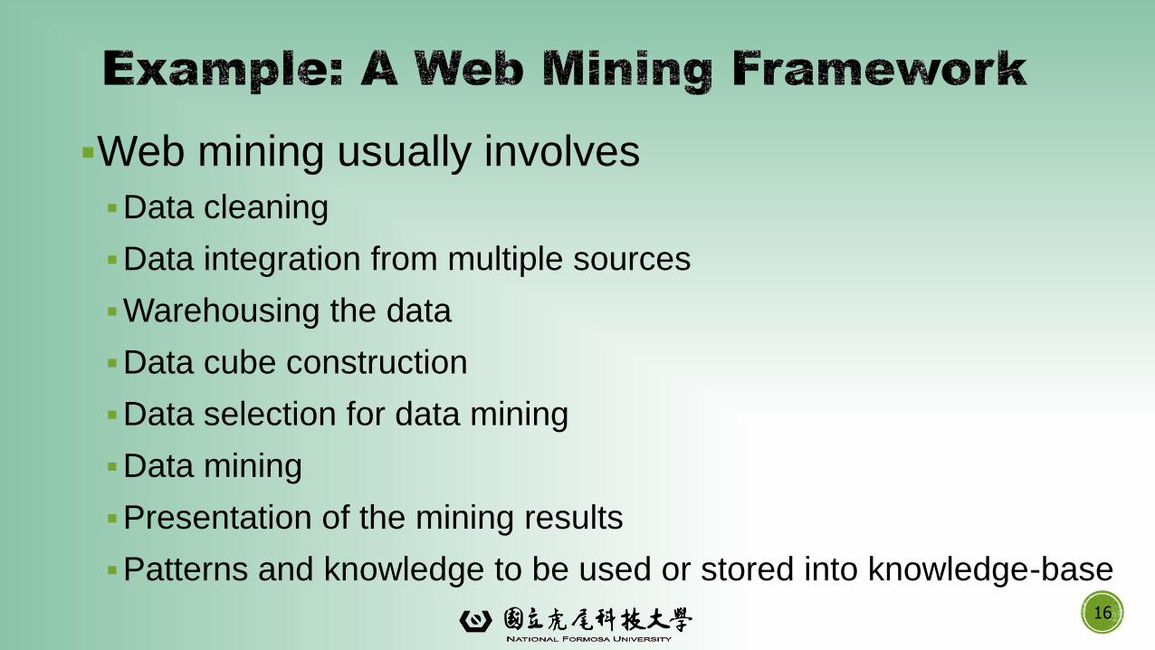
▪Web mining usually involves
▪Data cleaning
▪Data integration from multiple sources
▪Warehousing the data
▪Data cube construction
▪Data selection for data mining
▪Data mining
▪Presentation of the mining results
▪Patterns and knowledge to be used or stored into knowledge-base16
17
Increasing potential
to support
business decisions End User
Business
Analyst
Data
Analyst
DBA
DecisionMaking
Data Presentation
Visualization Techniques
Data MiningInformation Discovery
Data Exploration
Statistical Summary, Querying, and Reporting
Data Preprocessing/Integration, Data Warehouses
Data Sources
Paper, Files, Web documents, Scientific experiments, Database Systems
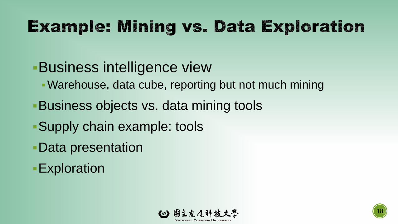
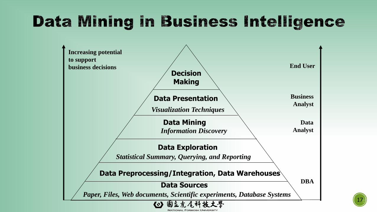
▪Business intelligence view▪Warehouse, data cube, reporting but not much mining
▪Business objects vs. data mining tools
▪Supply chain example: tools
▪Data presentation
▪Exploration
18
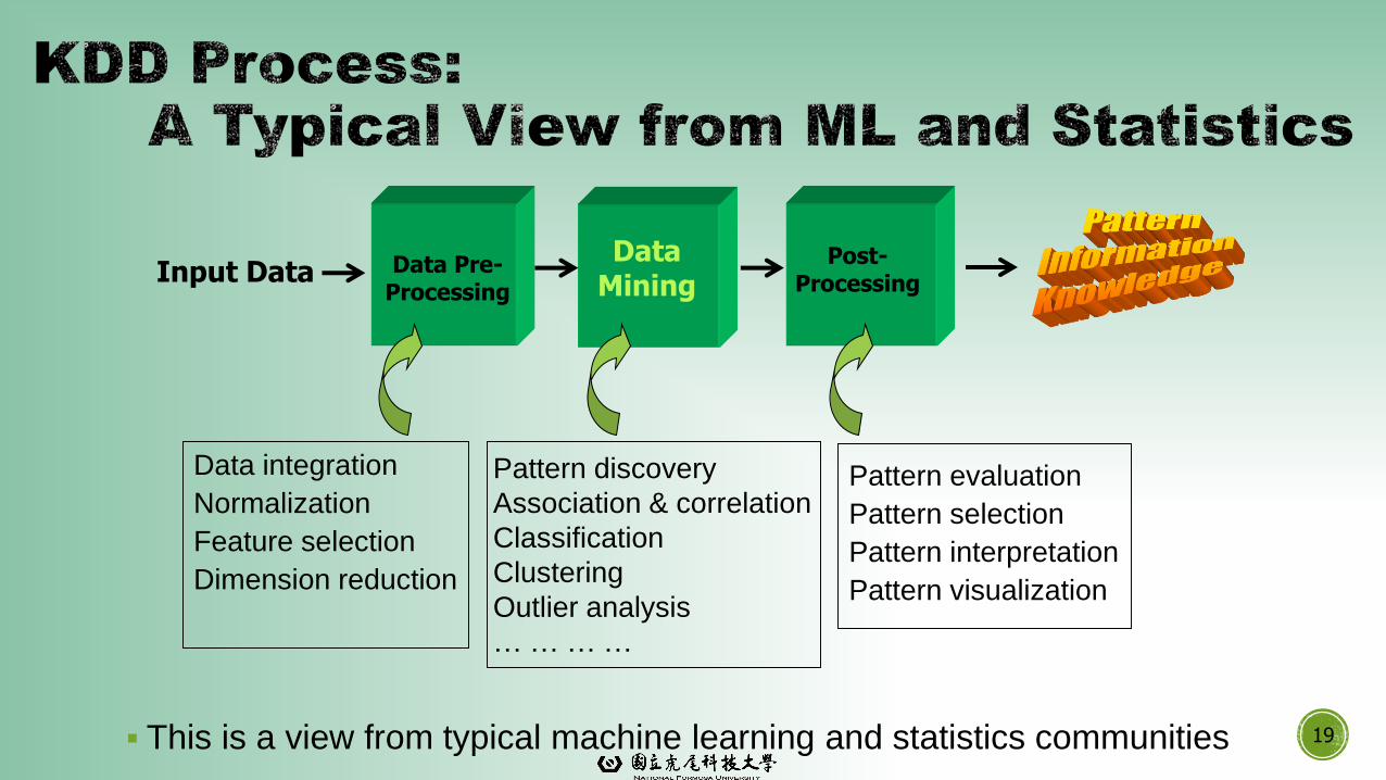
▪ This is a view from typical machine learning and statistics communities 19
Input DataData
MiningData Pre-
Processing
Post-Processing
Data integration
Normalization
Feature selection
Dimension reduction
Pattern discovery
Association & correlation
Classification
Clustering
Outlier analysis
… … … …
Pattern evaluation
Pattern selection
Pattern interpretation
Pattern visualization
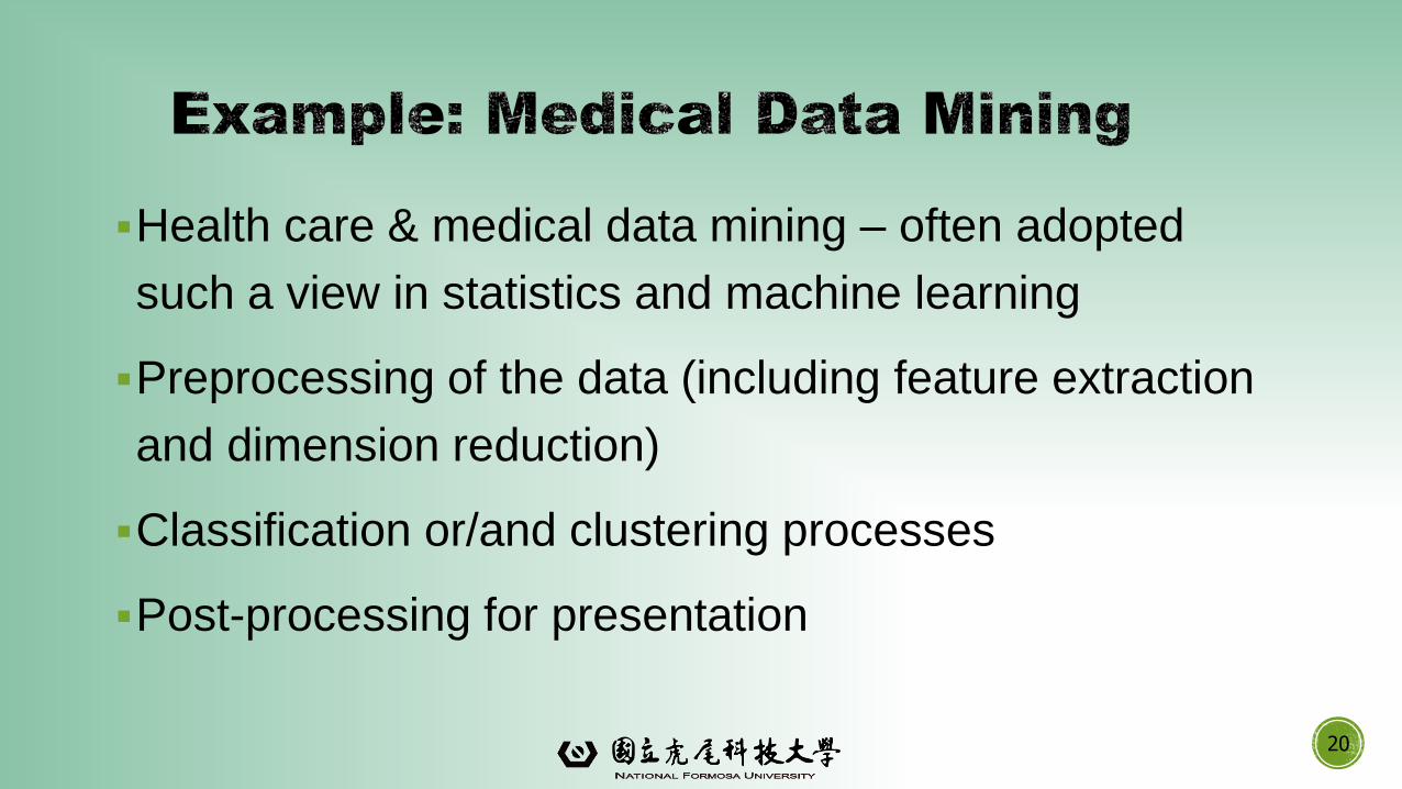
▪Health care & medical data mining – often adopted
such a view in statistics and machine learning
▪Preprocessing of the data (including feature extraction
and dimension reduction)
▪Classification or/and clustering processes
▪Post-processing for presentation
20
Why Data Mining?
What Is Data Mining?
A Multi-Dimensional View of Data Mining
What Kind of Data Can Be Mined?
What Kinds of Patterns Can Be Mined?
21

What Kind of Applications Are Targeted?
Major Issues in Data Mining
A Brief History of Data Mining and Data Mining Society
Summary
22
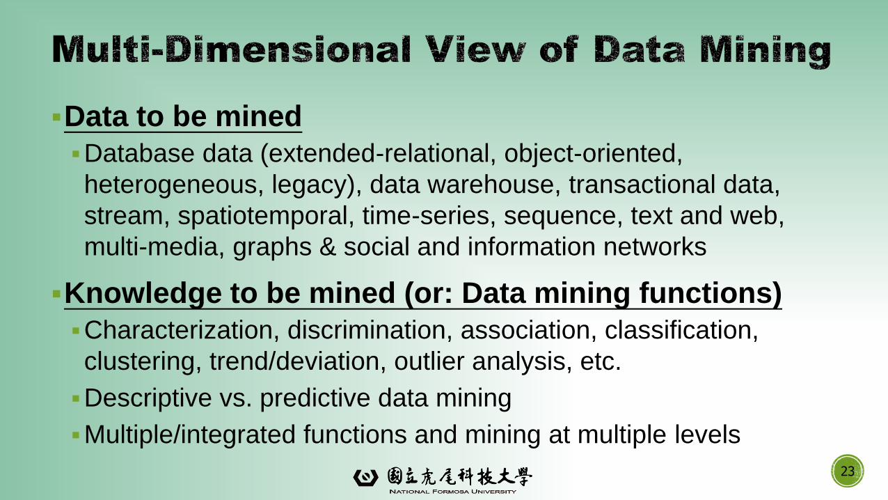
▪Data to be mined
▪Database data (extended-relational, object-oriented,
heterogeneous, legacy), data warehouse, transactional data,
stream, spatiotemporal, time-series, sequence, text and web,
multi-media, graphs & social and information networks
▪Knowledge to be mined (or: Data mining functions)
▪Characterization, discrimination, association, classification,
clustering, trend/deviation, outlier analysis, etc.
▪Descriptive vs. predictive data mining
▪Multiple/integrated functions and mining at multiple levels
23
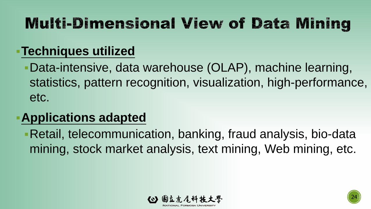
▪Techniques utilized
▪Data-intensive, data warehouse (OLAP), machine learning,
statistics, pattern recognition, visualization, high-performance,
etc.
▪Applications adapted
▪Retail, telecommunication, banking, fraud analysis, bio-data
mining, stock market analysis, text mining, Web mining, etc.
24
Why Data Mining?
What Is Data Mining?
A Multi-Dimensional View of Data Mining
What Kind of Data Can Be Mined?
What Kinds of Patterns Can Be Mined?
25

What Kind of Applications Are Targeted?
Major Issues in Data Mining
A Brief History of Data Mining and Data Mining Society
Summary
26
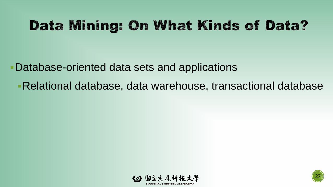
▪Database-oriented data sets and applications
▪Relational database, data warehouse, transactional database
27
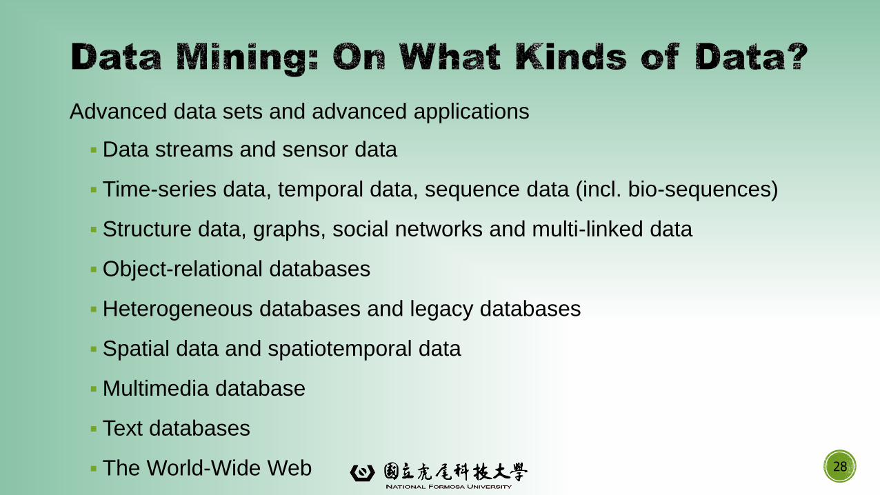
Advanced data sets and advanced applications
▪Data streams and sensor data
▪ Time-series data, temporal data, sequence data (incl. bio-sequences)
▪ Structure data, graphs, social networks and multi-linked data
▪Object-relational databases
▪Heterogeneous databases and legacy databases
▪ Spatial data and spatiotemporal data
▪Multimedia database
▪ Text databases
▪ The World-Wide Web 28
Why Data Mining?
What Is Data Mining?
A Multi-Dimensional View of Data Mining
What Kind of Data Can Be Mined?
What Kinds of Patterns Can Be Mined?
29

What Kind of Applications Are Targeted?
Major Issues in Data Mining
A Brief History of Data Mining and Data Mining Society
Summary
30
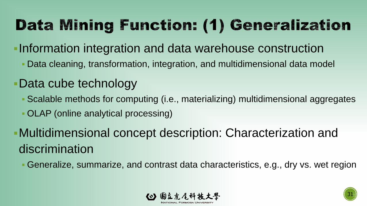
▪Information integration and data warehouse construction
▪Data cleaning, transformation, integration, and multidimensional data model
▪Data cube technology
▪ Scalable methods for computing (i.e., materializing) multidimensional aggregates
▪OLAP (online analytical processing)
▪Multidimensional concept description: Characterization and
discrimination
▪Generalize, summarize, and contrast data characteristics, e.g., dry vs. wet region
31
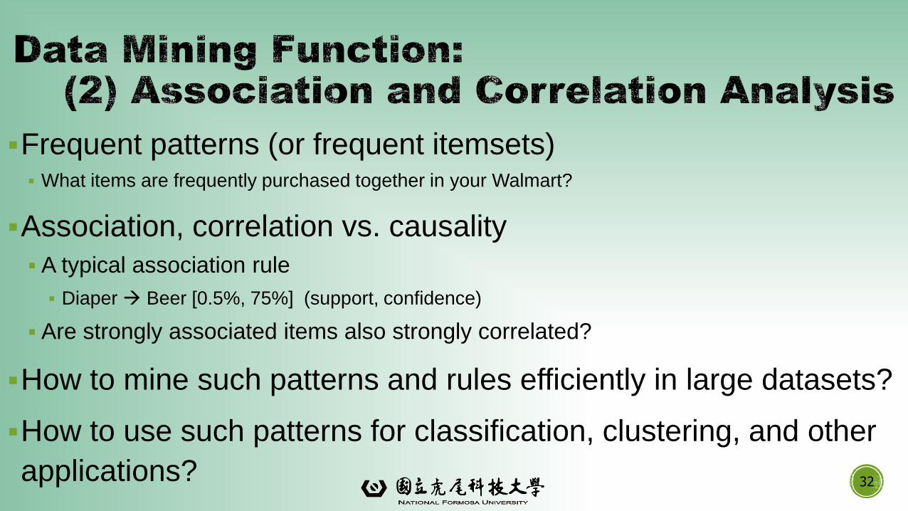
▪Frequent patterns (or frequent itemsets)▪ What items are frequently purchased together in your Walmart?
▪Association, correlation vs. causality
▪ A typical association rule
▪ Diaper Beer [0.5%, 75%] (support, confidence)
▪ Are strongly associated items also strongly correlated?
▪How to mine such patterns and rules efficiently in large datasets?
▪How to use such patterns for classification, clustering, and other
applications? 32
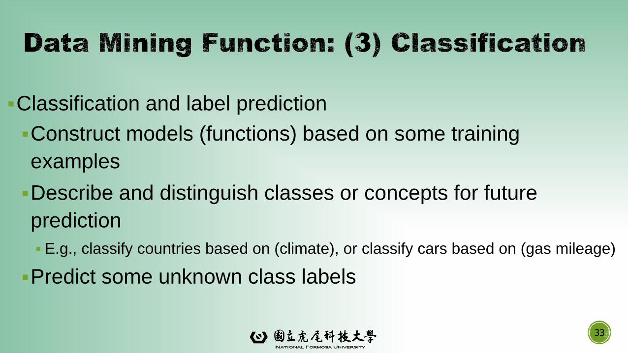
▪Classification and label prediction
▪Construct models (functions) based on some training
examples
▪Describe and distinguish classes or concepts for future
prediction
▪ E.g., classify countries based on (climate), or classify cars based on (gas mileage)
▪Predict some unknown class labels
33
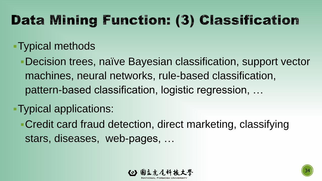
▪Typical methods
▪Decision trees, naïve Bayesian classification, support vector
machines, neural networks, rule-based classification,
pattern-based classification, logistic regression, …
▪Typical applications:
▪Credit card fraud detection, direct marketing, classifying
stars, diseases, web-pages, …
34
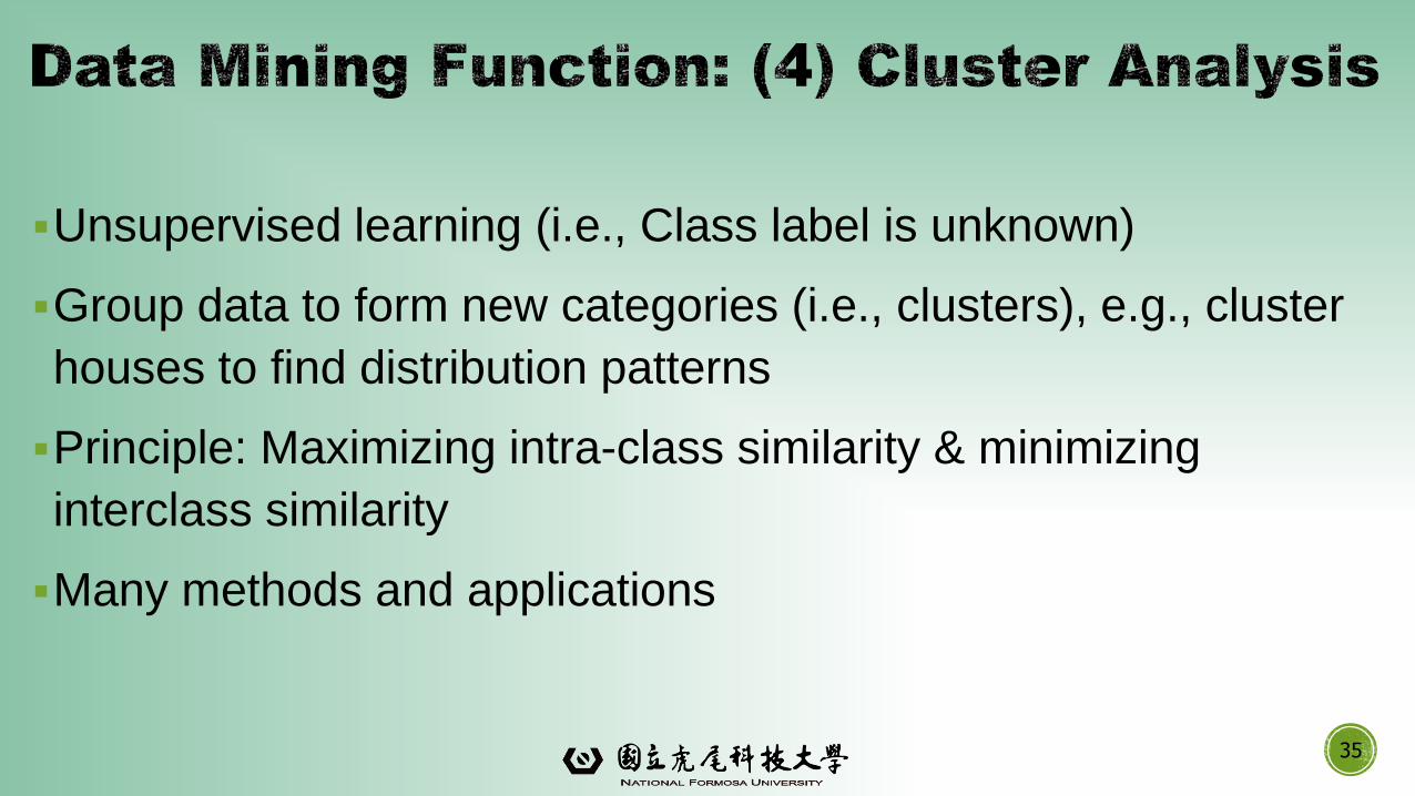
▪Unsupervised learning (i.e., Class label is unknown)
▪Group data to form new categories (i.e., clusters), e.g., cluster
houses to find distribution patterns
▪Principle: Maximizing intra-class similarity & minimizing
interclass similarity
▪Many methods and applications
35
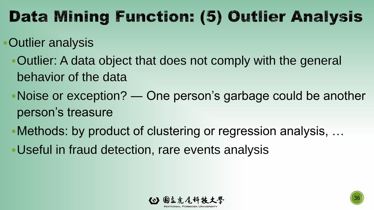
▪Outlier analysis
▪Outlier: A data object that does not comply with the general
behavior of the data
▪Noise or exception? ― One person’s garbage could be another
person’s treasure
▪Methods: by product of clustering or regression analysis, …
▪Useful in fraud detection, rare events analysis
36
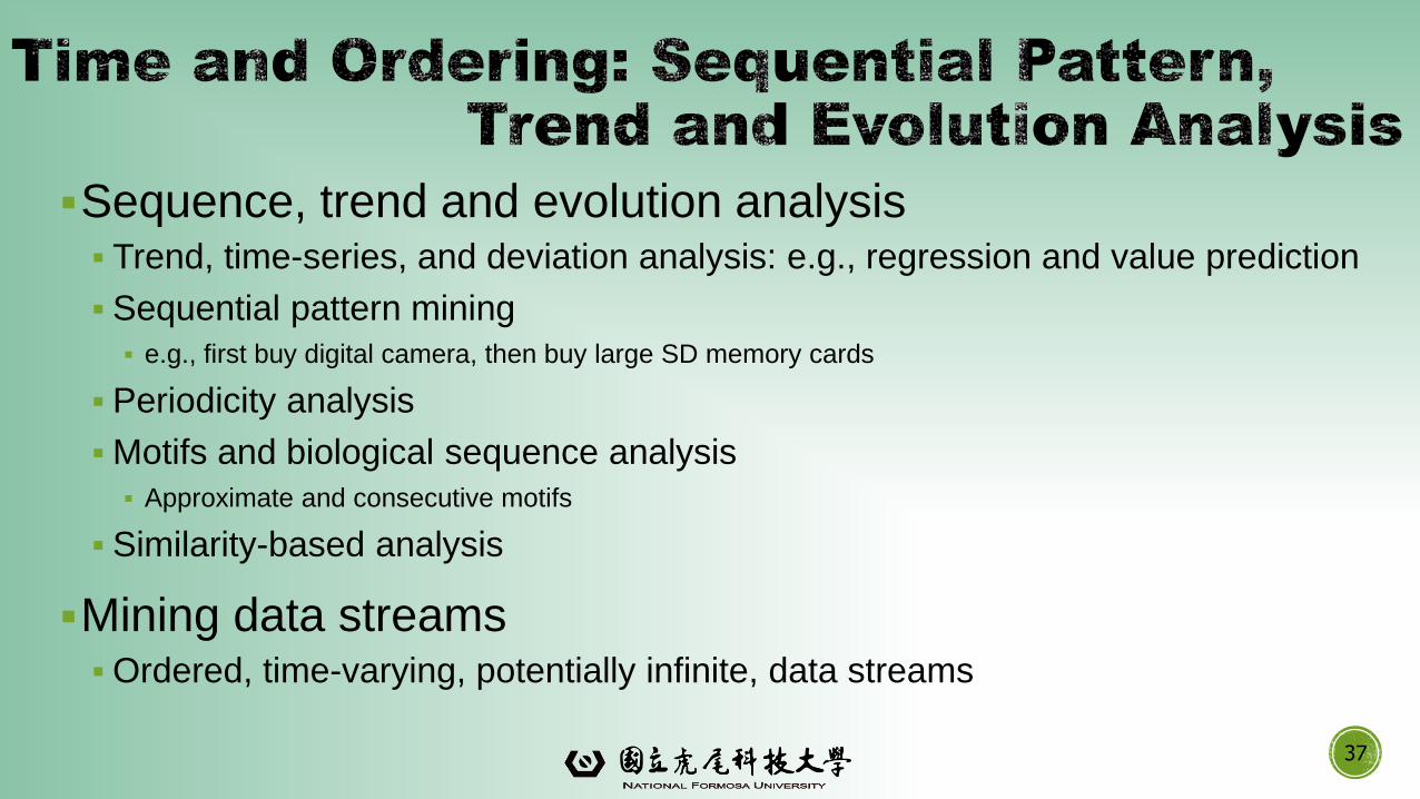
▪Sequence, trend and evolution analysis▪ Trend, time-series, and deviation analysis: e.g., regression and value prediction
▪ Sequential pattern mining
▪ e.g., first buy digital camera, then buy large SD memory cards
▪ Periodicity analysis
▪Motifs and biological sequence analysis
▪ Approximate and consecutive motifs
▪ Similarity-based analysis
▪Mining data streams▪Ordered, time-varying, potentially infinite, data streams
37
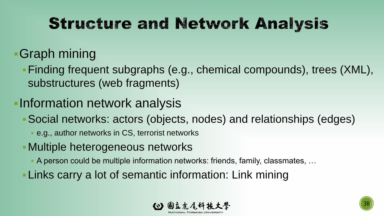
▪Graph mining
▪Finding frequent subgraphs (e.g., chemical compounds), trees (XML),
substructures (web fragments)
▪Information network analysis
▪Social networks: actors (objects, nodes) and relationships (edges)▪ e.g., author networks in CS, terrorist networks
▪Multiple heterogeneous networks▪ A person could be multiple information networks: friends, family, classmates, …
▪Links carry a lot of semantic information: Link mining
38
▪Web mining▪Web is a big information network: from PageRank to Google
▪Analysis of Web information networks
▪Web community discovery, opinion mining, usage mining, …
39
▪Are all mined knowledge interesting?
▪One can mine tremendous amount of “patterns” and knowledge
▪Some may fit only certain dimension space (time, location, …)
▪Some may not be representative, may be transient, …
40
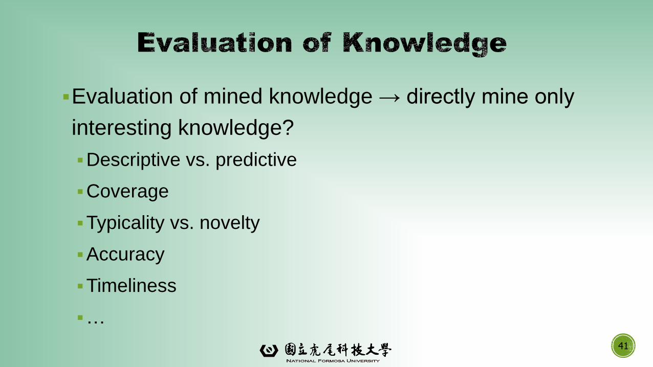
▪Evaluation of mined knowledge → directly mine only
interesting knowledge?
▪Descriptive vs. predictive
▪Coverage
▪Typicality vs. novelty
▪Accuracy
▪Timeliness
▪…
41

Why Data Mining?
What Is Data Mining?
A Multi-Dimensional View of Data Mining
What Kind of Data Can Be Mined?
What Kinds of Patterns Can Be Mined?
42

What Kind of Applications Are Targeted?
Major Issues in Data Mining
A Brief History of Data Mining and Data Mining Society
Summary
43
What Technology Are Used?
What Kind of Applications Are Targeted?
Major Issues in Data Mining
A Brief History of Data Mining and Data Mining Society
Summary
44
45
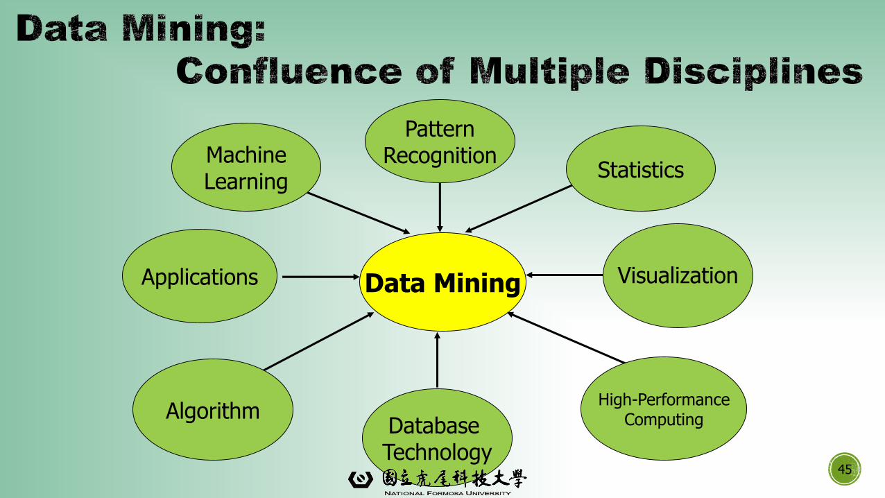
Data Mining
MachineLearning
Statistics
Applications
AlgorithmHigh-Performance
Computing
Visualization
Database Technology
PatternRecognition
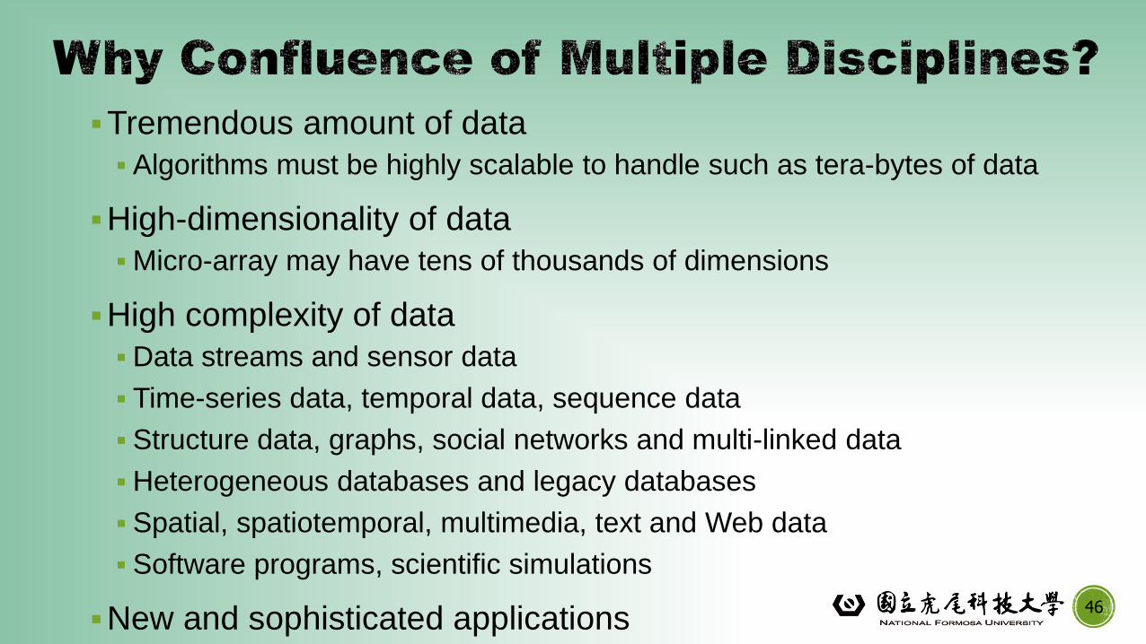
▪Tremendous amount of data
▪ Algorithms must be highly scalable to handle such as tera-bytes of data
▪High-dimensionality of data
▪Micro-array may have tens of thousands of dimensions
▪High complexity of data
▪Data streams and sensor data
▪ Time-series data, temporal data, sequence data
▪ Structure data, graphs, social networks and multi-linked data
▪Heterogeneous databases and legacy databases
▪ Spatial, spatiotemporal, multimedia, text and Web data
▪ Software programs, scientific simulations
▪New and sophisticated applications46

Why Data Mining?
What Is Data Mining?
A Multi-Dimensional View of Data Mining
What Kind of Data Can Be Mined?
What Kinds of Patterns Can Be Mined?
47
What Technology Are Used?
What Kind of Applications Are Targeted?
Major Issues in Data Mining
A Brief History of Data Mining and Data Mining Society
Summary
48
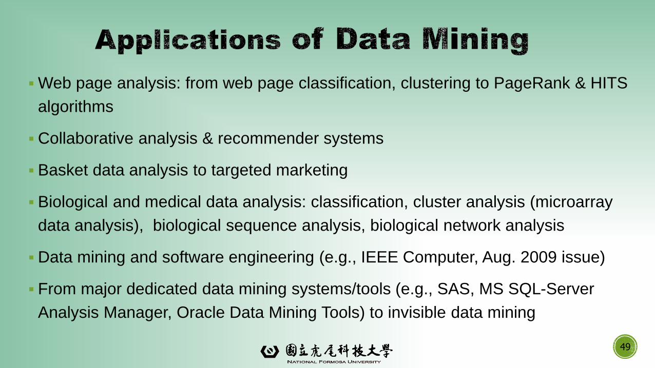
▪Web page analysis: from web page classification, clustering to PageRank & HITS
algorithms
▪Collaborative analysis & recommender systems
▪ Basket data analysis to targeted marketing
▪ Biological and medical data analysis: classification, cluster analysis (microarray
data analysis), biological sequence analysis, biological network analysis
▪Data mining and software engineering (e.g., IEEE Computer, Aug. 2009 issue)
▪ From major dedicated data mining systems/tools (e.g., SAS, MS SQL-Server
Analysis Manager, Oracle Data Mining Tools) to invisible data mining
49

Why Data Mining?
What Is Data Mining?
A Multi-Dimensional View of Data Mining
What Kind of Data Can Be Mined?
What Kinds of Patterns Can Be Mined?
50
What Technology Are Used?
What Kind of Applications Are Targeted?
Major Issues in Data Mining
A Brief History of Data Mining and Data Mining Society
Summary
51
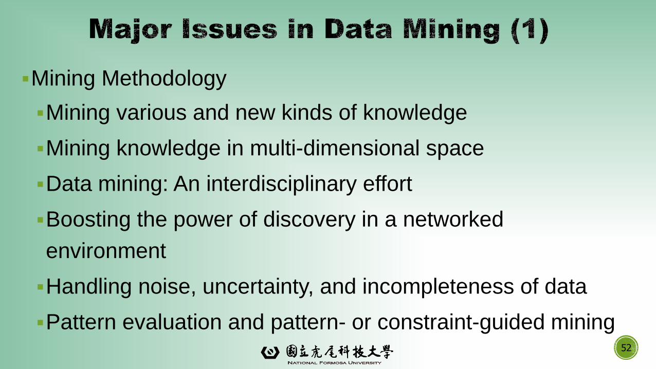
▪Mining Methodology
▪Mining various and new kinds of knowledge
▪Mining knowledge in multi-dimensional space
▪Data mining: An interdisciplinary effort
▪Boosting the power of discovery in a networked
environment
▪Handling noise, uncertainty, and incompleteness of data
▪Pattern evaluation and pattern- or constraint-guided mining52
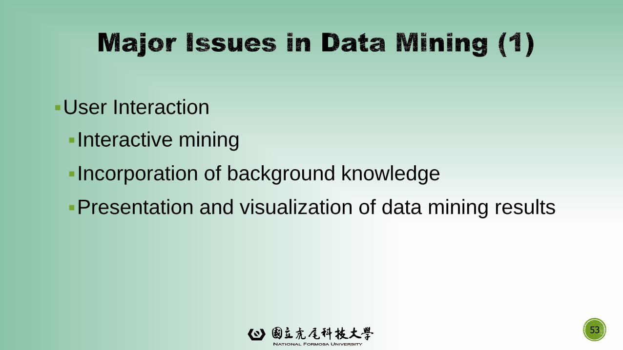
▪User Interaction
▪Interactive mining
▪Incorporation of background knowledge
▪Presentation and visualization of data mining results
53
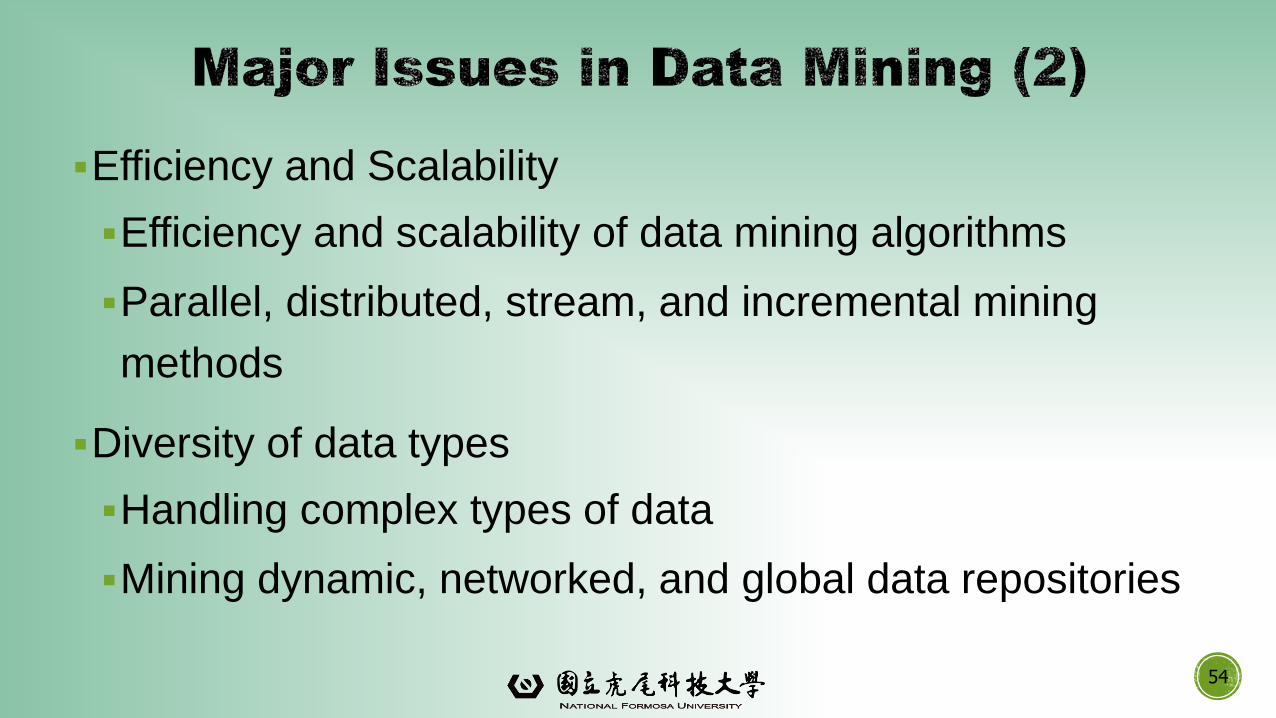
▪Efficiency and Scalability
▪Efficiency and scalability of data mining algorithms
▪Parallel, distributed, stream, and incremental mining
methods
▪Diversity of data types
▪Handling complex types of data
▪Mining dynamic, networked, and global data repositories
54
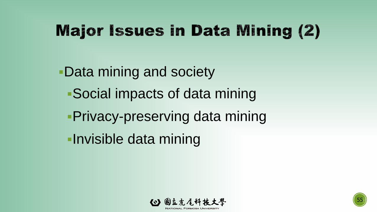
▪Data mining and society
▪Social impacts of data mining
▪Privacy-preserving data mining
▪Invisible data mining
55
Why Data Mining?
What Is Data Mining?
A Multi-Dimensional View of Data Mining
What Kind of Data Can Be Mined?
What Kinds of Patterns Can Be Mined?
56
What Technology Are Used?
What Kind of Applications Are Targeted?
Major Issues in Data Mining
A Brief History of Data Mining and Data Mining Society
Summary
57
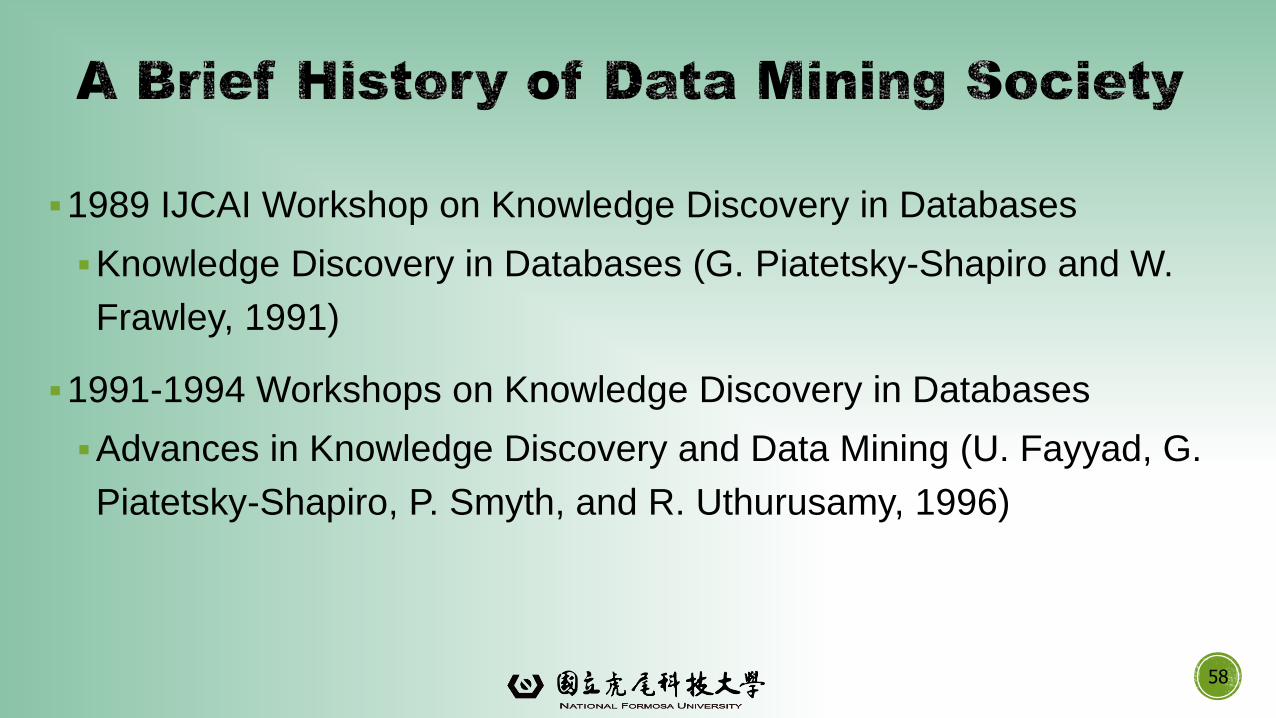
▪1989 IJCAI Workshop on Knowledge Discovery in Databases
▪Knowledge Discovery in Databases (G. Piatetsky-Shapiro and W.
Frawley, 1991)
▪1991-1994 Workshops on Knowledge Discovery in Databases
▪Advances in Knowledge Discovery and Data Mining (U. Fayyad, G.
Piatetsky-Shapiro, P. Smyth, and R. Uthurusamy, 1996)
58
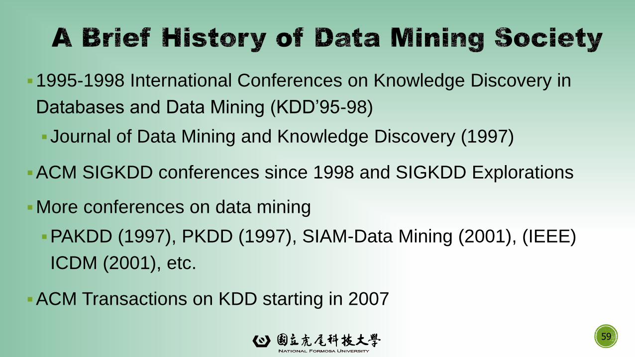
▪1995-1998 International Conferences on Knowledge Discovery in
Databases and Data Mining (KDD’95-98)
▪Journal of Data Mining and Knowledge Discovery (1997)
▪ACM SIGKDD conferences since 1998 and SIGKDD Explorations
▪More conferences on data mining
▪PAKDD (1997), PKDD (1997), SIAM-Data Mining (2001), (IEEE)
ICDM (2001), etc.
▪ACM Transactions on KDD starting in 2007
59
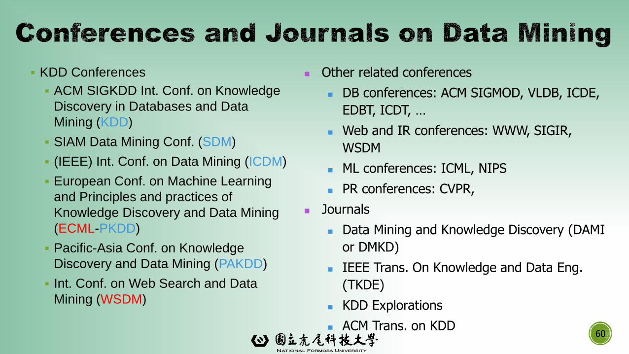
▪ KDD Conferences
▪ ACM SIGKDD Int. Conf. on Knowledge
Discovery in Databases and Data
Mining (KDD)
▪ SIAM Data Mining Conf. (SDM)
▪ (IEEE) Int. Conf. on Data Mining (ICDM)
▪ European Conf. on Machine Learning
and Principles and practices of
Knowledge Discovery and Data Mining
(ECML-PKDD)
▪ Pacific-Asia Conf. on Knowledge
Discovery and Data Mining (PAKDD)
▪ Int. Conf. on Web Search and Data
Mining (WSDM)
60
Other related conferences
DB conferences: ACM SIGMOD, VLDB, ICDE,
EDBT, ICDT, …
Web and IR conferences: WWW, SIGIR,
WSDM
ML conferences: ICML, NIPS
PR conferences: CVPR,
Journals
Data Mining and Knowledge Discovery (DAMI
or DMKD)
IEEE Trans. On Knowledge and Data Eng.
(TKDE)
KDD Explorations
ACM Trans. on KDD
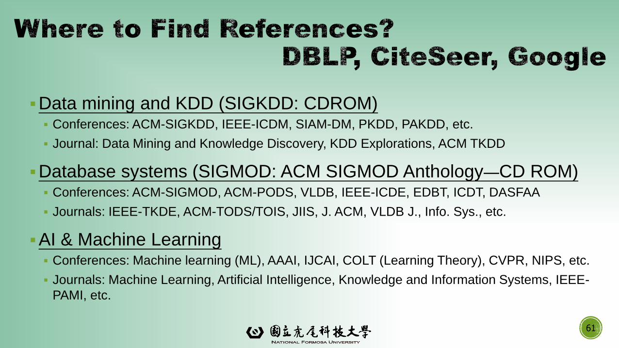
▪Data mining and KDD (SIGKDD: CDROM)▪ Conferences: ACM-SIGKDD, IEEE-ICDM, SIAM-DM, PKDD, PAKDD, etc.
▪ Journal: Data Mining and Knowledge Discovery, KDD Explorations, ACM TKDD
▪Database systems (SIGMOD: ACM SIGMOD Anthology—CD ROM)▪ Conferences: ACM-SIGMOD, ACM-PODS, VLDB, IEEE-ICDE, EDBT, ICDT, DASFAA
▪ Journals: IEEE-TKDE, ACM-TODS/TOIS, JIIS, J. ACM, VLDB J., Info. Sys., etc.
▪AI & Machine Learning▪ Conferences: Machine learning (ML), AAAI, IJCAI, COLT (Learning Theory), CVPR, NIPS, etc.
▪ Journals: Machine Learning, Artificial Intelligence, Knowledge and Information Systems, IEEE-
PAMI, etc.
61
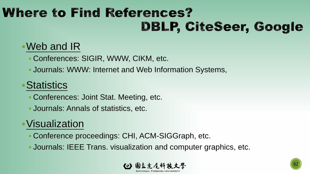
▪Web and IR▪Conferences: SIGIR, WWW, CIKM, etc.
▪ Journals: WWW: Internet and Web Information Systems,
▪Statistics▪Conferences: Joint Stat. Meeting, etc.
▪ Journals: Annals of statistics, etc.
▪Visualization▪Conference proceedings: CHI, ACM-SIGGraph, etc.
▪ Journals: IEEE Trans. visualization and computer graphics, etc.
62

Why Data Mining?
What Is Data Mining?
A Multi-Dimensional View of Data Mining
What Kind of Data Can Be Mined?
What Kinds of Patterns Can Be Mined?
63
What Technology Are Used?
What Kind of Applications Are Targeted?
Major Issues in Data Mining
A Brief History of Data Mining and Data Mining Society
Summary
64
▪Data mining: Discovering interesting patterns and
knowledge from massive amount of data
▪A natural evolution of database technology, in great
demand, with wide applications
▪A KDD process includes data cleaning, data integration,
data selection, transformation, data mining, pattern
evaluation, and knowledge presentation
65
▪Mining can be performed in a variety of data
▪Data mining functionalities: characterization, discrimination,
association, classification, clustering, outlier and trend
analysis, etc.
▪Data mining technologies and applications
▪Major issues in data mining
66
Data Objects and Attribute Types
Basic Statistical Descriptions of Data
Data Visualization
Measuring Data Similarity and Dissimilarity
Summary
67
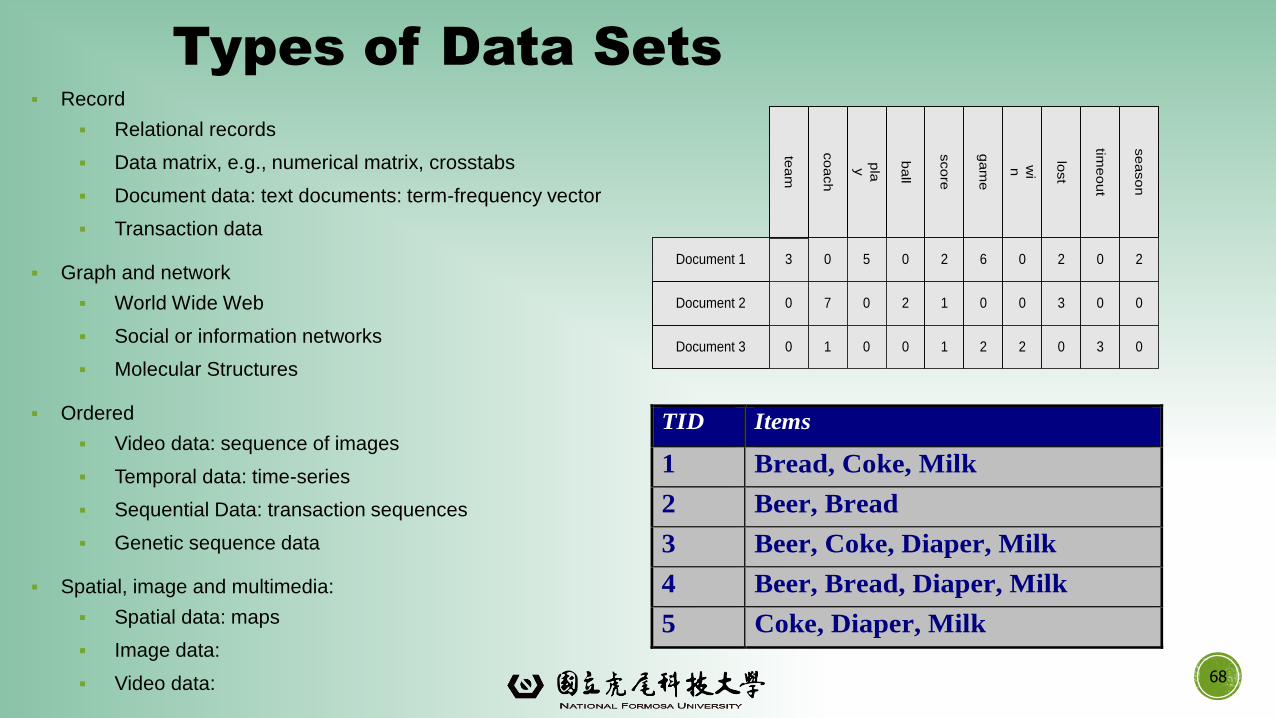
Types of Data Sets
▪ Record
▪ Relational records
▪ Data matrix, e.g., numerical matrix, crosstabs
▪ Document data: text documents: term-frequency vector
▪ Transaction data
▪ Graph and network
▪ World Wide Web
▪ Social or information networks
▪ Molecular Structures
▪ Ordered
▪ Video data: sequence of images
▪ Temporal data: time-series
▪ Sequential Data: transaction sequences
▪ Genetic sequence data
▪ Spatial, image and multimedia:
▪ Spatial data: maps
▪ Image data:
▪ Video data:
Document 1
se
aso
n
time
ou
t
lost
wi
n
ga
me
sco
re
ba
ll
play
co
ach
tea
m
Document 2
Document 3
3 0 5 0 2 6 0 2 0 2
0
0
7 0 2 1 0 0 3 0 0
1 0 0 1 2 2 0 3 0
TID Items
1 Bread, Coke, Milk
2 Beer, Bread
3 Beer, Coke, Diaper, Milk
4 Beer, Bread, Diaper, Milk
5 Coke, Diaper, Milk
68
▪ Dimensionality
▪ Curse of dimensionality
▪ Sparsity
▪ Only presence counts
▪ Resolution
▪ Patterns depend on the scale
▪ Distribution
▪ Centrality and dispersion69
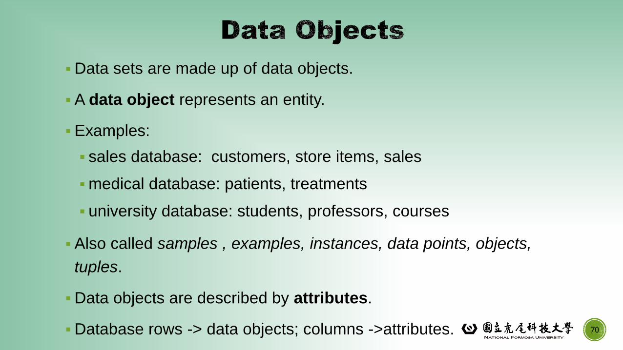
▪Data sets are made up of data objects.
▪A data object represents an entity.
▪Examples:
▪ sales database: customers, store items, sales
▪medical database: patients, treatments
▪ university database: students, professors, courses
▪Also called samples , examples, instances, data points, objects,
tuples.
▪Data objects are described by attributes.
▪Database rows -> data objects; columns ->attributes. 70
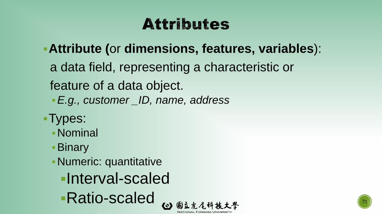
▪Attribute (or dimensions, features, variables):
a data field, representing a characteristic or
feature of a data object.▪E.g., customer _ID, name, address
▪Types:▪Nominal
▪Binary
▪Numeric: quantitative
▪Interval-scaled
▪Ratio-scaled 71
Attribute Types
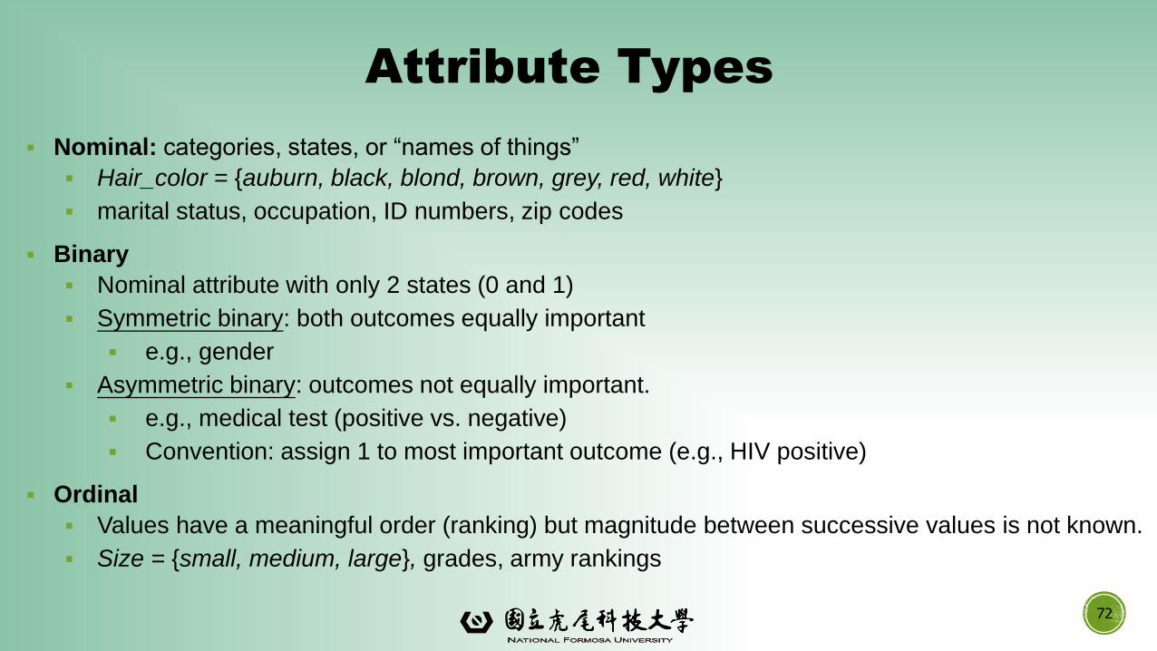
▪ Nominal: categories, states, or “names of things”
▪ Hair_color = {auburn, black, blond, brown, grey, red, white}
▪ marital status, occupation, ID numbers, zip codes
▪ Binary
▪ Nominal attribute with only 2 states (0 and 1)
▪ Symmetric binary: both outcomes equally important
▪ e.g., gender
▪ Asymmetric binary: outcomes not equally important.
▪ e.g., medical test (positive vs. negative)
▪ Convention: assign 1 to most important outcome (e.g., HIV positive)
▪ Ordinal
▪ Values have a meaningful order (ranking) but magnitude between successive values is not known.
▪ Size = {small, medium, large}, grades, army rankings
72
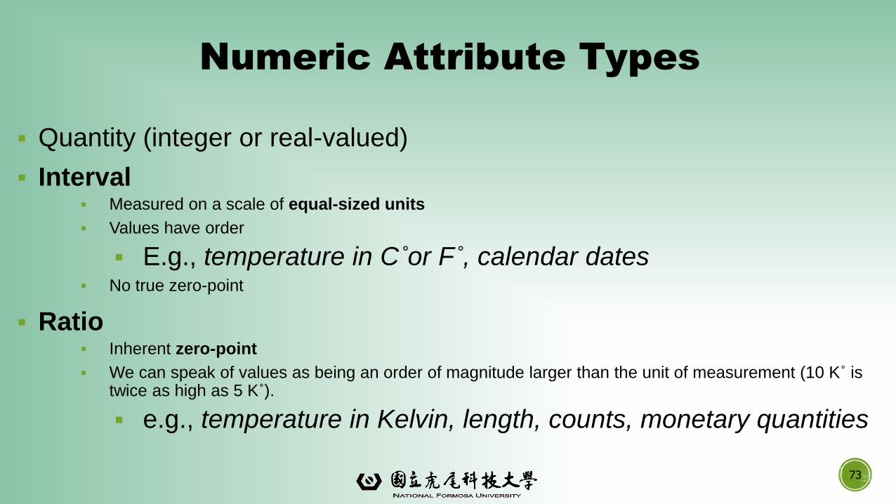
Numeric Attribute Types
▪ Quantity (integer or real-valued)
▪ Interval▪ Measured on a scale of equal-sized units
▪ Values have order
▪ E.g., temperature in C˚or F˚, calendar dates▪ No true zero-point
▪ Ratio▪ Inherent zero-point
▪ We can speak of values as being an order of magnitude larger than the unit of measurement (10 K˚ is twice as high as 5 K˚).
▪ e.g., temperature in Kelvin, length, counts, monetary quantities
73
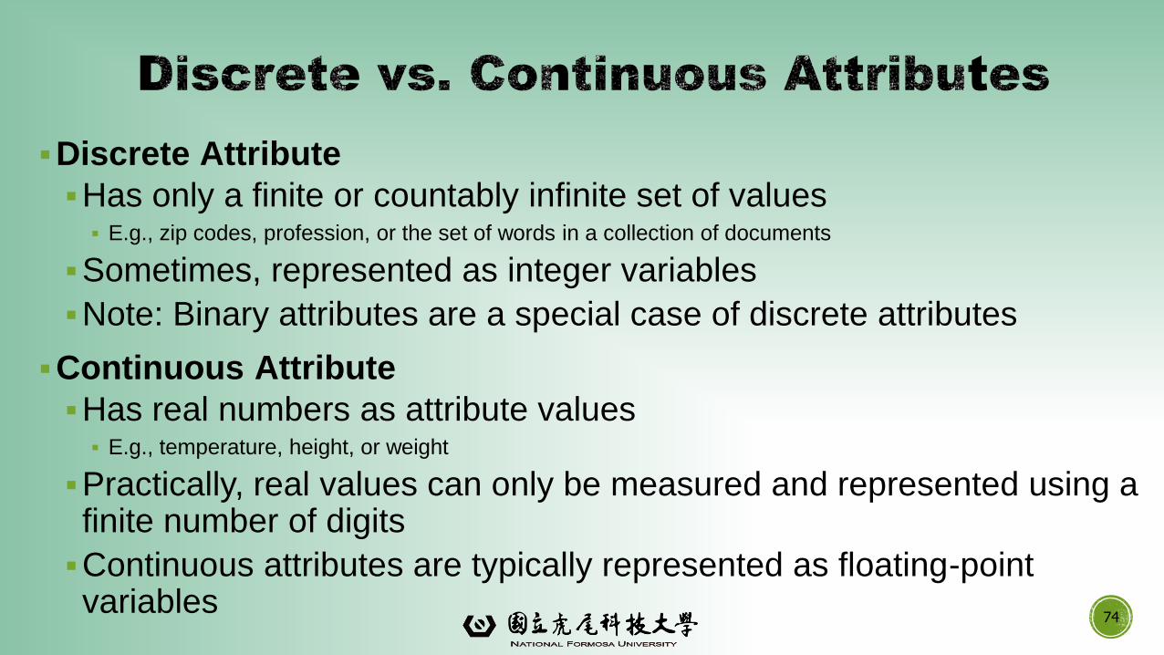
▪Discrete Attribute
▪Has only a finite or countably infinite set of values▪ E.g., zip codes, profession, or the set of words in a collection of documents
▪Sometimes, represented as integer variables
▪Note: Binary attributes are a special case of discrete attributes
▪Continuous Attribute
▪Has real numbers as attribute values▪ E.g., temperature, height, or weight
▪Practically, real values can only be measured and represented using a finite number of digits
▪Continuous attributes are typically represented as floating-point variables
74
Data Objects and Attribute Types
Basic Statistical Descriptions of Data
Data Visualization
Measuring Data Similarity and Dissimilarity
Summary
75
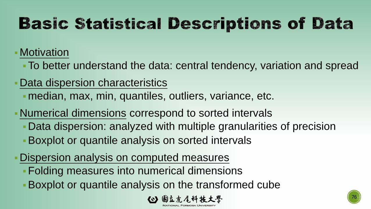
▪Motivation
▪To better understand the data: central tendency, variation and spread
▪Data dispersion characteristics
▪median, max, min, quantiles, outliers, variance, etc.
▪Numerical dimensions correspond to sorted intervals
▪Data dispersion: analyzed with multiple granularities of precision
▪Boxplot or quantile analysis on sorted intervals
▪Dispersion analysis on computed measures
▪Folding measures into numerical dimensions
▪Boxplot or quantile analysis on the transformed cube76
Measuring the Central Tendency
▪ Mean (algebraic measure) (sample vs. population):
Note: n is sample size and N is population size.
▪ Weighted arithmetic mean:
▪ Trimmed mean: chopping extreme values
▪ Median:
▪ Middle value if odd number of values, or average of the middle two values
otherwise
▪ Estimated by interpolation (for grouped data):
▪ Mode
▪ Value that occurs most frequently in the data
▪ Unimodal, bimodal, trimodal
▪ Empirical formula:
N
x
77
n
i
ixn
x1
1
n
i
i
n
i
ii
w
xw
x
1
1
widthfreq
lfreqnLmedian
median
))(2/
(1
)(3 medianmeanmodemean
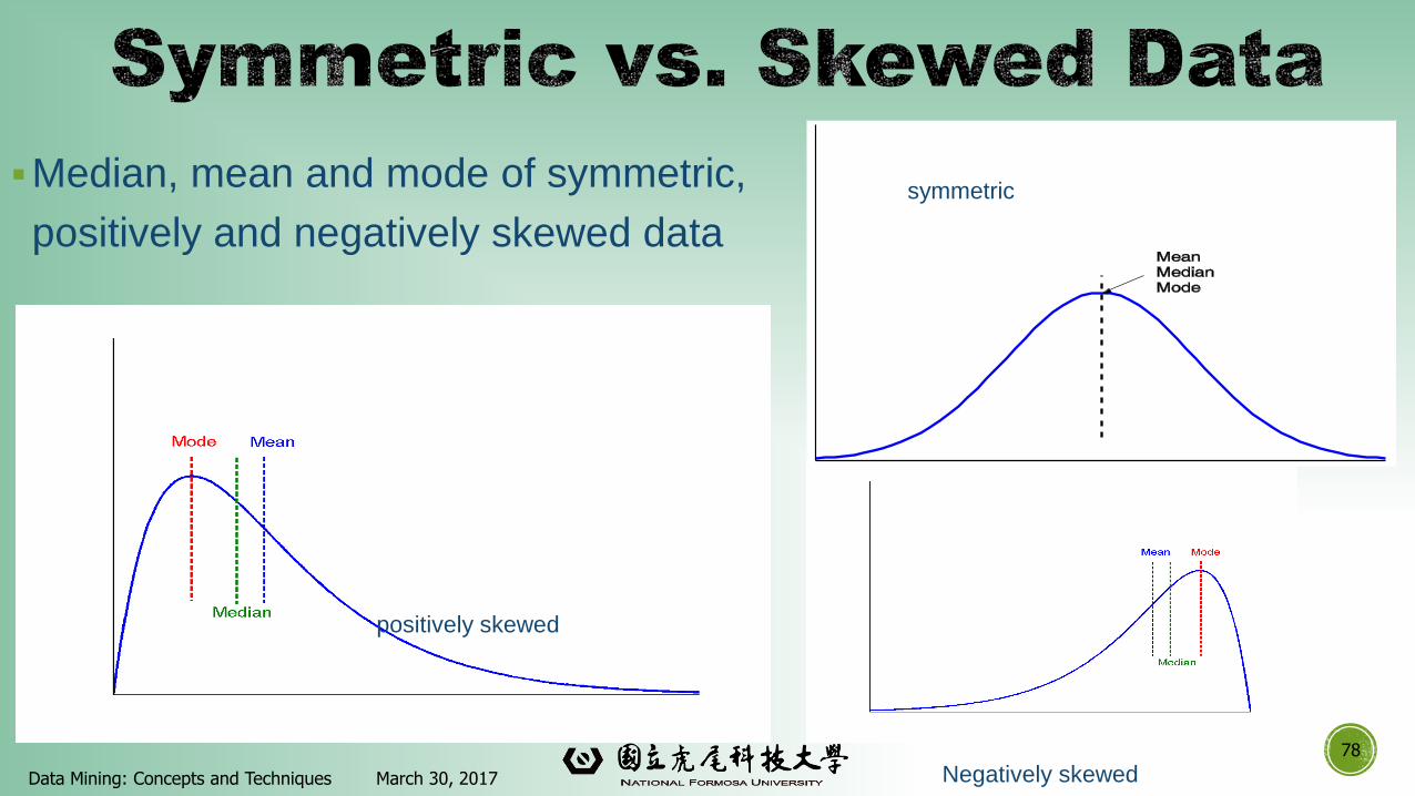
▪Median, mean and mode of symmetric,
positively and negatively skewed data
78
March 30, 2017Data Mining: Concepts and Techniques
positively skewed
Negatively skewed
symmetric
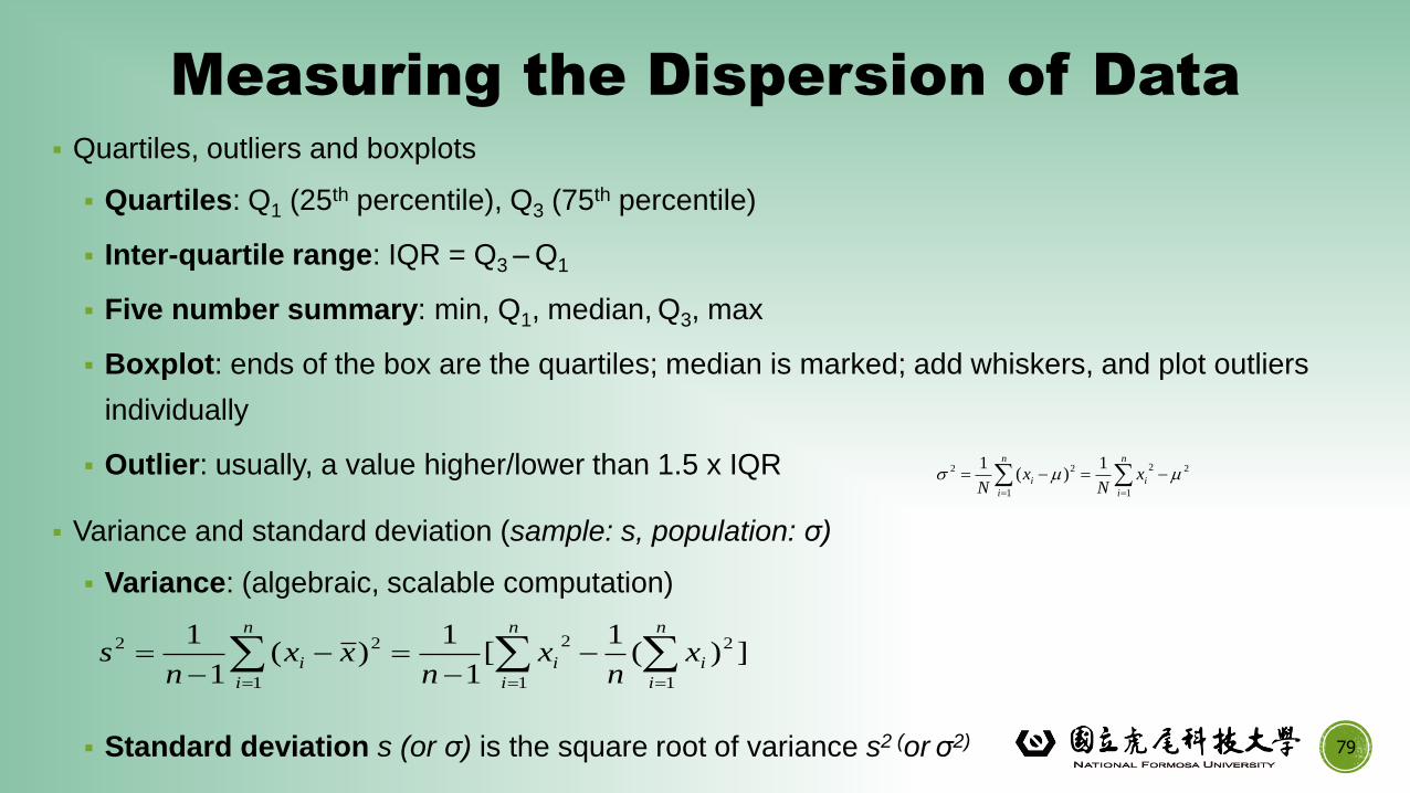
Measuring the Dispersion of Data
▪ Quartiles, outliers and boxplots
▪ Quartiles: Q1 (25th percentile), Q3 (75th percentile)
▪ Inter-quartile range: IQR = Q3 – Q1
▪ Five number summary: min, Q1, median, Q3, max
▪ Boxplot: ends of the box are the quartiles; median is marked; add whiskers, and plot outliers
individually
▪ Outlier: usually, a value higher/lower than 1.5 x IQR
▪ Variance and standard deviation (sample: s, population: σ)
▪ Variance: (algebraic, scalable computation)
▪ Standard deviation s (or σ) is the square root of variance s2 (or σ2)
n
i
i
n
i
i xN
xN 1
22
1
22 1)(
1
79
n
i
n
i
ii
n
i
i xn
xn
xxn
s1 1
22
1
22 ])(1
[1
1)(
1
1
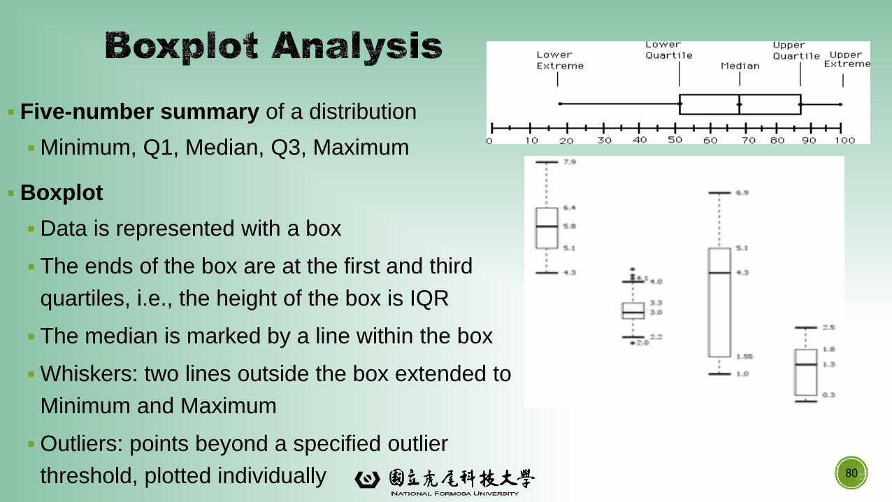
▪ Five-number summary of a distribution
▪Minimum, Q1, Median, Q3, Maximum
▪Boxplot
▪Data is represented with a box
▪ The ends of the box are at the first and third
quartiles, i.e., the height of the box is IQR
▪ The median is marked by a line within the box
▪Whiskers: two lines outside the box extended to
Minimum and Maximum
▪Outliers: points beyond a specified outlier
threshold, plotted individually 80
March 30, 2017 Data Mining: Concepts and Techniques
81
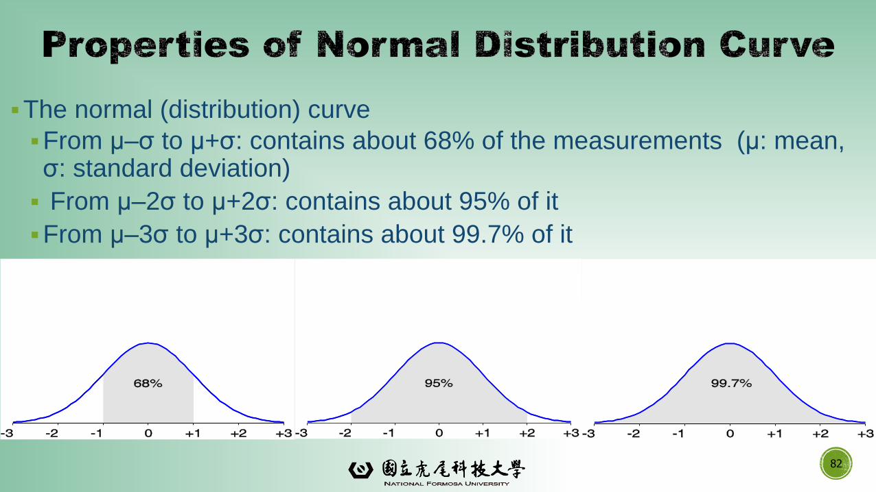
▪The normal (distribution) curve
▪From μ–σ to μ+σ: contains about 68% of the measurements (μ: mean, σ: standard deviation)
▪ From μ–2σ to μ+2σ: contains about 95% of it
▪From μ–3σ to μ+3σ: contains about 99.7% of it
82
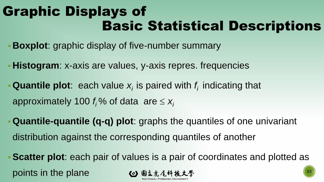
Graphic Displays of
Basic Statistical Descriptions
▪Boxplot: graphic display of five-number summary
▪Histogram: x-axis are values, y-axis repres. frequencies
▪Quantile plot: each value xi is paired with fi indicating that
approximately 100 fi % of data are xi
▪Quantile-quantile (q-q) plot: graphs the quantiles of one univariant
distribution against the corresponding quantiles of another
▪Scatter plot: each pair of values is a pair of coordinates and plotted as
points in the plane 83
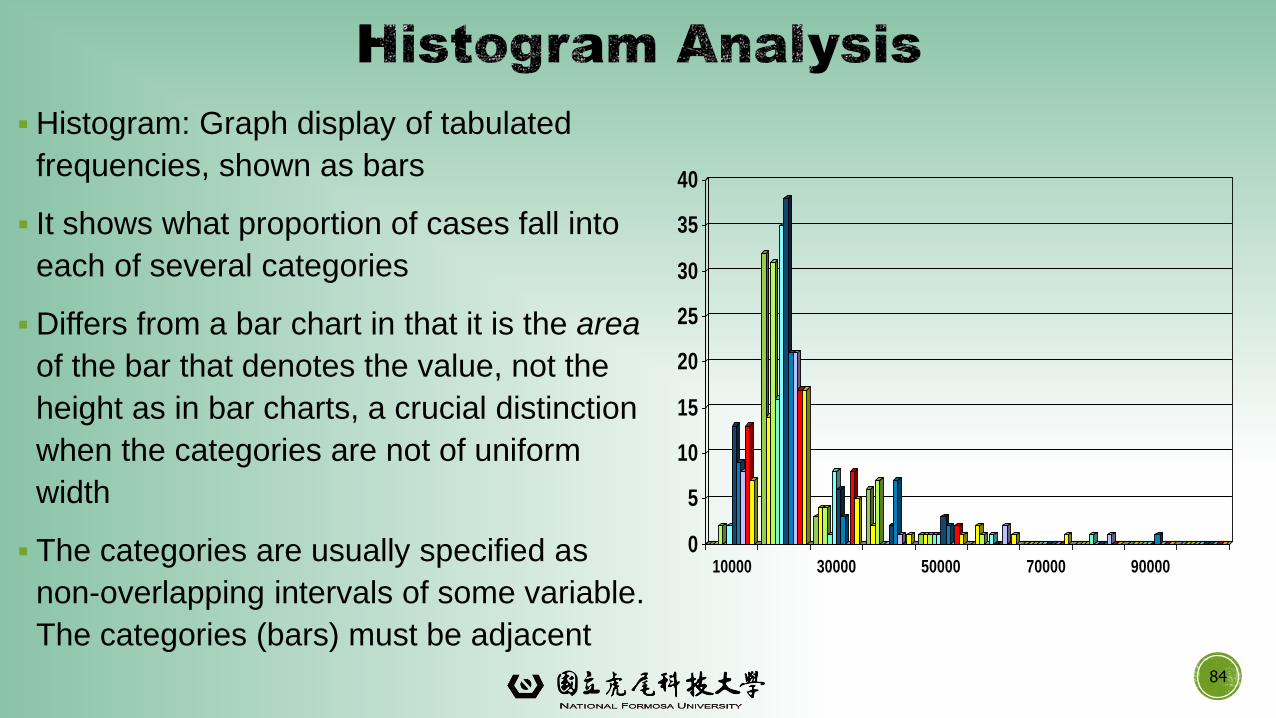
▪Histogram: Graph display of tabulated
frequencies, shown as bars
▪ It shows what proportion of cases fall into
each of several categories
▪Differs from a bar chart in that it is the area
of the bar that denotes the value, not the
height as in bar charts, a crucial distinction
when the categories are not of uniform
width
▪ The categories are usually specified as
non-overlapping intervals of some variable.
The categories (bars) must be adjacent
0
5
10
15
20
25
30
35
40
10000 30000 50000 70000 90000
84
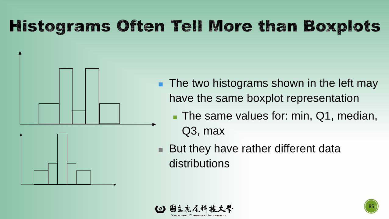
85
The two histograms shown in the left may
have the same boxplot representation
The same values for: min, Q1, median,
Q3, max
But they have rather different data
distributions
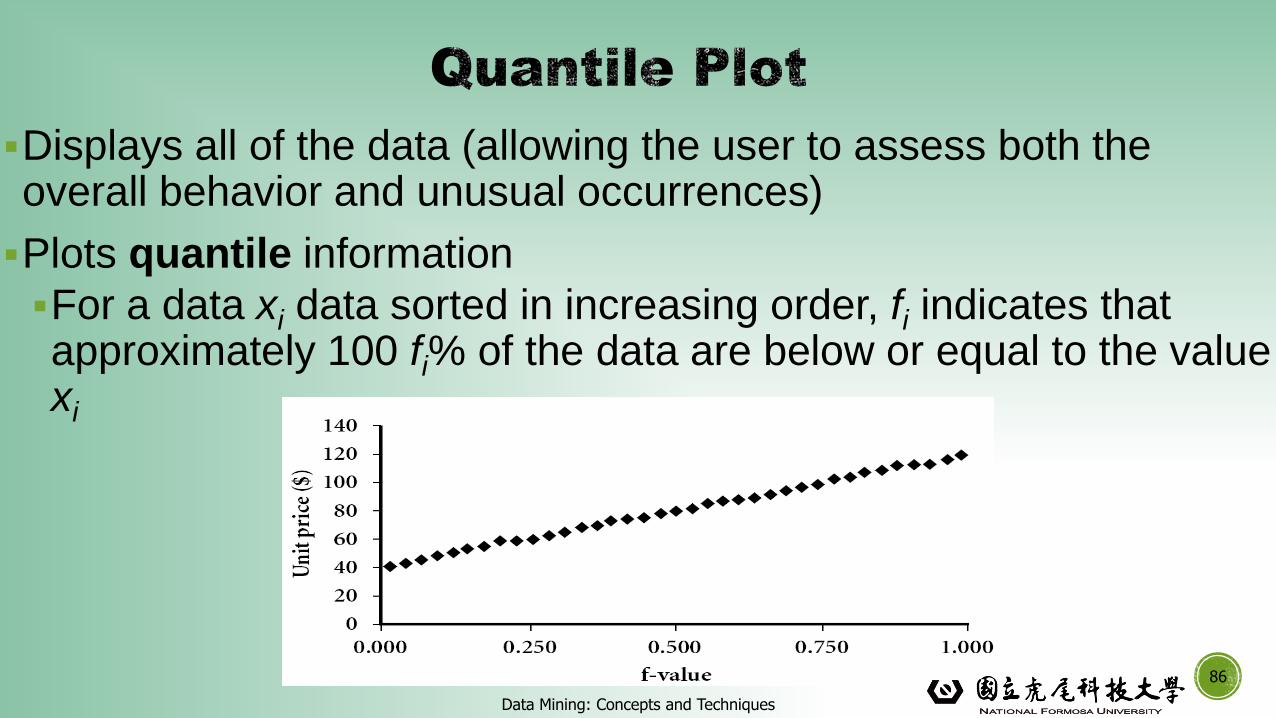
▪Displays all of the data (allowing the user to assess both the overall behavior and unusual occurrences)
▪Plots quantile information
▪For a data xi data sorted in increasing order, fi indicates that approximately 100 fi% of the data are below or equal to the value xi
Data Mining: Concepts and Techniques
86
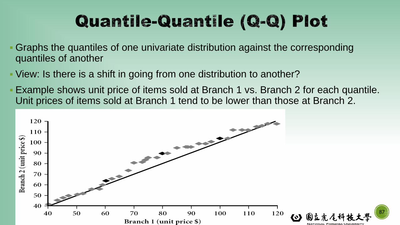
▪Graphs the quantiles of one univariate distribution against the corresponding quantiles of another
▪ View: Is there is a shift in going from one distribution to another?
▪ Example shows unit price of items sold at Branch 1 vs. Branch 2 for each quantile. Unit prices of items sold at Branch 1 tend to be lower than those at Branch 2.
87
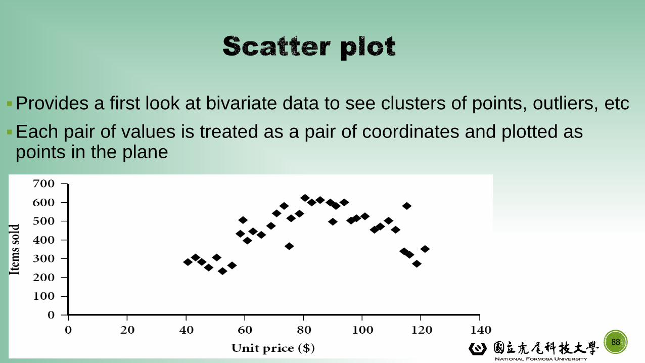
▪Provides a first look at bivariate data to see clusters of points, outliers, etc
▪Each pair of values is treated as a pair of coordinates and plotted as points in the plane
88
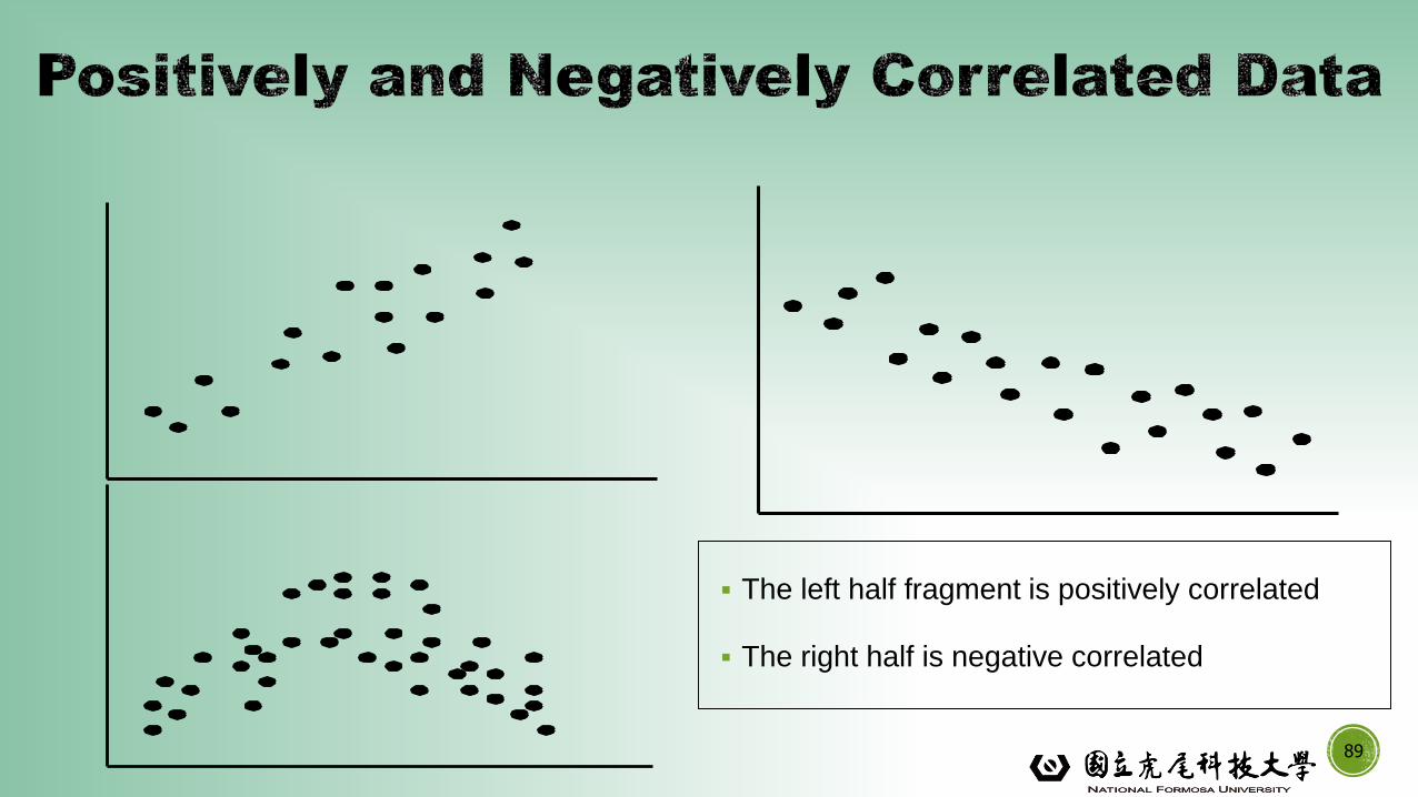
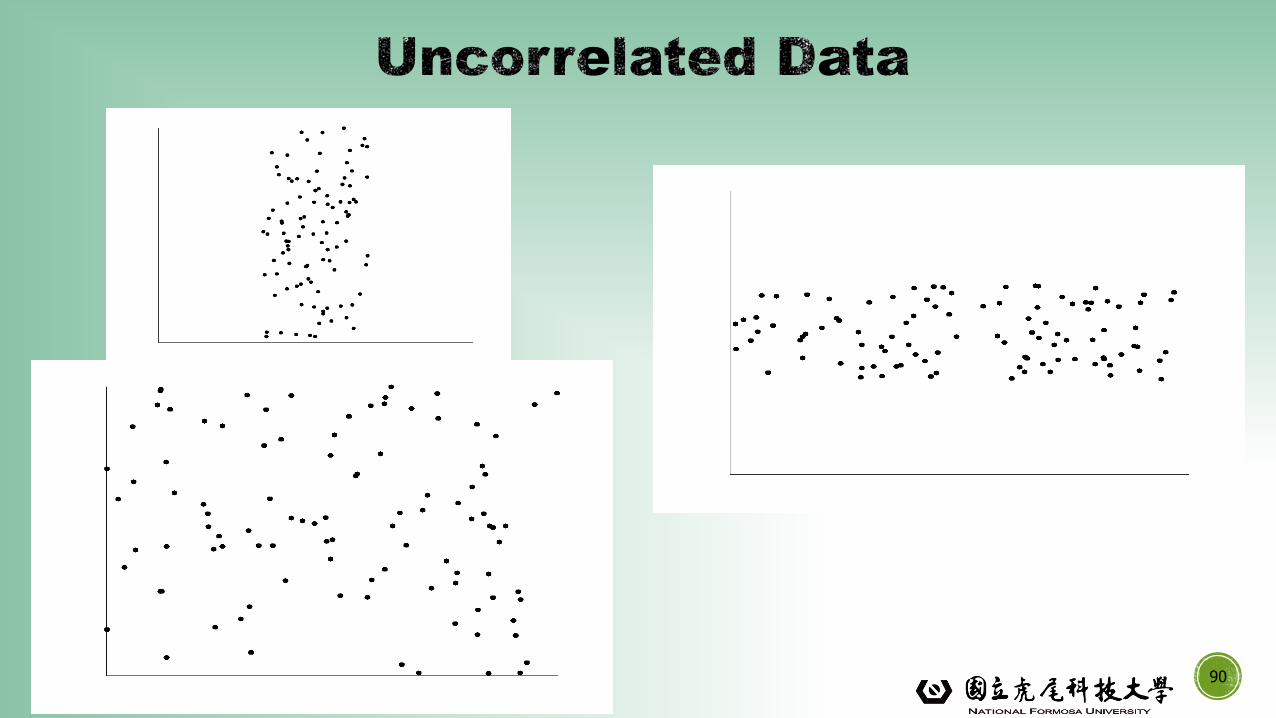
▪ The left half fragment is positively correlated
▪ The right half is negative correlated
89
90
Data Objects and Attribute Types
Basic Statistical Descriptions of Data
Data Visualization
Measuring Data Similarity and Dissimilarity
Summary
91
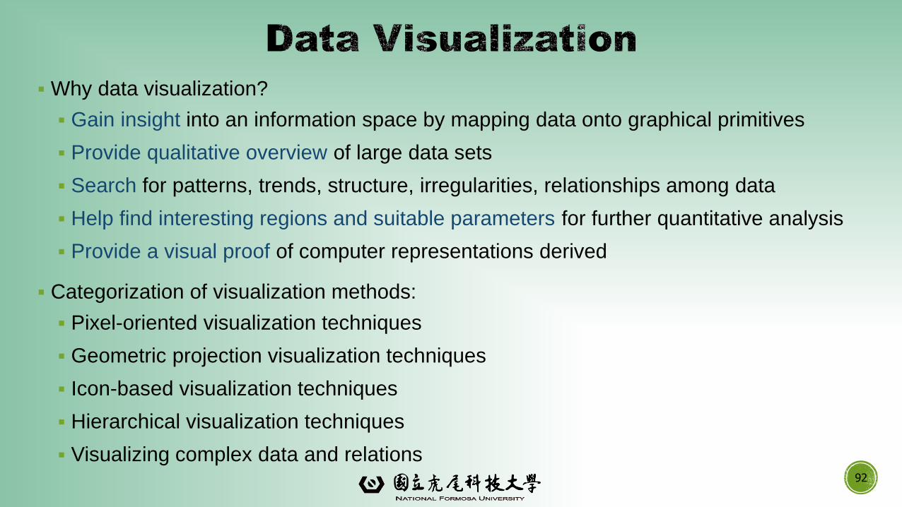
▪ Why data visualization?
▪ Gain insight into an information space by mapping data onto graphical primitives
▪ Provide qualitative overview of large data sets
▪ Search for patterns, trends, structure, irregularities, relationships among data
▪ Help find interesting regions and suitable parameters for further quantitative analysis
▪ Provide a visual proof of computer representations derived
▪ Categorization of visualization methods:
▪ Pixel-oriented visualization techniques
▪ Geometric projection visualization techniques
▪ Icon-based visualization techniques
▪ Hierarchical visualization techniques
▪ Visualizing complex data and relations92
93
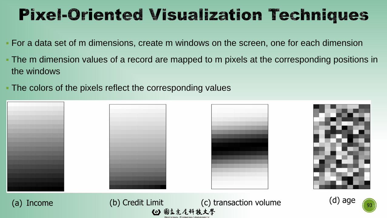
▪ For a data set of m dimensions, create m windows on the screen, one for each dimension
▪ The m dimension values of a record are mapped to m pixels at the corresponding positions in
the windows
▪ The colors of the pixels reflect the corresponding values
(a) Income (b) Credit Limit (c) transaction volume (d) age
94
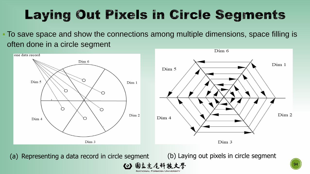
▪ To save space and show the connections among multiple dimensions, space filling is
often done in a circle segment
(a) Representing a data record in circle segment (b) Laying out pixels in circle segment
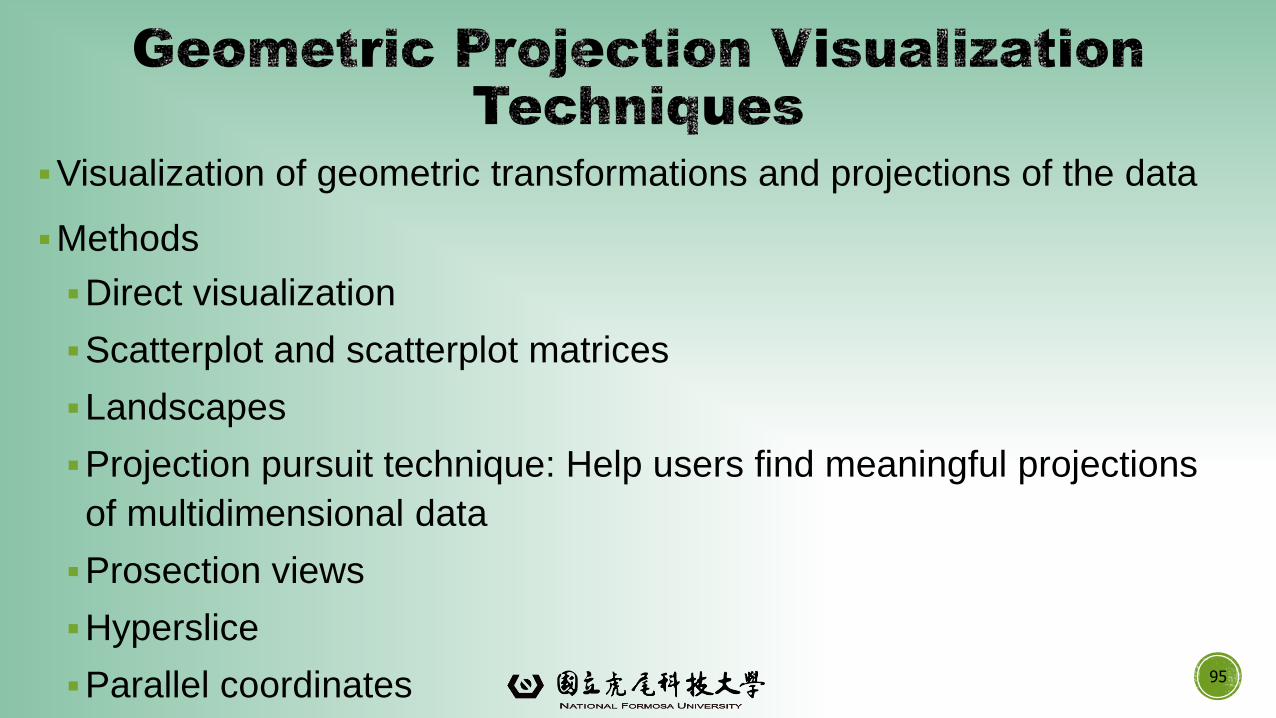
▪Visualization of geometric transformations and projections of the data
▪Methods
▪Direct visualization
▪Scatterplot and scatterplot matrices
▪Landscapes
▪Projection pursuit technique: Help users find meaningful projections
of multidimensional data
▪Prosection views
▪Hyperslice
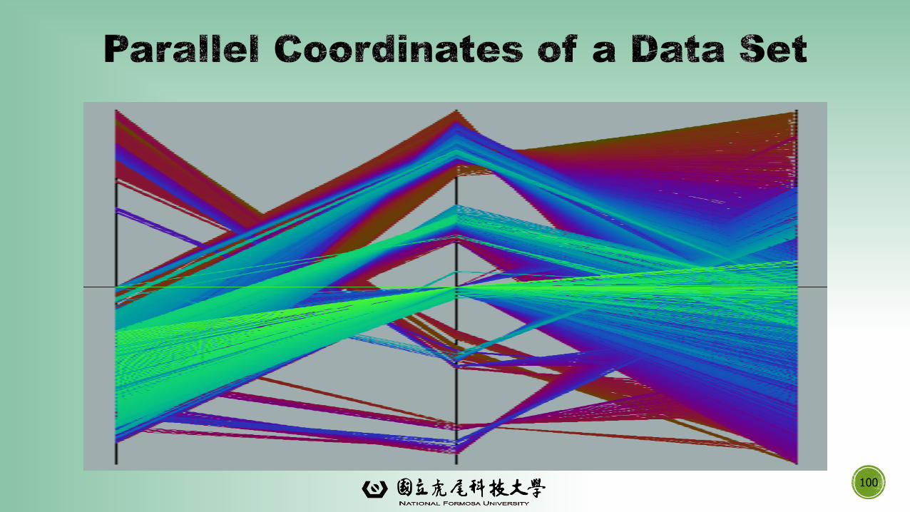
▪Parallel coordinates 95
Data Mining: Concepts and Techniques
96
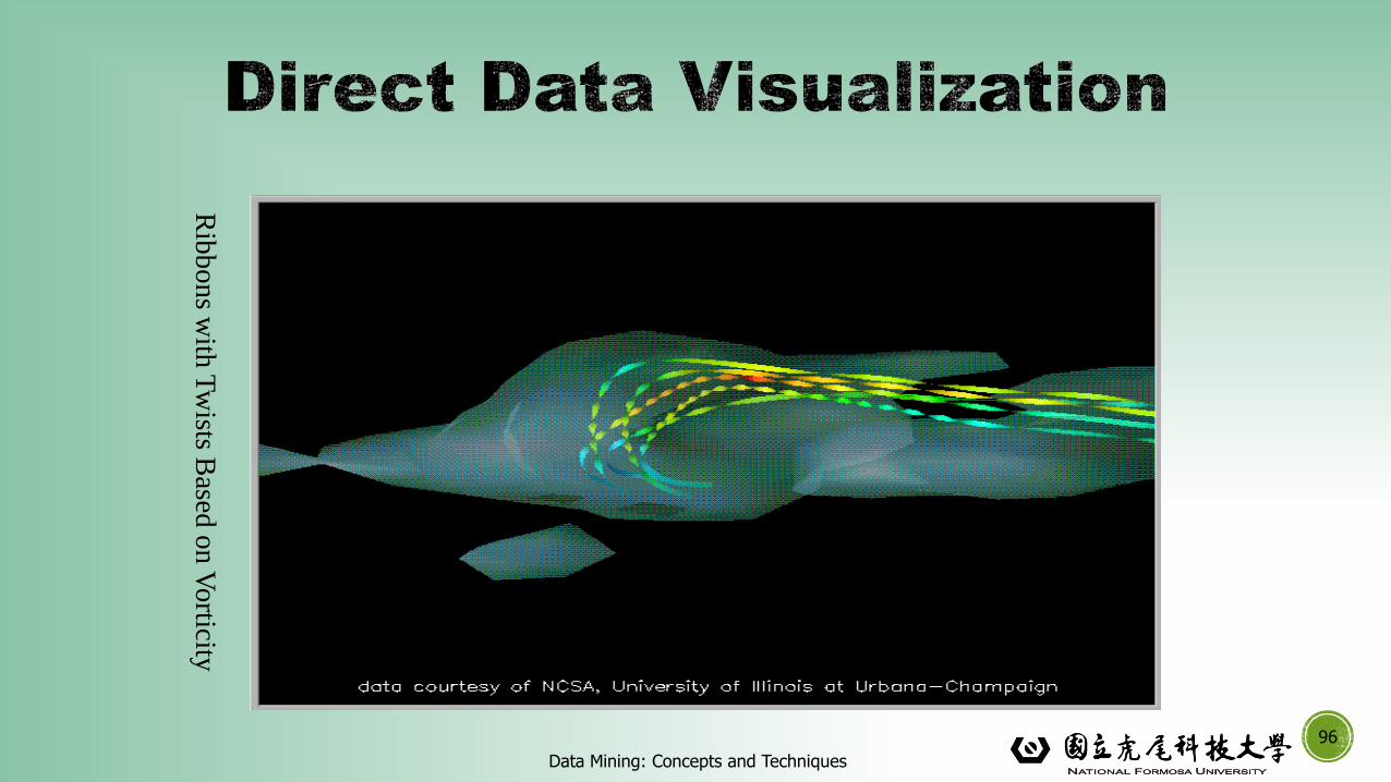
Rib
bon
s with
Tw
ists Based
on
Vo
rticity
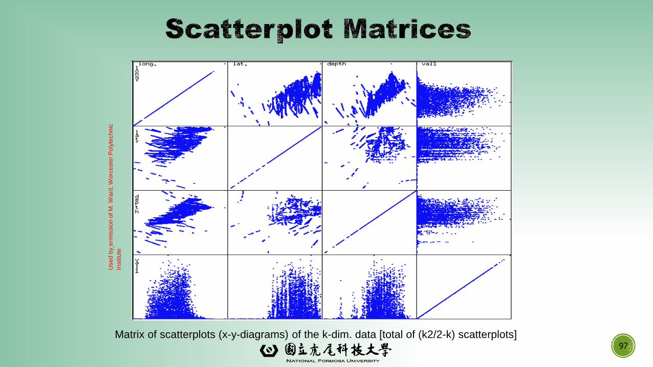
Matrix of scatterplots (x-y-diagrams) of the k-dim. data [total of (k2/2-k) scatterplots]97
Use
d b
ye
rmis
sio
n o
f M
. W
ard
, W
orc
este
r P
oly
tech
nic
Institu
te
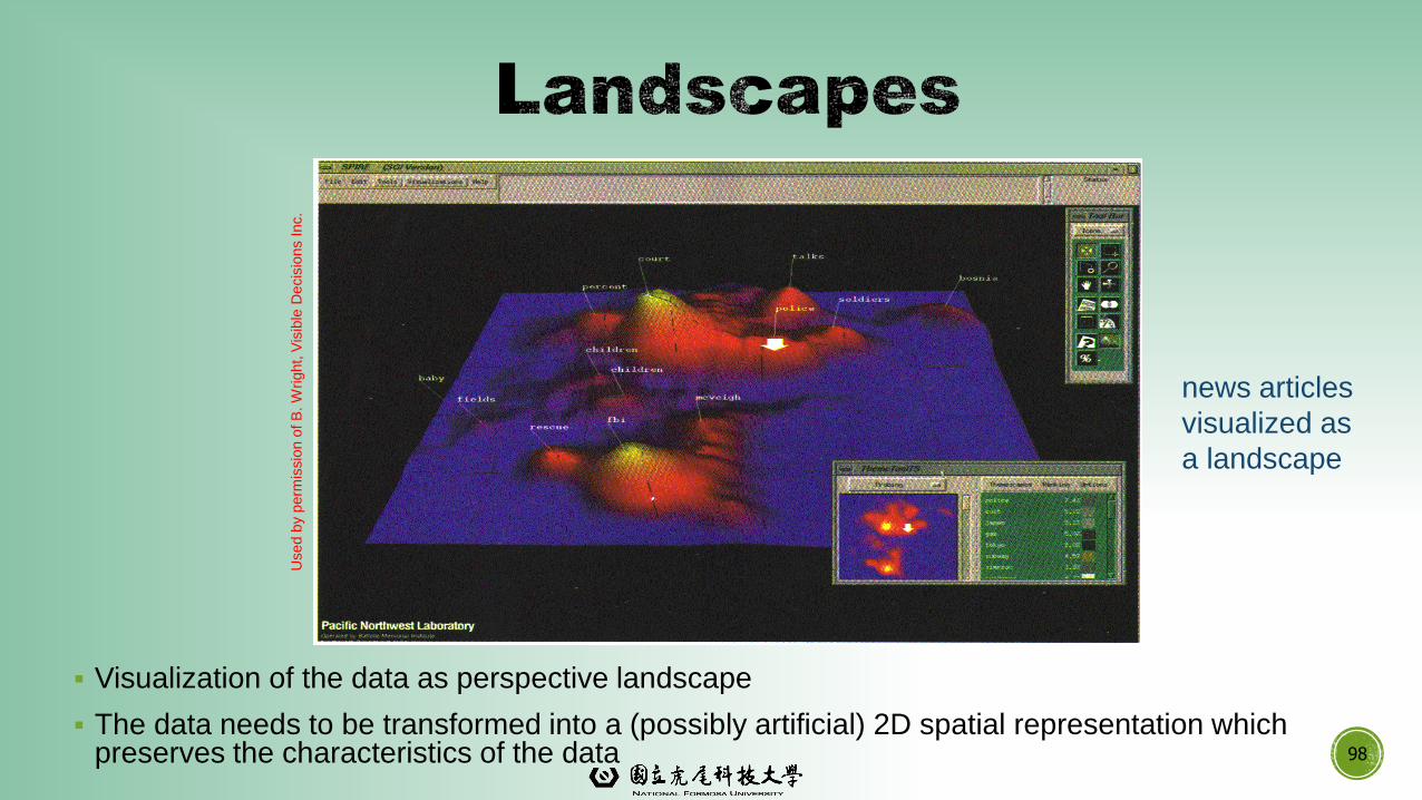
▪ Visualization of the data as perspective landscape
▪ The data needs to be transformed into a (possibly artificial) 2D spatial representation which preserves the characteristics of the data 98
news articles
visualized as
a landscape
Used b
y perm
issio
n o
f B
. W
right, V
isib
le D
ecis
ions Inc.
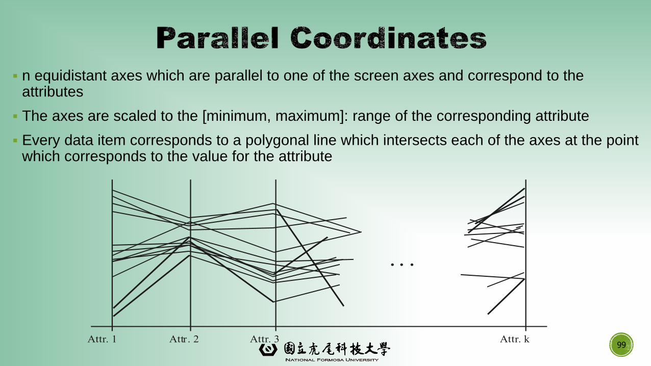
▪ n equidistant axes which are parallel to one of the screen axes and correspond to the attributes
▪ The axes are scaled to the [minimum, maximum]: range of the corresponding attribute
▪ Every data item corresponds to a polygonal line which intersects each of the axes at the point which corresponds to the value for the attribute
99Attr. 1 Attr. 2 Attr. kAttr. 3
• • •
100
Icon-Based Visualization Techniques
▪Visualization of the data values as features of icons
▪Typical visualization methods
▪Chernoff Faces
▪Stick Figures
▪General techniques
▪Shape coding: Use shape to represent certain information encoding
▪Color icons: Use color icons to encode more information
▪Tile bars: Use small icons to represent the relevant feature vectors in
document retrieval101
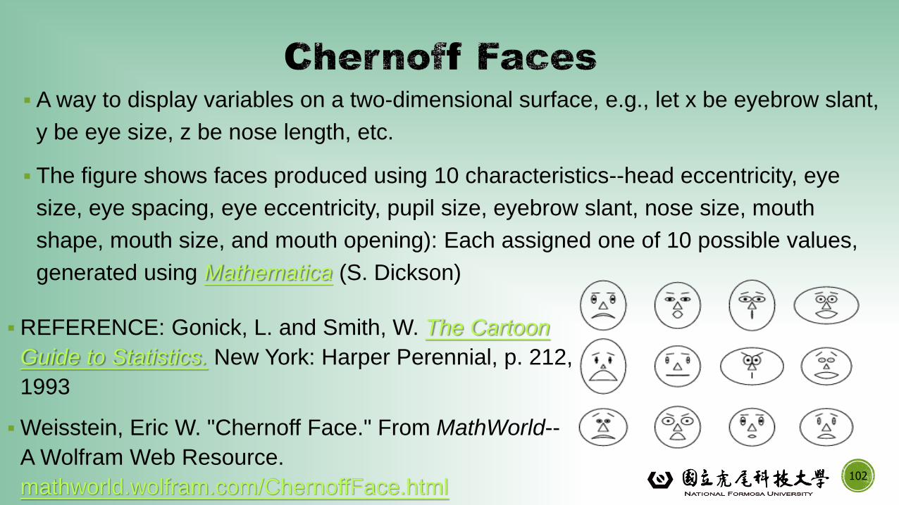
▪ A way to display variables on a two-dimensional surface, e.g., let x be eyebrow slant,
y be eye size, z be nose length, etc.
▪ The figure shows faces produced using 10 characteristics--head eccentricity, eye
size, eye spacing, eye eccentricity, pupil size, eyebrow slant, nose size, mouth
shape, mouth size, and mouth opening): Each assigned one of 10 possible values,
generated using Mathematica (S. Dickson)
▪REFERENCE: Gonick, L. and Smith, W. The Cartoon
Guide to Statistics. New York: Harper Perennial, p. 212,
1993
▪Weisstein, Eric W. "Chernoff Face." From MathWorld--
A Wolfram Web Resource.
mathworld.wolfram.com/ChernoffFace.html102
103
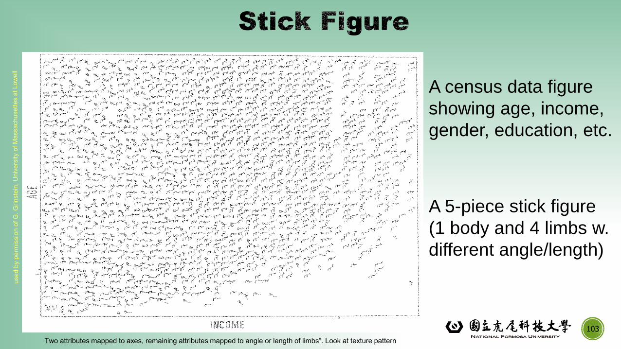
Two attributes mapped to axes, remaining attributes mapped to angle or length of limbs”. Look at texture pattern
A census data figure
showing age, income,
gender, education, etc.
A 5-piece stick figure
(1 body and 4 limbs w.
different angle/length)
Hierarchical Visualization Techniques
▪Visualization of the data using a hierarchical partitioning into subspaces
▪Methods
▪Dimensional Stacking
▪Worlds-within-Worlds
▪ Tree-Map
▪Cone Trees
▪ InfoCube
104
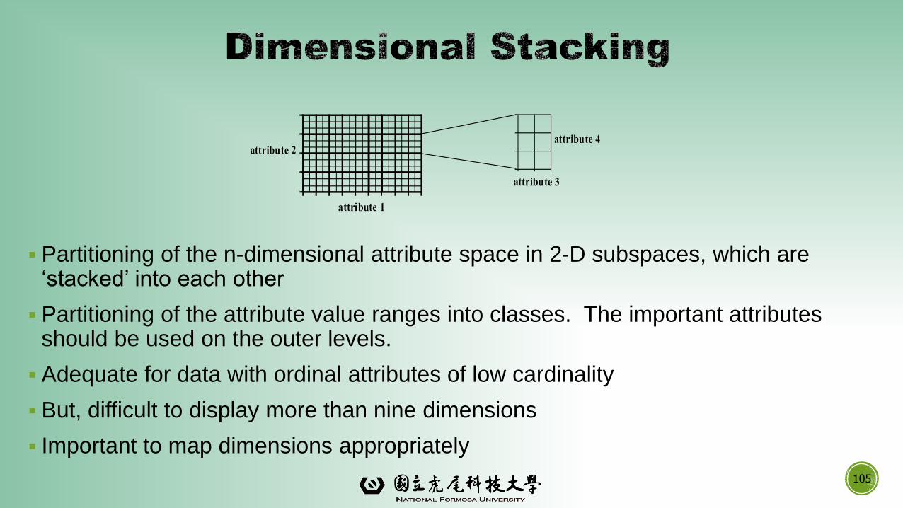
attribute 1
attribute 2
attribute 3
attribute 4
▪ Partitioning of the n-dimensional attribute space in 2-D subspaces, which are ‘stacked’ into each other
▪ Partitioning of the attribute value ranges into classes. The important attributes should be used on the outer levels.
▪ Adequate for data with ordinal attributes of low cardinality
▪ But, difficult to display more than nine dimensions
▪ Important to map dimensions appropriately
105
106
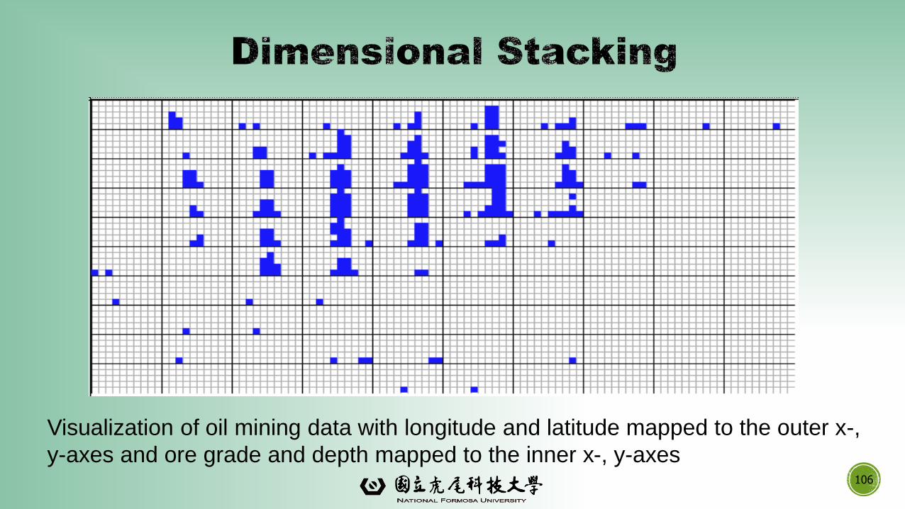
Visualization of oil mining data with longitude and latitude mapped to the outer x-,
y-axes and ore grade and depth mapped to the inner x-, y-axes
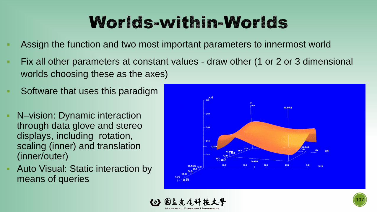
▪ Assign the function and two most important parameters to innermost world
▪ Fix all other parameters at constant values - draw other (1 or 2 or 3 dimensional
worlds choosing these as the axes)
▪ Software that uses this paradigm
▪ N–vision: Dynamic interaction through data glove and stereo displays, including rotation, scaling (inner) and translation (inner/outer)
▪ Auto Visual: Static interaction by means of queries
107
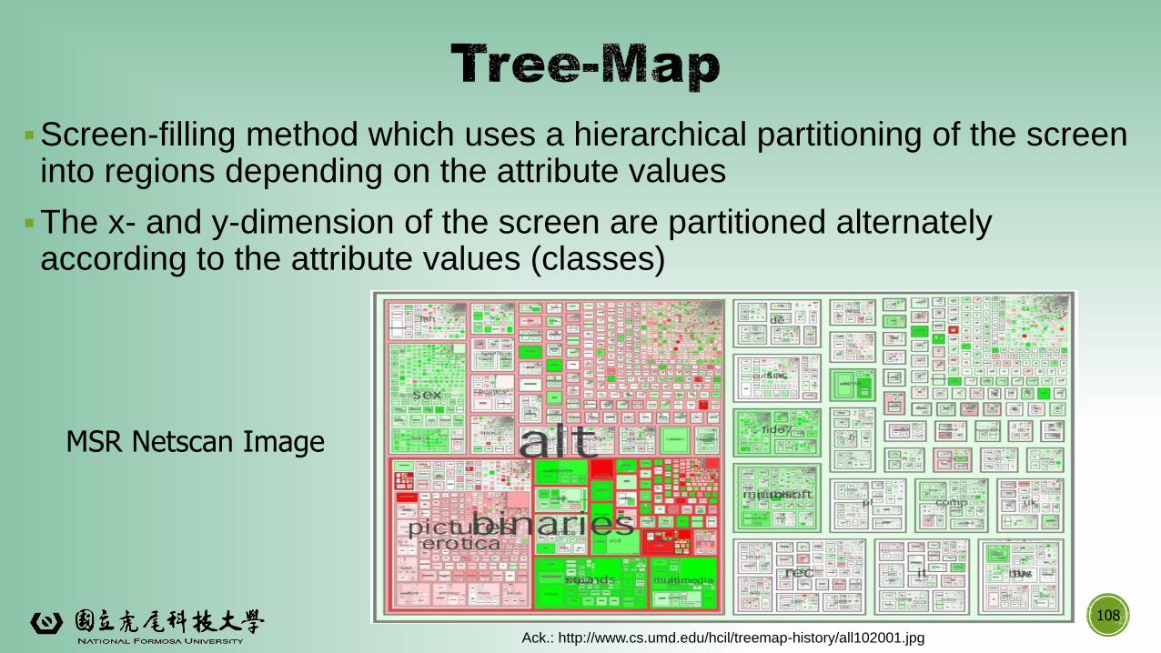
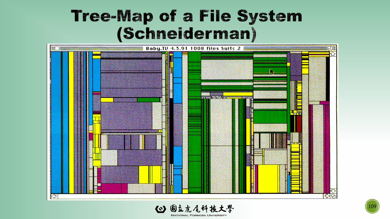
▪Screen-filling method which uses a hierarchical partitioning of the screen into regions depending on the attribute values
▪The x- and y-dimension of the screen are partitioned alternately according to the attribute values (classes)
108
MSR Netscan Image
Ack.: http://www.cs.umd.edu/hcil/treemap-history/all102001.jpg
109
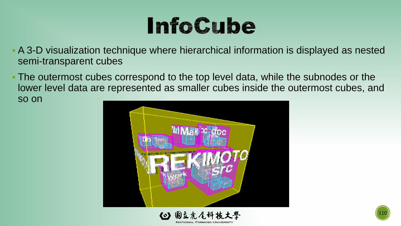
▪ A 3-D visualization technique where hierarchical information is displayed as nested semi-transparent cubes
▪ The outermost cubes correspond to the top level data, while the subnodes or the lower level data are represented as smaller cubes inside the outermost cubes, and so on
110
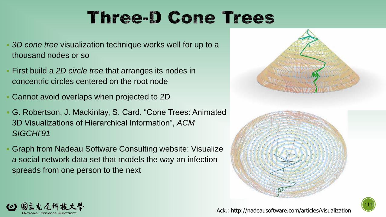
▪ 3D cone tree visualization technique works well for up to a
thousand nodes or so
▪ First build a 2D circle tree that arranges its nodes in
concentric circles centered on the root node
▪ Cannot avoid overlaps when projected to 2D
▪ G. Robertson, J. Mackinlay, S. Card. “Cone Trees: Animated
3D Visualizations of Hierarchical Information”, ACM
SIGCHI'91
▪ Graph from Nadeau Software Consulting website: Visualize
a social network data set that models the way an infection
spreads from one person to the next
111
Ack.: http://nadeausoftware.com/articles/visualization
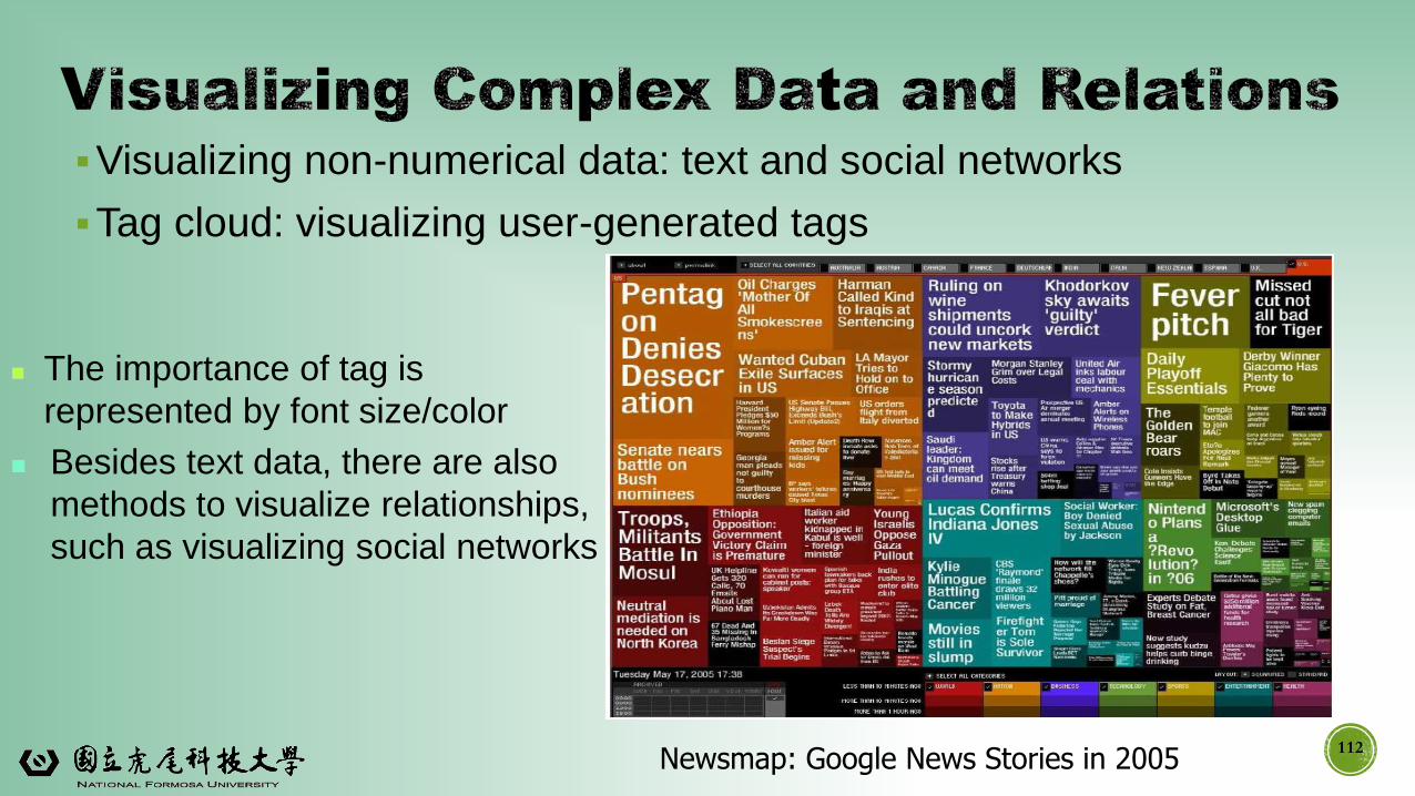
▪Visualizing non-numerical data: text and social networks
▪Tag cloud: visualizing user-generated tags
The importance of tag is
represented by font size/color
Besides text data, there are also
methods to visualize relationships,
such as visualizing social networks
Newsmap: Google News Stories in 2005112
Data Objects and Attribute Types
Basic Statistical Descriptions of Data
Data Visualization
Measuring Data Similarity and Dissimilarity
Summary
113
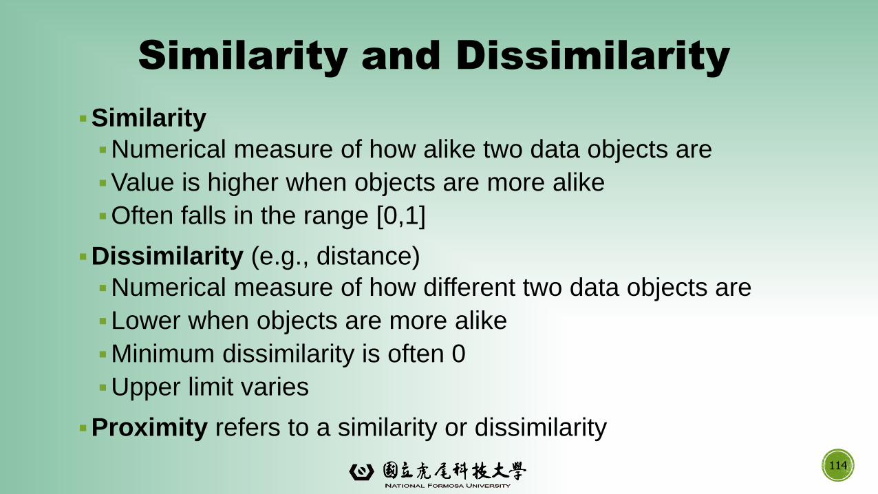
Similarity and Dissimilarity
▪Similarity
▪Numerical measure of how alike two data objects are
▪Value is higher when objects are more alike
▪Often falls in the range [0,1]
▪Dissimilarity (e.g., distance)
▪Numerical measure of how different two data objects are
▪Lower when objects are more alike
▪Minimum dissimilarity is often 0
▪Upper limit varies
▪Proximity refers to a similarity or dissimilarity
114
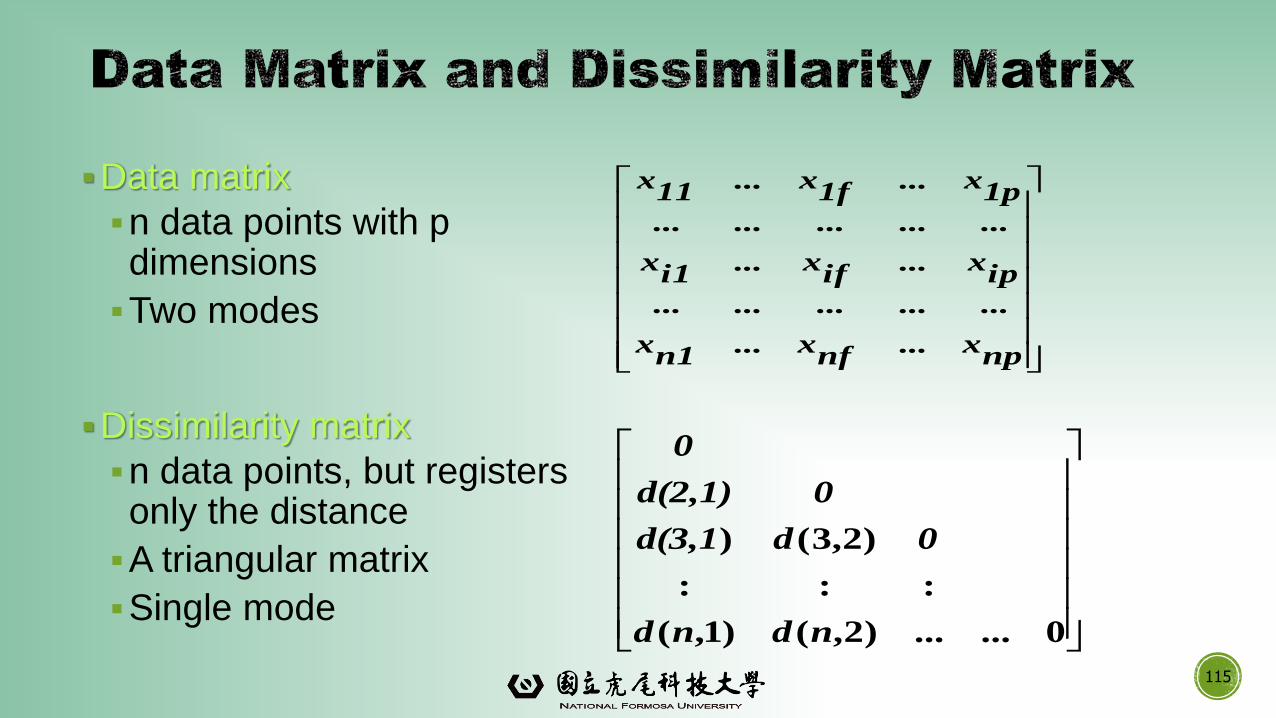
▪Data matrix
▪n data points with p dimensions
▪Two modes
▪Dissimilarity matrix
▪n data points, but registers only the distance
▪A triangular matrix
▪Single mode
115
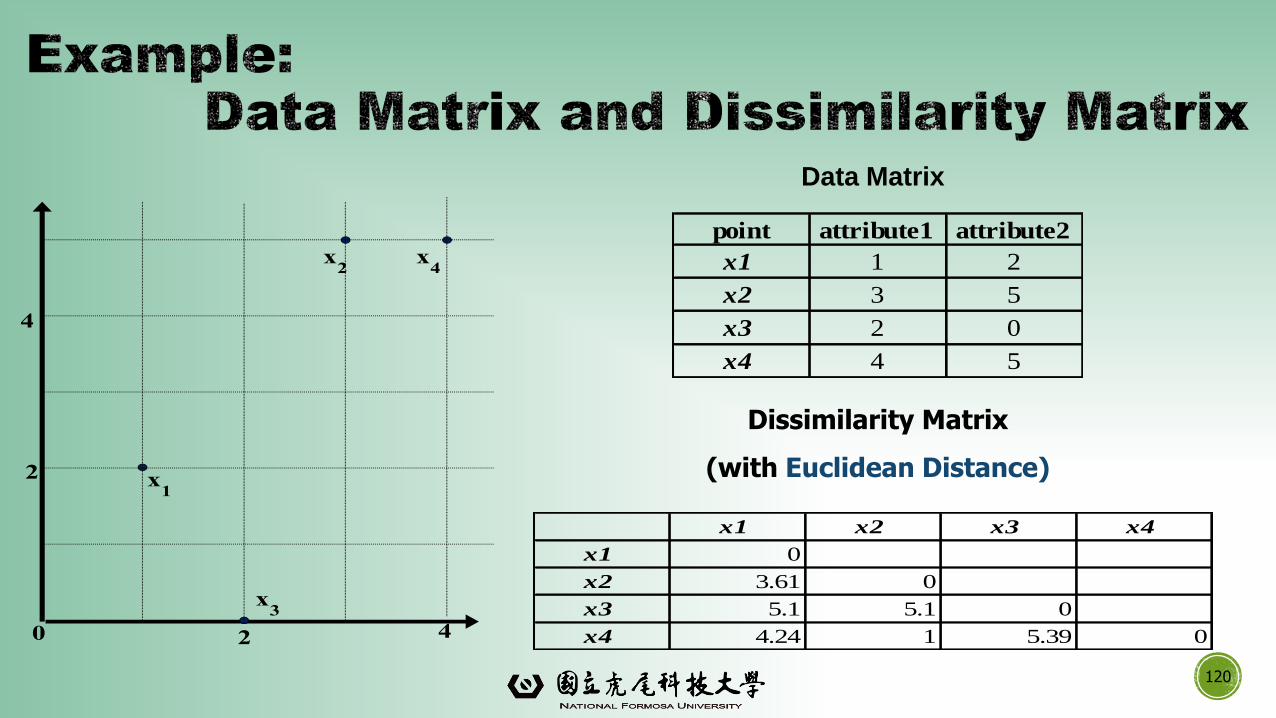
npx...nfx...n1x
...............
ipx...ifx...i1x
...............
1px...1fx...11x
0...)2,()1,(
:::
)2,3()
...ndnd
0dd(3,1
0d(2,1)
0
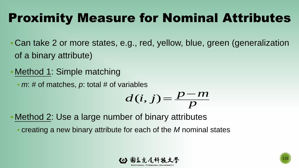
Proximity Measure for Nominal Attributes
▪Can take 2 or more states, e.g., red, yellow, blue, green (generalization
of a binary attribute)
▪Method 1: Simple matching
▪m: # of matches, p: total # of variables
▪Method 2: Use a large number of binary attributes
▪ creating a new binary attribute for each of the M nominal states
116
pmp
jid
),(
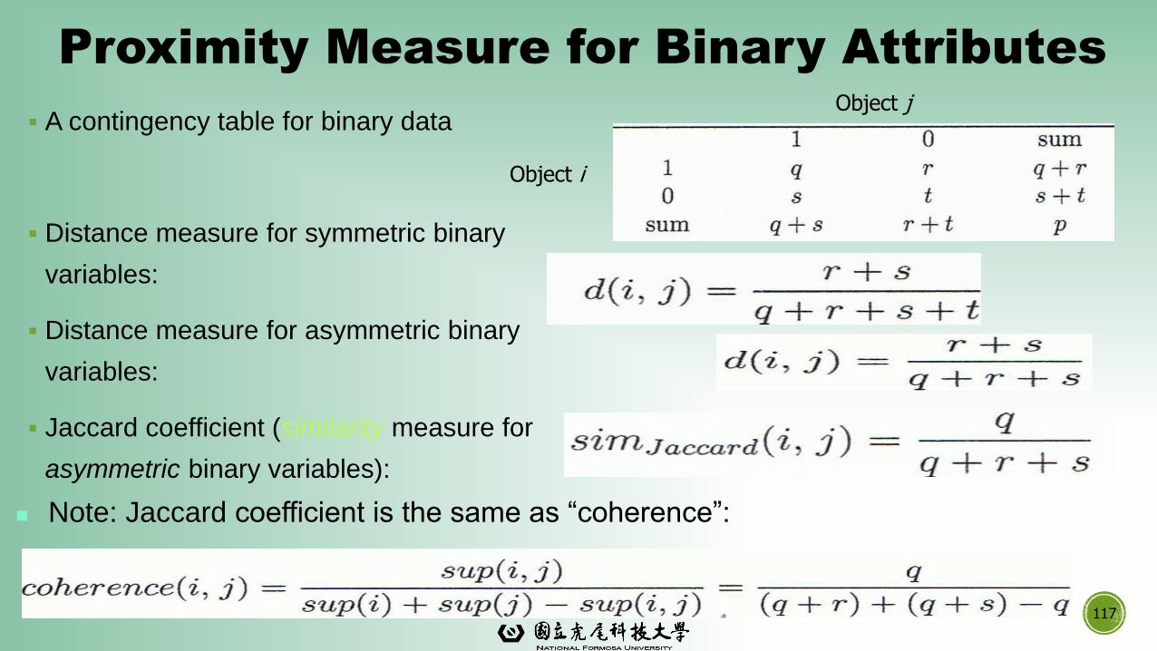
Proximity Measure for Binary Attributes
▪ A contingency table for binary data
▪ Distance measure for symmetric binary
variables:
▪ Distance measure for asymmetric binary
variables:
▪ Jaccard coefficient (similarity measure for
asymmetric binary variables):
117
Note: Jaccard coefficient is the same as “coherence”:
Object i
Object j
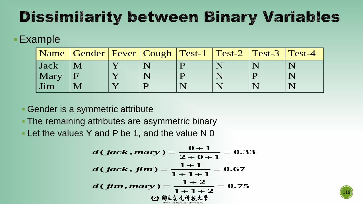
▪Example
▪Gender is a symmetric attribute
▪ The remaining attributes are asymmetric binary
▪ Let the values Y and P be 1, and the value N 0
118
Name Gender Fever Cough Test-1 Test-2 Test-3 Test-4
Jack M Y N P N N N
Mary F Y N P N P N
Jim M Y P N N N N
75.0211
21),(
67.0111
11),(
33.0102
10),(
maryjimd
jimjackd
maryjackd
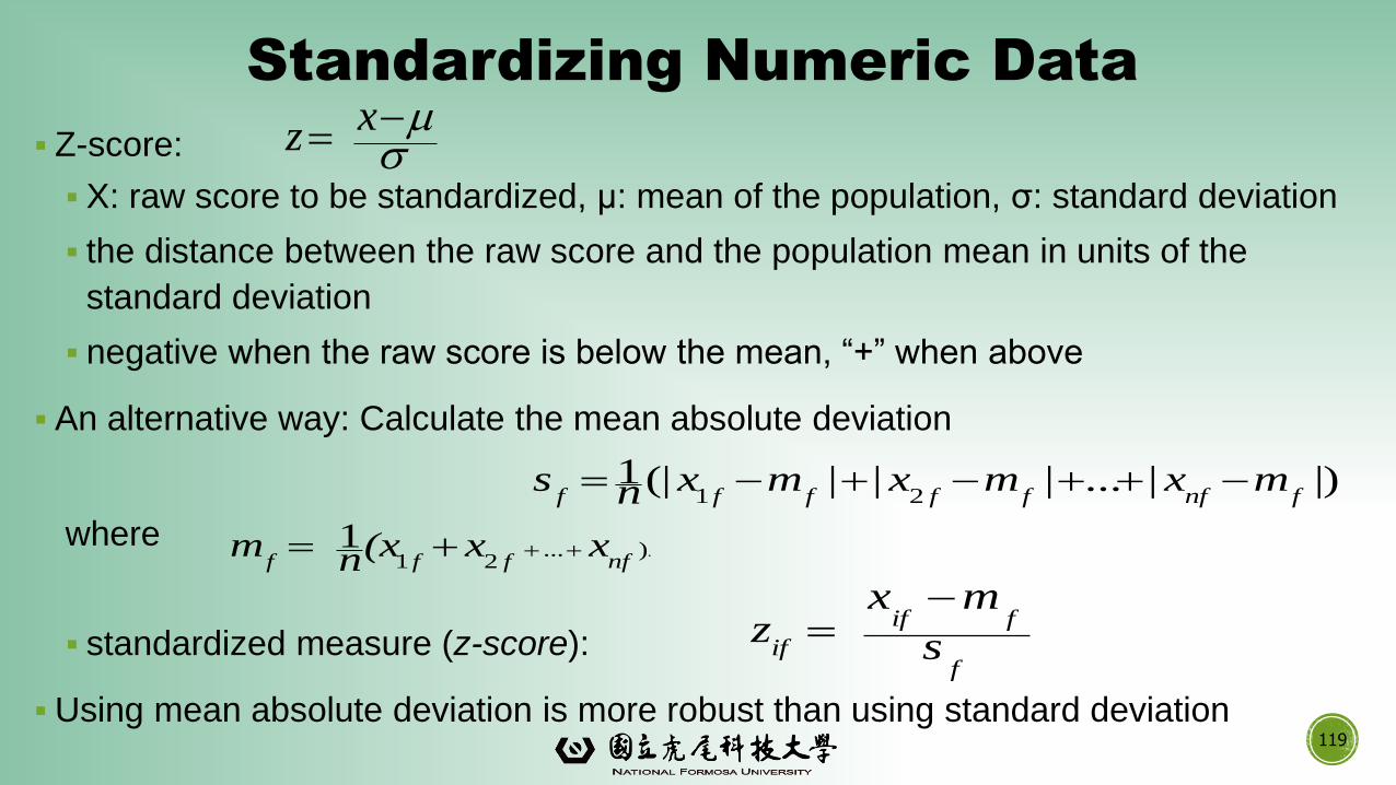
Standardizing Numeric Data
▪ Z-score:
▪ X: raw score to be standardized, μ: mean of the population, σ: standard deviation
▪ the distance between the raw score and the population mean in units of the
standard deviation
▪ negative when the raw score is below the mean, “+” when above
▪ An alternative way: Calculate the mean absolute deviation
where
▪ standardized measure (z-score):
▪Using mean absolute deviation is more robust than using standard deviation
x
z
119
.)...21
1nffff
xx(xn m
|)|...|||(|121 fnffffff
mxmxmxns
f
fif
if s
mx z
120
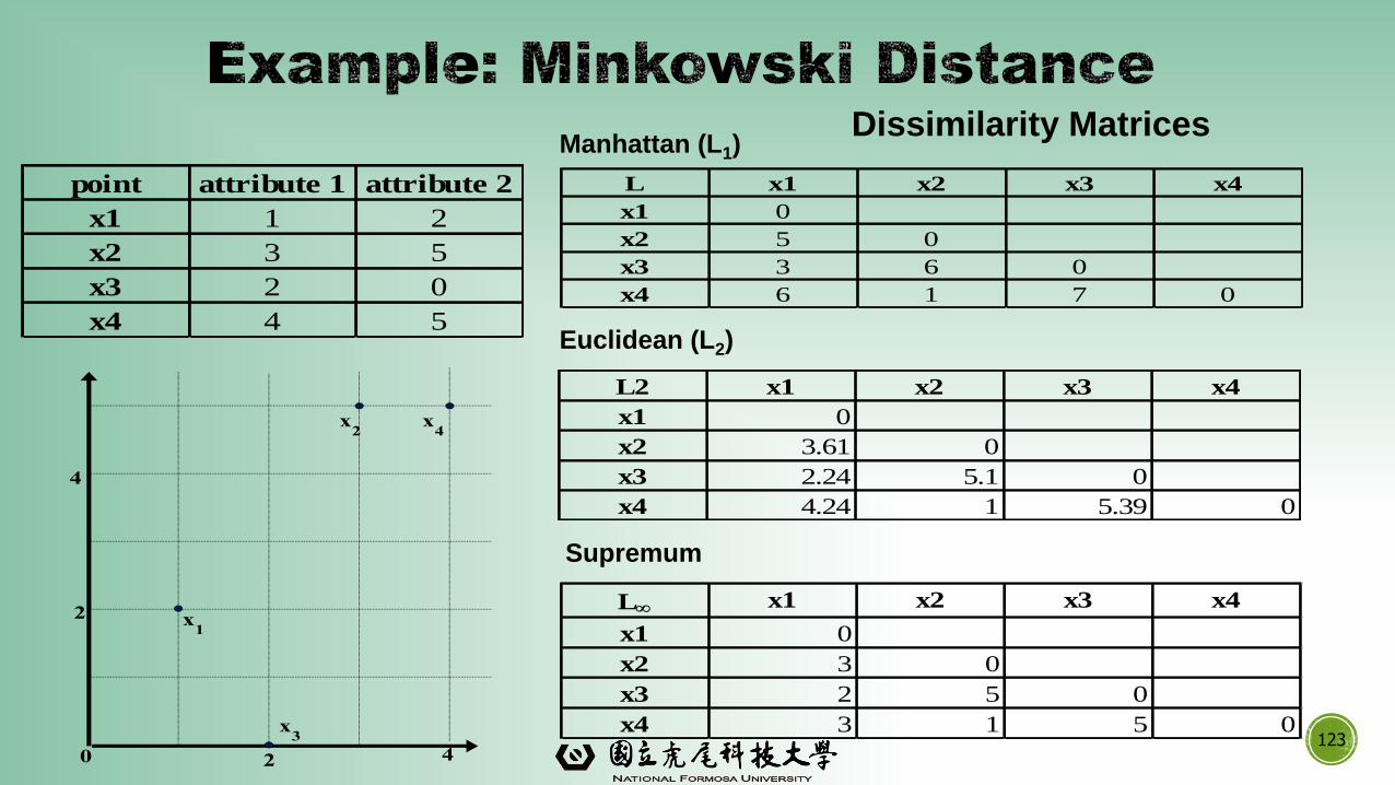
point attribute1 attribute2
x1 1 2
x2 3 5
x3 2 0
x4 4 5
Dissimilarity Matrix
(with Euclidean Distance)
x1 x2 x3 x4
x1 0
x2 3.61 0
x3 5.1 5.1 0
x4 4.24 1 5.39 0
Data Matrix
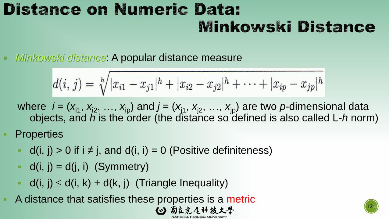
▪ Minkowski distance: A popular distance measure
where i = (xi1, xi2, …, xip) and j = (xj1, xj2, …, xjp) are two p-dimensional data objects, and h is the order (the distance so defined is also called L-h norm)
▪ Properties
▪ d(i, j) > 0 if i ≠ j, and d(i, i) = 0 (Positive definiteness)
▪ d(i, j) = d(j, i) (Symmetry)
▪ d(i, j) d(i, k) + d(k, j) (Triangle Inequality)
▪ A distance that satisfies these properties is a metric121
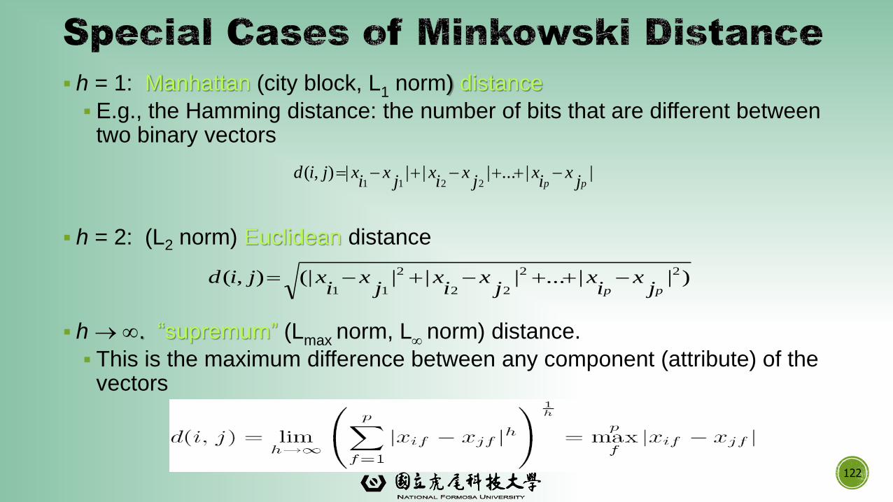
▪ h = 1: Manhattan (city block, L1 norm) distance
▪ E.g., the Hamming distance: the number of bits that are different between two binary vectors
▪ h = 2: (L2 norm) Euclidean distance
▪ h . “supremum” (Lmax norm, L norm) distance.
▪ This is the maximum difference between any component (attribute) of the vectors
||...||||),(2211 pp j
xi
xj
xi
xj
xi
xjid
122
)||...|||(|),( 22
22
2
11 pp jx
ix
jx
ix
jx
ixjid
123
Dissimilarity Matrices
point attribute 1 attribute 2
x1 1 2
x2 3 5
x3 2 0
x4 4 5
L x1 x2 x3 x4
x1 0
x2 5 0
x3 3 6 0
x4 6 1 7 0
L2 x1 x2 x3 x4
x1 0
x2 3.61 0
x3 2.24 5.1 0
x4 4.24 1 5.39 0
L x1 x2 x3 x4
x1 0
x2 3 0
x3 2 5 0
x4 3 1 5 0
Manhattan (L1)
Euclidean (L2)
Supremum
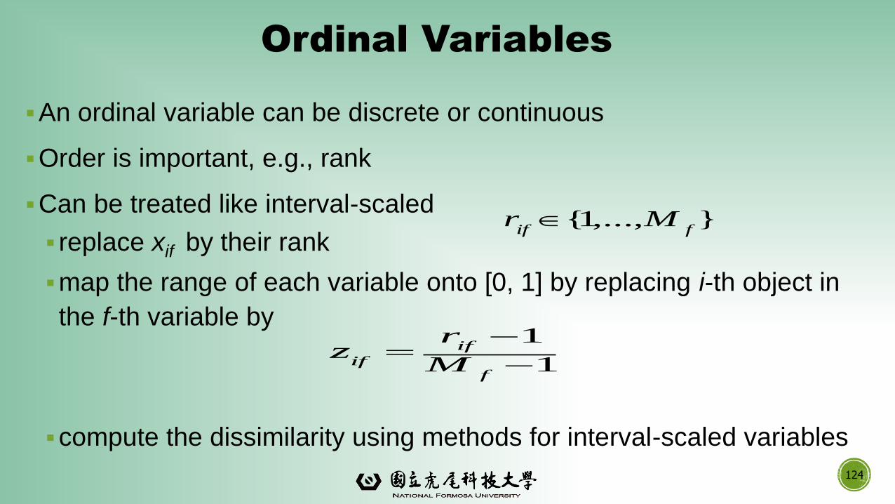
Ordinal Variables
▪An ordinal variable can be discrete or continuous
▪Order is important, e.g., rank
▪Can be treated like interval-scaled
▪ replace xif by their rank
▪map the range of each variable onto [0, 1] by replacing i-th object in
the f-th variable by
▪compute the dissimilarity using methods for interval-scaled variables
124
1
1
f
if
if M
rz
},...,1{fif
Mr

Attributes of Mixed Type
▪A database may contain all attribute types
▪Nominal, symmetric binary, asymmetric binary, numeric, ordinal
▪One may use a weighted formula to combine their effects
▪ f is binary or nominal:dij
(f) = 0 if xif = xjf , or dij(f) = 1 otherwise
▪ f is numeric: use the normalized distance
▪ f is ordinal ▪ Compute ranks rif and
▪ Treat zif as interval-scaled
)(1
)()(1),(
fij
pf
fij
fij
pf
djid
1
1
f
if
Mr
zif
125
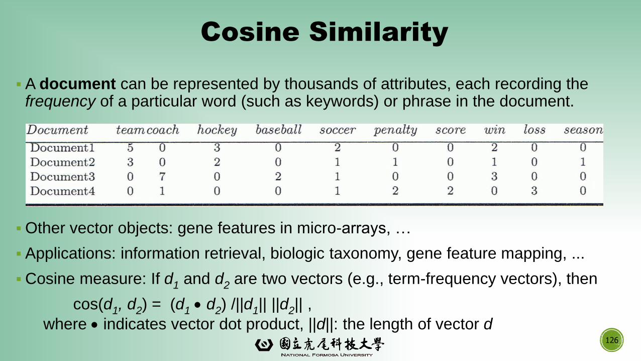
Cosine Similarity
▪ A document can be represented by thousands of attributes, each recording the frequency of a particular word (such as keywords) or phrase in the document.
▪Other vector objects: gene features in micro-arrays, …
▪ Applications: information retrieval, biologic taxonomy, gene feature mapping, ...
▪Cosine measure: If d1 and d2 are two vectors (e.g., term-frequency vectors), then
cos(d1, d2) = (d1 • d2) /||d1|| ||d2|| ,
where • indicates vector dot product, ||d||: the length of vector d126
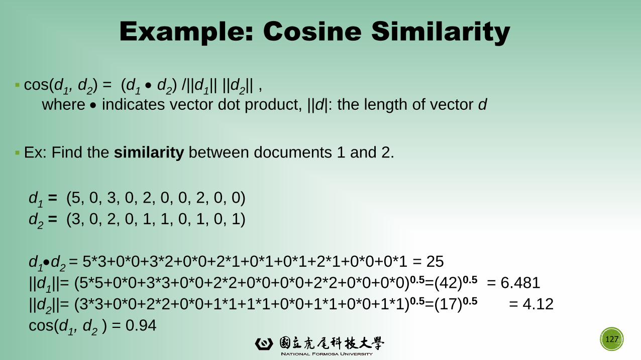
Example: Cosine Similarity
▪ cos(d1, d2) = (d1 • d2) /||d1|| ||d2|| ,
where • indicates vector dot product, ||d|: the length of vector d
▪ Ex: Find the similarity between documents 1 and 2.
d1 = (5, 0, 3, 0, 2, 0, 0, 2, 0, 0)
d2 = (3, 0, 2, 0, 1, 1, 0, 1, 0, 1)
d1•d2 = 5*3+0*0+3*2+0*0+2*1+0*1+0*1+2*1+0*0+0*1 = 25
||d1||= (5*5+0*0+3*3+0*0+2*2+0*0+0*0+2*2+0*0+0*0)0.5=(42)0.5 = 6.481
||d2||= (3*3+0*0+2*2+0*0+1*1+1*1+0*0+1*1+0*0+1*1)0.5=(17)0.5 = 4.12
cos(d1, d2 ) = 0.94127
Data Objects and Attribute Types
Basic Statistical Descriptions of Data
Data Visualization
Measuring Data Similarity and Dissimilarity
Summary
128
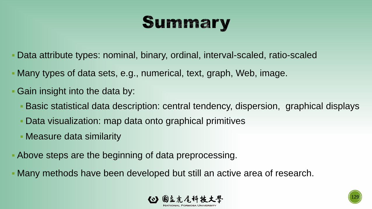
▪Data attribute types: nominal, binary, ordinal, interval-scaled, ratio-scaled
▪Many types of data sets, e.g., numerical, text, graph, Web, image.
▪Gain insight into the data by:
▪ Basic statistical data description: central tendency, dispersion, graphical displays
▪Data visualization: map data onto graphical primitives
▪Measure data similarity
▪ Above steps are the beginning of data preprocessing.
▪Many methods have been developed but still an active area of research.
129
W. Cleveland, Visualizing Data, Hobart Press, 1993
T. Dasu and T. Johnson. Exploratory Data Mining and Data Cleaning. John Wiley, 2003
U. Fayyad, G. Grinstein, and A. Wierse. Information Visualization in Data Mining and Knowledge Discovery, Morgan Kaufmann, 2001
L. Kaufman and P. J. Rousseeuw. Finding Groups in Data: an Introduction to Cluster Analysis. John Wiley & Sons, 1990.
H. V. Jagadish, et al., Special Issue on Data Reduction Techniques. Bulletin of the Tech. Committee on Data Eng., 20(4), Dec. 1997
D. A. Keim. Information visualization and visual data mining, IEEE trans. on Visualization and Computer Graphics, 8(1), 2002
D. Pyle. Data Preparation for Data Mining. Morgan Kaufmann, 1999
S. Santini and R. Jain,” Similarity measures”, IEEE Trans. on Pattern Analysis and Machine Intelligence, 21(9), 1999
E. R. Tufte. The Visual Display of Quantitative Information, 2nd ed., Graphics Press, 2001
C. Yu , et al., Visual data mining of multimedia data for social and behavioral studies, Information Visualization, 8(1), 2009
130
Data Preprocessing: An Overview
➢Data Quality
➢Major Tasks in Data Preprocessing
Data Cleaning
Data Integration
131
131

Data Reduction
Data Transformation and Data Discretization
Summary
132
132
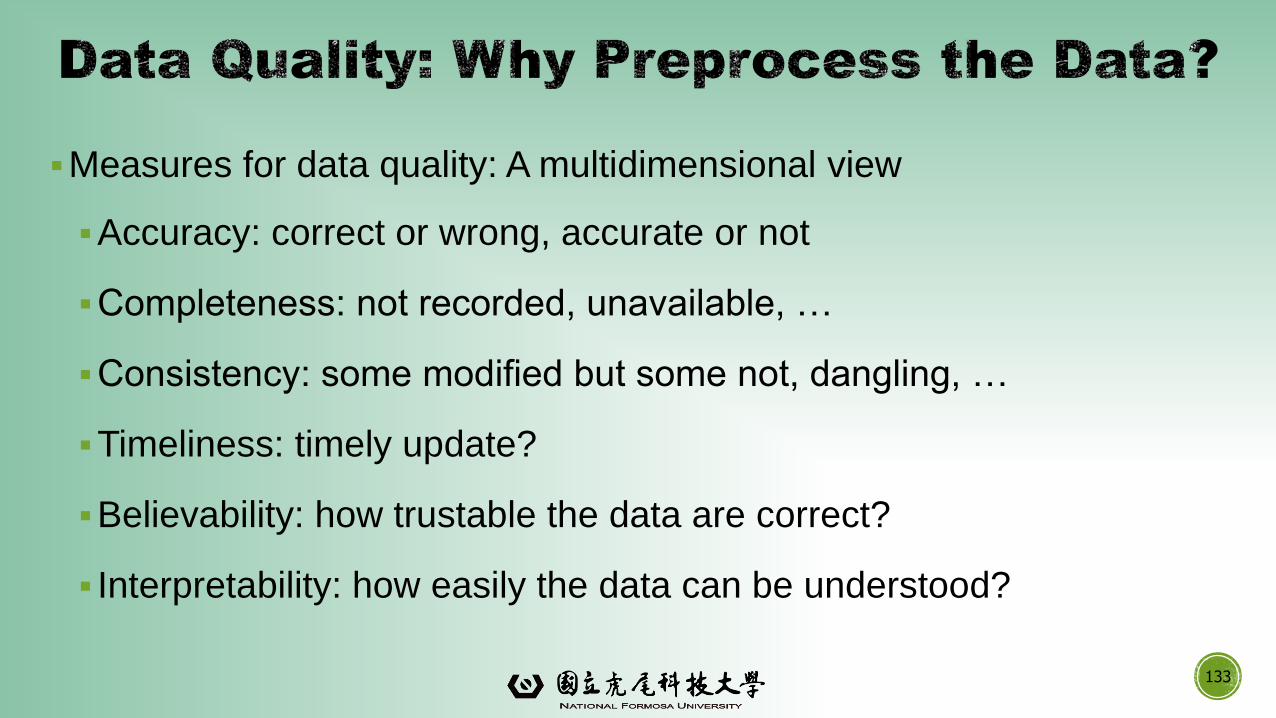
▪Measures for data quality: A multidimensional view
▪Accuracy: correct or wrong, accurate or not
▪Completeness: not recorded, unavailable, …
▪Consistency: some modified but some not, dangling, …
▪Timeliness: timely update?
▪Believability: how trustable the data are correct?
▪ Interpretability: how easily the data can be understood?
133
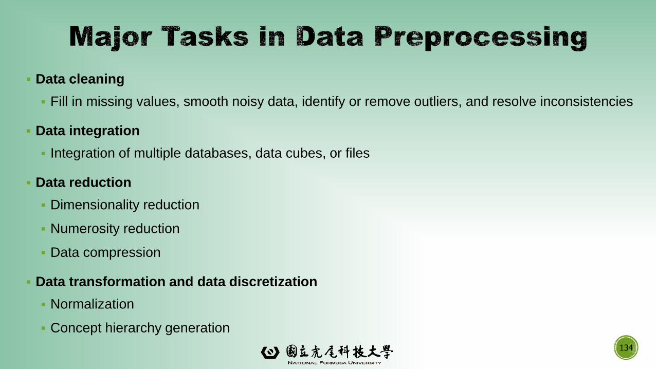
▪ Data cleaning
▪ Fill in missing values, smooth noisy data, identify or remove outliers, and resolve inconsistencies
▪ Data integration
▪ Integration of multiple databases, data cubes, or files
▪ Data reduction
▪ Dimensionality reduction
▪ Numerosity reduction
▪ Data compression
▪ Data transformation and data discretization
▪ Normalization
▪ Concept hierarchy generation
134
Data Preprocessing: An Overview
➢Data Quality
➢Major Tasks in Data Preprocessing
Data Cleaning
Data Integration
135
135
Data Reduction
Data Transformation and Data Discretization
Summary
136
136
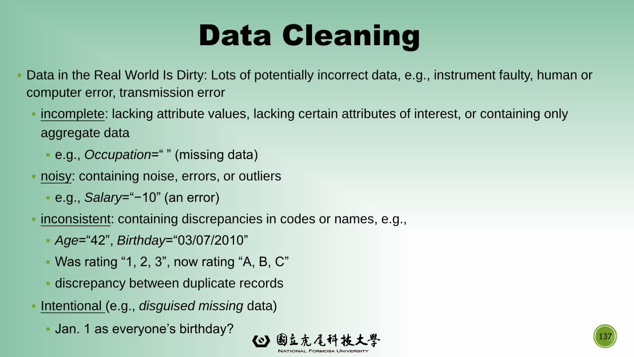
Data Cleaning
▪ Data in the Real World Is Dirty: Lots of potentially incorrect data, e.g., instrument faulty, human or
computer error, transmission error
▪ incomplete: lacking attribute values, lacking certain attributes of interest, or containing only
aggregate data
▪ e.g., Occupation=“ ” (missing data)
▪ noisy: containing noise, errors, or outliers
▪ e.g., Salary=“−10” (an error)
▪ inconsistent: containing discrepancies in codes or names, e.g.,
▪ Age=“42”, Birthday=“03/07/2010”
▪ Was rating “1, 2, 3”, now rating “A, B, C”
▪ discrepancy between duplicate records
▪ Intentional (e.g., disguised missing data)
▪ Jan. 1 as everyone’s birthday?137
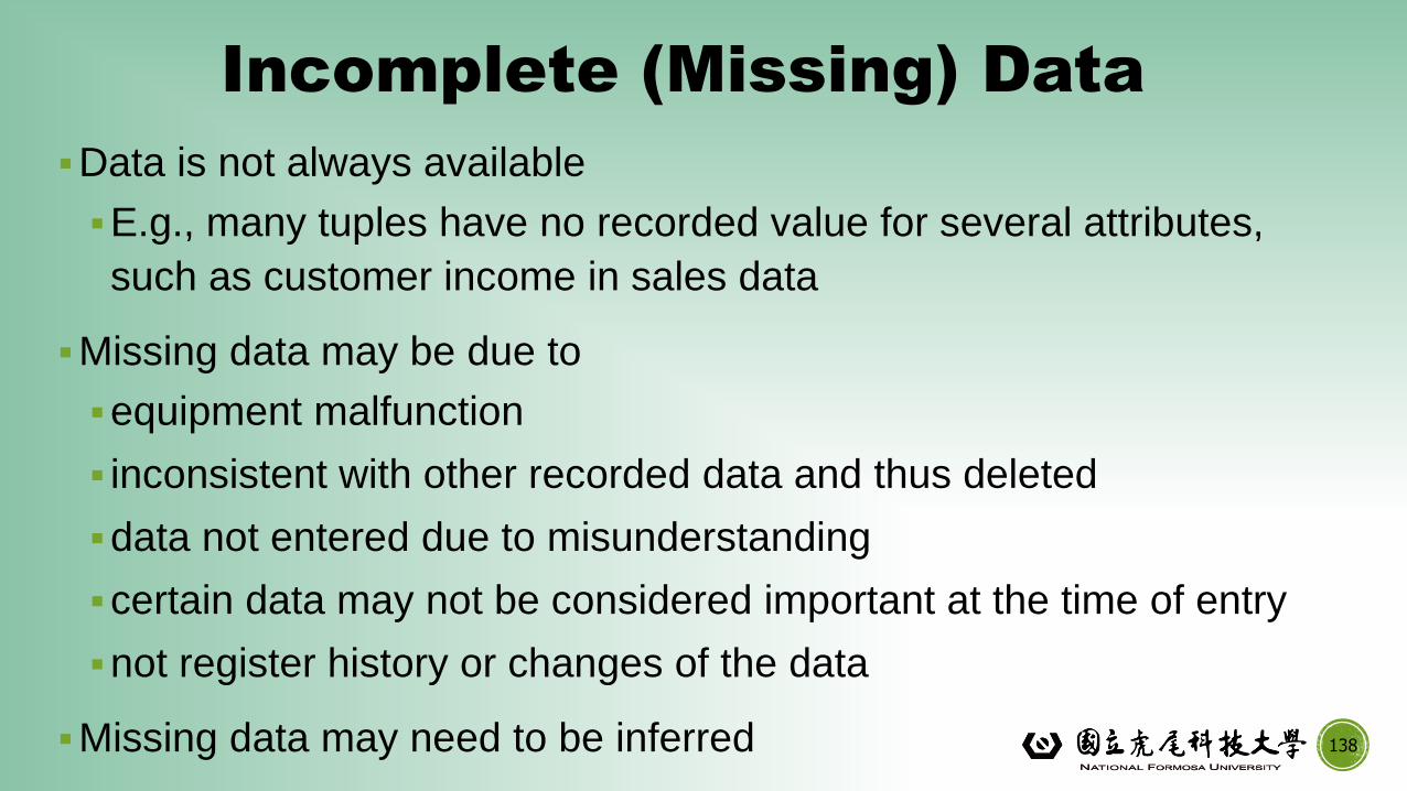
Incomplete (Missing) Data
▪Data is not always available
▪E.g., many tuples have no recorded value for several attributes,
such as customer income in sales data
▪Missing data may be due to
▪equipment malfunction
▪ inconsistent with other recorded data and thus deleted
▪data not entered due to misunderstanding
▪certain data may not be considered important at the time of entry
▪not register history or changes of the data
▪Missing data may need to be inferred 138
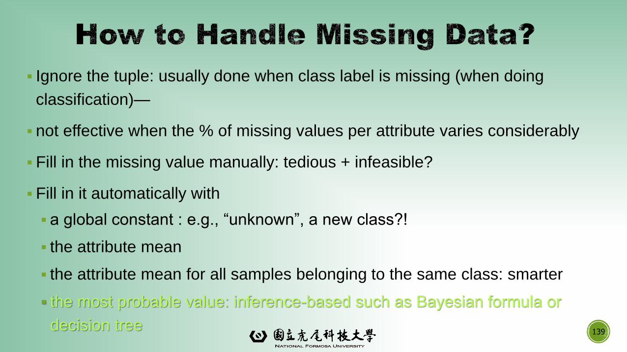
▪ Ignore the tuple: usually done when class label is missing (when doing
classification)—
▪ not effective when the % of missing values per attribute varies considerably
▪ Fill in the missing value manually: tedious + infeasible?
▪ Fill in it automatically with
▪ a global constant : e.g., “unknown”, a new class?!
▪ the attribute mean
▪ the attribute mean for all samples belonging to the same class: smarter
▪ the most probable value: inference-based such as Bayesian formula or
decision tree139
140
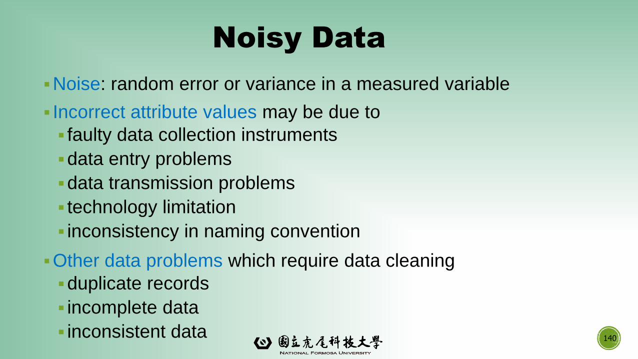
Noisy Data
▪Noise: random error or variance in a measured variable
▪ Incorrect attribute values may be due to
▪ faulty data collection instruments
▪data entry problems
▪data transmission problems
▪ technology limitation
▪ inconsistency in naming convention
▪Other data problems which require data cleaning
▪duplicate records
▪ incomplete data
▪ inconsistent data
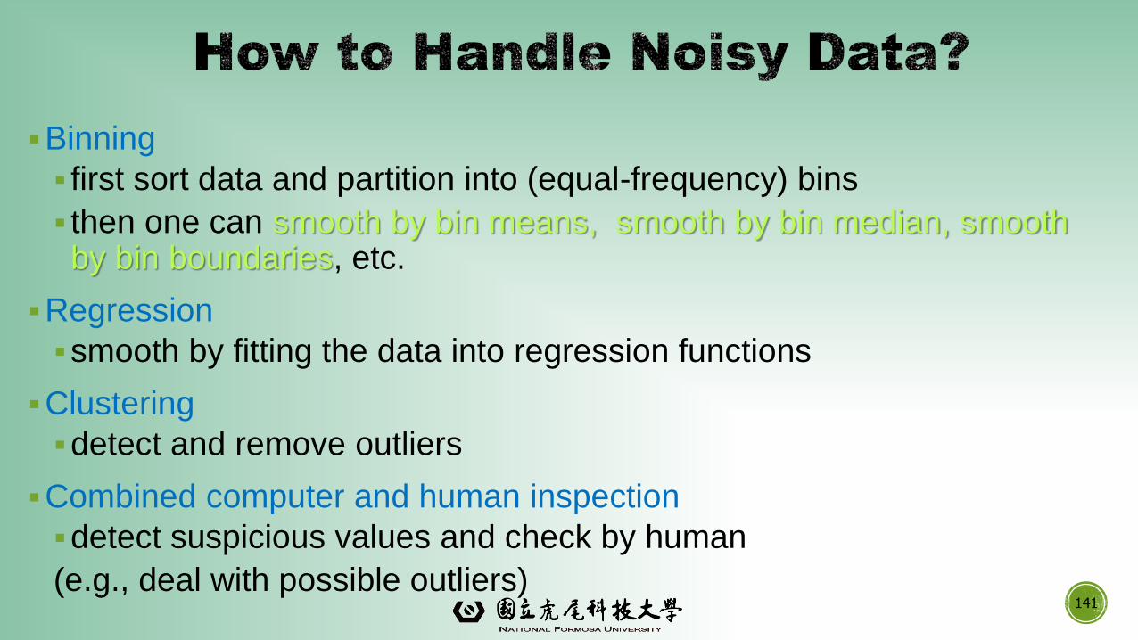
▪Binning
▪ first sort data and partition into (equal-frequency) bins
▪ then one can smooth by bin means, smooth by bin median, smooth by bin boundaries, etc.
▪Regression
▪smooth by fitting the data into regression functions
▪Clustering
▪detect and remove outliers
▪Combined computer and human inspection
▪detect suspicious values and check by human
(e.g., deal with possible outliers)141
Data Cleaning as a Process
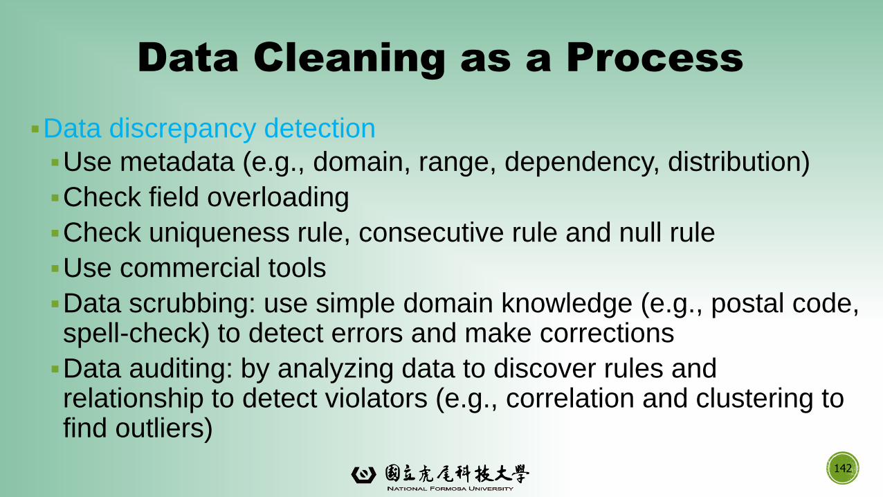
▪Data discrepancy detection
▪Use metadata (e.g., domain, range, dependency, distribution)
▪Check field overloading
▪Check uniqueness rule, consecutive rule and null rule
▪Use commercial tools
▪Data scrubbing: use simple domain knowledge (e.g., postal code, spell-check) to detect errors and make corrections
▪Data auditing: by analyzing data to discover rules and relationship to detect violators (e.g., correlation and clustering to find outliers)
142
Data Cleaning as a Process
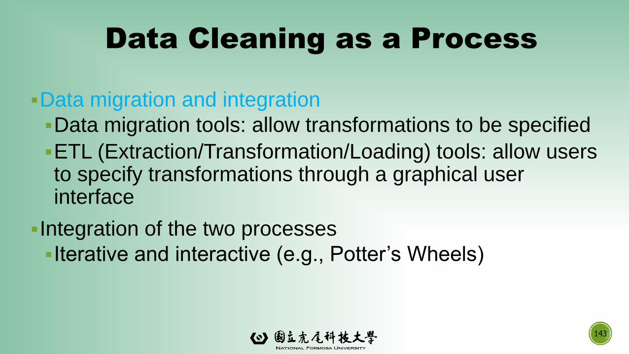
▪Data migration and integration
▪Data migration tools: allow transformations to be specified
▪ETL (Extraction/Transformation/Loading) tools: allow users to specify transformations through a graphical user interface
▪Integration of the two processes
▪Iterative and interactive (e.g., Potter’s Wheels)
143
Data Preprocessing: An Overview
➢Data Quality
➢Major Tasks in Data Preprocessing
Data Cleaning
Data Integration
144
Data Reduction
Data Transformation and Data Discretization
Summary
145
Data Integration
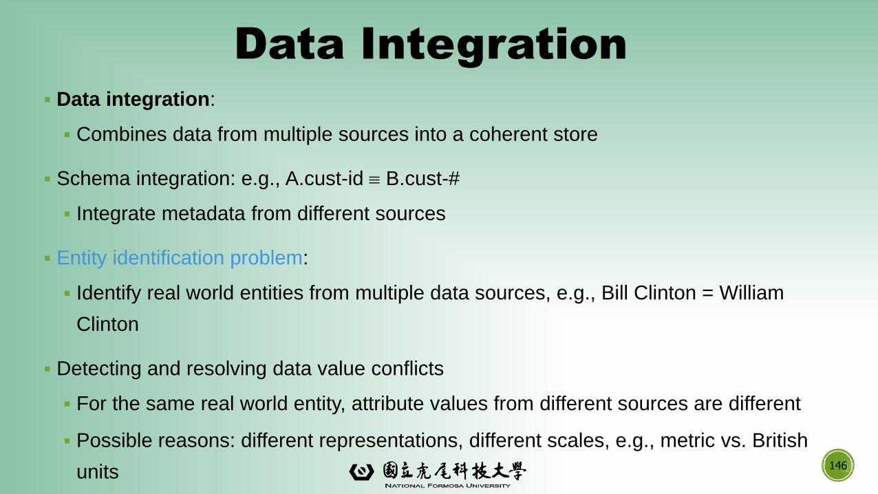
▪ Data integration:
▪ Combines data from multiple sources into a coherent store
▪ Schema integration: e.g., A.cust-id B.cust-#
▪ Integrate metadata from different sources
▪ Entity identification problem:
▪ Identify real world entities from multiple data sources, e.g., Bill Clinton = William
Clinton
▪ Detecting and resolving data value conflicts
▪ For the same real world entity, attribute values from different sources are different
▪ Possible reasons: different representations, different scales, e.g., metric vs. British
units 146
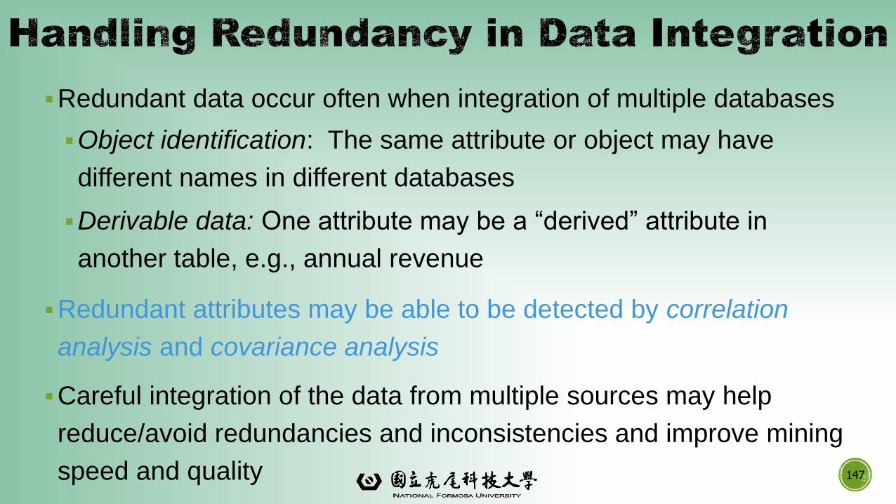
▪Redundant data occur often when integration of multiple databases
▪Object identification: The same attribute or object may have
different names in different databases
▪Derivable data: One attribute may be a “derived” attribute in
another table, e.g., annual revenue
▪Redundant attributes may be able to be detected by correlation
analysis and covariance analysis
▪Careful integration of the data from multiple sources may help
reduce/avoid redundancies and inconsistencies and improve mining
speed and quality 147

▪Χ2 (chi-square) test
▪The larger the Χ2 value, the more likely the variables are related
▪The cells that contribute the most to the Χ2 value are those whose
actual count is very different from the expected count
▪Correlation does not imply causality
▪ # of hospitals and # of car-theft in a city are correlated
▪ Both are causally linked to the third variable: population
Expected
ExpectedObserved 22 )(
148
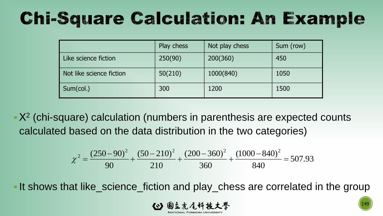
▪Χ2 (chi-square) calculation (numbers in parenthesis are expected counts
calculated based on the data distribution in the two categories)
▪ It shows that like_science_fiction and play_chess are correlated in the group
93.507840
)8401000(
360
)360200(
210
)21050(
90
)90250( 22222
149
Play chess Not play chess Sum (row)
Like science fiction 250(90) 200(360) 450
Not like science fiction 50(210) 1000(840) 1050
Sum(col.) 300 1200 1500
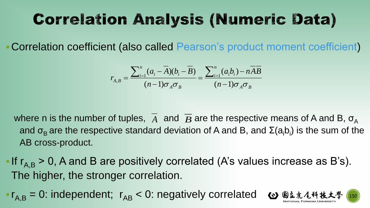
▪Correlation coefficient (also called Pearson’s product moment coefficient)
where n is the number of tuples, and are the respective means of A and B, σA
and σB are the respective standard deviation of A and B, and Σ(aibi) is the sum of the
AB cross-product.
▪ If rA,B > 0, A and B are positively correlated (A’s values increase as B’s).
The higher, the stronger correlation.
▪ rA,B = 0: independent; rAB < 0: negatively correlated
BA
n
i ii
BA
n
i ii
BAn
BAnba
n
BbAar
)1(
)(
)1(
))((11
,
A
150
B
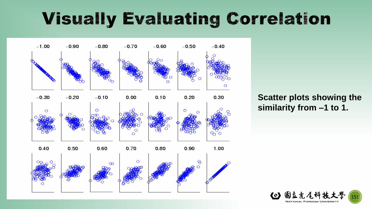
151
Scatter plots showing the
similarity from –1 to 1.
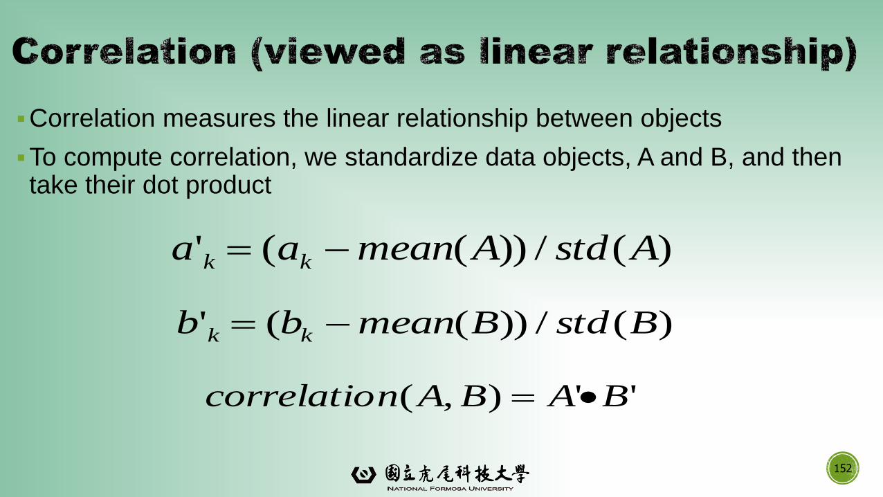
▪Correlation measures the linear relationship between objects
▪To compute correlation, we standardize data objects, A and B, and then take their dot product
152
)(/))((' AstdAmeanaa kk
)(/))((' BstdBmeanbb kk
''),( BABAncorrelatio •
▪ Covariance is similar to correlation
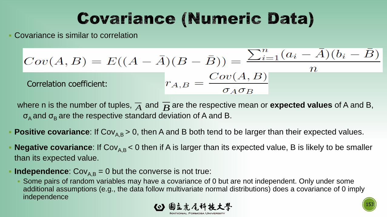
where n is the number of tuples, and are the respective mean or expected values of A and B,
σA and σB are the respective standard deviation of A and B.
▪ Positive covariance: If CovA,B > 0, then A and B both tend to be larger than their expected values.
▪ Negative covariance: If CovA,B < 0 then if A is larger than its expected value, B is likely to be smaller
than its expected value.
▪ Independence: CovA,B = 0 but the converse is not true:
▪ Some pairs of random variables may have a covariance of 0 but are not independent. Only under some additional assumptions (e.g., the data follow multivariate normal distributions) does a covariance of 0 imply independence
153
A B
Correlation coefficient:
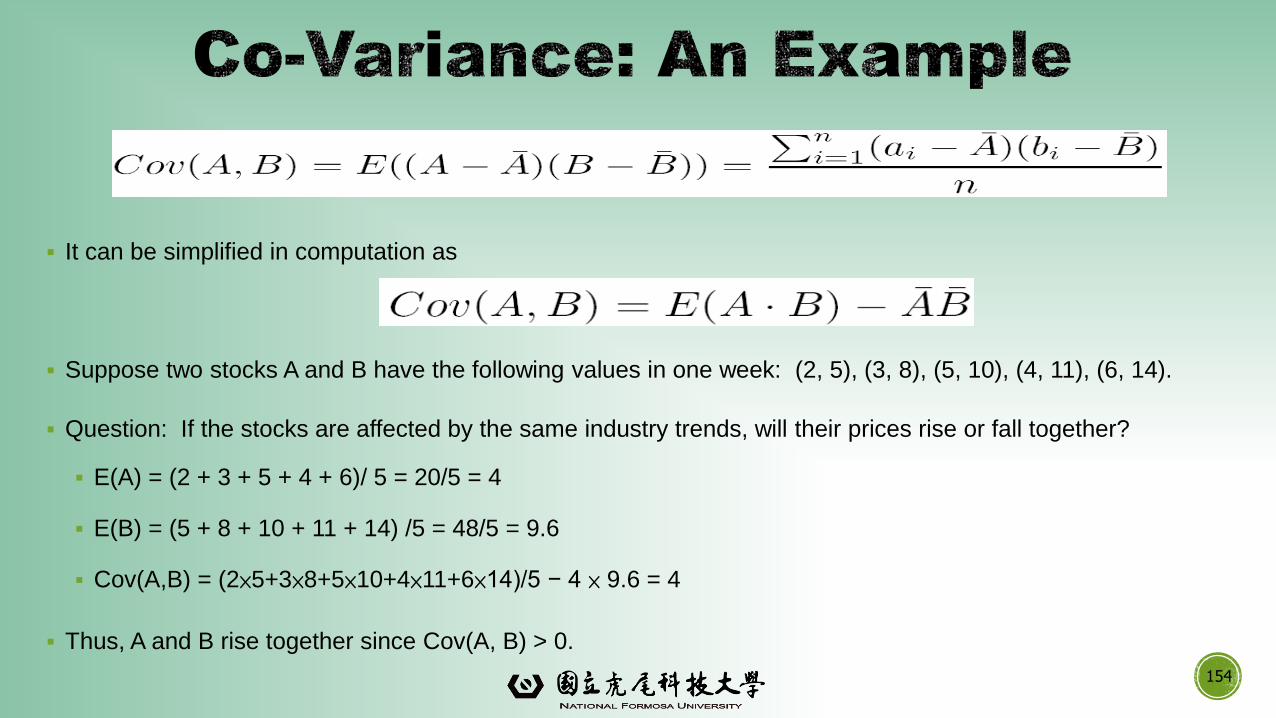
▪ It can be simplified in computation as
▪ Suppose two stocks A and B have the following values in one week: (2, 5), (3, 8), (5, 10), (4, 11), (6, 14).
▪ Question: If the stocks are affected by the same industry trends, will their prices rise or fall together?
▪ E(A) = (2 + 3 + 5 + 4 + 6)/ 5 = 20/5 = 4
▪ E(B) = (5 + 8 + 10 + 11 + 14) /5 = 48/5 = 9.6
▪ Cov(A,B) = (2×5+3×8+5×10+4×11+6×14)/5 − 4 × 9.6 = 4
▪ Thus, A and B rise together since Cov(A, B) > 0.
154
Data Preprocessing: An Overview
➢Data Quality
➢Major Tasks in Data Preprocessing
Data Cleaning
Data Integration
155
Data Reduction
Data Transformation and Data Discretization
Summary
156
▪Data reduction:
Obtain a reduced representation of the data set that is much smaller in volume but yet produces the same (or almost the same) analytical results.
▪Why data reduction?
— A database/data warehouse may store terabytes of data. Complex data analysis may take a very long time to run on the complete data set.
157
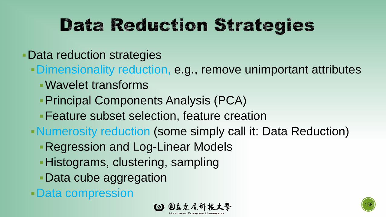
▪Data reduction strategies
▪Dimensionality reduction, e.g., remove unimportant attributes
▪Wavelet transforms
▪Principal Components Analysis (PCA)
▪Feature subset selection, feature creation
▪Numerosity reduction (some simply call it: Data Reduction)
▪Regression and Log-Linear Models
▪Histograms, clustering, sampling
▪Data cube aggregation
▪Data compression158
159
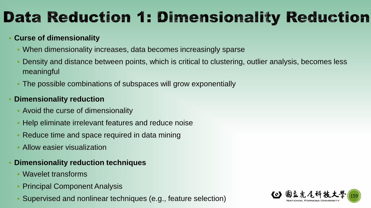
▪ Curse of dimensionality
▪ When dimensionality increases, data becomes increasingly sparse
▪ Density and distance between points, which is critical to clustering, outlier analysis, becomes less
meaningful
▪ The possible combinations of subspaces will grow exponentially
▪ Dimensionality reduction
▪ Avoid the curse of dimensionality
▪ Help eliminate irrelevant features and reduce noise
▪ Reduce time and space required in data mining
▪ Allow easier visualization
▪ Dimensionality reduction techniques
▪ Wavelet transforms
▪ Principal Component Analysis
▪ Supervised and nonlinear techniques (e.g., feature selection)
160
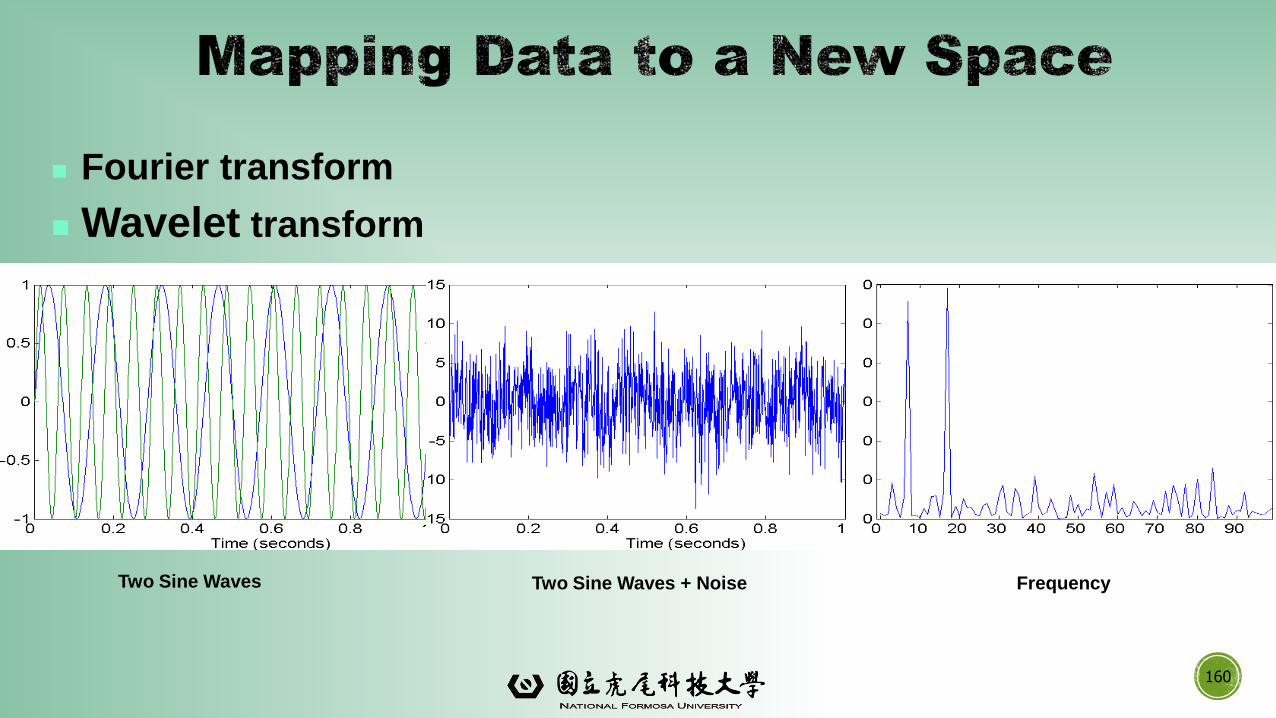
Two Sine Waves Two Sine Waves + Noise Frequency
Fourier transform
Wavelet transform
161
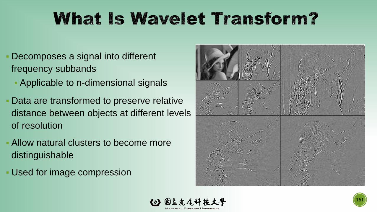
▪Decomposes a signal into different
frequency subbands
▪ Applicable to n-dimensional signals
▪Data are transformed to preserve relative
distance between objects at different levels
of resolution
▪ Allow natural clusters to become more
distinguishable
▪Used for image compression
162
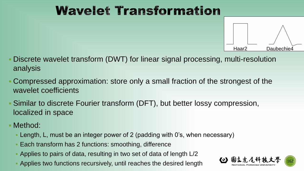
▪Discrete wavelet transform (DWT) for linear signal processing, multi-resolution
analysis
▪Compressed approximation: store only a small fraction of the strongest of the
wavelet coefficients
▪ Similar to discrete Fourier transform (DFT), but better lossy compression,
localized in space
▪Method:
▪ Length, L, must be an integer power of 2 (padding with 0’s, when necessary)
▪ Each transform has 2 functions: smoothing, difference
▪ Applies to pairs of data, resulting in two set of data of length L/2
▪ Applies two functions recursively, until reaches the desired length
Haar2 Daubechie4
163
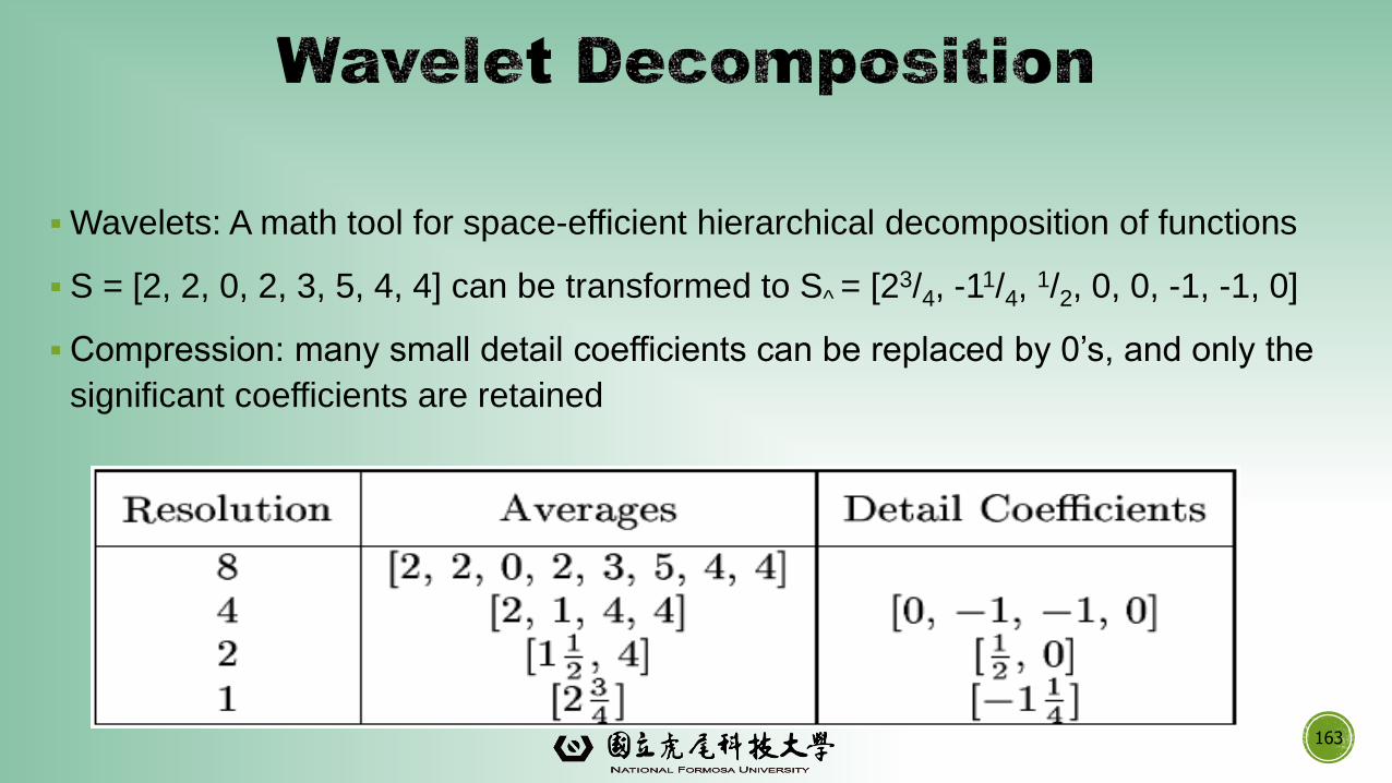
▪Wavelets: A math tool for space-efficient hierarchical decomposition of functions
▪ S = [2, 2, 0, 2, 3, 5, 4, 4] can be transformed to S^ = [23/4, -11/4,
1/2, 0, 0, -1, -1, 0]
▪Compression: many small detail coefficients can be replaced by 0’s, and only the
significant coefficients are retained
164
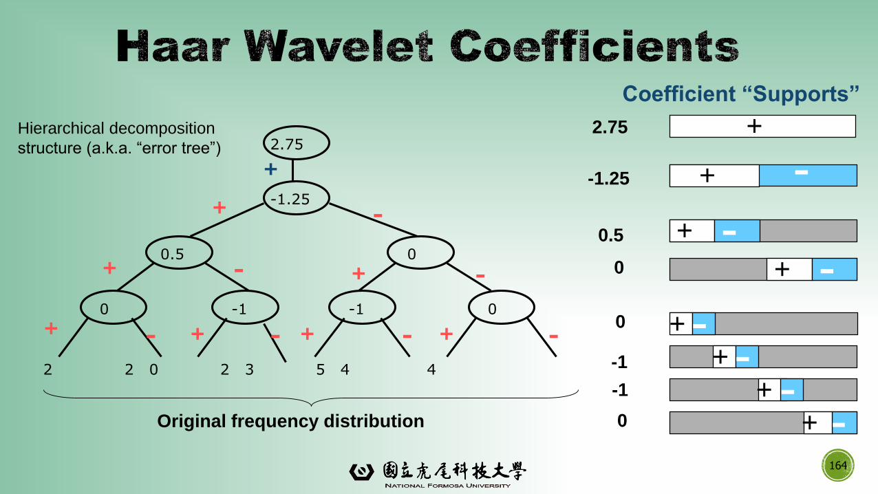
Coefficient “Supports”
2 2 0 2 3 5 4 4
-1.25
2.75
0.5 0
0 -1 0-1
+
-+
+
+ + +
+
+
- -
- - - -
+
-+
+ -+ -
+ -+ -
-+
+ --1
-1
0.5
0
2.75
-1.25
0
0Original frequency distribution
Hierarchical decomposition
structure (a.k.a. “error tree”)
165
▪Use hat-shape filters
▪Emphasize region where points cluster
▪Suppress weaker information in their boundaries
▪Effective removal of outliers
▪ Insensitive to noise, insensitive to input order
▪Multi-resolution
▪Detect arbitrary shaped clusters at different scales
▪Efficient
▪Complexity O(N)
▪Only applicable to low dimensional data
▪ Find a projection that captures the largest amount of variation in data
▪ The original data are projected onto a much smaller space, resulting in
dimensionality reduction. We find the eigenvectors of the covariance matrix, and
these eigenvectors define the new space
166
x2
x1
e
▪ Given N data vectors from n-dimensions, find k ≤ n orthogonal vectors (principal components)
that can be best used to represent data
▪ Normalize input data: Each attribute falls within the same range
▪ Compute k orthonormal (unit) vectors, i.e., principal components
▪ Each input data (vector) is a linear combination of the k principal component vectors
▪ The principal components are sorted in order of decreasing “significance” or strength
▪ Since the components are sorted, the size of the data can be reduced by eliminating the
weak components, i.e., those with low variance (i.e., using the strongest principal
components, it is possible to reconstruct a good approximation of the original data)
▪ Works for numeric data only
167
▪Another way to reduce dimensionality of data
▪Redundant attributes
▪Duplicate much or all of the information contained in one or more other
attributes
▪E.g., purchase price of a product and the amount of sales tax paid
▪ Irrelevant attributes
▪Contain no information that is useful for the data mining task at hand
▪E.g., students' ID is often irrelevant to the task of predicting students'
GPA168
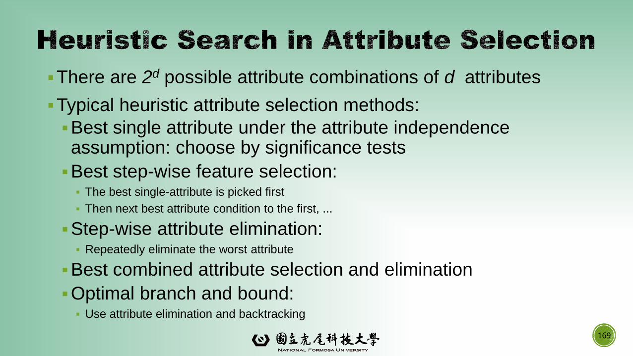
▪There are 2d possible attribute combinations of d attributes
▪Typical heuristic attribute selection methods:
▪Best single attribute under the attribute independence assumption: choose by significance tests
▪Best step-wise feature selection:▪ The best single-attribute is picked first
▪ Then next best attribute condition to the first, ...
▪Step-wise attribute elimination:▪ Repeatedly eliminate the worst attribute
▪Best combined attribute selection and elimination
▪Optimal branch and bound:▪ Use attribute elimination and backtracking
169
170
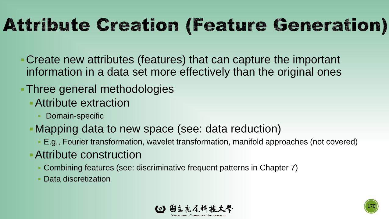
▪Create new attributes (features) that can capture the important information in a data set more effectively than the original ones
▪Three general methodologies
▪Attribute extraction▪ Domain-specific
▪Mapping data to new space (see: data reduction)▪ E.g., Fourier transformation, wavelet transformation, manifold approaches (not covered)
▪Attribute construction ▪ Combining features (see: discriminative frequent patterns in Chapter 7)
▪ Data discretization
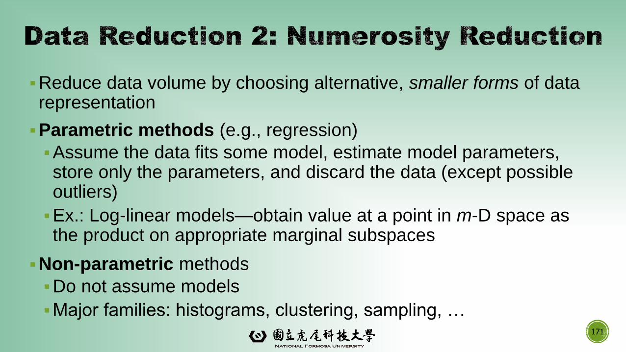
▪Reduce data volume by choosing alternative, smaller forms of data representation
▪Parametric methods (e.g., regression)
▪Assume the data fits some model, estimate model parameters, store only the parameters, and discard the data (except possible outliers)
▪Ex.: Log-linear models—obtain value at a point in m-D space as the product on appropriate marginal subspaces
▪Non-parametric methods
▪Do not assume models
▪Major families: histograms, clustering, sampling, … 171
Parametric Data Reduction:
Regression and Log-Linear Models
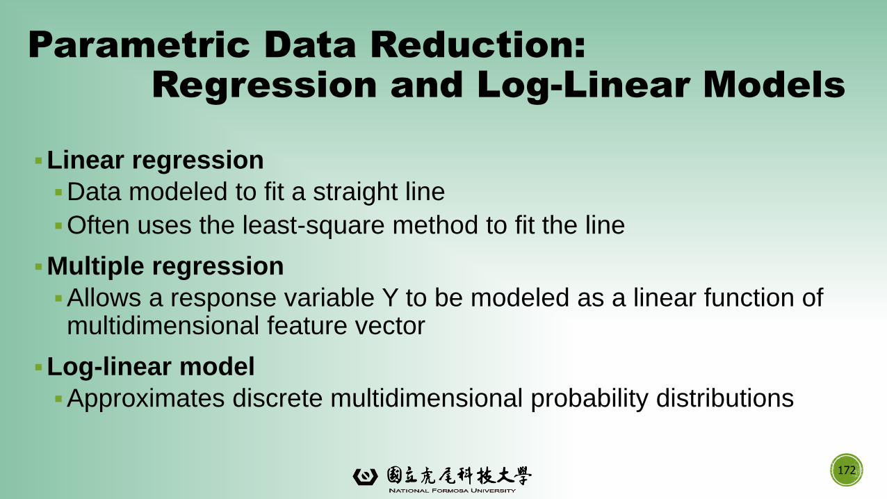
▪Linear regression
▪Data modeled to fit a straight line
▪Often uses the least-square method to fit the line
▪Multiple regression
▪Allows a response variable Y to be modeled as a linear function of multidimensional feature vector
▪Log-linear model
▪Approximates discrete multidimensional probability distributions
172
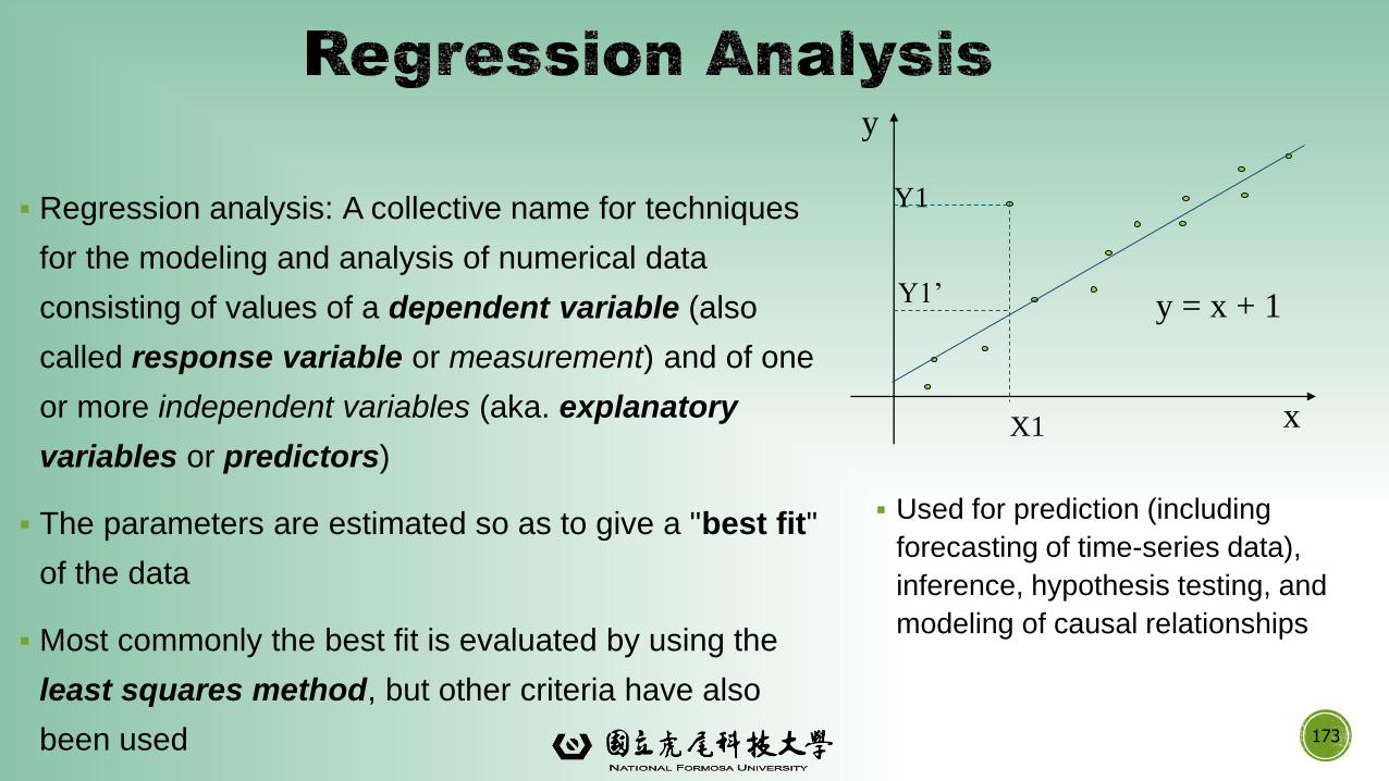
▪ Regression analysis: A collective name for techniques
for the modeling and analysis of numerical data
consisting of values of a dependent variable (also
called response variable or measurement) and of one
or more independent variables (aka. explanatory
variables or predictors)
▪ The parameters are estimated so as to give a "best fit"
of the data
▪ Most commonly the best fit is evaluated by using the
least squares method, but other criteria have also
been used
▪ Used for prediction (including
forecasting of time-series data),
inference, hypothesis testing, and
modeling of causal relationships
173
y
x
y = x + 1
X1
Y1
Y1’
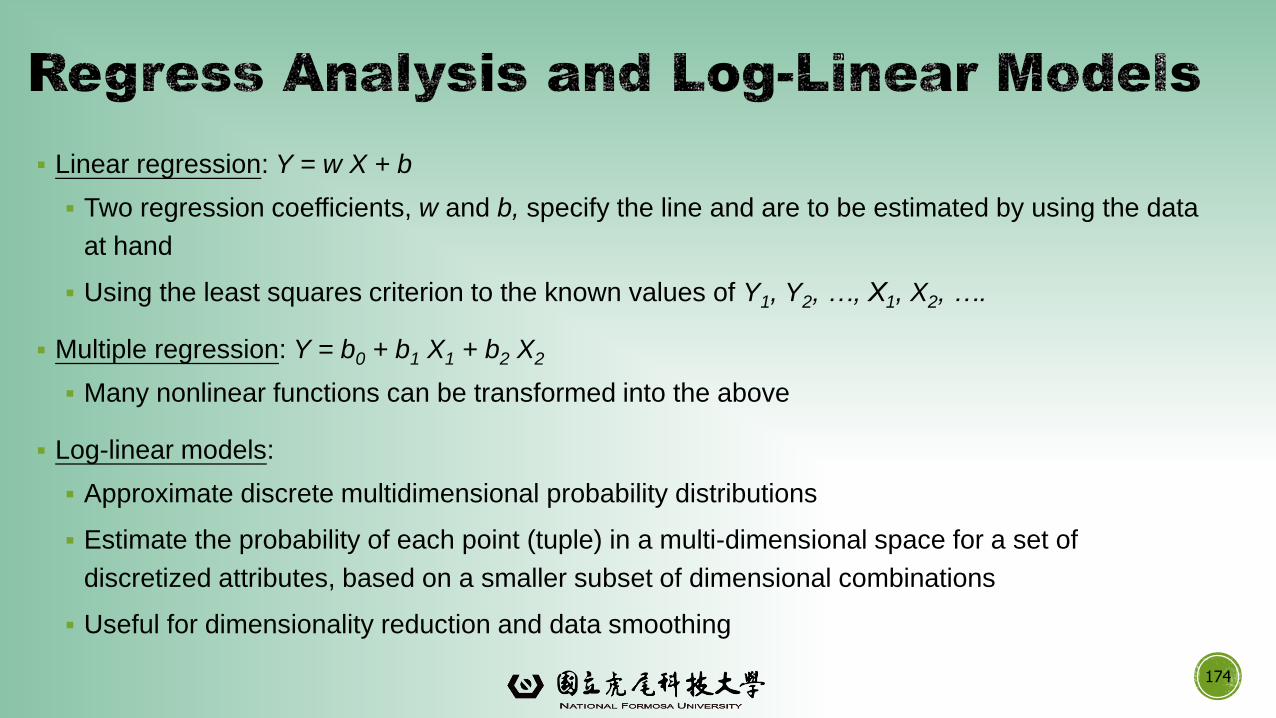
▪ Linear regression: Y = w X + b
▪ Two regression coefficients, w and b, specify the line and are to be estimated by using the data
at hand
▪ Using the least squares criterion to the known values of Y1, Y2, …, X1, X2, ….
▪ Multiple regression: Y = b0 + b1 X1 + b2 X2
▪ Many nonlinear functions can be transformed into the above
▪ Log-linear models:
▪ Approximate discrete multidimensional probability distributions
▪ Estimate the probability of each point (tuple) in a multi-dimensional space for a set of
discretized attributes, based on a smaller subset of dimensional combinations
▪ Useful for dimensionality reduction and data smoothing
174
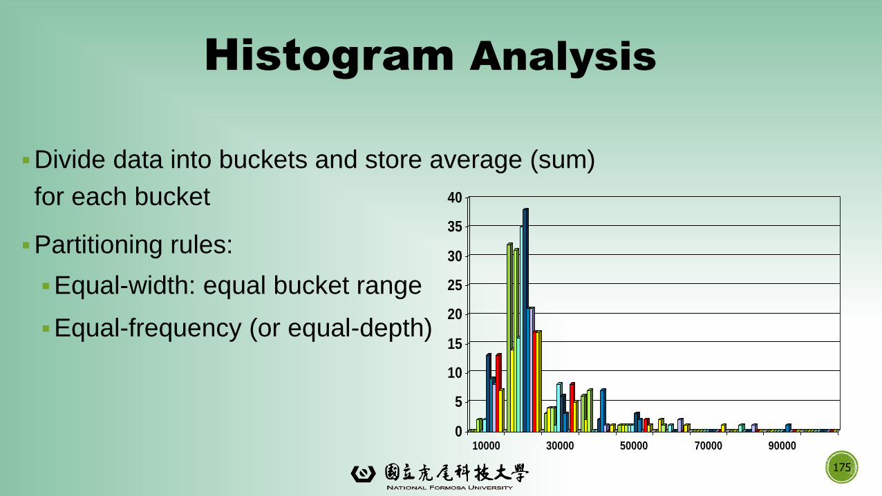
Histogram Analysis
▪Divide data into buckets and store average (sum)
for each bucket
▪Partitioning rules:
▪Equal-width: equal bucket range
▪Equal-frequency (or equal-depth)
175
0
5
10
15
20
25
30
35
40
10000 30000 50000 70000 90000
Clustering
▪Partition data set into clusters based on similarity, and store cluster
representation (e.g., centroid and diameter) only
▪Can be very effective if data is clustered but not if data is “smeared”
▪Can have hierarchical clustering and be stored in multi-dimensional
index tree structures
▪There are many choices of clustering definitions and clustering
algorithms
▪Cluster analysis will be studied in depth in Chapter 10
176
Sampling
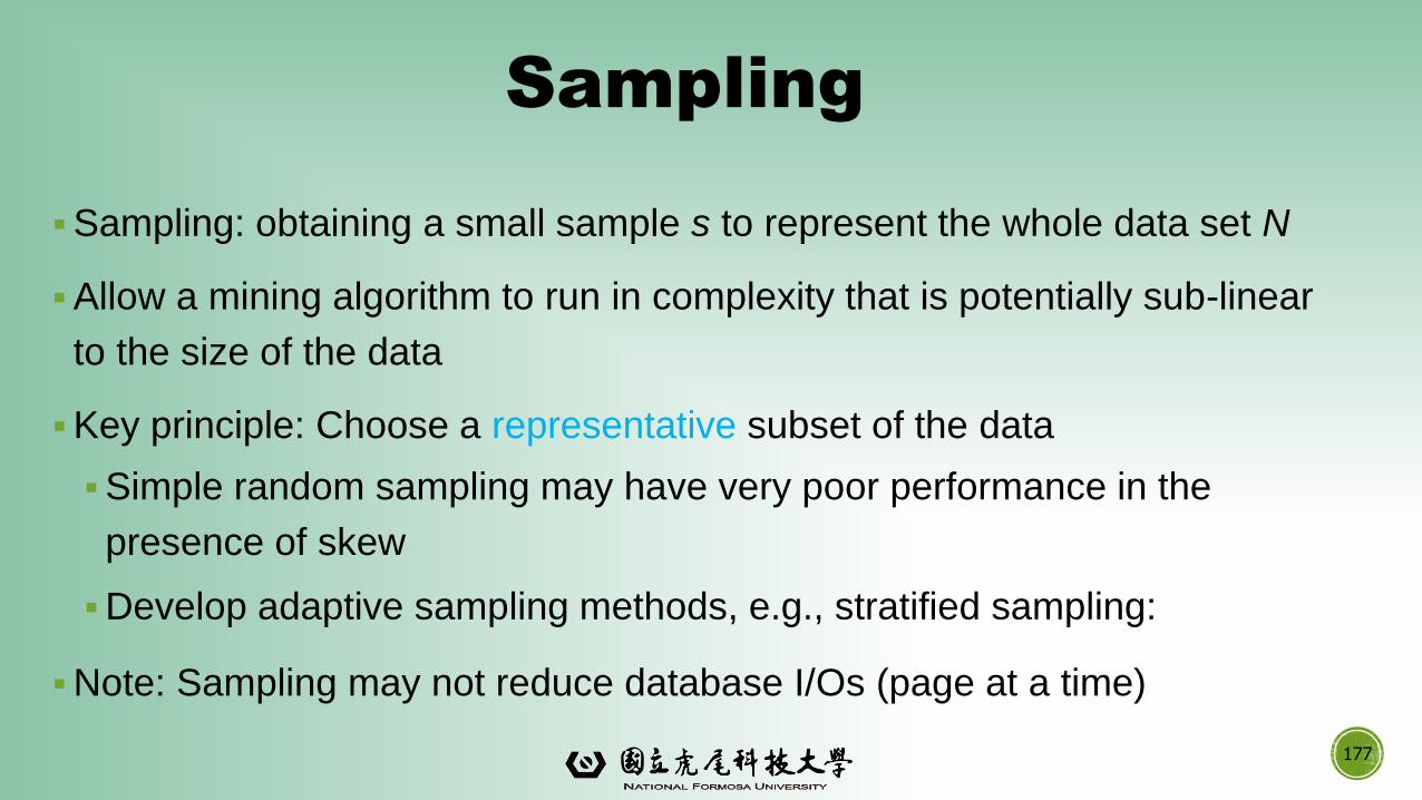
▪Sampling: obtaining a small sample s to represent the whole data set N
▪Allow a mining algorithm to run in complexity that is potentially sub-linear
to the size of the data
▪Key principle: Choose a representative subset of the data
▪Simple random sampling may have very poor performance in the
presence of skew
▪Develop adaptive sampling methods, e.g., stratified sampling:
▪Note: Sampling may not reduce database I/Os (page at a time)
177
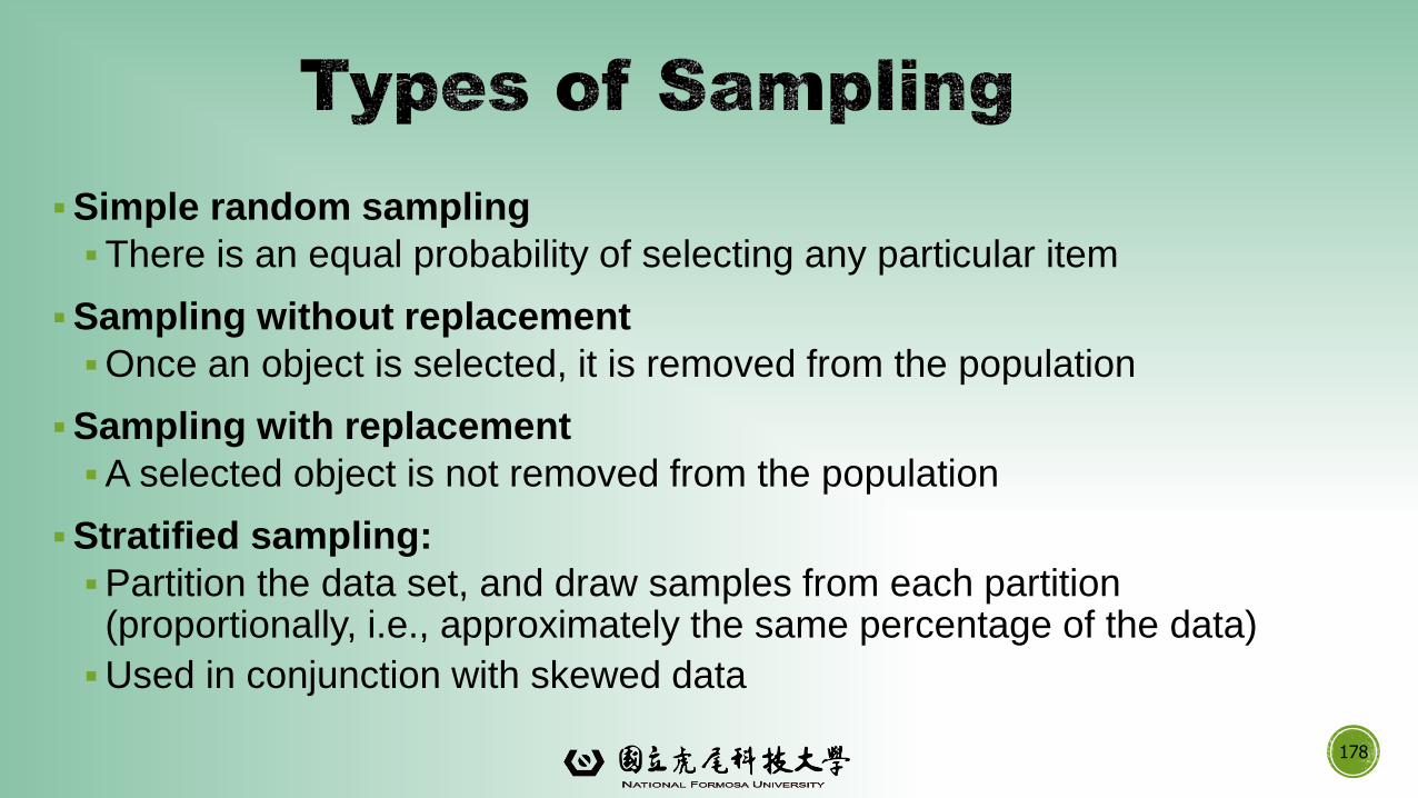
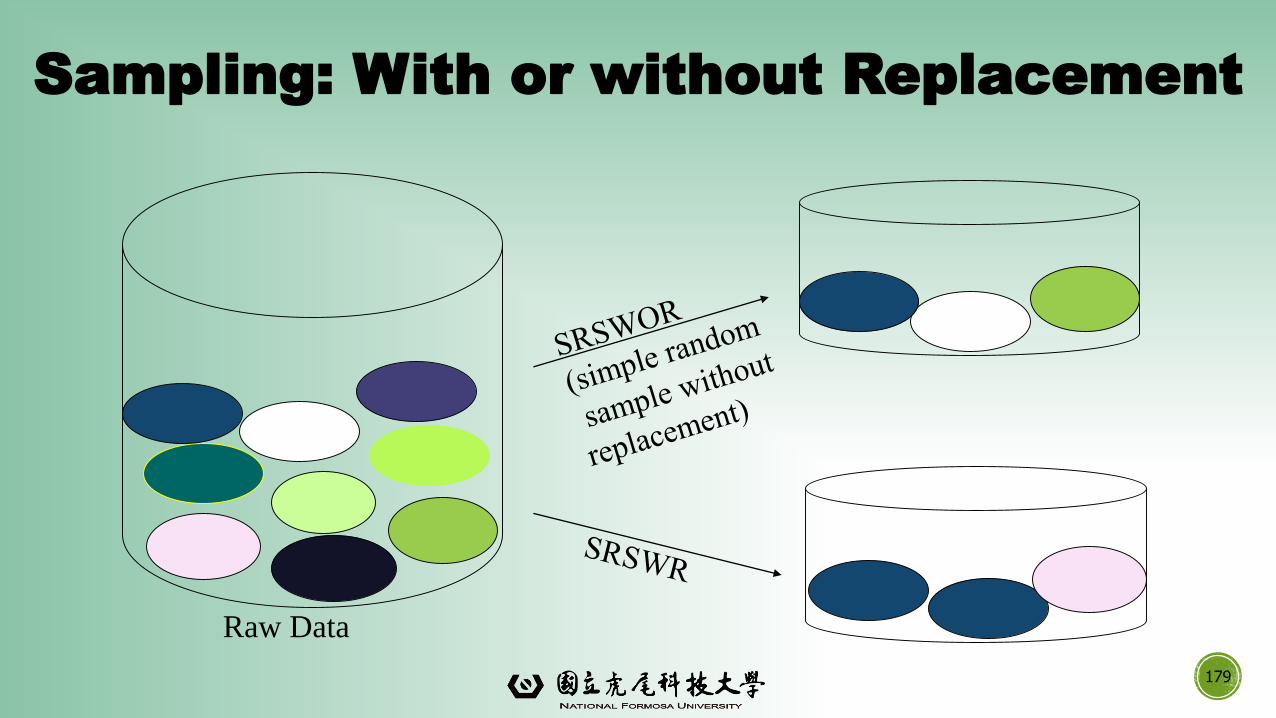
▪Simple random sampling
▪There is an equal probability of selecting any particular item
▪Sampling without replacement
▪Once an object is selected, it is removed from the population
▪Sampling with replacement
▪A selected object is not removed from the population
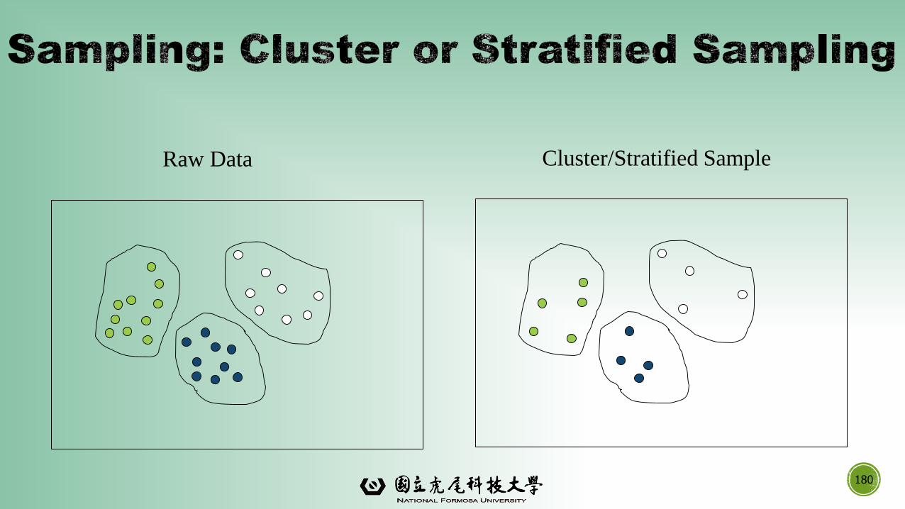
▪Stratified sampling:
▪Partition the data set, and draw samples from each partition (proportionally, i.e., approximately the same percentage of the data)
▪Used in conjunction with skewed data
178
179
Sampling: With or without Replacement
Raw Data
180
Raw Data Cluster/Stratified Sample
181
Data Cube Aggregation
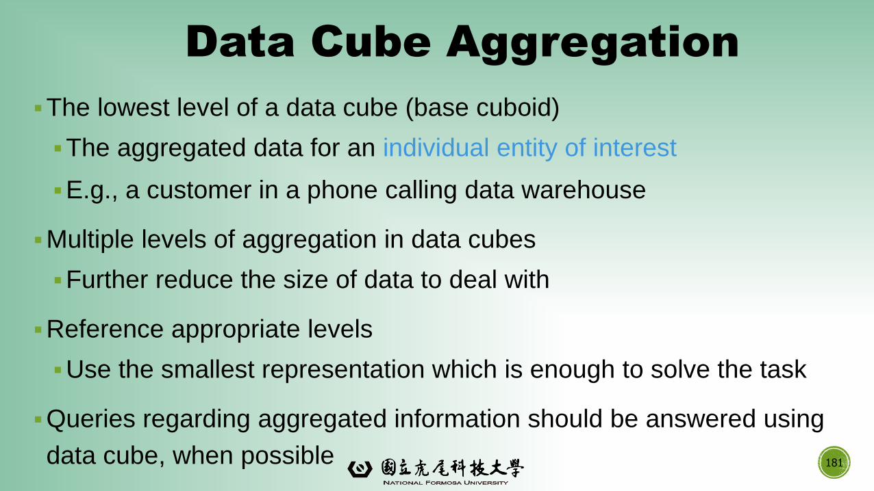
▪The lowest level of a data cube (base cuboid)
▪The aggregated data for an individual entity of interest
▪E.g., a customer in a phone calling data warehouse
▪Multiple levels of aggregation in data cubes
▪Further reduce the size of data to deal with
▪Reference appropriate levels
▪Use the smallest representation which is enough to solve the task
▪Queries regarding aggregated information should be answered using
data cube, when possible
182
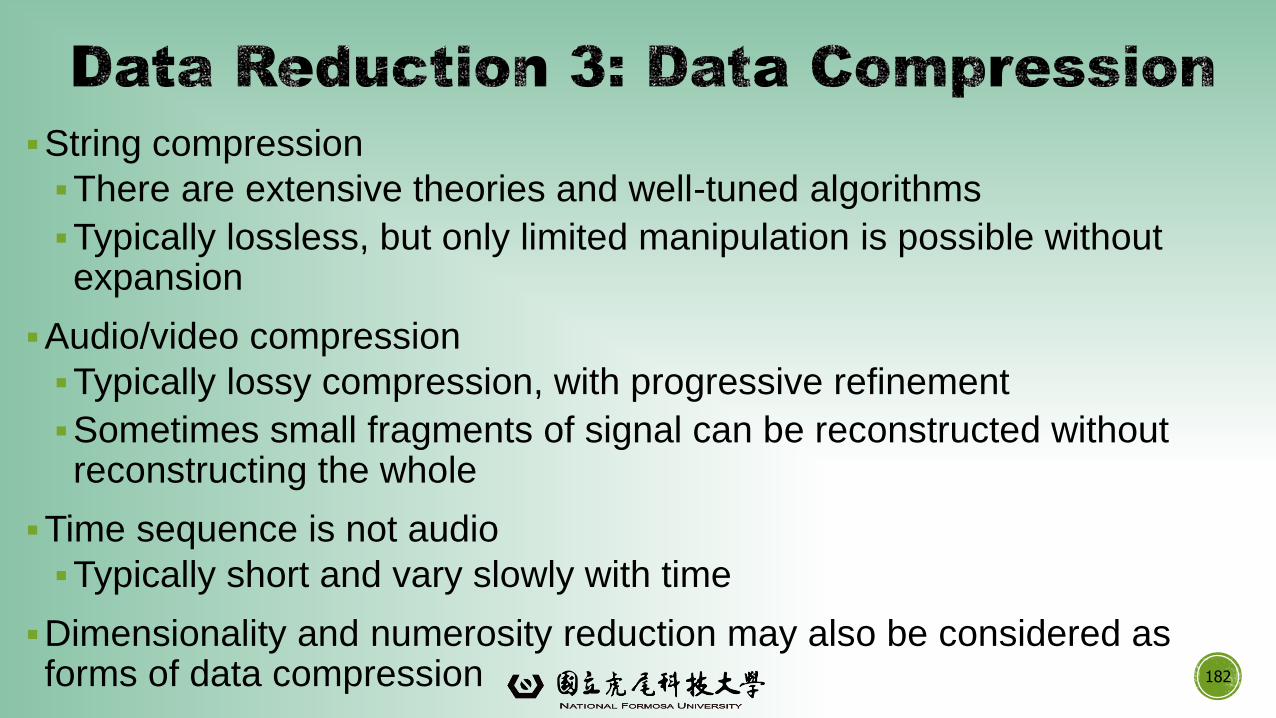
▪String compression
▪There are extensive theories and well-tuned algorithms
▪Typically lossless, but only limited manipulation is possible without expansion
▪Audio/video compression
▪Typically lossy compression, with progressive refinement
▪Sometimes small fragments of signal can be reconstructed without reconstructing the whole
▪Time sequence is not audio
▪Typically short and vary slowly with time
▪Dimensionality and numerosity reduction may also be considered as forms of data compression
183
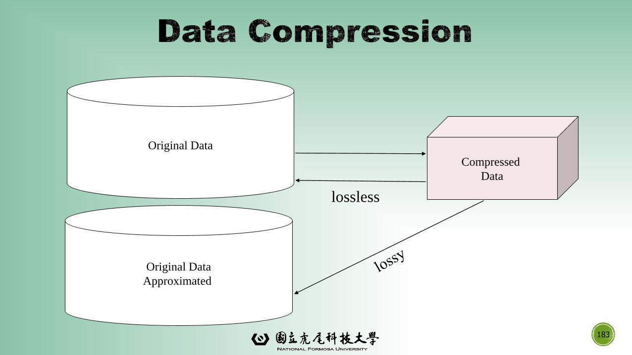
Original Data
Compressed
Data
lossless
Original Data
Approximated

Data Preprocessing: An Overview
➢Data Quality
➢Major Tasks in Data Preprocessing
Data Cleaning
Data Integration
184
Data Reduction
Data Transformation and Data Discretization
Summary
185
186
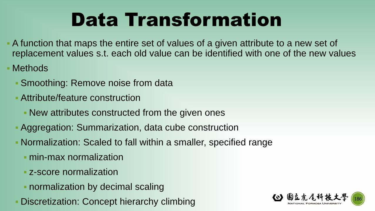
Data Transformation
▪ A function that maps the entire set of values of a given attribute to a new set of replacement values s.t. each old value can be identified with one of the new values
▪Methods
▪ Smoothing: Remove noise from data
▪ Attribute/feature construction
▪New attributes constructed from the given ones
▪ Aggregation: Summarization, data cube construction
▪Normalization: Scaled to fall within a smaller, specified range
▪min-max normalization
▪ z-score normalization
▪ normalization by decimal scaling
▪Discretization: Concept hierarchy climbing
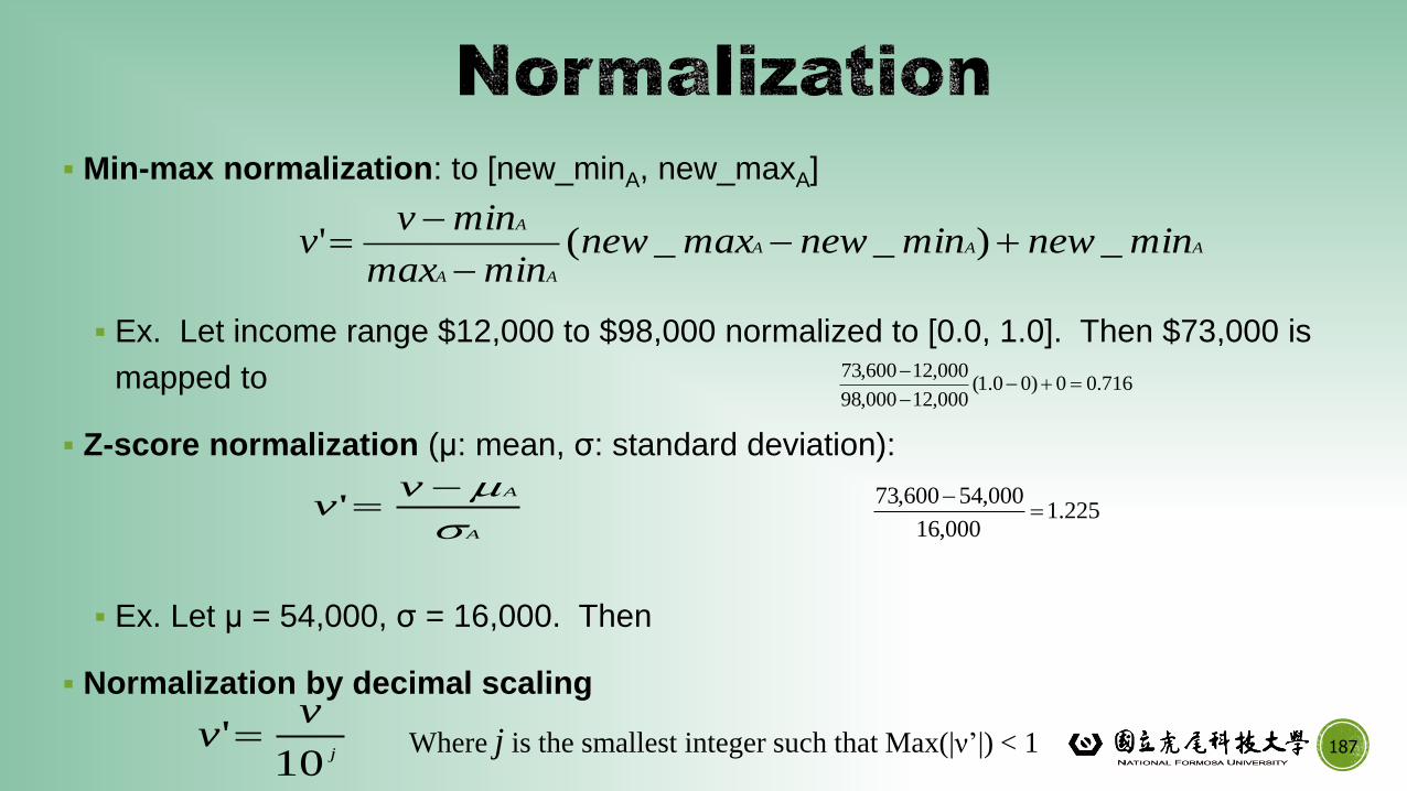
▪ Min-max normalization: to [new_minA, new_maxA]
▪ Ex. Let income range $12,000 to $98,000 normalized to [0.0, 1.0]. Then $73,000 is
mapped to
▪ Z-score normalization (μ: mean, σ: standard deviation):
▪ Ex. Let μ = 54,000, σ = 16,000. Then
▪ Normalization by decimal scaling
716.00)00.1(000,12000,98
000,12600,73
225.1000,16
000,54600,73
187
AAA
AA
A
minnewminnewmaxnewminmax
minvv _)__('
A
Avv
'
j
vv
10' Where j is the smallest integer such that Max(|ν’|) < 1
Discretization
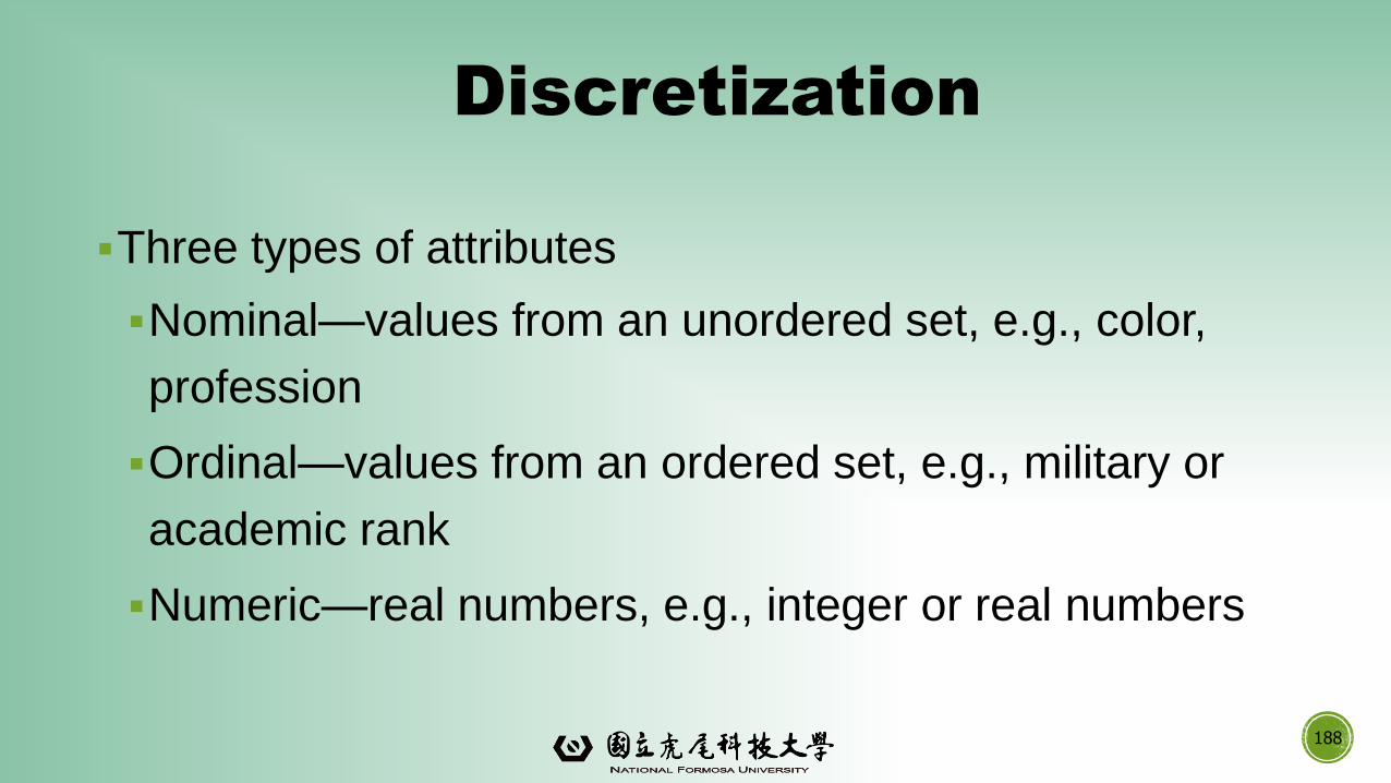
▪Three types of attributes
▪Nominal—values from an unordered set, e.g., color,
profession
▪Ordinal—values from an ordered set, e.g., military or
academic rank
▪Numeric—real numbers, e.g., integer or real numbers
188
Discretization
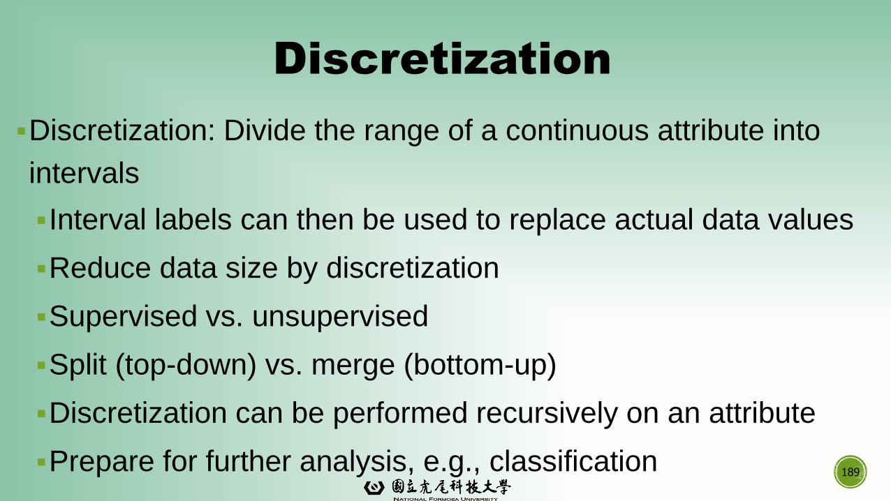
▪Discretization: Divide the range of a continuous attribute into
intervals
▪Interval labels can then be used to replace actual data values
▪Reduce data size by discretization
▪Supervised vs. unsupervised
▪Split (top-down) vs. merge (bottom-up)
▪Discretization can be performed recursively on an attribute
▪Prepare for further analysis, e.g., classification 189
190
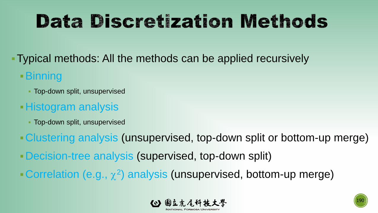
▪Typical methods: All the methods can be applied recursively
▪Binning
▪ Top-down split, unsupervised
▪Histogram analysis
▪ Top-down split, unsupervised
▪Clustering analysis (unsupervised, top-down split or bottom-up merge)
▪Decision-tree analysis (supervised, top-down split)
▪Correlation (e.g., 2) analysis (unsupervised, bottom-up merge)
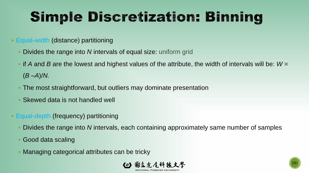
▪ Equal-width (distance) partitioning
▪ Divides the range into N intervals of equal size: uniform grid
▪ if A and B are the lowest and highest values of the attribute, the width of intervals will be: W =
(B –A)/N.
▪ The most straightforward, but outliers may dominate presentation
▪ Skewed data is not handled well
▪ Equal-depth (frequency) partitioning
▪ Divides the range into N intervals, each containing approximately same number of samples
▪ Good data scaling
▪ Managing categorical attributes can be tricky
191
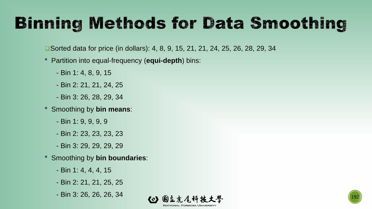
Sorted data for price (in dollars): 4, 8, 9, 15, 21, 21, 24, 25, 26, 28, 29, 34
* Partition into equal-frequency (equi-depth) bins:
- Bin 1: 4, 8, 9, 15
- Bin 2: 21, 21, 24, 25
- Bin 3: 26, 28, 29, 34
* Smoothing by bin means:
- Bin 1: 9, 9, 9, 9
- Bin 2: 23, 23, 23, 23
- Bin 3: 29, 29, 29, 29
* Smoothing by bin boundaries:
- Bin 1: 4, 4, 4, 15
- Bin 2: 21, 21, 25, 25
- Bin 3: 26, 26, 26, 34 192
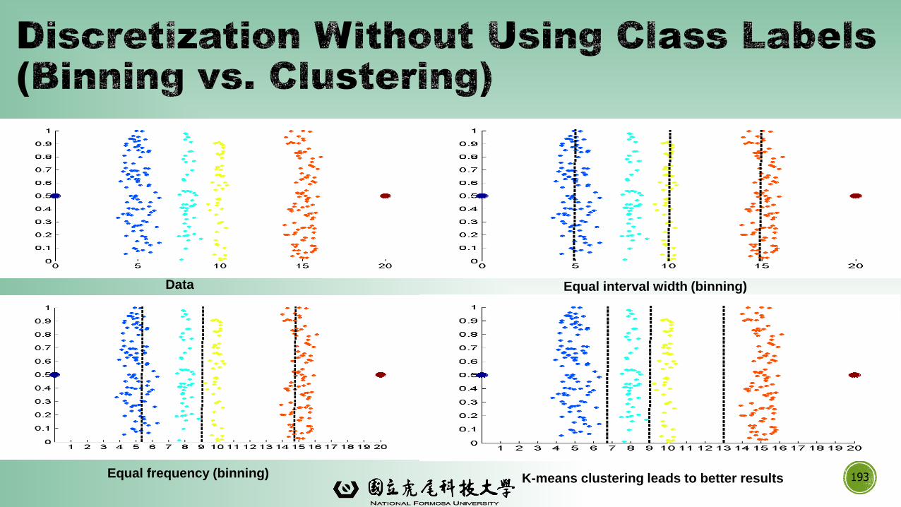
193
Data Equal interval width (binning)
Equal frequency (binning) K-means clustering leads to better results
194
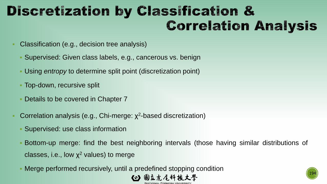
▪ Classification (e.g., decision tree analysis)
▪ Supervised: Given class labels, e.g., cancerous vs. benign
▪ Using entropy to determine split point (discretization point)
▪ Top-down, recursive split
▪ Details to be covered in Chapter 7
▪ Correlation analysis (e.g., Chi-merge: χ2-based discretization)
▪ Supervised: use class information
▪ Bottom-up merge: find the best neighboring intervals (those having similar distributions of
classes, i.e., low χ2 values) to merge
▪ Merge performed recursively, until a predefined stopping condition
Concept Hierarchy Generation
▪ Concept hierarchy organizes concepts (i.e., attribute values) hierarchically and is
usually associated with each dimension in a data warehouse
▪ Concept hierarchies facilitate drilling and rolling in data warehouses to view data in
multiple granularity
▪ Concept hierarchy formation: Recursively reduce the data by collecting and replacing
low level concepts (such as numeric values for age) by higher level concepts (such as
youth, adult, or senior)
▪ Concept hierarchies can be explicitly specified by domain experts and/or data
warehouse designers
▪ Concept hierarchy can be automatically formed for both numeric and nominal data.
For numeric data, use discretization methods shown.195
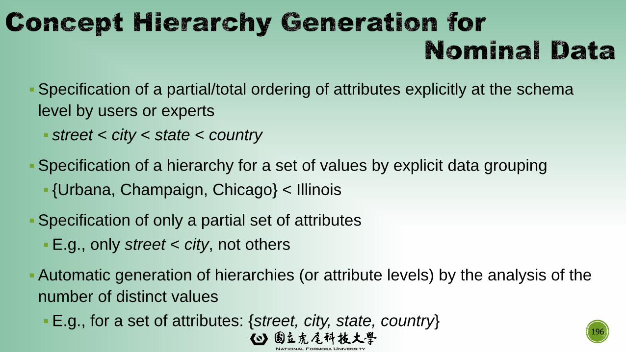
▪Specification of a partial/total ordering of attributes explicitly at the schema
level by users or experts
▪ street < city < state < country
▪Specification of a hierarchy for a set of values by explicit data grouping
▪ {Urbana, Champaign, Chicago} < Illinois
▪Specification of only a partial set of attributes
▪E.g., only street < city, not others
▪Automatic generation of hierarchies (or attribute levels) by the analysis of the
number of distinct values
▪E.g., for a set of attributes: {street, city, state, country}196
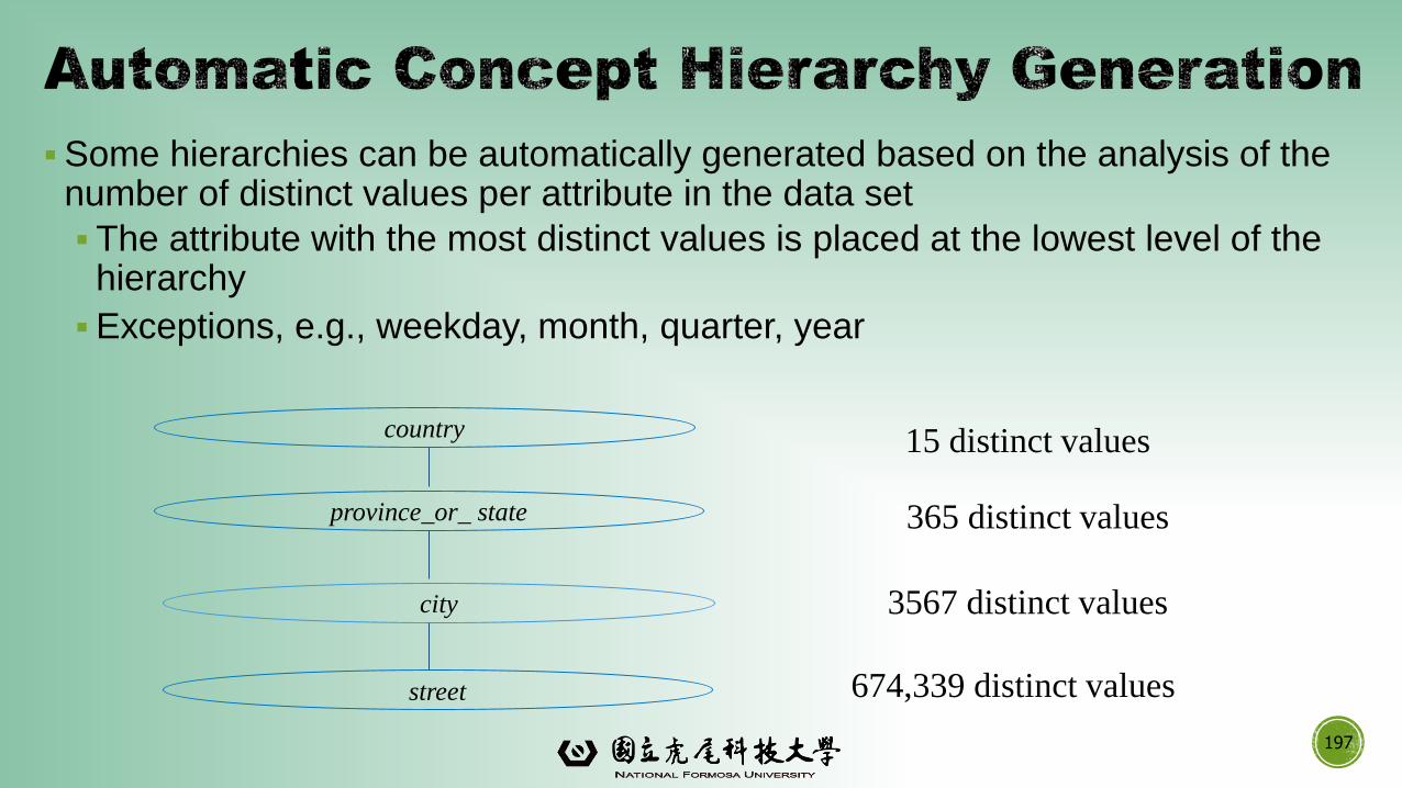
▪Some hierarchies can be automatically generated based on the analysis of the number of distinct values per attribute in the data set
▪ The attribute with the most distinct values is placed at the lowest level of the hierarchy
▪Exceptions, e.g., weekday, month, quarter, year
197
country
province_or_ state
city
street
15 distinct values
365 distinct values
3567 distinct values
674,339 distinct values

Data Preprocessing: An Overview
➢Data Quality
➢Major Tasks in Data Preprocessing
Data Cleaning
Data Integration
198
Data Reduction
Data Transformation and Data Discretization
Summary
199
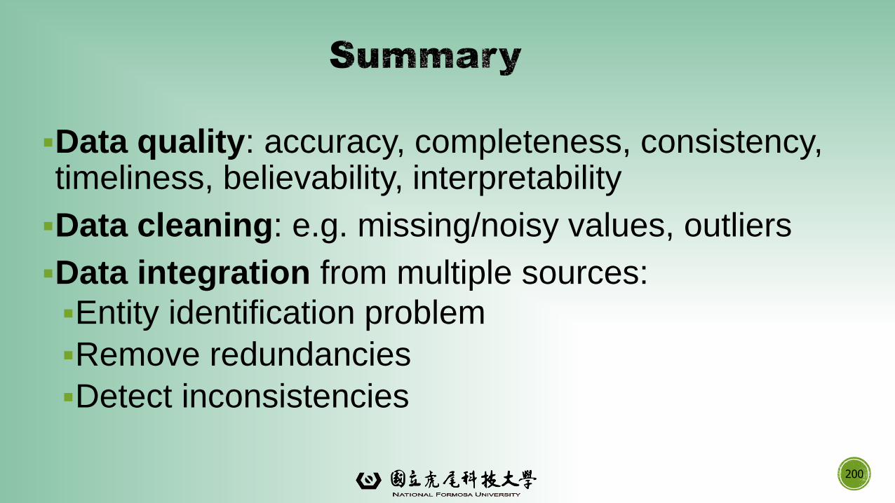
▪Data quality: accuracy, completeness, consistency, timeliness, believability, interpretability
▪Data cleaning: e.g. missing/noisy values, outliers
▪Data integration from multiple sources:
▪Entity identification problem
▪Remove redundancies
▪Detect inconsistencies
200
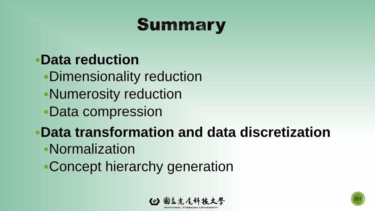
▪Data reduction
▪Dimensionality reduction
▪Numerosity reduction
▪Data compression
▪Data transformation and data discretization
▪Normalization
▪Concept hierarchy generation
201
▪ D. P. Ballou and G. K. Tayi. Enhancing data quality in data warehouse environments. Comm. of ACM, 42:73-78, 1999
▪ A. Bruce, D. Donoho, and H.-Y. Gao. Wavelet analysis. IEEE Spectrum, Oct 1996
▪ T. Dasu and T. Johnson. Exploratory Data Mining and Data Cleaning. John Wiley, 2003
▪ J. Devore and R. Peck. Statistics: The Exploration and Analysis of Data. Duxbury Press, 1997.
▪ H. Galhardas, D. Florescu, D. Shasha, E. Simon, and C.-A. Saita. Declarative data cleaning: Language, model, and algorithms. VLDB'01
▪ M. Hua and J. Pei. Cleaning disguised missing data: A heuristic approach. KDD'07
202
▪ H. V. Jagadish, et al., Special Issue on Data Reduction Techniques. Bulletin of the Technical Committee on Data Engineering, 20(4), Dec. 1997
▪ H. Liu and H. Motoda (eds.). Feature Extraction, Construction, and Selection: A Data Mining Perspective. Kluwer Academic, 1998
▪ J. E. Olson. Data Quality: The Accuracy Dimension. Morgan Kaufmann, 2003
▪ D. Pyle. Data Preparation for Data Mining. Morgan Kaufmann, 1999
▪ V. Raman and J. Hellerstein. Potters Wheel: An Interactive Framework for Data Cleaning and Transformation, VLDB’2001
▪ T. Redman. Data Quality: The Field Guide. Digital Press (Elsevier), 2001
▪ R. Wang, V. Storey, and C. Firth. A framework for analysis of data quality research. IEEE Trans. Knowledge and Data Engineering, 7:623-640, 1995
203

Data Warehouse: Basic Concepts
Data Warehouse Modeling: Data Cube and OLAP
Data Warehouse Design and Usage
Data Warehouse Implementation
Data Generalization by Attribute-Oriented Induction
Summary204
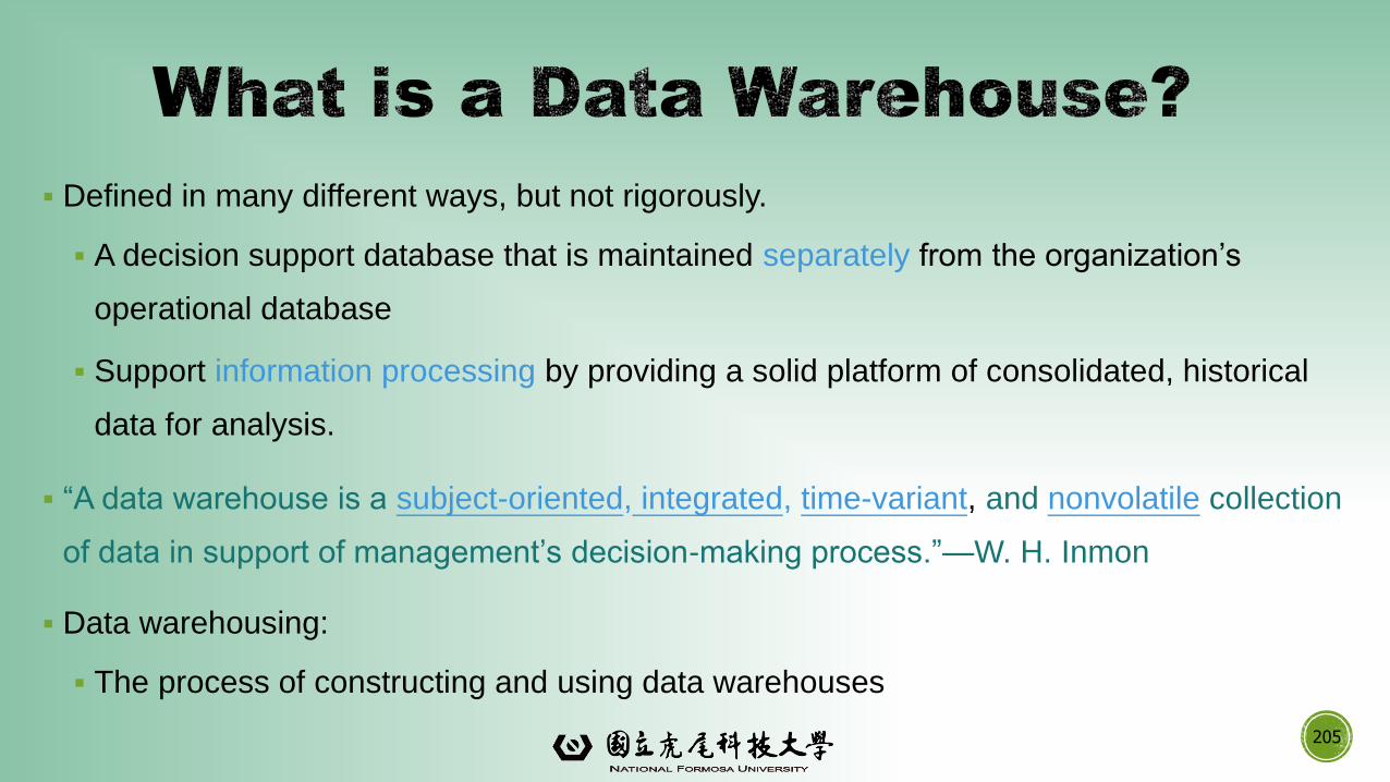
▪ Defined in many different ways, but not rigorously.
▪ A decision support database that is maintained separately from the organization’s
operational database
▪ Support information processing by providing a solid platform of consolidated, historical
data for analysis.
▪ “A data warehouse is a subject-oriented, integrated, time-variant, and nonvolatile collection
of data in support of management’s decision-making process.”—W. H. Inmon
▪ Data warehousing:
▪ The process of constructing and using data warehouses
205
▪Organized around major subjects, such as customer, product, sales
▪Focusing on the modeling and analysis of data for decision makers,
not on daily operations or transaction processing
▪Provide a simple and concise view around particular subject issues
by excluding data that are not useful in the decision support
process
206
▪Constructed by integrating multiple, heterogeneous data sources
▪ relational databases, flat files, on-line transaction records
▪Data cleaning and data integration techniques are applied.
▪Ensure consistency in naming conventions, encoding structures, attribute measures, etc. among different data sources
▪ E.g., Hotel price: currency, tax, breakfast covered, etc.
▪When data is moved to the warehouse, it is converted.
207
▪ The time horizon for the data warehouse is significantly longer than that of
operational systems
▪Operational database: current value data
▪Data warehouse data: provide information from a historical perspective (e.g.,
past 5-10 years)
▪ Every key structure in the data warehouse
▪Contains an element of time, explicitly or implicitly
▪ But the key of operational data may or may not contain “time element”
208
▪A physically separate store of data transformed from the
operational environment
▪Operational update of data does not occur in the data warehouse
environment
▪Does not require transaction processing, recovery, and
concurrency control mechanisms
▪Requires only two operations in data accessing:
▪ initial loading of data and access of data
209
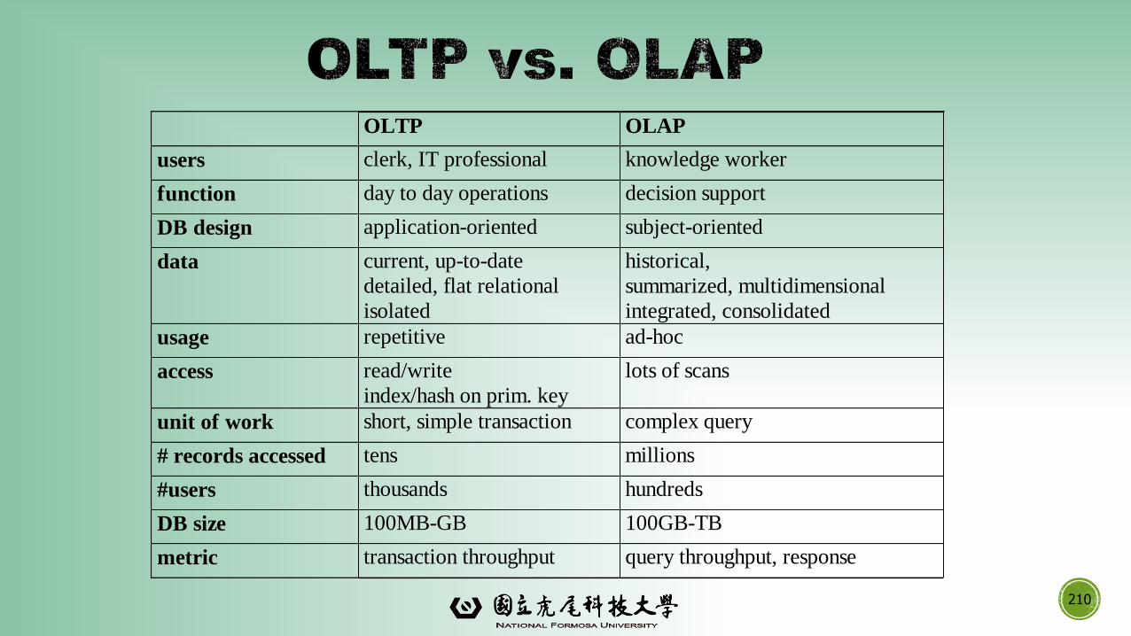
OLTP OLAP
users clerk, IT professional knowledge worker
function day to day operations decision support
DB design application-oriented subject-oriented
data current, up-to-date
detailed, flat relational
isolated
historical,
summarized, multidimensional
integrated, consolidated
usage repetitive ad-hoc
access read/write
index/hash on prim. key
lots of scans
unit of work short, simple transaction complex query
# records accessed tens millions
#users thousands hundreds
DB size 100MB-GB 100GB-TB
metric transaction throughput query throughput, response
210
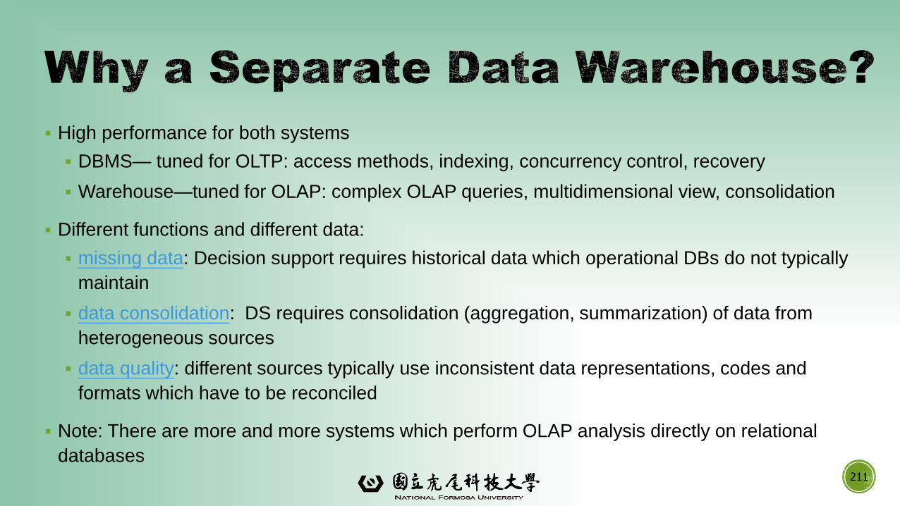
▪ High performance for both systems
▪ DBMS— tuned for OLTP: access methods, indexing, concurrency control, recovery
▪ Warehouse—tuned for OLAP: complex OLAP queries, multidimensional view, consolidation
▪ Different functions and different data:
▪ missing data: Decision support requires historical data which operational DBs do not typically
maintain
▪ data consolidation: DS requires consolidation (aggregation, summarization) of data from
heterogeneous sources
▪ data quality: different sources typically use inconsistent data representations, codes and
formats which have to be reconciled
▪ Note: There are more and more systems which perform OLAP analysis directly on relational
databases211
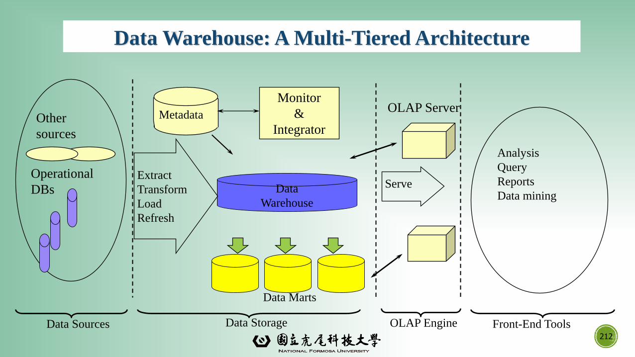
212
Data Warehouse: A Multi-Tiered Architecture
Data
Warehouse
Extract
Transform
Load
Refresh
OLAP Engine
Analysis
Query
Reports
Data mining
Monitor
&
Integrator
Metadata
Data Sources Front-End Tools
Serve
Data Marts
Operational
DBs
Other
sources
Data Storage
OLAP Server
▪ Enterprise warehouse
▪ collects all of the information about subjects spanning the entire organization
▪Data Mart
▪ a subset of corporate-wide data that is of value to a specific groups of users.
Its scope is confined to specific, selected groups, such as marketing data
mart
▪ Independent vs. dependent (directly from warehouse) data mart
▪ Virtual warehouse
▪ A set of views over operational databases
▪Only some of the possible summary views may be materialized
213
▪Data extraction
▪ get data from multiple, heterogeneous, and external sources
▪Data cleaning
▪ detect errors in the data and rectify them when possible
▪Data transformation
▪ convert data from legacy or host format to warehouse format
▪ Load
▪ sort, summarize, consolidate, compute views, check integrity, and build indicies and partitions
▪Refresh
▪ propagate the updates from the data sources to the warehouse
214
▪ Meta data is the data defining warehouse objects. It stores:
▪ Description of the structure of the data warehouse
▪ schema, view, dimensions, hierarchies, derived data defn, data mart locations and contents
▪ Operational meta-data
▪ data lineage (history of migrated data and transformation path), currency of data (active, archived,
or purged), monitoring information (warehouse usage statistics, error reports, audit trails)
▪ The algorithms used for summarization
▪ The mapping from operational environment to the data warehouse
▪ Data related to system performance
▪ warehouse schema, view and derived data definitions
▪ Business data
▪ business terms and definitions, ownership of data, charging policies215
Data Warehouse: Basic Concepts
Data Warehouse Modeling: Data Cube and OLAP
Data Warehouse Design and Usage
Data Warehouse Implementation
Data Generalization by Attribute-Oriented Induction
Summary216
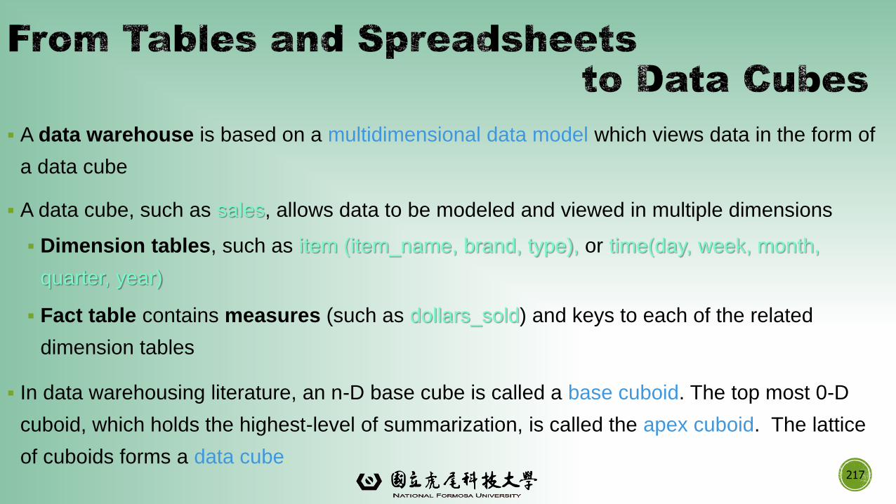
▪ A data warehouse is based on a multidimensional data model which views data in the form of
a data cube
▪ A data cube, such as sales, allows data to be modeled and viewed in multiple dimensions
▪ Dimension tables, such as item (item_name, brand, type), or time(day, week, month,
quarter, year)
▪ Fact table contains measures (such as dollars_sold) and keys to each of the related
dimension tables
▪ In data warehousing literature, an n-D base cube is called a base cuboid. The top most 0-D
cuboid, which holds the highest-level of summarization, is called the apex cuboid. The lattice
of cuboids forms a data cube.217
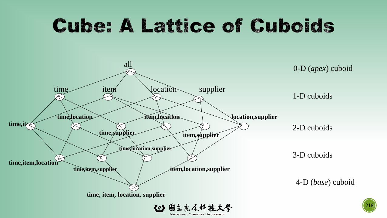
218
time,item
time,item,location
time, item, location, supplier
all
time item location supplier
time,location
time,supplier
item,location
item,supplier
location,supplier
time,item,supplier
time,location,supplier
item,location,supplier
0-D (apex) cuboid
1-D cuboids
2-D cuboids
3-D cuboids
4-D (base) cuboid
▪Modeling data warehouses: dimensions & measures
▪Star schema: A fact table in the middle connected to a set of
dimension tables
▪Snowflake schema: A refinement of star schema where some
dimensional hierarchy is normalized into a set of smaller
dimension tables, forming a shape similar to snowflake
▪Fact constellations: Multiple fact tables share dimension tables,
viewed as a collection of stars, therefore called galaxy schema or
fact constellation219
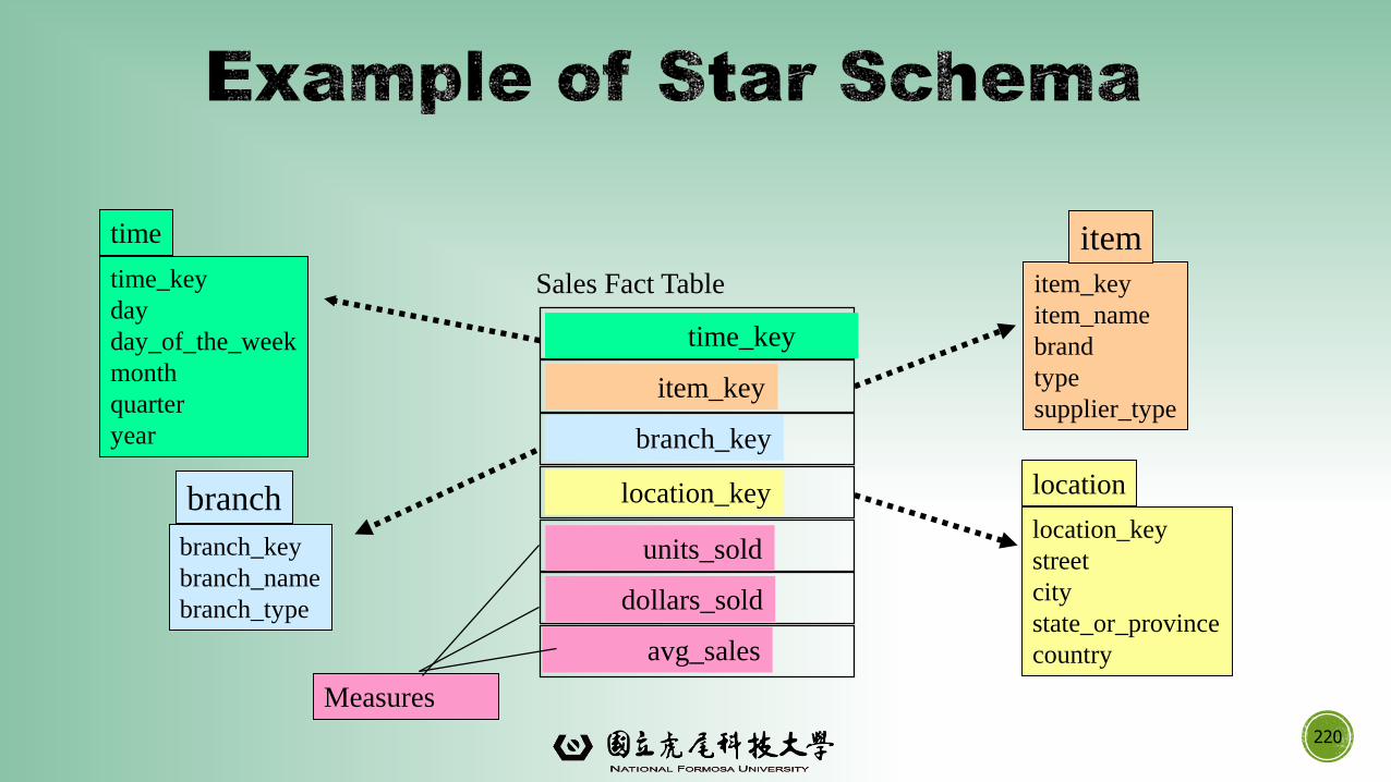
220
time_key
day
day_of_the_week
month
quarter
year
time
location_key
street
city
state_or_province
country
location
Sales Fact Table
time_key
item_key
branch_key
location_key
units_sold
dollars_sold
avg_sales
Measures
item_key
item_name
brand
type
supplier_type
item
branch_key
branch_name
branch_type
branch
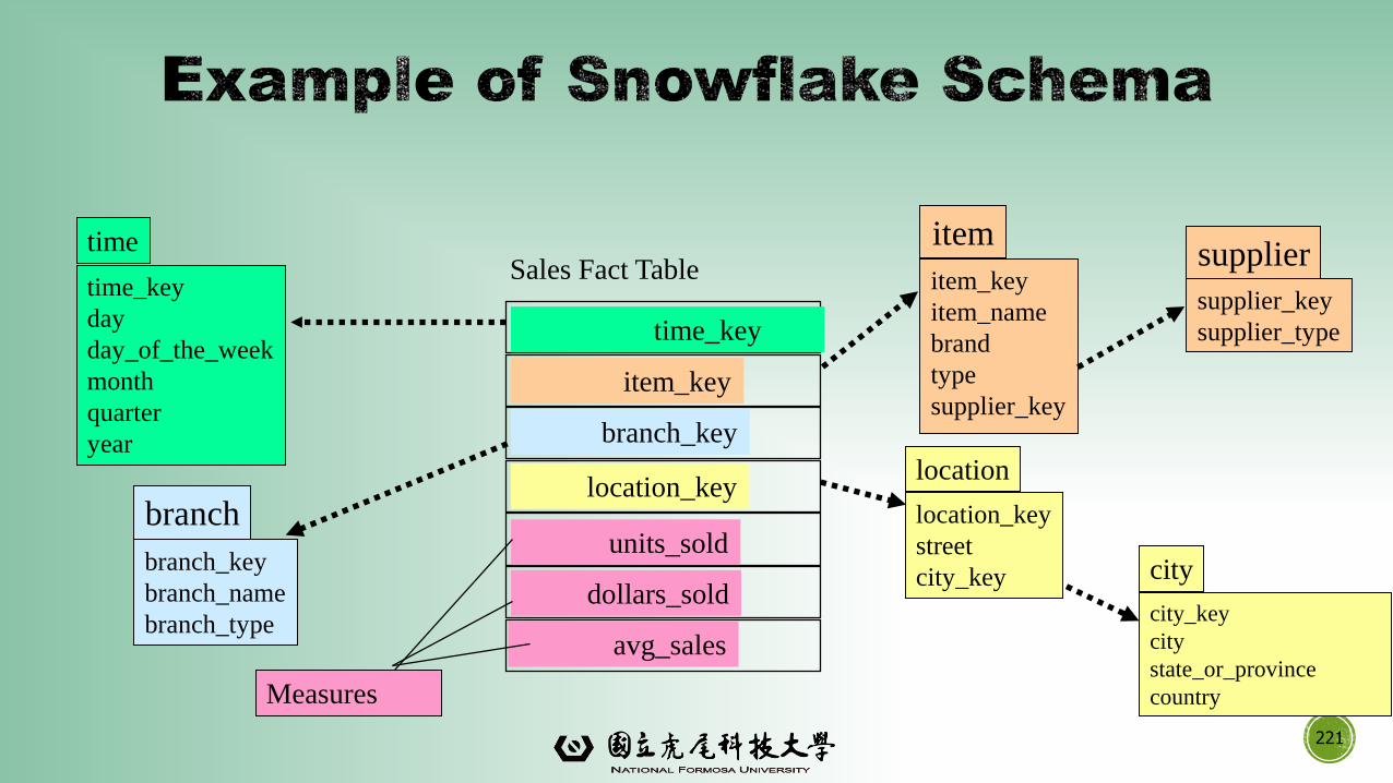
221
time_key
day
day_of_the_week
month
quarter
year
time
location_key
street
city_key
location
Sales Fact Table
time_key
item_key
branch_key
location_key
units_sold
dollars_sold
avg_sales
Measures
item_key
item_name
brand
type
supplier_key
item
branch_key
branch_name
branch_type
branch
supplier_key
supplier_type
supplier
city_key
city
state_or_province
country
city
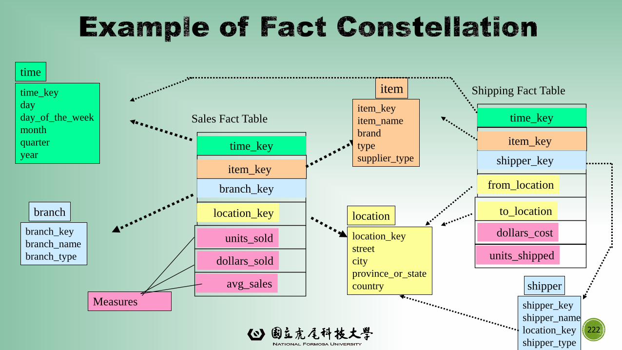
222
time_key
day
day_of_the_week
month
quarter
year
time
location_key
street
city
province_or_state
country
location
Sales Fact Table
time_key
item_key
branch_key
location_key
units_sold
dollars_sold
avg_sales
Measures
item_key
item_name
brand
type
supplier_type
item
branch_key
branch_name
branch_type
branch
Shipping Fact Table
time_key
item_key
shipper_key
from_location
to_location
dollars_cost
units_shipped
shipper_key
shipper_name
location_key
shipper_type
shipper
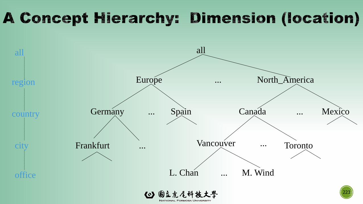
223
all
Europe North_America
MexicoCanadaSpainGermany
Vancouver
M. WindL. Chan
...
......
... ...
...
all
region
office
country
TorontoFrankfurtcity
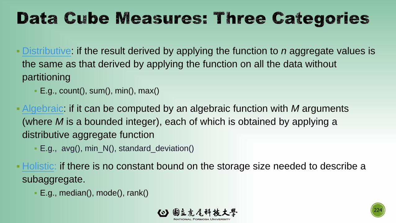
▪Distributive: if the result derived by applying the function to n aggregate values is
the same as that derived by applying the function on all the data without
partitioning
▪ E.g., count(), sum(), min(), max()
▪ Algebraic: if it can be computed by an algebraic function with M arguments
(where M is a bounded integer), each of which is obtained by applying a
distributive aggregate function
▪ E.g., avg(), min_N(), standard_deviation()
▪Holistic: if there is no constant bound on the storage size needed to describe a
subaggregate.
▪ E.g., median(), mode(), rank()
224
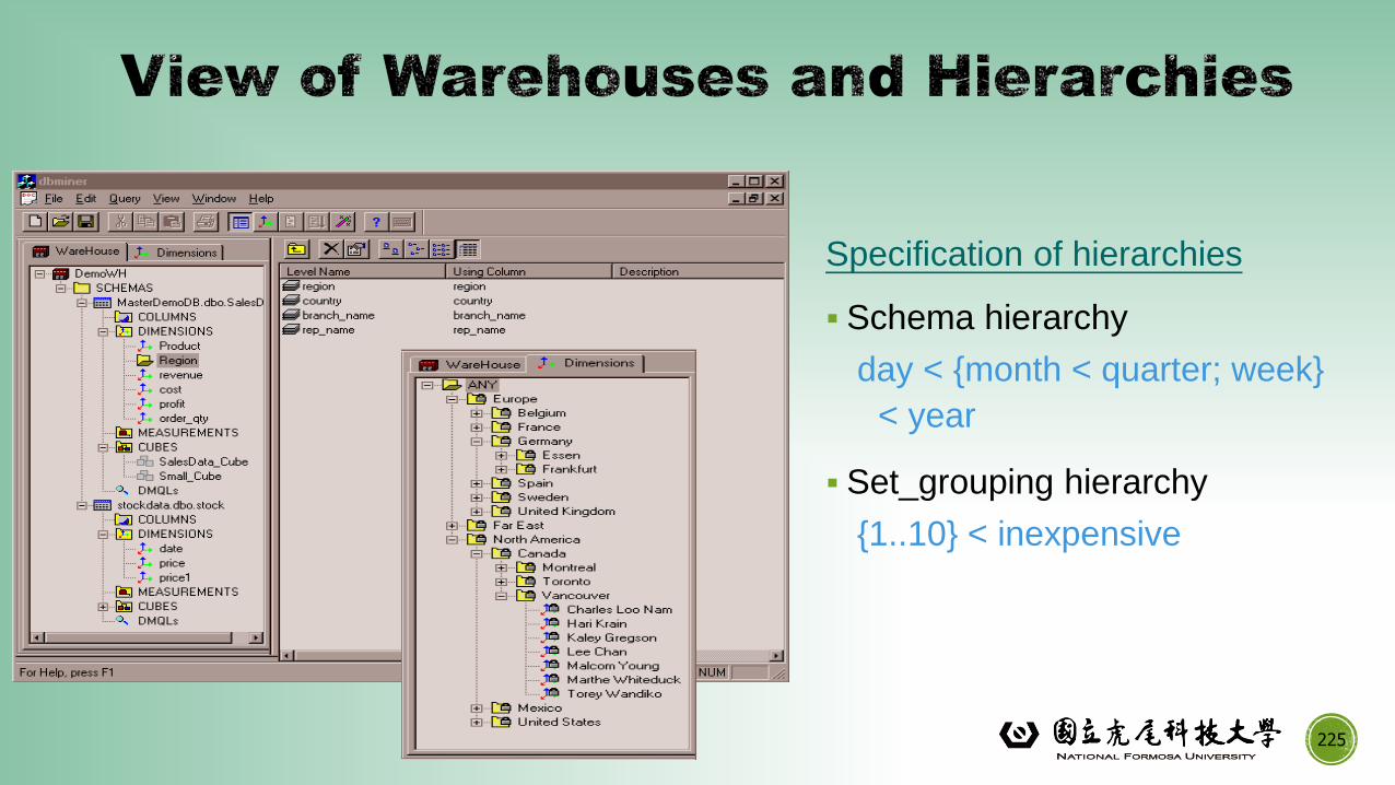
Specification of hierarchies
▪ Schema hierarchy
day < {month < quarter; week}
< year
▪ Set_grouping hierarchy
{1..10} < inexpensive
225

▪ Sales volume as a function of product, month, and region
226
Pro
duct
Month
Dimensions: Product, Location, Time
Hierarchical summarization paths
Industry Region Year
Category Country Quarter
Product City Month Week
Office Day
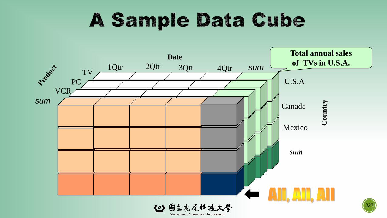
227
Total annual sales
of TVs in U.S.A.Date
Cou
ntr
ysum
sumTV
VCRPC
1Qtr 2Qtr 3Qtr 4Qtr
U.S.A
Canada
Mexico
sum
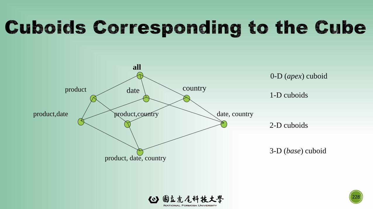
228
all
product date country
product,date product,country date, country
product, date, country
0-D (apex) cuboid
1-D cuboids
2-D cuboids
3-D (base) cuboid
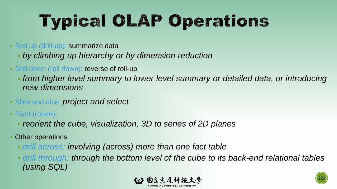
▪ Roll up (drill-up): summarize data
▪ by climbing up hierarchy or by dimension reduction
▪ Drill down (roll down): reverse of roll-up
▪ from higher level summary to lower level summary or detailed data, or introducing new dimensions
▪ Slice and dice: project and select
▪ Pivot (rotate):
▪ reorient the cube, visualization, 3D to series of 2D planes
▪ Other operations
▪ drill across: involving (across) more than one fact table
▪ drill through: through the bottom level of the cube to its back-end relational tables (using SQL)
229
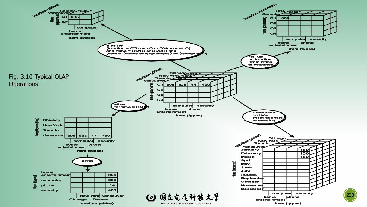
230
Fig. 3.10 Typical OLAP Operations
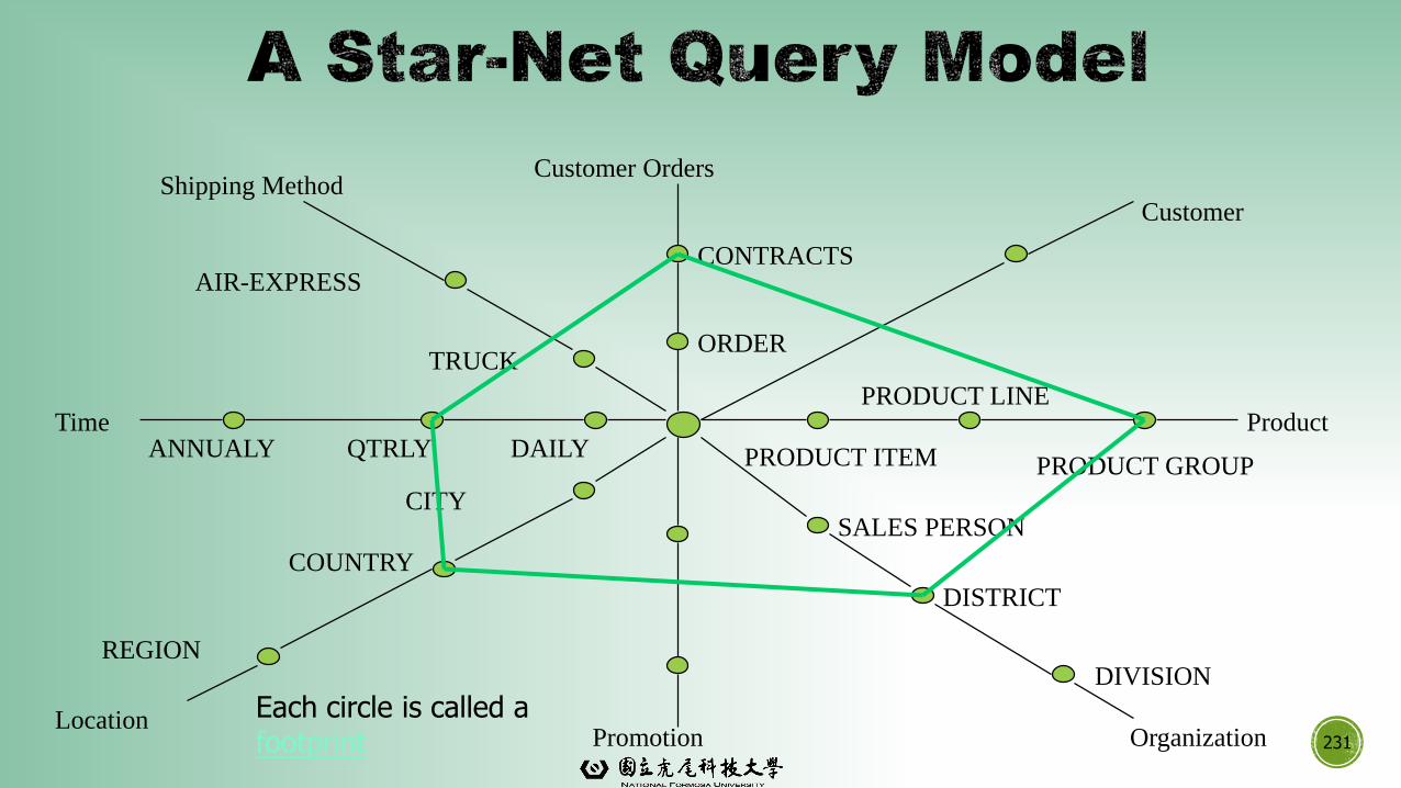
231
Shipping Method
AIR-EXPRESS
TRUCKORDER
Customer Orders
CONTRACTS
Customer
Product
PRODUCT GROUP
PRODUCT LINE
PRODUCT ITEM
SALES PERSON
DISTRICT
DIVISION
OrganizationPromotion
CITY
COUNTRY
REGION
Location
DAILYQTRLYANNUALYTime
Each circle is called a footprint
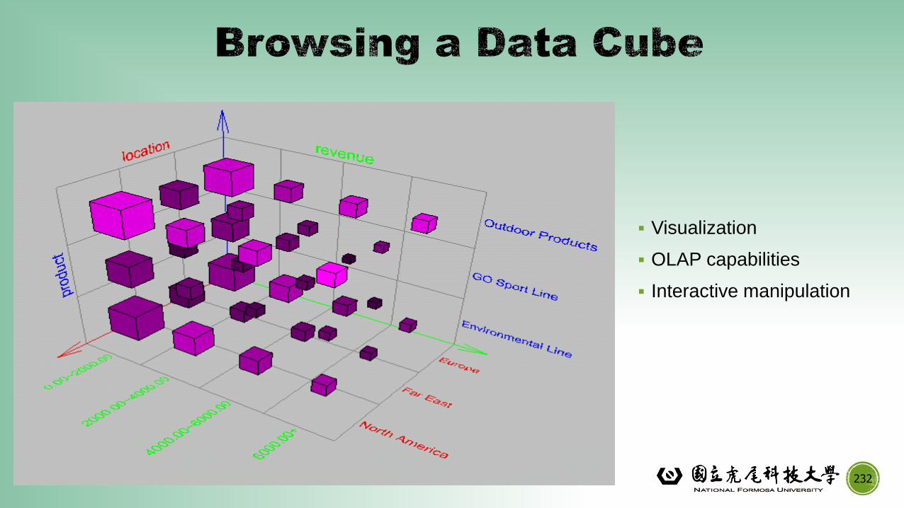
▪ Visualization
▪ OLAP capabilities
▪ Interactive manipulation
232
Data Warehouse: Basic Concepts
Data Warehouse Modeling: Data Cube and OLAP
Data Warehouse Design and Usage
Data Warehouse Implementation
Data Generalization by Attribute-Oriented Induction
Summary233
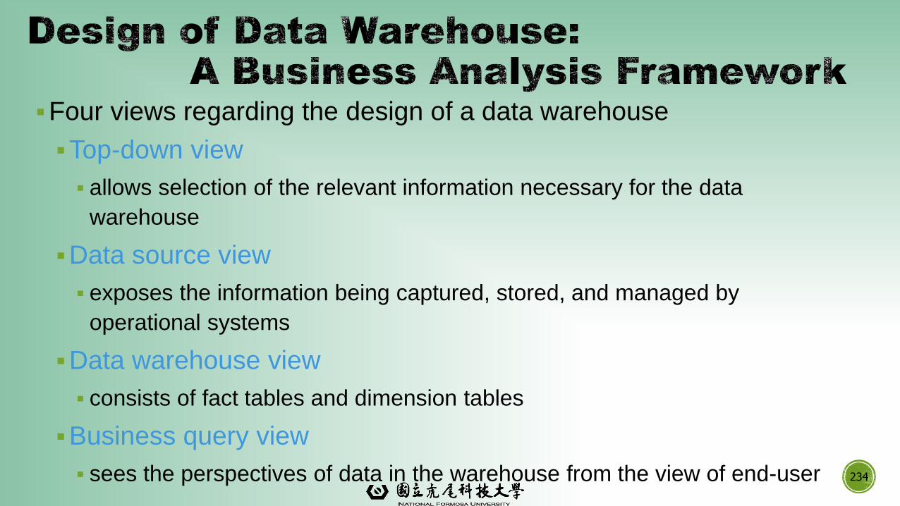
▪Four views regarding the design of a data warehouse
▪Top-down view
▪ allows selection of the relevant information necessary for the data
warehouse
▪Data source view
▪ exposes the information being captured, stored, and managed by
operational systems
▪Data warehouse view
▪ consists of fact tables and dimension tables
▪Business query view
▪ sees the perspectives of data in the warehouse from the view of end-user 234
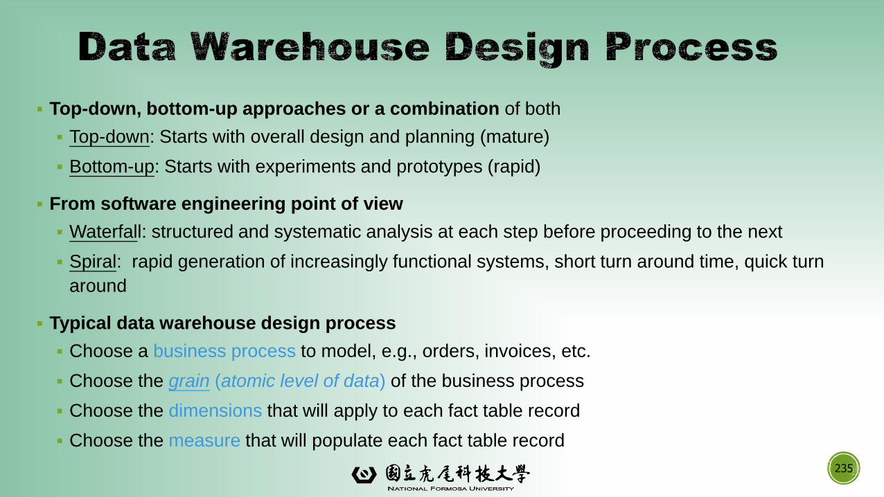
▪ Top-down, bottom-up approaches or a combination of both
▪ Top-down: Starts with overall design and planning (mature)
▪ Bottom-up: Starts with experiments and prototypes (rapid)
▪ From software engineering point of view
▪ Waterfall: structured and systematic analysis at each step before proceeding to the next
▪ Spiral: rapid generation of increasingly functional systems, short turn around time, quick turn
around
▪ Typical data warehouse design process
▪ Choose a business process to model, e.g., orders, invoices, etc.
▪ Choose the grain (atomic level of data) of the business process
▪ Choose the dimensions that will apply to each fact table record
▪ Choose the measure that will populate each fact table record
235
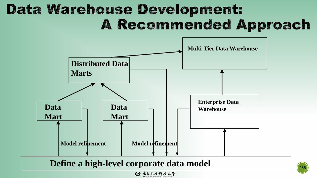
236Define a high-level corporate data model
Data
Mart
Data
Mart
Distributed Data
Marts
Multi-Tier Data Warehouse
Enterprise Data
Warehouse
Model refinementModel refinement
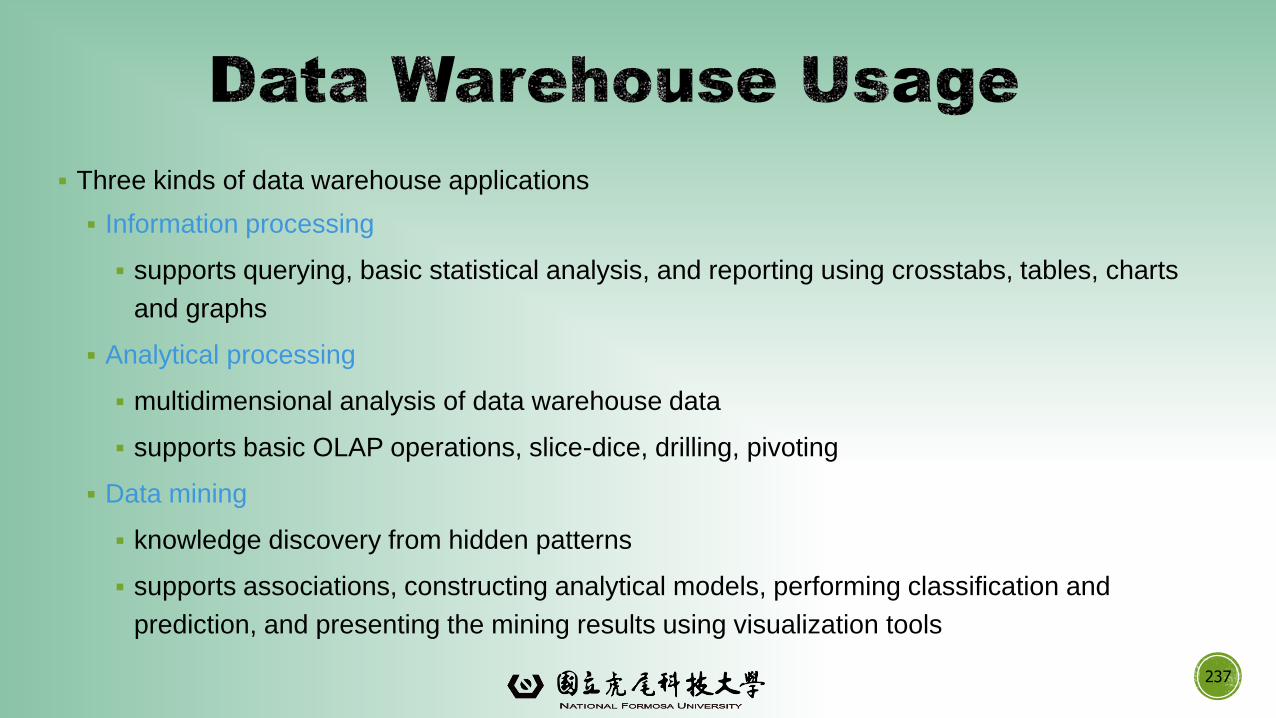
▪ Three kinds of data warehouse applications
▪ Information processing
▪ supports querying, basic statistical analysis, and reporting using crosstabs, tables, charts
and graphs
▪ Analytical processing
▪ multidimensional analysis of data warehouse data
▪ supports basic OLAP operations, slice-dice, drilling, pivoting
▪ Data mining
▪ knowledge discovery from hidden patterns
▪ supports associations, constructing analytical models, performing classification and
prediction, and presenting the mining results using visualization tools
237
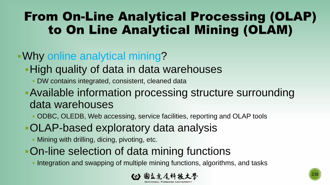
From On-Line Analytical Processing (OLAP)
to On Line Analytical Mining (OLAM)
▪Why online analytical mining?
▪High quality of data in data warehouses▪ DW contains integrated, consistent, cleaned data
▪Available information processing structure surrounding data warehouses▪ ODBC, OLEDB, Web accessing, service facilities, reporting and OLAP tools
▪OLAP-based exploratory data analysis▪ Mining with drilling, dicing, pivoting, etc.
▪On-line selection of data mining functions▪ Integration and swapping of multiple mining functions, algorithms, and tasks
238
Data Warehouse: Basic Concepts
Data Warehouse Modeling: Data Cube and OLAP
Data Warehouse Design and Usage
Data Warehouse Implementation
Data Generalization by Attribute-Oriented Induction
Summary239
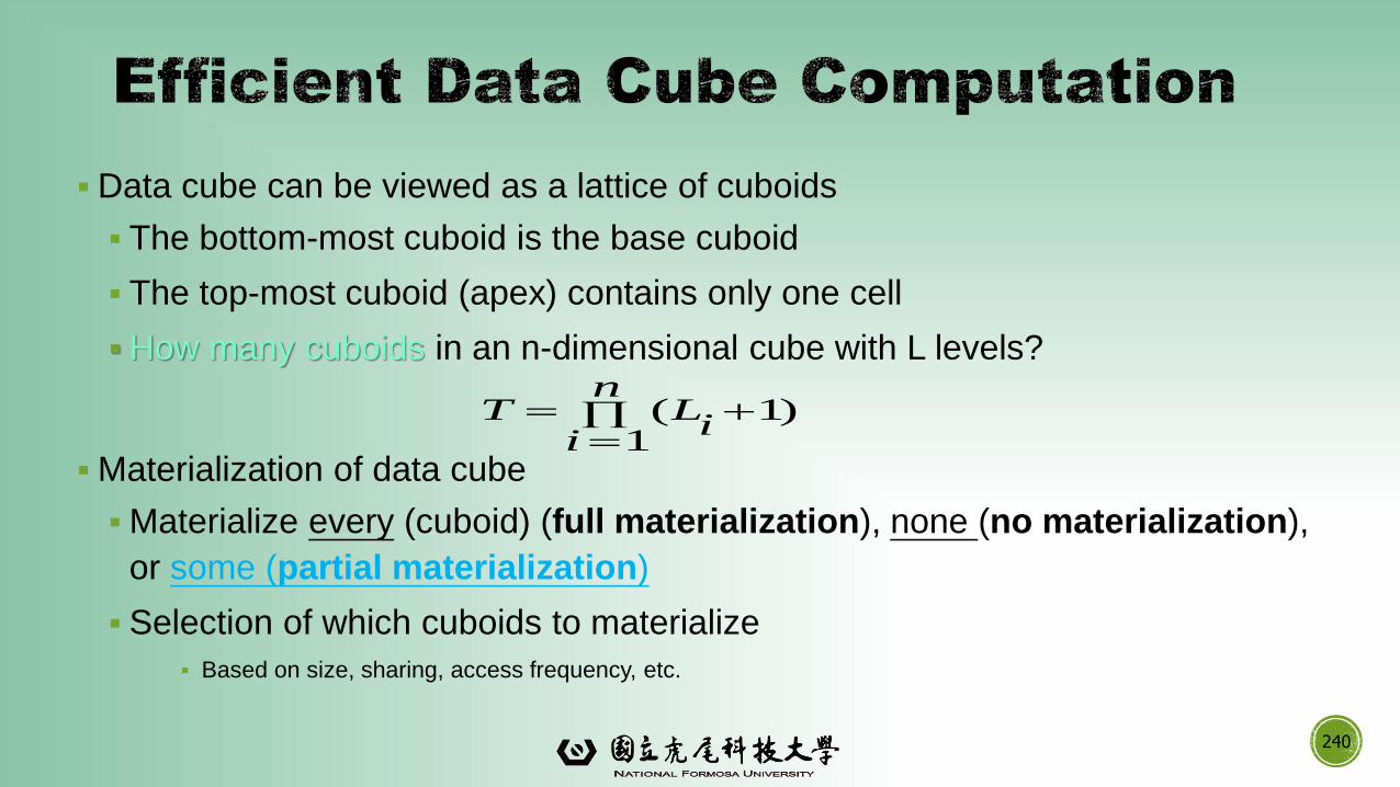
▪Data cube can be viewed as a lattice of cuboids
▪ The bottom-most cuboid is the base cuboid
▪ The top-most cuboid (apex) contains only one cell
▪How many cuboids in an n-dimensional cube with L levels?
▪Materialization of data cube
▪Materialize every (cuboid) (full materialization), none (no materialization),
or some (partial materialization)
▪ Selection of which cuboids to materialize
▪ Based on size, sharing, access frequency, etc.
240
)11(
n
ii
LT
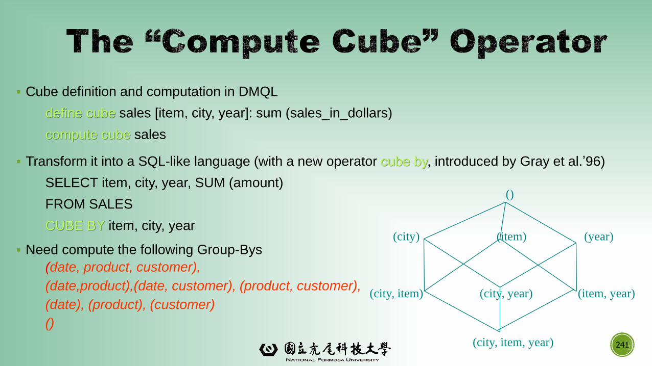
▪ Cube definition and computation in DMQL
define cube sales [item, city, year]: sum (sales_in_dollars)
compute cube sales
▪ Transform it into a SQL-like language (with a new operator cube by, introduced by Gray et al.’96)
SELECT item, city, year, SUM (amount)
FROM SALES
CUBE BY item, city, year
▪ Need compute the following Group-Bys
(date, product, customer),
(date,product),(date, customer), (product, customer),
(date), (product), (customer)
()
241
(item)(city)
()
(year)
(city, item) (city, year) (item, year)
(city, item, year)
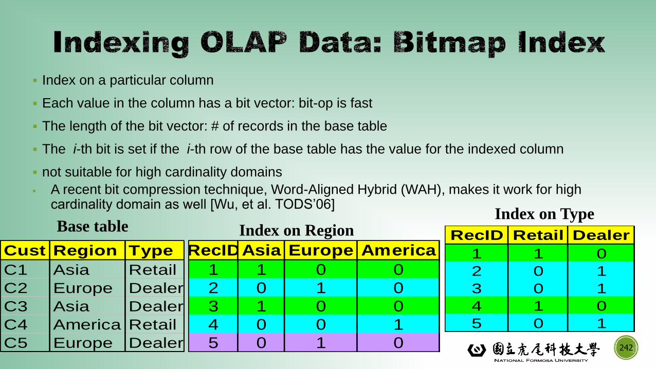
▪ Index on a particular column
▪ Each value in the column has a bit vector: bit-op is fast
▪ The length of the bit vector: # of records in the base table
▪ The i-th bit is set if the i-th row of the base table has the value for the indexed column
▪ not suitable for high cardinality domains
▪ A recent bit compression technique, Word-Aligned Hybrid (WAH), makes it work for high cardinality domain as well [Wu, et al. TODS’06]
242
Cust Region Type
C1 Asia Retail
C2 Europe Dealer
C3 Asia Dealer
C4 America Retail
C5 Europe Dealer
RecID Retail Dealer
1 1 0
2 0 1
3 0 1
4 1 0
5 0 1
RecIDAsia Europe America
1 1 0 0
2 0 1 0
3 1 0 0
4 0 0 1
5 0 1 0
Base table Index on RegionIndex on Type
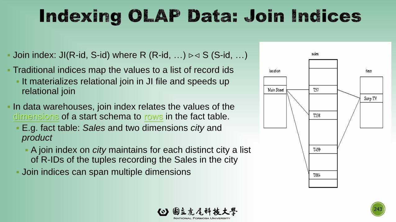
▪ Join index: JI(R-id, S-id) where R (R-id, …) S (S-id, …)
▪ Traditional indices map the values to a list of record ids
▪ It materializes relational join in JI file and speeds up relational join
▪ In data warehouses, join index relates the values of the dimensions of a start schema to rows in the fact table.
▪ E.g. fact table: Sales and two dimensions city and product
▪ A join index on city maintains for each distinct city a list of R-IDs of the tuples recording the Sales in the city
▪ Join indices can span multiple dimensions
243
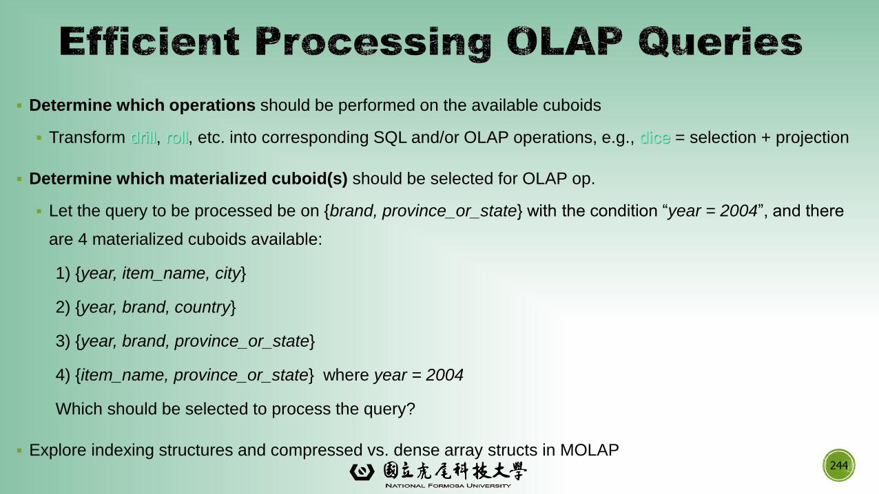
▪ Determine which operations should be performed on the available cuboids
▪ Transform drill, roll, etc. into corresponding SQL and/or OLAP operations, e.g., dice = selection + projection
▪ Determine which materialized cuboid(s) should be selected for OLAP op.
▪ Let the query to be processed be on {brand, province_or_state} with the condition “year = 2004”, and there
are 4 materialized cuboids available:
1) {year, item_name, city}
2) {year, brand, country}
3) {year, brand, province_or_state}
4) {item_name, province_or_state} where year = 2004
Which should be selected to process the query?
▪ Explore indexing structures and compressed vs. dense array structs in MOLAP244
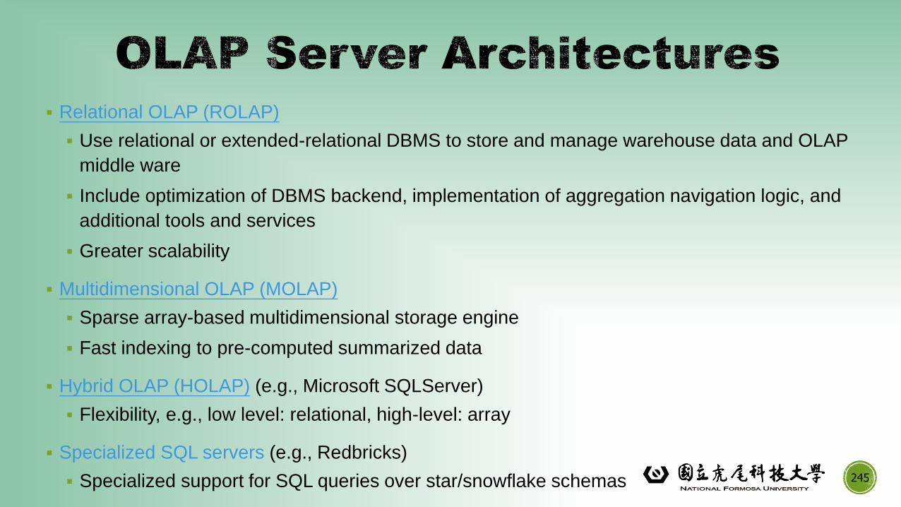
▪ Relational OLAP (ROLAP)
▪ Use relational or extended-relational DBMS to store and manage warehouse data and OLAP
middle ware
▪ Include optimization of DBMS backend, implementation of aggregation navigation logic, and
additional tools and services
▪ Greater scalability
▪ Multidimensional OLAP (MOLAP)
▪ Sparse array-based multidimensional storage engine
▪ Fast indexing to pre-computed summarized data
▪ Hybrid OLAP (HOLAP) (e.g., Microsoft SQLServer)
▪ Flexibility, e.g., low level: relational, high-level: array
▪ Specialized SQL servers (e.g., Redbricks)
▪ Specialized support for SQL queries over star/snowflake schemas 245

Data Warehouse: Basic Concepts
Data Warehouse Modeling: Data Cube and OLAP
Data Warehouse Design and Usage
Data Warehouse Implementation
Data Generalization by Attribute-Oriented Induction
Summary246
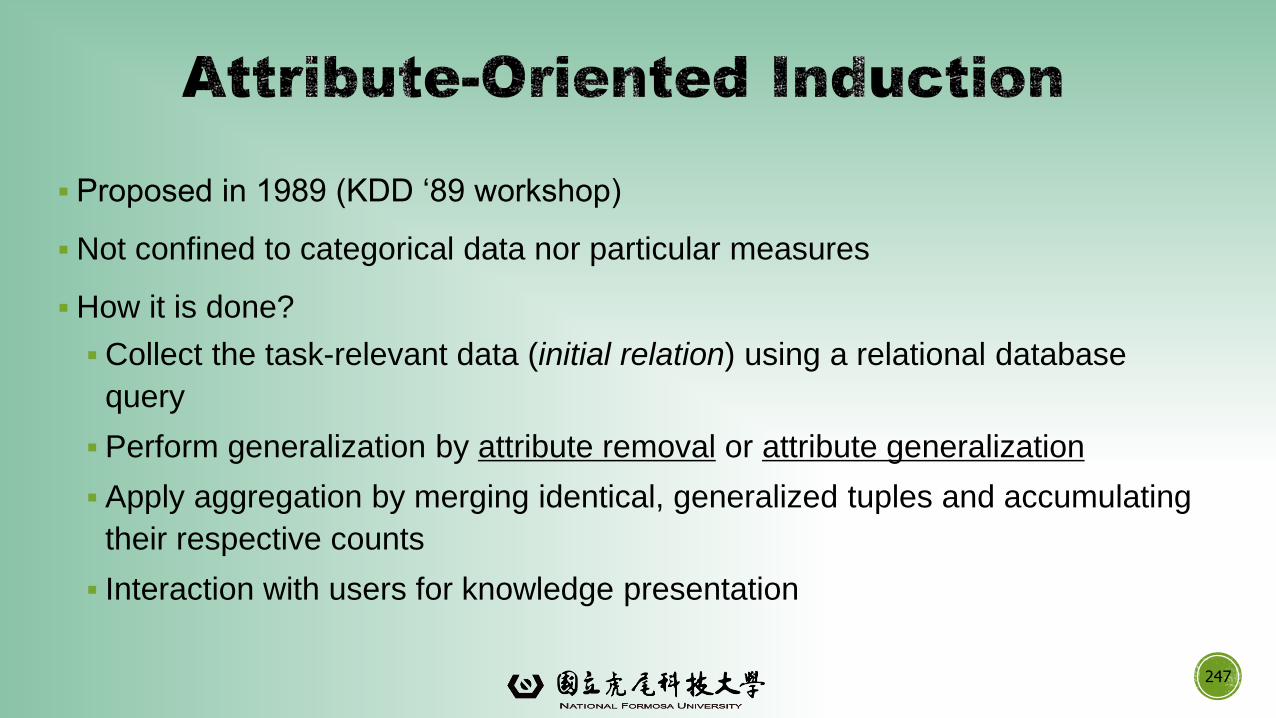
▪ Proposed in 1989 (KDD ‘89 workshop)
▪Not confined to categorical data nor particular measures
▪How it is done?
▪Collect the task-relevant data (initial relation) using a relational database
query
▪ Perform generalization by attribute removal or attribute generalization
▪ Apply aggregation by merging identical, generalized tuples and accumulating
their respective counts
▪ Interaction with users for knowledge presentation
247
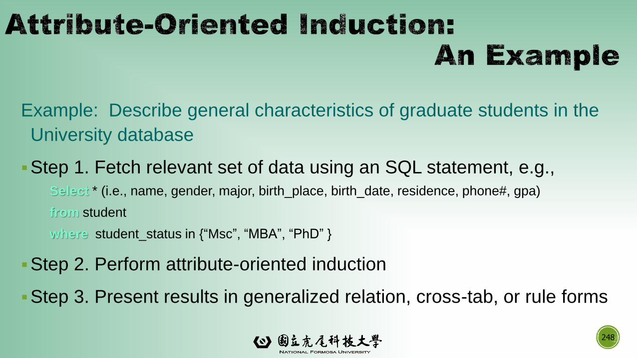
Example: Describe general characteristics of graduate students in the
University database
▪Step 1. Fetch relevant set of data using an SQL statement, e.g.,
Select * (i.e., name, gender, major, birth_place, birth_date, residence, phone#, gpa)
from student
where student_status in {“Msc”, “MBA”, “PhD” }
▪Step 2. Perform attribute-oriented induction
▪Step 3. Present results in generalized relation, cross-tab, or rule forms
248
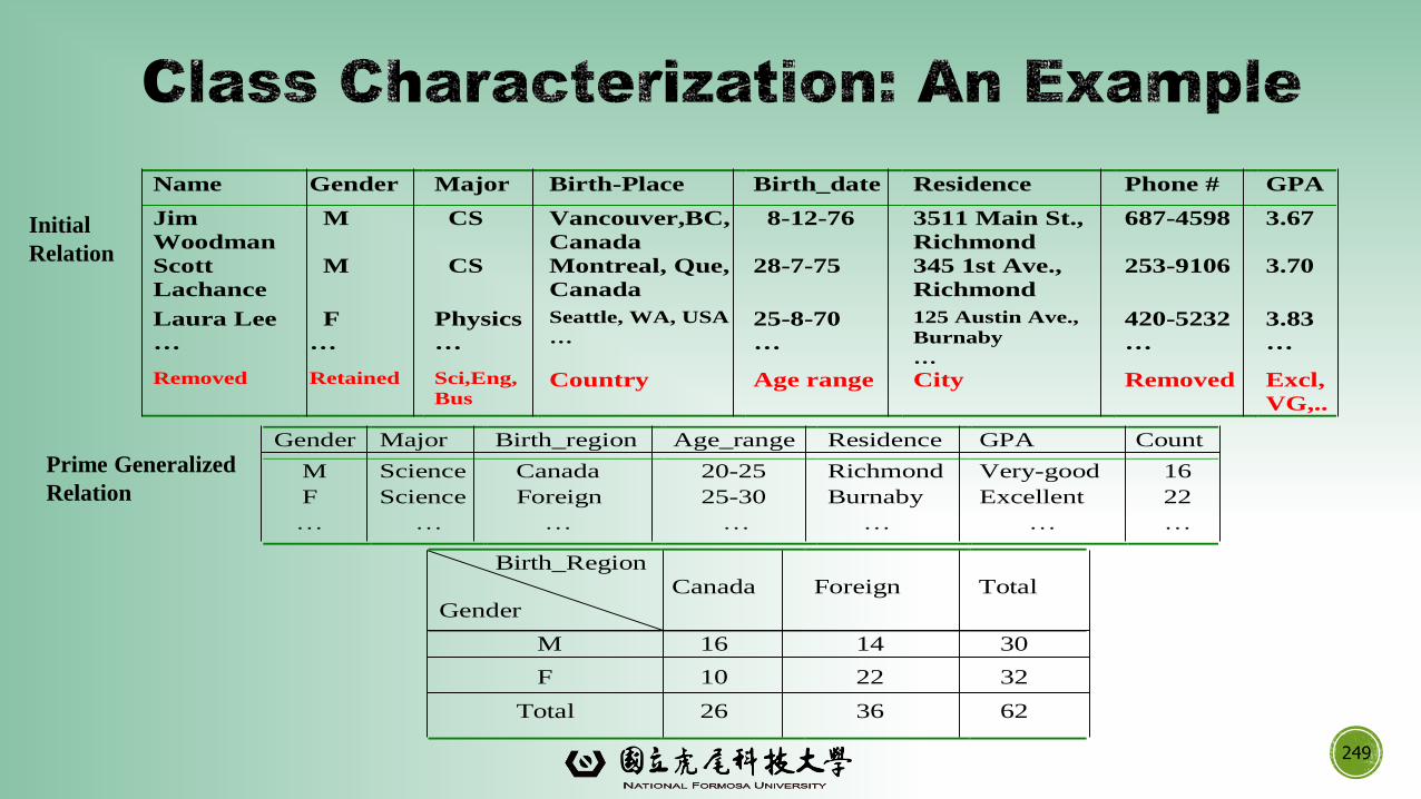
249
Name Gender Major Birth-Place Birth_date Residence Phone # GPA
Jim
Woodman
M CS Vancouver,BC,
Canada
8-12-76 3511 Main St.,
Richmond
687-4598 3.67
Scott
Lachance
M CS Montreal, Que,
Canada
28-7-75 345 1st Ave.,
Richmond
253-9106 3.70
Laura Lee
…
F
…
Physics
…
Seattle, WA, USA
…25-8-70
…
125 Austin Ave.,
Burnaby
…
420-5232
…
3.83
…
Removed Retained Sci,Eng,
BusCountry Age range City Removed Excl,
VG,..
Gender Major Birth_region Age_range Residence GPA Count
M Science Canada 20-25 Richmond Very-good 16
F Science Foreign 25-30 Burnaby Excellent 22
… … … … … … …
Birth_Region
Gender
Canada Foreign Total
M 16 14 30
F 10 22 32
Total 26 36 62
Prime Generalized
Relation
Initial
Relation
▪Data focusing: task-relevant data, including dimensions, and the result is the
initial relation
▪ Attribute-removal: remove attribute A if there is a large set of distinct values for A
but (1) there is no generalization operator on A, or (2) A’s higher level concepts
are expressed in terms of other attributes
▪ Attribute-generalization: If there is a large set of distinct values for A, and there
exists a set of generalization operators on A, then select an operator and
generalize A
▪ Attribute-threshold control: typical 2-8, specified/default
▪Generalized relation threshold control: control the final relation/rule size
250
▪ InitialRel: Query processing of task-relevant data, deriving the initial relation.
▪ PreGen: Based on the analysis of the number of distinct values in each attribute,
determine generalization plan for each attribute: removal? or how high to
generalize?
▪ PrimeGen: Based on the PreGen plan, perform generalization to the right level to
derive a “prime generalized relation”, accumulating the counts.
▪ Presentation: User interaction: (1) adjust levels by drilling, (2) pivoting, (3)
mapping into rules, cross tabs, visualization presentations.
251
▪ Generalized relation:
▪ Relations where some or all attributes are generalized, with counts or other aggregation
values accumulated.
▪ Cross tabulation:
▪ Mapping results into cross tabulation form (similar to contingency tables).
▪ Visualization techniques:
▪ Pie charts, bar charts, curves, cubes, and other visual forms.
▪ Quantitative characteristic rules:
▪ Mapping generalized result into characteristic rules with quantitative information associated
with it, e.g.,
252.%]47:["")(_%]53:["")(_
)()(
tforeignxregionbirthtCanadaxregionbirth
xmalexgrad
▪ Comparison: Comparing two or more classes
▪ Method:
▪ Partition the set of relevant data into the target class and the contrasting class(es)
▪ Generalize both classes to the same high level concepts
▪ Compare tuples with the same high level descriptions
▪ Present for every tuple its description and two measures
▪ support - distribution within single class
▪ comparison - distribution between classes
▪ Highlight the tuples with strong discriminant features
▪ Relevance Analysis:
▪ Find attributes (features) which best distinguish different classes
253
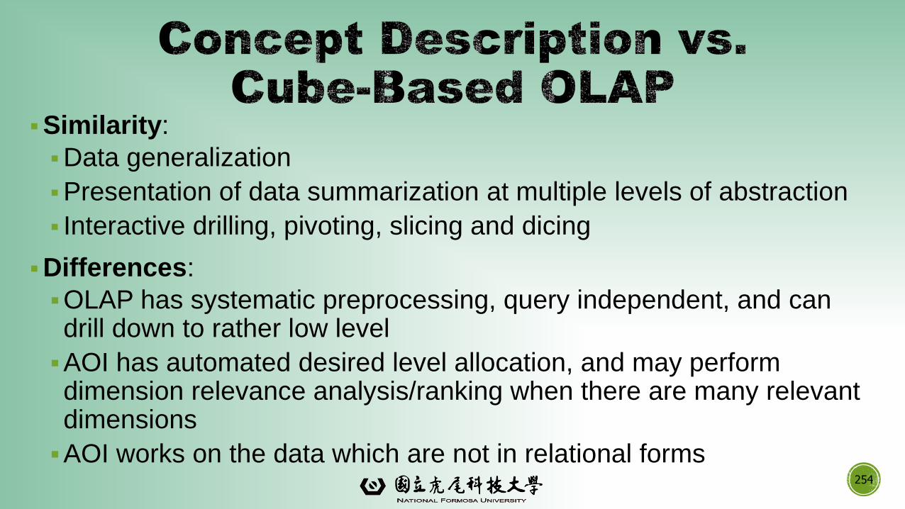
▪Similarity:
▪Data generalization
▪Presentation of data summarization at multiple levels of abstraction
▪ Interactive drilling, pivoting, slicing and dicing
▪Differences:
▪OLAP has systematic preprocessing, query independent, and can drill down to rather low level
▪AOI has automated desired level allocation, and may perform dimension relevance analysis/ranking when there are many relevant dimensions
▪AOI works on the data which are not in relational forms254
Data Warehouse: Basic Concepts
Data Warehouse Modeling: Data Cube and OLAP
Data Warehouse Design and Usage
Data Warehouse Implementation
Data Generalization by Attribute-Oriented Induction
Summary255
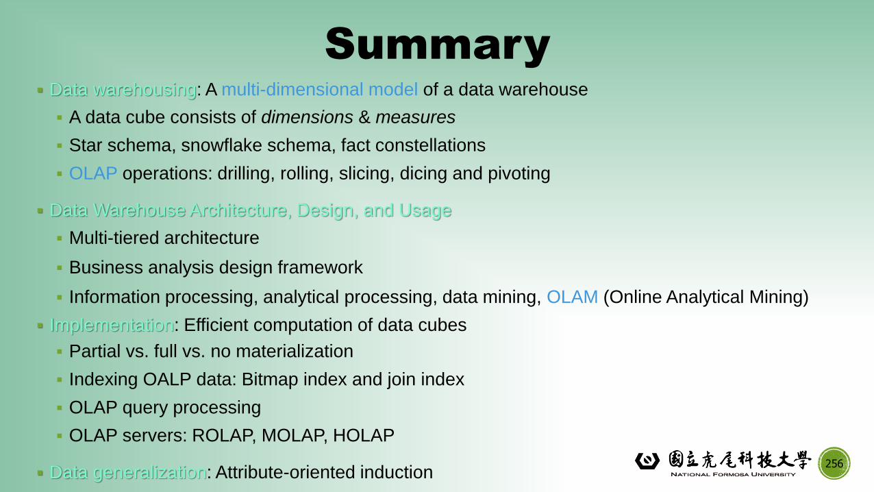
Summary
▪ Data warehousing: A multi-dimensional model of a data warehouse
▪ A data cube consists of dimensions & measures
▪ Star schema, snowflake schema, fact constellations
▪ OLAP operations: drilling, rolling, slicing, dicing and pivoting
▪ Data Warehouse Architecture, Design, and Usage
▪ Multi-tiered architecture
▪ Business analysis design framework
▪ Information processing, analytical processing, data mining, OLAM (Online Analytical Mining)
▪ Implementation: Efficient computation of data cubes
▪ Partial vs. full vs. no materialization
▪ Indexing OALP data: Bitmap index and join index
▪ OLAP query processing
▪ OLAP servers: ROLAP, MOLAP, HOLAP
▪ Data generalization: Attribute-oriented induction256
▪ S. Agarwal, R. Agrawal, P. M. Deshpande, A. Gupta, J. F. Naughton, R. Ramakrishnan, and S. Sarawagi. On the
computation of multidimensional aggregates. VLDB’96
▪ D. Agrawal, A. E. Abbadi, A. Singh, and T. Yurek. Efficient view maintenance in data warehouses. SIGMOD’97
▪ R. Agrawal, A. Gupta, and S. Sarawagi. Modeling multidimensional databases. ICDE’97
▪ S. Chaudhuri and U. Dayal. An overview of data warehousing and OLAP technology. ACM SIGMOD Record,
26:65-74, 1997
▪ E. F. Codd, S. B. Codd, and C. T. Salley. Beyond decision support. Computer World, 27, July 1993.
▪ J. Gray, et al. Data cube: A relational aggregation operator generalizing group-by, cross-tab and sub-totals. Data
Mining and Knowledge Discovery, 1:29-54, 1997.
▪ A. Gupta and I. S. Mumick. Materialized Views: Techniques, Implementations, and Applications. MIT Press, 1999.
▪ J. Han. Towards on-line analytical mining in large databases. ACM SIGMOD Record, 27:97-107, 1998.
▪ V. Harinarayan, A. Rajaraman, and J. D. Ullman. Implementing data cubes efficiently. SIGMOD’96
▪ J. Hellerstein, P. Haas, and H. Wang. Online aggregation. SIGMOD'97
257
▪ C. Imhoff, N. Galemmo, and J. G. Geiger. Mastering Data Warehouse Design: Relational and Dimensional Techniques. John Wiley, 2003
▪ W. H. Inmon. Building the Data Warehouse. John Wiley, 1996
▪ R. Kimball and M. Ross. The Data Warehouse Toolkit: The Complete Guide to Dimensional Modeling. 2ed. John Wiley, 2002
▪ P. O’Neil and G. Graefe. Multi-table joins through bitmapped join indices. SIGMOD Record, 24:8–11, Sept. 1995.
▪ P. O'Neil and D. Quass. Improved query performance with variant indexes. SIGMOD'97
▪ Microsoft. OLEDB for OLAP programmer's reference version 1.0. In http://www.microsoft.com/data/oledb/olap, 1998
▪ S. Sarawagi and M. Stonebraker. Efficient organization of large multidimensional arrays. ICDE'94
▪ A. Shoshani. OLAP and statistical databases: Similarities and differences. PODS’00.
▪ D. Srivastava, S. Dar, H. V. Jagadish, and A. V. Levy. Answering queries with aggregation using views. VLDB'96
▪ P. Valduriez. Join indices. ACM Trans. Database Systems, 12:218-246, 1987.
▪ J. Widom. Research problems in data warehousing. CIKM’95
▪ K. Wu, E. Otoo, and A. Shoshani, Optimal Bitmap Indices with Efficient Compression, ACM Trans. on Database Systems (TODS), 31(1): 1-38, 2006 258
259
Data Cube Computation: Preliminary Concepts
Data Cube Computation Methods
Processing Advanced Queries by Exploring Data Cube
Technology
Multidimensional Data Analysis in Cube Space
Summary
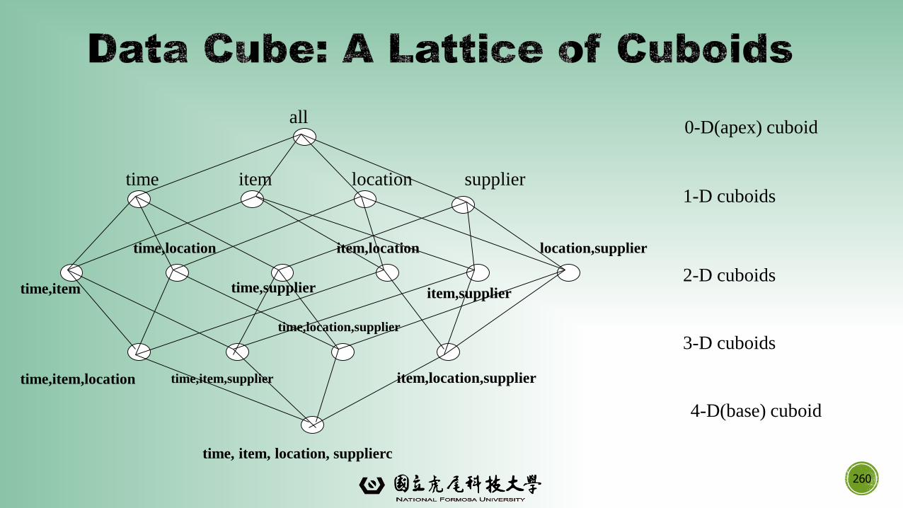
260
time,item
time,item,location
time, item, location, supplierc
all
time item location supplier
time,location
time,supplier
item,location
item,supplier
location,supplier
time,item,supplier
time,location,supplier
item,location,supplier
0-D(apex) cuboid
1-D cuboids
2-D cuboids
3-D cuboids
4-D(base) cuboid

▪ Base vs. aggregate cells; ancestor vs. descendant cells; parent vs. child cells1. (9/15, milk, Urbana, Dairy_land)
2. (9/15, milk, Urbana, *)
3. (*, milk, Urbana, *)
4. (*, milk, Urbana, *)
5. (*, milk, Chicago, *)
6. (*, milk, *, *) 261
all
time,item
time,item,location
time, item, location, supplier
time item location supplier
time,location
time,supplier
item,location
item,supplier
location,supplier
time,item,supplier
time,location,supplier
item,location,supplier
0-D(apex) cuboid
1-D cuboids
2-D cuboids
3-D cuboids
4-D(base) cuboid
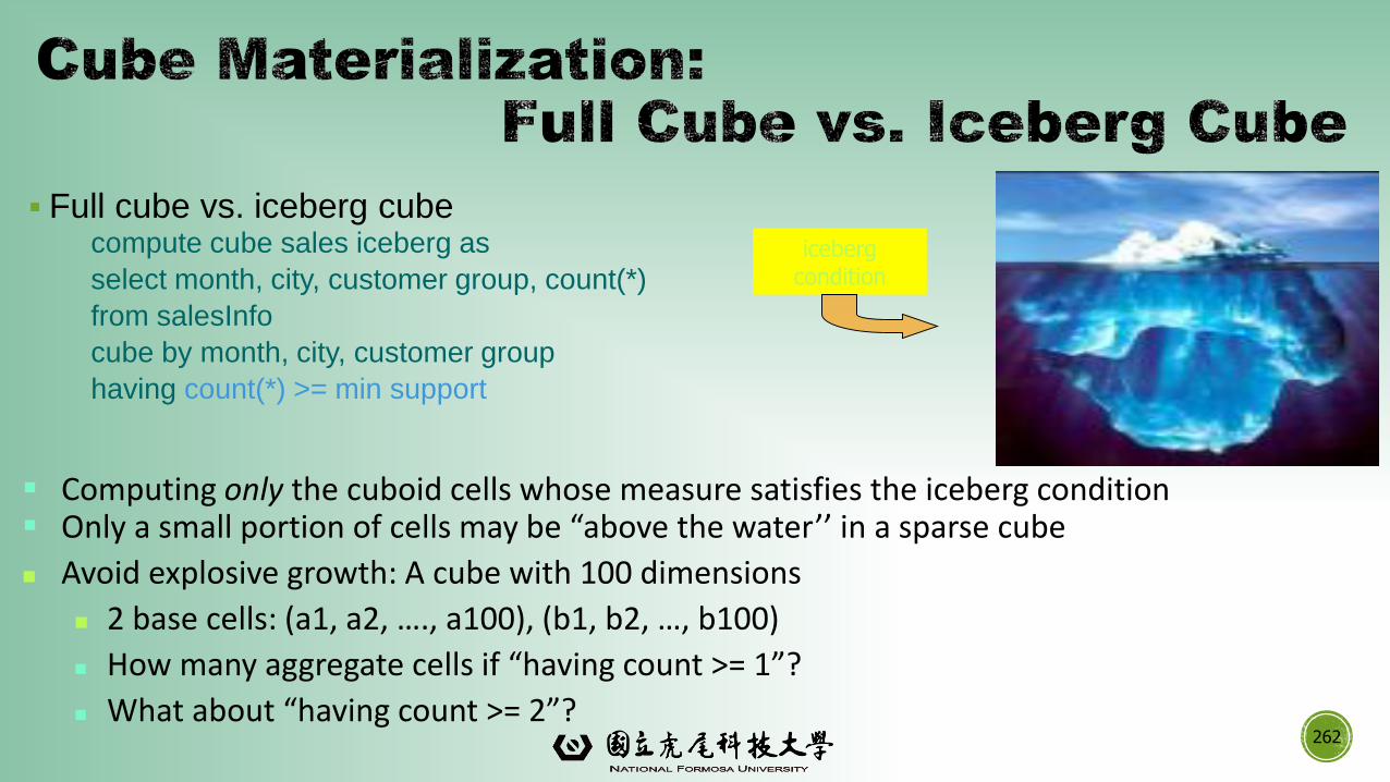
262
▪ Full cube vs. iceberg cubecompute cube sales iceberg as
select month, city, customer group, count(*)
from salesInfo
cube by month, city, customer group
having count(*) >= min support
▪ Computing only the cuboid cells whose measure satisfies the iceberg condition ▪ Only a small portion of cells may be “above the water’’ in a sparse cube
Avoid explosive growth: A cube with 100 dimensions
2 base cells: (a1, a2, …., a100), (b1, b2, …, b100)
How many aggregate cells if “having count >= 1”?
What about “having count >= 2”?
iceberg condition
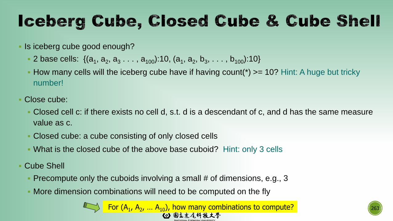
▪ Is iceberg cube good enough?
▪ 2 base cells: {(a1, a2, a3 . . . , a100):10, (a1, a2, b3, . . . , b100):10}
▪ How many cells will the iceberg cube have if having count(*) >= 10? Hint: A huge but tricky
number!
▪ Close cube:
▪ Closed cell c: if there exists no cell d, s.t. d is a descendant of c, and d has the same measure
value as c.
▪ Closed cube: a cube consisting of only closed cells
▪ What is the closed cube of the above base cuboid? Hint: only 3 cells
▪ Cube Shell
▪ Precompute only the cuboids involving a small # of dimensions, e.g., 3
▪ More dimension combinations will need to be computed on the fly
263For (A1, A2, … A10), how many combinations to compute?
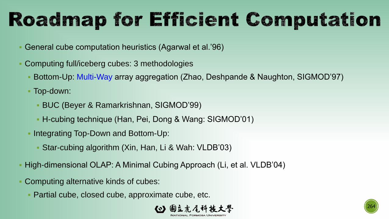
▪ General cube computation heuristics (Agarwal et al.’96)
▪ Computing full/iceberg cubes: 3 methodologies
▪ Bottom-Up: Multi-Way array aggregation (Zhao, Deshpande & Naughton, SIGMOD’97)
▪ Top-down:
▪ BUC (Beyer & Ramarkrishnan, SIGMOD’99)
▪ H-cubing technique (Han, Pei, Dong & Wang: SIGMOD’01)
▪ Integrating Top-Down and Bottom-Up:
▪ Star-cubing algorithm (Xin, Han, Li & Wah: VLDB’03)
▪ High-dimensional OLAP: A Minimal Cubing Approach (Li, et al. VLDB’04)
▪ Computing alternative kinds of cubes:
▪ Partial cube, closed cube, approximate cube, etc.
264
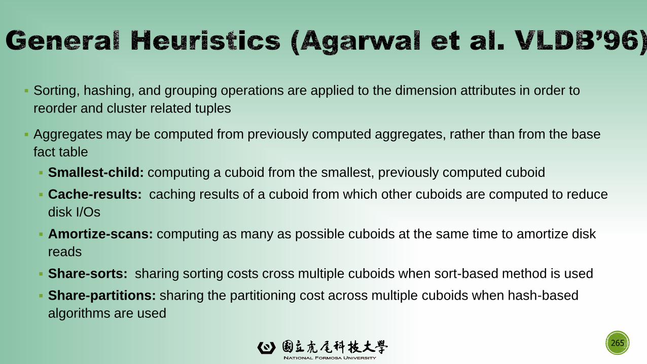
▪ Sorting, hashing, and grouping operations are applied to the dimension attributes in order to
reorder and cluster related tuples
▪ Aggregates may be computed from previously computed aggregates, rather than from the base
fact table
▪ Smallest-child: computing a cuboid from the smallest, previously computed cuboid
▪ Cache-results: caching results of a cuboid from which other cuboids are computed to reduce
disk I/Os
▪ Amortize-scans: computing as many as possible cuboids at the same time to amortize disk
reads
▪ Share-sorts: sharing sorting costs cross multiple cuboids when sort-based method is used
▪ Share-partitions: sharing the partitioning cost across multiple cuboids when hash-based
algorithms are used
265
266
▪Data Cube Computation: Preliminary Concepts
▪Data Cube Computation Methods
▪ Processing Advanced Queries by Exploring Data Cube Technology
▪Multidimensional Data Analysis in Cube Space
▪ Summary
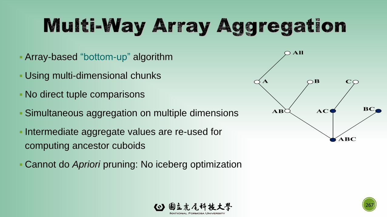
▪ Array-based “bottom-up” algorithm
▪Using multi-dimensional chunks
▪No direct tuple comparisons
▪ Simultaneous aggregation on multiple dimensions
▪ Intermediate aggregate values are re-used for
computing ancestor cuboids
▪Cannot do Apriori pruning: No iceberg optimization
267
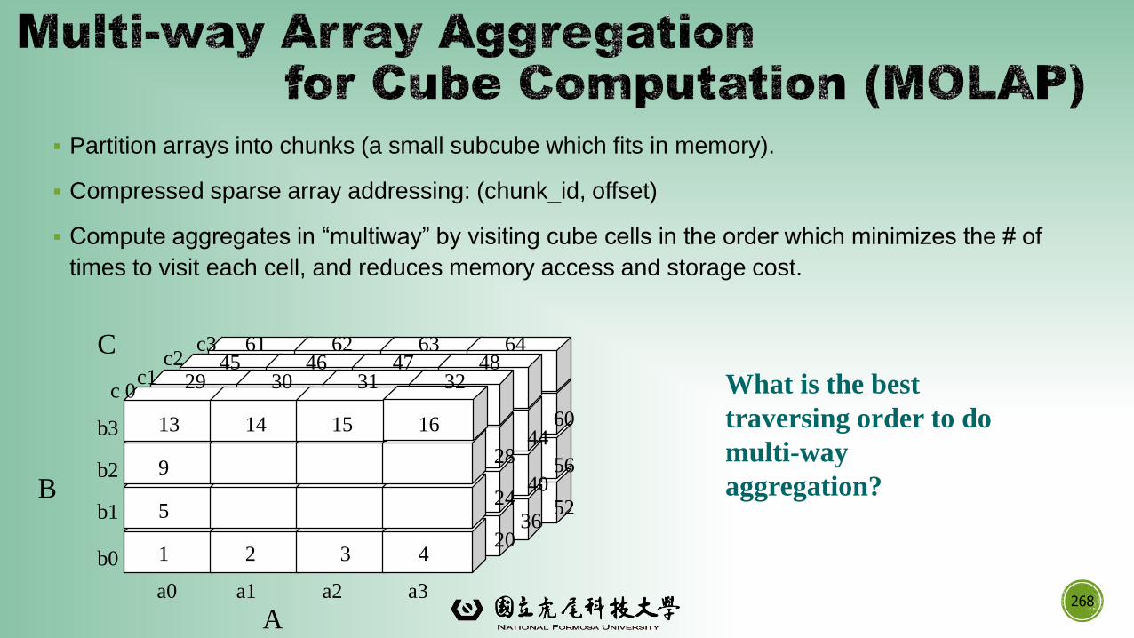
▪ Partition arrays into chunks (a small subcube which fits in memory).
▪ Compressed sparse array addressing: (chunk_id, offset)
▪ Compute aggregates in “multiway” by visiting cube cells in the order which minimizes the # of
times to visit each cell, and reduces memory access and storage cost.
268
What is the best
traversing order to do
multi-way
aggregation?
A
B
29 30 31 32
1 2 3 4
5
9
13 14 15 16
6463626148474645
a1a0
c3c2
c1c 0
b3
b2
b1
b0
a2 a3
C
B
4428 56
4024 52
3620
60
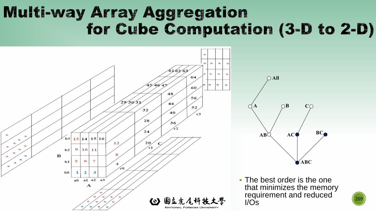
all
A B
AB
ABC
AC BC
C
269
▪ The best order is the one that minimizes the memory requirement and reduced I/Os
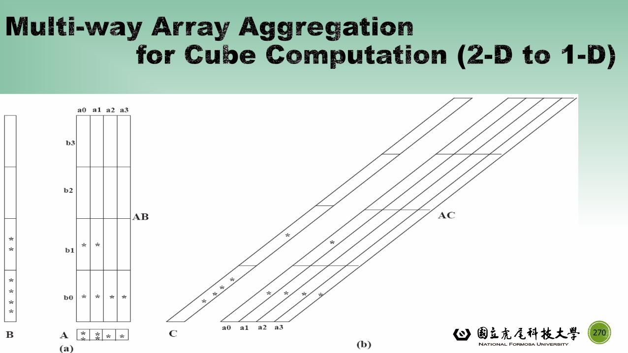
270
▪Method: the planes should be sorted and computed according to their
size in ascending order
▪ Idea: keep the smallest plane in the main memory, fetch and compute
only one chunk at a time for the largest plane
▪Limitation of the method: computing well only for a small number of
dimensions
▪ If there are a large number of dimensions, “top-down” computation and
iceberg cube computation methods can be explored
271
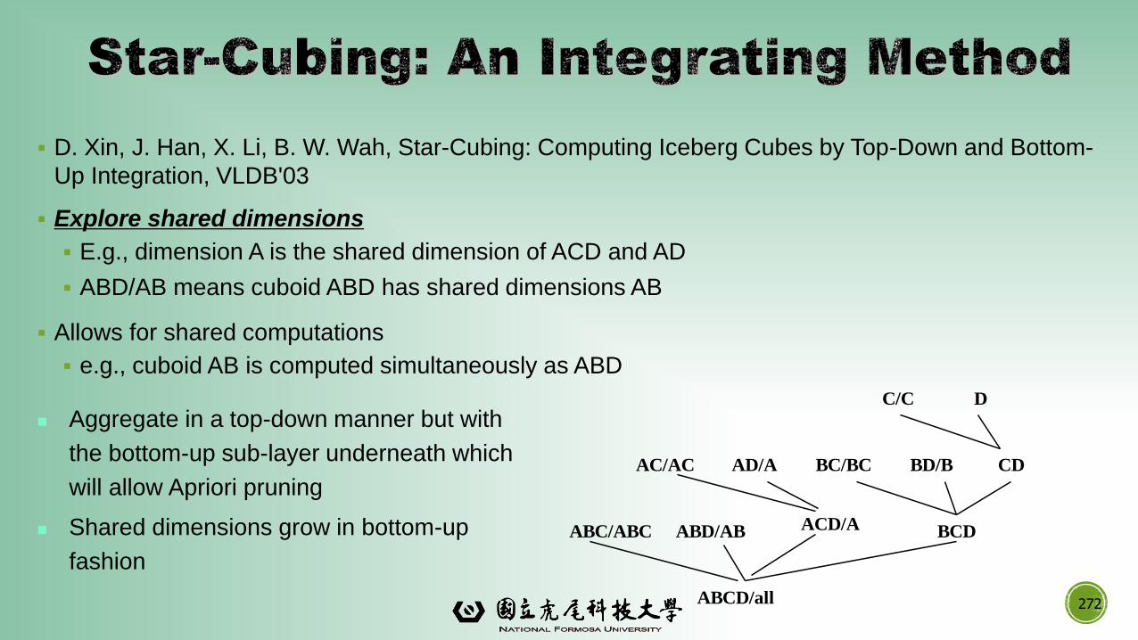
▪ D. Xin, J. Han, X. Li, B. W. Wah, Star-Cubing: Computing Iceberg Cubes by Top-Down and Bottom-
Up Integration, VLDB'03
▪ Explore shared dimensions
▪ E.g., dimension A is the shared dimension of ACD and AD
▪ ABD/AB means cuboid ABD has shared dimensions AB
▪ Allows for shared computations
▪ e.g., cuboid AB is computed simultaneously as ABD
C/C
AC/AC BC/BC
ABC/ABC ABD/AB ACD/A BCD
AD/A BD/B CD
D
ABCD/all 272
Aggregate in a top-down manner but with
the bottom-up sub-layer underneath which
will allow Apriori pruning
Shared dimensions grow in bottom-up
fashion
▪Anti-monotonic property of shared dimensions
▪ If the measure is anti-monotonic, and if the aggregate value
on a shared dimension does not satisfy the iceberg condition,
then all the cells extended from this shared dimension cannot
satisfy the condition either
▪ Intuition: if we can compute the shared dimensions before the
actual cuboid, we can use them to do Apriori pruning
▪Problem: how to prune while still aggregate simultaneously on
multiple dimensions?
273
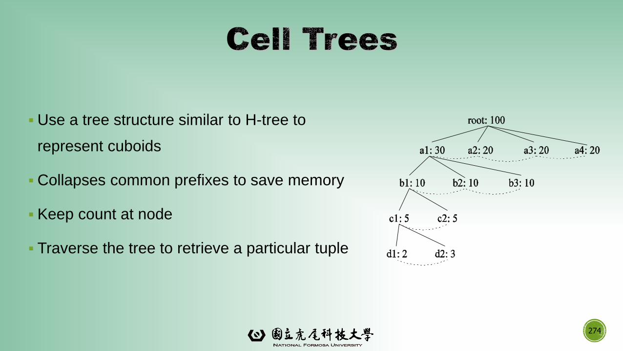
274
▪Use a tree structure similar to H-tree to
represent cuboids
▪Collapses common prefixes to save memory
▪ Keep count at node
▪ Traverse the tree to retrieve a particular tuple
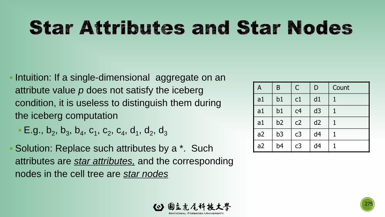
▪ Intuition: If a single-dimensional aggregate on an
attribute value p does not satisfy the iceberg
condition, it is useless to distinguish them during
the iceberg computation
▪ E.g., b2, b3, b4, c1, c2, c4, d1, d2, d3
▪ Solution: Replace such attributes by a *. Such
attributes are star attributes, and the corresponding
nodes in the cell tree are star nodes
A B C D Count
a1 b1 c1 d1 1
a1 b1 c4 d3 1
a1 b2 c2 d2 1
a2 b3 c3 d4 1
a2 b4 c3 d4 1
275
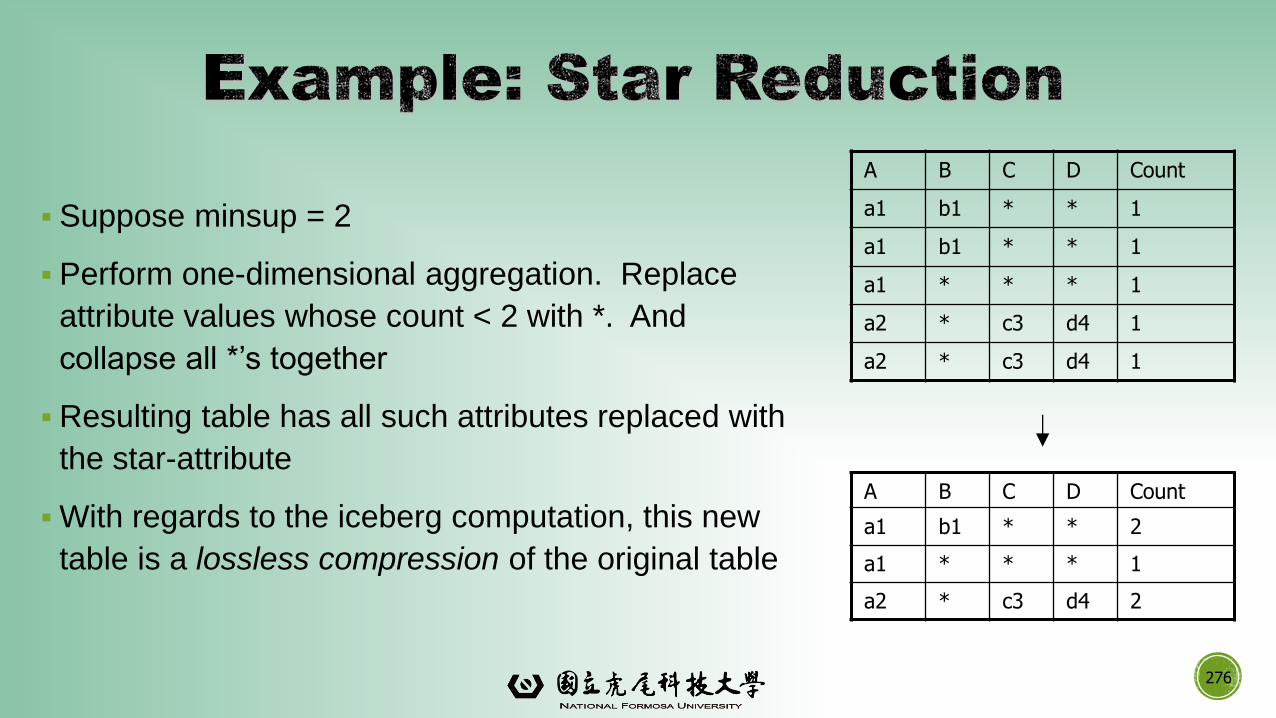
▪ Suppose minsup = 2
▪ Perform one-dimensional aggregation. Replace
attribute values whose count < 2 with *. And
collapse all *’s together
▪Resulting table has all such attributes replaced with
the star-attribute
▪With regards to the iceberg computation, this new
table is a lossless compression of the original table
A B C D Count
a1 b1 * * 1
a1 b1 * * 1
a1 * * * 1
a2 * c3 d4 1
a2 * c3 d4 1
276
A B C D Count
a1 b1 * * 2
a1 * * * 1
a2 * c3 d4 2
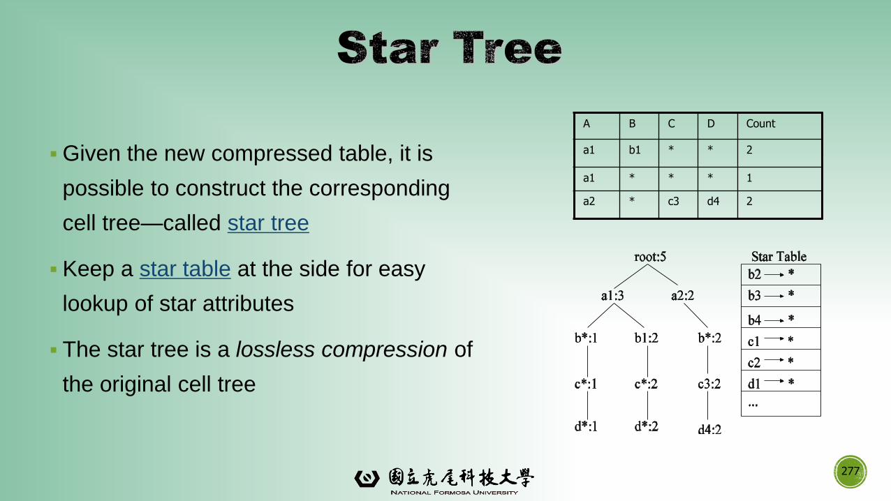
▪Given the new compressed table, it is
possible to construct the corresponding
cell tree—called star tree
▪ Keep a star table at the side for easy
lookup of star attributes
▪ The star tree is a lossless compression of
the original cell tree
A B C D Count
a1 b1 * * 2
a1 * * * 1
a2 * c3 d4 2
277
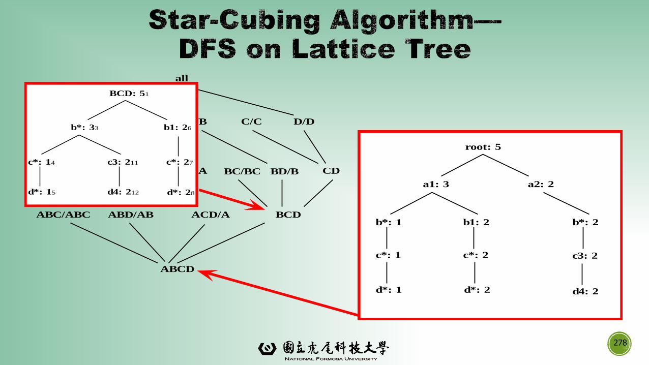
278
all
A B/B C/C
AC/AC BC/BC
ABC/ABC ABD/AB ACD/A BCD
AD/A BD/B CD
D/D
ABCD
/A
AB/AB
BCD: 51
b*: 33 b1: 26
c*: 27c3: 211c*: 14
d*: 15 d4: 212 d*: 28
root: 5
a1: 3 a2: 2
b*: 2b1: 2b*: 1
d*: 1
c*: 1
d*: 2
c*: 2
d4: 2
c3: 2
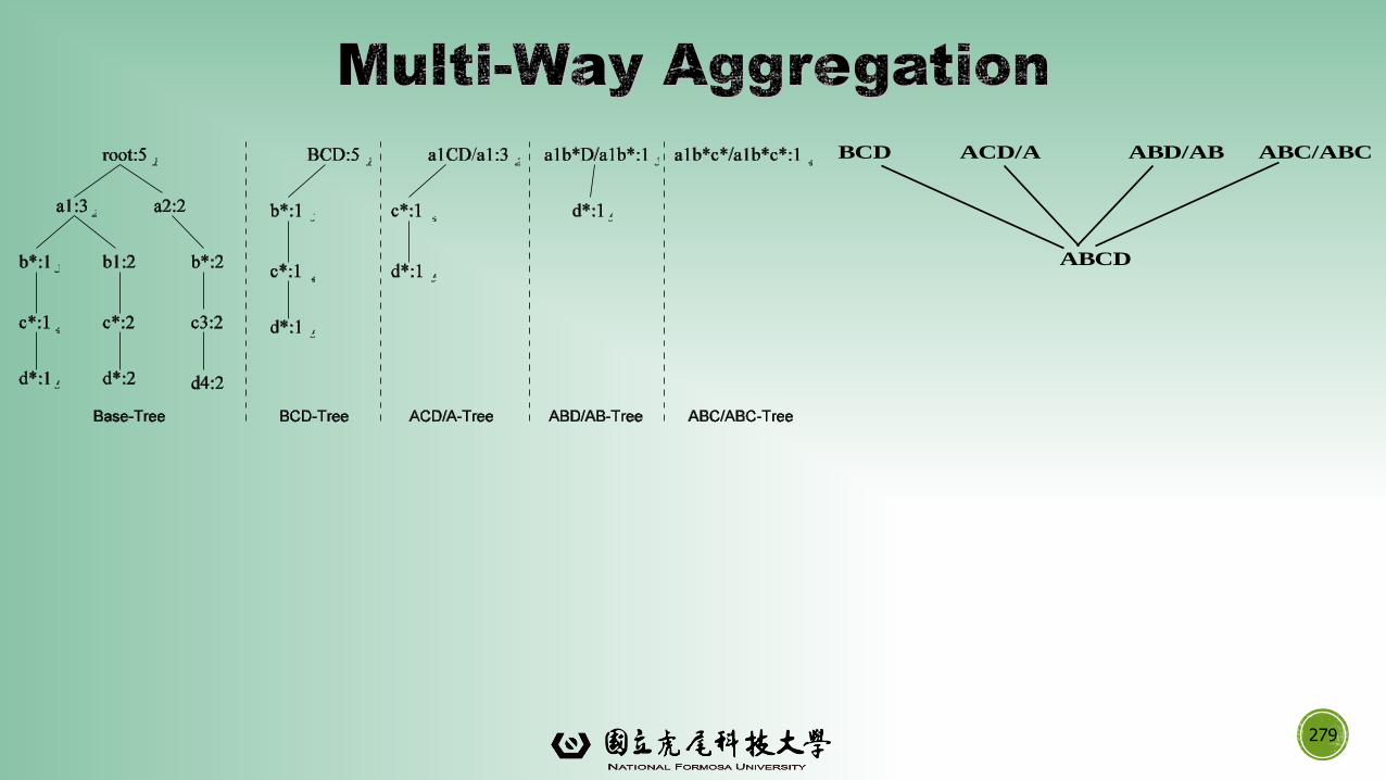
279
ABC/ABCABD/ABACD/ABCD
ABCD
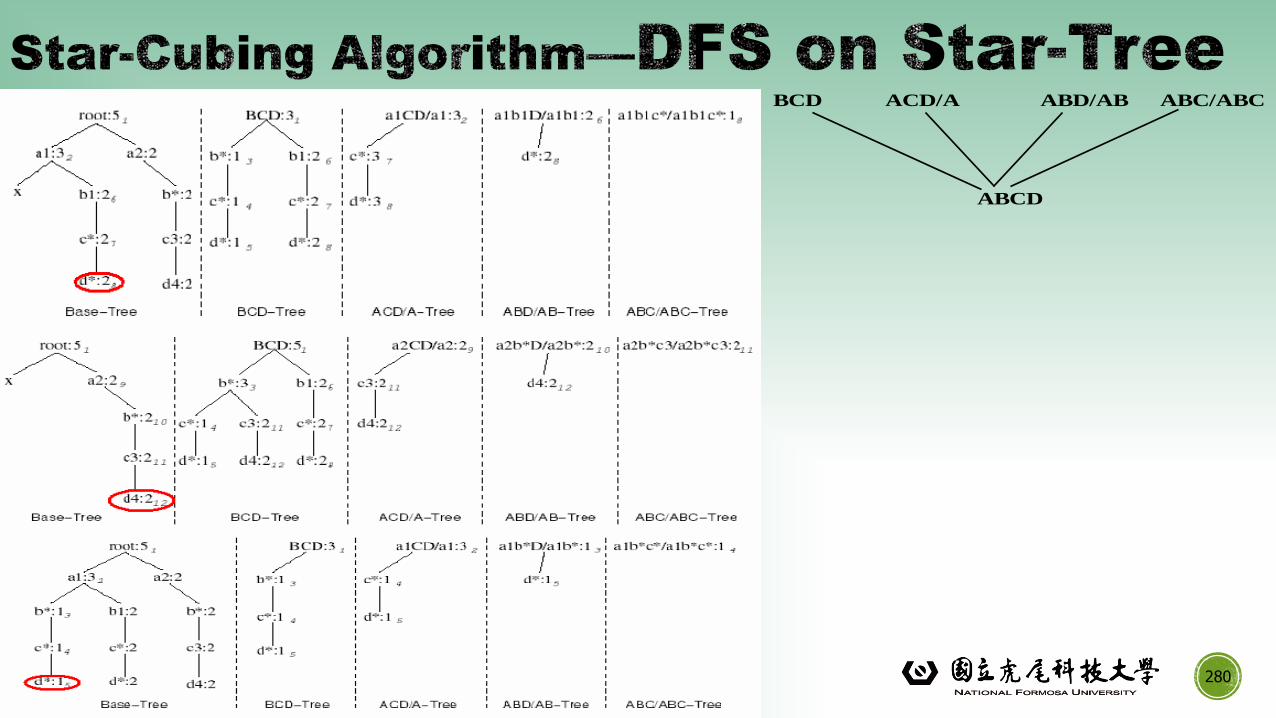
280
ABC/ABCABD/ABACD/ABCD
ABCD
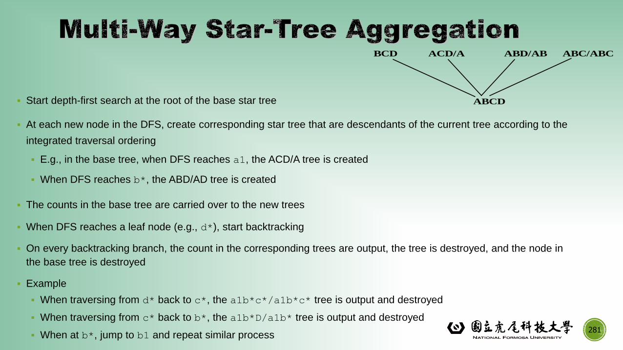
▪ Start depth-first search at the root of the base star tree
▪ At each new node in the DFS, create corresponding star tree that are descendants of the current tree according to the
integrated traversal ordering
▪ E.g., in the base tree, when DFS reaches a1, the ACD/A tree is created
▪ When DFS reaches b*, the ABD/AD tree is created
▪ The counts in the base tree are carried over to the new trees
▪ When DFS reaches a leaf node (e.g., d*), start backtracking
▪ On every backtracking branch, the count in the corresponding trees are output, the tree is destroyed, and the node in
the base tree is destroyed
▪ Example
▪ When traversing from d* back to c*, the a1b*c*/a1b*c* tree is output and destroyed
▪ When traversing from c* back to b*, the a1b*D/a1b* tree is output and destroyed
▪ When at b*, jump to b1 and repeat similar process281
ABC/ABCABD/ABACD/ABCD
ABCD
282
Multi-Way Array Aggregation
BUC
Star-Cubing
High-Dimensional OLAP
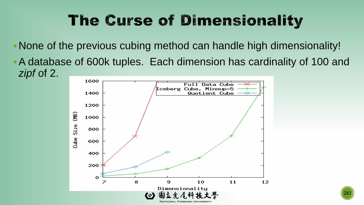
▪None of the previous cubing method can handle high dimensionality!
▪A database of 600k tuples. Each dimension has cardinality of 100 and zipf of 2.
283
▪ X. Li, J. Han, and H. Gonzalez, High-Dimensional OLAP: A Minimal Cubing Approach, VLDB'04
▪Challenge to current cubing methods:
▪ The “curse of dimensionality’’ problem
▪ Iceberg cube and compressed cubes: only delay the inevitable explosion
▪ Full materialization: still significant overhead in accessing results on disk
▪High-D OLAP is needed in applications
▪ Science and engineering analysis
▪ Bio-data analysis: thousands of genes
▪ Statistical surveys: hundreds of variables
284
▪Observation: OLAP occurs only on a small subset of dimensions at a time
▪ Semi-Online Computational Model
1.Partition the set of dimensions into shell fragments
2.Compute data cubes for each shell fragment while retaining inverted
indices or value-list indices
3.Given the pre-computed fragment cubes, dynamically compute cube cells
of the high-dimensional data cube online
285
▪ Partitions the data vertically
▪ Reduces high-dimensional cube into a set of lower dimensional cubes
▪ Online re-construction of original high-dimensional space
▪ Lossless reduction
▪ Offers tradeoffs between the amount of pre-processing and the speed of
online computation
286
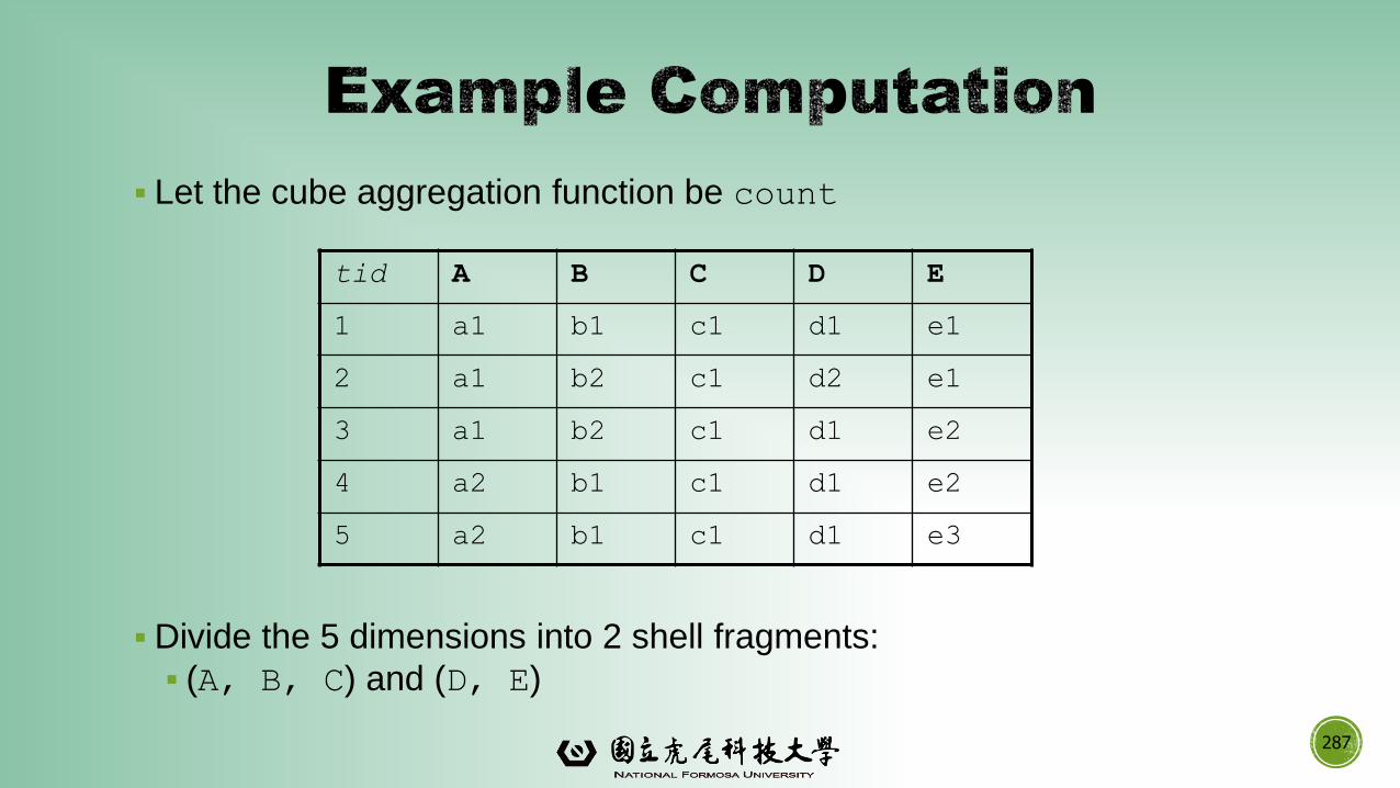
▪ Let the cube aggregation function be count
▪Divide the 5 dimensions into 2 shell fragments:
▪ (A, B, C) and (D, E)
287
tid A B C D E
1 a1 b1 c1 d1 e1
2 a1 b2 c1 d2 e1
3 a1 b2 c1 d1 e2
4 a2 b1 c1 d1 e2
5 a2 b1 c1 d1 e3
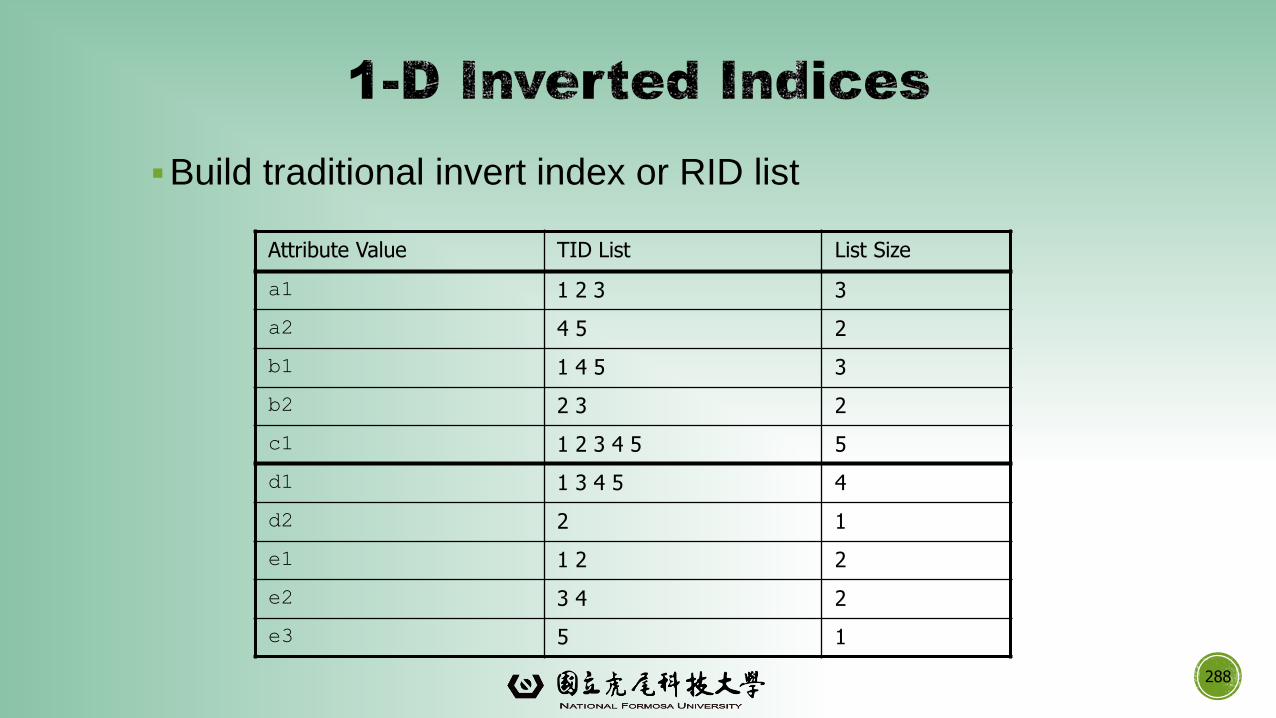
▪Build traditional invert index or RID list
288
Attribute Value TID List List Size
a1 1 2 3 3
a2 4 5 2
b1 1 4 5 3
b2 2 3 2
c1 1 2 3 4 5 5
d1 1 3 4 5 4
d2 2 1
e1 1 2 2
e2 3 4 2
e3 5 1
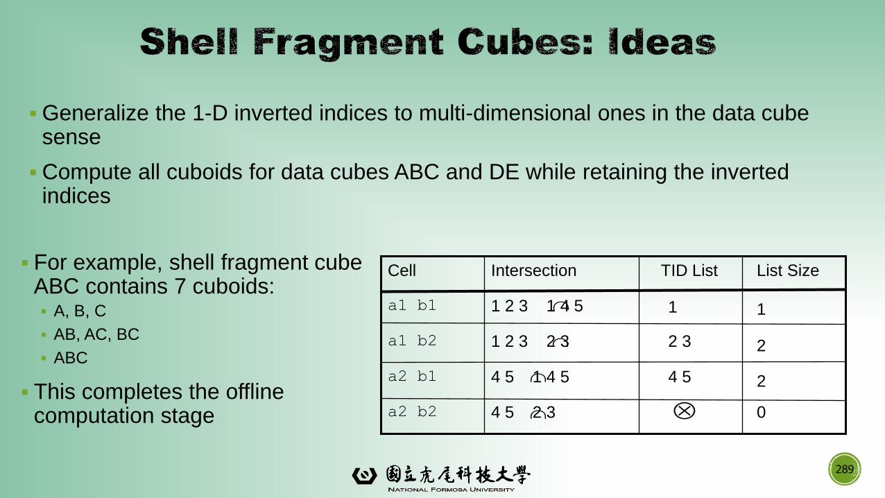
▪Generalize the 1-D inverted indices to multi-dimensional ones in the data cube sense
▪Compute all cuboids for data cubes ABC and DE while retaining the inverted indices
▪ For example, shell fragment cube ABC contains 7 cuboids:▪ A, B, C
▪ AB, AC, BC
▪ ABC
▪ This completes the offline computation stage
289
111 2 3 1 4 5a1 b1
04 5 2 3a2 b2
24 54 5 1 4 5a2 b1
22 31 2 3 2 3a1 b2
List SizeTID ListIntersectionCell
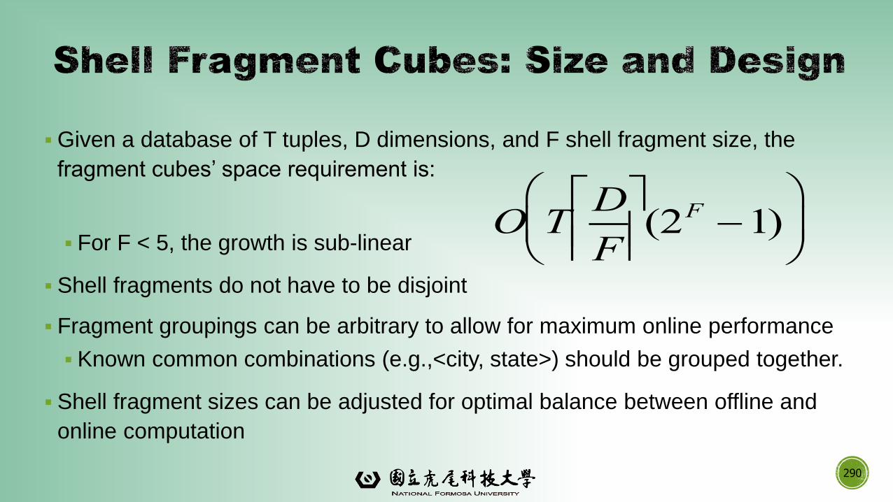
▪Given a database of T tuples, D dimensions, and F shell fragment size, the
fragment cubes’ space requirement is:
▪ For F < 5, the growth is sub-linear
▪ Shell fragments do not have to be disjoint
▪ Fragment groupings can be arbitrary to allow for maximum online performance
▪ Known common combinations (e.g.,<city, state>) should be grouped together.
▪ Shell fragment sizes can be adjusted for optimal balance between offline and
online computation
290
O TD
F
(2F 1)
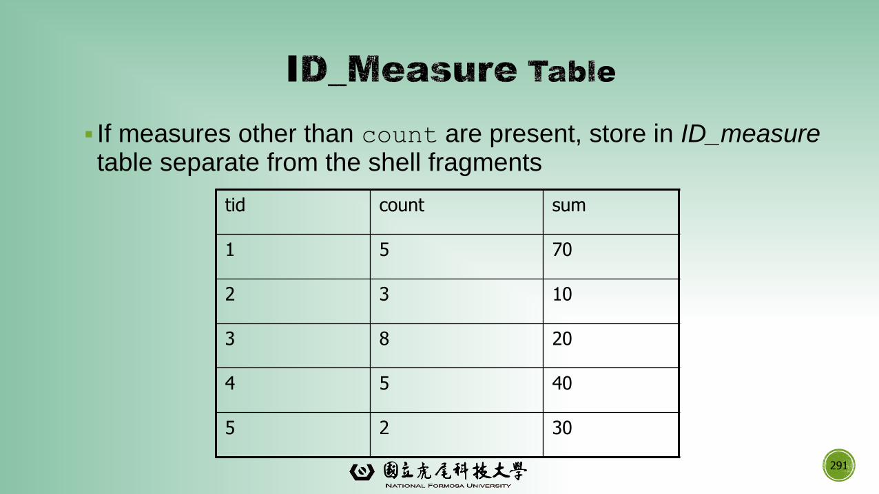
▪ If measures other than count are present, store in ID_measuretable separate from the shell fragments
291
tid count sum
1 5 70
2 3 10
3 8 20
4 5 40
5 2 30
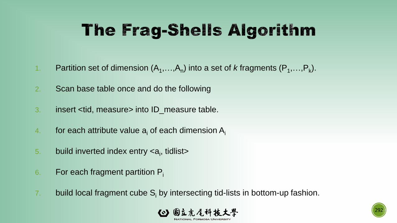
1. Partition set of dimension (A1,…,An) into a set of k fragments (P1,…,Pk).
2. Scan base table once and do the following
3. insert <tid, measure> into ID_measure table.
4. for each attribute value ai of each dimension Ai
5. build inverted index entry <ai, tidlist>
6. For each fragment partition Pi
7. build local fragment cube Si by intersecting tid-lists in bottom-up fashion.
292
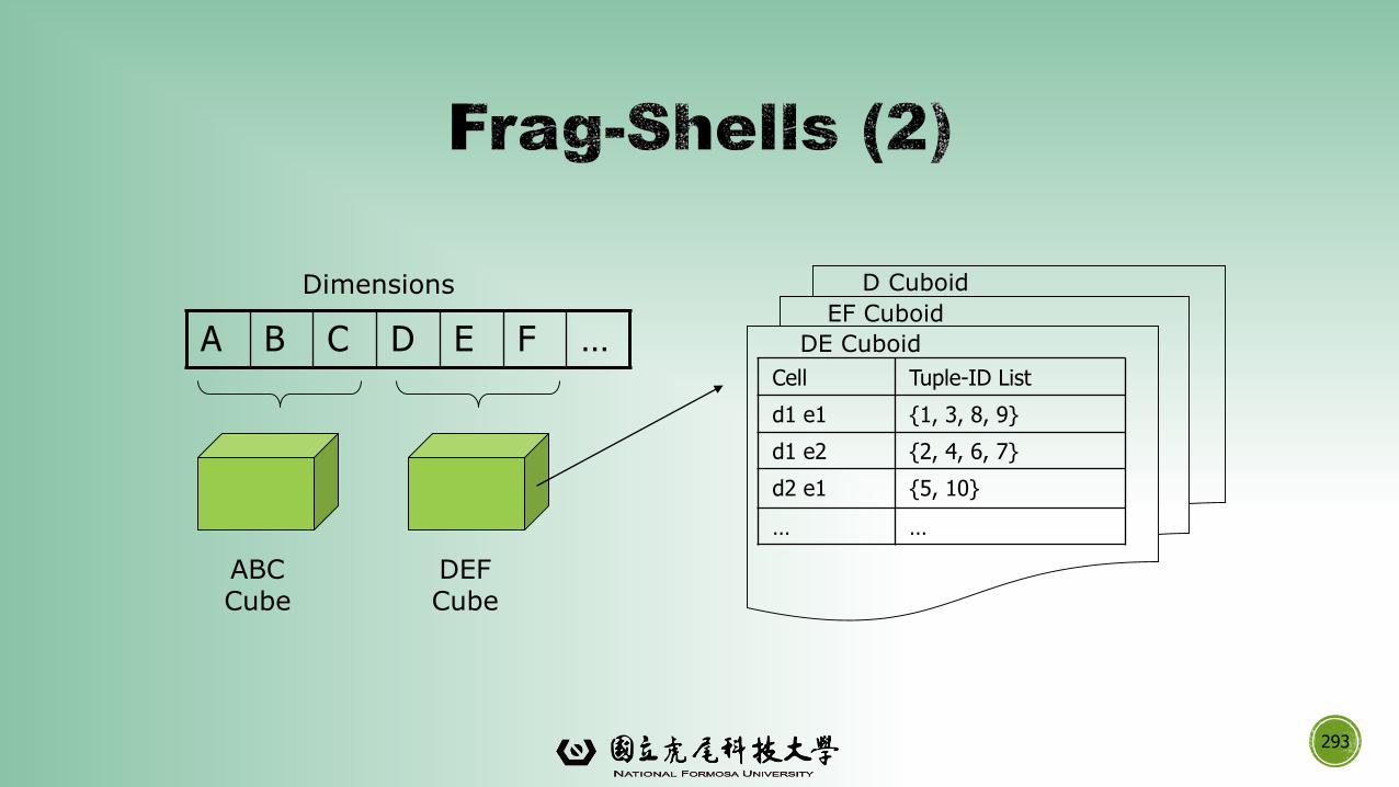
293
A B C D E F …
ABCCube
DEFCube
D Cuboid
EF Cuboid
DE Cuboid
Cell Tuple-ID List
d1 e1 {1, 3, 8, 9}
d1 e2 {2, 4, 6, 7}
d2 e1 {5, 10}
… …
Dimensions
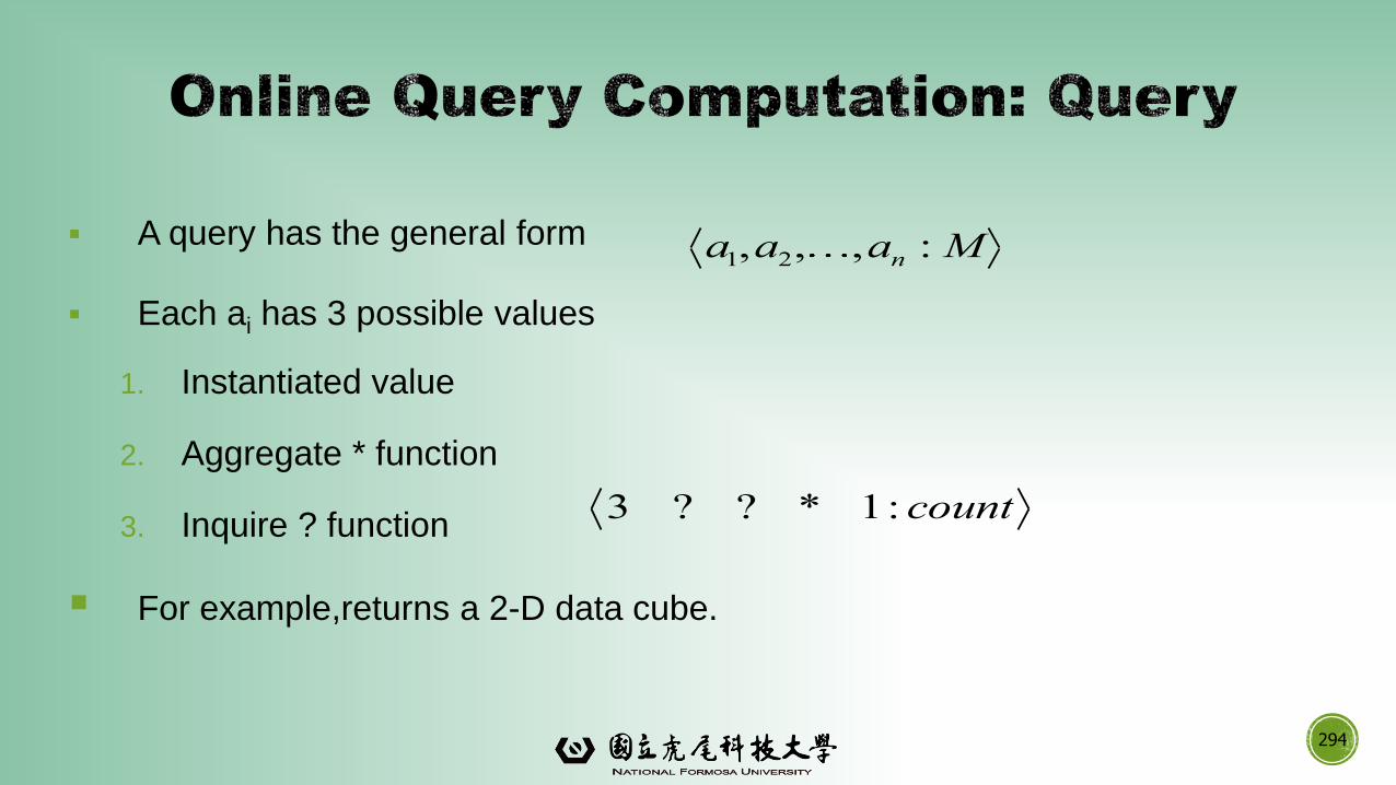
▪ A query has the general form
▪ Each ai has 3 possible values
1. Instantiated value
2. Aggregate * function
3. Inquire ? function
▪ For example,returns a 2-D data cube.
294
a1,a2, ,an :M
3 ? ? * 1: count
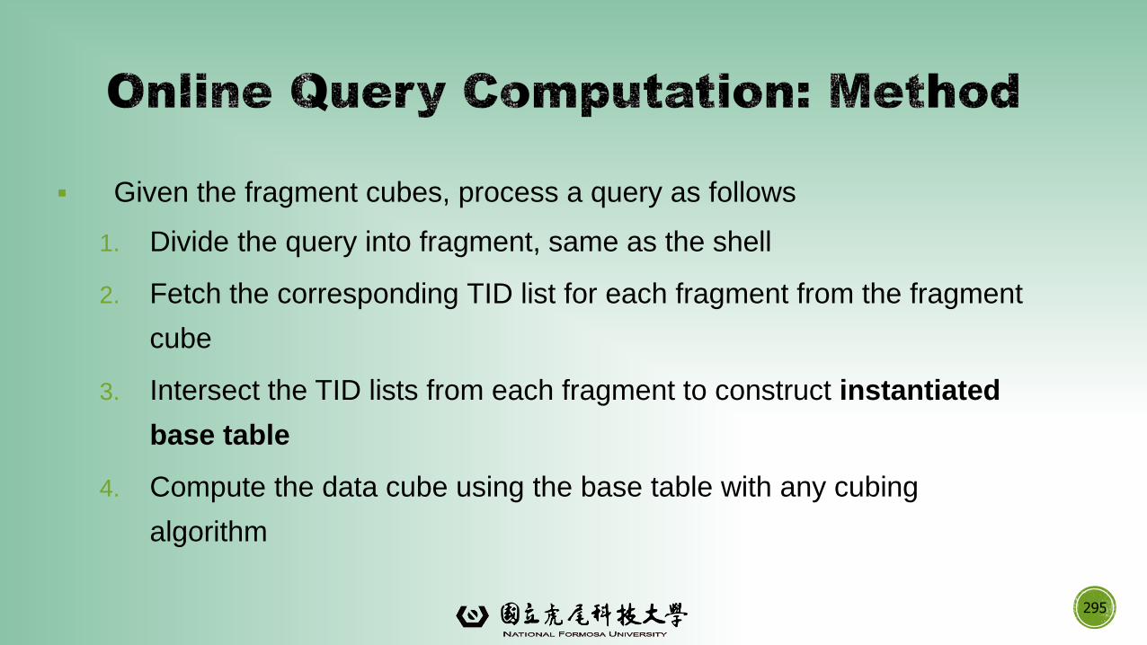
▪ Given the fragment cubes, process a query as follows
1. Divide the query into fragment, same as the shell
2. Fetch the corresponding TID list for each fragment from the fragment
cube
3. Intersect the TID lists from each fragment to construct instantiated
base table
4. Compute the data cube using the base table with any cubing
algorithm
295
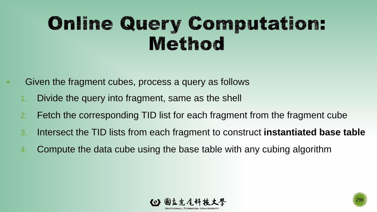
▪ Given the fragment cubes, process a query as follows
1. Divide the query into fragment, same as the shell
2. Fetch the corresponding TID list for each fragment from the fragment cube
3. Intersect the TID lists from each fragment to construct instantiated base table
4. Compute the data cube using the base table with any cubing algorithm
296
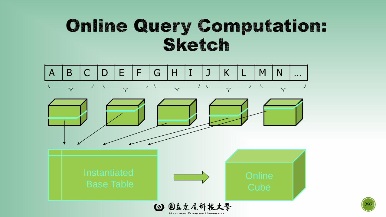
297
A B C D E F G H I J K L M N …
Online
Cube
Instantiated
Base Table
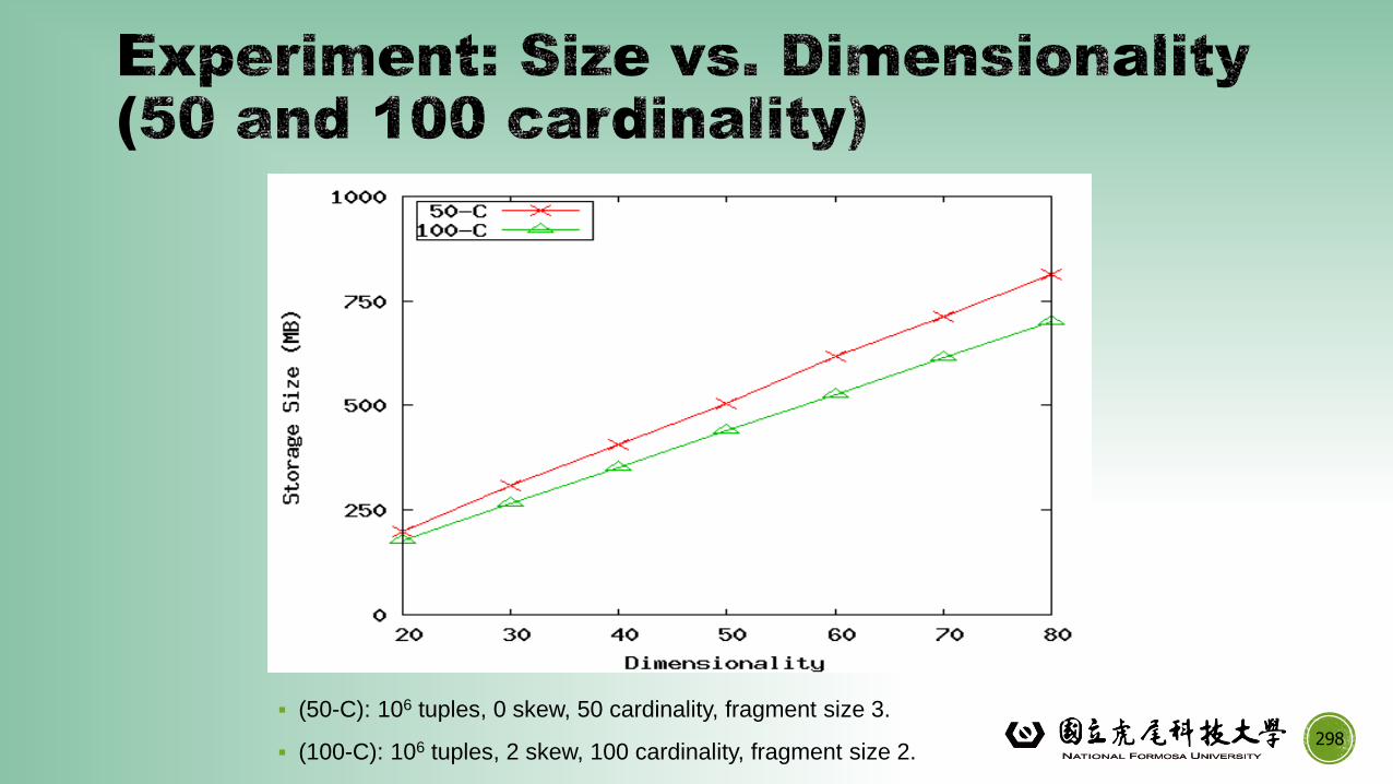
▪ (50-C): 106 tuples, 0 skew, 50 cardinality, fragment size 3.
▪ (100-C): 106 tuples, 2 skew, 100 cardinality, fragment size 2.298
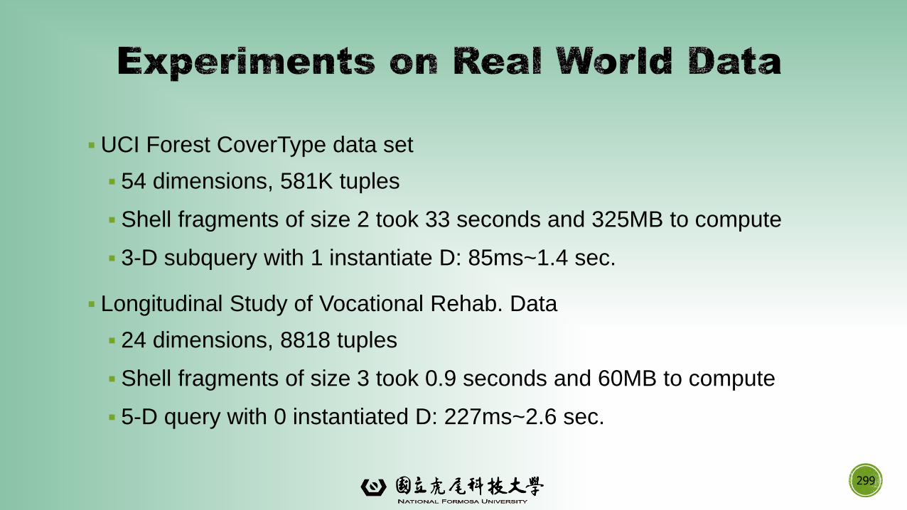
▪UCI Forest CoverType data set
▪ 54 dimensions, 581K tuples
▪ Shell fragments of size 2 took 33 seconds and 325MB to compute
▪ 3-D subquery with 1 instantiate D: 85ms~1.4 sec.
▪ Longitudinal Study of Vocational Rehab. Data
▪ 24 dimensions, 8818 tuples
▪ Shell fragments of size 3 took 0.9 seconds and 60MB to compute
▪ 5-D query with 0 instantiated D: 227ms~2.6 sec.
299
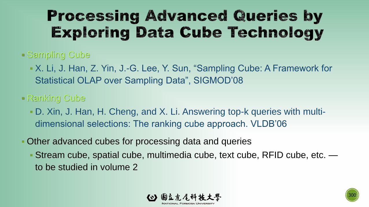
300
▪ Sampling Cube
▪ X. Li, J. Han, Z. Yin, J.-G. Lee, Y. Sun, “Sampling Cube: A Framework for
Statistical OLAP over Sampling Data”, SIGMOD’08
▪Ranking Cube
▪D. Xin, J. Han, H. Cheng, and X. Li. Answering top-k queries with multi-
dimensional selections: The ranking cube approach. VLDB’06
▪Other advanced cubes for processing data and queries
▪ Stream cube, spatial cube, multimedia cube, text cube, RFID cube, etc. —
to be studied in volume 2
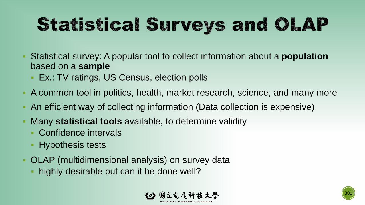
301
▪ Statistical survey: A popular tool to collect information about a populationbased on a sample
▪ Ex.: TV ratings, US Census, election polls
▪ A common tool in politics, health, market research, science, and many more
▪ An efficient way of collecting information (Data collection is expensive)
▪ Many statistical tools available, to determine validity
▪ Confidence intervals
▪ Hypothesis tests
▪ OLAP (multidimensional analysis) on survey data
▪ highly desirable but can it be done well?
302
▪ Data Mining Concepts and Techniques, 3rd ed