1

Deconstructing the Subprime Debacle Using New Indices of Underwriting Quality and Economic Conditions: A First Look1 

(Formerly titled: Subprime Mortgage Defaults, Loan Underwriting and Local Economic Conditions: A First Look) 

 

Charles D. Anderson,* Dennis R. Capozza** and Robert Van Order***

July 2008

Abstract

We document that technical progress in originating and pricing mortgages has enabled a trend since 1979 toward more relaxed credit standards on mortgage lending, which is reflected in rising foreclosure rates.  We then decompose annual variation in mortgage performance measured by share of loans entering foreclosure into a part due to economic conditions and a part due to underwriting changes. The decomposition provides natural metrics or indices of national underwriting quality and economic conditions. The results suggest that the recent subprime debacle can be attributed about equally to each factor. The deterioration since 1990 was marked by two periods. In the first, during the 1990s, there was a lowering of observable credit standards, like loan to value ratios.  It was deliberate and related to the use of credit scores and the development of more sophisticated underwriting systems. The negative effects of eroding loan quality on foreclosures were to some extent masked by strong local and national economic conditions during this period. In the second period, after 2002, there was little change in observable loan characteristics like loan to value or credit history. This second period is associated with the rise of subprime and Alt‐A markets but also with subprime and other “non‐agency” securitization. Securitization induced moral hazard and a deterioration in underwriting standards that was not easily observed by investors in the securities.  

*     University Financial Associates LLC (UFA) **   University of Michigan and UFA *** University of Aberdeen, University of Michigan, and UFA 

                                                            1 We thank Susan Wachter and the participants in seminars at the Homer Hoyt Advanced Studies Institute and the University of Michigan for helpful comments. The usual disclaimer applies.

  2

I. Introduction and Overview 

In this paper we document that technical progress in originating and pricing mortgages has

enabled a trend since 1979 toward more relaxed credit standards on mortgage lending, which is

reflected in rising foreclosure rates. We then decompose annual variation in mortgage

performance measured by share of loans entering foreclosure into a part due to economic

conditions and a part due to underwriting changes.

We find that the trend toward lower standards was characterized by two major periods of

deterioration, one in the middle and late 1990s and one after 2002. Our hypothesis is that in the

first period the change in credit standards was deliberate and well understood since it can be seen

in deterioration of readily measurable quality indicators, for instance an increase in the share of

low down payment loans in the loan mix. However, after 2002 there was little change in readily

observable indicators like credit score and loan-to-value. The change after 2002 can be better

attributed to an increase in moral hazard arising from securitization. Because of limitations in

our data set, we are painting with a rather broad brush. Our results are consistent with our

underlying hypotheses, but more detailed data will be required to eliminate other explanations.

We hypothesize that the pattern of losses including the recent sharp increase in defaults,

especially for subprime loans, arose from the interaction of technology in the form of credit

scoring and automated underwriting systems with a short look-back period for lenders and

investors for calibrating their new underwriting systems. These underwriting systems typically

did not incorporate the effects of changing local and national economic conditions. As a result,

when the short calibration period is economically favorable, lenders underestimate the baseline

hazard and misjudge the efficacy of their models. The opposite occurs when economic

conditions are unfavorable. This feedback pattern accentuates the credit cycle. Our metrics for

the economic environment for mortgage lending from 1990 to 2002 did indeed grow more

favorable each year; and in this environment lenders misjudged the default risks on mortgages,

especially subprime mortgages.

There was a second technological change in the years after 2000 that allowed for securitization

of subprime and other nontraditional loans. During this latter period there was a large increase in

the market share of non standard loans and a corresponding increase in mortgage-backed

  3

securities secured by such loans. Securitization of these non-standard loans separated the risk

bearing from the originator and enhanced moral hazard. This separation led to the second round

of “inadvertent” declines in underwriting quality. We show that while hard data like credit

scores and loan to value ratios did not erode during this period, there is indirect evidence that

“soft”2 data did erode. After about 2002 the favorable effects of the economic changes began to

reverse. Less favorable economic conditions, especially falling house prices, quickly exposed

the steep erosion in underwriting quality.

Our analysis in section III and IV uses the data from the Mortgage Bankers Association (MBA)

for foreclosures started each quarter on the stock of outstanding mortgages. We condition these

data for the serviced portfolio on metrics from University Financial Associates (UFA) that assess

the default risk arising from the local and national economic environment for each vintage in

each state. The year fixed effects from a regression of the MBA serviced portfolio data on lags

of the UFA local economic multipliers by vintage are a measure of the underwriting quality of

the serviced portfolio under the assumption that the UFA multipliers accurately assess the effects

of local and national economic conditions on defaults.

The fitted values from the regression minus the year fixed affects become the basis for an index

of how the economic environment at the local and national level is affecting foreclosures in the

serviced portfolio. The year fixed effects enable a corresponding index of underwriting quality.

The resulting patterns of the indices are consistent with the hypotheses outlined above. The

index for underwriting quality shows that absent the favorable economic environment,

foreclosure rates would have doubled from 1993 to 2004 rather than increasing the actual and

more modest 25%. We conjecture that indices like those developed in this research will be

invaluable to policy makers and investors when trying to assess risks in mortgage markets.

In section II we discuss basic facts of mortgage markets over time from different data sets. We

use these stylized facts to establish some general trends. In Section III we present our model. In

Section IV we present results. Section V summarizes and concludes.

                                                            2 We define “soft” data to be data that is not observable to the investor in the securitizations, although it may be known to the originator.

  4

II. Background and Summary Data: Stylized Facts 

Mortgage market data at the loan level, especially as they describe subprime and other

nontraditional loan types, are often proprietary. Here we discuss some aggregated results from

different sources to generate “stylized facts” that provide a context for our analysis in Section IV,

which uses a particular and limited data set.

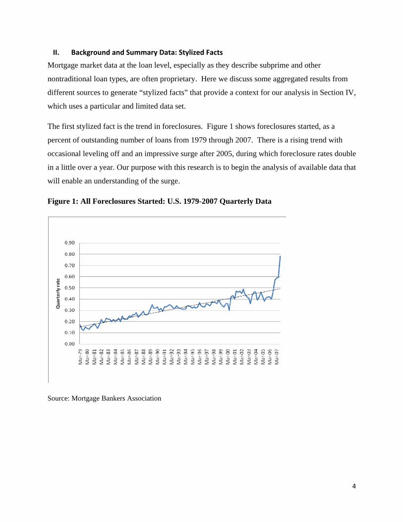
The first stylized fact is the trend in foreclosures. Figure 1 shows foreclosures started, as a

percent of outstanding number of loans from 1979 through 2007. There is a rising trend with

occasional leveling off and an impressive surge after 2005, during which foreclosure rates double

in a little over a year. Our purpose with this research is to begin the analysis of available data that

will enable an understanding of the surge.

Figure 1: All Foreclosures Started: U.S. 1979-2007 Quarterly Data

Source: Mortgage Bankers Association

  5

Credit Risk

There is a large literature on determinants of default risk in mortgage loans. Since the 1990s

many studies use data on borrower credit history along with more traditional data like loan to

value ratio, loan payment burden and economic performance. Credit history and credit scores,

which were originally developed by the Fair Isaac Corporation (FICO), and which use

proprietary models and data sets to determine the probability of making payments on consumer

credit for almost all adults in the U.S, have proven to be important explanatory variables.

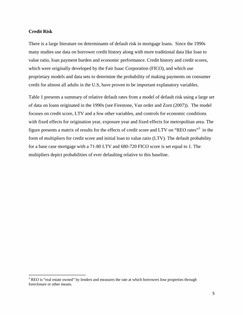
Table 1 presents a summary of relative default rates from a model of default risk using a large set

of data on loans originated in the 1990s (see Firestone, Van order and Zorn (2007)). The model

focuses on credit score, LTV and a few other variables, and controls for economic conditions

with fixed effects for origination year, exposure year and fixed effects for metropolitan area. The

figure presents a matrix of results for the effects of credit score and LTV on “REO rates”3 in the

form of multipliers for credit score and initial loan to value ratio (LTV). The default probability

for a base case mortgage with a 71-80 LTV and 680-720 FICO score is set equal to 1. The

multipliers depict probabilities of ever defaulting relative to this baseline.

                                                            3 REO is “real estate owned” by lenders and measures the rate at which borrowers lose properties through foreclosure or other means.

  6

Not that there is a nonlinear relationship among the variables; as LTV increases and credit score

decreases, foreclosure rates accelerate. Subprime loans are traditionally loans with credit scores below

620. History up to the period before the recent debacle suggested that subprime loans were indeed prone

to high default rates, especially if accompanied with low down payments. These results are consistent

with a wide range of more complicated research. They suggest not only that subprime loans are risky but

also that the consequences of misclassification are much higher in the subprime range. For example,

treating a loan that has a quality equivalent to a 650 credit score when it is really like a 600 has a much

bigger effect than mistaking a 700 for a 750. Hence, the consequences of manipulating the reporting of

hard data or unobservable “soft” data (see Keys et al., 2007) are likely to be bigger in the subprime

market.

House Prices

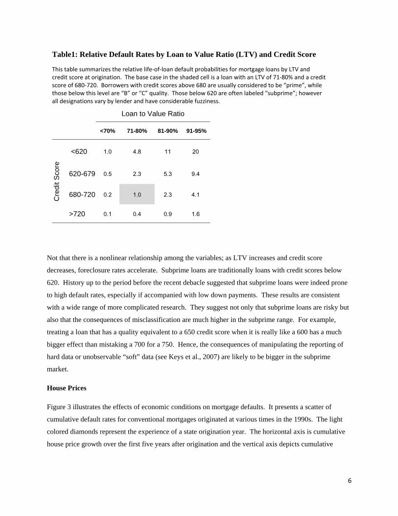
Figure 3 illustrates the effects of economic conditions on mortgage defaults. It presents a scatter of

cumulative default rates for conventional mortgages originated at various times in the 1990s. The light

colored diamonds represent the experience of a state origination year. The horizontal axis is cumulative

house price growth over the first five years after origination and the vertical axis depicts cumulative

Table1: Relative Default Rates by Loan to Value Ratio (LTV) and Credit Score

This table summarizes the relative life‐of‐loan default probabilities for mortgage loans by LTV and credit score at origination.  The base case in the shaded cell is a loan with an LTV of 71‐80% and a credit score of 680‐720.  Borrowers with credit scores above 680 are usually considered to be “prime”, while those below this level are “B” or “C” quality.  Those below 620 are often labeled “subprime”; however all designations vary by lender and have considerable fuzziness. 

Loan to Value Ratio

<70% 71-80% 81-90% 91-95%

Cre

dit S

core

<620 1.0 4.8 11 20

620-679 0.5 2.3 5.3 9.4

680-720 0.2 1.0 2.3 4.1

>720 0.1 0.4 0.9 1.6

 

  7

foreclosure (REO) rates over the first five years. All of the loans were 30 year fixed rate mortgages with

initial loan to value ratios close to 80%. There were no credit score data on these loans.

The shape of the scatter shows the important and nonlinear effect of house price growth on default. The

black squares represent the same experience but for the nationwide book by origination year. It shows the

(until recently) lack of a nationwide price decline and suggests benefits to nationwide diversification.

 Figure 3: Default Probability versus House Price Appreciation by Origination Year: The figure plots the cumulative default rates for 80% Loan-to-Value, 30-Year Fixed-Rate Home-Purchase Mortgages from 1985-1995 for both states and national data.

Table 1 and Figure 3 highlight the strong effects of basic measures of credit quality and economic

conditions. These data in various forms were available to subprime investors in the years after 2000.

They document that controlling for credit and LTV is important, and that while local economic conditions

mattered, diversified portfolios of mortgages had performed well.

Recent Performance by Product Type

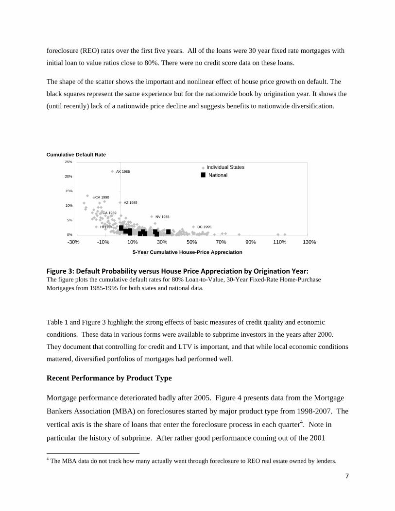
Mortgage performance deteriorated badly after 2005. Figure 4 presents data from the Mortgage

Bankers Association (MBA) on foreclosures started by major product type from 1998-2007. The

vertical axis is the share of loans that enter the foreclosure process in each quarter4. Note in

particular the history of subprime. After rather good performance coming out of the 2001

                                                            4 The MBA data do not track how many actually went through foreclosure to REO real estate owned by lenders.

 

NV 1985

HI 1994

AZ 1985

CA 1989

CA 1990

DC 1995

AK 1986

0% 

5% 

10% 

15% 

20% 

25% 

-30%  -10% 10% 30% 50% 70% 90% 110% 130%

5-Year Cumulative House-Price Appreciation

Cumulative Default Rate

Individual StatesNational

  8

recession foreclosures started increasing very sharply, especially for adjustable rate mortgages

(ARMs). A similar pattern but on a smaller scale occurs in the prime mortgage data, suggesting

that there is a common factor affecting both prime and subprime and that the surge in

foreclosures is not just a subprime issue.

Figure 4: Rate of Foreclosures started by loan type, 1998-2007 (%)

Source: Mortgage Bankers Association

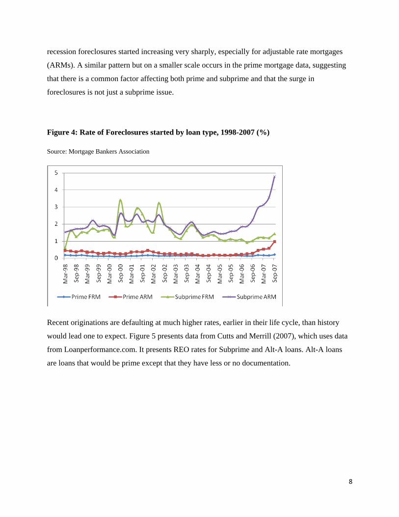
Recent originations are defaulting at much higher rates, earlier in their life cycle, than history

would lead one to expect. Figure 5 presents data from Cutts and Merrill (2007), which uses data

from Loanperformance.com. It presents REO rates for Subprime and Alt-A loans. Alt-A loans

are loans that would be prime except that they have less or no documentation.

  9

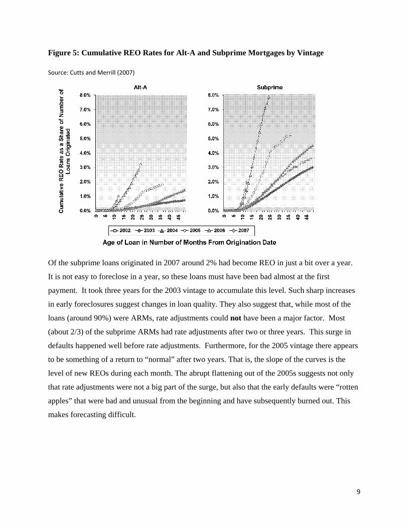
Figure 5: Cumulative REO Rates for Alt-A and Subprime Mortgages by Vintage

Source: Cutts and Merrill (2007) 

Of the subprime loans originated in 2007 around 2% had become REO in just a bit over a year.

It is not easy to foreclose in a year, so these loans must have been bad almost at the first

payment. It took three years for the 2003 vintage to accumulate this level. Such sharp increases

in early foreclosures suggest changes in loan quality. They also suggest that, while most of the

loans (around 90%) were ARMs, rate adjustments could not have been a major factor. Most

(about 2/3) of the subprime ARMs had rate adjustments after two or three years. This surge in

defaults happened well before rate adjustments. Furthermore, for the 2005 vintage there appears

to be something of a return to “normal” after two years. That is, the slope of the curves is the

level of new REOs during each month. The abrupt flattening out of the 2005s suggests not only

that rate adjustments were not a big part of the surge, but also that the early defaults were “rotten

apples” that were bad and unusual from the beginning and have subsequently burned out. This

makes forecasting difficult.

  10

Changes in Loan Characteristics

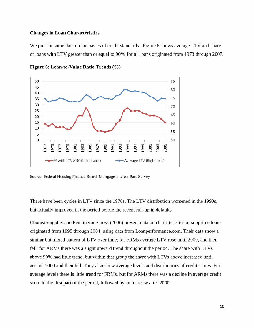
We present some data on the basics of credit standards. Figure 6 shows average LTV and share

of loans with LTV greater than or equal to 90% for all loans originated from 1973 through 2007.

Figure 6: Loan-to-Value Ratio Trends (%)

Source: Federal Housing Finance Board: Mortgage Interest Rate Survey

There have been cycles in LTV since the 1970s. The LTV distribution worsened in the 1990s,

but actually improved in the period before the recent run-up in defaults.

Chomsisengphet and Pennington-Cross (2006) present data on characteristics of subprime loans

originated from 1995 through 2004, using data from Loanperformance.com. Their data show a

similar but mixed pattern of LTV over time; for FRMs average LTV rose until 2000, and then

fell; for ARMs there was a slight upward trend throughout the period. The share with LTVs

above 90% had little trend, but within that group the share with LTVs above increased until

around 2000 and then fell. They also show average levels and distributions of credit scores. For

average levels there is little trend for FRMs, but for ARMs there was a decline in average credit

score in the first part of the period, followed by an increase after 2000.

  11

The distribution of credit scores was more complicated. The share of loans with very low credit

scores (below 500) dropped continuously throughout the period, from an initial level of around

70% to around 10% by 2004; the share between 500 and 600 increased in the first half of the

period and declined after 2000. Hence, there was a general trend from more lax standards on

credit and LTV in the late 1990s to generally tighter standards by 2004.

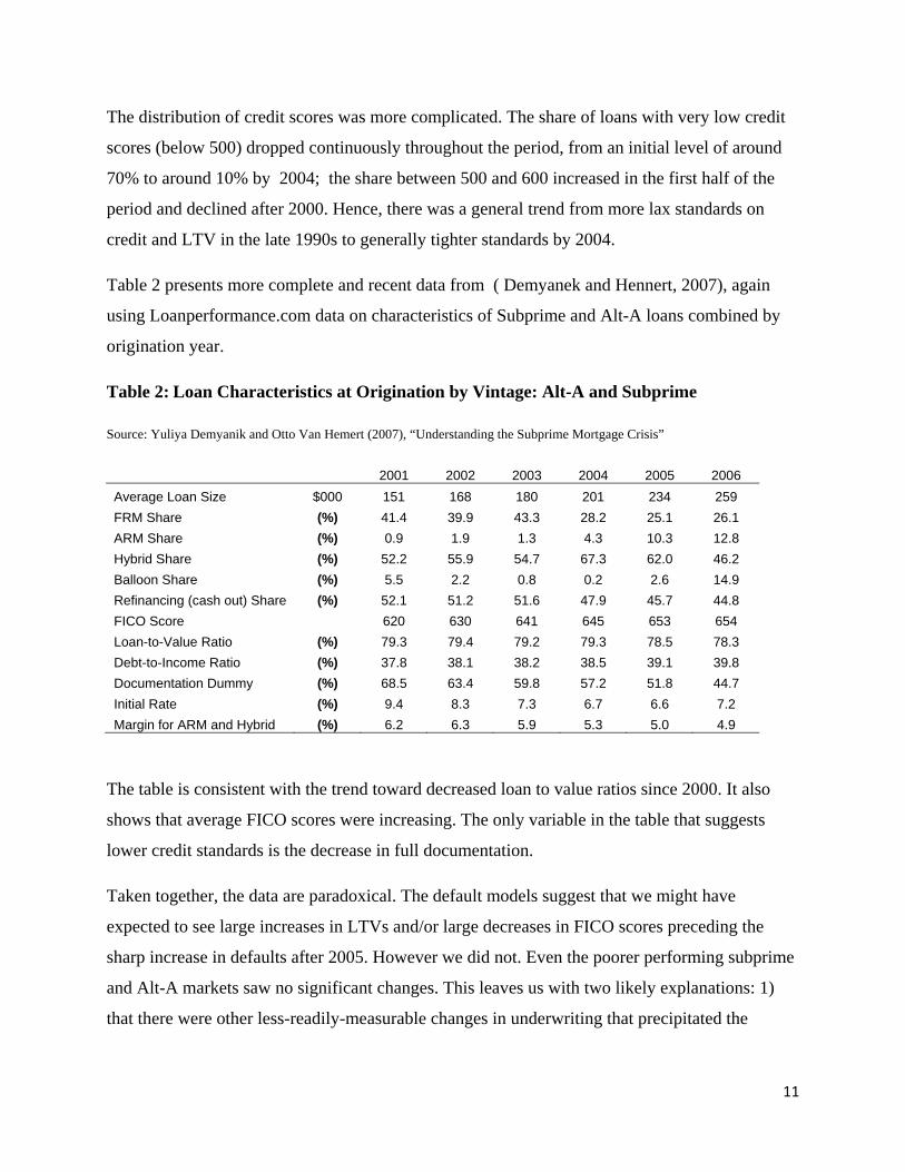
Table 2 presents more complete and recent data from ( Demyanek and Hennert, 2007), again

using Loanperformance.com data on characteristics of Subprime and Alt-A loans combined by

origination year.

Table 2: Loan Characteristics at Origination by Vintage: Alt-A and Subprime

Source: Yuliya Demyanik and Otto Van Hemert (2007), “Understanding the Subprime Mortgage Crisis”

2001 2002 2003 2004 2005 2006 Average Loan Size $000 151 168 180 201 234 259 FRM Share (%) 41.4 39.9 43.3 28.2 25.1 26.1 ARM Share (%) 0.9 1.9 1.3 4.3 10.3 12.8 Hybrid Share (%) 52.2 55.9 54.7 67.3 62.0 46.2 Balloon Share (%) 5.5 2.2 0.8 0.2 2.6 14.9 Refinancing (cash out) Share (%) 52.1 51.2 51.6 47.9 45.7 44.8 FICO Score 620 630 641 645 653 654 Loan-to-Value Ratio (%) 79.3 79.4 79.2 79.3 78.5 78.3 Debt-to-Income Ratio (%) 37.8 38.1 38.2 38.5 39.1 39.8 Documentation Dummy (%) 68.5 63.4 59.8 57.2 51.8 44.7 Initial Rate (%) 9.4 8.3 7.3 6.7 6.6 7.2 Margin for ARM and Hybrid (%) 6.2 6.3 5.9 5.3 5.0 4.9

The table is consistent with the trend toward decreased loan to value ratios since 2000. It also

shows that average FICO scores were increasing. The only variable in the table that suggests

lower credit standards is the decrease in full documentation.

Taken together, the data are paradoxical. The default models suggest that we might have

expected to see large increases in LTVs and/or large decreases in FICO scores preceding the

sharp increase in defaults after 2005. However we did not. Even the poorer performing subprime

and Alt-A markets saw no significant changes. This leaves us with two likely explanations: 1)

that there were other less-readily-measurable changes in underwriting that precipitated the

  12

change and/or 2) that economic conditions, especially the recent decline in property values, were

responsible.

Economic Conditions: The UFA Economic Multipliers and Risk Index

To assist in understanding the effects of local economic conditions we present an index produced

each quarter by University Financial Associates (UFA). UFA uses proprietary data on individual

subprime loans to estimate a competing hazards model of mortgage performance5. The model is

estimated from data on the characteristics of the loans, the properties and the borrower (credit

history, LTV etc.) as well as local economic conditions (house prices, employment etc.) The

UFA model is then used to create “multipliers” for local economic conditions by holding loan,

property and borrower characteristics constant and then allowing only the changes in local

economic conditions to affect mortgage performance. Essentially, this procedure takes a

constant quality loan and moves it around the country to see what impact local economies will

have on performance. It is not unusual to see four-fold or more differences in the default rates

on the constant quality loan as it travels virtually across the country. The UFA regional

multipliers are normalized so that the average is one each quarter.

The constant quality loan can also be applied to data in different years to create an index of how

quarterly economic conditions will affect mortgage performance. UFA creates such an index,

the UFA Default Risk Index, by aggregating the performance of the constant quality loan for

each loan vintage in each state to a national level index. The average performance of the 1990s

is set to 100 so that yearly values of the Index are relative to this baseline.

The UFA Regional Multipliers and Risk Index are especially useful in our modeling because

they provide summary statistics for local and annual economic conditions as they apply to

mortgage default, and will enable parsimonious estimation of the equations in Section IV. To

obtain the relative exposure to economic conditions over both time and space, we use the product

of the UFA Default Risk Index with the regional multipliers to obtain a metric for the regional

economic effects not normalized. We label this product the “UFA Economic Multipliers.”

                                                            5 For an early example of a default model with local economic conditions see Capozza, Kazarian and Thomson (1997)

  13

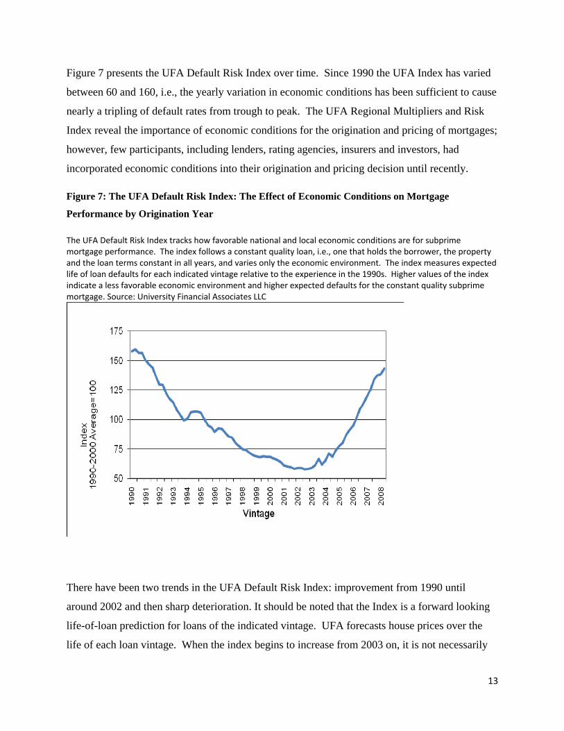
Figure 7 presents the UFA Default Risk Index over time. Since 1990 the UFA Index has varied

between 60 and 160, i.e., the yearly variation in economic conditions has been sufficient to cause

nearly a tripling of default rates from trough to peak. The UFA Regional Multipliers and Risk

Index reveal the importance of economic conditions for the origination and pricing of mortgages;

however, few participants, including lenders, rating agencies, insurers and investors, had

incorporated economic conditions into their origination and pricing decision until recently.

Figure 7: The UFA Default Risk Index: The Effect of Economic Conditions on Mortgage

Performance by Origination Year

The UFA Default Risk Index tracks how favorable national and local economic conditions are for subprime mortgage performance.  The index follows a constant quality loan, i.e., one that holds the borrower, the property and the loan terms constant in all years, and varies only the economic environment.  The index measures expected life of loan defaults for each indicated vintage relative to the experience in the 1990s.  Higher values of the index indicate a less favorable economic environment and higher expected defaults for the constant quality subprime mortgage. Source: University Financial Associates LLC 

There have been two trends in the UFA Default Risk Index: improvement from 1990 until

around 2002 and then sharp deterioration. It should be noted that the Index is a forward looking

life-of-loan prediction for loans of the indicated vintage. UFA forecasts house prices over the

life of each loan vintage. When the index begins to increase from 2003 on, it is not necessarily

  14

because the model expects the indicated vintage to default at high rates immediately. Any

increase during the life of the loan will affect the life-of-loan index value for that vintage. The

underlying UFA house price forecasts anticipated the current house price depreciation well in

advance and are incorporated into the Index. The figure suggests that indeed economic

conditions could be a major factor in explaining recent history.

Market Structure

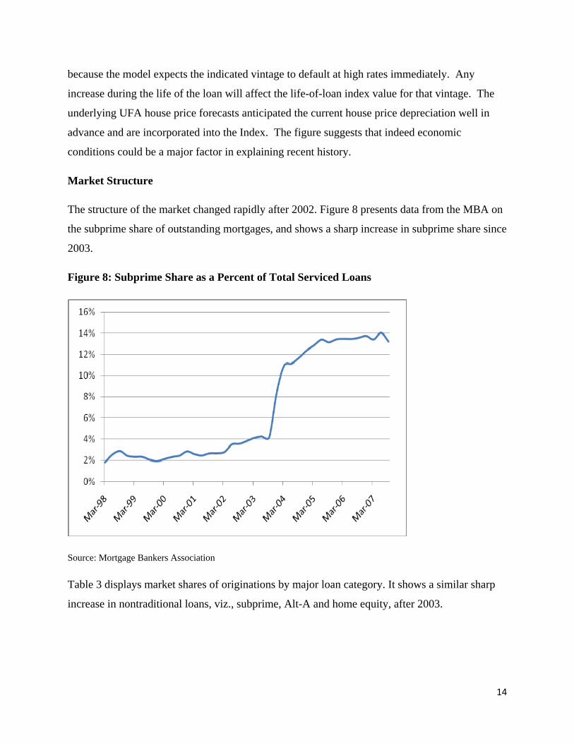
The structure of the market changed rapidly after 2002. Figure 8 presents data from the MBA on

the subprime share of outstanding mortgages, and shows a sharp increase in subprime share since

2003.

Figure 8: Subprime Share as a Percent of Total Serviced Loans

Source: Mortgage Bankers Association

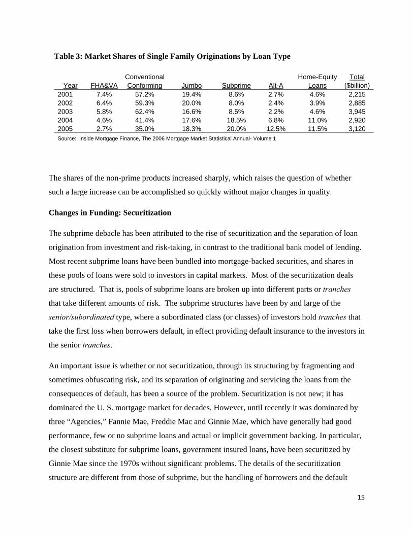
Table 3 displays market shares of originations by major loan category. It shows a similar sharp

increase in nontraditional loans, viz., subprime, Alt-A and home equity, after 2003.

  15

The shares of the non-prime products increased sharply, which raises the question of whether

such a large increase can be accomplished so quickly without major changes in quality.

Changes in Funding: Securitization

The subprime debacle has been attributed to the rise of securitization and the separation of loan

origination from investment and risk-taking, in contrast to the traditional bank model of lending.

Most recent subprime loans have been bundled into mortgage-backed securities, and shares in

these pools of loans were sold to investors in capital markets. Most of the securitization deals

are structured. That is, pools of subprime loans are broken up into different parts or tranches

that take different amounts of risk. The subprime structures have been by and large of the

senior/subordinated type, where a subordinated class (or classes) of investors hold tranches that

take the first loss when borrowers default, in effect providing default insurance to the investors in

the senior tranches.

An important issue is whether or not securitization, through its structuring by fragmenting and

sometimes obfuscating risk, and its separation of originating and servicing the loans from the

consequences of default, has been a source of the problem. Securitization is not new; it has

dominated the U. S. mortgage market for decades. However, until recently it was dominated by

three “Agencies,” Fannie Mae, Freddie Mac and Ginnie Mae, which have generally had good

performance, few or no subprime loans and actual or implicit government backing. In particular,

the closest substitute for subprime loans, government insured loans, have been securitized by

Ginnie Mae since the 1970s without significant problems. The details of the securitization

structure are different from those of subprime, but the handling of borrowers and the default

Table 3: Market Shares of Single Family Originations by Loan Type

Conventional Home-Equity Total Year FHA&VA Conforming Jumbo Subprime Alt-A Loans ($billion)

2001 7.4% 57.2% 19.4% 8.6% 2.7% 4.6% 2,215 2002 6.4% 59.3% 20.0% 8.0% 2.4% 3.9% 2,885 2003 5.8% 62.4% 16.6% 8.5% 2.2% 4.6% 3,945 2004 4.6% 41.4% 17.6% 18.5% 6.8% 11.0% 2,920 2005 2.7% 35.0% 18.3% 20.0% 12.5% 11.5% 3,120 Source: Inside Mortgage Finance, The 2006 Mortgage Market Statistical Annual- Volume 1

 

  16

process - a separate servicer who is not connected with the investors and who has no reason to be

nice to borrowers - is about the same. Despite the fact that subprime loans are more difficult to

securitize, their share has gone up.

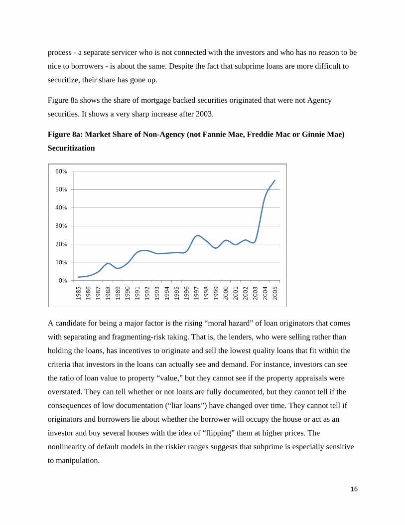
Figure 8a shows the share of mortgage backed securities originated that were not Agency

securities. It shows a very sharp increase after 2003.

Figure 8a: Market Share of Non-Agency (not Fannie Mae, Freddie Mac or Ginnie Mae)

Securitization

A candidate for being a major factor is the rising “moral hazard” of loan originators that comes

with separating and fragmenting-risk taking. That is, the lenders, who were selling rather than

holding the loans, has incentives to originate and sell the lowest quality loans that fit within the

criteria that investors in the loans can actually see and demand. For instance, investors can see

the ratio of loan value to property “value,” but they cannot see if the property appraisals were

overstated. They can tell whether or not loans are fully documented, but they cannot tell if the

consequences of low documentation (“liar loans”) have changed over time. They cannot tell if

originators and borrowers lie about whether the borrower will occupy the house or act as an

investor and buy several houses with the idea of “flipping” them at higher prices. The

nonlinearity of default models in the riskier ranges suggests that subprime is especially sensitive

to manipulation.

  17

Some recent work by Keys et al. (2007) presents indirect evidence of moral hazard. It appears

that 620 is a special credit score because loans with scores above 620 are more likely to be

eligible for Agency purchase. Historically credit scores have been a good predictor of default.

Keys et al. looked at loans just above and below 620. They controlled for a range of other

factors, but found that the loans just above 620 actually performed worse than those just below

620. Investors in pools can observe the hard data like credit score or LTV but not the soft data.

They conclude that the soft data were treated differently just above 620 in order to keep loans

eligible for Agency pools.

Summary and Hypotheses

To summarize the above data, we find that

• Foreclosure rates have been trending higher since at least 1979 when the MBA data start.

• LTV and credit scores are strong predictors of foreclosures; and the relation is highly

non-linear. Subprime loans with low credit scores and high LTVs can default at 20-200

times the rate of prime loans.

• House price appreciation is also a strong predictor; but until recently when local house

prices became synchronized, diversified pools were not greatly affected by regional

cycles like Texas in the 1980s.

• All product types have been affected by the recent surge in foreclosures but ARMs are

clearly worse than FRMs.

• Early performance of the 2005-2007 vintages has been extraordinarily bad in the first

year, ruling out resets, most of which occur after 2 or 3 years, as the source of the

problem.

• The evidence indicates that “hard” data like LTV and credit scores eroded in the 1990s,

but improved more recently. The erosion in underwriting quality occurred in the “soft”

data that was less readily available to investors in securitized pools.

• Improving national and local economic conditions supported the relaxed underwriting of

subprime loans until 2002. After 2002 there has been a steep erosion in local economic

  18

conditions, especially in real house price appreciation, which has turned negative in much

of the country.

• The market share of subprime and Alt-A loans rose dramatically after 2004.

• There was a corresponding increase in the securitization of these non-agency loans. The

share of non-agency securitizations nearly tripled after 2003; that is, securitizations

funded the increase in subprime originations.

The above stylized facts establish a clear rising trend in defaults, especially for subprime and

Alt-A loans. Two puzzles in the data are the increase in early defaults and the lack of

deterioration in common measures of credit quality, such as loan to value ratio and credit history.

Our hypothesis is that the diversification of pools and the favorable economic environment

masked the deterioration of loan quality in the middle and late 1990s. It induced investors to buy

the relatively high yielding but often highly rated pieces6 of subprime securities without much

analysis beyond the bond rating from the rating agencies. This invited moral hazard.

There were two important periods of diminished loan quality: one in the late 1990s, which was

deliberate and due to the development of scorecards and other innovations. This period saw a

decline in down payments and minimum credit scores; but the eroding loan quality was masked

by improving local economic conditions. In the second period after 2002, declining loan quality

may have been inadvertent in the sense that observables like credit score and down payment did

not change7, but quality declined nevertheless because unobservable factors (soft data) worsened.

The rise of loans with low or no documentation is consistent with this hypothesis. The evidence

in Section IV indicates that economic conditions, e.g., declining home prices, explain about half

of the increase in foreclosures started. However, the other half of the increase appears to be due

to changes in loan quality, which combined with the data suggesting no deterioration in

observable factors leads us to the moral hazard explanation.

                                                            6 Typically over 80% of a subprime pool had senior pieces with AAA ratings. 7 The Keys et al. study suggests that the decline in loan quality may not have been entirely inadvertent.

  19

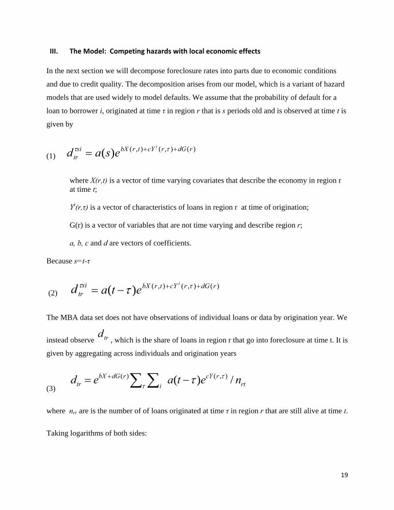
III. The Model:  Competing hazards with local economic effects 

In the next section we will decompose foreclosure rates into parts due to economic conditions

and due to credit quality. The decomposition arises from our model, which is a variant of hazard

models that are used widely to model defaults. We assume that the probability of default for a

loan to borrower i, originated at time τ in region r that is s periods old and is observed at time t is

given by

(1) )(),(),()( rdGrcYtrbXsi

tr

i

esad ++= ττ

where X(r,t) is a vector of time varying covariates that describe the economy in region r at time t;

Yi(r,τ) is a vector of characteristics of loans in region r at time of origination;

G(r) is a vector of variables that are not time varying and describe region r;

a, b, c and d are vectors of coefficients.

Because s=t-τ

(2) si

trd τ )(),(),()( rdGrcYtrbX i

eta ++−= ττ

The MBA data set does not have observations of individual loans or data by origination year. We

instead observe trd, which is the share of loans in region r that go into foreclosure at time t. It is

given by aggregating across individuals and origination years

(3) rtrcY

irdGbX

tr netaed /)( ),()( ττ

τ−= ∑ ∑+

where nrt are is the number of of loans originated at time τ in region r that are still alive at time t.

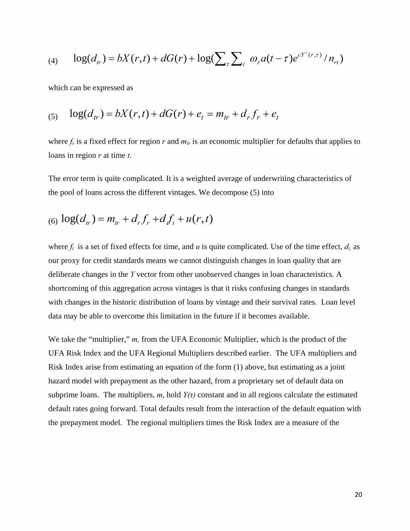
Taking logarithms of both sides:

  20

(4) )/)(log()(),()log( ),(rt

rcYitr netardGtrbXd

i ττ τ τω −++= ∑ ∑

which can be expressed as

(5) trrtrttr efdmerdGtrbXd ++=++= )(),()log(

where fr is a fixed effect for region r and mtr is an economic multiplier for defaults that applies to

loans in region r at time t.

The error term is quite complicated. It is a weighted average of underwriting characteristics of

the pool of loans across the different vintages. We decompose (5) into

(6) ),()log( trufdfdmd ttrrtrtr +++=

where ft is a set of fixed effects for time, and u is quite complicated. Use of the time effect, dt, as

our proxy for credit standards means we cannot distinguish changes in loan quality that are

deliberate changes in the Y vector from other unobserved changes in loan characteristics. A

shortcoming of this aggregation across vintages is that it risks confusing changes in standards

with changes in the historic distribution of loans by vintage and their survival rates. Loan level

data may be able to overcome this limitation in the future if it becomes available.

We take the “multiplier,” m, from the UFA Economic Multiplier, which is the product of the

UFA Risk Index and the UFA Regional Multipliers described earlier. The UFA multipliers and

Risk Index arise from estimating an equation of the form (1) above, but estimating as a joint

hazard model with prepayment as the other hazard, from a proprietary set of default data on

subprime loans. The multipliers, m, hold Y(τ) constant and in all regions calculate the estimated

default rates going forward. Total defaults result from the interaction of the default equation with

the prepayment model. The regional multipliers times the Risk Index are a measure of the

  21

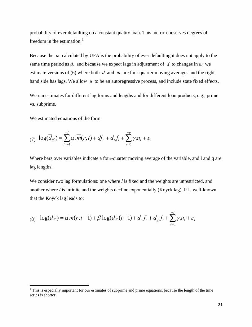
probability of ever defaulting on a constant quality loan. This metric conserves degrees of

freedom in the estimation.8

Because the m calculated by UFA is the probability of ever defaulting it does not apply to the

same time period as d, and because we expect lags in adjustment of d to changes in m, we

estimate versions of (6) where both d and m are four quarter moving averages and the right

hand side has lags. We allow u to be an autoregressive process, and include state fixed effects.

We ran estimates for different lag forms and lengths and for different loan products, e.g., prime

vs. subprime.

We estimated equations of the form

(7) tt

q

ttttr

l

tttr ufddftrmd εγα ++++= ∑∑

−

=

−

−= 01),()log(

Where bars over variables indicate a four-quarter moving average of the variable, and l and q are

lag lengths.

We consider two lag formulations: one where l is fixed and the weights are unrestricted, and

another where l is infinite and the weights decline exponentially (Koyck lag). It is well-known

that the Koyck lag leads to:

(8) tt

l

tttfrrtrtr ufdfdtdtrmd εγβα ++++−+−= ∑

−

=0)1(log()1,()log(

                                                            8 This is especially important for our estimates of subprime and prime equations, because the length of the time series is shorter.

  22

IV. Results: The relative roles of economic conditions and moral hazard

We use data from the Mortgage Bankers Association (like those in Figures 1, 4 and 8) along with

the UFA Economic Multipliers to model foreclosure rates state by state. Our data set is a panel.

On the left hand side we have (log of) foreclosure rates by quarter and by state from the MBA

survey, and on the right hand side we have the (log of) the UFA Economic Multipliers for local

economic conditions by quarter and by state. Our maintained hypothesis is that the slopes are

constant across states and time, but there are separate constant terms for each state and time

effects, which do not change across states. We estimate variants of (7) and (8) and use the

estimated equations to simulate the separate effects of the multipliers, m, and the time fixed

effects, D(t), on foreclosure rates over time. There are versions for all loans and for prime and

subprime separately.

We present two versions of our model (without showing the fixed effects). The first, Model 1, is

equation (7) with four quarter moving averages and four yearly lags for the UFA multipliers with

no restrictions on the lags. The second, Model 2, has a geometrically distributed (Koyck) lag,

equation (8), with the first lagged UFA multiplier and the lagged dependent variable on the right

hand side. We also present versions by loan type: prime vs subprime. Time periods vary because

the data were not recorded separately for prime and subprime until 1998. Table 5 presents

estimates of Model 1 and Table 6 has results for Model 2.

  23

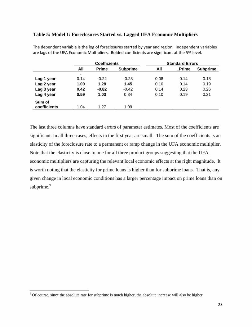
The last three columns have standard errors of parameter estimates. Most of the coefficients are

significant. In all three cases, effects in the first year are small. The sum of the coefficients is an

elasticity of the foreclosure rate to a permanent or ramp change in the UFA economic multiplier.

Note that the elasticity is close to one for all three product groups suggesting that the UFA

economic multipliers are capturing the relevant local economic effects at the right magnitude. It

is worth noting that the elasticity for prime loans is higher than for subprime loans. That is, any

given change in local economic conditions has a larger percentage impact on prime loans than on

subprime.9

                                                            9 Of course, since the absolute rate for subprime is much higher, the absolute increase will also be higher.

Table 5: Model 1: Foreclosures Started vs. Lagged UFA Economic Multipliers

The dependent variable is the log of foreclosures started by year and region.  Independent variables are lags of the UFA Economic Multipliers.  Bolded coefficients are significant at the 5% level. 

Coefficients

Standard Errors All Prime Subprime All _Prime Subprime

Lag 1 year -

0.14 -0.22 -0.28

0.08 0.14 0.18 Lag 2 year 1.00 1.28 1.45 0.10 0.14 0.19 Lag 3 year 0.42 -0.82 -0.42 0.14 0.23 0.26 Lag 4 year 0.59 1.03 0.34 0.10 0.19 0.21

Sum of coefficients 1.04 1.27 1.09

  24

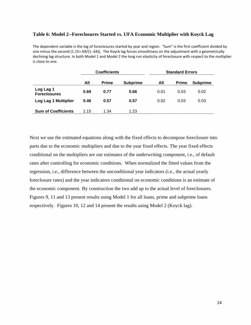
Next we use the estimated equations along with the fixed effects to decompose foreclosure into

parts due to the economic multipliers and due to the year fixed effects. The year fixed effects

conditional on the multipliers are our estimates of the underwriting component, i.e., of default

rates after controlling for economic conditions. When normalized the fitted values from the

regression, i.e., difference between the unconditional year indicators (i.e., the actual yearly

foreclosure rates) and the year indicators conditional on economic conditions is an estimate of

the economic component. By construction the two add up to the actual level of foreclosures.

Figures 9, 11 and 13 present results using Model 1 for all loans, prime and subprime loans

respectively. Figures 10, 12 and 14 present the results using Model 2 (Koyck lag).

Table 6: Model 2--Foreclosures Started vs. UFA Economic Multiplier with Koyck Lag

The dependent variable is the log of foreclosures started by year and region.  “Sum” is the first coefficient divided by one minus the second (1.15=.69/(1‐.64)).  The Koyck lag forces smoothness on the adjustment with a geometrically declining lag structure. In both Model 1 and Model 2 the long run elasticity of foreclosure with respect to the multiplier is close to one. 

Coefficients

Standard Errors

All Prime Subprime

All Prime Subprime Log Lag 1 Foreclosures 0.69 0.77 0.66 0.01 0.03 0.02

Log Lag 1 Multiplier 0.46 0.57 0.57 0.02 0.03 0.03 Sum of Coefficients 1.15 1.34 1.23

 

  25

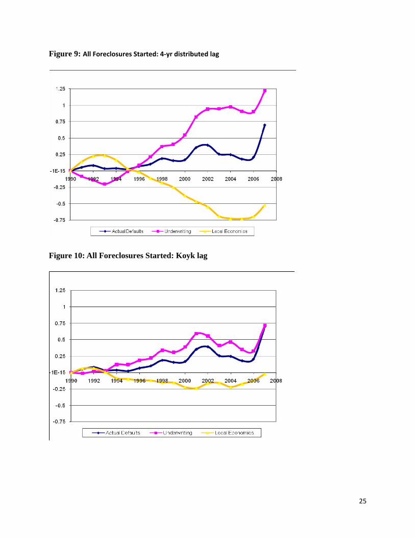
Figure 9: All Foreclosures Started: 4‐yr distributed lag 

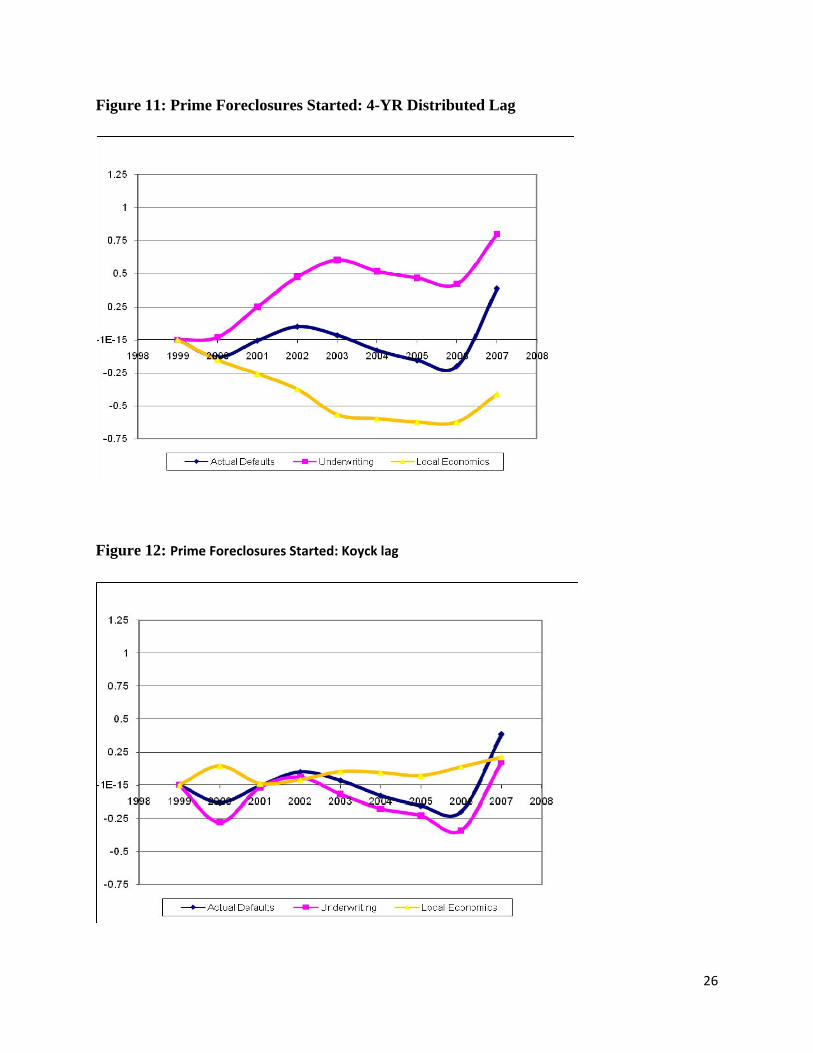
Figure 10: All Foreclosures Started: Koyk lag

  26

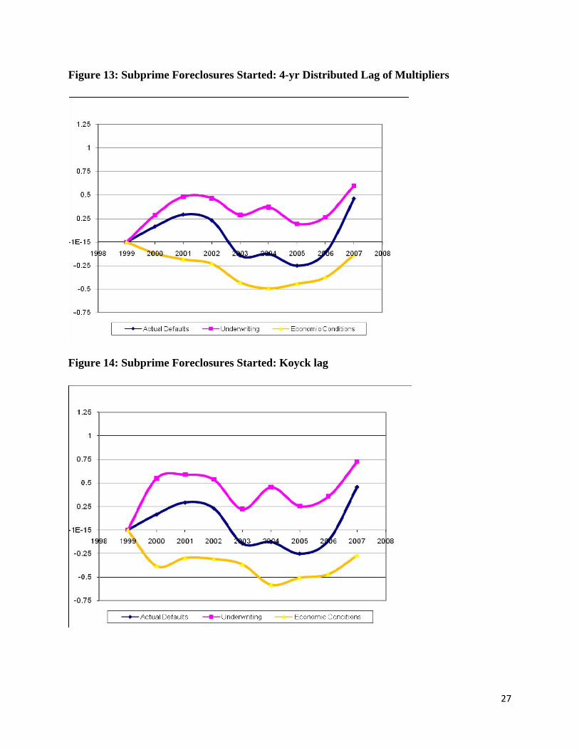
Figure 11: Prime Foreclosures Started: 4-YR Distributed Lag

Figure 12: Prime Foreclosures Started: Koyck lag 

  27

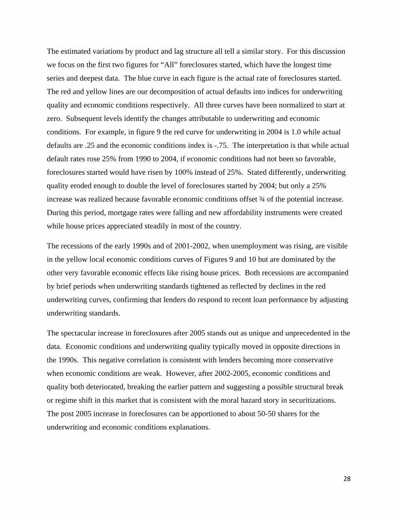
Figure 13: Subprime Foreclosures Started: 4-yr Distributed Lag of Multipliers

Figure 14: Subprime Foreclosures Started: Koyck lag

  28

The estimated variations by product and lag structure all tell a similar story. For this discussion

we focus on the first two figures for “All” foreclosures started, which have the longest time

series and deepest data. The blue curve in each figure is the actual rate of foreclosures started.

The red and yellow lines are our decomposition of actual defaults into indices for underwriting

quality and economic conditions respectively. All three curves have been normalized to start at

zero. Subsequent levels identify the changes attributable to underwriting and economic

conditions. For example, in figure 9 the red curve for underwriting in 2004 is 1.0 while actual

defaults are .25 and the economic conditions index is -.75. The interpretation is that while actual

default rates rose 25% from 1990 to 2004, if economic conditions had not been so favorable,

foreclosures started would have risen by 100% instead of 25%. Stated differently, underwriting

quality eroded enough to double the level of foreclosures started by 2004; but only a 25%

increase was realized because favorable economic conditions offset ¾ of the potential increase.

During this period, mortgage rates were falling and new affordability instruments were created

while house prices appreciated steadily in most of the country.

The recessions of the early 1990s and of 2001-2002, when unemployment was rising, are visible

in the yellow local economic conditions curves of Figures 9 and 10 but are dominated by the

other very favorable economic effects like rising house prices. Both recessions are accompanied

by brief periods when underwriting standards tightened as reflected by declines in the red

underwriting curves, confirming that lenders do respond to recent loan performance by adjusting

underwriting standards.

The spectacular increase in foreclosures after 2005 stands out as unique and unprecedented in the

data. Economic conditions and underwriting quality typically moved in opposite directions in

the 1990s. This negative correlation is consistent with lenders becoming more conservative

when economic conditions are weak. However, after 2002-2005, economic conditions and

quality both deteriorated, breaking the earlier pattern and suggesting a possible structural break

or regime shift in this market that is consistent with the moral hazard story in securitizations.

The post 2005 increase in foreclosures can be apportioned to about 50-50 shares for the

underwriting and economic conditions explanations.

  29

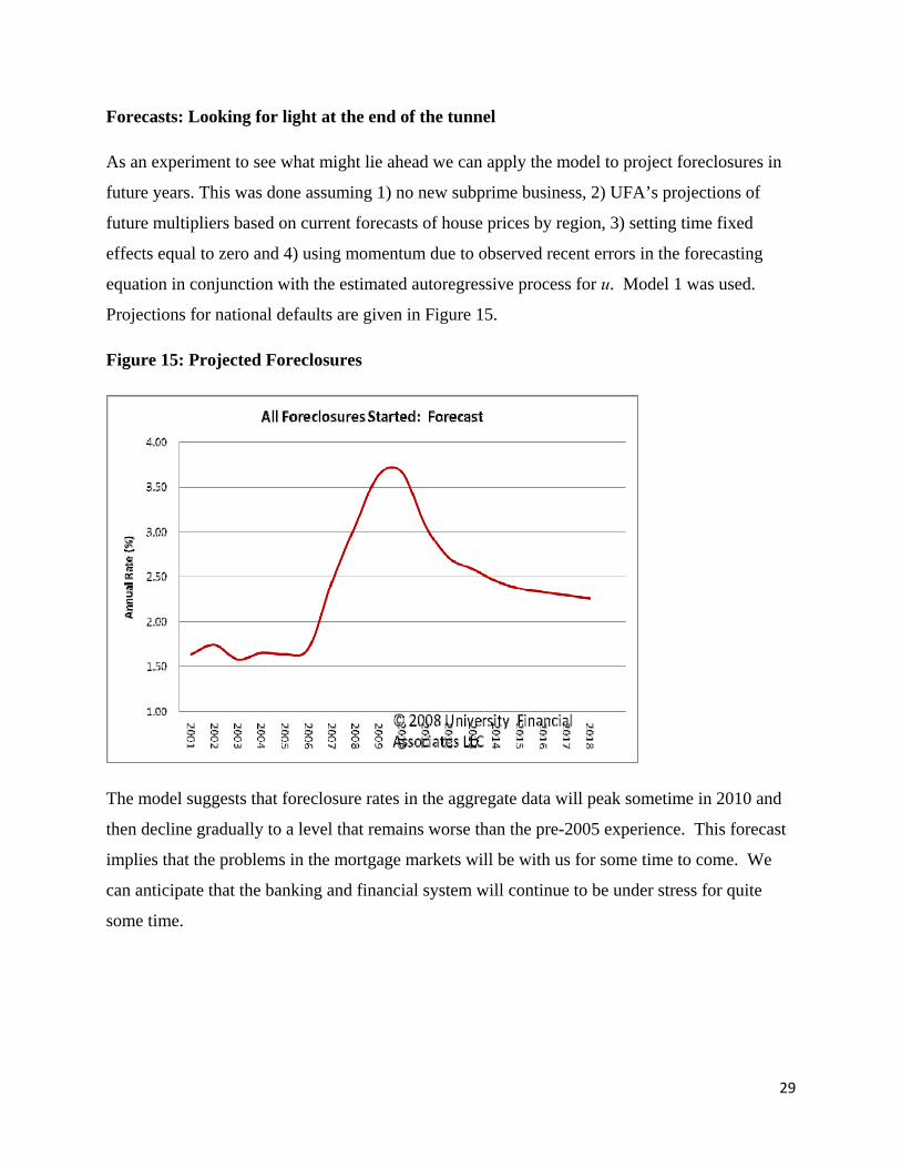
Forecasts: Looking for light at the end of the tunnel

As an experiment to see what might lie ahead we can apply the model to project foreclosures in

future years. This was done assuming 1) no new subprime business, 2) UFA’s projections of

future multipliers based on current forecasts of house prices by region, 3) setting time fixed

effects equal to zero and 4) using momentum due to observed recent errors in the forecasting

equation in conjunction with the estimated autoregressive process for u. Model 1 was used.

Projections for national defaults are given in Figure 15.

Figure 15: Projected Foreclosures

The model suggests that foreclosure rates in the aggregate data will peak sometime in 2010 and

then decline gradually to a level that remains worse than the pre-2005 experience. This forecast

implies that the problems in the mortgage markets will be with us for some time to come. We

can anticipate that the banking and financial system will continue to be under stress for quite

some time.

  30

IV. Comments and Conclusions

We document the long standing deterioration in foreclosure rates since 1979 that was marked by

two periods. The first was accompanied by a lowering of standards like loan to value ratios in

the 1990s. The second change, which was not seen in observable loan characteristics like down

payment and credit history, was associated with the rise of the subprime market and non-agency

securitization.

The surge in defaults after 2005, especially subprime defaults, was undoubtedly the result of

several factors happening at once. The performance history of the 1990s had suggested that

subprime performance was tolerable, that credit score and LTV based underwriting models

worked well and that nationally diversified pools of mortgages were safe. This made extending

securitization into this new area look promising. However, the favorable economic conditions of

the 1990s made subprime look better than the reality. When economic conditions reversed after

2002, diversified pools were not of much help with house prices falling in most of the country.

At the same time, securitization invited moral hazard, particularly in ways that credit scores and

LTV could not detect.

In the empirical analysis, we decomposed the deterioration in mortgage performance into parts

due to weakened economic conditions and to underwriting changes. Our results suggest about a

50-50 split between the looser underwriting and unfavorable economic conditions explanations

for the recent surge in foreclosures. The model and empirical analysis enable us to create indices

of both underwriting quality and economic conditions for mortgage loans. These indices should

be valuable to policy makers and investors who wish to monitor or assess the risks in mortgage

pools and mortgage markets.

Our empirical results are consistent with the underlying hypotheses, but more detailed data will

be required to eliminate other explanations. While we get similar results for prime loans, it is not

clear what to make of them because our data do not separate Alt-A from other prime loans.10

There are data that suggest that Alt A, though not as bad as subprime, performed much worse

than other prime loans.

                                                            10 Note that our estimates are all in logs, so similar coefficients means similar multiplier effects, but subprime and Alt-A are much larger numbers to begin with, so their effects in levels are much bigger.

  31

REFERENCES

Capozza D, Kazarian and Thomson, “Mortgage Default in Local Markets,” Real Estate Economics, (1997)

Chomsisengphet, S. and A Pennington- Cross, “The Evolution of the Subprime Mortgage Market.” Federal Reserve Bank of St. Louis Review, January/February 2006, 88(1), pp. 31-56.

Cutts, A and W. Merrill, “Interventions in Mortgage Default: Policies and Practices to Prevent Home Loss and Lower Costs.” Mimeo (2007)

Demyanyk, Yuliya and Otto Van Hemert, “Understanding the Subprime Mortgage Crisis” Mimeo (2007)

Firestone, S, R Van Order and P Zorn “Performance of Low Income and Minority Loans,” Real Estate Economics, (2007)

Keys, B, t. Mukerjee, A. Seru, and V. Vig. “Securities and Screening: Evidence from Sub Prime Mortgage-Backed Securities.” Mimeo (2007)