DirectLiNGAM:A direct estimation method for

LiNGAM

Shohei Shimizu, Takanori Inazumi, Yasuhiro Sogawa, Osaka Univ.Aapo Hyvarinen, Univ. HelsinkiYoshinobu Kawahara, Takashi Washio, Osaka Univ.Patrik O. Hoyer, Univ. HelsinkiKenneth Bollen, Univ. North Carolina

Updated at Jan 14 2011

2

Abstract

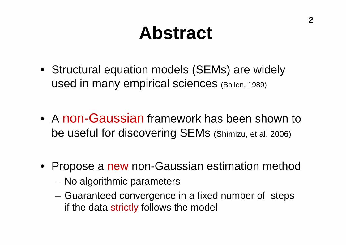
• Structural equation models (SEMs) are widely used in many empirical sciences (Bollen, 1989)

• A non-Gaussian framework has been shown to be useful for discovering SEMs (Shimizu, et al. 2006)

• Propose a new non-Gaussian estimation method– No algorithmic parameters– Guaranteed convergence in a fixed number of steps

if the data strictly follows the model

Background

4Linear Non-Gaussian Acyclic Model

(LiNGAM model) (Shimizu et al. 2006)

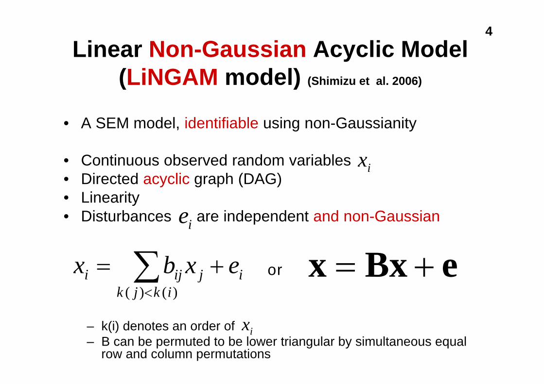
• A SEM model, identifiable using non-Gaussianity

• Continuous observed random variables • Directed acyclic graph (DAG)• Linearity• Disturbances are independent and non-Gaussian

– k(i) denotes an order of– B can be permuted to be lower triangular by simultaneous equal

row and column permutations

eBxx +=iikjk

jiji exbx += ∑< )()(

or

ix

ie

ix

5

-1.3

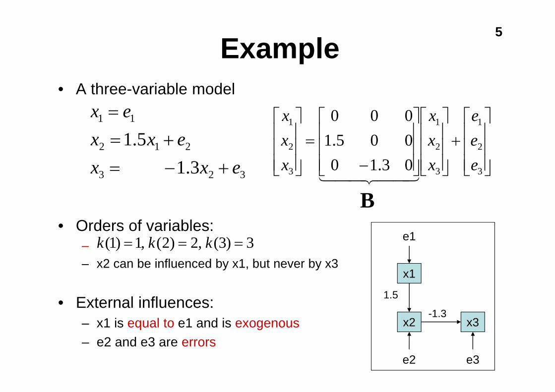
Example• A three-variable model

• Orders of variables:–– x2 can be influenced by x1, but never by x3

• External influences:– x1 is equal to e1 and is exogenous– e2 and e3 are errors

323

212

11

3.15.1

exxexx

ex

+−=+=

=

⎥⎥⎥

⎦

⎤

⎢⎢⎢

⎣

⎡+

⎥⎥⎥

⎦

⎤

⎢⎢⎢

⎣

⎡

⎥⎥⎥

⎦

⎤

⎢⎢⎢

⎣

⎡

−=

⎥⎥⎥

⎦

⎤

⎢⎢⎢

⎣

⎡

3

2

1

3

2

1

3

2

1

03.10005.1000

eee

xxx

xxx

44 344 21

3)3(,2)2(,1)1( === kkk

x3

x1

x2

1.5

e1

e2 e3

B

6

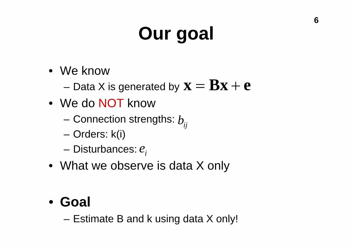
Our goal

• We know– Data X is generated by

• We do NOT know– Connection strengths: – Orders: k(i)– Disturbances:

• What we observe is data X only

• Goal– Estimate B and k using data X only!

eBxx +=

ie

ijb

Previous work

8Independent Component Analysis(Comon 1994; Hyvarinen et al., 2001)

• A is an unknown square matrix• are independent and non-Gaussian

• Identifiable including the rotation (Comon, 1994)

• Many estimation methods– e.g., FastICA (Hyvarinen,99), Amari (99) and Bach & Jordan (02)

Asx =

is

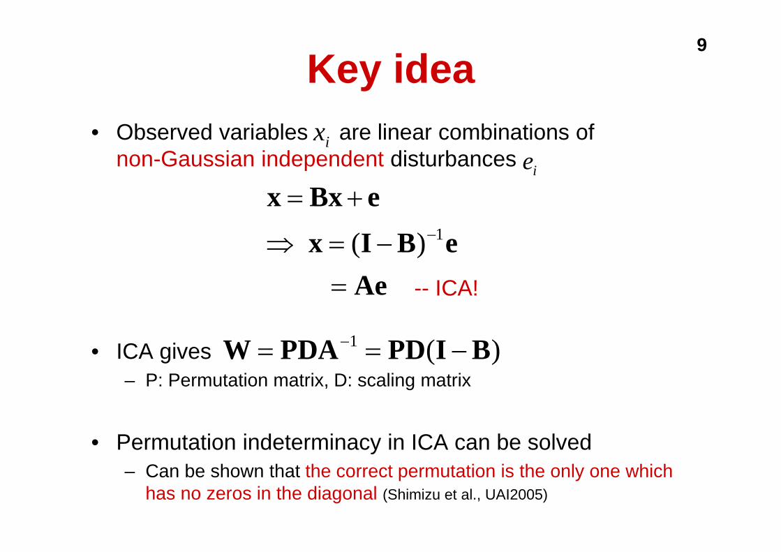
9Key idea

• Observed variables are linear combinations of non-Gaussian independent disturbances

• ICA gives – P: Permutation matrix, D: scaling matrix

• Permutation indeterminacy in ICA can be solved– Can be shown that the correct permutation is the only one which

has no zeros in the diagonal (Shimizu et al., UAI2005)

AeeBIx

eBxx

=−=⇒

+=−1)(

ixie

)(1 BIPDPDAW −== −

-- ICA!

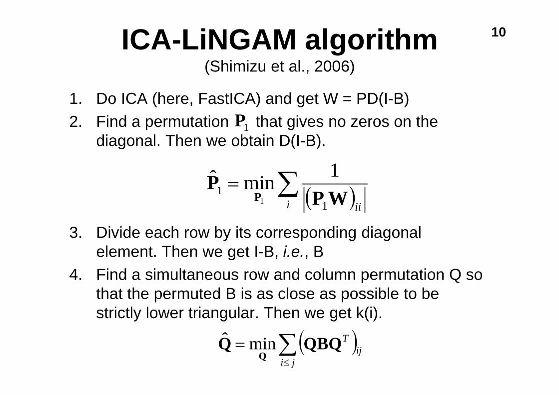
10ICA-LiNGAM algorithm(Shimizu et al., 2006)

1. Do ICA (here, FastICA) and get W = PD(I-B)2. Find a permutation that gives no zeros on the

diagonal. Then we obtain D(I-B).

3. Divide each row by its corresponding diagonal element. Then we get I-B, i.e., B

4. Find a simultaneous row and column permutation Q so that the permuted B is as close as possible to be strictly lower triangular. Then we get k(i).

( )∑=i iiWP

PP

11

1minˆ1

( )∑≤

=ji

ijTQBQQ

Qminˆ

1P

11

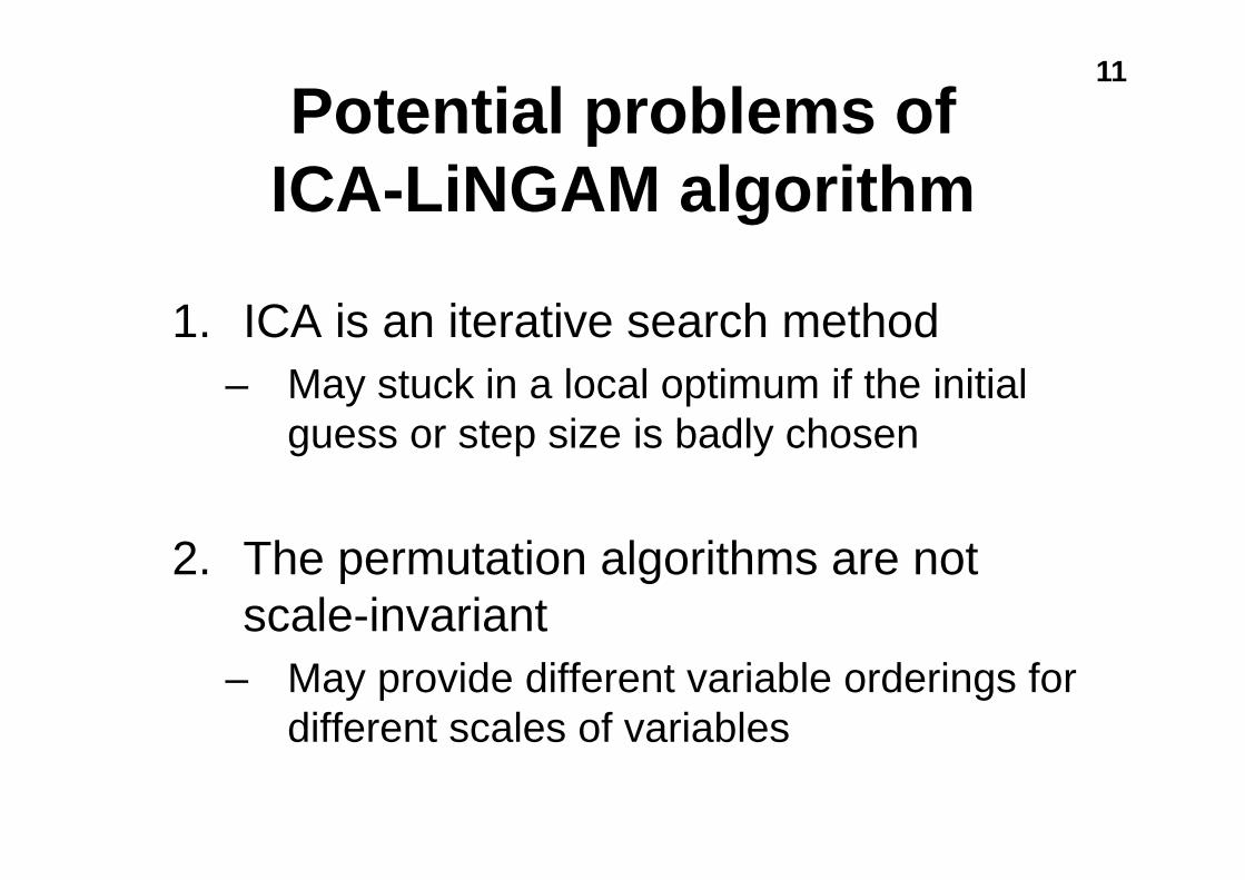
Potential problems of ICA-LiNGAM algorithm

1. ICA is an iterative search method– May stuck in a local optimum if the initial

guess or step size is badly chosen

2. The permutation algorithms are not scale-invariant

– May provide different variable orderings for different scales of variables

A new method

13

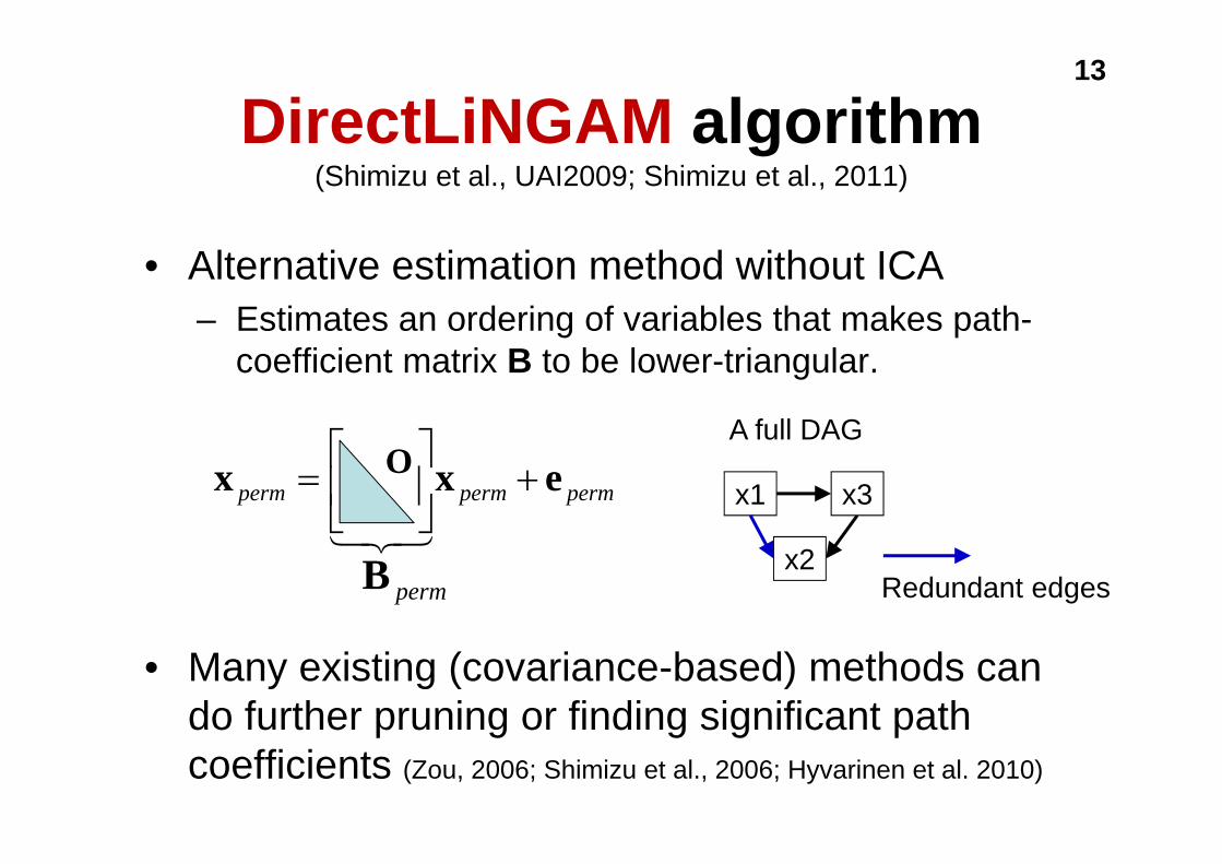
DirectLiNGAM algorithm(Shimizu et al., UAI2009; Shimizu et al., 2011)

• Alternative estimation method without ICA– Estimates an ordering of variables that makes path-

coefficient matrix B to be lower-triangular.

• Many existing (covariance-based) methods can do further pruning or finding significant path coefficients (Zou, 2006; Shimizu et al., 2006; Hyvarinen et al. 2010)

permpermperm exx +⎥⎦

⎤⎢⎣

⎡=

321

permB

O

x2

x3x1

Redundant edges

A full DAG

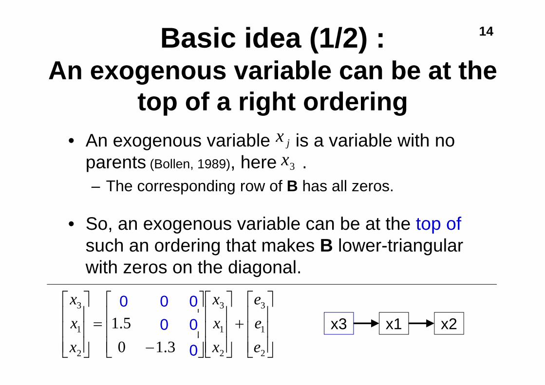
14Basic idea (1/2) : An exogenous variable can be at the

top of a right ordering • An exogenous variable is a variable with no

parents (Bollen, 1989), here .– The corresponding row of B has all zeros.

• So, an exogenous variable can be at the top ofsuch an ordering that makes B lower-triangular with zeros on the diagonal.

⎥⎥⎥

⎦

⎤

⎢⎢⎢

⎣

⎡+

⎥⎥⎥

⎦

⎤

⎢⎢⎢

⎣

⎡

⎥⎥⎥

⎦

⎤

⎢⎢⎢

⎣

⎡

−=

⎥⎥⎥

⎦

⎤

⎢⎢⎢

⎣

⎡

2

1

3

2

1

3

2

1

3

03.10005.1000

eee

xxx

xxx

0000

00x3 x1 x2

jx3x

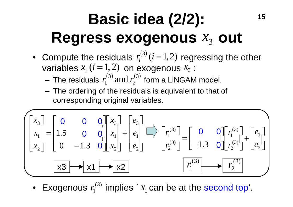
15Basic idea (2/2): Regress exogenous out

• Compute the residuals regressing the other variables on exogenous :– The residuals form a LiNGAM model. – The ordering of the residuals is equivalent to that of

corresponding original variables.

• Exogenous implies ` can be at the second top’.)3(1r 1x

3x( ) )2,1(3 =iri

3x)2,1( =ixi

⎥⎥⎥

⎦

⎤

⎢⎢⎢

⎣

⎡+

⎥⎥⎥

⎦

⎤

⎢⎢⎢

⎣

⎡

⎥⎥⎥

⎦

⎤

⎢⎢⎢

⎣

⎡

−=

⎥⎥⎥

⎦

⎤

⎢⎢⎢

⎣

⎡

2

1

3

2

1

3

2

1

3

03.10005.1000

eee

xxx

xxx 0

00 0

00

00

⎥⎦

⎤⎢⎣

⎡+⎥

⎦

⎤⎢⎣

⎡⎥⎦

⎤⎢⎣

⎡−

=⎥⎦

⎤⎢⎣

⎡

2

1)3(

2

)3(1

)3(2

)3(1

03.100

ee

rr

rr 0 0

)3(2r

)3(1rx3 x1 x2

( ) ( )32

31 and rr

0

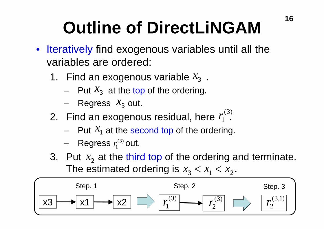
16

• Iteratively find exogenous variables until all the variables are ordered:1. Find an exogenous variable .

– Put at the top of the ordering. – Regress out.

2. Find an exogenous residual, here .– Put at the second top of the ordering.– Regress out.

3. Put at the third top of the ordering and terminate. The estimated ordering is

Outline of DirectLiNGAM

3x

)3(1r

3x

)3(2r

)3(1rx3 x1 x2 )1,3(

2r

3x

1x)3(

1r

2x.213 xxx <<

Step. 1 Step. 2 Step. 3

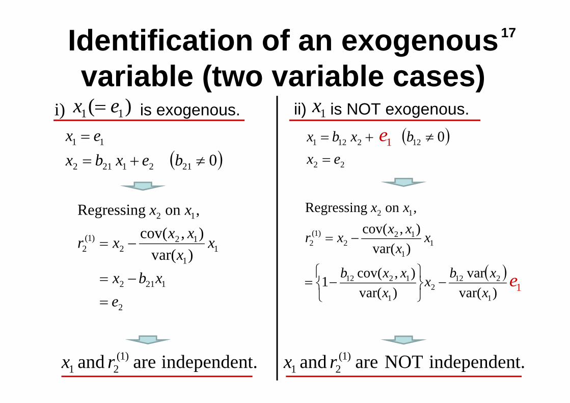
17

( ))var(

var)var(

),cov(1

)var(),cov(,on Regressing

1

2122

1

1212

11

122

)1(2

12

xxbx

xxxb

xx

xxxr

xx

−⎭⎬⎫

⎩⎨⎧−=

−=

2

1212

11

122

)1(2

12

)var(),cov(,on Regressing

exbx

xx

xxxr

xx

=−=

−=

Identification of an exogenous variable (two variable cases)

ii) is NOT exogenous.i) is exogenous.

( )02121212

11

≠+==

bexbxex

)( 11 ex = 1x( )

22

122121 0ex

bxbx=

≠+=

t.independenNOTareand )1(21 rxt.independenareand )1(

21 rx

1e

1e

( )1

1

22

1

1212

11

122

)1(2

21

)var(var

)var(),cov(1

)var(),cov(,on Regressing

ex

xxx

xxb

xx

xxxr

xx

−⎭⎬⎫

⎩⎨⎧−=

−=

( )22

1212121 0ex

bexbx=

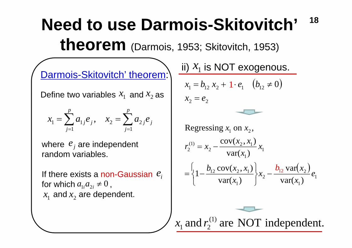
≠⋅+=Darmois-Skitovitch’ theorem:

Define two variables and as

18Need to use Darmois-Skitovitch’ theorem (Darmois, 1953; Skitovitch, 1953)

ii) is NOT exogenous.1x

t.independenNOTareand )1(21 rx

∑∑==

==p

jjj

p

jjj eaxeax

122

111 ,

1x

where are independent random variables.

If there exists a non-Gaussianfor which ,

and are dependent.

je

ie021 ≠iiaa

1x 2x

1

12b

2x

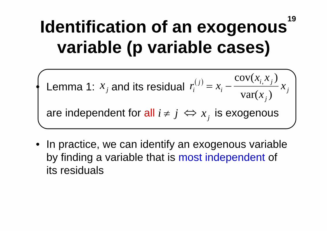
19

• Lemma 1: and its residual

are independent for all is exogenous

• In practice, we can identify an exogenous variable by finding a variable that is most independent of its residuals

Identification of an exogenous variable (p variable cases)

( )j

j

jii

ji x

xxx

xr)var(

)cov( ,−=jx

ji ≠ jx⇔

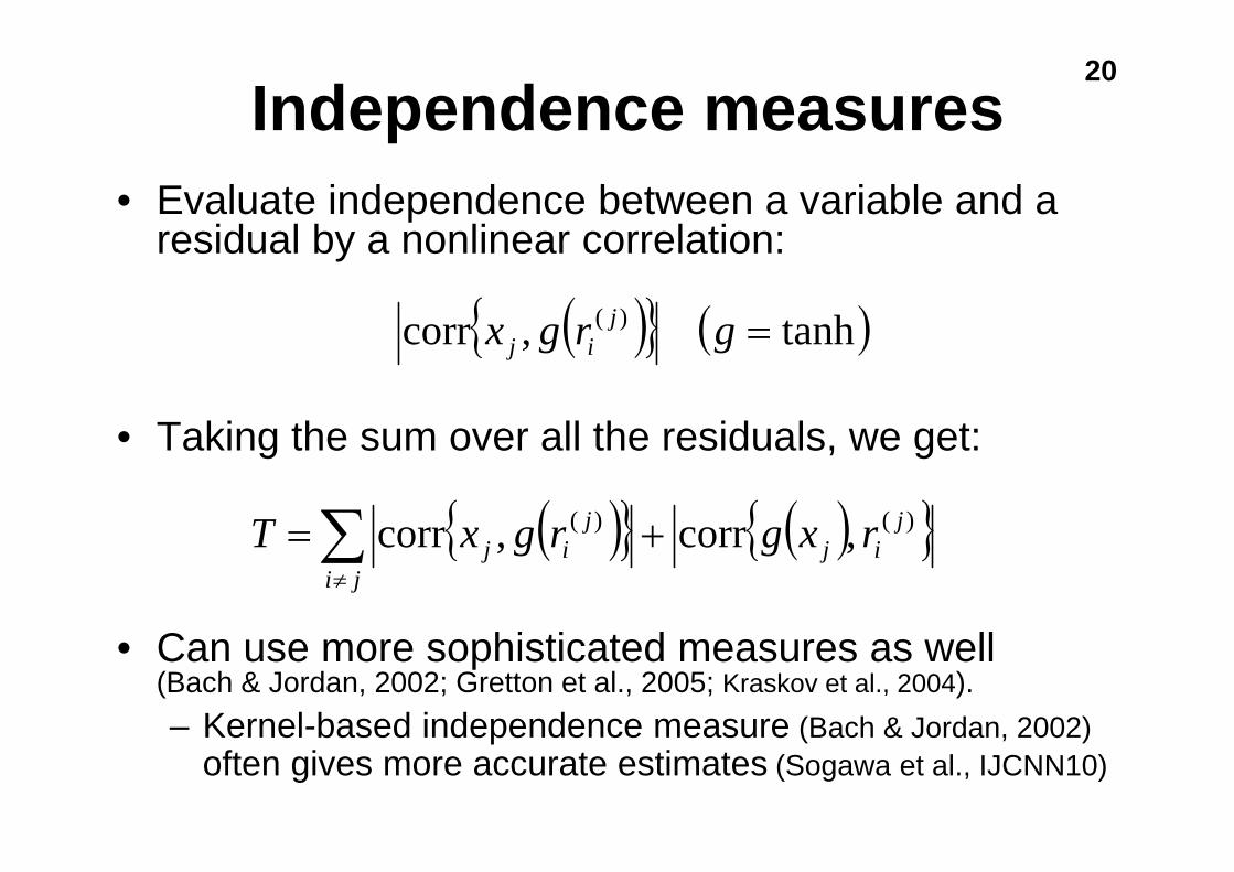
• Evaluate independence between a variable and a residual by a nonlinear correlation:

• Taking the sum over all the residuals, we get:

• Can use more sophisticated measures as well (Bach & Jordan, 2002; Gretton et al., 2005; Kraskov et al., 2004).– Kernel-based independence measure (Bach & Jordan, 2002)

often gives more accurate estimates (Sogawa et al., IJCNN10)

20Independence measures

( ){ } ( )tanh,corr )( =grgx jij

( ){ } ( ){ }∑≠

+=ji

jij

jij rxgrgxT )()( ,corr,corr

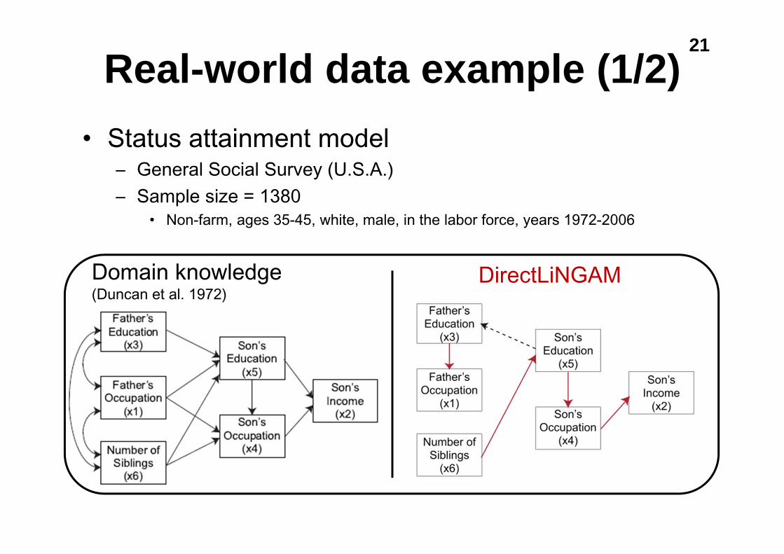
• Status attainment model– General Social Survey (U.S.A.)– Sample size = 1380

• Non-farm, ages 35-45, white, male, in the labor force, years 1972-2006

Domain knowledge (Duncan et al. 1972)

DirectLiNGAM

Real-world data example (1/2)21

Real-world data example (2/2)ICA-LiNGAM

PC algorithm GES

22

23

Summary

• DirectLiNGAM repeats:– Least squares simple linear regression– Evaluation of pairwise independence between each

variable and its residuals

• No algorithmic parameters like stepsize, initial guesses, convergence criteria

• Guaranteed convergence to the right solution in a fixed number of steps (the number of variables) if the data strictly follows the model