ORIGINAL PAPER
Temporal and spatiotemporal autocorrelation of dailyconcentrations of Alnus, Betula, and Corylus pollenin Poland
J. Nowosad • A. Stach • I. Kasprzyk • Ł. Grewling • M. Latałowa •
M. Puc • D. Myszkowska • E. Weryszko- Chmielewska • K. Piotrowska-Weryszko •
K. Chłopek • B. Majkowska-Wojciechowska • A. Uruska
Received: 1 March 2014 / Accepted: 3 November 2014 / Published online: 15 November 2014
� The Author(s) 2014. This article is published with open access at Springerlink.com
Abstract The aim of the study was to determine the
characteristics of temporal and space–time autocorre-
lation of pollen counts of Alnus, Betula, and Corylus in
the air of eight cities in Poland. Daily average pollen
concentrations were monitored over 8 years
(2001–2005 and 2009–2011) using Hirst-designed
volumetric spore traps. The spatial and temporal
coherence of data was investigated using the autocor-
relation and cross-correlation functions. The calcula-
tion and mathematical modelling of 61 correlograms
were performed for up to 25 days back. The study
revealed an association between temporal variations in
Alnus, Betula, and Corylus pollen counts in Poland
and three main groups of factors such as: (1) air mass
exchange after the passage of a single weather front
(30–40 % of pollen count variation); (2) long-lasting
factors (50–60 %); and (3) random factors, including
diurnal variations and measurements errors (10 %).
These results can help to improve the quality of
forecasting models.
J. Nowosad (&) � A. Stach
Institute of Geoecology and Geoinformation, Adam
Mickiewicz University, Dziegielowa 27, 61-680 Poznan,
Poland
e-mail: [email protected]
I. Kasprzyk
Department of Environmental Biology, University of
Rzeszow, Zelwerowicza 4, 35-601 Rzeszow, Poland
Ł. Grewling
Laboratory of Aeropalynology, Faculty of Biology, Adam
Mickiewicz University, Umultowska 89, 61-614 Poznan,
Poland
M. Latałowa � A. Uruska
Department of Plant Ecology, University of Gdansk, Wita
Stwosza 59, 80-308 Gdansk, Poland
M. Puc
Department of Botany and Nature Conservation,
University of Szczecin, Felczaka 3c, 71-412 Szczecin,
Poland
D. Myszkowska
Department of Clinical and Environmental Allergology,
Jagiellonian University Medical College, Sniadeckich 10,
31-531 Krakow, Poland
E. Weryszko- Chmielewska
Department of Botany, University of Life Sciences in
Lublin, Akademicka 15, 20-950 Lublin, Poland
K. Piotrowska-Weryszko
Department of General Ecology, University of Life
Sciences in Lublin, Akademicka 15, 20-950 Lublin,
Poland
K. Chłopek
Faculty of Earth Sciences, University of Silesia,
Bedzinska 60, 41-200 Sosnowiec, Poland
B. Majkowska-Wojciechowska
Department of Immunology, Rheumatology and Allergy,
Faculty of Medicine, Medical University, Pomorska 251,
92-215 Łodz, Poland
123
Aerobiologia (2015) 31:159–177
DOI 10.1007/s10453-014-9354-2
Keywords Tree pollen � Allergenic pollen �Betulaceae � Diurnal variation � Temporal
autocorrelation � Space–time autocorrelation
1 Introduction
Measured at a point, an air pollen count is the result of
many factors affecting the production and dispersion
of pollen in the atmosphere. Hence, changing one or a
few factors usually does not cause an immediate and
abrupt change in pollen concentrations. Rather, the
change is gradual and somewhat delayed. The same
holds for its spatial dimension. Understanding the
character of atmospheric pollen concentrations can
greatly help to improve the quality of forecasting
models. Therefore, it is important in the prophylaxis of
pollen allergies.
Alder (Alnus Mill.), birch (Betula L.), and hazel
(Corylus L.) belong to the order Fagales Engl. and the
family Betulaceae Gray (Bremer et al. 2009). Those
trees are important sources of allergenic pollen in the
temperate climatic zone of the Northern Hemisphere
(Stach et al. 2008). The major pollen allergens from
members of the family Betulaceae are structurally
and immunochemically similar. Therefore, alder,
birch, and hazel allergens have a high degree of
cross-reactivity (Mothes and Valenta 2004). Seasons
with abundant hazel or alder pollen can lead to
stronger reactions to birch pollen and extend the birch
pollen season (Emberlin et al. 1997; Puc 2003;
Rodriguez-Rajo et al. 2004). Approximately 15 % of
the European population suffers from allergies, and
Poland is one of the countries with the highest allergy
incidence rates, up to 45 %. It mostly affects children
and young people (Heinzerling et al. 2009; Pio-
trowska and Kubik-Komar 2012; Malkiewicz et al.
2013). Sensitisation rates to trees belonging to the
family Betulaceae are high in Central/Western
Europe, with Poland showing high sensitisation rates
for alder (22.8 %), birch (27.7 %), and hazel
(22.3 %) (Heinzerling et al. 2009). The number of
pollen grains needed to provoke an allergic reaction
in people depends on individual reactivity and differs
according to species and region. In Poland, the first
allergy symptoms are observed at 20 pollen/m3 of air
for birch, 35 pollen/m3 of air for hazel, and
45 pollen/m3 of air for alder (Rapiejko et al. 2007).
The pollen grain identification is conducted at the
genus level. Each genus has a dominant species in
Poland: Alnus glutinosa, Betula pendula, and less
common Betula pubescens, Corylus avellana, and their
cultivars. All species within a particular genus bloom at
very similar times. Alder and hazel pollen is the first to
appear in the air. The pollination period and the start of
the pollen season are highly variable from year to year
and depend on the rather unstable weather conditions in
late winter and spring (Smith et al. 2007; Kaszewski
et al. 2008; Hajkova et al. 2009; Rodriguez-Rajo et al.
2009; Myszkowska et al. 2011). Alder and hazel shed
their pollen from the end of January to mid-April, while
the birch pollination period is relatively short and
occurs in the second half of April and early May
(Weryszko-Chmielewska et al. 2001; Kluza-Wieloch
and Szewczak 2006; Puc 2007; Grewling et al. 2012a).
Pollination is affected by the geographical location
and local climate. The phases and duration of pollen
seasons as well as the skewness, kurtosis, and annual
totals of pollen grains heavily depend on the geo-
graphical position (Myszkowska et al. 2010). Never-
theless, annual totals of alder and hazel pollen show
different spatial patterns. For Alnus, the annual pollen
total increases from east to west, and for Corylus, there
is an increase in the northerly direction (Myszkowska
et al. 2010). Furthermore, weather conditions such as
mean air temperature, total precipitation, relative
humidity, and wind direction and speed have an
important effect on the duration and intensity of pollen
release and concentration in the air. As a result, these
variables can be used for constructing forecast models
(Rodriguez-Rajo et al. 2009; Puc 2012).
Spatial and space–time autocorrelation is functionally
important in many ecosystems. Pollen production varies
in both space and time; therefore, documenting its
patterns and understanding the causes of variations is
important to aerobiology. Moreover, describing tempo-
ral autocorrelation (one taxon—one location) and space–
time autocorrelation (one taxon—two/many locations)
should be the first step in developing models of pollen
concentrations. Nowadays, autocorrelation analysis is
rarely used in aerobiological research (Rodriguez-Rajo
et al. 2006), except for mast seeding studies. Liebhold
et al. (2003) quantified within-population spatial syn-
chrony in mast dynamics of North American oaks,
Garrison et al. (2006) studied spatial synchrony and
temporal patterns of acorn production in California black
oaks, and Ranta and Satri (2007) analysed the
160 Aerobiologia (2015) 31:159–177
123
synchronisation of high and low pollen years of Betula,
Alnus, Corylus, Salix, and Populus. There has been no
comprehensive analysis of alder, birch, and hazel
temporal and space–time synchrony so far.
The main objective of the present study was to
determine mean multi-year characteristics of temporal
and space–time autocorrelation of the pollen counts of
Alnus, Betula, and Corylus in the air of eight cities in
Poland.
2 Materials and methods
2.1 Study area
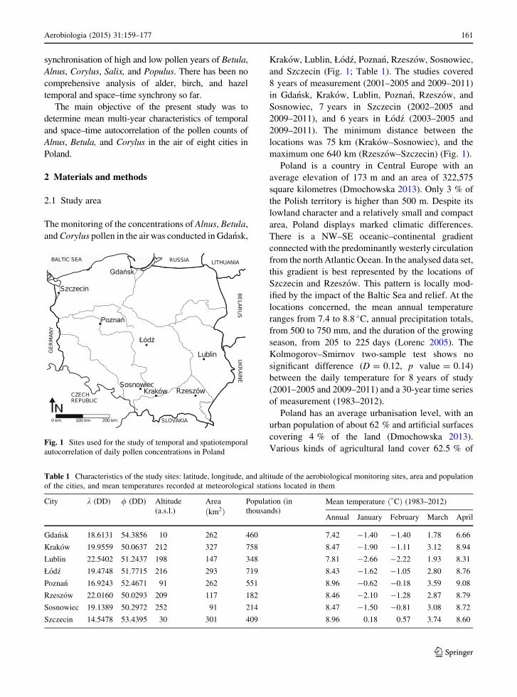
The monitoring of the concentrations of Alnus, Betula,
and Corylus pollen in the air was conducted in Gdansk,
Krakow, Lublin, Łodz, Poznan, Rzeszow, Sosnowiec,
and Szczecin (Fig. 1; Table 1). The studies covered
8 years of measurement (2001–2005 and 2009–2011)
in Gdansk, Krakow, Lublin, Poznan, Rzeszow, and
Sosnowiec, 7 years in Szczecin (2002–2005 and
2009–2011), and 6 years in Łodz (2003–2005 and
2009–2011). The minimum distance between the
locations was 75 km (Krakow–Sosnowiec), and the
maximum one 640 km (Rzeszow–Szczecin) (Fig. 1).
Poland is a country in Central Europe with an
average elevation of 173 m and an area of 322,575
square kilometres (Dmochowska 2013). Only 3 % of
the Polish territory is higher than 500 m. Despite its
lowland character and a relatively small and compact
area, Poland displays marked climatic differences.
There is a NW–SE oceanic–continental gradient
connected with the predominantly westerly circulation
from the north Atlantic Ocean. In the analysed data set,
this gradient is best represented by the locations of
Szczecin and Rzeszow. This pattern is locally mod-
ified by the impact of the Baltic Sea and relief. At the
locations concerned, the mean annual temperature
ranges from 7.4 to 8:8 �C, annual precipitation totals,
from 500 to 750 mm, and the duration of the growing
season, from 205 to 225 days (Lorenc 2005). The
Kolmogorov–Smirnov two-sample test shows no
significant difference (D = 0.12, p value = 0.14)
between the daily temperature for 8 years of study
(2001–2005 and 2009–2011) and a 30-year time series
of measurement (1983–2012).
Poland has an average urbanisation level, with an
urban population of about 62 % and artificial surfaces
covering 4 % of the land (Dmochowska 2013).
Various kinds of agricultural land cover 62.5 % ofFig. 1 Sites used for the study of temporal and spatiotemporal
autocorrelation of daily pollen concentrations in Poland
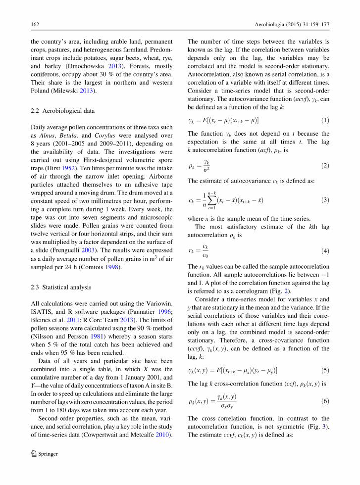
Table 1 Characteristics of the study sites: latitude, longitude, and altitude of the aerobiological monitoring sites, area and population
of the cities, and mean temperatures recorded at meteorological stations located in them
City k (DD) / (DD) Altitude
(a.s.l.)
Area
ðkm2ÞPopulation (in
thousands)Mean temperature ð�CÞ (1983–2012)
Annual January February March April
Gdansk 18.6131 54.3856 10 262 460 7.42 -1.40 -1.40 1.78 6.66
Krakow 19.9559 50.0637 212 327 758 8.47 -1.90 -1.11 3.12 8.94
Lublin 22.5402 51.2437 198 147 348 7.81 -2.66 -2.22 1.93 8.31
Łodz 19.4748 51.7715 216 293 719 8.43 -1.62 -1.05 2.80 8.76
Poznan 16.9243 52.4671 91 262 551 8.96 -0.62 -0.18 3.59 9.08
Rzeszow 22.0160 50.0293 209 117 182 8.46 -2.10 -1.28 2.87 8.79
Sosnowiec 19.1389 50.2972 252 91 214 8.47 -1.50 -0.81 3.08 8.72
Szczecin 14.5478 53.4395 30 301 409 8.96 0.18 0.57 3.74 8.60
Aerobiologia (2015) 31:159–177 161
123
the country’s area, including arable land, permanent
crops, pastures, and heterogeneous farmland. Predom-
inant crops include potatoes, sugar beets, wheat, rye,
and barley (Dmochowska 2013). Forests, mostly
coniferous, occupy about 30 % of the country’s area.
Their share is the largest in northern and western
Poland (Milewski 2013).
2.2 Aerobiological data
Daily average pollen concentrations of three taxa such
as Alnus, Betula, and Corylus were analysed over
8 years (2001–2005 and 2009–2011), depending on
the availability of data. The investigations were
carried out using Hirst-designed volumetric spore
traps (Hirst 1952). Ten litres per minute was the intake
of air through the narrow inlet opening. Airborne
particles attached themselves to an adhesive tape
wrapped around a moving drum. The drum moved at a
constant speed of two millimetres per hour, perform-
ing a complete turn during 1 week. Every week, the
tape was cut into seven segments and microscopic
slides were made. Pollen grains were counted from
twelve vertical or four horizontal strips, and their sum
was multiplied by a factor dependent on the surface of
a slide (Frenguelli 2003). The results were expressed
as a daily average number of pollen grains in m3 of air
sampled per 24 h (Comtois 1998).
2.3 Statistical analysis
All calculations were carried out using the Variowin,
ISATIS, and R software packages (Pannatier 1996;
Bleines et al. 2011; R Core Team 2013). The limits of
pollen seasons were calculated using the 90 % method
(Nilsson and Persson 1981) whereby a season starts
when 5 % of the total catch has been achieved and
ends when 95 % has been reached.
Data of all years and particular site have been
combined into a single table, in which X was the
cumulative number of a day from 1 January 2001, and
Y—the value of daily concentrations of taxon A in site B.
In order to speed up calculations and eliminate the large
number of lagswith zero concentration values, the period
from 1 to 180 days was taken into account each year.
Second-order properties, such as the mean, vari-
ance, and serial correlation, play a key role in the study
of time-series data (Cowpertwait and Metcalfe 2010).
The number of time steps between the variables is
known as the lag. If the correlation between variables
depends only on the lag, the variables may be
correlated and the model is second-order stationary.
Autocorrelation, also known as serial correlation, is a
correlation of a variable with itself at different times.
Consider a time-series model that is second-order
stationary. The autocovariance function (acvf), ck, can
be defined as a function of the lag k:
ck ¼ E½ðxt � lÞðxtþk � lÞ� ð1Þ
The function ck does not depend on t because the
expectation is the same at all times t. The lag
k autocorrelation function (acf), qk, is
qk ¼ck
r2ð2Þ
The estimate of autocovariance ck is defined as:
ck ¼1
n
Xn�k
t¼1
ðxt � �xÞðxtþk � �xÞ ð3Þ
where �x is the sample mean of the time series.
The most satisfactory estimate of the kth lag
autocorrelation qk is
rk ¼ck
c0ð4Þ
The rk values can be called the sample autocorrelation
function. All sample autocorrelations lie between �1
and 1. A plot of the correlation function against the lag
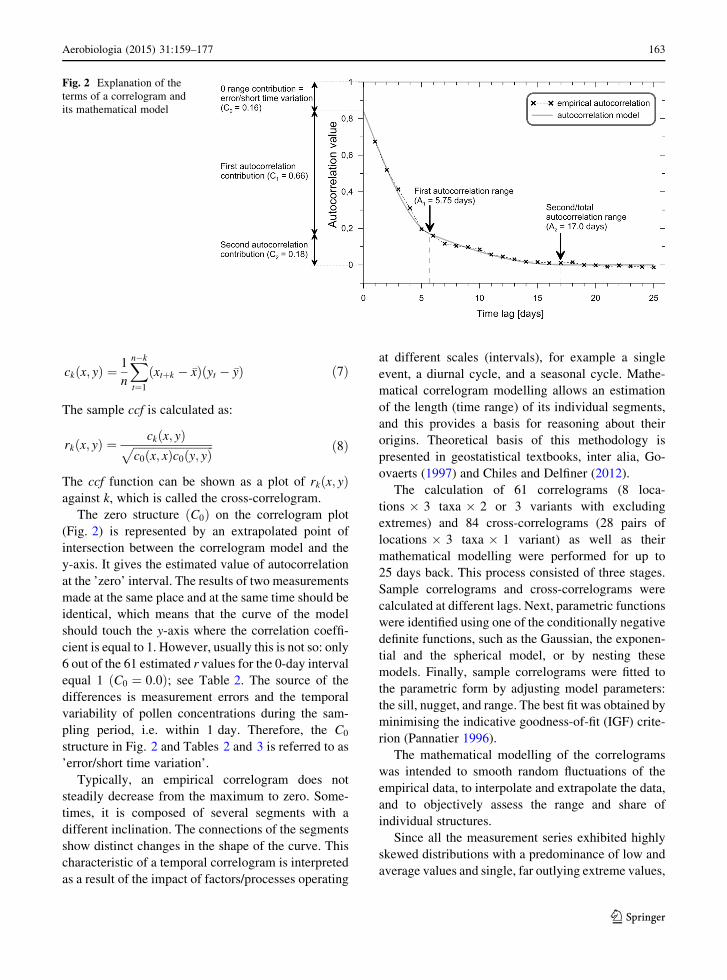
is referred to as a correlogram (Fig. 2).
Consider a time-series model for variables x and
y that are stationary in the mean and the variance. If the
serial correlations of those variables and their corre-
lations with each other at different time lags depend
only on a lag, the combined model is second-order
stationary. Therefore, a cross-covariance function
(ccvf), ckðx; yÞ, can be defined as a function of the
lag, k:
ckðx; yÞ ¼ E½ðxtþk � lxÞðyt � lyÞ� ð5Þ
The lag k cross-correlation function (ccf), qkðx; yÞ is
qkðx; yÞ ¼ ckðx; yÞrxry
ð6Þ
The cross-correlation function, in contrast to the
autocorrelation function, is not symmetric (Fig. 3).
The estimate ccvf, ckðx; yÞ is defined as:
162 Aerobiologia (2015) 31:159–177
123
ckðx; yÞ ¼ 1
n
Xn�k
t¼1
ðxtþk � �xÞðyt � �yÞ ð7Þ
The sample ccf is calculated as:
rkðx; yÞ ¼ ckðx; yÞffiffiffiffiffiffiffiffiffiffiffiffiffiffiffiffiffiffiffiffiffiffiffiffiffiffiffiffiffic0ðx; xÞc0ðy; yÞ
p ð8Þ
The ccf function can be shown as a plot of rkðx; yÞagainst k, which is called the cross-correlogram.
The zero structure ðC0Þ on the correlogram plot
(Fig. 2) is represented by an extrapolated point of
intersection between the correlogram model and the
y-axis. It gives the estimated value of autocorrelation
at the ’zero’ interval. The results of two measurements
made at the same place and at the same time should be
identical, which means that the curve of the model
should touch the y-axis where the correlation coeffi-
cient is equal to 1. However, usually this is not so: only
6 out of the 61 estimated r values for the 0-day interval
equal 1 ðC0 ¼ 0:0Þ; see Table 2. The source of the
differences is measurement errors and the temporal
variability of pollen concentrations during the sam-
pling period, i.e. within 1 day. Therefore, the C0
structure in Fig. 2 and Tables 2 and 3 is referred to as
’error/short time variation’.
Typically, an empirical correlogram does not
steadily decrease from the maximum to zero. Some-
times, it is composed of several segments with a
different inclination. The connections of the segments
show distinct changes in the shape of the curve. This
characteristic of a temporal correlogram is interpreted
as a result of the impact of factors/processes operating
at different scales (intervals), for example a single
event, a diurnal cycle, and a seasonal cycle. Mathe-
matical correlogram modelling allows an estimation
of the length (time range) of its individual segments,
and this provides a basis for reasoning about their
origins. Theoretical basis of this methodology is
presented in geostatistical textbooks, inter alia, Go-
ovaerts (1997) and Chiles and Delfiner (2012).
The calculation of 61 correlograms (8 loca-
tions � 3 taxa � 2 or 3 variants with excluding
extremes) and 84 cross-correlograms (28 pairs of
locations � 3 taxa � 1 variant) as well as their
mathematical modelling were performed for up to
25 days back. This process consisted of three stages.
Sample correlograms and cross-correlograms were
calculated at different lags. Next, parametric functions
were identified using one of the conditionally negative
definite functions, such as the Gaussian, the exponen-
tial and the spherical model, or by nesting these
models. Finally, sample correlograms were fitted to
the parametric form by adjusting model parameters:
the sill, nugget, and range. The best fit was obtained by
minimising the indicative goodness-of-fit (IGF) crite-
rion (Pannatier 1996).
The mathematical modelling of the correlograms
was intended to smooth random fluctuations of the
empirical data, to interpolate and extrapolate the data,
and to objectively assess the range and share of
individual structures.
Since all the measurement series exhibited highly
skewed distributions with a predominance of low and
average values and single, far outlying extreme values,
Fig. 2 Explanation of the
terms of a correlogram and
its mathematical model
Aerobiologia (2015) 31:159–177 163
123
the autocorrelation analysis was conducted twice: for
the entire set and with the extremes eliminated. For the
determination of extreme values, two threshold values
were used. The first was put at the place of disruption
of the frequency histogram (selection 1), the other cut
off the data outliers (selection 2) (Fig. 5).
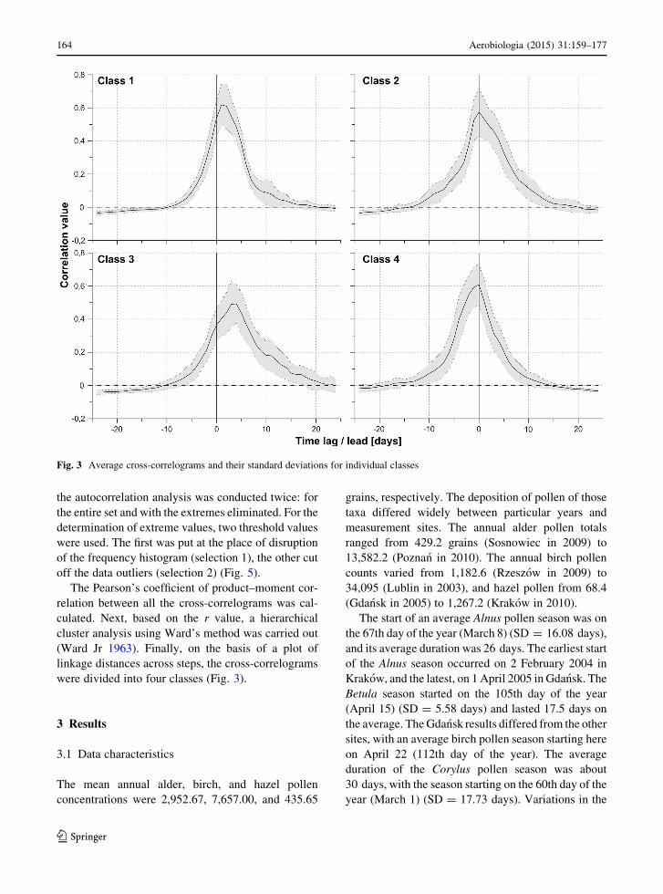
The Pearson’s coefficient of product–moment cor-
relation between all the cross-correlograms was cal-
culated. Next, based on the r value, a hierarchical
cluster analysis using Ward’s method was carried out
(Ward Jr 1963). Finally, on the basis of a plot of
linkage distances across steps, the cross-correlograms
were divided into four classes (Fig. 3).
3 Results
3.1 Data characteristics
The mean annual alder, birch, and hazel pollen
concentrations were 2,952.67, 7,657.00, and 435.65
grains, respectively. The deposition of pollen of those
taxa differed widely between particular years and
measurement sites. The annual alder pollen totals
ranged from 429.2 grains (Sosnowiec in 2009) to
13,582.2 (Poznan in 2010). The annual birch pollen
counts varied from 1,182.6 (Rzeszow in 2009) to
34,095 (Lublin in 2003), and hazel pollen from 68.4
(Gdansk in 2005) to 1,267.2 (Krakow in 2010).
The start of an average Alnus pollen season was on
the 67th day of the year (March 8) (SD = 16.08 days),
and its average duration was 26 days. The earliest start
of the Alnus season occurred on 2 February 2004 in
Krakow, and the latest, on 1 April 2005 in Gdansk. The
Betula season started on the 105th day of the year
(April 15) (SD = 5.58 days) and lasted 17.5 days on
the average. The Gdansk results differed from the other
sites, with an average birch pollen season starting here
on April 22 (112th day of the year). The average
duration of the Corylus pollen season was about
30 days, with the season starting on the 60th day of the
year (March 1) (SD = 17.73 days). Variations in the
Fig. 3 Average cross-correlograms and their standard deviations for individual classes
164 Aerobiologia (2015) 31:159–177
123
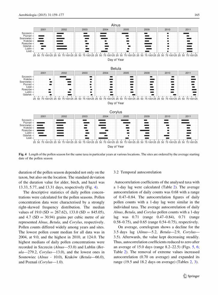
duration of the pollen season depended not only on the
taxon, but also on the location. The standard deviation
of the duration value for alder, birch, and hazel was
13.33, 5.77, and 13.31 days, respectively (Fig. 4).
The descriptive statistics of daily pollen concen-
trations were calculated for the pollen seasons. Pollen
concentration data were characterised by a strongly
right-skewed frequency distribution. The median
values of 19.0 (SD = 267.62), 133.0 (SD = 845.05),
and 4.7 (SD = 30.94) grains per cubic metre of air
represented Alnus, Betula, and Corylus, respectively.
Pollen counts differed widely among years and sites.
The lowest pollen count median for all data was in
2004, at 9.0, and the highest in 2010, at 124.0. The
highest medians of daily pollen concentrations were
recorded in Szczecin (Alnus—53.0) and Lublin (Bet-
ula—279.2, Corylus—13.0), and the lowest ones in
Sosnowiec (Alnus - 10.0), Krakow (Betula—66.0),
and Poznan (Corylus—1.0).
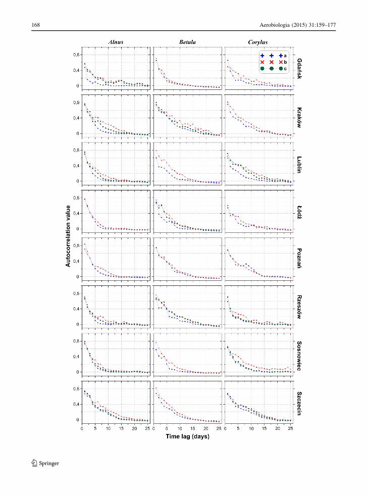
3.2 Temporal autocorrelation
Autocorrelation coefficients of the analysed taxa with
a 1-day lag were calculated (Table 2). The average
autocorrelation of daily counts was 0.68 with a range
of 0.47–0.84. The autocorrelation figures of daily
pollen counts with a 1-day lag were similar in the
individual taxa. The average autocorrelation of daily
Alnus, Betula, and Corylus pollen counts with a 1-day
lag was 0.71 (range 0.47–0.84), 0.71 (range
0.58–0.75), and 0.65 (range 0.54–0.75), respectively.
On average, correlogram shows a decline for the
3.5 days lag (Alnus—5.2, Betula—2.9, Corylus—
3.5). Afterwards, the value kept decreasing steadily.
Thus, autocorrelation coefficients reduced to zero after
an average of 15.0 days (range 8.2–22.5) (Figs. 5, 6;
Table 2). The removal of extreme values increased
autocorrelation (0.70 on average) and expanded its
range (19.5 and 18.2 days on average) (Tables 2, 3).
Fig. 4 Length of the pollen season for the same taxa in particular years at various locations. The sites are ordered by the average starting
date of the pollen season
Aerobiologia (2015) 31:159–177 165
123
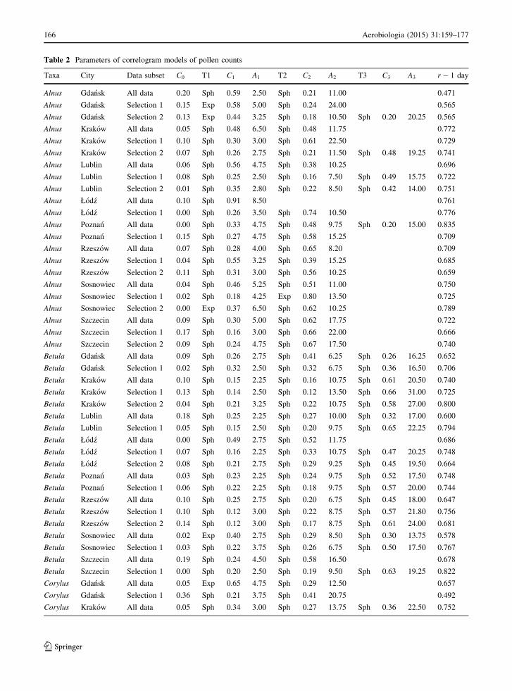
Table 2 Parameters of correlogram models of pollen counts
Taxa City Data subset C0 T1 C1 A1 T2 C2 A2 T3 C3 A3 r � 1 day
Alnus Gdansk All data 0.20 Sph 0.59 2.50 Sph 0.21 11.00 0.471
Alnus Gdansk Selection 1 0.15 Exp 0.58 5.00 Sph 0.24 24.00 0.565
Alnus Gdansk Selection 2 0.13 Exp 0.44 3.25 Sph 0.18 10.50 Sph 0.20 20.25 0.565
Alnus Krakow All data 0.05 Sph 0.48 6.50 Sph 0.48 11.75 0.772
Alnus Krakow Selection 1 0.10 Sph 0.30 3.00 Sph 0.61 22.50 0.729
Alnus Krakow Selection 2 0.07 Sph 0.26 2.75 Sph 0.21 11.50 Sph 0.48 19.25 0.741
Alnus Lublin All data 0.06 Sph 0.56 4.75 Sph 0.38 10.25 0.696
Alnus Lublin Selection 1 0.08 Sph 0.25 2.50 Sph 0.16 7.50 Sph 0.49 15.75 0.722
Alnus Lublin Selection 2 0.01 Sph 0.35 2.80 Sph 0.22 8.50 Sph 0.42 14.00 0.751
Alnus Łodz All data 0.10 Sph 0.91 8.50 0.761
Alnus Łodz Selection 1 0.00 Sph 0.26 3.50 Sph 0.74 10.50 0.776
Alnus Poznan All data 0.00 Sph 0.33 4.75 Sph 0.48 9.75 Sph 0.20 15.00 0.835
Alnus Poznan Selection 1 0.15 Sph 0.27 4.75 Sph 0.58 15.25 0.709
Alnus Rzeszow All data 0.07 Sph 0.28 4.00 Sph 0.65 8.20 0.709
Alnus Rzeszow Selection 1 0.04 Sph 0.55 3.25 Sph 0.39 15.25 0.685
Alnus Rzeszow Selection 2 0.11 Sph 0.31 3.00 Sph 0.56 10.25 0.659
Alnus Sosnowiec All data 0.04 Sph 0.46 5.25 Sph 0.51 11.00 0.750
Alnus Sosnowiec Selection 1 0.02 Sph 0.18 4.25 Exp 0.80 13.50 0.725
Alnus Sosnowiec Selection 2 0.00 Exp 0.37 6.50 Sph 0.62 10.25 0.789
Alnus Szczecin All data 0.09 Sph 0.30 5.00 Sph 0.62 17.75 0.722
Alnus Szczecin Selection 1 0.17 Sph 0.16 3.00 Sph 0.66 22.00 0.666
Alnus Szczecin Selection 2 0.09 Sph 0.24 4.75 Sph 0.67 17.50 0.740
Betula Gdansk All data 0.09 Sph 0.26 2.75 Sph 0.41 6.25 Sph 0.26 16.25 0.652
Betula Gdansk Selection 1 0.02 Sph 0.32 2.50 Sph 0.32 6.75 Sph 0.36 16.50 0.706
Betula Krakow All data 0.10 Sph 0.15 2.25 Sph 0.16 10.75 Sph 0.61 20.50 0.740
Betula Krakow Selection 1 0.13 Sph 0.14 2.50 Sph 0.12 13.50 Sph 0.66 31.00 0.725
Betula Krakow Selection 2 0.04 Sph 0.21 3.25 Sph 0.22 10.75 Sph 0.58 27.00 0.800
Betula Lublin All data 0.18 Sph 0.25 2.25 Sph 0.27 10.00 Sph 0.32 17.00 0.600
Betula Lublin Selection 1 0.05 Sph 0.15 2.50 Sph 0.20 9.75 Sph 0.65 22.25 0.794
Betula Łodz All data 0.00 Sph 0.49 2.75 Sph 0.52 11.75 0.686
Betula Łodz Selection 1 0.07 Sph 0.16 2.25 Sph 0.33 10.75 Sph 0.47 20.25 0.748
Betula Łodz Selection 2 0.08 Sph 0.21 2.75 Sph 0.29 9.25 Sph 0.45 19.50 0.664
Betula Poznan All data 0.03 Sph 0.23 2.25 Sph 0.24 9.75 Sph 0.52 17.50 0.748
Betula Poznan Selection 1 0.06 Sph 0.22 2.25 Sph 0.18 9.75 Sph 0.57 20.00 0.744
Betula Rzeszow All data 0.10 Sph 0.25 2.75 Sph 0.20 6.75 Sph 0.45 18.00 0.647
Betula Rzeszow Selection 1 0.10 Sph 0.12 3.00 Sph 0.22 8.75 Sph 0.57 21.80 0.756
Betula Rzeszow Selection 2 0.14 Sph 0.12 3.00 Sph 0.17 8.75 Sph 0.61 24.00 0.681
Betula Sosnowiec All data 0.02 Exp 0.40 2.75 Sph 0.29 8.50 Sph 0.30 13.75 0.578
Betula Sosnowiec Selection 1 0.03 Sph 0.22 3.75 Sph 0.26 6.75 Sph 0.50 17.50 0.767
Betula Szczecin All data 0.19 Sph 0.24 4.50 Sph 0.58 16.50 0.678
Betula Szczecin Selection 1 0.00 Sph 0.20 2.50 Sph 0.19 9.50 Sph 0.63 19.25 0.822
Corylus Gdansk All data 0.05 Exp 0.65 4.75 Sph 0.29 12.50 0.657
Corylus Gdansk Selection 1 0.36 Sph 0.21 3.75 Sph 0.41 20.75 0.492
Corylus Krakow All data 0.05 Sph 0.34 3.00 Sph 0.27 13.75 Sph 0.36 22.50 0.752
166 Aerobiologia (2015) 31:159–177
123
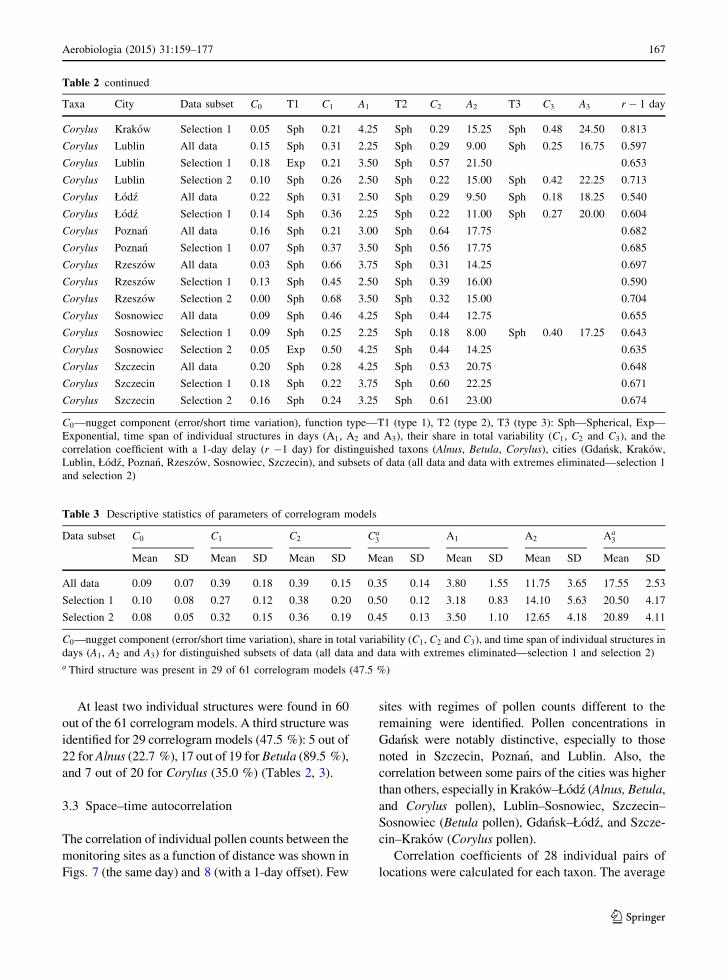
At least two individual structures were found in 60
out of the 61 correlogram models. A third structure was
identified for 29 correlogram models (47.5 %): 5 out of
22 for Alnus (22.7 %), 17 out of 19 for Betula (89.5 %),
and 7 out of 20 for Corylus (35.0 %) (Tables 2, 3).
3.3 Space–time autocorrelation
The correlation of individual pollen counts between the
monitoring sites as a function of distance was shown in
Figs. 7 (the same day) and 8 (with a 1-day offset). Few
sites with regimes of pollen counts different to the
remaining were identified. Pollen concentrations in
Gdansk were notably distinctive, especially to those
noted in Szczecin, Poznan, and Lublin. Also, the
correlation between some pairs of the cities was higher
than others, especially in Krakow–Łodz (Alnus, Betula,
and Corylus pollen), Lublin–Sosnowiec, Szczecin–
Sosnowiec (Betula pollen), Gdansk–Łodz, and Szcze-
cin–Krakow (Corylus pollen).
Correlation coefficients of 28 individual pairs of
locations were calculated for each taxon. The average
Table 2 continued
Taxa City Data subset C0 T1 C1 A1 T2 C2 A2 T3 C3 A3 r � 1 day
Corylus Krakow Selection 1 0.05 Sph 0.21 4.25 Sph 0.29 15.25 Sph 0.48 24.50 0.813
Corylus Lublin All data 0.15 Sph 0.31 2.25 Sph 0.29 9.00 Sph 0.25 16.75 0.597
Corylus Lublin Selection 1 0.18 Exp 0.21 3.50 Sph 0.57 21.50 0.653
Corylus Lublin Selection 2 0.10 Sph 0.26 2.50 Sph 0.22 15.00 Sph 0.42 22.25 0.713
Corylus Łodz All data 0.22 Sph 0.31 2.50 Sph 0.29 9.50 Sph 0.18 18.25 0.540
Corylus Łodz Selection 1 0.14 Sph 0.36 2.25 Sph 0.22 11.00 Sph 0.27 20.00 0.604
Corylus Poznan All data 0.16 Sph 0.21 3.00 Sph 0.64 17.75 0.682
Corylus Poznan Selection 1 0.07 Sph 0.37 3.50 Sph 0.56 17.75 0.685
Corylus Rzeszow All data 0.03 Sph 0.66 3.75 Sph 0.31 14.25 0.697
Corylus Rzeszow Selection 1 0.13 Sph 0.45 2.50 Sph 0.39 16.00 0.590
Corylus Rzeszow Selection 2 0.00 Sph 0.68 3.50 Sph 0.32 15.00 0.704
Corylus Sosnowiec All data 0.09 Sph 0.46 4.25 Sph 0.44 12.75 0.655
Corylus Sosnowiec Selection 1 0.09 Sph 0.25 2.25 Sph 0.18 8.00 Sph 0.40 17.25 0.643
Corylus Sosnowiec Selection 2 0.05 Exp 0.50 4.25 Sph 0.44 14.25 0.635
Corylus Szczecin All data 0.20 Sph 0.28 4.25 Sph 0.53 20.75 0.648
Corylus Szczecin Selection 1 0.18 Sph 0.22 3.75 Sph 0.60 22.25 0.671
Corylus Szczecin Selection 2 0.16 Sph 0.24 3.25 Sph 0.61 23.00 0.674
C0—nugget component (error/short time variation), function type—T1 (type 1), T2 (type 2), T3 (type 3): Sph—Spherical, Exp—
Exponential, time span of individual structures in days (A1, A2 and A3), their share in total variability (C1, C2 and C3), and the
correlation coefficient with a 1-day delay (r �1 day) for distinguished taxons (Alnus, Betula, Corylus), cities (Gdansk, Krakow,
Lublin, Łodz, Poznan, Rzeszow, Sosnowiec, Szczecin), and subsets of data (all data and data with extremes eliminated—selection 1
and selection 2)
Table 3 Descriptive statistics of parameters of correlogram models
Data subset C0 C1 C2 Ca3 A1 A2 Aa
3
Mean SD Mean SD Mean SD Mean SD Mean SD Mean SD Mean SD
All data 0.09 0.07 0.39 0.18 0.39 0.15 0.35 0.14 3.80 1.55 11.75 3.65 17.55 2.53
Selection 1 0.10 0.08 0.27 0.12 0.38 0.20 0.50 0.12 3.18 0.83 14.10 5.63 20.50 4.17
Selection 2 0.08 0.05 0.32 0.15 0.36 0.19 0.45 0.13 3.50 1.10 12.65 4.18 20.89 4.11
C0—nugget component (error/short time variation), share in total variability (C1, C2 and C3), and time span of individual structures in
days (A1, A2 and A3) for distinguished subsets of data (all data and data with extremes eliminated—selection 1 and selection 2)a Third structure was present in 29 of 61 correlogram models (47.5 %)
Aerobiologia (2015) 31:159–177 167
123
168 Aerobiologia (2015) 31:159–177
123
value was 0.58 (range 0.20–0.89). Correlation coeffi-
cients varied from 0.566 to 0.583. Furthermore, they
were clearly, though not very strongly, dependent on
the distance between pairs of monitoring sites (Fig. 7).
With a 1-day lag, the correlation coefficients dropped
to 0.49 (range 0.15–0.70) but the impact of distance
still existed. The Kolmogorov–Smirnov two-sample
test showed no significant differences between corre-
lation coefficients of pairs of the observed taxa
(Alnus–Betula, Alnus–Corylus, and Betula–Corylus).
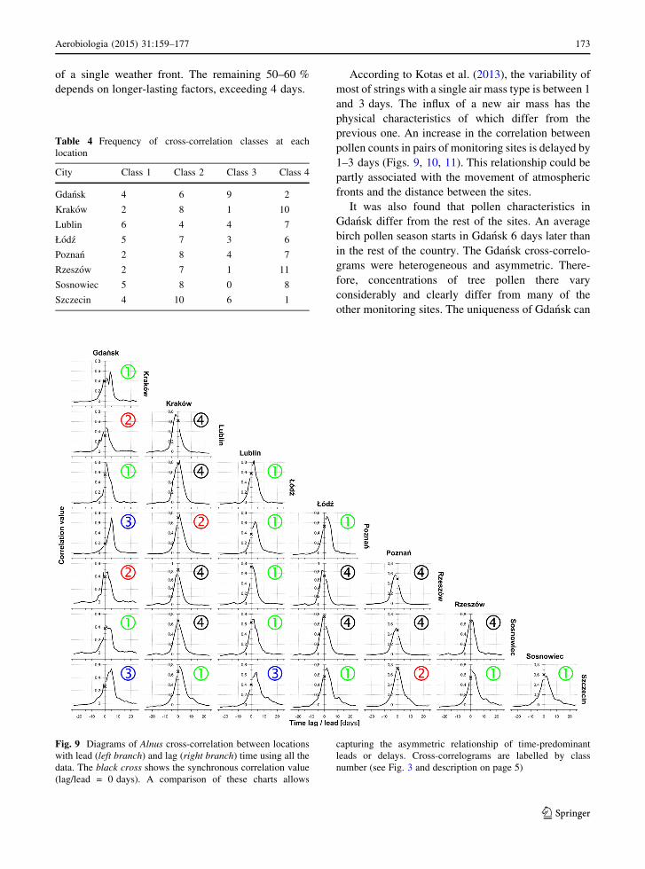
Figures 9, 10, 11 show cross-correlograms of Al-
nus, Betula, and Corylus pollen counts in Poland.
Cross-correlograms of alder were the most homoge-
neous, with symmetric and simple shapes. Moreover,
the temporal range of pollen counts was the shortest, in
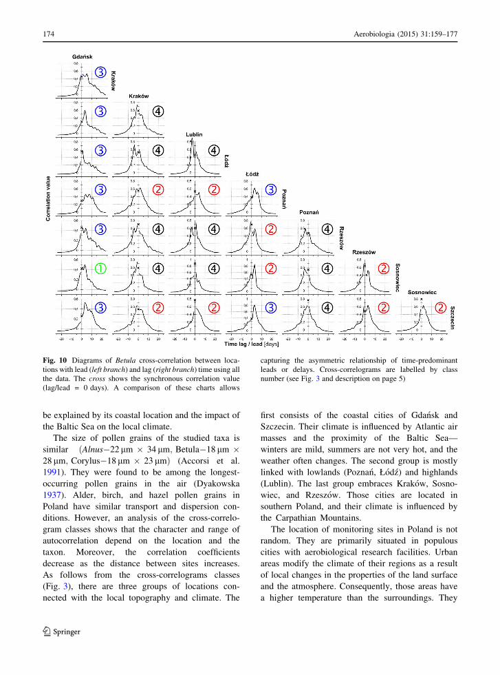
most cases it did not exceed 10 days. Most of birch
and hazel cross-correlograms had an asymmetrical
shape, often with a few oscillations. Its range was
generally longer, sometimes even more than 20 days.
Furthermore, correlation rose along with a 1- to 5-day
lag/lead in numerous pairs of monitoring sites. The
strongest variation was seen in the case of Gdansk.
Most of its cross-correlograms were asymmetric and
showed considerable variation.
The average cross-correlograms and their standard
deviations for individual classes was shown in Fig. 3.
In classes 2 and 4, the maximum correlation occurs on
the same day (zero lag). They differ in a rate of
correlation decrease in the direction of leads and
delays. Their shapes are almost a reflection symmetry.
Class 1 has a symmetric shape with a maximum
delayed by 1 day. Class 3 has the lowest maximum
correlation (0.5), the largest shift (lag of 4–5 days),
and the most asymmetric shape.
The Chi-square test was used to examine whether
the cross-correlogram classes (Fig. 3) depended on the
taxon or the location. It showed a statistically signif-
icant relationship between the classes and the taxa
(p value ’ 0:0002), and between the classes and the
location (p value ’ 0:01). The first class was mostly
Alnus (80 % of the class), the second class—Corylus
(55 %), and the third class—Betula (57 %). Only in
the fourth class, no taxa were dominating. However,
the fourth class differentiates between the locations.
This class occurred mostly in Krakow (10 out of 52)
and Rzeszow (11 out of 52), and very rarely in Gdansk
(2 out of 52) and Szczecin (1 out of 52). In the third
class, differentiation between the locations also
occurred, with zero or a few cases in Sosnowiec (0
out of 28), Krakow (1 out of 28), and Rzeszow (1 out
of 28) (Table 4).
The locations were classified by the frequency of
the occurrence of the cross-correlogram class (Figs.
3, 9, 10, 11). There were major similarities between
Krakow and Rzeszow, and Lublin and Łodz. Three
groups were distinguished, the first consisting of
Krakow, Rzeszow, and Sosnowiec; the second of
Lublin, Łodz, and Poznan; and the third of Gdansk and
Szczecin.
4 Discussion
Local and regional flora and land-use substantially
affect the pollen spectrum. However, pollen concen-
trations in the air depend on more factors, including
the vegetation structure, ability of particular taxa to
spread their pollen, and the topoclimate and weather
conditions in the current and preceding years. Espe-
cially, the effect of temperature on the intensity of the
pollen season is often stressed (Corden et al. 2002;
Rasmussen 2002).
Most pollen studies have focused on changes
through time; hence, patterns across space remain
largely unknown (Grewling et al. 2012b; Leon Ruiz
et al. 2012; Ziello et al. 2012). Little research has been
devoted to a spatial analysis of tree pollen in Poland.
Myszkowska et al. (2010) investigated the relationship
between the geographical location and the dynamics
of Alnus and Corylus pollen seasons in Poland.
However, temporal and spatiotemporal autocorrela-
tion has not been taken into account before.
The form of the correlograms provides an under-
standing of the temporal variations in Alnus, Betula,
and Corylus pollen counts in Poland. Notable changes
in the shapes of the correlograms suggest that varia-
tions may be associated with three main groups of
factors. 10 % of pollen count variations can be due to
random factors, including diurnal fluctuations and
measurement errors (Tables 2, 3). The autocorrelation
value dropped substantially after 3.5 days. Thus,
approximately 30–40 % of the variation could be
caused by an exchange of air masses after the passage
bFig. 5 Matrix of sample (experimental) correlogram plots for
the entire data set (a) and after the elimination of extreme figures
(b-first threshold, c-second threshold) for the individual
locations (rows) and taxa (columns)
Aerobiologia (2015) 31:159–177 169
123
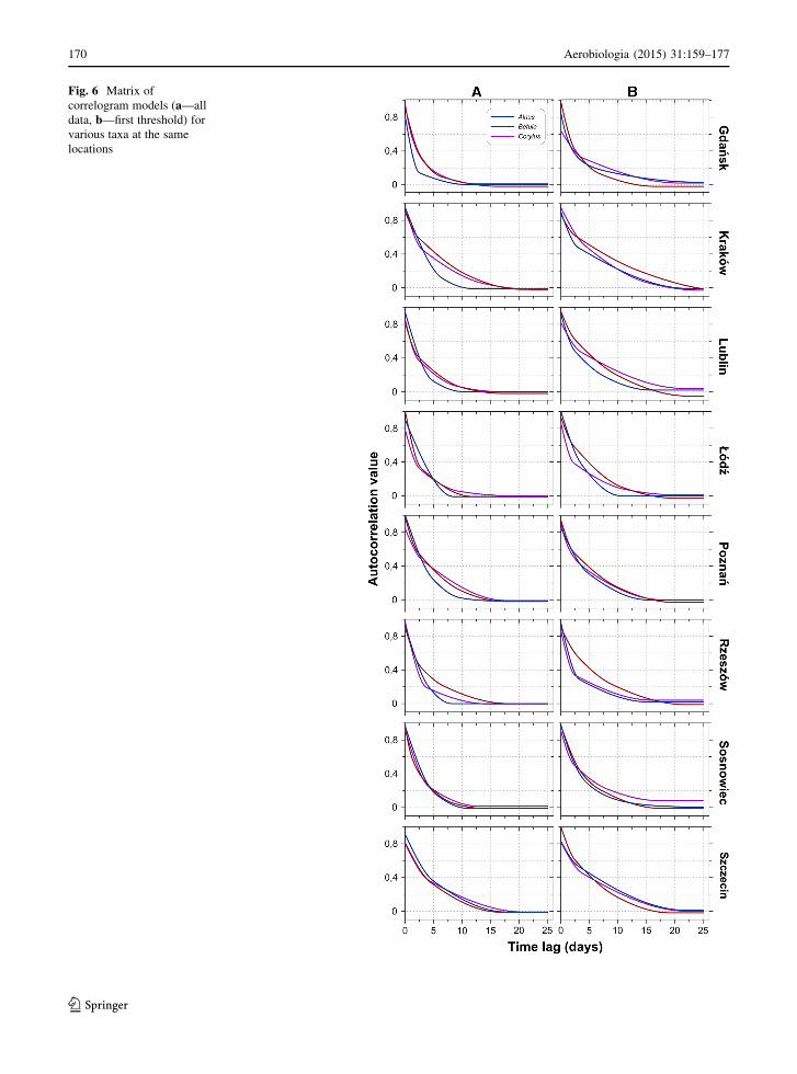
Fig. 6 Matrix of
correlogram models (a—all
data, b—first threshold) for
various taxa at the same
locations
170 Aerobiologia (2015) 31:159–177
123
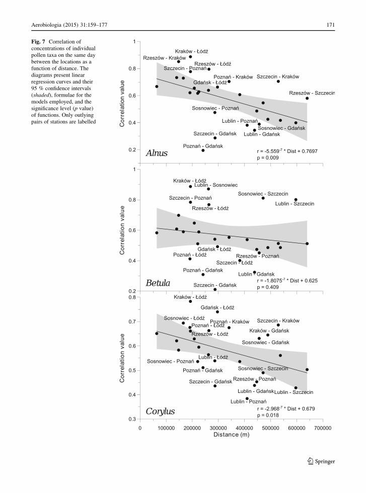
Fig. 7 Correlation of
concentrations of individual
pollen taxa on the same day
between the locations as a
function of distance. The
diagrams present linear
regression curves and their
95 % confidence intervals
(shaded), formulae for the
models employed, and the
significance level (p value)
of functions. Only outlying
pairs of stations are labelled
Aerobiologia (2015) 31:159–177 171
123
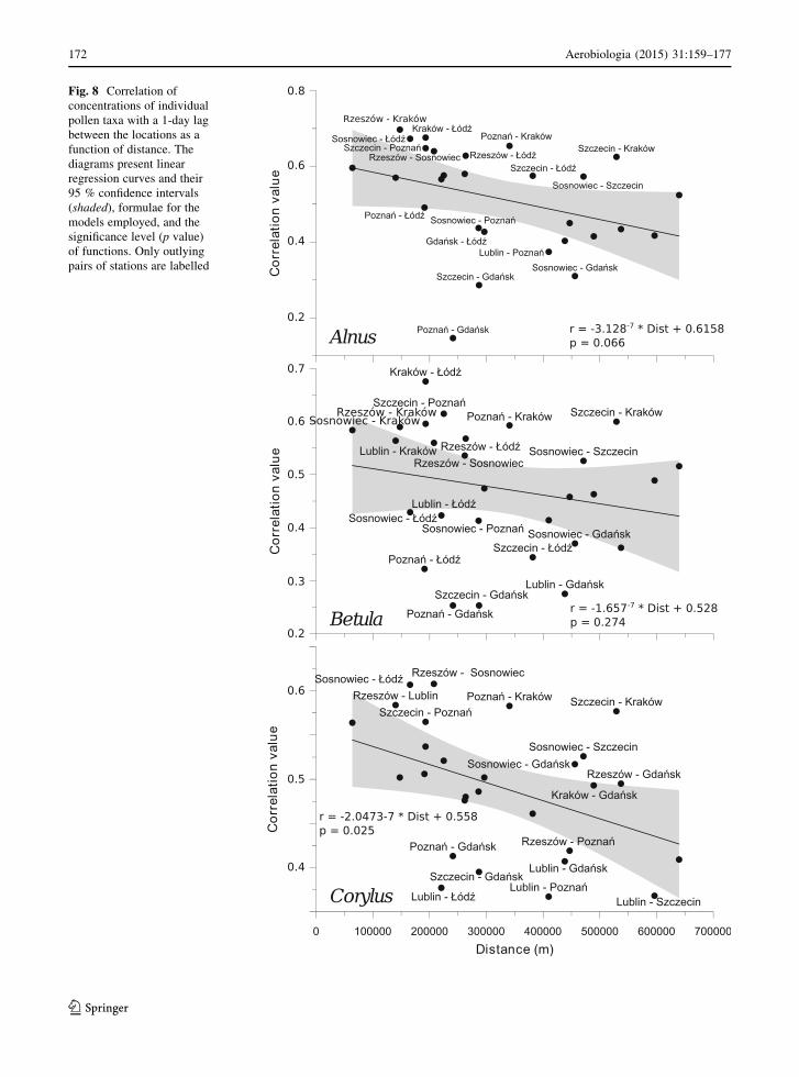
Fig. 8 Correlation of
concentrations of individual
pollen taxa with a 1-day lag
between the locations as a
function of distance. The
diagrams present linear
regression curves and their
95 % confidence intervals
(shaded), formulae for the
models employed, and the
significance level (p value)
of functions. Only outlying
pairs of stations are labelled
172 Aerobiologia (2015) 31:159–177
123
of a single weather front. The remaining 50–60 %
depends on longer-lasting factors, exceeding 4 days.
According to Kotas et al. (2013), the variability of
most of strings with a single air mass type is between 1
and 3 days. The influx of a new air mass has the
physical characteristics of which differ from the
previous one. An increase in the correlation between
pollen counts in pairs of monitoring sites is delayed by
1–3 days (Figs. 9, 10, 11). This relationship could be
partly associated with the movement of atmospheric
fronts and the distance between the sites.
It was also found that pollen characteristics in
Gdansk differ from the rest of the sites. An average
birch pollen season starts in Gdansk 6 days later than
in the rest of the country. The Gdansk cross-correlo-
grams were heterogeneous and asymmetric. There-
fore, concentrations of tree pollen there vary
considerably and clearly differ from many of the
other monitoring sites. The uniqueness of Gdansk can
Fig. 9 Diagrams of Alnus cross-correlation between locations
with lead (left branch) and lag (right branch) time using all the
data. The black cross shows the synchronous correlation value
(lag/lead = 0 days). A comparison of these charts allows
capturing the asymmetric relationship of time-predominant
leads or delays. Cross-correlograms are labelled by class
number (see Fig. 3 and description on page 5)
Table 4 Frequency of cross-correlation classes at each
location
City Class 1 Class 2 Class 3 Class 4
Gdansk 4 6 9 2
Krakow 2 8 1 10
Lublin 6 4 4 7
Łodz 5 7 3 6
Poznan 2 8 4 7
Rzeszow 2 7 1 11
Sosnowiec 5 8 0 8
Szczecin 4 10 6 1
Aerobiologia (2015) 31:159–177 173
123
be explained by its coastal location and the impact of
the Baltic Sea on the local climate.
The size of pollen grains of the studied taxa is
similar ðAlnus�22 lm � 34 lm; Betula�18 lm �28 lm; Corylus�18 lm � 23 lmÞ (Accorsi et al.
1991). They were found to be among the longest-
occurring pollen grains in the air (Dyakowska
1937). Alder, birch, and hazel pollen grains in
Poland have similar transport and dispersion con-
ditions. However, an analysis of the cross-correlo-
gram classes shows that the character and range of
autocorrelation depend on the location and the
taxon. Moreover, the correlation coefficients
decrease as the distance between sites increases.
As follows from the cross-correlograms classes
(Fig. 3), there are three groups of locations con-
nected with the local topography and climate. The
first consists of the coastal cities of Gdansk and
Szczecin. Their climate is influenced by Atlantic air
masses and the proximity of the Baltic Sea—
winters are mild, summers are not very hot, and the
weather often changes. The second group is mostly
linked with lowlands (Poznan, Łodz) and highlands
(Lublin). The last group embraces Krakow, Sosno-
wiec, and Rzeszow. Those cities are located in
southern Poland, and their climate is influenced by
the Carpathian Mountains.
The location of monitoring sites in Poland is not
random. They are primarily situated in populous
cities with aerobiological research facilities. Urban
areas modify the climate of their regions as a result
of local changes in the properties of the land surface
and the atmosphere. Consequently, those areas have
a higher temperature than the surroundings. They
Fig. 10 Diagrams of Betula cross-correlation between loca-
tions with lead (left branch) and lag (right branch) time using all
the data. The cross shows the synchronous correlation value
(lag/lead = 0 days). A comparison of these charts allows
capturing the asymmetric relationship of time-predominant
leads or delays. Cross-correlograms are labelled by class
number (see Fig. 3 and description on page 5)
174 Aerobiologia (2015) 31:159–177
123
are often referred to as urban heat islands. The
average temperature in large Polish cities is 1–1.2�C
higher than in the surrounding areas, and the growing
seasons last longer (Szymanowski 2005). Jochner
et al. (2012) suggest that in completely urbanised
areas, phenological phases start 2.6–7.6 days in
advance. Therefore, caution should be exercised when
interpolating the results for areas between stations. In
this study, data from eight Polish monitoring sites
were used, with none in the south-western and north-
eastern parts of the country. Myszkowska et al. (2010)
suggested higher concentrations of Alnus pollen in the
north-eastern region of Poland to be caused by its
long-distance transport and the dominant westerly
direction of wind. An analysis of data from those parts
of Poland could reveal other relationships in variations
of tree pollen.
5 Conclusion
– Temporal variations in the Alnus, Betula, and
Corylus pollen counts seem to be associated with
three main groups of factors: (i) diurnal variability
and measurement errors, (ii) an exchange of air
masses after the passage of a single weather front
(every 3.5 days), and (iii) longer-lasting factors
– Due to the recurrence of circulation patterns, an
increase in the correlation between pollen counts
in pairs of monitoring sites is delayed by 1–3 days
– The start, course, and intensity of the pollen season
in Gdansk differ from the rest of the studied sites,
possibly due to its coastal location and the local
climate
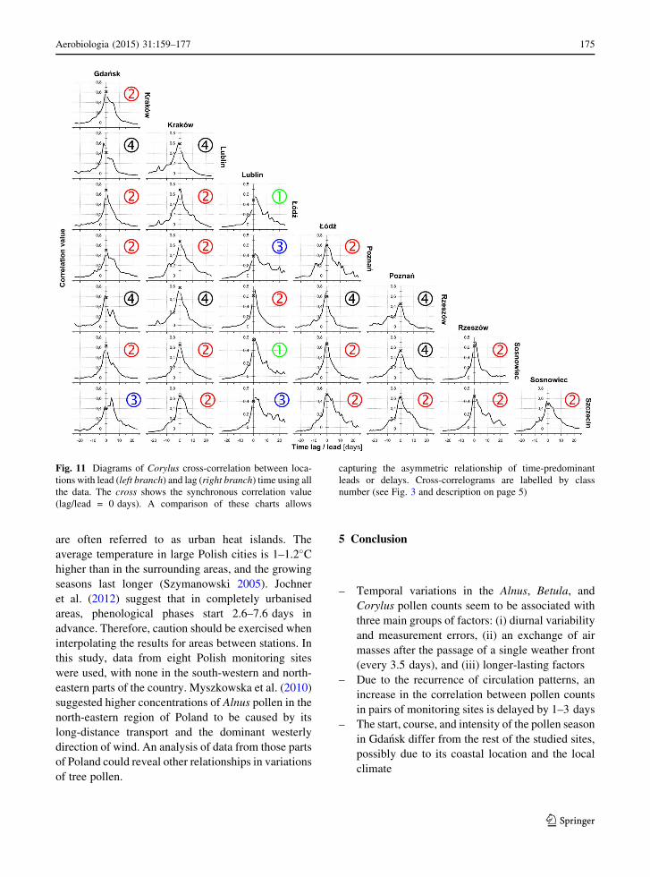
Fig. 11 Diagrams of Corylus cross-correlation between loca-
tions with lead (left branch) and lag (right branch) time using all
the data. The cross shows the synchronous correlation value
(lag/lead = 0 days). A comparison of these charts allows
capturing the asymmetric relationship of time-predominant
leads or delays. Cross-correlograms are labelled by class
number (see Fig. 3 and description on page 5)
Aerobiologia (2015) 31:159–177 175
123
– Three groups of locations connected with the local
topography and climate could be distinguished.
The first consists of the coastal cities, the second
group is linked with lowlands and highlands, and
the last group embraces those cities located in
southern Poland.
– It would be worthwhile to analyse the relationship
between variations in pollen counts and atmo-
spheric circulation patterns
Acknowledgments This study was carried out within the
framework of the projects no. NN305 321936 financed by the
Ministry of Science and Higher Education.
Open Access This article is distributed under the terms of the
Creative Commons Attribution License which permits any use,
distribution, and reproduction in any medium, provided the
original author(s) and the source are credited.
References
Accorsi, C. A., Bandini, M., Romano, B., Frenguelli, G., &
Mincigrucci, G. (1991). Allergenic pollen: Morphology
and microscopic photographs. In F. Spieksma, S. Bonini, &
G. D’Anato (Eds.), Allergenic pollen andpollinosis in
Europe. New York: Blackwell Scientific Publications.
Bleines, C., Deraisme, J., Geffroy, F., Jeannee, N., Perseval, S.,
Rambert, F., et al. (2011). Isatis technical references. Isatis
release 2011.
Bremer, B., Bremer, K., & Chase, M. (2009). An update of the
Angiosperm Phylogeny Group classification for the orders
and families of flowering plants: APG III. Botanical
Journal of the Linnean Society, 161(2), 105–121.
Chiles, J., & Delfiner, P. (2012). Geostatistics: Modeling Spatial
Uncertainty. New Jersey: Wiley Series in Probability and
Statistics: Wiley.
Comtois, P. (1998). Statistical analysis of aerobiological data. In
P. Comtois, V. Levizzani, & P. Mandrioli (Eds.), Methods
in aerobiology (pp. 217–258). Bologna: Pitagora Editrice
Bologna.
Corden, J., Stach, A., & Millington, W. (2002). A comparison of
Betula pollen seasons at two European sites; Derby, United
Kingdom and Poznan, Poland (1995–1999). Aerobiologia,
1996, 45–53.
Cowpertwait, P. S., & Metcalfe, A. V. (2010). Introductory time
series with R (Use R!). New York: Springer.
Dmochowska, H. (Ed.). (2013). Concise statistical yearbook of
Poland 2013. Warsaw: Statistical Publishing
Establishment.
Dyakowska, J. (1937). Researches on the rapidity of the falling
down of pollen of some trees. Polska Akademia
Umiejetnosci.
Emberlin, J., Mullins, J., Corden, J., Millington, W., Brooke, M.,
Savage, M., et al. (1997). The trend to earlier birch pollen
seasons in the U.K.: A biotic response to changes in
weather conditions? Grana, 36(1), 29–33. doi:10.1080/
00173139709362586.
Frenguelli, G. (2003). Basic microscopy, calculating the field of
view, scanning of slides, sources of error. Postepy Der-
matologii i Alergologii, 2, 227–229.
Garrison, B. A., Koenig, W. D., & Knops, J. M. H. (2006).
Spatial synchrony and temporal patterns in acorn produc-
tion of California Black Oaks. In: Proceedings of the 6th
symposium on Oak woodlands: Today’s challenges,
tomorrow’s opportunities PSW-GTR-217, pp. 343–356.
Goovaerts, P. (1997). Geostatistics for natural resources eval-
uation. Applied geostatistics series. Oxford: Oxford Uni-
versity Press.
Grewling, L., Jackowiak, B., Nowak, M., Uruska, A., & Smith,
M. (2012). Variations and trends of birch pollen seasons
during 15 years (1996–2010) in relation to weather con-
ditions in Poznan (western Poland). Grana, 51(4),
280–292. doi:10.1080/00173134.2012.700727.
Grewling, L., Sikoparija, B., Skjøth, C., Radisic, P., Apatini, D.,Magyar, D., et al. (2012). Variation in Artemisia pollen
seasons in Central and Eastern Europe. Agricultural and
Forest Meteorology, 160, 48–59. doi:10.1016/j.agrformet.
2012.02.013.
Hajkova, L., Nekovar, J., & Richterova, D. (2009). Temporal
and spatial variability in allergy-triggering phenological
phases of hazel and alder in Czechia. Folia Oecologica,
36(1), 8–19.
Heinzerling, L. M., Burbach, G. J., Edenharter, G., Bachert, C.,
Bindslev-Jensen, C., Bonini, S., et al. (2009). GA(2)LEN
skin test study I: GA(2)LEN harmonization of skin prick
testing: Novel sensitization patterns for inhalant allergens
in Europe. Allergy, 64(10), 1498–1506. doi:10.1111/j.
1398-9995.2009.02093.x.
Hirst, J. M. (1952). An automatic volumetric spore trap. Annals
of Applied Biology, 39(2), 257–265. doi:10.1111/j.1744-
7348.1952.tb00904.x.
Jochner, S. C., Sparks, T. H., Estrella, N., & Menzel, A. (2012).
The influence of altitude and urbanisation on trends and
mean dates in phenology (1980–2009). International
Journal of Biometeorology, 56(2), 387–394. doi:10.1007/
s00484-011-0444-3.
Kaszewski, B. M., Pidek, I. A., Piotrowska, K., & Weryszko-
Chmielewska, E. (2008). Annual pollen sums of Alnus in
Lublin and Roztocze in the years 2001–2007 against
selected meteorological parameters. Acta Agrobotanica,
61(2), 57–64. doi:10.5586/aa.2008.033.
Kluza-Wieloch, M., & Szewczak, J. (2006). Flowering phe-
nology of selected wind pollinated allergenic deciduous
tree species. Acta Agrobotanica, 59(1), 309–316.
Kotas, P., Twardosz, R., & Nieckarz, Z. (2013). Variability of
air mass occurrence in southern Poland (1951–2010).
Theoretical and Applied Climatology, 114(3–4), 615–623.
doi:10.1007/s00704-013-0861-9.
Leon Ruiz, E. J., Garcıa Mozo, H., Domınguez Vilches, E., &
Galan, C. (2012). The use of geostatistics in the study of
floral phenology of Vulpia geniculata (L.) Link. The Sci-
entific World Journal, 2012, 1–19. doi:10.1100/2012/
624247.
Liebhold, A., Sork, V., & Peltonen, M. (2003). Peltonen M
(2004) Within-population spatial synchrony in mast seed-ing of North American oaks. Oikos, 1, 156–164.
176 Aerobiologia (2015) 31:159–177
123

Lorenc, H. (2005). Atlas klimatu Polski. Warsaw: IMGW.
Malkiewicz, M., Klaczak, K., Drzeniecka-Osiadacz, A., Kryn-
icka, J., & Migała, K. (2013). Types of Artemisia pollen
season depending on the weather conditions in Wrocław
(Poland), 2002–2011. Aerobiologia. doi:10.1007/s10453-
013-9304-4.
Milewski, W. (Ed.). (2013). Forests in Poland 2012. Warsaw:
The State Forests Information Centre.
Mothes, N., & Valenta, R. (2004). Biology of tree pollen
allergens. Current Allergy and Asthma Reports, 4(5),
384–390.
Myszkowska, D., Jenner, B., Puc, M., Stach, A., Nowak, M., Mal-
kiewicz, M., et al. (2010). Spatial variations in the dynamics of
the Alnus and Corylus pollen seasons in Poland. Aerobiologia,
26(3), 209–221. doi:10.1007/s10453-010-9157-z.
Myszkowska, D., Jenner, B., Stepalska, D., & Czarnobilska,
E. (2011). The pollen season dynamics and the rela-
tionship among some season parameters (start, end,
annual total, season phases) in Krakow, Poland,
1991–2008. Aerobiologia, 27(3), 229–238. doi:10.1007/
s10453-010-9192-9.
Nilsson, S., & Persson, S. (1981). Tree pollen spectra in the
stockholm region (sweden), 1973–1980. Grana, 20(3),
179–182. doi:10.1080/00173138109427661.
Pannatier, Y. (1996). VARIOWIN software for spatial data
analysis in 2D/Yvan Pannatier. New York: Springer.
Piotrowska, K., & Kubik-Komar, A. (2012). The effect of
meteorological factors on airborne Betula pollen concen-
trations in Lublin (Poland). Aerobiologia, 28(4), 467–479.
doi:10.1007/s10453-012-9249-z.
Puc, M. (2003). Characterisation of pollen allergens. Annals of
Agricultural and Environmental Medicine: AAEM, 10(2),
143–149.
Puc, M. (2007). The effect of meteorological conditions on
hazel (Corylus spp.) and alder (Alnus spp.) pollen con-
centration in the air of Szczecin. Acta Agrobotanica, 60(2),
65–70. doi:10.5586/aa.2007.032.
Puc, M. (2012). Artificial neural network model of the rela-
tionship between Betula pollen and meteorological factors
in Szczecin (Poland). International Journal of Biometeo-
rology, 56(2), 395–401. doi:10.1007/s00484-011-0446-1.
R Core Team. (2013). R: A language and environment for sta-
tistical computing. R foundation for statistical computing,
Vienna, Austria. http://www.R-project.org/.
Ranta, H., & Satri, P. (2007). Synchronized inter-annual fluc-
tuation of flowering intensity affects the exposure to
allergenic tree pollen in North Europe. Grana, 46(4),
274–284. doi:10.1080/00173130701653079.
Rapiejko, P., Stankiewicz, W., Szczygielski, K., & Jurkiewicz, D.
(2007). Progowe ste _zenie pyłku roslin niezbedne do
wywołania objawow alergicznych. Otolaryngologia Polska,
61(4), 591–594. doi:10.1016/S0030-6657(07)70491-2.
Rasmussen, A. (2002). The effects of climate change on the
birch pollen season in Denmark. Aerobiologia, 18(3–4),
253–265. doi:10.1023/A:1021321615254.
Rodriguez-Rajo, F. J., Dopazo, A., & Jato, V. (2004). Envi-
ronmental factors affecting the start of pollen season and
concentrations of airborne Alnus pollen in two localities of
Galicia (NW Spain). Annals of Agricultural and Environ-
mental Medicine: AAEM, 11(1), 35–44.
Rodriguez-Rajo, F. J., Valencia-Barrera, R. M., Vega-Maray, A.
M., Suarez, F. J., Fernandez-Gonzalez, D., & Jato, V.
(2006). Prediction of airborne Alnus pollen concentration
by using ARIMA models. Annals of Agricultural and
Environmental Medicine: AAEM, 13(1), 25–32.
Rodriguez-Rajo, F. J., Grewling, L., Stach, A., & Smith, M.
(2009). Factors involved in the phenological mechanism of
Alnus flowering in Central Europe. Annals of Agricultural
and Environmental Medicine: AAEM, 16(2), 277–284.
Smith, M., Emberlin, J., Stach, A., Czarnecka-Operacz, M.,
Jenerowicz, D., & Silny, W. (2007). Regional importance
of Alnus pollen as an aeroallergen: A comparative study of
Alnus pollen counts from Worcester (UK) and Poznan
(Poland). Annals of Agricultural and Environmental
Medicine: AAEM, 14, 123–128.
Stach, A., Emberlin, J., Smith, M., Adams-Groom, B., & Mys-
zkowska, D. (2008). Factors that determine the severity of
Betula spp. pollen seasons in Poland (Poznan and Krakow)
and the United Kingdom (Worcester and London). Inter-
national Journal of Biometeorology, 52(4), 311–321.
doi:10.1007/s00484-007-0127-2.
Szymanowski, M. (2005). Miejska wyspa ciepła we Wrocławiu
[Urban heat island in Wrocław]. In: Studia Geograficzne—
tom 77, Wydawnictwo Uniwersytetu Wrocławskiego.
Ward Jr, J. H. (1963). Hierarchical grouping to optimize an
objective function. Journal of the American Statistical
Association.
Weryszko-Chmielewska, E., Puc, M., & Rapiejko, P. (2001).
Comparative analysis of pollen counts of Corylus, Alnus
and Betula in Szczecin, Warsaw and Lublin (2000–2001).
Annals of Agricultural and Environmental Medicine:
AAEM, 8(2), 235–240.
Ziello, C., Sparks, T. H., Estrella, N., Belmonte, J., Bergmann,
K. C., Bucher, E., et al. (2012). Changes to airborne pollen
counts across Europe. PloS one 7(4). doi:10.1371/journal.
pone.0034076.
Aerobiologia (2015) 31:159–177 177
123


