The Restoration of the Gold Standard after the US Civil War: A Volatility Analysis
Max Meulemann†, Martin Uebele‡ and Bernd Wilfling‡
20/2011
† Department of Economics, ETH Zürich, Switzerland ‡ Department of Economics, University of Münster, Germany
wissen•leben WWU Münster
The Restoration of the Gold Standard after the USCivil War: A Volatility Analysis
Max Meulemann∗, Martin Uebele†, Bernd Wilfling‡
This draft: February, 2011
Abstract
Using a Markov-switching GARCH model this paper analyzes the volatilityevolution of the greenback’s price in gold from after the Civil War until thereturn to gold convertibility in 1879. The econometric inference associatedwith our methodology indicates a switch to a regime of low volatility roughlyseven months before the actual resumption. Since this empirical finding ismost likely to be reconciled with a change in market expectations, we concludethat expectations affected the exchange rate more than fundamentals. Ouranalysis also demonstrates that regime switches in the volatility of exchangerates may reflect historical events that remain undiscovered otherwise.
Keywords: Monetary history; 19th century; USA; greenback; Markov-switching
GARCH models
∗Department of Economics, ETH Zurich, [email protected]†Department of Economics, University of Munster, [email protected]‡Department of Economics, University of Munster, [email protected]
1
1 Introduction
The Civil War was not only a decisive moment in American history but also a fun-
damental turning point in financial development. The return to the gold standard
constituted an important signal to financial markets worldwide since this monetary
regime was appreciated by almost all major countries until World War I and ul-
timately let the US dollar inherit the role of the leading world currency from the
British pound. However, within the U.S. bullionists and inflationists fought a fierce
political battle over the expected distributional consequences of either monetary
regime.
In this paper we study the period between the end of the American Civil War
and the return to gold in 1879 and contribute to the theoretical debate on the
factors that may drive exchange rates. In the literature covering this debate two
opposing opinions predominate. On the one hand, monetarists like Friedman and
Schwartz (1963) argue that exogenous macroeconomic fundamentals like money sup-
plies, price inflation and price parities cause the high premiums on gold. This view
is supported, inter alia, by Kindahl (1961), and Officer (1981). On the other hand,
Calomiris (1992, 1988, 1985) strongly opposes this view by stating that expectations
are more important to the greenback exchange rate than the classical fundamen-
tals (like money supplies). Consequently, Calomiris supports the research pursued,
among others, by Mitchell (1903) and Willard, Guinnane, and Rosen (1996) who
attempt to incorporate news and significant events in their study of the greenback
markets. However, besides these opposing views other authors (e.g. Smith and
Smith, 1997) argue that both expectations and macroeconomic fundamentals did
play a role in the evolution of the greenback exchange rate.
In this paper we make contributions to both the financial history of the U.S. and
to the debate on the factors that drive exchange rates. To this end we implement a
so-called Markov-switching GARCH model that has recently emerged in the macro-
finance literature (see for example Wilfling, 2009) and which enables us to analyze
1
time-varying conditional variances of daily greenback-gold exchange rates.
More explicitly our methodology helps us to identify distinct phases (regimes)
of high and low exchange-rate volatility. Since such distinct exchange-rate volatility
regimes can easily be reconciled with market participants’ expectations on future
changes in the exchange rate (rather than with changes in fundamentals), we inter-
pret our results as empirical evidence that agents had anticipated the exchange-rate
fixing associated with the return to the gold standard beforehand. In particular,
our econometric analysis detects a regime switch from high to low exchange-rate
volatility several months before the actual resumption thus supporting Calomiris’
view that expectations may have mattered more than macroeconomic fundamentals.
Our econometric technique also provides a new means of gauging the Civil War
and the postbellum period. Initially, from a financial investor’s perspective, our
results reflect the considerable political uncertainty that characterized the postbel-
lum years. However, the switch to a low volatility regime long before the actual
resumption date demonstrates that policy makers were surprisingly able to commit
to their announced resumption plan.
This paper contains 6 sections. In Section 2 we briefly review the histori-
cal background for which we rely on some of the established historical literature
(e.g. Mitchell, 1903; Friedman and Schwartz, 1963; Unger, 1964) . Section 3 presents
our data set. In Section 4 we specify our econometric model in the form of a two-
regime Markov-switching GARCH model. Section 5 presents the estimation results
while Section 6 offers some concluding remarks.
2 Historical Background
Before the Civil War the U.S. money supply consisted of gold and silver coins,
copper pennies and notes issued by state or private banks. All non-specie money
could principally be converted into gold. There was no paper money issued by the
government. However, the U.S. was practically on a gold standard since the relative
2
price of gold to silver was higher than the world-market price so that not many silver
coins were in circulation. Unlike today, there was no strong banking and currency
system and no Federal Banking System in the U.S. More than 1,600 state banks
existed all over the country and more than 7,000 different kinds of bank notes were
in circulation the half of which carried no real worth.
At the beginning of the Civil War the Unionist government encountered difficul-
ties in selling sufficient bonds to finance its war efforts, which lead to the suspension
of specie payment by private banks and the government on December 30, 1861. This
was partly due to the increased war expenditures and the low confidence in public
securities and to some extent to the lack of confidence in the government and the
prospects of the war. These were gravely tampered by the danger of a war with the
United Kingdom because of the Trent affair (an incident in which two Confederate
envoys were captured from the British Mail steamer Trent). The government reacted
by issuing an inconvertible currency which became rapidly known as the ‘greenback’
to cover war expenditures. Three Legal Tender Acts in February 1862, July 1862,
and in January 1863 put around $450 million greenbacks into circulation.
However, since transactions with foreigners and the payment of customs duties
and tariffs required gold, greenbacks did not constitute a perfect substitute for gold
dollars. Consequently, a market emerged soon after the greenback issuance and the
greenbacks depreciated from par, the main reasons for the depreciation being the
increased demand induced by the government’s war spending, the expansionist fiscal
policy, negative trade balances and also war news. Bad news induced hoarding in
an expectation of a higher gold price while good news prompted people to sell gold
in anticipation of declining prices. Nevertheless, contemporaries believed this to be
a temporary measure and the parity to be restored after the war, although nothing
had been specifically declared. Meanwhile, greenbacks served as legal tender in most
parts of the country where prices were quoted in greenbacks and gold was valued
at its current premium market price. Only at the West Coast prices were quoted in
3
gold and discounted to greenback prices at the current market value.
The time after the Civil War saw a huge decline in commodity prices which may
be ascribed to the contraction efforts undertaken by the Secretary of the Treasury,
Hugh McCulloch. These efforts were affirmed by the Congress in December 1865,
but later restricted by the Congress in April 1866 and finally completely ceased in
1868. In addition, ‘natural growth’ reduced price levels as the money stock was held
fairly stable.
Three legal decisions in 1868 reduced the role of greenbacks in business trans-
actions. (1) In Lane Country vs. Oregon it was ruled that state taxes could only
be paid in specie, but not in legal tender notes. (2) In Bronson vs. Rhodes the
Supreme Court decided that contracts demanding payment only in specie were le-
gal. (3) In Bank of New York vs. Board of Supervisors the state was denied to levy
property taxes on state notes which meant that the court did not consider them
as money. The decision about the legal status of greenbacks was engaged by the
Supreme Court in 1869. Initially it was ruled under Chief Justice Chase (who him-
self at that time had issued the Legal Tender Acts) that greenbacks had no legal
tender status for contracts before the Legal Tender Acts. Owing to the accession
of two new members to the court, this decision was reversed in 1871 when it was
ruled that the government had the right to issue legal tender notes. However, the
issue was not settled before 1884 when it was ruled that the government was eligible
to do so also in times of peace. The government’s commitment to debt payment in
coin was shown when President Grant came to power and the gold-payment bill was
enacted – which obliged the government to pay its debt in specie.
In the fall of 1873, the railroad boom suddenly came to an end and the subsequent
banking panic marked the beginning of a crisis in most parts of the country. For the
rest of the decade the currency problem and the conduct of financial policy became
the issues of major public and political concern. President Grant was cautious
in following either expansionary or contractionary monetary stances, an attitude
4
that deeply confused the public opinion. Mixon (2006), for example, reports that
the business community characterized the situation as ‘frustrating, uncertain, and
unclear, and the finger of blame is clearly pointed at the government.’
After a period of controversial debate the Inflation Bill finally emerged in 1874.
The bill was to provide for additional national bank note circulation and to return
to the $400 million of greenbacks which had circulated before the contraction mea-
sures in the 1860s. It was intended to resume specie payment on January 1, 1876.
Although a rather modest measure, it represented a retreat from the resumption
policy and therefore conservatives appealed to Grant to veto the law. On April 22
Grant gave his veto to the bill which for the public opinion came like a ‘bombshell.’
In the aftermath, the Republican Party fell into a state of great disunity and for
the first time since 1861 the Party lost the majority in Congress. Therefore, the
Republicans were eager to restore their unity and enacted the Resumption Act dur-
ing the lame-duck session after the congressional elections in 1874. Fearing another
presidential veto and the upcoming presidential elections, the Republican Senatorial
caucus tried to realign inflationists and conservatives on a compromise that both
sides could accept. In the wake of this free banking was introduced as a major
concession to the soft money faction and inflationists since it allowed controlled in-
flation and a promotion of the national banking system. In addition to this, $80
of greenbacks were to be redeemed in exchange for each $100 bank note until only
$300 million were supposed to be left. Resumption was proposed for January 1,
1879. Compared to the vetoed Inflation Bill the proposal itself did not constitute a
real innovation, but the resumption was put exactly three years later on January 1,
1879 and many observers did not assess this decision as final.
Although the Presidential Election in 1876 loomed dark over the country and the
Republican Party, it was finally decided by aspects like railroad issues and patronage.
After Rutherford B. Hayes, the Republican candidate, had won by a margin of one
electoral vote the White House was commanded by a Republican, the House of
5
Representatives by the Democrats, while the Senate was in a stalemate. Hayes, a
well-known sound-money representative, appointed John Sherman as Secretary of
the Treasury. Sherman, from then on in charge of the accomplishment of resumption,
believed that he needed at least an amount of gold large enough to be able to redeem
40 per cent of the outstanding greenbacks. This appeared to be a difficult task since
at the same time Germany and France were in dire need of gold themselves. He
proved to be up to the task by offering bonds with higher interest rates to foreigners
and prevented a critical drain on the money market by increasing deposits in national
banks. An attempt to repeal the Resumption Act passed the Congress, but was
declined in the Senate by one vote. The Bland Allison Acts of 1877 and 1878 and
the Coinage Act in May 1878 constituted the final attempts to avert resumption,
but did not endanger the resumption policy or change the legal commitment to
resume specie payment on January 1, 1879. The crop failures in Europe injected
large amounts of gold into the U.S. and activated the U.S. trade balance from 1876
onwards. Sherman secured this inflow of gold by selling gold bonds and by November
1878 he had built up a gold reserve of around $141.9 million. The premium on gold
fell constantly and on December 17, 1878 par had been reached for the first time
since 1862. In the days after resumption only a few notes were redeemed and in fact
more gold was exchanged for paper money. Although this might be considered as a
victory of the hard money faction the issue had definitely not been settled yet. More
than $346 million wartime greenbacks and an annually increasing amount of silver
certificates still threatened the gold standard. The reserve of around $100 million
gold dollars could only maintain the gold standard as long as the country remained
prosperous and the important task of the subsequent government was to secure the
gold standard. However, Calomiris (1992) demonstrates that fear about inflation
remained by reporting expected inflation rates to be higher than real inflation rates.
In a similar vein, Studenski and Krooss (2003) perceives the risk that silver could be
used to pay government obligations and that gold could be drawn from the Treasury
6
reserves and exported.
3 Data
3.1 Data Origin
For about two weeks after the suspension of the gold standard there was no official
market for gold in New York. People willing to buy or sell gold needed to appeal to
foreign coin dealers until this business became too voluminous to be conducted in
such an unorganized way. The first organized gold trading started at the New York
Stock Exchange on January 13, 1862. A competing trading place was established in
a ‘dingy cellar’ in William Street dubbed the ‘coal hole’ (see Mitchell, 1903). As the
business became larger the market moved first into the Gilpin’s News Room, later
into the old stock board at No. 24 Beaver Street, and finally into New Street next to
the Stock Exchange. The traders in this market started referring to it as the ‘Gold
Room’ and were content with the loose organization. It was not before October
1864 that a constitution and by-laws were adopted and regular officers elected. It
is noteworthy that trading gold for other than commercial reasons at the New York
Stock Exchange was considered unpatriotic or a bet against the Union’s victory.
This appeared in contrast to the Gold Room where speculations were not shunned
at (see Nugent, 1968).
The transaction volumes in these and in two other markets were reported to be
large. Importers and exporters had to change paper currency and gold to buy and
sell goods, but also tried to protect themselves against fluctuations of the currency’s
value while awaiting the execution of their contracts. In fact, Mitchell (1903, pp.
182-185) believed that the volume of speculation exceeded normal transactions by
far. However, speculators were not cherished by everyone as clarified by Willard,
Guinnane, and Rosen (1996) quoting Abraham Lincoln’s dictum on gold market
traders: ‘I wish every one of them had his devilish head shot off!’
Since the prices from the New York gold markets were telegraphed to all other
7
important U.S. cities and regarded as authoritative, we neglect prices from other
cities. First sources of our data are financial columns of daily papers like the Hunt’s
Merchant Magazine, the Bankers’ Magazine or the Commercial and Financial Chron-
icle. Typically, these sources report daily highest, lowest, and closing prices. There
are similar tables from the Chamber of Commerce of the State New York as well as
yearly published almanacs by other newspapers. However, the main source were the
detailed reports by J.C. Mersereau, Register of the Gold Exchange, who published
an annual book called ‘American Gold, 1862-(date of issue)’. This book gave the
quotations from 10 a.m. until 3 p.m. for every quarter of an hour.
All sources combined did not deviate by much and Mitchell (1908) checked them
for typos. He collated the data based on Mersereau’s latest issue from 1878 with
the tables from the Commercial and Financial Chronicle from which he took the
data for the last year 1878. Finally, the first two weeks were taken from New York’s
daily papers so that the complete data set contains 5,170 daily observations of the
greenback/gold dollar exchange rate for the whole period from 1862 until 1879.
The exchange rates are given in indirect quotation meaning that $100 greenback
were exchanged for a given sum of gold dollars. For example, on January 2, 1863 $100
greenback were exchanged on average for $74.77 in gold. Mitchell (1908) compiled
all his data in the book ‘Gold, prices, and wages under the greenback standard’.1
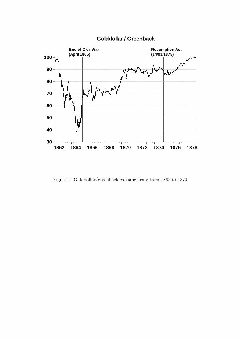
Figure 1 about here
3.2 Data Description
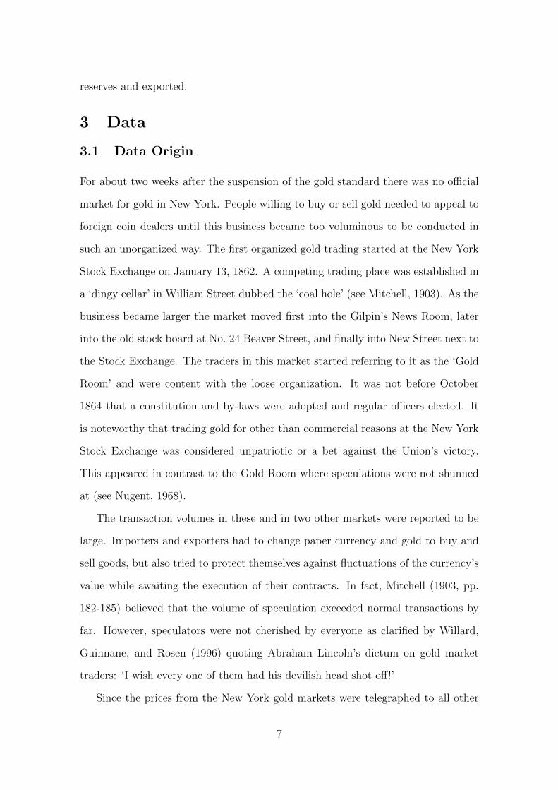
Figure 1 displays the golddollar/greenback exchange rate between 1862 and 1879.
In mid-1864 the exchange rate dropped to only 37% of its face value and steadily
recovered afterwards. The first vertical marking represents the end of the Civil
War around April 9, 1865 while the second marking shows the enactment of the
1The data can be accessed online at http://EH.net/databases/greenback.
8
Resumption Act on January 14, 1875.2
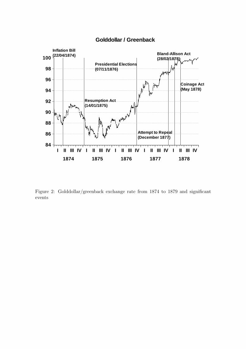
Figure 2 about here
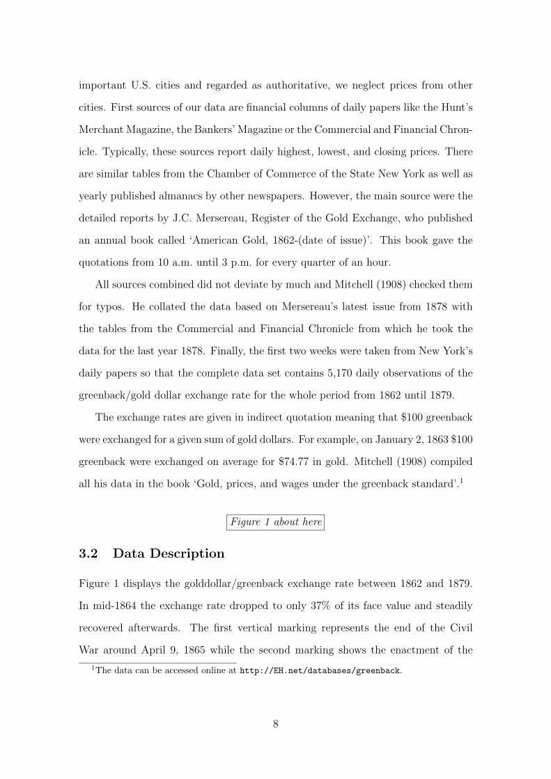
Figure 2 displays the evolution of the golddollar/greenback exchange rate dur-
ing the years 1874 to 1879. The reason for considering this shortened time interval
is that we aim at locating the switch to a regime of low volatility around the an-
nouncement date January 14, 1875. Shortly after Grant’s Veto the greenback’s
value appreciated, but then again fell steadily for several months (see the first verti-
cal marking). Overall, this period was characterized by high uncertainty about the
upcoming financial policy and possibly financial market participants were initially
relieved that the Resumption Act was considered to be an inflationist measure in
the short run. The second vertical line marks the day of the Resumption Act on
which the greenback price fell. The price went on falling and remained low for more
than six months before it suddenly peaked in September 1875. The exchange-rate
dynamics directly following the Resumption Act may be interpreted as evidence
that in the beginning the resumption did not affect financial markets substantially.
The third vertical marking represents Hayes’s victory of the presidential elections.
From then on the exchange rate appears to be trending upwards. Although Unger
(1964) reports that the financial question had not been of major public concern
during the elections, we interpret this exchange-rate dynamics as evidence that
Hayes’ hard money reputation actually affected the time series.
In spite of their political relevance the last three events represented by vertical
markings did not affect exchange-rate dynamics considerably. The failure of repeal
in 1877 had the potential to be the decisive hit against sound money opposition
and it appears that the appreciation was only delayed by this decision in favor of
the resumption. The steps taken later in 1878 had no substantial effect on the
2There still is controversy on the exact day dating the end of the Civil War. For an overviewtreating the significant events of the Civil War see Rhodes (1999).
9
legal commitment of resumption so that the greenback steadily continued to trend
upwards towards par.
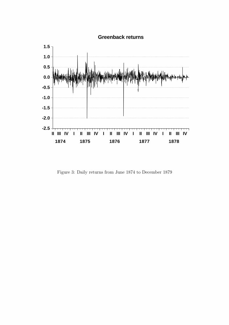
Figure 3 about here
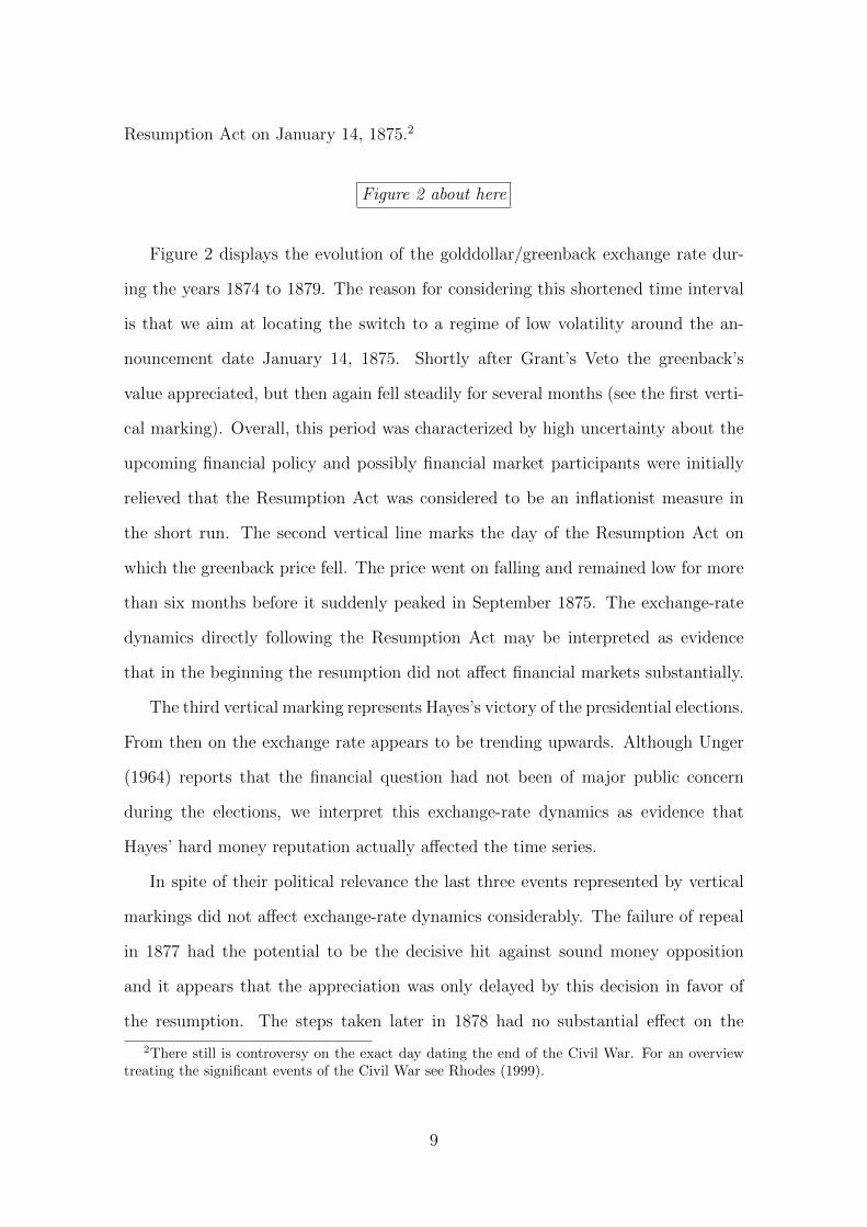
Figure 3 displays the daily exchange-rate returns defined as 100·[ln(xt)−ln(xt−1)]
for the time between June 1, 1874 and December 31, 1879 amounting to a total of
1394 observations. Mere visual inspection of the return series reveals a regime of
declining exchange-rate volatility beginning in spring 1878 with the returns falling
to an extremely low level several months before the resumption. The mean of the
exchange-rate returns appears to fluctuate randomly around zero.
In a first preliminary statistical analysis we split the whole sample into two
equally large portions and compared the means and the standard deviations of both
subsamples. While the two subsample means only differ slightly from each other,
the standard deviations of both subsamples are given by σ1 = 0.21 and σ2=0.15 and
appear to be significantly different from each other. This difference in the standard
deviations becomes even larger if we modify both subsamples by considering the
first subsample ranging from June 1874 until April 1878 and the second subsample
ranging from May 1878 until December 1878. In this case both standard deviations
are given by σ1 = 0.20 and σ2 = 0.067 hinting at a low volatility regime at the end
of the sample, a finding that is consistent with our conjecture described above.
4 Econometric Technique
4.1 Motivating Switching Volatility Regimes in the Dynam-ics of the Golddollar/Greenback Exchange-Rate
In this section we provide an explanation for why we expect to find distinct volatility
regimes in the nominal golddollar/greenback exchange-rate data described above.
Our explanation rests on the fact that the return to the gold standard marked
a transition between two alternative exchange-rate systems. Before the return to
10
gold the exchange rate floated freely reflecting changes in the relative supply-to-
demand conditions of the currencies involved while the return to gold represented
the introduction of a system of completely fixed rates. Bearing this transition in
mind we invoke the existing literature on exchange-rate dynamics under alternative
exchange-rate systems and under consecutive international monetary regimes which
provides a theory-based motivation for switching volatility regimes in our time-series
data.
Several authors have analyzed a transition from a system of floating exchange
rates into a fixed-rate system on a given future date and at publicly announced
fixing-parity. Under rational expectations, the mere knowledge in the market that
the presently floating exchange rate will be irreversibly fixed in the future does affect
the exchange-rate dynamics prior to the fixing. Theoretical models of exchange-
rate dynamics under such a scenario have been developed by Miller and Sutherland
(1994), Sutherland (1995), DeGrauwe et al. (1999) and Wilfling and Maennig (2001).
Although focusing on different aspects, all papers derive the same unambiguous
result: at that moment when the authorities publicly announce the future exchange-
rate fixing the spot rate jumps from its floating-path onto an interim-path which
assures an arbitrage-free transition into the fixed-rate system.
The analytical form of the interim-path crucially hinges on the political and in-
stitutional framework during the run-up to the fixed-rate system. However, Wilfling
and Maennig (2001) analyze a setting in which foreign exchange market participants
may be uncertain about the authorities’ adherence to the publicly announced fixing
date, that is, in which agents take account of the fact that the beginning of the
fixed-rate system may be delayed. Two results concerning (conditional) exchange-
rate volatility along the interim-path are apparent from their model. (1) The mere
announcement of future exchange-rate fixing reduces exchange-rate volatility along
the interim path. This volatility reduction is certain, even in a setting with market
uncertainty about the punctual entrance into the fixed-rate system. Only in the ab-
11
solutely extreme case in which agents believe that the fixed-rate system will never
be implemented, exchange-rate volatility remains unaffected by the announcement.
(2) The volatility reduction along the interim-path is maximal when agents assess
the political announcement as fully credible, that is, if they are convinced that the
exchange-rate fixing will occur punctually at the previously specified future date.
Overall, an essential feature of the Wilfling and Maennig (2001) model is that
there are two extreme volatility regimes during the run-up to the fixed-rate system:
(1) an extreme high-volatility regime, during which agents are either not aware of
the future exchange-rate fixing or believe that the fixed-rate system will never be
implemented, and (2), an extreme low-volatility regime during which agents are
absolutely convinced that the exchange-rate fixing will start according to schedule.
Apart from the economically well-grounded statements on the distinct volatility
regimes, the Wilfling and Maennig (2001) model rests on an assumption that may
appear unrealistic at first glance. Their model assumes that there is a clear-cut
date (the so-called announcement date) at which the future exchange-rate fixing is
announced and that this announcement comes as a surprise to market participants.
In reality, however, inspired by political debates and perceptible institutional pro-
cesses, agents frequently form expectations about the punctual fixing long before
any definite official announcement.
A straightforward way to overcome this inconsistency is to reinterpret the an-
nouncement date from the theoretical model as the date-of-first-notice, that is, as
the date at which market participants perceive a potential future exchange-rate fix-
ing for the first time. Starting from this date, agents deem a shift from presently
floating to fixed exchange rates possible and continuously assess the likelihood that
the fixing will occur punctually at the given date. This phase of uncertainty revisions
will typically last for a while until market participants are absolutely convinced that
the exchange-rate fixing will happen according to schedule. In what follows, the ear-
liest moment from which onwards agents are absolutely convinced of the punctual
12
exchange-rate fixing will be termed the date-of-full-acceptance.
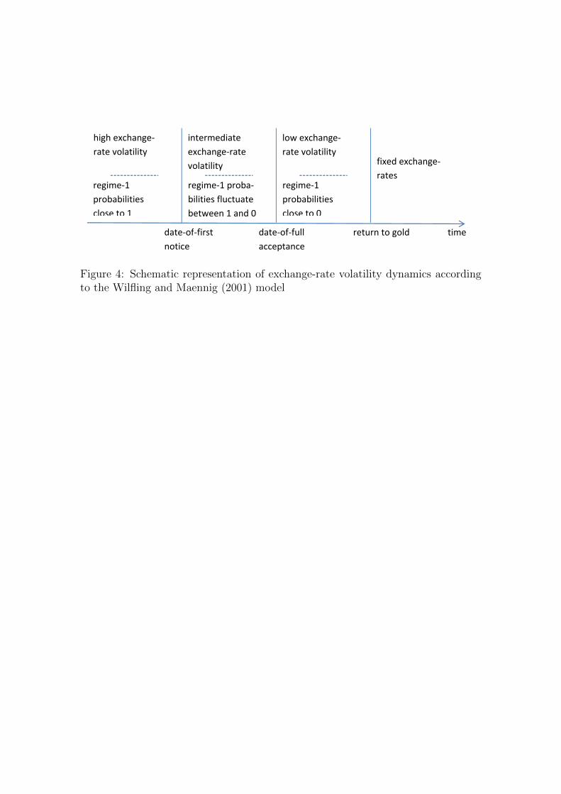
Figure 4 about here
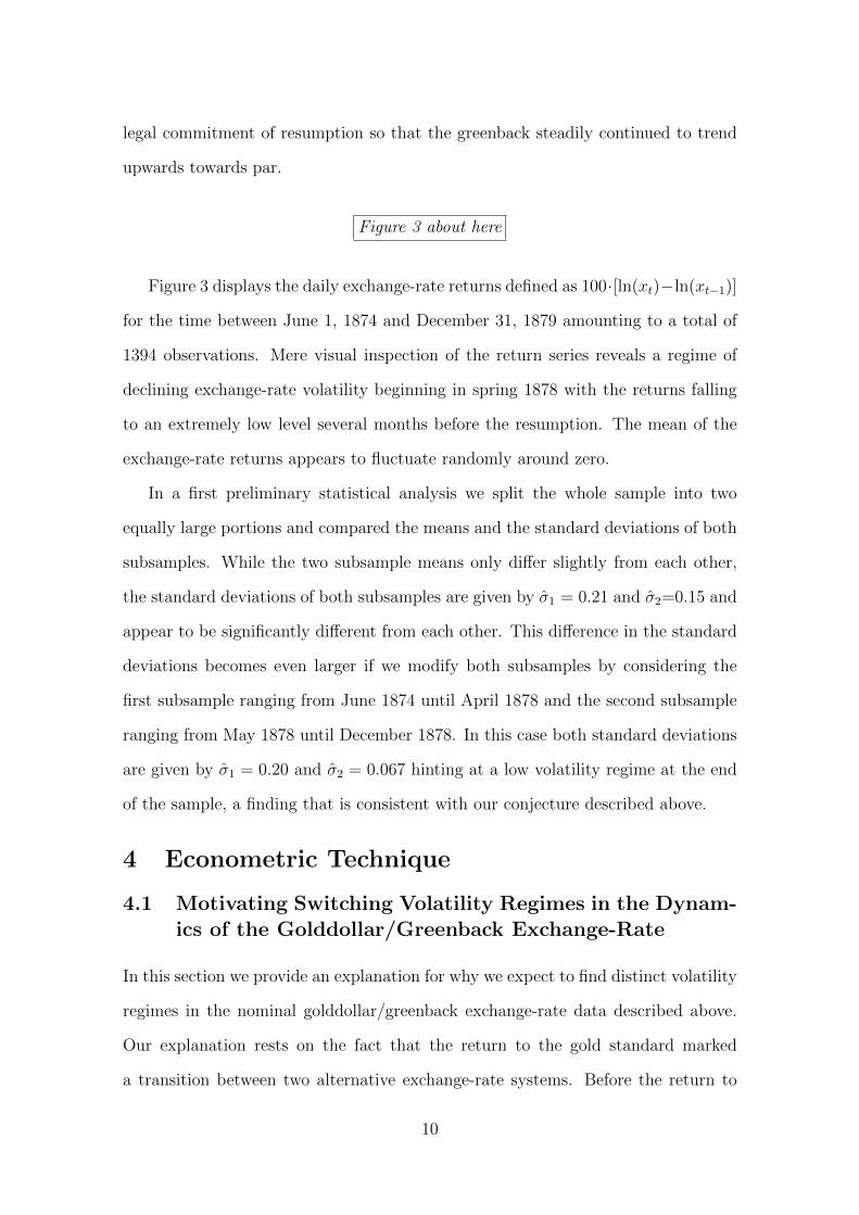
Figure 4 displays the schematic representation of the exchange-rate volatility
dynamics prior to the return to the gold standard as predicted by the theoretical
Wilfling and Maennig (2001) model. Before the date-of-first-notice agents believe
that the currently existing system of freely floating exchange rates will hold forever
so that exchange-rate volatility is high (extreme high-volatility regime). Next, we
consider the time between the date-of-full-acceptance and the return to gold. Dur-
ing this period, all uncertainty about the punctual fixing will have been completely
resolved so that exchange-rate volatility should be low and, according to the theo-
retical model, should converge to zero shortly before the implementation of the gold
standard (extreme low-volatility regime). Finally, we consider the time between
the date-of-first-notice and the date-of-full acceptance during which agents begin to
incorporate the potential future exchange rate fixing into their currency valuation
schemes, but—owing to relevant news—more or less frequently modify their assess-
ments about the punctual return to the gold standard. Depending on the changes
in these assessments, this period is typically characterized by news-induced switches
between high and low exchange-rate volatility regimes. Wilfling and Maennig (2001)
derive analytical formulas for the conditional exchange-rate volatility during this pe-
riod of uncertainty. They also prove that exchange-rate volatility during this period
strictly lies between the volatility levels from the above-described high- and the
low-volatility regimes what justifies the notion ‘intermediate exchange-rate volatil-
ity’ used in Figure 4.
Finally, it should be noted that the date-of-first-notice and the date-of-full-
acceptance are both free to vary along the time axis in Figure 4 so that this frame-
work covers a broad range of possible scenarios. For example, both dates will co-
incide if market participants perceive a prospective return to the gold standard for
13
the first time and are immediately convinced that the exchange-rate fixing will start
as officially scheduled. An alternative scenario involves a considerable extent of un-
certainty about the return to gold that may remain until the actual institutional
implementation of the gold standard. In this case, the date-of-full-acceptance would
coincide with the return to gold.
However, although theoretically possible, it is not very likely that the market
uncertainty characterizing the period between the date-of-first-notice and the date-
of-full-acceptance lasts for a very long time in real-world situations. Moreover, since
the corresponding volatility levels necessarily range between the volatility levels of
the extreme regimes, we waive modeling such intermediate regimes and focus on
the detection of the two extreme volatility regimes in our subsequent econometric
analysis.
4.2 A Markov-Switching GARCH Model
In order to model the two distinct volatility regimes in our exchange-rate return
series {Rt} which we define as
Rt = 100 · [ln(Xt)− ln(Xt−1)], (1)
we make use of a Markov-switching-GARCH model as developed in Gray (1996b)
and recently refined in Wilfling (2009) and Gelman and Wilfling (2009). The general
idea behind this econometric framework is that the data-generating process (DGP)
of the return Rt is affected by a latent random variable which represents the state
the DGP is in on any particular date t. In our analysis we denote this latent state
variable by St and use it to discriminate between the two distinct volatility regimes.
We specify St = 1 to indicate that the DGP is in the high-volatility regime whereas
St = 2 is meant to indicate that the DGP is in the low-volatility regime.
The basic element of our Markov-switching-GARCH model is the well-known
probability density function of a mean-shifted t-distribution with ν degrees of free-
14
dom, mean µ and variance h, tν,µ,h. Based on this parametric density function, our
next step will consist in specifying stochastic processes for the mean and the volatil-
ity in regime i, denoted by µit and hit, according to which the exchange-rate return
Rt is generated conditional upon the regime indicator St = i, i = 1, 2. After having
specified µit and hit we can then represent the conditional distribution of the return
as a mixture of two mean-shifted t-distributions:
Rt|φt−1 ∼
{tν1,µ1t,h1t with probability p1t
tν2,µ2t,h2t with probability (1− p1t), (2)
where φt−1 defines the information set as of date t − 1 and p1t ≡ Pr{St = 1|φt−1}
denotes the so-called ex-ante probability of being in regime 1 at time t.
In modeling our regime-dependent mean equation, we consider a simple form by
assuming a first-order autoregressive process (AR(1)-process) in each regime yielding
µit = a0i + a1i ·Rt−1 for i = 1, 2. (3)
In contrast to the mean equation (3), the specification of an adequate GARCH
process for the regime-specific variance hit is more problematic. Without going into
technical detail, we first consider an aggregate of conditional return variances from
both regimes at date t:3
ht = E[R2t |φt−1
]− {E [Rt|φt−1]}2
= p1t(µ21t + h1t
)+ (1− p1t) ·
(µ22t + h2t
)− [p1tµ1t + (1− p1t)µ2t]
2 . (4)
The quantity ht now provides the basis for the specification of the regime-specific
conditional variances hit+1, i = 1, 2 in the form of a parsimonious GARCH(1,1)-
structure. More explicitly, we follow the suggestion in Dueker (1997) and first pa-
rameterize the degrees of freedom of the tν,µ,h-distribution by q = 1/ν, so that
3See Gray (1996b) for a rigorous formal discussion.
15
(1− 2q) = (ν − 2)/ν, and then specify our regime-specific GARCH equation as
hit = b0i + b1i(1− 2qi)ε2t−1 + b2iht−1 (5)
with ht−1 as being given according to Eq. (4) and εt−1 being obtained from
εt−1 = Rt−1 − E [Rt−1|φt−2]
= Rt−1 − [p1t−1µ1t−1 + (1− p1t−1)µ2t−1] . (6)
It is important to note here that for i = 1, 2 the sums b1i(1 − 2qi) + b2i of
the coefficients from Eq. (5) constitute convenient measures of the regime-specific
persistence of volatility shocks. The higher the value of this measure the more time
it takes until a shock dies out. A regime-specific volatility shock will die out in
finite time if the coefficient sum is less than 1. For the case of the coefficient sum
being equal to 1 (i.e. for an integrated GARCH(1,1) process) volatility shocks have
a permanent effect and the unconditional variance of the process becomes infinitely
large.
Finally, we close our Markov-switching-GARCH model by parameterizing the
regime indicator St as a first-order Markov process with constant transition prob-
abilities. Denoting by πi the probability of the DGP persisting in regime i (for
i = 1, 2) between the dates t− 1 and t, we specify
Pr {St = 1|St−1 = 1} = π1, Pr {St = 2|St−1 = 1} = 1− π1,
Pr {St = 2|St−1 = 2} = π2, Pr {St = 1|St−1 = 2} = 1− π2.(7)
Now, the log-likelihood function of our Markov-switching-GARCH(1,1) model
can be obtained by performing similar calculations as in Gray (1996b). The exact
form of the function is presented in Wilfling (2009). The log-likelihood function
contains the ex-ante probabilities p1t ≡ Pr{St = 1|φt−1} which can be estimated
via a recursive scheme. These probabilities are useful in forecasting one-step-ahead
regimes based on an information set that evolves over time. In our context, the
16
ex-ante probabilities p1t reflect current market perceptions of the one-step-ahead
volatility regime, thus representing an adequate measure of foreign exchange market
volatility sentiments. Besides the ex-ante probabilities p1t we also address the so-
called smoothed probabilities Pr{St = 1|φT} which can be computed by the use of
filter techniques after the model estimation has been carried out.4 The smoothed
probabilities are based on the full sample-information set φT and provide a tool for
inferring ex post if and when volatility regime switches have occurred in the sample.
Table 1 about here
5 Estimation Results
Table 1 presents the maximum-likelihood estimates of our Markov-switching GARCH
model. Maximization of the log-likelihood function was performed by the ‘MAXI-
MIZE’-routine within the software package RATS 6.1 using the BFGS-algorithm,
heteroscedasticity-consistent estimates of standard errors and suitably chosen start-
ing values for all parameters involved. In contrast to our theoretical mean equation
(3) we estimated an AR(1)-process with identical, non-switching parameters across
both regimes. We imposed the simplifying restriction a01 = a02 and a11 = a12 for two
reasons, namely (1) in order to reduce the number of parameters to be estimated,
and (2) to focus on the volatility features of the exchange-rate returns. Overall, we
find that 9 out 12 parameters from our mean and GARCH equations (3) and (5)
are statistically significant at the 1% level.5
The GARCH parameters of regime 1, b01, b11, b21 appear much larger than their
4In this paper, we have computed all smoothed probabilities with a filter algorithm provided byGray (1996a).
5Some comments on the probability distribution of the conventional t-statistic within ourMarkov-switching-GARCH framework are in order. It has to be noted that the exact finite-sample distribution of our t-statistics is generally unknown. However, owing to some well-knownasymptotic properties of general maximum-likelihood estimators in conjunction with an appro-priate limiting-distribution result, it can be concluded that under the null hypothesis of a singleparameter being equal to zero, our t-statistics should converge in distribution towards a standardnormal variate. This implies asymptotic critical values of 2.58, 1.96 and 1.64 for the absolute valueof the t-statistic at the 1, 5, and 10%-levels, respectively.
17
corresponding counterparts b02, b12, b22 in regime 2. In conjunction with the (modi-
fied) degree-of-freedom parameters q1 and q2 the regime-specific volatility persistence
measures b1i(1− 2qi) + b2i are given by 0.6615 in regime 1 and 8.3 · 10−6 in regime
2 indicating a substantially higher degree of volatility persistence in regime 1 than
in regime 2. However, both volatility persistence measures are less than 1 which
suggests stationary conditional volatility processes in both regimes implying that
regime-specific volatility shocks die out in finite time. The estimates of the transi-
tion probabilities are given by π1 = 0.9776 and π2 = 0.8096 indicating a particularly
high degree of regime persistence for regime 1.
Apart from parameter estimation we also performed several specification tests
and diagnostic checks of the model fit. Inter alia, we tested for serial correlation of
the squared standardized residuals for the lags 1, 2, 3, and 5 with the well-known
Ljung-Box-Q-test finding that the null hypothesis of no autocorrelation cannot be
rejected up to lag 5 at any conventional significance level. This result provides some
evidence in favor of our two-regime Markov-switching GARCH specification.6
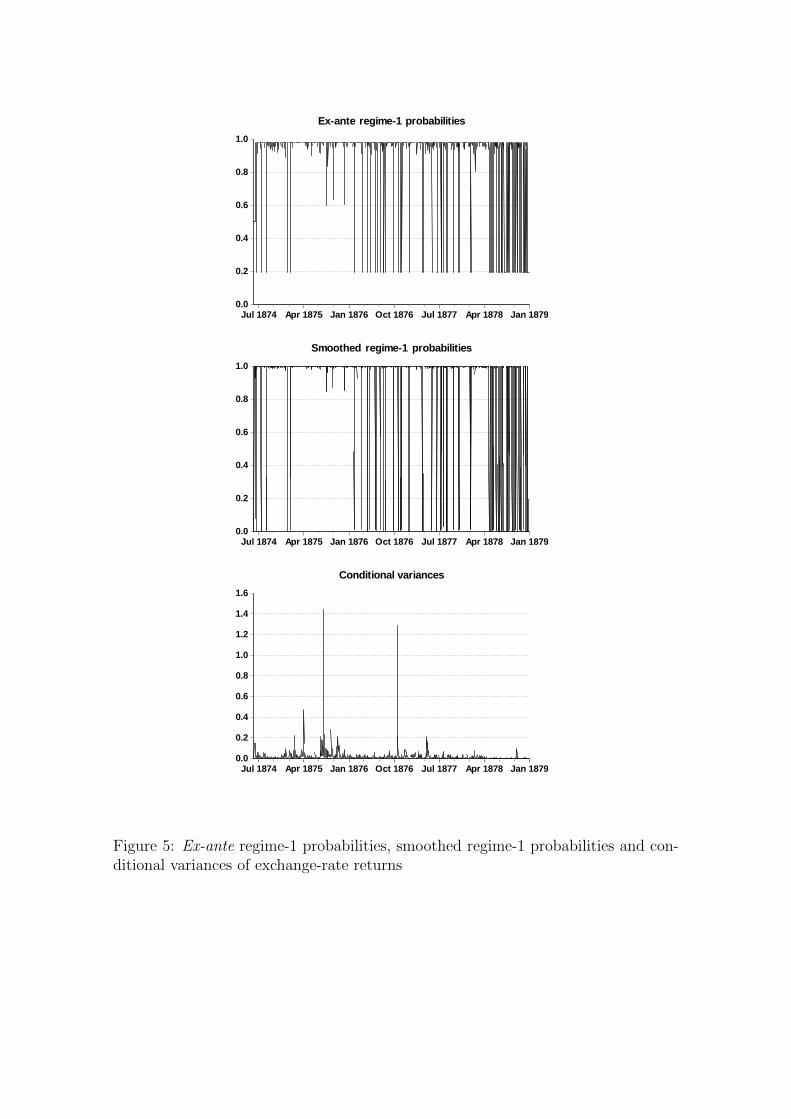
Figure 5 about here
Next, we address the ex-ante and the smoothed probabilities Pr{St = 1|φt} and
Pr{St = 1|φT} both of which are relevant to detecting how often and at which
dates the exchange-rate returns switched between the high-volatility and the low-
volatility regimes. Figure 5 displays these regime-1 probabilities (in the upper pan-
els) along with the conditional variance process (in the lower panel) estimated from
our Markov-switching GARCH model.
Theoretically, we would expect to observe dynamics of the regime-1 probabilities
(more concretely of both the ex-ante as well as the smoothed regime-1 probabil-
ities) in line with the schematic representation depicted in Figure 4. Before the
date-of-first notice exchange-rate volatility is high and, consequently, the regime-1
6Technical details of our specification and autocorrelation tests are available upon request.
18
probabilities should be close to 1. Between the date-of-first notice and the date-
of-full acceptance exchange-rate volatility should attain an intermediate level with
regime-1 probabilities fluctuating between 1 and 0 while exchange-rate volatility
should be low after the date-of-full acceptance until the actual return to the gold
standard with regime-1 probabilities being close to 0.
In line with these theoretical considerations the vast majority of the regime-1
probabilities depicted in Figure 5 are indeed close to 1 at the beginning of the sam-
pling period. During this period the DGP is in the high-volatility regime as indicated
by the conditional variances shown in the lower panel of Figure 5. Between January
1876 and January 1878 the regime-1 probabilities exhibit more frequent downturns
towards zero indicating the interim period between the two alternative exchange-rate
systems during which market participants became increasingly convinced of the fu-
ture switch in exchange-rate regime. Finally, in May 1878 the regime-1 probabilities
start a sustained decline from one towards zero for the rest of the sampling pe-
riod reflecting the switch to the low-volatility regime as suggested by the schematic
representation from Figure 4.
Interestingly, we can explain some of the downturns in the regime-1 probabili-
ties by decisive historical events. We observe, for example, an increasing number
of downturns during the year 1877 which we explain as being triggered by Hayes’
victory in the presidential elections in November 1876 since Hayes was well-known
for his sound money attitude what might have strengthened financial market partic-
ipants’ beliefs in the Resumption Act. However, it was not until May 1878 that the
regime-1 probabilities exhibit a more persistent decline towards zero indicating the
entrance into the low-volatility regime. While before that date the Bland-Allison
Act of January 1878 might have kept the DGP in the high-volatility regime 1 (al-
though its impact on the credibility of the resumption appears questionable) we
attribute the sustained switch to the low-volatility regime 2 in May 1878 to the
Silver Act which did not affect the legal commitment to resume on January 1, 1879.
19
Furthermore, we interpret the persistent change in the regime-1 probabilities after
May 1878 as a substantial change in financial market participants’ expectations.
This interpretation is compatible with anecdotal evidence reporting that Sherman’s
efforts to accumulate sufficient gold reserves for resumption were considered credible.
A closer look at the conditional variances depicted in the lower panel of Figure
5 reveals that the variances stay below the value 0.025 most of the time and even
below 0.01 on 794 sampling days. It is presumably this narrow range of volatility
levels which makes it difficult to distinguish sharply between high- and low-volatility
regimes so that our regime-1 probabilities do not appear as clear-cut as suggested
by our theoretical reasoning. However, we sum up by emphasizing that our Markov-
switching GARCH framework is capable of locating a date after which market par-
ticipants appeared to be convinced of the resumption. We identify this date as June
1878 after which the DGP of our Markov-switching GARCH model remains in the
low-volatility regime most of the time. By contrast, we do not find that clear-cut
empirical evidence around the start of the resumption process for which our model
appears to switch erratically between the volatility regimes. We interpret this result
as evidence for a high degree of uncertainty in U.S. financial markets after the Civil
War.
6 Conclusion
In this paper we analyze volatility changes in daily greenback-gold conversion rates
after the U.S. Civil War with the objective of characterizing the greenback’s even-
tual return to convertibility in 1879. To this end we allow the greenback returns to
endogenously switch between high- and low-volatility regimes and model this sce-
nario within a Markov-switching GARCH framework. Our methodology is able to
locate the shift to low exchange-rate volatility and thus identifies the time when mar-
ket participants assessed the implementation of the announced fixed exchange-rate
regime fully credible.
20
Our contribution to America’s historiography consists in the finding that the
switch to convertibility announced for January 1, 1879 became credible half a year
earlier in summer 1878. In the light of the intense political struggle between infla-
tionists and bullionists after the Civil War this result is quite surprising. Regarding
only qualitative evidence from historical sources, one might be inclined to conjecture
that the question of convertibility had not been settled before its ultimate imple-
mentation on January 1, 1879. However, despite all controversial discussions, our
volatility analysis provides strong quantitative evidence that political leaders could
credibly commit to their policy announcement.
Apart from its historical focus our volatility analysis also contributes to the
general debate about the economic factors that drive the exchange rate. Signifi-
cant volatility regime-switching, as observed in this study, is likely to be caused
by changing expectations rather than by changing fundamentals. Consequently, we
interpret our empirical findings as endorsing evidence emphasizing the substantial
role of financial market expectations in exchange-rate determination.
The transition from a system of floating exchange rates to a fixed-rate system is
a topic of major concern to economic historians.7 However, the bulk of this litera-
ture focuses on theoretical models capturing specific features of the exchange-rate
dynamics during this transitional period (see, inter alia, Flood and Garber, 1983;
Froot and Obstfeld, 1991). Besides a very few exceptions scattered in the liter-
ature (e.g. Smith and Smith, 1990) our study is one of a few analyzing the return
to a fixed exchange-rate regime empirically. We believe that apart from its applica-
tion to the greenback resumption, our approach to analyzing switching structures in
exchange-rate volatility may be successfully applied to other comparable historical
episodes.
7See for example Miller and Sutherland (1994) concerning the debate about sterling’s return togold after World War I.
21
References
Calomiris, C. W. (1985): “Understanding Greenback Inflation and Deflation: An
Asset-Pricing Approach,” mimeo, Northwestern University.
(1988): “Price and Exchange Rate Determination During the Greenback
Suspension,” Oxford Economic Papers, 40(4), 719–750.
(1992): “Greenback Resumption and Silver Risk: The Economics and
Politics of Monetary Regime Change in the United States, 1862-1900,” NBER
Working Paper No. W4166.
De Grauwe, P., H. Dewachter, and D. Veestraeten (1999): “Price Dy-
namics Under Stochastic Process Switching: Some Extensions and an Application
to EMU,” Journal of International Money and Finance, 18, 195–224.
Dueker, M. J. (1997): “Markov Switching in GARCH Processes and Mean-
Reverting Stock-Market Volatility,” Journal of Business & Economic Statistics,
15(1), 26–34.
Flood, R. P., and P. M. Garber (1983): “A Model of Stochastic Process
Switching,” Econometrica, 51(3), 537–552.
Friedman, M., and A. J. Schwartz (1963): A monetary history of the United
States 1867 - 1960. Princeton University Press.
Froot, K. A., and M. Obstfeld (1991): “Exchange-Rate Dynamics Under
Stochastic Regime Shifts: a Unified Approach,” Journal of International Eco-
nomics, 31(3-4), 203–229.
Gelman, S., and B. Wilfling (2009): “Markov-Switching in Target Stocks Dur-
ing Takeover Bids,” Journal of Empirical Finance, 16(5), 745–758.
Gray, S. F. (1996a): “An Analysis of Conditional Regime-Switching Models,”
Working Paper, Fuqua School of Business, Duke University.
22
(1996b): “Modeling the Conditional Distribution of Interest Rates as a
Regime-Switching Process,” Journal of Financial Economics, 42(1), 27–62.
Kindahl, J. K. (1961): “Economic Factors in Specie Resumption: the United
States, 1865-79,” The Journal of Political Economy, 69(1), 30–48.
Miller, M., and A. Sutherland (1994): “Speculative Anticipations of Sterling’s
Return to Gold: Was Keynes Wrong?,” The Economic Journal, 104(425), 804–
812.
Mitchell, W. C. (1903): A history of the greenbacks. University of Chicago Press,
Chicago.
(1908): Gold, prices, and wages under the greenback standard. University
Press, Berkeley.
Mixon, S. (2006): “Political and Monetary Uncertainty During the Greenback Era:
Evidence from Gold Options,” SSRN eLibrary.
Nugent, W. T. K. (1968): Money and american Society, 1865-1880. Free Press,
New York.
Officer, L. H. (1981): “The Floating Dollar in the Greenback Period: A Test of
Theories of Exchange-Rate Determination,” The Journal of Economic History,
41(3), 629–650.
Rhodes, J. F. (1999): History of the civil war, 1861-1865. Dover Publications,
Toronto and Ontario.
Smith, G. W., and R. T. Smith (1990): “Stochastic Process Switching and the
Return to Gold, 1925,” The Economic Journal, 100(399), 164–175.
(1997): “Greenback-Gold Returns and Expectations of Resumption, 1862-
1879,” The Journal of Economic History, 57(3), 697–717.
23
Studenski, P., and H. E. Krooss (2003): Financial history of the united states.
McGraw-Hill, New York.
Sutherland, A. (1995): “State- and Time-Contingent Switches of Exchange Rate
Regime,” Journal of International Economics, 38, 361–374.
Unger, I. (1964): The greenback era. Princeton University Press, Princeton.
Wilfling, B. (2009): “Volatility Regime-Switching in European Exchange Rates
Prior to Monetary Unification,” Journal of International Money and Finance,
28(2), 240–270.
Wilfling, B., and W. Maennig (2001): “Exchange Rate Dynamics in Anticipa-
tion of Time-Contingent Regime-Switching: Modelling the Effects of a Possible
Delay,” Journal of Economics and Statistics, 20, 91–113.
Willard, K. L., T. W. Guinnane, and H. S. Rosen (1996): “Turning Points
in the Civil War: Views from the Greenback Market,” The American Economic
Review, 86(4), 1001–1018.
24
Figures and Tables
30
40
50
60
70
80
90
100
1862 1864 1866 1868 1870 1872 1874 1876 1878
Golddollar / Greenback
End of Civil War(April 1865)
Resumption Act(14/01/1875)
Figure 1: Golddollar/greenback exchange rate from 1862 to 1879
84
86
88
90
92
94
96
98
100
I II III IV I II III IV I II III IV I II III IV I II III IV1874 1875 1876 1877 1878
Golddollar / Greenback
Inflation Bill(22/04/1874)
Resumption Act(14/01/1875)
Presidential Elections(07/11/1876)
Attempt to Repeal(December 1877)
Bland-Allison Act(28/02/1878)
Coinage Act(May 1878)
Figure 2: Golddollar/greenback exchange rate from 1874 to 1879 and significantevents
-2.5
-2.0
-1.5
-1.0
-0.5
0.0
0.5
1.0
1.5
II III IV I II III IV I II III IV I II III IV I II III IV1874 1875 1876 1877 1878
Greenback returns
Figure 3: Daily returns from June 1874 to December 1879
high exchange‐rate volatility
regime‐1 probabilities close to 1
intermediate
exchange‐rate volatility
regime‐1 proba‐bilities fluctuate between 1 and 0
low exchange‐rate volatility
regime‐1 probabilities close to 0
fixed exchange‐rates
date‐of‐first notice
date‐of‐full acceptance
return to gold time
Figure 4: Schematic representation of exchange-rate volatility dynamics accordingto the Wilfling and Maennig (2001) model
0.0
0.2
0.4
0.6
0.8
1.0
Jul 1874 Apr 1875 Jan 1876 Oct 1876 Jul 1877 Apr 1878 Jan 1879
Ex-ante regime-1 probabilities
0.0
0.2
0.4
0.6
0.8
1.0
Jul 1874 Apr 1875 Jan 1876 Oct 1876 Jul 1877 Apr 1878 Jan 1879
Smoothed regime-1 probabilities
0.0
0.2
0.4
0.6
0.8
1.0
1.2
1.4
1.6
Jul 1874 Apr 1875 Jan 1876 Oct 1876 Jul 1877 Apr 1878 Jan 1879
Conditional variances
Figure 5: Ex-ante regime-1 probabilities, smoothed regime-1 probabilities and con-ditional variances of exchange-rate returns
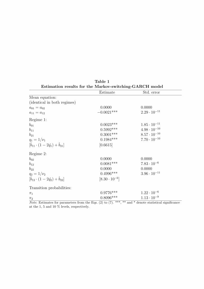
Table 1Estimation results for the Markov-switching-GARCH model
Estimate Std. errorMean equation:(identical in both regimes)a01 = a02 0.0000 0.0000a11 = a12 −0.0021*** 2.29 · 10−11
Regime 1:b01 0.0023*** 1.85 · 10−11
b11 0.5992*** 4.98 · 10−10
b21 0.3001*** 8.57 · 10−10
q1 = 1/ν1 0.1984*** 7.70 · 10−10
[b11 · (1− 2q1) + b21] [0.6615]
Regime 2:b02 0.0000 0.0000b12 0.0081*** 7.83 · 10−6
b22 0.0000 0.0000q2 = 1/ν2 0.4996*** 3.96 · 10−11
[b12 · (1− 2q2) + b22] [8.30 · 10−6]
Transition probabilities:π1 0.9776*** 1.22 · 10−6
π2 0.8096*** 1.13 · 10−9
Note: Estimates for parameters from the Eqs. (2) to (7). ***, ** and * denote statistical significanceat the 1, 5 and 10 % levels, respectively.


