economic analysis of high speed rail in europe · 2017. 6. 21. · economía y sociedad informes...

Economía y SociedadInformes 2009

Economía y Sociedad

Economic Analysis of H

igh Speed Rail in EuropeInform

es 2009

Ginés de Rus (Ed.)

Ignacio BarrónJavier Campos

Philippe GagnepainChris Nash

Andreu UliedRoger Vickerman

Plaza de San Nicolás, 448005 BilbaoEspañaTel.: + 34 94 487 52 52Fax: + 34 94 424 46 21

Paseo de Recoletos, 1028001 MadridEspañaTel.: +34 91 374 54 00Fax: +34 91 374 85 22

[email protected]

Economic Analysisof High Speed Railin Europe

Economic Analysis

of High Speed Rail in Europe

Economic Analysis

of High Speed Rail in Europe

Edited byGinés de Rus

Ignacio BarrónJavier CamposPhilippe GagnepainChris NashAndreu UliedRoger Vickerman

First published in May 2009

© the authors, 2009

© Fundación BBVA, 2009Plaza de San Nicolás, 4. 48005 [email protected]

A digital copy of this report can be downloaded free of charge at www.fbbva.es

The BBVA Foundation’s decision to publish this report does not imply anyresponsibility for its content, or for the inclusion therein of any supplementarydocuments or information facilitated by the authors.

Edition and production: Editorial Biblioteca Nueva, S. L.

ISBN: 978-84-96515-89-5Legal deposit no.: M-26.408-2009

Printed in Spain

Printed by Rógar, S. A.

This book is produced with 100% recycled paper made from recoveredfibres, in conformity with the environmental standards required by currentEuropean legislation.

AUTHORS ................................................................................................................ 9

ACKNOWLEDGEMENTS ........................................................................................... 11

SUMMARY – RESUMEN .......................................................................................... 13

INTRODUCTION ...................................................................................................... 15

1.A REVIEW OF HSR EXPERIENCES AROUND THE WORLD1.1. Introduction ................................................................................................ 191.2. Towards an economic definition of high speed railways ................................ 201.3. The costs of building HSR infrastructure ..................................................... 231.4. The costs of operating HSR services ............................................................ 26

1.4.1. Infrastructure operating costs ......................................................... 261.4.2. Rolling stock and train operating costs ............................................ 27

1.5. The external costs of HSR ........................................................................... 281.6. HSR demand: evolution and perspectives .................................................... 301.7. Conclusions ................................................................................................ 32

2.THE COST OF BUILDING AND OPERATING A NEW HIGH SPEED RAIL LINE2.1. Introduction ................................................................................................ 332.2. Project characteristics ................................................................................. 34

2.2.1. Overview and timeline .................................................................... 342.2.2. Operational characteristics .............................................................. 36

2.3. Demand and supply .................................................................................... 372.3.1. Demand estimation and distribution ................................................ 372.3.2. Supply parameters: train capacity and frequency ............................. 38

2.4. Methodology of cost calculations ................................................................. 422.4.1. Objectives ...................................................................................... 422.4.2. Infrastructure costs ........................................................................ 422.4.3. Rolling stock costs ......................................................................... 43

2.5. Conclusions ................................................................................................ 47

5

Contents

3.IN WHAT CIRCUMSTANCES IS INVESTMENT IN HSR WORTHWHILE?3.1. Introduction ................................................................................................ 513.2. Overview of costs and benefits .................................................................... 51

3.2.1. Options to consider ........................................................................ 513.2.2. Costs ............................................................................................. 523.2.3. Benefits ......................................................................................... 53

3.3. Empirical examples ..................................................................................... 553.3.1. British HSR proposals .................................................................... 553.3.2. The Spanish experience .................................................................. 57

3.4. Breakeven traffic volumes ........................................................................... 593.4.1. The model ...................................................................................... 593.4.2. Simplifying the model ..................................................................... 613.4.3. Demand thresholds for social profitability ........................................ 64

3.5. Conclusions ................................................................................................ 69

4.MEASURING THE INTERMODAL EFFECTS OF HIGH SPEED RAIL4.1. Introduction ................................................................................................ 714.2. Intermodal effects of HSR: a summary of empirical findings ........................ 72

4.2.1. The competitive advantage of HSR: the effect of travel time ............ 734.2.2. The competitive pressure of other modes: the effect of prices .......... 754.2.3. The growing role of HSR as a complement to other transport modes ..... 76

4.3. Explaining the intermodal effects of HSR: a theoretical approach ................. 774.3.1. Travellers’ modal choice .................................................................. 774.3.2. Transport operators’ profits ............................................................. 79

4.3.2.1. The primal cost function ................................................ 804.3.2.2. Competitive pressure and cost reduction ......................... 804.3.2.3. Optimal pricing .............................................................. 81

4.4. Implementing the model: a method to measure intermodal effects ............... 824.4.1. Cobb-Douglas technology ................................................................ 824.4.2. Estimation ..................................................................................... 834.4.3. The required data ........................................................................... 84

4.5. Simulation .................................................................................................. 844.6. Conclusions ................................................................................................ 87

5. INDIRECT AND WIDER ECONOMIC IMPACTS OF HIGH SPEED RAIL5.1. Introduction ................................................................................................ 895.2. The emerging European HSR network .......................................................... 905.3. Defining the wider effects of HSR ............................................................... 93

5.3.1. Accessibility ................................................................................... 935.3.2. Connectivity ................................................................................... 945.3.3. The impacts of accessibility change ................................................ 94

5.4. Economic impacts of HSR ........................................................................... 965.4.1. Defining wider economic benefits ................................................... 965.4.2. Imperfect competition and wider benefits ........................................ 975.4.3. Total economic impact .................................................................... 97

5.5. Evidence on the wider economic impacts of HSR ......................................... 995.6. National and local impacts of HSR .............................................................. 100

ECONOMIC ANALYSIS OF HIGH SPEED RAIL IN EUROPE

6

5.6.1. Some local impacts 1: evidence from the north European HSR network .......................................................................................... 101

5.6.2. Some local impacts 2: TGV South-west, the Spanish-French connection ..................................................................................... 103

5.7. Conclusions ................................................................................................ 103Appendix ............................................................................................................ 104

CONCLUSIONS ........................................................................................................ 119

REFERENCES .......................................................................................................... 121

LIST OF GRAPHS .................................................................................................... 127

LIST OF MAPS ......................................................................................................... 129

LIST OF TABLES ..................................................................................................... 131

CONTENTS

7

Editor:

Ginés de Rus. Professor of Applied Economics.Department of Applied Economics, University of Las Palmas of Gran Canaria, Spain

Contributors:

Ignacio Barrón. Director of High Speed. InternationalUnion of Railways (UIC), France

Javier Campos. Associate Professor. Department ofApplied Economics, University of Las Palmas of Gran Canaria, Spain

Philippe Gagnepain. Associate Professor.Department of Economics, University Carlos III of Madrid, Spain

Chris Nash. Professor of Transport Economics.Institute for Transport Studies, University of Leeds,UK

Andreu Ulied. Director MCRIT. Barcelona, Spain

Roger Vickerman. Professor of European Economics.Department of Economics, University of Kent,Canterbury, UK

9

Authors

As editor of this report, I must say that it has beenan honor to coordinate such an excellent researchteam. Each one of its members agreed to partici-pate in the project without previous conditions:Chris Nash, Roger Vickerman, Iñaki Barrón,Philippe Gagnepain, Andreu Ulied, and JavierCampos. Their research capacity and their posi-tive, constructive, and generous attitude made itan enriching and stimulating experience. I am

also in debt to Jorge Valido and Beatriz Ojeda fortheir assistance. We gratefully acknowledge thefinancial support of the BBVA Foundation, andespecially its effort to keep administrative coststo a minimum, creating the adequate conditionsfor research.

GINÉS DE RUS

Tafira, September 2008

11

Acknowledgements

Many countries are taking into consideration theconstruction of new high speed rail lines. The Eu-ropean Commission explicitly deems the expan-sion of high speed rail as a priority within thetrans-European networks, allocating an importantpart of the community funds for its developmentwith the declared aim of increasing the marketshare of rail transport.

High speed rail generates social benefits, whichstem from time savings, increase in reliability,comfort and safety, as well as from the reductionof congestion and accidents in alternative modes.Another benefit of investing in the constructionof new lines is the capacity released in the con-ventional network, when the latter itself can beused for freight transport.

The question is not whether users and other pos-sible beneficiaries of high speed rail would votein favor of constructing a new line. The questionis whether they would be willing to pay (regard -less of what they actually pay) for its socialcosts. The answer to this question varies widelydepending on the particular characteristics of the

project. An exhaustive review of the economic li-terature shows that the research effort dedicat edto the economic analysis of investing in high spe-ed railways is insignificant when compared withthe economic importance of such technol ogy andits public financing within the transport plansand budgets of member states and the EuropeanCommission.

The aim of this report is to contribute to theeconomic analysis of new high speed rail invest -ment projects requiring public funds. The eco-nomic evaluation of projects can help govern-ments to obtain a clearer view of the expectednet benefits of different lines of action, as it at-tempts to identify the projects which reallydeserve the sacrifice of other social needs com-peting for the same public funds. We analyzethe circumstances under which society may ben -efit from investing in high speed rail, andwhen it is sensible to delay the investment de-cision. The high speed rail network may bebuilt gradually, adding new lines once the eco-nomic evaluation of projects shows a positivesocial profitability.

La construcción de líneas ferroviarias de alta ve-locidad es una opción que está siendo considera-da por muchos países en el mundo. La ComisiónEuropea considera que la expansión de la red dealta velocidad es una prioridad dentro de las re-des transeuropeas, destinando una importantecantidad de fondos comunitarios para su desarro-llo con el objetivo explícito de aumentar la cuotade mercado del ferrocarril.

La alta velocidad genera beneficios sociales pro-cedentes de ahorros de tiempo, mejoras en la fia-bilidad, confort y seguridad del servicio de trans-porte; y de la reducción de la congestión y losaccidentes en los modos alternativos de transporte.Liberar capacidad en la red convencional, quepuede utilizarse para el transporte de mercancías,es también un beneficio adicional de la inversiónen la construcción de nuevas líneas.

13

Summary

Resumen

La cuestión no es si los usuarios y otros potencia-les beneficiarios votarían a favor de la construc-ción de nuevas líneas de alta velocidad. La cues-tión relevante es si estarían dispuestos a pagar(con independencia de lo que paguen) los costessociales de su puesta en funcionamiento. La res-puesta a esta pregunta varía ampliamente depen-diendo de las circunstancias concretas del pro-yecto. Una exhaustiva revisión de la literaturaeconómica muestra que el análisis económico delas inversiones en alta velocidad es insignifican-te comparado con el papel concedido a esta tec-nología dentro de los planes de transporte de mu-chos países miembros y de la propia ComisiónEuropea, y más aún si tenemos en cuenta la fi-nanciación pública destinada a los mismos.

Este informe pretende contribuir al análisiseconómico de los proyectos de inversión en altavelocidad ferroviaria. La evaluación económicade proyectos puede ayudar a los gobiernos aformarse una idea más precisa sobre los bene-ficios esperados de distintas líneas de actua-ción que absorben dinero público para resolverun mismo problema de transporte. En este in-forme tratamos de determinar las circunstan-cias en las que la inversión en alta velocidad essocialmente deseable y en que otras la socie-dad gana posponiendo la inversión. La red dealta velocidad puede construirse gradualmente,añadiendo nuevas líneas una vez que la evalua-ción económica muestra una rentabilidad so-cial positiva.


14

The allocation of public resources to the expan-sion of the high speed rail network is a signifi-cant element of transport policy in many coun-tries all over the world. This includes both theconstruction of new lines and the upgrading ofpart of the conventional network, so that trainscan run at speeds of more than 200 km per hour.The demand for the new rail transport alternativecomes from deviated traffic from conventionaltrains, air and road transport, and also from gen-erated traffic, thanks to the combination of timesavings, increased comfort and more price choic-es associated to this new transport option.

The European Union has explicitly consideredthe expansion of high speed rail as a prioritywithin the trans-European networks, assigning animportant part of Community funds for its devel-opment, with the declared aim of changing themodal split to the benefit of railways. This revi-talization of railways strategy, as announced bythe European Commission, reflects the relevancethat this transport mode is gaining in Europe in acontext of increased worries about congestionand traffic accidents in roads, the delays and dis-comfort associated with air traffic, as well as thenegative environmental impacts of these modes.

Although the construction and operation of highspeed rail lines imply significant environmentalcosts (land, noise, barrier effects, visual intru-sion and global warming) the train still retains agood environmental image, though the actual en-vironmental balance depends on the volume oftraffic and its composition.

The interest of the European Commission in highspeed rail is shared by most member state gov-

ernments, and, obviously, by the industrial lobbiesthat supply rolling stock and other rail inputs, aswell as by users, who generally enjoy its speed,comfort and price—three elements responsiblefor the dramatic recovery of the railway’s marketshare over medium distances.

If users, governments, industries and the Euro-pean Commission support such a technological op-tion for passenger travel, we could be in a situationthat economists call Paretian improvement, char-acterized by the existence of winners, indifferentagents and the inexistence of losers. Neverthe-less, the price that users pay for high speed railinfrastructure and services in many routes is farfrom covering construction, maintenance and in-frastructure operation costs. That means taxpay-ers must contribute financially to the support ofthese projects. So there are in fact losers, as inall public policies and investment projects.

The question is not whether users and other pos-sible beneficiaries of high speed rail would votein favor of the construction of high speed lines.The question is whether they would be willing topay (independently of what they actually pay)their social costs. The answer to this questionvaries widely depending on the local characteris-tics of the project: routes, crossed urban zones,required bridges and tunnels, volume of demand,per capita income, and the level of capacity usein competing modes.

Social benefits of high speed rail mainly accruefrom users’ time savings and the willingness topay of generated traffic. To these benefits weshould add those that users experience thanks tothe reduction of congestion and accidents in al-

15

Introduction

ternative modes. The benefits obtained from therelease of capacity in the conventional networkshould also be added.

The conventional economic evaluation of projectsrequires the identification of the benefits andcosts during the life of the project. And once thesehave been quantified, the next step is to calculatetheir net value. When benefits are higher thancosts, the investment is probably socially worthy,although even with a positive net present value,there may be other alternative projects providing ahigher social benefit.

What happens when the flow of expected netbenefits is lower than the investment costs of theproject under evaluation? Or, in more intuitiveterms: what happens when the society is willingto pay a price for a high speed rail line which isinferior to its cost? The answer is clear: reject theproject.

In the debate in favor of large infrastructure in-vestment projects, there is a recurrent argumentwhich defends the existence of economic bene-fits greater than those described above. It alsosuggests that the exclusion of these unaccountedbenefits would make the high speed rail line ap-pear less profitable than it really is. The identifi-cation and magnitude of these wider economicbenefits are difficult to determine, and it maywell be that, due to this fact, promoters andpoliticians who support high speed lines mentionthem frequently when debating the convenienceof building new lines.

The indirect economic benefits are located inmarkets other than those directly affected by theproject, or the primary markets. No one doubtsthe existence of secondary effects. A city that isconnected to a high speed network may expe -rience an economic expansion and an increase inits land value. Unemployment may be reduced asa consequence of the activity generated thanks tothe construction of the rail line and the genera-tion of economic activity.

However there are also some other effects to ac-count for. Someone has to pay for the higherprice of the land; and although there are net ben-efits, the analyst has to be careful not to count

pure rent transfers as net benefits, or to see theincrease in land value as something additional totime savings and other primary benefits. Regard-ing employment, we ought not to confuse inputswith outputs. If there is unemployment, the priceof labor will be reduced in the evaluation to re-flect its opportunity cost. Adding it again on thebenefit side would lead to double counting.

Before adding the secondary benefits, it is impor-tant to distinguish the creation of a new activityfrom one that emerges from a simple relocationof an already existing economic activity. In gen-eral, the analysis of indirect economic effects ismore complicated than it may seem at firstglance. Moreover not all of them are positivewhile many others reflect already accounted-forbenefits of the primary market.

Even assuming that all the benefits of high speedrail were adequately measured and compared to itscosts, promoters will frequently argue that theselarge infrastructure initiatives (mega-projects) willhave more important, long-term effects on societythan direct economic benefits. Although very dif-ficult to predict, these effects are usually relatedto the regional development benefits of investingin infrastructure. Nevertheless, thanks to the ef-forts of new economic geography researchers, weknow that the effects of infrastructure on the lo-cation of economic activity are ambiguous attimes: occasionally reinforcing the central regionand making the periphery worse off.

Investment in building HSR lines and the associ-ated rolling stock to operate them is very expen-sive, and their indivisibility and irreversibility in-crease the cost of errors. Constructing new lineswith an optimistic demand bias translates into awaste of taxpayer money, because this mode oftransport is being developed in Europe within thepublic sector, without private participation andwith revenues far from covering total costs.

What do economists say about the opportunity ofinvesting in high speed networks in Europe? Anexhaustive revision of the specific economic liter -ature shows that the research effort devoted tothe economic analysis of investing in high speedrailways is almost insignificant considering theeconomic significance of this technology within


16

the transport plans of member states and the Eu-ropean Commission, and its share in the statebudgets of many countries.

The aim of this report is to contribute to the eco-nomic analysis of new high speed rail investmentprojects that are waiting for public funds. Theeconomic evaluation of projects can help govern-ments to obtain a clearer view of the expectednet benefits of different lines of action, and iden-tify the projects which really deserve the sacri -fice of other social needs competing for the samepublic funds.

Constructing a new high speed rail line may re-duce congestion and accidents in road and airtransport over medium distances, where the traincompetes with the private vehicle and the air-lines. If the volume of demand is high enough,the project may be socially profitable. In addi-tion, when a high speed line is linked to a net-work, it multiplies its connectivity, making neworigins and destinations accessible. This factorand the release of capacity in the conventionalrail network or in congested airports increase theprobability of a positive net present value.

Deciding to reject (or delay) the construction of ahigh speed rail line is not necessarily a positionagainst progress. If the best information avail-able ex ante proves that there are other transportoptions with a higher net social benefit, the mostappropriate decision is to select such optionsand not the larger, more costly or newest technol-ogy.

The social pressure for the construction of highspeed lines is not only explained by its knownbenefits but also by an institutional design thatfavors the construction of projects without havingto pay for them directly. Incentives today lean to-wards the approval of mega-projects, which acountry or a region, without supranational orstate funds respectively, would not have under-taken on its own.

The research papers published in this report be-gin with the construction of a database from in-complete and disperse information on high speedlines all over the world. The report contains ananalysis of the construction costs, maintenance,and exploitation of the lines in service or underconstruction, and it examines the demand dataavailable. The economic evaluation of investmentin high speed rail under different circumstanceshows the conditions required for a minimum lev-el of social profitability.

The texts included here have a common feature,which is the attempt to answer the question thatmotivated this research project: when is the in-vestment in high speed rail profitable from a so-cial perspective? The answer, as in so many as-pects of economy, is not black and white. Itdepends on the local conditions where the newline is to be built and the expected volume of de-mand. Choosing an investment option withoutcomparing it with relevant alternatives is, at best,contrary to good economic practice. The primaryfunction of high speed railways is to solve atransport problem, and their advantage over oth-er feasible alternatives has to be demonstratedon a case-by-case basis.

INTRODUCTION

17

1 Although the definition of HSR services will be discussedin section 1.2, the list includes Japan, South Korea,China, Taiwan, France, Germany, Italy, Spain, Portugal,

Belgium, Netherlands, Norway, United Kingdom, Swe-den, Denmark, and the United States.

1.1 INTRODUCTION

High Speed Railways (HSR) is currently regardedas one of the most significant technologicalbreakthroughs in passenger transportation devel-oped in the second half of the 20th century. Atthe beginning of 2008, there were about 10,000kilometers of new high speed lines in operationaround the world and, in total (including upgrad-ed conventional tracks), more than 20,000 kilo-meters of the worldwide rail network was devotedto providing high speed services to passengerswilling to pay for lower travel time and quality im-provement in rail transport.

For the last 40 years in Japan alone, where theconcept of bullet train was born in 1964, 100million passenger-trips are carried out per year. InEurope, traffic figures average 50 million passen-ger-trips per year, although they have been steadi-ly growing since 1981 by an annual percentagerate of 2.6. Nowadays, there are high speed railservices in more than 15 countries,1 and the net-work is still growing at a very fast pace in manyothers: it is expected to reach 25,000 kilometersof new lines by 2020 (UIC 2005a).

However building, maintaining and operating HSRlines is expensive; it involves a significant amountof sunk costs and may substantially compromiseboth the transport policy of a country and the de-velopment of its transport sector for decades. Forthese reasons, it deserves a closer look, well be-

yond the technological hype and the demand fig-ures. The main objective of this chapter is to dis-cuss some characteristics of the HSR services froman economic viewpoint, while simultaneously de-veloping an empirical framework that should helpus to understand, in more detail, the cost and de-mand sides of this transport alternative. This un-derstanding is especially useful for future projects,since it will lead to a better analysis of the expect-ed construction and operating costs, and of thenumber of passengers to be transported under dif-ferent economic and geographic conditions.

Such understanding is particularly relevant be-cause the economic magnitude of HSR invest-ments and the described prospects for networkexpansion are not in accordance with the researchefforts reported in the economic literature. Theeconomic appraisal of particular corridors is lim-ited to some existing and projected lines (see DeRus and Inglada 1993, 1997; Levinson et al.1997; Atkins 2003; Coto-Millan and Inglada2004; and De Rus and Roman 2005). General as-sessments are relatively scarce (Nash 1991; Vick-erman 1997; Martin 1997; SDG 2004; De Rusand Nombela 2007; and De Rus y Nash, 2007);and many other papers were devoted to assess theregional and other indirect effects of HSR (Bon-nafous 1987; Vickerman 1995; Blum, Haynesand Karlsson 1997; Plassard 1994, Haynes1997, and Preston and Wall 2007).

Since most of the previous empirical assess-ments were based on individual country case

19

1

A Review of HSR Experiences

Around the World

2 The analysis carried out in this chapter and, in particu-lar, the list of HSR projects are based on public infor-mation mainly provided by the International Union ofRailways (see UIC 2006), and some of the rail compa-nies currently operating HSR services.

3 Information on the demand side (disaggregated trafficfigures and prices) is still incomplete and constitutesthe major drawback of our dataset.

4 The only comparable database built with a similar pur-pose is The World Bank Railway Database (available at

www.worldbank.org/transport/rail/rdb.htm). However ourdata specifically focus on HSR projects, not on the over-all performance of rail operators worldwide.

5 This Directive aims to ease the circulation of high speedtrains through the various train networks of the EuropeanUnion. Member States are asked to harmonize their highspeed rail systems in order to create an interoperable Eu-ropean network (European Commission 1996).

6 The average commercial speed in several (supposedly)high speed services over the densest areas in North Eu-

studies, we will adopt an international compara-tive perspective. We assembled a database com-prising all existing HSR projects around theworld at the beginning of 2006.2 It includes in-formation about the technical characteristicsand building costs of each project—even forthose still at planning or construction stage,when available—plus detailed information re-garding operating and maintenance costs of in-frastructure and services for the lines already inoperation. A special section devoted to the exter-nal costs of HSR is included, as well as data re-garding traffic, capacity and tariffs on selectedcorridors.3

Our database includes information on 166 proj-ects in 20 countries; 40 (24%) are projects al-ready in operation, whereas 41 are currently un-der construction and 85 are still at planningstage, some of which pending further approvaland/or funding. The projects in operation andconstruction have a total length of 16,400 kilo-meters, although some of them will not be fin-ished before 2015.4

The statistical analysis and data comparisons ob-tained from such a large number of projects willallow us to address several questions about HSRaround the world. The first one (section 1.2) isrelated to the economic definition of HSR. Insection 1.3, we try to find out (on average) thecost of building a kilometer of (new) high speedline, and to identify the reasons why this cost dif-fers across projects. Section 1.4 is devoted to ex-tract, from actual data, some of the main charac-teristics of operating and maintenance costs ofHSR lines in the world, whereas in section 1.5,we discuss the extended idea of HSR being themeans of transport with the lowest external cost.Section 1.6 studies how the demand path forhigh speed services evolves around the world,

and it tries to look for a pattern to predict howlong it will keep on growing in Europe at the pres-ent rate. Finally, section 1.7 contains the gener-al conclusions.

1.2 TOWARDS AN ECONOMIC DEFINITION

OF HIGH SPEED RAILWAYS

For many years it has been customary in the railindustry to consider high speed just as a techni-cal concept related to the maximum speed trainscould reach when running on particular tracksegments. In fact, the European Council Direc-tive 96/48 specifically established that highspeed infrastructure comprised three differenttypes of lines:5

— purposely built high speed lines equipped forspeeds generally equal to or greater than 250km/h,

— upgraded conventional lines, equipped forspeeds of the order of 200 km/h, and

— other upgraded conventional lines, which havespecial features as a result of topographical orland-planning constraints, on which the speedmust be adapted to each case.

In theory, these technical definitions are broadenough to encompass the entire rail infrastruc-ture capable of providing high speed services. Inpractice, however, speed has not always been thebest indicator, since commercial speed in manyservices is often limited due to, for example,proximity to densely urbanized areas (to ease theimpact of noise and minimize the risk of acci-dents), or the existence of viaducts or tunnels(where speed must be reduced to 160-180 km/hfor safety reasons).6


20

rope is often below the average speed of some conven-tional lines, running between distant stops throughsparsely populated plain areas. New maximum speedtests have been recently (2007) announced by the TGVin France (www.sncf.com/news), but its commercial usemay be restricted.

7 In recent years a new technology, based on magnetic levi-

tation (maglev) trains that can reach up to 500 km/h,has been implemented in a limited number of projects(e.g. Shanghai). In spite of sharing the adjective highspeed, the services provided by these trains are basedon completely different principles—closer to air trans-port than to railways—and will not be considered in thischapter.

Although HSR shares the same basic engineeringprinciples with conventional railways—both arebased on the fact that rails provide a very smoothand hard surface on which the wheels of thetrains may roll with a minimum of friction andenergy consumption—they also have technicaldifferences. For example, from an operationalpoint of view, their signalling systems are com-pletely different: whereas traffic on conventionaltracks is still controlled by external (electronic)signals together with automated signalling sys-tems, the communication between a runningHSR train and the different blocks of tracks isusually fully in-cab integrated, which eliminatesthe need for drivers to see lineside signals.

Similarly, the electrification differ: whereas mostnew high speed lines require at least 25,000volts to achieve enough power, conventional linesmay operate at lower voltages. Additional techni-cal dissimilarities, regarding the characteristicsof the rolling stock and the exploitation of servic-es, also exist.7

All these differences suggest that, more than thespeed factor, what actually plays a more relevantrole in the economic definition of high speedservices are both the relationship of HSR with ex-isting conventional services, and the way inwhich the use of infrastructure is organized. Assummarized in graph 1.1, four different exploita-tion models can be identified:

1) The exclusive exploitation model is character-ized by a complete separation between highspeed and conventional services, each one withits own infrastructure. This is the model theJapanese Shinkansen has been adopting since1964, mostly due to the fact that the existingconventional lines (built in narrow gauge, 1.067m) had reached their capacity limits, and it wasdecided that the new high speed lines would bedesigned and built in standard gauge (1.435 m).One of the major advantages of this model is thatmarket organization of both HSR and convention-al services are fully independent, something thatlater proved to be a valuable asset, when thepublic operator (Japan National Railways, JNR)

A REVIEW OF HSR EXPERIENCES AROUND THE WORLD

21

Graph 1.1 HSR models according to the relationship with conventional services

High Speed Tracks Conventional Tracks

High Speed Trains Conventional Trains

Model 1: Exclusive exploitation



Model 3: Mixed conventional

Model 2: Mixed high speed

Model 4: Fully mixed





8 There are a few exceptions. Some Shinkansen lines can-not handle the highest speeds. This is because somerails remain narrow gauge to allow sharing with conven-tional trains, reducing land requirement and cost. In ad-dition, in the congested surroundings of Tokyo and Osa-ka, the Shinkansen must slow down to allow other trainsto keep their schedules and must wait for slower trainsuntil they can be overtaken (Hood, 2006).

9 The wheels in TALGO trains are mounted in pairs

between, rather than underneath, the individual coach-es. They are not joined by an axle and, thus, the trainscan lightly switch between different gauge tracks.

10 Note that for each intermediate stop, the dotted lineswould jump to the right for a distance proportional tothe time spent at the stop. In multiple track lines or instations with multiple platforms, faster trains could over-take slower ones.

went bankrupt, and integrated rail services andinfrastructures had to be privatized.8

2) In the mixed high speed model, high speedtrains run either on specifically built new lines oron upgraded segments of conventional lines. Thiscorresponds to the French model, whose TGV(Train à Grande Vitesse) has been operating since1981, mostly on new tracks, but also on re-elec-trified tracks of conventional lines in areas wherethe duplication was impractical. This reducesbuilding costs, which is one of the main advan-tages of this model.

3) The mixed conventional model, where someconventional trains run on high speed lines, wasadopted by Spain’s AVE (Alta Velocidad Españo-la). As in Japan, most of the Spanish conven-tional network was built in narrow gauge, where-as the rest of the European network used thestandard gauge. To facilitate the interoperabilityof international services, a specific adaptivetechnology for rolling stock was developed in1942—i.e., the TALGO trains—to enable it touse, at higher than normal speed, the specificHSR infrastructure (built in standard gauge).9

The main advantages of this model are the sav-ing of rolling stock acquisition and maintenancecosts, and the flexibility for providing intermedi-ate high speed services on certain routes.

4) Finally the fully mixed model allows for themaximum flexibility, since this is the case whereboth high speed and conventional services canrun (at their corresponding speeds) on each typeof infrastructure. This is the case of German in-tercity trains (ICE) and the Rome-Florence line inItaly, where high speed trains occasionally useupgraded conventional lines, and freight servicesuse the spare capacity of high speed lines duringthe night. The price for this wider use of the in-

frastructure is the significant increase in mainte-nance costs.

The reasons why each of these models will deter-mine in a different way the provision of HSR serv-ices depend on traffic management restrictions,which can be better understood with the help ofgraph 1.2.

On the vertical axis, we have represented the dis-tance (250 km) between origin (O) and destina-tion (D) rail stations, whereas the horizontal axisreflects the travel time (in hours). The inclineddotted lines represent potential time slots for(non-stop) trains running from O to D.10 Note thatthe slope of the slots and the horizontal separa-tion between each pair of them depend on the av-erage commercial speed authorized for the O-Dline (according to its technical configuration,gradient, number of curves, viaducts, etc.) How-ever, the actual usage of these slots is mainly de-termined by the type of service provided to pas-sengers. For example, high speed services (at250 km/h) cover the distance between O and Din just one hour, whereas a conventional trainwould need 2.5 hours.


22

Graph 1.2 Time slots in railways and the provision of HSRservices

Distance

(km)

Travel time (h)

250

km

D

HS tr

ain

1HS

trai

n 2

HS tr

ain

3HS

trai

n 4

OCon

ventio

nal train

0 0.5 1.0 1.5 2.52.0

For this reason the network exploitation modelsin graph 1.1 now become crucial. The exclusiveexploitation and the mixed high speed models,for example, allow a more intensive usage of HSRinfrastructure, whereas the other models musttake into account that (with the exception of mul-tiple-track sections of the line) slower trains oc-cupy a larger number of slots during more timeand reduce the possibilities for providing HSRservices. In graph 1.2, at least four high speedtrains are stopped due to the operation of a sin-gle conventional train. Since trains of significant-ly different speeds cause massive decreases ofline capacity, mixed-traffic lines are usually re-served for high speed passenger trains duringdaytime, while freight trains operate at night. Insome cases, nighttime high speed trains are evendiverted to lower speed lines in favor of freighttraffic.

Since choosing a particular exploitation model isa decision affected by the comparison of thecosts of building (and maintaining) new infra-structure versus the costs of upgrading (andmaintaining) the conventional network, the defi-nition of HSR immediately becomes not only atechnical question but also a (very relevant) eco-nomic one. Three additional factors contribute tothe definition of HSR in economic terms:

— The first one is the specificity of the rollingstock, whose technical characteristics must beadapted to the special features of high speed.HSR trainsets are designed to run without lo-comotives (both extremes of a train can func-tion as the initial one), with minimal oscilla-tions even on curves with elevated radialvelocity, and without the need of tilting tocompensate for the centrifugal push. The ac-quisition, operating and maintenance costs ofthis rolling stock represent a huge long-run in-vestment for companies (often over 20 years),and critically determine the provision of highspeed services.

— The second one is the public support enjoyedby most HSR undertakings, particularly in Eu-rope where national governments have alreadycompromised significant amounts of funds inthe development of their high speed networksduring the next decades. At the supranationallevel (European Commission 2001) there ex-

ists an explicit strategy for «revitalizing therailways» as a «means for shifting the balancebetween modes of transport against the cur-rent dominance of the road». This is justifiedin terms of the lower external costs of railtransport (particularly, HSR) when comparedto road transport with respect to congestion,safety, and pollution.

— The third reason lies on the demand side forHSR services. Railways operators in many coun-tries have widely acknowledged their highspeed divisions as one of the key factors in thesurvival of their passenger rail services. In fact,HSR has been started to be publicized—partic-ularly in France and Spain—as a different modeof transport, as a system with its own right thatencompasses both a dedicated infrastructurewith an increasingly more specialized and tech-nologically advanced rolling stock. It bringswith it an improvement over traditional railtransport (clock-face timetables, sophisticatedinformation and reservation systems, catering,on board and station information technologyservices) and, in general, an overall increase inthe added value for the passenger.

All these elements—infrastructure building costs,operating and maintenance costs, external costsand demand—will be analyzed in the remainingsections of this chapter.

1.3 THE COSTS OF BUILDING HSR

INFRASTRUCTURE

Building new HSR infrastructure requires a spe-cific design aimed at the elimination of all thosetechnical restrictions that may limit the commer-cial speed below 250-300 km/h. These basicallyinclude roadway level crossings, frequent stopsor sharp curves unfitted for higher speeds; how-ever, in some cases, new signalling mechanismsand more powerful electrification systems may beneeded, as well as junctions and exclusive track-ways in order not to share the right-of-way withfreight or slower passenger trains, when the infra-structure is jointly exploited (see the models ingraph 1.1).

Such common design features, however, are notan indication of similarly in HSR construction.


23

11 In most projects the superstructure costs often includebuilding standard stations and auxiliary depots whichalone, according to their architectonic characteristicscannot be considered singular projects. In some cases,stations are singular buildings with an architectonic de-sign and associated costs far beyond the mini-

mum required for operating purposes. The allocation ofthese costs to the HSR line is arbitrary to say the least.There also are other minor elements (supervision, qual-ity control, etc.) in each project that may represent be-tween 1-5% of the total investment.

Just the opposite; the comparison of constructioncosts between different HSR projects is difficultsince each technical solution to implement thesefeatures not only differs widely (depending on to-pography and geography), but also evolves over-time.

According to UIC (2005b), building new HSR in-frastructure involves three major types of costs:

— Planning and land costs, including feasibilitystudies (both technical and economic), tech-nical design, land acquisition and other costs(such as legal and administrative fees, licens-es, permits, etc.) These costs may be substan-tial in some projects (particularly, when costlyland expropriations are needed), but they of-ten represent a sunk component of between 5-10% of the total investment amount.

— Infrastructure building costs including allthose costs related to terrain preparation andplatform building. The amount varies widelyacross projects depending on the characteris-tics of the terrain, but usually represents be-tween 10-25% of the total investment in newrail infrastructure. In some cases, the need ofsingular solutions (such as viaducts, bridges ortunnels) to geographic obstacles may easilydouble this amount (up to 40-50%, in moretechnically difficult projects).

— Superstructure costs include rail specific ele-ments such as guideways (tracks) and sidingsalong the line, signalling systems, catenariesand electrification mechanisms, communica-tions and safety installations, etc. Individuallyconsidered, each of these elements usuallyrepresents between 5-10% of the total invest-ment.11

Although these three major types of costs arepresent in all projects, their variability is largelyconditioned again by the relationship betweenthe infrastructures to be built in each case andthe pre-existing one. Attending to this criterion,

at least five types of HSR projects can be distin-guished (UIC, 2005b):

— Large corridors isolated from other HS lines,such as the Madrid-Seville AVE;

— Network integrated large corridors, such asParis-Lille integrated with Paris-Lyon and theFrench high speed network;

— Smaller extensions or complements of existingcorridors, such as Madrid-Toledo or Lyon-Va-lence, both developed to serve nearby medi-um-size cities;

— Large singular projects, such as the Eurotun-nel, the Grand Belt or the bridge over theMessina Strait; and

— Smaller projects complementing the conven-tional network, including high speed lines thatconnect airport with nearby cities, or the im-provements in conventional infrastructure toaccommodate higher speed services, as inGermany or Italy.

Our database of 166 HSR projects around theworld includes information about all these fivetypes of projects. However, in the comparison ofbuilding costs, we only considered 45 projects.We excluded both the large singular projectsand the smaller projects complementing theconventional network, due to their specific con-struction characteristics. Projects whose finan-cial information was incomplete and all thosethat are still at planning stage, even when in-vestment information was available, were ex-cluded. The reason for the latter exclusion isthat, at such stage, deviation over plannedcosts is often substantial, as pointed out in theliterature about it (see Flyvbjerg, Skamris, andBuhl 2004, for example).

Graph 1.3 summarizes the average cost per kilo-meter of building HSR infrastructure found inour database. The values are expressed in euromillion (2005) and include the infrastructureand superstructure costs, but not the planning


24

12 This is qualitatively consistent with the comparison per-formed by SDG (2004), although the costs included inUIC (2005b) are different. Several individual projectsreported in SDG (2004)—such as the HSL Zuid (Nether-lands) and the Channel Tunnel rail link—have construc-tion costs per km in the range of €50-70 million.

13 The only exception in graph 1.3 is Italy. This is becausethe lines under construction are mostly placed in thenorth of the country, more densely populated.

and land costs. Overall, the construction costper kilometer in the sample of 45 projects variesbetween 6 and 45 million (with an average val-ue of 17.5 million). When the analysis is re-stricted to projects in operation (24 projects) therange varies between 9 and 39 million (with amean value of 18 million). With the exception ofChina, building HSR in Asia seems more expen-sive than in Europe, according to the data fromJapan, Taiwan and South Korea, although thecosts of these two latter countries include someitems corresponding to upgrading conventionaltracks.12

In Europe, there are two groups of countries:France and Spain have slightly lower buildingcosts than Germany, Italy and Belgium. This isexplained not only by the similar geography andexistence of the less populated areas outside themajor urban centers, but also by constructionprocedures. In France, for example, the cost ofconstruction is minimized by adopting steepergrades rather than building tunnels and viaducts.Because the TGV lines are dedicated to passen-gers (the exclusive exploitation model of graph1.1), grades of 3.5%, rather than the previousmaximum of 1-1.5% for mixed traffic, are used.Although the land acquired to build straighter

lines is more expensive, this is compensated by areduction in line construction as well as operat-ing and maintenance costs. In the other Euro-pean countries high speed rail is more expensivebecause it is built over more densely populatedareas, without those economies of space.

Finally, with respect to the projects currentlyunder construction (21 projects, some of themdue to finish by 2007), one can observe that,in most cases, they are in line with the build-ing costs of projects in operation.13 It is inter-esting to note that there is no evidence ofeconomies of experience, particularly in Japanand France, the countries with a longer historyof HSR projects, though the new projects arenot homogeneous enough to make relevantcomparisons.

In Japan, the cost per kilometer (excluding landcosts) in the Tokyo-Osaka Shinkansen (started in1964) was relatively low (€5.4 million in 2005values), but in all the projects carried out duringthe following years, this figure was tripled orquadrupled. In France, each kilometer built forthe TGV Sud-Est between Paris and Lyon, inau-gurated in 1981, required an investment of€4.7 million (in construction costs), whereas the


25

Graph 1.3 Average cost per kilometer of newHSR infrastructure

Notes: S = Lines in Service; C= Lines under Construc-tion (2006)

Source: HSR Database. Elaborated from UIC (2005b).Data excludes planning and land costs

25.5

80

60

40

20

0

Euro

(in

mill

ions

, 200

5)

Austria

S C S C S C S C S C S C S C S C S C S C

Belgium France Germany Italy Japan Korea Netherlands Spain Taiwan

39.6

18.5

16.115.0

18.8

4.7

23.0

10.015.0

28.8

33.0

21.0

14.0

65.8

20.0

30.9

40.0

25.0

34.2

43.7

7.8

20.0

17.5

8.9

39,5

14 This section deals only with the private costs faced bythe infrastructure management agencies and HSR oper-ators. Section 1.5 is devoted to the discussion of someof the external costs associated with HSR.

15 In countries where infrastructure is separately managed, ac-cess charges may represent an additional operating cost foroperators, but they are mere transfer of funds, when consi -dered from the perspective of the HSR system as a whole.

For an analysis of the different options to introduce compe-tition through vertical unbundling while maintaining verticalintegration, see Gómez-Ibáñez and De Rus (2006).

16 Note, however, that data comparability may be limitedby other technical factors, very difficult to homogenize,such as required reliability index, the inspection inter-vals, track geometry, average load, etc., which may dif-fer across countries and specific lines.

cost per kilometer of the TGV Méditerranée, in-augurated in 2001 was €12.9 million. Thesedifferences—due to intrinsic characteristics ofeach project—call once more for a cautious useof the comparison figures obtained in this andother papers.

1.4 THE COSTS OF OPERATING HSR

SERVICES

Once the infrastructure is built, the operation ofHSR services involves two types of costs: those re-lated to the exploitation and maintenance of theinfrastructure itself, and those related to the pro-vision of transport services using that infrastruc-ture. The different degrees of vertical integrationexisting between the infrastructure provider andthe carrier that supplies HSR services are not dis-cussed here.14 In Europe, Council Directive91/440 set out the objective of unbundling infra-structure from operations by either full separationor, at least, the creation of different organizationsor units (with separate accounts) within a holdingcompany. Outside Europe, many countries havestill opted for the full vertical integration model,where all the HSR operating costs are controlledand managed by a single entity.15

1.4.1 INFRASTRUCTURE OPERATING COSTS

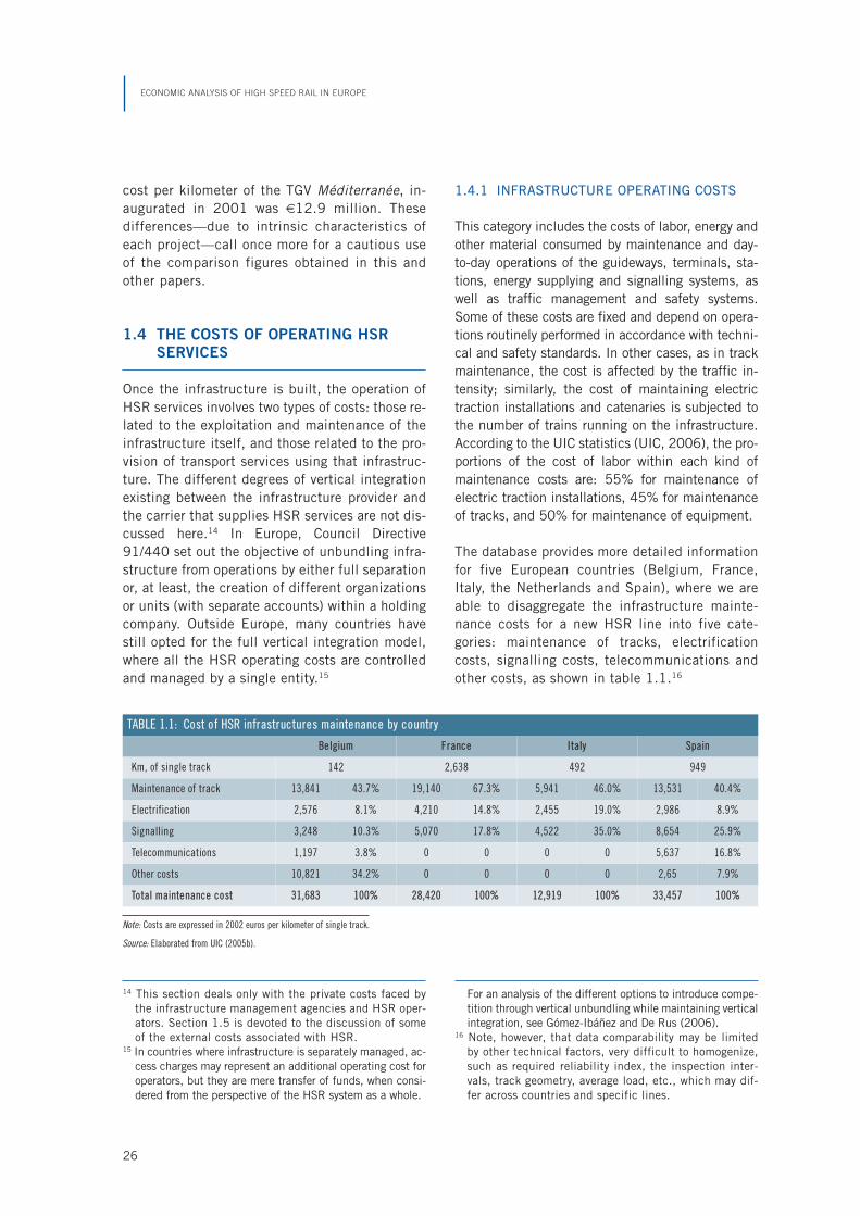
This category includes the costs of labor, energy andother material consumed by maintenance and day-to-day operations of the guideways, terminals, sta-tions, energy supplying and signalling systems, aswell as traffic management and safety systems.Some of these costs are fixed and depend on opera-tions routinely performed in accordance with techni-cal and safety standards. In other cases, as in trackmaintenance, the cost is affected by the traffic in-tensity; similarly, the cost of maintaining electrictraction installations and catenaries is subjected tothe number of trains running on the infrastructure.According to the UIC statistics (UIC, 2006), the pro-portions of the cost of labor within each kind ofmaintenance costs are: 55% for maintenance ofelectric traction installations, 45% for maintenanceof tracks, and 50% for maintenance of equipment.

The database provides more detailed informationfor five European countries (Belgium, France,Italy, the Netherlands and Spain), where we areable to disaggregate the infrastructure mainte-nance costs for a new HSR line into five cate-gories: maintenance of tracks, electrificationcosts, signalling costs, telecommunications andother costs, as shown in table 1.1.16


26

TABLE 1.1: Cost of HSR infrastructures maintenance by country

Belgium France Italy Spain

Km, of single track 142 2,638 492 949

Maintenance of track 13,841 43.7% 19,140 67.3% 5,941 46.0% 13,531 40.4%

Electrification 2,576 8.1% 4,210 14.8% 2,455 19.0% 2,986 8.9%

Signalling 3,248 10.3% 5,070 17.8% 4,522 35.0% 8,654 25.9%

Telecommunications 1,197 3.8% 0 0 0 0 5,637 16.8%

Other costs 10,821 34.2% 0 0 0 0 2,65 7.9%

Total maintenance cost 31,683 100% 28,420 100% 12,919 100% 33,457 100%

Note: Costs are expressed in 2002 euros per kilometer of single track.

Source: Elaborated from UIC (2005b).

17 We do not have detailed information on this item in ourdatabase. However, in some projects it can be estimated

at around 10% of the passenger revenue.

In general, in all cases the maintenance of infra-structure and tracks represent between 40-67%of total maintenance costs (both in high speedand conventional network), whereas the sig-nalling costs vary between 10-35% in HSR, andbetween 15-45% in conventional lines. The rela-tive weight of the electrification costs is almostthe same in both networks.

In table 1.1 the cost of maintaining a high speedrail line ranges from 28,000 to 33,000 euros(2000) per kilometer of single track. Taking30,000 euros as a representative value, the costof HSR infrastructure maintenance of a 500-kmHSR line would reach 30 million euros per year.

1.4.2. ROLLING STOCK AND TRAIN

OPERATING COSTS

The operating costs of HSR services can be di-vided into four main categories: shunting andtrain operations (mainly labor costs), mainte-nance of rolling stock and equipment, energy,and sales and administration. This final costitem varies across rail operators depending ontheir expected traffic level, since it mainly in-cludes the labor costs for ticket sales and for

providing information at the railroad stations.17

The other three components vary widely acrossprojects depending on the specific technologyused by the trains.In the case of Europe, almost every country hasdeveloped its own technological specificities,suited to solve their specific transportation prob-lems. In terms of types of trains employed to pro-vide HSR services, France uses the TGV Réseauand the Thalys (for international services withBelgium, Netherlands and Germany), and in1996, it introduced the TGV duplex, with doublecapacity. In Italy, the ETR-500 and the ETR-480are used, whereas in Spain HSR services are pro-vided by the AVE model. Finally, in Germanythere are five different types: ICE-1, ICE-2, ICE-3, ICE-3 Polycourant and ICE-T.

Each of these train models has different techni-cal characteristics—in terms of length, composi-tion, mass, weight, power, traction, tilting fea-tures, etc.—but table 1.2 itemizes only thoserelated to capacity and speed, and it gives an es-timate of the acquisition cost per seat. Apartfrom the type of train, shunting (or track-switch-ing) costs depend on the distance between thedepot and the stations as well as the average pe-


27

Source: HSR Database. (*) THALYS is used in France, Belgium, the Netherlands and Germany.

TABLE 1.2: HSR technology in Europe: types of train

Country Type of trainFirst year of service

SeatsAverage

distance (km)Seats-km

(thousands)Maximum

speed (km/h)

Estimated acquisition cost

(€ / seat)

France

TGV Réseau 1992 377 495,000 186,615 300 / 320 33,000

TGV Duplex 1997 510 525,000 267,750 300 / 320 —

Thalys (*) 1996 377 445,000 167,765 300 / 320 —

Germany

ICE-1 1990 627 500,000 313,500 280 65,000

ICE-2 1996 368 400,000 147,200 280 —

ICE-3 2001 415 420,000 174,300 330 —

ICE 3 Polyc. 2001 404 420,000 169,680 330 —

ICE-T 1999 357 360,000 128,520 230 —

ItalyETR 500 1996 590 360,000 212,400 300 37,000

ETR 480 1997 480 288,000 138,240 250 42,300

Spain AVE 1992 329 470,000 154,630 300 —

18 For example, in France, train servicing and driving forthe South-East TGV and the Atlantic TGV require twotrain companions per trainset and one driver per train

(which may include one or two trainsets). In other coun-tries, this configuration is different.

riod of time trainsets stay at the depot. The re-maining train operations include train servicing,driving, and safety and their costs consist almostexclusively of labor costs. Their amount variesacross countries depending on the operationalprocedures used by the rail operator.18

According to the information included in our data-base, table 1.3 compares the operating and main-tenance costs per seat and per seat-km and year ofall the train types described in table 1.2. On aver-age, the cost per seat is around €53,000. Besidesthe comparison of costs between countries, thefigures expressed in euros per seat-km allow thecalculation of the train operating and maintenancecost per passenger. For a HSR line of 500 km andassuming a load factor of 100 percent, the aver-age train operating and maintenance cost per pas-senger range from 41.3 euros (2000) for the TGVduplex to 93 euros (2000) for the German ICE-2.

Finally, the energy costs can be estimated fromthe average consumption of energy required perkilometer, which is a technical characteristic ofeach trainset. According to Levinson et al. (1997),

energy consumption per passenger varies with thespeed and increases rapidly when the speed isover 300 km/h; however, the price of energy at itssource, and the way in which it is billed to the op-erator, may be relevant. In our database the ener-gy consumption of HSR is 5% lower in Francethan in Germany, not only because of its cheaper(nuclear) source, but also because it is directlyacquired by the rail operator instead of being in-cluded in the infrastructure canon, as in othercountries. When the rail operator can negotiate itsenergy contracts, it finds more incentives toachieve higher energy savings.

1.5 THE EXTERNAL COSTS OF HSR

The environmental costs of high speed rail arenot negligible. Both the construction of highspeed infrastructure and the operation of servic-es produce environmental costs in terms of landtake, barrier effects, visual intrusion, noise, airpollution and contribution to global warming. Un-fortunately, the information on these items pro-vided by our database of HSR projects is very


28

Source: HSR Database. Data in 2002 values.

TABLE 1.3: Comparison of operating and maintenance cost by HSR technology(euros)

Country Type of train

Operating costs Maintenance costs

Per train (million)

Per seat Per seat-kmPer train (million)

Per seat Per seat-km

France

TGV Réseau 17.0 45,902 0.0927 1.6 4,244 0.008

TGV Duplex 20.8 40,784 0.0776 1.6 3,137 0.005

Thalys 24.8 65,782 0.1478 1.9 5,039 0.011

Germany

ICE-1 38.9 62,041 0.1240 3.1 4,944 0.009

ICE-2 26.0 70,652 0.1766 1.4 3,804 0.009

ICE-3 17.9 43,132 0.1026 1.6 3,855 0.009

ICE 3 Polyc. 20.4 50,495 0.1212 1.7 4,207 0.010

ICE-T 15.5 43,417 0.1206 1.8 5,052 0.014

ItalyETR 500 34.1 57,796 0.1605 4.0 6,779 0.018

ETR 480 21.1 43,958 0.1526 3.2 6,666 0.023

Spain AVE 23.7 72,036 0.1532 2.9 8,814 0.018

19 To the best of our knowledge, there are no specific stud-ies relating the extensive use of nuclear power to pro-duce electricity for the rail system (between 30-90% of

total electricity production in Japan, France and Ger-many) and the environmental impacts of such source.

fragmented. For this reason, this section will relyon other sources in order to briefly discuss themost relevant stylized facts regarding the exter-nal costs of HSR.

The key question regarding environmental costsis the comparison with other modes. As long asprice does not equal to marginal social costs inother transport modes, the deviation of trafficfrom air and road to rail increases efficiency ifhigh speed rail has lower external effects.

With regard to pollution, the quantity of pollutinggases generated to power a high speed train for agiven trip will depend on both the amount of en-ergy consumed and the air pollution from theelectricity plant generated to produce such ener-gy. Due to the potentially high diversity of primaryenergy sources used in each country, it appears tobe relatively complex to make comparisons aboutHSR air pollution emissions.

It is generally acknowledged, however, that whencompared to competing alternatives, such as theprivate car or the airplane, HSR is a much lesspollutant transport mode. According to IN-FRAS/IWW (2000), the primary energy consumedby high speed railways in liters of gasoline per100 passengers-km was 2.5 (whereas by car andplane were 6 and 7 simultaneously). Similarly,the amount of carbon dioxide emissions per 100passengers-km was 17 tonnes for airplanes and14 tonnes for private cars, due to the use of de-rivatives of crude oil. For HSR the figure was just4 tonnes.19

In the case of noise, the modal comparison isless brilliant although still very favorable to HSR.Railways noise is mostly conditioned by the tech-nology in use but, in general, high speed trainsgenerate noise as wheel-rail noise, panto-graph/overhead noise and aerodynamic noise. Itis a short time event, proportional to speed,which burdens during the time when a train pass-es. This noise is usually measured in dB(A) scale(decibels). The values obtained from measure-

ments of noise level of different high speed traintechnologies ranged from 80 to 90 dB(A), whichare disturbing enough, particularly in urban ar-eas. Levinson et al. (1997) argue that in order tomaintain the (tolerable) 55dB(A) backgroundnoise level at 280 km/h, a 150 meter corridorwould be required.

This final distance is important because it hasbeen generally omitted in the traditional com-parisons of land occupancy between HSR and,for example, a highway, which tend to underesti-mate the values for railways. As a consequence,general complaints about the noise of TGVspassing near towns and villages in France haveled to the construction of acoustic fencing alonglarge sections of tracks to reduce the distur-bance to residents.

With respect to safety, any comparison of accidentstatistics for the different transport modes imme-diately confirms that HSR is—together with airtransport—the safest mode in terms of passengerfatalities per billion passenger-kilometers. This isso because high speed rail systems are designed toreduce the possibility of accidents. Routes are en-tirely grade-separated and have other built-in safe-ty features. The safety costs are thus capitalizedinto higher construction and maintenance costs,rather than being realized in accidents.

Finally, the same idea applies to other externalcosts, such as alteration of landscapes and visu-al intrusion. These costs are seldom consideredseparately since they are always included withthe items related to terrain movement and prepa-ration. Nonetheless it is quite unlikely that, evenwith a proper accounting of these costs, the fa-vorable position of HSR with respect to externalcosts could be reversed. This is a case-by-caseissue, and the final balance depends on the val-ue of the geographical area affected.

The first environmental protests against the build-ing of a high speed line in France took place in May1990 during the planning stages of the TGV


29

20 As mentioned before, the demand information con-tained in our HSR projects database is very aggregated,and the details on the tariffs are fragmented. The analy-sis in this section takes into account these restrictions.

21 Compared to an average growth below 1-3% on conven-tional lines during the same period.

22 For example, on the London-Paris corridor the HSR Eu-rostar has 70% of the rail/air traffic.

Méditerranée. Protesters blocked a viaduct to com-plain against the planned route of the line, arguingthat a new line was unnecessary, would serve main-ly business travellers, and that trains could use ex-isting tracks. Similarly, the Lyon-Turin line, which isto connect the TGV to the Italian TAV network, hasbeen the subject of demonstrations in Italy. Similarconcerns have arisen in recent years in the UnitedStates and the United Kingdom, where most HSRprojects have not been completed yet.

Table 1.4 shows a comparison of the marginal ex-ternal costs between competing modes in two Eu-ropean corridors. The marginal costs include acci-dents, noise, air pollution, climate change, urbaneffects and upstream/downstream effects, but notcongestion or scarce capacity. High speed railsbetween Paris and Brussels have less than a quar-ter of the external cost of car or air. The higherload factors mean that high speed rail performsno worse on this corridor than conventional rail onthe much longer Paris-Vienna corridor; on longerdistances the advantage over air decreases sincemost of the environmental cost of air transport isincurred at take-offs and landings (chapter 3).

1.6 HSR DEMAND: EVOLUTION

AND PERSPECTIVES

Since the earliest projects started their commercialoperation in the 1970s, high speed rail has beenpresented as a success story in terms of demand andrevenues. It has been particularly viewed in manycountries as a key factor for the revival of railways

passenger traffic, a declining business that had lostits momentum due to the fierce competition of roadand air transport. In France or Spain, for example,high speed divisions are the only business unitswithin the rail companies that can recover their op-erating costs (although not the infrastructure ones).

The demand figures for HSR are indisputable.20 Un-til 2005, the pioneering Japanese Shinkansen linesaccumulated more than 150 billion of passenger-kmtransported; in Korea, the high speed lines inaugurat-ed in 2004 beat domestic air travel in just two years,gaining more than 40 million passengers per year.

With respect to Europe, it reached a record of 76billion of passenger-km in 2005. During the 1994-2004 period, traffic evolution experienced an aver-age annual growth of 15.6%, with two-digit figuresin the initial years and a slight slowdown in more re-cent years.21 In addition to other demand drivingforces, namely prices, quality and income, thisgrowth has been strongly dependent on the progressin building new HSR infrastructure. This rapidgrowth has enabled HSR to account for about 40%of the total passenger market over medium dis-tances, with spectacular gains on some corridors.22

Table 1.5 describes in more detail the evolutionof HSR traffic in Europe during the 1994-2004period in terms of passenger-km. It can be ob-served that the largest share of traffic correspondsto the TGV in France, which represented initially70% of all European services (currently, 55%).French HSR traffic has been growing more inten-sively in the Paris junction (TGV Intersecteur) thatconnects TGV Nord with TGV Sud-Est. The othercorridors, particularly the older ones, have experi-enced a less impressive demand growth.

Such result suggests the possible existence of asort of maturity effect common to other productsand services. HSR demand starts growing at avery fast pace, stealing a lot of market share fromcompeting modes and possibly inducing new trav-ellers into the corridor. But after a few years,


30

TABLE 1.4: External costs of car, rail and air (euros/1,000 passenger-km)

Paris-Vienna Paris-Brussels

Car 40.2 43.6

Rail 11.7 10.4

Air 28.7 47.5

Source: INFRAS/IWW (2000).

when the services are well established and run-ning at schedule, demand growth rate declines.

The data in table 1.5 cannot be interpreted interms of expected annual demand growth for newHSR lines as long as the growth rate showed inthe table correspond to a network that expandedduring the 1994-2004 period. The data providesaggregate information of demand trends.

Comparing the evolution of aggregated traffic inAsia and Europe (graph 1.4), the hypothesis of de-clining growth rates seems to be confirmed. HSRservices in Japan started operations in 1965 andenjoyed a sustained traffic growth for the following20 years (the trend is represented by a dottedline). During this period it gained around 100 bil-lion passenger-km. However in the next 20-yearinterval (from 1984 to 2004), accumulated de-mand growth halved, and only 50 billion addition-


31

TABLE 1.5: Evolution of high speed rail traffic in Europe (1994–2004)

France Germany Italy Spain Others Europe

Pass-km(bn.)

Growth rate (%)

Pass-km(bn.)

Growth rate (%)

Pass-km(bn.)

Growth rate (%)

Pass-km(bn.)

Growth rate (%)

Pass-km(bn.)

Growth rate (%)

Pass-km(bn.)

Growth rate (%)

1994 21.9 — 8.2 — 0.8 — 0.9 — 0.3 — 32.1 —

1995 21.4 –2.3 8.7 6.1 1.1 37.5 1.2 33.3 0.4 33.3 32.8 2.2

1996 24.8 15.9 8.9 2.3 1.3 18.2 1.3 8.3 1.4 250.0 37.7 14.9

1997 27.2 9.7 9.3 4.5 2.4 84.6 1.5 15.4 2 42.9 42.4 12.5

1998 30.6 12.5 10.2 9.7 3.6 50.0 1.5 0.0 2.7 35.0 48.6 14.6

1999 32.2 5.2 11.6 13.7 4.4 22.2 1.7 13.3 2.8 3.7 52.7 8.4

2000 34.7 7.8 13.9 19.8 5.1 15.9 2.2 29.4 3.5 25.0 59.4 12.7

2001 37.4 7.8 15.5 11.5 6.8 33.3 2.4 9.1 3.8 8.6 65.9 10.9

2002 39.9 6.7 15.3 –1.3 7.1 4.4 2.5 4.2 4 5.3 68.8 4.4

2003 39.6 –0.8 17.5 14.4 7.4 4.7 2.5 0.0 4.1 2.5 71.1 3.4

2004 41.5 4.9 19.6 12.0 7.9 6.6 2.8 9.9 4.1 0.0 75.9 6.8

Source: HSR Database. Elaborated based on UIC (2005b) and companies’ information.

Graph 1.4: Evolution of accumulated traffic: Asia vs. Europe

Source: HSR Database. Elaborated based on UIC (2005b) and companies’ information.

0,0

20,0

40,0

60,0

80,0

100,0

120,0

140,0

1965

1970

1975

1980

1981

1982

1983

1984

1985

1986

1987

1988

1989

1990

1991

1992

1993

1994

1995

1996

1997

1998

1999

2000

2001

2002

2003

2004

Acc

um

ula

ted

tra

ffic

(bil

l. p

ass-

km)

Asia

EuropeFirst 20-

year period

al passenger-km used the Shinkansen. By compar-ison, most European HSR projects are still in theirfirst 20-year period, and therefore it is natural toexpect high growth rates (as confirmed by graph1.4) at least until the high speed transport mar-kets start to mature as in Japan.

1.7 CONCLUSIONS

This chapter should be viewed as an attempt toempirically identify some of the economic char-acteristics of high speed rail services, by con-structing and analyzing an exhaustive databasethat comprises the relevant technical and eco-nomic information from all existing HSR projectsin the world: 166 HSR projects from 20 coun-tries; 40 (24%) are projects already in operation,whereas 41 are currently under construction, and85 are still in the planning stage, some of whichpending further approval and/or funding.

With this information at hand, the chapter starts bydiscussing the economic definition of high speedrail, showing that it is not speed but rather the net-work exploitation model what really determines thisconcept. Our next step consists in providing whatcould be considered a representative cost of build-ing high speed infrastructure, taking into accountboth cost composition and the technical features ofeach. Although there is still a wide range of values,overall, the construction cost per kilometer (exclud-ing planning and land costs) varies between 6 and45 million of euros (in 2005). When the analysis isrestricted to projects in operation (24 projects), thecost varies between 9-39 million.

To obtain an empirically-based approach to thetrue costs of high speed rail, a similar analysis iscarried out regarding operating and maintenancecosts of infrastructure (by country) and services(by type of train). The results vary again acrossprojects ranging from 28 to 33 thousand euros (in2000) per kilometer of single track. Excludingsome extreme cases, the average cost of HSR in-frastructure maintenance of a 500-km HSR lineequals 30 million euros per year.

With respect to social costs, since the availableinformation from the projects in our database islimited, we rely on other sources. HSR compares

well with other transport modes in terms of someexternal costs such as pollution and the contribu-tion to global warming, but the balance dependsheavily on load factors and the primary energysource. In the case of noise, the modal compari-son also favors the HSR but is highly dependenton the proportion of urban areas crossed by theHSR line.

HSR appears to be the safest mode in terms ofpassenger fatalities per billion passenger-kilome-ters. Some of the reduction in accident costs isinternalized in higher construction and mainte-nance costs.

HSR also produces barrier effects, alteration oflandscapes and visual intrusion. Some of thesecosts are mitigated and internalized in the con-struction costs, but the final effects is a case-by-case issue, and the final balance will depend onthe value of the geographical area affected.

Finally we briefly discuss current demand of HSRin aggregated terms and try to draw some patternsabout its future evolution, particularly within Eu-rope. Our hypothesis is that the spectaculargrowth experienced by HSR services during itsinitial years later declines, as the market is moreand more mature. At least this has been the evo-lution of the Shinkansen in Japan.

In sum, the main objective of this chaper is to ex-plain the characteristics of the HSR technologyfrom an economic viewpoint, providing some in-formation on the cost and demand sides of thistransport alternative. This understanding will beparticularly useful for future projects since it willlead to a better analysis of the expected con-struction and operating costs, and of the numberof passengers to be transported under differenteconomic and geographic conditions.

Javier CamposUniversity of Las Palmas de Gran Canaria

Ginés de RusUniversity of Las Palmas de Gran Canaria

Ignacio BarrónUIC - Paris


32

1 Some rail operators use internal departments for designing their rolling stock; others prefer contracting out.

2.1. INTRODUCTION

What is the (approximate) total cost of building,maintaining and operating a new high speed rail(HSR) line? Trying to answer this question is themain objective of this chapter. To address it, wewill make an extensive use of the companionchapter 1, where a database containing informa-tion about 166 actual HSR projects in 20 coun-tries is analysed in detail. This database providesa rough guide about the typical cost structure ofany HSR project and suggests tentative estimatesfor some representative unit values of those costs.This information, together with some additionalvalues gathered from other sources (Levinson etal. 1997; Atkins 2003; SDG 2004, De Rus andNombela 2007), allow us to perform a simplesimulation exercise capable not only of providingan answer to the initial question, but also of offer-ing insights on the relevance of some elements indetermining the total costs of a HSR line.

The cost structure of a HSR project can be gener-ally divided into two major categories: costs asso-ciated with infrastructure and costs associatedwith rolling stock. Infrastructure costs include allthe investment in construction and maintenanceof the guideways (tracks), the sidings along theline, the terminals and stations at the ends of theline and along the line respectively, the energysupplying and signalling systems, train controland traffic management systems, related equip-ment, etc. Construction costs are incurred prior tostarting commercial operations (except in thecase of line extensions or upgrades of the existing

network). Maintenance costs are related to theoverhauling of infrastructure and include laborcosts, materials, spare parts, etc. They occur pe-riodically, according to planned schedules relatedto the depreciation of assets. In general, all infra-structure costs can be considered as fixed, in thesense that they mostly depend on the overall sizeof the infrastructure (line length, number of sta-tions, etc.) instead of on traffic figures.

Rolling stock costs can be divided into three mainsubcategories: acquisition, operation and mainte-nance. With regard to the first one, the price ofHSR trainsets is determined by its technical spec-ifications, one of whose main factors is the capac-ity (number of seats). However, there are other is-sues that affect the final price, such as thecontractual relationship between the manufactur-er and the rail operator,1 the delivery and paymentconditions, the specific internal configuration de-manded by the operator, etc. With respect to theoperating costs, these mainly include the costs oflabor (personnel) and energy consumed by thetrains, as well as train formation (if it is neces-sary), in-train passenger services (food, drinks,etc.) and others, such as insurance costs. All thesecosts usually depend on the number of trains(fleet) operated on a particular line, which in turn,is indirectly determined by the demand. Since thetechnical requirements (for example, crew mem-bers) of trains may differ according to their size,sometimes it is preferable to estimate these costsas dependent on the number of seats or seats-km.In the case of the cost of maintaining rolling stock(including again labor, materials and spare parts),

33

2

The Cost of Building and Operating a New

High Speed Rail Line


34

it is also indirectly affected by the demand(through the fleet size), but mainly by the train us-age, which can be approximated by the total dis-tance covered every year by each train.

There are other costs involved in a HSR project.For example, planning costs are associated withthe technical and economic feasibility studiescarried out before construction. These (fixed)costs, as well as those associated with the legalpreparation of the land (expropriation or acquisi-tion to current landowners), can be somehow in-cluded in the construction cost category. On theother hand, there are some operating costs (gen-eral administration, marketing, internal training,etc.) that are fixed and cannot be easily assignedeither to infrastructure or operations. In mostprojects these costs represent only a minimalfraction of the operating costs and, therefore,can be globally treated. Finally, it is important tomention here that we will not address the issueof external costs to answer the initial questionposed in this chapter. The reason is that, even inthe case that one could reach accurate estimatesof these costs, the distribution of their burdenover the agents involved in a HSR project is notalways clear. This is not the case of the infra-structure and rolling stock costs, which can beboth safely attributed to the project.

Although the cost structure of most HSR under-takings corresponds to the one we have just de-scribed, it is also true that the exact value ofeach cost category varies largely across projectsin accordance to their specific characteristics.For this reason, this chapter proposes a generalapproach, based on a simulation exercise inwhich, departing from several justifiable parame-ter values (reference case), we calculate (the netpresent value of) the total costs of a simple HSRline (disaggregated into the described infrastruc-ture and rolling stock costs categories). Then, bychanging the values of the initial parameters, ce-teris paribus, we can perform comparative stat-ics, which provide us with useful insights on theoverall validity of our exercise. The informationfound in the database of chapter 1 is the corner-stone of this model.

The use of simulation techniques in applied eco-nomics has been often criticized as excessively

naïve. Although we acknowledge this criticism, thesimulation exercise performed in this chapter willalways try to remain as close as possible to reality,minimizing the number of simplifying assump-tions while simultaneously keeping the numbersmanageable. At the same time, the informationprovided in chapter 1 will be treated with caution,taking into account the observed differencesacross projects and countries. Whenever possible,we will distinguish between best, medium andworst alternative scenarios, and when in doubt, wewill opt for the most cost-favorable option, so thatour final estimates can be seen in each case as alower bound to the actual cost of HSR.

Other papers on HSR use simulation techniques,either to make estimates about their social prof-itability (see chapter 3, for example) or to studycounterfactuals that are not currently happeningbut could take place in a near future (as in chap-ter 4, or Ivaldi and Vibes 2005, regarding inter-modal competition). They all share a basic eco-nomic model with simplifying assumptions wheredata from different sources is plugged into in or-der to get the simulation results.

After this introduction, the structure of the chap-ter is as follows. Section 2.2 describes the mostrelevant features of the project (the constructionand the 40-year operation of a single HSR lineconnecting two cities without intermediate stops)and its most significant operating characteris-tics. Section 2.3 describes demand projectionsand how supply is calculated accordingly. In sec-tion 2.4 the infrastructure and rolling stock costsare simulated under several assumptions on de-mand, train capacity, speed, and line length,while simultaneously three alternative scenariosare considered (best, medium, and worst) for theestimates of the unit costs. Finally section 2.5 isdevoted to a complete discussion of the resultsand their implications.

2.2 PROJECT CHARACTERISTICS

2.2.1 OVERVIEW AND TIMELINE

Consider that a new high speed line is going to bebuilt to connect two similar-sized cities, City O

2 Note that, as mentioned in section 2.1, this is a cost-re-ducing assumption that favors the project. A more diffi-cult topography would imply longer construction andplanning period and, subsequently, higher costs.

3 We will also consider that, on average, the same number

of kilometers is built every year. In practice, however,projects evolve at different speeds, depending on thetechnical limitations, the delivery of materials and theofficial termination dates of each stage.

(origin) and City D (destination), separated by adistance of 500 kilometers. Most of the infra-structure and rolling stock used in this projectwill be completely new (it is not an upgrade of anexisting conventional line), although the existingpassenger terminals in both cities will requireonly minor refurbishment.

The time needed for the planning and technicaldesign of a HSR line varies largely across proj-ects, depending on their specific legal and ad-ministrative arrangements. In some projects, withfavorable legislation, efficient contracting proce-dures and adequate political pressure, it can takeless than one year, whereas in other cases—par-ticularly when legal conflicts arise on land occu-pation or there are other issues of public con-cern—the planning period may be delayed up to20 years (Flyvbjerg, Skamris, and Buhl 2004).

Once the required technical and economic stud-ies have been carried out, the actual deploymentof the infrastructure and other side works ismainly conditioned by the characteristics of theterrain. In our simulation exercise, we will makethe simplifying assumption that most of the areacovered by the line is flat countryside, with onlyfew difficult segments (either mountains or den-sity and continuously urbanized areas) whichmay require viaducts and/or tunnels.2 For that

reason, and assuming that the planning and de-sign stage is done with the maximum celerity, wewill consider that total construction period (de-noted as Tc) is 5 years.3 Once built, the line startscommercial operations immediately and operatesduring 35 consecutive years, so that the projecttotal duration is T = 40 years (from t = 0 to T),as depicted in graph 2.1.

Setting T = 40 is a decision that responds to theestimated evolution of the HSR technology. Whilea shorter period would seem rather uneconomical(most of the infrastructure costs would be hardlyrecovered), a much longer period would be unre-alistic since the HSR technology is advancing sofast that in a few decades it is quite likely that thecurrent equipment will be obsolete. In the realworld, only a few Japanese Shinkansen lines(started in 1964) have enjoyed such a large lifes-pan so far, but during this period they have beenlargely improved at least twice (Hood 2006).

Finally, note that the construction (and plan-ning) period involves much more than trackbuilding. It requires the design and building ofdepots, maintenance and other sites, as well ashiring and training of personnel, testing of mate-rial, and many other preparation issues. In ourproject, we will assume that all these tasks areadequately performed in time, that no major de-

THE COST OF BUILDING AND OPERATING A NEW HIGH SPEED RAIL LINE

35

Graph 2.1: Project timeline: construction and operation period

Construction period Operating period

(including planning & land

acquisition)

t

Tc

T

0 1 2 3 4 5 6 7 37 38 39 40…

5 years 35 years

4 In chapter 1 we argue that speed is not just a technicalconcept, but also an economic one, since it is related tothe infrastructure exploitation model chosen by the railoperator.

5 For example, when there are punctuality commitments.In the Madrid-Seville line, in Spain, commercial speed

is around 210 km per hour, but it can be increased oncertain services to reduce delays.

6 Whereas this final assumption is discussable (since tech-nology improvements are likely), it is related to the simpli-fying assumption (see section 2.3.2) that the fleet is ho-mogeneous and technology does not change until T=40.

lays occur and that the line is ready for commer-cial use at Tc.

2.2.2 OPERATIONAL CHARACTERISTICS

There are two closely related operational character-istics of the line—the average speed of the trainsrunning over it and the total distance covered bythem—that are very relevant from the point of viewof construction and operation, and thus deserve acloser look. In addition, the ratio between linelength and speed determines the travel time, whichis a key factor in attracting demand.

• SPEED

Obviously speed is a crucial piece in the charac-terization of a high speed line. However, the tech-nical definition of speed is not unique4 sincethere are several related terms whose economicimplications have to be separately considered.First of all there is the maximum track speed, atechnical parameter mainly related to infrastruc-ture that, in the design stage, determines the ra-dius of the curves and the gradient of the slopes.The ability of a train to trace closed curves with-out derailments or to climb steep mountains orhills is inversely related to its speed. For that rea-son, a HSR line faces tougher construction re-strictions and may require a longer length thehigher the maximum track speed of the project.

A second concept is the maximum operatingspeed, which is related to the technical charac-teristics of the trains and the way in which theseare operated. This operating speed evolves withthe technology and generally increases over time,only constrained by the maximum track speed.For example, in its early stages, the Shinkansensystem’s main line was hardly capable of speedsof up to 220 km per hour. But in its latest spec-ifications, these bullet trains have earned theirname by reaching speeds close to 600 km perhour (Hood 2006). Today, most European HSR

services operate with trains capable of maximumspeeds in the range of 280-300 km per hour.

Under normal operating conditions, and depend-ing on the incidence of delays and the character-istics of the terrain, HSR services are usually pro-vided at average operating speeds of 20-25 kmper hour below their maximum operating speed,which is the optimal technical speed in relationto which the useful life of the rolling stock is cal-culated and the recommended maintenanceplans are designed by the manu facturers.

The final (and most widely used) speed conceptis the (average) commercial speed, which issimply calculated by dividing the total traveltime over the line length. It should be notedthat this is not only a technical concept (deter-mined by the operating and track speeds), butan economic one as well: travel time is not onlyaffected by technical considerations, but alsoby other (non-technical) elements, such as thecommercial schedule, the number of intermedi-ate stops, the quality assured to customers,5

etc. In our simulation exercise we will use acommercial speed (s) of 250 km per hour andconsider that it will not change during the oper-ating lifespan of the project.6

• LENGTH

HSR projects are very diverse across the world,and their lengths vary accordingly. Most coun-tries start with single point-to-point lines that arelater expanded by adding new corridors or byconnecting the existing ones to larger networks.A typical example is the Madrid-Seville AVE (471km), which—apart from smaller legs (such as LaSagra-Toledo, 22 km)—has been recently ex-panded with the Madrid-Lleida line (481 km)and other upcoming ones, all departing fromMadrid (De Rus and Román 2005). The samecentralized structure corresponds to the FrenchTGV, which started with the Paris-Lyon line (417


36

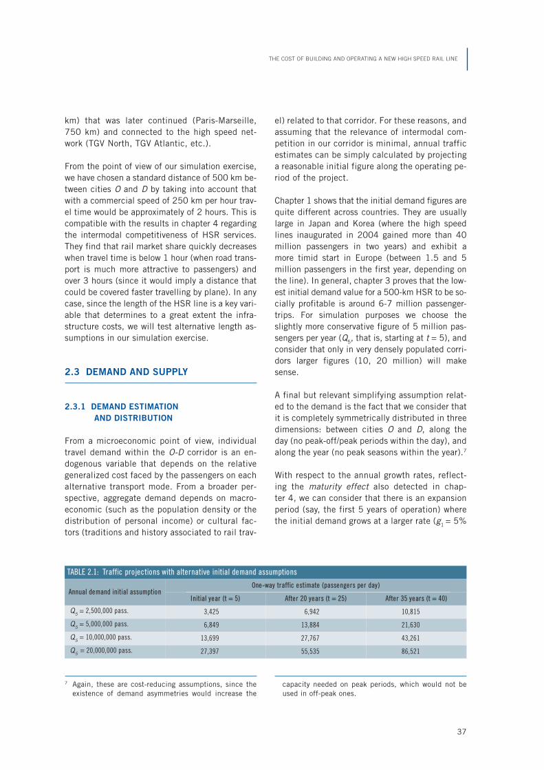
7 Again, these are cost-reducing assumptions, since theexistence of demand asymmetries would increase the

capacity needed on peak periods, which would not beused in off-peak ones.

km) that was later continued (Paris-Marseille,750 km) and connected to the high speed net-work (TGV North, TGV Atlantic, etc.).

From the point of view of our simulation exercise,we have chosen a standard distance of 500 km be-tween cities O and D by taking into account thatwith a commercial speed of 250 km per hour trav-el time would be approximately of 2 hours. This iscompatible with the results in chapter 4 regardingthe intermodal competitiveness of HSR services.They find that rail market share quickly decreaseswhen travel time is below 1 hour (when road trans-port is much more attractive to passengers) andover 3 hours (since it would imply a distance thatcould be covered faster travelling by plane). In anycase, since the length of the HSR line is a key vari-able that determines to a great extent the infra-structure costs, we will test alternative length as-sumptions in our simulation exercise.

2.3 DEMAND AND SUPPLY

2.3.1 DEMAND ESTIMATION

AND DISTRIBUTION

From a microeconomic point of view, individualtravel demand within the O-D corridor is an en-dogenous variable that depends on the relativegeneralized cost faced by the passengers on eachalternative transport mode. From a broader per-spective, aggregate demand depends on macro-economic (such as the population density or thedistribution of personal income) or cultural fac-tors (traditions and history associated to rail trav-

el) related to that corridor. For these reasons, andassuming that the relevance of intermodal com-petition in our corridor is minimal, annual trafficestimates can be simply calculated by projectinga reasonable initial figure along the operating pe-riod of the project.

Chapter 1 shows that the initial demand figures arequite different across countries. They are usuallylarge in Japan and Korea (where the high speedlines inaugurated in 2004 gained more than 40million passengers in two years) and exhibit amore timid start in Europe (between 1.5 and 5million passengers in the first year, depending onthe line). In general, chapter 3 proves that the low-est initial demand value for a 500-km HSR to be so-cially profitable is around 6-7 million passenger-trips. For simulation purposes we choose theslightly more conservative figure of 5 million pas-sengers per year (Q5, that is, starting at t = 5), andconsider that only in very densely populated corri-dors larger figures (10, 20 million) will makesense.

A final but relevant simplifying assumption relat-ed to the demand is the fact that we consider thatit is completely symmetrically distributed in threedimensions: between cities O and D, along theday (no peak-off/peak periods within the day), andalong the year (no peak seasons within the year).7

With respect to the annual growth rates, reflect-ing the maturity effect also detected in chap-ter 4, we can consider that there is an expansionperiod (say, the first 5 years of operation) wherethe initial demand grows at a larger rate (g1 = 5%


37

TABLE 2.1: Traffic projections with alternative initial demand assumptions

Annual demand initial assumptionOne-way traffic estimate (passengers per day)

Initial year (t = 5) After 20 years (t = 25) After 35 years (t = 40)

Q5 = 2,500,000 pass. 3,425 6,942 10,815

Q5 = 5,000,000 pass. 6,849 13,884 21,630

Q5 = 10,000,000 pass. 13,699 27,767 43,261

Q5 = 20,000,000 pass. 27,397 55,535 86,521

8 Daily traffic estimates are simply calculated by dividingannual demand between 365 days and between 2, since

the O-D traffic is symmetric.

from t = 6 to 11), while growing at a lower rate(g2 = 3%) afterwards.

With all these values, and departing from four al-ternative initial annual demand estimates (2.5,5, 10 and 20 million, respectively), table 2.1shows the resulting one-way traffic projections(in terms of passengers per day) at three differ-ent points: the start of the operating period, 20years later, and at the end of the project life-time.8 The variability is large; for example, if theinitial demand is 2.5 million passengers per year,at t = 40 it would imply a daily (one-way) trafficof 10,815 passengers; for 20 million, the corre-sponding value would be eight times larger(86,521).

These differences would be even worse if, alter-natively, the projections were made ignoring thematurity effect, that is, under the assumptionthat the demand grows at the same rate from t = 5to t = 40 (that is, g1 = g2 = 5%). Graph 2.2 showsthe corresponding (faster-growing) projections,where the final daily demands at t = 40 would

range from 18,890 (starting with 2.5 millionpassengers per year) to 151,124 (starting with20 million). Since these figures seem less realis-tic, our simulation exercise will be based on theprojections depicted in table 2.1.

2.3.2. SUPPLY PARAMETERS: TRAIN

CAPACITY AND FREQUENCY

If demand is measured as the daily number of(one-way) passengers, the corresponding defini-tion of supply is the number of seats offeredeveryday from O to D (or vice versa). Then, traincapacity and frequency become the key factorsthat determine the supply of HSR services in ourO-D corridor.

• TRAIN CAPACITY

The capacity (number of seats) of a train de-signed for HSR services depends on both the tech-nical specifications envisaged by the manufac-turer and the specific internal configuration agreedwith the prospective buyer. Nowadays most train


38

Graph 2.2 One-way traffic projections (under faster growth assumption)

Note: Vertical axis measures the number of passengers per day. Demand grows at 5% (t = 6-40).

0

50,000

100,000

150,000

200,000

250,000

300,000

0 2 4 6 8 10 12 14 16 18 20 22 24 26 28 30 32 34 36 38 40

2,500,000 pass. 5,000,000 pass. 10,000,000 pass. 20,000,000 pass.

9 It is unclear the net effect on costs associated to droppingthis assumption. On one hand, with higher-capacity trains,the total number of trains needed is reduced; but, on theother hand, their operating and maintenance costs couldbe larger, particularly if they are more intensively used.

10 As a quick reference, table 2.2 provides a summary of theparameter values for the reference case.

11 This is a low value when compared to the real world. Itcorresponds to an initial demand of 5,000,000 passen-gers per year. In subsequent years, when the demandgrows, the frequency (Ft) would also increase, reachingmore reasonable values of one service every 15 or lessminutes.

models can be easily adapted to project-specificneeds (legal requirements, cultural differences,passenger density, intensity of use, etc.), andtheir costs vary accordingly. In general three sizegroups can be identified in the existing manufac-turers catalogues: low-capacity trains (between200-250 seats), medium-capacity trains (be-tween 300-400 seats) and high capacity trains(more than 500 seats). The first group includes,for example, the ALARIS and TALGO units inSpain; the second group includes most models ofthe French TGV (including the THALYS), theSpanish AVE and some German ICE trains, whilethe TGV duplex and most Japanese units are inthe last group. For our simulation exercise we as-sume an average value of q– = 330 seats.

As mentioned above, there is a relevant simplify-ing assumption made here: we shall consider thatall trains in the fleet are exactly equal, and thatthey all operate in single composition. We ac-knowledge it is one of our less realistic assump-tions since in the real world, when demand growsover time the operator may respond by incorpo-rating higher-capacity trains or by operating theexisting ones in double composition, thus dupli-cating its supply. Despite its weakness, the as-sumption is necessary to keep the supply calcu-lations simple.9

• FREQUENCY

There are several alternative methods to calcu-late the number of seats (and, given their capac-ity, the number of trains) that the operator shouldprovide to service the daily demand. Our calcula-tions of the number of daily services and theirfrequency (defined as the number of services perhour) will be based on an average load factor of75% (l), which gives us the basic relationship be-tween supply and demand that will be main-tained throughout the exercise.

In the real world, most existing HSR services arecharacterized by relatively high load factors (wellabove 70%), or at least larger than other equiva-lent rail services. This is explained by the factthat HSR lines are specifically designed for pas-senger traffic in dense traffic corridors, with min-imal intermediate stops, and a marketing focuscentered on the travel time and price. In our par-ticular example—a direct service between O-Dwith a very regular and symmetric demand—theload factor must be large by definition. Howevernote that a load factor close to 100%, for exam-ple, is impractical because it would imply that alltrains would be always fully booked, and sometravellers could not use them.

Apart from our assumption of l =75%, a few oth-er values are needed. In particular, we will usethe average commercial speed of s = 250 km perhour (which yields a travel time of 2 hours per di-rection), and the train average capacity ofq– = 330 seats (which implies that the effectiveoccupation is q–e = 0.75 · 330 = 248 seats). Inaddition we consider that there is a boarding andtrain preparation time before each service of 15minutes (0.25 hours) and that trains operate 18hours a day (from 06:00 to 24:00).10

Using these values and departing from our pro-jections of the (one-way) daily demand (denotedby qt), the total number of daily services per di-rection is obtained from the ratio qt/q

–e. The fre-

quency (F) is then given by:

(qt /q–

e)Ft = ———— ,18

in terms of number of services per hour. For ex-ample, for the reference case, if q5= 6,849 pas-sengers, F5= 1.54 services per hour, which inturn implies a service every 39 minutes.11


39

12 This factor is quite firm-specific, and it is associatedwith the risk of failing to provide services vs. the cost ofacquiring, operating and maintaining an over-sized fleet.

The range of values found in the real world varies from1.25 to 1.6, depending on the corridor.


40

Since the demand is symmetric, and total traveltime of a return trip (including boarding times) is4h 30’ (x = 4.5 hours), the (minimum) number oftrains (of capacity q–, at speed s, and with a loadfactor of 75%) needed daily in the O-D corridor

xwould be given by the ratio ——— , that is

1 / Ft

qtx ——— .

18q–e

In order to face unforeseeable contingencies (de-lays, external damages, breakdowns, etc.) thisminimum number is multiplied by an (exoge-nous) contingency factor, which we will set in1.5.12 Thus, the supply (in terms of the numberof trains) would be finally given by:

qtRSt = (1.5) · x ——— ,18q–e

where RSt stands for rolling stock needed at t.

Graph 2.3 illustrates the supply calculationsresults and their evolution under alternativetrain capacity assumptions. Note that, for ex-ample, for the reference case (with q– = 330seats) our HSR service would start its opera-tions with 11 trains, but in t = 40 the figurewould be 33 due to the increase in the project-ed demand. With q– = 400 and q– = 500 the cor-responding initial values would be 9 and 7,whereas the final ones would be 28 and 22, re-spectively. These figures fit reasonably wellwith international standards, which sets thenumber of trains used for lines in the range of300-500 km (although with intermediate stopsand shorter legs) between 30 and 80 (around10-15 trains per 100 km of HSR line).

In practice, actual rolling stock provision in HSRlines around the world is directly affected by sev-eral project-specific parameters such as the aver-age commercial speed or the specific technologyused in each case. Other elements, such as theseasonality of demand or the existence of peakperiods, were ruled out from this exercise.

Graph 2.3 Number of trains needed under alternative capacity assumptions

0

5

10

15

20

25

30

35

330 seats 400 seats 500 seats

0 2 4 6 8 10 12 14 16 18 20 22 24 26 28 30 32 34 36 38 40

With respect to the first one, total travel time isreduced when average commercial speed is in-creased and vice versa, thus affecting the supplycalculations. Graph 2.4 illustrates these effectsby recalculating the number of trains needed un-der different speed assumptions. Obviously, thefigures in the reference case (250 km/h) are thesame as those in graph 2.3 with q– = 330. How-ever, note that if speed is reduced to an averageof 200 km/h (not an unrealistic assumption,nowadays) the number of trains needed at t = 40would jump to 41; on the other hand, increasing

the speed to 300 km/h would imply that 28trains (only five less than in the reference case)would be needed.

Finally, graph 2.5 shows the strong dependenceof the supply calculations with respect to the de-mand projections. It shows the number of trainsneeded every year under alternative values forinitial annual demand (as in table 2.1). Note, forexample, that departing from 2.5 million passen-gers per year, we will only need 6 trains in thefirst year (and 17 at t = 40). But if the initial de-


41

Graph 2.4 Number of trains needed under alternative speed assumptions

0

5

10

15

20

25

30

35

40

45

200 km/h 250 km/h 300 km/h

0 2 4 6 8 10 12 14 16 18 20 22 24 26 28 30 32 34 36 38 40

Graph 2.5 Number of trains needed under alternative initial annual demand assumptions

0

20

40

60

80

100

120

140

0 2 4 6 8 10 12 14 16 18 20 22 24 26 28 30 32 34 36 38 40

2,500,000 pass. 5,000,000 pass. 10,000,000 pass. 20,000,000 pass.

mand were 20 million, then the figures would be42 and 142. Therefore a wrong demand projec-tion could be more relevant for supply calcula-tions than changes in train capacity or in averagespeed.

2.4. METHODOLOGY OF COST

CALCULATIONS

2.4.1. OBJECTIVES

The main objective of this chapter is to providean estimate of the total cost of building, operat-ing and maintaining a HSR with technical char-acteristics and the supply and demand condi-tions described in the previous section. In orderto provide a quick reference to our referencecase, table 2.2 summarizes the main parametervalues considered in our analysis.

Although all these values can be individually mod-ified upwards or downwards—ceteris paribus—toillustrate their particular effect on our costs re-sults, we will restrict our comparative statics ex-ercises only to changes in the initial demand, thetrain capacity, the commercial speed, and theline length since these four factors summarizethe most salient economic characteristics of anyHSR line.

As described in section 2.1, cost calculationswill be categorized into two main groups: infra-structure costs and rolling stock costs, respec-tively denoted as IC and RSC. Thus, formally, thetotal cost (TC) of our HSR project (evaluated att = 0) is just given by the net present value:

T ICt + RSCtTC = R —————— . (2.1)

t=1 (1 + i)t

We now describe the components of each ofthese costs, and how each of them was calculat-ed in our particular example.

2.4.2. INFRASTRUCTURE COSTS

Infrastructure costs (IC) can be grouped into con-struction costs (ICC) and maintenance costs(ICM). Both of them are relatively independent onthe volume of the traffic and instead can be cal-culated as dependent on the line length (L), justby multiplying the number of kilometers by an av-erage unit cost (denoted as c and m, respective-ly). Construction costs spread out over the con-struction period whereas the maintenance takesplace during the operating period (see graph2.1). Formally, the infrastructure costs can bedenoted as

To (c · L)(1 + t)ICt = ICt

C + ICtM = R ——————— +

t=1 (1 + i)t

(2.2)T m · L

+ R ———— ,t=To+1 (1 + i)t

where we have additionally assumed that con-struction costs also include a surcharge (t =10%) to take into account planning costs.

The actual values of the average costs per km (c,m) were estimated from the values found inchapter 1 database of actual HSR projects. Inparticular, to err on the side of precaution, we did


42

TABLE 2.2: The reference case: main parameter values

Line length (L) = 500 km Train capacity (q–) =330 seats

Project timeline: t = 0 to t = 40 (T) Load factor (l) = 75%

Construction period (Tc) = 5 years Operating hours (daily) = 18 hours

Operation period (T – Tc) = 35 years Average commercial speed (s) = 250 km/h

Initial annual demand (Q5) = 5 mill. passengers Boarding time (between services) =15 minutes

Growth rate 1 (g1) = 5% (from t = 6 to 11) Train contingency factor = 50%

Growth rate 2 (g2) = 3% (from t = 12 to 40)

13 Note that it is equivalent to implicitly assume a probability distribution where the three cases are equally likely.

not considered just one value, but three: the low-est unit cost in the database (named, the bestscenario), the highest unit cost in the database(the worst scenario) and the average value in thedatabase (the medium scenario).13

Table 2.3 summarizes the results from thesecalculations for the reference case (where theline length is 500 km). The lowest construction(maintenance) cost per km is 9 million euros(12,919 euros, respectively), whereas the high-est is 39 million and 71,650, respectively.Note in table 2.4 that total infrastructure costsare fixed costs that evolve linearly with thelength of the corridor: for the largest case (650km) construction costs might reach a peak of€5,517 million per year in the worst scenario.

A final element to take into account in the previ-ous calculations is the residual value of the infra-structure at t = 40. This amount—once discount-

ed to t = 0—reduces the total cost of the infra-structure. In general, since there are different as-sets (tracks, buildings, etc.), with different use-ful lives and depreciation rates, it is quitedifficult to provide an accurate value of thisresidual value. To simplify calculations, we willjust assume that it will be equal to 30% of thetotal construction cost for each particular sce-nario. Thus for the reference case in the best sce-nario with a total building costs of €990 x 5years = €4,950 million, the residual value at t =40 is €1,485 million. The corresponding resid-ual values for the medium and worst scenarioswill be €2,700 and €5,850 million, respectively.

2.4.3. ROLLING STOCK COSTS

Rolling stock costs (RSC) can be grouped intothree categories: acquisition (RSCA), operation(RSCO) and maintenance (RSCM) of the trainsneeded to run the services. With respect to the


43

TABLE 2.3: Infrastructure costs per year (reference case)

Construction Maintenance

Period t = 1 to t = 5 t = 6 to t = 40

Line length (km) 500 500

Unit value (€ per km)

Best scenario 9,000,000 12,919

Medium scenario 18,000,000 35,624

Worst scenario 39,000,000 71,650

Planning cost (%) 10% —

Total value (€ per year)

Best scenario 990,000,000 6,459,500

Medium scenario 1,980,000,000 17,812,000

Worst scenario 4,290,000,000 35,825,000

TABLE 2.4: Annual infrastructure costs under different line lengths(euros)

L= 250 km L= 500 km L= 650 km

Building Maintenance Building Maintenance Building Maintenance

Best scenario 495,000,000 3,229,750 990,000,000 6,459,500 1,287,000,000 8,397,350

Medium scenario 990,000,000 8,906,000 1,980,000,000 17,812,000 2,574,000,000 23,155,660

Worst scenario 2,145,000,000 17,912,500 4,290,000,000 35,825,000 5,577,000,000 46,572,500

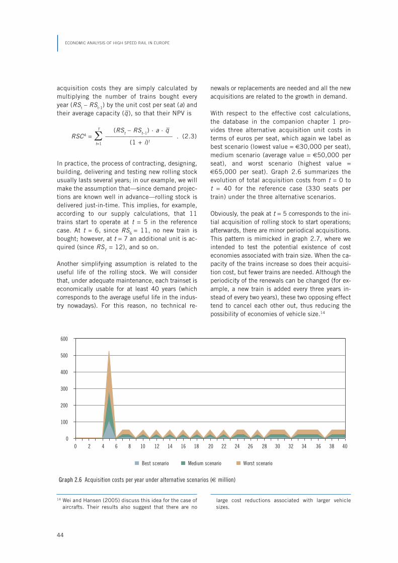
acquisition costs they are simply calculated bymultiplying the number of trains bought everyyear (RSt – RSt-1) by the unit cost per seat (a) andtheir average capacity (q–), so that their NPV is

T (RSt – RSt–1) · a · q–RSCA = R ——————————— . (2.3)

t=1 (1 + i)t

In practice, the process of contracting, designing,building, delivering and testing new rolling stockusually lasts several years; in our example, we willmake the assumption that—since demand projec-tions are known well in advance—rolling stock isdelivered just-in-time. This implies, for example,according to our supply calculations, that 11trains start to operate at t = 5 in the referencecase. At t = 6, since RS6 = 11, no new train isbought; however, at t = 7 an additional unit is ac-quired (since RS7 = 12), and so on.

Another simplifying assumption is related to theuseful life of the rolling stock. We will considerthat, under adequate maintenance, each trainset iseconomically usable for at least 40 years (whichcorresponds to the average useful life in the indus-try nowadays). For this reason, no technical re-

newals or replacements are needed and all the newacquisitions are related to the growth in demand.

With respect to the effective cost calculations,the database in the companion chapter 1 pro-vides three alternative acquisition unit costs interms of euros per seat, which again we label asbest scenario (lowest value = €30,000 per seat),medium scenario (average value = €50,000 perseat), and worst scenario (highest value =€65,000 per seat). Graph 2.6 summarizes theevolution of total acquisition costs from t = 0 tot = 40 for the reference case (330 seats pertrain) under the three alternative scenarios.

Obviously, the peak at t = 5 corresponds to the ini-tial acquisition of rolling stock to start operations;afterwards, there are minor periodical acquisitions.This pattern is mimicked in graph 2.7, where weintended to test the potential existence of costeconomies associated with train size. When the ca-pacity of the trains increase so does their acquisi-tion cost, but fewer trains are needed. Although theperiodicity of the renewals can be changed (for ex-ample, a new train is added every three years in-stead of every two years), these two opposing effecttend to cancel each other out, thus reducing thepossibility of economies of vehicle size.14


44

14 Wei and Hansen (2005) discuss this idea for the case ofaircrafts. Their results also suggest that there are no

large cost reductions associated with larger vehiclesizes.

Graph 2.6 Acquisition costs per year under alternative scenarios (€ million)

0

100

200

300

400

500

600

Best scenario Medium scenario Worst scenario

0 2 4 6 8 10 12 14 16 18 20 22 24 26 28 30 32 34 36 38 40

15 Note, for example, that a rolling stock unit bought at t = 40 has a residual value of 40/40 (that is, 100%).


45

Note that in the previous figures we have justconsidered the gross acquisition cost. If we as-sume that the average useful life of each rollingstock unit is 40 years, and that its value is re-duced 1/40 every year (linear depreciation), at t= 40 there will be some residual values that—once discounted to t = 0—should be reducedfrom the acquisition costs. These residual valuesdepend on the year each particular unit isbought. For example, in the reference case, theresidual value at t = 40 of the 11 trainset unitsacquired at t = 5 will be 5/40 of their acquisitioncost; the additional unit bought at t = 7 will beworth 7/40 of its initial cost, and so on.15 Byadding the residual values of all the units boughtfrom t = 5 to t = 40 we finally get the total resid-ual values (at t = 40) of the rolling stock undereach possible scenario: in the best one, it will be€149,242,500; in the medium scenario,€248,737,500, and in the worst scenario€323,358,750.

On the other hand, the operation and mainte-nance costs of the rolling stock are heavily de-pendent on the volume of traffic along the linewhich, indirectly, can be measured through thenumber of trains. In the case of the operationcosts (RSO), its main determinants are labor and

energy. The number of technical crew membersper train depends on its technical specificationsand is usually set in transport regulations. On thecontrary, there are no minimum standards oncabin attendants and auxiliary personnel, andtheir number depends on the level of service of-fered to passengers. Energy consumption is cal-culated in accordance with the technical specifi-cation of the rolling stock.For these reasons, in our simulation exercise, weused the expression:

T ro · RSt · q–RSCO = R —————— , (2.4)

t=5 (1 + i)t

where ro is the annual unit operation cost per seat(and the average train capacity). Once more, theactual value of ro is obtained from the database inchapter 1, which provides us with three alternativeestimates: best scenario (ro = €40,000 per seat),medium scenario (ro = €53,000 per seat), andworst scenario (ro = €65,000 per seat). The evolu-tion of total operation costs from t = 0 to t = 40for the reference case is given in graph 2.8.Interestingly, when the train size is increased (upto 400 and 500 seats), there are no clear costadvantages, as illustrated in graph 2.9 (drawn for

Graph 2.7 Acquisition costs per year under alternative train capacities (€ million)

0

100

200

300

400

500

600

0 2 4 6 8 10 12 14 16 18 20 22 24 26 28 30 32 34 36 38 40



46

the medium scenario only). In some years it ischeaper to operate larger sized trains, whereas inother years it is too expensive. It is important torecall here our simplifying assumption that alltrains are equal in size, which is somehow unre-alistic.

Finally, the maintenance costs of the rollingstock are not only related to traffic (measuredthrough the number of trains) but also to train in-

tensity usage. Thus a better estimate of the NPVof this cost would be given by

T rm · Dt · RStRSCM = R —————— , (2.5)t=5 (1 + i)t

where rm is the unit maintenance cost per train andkilometer, and Dt is the average distance travelled byeach train.16 According to chapter 1, rm can be esti-mated around €2/km for trains running around 0.5

Graph 2.8 Operation costs per year under alternative scenarios (€ million)

0

100

200

300

400

500

600

700

800

Best scenario Medium scenario Worst scenario

0 2 4 6 8 10 12 14 16 18 20 22 24 26 28 30 32 34 36 38 40

16 This average distance was calculated dividing the totaldistance covered by all trains every year (number of

total annual services multiplied by line length) betweenthe number of trains.

Graph 2.9 Operation costs per year under alternative train capacities (€ million)

150

200

250

300

350

400

450

500

550

600


0 2 4 6 8 10 12 14 16 18 20 22 24 26 28 30 32 34 36 38 40

million kilometers per year. For chapter 1, our refer-ence case, this value yields a total maintenance costof 20,202,020 euros at t = 5 and 63,798,448 eu-ros at t = 40. Note that, as depicted in graph 2.10,larger-size trains are cheaper to maintain, since theaverage distance they travel is lower.

2.5 CONCLUSIONS

By collecting together all the formulae and calcu-lations in the previous sections, our estimate ofthe total cost (at t = 0) of building, operating andmaintaining a HSR line would be obtained fromthe expression (2.1):

T ICtC + ICt

M + RSCtA

TC = R ——————————— +t=1 (1 + i)t

(2.6)RSCt

O + RSCtM

+ ——————— ,(1 + i)t

that is,

To (c · L)(1 + t) T m · LTC = R ——————— + R ———— +

t=1 (1 + i)tt=Tc+1 (1 + i)t

T (RSt – RSt–1) · a · q– T ro ·RSt · q–+ R —————————— + R ————— +

t=1 (1 + i)tt=5 (1 + i)t

T rm · Dt · RSt+ R ——————— . (2.7)t=5 (1 + i)t

Although it just provides a lower bound to the ac-tual cost, this expression summarizes the criticalfactors that must be taken into account when an-alyzing the costs of HSR lines. These include theline length (L), the number of trains needed torespond to the demand (RS), train capacity (q–),average distance (D) and the corresponding unitcosts (c, m, a, ro, rm).

Table 2.5 summarizes the numerical estimates ofthis total cost considering a discount rate (i) of5% under alternative assumptions on initial de-mand, train capacity, commercial speed and linelength. We also considered three scenarios re-garding the unit costs obtained from the data-base in chapter 1: the all-the-best scenario al-ways uses the lowest value of the unit costs ineach case; the all-the-medium scenario alwaysuses the average value of the unit costs in eachcase; and the all-the-worst scenario always usesthe highest value of the unit costs in each case.The implicit assumption behind these com-pound-scenarios is that there exists a perfectpositive correlation between all the unit costs: ifa country has a large construction cost, then itsoperating cost will be also large, and vice versa.In practice, this is not always the case since inseveral projects it is observed that the correlationcould be even negative.


47

Graph 2.10 Maintenance costs per year under alternative train capacities (€ million)

0

10

20

30

40

50

60

70

0 2 4 6 8 10 12 14 16 18 20 22 24 26 28 30 32 34 36 38 40


According to table 2.5, the total cost of a 40-yearHSR project lies between €7.7 and €23.7 billionin the reference case, depending on the scenario(best and worse, respectively). On average theNPV is 13.0 billion, which implies an average es-

timate of €25-30 million per kilometer. Table 2.5also shows that when the initial demand is halvedwith respect to the reference case (that is, only2.5 million passengers per year), the total cost isreduced (on average) just by a 20%, but if de-


48

TABLE 2.5 Total costs (at t=0) of a HSR line under alternative assumptions (euros)

All the best scenario All the medium scenario All the worst scenario

Initial demand assumptions

2,500,000 pass. 6,000,067,777 10,785,250,118 21,065,618,421

5,000,000 pass. 7,730,285,037 13,029,676,448 23,777,416,675

10,000,000 pass. 11,187,484,570 17,513,729,139 29,194,942,065

20,000,000 pass. 18,108,860,949 26,491,173,260 40,041,479,687

Train capacity assumptions

330 seats 7,730,285,037 13,029,676,448 23,777,416675

400 seats 7,648,681,646 12,945,753,435 23,691,415,005

500 seats 7,626,652,900 12,940,793,841 23,701,794,35

Commercial speed assumptions

200 km/h 8,390,219,242 13,913,020,245 24,863,968,621

250 km/h 7,730,285,037 13,029,676,448 23,777,416,675

300 km/h 7,277,305,302 12,423,499,186 23,031,845,523

Line length assumptions

250 km 4,080,508,403 6,803,021,727 12,243,154,507

500 km 7,730,285,037 13,029,676,448 23,777,416,675

650 km 9,909,604,536 16,751,534,490 30,680,581,170

Note: Results in bold correspond to the reference case.

Graph 2.11a NPV cost distribution depending on initial demand

46%

54%

33%

67%

24%

76%

63%

37%

49%

51%

38%

62%

77%

23%

65%

35%

55%

45%

87%

13%

79%

21%30%

70%

100%

75%

50%

25%

0%Bestcase

Avge.case

Worstcase

Bestcase

Avge.case

Worstcase

Bestcase

Avge.case

Worstcase

Bestcase

Avge.case

Worstcase

2,5 million pass. 5 million pass. 10 million pass. 20 million pass.

Fixed costs Variable costs

mand is duplicated (10 million passengers) totalcost can increase up to 31%. Similarly, it is inter-esting to note that neither the increase in train ca-pacity nor the commercial speed have a large im-pact reducing the total costs of the project. Their

effects on the supply tend to cancel out. On thecontrary, changes in the length of the line are crit-ical: shorter (larger) lines are dramatically cheap-er (more expensive) to build and operate whencompared to the reference case.


49

Graph 2.11b NPV cost distribution depending on commercial speed

100%

75%

50%

25%

0%Bestcase

Avge.case

Worstcase

Bestcase

Avge.case

Worstcase

Bestcase

Avge.case

Worstcase

200 km/h 250 km/h 300 km/h

80%

20%

69%

31%

58%

42%

77%

23%

65%

35%

55%

45%

74%

26%

61%

39%

51%

49%


Graph 2.11c NPV cost distribution depending on train capacity

100%

75%

50%

25%

0%Bestcase

Avge.case

Worstcase

Bestcase

Avge.case

Worstcase

Bestcase

Avge.case

Worstcase


77%

23%

66%

34%

56%

44%

77%

23%

66%

34%

56%

44%

77%

23%

65%

35%

55%

45%


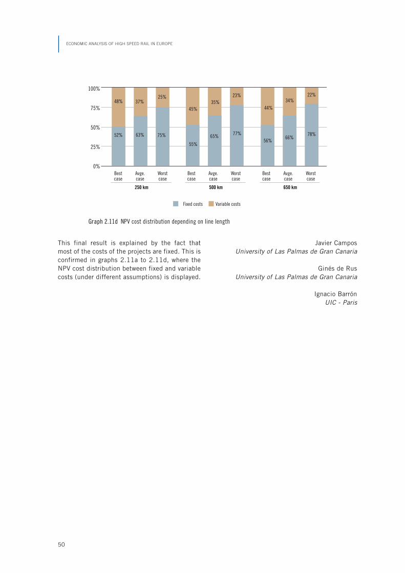
This final result is explained by the fact thatmost of the costs of the projects are fixed. This isconfirmed in graphs 2.11a to 2.11d, where theNPV cost distribution between fixed and variablecosts (under different assumptions) is displayed.



Ignacio BarrónUIC - Paris


50

Graph 2.11d NPV cost distribution depending on line length

100%

75%

50%

25%

0%Bestcase

Avge.case

Worstcase

Bestcase

Avge.case

Worstcase

Bestcase

Avge.case

Worstcase

250 km 500 km 650 km

78%

22%

66%

34%

56%

44%

77%

23%

65%

35%

55%

45%

75%

25%

63%

37%

52%

48%


3.1 INTRODUCTION

By High Speed Rail (HSR) we normally mean railtechnologies capable of speeds of the order of300km/h on new dedicated track. Such systemsoffer journey times that are more competitivewith other modes (and particularly air) than tra-ditional train services, and very high capacity.But their capital cost is also high. The proposalsof the European Commission for the Trans Euro-pean Transport Network (TEN-T) envisage expen-diture of 600 billion euros, of which 250 billioneuros is for priority projects, and a large part ofthis expenditure is for high speed rail. Thus it isextremely important to have a robust appraisalmethodology for these huge investments. It isnot clear that this has been the case of the TransEuropean Networks. Individual projects are sug-gested by, and appraised by, member state gov-ernments, even though they are applying for theEuropean Commission for assistance with fund-ing. Research for the European Commission hasappraised the TEN-T network as a whole, but hasnot appraised the individual elements of the pro-gram to ensure that they are all worthwhile (TML2005).

The aim of this chapter is to consider themethodology for the appraisal of high speed railproposals, and to produce some indication of thecircumstances in which such proposals might beworthwhile. In the next section, we present anoverview of the principal costs and benefitswhich need to be taken into account in a HSR ap-praisal. Then we illustrate the process for twoparticular contrasting examples: the study ofHSR proposals in Great Britain, and an ex postevaluation of the Madrid-Seville line in Spain. In

section 3.4, we formulate a model to incorporatethe principal parameters influencing the out-come of an appraisal and in section 3.5, we usethis model to draw conclusions on the circum-stances in which high speed rail may be justified.

3.2 OVERVIEW OF COSTS AND BENEFITS

3.2.1 OPTIONS TO CONSIDER

Appraisal requires comparison of a base casewith a series of do-something alternatives. It isnecessary to be clear what the base case is, andto ensure that a realistic range of options is ex-amined. A base case that literally assumes a do-nothing situation may be very unfavorable, par-ticularly in the face of growing traffic; on theother hand the base case should not be paddedout with unnecessary investments. In general thebase case should be a do-minimum option, andother likely investments should be examined asalternative do-something options. These alterna-tives should be compared on an incremental ba-sis to see whether the additional cost of movingto a more expensive option is justified.

In the case of high speed rail, the base caseshould therefore include such investment as it isnecessary to keep the existing service running,and consideration should be given to how to dealwith any exogenous growth in traffic. This mightmean investing in additional rolling stock or re-vising fares structures and levels. More majorchanges should be considered as do-somethingalternatives. These might include upgrading ex-isting infrastructure, purchase of a fleet of new

51

3

In What Circumstances is Investment

in HSR Worthwhile?

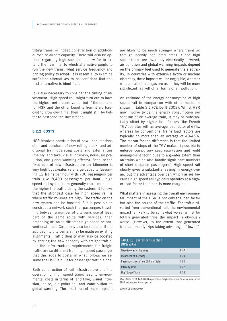
tilting trains, or indeed construction of addition-al road or airport capacity. There will also be op-tions regarding high speed rail—how far to ex-tend the new line, to which alternative points torun the new trains, what service frequency andpricing policy to adopt. It is essential to examinesufficient alternatives to be confident that thebest alternative is identified.

It is also necessary to consider the timing of in-vestment. High speed rail might turn out to havethe highest net present value, but if the demandfor HSR and the other benefits from it are fore-cast to grow over time, then it might still be bet-ter to postpone the investment.

3.2.2 COSTS

HSR involves construction of new lines, stationsetc., and purchase of new rolling stock, and ad-ditional train operating costs and externalities(mainly land take, visual intrusion, noise, air pol-lution, and global warming effects). Because thefixed cost of new infrastructure per kilometer isvery high but creates very large capacity (assum-ing 12 trains per hour with 700 passengers pertrain give 8,400 passengers per hour), highspeed rail systems are generally more economicthe higher the traffic using the system. It followsthat the strongest case for high speed rail iswhere traffic volumes are high. The traffic on thenew system can be boosted if it is possible toconstruct a network such that passengers travel-ling between a number of city pairs use at leastpart of the same route with services, thenbranching off on to different high speed or con-ventional lines. Costs may also be reduced if theapproach to city centers may be made on existingalignments. Traffic density may also be boostedby sharing the new capacity with freight traffic,but the infrastructure requirements for freighttraffic are so different from high speed passengerthat this adds to costs; in what follows we as-sume the HSR is built for passenger traffic alone.

Both construction of rail infrastructure and theoperation of high speed trains lead to environ-mental costs in terms of land take, visual intru-sion, noise, air pollution, and contribution toglobal warming. The first three of these impacts

are likely to be much stronger where trains gothrough heavily populated areas. Since highspeed trains are invariably electrically powered,air pollution and global warming impacts dependon the primary fuel used to generate the electric-ity; in countries with extensive hydro or nuclearelectricity, these impacts will be negligible, whereaswhere coal, oil and gas are used they will be moresignificant, as will other forms of air pollution.

An estimate of the energy consumption of highspeed rail in comparison with other modes isshown in table 3.1 (CE Delft 2003). Whilst HSRmay involve twice the energy consumption perseat km of an average train, it may be substan-tially offset by higher load factors (the FrenchTGV operates with an average load factor of 67%,whereas for conventional trains load factors aretypically no more than an average of 40-45%.The reason for the difference is that the limitednumber of stops of the TGV makes it possible toenforce compulsory seat reservation and yieldmanagement techniques to a greater extent thanon trains which also handle significant numbersof short distance passengers.) High speed railclearly gives a substantial saving in energy overair, but the advantage over car, which arises be-cause high speed rail typically operates at a high-er load factor than car, is more marginal.

What matters in assessing the overall environmen-tal impact of the HSR is not only the load factorbut also the source of the traffic. For traffic di-verted from conventional rail, the environmentalimpact is likely to be somewhat worse, whilst fortotally generated trips the impact is obviouslyworse. (However, to the extent that generatedtrips are mainly trips taking advantage of low off-


52

TABLE 3.1: Energy consumption(MJ/Seat Km)

Gasoline car on highway 0.47

Diesel car on highway 0.34

Passenger aircraft on 500 km flight 1.80

Intercity Train 0.22

High Speed Train 0.53

Note: Based on CE Delft (2003) Appendix A. Graphs for car are based on new cars in2000 and assume 5 seats per car.

Source: CE Delft (2003).

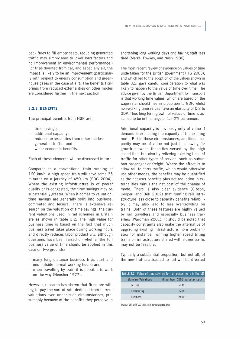
peak fares to fill empty seats, reducing generatedtraffic may simply lead to lower load factors andno improvement in environmental performance.)For trips diverted from car, and especially air, theimpact is likely to be an improvement (particular-ly with respect to energy consumption and green-house gases in the case of air). The benefits HSRbrings from reduced externalities on other modesare considered further in the next section.

3.2.3 BENEFITS

The principal benefits from HSR are:

— time savings;— additional capacity;— reduced externalities from other modes;— generated traffic; and— wider economic benefits.

Each of these elements will be discussed in turn.

Compared to a conventional train running at160 km/h, a high speed train will save some 35minutes on a journey of 450 km (SDG 2004).Where the existing infrastructure is of poorerquality or is congested, the time savings may besubstantially greater. When it comes to valuation,time savings are generally split into business,commuter and leisure. There is extensive re-search on the valuation of time savings; the cur-rent valuations used in rail schemes in Britainare as shown in table 3.2. The high value forbusiness time is based on the fact that muchbusiness travel takes place during working hoursand directly reduces labor productivity, althoughquestions have been raised on whether the fullbusiness value of time should be applied in thiscase on two grounds:

— many long distance business trips start andend outside normal working hours; and

— when travelling by train it is possible to workon the way (Hensher 1977).

However, research has shown that firms are will-ing to pay the sort of rate deduced from currentvaluations even under such circumstances, pre-sumably because of the benefits they perceive in

shortening long working days and having staff lesstired (Marks, Fowkes, and Nash 1986).

The most recent review of evidence on values of timeundertaken for the British government (ITS 2003),and which led to the adoption of the values shown intable 3.2, gave careful consideration to what waslikely to happen to the value of time over time. Theadvice given by the British Department for Transportis that working time values, which are based on thewage rate, should rise in proportion to GDP, whilstnon-working time values have an elasticity of 0.8 toGDP. Thus long term growth of values of time is as-sumed to be in the range of 1.5-2% per annum.

Additional capacity is obviously only of value ifdemand is exceeding the capacity of the existingroute. But in those circumstances, additional ca-pacity may be of value not just in allowing forgrowth between the cities served by the highspeed line, but also by relieving existing lines oftraffic for other types of service, such as subur-ban passenger or freight. Where the effect is toallow rail to carry traffic, which would otherwiseuse other modes, the benefits may be quantifiedas the net user benefits plus net reduction in ex-ternalities minus the net cost of the change ofmode. There is also clear evidence (Gibson,Cooper, and Bell 2002) that running rail infra-structure less close to capacity benefits reliabili-ty; it may also lead to less overcrowding ontrains. Both of these features are highly valuedby rail travellers and especially business trav-ellers (Wardman 2001). It should be noted thatcapacity constraints also make the alternative ofupgrading existing infrastructure more problem-atic; for instance, running higher speed tiltingtrains on infrastructure shared with slower trafficmay not be feasible.

Typically a substantial proportion, but not all, ofthe new traffic attracted to rail will be diverted

IN WHAT CIRCUMSTANCES IS INVESTMENT IN HSR WORTHWHILE?

53

Source: DfT: WEBTAG Unit 3.5.6 (www.webtag.org)

TABLE 3.2: Value of time savings for rail passengers in the UK

Standard Valuations (£ per hour, 2002 market prices)

Leisure 4.46

Commuting 5.04

Business 39.96

from other modes—mainly car and air (Britishstudies, such as Atkins 2003, suggest that thismay be of the order of 50%, with the remainderbeing totally new trips). To the extent that infra-structure charging on these modes does not coverthe marginal social cost of the traffic concerned,there will be benefits from such diversion. Esti-mation of these benefits requires valuation ofmarginal costs of congestion, noise, air pollution,global warming, and external costs of accidentsand their comparison with taxes and charges.

INFRAS/IWW (2000) provides estimates of mar-ginal external cost per passenger km for two Eu-ropean corridors, including accidents and envi-ronmental cost but excluding congestion. Theseare reproduced in table 3.3, and show the highspeed rail between Paris and Brussels to haveless than a quarter of the external cost of car orair. Higher load factors mean that HSR´s per-formance on such corridor is no worse than thatof conventional rail on the (much longer) Paris-Viena corridor. On longer distances, the advan-tage over air diminishes since most of the envi-ronmental costs of air transport are incurredduring take-offs and landings.

In the case of air, the absence of fuel tax meansthat there is normally no charge for environmen-tal externalities, although this is crudely allowedfor in some countries (including Britain) by a de-parture tax. (Value added tax [VAT] at the stan-dard rate should not be seen as an externalitycharge since it does not influence relative prices,except when charged on some modes and notothers; in some cases in Europe VAT is chargedon domestic rail and air fares, in some on rail butnot air and in others on neither).

The other key issue for air is charging for slots atcongested airports. The allocation of slots bygrandfather rights and charging structures, basedon average costs of running the airport (or lesswhere there are subsidies), mean that chargesmay not reflect congestion costs imposed on oth-er planes, the opportunity cost of slots or thecosts of expanding capacity. A further benefit ofhigh speed rail may therefore be the release ofcapacity at airports for use by other, typicallylonger distance flights. Regarding accidents,there has never yet been a fatality on a purpose-built HSR, and the record of conventional rail ismuch better than car, though not bus or particu-larly air (Evans 2003).

Generated traffic leads directly to benefits tousers, which are generally valued at half the ben-efit to existing users according to the rule of ahalf. But there has been much debate as towhether these generated trips reflect wider eco-nomic benefits that are not captured in a tradi-tional cost benefit analysis. Leisure trips maybenefit the destination by bringing in touristspending; commuter and business trips reflect ex-pansion or relocation of jobs or homes or addition-al economic activity.

The debate on these issues centers on whetherthese changes really are additional economic ac-tivity or whether such activity is simple relocat-ed. In a perfectly competitive economy with noinvoluntary unemployment, theory tells us thatthere would be no net benefit. In practice, thereare reasons why there may be additional benefits.Firstly, if the investment relocates jobs to de-pressed areas, it may reduce involuntary unem-ployment. The experience of Lille, which hasbeen regenerated by its location at the crossroadsof high speed lines between Paris, Brussels andLondon is often cited as an example. High speedrail tends to favor central locations, so if the aimis to regenerate major cities then it may be ben-eficial. However, if the depressed areas are at theperiphery, this is the opposite of what is desired.High speed rail may also allow for expanded mar-ket areas and the exploitation of economies ofscale, reducing the impact of imperfect competi-tion, and encouraging the location of jobs in ma-jor urban centers where there are external bene-fits of agglomeration (Graham 2005). Any such


54

TABLE 3.3: External costs(euros/1,000 pass-km)

Paris-Vienna Paris-Brussels

Car 40.2 43.6

Rail 11.7 10.4

Air 28.7 47.5

Note: The measured externalities include accidents, noise, air pollution, climatechange, urban effects, and upstream/downstream effects, but not congestion orscarce capacity.

Source: INFRAS/IWW (2000).

impacts are most likely to be found in the case ofservice industries (Bonnafous 1987).

Chapter 5 concludes that HSR may have addi-tional benefits for the above-mentioned reasons,but that the effects are very variable and difficultto predict. They are likely to be much less impor-tant than the direct transport benefits of HSR;typically they will also apply to alternative trans-port infrastructure investments, so that whilstthey improve the case for transport investment asa whole, they do not necessarily benefit HSRagainst other modes.

Another key factor influencing the outcome of anappraisal is the choice of discount rate. Low dis-count rates favor capital intensive investments suchas HSR. Practice varies substantially within the Eu-ropean Union. In Britain the current practice is todiscount at a pure time preference rate of discountof 3.5%, reducing to 3% after 30 years, but to al-low for capital shortages by requiring a benefit/costratio of at least 1.5 and preferring projects where itis at least 2. DG Regio recommends a 5% social dis-count rate. Given that HSR is very capital intensive

and has a long life with growing benefits over time,a low discount rate will favor investment in HSR.

3.3 EMPIRICAL EXAMPLES

In this section we will examine two empiricalcase studies, in radically different circumstancesand with widely differing results. Firstly we lookat a study of a new North-South high speed railline in Britain, undertaken for the Strategic RailAuthority by a consortium led by the consultantsW.S. Atkins (SRA). Then we look at a study of theactual Madrid-Seville line.

3.3.1 BRITISH HSR PROPOSALS

The Atkins study took place in a context of rapidgrowth in rail passenger and freight traffic in re-cent years (graph 3.1), leading to severe over-crowding on both long distance passenger servic-es and London commuter services, and a lack ofcapacity for further growth in freight. Thus a ma-jor objective of the scheme was to relieve exist-


55

Graph 3.1 Rail Passenger and Freight Volumes (1979 to 2004/05)

Note: The Hatfield accident in October 2000 led to severe speed restrictions being imposed which temporarily halted traffic growth.

Source: Transport Trends, 2002 Edition. Departmant for Transport and National Rail Trends, SRA.

0.0

5.0

10.0

15.0

20.0

25.0

30.0

35.0

40.0

45.0

1979

1980

1981

1982

1983

1984

/85

1985

/86

1986

/87

1987

/88

1988

/89

1989

/90

1990

/91

1991

/92

1992

/93

1993

/94

1994

/95

1995

/96

1996

/97

1997

/98

1998

/99

1999

/00

2000

/01

2001

/02

2002

/03

2003

/04

2004

/05

Bill

ion

Pass

enge

r-Km

and

Bill

ion

Frei

ght

Tonn

e-Km

Passenger-Kilometers

Freight (Net) Tonne-Kilometers

Post-privatization period

Post-

Hatfield

period

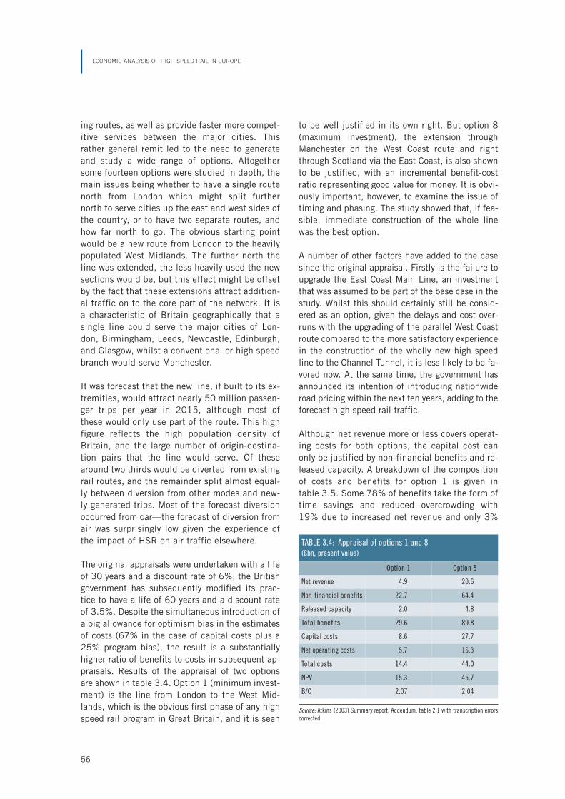
ing routes, as well as provide faster more compet-itive services between the major cities. Thisrather general remit led to the need to generateand study a wide range of options. Altogethersome fourteen options were studied in depth, themain issues being whether to have a single routenorth from London which might split furthernorth to serve cities up the east and west sides ofthe country, or to have two separate routes, andhow far north to go. The obvious starting pointwould be a new route from London to the heavilypopulated West Midlands. The further north theline was extended, the less heavily used the newsections would be, but this effect might be offsetby the fact that these extensions attract addition-al traffic on to the core part of the network. It isa characteristic of Britain geographically that asingle line could serve the major cities of Lon-don, Birmingham, Leeds, Newcastle, Edinburgh,and Glasgow, whilst a conventional or high speedbranch would serve Manchester.

It was forecast that the new line, if built to its ex-tremities, would attract nearly 50 million passen-ger trips per year in 2015, although most ofthese would only use part of the route. This highfigure reflects the high population density ofBritain, and the large number of origin-destina-tion pairs that the line would serve. Of thesearound two thirds would be diverted from existingrail routes, and the remainder split almost equal-ly between diversion from other modes and new-ly generated trips. Most of the forecast diversionoccurred from car—the forecast of diversion fromair was surprisingly low given the experience ofthe impact of HSR on air traffic elsewhere.

The original appraisals were undertaken with a lifeof 30 years and a discount rate of 6%; the Britishgovernment has subsequently modified its prac-tice to have a life of 60 years and a discount rateof 3.5%. Despite the simultaneous introduction ofa big allowance for optimism bias in the estimatesof costs (67% in the case of capital costs plus a25% program bias), the result is a substantiallyhigher ratio of benefits to costs in subsequent ap-praisals. Results of the appraisal of two optionsare shown in table 3.4. Option 1 (minimum invest-ment) is the line from London to the West Mid-lands, which is the obvious first phase of any highspeed rail program in Great Britain, and it is seen

to be well justified in its own right. But option 8(maximum investment), the extension throughManchester on the West Coast route and rightthrough Scotland via the East Coast, is also shownto be justified, with an incremental benefit-costratio representing good value for money. It is obvi-ously important, however, to examine the issue oftiming and phasing. The study showed that, if fea-sible, immediate construction of the whole linewas the best option.

A number of other factors have added to the casesince the original appraisal. Firstly is the failure toupgrade the East Coast Main Line, an investmentthat was assumed to be part of the base case in thestudy. Whilst this should certainly still be consid-ered as an option, given the delays and cost over-runs with the upgrading of the parallel West Coastroute compared to the more satisfactory experiencein the construction of the wholly new high speedline to the Channel Tunnel, it is less likely to be fa-vored now. At the same time, the government hasannounced its intention of introducing nationwideroad pricing within the next ten years, adding to theforecast high speed rail traffic.

Although net revenue more or less covers operat-ing costs for both options, the capital cost canonly be justified by non-financial benefits and re-leased capacity. A breakdown of the compositionof costs and benefits for option 1 is given intable 3.5. Some 78% of benefits take the form oftime savings and reduced overcrowding with19% due to increased net revenue and only 3%


56

TABLE 3.4: Appraisal of options 1 and 8(£bn, present value)

Option 1 Option 8

Net revenue 4.9 20.6

Non-financial benefits 22.7 64.4

Released capacity 2.0 4.8

Total benefits 29.6 89.8

Capital costs 8.6 27.7

Net operating costs 5.7 16.3

Total costs 14.4 44.0

NPV 15.3 45.7

B/C 2.07 2.04

Source: Atkins (2003) Summary report, Addendum, table 2.1 with transcription errorscorrected.

1 See De Rus and Inglada (1993, 1997).2 Price discounts of up to 30% (Madrid-Seville) and 50%

(Madrid-Ciudad Real) were introduced to compensate the

reduction in demand after EXPO closure (in October,1992). These discounts contributed to higher load fac-tors.

taking the form of reduced road congestion andaccidents. The value of the released capacity wasnot included in this analysis, but adds some 7%to the overall benefits.

On balance it was thought that the non-quanti-fied environmental benefits were slight. It is aninteresting question whether more of the userbenefits could be captured as revenue by moresophisticated yield management techniques thanthe simple fare structure model. Such yield man-agement methods are already in use on otherhigh speed services, including Eurostar servicesbetween London, Paris, and Brussels. They mightalso boost benefits by increasing diversion fromair; in the study this was found to be rather smallon the assumption that rail fares would on aver-age exceed those by air for traffic between Lon-don and Scotland.

In summary, then, this study of Britain found astrong case for high speed rail, based on the highpatronage that could be attracted by a single line

linking most of the major conurbations of Britain,in the context of growing demand leading to se-vere overcrowding and shortages of capacity onthe existing infrastructure. In the following sec-tion we look at a contrasting situation—that ofSpain.

3.3.2 THE SPANISH EXPERIENCE1

The construction of the first high speed line inSpain was carried out between 1987 and 1993.The Madrid-Seville line started its operations inApril 1992, with a demand highly influenced bythe Universal Exhibition held in Seville in 1992(EXPO) and with the pricing policy applied byRENFE. The Madrid-Seville corridor includes sev-eral routes2 (commuting, long-distance and serv-ices provided to other destinations using high-speed infrastructure but with Talgo technology).

High speed train is the transport option with thelowest generalized cost in this corridor, but notthe fastest mode. Air transport has the lowesttravel time in the Madrid-Seville corridor, afteraccounting for access and waiting times. The ad-vantage of the HSR with respect to air transportappears when tariffs of both modes are com-pared. These differences in the generalized costshave induced changes in the modal split to thebenefit of HSR. Diverted traffic comes mainlyfrom conventional train and air transport.

Regarding the impact of the Madrid-Seville HSRon other transport operators, the main effectswhich must be considered are those on air trans-port (Iberia and airports), on conventional rail-ways, and on road transport. For air transport be-tween Madrid and Seville, the introduction of theHSR induced a demand downshift of 50%, di-minishing the load factor and flight frequency.The Seville airport suffered a reduction of 25%in its use, as Madrid-Seville represented 50% ofairport traffic. Given the investments which werecarried out in the airport of Seville to accommo-date the peak of demand induced by the exhibi-tion EXPO-92, and more recent investment at


57

TABLE 3.5: Cost benefit analysis results, option 1(% of Total Benefits or Costs)

Benefits – Revenue

HSR Revenue 64%

Classic rail revenue –45%

Net rail revenue 19%

Benefits – Users

Journey time/reduced overcrowding 76%

Accidents 2%

Total User Benefits 78%

Benefits – Non-users

Journey time/veh operating costs 3%

Total Non-User Benefits 3%

Present Value Benefits 100%

Costs

Capital 69%

HSR operating 41%

Classic operating –9%

Present Value Costs 100%

Source: Atkins (2003) unpublished full report.

Barajas airport in Madrid, it is unlikely that thisdiversion will significantly reduce congestion al-though it will certainly reduce pollution from airtransport.

For conventional railway transport, RENFE wasalso affected by the introduction of the new prod-uct. The Madrid-Seville, Madrid-Malaga andMadrid-Cordoba links were amongst the maintwenty lines of the company. Conventional trainshave lost the major part of their traffic in this cor-ridor; therefore an efficient solution might be toconsider the closure of the conventional infra-structure. However, the impossibility of carryinggoods on the new infrastructure makes this sce-nario unfeasible.

HSR long distance services and bus transport arehardly substitutes at current prices. In commuterservices, and taking into account the low pricesintroduced by RENFE, bus operators are certain-ly affected by HSR.

Given the demand volumes in this corridor, themain benefits obtained from the investment inhigh speed rail are derived from time savings ob-tained when users shift from slower transportmodes, and gains from generated traffic. It hasalso been argued that one of the key benefits ofHSR was the increase of land value in CiudadReal. Nevertheless, this benefit is a consequenceof the improvement in accessibility to this city,which is already accounted for in the reduction oftravel time between Madrid and Ciudad Real. Toinclude this effect in the analysis would lead todouble counting.

To evaluate the economic effects of HSR, it is re-quired first to have an estimation of the demandfor the period which is going to be considered forthe analysis. To obtain this estimate, surveys car-ried out by RENFE in the Madrid-Seville corridorwere consulted, and real data of HSR for the pe-riod 1992–1994 and four months in 1995 wereused. Additional information was supplied byIberia, RENFE, and bus companies operating inthe corridor. The main components of the de-mand (generated and diverted traffic) were ob-tained for each market segment (commuters,long distance and Talgo) and each transportmode.

The evolution of demand for the 30-year projectlife (40 years in the sensitivity analysis) is esti-mated assuming that the Spanish GDP will growfrom 1997 onwards at a rate of 2.5%, the elas-ticity of demand with respect to GDP is assumedto be 1.25, and that HSR fares will not be re-duced below average variable costs.

Using this demand estimation, the social prof-itability of the HSR was estimated. Benefits ofthe HSR are obtained from 1992 onwards, afterthe starting of the service. Costs and benefitpresent values are discounted with a 6% socialdiscount rate.

The HSR costs have a fixed component (infra-structure), semi-fixed (trains) and variable (oper-ating costs). In this evaluation it is consideredthat prices (net of tax) of the infrastructure,trains and operating costs measure opportunitycosts except in the case of labor. HSR infrastruc-ture was built between 1987 and 1992, its costs(including taxes) was 500 billion pesetas at1996 currency value. HSR benefits are mainlyobtained from time savings and generated traffic.

Benefits and costs of the first HSR line in Spainare summarized in Table 3.6. The NPV is –258 bil-lion pesetas at 1987 prices, using a social dis-count rate of 6%. Table 3.5 shows the sensitivityof results to different assumptions: life of the proj-ect (40 years); shadow pricing of labor; increase of25% in generalized costs of car, train and bus;and GDP growing at a 3% rate. These changes donot affect the main findings of this evaluation.

A simple financial analysis of the project shows aNPV of –314 billion pesetas in 1987, which in-dicates that an economic evaluation of HSR, con-sidering all social costs and benefits, reveals an18% improvement on its performance. As table3.5 shows, the main source of benefits of theHSR is generated traffic (44% of the total bene-fits of the project).

Benefits of diverted traffic are not limited to timesavings (22.5% of total benefits). The reductionin operating cost in other transport modes is alsoimportant. The shift to HSR of journeys by carforms 8.9% of the total benefits; cost savingsfrom railway and air transport yield benefits of


58

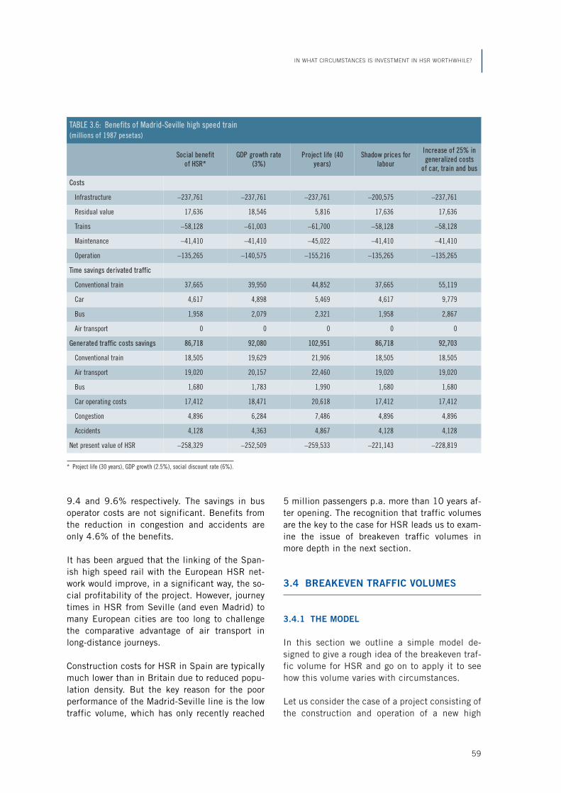
9.4 and 9.6% respectively. The savings in busoperator costs are not significant. Benefits fromthe reduction in congestion and accidents areonly 4.6% of the benefits.

It has been argued that the linking of the Span-ish high speed rail with the European HSR net-work would improve, in a significant way, the so-cial profitability of the project. However, journeytimes in HSR from Seville (and even Madrid) tomany European cities are too long to challengethe comparative advantage of air transport inlong-distance journeys.

Construction costs for HSR in Spain are typicallymuch lower than in Britain due to reduced popu-lation density. But the key reason for the poorperformance of the Madrid-Seville line is the lowtraffic volume, which has only recently reached

5 million passengers p.a. more than 10 years af-ter opening. The recognition that traffic volumesare the key to the case for HSR leads us to exam-ine the issue of breakeven traffic volumes inmore depth in the next section.

3.4 BREAKEVEN TRAFFIC VOLUMES

3.4.1 THE MODEL

In this section we outline a simple model de-signed to give a rough idea of the breakeven traf-fic volume for HSR and go on to apply it to seehow this volume varies with circumstances.

Let us consider the case of a project consisting ofthe construction and operation of a new high


59

TABLE 3.6: Benefits of Madrid-Seville high speed train(millions of 1987 pesetas)

Social benefitof HSR*

GDP growth rate(3%)

Project life (40years)

Shadow prices forlabour

Increase of 25% in generalized costs

of car, train and bus

Costs

Infrastructure –237,761 –237,761 –237,761 –200,575 –237,761

Residual value 17,636 18,546 5,816 17,636 17,636

Trains –58,128 –61,003 –61,700 –58,128 –58,128

Maintenance –41,410 –41,410 –45,022 –41,410 –41,410

Operation –135,265 –140,575 –155,216 –135,265 –135,265

Time savings derivated traffic

Conventional train 37,665 39,950 44,852 37,665 55,119

Car 4,617 4,898 5,469 4,617 9,779

Bus 1,958 2,079 2,321 1,958 2,867

Air transport 0 0 0 0 0

Generated traffic costs savings 86,718 92,080 102,951 86,718 92,703

Conventional train 18,505 19,629 21,906 18,505 18,505

Air transport 19,020 20,157 22,460 19,020 19,020

Bus 1,680 1,783 1,990 1,680 1,680

Car operating costs 17,412 18,471 20,618 17,412 17,412

Congestion 4,896 6,284 7,486 4,896 4,896

Accidents 4,128 4,363 4,867 4,128 4,128

Net present value of HSR –258,329 –252,509 –259,533 –221,143 –228,819

* Project life (30 years), GDP growth (2.5%), social discount rate (6%).

3 We drop this assumption later.4 The HSR can be vertically integrated or separated. All

high speed rail lines in the world currently operate asvertically integrated firms. Vertical unbundling is one ofthe key elements of EU railway policy, and proposals areunder consideration to allow open access for new entrantsinto the international rail passenger market.

5 We ignore here environmental impacts, such as land-

take, barrier effect, noise, and visual intrusion, whichshould also be accounted for on the cost side of HSR,as well as on the benefit side when HSR is a substituteof a highway or an airport.

6 We are not maximizing welfare but obtaining a changein welfare when the government decides to build a newhigh speed railway line.

speed railway line. This project has a life of Tyears. The construction firm builds the rail infra-structure and superstructure, and the operatorbuys the rolling stock during some initial period,which will be considered as the year of reference(t = 0) and thereafter when it requires replace-ment. From t = 0 to t = T, the railway operatorcharges a regulated fare and each year receives Qusers, assumed to be constant during the life ofthe project.3

Investment costs (construction and the presentvalue of rolling stock), expressed as opportunitycosts, are equal to I, evaluated in constant termsof year t = 0. During the life of the project, the op-erator4 incurs some annual costs of maintainingand operating the rail track, stations, signallingand other fixed plants, and the operating costs oflabor and energy consumed in train operation.Some maintenance costs (track, stations, rollingstock) are fixed (Ct(t)) and thus invariable to thelevel of traffic Q, and others are demand related,depending on the number of users (Cq(Q)). Allcosts are computed at opportunity costs.

Investment in HSR consist of building a new lineand operating high speed rolling stock which re-duces the time component of the generalized costfor all passengers switching from the convention-al mode to the new mode and, thus, affecting oth-er secondary markets, whose products or servicesare complements or substitutes of the HSR serv-ice, including those users who continue using theconventional mode,5 road users, for example, be-cause congestion is eased. This investment gen-erates some net benefits in the primary market,and some indirect benefits in secondary markets.

Total costs of the project are:

I + y0

T (Ct + Cq(Q))e–rt dt , (3.1)

where:

I: investment costs;

Ct: annual fixed maintenance and operating cost;

Cq(Q): annual maintenance and operating costvariable with Q;

T: project life;

r: social discount rate.

The introduction of a HSR line means a discretereduction of the generalized cost of travel. Giventhat HSR is an indivisible investment, thechange in social surplus is the following:6

ΔW = y0

T yg1

g0 Q(g)e–rtdgdt + y

0

T [p–(Q1 – Q0) –

– Ct – Cq(Q1) + CC(Q0)]e–rtdt – I + (3.2)

N

+ R y0

T Si(qi1 – qi0)e–rtdt ,

i=1

where:

go: generalized cost without the HSR project;

g1: generalized cost with the HSR project;

p–: regulated fare;

Q0: demand without the HSR project;

Q1: demand with the HSR project (includes di-verted and generated traffic);



CC(Q): annual avoidable cost of the conventionalmode;


60

7 This is especially relevant for freight transport. TheBritish Department of Transport suggests an additional6% of net benefits in UK due to the expansion of de-mand in monopolistic sectors which benefit from trans-

port reduction projects (see Department of Environ-ment, Transport and the Regions 1999).

8 These constitute net benefits which are yet to be meas-ured in the primary market.

I: infrastructure construction costs;

N: other markets in the economy;

Si: excess of benefits over costs of a unit changein qi;

qi0: level of activity in market i without the project;

qi1: level of activity in market i with the project;

T: project life;

r: social discount rate.

Expression (3.2) shows how the introduction ofthe HSR line affects transport users and produc-ers in the primary markets, with annual benefitsmeasured by the definite integral between theinitial generalized cost (g0) and the new one (g1),once the HSR line is introduced. Producer sur-plus can be measured through annual revenueand avoidable cost changes. Then, HSR invest-ment cost (I) has to be deducted from the dis-counted flows of these benefits.

The demand function for transport Q(g) is a de-rived demand, and one should be careful whenadding the indirect effects of the reduction intravel time in competitive markets, where firmsuse transport as an input to avoid double count-ing (see Jara-Díaz 1986); so, we will limit our at-tention to secondary markets, where products andservices are related to the primary market throughcomplementarity or substitutability links, or inthe case of monopolistic firms using the HSRservice as an input.

The third line of expression (3.2) accounts for indi-rect or secondary benefits. There are N secondarymarkets in the economy, which may have their lev-el of demand affected by the new project. Thechange in the level of activity in these secondarymarkets would affect the NPV of the project as longas there is an excess of benefits over costs of a unit

change of q, represented by Si which could be pos-itive or negative (Harberger 1972; Mohring 1976).

Therefore the justification of adding indirect ef-fects to HSR primary benefits not only requiresthat other markets are affected (qi1 – qi0 ≠ 0) butthe change in the level of activity in these mar-kets has to have a positive sign when Si > 0, andnegative when Si < 0. In the case of Si = 0, thechange in the secondary market can be ignored.It is worth noticing that the significance of theindirect effects in expression (3.2) depends onthe existence of distortions in the economy. Ex-ternalities, taxes, subsidies, unemployment, andthe existence of market power create additionalsources of benefits (and costs) in secondary mar-kets. The importance of these indirect effects isan empirical matter,7 which depends on the mag-nitude and sign of the distortions and the cross-effects in secondary markets due to the reductionin transport costs.8

3.4.2 SIMPLIFYING THE MODEL

HSR technology can be characterized as a fastertransport mode than conventional railway androad transport, and a more convenient alternativethan air for certain distances. Although the eco-nomic evaluation of a particular project requiresdisaggregate information on passengers shiftingfrom other modes and generated traffic, it is pos-sible to simplify the problem working with someassumptions.

The main purpose of these assumptions is to con-centrate on the HSR benefits derived from timesavings and generated demand, leaving aside thebenefits from the provision of additional rail ca-pacity and from the net reduction of accidents,congestion and environmental impacts due to di-version from road and air modes, which are moresensitive to the local conditions of each corridor.The idea is to make the basic model workablewith real data, concentrating efforts on the un-controversial effects of HSR investment in order


61

1 1 – e–rT

9 ————— > 1 , —————— > 1 when r > i1 – e–(r–i)T 1 – e–(r–i)T

and 0 < T < ∞. Both expressions tend to 1 when T → ∞.

10 Willingness to pay for the difference in comfort is anoth-er source of benefit, though the empirical evidence isscarce.

to establish some basis for the rational discussionon the economic desirability of this investment.

The assumptions are the following: indirect ef-fects (positive and negative) cancel out in the ag-gregate; the net reduction in externalities is neg-ligible; first year net benefits grow at a constantannual rate during the project life; producer sur-pluses do not change in alternative modes; mar-ket prices are equal to opportunity costs; andthere are no benefits to users other than timesavings and willingness to pay for generatedtrips. The condition to be satisfied for a positiveNPV can then be expressed as follows:

y0

T [B(Q) – Cq(Q)]e–(r–i)t dt –(3.3)

– y0

T Ct e–rt > I ,

where:

B(Q): annual social benefits of the project;



I: investment costs;

T: life of the project;

r: social discount rate;

i: annual growth of benefits and costs which de-pends on Q.

Assuming r > i, and solving expression (3.3), forthe project to be socially desirable, the followingcondition is obtained:

B(Q) – Cq(Q)—————— (1 – e–(r–i)T) –

r – i

(3.4)

Ct– —— (1 – e–rT) > I .

r

Dividing by I and rearranging terms:

B(Q) – Cq(Q) r – i——————— > —————— +

I 1 – e–(r–i)T

(3.5)

Ct r – i 1 – e–rT

+ —— ——— —————— .I r 1 – e–(r–i)T

The economic interpretation of expression(3.5) is quite intuitive assuming that the proj-ect life is very long (T tends to infinity). In thiscase, the net benefits of the first year (annualbenefits minus variable costs depending on Q)expressed as a proportion of the investmentcosts should be higher than the social discountrate minus the growth rate of net benefits plusa proportion (r – i / r) of fixed annual mainte-nance costs. In the case of a finite project life,the only change is a more demanding bench-mark for profitability.9

According to expression (3.5), the economic re-turn of a HSR is higher: the larger is the first yearnet benefit, which depends on the initial de-mand; the lower are investment, maintenanceand operating costs; the lower is r and the high-er is i; the higher is the share of annual fixedcosts (Ct) in first year total annual costs (Cq + Ct);and the longer is the project life.

The social profitability of HSR infrastructure de-pends crucially on the net benefit of the first yearof the project. When externalities and indirect ef-fects are not significant, first year annual bene-fits come mainly from time savings and benefitsfrom generated traffic,10 net of variable costs.These net benefits depend on the volume of de-mand to be served, the time savings on the line


62

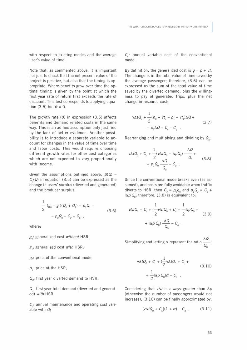
with respect to existing modes and the averageuser’s value of time.

Note that, as commented above, it is importantnot just to check that the net present value of theproject is positive, but also that the timing is ap-propriate. Where benefits grow over time the op-timal timing is given by the point at which thefirst year rate of return first exceeds the rate ofdiscount. This test corresponds to applying equa-tion (3.5) but i = 0.

The growth rate (i) in expression (3.5) affectsbenefits and demand related costs in the sameway. This is an ad hoc assumption only justifiedby the lack of better evidence. Another possi-bility is to introduce a separate variable to ac-count for changes in the value of time over timeand labor costs. This would require choosingdifferent growth rates for other cost categorieswhich are not expected to vary proportionallywith income.

Given the assumptions outlined above, B(Q) –Cq(Q) in equation (3.5) can be expressed as thechange in users’ surplus (diverted and generated)and the producer surplus:

1— (g0 – g1)(Q0 + Q1) + p1Q1 –2 (3.6)

– p0Q0 – Cq + CC ,

where:

g0: generalized cost without HSR;

g1: generalized cost with HSR;

p0: price of the conventional mode;

p1: price of the HSR;

Q0: first year diverted demand to HSR;

Q1: first year total demand (diverted and generat-ed) with HSR;

Cq: annual maintenance and operating cost vari-able with Q;

CC: annual variable cost of the conventionalmode.

By definition, the generalized cost is g = p + vt.The change is in the total value of time saved bythe average passenger; therefore, (3.6) can beexpressed as the sum of the total value of timesaved by the diverted demand, plus the willing-ness to pay of generated trips, plus the netchange in resource cost:

1vΔtQ0 + —(p0 + vt0 – p1 – vt1)ΔQ +

2 (3.7)+ p1ΔQ + Cc – Cq .

Rearranging and multiplying and dividing by Q0:

1 ΔQvΔtQ0 + Cc + —(vΔtQ0 + ΔpQ0) —— +

2ΔQ

Q0 (3.8)+ p1Q0 —— – Cq .

Q0

Since the conventional mode breaks even (as as-sumed), and costs are fully avoidable when trafficdiverts to HSR, then Cc = p0q0 and p1Q0 = Cc +|Δp|Q0; therefore, (3.8) is equivalent to:

1 1vΔtQ0 + Cc + (—vΔtQ0 + Cc + —ΔpQ0 +

2 2 (3.9)

ΔQ+ |Δp|Q0) —— – Cq .

Q0

ΔQSimplifying and letting a represent the ratio ——:

Q0

1vΔtQ0 + Cc + (—vΔtQ0 + Cc +

2 (3.10)1

+ —|Δp|Q0)a – Cq .2

Considering that vΔt is always greater than Δp(otherwise the number of passengers would notincrease), (3.10) can be finally approximated by:

[vΔtQ0 + CC](1 + a) – Cq , (3.11)


63

11 There is also evidence of a systematic bias in the estima-tion of costs and demand in large infrastructure projects.Flyvbjerg, Skamris, and Buhl (2004) found that 90% of

projects have cost overruns. Overruns are general inspace and constant for the past 70 years.

where:

v: average value of time;

Δt: average time saving;

Q0: first year diverted demand to HSR;

CC: annual variable cost of the conventionalmode;

a: proportion of generated passengers with theproject with respect to Q0.

For (3.11) be equivalent to (3.10) it is requiredthat vΔt = |Δp| and, therefore, (3.11) overesti-mates the benefit from generated traffic by thedifference vΔt – |Δp| which, if significant, wouldbias the evaluation in favor of the project.

Substituting (3.11) back in (3.5) and rearrangingit, it is straightforward to figure out the minimumvalue of Q0 , which would be necessary for a pos-itive NPV:

1 r – iQ0 > ————— [ ——————I + Cq +

vΔt(1 + a) 1 – e–(r – i)T

(3.12)r – i 1 – e–rT

+ Ct ——— —————— – CC (1 + a)] .r 1 – e–(r – i)T

3.4.3 DEMAND THRESHOLDS FOR SOCIAL

PROFITABILITY

We have limited information concerning the actu-al values of key parameters in (12). Having aHSR line in operation requires incurring somefixed (and partially sunk) costs: the investmentcosts in infrastructure, which consists of tracksand sidings along the line, buildings and techni-cal equipment for terminals and stations, linesignalling, traffic management and control sys-tem. These components need maintenance andoperation (energy, materials and labor) and a

reservation system; and although these costs arein some way dependent on the volume of traffic,they cannot be completely avoided when demandis lower than expected, and therefore they areconsidered fixed in this chapter.

Besides dedicated infrastructure, investment inhigh speed rolling stock is required, as well asmaintenance and operating costs such as energyand labor expenses needed for having thesetrains in operation. These costs are demand-re-lated but they could be partially considered asfixed in the short term. In this chapter, we willconsider all these costs as variable, i.e., relatedto the level of demand.

It is not easy to obtain cost values for HSR proj-ects because the range of variation is wide, andcosts vary according to local conditions: density ofcrossed urban areas, number of tunnels, bridges,and so forth. We worked with a range of typicalcost values in standard circumstances (based onthe HSR in operation in Europe), and used differ-ent values of time, from several European studiesin the recent past. Then, we applied a sensitivitytest using the most favorable assumptions regard-ing key parameters.

Data on infrastructure construction costs showshow the cost per kilometer varies from €12 mil-lion per kilometer in Spain to 32 in Germany andover 45 in the Netherlands (Department of Envi-ronment, Transport and the Regions 2004). Inspite of the difficulties associated to the limitedevidence concerning cost data, it is possible towork within certain realistic ranges for standardprojects.11 Table 3.7 shows the actual costs for astandard 500-km HSR (see Barrón de Angoiti2004).

The lower value of construction costs in table 3.7is representative of the line Madrid-Seville (Spain)or the TGV Atlantique (France); the highest valuewould reflect the construction costs of lines likeNaples-Rome and Florence-Turin (Italy); in themiddle lie the TGV Méditerenée (France) and the


64

12 These figures underline the importance of the chosenbase case in cost-benefit analysis.

13 Cost savings in conventional modes were found to be

one third of Ct+Cq in the Madrid-Seville evaluation (DeRus and Inglada 1997).

14 See European Commission (1997).

ICE Frankfurt-Cologne (Germany), which is closerto the upper limit.

One key parameter is the expected averagetime saving per passenger (Δt). SDG (2004)provides some evidence from case studies onHSR development, transport markets and ap-praisal processes in the UK and six other coun-tries. The base case is a conventional rail serv-ice with an operating speed of 130 km/h(representative of many main lines in Europe).For distances in the range of 350-400 km, atypical HSR yields 45-50 minutes savings.When conventional trains run at 100 km/h, po-tential time savings are one hour or more. Onthe other hand, if the conventional train’s oper-ating speed is 160 km/h, time saving is 35minutes over a distance of 450 km.12

These average values imply that all passengerstravel the whole length of the line. Given the exis-tence of intermediate stations along the line anddifferent trip lengths, these values overestimatethe actual time savings. Moreover diverted trafficalso comes from road and air transport. Time sav-ings are lower when passengers divert from airtransport, though higher when passengers shiftfrom road transport. In this chapter we assumethat the average time saving per passenger goes

from half an hour to an hour and a half, whichprobably includes any potential case in Europe.

Other key parameters are the value of time andthe social discount rate. We use average values oftime ranging from 15 to 30 euros. For the sake ofrobustness, the maximum value chosen is abovethe state-of-the-art values (see, for example,Nellthorp et al. 2001). This range includes differ-ent possibilities of trip purposes and initial trans-port mode combinations, and the possibility of anextra willingness to pay for quality not included inthe reported values of time. Avoidable costs in theconventional mode (CC) are initially assumed tobe a half of (Ct+Cq) in the high speed train.13 Thesocial discount rate is 5% in real terms, as recom-mended by the European Commission for theevaluation of infrastructure projects.14

Expression (3.12) allows the estimation of de-mand thresholds changing the average time sav-ings, the value of time and other relevant param-eters. Graphs 3.2a to 3.2d represent isoquantsfor particular values of Q that allow a NPV equalto zero. These values correspond to a 500-kmline, an optimal distance for a HSR project. Anyisoquant shows the level of demand required fora positive NPV for different vΔt and investmentcosts (including rolling stock), under alternative


65

TABLE 3.7: Estimated costs of a 500-km HSR line in Europe (2004)

Cost per unit (€ thousand) Units Total cost (€ million)

Capital costs

Infrastructure construction* (Km) 12,000-40,000 500 6,000-20,000

Rolling stock (Trains) 15,000 40 600.0

Running costs (p.a.)

Infrastructure maintenance (Km) 65 500 32.5

Rolling stock maintenance (Trains) 900 40 36.0

Energy (Trains) 892 40 35.7

Labor (Employees) 36 550 19.8

* Terminal value = 50% of the investment in infrastructure.

Source: UIC.


66

scenarios for generated traffic and annual growthof net benefits.

The isoquants can be interpreted in differentways, but one interesting approach is to checkwhich minimum levels of demand are requiredfor a particular range of expected values of in-vestment (rolling stock included) and expectedtotal value of time savings per average passenger.The isoquants in graphs 3.2a to 3.2d show thatfor a 500-km line, even in the best cases of lowinvestment costs, high annual growth of net ben-efits and a high proportion of generated passen-gers, it is difficult to find a case for a HSR invest-ment below a first year demand of at least 6million passengers; in terms of optimal timing,such investment should not be undertaken untiltraffic has grown to somewhat more than that.

Tables 3.8 and 3.9 show a sensitivity test for firstyear demand thresholds leading to an NPV = 0.Investment costs per kilometer are 12, 20, 30,and 40 million euros. The average benefit perpassenger is 20, 30, and 45 euros. The percent-ages of generated demand relative to diverted de-mand are 20, 30, 40, and 50. Annual growth ofnet benefits is 2, 3, and 4%. The social discountrates are 5 and 3% alternatively. These tables re-

inforce the fact that we only find a case for HSRat a total demand below 6 million passengersp.a. in circumstances where low constructioncosts and a low discount rate are combined withhigh values of time savings per passenger. Withhigh construction costs but otherwise favorablecircumstances, a total first year demand of atleast 9 million trips p.a. is needed; in unfavor-able circumstances, the requirement may beconsiderably more than that.

As we stress throughout this chapter, the esti-mated demand thresholds are obtained assumingthat benefits come from time savings of divertedtraffic from competing modes. When the provi-sion of new rail capacity is needed, and there issignificant congestion in roads and airports, ad-ditional benefits of HSR investment will reducethe required first year demand for a positive NPV.The construction of new HSR lines increases ca-pacity for both passengers and freight, both byproviding the new infrastructure itself and by re-leasing capacity in existing routes. In the Britishcase study, these benefits appear to have ac-counted for around 10% of the benefits, whichwill be equivalent to adding 10% to the level ofdemand, so the change they bring is not dramat-ic. In those cases where serious bottlenecks

Note: Qd: diverted demand; Qt: total demand Qt=Qd(1+a); a: proportion of generated traffic; i: annual growth of net benefits; v: average value of time; Δt: averagetime saving per passenger.

0

5

10

15

20

25

30

35

40

7,5 9 10,5 12 13,5 15 16,5 18 19,5 21 22,5 24 25,5 27 28,5 30 31,5 33 34,5 36 37,5 39 40,5 42 43,5 45

First year vΔt (€)

Inve

stm

ent C

ost /

Km

(€ m

illio

n)

Qd = 12 (Qt = 14.4)

Qd = 10 (Qt = 12)

Qd = 8 (Qt =9.6)

Qd = 6 (Qt = 7.2)

a = 0.2i = 3%

Graph 3.2a First year demand required for NPV = 0 (a = 0.2 i = 3%).


67

Graph 3.2b First year demand required for NPV = 0 (a = 0.2 i = 4%).

7,5 9 10,5 12 13,5 15 16,5 18 19,5 21 22,5 24 25,5 27 28,5 30 31,5 33 34,5 36 37,5 39 40,5 42 43,5 45

a = 0.2

i = 4%

0

5

10

15

20

25

30

35

40

45


Inve

stm

ent

Cos

t /

Km

(€ m

illio

n)

Qd = 12 (Qt = 14.4)

Qd = 10 (Qt = 12)

Qd = 8 (Qt =9.6)

Qd = 6 (Qt = 7.2)


Graph 3.2c First year demand required for NPV = 0 (a = 0.4 i = 3%).

0

5

10

15

20

25

30

35

40

45


Inve

stm

ent

Cos

t /

Km

(€ m

illio

n)

a = 0.4

i = 3% Qd = 12 (Qt = 16.8)

Qd = 10 (Qt = 14)

Qd = 8 (Qt = 11.2)

Qd = 6 (Qt = 8.4)

7,5 9 10,5 12 13,5 15 16,5 18 19,5 21 22,5 24 25,5 27 28,5 30 31,5 33 34,5 36 37,5 39 40,5 42 43,5 45



68

Graph 3.2d First year demand required for NPV = 0 (a = 0.4 i = 4%).

0

10

20

30

40

50

60


Inve

stm

ent

Cos

t /

Km

(€

mill

ion)

a = 0.4i = 4%

Qd = 12 (Qt = 16.8)

Qd = 10 (Qt = 14)

Qd = 8 (Qt = 11.2)

Qd = 6 (Qt = 8.4)

7,5 9 10,5 12 13,5 15 16,5 18 19,5 21 22,5 24 25,5 27 28,5 30 31,5 33 34,5 36 37,5 39 40,5 42 43,5 45


TABLE 3.8: First year demand thresholds for NPV=0(r=5% T=40 Ct=32.5 Cq=91.5 Cc=62)

Qt

a

20% 30% 40% 50%

i

2% 3% 4% 2% 3% 4% 2% 3% 4% 2% 3% 4%

I

12

vΔt

20 14.9 12.8 10.8 14.6 12.5 10.5 14.3 12.2 10.2 14.0 11.8 9.9

30 10.0 8.5 7.2 9.8 8.3 7.0 9.5 8.1 6.8 9.3 7.9 6.6

45 6.6 5.7 4.8 6.5 5.5 4.7 6.4 5.4 4.5 6.2 5.3 4.4

20

20 23.5 20.0 16.9 23.2 19.7 16.6 22.9 19.4 16.3 22.6 19.1 15.9

30 15.7 13.4 11.2 15.5 13.2 11.0 15.3 12.9 10.8 15.1 12.7 10.6

45 10.5 8.9 7.5 10.3 8.8 7.4 10.2 8.6 7.2 10.0 8.5 7.1

30

20 34.3 29.1 24.5 33.9 28.8 24.1 33.6 28.5 23.8 33.3 28.2 23.5

30 22.8 19.4 16.3 22.6 19.2 16.1 22.4 19.0 15.9 22.2 18.8 15.7

45 15.2 12.9 10.9 15.1 12.8 10.7 15.0 12.7 10.6 14.8 12.5 10.5

40

20 45.0 38.2 32.0 44.7 37.9 31.7 44.4 37.6 31.4 44.1 37.3 31.1

30 30.0 25.5 21.4 29.8 25.3 21.2 29.6 25.0 20.9 29.4 24.8 20.7

45 20.0 17.0 14.2 19.9 16.8 14.1 19.7 16.7 14.0 19.6 16.6 13.8

Qt: total demand (millions of passenger-trips) a: proportion of generated traffic

i: annual growth rate of net benefits v: average value of time (€/hour)

Δt: average time saving per passenger (hours) I: investment cost per kilometer (construction + NPV of rolling stock, € million)

r: interest rate T: life of the project (years)

Ct: annual fixed maintenance and operating costs (€ million) Cq: annual maintenance and operating cost variable with Q (€ million)

Cc: annual variable cost of the conventional mode (€ million) Cc=1/2(Ct+Cq)

make it very difficult to introduce upgraded ser -vices on existing routes, the case for HSR invest-ment is stronger. The case will also be stronger incircumstances where high speed rail providesmajor environmental benefits or indirect econom-ic benefits.

3.5 CONCLUSIONS

The case for building new High Speed Rail (HSR)infrastructure depends on its capacity to generatesocial benefits which compensate for the con-struction, maintenance and operation costs. Deci-sions to invest in this technology have not alwaysbeen based on sound economic analysis. A mix ofarguments, besides time savings—strategic con-siderations, environmental effects, regional devel-opment, and so forth—has often been used withinadequate evidence to support them.

Whether HSR investment is socially profitabledepends on the local conditions, which deter-mine the magnitude of costs, demand levels andexternal benefits such as reduced congestion orpollution from other modes. Given the costs, theexpected net social benefit of the investment inHSR relies heavily on the number of users and itscomposition (diverted and generated passengers)and the degree of congestion in the corridor af-fected by the investment. HSR projects require ahigh volume of demand with enough economicvalue to compensate for the high cost involved inproviding capacity and maintaining the line. It isnot only that the number of passengers must belarge, a high willingness-to-pay for the new facil-ity is required: many users who obtain high ben-efits when switching to HSR or making more jour-neys.

HSR investment does not only save time but alsoincreases capacity for passengers as well as forfreight, both by providing capacity itself and by


69

TABLE 3.9: First year demand thresholds for NPV=0(r=3% T=40 Ct=32.5 Cq=91.5 Cc=62)

Qt

a

20% 30% 40% 50%

i

2% 3% 4% 2% 3% 4% 2% 3% 4% 2% 3% 4%

I

12

vΔt

20 11.1 10.0 7.7 10.8 9.7 7.4 10.5 9.4 7.1 10.2 9.1 6.8

30 7.4 6.7 5.1 7.2 6.4 4.9 7.0 6.2 4.7 6.8 6.0 4.5

45 4.9 4.4 3.4 4.8 4.3 3.3 4.7 4.2 3.2 4.5 4.0 3.0

20

20 17.2 15.0 11.8 16.9 14.7 11.5 16.5 14.4 11.2 16.2 14.1 10.9

30 11.4 10.0 7.9 11.2 9.8 7.7 11.0 9.6 7.4 10.8 9.4 7.2

45 7.6 6.7 5.2 7.5 6.5 5.1 7.4 6.4 5.0 7.2 6.2 4.8

30

20 24.8 21.2 16.9 24.4 20.9 16.6 24.1 20.6 16.3 23.8 20.3 15.9

30 16.5 14.2 11.2 16.3 13.9 11.0 16.1 13.7 10.8 15.9 13.5 10.6

45 11.0 9.4 7.5 10.9 9.3 7.4 10.7 9.2 7.2 10.6 9.0 7.1

40

20 32.3 27.5 22.0 32.0 27.2 21.6 31.7 26.9 21.3 31.4 26.6 21.0

30 21.6 18.3 14.6 21.4 18.1 14.4 21.1 17.9 14.2 20.9 17.7 14.0

45 14.4 12.2 9.8 14.2 12.1 9.6 14.1 11.9 9.5 14.0 11.8 9.3

Qt: total demand (millions of passenger-trips) a: proportion of generated traffic

i: annual growth rate of net benefits v: average value of time (€/hour)

Δt: average time saving per passenger (hours) I: investment cost per kilometer (construction + NPV of rolling stock, € million)

r: interest rate T: life of the project (years)

Ct: annual fixed maintenance and operating costs (€ million) Cq: annual maintenance and operating cost variable with Q (€ million)

Cc: annual variable cost of the conventional mode (€ million) Cc=1/2(Ct+Cq)

releasing capacity on existing routes. In thoseroutes characterized by serious bottlenecks, theopportunity to upgrade the existing services is afactor which may well increase the added valueof HSR.

We explored under what conditions net welfaregains can be expected from new HSR projects. Inthis chapter, we use some simplifying assump-tions with the aim of obtaining a benchmark: theminimum level of demand from which a positivesocial net present value could be expected whennew capacity does not provide additional benefitsbeyond time savings from diverted and generateddemand.

It appears that only under exceptional circum-stances (a combination of low construction costsplus high time savings, perhaps because the ex-isting rail infrastructure and services on compet-ing modes are very poor) could a new HSR line bejustified with a level of patronage below 6 millionpassengers per annum on opening; with moretypical construction costs and time savings a fig-ure more like 9 million passengers per annum isneeded.

Judging from the British example, allowing forthe release of capacity on existing lines may onlyreduce this figure by some 10%; allowing for op-timal timing may increase it. Of course in a net-work, individual links may be justified with lowerlevels of demand, provided that the increase intraffic density on the network as a whole pro-duces an equivalent additional traffic volume.

Also the demand thresholds reported in thischapter assume benefits grow in the same orderas GDP. Where there is both underlying growth indemand and growth in the value of time savings,it may understate benefit growth. Significant en-vironmental or indirect economic benefits wouldalso strengthen the case, but it appears that—when allowance is made for the increased envi-ronmental costs of trips diverting from conven-tional rail—net environmental benefits may besomewhat marginal, whilst indirect economicbenefits are both highly variable and uncertain.

Our results suggest that, given typical rail de-mand volumes in Europe, investment in HSR in-frastructure on a single corridor can rarely be jus-tified on the basis of time savings and the netwillingness to pay of generated traffic alone. In-stead the investment could be justified by a com-bination of factors: the need to bypass bottlenecksections, the existence of network benefits aris-ing from serving a variety of traffic flows with asingle link, and the presence of congestion or en-vironmental problems in competing transportmodes. These are indeed features of much of theFrench and German high speed networks and ofproposals for Britain but are less likely to befound in countries with lower population densityaway from the core of Europe.


Chris NashUniversity of Leeds


70

1 These are well-known results in transport demand litera-ture involving modal choice. An extensive and specific

survey of intermodal demand modelling related to highspeed rail can be found in chapter 3 of COST318 (1998).

4.1 INTRODUCTION

From the point of view of the transport system asa whole, High Speed Rail (HSR) may act as asubstitute or as a complement of other transportmodes. It acts as a competitor when provides al-ternative transport services in the same point-to-point market already served by air companies,(private or public) road transport, maritime ser -vices (such as in the Channel Tunnel) or evenconventional rail services. On the other hand,HSR complements other modes when it en-hances intermodal transport at interchange in-frastructure (airports, ports, bus stations), be-having as a feeder/receiver for/from transfermarkets (at regional or urban levels) not coveredby HSR. However although both roles becomecrucial when evaluating the overall economicimpact of this technology, a larger part of the ex-isting literature has generally focused on thecompetitive edge of HSR (Pavaux 1991).

On any given city-pair corridor, most of the rela-tive advantage of high speed rail services is tradi-tionally attributed to its lower travel time, whichfavors direct journeys over medium distances,whereas larger journeys tend to be dominated byair transport, and shorter ones are mostly carriedout by road or conventional rail. When the journeyinvolves more than one mode, the choice of HSRcritically depends on its integration within theoverall transport system.1 However, as pointed outin SDG (2004), «the exact range of journeys overwhich high speed rail is competitive (…) clearly

varies depending on assumptions about time re-quired for station and airport access, check in,etc.» As a consequence, it may be deduced thatthe market advantage of HSR and, presumably, itseffects on other transport modes also varies withall the components of the generalized cost forpassengers (the relative price of transport, thequality and reliability of other modes, and the in-tegration of HSR within the transport system)which are particular to specific routes.

The empirical evidence accumulated after morethan 30 years of operation of high speed lines(25 years in Europe) should suffice to provide acomplete analysis of the true determinant of theintermodal effects of HSR. However, apart fromsome seminal contributions (e.g., Nash 1991),the published experiences that have attemptedto provide an integrated framework to explain theintermodal effects of HSR are relatively scarce(as compared to what might be expected), most-ly due to two main reasons: firstly, operators andgovernments are mostly interested in the ex-anteresearch to justify these expensive schemes butseem to lose interest in the evaluation of theproject once it has been constructed, and sec-ondly, the research findings are often commer-cially confidential, particularly in Europe, sinceit is expected that national rail markets will beopen to competition in the near future.

Although this gap has been filled during the lastyears, the recent empirical literature analyzingintermodal effects of HSR is dominated by the

71

4

Measuring the Intermodal Effects

of High Speed Rail

papers by López-Pita (2001a, 2001b), López-Pita and Robusté (2003, 2005) and López-Pitaet al. (2006), which provide a detailed technicalstudy of the impact of high speed rail on othermodes in terms of market shares for the most rel-evant corridors. Janic (1993, 2003) comparesthe operational performance of HSR and air passen-ger transport across several countries, insistingon their substitute vs. complement roles. Levin-son et al. (1997) analyze the San Francisco-LosAngeles corridor providing costs estimates for apotential high speed service. At the Europeanlevel, the most comprehensive official documentso far is the COST318 (1998) study, which dis-cusses several case studies on the interaction be-tween high speed and air passenger transport.Park and Ha (2006) analyze the Korean case,whereas González-Savignat (2004) is one of thefew papers that specifically focuses on the com-petition between HSR and private transport.More recent works have modelled the relation-ship between HSR on one hand, and traditionalor low-cost airlines on the other, as in Friebel andNiffka (2005) for Germany, Ivaldi and Vibes(2005), Crisalli et al. (2007) or Adler, Nash, andPels (2007). Still, the most data-extensive studyon this issue was carried out by the UIC (2003),analyzing the influence of low-cost air companiesand long-distance coaches on the demand ofpassenger rail services in several European corri-dors. Finally, Martín and Nombela (2007) pro-vide intermodal share estimations for Spain inthe 2010-horizon.

The objective of this chapter is to contribute tothis growing literature by providing a formal ap-proach that could clarify some of the determi-nants that explain the intermodal effects of HSR.For that reason, our contribution is twofold. First,after this introduction, we summarize some ofthe most relevant empirical findings related tothe intermodal effects of HSR worldwide, discussthe substitute/complement role of high speedand analyze, through examples from the existingroutes, the current situation in several countries.Then, in section 4.3, we provide a theoreticalmodel that could be viewed as a methodologicalapproach to be used for carrying out this sort ofintermodal analysis. The model proceeds as fol-lows: in a first step, as in Ivaldi and Vibes(2005), travellers choose a transport mode and

an operator to travel on a route between an originand a destination, which is modelled as a marketwith differentiated services competing againsteach other. Second, on the supply side, we en-dogenize the costs of the transport operators,thus accounting for the various competitivepressures impinging on their activity, dependingon the type of route they operate. Section 4.4explains how this model could be solved and em-pirically implemented, the data requirementsand the limitations it could face. Section 4.5proposes a simulation exercise where operators’own-price demand elasticities as well as margin-al costs and margins are evaluated. We showhow this exercise can be implemented with verylittle data, and we suggest that, on the very spe-cific route we consider as example (the Paris-Amsterdam line), and when compared with oth-er competing transport modes, HSR faces theless elastic demand curve and enjoys the high-est price-cost margins. Section 4.6 is finally de-voted to conclusions.

4.2 INTERMODAL EFFECTS OF HSR:

A SUMMARY OF EMPIRICAL FINDINGS

When choosing among alternative transportmodes, rational passengers make their deci-sions by comparing the generalized cost ofeach mode. This cost includes not only the fareand other monetary costs, but also total traveltime, and many other factors related to the per-ceived quality of the service (such as reliabili-ty, comfort, amenities, safety, etc.) (see Quinetand Vickermann 2004). From a broader per-spective, and when the journey involves morethan one mode, integration within the overalltransport system may also affect the perceivedquality of each mode, and thus, the modalchoice. Rail terminals, for example, are oftenwell located in terms of accessibility to citycenters and densely populated areas, whereasairports tend to be on the outskirts of cities,with worse accessibility. Rail is also in astronger position when serving large conurba-tions, and demand levels are sufficiently highto warrant frequent services.


72

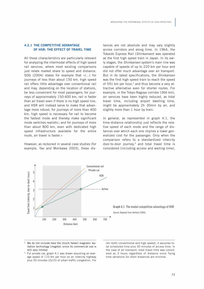
2 We do not include here the (much faster) magnetic lev-itation technology (maglev), since its commercial use isstill very limited.

3 For private car, graph 4.1 was drawn assuming an aver-age speed of 110 km per hour on an intercity highwayplus 30 minutes (2x15) of urban traffic congestion. For

rail (both conventional and high speed), it assumes to-tal scheduled time plus 30 minutes of access time. Inthe case of air transport, total travel time was consid-ered as 3 hours regardless of distance since flyingtime variations for short distances are minimal.

4.2.1 THE COMPETITIVE ADVANTAGE

OF HSR: THE EFFECT OF TRAVEL TIME

All these characteristics are particularly relevantfor analyzing the intermodal effects of high speedrail services, where most existing comparisonsjust relate market share to speed and distance.SDG (2004) states for example that «(...) forjourneys of less than about 150 km, high speedrail offers little advantage over conventional railand may, depending on the location of stations,be less convenient for most passengers; for jour-neys of approximately 150-400 km, rail is fasterthan air travel even if there is no high speed line,and HSR will instead serve to make that advan-tage more robust; for journeys of more than 400km, high speed is necessary for rail to becomethe fastest mode and thereby make significantmode switches realistic; and for journeys of morethan about 800 km, even with dedicated highspeed infrastructure available for the entireroute, air travel is faster.»

However, as reckoned in several case studies (forexample, Yao and Morikawa 2003), these dis-

tances are not absolute and may vary slightlyacross corridors and along time. In 1964, theTokaido Express Rail (Shinkansen) was operatedas the first high speed train in Japan. In its ear-ly stages, the Shinkansen system’s main line wascapable of speeds of up to 220 km per hour anddid not offer much advantage over air transport.But in its latest specifications, the Shinkansenwas the first high speed train to reach the speedof 591 km per hour,2 and thus become a very at-tractive alternative even for shorter routes. Forexample, in the Tokyo-Nagoya corridor (366 km),air services have been highly reduced, as totaltravel time, including airport dwelling time,might be approximately 2h 30min by air, andslightly more than 1 hour by train.

In general, as represented in graph 4.1, thetime-distance relationship just reflects the rela-tive speed of each mode and the range of dis-tances over which each one implies a lower gen-eralized cost for the passenger. Only when thecomparison refers to a standardized intercitydoor-to-door journey,3 and total travel time isconsidered (including access and waiting time),

MEASURING THE INTERMODAL EFFECTS OF HIGH SPEED RAIL

73

Conventional rail

5

4

3

2

1

100 200 300 400 500 600 700

Trav

el t

ime

(int

erci

ty, d

oor-

to-d

oor)

(hou

rs)

Distance (km)

Airline

HSR

Private car

Graph 4.1 The modal competitive advantage of HSR

Source: Adapted from Sellnick (2006).

4 Other factors, such as network configuration, conges-tion, etc. may affect the relative generalized costs (see

De Rus, Campos, and Nombela 2003).

it can be safely said that HSR has a competitiveadvantage (the shaded area) only for mediumdistance journeys, in the range of 100-500 km,depending on the corridor.4 In general, it is verydifficult for air transport services to compete ef-fectively in the short-haul transport marketagainst other modes. In the 500 km-plus long-haul transport market, however, most air trans-port services can successfully compete with highspeed rail.

Travel time is indeed the key factor explaining railvs. air modal share in most existing studies thathave empirically examined the intermodal effectsof high speed rail. Table 4.1 summarizes some ofthe most recent findings showing that, in general,where the high speed train offers a journey timeof three hours or less, it captures at least 60% ofthe combined rail and air market. Conversely, thisshare goes down very sharply as journey time in-creases beyond three hours.

In all the corridors in the table, the effect of to-tal journey time on rail share closely follows thepattern drawn in graph 4.1, although perhaps theBrussels-London route might be expected toachieve a higher share and the Paris-Amsterdamroute a lower share. The strength of air competi-tion on the first route and the weakness of thatsame competition in the second one may explainthese results. It is also noticeable that rail hascaptured virtually the entire market on the Paris-Brussels route and, in fact, there is very little airactivity between these two airports.

Table 4.1 shows that rail market share is not al-ways a linear function of absolute travel time.Other studies have focused instead in travel timedifferences with respect to air competitors. Thisapproach is particularly useful for analyzing theimpact of HSR over different passenger seg-ments. In COST318 (1998) it is stated, for exam-ple, that «business travellers will hardly considerthe rail alternative over medium distances if itcannot accommodate the trip in a single day whenair can.» This requires a round trip journey timeof less than six hours and a minimal difference in

access and waiting times. In France, where railhas become very competitive with air in manyHSR corridors, the public operator SNCF official-ly aims at attracting around half of the businesspassenger market. On average, in 2002-2005, itconsolidated a market share (with respect to air)of 19% in «professional trips» plus 7% in «otherprivate trips, not leisure» (Bernard 2006).

From the point of view of airlines, they reckonthat the adverse impact of HSR services is initial-ly severe and often increases during the following2-5 years. For example, COST318 (1998) assertsthat the introduction of the AVE between Madridand Seville (471 km) in 1992 reduced in sixmonths the number of weekly flights from 71 to40, and the airlines lost more than 20% of mar-ket share in one year. The Paris-Lyon south-eastroute (450 km) was opened in 1981 as the veryfirst route of the TGV, and immediately had a sig-nificant intermodal impact. By 1997, once otherhigh speed routes had been also introduced, air -lines’ share in domestic passenger transport mar-kets had decreased by almost half, from 30% to16%, especially in medium distance routes (aspredicted in graph 4.1). In some longer routes theimpact after three years of HSR services was alsosignificant: in the Paris-Marseille corridor (700km), the air transport share dropped from 45-55%


74

TABLE 4.1: Travel time and rail market share on selectedcorridors

Corridor (km) Year Travel time Rail share (*)

Tokyo-Osaka (515) 2005 2h 30min 81%

Tokyo-Okayama (643) 2005 3h 16min 57%

Tokyo-Hiroshima (814) 2005 3h 51min 47%

Tokyo-Fukuoka (1069) 2005 4h 59min 9%

Paris-London (257) 2005 2h 40min 66%

Paris-Amsterdam (514) 2004 4h 10min 45%

Brussels-London (204) 2005 2h 20min 60%

Paris-Geneva (339) 2003 3h 30min 35%

Paris-Brussels (183) 2006 1h 25min 100%

* Rail market share was calculated with respect to the combined air-rail market.

Source: Adapted from López-Pita et al. (2006).

to 35-45%, and in the Paris-Nice route (900 km)it fell from 55-65% to figures around 50-60%.

In the longer run, it has been argued that this re-trenchment by the airlines, as well as having en-vironmental and congestion benefits at airports,will tend to reinforce the rail demand effect.Wilken (2000) points out that in France the in-troduction of HSR caused a sharp reduction inthe number of regional flights, and there was alsoa movement towards smaller planes. In the twoyears after HSR introduction in the Paris-Lyoncorridor, the change in aircraft movements be-tween their airports was only 0.53% per year,compared to a 9.3% increase per year betweenParis and Bordeaux, which at the time had nohigh speed services.

Another example corresponds to the Paris-Londoncorridor, where trains are winning the competitionagainst aircrafts. By August 2004, the HSR hadcaptured 68% of this market (Givoni 2005), al-though the airlines continued to offer about 60flights a day between Heathrow and Charles deGaulle airports. In general, although the airlinesare likely to lose from this competition, they willnot exit the market if such routes are important atthe network level and are used to feed traffic intothe more profitable (mainly long-haul) routes.Other alternative will be the low-cost and charterflights segments, which can possibly competemore advantageously with HSR.

With respect to the effects of the introduction ofHSR on road and conventional rail market shares,the comparable evidence across countries is morelimited due to the lack of accurate passenger trav-el statistics of road users. In general, as showedby table 4.2, the impact of high speed trains onconventional services in Europe, after a decade ofintermodal competition, was almost definitive: onaverage their share fell below 4%, partly becausemany of them were just suppressed on overlap-ping corridors, and partly because most of themwere used only by low-income passengers thatcould not afford or were not willing to pay for aseat on HSR services. The change in the roadmarket share was less impressive but significantin all three examples depicted in the table. As inthe case of air transport, it was heavily dependenton the amount of travel time reduction, as gener-

ally predicted by several empirical studies (seeGonzález-Savignat 2004, for example).

Finally in Japan and Korea, a large part of theHSR share in many corridors was stolen fromroad transport. Yao and Morikawa (2003) sug-gest that the increase in speed and frequenciesin HSR services during the last decade has ledto a reduction of at least 10% in the number ofbus travellers nationwide for distances below500 km. Park and Ha (2006) reports a reduc-tion of 18-25% in express bus services twoyears after the introduction of HSR betweenSeoul and the cities of Deagu and Busan. Inboth countries the impact of high speed trainson air travel was also relevant, but not as largeas in Europe.

4.2.2 THE COMPETITIVE PRESSURE

OF OTHER MODES:

THE EFFECT OF PRICES

Although HSR competitive position against othermodes is basically determined by travel time, it isalso affected by other components of the general-ized cost, which together define the attractive-


75

TABLE 4.2: Modal market share before and after HSR(selected routes)

Paris-Lyon Before HSR (1980) After HSR (1997)

Road 29% 21%

Rail 40% 3%

HSR 0% 70%

Air 31% 6%

Madrid-Seville Before HSR (1991) After HSR (2002)

Road 44% 30%

Rail 16% 1%

HSR 0% 61%

Air 40% 8%

Hamburg-Frankfurt Before HSR (1985) After HSR (2000)

Road 57% 45%

Rail 23% 3%

HSR 0% 48%

Air 10% 4%

* Road combines bus and private car passenger transport; Rail is conventional rail.

Source: Adapted from Gallois (2005) and López-Pita et al. (2006).

ness and availability of a rail service in compari-son to a rival air service on a particular corridor.

In most European countries, high speed rail ser -vices are publicized not only in terms of attrac-tive fares, but also in terms of higher reliability(even with punctuality compromises) and greatercomfort (on-board amenities, distance betweenseats, etc.). Table 4.3 shows, for example, thatthe ratio of airfares over railfares for comparabletariffs over selected corridors always favored therail, which is on average almost 50% cheaper.

The emergence of low-cost airlines in Europeduring the last five years was initially seen as aserious threat to the price advantage of rail ser -vices, particularly in the leisure market. Howev-er, according to an empirical study carried out bythe UIC (2003), most of the risk is limited toconventional rail services, whereas competitionwith HSR services is restricted to a few corridorsin France and Germany. This latter result was re-cently confirmed by Friebel and Niffka, (2005),who also point out that most of the low-cost air-lines’ market share is stolen from conventionalairlines. Furthermore, some rail companies havelearned to react to this menace by launchingtheir own low-cost services, with fewer on-boardservices and a greater focus on the price.

With respect to frequency, its increase has beenlong identified as one of the best strategies ofrailroads against alternative transport modes. Inmost cases, the control of infrastructure andoverall traffic planning by the railways allowsthem (in contrast to most airlines in airports) toadapt their schedules more easily to changingdemand conditions. Leboeuf (2006) says that,under no congestion conditions, high speed

trains are apt to be operated like shuttles. InJapan, for example, the timetable on main linesis based on departures every 4 to 12 minutesfrom 6 a.m. to 11 p.m. In most European HSRcorridors there are more than 25 services perday, an advantage rarely matched by air com-petitors due to airport capacity limits and airtraffic congestion.

4.2.3 THE GROWING ROLE OF HSR

AS A COMPLEMENT TO OTHER

TRANSPORT MODES

Although this is a topic that is just emerging inthe literature and, so far, has not been formallyconsidered in detail, a final element that coulddetermine the effects of HSR on other transportmodes is the degree of intermodality it allows. Aspointed out by López-Pita and Robusté (2003),the collaboration between the railways and theplane with respect to airport access goes back tothe 1950s with the establishment of rail links tofacilitate travel by this mode of transport to air-ports. But the idea of complementarity betweenair services and high speed trains at airports ismuch more recent, dating back to 1985, whenthe French government decided to build the In-terconnection high speed line linking the TGV-South-East, TGV-Atlantic, and TGV-North lines inthe Paris suburbs since it was also intended toserve Charles de Gaulle airport. This first highspeed station entered commercial service in No-vember 1994.

From the viewpoint of users, HSR and air trans-port services are complementary if the combina-tion instead of a single transport mode is pre-ferred for travelling between two cities. Fromthe viewpoint of transport operators, HSR is acomplement to air transport if it replaces short-haul feeder flights connecting into and out oflong-haul flights by using feeder trains accord-ing to a compatible (balanced) timetable. Gen-erally, the literature identifies three types ofcomplementary networks, if commercially vi-able, that may exist:

1) HSR may partially replace air transport in col-lecting and distributing passenger flows be-tween a hub airport and particular spokes. One


76

TABLE 4.3: Airfares vs. HSR fares on selected Europeancorridors

Ratio: Airfare / RailfareBusiness

(First class)Non-business

(Second class)

Paris-Marseille 1.77 2.63

Madrid-Seville 1.29 1.81

Frankfurt-Hamburg 1.43 2.17

Rome-Milan 2.32 2.00

Source: Adapted from López-Pita and Robusté (2005) and Leboeuf (2006).

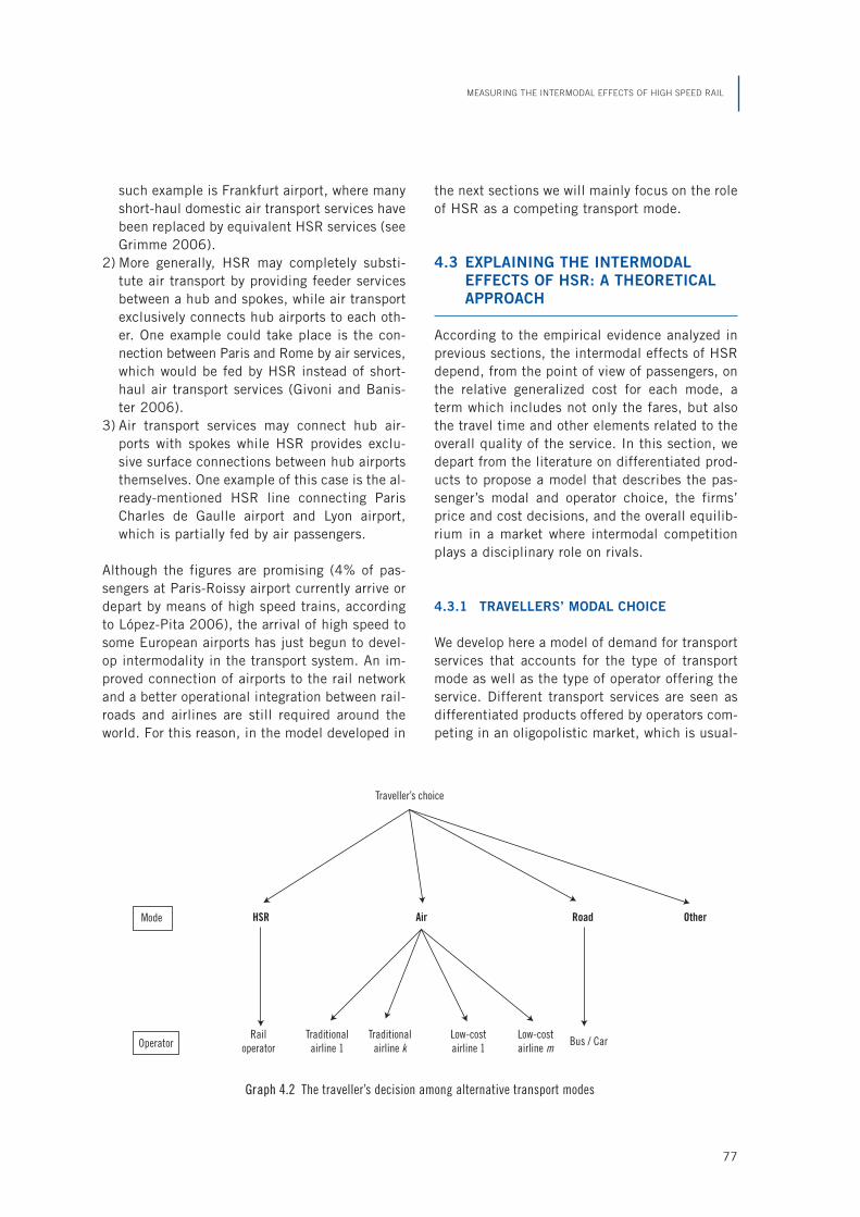
such example is Frankfurt airport, where manyshort-haul domestic air transport services havebeen replaced by equivalent HSR services (seeGrimme 2006).

2) More generally, HSR may completely substi-tute air transport by providing feeder servicesbetween a hub and spokes, while air transportexclusively connects hub airports to each oth-er. One example could take place is the con-nection between Paris and Rome by air services,which would be fed by HSR instead of short-haul air transport services (Givoni and Banis-ter 2006).

3) Air transport services may connect hub air-ports with spokes while HSR provides exclu-sive surface connections between hub airportsthemselves. One example of this case is the al-ready-mentioned HSR line connecting ParisCharles de Gaulle airport and Lyon airport,which is partially fed by air passengers.

Although the figures are promising (4% of pas-sengers at Paris-Roissy airport currently arrive ordepart by means of high speed trains, accordingto López-Pita 2006), the arrival of high speed tosome European airports has just begun to devel-op intermodality in the transport system. An im-proved connection of airports to the rail networkand a better operational integration between rail-roads and airlines are still required around theworld. For this reason, in the model developed in

the next sections we will mainly focus on the roleof HSR as a competing transport mode.

4.3 EXPLAINING THE INTERMODAL

EFFECTS OF HSR: A THEORETICAL

APPROACH

According to the empirical evidence analyzed inprevious sections, the intermodal effects of HSRdepend, from the point of view of passengers, onthe relative generalized cost for each mode, aterm which includes not only the fares, but alsothe travel time and other elements related to theoverall quality of the service. In this section, wedepart from the literature on differentiated prod-ucts to propose a model that describes the pas-senger’s modal and operator choice, the firms’price and cost decisions, and the overall equilib-rium in a market where intermodal competitionplays a disciplinary role on rivals.

4.3.1 TRAVELLERS’ MODAL CHOICE

We develop here a model of demand for transportservices that accounts for the type of transportmode as well as the type of operator offering theservice. Different transport services are seen asdifferentiated products offered by operators com-peting in an oligopolistic market, which is usual-


77

Graph 4.2 The traveller’s decision among alternative transport modes

Traveller’s choice

Mode

OperatorRail

operatorBus / Car

Traditional

airline 1

Traditional

airline kLow-cost

airline 1

Low-cost

airline m

HSR Air Road Other

ly a route between two cities. According to whatwas described in previous sections, transportservices are differentiated in several dimensionscomposing the generalized price, which includes:(1) travel time, (2) fare, and (3) various qualityvariables such as the comfort and amenability,onboard services and extras, ease of interconnec-tion, service on board, whether the service is di-rect or not, etc.

The chain of decisions made by a representativetraveller at the moment of choosing a transportoperator is presented in graph 4.2. First the indi-vidual chooses among the set of transportationmodes, which includes air transportation, highspeed rail, private car, or an alternative decision.Note that the alternative decision may be to trav-el with conventional rail or not to travel at all. Ina second step, the traveller may choose a specif-ic operator inside a transportation mode. The airtransportation set includes traditional airline op-erators as well as low-cost airlines.

This particular decision tree, standard in trans-port demand literature since McFadden (1975),suits perfectly to our integrated approach to theintermodal effects of HSR transport. Dependingon which route is considered, we could as wellconsider an additional decision node inside theairline transportation set, where travellers choosebetween traditional and low-cost airlines, andthen choose the type of operator they want totravel with. This may be potentially relevant onroutes where the share of business travellers ishigh, as these passengers are particularly sensi-tive to the quality of service offered on board.Since considering a three-step decision proce-dure would complicate significantly the exposi-tion, and since its relevance is strongly depen-dant on the type of data available, we leave thispossibility for further research.

Our theoretical analysis departs from a precisedefinition of the utility of the transport user. It isinspired by the literature on differentiated prod-ucts and oligopolistic markets. In particular, thespecification closely follows the exposition of thenested logit model in Berry (1994), and the inter-modal competition model of Ivaldi and Vibes(2005). The key elements of the travellers’ utilityare the characteristics of the transport services

they choose as well as the travellers’ preferences.All characteristics and preferences are assumedto be observed by the participants in the marketbut are not necessarily observed by an externalanalyst. The researcher only observes the marketoutcomes of prices and quantities sold by eachfirm, as well as other service characteristics.

We group the transport decisions j into G + 1 ex-haustive and mutually exclusive sets, whereg = 0, 1,…, G. Thus a decision consists in trav-elling from origin to destination for instance witha particular low-cost carrier, while a transport setwould be for instance air transportation. The out-side decision, j = 0, is assumed to be the onlymember of group 0. The utility of traveller i fortransport service j depends on the characteristicsof the service and the traveller’s. We can denotethis utility as

U(xj, pj, pj, gig, fij ) . (4.1)

The variables in the utility function are as fol-lows: xj and pj denote, respectively, observed andunobserved (by the researcher) service character-istics. Observed characteristics include those de-scribed above (i.e., travel time and quality vari-ables); unobserved ones are those that may bespecific to one particular operator, and that can-not be systematically measured or observed; pj isthe vector of prices; gig and fij are random vari-ables reflecting individual i’s deviation from themean valuation; the term gig is traveller’s i utility,common to all services belonging to group g,whereas the term fij is traveller’s i’s utility, spe-cific to transport service j.

For ease in exposition, we assume that the utili-ty in (4.1) can be rewritten linearly as

uij = dj + gig + (1 – v)fij , (4.2)

where the first term, dj, is the mean valuation forservice j, common to all travellers. It depends onthe price of service j, pj, its observed character-istics, xj, and its unobserved characteristics, pj:

dj = xjb – apj + pj . (4.3)


78

Note that a and b are parameters to be estimated.A third parameter to estimate, 0 ≤ v ≤ 1, deservesadditional explanations. It measures the correla-tion of the travellers’ utility across transport ser -vices belonging to the same group. If v = 1, thereis perfect correlation of preferences for servicesbelonging to the same group. In this case, prod-ucts are perceived as perfect substitutes. As v de-creases, the correlation of preferences for serviceswithin the same group decreases. If v = 0, thereis no correlation of preferences; travellers areequally likely to switch to services in a differentgroup as to services in the same group in responseto a price increase. Thus this framework allowsmodelling correlation between groups of similarservices in a simple way.

Each traveller chooses the service j that maxi-mizes his/her utility. In particular, a travellerchooses a travel alternative j from group g only ifuij > uij' , ∀ j ' = j. If we assume that the expres-sion gig + (1 – v)fij follows an extreme value distri-bution, we can write the market share of servicej inside the total group g as

sj/g = exp(dj /(1 – v))/Dg , (4.4)

where Dg can be written as

Dg = R exp (dj /(1 – v)) , (4.5)jdGg

Similarly the probability of choosing one of thegroup g services is

Dg1–v

sg = ————— . (4.6)

RDg1–v

g

Hence we can write the absolute market share ofservice j as

exp (dj /(1 – v))sj = sj/gsg = ———————— . (4.7)

Dgv RDg

1–v

g

Assuming that the mean utility of the outsidetravel decision is 0, i.e., d0=0, and that this ser -

vice is the only member of group zero, i.e., D0 =1,the market share of the outside travel service isthen

1s0 = ———— . (4.8)

RDg1–v

g

To make this model amenable to the data, a prac-tical procedure suggested by Berry (1994) pro-ceeds as follows: taking the logs of the marketshares sj and s0 as well as the group share sg in(4.7), (4.8), and (4.6) respectively, and substi-tuting, we obtain the following expression thatcan be directly estimated:

ln (sj) – ln (s0) = xjb – apj + vlnsj/g + gj . (4.9)

An estimation of α, b, and v can be obtained us-ing a simple linear regression of the difference inlog market shares on services characteristics andthe log of the within group share. Note that sharescan be obtained as sj = qj /q, and sj/g = qj /qg,where qj is the demand of service j in the market,while q denotes the total size of the market, andqg is the size of the segment g. Note also that de-mand can be measured directly as the number oftravellers, or the number of travellers-kilometerscarried. Finally note that the within group share,sj/g is potentially endogenous, suggesting theneed for additional exogenous variables that arecorrelated with the group share.

4.3.2 TRANSPORT OPERATORS’ PROFITS

Let us now turn to the supply side. Since we havealready seen how travellers make their optimaltravel decision, we need to define how transportoperators behave, that is, how they maximizetheir profit to determine their optimal pricingrule. We will thus obtain a simple economic rulethat ties transport fares to operators’ marginalcosts, depending on demand elasticity.

Before entering into these details, we need to in-troduce the operators’ cost function. We will as-sume that transport operators may face differentincentives to reduce operating costs, dependingon the degree of competition they face. Considerfor instance a route that is operated by a HSR op-


79

5 The way we incorporate the technical inefficiency andeffort parameters allows the incentive-pricing dichoto-my principle to hold (Laffont and Tirole 1993). This

means that the same pricing formula applies whetherwe assume strong or weak competitive pressures.

erator and several airlines (traditional and/or low-cost). The HSR operator competes against groupg operators, while an airline of group g competesat the same time against the HSR operator aswell as the other airlines. We therefore considerthat a transport operator is given higher incen-tives to reduce operating costs and improve itstechnology if more operators of the same type(group) are present on the same route. This canbe accounted for through the structure of thecost function.

4.3.2.1 The primal cost function

To produce a volume of service qj, firm j requiresquantities of labor, lj, materials, mj, and capital,kj. Denote as wl, wm, and wk, the price of labor,materials and capital, respectively. Also denoteby cj the observed operating cost of firm j. An im-portant feature of our model is that the actual op-erating cost may differ from the minimum oper-ating cost. Inefficiency may prevent operatorsfrom reaching the required output level qj at theminimum cost, and this may result in upwarddistorted costs. Firms can also undertake cost re-ducing activities to counterbalance their ineffi-ciency. They can engage in process research anddevelopment; managers may spend time and ef-fort in improving the location of inputs within thenetwork. They can as well attempt to find cheap-er suppliers, bargain better procurement con-tracts, subcontract non-essential activities, mon-itor employees, solve potential conflicts, etc.Whatever these cost reducing activities may be,we will refer to them as effort. Denote by ij andej firm j’s inefficiency and effort levels, respec-tively. Note that these two variables are unob-servable.

Each operator faces a long-run cost function,conditional on inefficiency and effort, of theform:

Cj (qj, wj, zj | ej, ij, ~) , (4.10)

where zj is a vector of service characteristics thataffects operating costs, and ω is a vector of pa-rameters to be estimated. Note that zj may in-clude the vector xj, i.e., the service characteris-tics affecting travellers’ demand may also affectoperating costs. In transport economics, the usu-al variables used by econometricians to capturethe observable heterogeneity across operators’costs include variables such as the size of the op-erator’s network, and the average stage length. Ingeneral, which variables will enter vectors xj andzj depends on data availability. Note also thatwhile inefficiency ij is exogenous, cost reducingeffort ej is a choice variable for firm j, and willtherefore depend on the competitive pressuresimpinging on the activity of the firm.

We describe now the firms’ pricing and effort de-cisions. Before entering into the analysis, it isworth reminding that the pricing structure itselfis independent of the nature of the competitivepressures impinging on the activity of the firm.5

Thus although prices and effort are determinedsimultaneously, the firms’ decisions will be pre-sented separately, for ease of exposition.

4.3.2.2 Competitive pressure and cost reduction

This section focuses on the construction of thestructural cost function. We propose to accountfor the competitive pressures impinging on theoperators’ incentives to reduce costs through thecost function (4.10) that is conditional on ineffi-ciency ij and the effort level ej. Deriving the equi-librium level of effort and plugging it back intothe conditional cost function allows us to derivea structural cost function that can be estimated.The aim of this approach is twofold. First, we cantest whether the different transport operators areinvolved in different cost reduction activities, de-pending on which transport mode they operate,as well as the degree of competitive pressure in-side the particular market (route) they operate.Second, accounting for these changes in incen-


80

6 This assumption is justifiable given that what matters inour analysis is the difference ej

C – ejM. Note that we

do not force ejM to be positive when estimating it.

tives through the cost structure enables us to re-duce the source of misspecification, and avoidbiases in the estimation of the technological pa-rameters.

As mentioned before, a firm can exert effort ej toreduce its operating cost cj. The cost reductionactivity induces an internal cost }(ej | n) wheren is a parameter to be estimated. Taking intoconsideration the operating cost reduction andthe internal cost of effort, the operator sets theoptimal effort level ej that maximizes its profit.Firm j’s profit is the difference between revenueRj = pj qj(·) and total cost cj (ej,.) + }(ej | n):

rj (xj, pj, wj, zj, H) = pjqj (xj, pj, pj, d) –(4.11)

– cj (qj, wj, zj | ej, ij, ~) – }(ej | n) ,

where H = (d, ~, n) is a vector of parameters tobe estimated, and z = (pj, ij, ej) is a vector of un-observable (by the econometrician) variables tobe evaluated.

Each operator j determines the optimal effort lev-el ej that maximizes its profit in (4.11). The firstorder condition is:

∂cj (qj, wj, zj | ej, ij, ~)– ——————————— = }l(ej | n) , , (4.12)

∂e

which implies that the optimal effort level is at-tained by equating the marginal cost reductionand the marginal disutility of effort.

We now consider two competitive situations. First asituation M which refers to a situation where an op-erator is a monopolist inside its group g on a spe-cific route. Second a situation C which refers to aframework where more than one firm of the samemode operate a given market. We expect firms toprovide higher effort levels under competitive pres-sure, i.e., ej

C > ejM. Note that, to be able to derive

and identify two different closed forms for the costfunction, we need to normalize ej

M = 0, and let ejC

be determined by condition (4.12).6

Given these two effort levels, we can rewrite theprimal cost expression in (4.10) as

cjR (qj, wj, zj | ej

R, ij, ~) , (4.13)

where R denotes the type of competitive regime,that can be either M or C. Note that equation(4.13) entails two different cost structures thatare conditional on the specific market studied.

4.3.2.3 Optimal pricing

Each transport operator in the market is sup-posed to be a price setter. Each operator j deter-mines the optimal price pj; that maximizes theprofit function:

rj (xj, pj, wj, zj, H) = pjqj (xj, pj, pj, d) –(4.14)

– cjR (qj, wj, zj | ej

R, ij, ~) – }(ejR | n) ,

where the associated first-order condition is

sj (xj, pj, pj, d)pj = MCj

R – —————————— , (4.15)∂sj (xj, pj, pj, d) / ∂pj

where MCjR = ∂cj

R (qj, wj, zj | ejR, ij, ~) / ∂qj is the

marginal cost conditional on the type of competi-tive regime R.

Note that, from section 4.3.1, ∂sj(·)/∂pj =– a∂sj(·)/∂dj, so the first-order condition (4.15)can be rewritten as depending on ∂sj(·)/∂δj. Dif-ferentiating sj in equation (4.7), we obtain

1∂sj(·)/∂dj = ———sj [1 – vsj/g – (1 – v)sj] . (4.16)

1 – v

Hence, the pricing equation (4.15) is reinterpret-ed as

1 – vpj = MCj

R + —————————— . (4.17)a(1 – vsj/g – (1 – v)sj)


81

7 In particular, in order to solve for equation (4.12), plugit into equation (4.10), and estimate equation (4.13)

applying parametric techniques, we need a Cobb-Dou-glas specification.

Interestingly, the margin set by the operator de-pends on the correlation v of the travellers’ utili-ty across transport services belonging to thesame transport group g. As emphasized before, ifv = 0, there is no correlation of preferences andtravellers are equally likely to switch to productsin a different group as to products in the samegroup in response to a price increase. To setprices, the operators care about the market sharesj, but do not care about the market share withingroup sj/g.

As v increases, the market share within group be-comes more important. When v = 1, operatorsface perfect correlation of preferences for servic-es belonging to the same group, i.e., differenttransport services are perceived as perfect sub-stitutes. In this case, prices are set equal margin-al costs. Hence, altogether, prices, marketshares, and market shares within groups allowidentifying v. Note that, from equation (4.17),the own-price elasticity of service j demand canbe computed as

1 vhj = apj ( sj – ——— + ———sj/g ) , (4.18)

1 – v 1 – v

and, correspondingly, the cross price elasticitiesare finally given by:

∂qj pkhj,k = ——— —— = apksk ,

∂pk qj (4.19)j ≠ k, j ! g, k g g ,

∂qj pk v sk/ghj,k = —— —— = apksk (—— —— + 1),∂pk qj 1–v sk (4.20)

j ≠ k, j, k ! g .

4.4 IMPLEMENTING THE MODEL:

A METHOD TO MEASURE

INTERMODAL EFFECTS

We propose now an empirical application of ourmodel. We first consider a Cobb-Douglas technol-ogy for our cost function. Once the structuralcost form is obtained, our model is ready to beestimated. We then comment on the estimationprocedure. We suggest that the three demands,pricing, and cost equations should considered al-together, and we propose an additional discus-sion on the information that is required to identi-fy the model. Finally, we comment on the datathat are needed for the analysis.

4.4.1 COBB-DOUGLAS TECHNOLOGY

We assume a Cobb-Douglas specification for thecost function presented in (4.13). This specifica-tion retains the main properties desirable for acost function, while remaining tractable. Alterna-tive more flexible specifications, such as thetranslog function, lead to cumbersome computa-tions of the first order conditions when effort isunobservable.7 The cost function is then speci-fied as:

cj = ~0 wlj~l wmj

~m wkj~k qj

~q zj~z

(4.21)exp[ bL (ij – ej) + dj ] ,

where dj is an error term. We impose homogene-ity of degree one in input prices, i.e., ~l + ~m + ~k

= 1. The reader should remember that ij and ej

are both unobservable. The inefficiency ij ischaracterized by a density function ƒ(i) definedover an interval [iL, +∞], where iL denotes themost efficient transport operator. Second, the ef-fort ej is defined as follows. It has the followingconvex cost of effort function, with }(0) = 0,}’(ej) > 0, and }”(ej) > 0:

}(ej) = exp(nej) – 1, n > 0 . (4.22)


82

Using the functional forms of operating costs(4.21), the cost of effort (4.22), and the first or-der condition for effort (4.12), we can expressthe effort level for regime C. The first-order con-dition that determines the effort level eC can nowbe written as:

cj = n exp(nej) . (4.23)

Substituting (4.21) in (4.23), we can solve for eC

as:

1ej

C = ——— (~0 + ~qlnqj + ~llnwlj+

1 + n (4.24)+ ~mlnwmj

+ ~klnwkj+ ~zlnzj + ij – lnn + dj) ,

while ejM = 0 .

As suggested by the new theory of regulation, theeffort level of a firm increases with ij, i.e., a moreinefficient operator optimally exerts more effortthan a less inefficient operator, ∂²c/∂ij∂ej < 0.Moreover operators provide less effort when effortis more costly, i.e., when the cost reducing tech-nology parameter n is larger. Substituting backej

C and ejM into (4.21) allows us to obtain the fi-

nal forms to be estimated cC(·) and cM(·). We get:

lncjC = c0 + ~lllnwlj

+ ~mllnwmj+ ~kllnwkj

+(4.25)

+ ~qllnqj + ~zllnzj + cij + djl ,

and

lncjM = ln~0 + ~llnwlj

+ ~mlnwmj+ ~klnwkj

+(4.26)

+ ~qlnqj + ~zlnzj + ij + dj ,

where c = n/1 + n, c0 = ω0 + (1/1 + n)(lnn – ω0),~l = c~, and dl = cd .

It is interesting to note that lim ~l = ~, suggesting n"∞

that, as the cost of effort grows, the effort levelfalls, and expression (4.25) converges to (4.26).This implies that if effort is not properly identi-fied, the estimates of the cost elasticities are bi-ased. The cost function to be estimated is then:

lncj = yjC(c0 + ~lllnwlj

+ ~mllnwmj+ ~kllnwkj

+

+ ~qllnq + ~zllnzj + cij + djl) +

+ yjM(ln~0 + ~llnwlj

+ ~mlnwmj+ ~klnwkj

+

+ ~qlnq + ~zllnzj + ij + dj) ,(4.27)

where yjC takes value 1 if the competitive regime

is of C type, and 0 otherwise, while yjM takes val-

ue 1 if the competitive regime is of M type and 0otherwise. In the course of the estimation, sever-al vectors yj

C and yjM will be assumed, depending

on which market (route) is considered, and there-fore which competitive regime affects the cost re-ducing activity of competitors. From equation(4.27), one obtains immediately the marginalcosts MCj

R in equation (4.17).

4.4.2 ESTIMATION

The system to be estimated is made of the de-mand equation (4.9), the pricing equation(4.17), and the cost equation (4.27). The de-mand parameters to be estimated are a, b, and v;those from the cost equation are ~ and n. Theobserved variables are demand qj, fares pj, serv-ice characteristics xj affecting the mean valua-tion, costs cj, input prices wj, and service charac-teristics zj affecting costs. The econometric errorterms are the parameters pj, ij, and dj. Note thatij is at the same time an error term and an inef-ficiency parameter to be estimated.

Since prices pj and demand qj are potentially en-dogenous, the system needs to be estimated withinstrumental variables techniques. The costfunction (4.27) includes a non-observable pa-rameter, ij, which is, from the viewpoint of theeconometrician, an unobservable random vari-able in the same sense as dj and pj. It plays a cen-tral role in the analysis since it is at the sametime the parameter measuring operators’ ineffi-ciency and the source of heterogeneity acrossthem. We assume that ij is characterized by aHalf-Normal density function ƒ(i) which needs tobe estimated. The main advantage of such frame-work is its ease of exposition, which is importantfor us, since, on the cost side, we are more con-


83

8 For more details on these issues, the reader should re-fer to Kumbhakar and Lovell (2000).

9 Several papers have attempted to overcome these limi-tations by using calibrations and simulation procedures(as in Ivaldi and Vibes 2005) or by using aggregatedmodels completed by demand predictions based ongravity techniques (such as Martín and Nombela 2007)or surveys (as in De Rus and Román 2006).

10 Full intermodal competition (among all the modes de-picted in graph 4.2) is still rare, as pointed out byLópez-Pita et al. (2006). In most domestic routes with-in Europe, HSR have completely replaced conventionaltrains, and low-cost competition only exists on selectedinternational destinations (such as Paris-Amsterdam).

cerned with the discussion around the cost re-ducing activity of the operators than with exoge-nous inefficiency. Note that, when estimatingthis cost-function, one needs to compute the in-tegral of the joint density function of ij and dj

over [0, +∞].8 Finally, note that the system isidentified and all parameters can be recovered,given the homogeneity of degree 1 in inputprices.

4.4.3 THE REQUIRED DATA

We consider that transport operators may enterand compete freely on any route of their choice.Their pricing policies and cost reducing effortmay change from one route to another, depend-ing on the competitive environment they face, aswell as other key variables as discussed in theprevious sections. As a result, the degree of com-petition between different transport mode, or in-side a specific transport mode may vary from oneroute to another.

The relevant observation to conduct the empiri-cal analysis should therefore be at the route lev-el. Ideally, the econometrician should gather ob-servations on several routes where both HSR andairlines are present. The dataset may be a cross-section or a panel. In case of a panel dataset, thetime unit should be the maximum period duringwhich transport fares proposed by all operatorscompeting on the same route, demand, and num-ber of competitors are constant, i.e., the equilib-rium is unchanged.

As specified above, the minimum information re-quired to conduct the empirical analysis entailsobserving on each route, and for each operator,fares, demand, marginal costs, the time travel,and at least one variable on the quality of theservice. As mentioned in section 4.1, these vari-

ables are usually difficult to obtain. While pricesfor all operators can nowadays be observed on adaily basis without much problem, difficultiesstart at the moment of obtaining information ondemand. The econometrician may therefore haveto get the data from data directly from the oper-ators, but making all the data coincide (sameroute, same time period) is currently an almostinsuperable task.9

4.5 SIMULATION

The methodology proposed in this chapter servesas an integrated approach that allows a fullanalysis of the intermodal effects of HSR. Tocomplete it, we propose in this section a simplesimulation exercise on a specific city-pair route,i.e., Paris-Amsterdam (514 kilometers) in orderto test the results of our economic model.10 Wefocus on the pricing, own-price elasticity, andcross-price elasticities expressions presented inequations (4.17)-(4.20) respectively.

In spite of lacking detailed data on costs andprices, this route is appropriate to our test sincevarious transport operators of different modescompete over the distance. These operators areThalys (high speed rail), Vueling (low-cost air-line), Air France and other companies (tradition-al airlines), Eurolines (bus), and various conven-tional rail operators. (SNCF in France, SNCB inBelgium and NS in the Netherlands). We there-fore define a group g1 of airlines which containstwo services j1 and j2 provided by low-cost andtraditional operators. Likewise, we define a sec-ond group g2 of rail services which contains twoservices j3 and j4 of HSR and conventional rail.The bus operator is finally dropped since we onlyhave aggregate information at the road levelwhich does not allow us to disentangle private ve-hicles from bus transportation activities.


84

11 The available data are as follows: low-cost airline (Vueling):price €50, sj = 0.3, and sj/g= 0.47. Traditional airlines (av-erage values): price €90, sj = 0.34, and sj/g = 0.53. Highspeed rail (Thalys): price €44, sj = 0.3, and sj/g = 0.97.Conventional rail (average values for an internationaltravel combining three national operators): price €85,

sj = 0.01, and sj/g = 0.03. Note that the market shares sug-gest that all services are almost equally important in themarket.

12 See, for example, Goodwin (1992) or Oum, Waters, andYong. (1992).

We have gathered information on prices (averagefares in off-peak season for a one-way seat) andmodal market shares in the Paris-Amsterdamroute for 2005 for both airline and rail groups.11

The data enable us to evaluate prices, as well asmarket shares sj and group market shares sj/g inequations (4.17)-(4.20). We however have no in-formation on marginal costs MCj, the demandelasticity parameter a, or the parameter v that il-lustrates the correlation of preferences inside atransport mode. We need to simulate values forboth parameters a and v. Once this is done, weare able to provide estimates of marginal costsMCj, own price elasticities hj, cross price elastic-ities hj/g and price-marginal costs margins (pj –MCj)/pj for each of the four services j definedabove.

We consider that v takes values between 0.1 and1. We can check ex-post which values of v aremore relevant in our context. Likewise, we needvalues of a that stick as much as possible to thereality. We use two sources of information: First,Ivaldi and Vibes (2005) suggest that, on theCologne-Berlin route, a may be close to 0.02 forbusiness passengers and 0.032 for leisure trav-ellers, respectively. Although these values maychange from one route to another, we considerthem appropriate for our study in the sense thatwe test a wider range of possibilities, and inap-propriate values will be rejected by our modeland our data, as will be shown in more detail be-low. We therefore consider values between 0.02and 0.04. As a second source, we can also verifyex-post which of these values are relevant usingestimates of demand elasticity hj provided byprevious studies on transportation demand.12

The first set of results is presented in table 4.4.Using the model developed in previous sections,we compute values of own-price demand elastic-ities, marginal costs, and price-cost margins foreach service j, depending on the values of a andv. A higher a implies a more elastic demand

with respect to the own price. Likewise, a high-er v entails a more elastic demand. These re-sults are coherent with the economic intuition:In particular, as v increases, the degree of sub-stitution between two transport services of thesame group increases, and a price increase ofone of these services increases the willingnessof travellers to switch to the other service of thesame group. Second, marginal costs increaseand margins decrease with a and v. Again, thisresult goes in line with the theory: Margins de-crease if demand is more elastic or if competingtransport alternatives become more homoge-nous. This provides a much general framework toanalyse the impact of intermodal competitionwhen HSR is involved.

It can be seen that no information is provided forHSR when a < 0.3. The reason is that we obtainnegative marginal costs for these values of a,suggesting that, on this particular route, valuesof a ≥ 0.3 are certainly more relevant to describethe intermodal competition between airlines andHSR. A value of a close to 0.4 is probably themost indicated. For this reason, we present a fullrange of v between 0.1 and 1 in this case only.Note that, in this case, demand elasticities forairlines are quite high, and the correlation pa-rameter v should be equal to, or lower than 0.5in order to obtain elasticity values that remainclose to reality (see footnote 11). This in turnsuggests that low-cost and traditional air servic-es on one hand, and high speed and convention-al rail services on the other hand are far from be-ing considered as homogenous services by thetravellers.

Several additional comments are worth empha-sizing. Focusing now only on the airlines group,our results suggest that low-cost airlines enjoy ingeneral price margins (marginal cost, respective-ly) that are at least 50% higher (lower, respec-tively) than the ones of traditional airlines. Thisis not a surprising result since the literature on


85

13 Recall that, after the introduction of Thalys TGV in theParis-Amsterdam route, conventional train services on thisroute were dropped. For simulation purposes, we built

a Paris-Amsterdam service by adding three different na-tional services (Paris-Belgium border-Brussels-Dutch bor-der-Amsterdam), which obviously results in a higher price.

airlines has shed light on this type of discrepan-cies between low-cost and traditional airlines.Second, and this is probably the most interestingresult, a comparison of airlines and high speedrail suggests a clear advantage of the HSR interms of demand elasticities and margins. Noteindeed that the HSR demand elasticity is closerto one than the one of low-cost or traditional air-lines, suggesting that passengers of this particu-lar mode are less sensitive to price fluctuationsthan the ones travelling on airlines. Note more-

over that HSR enjoys very high margins. Alto-gether, these two results may suggest that HSRhas room for the reimbursement of the costs ofinfrastructure, although this result requires awider analysis across different routes. Finallynote that the results on conventional rail sug-gest rather low margins and high demand elas-ticities. These last results should, however, beconsidered with caution since the price for con-ventional services we use in the simulation isunrealistically high.13


86

TABLE 4.4: Intermodal competition effects: own-price elasticities, marginal costs, and price margin simulations

AIRLINES RAILWAYS

Low-cost Traditional HSR Conventional

a v h MC Margin h MC Margin h MC Margin h MC Margin

0.02

0.6 –1.49 16.5 0.67 –2.45 53.4 0.41 –4.15 64.5 0.24

0.7 –1.93 24.2 0.52 –3.16 61.5 0.32 –5.52 69.6 0.18

0.8 –2.82 32.3 0.35 –4.57 70.3 0.22 –8.26 74.7 0.12

0.9 –5.47 40.8 0.18 –8.80 79.7 0.11 –16.5 79.8 0.06

1.0 — 50.0 0.00 — 90.0 0.00 — 85.0 0.00

0.03

0.6 –2.24 27.7 0.44 –3.68 65.6 0.27 –0.98 — — –6.23 71.3 0.16

0.7 –2.90 32.8 0.34 –4.74 71.0 0.21 –1.02 1.00 0.97 –8.28 74.7 0.12

0.8 –4.23 38.2 0.24 –6.86 76.9 0.14 –1.09 3.79 0.91 –12.39 78.1 0.08

0.9 –8.20 43.9 0.12 –13.2 83.2 0.07 –1.30 10.3 0.76 –24.7 81.5 0.04

1.0 — 50.0 0.00 — 90.0 0.00 — 44.0 0.00 — 85.0 0.00

0.04

0.1 –1.51 17.0 0.65 –2.56 54.8 0.39 –1.23 8.46 0.80 –3.73 62.2 0.26

0.2 –1.66 19.9 0.60 –2.79 57.8 0.35 –1.24 8.69 0.80 –4.19 64.7 0.23

0.3 –1.85 23.0 0.53 –3.10 60.9 0.32 –1.25 8.97 0.79 –4.77 67.2 0.21

0.4 –2.10 26.3 0.47 –3.50 64.3 0.28 –1.26 9.35 0.78 –5.56 69.7 0.18

0.5 –2.46 29.6 0.40 –4.06 67.8 0.24 –1.28 9.86 0.77 –6.66 72.2 0.15

0.6 –2.99 33.3 0.33 –4.91 71.7 0.20 –1.31 10.6 0.76 –8.30 74.8 0.12

0.7 –3.87 37.1 0.26 –6.32 75.8 0.16 –1.36 11.7 0.73 –11.0 77.3 0.09

0.8 –5.64 41.1 0.18 –9.14 80.1 0.11 –1.46 13.8 0.68 –16.5 79.8 0.06

0.9 –10.9 45.4 0.09 –17.6 84.9 0.05 –1.74 18.7 0.57 –32.9 82.4 0.03

1.0 — 50.0 0.00 — 90.0 0.00 — 44.0 0.00 — 85.0 0.00

Note: The parameter a is related to demand elasticity, as in equation (4.3); v illustrates the correlation of preferences inside a transport mode. h represents the estimated crossprice elasticities. Marginal costs (MC) are given in Euros. Prices and market shares correspond to those in footnote 11.

Finally table 4.5 presents estimates of cross-price demand elasticities for low-cost and tradi-tional airlines, as well as HSR, when a = 0.04.Again, we are confident that σ should be close to0.5 or lower. The results suggest that the mostimportant price effects on demand are those ofthe traditional airlines on the demand of HSR(hHSR/T = 1.224), and those of the traditional air-lines on the demand of low-cost airlines (hLC/T be-tween 2 and 3 most probably). On the otherhand, a change of the price of HSR seems tohave a limited effect on the demand of low-costand traditional airlines. Hence it seems that themost important substitution effects are those re-alized by passengers usually travelling with tradi-tional air companies. These travellers are moresensitive to a change in the price of the serviceof these companies. Passengers travelling byHSR and low-cost airlines are less sensitive tochange in prices of their usual transport mode.These results are in line with our estimates ofown-price demand elasticities presented in theprevious table.

Altogether these results suggest that our eco-nomic model is quite relevant to describe thestrategic interaction between transport operators

of the same or different modes. Note that wehave not integrated the cost side of our analysisin our simulation exercise. To test for the compe-tition effect between several operators of thesame mode on cost reduction, we would need toobserve at least two different routes (or the sameroute in two different points in time) with two dif-ferent competitive structures. This was not possi-ble in this study and should be accounted for infuture research.

4.6 CONCLUSIONS

Over the past decades, passenger transport mar-kets have undergone important changes concern-ing the modal distribution of the demand. Thedominant position that railways enjoyed during thefirst half of the twentieth century has been quick-ly eroded by the plane, for long distance trips, andby the private vehicle, for shorter commuter dis-tances. This has resulted in the loss of competi-tiveness of the traditional railway in comparison toother transport services, mainly originated by trav-el times far superior to those of alternative modes.In this context, high speed rail services (HSR)have been developed since the 1980s in Japanand Europe as a new transport mode, as a new op-portunity for many railroad operators, as a newtechnology capable of providing answers to thetransport system in terms of economic viabilityand sustainability. In fact, HSR has already be-come in many corridors the most convenientmodal choice for a large segment of travellers, whoface in these services a lower generalized cost.

The effects of HSR on other transport modes isone of the key factors to account for when eval-uating this apparent success. The interactionbetween high speed rail and other modes maytake place in the form of competition and com-plementarity. Both types are relevant althoughthe second one has attracted more attention sofar. Intermodal competition usually results insubstitution of operations between modes, driv-en by their commercial viability, relative marketstrength and different institutional and environ-mental constraints. Alternatively, modal substi-tution may also improve the internal efficiencyof each particular system (substitution throughcompetition) and may reduce, in the broadest


87

TABLE 4.5: Simulation: cross-price elasticities(a = 0.04)

v Low-cost airlines-HSR

hLC/HSR hHSR/LC

0.528 0.600

Traditional airlines-HSR

hT/HSR hHSR/T

0.528 1.224

Low-cost-Traditional airlines

hLC/T hT/LC

0.1 1.436 0.704

0.2 1.701 0.835

0.3 2.041 1.002

0.4 2.496 1.226

0.5 3.132 1.540

0.6 4.086 2.010

0.7 5.676 2.793

0.8 8.856 4.360

0.9 18.39 9.060

1 — —

sense, the systems’ cumulative burdens/emissionson the environment (substitution through com-plementarity).

Taking into account these two definitions, in thischapter we have reviewed the existing empiricalevidence that quantifies the intermodal effects ofHSR. We have found, for example, that moststudies place the competitive advantage of highspeed trains in the range of 100-500 km, thatrail market share is closely related to time anddistance, and that the competitive pressure fromHSR on alternative transport modes affects theirefficiency and their operational strategies, as inthe case of low-cost airlines. In most cases, theseresults were compiled from specific examples onseparate corridors carried out by different stud-ies, and an integrated theoretical approach is sel-dom provided.

To address this limitation, we built a generalframework to study the intermodal effects ofHSR. We developed a model of demand of trans-port services that accounts for the type of modeas well as the type of operator offering the ser -vice. Transport services are seen as differentiat-ed products offered by operators competing in anoligopolistic market, a city-pair route, which ismodelled as a market with differentiated servicescompeting against each other in terms of gener-alized costs. Competitors are traditional and low-cost airline carriers, HSR operators, or private ve-hicles. Intermodal effects are specificallyconsidered by assuming that the degree of inter-modal competition affects each operators’ incen-tive to reduce costs.

Provided that enough data on generalized costsfor each route can be collected, our model allowsthe estimation of a system of demand, price andcost equations by simple econometric proce-dures. We can then explain each mode’s marketshare as a function of the elements of general-

ized costs, the behavior of the transport operatorsand the overall characteristics of the route. Thismethodology has been put into practice throughan example on the Paris-Amsterdam route, one ofthe few routes where full intermodal competitionbetween HSR, conventional rail and airlines (in-cluding low-cost) do actually exist. Departingfrom structural data from prices and current mar-ket shares, we were able to simulate the behaviorof rail companies and airlines, and their impacton each other through their respective own-priceand cross-price elasticities.

One of the most interesting results from these ex-ercise is that air services and HSR services arenot necessarily perceived as homogenous servi -ces by the travellers, thus creating scope for dif-ferentiation among them. Furthermore, cross-price demand elasticities are usually lower thanone. Looking at the interaction between HSR andlow-cost airlines, for example, we see that a 1%increase in the price of HSR services (low-costairlines, respectively) entails a less than 1% in-crease in the demand of low-cost airlines servi ces(HSR, respectively), which restricts the possibil-ities of price competition.

Although we believe that our model is quite in-sightful to describe the strategic interaction be-tween transport operators in terms of intermodalcompetition attending to the specific features ofeach mode, our empirical results should be fur-ther explored with more corridors and betterdatasets. Our chapter lays off the foundations ofa measurement procedure, but more research onthe intermodal impacts of HSR is still needed.


Philippe GagnepainUniversity Carlos III of Madrid and CEPR


88

5.1 INTRODUCTION

Indirect impacts, especially on the improvedeconomic performance at a regional level, areoften used to justify additional benefits fromhigh speed rail (HSR) projects, sometimes evento make the difference between a project whichis not justifiable on a strict user benefits basisand viability. Regional authorities are especial-ly vocal in using this argument in favor of proj-ects, as for example in the development of theSchéma Directeur TGV in France. Similar argu-ments were heard in Italy or in the recent dis-cussion for a new north-south line in the UK. InSpain, indirect economic impacts and territori-al balance were key political arguments alsoused by different National Governments tolaunch very ambitious HSR projects. For mostcities, HSR investments are great opportunitiesto start major renewal projects, develop new ter-tiary centers around new stations or even re-move the negative impacts of pre-existing rail-way lines. Even when regional authoritiesunderstand that being connected to a HSR isnot an economic priority for them, short-termreal-estate business opportunities linked to ur-ban renewal projects provide convincing evi-dence. Since HSR is mainly financed by Na -tional and European funds, it is politicallyunavoidable that all regional authorities push infavor of HSR.

The usual economic assumption is that, in theshort term, the time savings made by all trav-ellers will result in a direct increase in productiv-ity; and in the longer term the improvements inaccessibility, which the creation of a HSR linkmakes, will enlarge market areas, increase the

implicit competitiveness and productivity offirms in a newly connected region, and attractnew economic activities, more tourists or newresidents. These assumptions may lead to threepossible outcomes: an overestimation of poten-tial demand which inflates predicted user bene-fits; an overestimation of non-user or inducedbenefits; and an assumption that all potentialnon-user benefits accrue to one region, ignoringany redistribution which the changing pattern ofaccessibility brings about. The social and politi-cal impact of being connected to a HSR tends tolead to these overoptimistic assumptions.

More recent theories of the role of infrastructureand transport improvements in regional develop-ment have stressed the way that transport costs(and hence accessibility) interact with other de-terminants of economic development, particular-ly scale economies and the size of market areas,in an imperfectly competitive world. Improve-ments in transport may, thus, benefit firms inmore developed core regions more than those inless developed peripheral regions. Thus transportimprovements to (and within) core city regionsnot only provide a direct benefit in terms of theenhanced productivity of existing workers and anincrease in employment, but through agglomera-tion effects they raise the productivity differen-tial of the core city relative to the rest of theeconomy. This reflects the positive relationshipbetween city size and productivity. Transport im-provements may, thus, be as likely to lead to anincrease in regional disparities as they do to in-creasing cohesion. This is not a universal or in-evitable outcome; it will depend on the specificsituation of the region, the initial levels of acces-sibility and the change in them and the existence

89

5

Indirect and Wider Economic Impacts

of High Speed Rail

1 This refers to what is now conventionally thought of asHSR, operating on dedicated newly constructed trackwith operating speeds of 250 km/h or above. The firstJapanese Shinkansen was introduced in 1964 withspeeds of around 200 km/h, speeds also achieved in

both France and the UK by conventional trains on con-ventional track.

2 It was estimated that the cost of the new Paris-Lyon TGVwould be about 40% of the cost of upgrading the clas-sic route, even where this was feasible.

of other policy measures which may accompanythe transport improvement.

Most analyses tend to be about individual links ofHSR developments, or at most of what are inmost cases simple national networks. As the net-works developed they begun, in both north-westEurope and southern Europe, to form internation-al HSR networks linked to other transportationand communication networks. This poses new is-sues for analysis and appraisal. In this chapterwe begin to address these issues by looking atthe evidence of the impacts on development theemerging European HSR network has had.

We look in particular at evidence on the links be-tween changes in accessibility and changes in re-gional economic activity for a selection of regions,which have benefited from the introduction ofHSR services. In doing so, we identify some ofthe limitations of existing modelling approaches.A particular focus is on the relationship betweenHSR networks and regional and local transportnetworks and the role of accompanying policiestowards economic development. We also identifythe way that some intermediate regions may suf-fer from the introduction of HSR services, whichform a corridor through the region with little or nobenefit and often considerable costs.

The broad conclusion from the chapter is thatHSR can be an element in improving the eco-nomic performance of regions, but there is noguarantee that all the impacts on any one regionare positive in the long term, or that regions notconnected to HSR will suffer any evident eco-nomic competitive disadvantage. This leads tosome suggestions for improvements to the tech-niques of appraisal for HSR projects.

5.2 THE EMERGING EUROPEAN

HSR NETWORK

High speed rail in Europe has had a 25 year pe-riod of development from the inauguration of thefirst French TGV service between Paris and Lyonin September 1981.1 From slow beginnings na-tional networks have emerged in France, Ger-many, Italy, and Spain. An international networkbringing in Belgium, UK, and Netherlands to formthe so-called PBKAL (Paris-Brussels-Cologne-Amsterdam-London) will be almost complete in2007, and further international links are plannedor under construction to links the French networkto Germany (via TGV Est), Italy (via Lyon-Turin)and Spain (via Perpignan-Barcelona).

This network (and the rationale for it) hasemerged a little haphazardly. The original lines inFrance, Germany, and Italy were seen largely as ameans of overcoming bottlenecks on the originalclassic rail network. Such bottlenecks limited ca-pacity, caused conflicts between types of trafficand imposed unpredictability. Increased speedwas in many respects an accidental by-product ofimproved reliability. Constraints on improving ex-isting, often highly curved and circuitous routesthrough mountains or along river valleys led tothe often cheaper option of new construction.2

New construction could take more directroutes—the rail distance between Paris and Lyonwas reduced by about 120 km or 20 percent—and take advantage of more efficient new tractionand rolling stock to employ steeper gradients andsharper curves (there are no tunnels on the morethan 400 km of TGV between Paris and Lyon).

Taking more direct routes could mean that tradi-tional centers along the route were no longerserved. This applied to cities such as Dijon onthe TGV-Sud Est, and later similar problemsarose in connection with such towns as Orléans(on TGV-Atlantique), Amiens (on TGV-Nord) andMetz and Nancy (on TGV-Est). Attempts to usethe new lines to generate new access points to


90

3 For more details, see chapter 2.

the high level networks through a range of sta-tions such as Montchanin-Le Creusot in Bour-gogne, TGV Picardie (between Amiens and StQuentin) and TGV Lorraine have not thus far beena success either in generating traffic or in provid-ing a focus for economic development. On theother hand TGV-Est is linking Reims more close-ly into the high-level network, and the redevelop-ment of Lyon-La Part Dieu and Lille-Euralilleshows how accompanying regeneration policiescan be effective. TGV Lorraine is also interestingin that although as far as 27 km from Metz and37 km from Nancy, it is relatively close to the re-gional airport for these two cities. Furthermorethe use of a technology, which enables highspeed trains to travel at normal speeds on con-ventional rail, enables connection-free servicesto penetrate large parts of the rail network.

In Germany and Italy, where the lack of a domi-nant metropolitan focus has led to a more diffusedevelopment of HSR to overcome bottleneckswithout creating a national network, this focus onthe major centers has been less strong until re-cently. Thus the first German NBS (Neubau -strecke) provided parallel routes over the linksbetween Göttingen and Würzburg and Mannheimand Stuttgart avoiding particularly slow and cir-cuitous routes. Similarly the first Italian linkssought to improve journey times on the core Mi-lano-Bologna-Firenze-Roma route where againthe traditional route suffered from speed penal-ties due to the topography. Second and third gen-eration developments have led to a greater con-centration on key intercity routes rather thanby-passing natural barriers, for example theFrankfurt-Cologne line and improvements to linesserving Berlin in Germany, and the eventualmoves to completing a T-shaped network in Italyserving all the major cities. The emphasis in Ger-many has now shifted to more detailed improve-ments to the network in terms of smaller ABS(Ausbaustrecke), that is, allowing higher speed.

The success of the early HSR developments ingenerating traffic and in switching traffic fromboth air and road led to an increasing desire forregions not to be excluded from the emerging

network. The early projects carried sufficientlylarge estimated rates of return on a financial ba-sis to make them worthwhile; later projects wouldincreasingly rely on the need to identify a widersocial benefit to justify the use of public funds.Moreover as a network began to emerge, it be-came more difficult to identify a precise addedvalue for each new link as the network effects be-came more complex.

Experience with the first HSR in France, TGV-Sud Est, showed that for distances of around400-450 km and a two-hour typical journal time,HSR was not just competitive with air, it wouldcompletely dominate the market. Even at the600-800 km range, HSR could be highly com-petitive given access times, frequencies and reli-ability.3 HSR thus started to be seen not just asa competitor to air for inter-regional journeys, butas a complement for longer international and in-ter-continental journeys. Thus interconnection ofthe HSR network with airports became seen as acore design feature. The French network servesParis Charles de Gaulle and Lyon St Exupéry(Satolas) directly and a number of smaller region-al airports by close proximity. The Frankfurt-Cologne line serves both Frankfurt (Main) andCologne-Bonn airports. The Brussels-Amsterdamline will serve Schiphol airport.

At a European level, the emergence of the con-cept of trans-European networks (TENs) duringthe 1990s led to the designation of a HSR net-work independent of that for classic rail. As Tur-ró (2000) explains, this was simply an amalga-mation of the four main national networksalready referred to, but it went further in twomain areas: the designation of Northern andSouthern European HSR networks. The Northernnetwork is the star-shaped link of the PBKAL; theSouthern network provides links between theSpanish, French and Italian networks. Thesehave been (or still are being) built on a link-by-link basis with little or no regard for the overallnetwork effects, and the by-passing and redis-tributive impacts are significant.

INDIRECT AND WIDER ECONOMIC IMPACTS OF HIGH SPEED RAIL

91

4 Paris-London via Lille is a longer route than the directroute from Paris via Amiens to the Channel Tunnel. Thelatter is listed as a future project in the French Schéma

Directeur, but it is likely to be some time before it be-comes viable. The failure to serve Amiens remains a per-sistent point of contention.

The major problems of the TENs are the duplica-tion between networks, and the desire of citiesand regions to ensure they are connected to eachnetwork—their perception is that it would be aserious disadvantage for them not to be connect-ed when other cities were. In fact the amount ofcentral EU funding for each TEN link is relative-ly small, and although dedication can give rise toeligibility for Structural and Cohesion Funds, na-tional, regional and local governments (and theprivate sector) have to find the bulk of the fi-nance; and this can prove to be a long-term bur-den on the public sector’s commitments.

Because the various HSR projects were in a rea-sonably advanced state of planning, and becausethe promotion of a new mode of transport, whichcould provide a serious competitive challenge tothe environmentally less attractive road and airmodes (HSR competes with both), was an attrac-tive proposition, HSR featured strongly in the ini-tial list of priority projects determined at Essenin 1994. The extension of the priority list toaround 30 projects following the Van Miert reportof 2003 reveals that there are now six HSR TENpriority projects of which only three will havebeen completed by 2007 (see table 5.1). Ofthese the Lyon-Torino-Venezia project has beenbroadened to include multiple uses; and arguably,the West Coast Main Line in the UK is not a trueHSR project, as it involves upgrading rather thannew build and is for maximum speeds well below300 km/h.

Table 5.1 clearly indicates that the priority TENsare built on national links to later provide inter-national networks. In some cases this is becausethe international linkage underwrites the viabili-ty of the national project and vice versa. For ex-ample TGV Nord only makes full economic sensein the context of Paris-Brussels and Paris-Londonlinks. It would be difficult to justify each of theselines in its own right without the domestic Paris-Lille service and the ability to link Brussels-Lon-don services on the same infrastructure.4 Somesimilar issues arise in the routing of TGV-Est and

in the various elements of HSR South West. Theproblem is that the intentional impact of HSRhas so far been much less dramatic in traffic gen-eration terms than domestic HSR services. Eu-rostar services between Paris-Brussels and Lon-don have only reached about one-third of theoriginal forecast passenger numbers after morethan ten years of operation although the railshare of the air plus rail market has reached morethan 70 percent.

That HSR has thus become a central plank in thedevelopment of the European transport infra-structure network is not in doubt. What remainsin doubt is the rationale for this. Four broad ob-jectives can be identified:


92

TABLE 5.1: HSR projects in Priority TENs

Projects or sections of projectsDate for start ofoperation

A. Essen List Projects

PP2 High Speed Railway Paris-Brussels-Cologne-Amsterdam London

2007

PP3 Southern TGV

– Madrid-Barcelona 2005

– Barcelona-Figueres-Perpignan 2008

– Madrid-Vitoria-Hendaya 2010

PP4 TGV Est

– Paris-Baudrecourt 2007

– Metz-Luxembourg 2007

– Saarbrücken-Mannheim 2007

PP6 Lyon-Torino-Trieste-Torino-Venezia 2010

PP14 West Coast Main Line (UK) 2007

B. New 2003 Projects

High Speed Railway, South-West

– Lisbon/Porto-Madrid 2011

– Perpignan-Montpellier 2015

– Montpellier-Nîmes 2010

– Irún-Dax (cross border) 2010

– Dax-Bordeaux 2020

– Bordeaux-Tours 2015

Source: European Commission (2003).

5 Although it is maintained by some that the search forspeed was gained at the expense of environmental

sustainability (e.g. Whitelegg 1993).

— A pure transport objective in which HSR ispromoted as a less environmentally damagingalternative to road and air;5

— A competitiveness objective in which HSR hasboth direct impacts on productivity and indi-rect impacts through agglomeration and scale;

— A cohesion objective in which transport infra-structure investment impacts on accessibilityand contributes to the process of convergence;

— An industrial and technological objective to re-inforce European companies in the rail sector.

The development of the EU rail network to 2020is shown in map 5.A.1, and the estimates of thelevel of investment to 2015 and further to 2030in maps 5.A.2 and 5.A.3. From a European Unionperspective, the real difficulty is how to determinethe European added value from these networks,both from the key cross-border elements and fromthe key linkages between cities within memberstates (Vickerman 2006). It is to these issues weturn in the following part of this chapter.

5.3 DEFINING THE WIDER

EFFECTS OF HSR

Although the primary motivation for the early HSRlines was, as we discussed above, one of enhanc-ing capacity, it was also clear that the step changein speeds involved from the maximum of around200 km/h, which had been achieved on someclassic lines (and even more so from the rulingmaximum on most of the network of 160 km/h) to250 km/h and later to 300 km/h plus, was boundto have a major impact on both rail’s competitive-ness and on traffic generation. Greater speed im-plied lower generalized costs of travel; and lowercosts implied a reduced impedance of distance,which would raise accessibility and the economicpotential of the major centers served.

5.3.1 ACCESSIBILITY

The measurement of potential accessibility typi-cally involves two elements: an activity function

which assesses the activities that are to bereached, and an impedance function which rep-resents the cost of reaching them. This can besummarized in an equation of the form

Ai = RWja exp(–bcij) ,

j

which measures aggregate accessibility at ibased on the availability of activity a, at a seriesof locations j, the cost of reaching each j beinggiven by cij. The b is a measure of the relative im-pedance. The application of such a measure tothe European networks identifies a clear concen-tric pattern for road and rail, less so for air (andpotentially for high speed rail). Map 5.A.4 showsthe estimated accessibility by rail at the level ofNUTS3 regions in 2001. Of course, taking eachindividual mode separately may give a mislead-ing impression of actual accessibility of a region;for example accessibility is affected by majorbarriers such as sea or mountain ranges whichmay make land transport difficult but is compen-sated by the availability of air transport. To over-come this most measures of the impact of the de-velopment of the TENs tends to use a measure ofaggregate multi-modal accessibility where therelative usage of each mode is used to weight theindividual modal accessibilities as shown in map5.A.5.

But such measures of accessibility need not onlyfurther refinement to allow for access to the net-work, which can be very variable (map 5.A.6),but also more difficult factors to include on a Eu-rope wide basis, such as variations in frequencyof service which may have a big impact on per-ceived accessibility.

Early works on the impacts of HSR focused onthis impact on accessibility. Using conventionalgravity-based models, a series of studies demon-strated how higher speeds would lead to very pro-nounced changes in the time-space maps of Eu-rope (e.g. Spiekermann and Wegener 1994;Gutiérrez, González, and Gómez 1996; Gutiérrez2001). Changes in accessibility, defined simplyin terms of time, are only a part of the impact.


93

First there is the problem that although absoluteaccessibility may improve, there are improve-ments in accessibility to all nodes in the networksuch that relative accessibility may not changesignificantly. Vickerman, Spiekermann, and We-gener (1999) demonstrate, using the same basicdata as Spiekermann and Wegener (1994) butincluding access times to the new HSR networksand allowing for the changes to all nodes, thatthe new networks may reinforce the absolutedominance of the major metropolitan centers. Onthe other hand, Ulied (1997) demonstrates thatmajor HSR impacts (in terms of the relative in-crease in markets available for daily businessround-trips) will be in small and medium-sizedcities in the center of Europe, where accessibili-ty improvements are relatively larger than in largemetropolitan areas, especially those located far-away from the geographic center of Europe.Small and medium-sized cities in the center willbenefit from the interconnection of conventionalrail and HSR to large metropolitan, ports and air-ports.

5.3.2. CONNECTIVITY

In the late eighties, Turró and Ulied developedan alternative measure of accessibility called«connectivity» (ICON). The measure aggregatesthe generalized cost of access to the differenttransportation networks from a given place, andthe utility these connections may provide, interms of effective services to most interestingdestinations. The underlying assumption is thatin territories with relatively dense transportationnetworks, and with economic activities well in-tegrated into global markets, accessibility gainsbetween origins, and destinations becomes lessrelevant than accessibility to networks. Not sur-prisingly, ICON results, when mapped clearly,indicate those areas with higher increases inrelative accessibility as it is perceived by localand regional authorities. But changes in relativeaccessibility do not imply unambiguouschanges in competitiveness and economic per-formance, a point to which we return in the fol-lowing section.

5.3.3. THE IMPACTS OF ACCESSIBILITY

CHANGE

Initial research into the impacts of the FrenchTGV lines focused on the relative impacts onParis and provincial cities. It suggests that al-though such services led to a substantial growthof traffic, the impact on the local economies ofthe cities served was much less certain. Gener-ally such services cannot be shown to have hada major impact on the net redistribution of theeconomic activity between Paris and provincialcities, or on the overall rate of growth of thesecities.

The evidence includes studies of the TGV SudEst, Paris-Lyon, opened in 1981 (Plassard andCointet-Pinell 1986), the TGV Atlantique, in-cluding a study of Nantes, opened in 1989(Klein and Claisse 1997; Dornbusch 1997), andearly studies of the TGV Nord, including studiesof Lille and Valenciennes, opened in 1993 (SES1998; Burmeister and Colletis-Wahl 1996). Allof these studies demonstrate a considerablegrowth in traffic between Paris and each provin-cial city since the opening of TGV. The impact onbusiness traffic is more mixed. In the case ofTGV Sud Est, there was a substantial growth; inthe case of TGV Atlantique as a whole, there wasa marginal reduction in business traffic, but theperiod immediately after its opening coincidedwith a serious recession.

The Paris-Lyon study showed a major impact onthe pattern of mobility, but with changes in bothdirections. Essentially many businesses in bothlocations modified their pattern of working lead-ing to increases in travel in both directions.There was no overall net impact on theeconomies of the major cities, but there was ageneral tendency towards the concentration ofeconomic activity towards these major cities fromthe regional hinterland, especially in Bourgogneand Rhônes-Alpes regions. This centralizing ef-fect of high speed rail is now a well-establishedimpact.

In the case of TGV Atlantique, the developmentof business traffic showed interesting contrasts.Tours, at 240km (1h 10m) from Paris, showed asignificant reduction in business traffic of 24%


94

in total and of 40% in rail trafficl between 1989and 1993. Nantes, 380km (2h 05m) from Paris,showed a total increase in business traffic be-tween the two cities of 66%. In 1989, 73% ofthe traffic originated in Nantes, but there was amuch larger increase in Paris-originated traffic(+99%) compared with that originating in Nantes(+55%). For Toulouse, 700km from Paris (5h06m), the increase in total business traffic withTGV was 21%, but this increase was totally de -viated from air (+45%) whilst despite the gain intime by rail of just over one hour, traffic fell by58%. In this case however, most of the increasein traffic was locally based (+35%) and Paris-originated traffic actually fell by 5%. However,much of the driving force behind these changeswas seen to be the business cycle rather thanchanges in the supply price of transport. The keyfactor here appears to be the differential impactson the city located around 2 hours from Paris;those closer and further away did not benefit asmuch. This is consistent with other evidence thathigh speed rail has its major impact in the 2-3hour journey-time band.

In Nantes there was considerable anticipation ofthe coming of the TGV in the light of some of theexperiences of Lyon. This was mainly felt in prop-erty development, and relatively little impact oninward movement of enterprises was identified.As in the case of Paris-Lyon, there was evidenceof a degree of internal reorganization within firmsto take advantage of changing transport costs forbusiness travel. Note that the stronger impact onParis-originated journeys is consistent with therelative lack of development realized in Nantes.Given the general economic situation at the timeof the introduction of the TGV, the impact ontourist traffic was stronger than that on businesstraffic, and this was reflected in a large increaseof tourist facilities (an increase of 43% in hotelrooms in central Nantes, for example, between1988 and 1993, although some retrenchmentwas noted after 1993, and occupation did notmatch expectations).

For TGV Nord the distances are too short toprobably make any major impact (Lille is just 1hour from Paris). Nevertheless total traffic grewsubstantially over the first three years of opera-tion: 5% in the first year, 6% in the second

year, and 11% in the third year. Except in yeartwo, the growth was stronger for traffic originat-ing in Nord Pas de Calais region. What is of in-terest is that rail showed much stronger growthin the latter market than for traffic originatingin the Paris region.

The Lille study suggested that about one-third ofall business travel was changed as a result of theintroduction of TGV (both outward from regionalbased enterprises and inward by clients of suchenterprises). However, 90% of enterprises identi-fied no impact of TGV on their overall activities.As in the earlier studies, there was evidence ofsome internal reorganization, described in thisstudy as a form of «spatial dualization». Someconsiderable differences were noted between Lilleand Valenciennes: just as in the Paris-Lyon study,there was some evidence of centralization of ac-tivity towards Lille, the major regional center, atthe expense of the weaker one, Valenciennes.

The French studies demonstrate the critical im-portance of time thresholds in the impact whichTGV services will have on the relationships be-tween major centers. Thus the headline time oftwo hours between Paris and Lyon was very sig-nificant. This is particularly true in the diversionof trips from air to rail, but it has also affectedthe potential for the creation of new journeys re-flecting new activity possibilities. A further issueis that although much of the success of the TGVin generating new traffic has been caused by pro-viding services for locations close to the new infra-structure, the economic spillover for these cen-ters has not been as great as for the locations onthe main lines.

Not many studies have been made in Spain to as-sess the regional development impact of HSR. Inthe study conducted by the University of CiudadReal, results showed some local impacts in Ciu-dad Real, and marginal impacts in other cities. Inthe Madrid-Seville, Madrid-Barcelona-Perpignan,and other lines, a double affect is expected: Onthe one hand a relative substitution of air trafficbetween major cities, and on the other, an in-crease in the level of metropolitan integration ofsmall and medium size cities along the corridor.In most cases, there are urban development proj-ects around new HSR stations.


95

5.4. ECONOMIC IMPACTS OF HSR

Recent theoretical work in new economic geogra-phy provides us with a basis for a deeper under-standing of the relationship between accessibili-ty change and economic impacts. It focuses onthe interrelationship between transport costs,market size, backward and forward linkages, andscale economies (Fujita, Krugman, and Venables1999). The essence of the approach is to recog-nize that in imperfectly competitive markets fortransport-using activities, there will be no unam-biguous predictable response to changes intransport costs. This is equally true for the move-ment of goods and people, particularly for thelatter where the movement is for business orcommuting purposes. Thus changes in user ben-efits will not provide a complete measure of thechange in total economic benefit, as they will notinclude these wider economic benefits (Jara-Díaz1986). Wider economic benefits do not, however,just constitute a simple add-on or multiplier ef-fect to the user benefits (SACTRA 1999). More-over the distribution of those benefits betweenthe affected regions is an empirical question.

5.4.1. DEFINING WIDER

ECONOMIC BENEFITS

Wider economic benefits can be viewed in twoways. On the one hand, they involve an increasein total welfare which is greater than the meas-ured increase in consumers’ surplus to usersthrough time savings, reductions in accidentrates, etc. And on the other, these benefits canbe seen as the increase in GDP which occurs asa result of the changes in economic activity, de-riving from the transport change. These representdifferent ways of measuring benefits and typical-ly give different numerical results. For example,time savings accruing in the course of commut-ing or leisure travel are welfare gains to the user,but do not have a direct effect on GDP, unliketime savings in the course of work. Howeverwhere such time savings lead to an overall gain inproductivity, because people can access moreproductive jobs more easily, it will be recorded asa change in GDP. For the economy as a whole,the overall impact will be broadly similar, but theratio of total benefits to user benefits will differ.

There could also be important differences in theimpact on individual regions such that the wel-fare gain accrues in one place but the GDP ben-efits accrue in another. If improved transport in-frastructure leads to greater concentration ofemployment, it can have different relative im-pacts on central and more peripheral regions.

Wider benefits are those which typically cannotbe recouped from users through charging, andthey arise in a number of ways: through impactson the labor market, through direct impacts onproductivity and competition in product markets,and through changes in patterns of agglomera-tion. In each of these cases, the main reasons forwider benefits occurring are due to the absenceof a perfect competition. As Jara-Díaz (1986)shows, where there is perfect competition intransport-using markets, user benefits will be anaccurate and sufficient measure of the total ben-efits from transport improvements.

We stress the importance of the labor market, be-cause it has frequently been ignored in studies ofwider benefits. Labor market effects in imperfect-ly competitive labor markets arise in three possi-ble ways: changing participation rates, increasedworking hours and moves to more productive jobs(Department for Transport 2005). Improved trans-port can enable access to jobs which would nototherwise have been possible. If it enables work-ers from employment-deficient regions to accessjobs in labor-deficient regions, there will be gainsto the workers, to employers, and to the publicsector, which gains tax revenue and faces lowersocial security payments. Similarly if easier com-muting encourages existing workers to worklonger hours, there will be potential gains to allthree groups, although it might seem more likelythat, in practice, workers would take the gains inincreased leisure rather than in increased work.Possibly of greatest importance, however, is theimpact on productivity which arises thoroughworkers being able to move more easily from lessproductive to more productive jobs. HSR has theimportant effect of creating a potential step-change in the size of labor markets, not just fordaily commuting, but also for reinforcing the pos-sibility of long-distance, weekly commuting wherethe constraints of housing or personal circum-stances prevent job-related migration.


96

5.4.2. IMPERFECT COMPETITION

AND WIDER BENEFITS

Jara-Díaz (1986) recognized that if the degree ofmonopoly was different in the two regions con-nected by a new infrastructure, there could bedifferential effects. In an imperfectly competitiveworld, there will be agglomeration forces whichenable firms, that have larger markets and enjoyscale economies, to take more advantage of anyreduction in transport costs. Hence reductions intransport costs can lead to more agglomerationand to unequal impacts on regions connected bythe same infrastructure (Venables and Gasiorek1999). However the nature of this approach isthat the impact of any particular reduction oftransport costs cannot be determined a priori. Itwill depend on the initial level of transport costs,the degree of agglomeration already present, thesize of each market, the extent of scaleeconomies, and on the backward and forwardlinkages within that market (Fujita, Krugman,and Venables 1999; Fujita and Thisse 2002).

The key factor is the extent of the mark-up overmarginal cost in the transport-using activities,whether these are industries or labor markets. Inperfectly-competitive sectors, there is no mark-up and, hence, any changes in transport costswill have to be passed on directly to the final ac-tivity, so the extent of the impact on the widereconomy is dependent on the elasticity of de-mand for that final activity. Since the amount oftransport demand depends directly on the de-mand for the final activity, the direct user bene-fits capture all the economic benefits. As mark-ups increase, there is in effect a wedge drivenbetween the market for the transport-using activ-ity and the transport associated with it. Any re-duction in transport costs from the HSR does notneed to be passed directly on to the customers ofthe final activity, but firms can use the opportu-nity to increase or reduce the mark-up. Reducingthe mark-up by passing on more than the reduc-tion in transport costs could be a way of increas-ing a firm’s market area and gaining market ad-vantage over firms in a more competitive market.On the other hand, firms may use the fall intransport costs to increase the mark-up, for ex-ample to invest so as to reduce other costs andgain from potential scale economies. It is also

possible that the net impact can be negative. Ifthe mark-up is negative, for example, where thereare industries with significant subsidies, such asin economically lagging regions, then the directuser benefits may overestimate the total econom-ic benefit. Hence the ultimate impact from anyinfrastructure project is likely to be unpre-dictable, both in terms of magnitude and sign.

5.4.3. TOTAL ECONOMIC IMPACT

How then can the total economic impact be as-sessed? There are three main elements: (1) theimpact on competition in the affected regions,(2) the impact on the ability to gain benefits fromthe change in market power through agglomera-tion, and (3) the impact on the linkages and, inparticular, on backward linkages, such as the la-bor market. Once these have been assessed, wehave to identify how to include them in a fullcost-benefit framework.

The impact on competition is ambiguous. In per-fectly-competitive markets, as we have seen, theimpact of increased competition is essentiallyneutral and should be adequately captured by thedirect user benefits. In imperfectly-competitivemarkets, the direct effect of any increased com-petition, resulting directly from lower transportcosts, is also likely to be essentially neutral in itsimpact. It is traditionally argued that monopolypower is derived from the effective barriers tocompetition provided by higher transport costs, sothat reductions in such barriers are pro-competi-tive, reducing monopoly mark-ups and, hence,there is a wider benefit resulting from the reduc-tion of prices. On the other hand, such competi-tive pressures, if they do exist, may also drivefirms out of the market, and the effect of lowertransport costs is to reduce the number of firmsable to compete in the market in the long run. Itis likely that such effects cancel each other out inmost cases, and thus, there is little in the way ofwider economic benefits that can be added.

There may be some exceptions to this conclu-sion: where new links are created, they have sucha significant impact on transport costs (which arealready very high) that significant market restruc-turing takes place introducing competition to


97

previously protected local monopolies. This is theunlocking argument advanced by SACTRA(1999) and reaffirmed in its latest guidance bythe Department for Transport (2005). These arelikely to be rare in most developed marketeconomies.

Much more significant than the market compe-tition effects are the agglomeration benefits,which may result from the change in transportcosts. The argument here is that the rise inoutput, which follows from the lower transportcosts, has cumulative effects through the wayin which firms interact in a market. This in-volves both localization economies, in whichfirms within the same industry benefit fromthe proximity to each other through such fac-tors as specialized labor pools or shared R&D,and urbanization economies, in which firmsobtain a form of public goods benefit from theexistence of an urban infrastructure, includingknowledge, research, and culture as well asthe physical infrastructure. The larger the mar-ket, the greater the likely net additional im-pact; the latter arises because there is an ad-ditional impact on productivity. There is a longdebate over the extent to which urban size andproductivity are related, and the direction ofcausality, but there is an increasing consensusthat there is a strong positive relationship be-tween them, which can have a significant ad-ditional impact on the benefits from transportimprovements (Fujita and Thisse 2002; Ven-ables 2004; Graham 2005). It argues that al-though the lower transport costs may causefirms to increase the size of their market, suchincreased size provides an incentive for thefirm to enjoy scale economies and to benefitfrom proximity to other more efficient firms.Typical productivity elasticities are in therange of 0.01 to 0.1. Ciccone (2002), usingdata for EU regions, finds an elasticity with re-spect to employment density of 0.05. Graham(2005) finds for UK industries a weighted av-erage elasticity of 0.04 for manufacturing, butsignificant variations between industries withsome as high as 0.2, and an average of 0.12for service industries. Graham also identifiessome important variations between regions re-flecting different degrees of localization of in-dustry groups.

A further element of this output benefit underimperfect competition is that, here, since theproductivity increases, the direct user benefitswill be greater than it would be under the per-fect competition assumption. The largest directuser benefits from most projects are time sav-ings, valued relative to the wage level (assum-ing that wages reflect productivity). The in-crease in productivity implies that a highervalue of time savings should be applied sincethe increased productivity enables firms to in-crease output (or produce the same output withfewer workers).

The basic advantage which some regions obtainin an imperfectly competitive world derives froma larger market size, which enables firms to in-crease both output (scale) and productivity. How-ever it is useful to break up that larger marketsize effect into a pure market size effect and thebackward and forward linkages, which are associ-ated with agglomeration. One of the key back-ward linkages relates to the labor market. Astransport costs are reduced, labor markets be-come larger, as commuting times are reduced,and firms have access to a larger labor supply.This enables firms to benefit both from wage lev-els which might be lower than they might be asresult of more competition in the larger market,and from access to more skilled labor, which willbe more productive for the reasons discussedabove.

Normally one would expect that there would bea wage premium at the market center reflectingits greater accessibility, scale and productivityeffects, as well as the wage necessary to attractlabor to commute in from across the wider re-gion. As transport improves, more workers find itattractive to work in the market center, both be-cause such center is a larger catchment area, forwhich commuting is feasible, and because morepeople find it worthwhile to seek work in thecenter rather than elsewhere (or not at all); alsoif they are already working in the center, theywill be prepared to work longer hours. Hencethere is an output effect which arises because ofthe increased size of the labor market. Wherethere is also a productivity effect due to agglom-eration effects at the market center, the outputeffect from the expansion of employment is


98

6 For a more detailed analysis of the issues raised in the appraisal of major projects, see Vickerman (2007).

added by the increased output of all existingworkers.

Note that it is not the size of the infrastructureproject which determines the scale of the widereconomic benefits. Large projects are likely tohave a wider impact in terms of greater, directuser benefits, but the wider benefits are not sim-ply proportional to the direct user benefits. Somerelatively minor projects, the unlocking projects,can have disproportionately large wider benefits,whereas some very large projects may have rela-tively little impact on the key scale, productivity,and linkage effects. This is why there is no a pri-ori reason for applying a simple wider benefitsmultiplier. It also demonstrates that seeking asimple output elasticity, as in the macro analysis,can be misleading.

5.5. EVIDENCE ON THE WIDER

ECONOMIC IMPACTS OF HSR

Most of the detailed studies of HSR impacts didnot formalize the analysis to identify the compo-nents outlined in the previous section. The techni-cal key to estimating such benefits came from theapplication of large scale computer-based models.There are two main types: advanced land use-trans-port interaction (LUTI) models and computablegeneral equilibrium (CGE) models. A number ofmodels of both have been applied to attempts toestimate the impact of the development of TENnetworks, and also to specific case studies.6

Both LUTI and CGE models use a detailed de-scription of the regional economies in the form ofits input-output structure. Each sector can be de-scribed by its needs for inputs and their origin,and its markets and their location. Changes intransport costs, thus, feed into the cost functionof each sector according to its transport intensi-ty. LUTI models assume that markets clearly andimplicitly assume that all economic agents are inperfectly competitive markets, so that prices re-flect marginal costs. A change in transport costswill, thus, always be passed on in the prices ofthe activities using that transport.

CGE models use evidence on the actual mark-ups observed in a range of economic sectorsand, thus, allow for the differential impacts,which a given change in transport costs canhave on different regions depending on theirsectoral and competitive structures. The basicstructure of CGE models (see Bröcker 2004;Gunn 2004, for valuable introductions) involvesa demand system, which expresses final con-sumers’ preferences over a range of differentiat-ed goods, a social accounting matrix which ex-presses the input-output structure of theeconomy, and a profit function for firms. Firmsare assumed to be in imperfect competition pro-ducing differentiated goods. The outputs of theCGE model are the demands for goods and laborand the implicit flows between regions fromwhich these demands generate, and a directmeasure of changes in consumer welfare interms of the equivalent variation in income (theincome equivalent to the change in welfare re-sulting from a change in any input, such as thecost of transport).

One large-scale application of both of these ap-proaches is in the SASI model (Wegener andBökemann 1998) and the CGEurope model de-veloped by Johannes Bröcker (Bröcker 2004),which have been used in a number of researchprojects looking at the impact of the Trans-Eu-ropean Networks (see, for example, Bröcker etal. 2004a, 2004b). They use a detailed repre-sentation of the European transport networkmapped onto a detailed regional structure ofEurope at the NUTS3 level. The model gener-ates three important results. First, it demon-strates that despite significant changes intransport costs and accessibility, occasioned bythe development of the TENs (accessibility insome regions changing by as much as 40 per-cent, see map 5.A.7), the impact on GDP usingthe SASI model is typically less than 4 percent(map 5.A.8), and on welfare using the CGEu-rope model even more modest (equivalent typi-cally to less than 2 percent of regional GDP)(map 5.A.9). Secondly, it shows that the net-work as a whole has both positive and negativeimpacts, and although the largest positive im-


99

pacts relative to regional GDP are in the moreperipheral, poorer regions, it is difficult toclaim that despite significant investment ex-penditures, the TENs are a major force towardsconvergence and cohesion. Thirdly, specific in-vestments can be seen to have differential im-pacts both on the specific regions they serveand in the added value they bring to the Euro-pean economy as a whole. Thus even using afairly aggregated modelling structure, much ofthe parameter dependence and variety of im-pact predicted by the theoretical model can beidentified. This contrasts strongly with thepurely accessibility-based estimates of HSR ef-fects, which meant much larger benefits. Al-though the model does allow for the measure-ment of the impact of each link in the contextof the development of a complete network, itdoes not, however, allow for the possible dy-namic impacts which the development of thisnetwork could have (Laird, Nellthorp, andMackie 2005).

A more specific application has been developedto evaluate the possible impact of a high speedrail link between the Randstad and the NorthernNetherlands, including the possibility of using anultra high speed maglev system (Oosterhaven andElhorst 2003; Elhorst, Oosterhaven, and Romp2004). The Dutch model focuses not just on theoutput and welfare implications, but also veryspecifically on the labor market since the im-provement to transport will not just affect the lo-cation of employment, but also the residential lo-cation decision. This introduces furtherdifficulties because it requires not just a balanceof production and consumption in the goods mar-kets with a potential response through migrationto long-term imbalances, but a period-by-periodbalancing of labor markets demands and sup-plies, zone by zone. Furthermore, once the keybenefiting users of the system are passengersrather than goods some of the simplifying as-sumptions used in the typical CGE structure be-come less plausible. For example, the use of ice-berg transport costs, in which the cost oftransport of a good is subsumed into the value ofthe goods moved such that they are worth less atthe destination than at the origin by the amountof the cost of transport, is inappropriate for pas-sengers. Similarly the assumption of constant

costs of transport per unit of distance is even lessappropriate for passenger transport.

Nevertheless the application of a CGE model tothis project produces an interesting set of results.The wider benefits are shown to vary significantlyas a result of the precise nature of the project andthe region studied (especially core-periphery dif-ferences), and constitute a higher proportion ofdirect benefits than earlier studies suggested, ofthe order of 30-40 percent. These wider benefitsare higher than theoretical simulation modelssuggested; SACTRA (1999) suggested that a fig-ure of 10 to 20 percent was a likely range, follow-ing Venables and Gasiorek’s (1999) conclusionthat 30 percent was a likely to be exceeded inonly a few cases. (It is worth noting, however, thatin the earlier version Oosterhaven and Elhorst[2003] had produced a figure of 83 percent).What is clear from Elhorst, Oosterhaven, andRomp (2004) is that the degree of detail in themodelling of labor market responses may be cru-cial here. These employment effects arise by link-ing areas of labor surplus to those of labor short-ages, rather than through the productivity effectsarising as a result of agglomeration benefits,which has been argued before (Venables 2004).

5.6 NATIONAL AND LOCAL IMPACTS

OF HSR

So far, we have dealt with the impacts at a veryaggregate level, which tends to hide the detailof local impacts. The development of an inte-grated network at the national level previouslyhas been largely confined to France, but theplanned network for Spain will be even larger.

Map 5.A.10 demonstrates the considerablevariation in accessibility to rail within Spain,and map 5.A.11 shows the very concentratednature of rail supply. Map 5.A.12 shows thelevel of service of the initial HSR routes inservice in 2006. However, even at this level, itis very difficult to separate out the specific im-pacts which further development will have. Forthat we shall need to look at individual linesand even individual sections of those lines.


100

5.6.1. SOME LOCAL IMPACTS 1: EVIDENCE

FROM THE NORTH EUROPEAN HSR

NETWORK

The North European High Speed Rail Network isthe most developed network of high speed railconnections in Europe, linking Paris, Brussels,Cologne, Amsterdam and London, with direct on-ward linkages to Frankfurt, and via the ParisCeinture to the rest of the French TGV network(map 5.A.13). The first elements of this networkwere completed in 1993, and the final stagesshould be in operation by the end of 2007. Thenetwork involves five EU member states. Besidesproviding high speed rail links between these ma-jor metropolitan regions in Europe, the networkhas opened up new opportunities for other possi-ble nodes, particularly Lille, but at the sametime, has removed or reduced access to interna-tional rail services from other towns and cities.Significantly for our purposes, a number of theseare on or close to international borders, the ef-fects of which could therefore be reinforced bythe new links.

Excluding the French TGV links (Paris-Lille-Calais), which were built prior to 1993 and thusnot included as TENs priorities, the total cost ofthe remaining links is estimated at €24.9 billion,of which just under €0.9 billion (to end in 2004)was from the TEN budget (European Commission,2005). The projects are being delivered in a num-ber of ways with both pure public sector projectsmanaged by the relevant national railway infra-structure authority, and various models of public-private partnership. Services on the completednetwork will also be provided by a number of jointventure companies, providing overlapping ser -vi ces between the main destinations. Thus Thalysservices between Paris-Brussels-Cologne-Amster-dam compete with SNCF TGV services, with Eu-rostar (joint UK, French, Belgian services) be-tween Lille and Brussels, with DB ICE servicesbetween Brussels and Cologne, and withSNCB/NS services between Brussels and Amster-dam. Tickets are not interchangeable and not pro-vided through booking (e.g., between London andFrankfurt).

This lack of easy booking and the lack of planningof reliable connections for through services limit

the competitive edge of the network with airlines,which is one of the major objectives of this devel-opment. Thus, for example, on a direct competi-tion between air and rail on the London-Paris seg-ment, rail captured almost 80% share of thecombined market. Although rail will find it diffi-cult to make similar inroads on the longest possi-ble journeys (e.g., London-Frankfurt), even withthrough booking and easier connections, there isa considerable market for modal shift, which willenable this network to fulfil one of its major ob-jectives in terms of current EU transport policy. Inlate 2005, a joint venture between Eurostar andThalys was established to further this aim, and in2006, the Dutch High Speed Alliance (operator ofthe HSL Zuid) and various national rail companiesjoined such venture seeking to deliver more seam-less high speed travel over a wide area of northernEurope.

As it is clear in map 5.A.13, the development ofthe network has required a number of compro-mises in terms of route choice. For example, theLondon-Paris route is significantly longer thanthe more direct route between the Channel Tun-nel and Paris, made necessary by the economicconsiderations of combining the infrastructurewith that between Paris and Brussels (this routeis also longer than the more direct traditionalroute via Maubeuge and Mons). Here the com-mercial consideration of serving the Lille metro-politan area with a population of well over 1 mil-lion was critical. Less clear in the map, but alsoimportant, was the decision to place the routethrough the main railway station of Antwerp, in-volving a very expensive tunnelling operation, butensuring that the rail penetrated the heart of thecity. Similar decisions surrounded the location ofstations in Lille and Rotterdam.

Perhaps some of the local impacts of new TGVroutes are best seen in the context of the impactson towns in the border regions, which may eitherhave new links created or old links removed. Onthe Franco-Belgian border, Lille made the mostof its position at the junction of the lines to thesethree main cities: London (under 2 hours), Paris(1 hour), and Brussels (40 minutes). On the oth-er hand, the traditional (and more direct) Paris-Brussels route served the smaller town ofMaubeuge and the Belgian city of Mons, both of


101

which largely lost their international links.Maubeuge has irregular direct traditional railservices to Paris of 2 hours. Services to Brusselsinvolve a change at Quévy, operate irregularly (es-sentially morning and evening services) and takebetween 1 hour 20 minutes and 2 hours. Belgiandomestic services from Quévy operate every hourto Brussels. On the Belgian side of the border, inMons, as in Maubeuge, through internationalservices were largely lost, except for one returnThalys service a day to Paris. This is, however,some 40 minutes faster than the direct tradition-al services from Maubeuge, which is just over 20km away across the border. Otherwise journeys toParis involve a change in either Brussels or Lille,adding at least one hour to the journey time.

In contrast to the Franco-Belgian border, the bor-der between France and Britain is one where thecompletion of the Channel Tunnel and associatedhigh speed rail links introduced through interna-tional rail services, where none had existed previ-ously (except for rail connections to traditional fer-ry services). Through services by Eurostar betweenAshford in Kent, and Paris and Brussels take 2hours and 1 hour 40 minutes, respectively. Suchservices open new journey possibilities to destina-tions beyond Paris and Brussels, with changes inLille and Brussels, respectively. In the other direc-tion, the coastal region of Nord-Pas de Calaisgained direct services to London of just 1 hour 20minutes (reducing to little over 1 hour on the com-pletion of the high speed line all the way to Lon-don in 2007). There is an imbalance in these serv-ices, however. Calais has only three weekdayservices to London (and four in the opposite direc-tion). The stops in Calais, where the station Calais-Fréthun is actually some way out of the town, tendto serve the Calais-Paris passenger more than theCalais-London passenger does. Ashford currentlyhas 6 weekday services to Paris (7 on Mondaysand Fridays), and 4 to Brussels with 6 in the re-verse direction. Most Brussels services also stop inLille. Oddly, Ashford-Calais has only three servicesand Calais-Ashford only two on a regular weekday,making simple, cross-border journeys by rail theleast attractive option (the tariff also makes thisjourney very unattractive).

However, the completion of the UK Channel Tun-nel Rail Link in 2007 and the opening of a new

station at Ebbsfleet, close to the London OrbitalM25 Motorway, will mean that many services cur-rently stopping at Ashford will, instead, stop atEbbsfleet (map 5.A.14). The Ashford-Paris ser -vi ce will be reduced by 50% to just three serviceper day, and the Ashford-Brussels service with-drawn completely. This issue of competition be-tween stations along a line is an often overlookedproblem as cities campaign for a station ratherthan looking at the level of service provided.

A third case is that of the Dutch-Belgian border.This case differs from the previous two in that itrepresents a still proposed development of thenetwork rather than one which has already beenbrought into service. Nevertheless it can be seenfrom the planning of it that issues were raisedboth regarding the precise routing of the newBrussels-Amsterdam high speed line and regard-ing the services provided on that link and to townsnot on the link. Thus the agreed route passesthrough the Central Station in Antwerp and then,via Rotterdam, to Schiphol Airport and Amster-dam, with stops just in these locations. This hasthe effect of by-passing the border town of Bredaand also the Hague, which are currently servednot by direct international services, but by inter-national trains stopping at appropriate junctionstations (Roosendaal and Den Haag HS) with con-necting services to them. This has led to connec-tions being provided to the new high speed line soas to enable the development of services specifi-cally for these cities. Thus Breda will have twoservices an hour to Amsterdam via the high speedline, and there are proposed eight trains a day be-tween the Hague, Rotterdam, Breda and Brusselswith additional stops, which will complement themain inter-capitals service. Such a regional ser -vice may be the obvious solution for Ashford andCalais, but currently Channel Tunnel safety regu-lations and access charges make such a proposi-tion uneconomic.

This section highlights the key local issues whicharise in the context of HSR development and showshow HSR services need to be conceived as part ofan integrated network with local rail (and otherconnecting) services, and not as a totally indepen -dent network if the real benefits are to be felt.


102

5.6.2. SOME LOCAL IMPACTS 2:

TGV SOUTH-WEST, THE SPANISH-

FRENCH CONNECTION

The national HSR networks of France and Spainprovide a connection between the two countries,more specifically between Perpignan andBarcelona. The project is one of the priorityTENs, or one of the 14 Essen projects, due forcompletion by 2010. It will remove a historicbottleneck due to the lack of interoperabilitycaused by the difference of rail gauge of theFrench and Spanish rail networks (map 5.A.15).

Map 5.A.16 shows how the project will improveaccessibility to HSR suggesting a considerableincrease in accessibility. However one of themain potential impacts in the case of this projectcould be the environmental impact on protectedareas (map 5.A.17).

5.7 CONCLUSIONS

The development of HSR as a new network oftransport has accelerated in many European coun-tries and become a key element in the priorityTENs. The rationale for it has, however, beensomewhat confusing, so it is not clear whetherHSR is simply an updating of the rail system todeal with problems of capacity and, thus, helpmaintain rail’s market share, whether it is a meansof competing with the rapid growth of air travel formedium distance journeys in the 400 to 600 kmrange, or whether it is a more fundamental agent

of economic change and territorial balance withimpacts on both competitiveness and cohesion.

The analysis here suggests that whilst the widereconomic effects of HSR can be significant, theyare not always obvious or predictable and can varysignificantly between different HSR projects. Theanalysis needs, however, to go further. Most ofthe analysis does not deal adequately with thedynamic effects, which the development of acompletely new network could have on patterns oftrip making and economic behavior. These may gobeyond the simple network effects as evidencedby the rapid growth of that other new network oflow-cost airlines. The next stage in the develop-ment of HSR is the joining up of the major inter-national networks with the deve loping of nationalnetworks, and this could imply a step-change ineffects even greater than that experienced by thefirst HSR links. Such a step-change does, however,carry implications for pricing and interconnectionwith other modes, including local and regional railwhich need careful consideration. This implies aneed to go back to thinking about appropriate de -finitions of accessibility change in the light of ourbetter understanding of the links between acces-sibility change and the indirect benefits stemmingfrom HSR developments.

Roger VickermanUniversity of Kent

Andreu UliedMCRIT


103

APPENDIX

Map 5.A.1. Rail network development to 2021Source: Bröcker et al. 2004a, 2004b


104

Rail links Rail projects, cross-border (Scenarios B2, B4, B5)Rail priority projects (Scenario B1) Objective 1 areas (Scenario B5)Rail projects, non cross-border (Scenarios B2, B3, B5) Rail ferry links

Map 5.A.2. Rail investment (million € ) to 2015 Source: Mcrit estimates for ESPON Project 3.2


105

0 73.96 - 106.820.1 - 8.22 106.83 - 164.348.23 - 24.65 164.35 - 271.1624.66 - 49.30 271.17 - 451.9349.31 - 73.95 451.94 - 2,095.30

Map 5.A.3. Rail investment (million € ) to 2030Source: Mcrit estimates for ESPON Project 3.2


106

0 73.96 - 106.820.1 - 8.22 106.83 - 164.348.23 - 24.65 164.35 - 271.1624.66 - 49.30 271.17 - 451.9349.31 - 73.95 451.94 - 2,095.30

Map 5.A.4. Potential accessibility by rail, 2001Note: Accessibility (ESPON Space = 100)

Source: Mathis et al. 2004


107

0 < 20 100 < 12020 < 40 120 < 14040 < 60 140 < 16060 < 80 160 < 18080 < 100 180 < …


108

Map 5.A.5. Multimodal accessibility (road/rail/air), 2001Note: Accessibility (ESPON Space = 100)


0 < 20 100 < 12020 < 40 120 < 14040 < 60 140 < 16060 < 80 160 < 18080 < 100 180 < …

Map 5.A.6. Connectivity to rail stationsNote: Access time



109

0’ - 10’ 1 h 30’ - 1 h 40’10’ - 20’ 1 h 40’ - 1 h 50’20’ - 30’ 1 h 50’ - 2 h30’ - 40’ 2 h - 2 h 10’40’ - 50’ 2 h 10’ - 2 h 20’50’ - 1 h 2 h 20’ - 2 h 30’1 h - 1 h 10’ 2 h 30’ - 2 h 40’1 h 10’ - 1 h 20’ 2 h 40’ - 2 h 50’1 h 20’ - 1 h 30’ 2 h 50’ - 3 h


110

Map 5.A.7. Change in accessibility 2001-2021: all TEN/TINA projects completedNote: Different from reference scenario in 2021 (%)

Source: Bröcker et al. 2004a, 2004b

45 < … 20 < 2540 < 45 15 < 2035 < 40 10 < 1530 < 35 5 < 1025 < 30 0 < 5

Map 5.A.8. Change in GDP per capita to 2021 due to changes in accessibility in Map 5.A.7 (using SASI model)Note: Different from reference scenario in 2021 (%)



111

4.0 < … –1.0 < 0.03.0 < 4.0 –2.0 < –1.02.0 < 3.0 –3.0 < –2.01.0 < 2.0 –4.0 < –3.00.0 < 1.0 … < –4.0


112

Map 5.A.9. Change in welfare as % GDP per capita to 2021 due to changes in accessibility in Map 5.A.7 (using CGEurope model)Note: Change of equivalent variation in % GDP


0.036 - 0.135 0.483 - 0.6080.135 - 0.185 0.608 - 0.8010.185 - 0.245 0.801 - 1.1380.245 - 0.317 1.138 - 1.8440.317 - 0.395 not applicable0.395 - 0.483

Map 5.A.10. Accessibility to rail, Spain, 2005 Note: Minutes to the closest rail stations by road. MCRIT

Source: CEDEX-Ministerio de Fomento

Map 5.A.11. Rail services, Spain, 2006 Note: Daily passenger train services, all except metropolitan services

Source: Renfe


113

1-2525-150150-300

0’ - 10’10’ - 20’20’ - 30’30’ - 40’40’ - 50’50’ - 1 h1 h - 1 h 10’1 h 10’ - 1 h 20’1 h 20’ - 1 h 30’1 h 30’ - 1 h 40’1 h 40’ - 1 h 50’1 h 50’ - 2 h2 h - 2 h 10’2 h 10’ - 2 h 20’2 h 20’ - 2 h 30’2 h 30’ - 2 h 40’2 h 40’ - 2 h 50’2 h 50’ - 3 h

Map 5.A.12. HSR Services, Spain, 2006Note: Daily HSR passenger train services, all except metropolitan services

Source: Renfe

Map 5.A.13. North-West European HSR NetworkSource: European Commission, 2005


114

1-55-2525-56

Priority section

Rail in preparationunder constructioncompleted

Other priority axes

Highway of the seaRoadRail

Inland waterway

No. of daily services

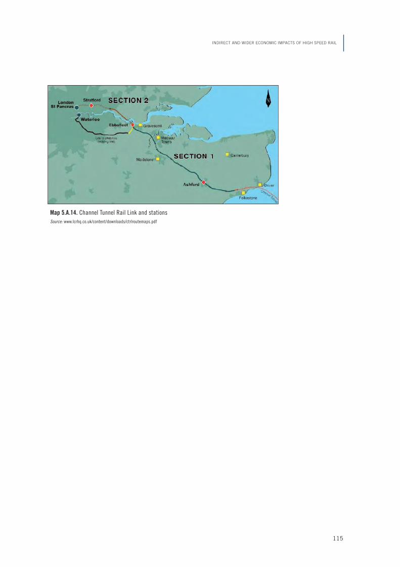
Map 5.A.14. Channel Tunnel Rail Link and stationsSource: www.lcrhq.co.uk/content/downloads/ctrlroutemaps.pdf


115

Map 5.A.15. TGV South and the France-Spain border region


116

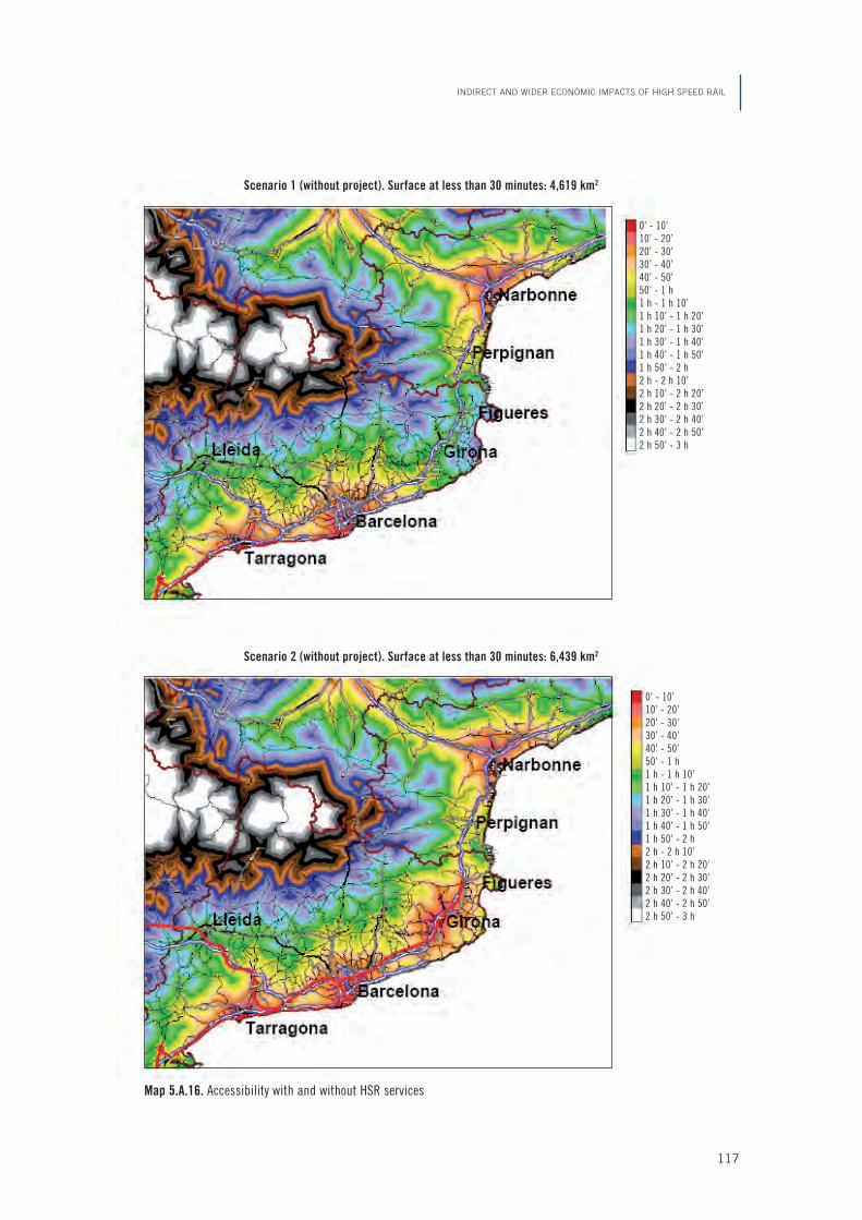
Map 5.A.16. Accessibility with and without HSR services


117

Scenario 1 (without project). Surface at less than 30 minutes: 4,619 km2


Scenario 2 (without project). Surface at less than 30 minutes: 6,439 km2



118

Map 5.A.17. Impacts of changes in accessibility on protected areas

Scenario1 - Scenario 2: Savings of 458 hours/km2 in the interior of protected areas


Investment in high speed rail infrastructure hasdramatically modified the position of the railwaywithin the set of transport alternatives the pas-senger faces in his travel choices. Although thedecline of the market share of railways has notchanged, high speed trains have contributed to asubstantial recovery of rail market share in mediumdistance corridors, where they compete with roadand air transport.

High speed rail generates social benefits, whichcome from time savings, increase in reliability,comfort and safety, and the reduction of conges-tion and accidents in alternative modes. Releas-ing capacity in the conventional network, whichcan be used for freight transport, is an addition-al benefit of the investment in the constructionof new lines.

The key question, central to this research proj -ect, is to determine whether the mentioned so-cial benefits are greater than the costs the socie-ty incurs to carry on the construction andoperation of high speed lines. In other words, thequestion is not whether we like high speed rail ornot, but whether we are willing to pay its costs.

We analyzed under what circumstances the soci-ety may benefit from investing in high speed rail,and when it is worthwhile to delay the invest mentdecision. The high speed rail network can bebuilt gradually, adding new lines once the eco-nomic evaluation of projects offers some guaran-tees for the social profitability of public funds.The economic appraisal of new lines has to lookcarefully to the deviated and generated traffic,the time savings, any additional benefit, and theusers’ willingness to pay.

It is convenient to reinforce the role of the eco-nomic appraisal of the new high speed rail proj-ects, co-financed with European Union funds,instead of using the rhetoric of regional devel-opment to support the expansion of the net-work. High speed rail infrastructure is not goodor bad in global terms. There are socially profit -able projects, and others which are not. Econo-mists can help to identify those projects whichare socially worthy, and whose benefits justifythe sacrifice of leaving other social needs unat-tended. This research project hopes to con-tribute to this aim.

119

Conclusions

ADLER, N., C. NASH, and E. PELS. “Infrastructure Pri-cing: The Case of Airline and High Speed Rail Compe-tition”, Paper presented at the 11th World Conferenceon Transport Research. Berkeley, 2007.

ATKINS. “High-Speed Line Study”. Summary report.London: Department of Environment. Transport and theRegions, 2003.

BARRÓN DE ANGOITI, I. “Construction costs of high spe-ed lines”. UIC. Paris, 2004.

BERNARD, F. “TGV activity”, Paper presented at the UICTraining Seminar, Paris, 2006.

BERRY, S.T. “Estimating discrete-choice models of pro-duct differentiation”. RAND Journal of Economics, 25(1994): 242-262.

BLUM, U., K. E. HAYNES, and C. KARLSSON. “Introduc-tion” to special issue “The regional and urban effectsof high-speed trains”, The Annals of Regional Science,31 (1997): 1-20.

BONNAFOUS A. “The Regional Impact of the TGV”,Transportation 14 (1987): 127-137.

BRÖCKER, J. “Computable general equilibrium analysisin transportation economics”. In HENSHER, D. A., K. J.BUTTON, K. HAYNES and P. STOPHER (eds.). Handbook ofTransport Geography and Spatial Systems: Handbooksin Transport. Vol. 5. Oxford: Elsevier, 2004. Vol 5.

BRÖCKER, J., R. MEYER, N. SCHNEEKLOTH, C. SCHÜR-MANN, K. SPIEKERMANN, and M. WEGENER. “Modellingthe Socio-economic and Spatial Impacts of EUTransport Policy”. IASON (Integrated Appraisal ofSpatial, Economic and Network Effects of TransportInvestments and Policies) Deliverable 6. Funded by5th Framework RTD Programme, Kiel/Dortmund: Ins-titut für Regionalforschung, Christian-Albrechts-

Universität, Kiel/Insti tut für Raumplanung, Universi-tät Dortmund, 2004a.

BRÖCKER, J. et al. “Territorial Impact of EU Transportand TEN Policies”. Final Report of Action 2.1.1. of theEuropean Spatial Planning Observation Network ES-PON 2006. Kiel: Institut für Regionalforschung, Chris-tian-Albrechts-Universität, 2004b.

BURMEISTER, A., and K COLLETIS-WAHL. “TGV et fonc-tions tertiaires: grand vitesse et entreprises de serviceà Lille et Valenciennes”. Transports Urbains, issue 93(October-December, 1996).

CE DELFT. “To shift or not to shift, that’s the question.The environmental performance of the principal modesof freight and passenger transport in the policymakingcontext”. Delft (2003).

CICCONE, A. “Agglomeration effects in Europe”. Euro-pean Economic Review 46, issue 2 (February 2002):213-227.

COST318. “Interaction between High Speed and AirPassenger Transport”. European Commission, Directo-rate General of Transport. Final Report. Luxembourg,1998.

COTO-MILLAN, P., and V. INGLADA. “Social benefit of in-vestment projects: the case for high-speed rail”. Chap-ter 23, Coto-Millán (ed.): Essays on Microeconomicsand Industrial Organisation, Springer (2004).

CRISALLI, R., A. NUZZOLO, A. COMI, and F. SCIANGULA. “ASchedule-Based Mode-Service Choice Model for theAssessment of Competition between Air Transport andHigh speed Services”. Paper presented at the 11th

World Conference on Transport Research, Berkeley,2007.

DE RUS, G. and V. INGLADA. “Análisis coste-beneficio

121

References

del tren de alta velocidad en España”. Economía Apli-cada, 3 (1993): 27-48.

—. “Cost-benefit analysis of the high-speed train inSpain”. The Annals of Regional Science, 31 (1997):175-188.

DE RUS, G., and C. A. NASH. “In what circumstances isinvestment in HSR worthwhile?”. Working paper. 4thAnnual Conference on “Railroad Industry Structure,Competition and Investment”. Madrid: UniversidadCarlos III, 2007.

DE RUS, G., and G. NOMBELA. “Is the investment in highspeed rail socially profitable?”. Journal of TransportEconomics and Policy (2007).

DE RUS, G., and C. ROMÁN. “Economic Evaluation of theHigh Speed Rail Madrid-Barcelona”. 8th Nectar Confe-rence. Las Palmas (2005).

—. “Análisis Económico de la Línea de Alta VelocidadMadrid-Barcelona”. Revista de Economía Aplicada XIV,42 (2006): 35-80.

DE RUS, G., J. CAMPOS, and G. NOMBELA. Economía delTransporte. Barcelona: Antoni Bosch, 2003.

DEPARTMENT FOR TRANSPORT. “Transport, Wider EconomicBenefits, and Impacts on GDP”. Technical Paper (2005).Available online at: http://www.dft.gov.uk/pgr/ econo-mics/rdg/webia/transportwidereconomicbenefi3137

DEPARTMENT OF ENVIRONMENT, TRANSPORT AND THE RE-GIONS. The incidence of imperfect competition in UKsectors and regions. London, 1999.

—. High speed line study. Feasibility study by Atkinsfor the Strategic Rail Authority. London, 2004.

DORNBUSCH, J. “Nantes, sept ans après l’arrivée du TGVAtlantique”. Notes de Synthese du SES, Mai-Juin(1997).

ELHORST, J. P., J. OOSTERHAVEN, and A. E. ROMP. “Inte-gral Cost-Benefit Analysis of Maglev Technology UnderMarket Imperfections”. SOM Research Report, Univer-sity of Groningen, (2004). Available online at http://irs.ub.rug.nl/ppn/268887764

EUROPEAN COMMISSION. Council Directive 96/48/EC onthe interoperability of the trans-European high speedrail system. Brussels (1996).

—. “Guide to cost-benefit analysis of major projects. Inthe context of EC regional policy”. Directorate-GeneralXVI. Brussels (1997).

—. “European transport policy for 2010: time to deci-de”. White Paper, Brussels (2001).

—. “High Level Group on the Trans-European TransportNetwork”. Report. Brussels: European Commission,2003.

—. “Trans-European Transport Network, TEN-T PriorityAxes and Projects”. Brussels: European Commission,2005.

EVANS, AW. “Accidental fatalities in transport”. JRSSSeries A, 162 (2) (2003): 253-260.

FLYVBJERG, B., M. K. SKAMRIS, and S. L. BUHL. “Whatcauses cost overrun in transport infrastructure projects?”.Transport Reviews, 24 (1) (2004): 3-18.

FRIEBEL, G., and M. NIFFKA. “The Functioning of Inter-modal Competition in the Transportation Market: Evi-dence from the Entry of Low-cost Airlines in Germany”(2005). Available online at SSRN: http://ssrn.com/abs-tract=745164

FUJITA, M., and J. THISSE. The Economics of Agglome-ration. Cambridge: Cambridge University Press, 2002.

FUJITA, M., P. KRUGMAN, and A. J. VENABLES. The spatialeconomy: cities, regions and international trade. Cam-bridge MA: MIT Press, 1999.

GALLOIS, L. “Achievements and Outlooks for the Deve-lopment of High Speed Rail in Europe”, Paper presen-ted at EurailSpeed, Milan (2005).

GIBSON, S., G. COOPER, and B. BELL. “Capacity chargeson the UK rail network”. Journal of Transport Econo-mics and Policy, 36 (2) (2002): 341-354.

GIVONI, M. “Aircraft and High Speed Train Substitution:the Case for Airline and Railway Integration”. Unpu-blished PhD thesis. London: University College, 2005.

GIVONI, M., and D. BANISTER. “Airline and Railway Inte-gration”, Transport Policy, 13 (2006): 386-397.

GÓMEZ-IBAÑEZ, J. A., and G. DE RUS. “Competition in theRailway Industry: An International Comparative Analy-sis”. Edward Elgar (2006).

GONZÁLEZ-SAVIGNAT, M. “Will the High speed Train Com-


122

pete Against the Private Vehicle?”. Transport Reviews,24, 3 (2004): 293-316.

GOODWIN P. B. “A Review of New Demand Elasticitieswith Special Reference to Short and Long Run Effectsof Price Changes”. Journal of Transport Economics andPolicy, 26(2) (1992): 155-169.

GRAHAM, D. “Wider economic benefits of transport im-provements: link between agglomeration and producti-vity”. Stage 1 Report. Imperial College. London: De-partment for Transport, 2005. Available online at:http://www.dft.gov.uk/pgr/economics/rdg/webia/widere-conomicbenefitsoftrans3138

GRIMME, W. “Air/Rail Intermodality – Recent Experien-ces from Germany”. Aerlines Magazine, 34 (2006).

GUNN, H. “SCGE Models: Relevance and Accessibilityfor Use in the UK, with emphasis on Implications forEvaluation of Transport Investments”. Final Report toDepartment of Transport. London: Cambridge RANDEurope, 2004.

GUTIÉRREZ, J. “Location, economic potential and dailyaccessibility: an analysis of the accessibility impact ofthe high-speed line Madrid–Barcelona–French border”.Journal of Transport Geography 9, issue 4 (2001):229-242

GUTIÉRREZ, J., R. GONZÁLEZ, and G. GÓMEZ. “The Euro-pean high-speed train network: predicted effects on ac-cessibility patterns”. Journal of Transport Geography4, issue 4 (December 1996): 227-238

HARBERGER, A. C. Project evaluation: collected papers.The University of Chicago Press (1972).

HAYNES, K. E. “Labour markets and regional transpor-tation improvements: the case of high-speed trains: Anintroduction and review”. The Annals of RegionalScience, 31 (1997): 57-76.

HENSHER, D. A. Value of Business Travel Time. Oxford:Pergamon Press, 1977.

HOOD, C. P. Shinkansen: from bullet train to symbol ofmodern Japan. Routledge (2006).

INFRAS/IWW. “External costs of transport”. Reportcommissioned by UIC. Zurich-Karlsruhe-Paris (2000).

INSTITUTE FOR TRANSPORT STUDIES, UNIVERSITY OF LEEDS.Values of Travel Time Saving in the UK. Leeds, UK:Institute for Transport Studies, 2003.

IVALDI, M., and C. VIBES. Price Competition in the In-tercity Passenger Transport Market: A Simulation Mo-del. Toulouse School of Economics. Mimeo (2005).

JANIC, M. “A Model of Competition between High Spe-ed Rail and Air Transport”, Transportation Planningand Technology, 17, 1 (1993): 1-23.

—. “High Speed Rail and Air Passenger Transport”.Proc. Instn Mech. Engrs., 21, Part F (2003): 259-269.

JARA DÍAZ, S. “On the relation between users’ benefitsand the economic effects of transportation activities”.Journal of Regional Science, 26 (1986): 379-391.

KLEIN, O., and G. CLAISSE. Le TGV-Atlantique: entre re-cession et concurrence. Lyon: LET, 1997.

KUMBHAKAR, S. C., and C. A .K. LOVELL. StochasticFrontier Analysis. Cambridge: University Press, 2000.

LAFFONT, J. J., and J. TIROLE. A Theory of Incentives inProcurement and Regulation. Cambridge: MIT Press,1993.

LAIRD, J. J., J. NELLTHORP, and P. J. MACKIE. “Networkeffects and total economic impact in transport apprai-sal”. Transport Policy 12, issue 6 (November 2005):537-544.

LEBOEUF, M. “Traffic Forecasts for High speed TrainServices”. Paper presented at the UIC Training Semi-nar, Paris (2006).

LEVINSON, D., J. M. MATHIEU, D. GILLEN, and A. KANAFA-NI. “The full cost of high speed rail: an engineering ap-proach”. The Annals of Regional Science 31 (1997):189-215.

LÓPEZ-PITA, A. Railway and Plane in the EuropeanTransport System. CENIT Ediciones UPC (2001a).

—. “A new challenge for Europe’s railways: Internatio-nal passenger services”. Rail International (2001b):10-16.

LÓPEZ-PITA, A., and F. ROBUSTÉ. “Introduction to an Eva-luation of the Impact of High Speed Rail Infrastructu-re in Europe”. Paper presented at TRB 2003 AnnualMeeting (2003).

—. “Impact of High speed Lines in Relation to VeryHigh Frequency Air Services”. Journal of Public Trans-portation 8, 2 (2005): 17-36.

REFERENCES

123

LÓPEZ-PITA, A., F. ROBUSTÉ, P. F. TEIXEIRA, A. BACHILLER,and C. CASAS. “Impacto Comercial en la Aviación de laExplotación de Líneas de Alta Velocidad en Europa:1981-2006”. CENIT, UPC: Mimeo, 2006.

MARKS, P., A. S. FOWKES, and C. A. NASH. “Valuing LongDistance Business Travel Time Savings for Evaluation:A Methodological Review and Application”, PTRCSummer Annual Meeting (1986).

MARTIN, F. “Justifying a high-speed rail project: socialvalue vs. regional growth”. The Annals of RegionalScience, 31 (1997): 155-174.

MARTÍN, J. C., and G. NOMBELA. “Microeconomic Im-pacts of Investment in High Speed Rail in Spain”. TheAnnals of Regional Science. Forthcoming (2007).

MATHIS, P. et al. “Transport services and networks: te-rritorial trends and basic supply of infrastructure for te-rritorial cohesion”. Final Report of Action 1.2.1 of theEuropean Spatial Planning Observation Network 2006(ESPON) (2004).

MCFADDEN, D. T. Travel Demand: a Behavioural Analy-sis. Amsterdam: North-Holland, 1975.

MOHRING, H. Transportation economics. Ballinger Pu-blishing Company (1976).

NASH, C. A. “The Case for High Speed Rail”. Investiga-ciones Económicas, 15(2) (1991): 337-354.

NELLTHORP, J., T. SANSOM, P. BICKEL, C. DOLL, and G.LINDBERG. “Valuation conventions for UNITE”. UNITE(UNIfication of accounts and marginal costs for Trans-port Efficiency), 5th Framework RTD Programme. ITS,Leeds: University of Leeds, 2001.

OOSTERHAVEN, J., and J. P. ELHORST. “Indirect economicbenefits of transport infrastructure investments”. EnDULLAERT, W., B. JOURQUIN, and J. B. POLAK (ed.).Across the Border: Building on a Quarter Century ofTransport Research in the Benelux. Antwerp: De Bo-eckn, 2003.

OUM, T. H., W. G. WATERS, and J. S. YONG. “Concepts ofPrice Elasticities of Transport Demand and Recent Em-pirical Estimates: an Interpretative Survey”. Journal ofTransport Economics and Policy, 26 (2) (1992): 139-169.

PARK, Y., and H-K. HA. “Analysis of the Impact of Highspeed Railroad Service on Air Transport Demand”.Transportation Research, Part E, 42 (2006): 95-104.

PAVAUX, J. “Rail/air Complementarity in Europe: Theimpact of High speed Train Services”. Institute of AirTransport, Paris. ISBN 2-908537-04-4, 1991.

PLASSARD, F., and O. COINTET-PINELL. “Les effets socio-économique du TGV en Bourgogne et Rhônes Alpes”.DATAR, INRETS, OEST, SNCF, 1986.

—. “High speed transport and regional development”.In Regional policy, transport network. Paris: EuropeanConference of Ministers of Transport, 1994.

PRESTON, J., and G. WALL. “The Impact of High SpeedTrains on Socio-economic Activity”. Paper presented atthe 11th WCTRS, Berkeley, 2007.

QUINET, E., and R. VICKERMANN. “Principles of TransportEconomics”. Edward Elgar, Cheltenham-Northampton,2004.

SACTRA (Standing Advisory Committee on Trunk RoadAssessment). Transport and the Economy. London:Stationery Office, 1999.

SDG. “High Speed Rail: International Comparisons”.Prepared by Steer Davies Gleave for the Commissionfor Integrated Transport. London, 2004.

SELLNICK, O. “High speed Traffic of Deutsche BahnAG”. Paper presented at the UIC Training Seminar. Pa-ris, 2006.

SES. “Evaluation de l’impact du TGV Nord-Européensur la mobilité”. Les Etudes du SES, 1998.

SPIEKERMANN, K., and M. WEGENER. “The shrinking con-tinent: new time-space maps of Europe”. Environmentand Planning B 21, issue 6 (1994): 653-73.

TRANSPORT AND MOBILITY LEUVEN. ASSESS Final Report,Annex 21 (2005).

TURRÓ, M. Going Transeuropean: planning and finan-cing transport networks for Europe. Oxford: Elsevier,2000.

UIC. “Study on the Influence of Low-cost Air Compa-nies and Long Distance Coaches on the Demand ofPassengers Rail Services in Europe”. Paris: Internatio-nal Union of Railways, 2003

—. “High Speed. Rail’s leading asset for customersand society”. UIC Publications, Paris (2005a). Availa-ble online at www.uic.asso.fr


124

—. “Estimation des resources et des activités écono-miques liées a la grande vitesse”. Prepared by CENIT(Center for Innovation in Transport, Universitat Politec-nica de Catalunya), Paris, 2005b.

—. “Railway time-series data 1970-2004”. Paris: UICPublications, 2006.

ULIED, A. “Union’s Territorial Strategies Linked toTENs”. DGTREN. European Commission, 1997.

VENABLES, A. “Evaluating urban transport improve-ments: cost-benefit analysis in the presence of agglo-meration and income taxation”. London School of Eco-nomics: Mimeo, 2004.

VENABLES, A., and M. GASIOREK. “The Welfare Implica-tions of Transport Improvements in the Presence ofMarket Failure Part 1”. Report to Standing AdvisoryCommittee on Trunk Road Assessment. London: DETR(Department of the Environment, Transport and the Re-gions), 1999.

VICKERMAN, R. “The regional impacts of Trans-Europeannetworks”. The Annals of Regional Science 29 (1995):237-254.

—. “High-speed rail in Europe: experience and issuesfor future development”. The Annals of RegionalScience 31 (1997): 21-38.

—. “Trans-European Networks: policy and appraisal”.Scienze Regionale- Italian Journal of Regional Science5, issue 2 (2006): 71-87.

—. “Cost-benefit analysis and large-scale infrastructu-re projects: state of the art and challenges”. Environ-ment and Planning B 34, issue 4 (2007): 598-610.

VICKERMAN, R., K. SPIEKERMANN, and M. WEGENER. “Ac-cessibility and regional development in Europe”. Re-gional Studies 33, issue 1 (1999): 1-15.

WARDMAN, M. “A review of British evidence on Time andService Quality”. Transportation Research E 2(3),(2001): 107-128.

WEGENER, M., and D. BÖKEMANN. “The SASI Model: Mo-del Structure”. SASI Deliverable D8. Berichte aus demInstitut für Raumplanung 40. Dortmund: Institut fürRaumplanung, Universität Dortmund, 1998. Availableonline at: http://irpud.raumplanung.uni-dortmund.de/irpud/pro /sasi/ber40.pdf

WEI, W., and M. HANSEN. “Impact of Aircraft Size andSeat Availability on Airlines’ Demand and Market Sha-re in Duopoly Markets”. Transportation Research E 41(2005): 315-327.

WHITELEGG, J. “Transport for a sustainable future: Thecase for Europe”. London: Belhaven Press, 1993.

WILKEN, D. “Area and Limits of Competition betweenHigh Speed Rail and Air”. Dresden: Proc. Think-UpProject Workshop, 2000.

YAO, E., and T. MORIKAWA. “A study on integrated inter-city travel demand model”. Paper presented at the10th International Conference on Travel Behaviour Re-search. Lucerne, 2003.

REFERENCES

125

Graph 1.1: HSR models according to the relationship with conventional services .......................... 21

Graph 1.2: Time slots in railways and the provision of HSR services ............................................. 22

Graph 1.3: Average cost per kilometer of new HSR infrastructure ................................................. 25

Graph 1.4: Evolution of accumulated traffic: Asia vs. Europe ....................................................... 31

Graph 2.1: Project timeline: construction and operation period .................................................... 35

Graph 2.2: One-way traffic projections (under faster growth assumption) ...................................... 38

Graph 2.3: Number of trains needed under alternative capacity assumptions ............................... 40

Graph 2.4: Number of trains needed under alternative speed assumptions ................................... 41

Graph 2.5: Number of trains needed under alternative initial annual demand assumptions ........... 41

Graph 2.6: Acquisition costs per year under alternative scenarios (in € million) ........................... 44

Graph 2.7: Acquisition costs per year under alternative train capacities (in € million) .................. 45

Graph 2.8: Operation costs per year under alternative scenarios (in € million) ............................. 46

Graph 2.9: Operation costs per year under alternative train capacities (in € million) .................... 46

Graph 2.10: Maintenance costs per year under alternative train capacities (in € million) ................ 47

Graph 2.11a: NPV cost distribution depending on initial demand .................................................... 48

Graph 2.11b: NPV cost distribution depending on commercial speed ............................................... 49

Graph 2.11c: NPV cost distribution depending on train capacity ..................................................... 49

Graph 2.11d: NPV cost distribution depending on line length .......................................................... 50

Graph 3.1: Rail passenger and freight volumes (1979 to 2004/05) .............................................. 55

Graph 3.2a: First year demand required for NPV = 0 (α = 0.2 θ = 3%) ......................................... 66

Graph 3.2b: First year demand required for NPV = 0 (α = 0.2 θ = 4%) ......................................... 67

Graph 3.2c: First year demand required for NPV = 0 (α = 0.4 θ = 3%) ......................................... 67

127

List of Graphs

Graph 3.2d: First year demand required for NPV = 0 (α = 0.4 θ = 4%) ......................................... 68

Graph 4.1: The modal competitive advantage of HSR .................................................................. 73

Graph 4.2: The traveller’s decision among alternative transport modes ......................................... 77


128

Map 5.A.1: Rail network development to 2021 ............................................................................. 104

Map 5.A.2: Rail investment (million €) to 2015 ........................................................................... 105

Map 5.A.3: Rail investment (million €) to 2030 ........................................................................... 106

Map 5.A.4: Potential accessibility by rail, 2001 ........................................................................... 107

Map 5.A.5: Multimodal accessibility (road/rail/air), 2001 .............................................................. 108

Map 5.A.6: Connectivity to rail stations ........................................................................................ 109

Map 5.A.7: Change in accessibility 2001-2021: all TEN/TINA projects completed ......................... 110

Map 5.A.8: Change in GDP per capita to 2021 due to changes in accessibility in Map 5.A.7 (using SASI model) .............................................................................................................. 111

Map 5.A.9: Change in welfare as % GDP per capita to 2021 due to changes in accessibility in Map 5.A.7 (using CGEurope model) ............................................................................ 112

Map 5.A.10: Accessibility to rail, Spain, 2005 ............................................................................... 113

Map 5.A.11: Rail services, Spain, 2006 ......................................................................................... 113

Map 5.A.12: HSR services, Spain, 2006 ........................................................................................ 114

Map 5.A.13: North-west European HSR Network ............................................................................. 114

Map 5.A.14: Channel Tunnel Rail Link and stations ........................................................................ 115

Map 5.A.15: TGV South and the France-Spain border region ........................................................... 116

Map 5.A.16: Accessibility with and without HSR services ................................................................ 117

Map 5.A.17: Impacts of changes in accessibility on protected areas ................................................ 118

129

List of Maps

Table 1.1: Cost of HRS infrastructures maintenance by country ....................................................... 26

Table 1.2: HRS technology in Europe: types of train ........................................................................ 27

Table 1.3: Comparison of operating and maintenance cost by HRS technology (euros) ...................... 28

Table 1.4: External costs of car, rail and air (euros/1,000 passenger-km) ......................................... 30

Table 1.5: Evolution of high speed rail traffic in Europe (1994–2004) ............................................. 31

Table 2.1: Traffic projections with alternative initial demand assumptions ........................................ 37

Table 2.2: The reference case: main parameter values ..................................................................... 42

Table 2.3: Infrastructure costs per year (reference case) .................................................................. 43

Table 2.4: Annual infrastructure costs under different line lengths (euros) ...................................... 43

Table 2.5: Total costs (at t=0) of a HSR line under alternative assumptions (euros) .......................... 48

Table 3.1: Energy consumption (MJ/Seat Km) ................................................................................. 52

Table 3.2: Value of time savings for rail passengers in the UK ......................................................... 53

Table 3.3: External costs (euros/1,000 pass-km) ............................................................................. 54

Table 3.4: Appraisal of options 1 and 8 (£bn, present value) ........................................................... 56

Table 3.5: Cost benefit analysis results, option 1 (% of Total Benefits or Costs) ............................... 57

Table 3.6: Benefits of Madrid-Seville high speed train (millions of 1987 pesetas) ............................ 59

Table 3.7: Estimated costs of a 500-km HSR line in Europe (2004) ................................................ 65

Table 3.8: First year demand thresholds for NPV=0 (r=5% T=40 Ct=32.5 Cq=91.5 Cc=62) ............... 68

Table 3.9: First year demand thresholds for NPV=0 (r=3% T=40 Ct=32.5 Cq=91.5 Cc=62) ............... 69

Table 4.1: Travel time and rail market share on selected corridors .................................................... 74

Table 4.2: Modal market share before and after HSR (selected routes) ............................................. 75

Table 4.3: Airfares vs. HSR fares on selected European corridors ..................................................... 76

131

List of Tables

Table 4.4: Intermodal competition effects: own-price elasticities, marginal costs, and pricemargin simulations ......................................................................................................... 86

Table 4.5: Simulation: cross-price elasticities (α = 0.04) ................................................................ 87

Table 5.1: HSR projects in priority TENs ......................................................................................... 92


132

Economía y SociedadInformes 2009

Economía y Sociedad

Economic Analysis of H

igh Speed Rail in EuropeInform

es 2009

Ginés de Rus (Ed.)

Ignacio BarrónJavier Campos

Philippe GagnepainChris Nash

Andreu UliedRoger Vickerman

Plaza de San Nicolás, 448005 BilbaoEspañaTel.: + 34 94 487 52 52Fax: + 34 94 424 46 21

Paseo de Recoletos, 1028001 MadridEspañaTel.: +34 91 374 54 00Fax: +34 91 374 85 22

[email protected]

Economic Analysisof High Speed Railin Europe

economic analysis of high speed rail in europe · 2017. 6. 21. · economía y sociedad informes...

Documents