ergebnissedermathematik volume51 … the aim of this monograph is to give an overview of various...
TRANSCRIPT
Ergebnisse der Mathematik Volume 51und ihrer Grenzgebiete
3. Folge
A Series of Modern Surveysin Mathematics
Editorial Board
M. Gromov, Bures-sur-Yvette J. Jost, LeipzigJ. Kollár, Princeton G. Laumon, OrsayH. W. Lenstra, Jr., Leiden J. Tits, ParisD. B. Zagier, Bonn G. Ziegler, Berlin
Managing Editor R. Remmert, Münster

Boris Khesin • Robert Wendt
The Geometry ofInfinite-DimensionalGroups
123
Boris KhesinRobert WendtDepartment of MathematicsUniversity of Toronto40 St. George StreetToronto, ONCanada M5S 2E4e-mail: [email protected] and
ISBN 978-3-540-77262-0 e-ISBN 978-3-540-77263-7
DOI 10.1007/978-3-540-77263-7
Ergebnisse der Mathematik und ihrer Grenzgebiete. 3. Folge / A Series of ModernSurveys in Mathematics ISSN 0071-1136
Library of Congress Control Number: 2008932850
Mathematics Subject Classification (2000): 22E65, 37K05, 58B25, 53D30
© 2009 Springer-Verlag Berlin Heidelberg
This work is subject to copyright. All rights are reserved, whether the whole or part of the material isconcerned, specifically the rights of translation, reprinting, reuse of illustrations, recitation, broadcasting,reproduction on microfilm or in any other way, and storage in data banks. Duplication of this publicationor parts thereof is permitted only under the provisions of the German Copyright Law of September 9,1965, in its current version, and permission for use must always be obtained from Springer. Violations areliable to prosecution under the German Copyright Law.
The use of general descriptive names, registered names, trademarks, etc. in this publication does not imply,even in the absence of a specific statement, that such names are exempt from the relevant protective lawsand regulations and therefore free for general use.
Typesetting: by the author using a Springer TEX macro packageProduction: LE-TEX Jelonek, Schmidt & Vöckler GbR, LeipzigCover design: WMX Design GmbH, Heidelberg
Printed on acid-free paper
9 8 7 6 5 4 3 2 1
springer.com

To our Teachers:
to Vladimir Igorevich Arnold
and to the memory of Peter Slodowy


Preface
The aim of this monograph is to give an overview of various classes of infinite-dimensional Lie groups and their applications, mostly in Hamiltonian me-chanics, fluid dynamics, integrable systems, and complex geometry. We havechosen to present the unifying ideas of the theory by concentrating on specifictypes and examples of infinite-dimensional Lie groups. Of course, the selectionof the topics is largely influenced by the taste of the authors, but we hopethat this selection is wide enough to describe various phenomena arising in thegeometry of infinite-dimensional Lie groups and to convince the reader thatthey are appealing objects to study from both purely mathematical and moreapplied points of view. This book can be thought of as complementary to theexisting more algebraic treatments, in particular, those covering the struc-ture and representation theory of infinite-dimensional Lie algebras, as well asto more analytic ones developing calculus on infinite-dimensional manifolds.
This monograph originated from advanced graduate courses and mini-courses on infinite-dimensional groups and gauge theory given by the firstauthor at the University of Toronto, at the CIRM in Marseille, and at theEcole Polytechnique in Paris in 2001–2004. It is based on various classical andrecent results that have shaped this newly emerged part of infinite-dimensionalgeometry and group theory.
Our intention was to make the book concise, relatively self-contained, anduseful in a graduate course. For this reason, throughout the text, we haveincluded a large number of problems, ranging from simple exercises to openquestions. At the end of each section we provide bibliographical notes, tryingto make the literature guide more comprehensive, in an attempt to bring theinterested reader in contact with some of the most recent developments inthis exciting subject, the geometry of infinite-dimensional groups. We hopethat this book will be useful to both students and researchers in Lie theory,geometry, and Hamiltonian systems.
It is our pleasure to thank all those who helped us with the preparation ofthis manuscript. We are deeply indebted to our teachers, collaborators, and
VIII Preface
friends, who influenced our view of the subject: V. Arnold, Ya. Brenier,H. Bursztyn, Ya. Eliashberg, P. Etingof, V. Fock, I. Frenkel, D. Fuchs,A. Kirillov, F.Malikov, G. Misiolek, R. Moraru, N. Nekrasov, V. Ovsienko,C. Roger, A. Rosly, V. Rubtsov, A. Schwarz, G. Segal, M. Semenov-Tian-Shansky, A. Shnirelman, P. Slodowy, S. Tabachnikov, A. Todorov,A. Veselov, F.Wagemann, J. Weitsman, I. Zakharevich, and many others.We are particularly grateful to Alexei Rosly, the joint projects with whominspired a large part, in particular the “application chapter,” of this book,and who made numerous invaluable remarks on the manuscript. We thankthe participants of the graduate courses for their stimulating questions andremarks. Our special thanks go to M.Peters and the Springer team for theirinvariable help and to D.Kramer for careful editing of the text.
We also acknowledge the support of the Max-Planck Institute in Bonn, theInstitut des Hautes Etudes Scientifiques in Bures-sur-Yvette, the Clay Math-ematics Institute, as well as the NSERC research grants. The work on thisbook was partially conducted during the period the first author was employedby the Clay Mathematics Institute as a Clay Book Fellow.
Finally, we thank our families (kids included!) for their tireless moralsupport and encouragement throughout the over-stretched work on themanuscript.
Contents
Preface . . . . . . . . . . . . . . . . . . . . . . . . . . . . . . . . . . . . . . . . . . . . . . . . . . . . . . . . VII
Introduction . . . . . . . . . . . . . . . . . . . . . . . . . . . . . . . . . . . . . . . . . . . . . . . . . . . 1
I Preliminaries . . . . . . . . . . . . . . . . . . . . . . . . . . . . . . . . . . . . . . . . . . . . . . 71 Lie Groups and Lie Algebras . . . . . . . . . . . . . . . . . . . . . . . . . . . . . . 7
1.1 Lie Groups and an Infinite-Dimensional Setting . . . . . . . 71.2 The Lie Algebra of a Lie Group . . . . . . . . . . . . . . . . . . . . . 91.3 The Exponential Map . . . . . . . . . . . . . . . . . . . . . . . . . . . . . . 121.4 Abstract Lie Algebras . . . . . . . . . . . . . . . . . . . . . . . . . . . . . . 15
2 Adjoint and Coadjoint Orbits . . . . . . . . . . . . . . . . . . . . . . . . . . . . . 172.1 The Adjoint Representation . . . . . . . . . . . . . . . . . . . . . . . . 172.2 The Coadjoint Representation . . . . . . . . . . . . . . . . . . . . . . 19
3 Central Extensions . . . . . . . . . . . . . . . . . . . . . . . . . . . . . . . . . . . . . . 213.1 Lie Algebra Central Extensions . . . . . . . . . . . . . . . . . . . . . 223.2 Central Extensions of Lie Groups . . . . . . . . . . . . . . . . . . . . 24
4 The Euler Equations for Lie Groups . . . . . . . . . . . . . . . . . . . . . . . 264.1 Poisson Structures on Manifolds . . . . . . . . . . . . . . . . . . . . . 264.2 Hamiltonian Equations on the Dual of a Lie Algebra . . . 294.3 A Riemannian Approach to the Euler Equations . . . . . . 304.4 Poisson Pairs and Bi-Hamiltonian Structures . . . . . . . . . . 354.5 Integrable Systems and the Liouville–Arnold Theorem . 38
5 Symplectic Reduction . . . . . . . . . . . . . . . . . . . . . . . . . . . . . . . . . . . . 405.1 Hamiltonian Group Actions . . . . . . . . . . . . . . . . . . . . . . . . . 415.2 Symplectic Quotients . . . . . . . . . . . . . . . . . . . . . . . . . . . . . . 42
6 Bibliographical Notes . . . . . . . . . . . . . . . . . . . . . . . . . . . . . . . . . . . . 44
II Infinite-Dimensional Lie Groups: Their Geometry, Orbits,and Dynamical Systems . . . . . . . . . . . . . . . . . . . . . . . . . . . . . . . . . . . 471 Loop Groups and Affine Lie Algebras . . . . . . . . . . . . . . . . . . . . . . 47
1.1 The Central Extension of the Loop Lie algebra . . . . . . . . 47

X Contents
1.2 Coadjoint Orbits of Affine Lie Groups . . . . . . . . . . . . . . . . 521.3 Construction of the Central Extension of the Loop
Group . . . . . . . . . . . . . . . . . . . . . . . . . . . . . . . . . . . . . . . . . . . 581.4 Bibliographical Notes . . . . . . . . . . . . . . . . . . . . . . . . . . . . . . 65
2 Diffeomorphisms of the Circle and the Virasoro–Bott Group . . 672.1 Central Extensions . . . . . . . . . . . . . . . . . . . . . . . . . . . . . . . . 672.2 Coadjoint Orbits of the Group of Circle Diffeomorphisms 702.3 The Virasoro Coadjoint Action and Hill’s Operators . . . 722.4 The Virasoro–Bott Group and the Korteweg–de Vries
Equation . . . . . . . . . . . . . . . . . . . . . . . . . . . . . . . . . . . . . . . . . 802.5 The Bi-Hamiltonian Structure of the KdV Equation . . . 822.6 Bibliographical Notes . . . . . . . . . . . . . . . . . . . . . . . . . . . . . . 86
3 Groups of Diffeomorphisms . . . . . . . . . . . . . . . . . . . . . . . . . . . . . . . 883.1 The Group of Volume-Preserving Diffeomorphisms
and Its Coadjoint Representation . . . . . . . . . . . . . . . . . . . . 883.2 The Euler Equation of an Ideal Incompressible Fluid . . . 903.3 The Hamiltonian Structure and First Integrals
of the Euler Equations for an Incompressible Fluid . . . . 913.4 Semidirect Products: The Group Setting for an Ideal
Magnetohydrodynamics and Compressible Fluids . . . . . . 953.5 Symplectic Structure on the Space of Knots
and the Landau–Lifschitz Equation . . . . . . . . . . . . . . . . . . 993.6 Diffeomorphism Groups as Metric Spaces . . . . . . . . . . . . . 1053.7 Bibliographical Notes . . . . . . . . . . . . . . . . . . . . . . . . . . . . . . 109
4 The Group of Pseudodifferential Symbols . . . . . . . . . . . . . . . . . . . 1114.1 The Lie Algebra of Pseudodifferential Symbols . . . . . . . . 1114.2 Outer Derivations and Central Extensions of ψDS . . . . . 1134.3 The Manin Triple of Pseudodifferential Symbols . . . . . . . 1174.4 The Lie Group of α-Pseudodifferential Symbols . . . . . . . 1194.5 The Exponential Map for Pseudodifferential Symbols . . 1224.6 Poisson Structures on the Group
of α-Pseudodifferential Symbols . . . . . . . . . . . . . . . . . . . . . 1244.7 Integrable Hierarchies on the Poisson Lie Group ˜GINT . 1294.8 Bibliographical Notes . . . . . . . . . . . . . . . . . . . . . . . . . . . . . . 132
5 Double Loop and Elliptic Lie Groups . . . . . . . . . . . . . . . . . . . . . . 1345.1 Central Extensions of Double Loop Groups
and Their Lie Algebras . . . . . . . . . . . . . . . . . . . . . . . . . . . . . 1345.2 Coadjoint Orbits . . . . . . . . . . . . . . . . . . . . . . . . . . . . . . . . . . 1365.3 Holomorphic Loop Groups and Monodromy . . . . . . . . . . 1385.4 Digression: Definition of the Calogero–Moser Systems . . 1425.5 The Trigonometric Calogero–Moser System
and Affine Lie Algebras . . . . . . . . . . . . . . . . . . . . . . . . . . . . 1465.6 The Elliptic Calogero–Moser System and Elliptic Lie
Algebras . . . . . . . . . . . . . . . . . . . . . . . . . . . . . . . . . . . . . . . . . 1495.7 Bibliographical Notes . . . . . . . . . . . . . . . . . . . . . . . . . . . . . . 152

Contents XI
III Applications of Groups: Topologicaland Holomorphic Gauge Theories . . . . . . . . . . . . . . . . . . . . . . . . . . 1551 Holomorphic Bundles and Hitchin Systems . . . . . . . . . . . . . . . . . 155
1.1 Basics on Holomorphic Bundles . . . . . . . . . . . . . . . . . . . . . 1551.2 Hitchin Systems . . . . . . . . . . . . . . . . . . . . . . . . . . . . . . . . . . . 1591.3 Bibliographical Notes . . . . . . . . . . . . . . . . . . . . . . . . . . . . . . 162
2 Poisson Structures on Moduli Spaces . . . . . . . . . . . . . . . . . . . . . . . 1632.1 Moduli Spaces of Flat Connections on Riemann
Surfaces . . . . . . . . . . . . . . . . . . . . . . . . . . . . . . . . . . . . . . . . . . 1632.2 Poincare Residue and the Cauchy–Stokes Formula . . . . . 1702.3 Moduli Spaces of Holomorphic Bundles . . . . . . . . . . . . . . 1732.4 Bibliographical Notes . . . . . . . . . . . . . . . . . . . . . . . . . . . . . . 179
3 Around the Chern–Simons Functional . . . . . . . . . . . . . . . . . . . . . . 1803.1 A Reminder on the Lagrangian Formalism . . . . . . . . . . . . 1803.2 The Topological Chern–Simons Action Functional . . . . . 1843.3 The Holomorphic Chern–Simons Action Functional . . . . 1873.4 A Reminder on Linking Numbers . . . . . . . . . . . . . . . . . . . . 1893.5 The Abelian Chern–Simons Path Integral and Linking
Numbers . . . . . . . . . . . . . . . . . . . . . . . . . . . . . . . . . . . . . . . . . 1923.6 Bibliographical Notes . . . . . . . . . . . . . . . . . . . . . . . . . . . . . . 196
4 Polar Homology . . . . . . . . . . . . . . . . . . . . . . . . . . . . . . . . . . . . . . . . . 1974.1 Introduction to Polar Homology . . . . . . . . . . . . . . . . . . . . . 1974.2 Polar Homology of Projective Varieties . . . . . . . . . . . . . . . 2024.3 Polar Intersections and Linkings . . . . . . . . . . . . . . . . . . . . . 2064.4 Polar Homology for Affine Curves . . . . . . . . . . . . . . . . . . . 2094.5 Bibliographical Notes . . . . . . . . . . . . . . . . . . . . . . . . . . . . . . 211
Appendices . . . . . . . . . . . . . . . . . . . . . . . . . . . . . . . . . . . . . . . . . . . . . . . . . . . . 213A.1 Root Systems . . . . . . . . . . . . . . . . . . . . . . . . . . . . . . . . . . . . . . . . . . . 213
1.1 Finite Root Systems . . . . . . . . . . . . . . . . . . . . . . . . . . . . . . . 2131.2 Semisimple Complex Lie Algebras . . . . . . . . . . . . . . . . . . . 2151.3 Affine and Elliptic Root Systems . . . . . . . . . . . . . . . . . . . . 2161.4 Root Systems and Calogero–Moser Hamiltonians . . . . . . 218
A.2 Compact Lie Groups . . . . . . . . . . . . . . . . . . . . . . . . . . . . . . . . . . . . . 2212.1 The Structure of Compact Groups . . . . . . . . . . . . . . . . . . . 2212.2 A Cohomology Generator for a Simple Compact Group 224
A.3 Krichever–Novikov Algebras . . . . . . . . . . . . . . . . . . . . . . . . . . . . . . 2253.1 Holomorphic Vector Fields on C
∗ and the VirasoroAlgebra . . . . . . . . . . . . . . . . . . . . . . . . . . . . . . . . . . . . . . . . . . 225
3.2 Definition of the Krichever–Novikov Algebrasand Almost Grading . . . . . . . . . . . . . . . . . . . . . . . . . . . . . . . 226
3.3 Central Extensions . . . . . . . . . . . . . . . . . . . . . . . . . . . . . . . . 2283.4 Affine Krichever–Novikov Algebras, Coadjoint Orbits,
and Holomorphic Bundles . . . . . . . . . . . . . . . . . . . . . . . . . . 231A.4 Kahler Structures on the Virasoro and Loop Group Coadjoint
Orbits . . . . . . . . . . . . . . . . . . . . . . . . . . . . . . . . . . . . . . . . . . . . . . . . . 234
XII Contents
4.1 The Kahler Geometry of the Homogeneous SpaceDiff(S1)/S1 . . . . . . . . . . . . . . . . . . . . . . . . . . . . . . . . . . . . . . . 234
4.2 The Action of Diff(S1) and Kahler Geometryon the Based Loop Spaces . . . . . . . . . . . . . . . . . . . . . . . . . . 237
A.5 Diffeomorphism Groups and Optimal Mass Transport . . . . . . . . 2405.1 The Inviscid Burgers Equation as a Geodesic Equation
on the Diffeomorphism Group . . . . . . . . . . . . . . . . . . . . . . . 2405.2 Metric on the Space of Densities and the Otto Calculus 2445.3 The Hamiltonian Framework of the Riemannian
Submersion . . . . . . . . . . . . . . . . . . . . . . . . . . . . . . . . . . . . . . . 247A.6 Metrics and Diameters of the Group of Hamiltonian
Diffeomorphisms . . . . . . . . . . . . . . . . . . . . . . . . . . . . . . . . . . . . . . . . 2506.1 The Hofer Metric and Bi-invariant Pseudometrics
on the Group of Hamiltonian Diffeomorphisms . . . . . . . . 2506.2 The Infinite L2-Diameter of the Group of Hamiltonian
Diffeomorphisms . . . . . . . . . . . . . . . . . . . . . . . . . . . . . . . . . . 252A.7 Semidirect Extensions of the Diffeomorphism
Group and Gas Dynamics . . . . . . . . . . . . . . . . . . . . . . . . . . . . . . . . 256A.8 The Drinfeld–Sokolov Reduction . . . . . . . . . . . . . . . . . . . . . . . . . . 260
8.1 The Drinfeld–Sokolov Construction . . . . . . . . . . . . . . . . . . 2608.2 The Kupershmidt–Wilson Theorem and the Proofs . . . . 263
A.9 The Lie Algebra gl∞ . . . . . . . . . . . . . . . . . . . . . . . . . . . . . . . . . . . . . 2679.1 The Lie Algebra gl∞ and Its Subalgebras . . . . . . . . . . . . . 2679.2 The Central Extension of gl∞ . . . . . . . . . . . . . . . . . . . . . . . 2689.3 q-Difference Operators and gl∞ . . . . . . . . . . . . . . . . . . . . . 269
A.10 Torus Actions on the Moduli Space of Flat Connections . . . . . . 27210.1 Commuting Functions on the Moduli Space . . . . . . . . . . . 27210.2 The Case of SU(2) . . . . . . . . . . . . . . . . . . . . . . . . . . . . . . . . . 27410.3 SL(n,C) and the Rational Ruijsenaars–Schneider
System . . . . . . . . . . . . . . . . . . . . . . . . . . . . . . . . . . . . . . . . . . . 277
References . . . . . . . . . . . . . . . . . . . . . . . . . . . . . . . . . . . . . . . . . . . . . . . . . . . . . 281
Index . . . . . . . . . . . . . . . . . . . . . . . . . . . . . . . . . . . . . . . . . . . . . . . . . . . . . . . . . . 301
Introduction
What is a group? Algebraists teach that this is supposedly a set withtwo operations that satisfy a load of easily-forgettable axioms. . .
V.I. Arnold “On teaching mathematics” [20]
Today one cannot imagine mathematics and physics without Lie groups, whichlie at the foundation of so many structures and theories. Many of these groupsare of infinite dimension and they arise naturally in problems related to dif-ferential and algebraic geometry, knot theory, fluid dynamics, cosmology, andstring theory. Such groups often appear as symmetries of various evolutionequations, and their applications range from quantum mechanics to meteo-rology. Although infinite-dimensional Lie groups have been investigated forquite some time, the scope of applicability of a general theory of such groupsis still rather limited. The main reason for this is that infinite-dimensional Liegroups exhibit very peculiar features.
Let us look at the relation between a Lie group and its Lie algebra as anexample. As is well known, in finite dimensions each Lie group is, at leastlocally near the identity, completely described by its Lie algebra. This isachieved with the help of the exponential map, which is a local diffeomor-phism from the Lie algebra to the Lie group itself. In infinite dimensions, thiscorrespondence is no longer so straightforward. There may exist Lie groupsthat do not admit an exponential map. Furthermore, even if the exponentialmap exists for a given group, it may not be a local diffeomorphism. Anotherpathology in infinite dimensions is the failure of Lie’s third theorem, statingthat every finite-dimensional Lie algebra is the Lie algebra attached to somefinite-dimensional Lie group. In contrast, there exist infinite-dimensional Liealgebras that do not correspond to any Lie group at all.
In order to avoid such pathologies, any version of a general theory ofinfinite-dimensional Lie groups would have to restrict its attention to certainclasses of such groups and study them separately. For example, one might con-sider the class of Banach Lie groups, i.e., Lie groups that are locally modeled

2 Introduction
on Banach spaces and behave very much like finite-dimensional Lie groups.For Banach Lie groups the exponential map always exists and is a local diffeo-morphism. However, restricting to Banach Lie groups would already excludethe important case of diffeomorphism groups, and so on. This is why theattempts to develop a unified theory of infinite-dimensional differential geom-etry, and hence, of infinite-dimensional Lie groups, are still far from reachinggreater generality.
In the present book, we choose a different approach. Instead of trying todevelop a general theory of such groups, we concentrate on various exam-ples of infinite-dimensional Lie groups, which lead to a realm of importantapplications.
The examples we treat here mainly belong to three general types of infinite-dimensional Lie groups: groups of diffeomorphisms, gauge transformationgroups, and groups of pseudodifferential operators. There are numerous in-terrelations between various groups appearing in this book. For example, thegroup of diffeomorphisms of a compact manifold acts naturally on the groupof currents over this manifold. When this manifold is a circle, this action givesrise to a deep connection between the representation theory of the Virasoro al-gebra and the Kac–Moody algebras. In the geometric setting of this book, thisrelation manifests itself in the correspondence between the coadjoint orbits ofthese groups.
Another strand connecting various groups considered below is the theme ofthe “ladder” of current groups. We regard the passage from finite-dimensionalLie groups (i.e., “current groups at a point”) to loop groups (i.e., currentgroups on the circle), and then to double loop groups (current groups on thetwo-dimensional torus) as a “ladder of groups.” On the side of dynamicalsystems this is revealed in the passage from rational to trigonometric andto elliptic Calogero–Moser systems. The passage from ordinary loop groupsto double loop groups also serves as the starting point of a “real–complexcorrespondence” discussed in the chapter on applications of groups. There westudy moduli spaces of flat or integrable connections on real and complexsurfaces using the geometry of coadjoint orbits of these two types of groups.
Most of main objects studied in the book can be summarized in the tablebelow.
In Chapter II, in a sense, we are moving horizontally, along the first row ofthis table. We study affine and elliptic groups, their orbits and geometry, aswell as the related Calogero–Moser systems. We also describe in this chaptermany Lie groups and Lie algebras outside the scope of this table: groups ofdiffeomorphisms, the Virasoro group, groups of pseudodifferential operators.In the appendices one can find the Krichever–Novikov algebras, gl∞, and otherrelated objects.
In Chapter III we move vertically in this table and mostly focus on thecurrent groups and on their parallel description in topological and holomorphiccontexts. While affine and elliptic Lie groups correspond to the base dimension

Introduction 3
Base Real / topological Complex / holomorphicdimension theory theory
affine (or, loop) groups elliptic (or, double loop) groups1 (orbits ∼ monodromies (orbits ∼ holomorphic bundles
over a circle) over an elliptic curve)
flat connections holomorphic bundles2 over a Riemann surface over a complex surface
(Poisson structures) (holomorphic Poisson structures)
connections over a threefold partial connections over a3 (Chern–Simons functional, complex threefold (holomorphic
singular homology, Chern–Simons functional, polarclassical linking) homology, holomorphic linking)
1, either real or complex, in dimension 2 we describe the spaces of connectionson real or complex surfaces, as well as the symplectic and Poisson structureson the corresponding moduli spaces. (In the table the main focus of study ismentioned in the parentheses of the corresponding block.) In dimension 3 thestudy of the Chern–Simons functional and its holomorphic version leads oneto the notions of classical and holomorphic linking, and to the correspondinghomology theories. (Although we confined ourselves to three dimensions, onecan continue this table to dimension 4 and higher, which brings in the Yang–Mills and many other interesting functionals; see, e.g., [85].)
Note that the objects (groups, connections, etc.) in each row of this tableusually dictate the structure of objects in the row above it, although the“interaction of the rows” is different in the real and complex cases. Namely,in the real setting, the lower-dimensional manifolds appear as the boundaryof real manifolds of one dimension higher. For the complex case, the low-dimensional complex varieties arise as divisors in higher-dimensional ones; seedetails in Chapter III.
Overview of the content. Here are several details on the contents ofvarious chapters and sections.
In Chapter I, we recall some notions and facts from Lie theory and sym-plectic geometry used throughout the book. Starting with the definition of aLie group, we review the main related concepts of its Lie algebra, the adjointand coadjoint representations, and introduce central extensions of Lie groupsand algebras. We then recall some notions from symplectic geometry, includ-ing Arnold’s formulation of the Euler equations on a Lie group, which are theequations for the geodesic flow with respect to a one-sided invariant metric onthe group. This setting allows one to describe on the same footing manyfinite- and infinite-dimensional dynamical systems, including the classicalEuler equations for both a rigid body and an ideal fluid, the Korteweg–de Vriesequation, and the equations of magnetohydrodynamics. Finally, the prelimi-naries cover the Marsden–Weinstein Hamiltonian reduction, a method often

4 Introduction
used to describe complicated Hamiltonian systems starting with a simple oneon a nonreduced space, by “dividing out” extra symmetries of the system.
Chapter II is the main part of this book, and can be viewed as a walkthrough the zoo of the various types of infinite-dimensional Lie groups. Wetried to describe these groups by presenting their definitions, possible explicitconstructions, information on (or, in some cases, even the complete classifi-cation of) their coadjoint orbits. We also discuss relations of these groups tovarious Hamiltonian systems, elaborating, whenever possible, on importantconstructions related to integrability of such systems. The table of contents israther self-explanatory.
We start this chapter by introducing the loop group of a compactLie group, one of the most studied types of infinite-dimensional groups. InSection 1, we construct its universal central extension, the corresponding Liealgebra (called the affine Kac–Moody Lie algebra), and classify the corre-sponding coadjoint orbits. We also return to discuss the relation of this Liealgebra to the Landau–Lifschitz equation and the Calogero–Moser integrablesystem in the later sections.
In Section 2 we turn to the group of diffeomorphisms of the circle and itsLie algebra of smooth vector fields. Both the group and the Lie algebra admituniversal central extensions, called the Virasoro–Bott group and the Virasoroalgebra respectively. It turns out that the coadjoint orbits of the Virasoro–Bott group can be classified in a manner similar to that for the orbits of theloop groups. The Euler equation for a natural right-invariant metric on theVirasoro–Bott group is the famous Korteweg–de Vries (KdV) equation, whichdescribes waves in shallow water. Furthermore, the Euler nature of the KdVhelps one to show that this equation is completely integrable.
Section 3 is devoted to various diffeomorphism groups and, in particular,to the group of volume-preserving diffeomorphisms of a compact Riemannianmanifold M . The Euler equations on this group are the Euler equations for anideal incompressible fluid filling M . Enlarging the group of volume-preservingdiffeomorphisms by either smooth functions or vector fields on M gives theEuler equations of gas dynamics or of magnetohydrodynamics, respectively.We also mention some results on the Riemannian geometry of diffeomorphismgroups and discuss the relation of the latter to the the Marsden–Weinsteinsymplectic structure on the space of immersed curves in R
3.Section 4 deals with the group of pseudodifferential symbols (or operators)
on the circle. It turns out that this group can be endowed with the structure ofa Poisson Lie group, where the corresponding Poisson structures are given bythe Adler–Gelfand–Dickey brackets. The dynamical systems naturally corre-sponding to this group are the Kadomtsev–Petviashvili hierarchy, the highern-KdV equations, and the nonlinear Schrodinger equation.
Section 5 returns to the loop groups “at the next level”: here we deal withtheir generalizations, elliptic Lie groups and the corresponding Lie algebras.These groups are extensions of the groups of double loops, i.e., the groups ofsmooth maps from a two-dimensional torus to a finite-dimensional complex
Introduction 5
Lie group. The central extension of such a group relies on the choice of complexstructure on this torus (i.e., on the choice of the underlying elliptic curve).The coadjoint orbits of the elliptic Lie groups can be classified in terms ofholomorphic principal bundles over the elliptic curve.
This section also unifies several classes of the groups considered earlier inthe light of an application to the Calogero–Moser systems. It turns out thatthe integrable types of potentials in these systems (rational, trigonometric,and elliptic ones) can be obtained, respectively, from the finite-dimensionalsemisimple Lie algebras, the affine algebras, and the elliptic Lie algebras byHamiltonian reductions.
Chapter III deals with far-reaching applications of the parallelism betweenthe affine and elliptic Lie algebras, which resembles the “real–complex” cor-respondence. The infinite-dimensional Lie groups we are concerned with hereare groups of gauge transformations of principal bundles over real and com-plex surfaces. We show how the classification of coadjoint orbits of loop groups(respectively, double loop groups) can be used to study the Poisson structureon the moduli space of flat connections (respectively, semistable holomorphicbundles) over a Riemann surface (respectively, a complex surface).
The correspondence between the real and complex cases leads to some-what surprising analogies between notions in differential topology (such asorientation, boundary, and the Stokes theorem) and those in complex alge-braic geometry (a meromorphic differential form, its divisor of poles, andthe Cauchy–Stokes formula). These analogies are formalized in the notion ofpolar homology, and their applications include the construction of a holo-morphic linking number for a pair of complex curves in a complex threefold.The definition of the latter is closely related to a holomorphic version of theChern–Simons functional.
In the appendices we mention several topics serving either as an expla-nation to some facts used in the main text, or as an indication of furtherdevelopments. In particular, we include reminders on root systems and someimportant facts from the theory of compact Lie groups. Other appendicesprovide brief introductions and guides to the literature on the algebra gl∞,the Krichever–Novikov algebras (generalizing the Virasoro algebra and loopalgebras to higher-genus Riemann surfaces), integrable systems on the moduliof flat connections, the Kahler structures on Virasoro orbits, a relation of dif-feomorphism groups to optimal mass transport, the Hofer metric on the groupof Hamiltonian diffeomorphisms, the Drinfeld–Sokolov reduction, as well asproofs of several statements from the main text.
Numeration system and shortcuts. We have employed a single numer-ation of definitions, theorems, etc. The Roman numeral in the cross-referencesaddresses to the chapter number, while its absence indicates that the cross-references are within the same chapter.
The different sections in Chapter II can be read to a large degree indepen-dently. Furthermore, Chapter III is based on just two sections from Chapter

6 Introduction
II: those on the affine groups (Section 1) and on the elliptic Lie groups (Sec-tions 5). The section on polar homology is also rather independent, althoughmotivated by the preceding exposition in Chapter III.
For a first reading we recommend the following “shortcut” through thebook: After Chapter I on preliminaries, one can proceed to Sections 1, 2,and 5 of Chapter II and Sections 2 and 3 of Chapter III. The reader moreinterested in applications to Hamiltonian systems will find them mostly inSections 2 through 5 of Chapter II, while for applications to moduli spaces offlat connections one may choose to proceed to Chapter III after reading onlySections 1 and 5 of Chapter II.

I
Preliminaries
In this chapter, we collect some key notions and facts from the theory of Liegroups and Hamiltonian systems, as well as set up the notations.
1 Lie Groups and Lie Algebras
This section introduces the notions of a Lie group and the corresponding Liealgebra. Many of the basic facts known for finite-dimensional Lie groups areno longer true for infinite-dimensional ones, and below we illustrate some ofthe pathologies one can encounter in the infinite-dimensional setting.
1.1 Lie Groups and an Infinite-Dimensional Setting
The most basic definition for us will be that of a (transformation) group.
Definition 1.1 A nonempty collection G of transformations of some setis called a (transformation) group if along with every two transformationsg, h ∈ G belonging to the collection, the composition g h and the inversetransformation g−1 belong to the same collection G.
It follows directly from this definition that every group contains the iden-tity transformation e. Also, the composition of transformations is an associa-tive operation. These properties, associativity and the existence of the unitand an inverse of each element, are often taken as the definition of an abstractgroup.1
The groups we are concerned with in this book are so-called Lie groups.In addition to being a group, they carry the structure of a smooth manifoldsuch that both the multiplication and inversion respect this structure.1 Here we employ the point of view of V.I. Arnold, that every group should be
viewed as the group of transformations of some set, and the “usual” axiomaticdefinition of a group only obscures its true meaning (cf. [19], p. 58).
8 I. Preliminaries
Definition 1.2 A Lie group is a smooth manifold G with a group structuresuch that the multiplication G×G → G and the inversion G → G are smoothmaps.
The Lie groups considered throughout this book will usually be infinite-dimensional. So what do we mean by an infinite-dimensional manifold?Roughly speaking, an infinite-dimensional manifold is a manifold modeled onan infinite-dimensional locally convex vector space just as a finite-dimensionalmanifold is modeled on R
n.
Definition 1.3 Let V, W be Frechet spaces, i.e., complete locally convexHausdorff metrizable vector spaces, and let U be an open subset of V . A mapf : U ⊂ V → W is said to be differentiable at a point u ∈ U in a directionv ∈ V if the limit
Df(u; v) = limt→0
f(u+ tv) − f(u)t
(1.1)
exists. The function is said to be continuously differentiable on U if the limitexists for all u ∈ U and all v ∈ V , and if the function Df : U × V → W iscontinuous as a function on U × V . In the same way, we can build the secondderivative D2f , which (if it exists) will be a function D2f : U × V × V → W ,and so on. A function f : U → W is called smooth or C∞ if all its derivativesexist and are continuous.
Definition 1.4 A Frechet manifold is a Hausdorff space with a coordinateatlas taking values in a Frechet space such that all transition functions aresmooth maps.
Remark 1.5 Now one can start defining vector fields, tangent spaces, differ-ential forms, principal bundles, and the like on a Frechet manifold exactly inthe same way as for finite-dimensional manifolds.
For example, for a manifold M , a tangent vector at some point m ∈ Mis defined as an equivalence class of smooth parametrized curves f : R → Msuch that f(0) = m. The set of all such equivalence classes is the tangentspace TmM at m. The union of the tangent spaces TmM for all m ∈ M canbe given the structure of a Frechet manifold TM , the tangent bundle of M .Now a smooth vector field on the manifold M is a smooth map v : M → TM ,and one defines in a similar vein the directional derivative of a function andthe Lie bracket of two vector fields.
Since the dual of a Frechet space need not be Frechet, we define differential1-forms in the Frechet setting directly, as smooth maps α : TM → R suchthat for any m ∈ M , the restriction α|TmM : TmM → R is a linear map.Differential forms of higher degree are defined analogously: say, a 2-form ona Frechet manifold M is a smooth map β : T⊗2M → R whose restrictionβ|T⊗2
m M : T⊗2m M → R for any m ∈ M is bilinear and antisymmetric. The
differential df of a smooth function f : M → R is defined via the directional

1. Lie Groups and Lie Algebras 9
derivative, and this construction generalizes to smooth n-forms on a Frechetmanifold M to give the exterior derivative operator d, which maps n-formsto (n+ 1)-forms on M ; see, for example, [231].
Remark 1.6 More facts on infinite-dimensional manifolds can be found in,e.g., [265, 157]. From now on, whenever we speak of an infinite-dimensionalmanifold, we implicitly mean a Frechet manifold (unless we say explicitlyotherwise). In particular, our infinite-dimensional Lie groups are Frechet Liegroups.
Instead of Frechet manifolds, one could consider manifolds modeled on Ba-nach spaces. This would lead to the category of Banach manifolds. The mainadvantage of Banach manifolds is that strong theorems from finite-dimensionalanalysis, such as the inverse function theorem, hold in Banach spaces but notnecessarily in Frechet spaces. However, some of the Lie groups we will be con-sidering, such as the diffeomorphism groups, are not Banach manifolds. Forthis reason we stay within the more general framework of Frechet manifolds.In fact, for most purposes, it is enough to consider groups modeled on locallyconvex vector spaces. This is the setting considered by Milnor [265].
1.2 The Lie Algebra of a Lie Group
Definition 1.7 Let G be a Lie group with the identity element e ∈ G. Thetangent space to the group G at its identity element is (the vector space of)the Lie algebra g of this group G. The group multiplication on a Lie group Gendows its Lie algebra g with the following bilinear operation [ , ] : g×g → g,called the Lie bracket on g.
First note that the Lie algebra g can be identified with the set of left-invariant vector fields on the group G. Namely, to a given vector X ∈ g
one can associate a vector field ˜X on G by left translation: ˜X(g) = lg∗X,where lg : G → G denotes the multiplication by a group element g from theleft, h ∈ G → gh. Obviously, such a vector field ˜X is invariant under lefttranslations by elements of G. That is, lg∗ ˜X = ˜X for all g ∈ G. On the otherhand, any left-invariant vector field ˜X on the group G uniquely defines anelement ˜X(e) ∈ g.
The usual Lie bracket (or commutator) [ ˜X, ˜Y ] of two left-invariant vectorfields ˜X and ˜Y on the group is again a left-invariant vector field on G. Hencewe can write [ ˜X, ˜Y ] = ˜Z for some Z ∈ g. We define the Lie bracket [X,Y ] oftwo elements X, Y of the Lie algebra g of the group G via [X,Y ] := Z. TheLie bracket gives the space g the structure of a Lie algebra.
Examples 1.8 Here are several finite-dimensional Lie groups and their Liealgebras:
• GL(n,R), the set of nondegenerate n × n matrices, is a Lie group withrespect to the matrix product: multiplication and taking the inverse are
10 I. Preliminaries
smooth operations. Its Lie algebra is gl(n,R) = Mat(n,R), the set of alln× n matrices.
• SL(n,R) = A ∈ GL(n,R) | detA = 1 is a Lie group and a closedsubgroup of GL(n,R). Its Lie algebra is the space of traceless matricessl(n,R) = A ∈ gl(n,R) | trA = 0. This follows from the relation
det(I + εA) = 1 + ε trA+ O(ε2) , as ε → 0 ,
where I is the identity matrix.• SO(n,R) is a Lie group of transformations A : R
n → Rn preserving the
Euclidean inner product of vectors (and orientation) in Rn, i.e. (Au, Av) =
(u, v) for all vectors u, v ∈ Rn. Equivalently, one can define
SO(n,R) = A ∈ GL(n,R) | AAt = I, detA > 0.
The Lie algebra of SO(n) is the space of skew-symmetric matrices
so(n,R) = A ∈ gl(n,R) | A+At = 0 ,
as the relation
(I + εA)(I + εAt) = I + ε(A+At) + O(ε2)
shows.• Sp(2n,R) is the group of transformations of R
2n preserving the nondegen-erate skew-product of vectors.
Exercise 1.9 Give an alternative definition of Sp(2n,R) with the help ofthe equation satisfied by the corresponding matrices for the following skew-product of vectors 〈u, v〉 :=
∑nj=1(ujvj+n − vjuj+n). Find the corresponding
Lie algebra.
Exercise 1.10 Show that in all of Examples 1.8, the Lie bracket is given bythe usual commutator of matrices: [A,B] = AB −BA.
The following examples are the first infinite-dimensional Lie groups weshall encounter.
Example 1.11 Let M be a compact n-dimensional manifold. Consider theset Diff(M) of diffeomorphisms of M . It is an open subspace of (the Frechetmanifold of) all smooth maps from M to M . One can check that the com-position and inversion are smooth maps, so that the set Diff(M) is a Frechet

1. Lie Groups and Lie Algebras 11
Lie group; see [157].2 Its Lie algebra is given by Vect(M), the Lie algebra ofsmooth vector fields on M .
Given a volume form µ on M , one can define the group of volume-preserving diffeomorphisms
SDiff(M) := φ ∈ Diff(M) | φ∗µ = µ .
It is a Lie group, since SDiff(M) is a closed subgroup of Diff(M). Its Liealgebra SVect(M) := v ∈ Vect(M) | div(v) = 0 consists of vector fields onM that are divergence-free with respect to the volume form µ.
Example 1.12 Let M be a finite-dimensional compact manifold and let Gbe a finite-dimensional Lie group. Set the group of currents on M to beGM = C∞(M,G), the group of G-valued functions on M . We can definea multiplication on GM pointwise, i.e., we set (ϕ · ψ)(g) = ϕ(g)ψ(g) for allϕ, ψ ∈ GM . This multiplication gives GM the structure of a (Frechet) Liegroup, as we discuss below.
Example 1.13 A slight, but important, generalization of the example aboveis the following: Let G be a finite-dimensional Lie group, and P a principalG-bundle over a manifold M . Denote by π : P → M the natural projection tothe base. Define the Lie group Gau(P ) of gauge transformations (or, simply,the gauge group) of P as the group of bundle (i.e., fiberwise) automorphisms:Gau(P ) = ϕ ∈ Aut(P ) | π ϕ = π. The group multiplication is the naturalcomposition of the bundle automorphisms. (Automorphisms of each fiber of Pform a copy of the group G, and all together they define the associated bundleover M with the structure group G. The identity bundle automorphism givesthe trivial section of this associated G-bundle, and the gauge transformationgroup consists of all smooth sections of it; see details in [265].) One can showthat this is a Lie group (cf. [157]), and we denote the corresponding Lie algebraby gau(P ). For a topologically trivial G-bundle P , the group Gau(P ) coincideswith the current group GM .
Exercise 1.14 Describe the Lie brackets for the Lie algebras in the last threeexamples.
Remark 1.15 For a Lie group G, the Lie bracket on the corresponding Liealgebra g, which we defined via the usual Lie bracket of left-invariant vectorfields on the group, satisfies the following properties:2 In many analysis questions it is convenient to work with the larger space of dif-
feomorphisms Diffs(M) of Sobolev class Hs. For s > n/2 + 1 these spaces aresmooth Hilbert manifolds. On the other hand, the spaces Diffs(M) are only topo-logical (but not smooth) groups, since the composition of such diffeomorphismsis not smooth. Indeed, while the right multiplication rφ : ψ → ψ φ is smooth,the left multiplication lψ : φ → ψ φ is only continuous, but not even Lipschitzcontinuous; see [95].
12 I. Preliminaries
(i) it is antisymmetric in X and Y , i.e., [X,Y ] = −[Y,X], and(ii) it satisfies the Jacobi identity:
[[X,Y ], Z] + [[Z,X], Y ] + [[Y,Z],X] = 0 .
The Jacobi identity can be thought of as an infinitesimal analogue of theassociativity of the group multiplication.
1.3 The Exponential Map
Definition 1.16 The exponential map from a Lie algebra to the correspond-ing Lie group exp : g → G is defined as follows: Let us fix some X ∈ g and let˜X denote the corresponding left-invariant vector field. The flow of the field˜X is a map φX : G× R → G such that d
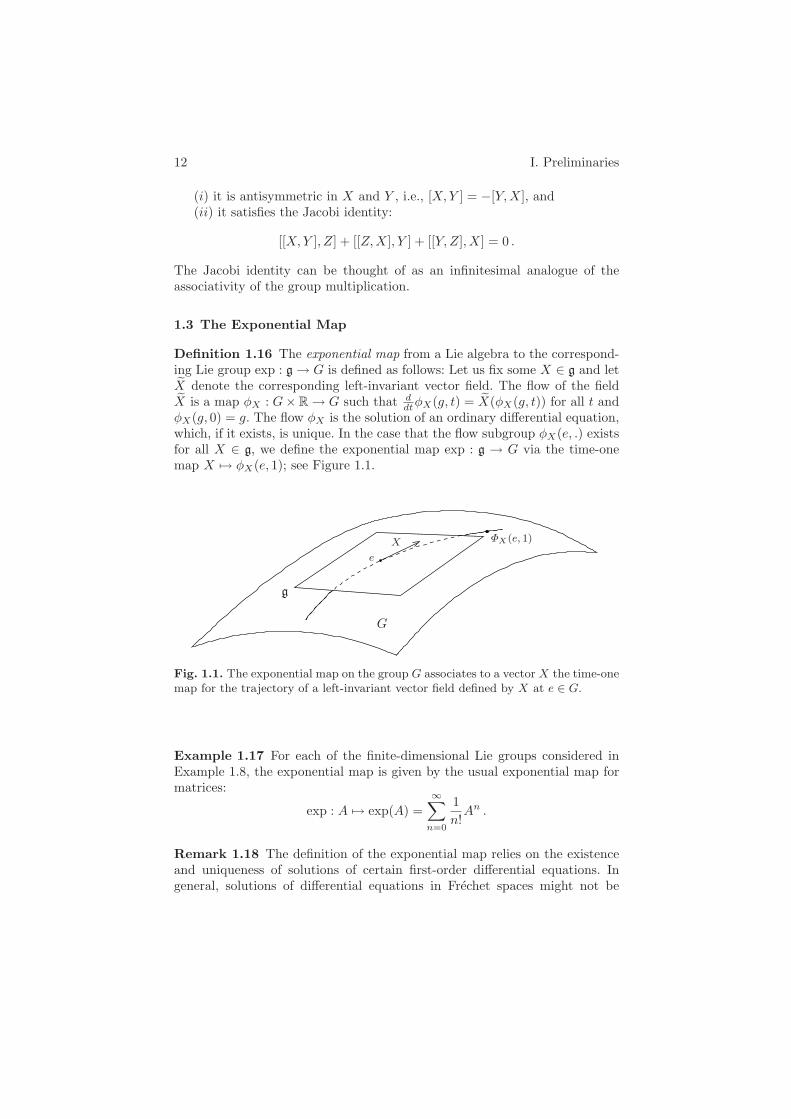
dtφX(g, t) = ˜X(φX(g, t)) for all t andφX(g, 0) = g. The flow φX is the solution of an ordinary differential equation,which, if it exists, is unique. In the case that the flow subgroup φX(e, .) existsfor all X ∈ g, we define the exponential map exp : g → G via the time-onemap X → φX(e, 1); see Figure 1.1.
G
g
ΦX(e, 1)
e
X
Fig. 1.1. The exponential map on the group G associates to a vector X the time-onemap for the trajectory of a left-invariant vector field defined by X at e ∈ G.
Example 1.17 For each of the finite-dimensional Lie groups considered inExample 1.8, the exponential map is given by the usual exponential map formatrices:
exp : A → exp(A) =∞∑
n=0
1n!An .
Remark 1.18 The definition of the exponential map relies on the existenceand uniqueness of solutions of certain first-order differential equations. Ingeneral, solutions of differential equations in Frechet spaces might not be
1. Lie Groups and Lie Algebras 13
unique.3 However, the differential equation in the definition of the exponentialmap is of special type, which secures the solution’s uniqueness upon fixing itsinitial condition. Namely, let φ : R → G be a smooth path in the Lie groupG. Its derivative φ′(t) := d
dtφ(t) is a tangent vector to the group G at thepoint φ(t). Translate this vector back to the identity via left multiplicationby φ−1(t). The corresponding element of the Lie algebra g is denoted byφ−1(t)φ′(t) and is called the left logarithmic derivative of the path φ.
Now consider a Lie algebra element X ∈ g. By definition of the exponentialmap, the curve φ(t) = exp(tX) satisfies the differential equation φ′(t) = φ(t)Xwith the initial condition φ(0) = e. So for all solutions of this differential equa-tion, the left logarithmic derivative is given by the constant curve X ∈ g. Nowthe uniqueness of the exponential map is implied by the following Exercise.
Exercise 1.19 Show that two smooth paths φ, ψ : R → G have the same leftlogarithmic derivative for all t ∈ R if and only if they are translations of eachother by some constant element g ∈ G: φ(t) = g ψ(t) for all t ∈ R. (Hint: see,e.g., [265].)
Remark 1.20 As far as the existence is concerned, the exponential map ex-ists for all finite-dimensional Lie groups and more generally for Lie groupsmodeled on Banach spaces, as follows from the general theory of differentialequations. However, there may exist infinite-dimensional Lie groups that donot admit an exponential map. Moreover, even in the cases in which the ex-ponential map of an infinite-dimensional group exists, it can exhibit ratherpeculiar properties; see the examples below.
Example 1.21 For the diffeomorphism group Diff(M) the exponential mapexp : Vect(M) → Diff(M) has to assign to each vector field on M the time-onemap for its flow. However, for a noncompact M this map may not exist: thecorresponding vector field may not be complete. Indeed, for example, for thevector field ξ = x2∂/∂x on the real line M = R, the time-one map of the flowis not defined on the whole of R: the corresponding flow sends some points toinfinity for the time less than 1! Fortunately, for compact manifolds M andsmooth vector fields, the time-one maps of the corresponding flows, and hencethe exponential maps, are well defined.
Note that the group of diffeomorphisms of a noncompact manifold is notcomplete, and hence it is not a Lie group in our sense. It is an important openproblem to find a Lie group that is modeled on a complete space and doesnot admit an exponential map.3 For instance, the initial value problem u(x, 0) = f(x) for the equation ut(x, t) =
ux(x, t) with x ∈ [0, 1] has wave-type solutions u(x, t) = f(x + t). For nonzerot such a solution u(x, t) for x ∈ [0, 1] depends on the extension of f(x) to thesegment [−t, 1− t]. Due to arbitrariness in the choice of a smooth extension of ffrom [0, 1] to R, the solution to this initial value problem is not unique.

14 I. Preliminaries
Let us return to the current group GM , where the exponential map existsand can be used to give this group the structure of a Frechet Lie group.Namely, the space gM = C∞(M, g) endowed with the topology of uniformconvergence is a Frechet space. Moreover, the map exp : g → G can be used todefine a map exp : gM → GM pointwise. In a sufficiently small neighborhoodof 0 ∈ gM , the map exp is bijective. Thus it can be used to define a local systemof open neighborhoods of the identity in GM . We can use left translation totransfer this system to any point in GM and thus define a topology on thegroup GM . Again using the exponential map, we can define coordinate chartson GM . This definition implies that multiplication and inversion in GM aresmooth maps. So GM is an infinite-dimensional Lie groups (see, e.g., [157] formore details).
From the construction of the Lie group structure on GM , it is clear that itsLie algebra is the current algebra gM , and that the exponential map gM → GM
is the map exp described above. Note, however, that exp is not, in general,surjective, even if exp : g → G is surjective. As an example, take the manifoldM to be the circle S1 and G to be the group SU(2).
Exercise 1.22 Show that the map
θ →(
eiθ 00 e−iθ
)
for θ ∈ S1 = R/2πZ defines an element in GS1that does not belong to the
image of the exponential map exp : gS1 → GS1.
In contrast to the exponential map in the case of the current group GM ,the exponential map exp : Vect(M) → Diff(M) for the diffeomorphism groupof a compact M is not, in general, even locally surjective already for the caseof a circle.
Proposition 1.23 (see, e.g., [265, 301, 322]) The exponential map exp :Vect(S1) → Diff(S1) is not locally surjective.
Proof. First observe that any nowhere-vanishing vector field on S1 is conju-gate under Diff(S1) to a constant vector field. Indeed, if ξ(θ) = v(θ) ∂
∂θ is such avector field, we can define a diffeomorphism ψ : S1 → S1 via ψ(θ) = a
∫ θ
0dt
v(t) .Here, a ∈ R is chosen such that ψ(2π) = 2π. Then ψ∗(ξ ψ−1) is a constantvector field on S1.
From this observation, one can conclude that any diffeomorphism of S1
that lies in the image of the exponential map and that does not have anyfixed points is conjugate to a rigid rotation of S1. Hence in order to see thatthe exponential map is not locally surjective, it is enough to construct diffeo-morphisms arbitrarily close to the identity that do not have any fixed points
1. Lie Groups and Lie Algebras 15
and that are not conjugate to a rigid rotation. For this, one can take dif-feomorphisms without fixed points, but which have isolated periodic points,i.e., fixed points for a certain nth iteration of this diffeomorphism. Indeed, ifsuch a diffeomorphism ψ belonged to the image of the exponential map, sowould its nth power ψn. Then the corresponding vector field defining the ψn
as the time-one map would either have zeros or be nonvanishing everywhere.In the former case, the n-periodic points of ψ must actually be its fixed points,while in the latter case, the diffeomorphism ψn, as well as ψ, would be conju-gate to a rigid rotation and hence all points of ψ would be n-periodic. Bothcases give us a contradiction.
Explicitly, a family of such diffeomorphisms can be constructed as follows:Let us identify S1 with R/2πZ. Then consider the map ψn,ε : x → x +2πn + ε sin(nx). For ε small enough, this is indeed a diffeomorphism of S1.Furthermore, by choosing n large and ε small, the diffeomorphisms ψn,ε canbe made arbitrarily close to the identity while having no fixed points. Finally,for ε = 0, ψn,ε cannot be conjugate to a rigid rotation. If it were conjugateto a rotation, it would have to be the rotation ψn,0, since ψn
n,ε(0) = 0. But inthis case, we would have ψn
n,ε = id, which is not true for ε = 0.
1.4 Abstract Lie Algebras
As we have seen in the last section, the Lie bracket of two left-invariant vectorfields ˜X and ˜Y on a Lie group G defines a bilinear map [ . , . ] : g × g → g ofthe Lie algebra of G that is antisymmetric in X and Y and satisfies the Jacobiidentity (1.2). These properties can be taken as the definition of an abstractLie algebra:
Definition 1.24 An (abstract) Lie algebra is a real or complex vector spaceg together with a bilinear map [ . , . ] : g × g → g (the Lie bracket) that isantisymmetric in X and Y and that satisfies the Jacobi identity
[[X,Y ], Z] + [[Z,X], Y ] + [[Y,Z],X] = 0 . (1.2)
All the Lie algebras we have encountered so far as accompanying the cor-responding Lie groups can also be regarded by themselves, i.e., as abstract Liealgebras. A famous theorem of Sophus Lie states that every finite-dimensional(abstract) Lie algebra g is the Lie algebra of some Lie group G. In infinitedimensions this is no longer true in general.
Example 1.25 ([205, 207]) To illustrate the failure of Lie’s theorem in aninfinite-dimensional context, consider the Lie algebra of complex vector fieldson the circle VectC(S1) = Vect(S1) ⊗ C. Let us show that this Lie algebracannot be the Lie algebra of any Lie group. First note that VectC(S1) contains

16 I. Preliminaries
as a subalgebra the Lie algebra Vect(S1) of real vector fields on the circle,which is the Lie algebra of the group Diff(S1).
Let G1 denote the group PSL(2,R) and let Gk denote the k-fold coveringof G1. The group G2 is isomorphic to SL(2,R), while for k > 2 it is knownthat the groups Gk have no matrix realization. The group Diff(S1) containseach Gk as a subgroup. Namely, Gk is the subgroup corresponding to the Liesubalgebra gk spanned by the vector fields
∂
∂θ, sin(kθ)
∂
∂θ, cos(kθ)
∂
∂θ.
(Note that each gk is isomorphic to sl(2,R).)Now suppose that there exists a complexification of the group Diff(S1),
i.e., a Lie group G corresponding to the complex Lie algebra VectC(S1). Sucha group G would have to contain the complexifications of all the groups Gk.However, for k > 2 the groups Gk do not admit complexifications: the onlycomplex groups corresponding to the Lie algebra sl(2,C) are SL(2,C) andPSL(2,C).
More precisely, if the complex Lie group G existed, the real subgroupsGk would belong to the complex subgroups of G corresponding to complexsubalgebras gC
k sl(2,C). But these complex subgroups have to be isomorphiceither to SL(2,C), which contains only SL(2,R) = G2, or to PSL(2,C), whichcontains only PSL(2,R) = G1. Thus the complex group G containing all Gk
cannot exist, and hence there is no Lie group for the Lie algebra VectC(S1).
Lie algebra homomorphisms are defined in the usual way: A map ρ : g → h
between two Lie algebras is a Lie algebra homomorphism if it satisfiesρ([X,Y ]) = [ρ(X), ρ(Y )] for all X, Y ∈ g. We will also need another im-portant class of maps between Lie algebras called derivations:
Definition 1.26 A linear map δ : g → g of a Lie algebra g to itself is calleda derivation if it satisfies
δ([X,Y ]) = [δ(X), Y ] + [X, δ(Y )]
for all X, Y ∈ g.
Exercise 1.27 Define the map adX : g → g associated to a fixed vectorX ∈ g via
adX(Y ) = [X,Y ] .
Show that this is a derivation for any choice of X. (Hint: use the Jacobiidentity.)
If a derivation of a Lie algebra g can be expressed in the form adX for someX ∈ g, it is called an inner derivation; otherwise, it is called an outer deriva-tion of g.
2. Adjoint and Coadjoint Orbits 17
Exercise 1.28 Let δ be a derivation of a Lie algebra g, and suppose thatexp(δ) =
∑∞i=0
1i!δ
i makes sense (for example, suppose, the map δ is nilpotent).Show that the map exp(δ) is an automorphism of the Lie algebra g.
Definition 1.29 A subalgebra of a Lie algebra g is a subspace h ⊂ g invariantunder the Lie bracket in g. An ideal of a Lie algebra g is a subalgebra h ⊂ g
such that [X, h] ⊂ h for all X ∈ g.
The importance of ideals comes from the fact that if h ⊂ g is an ideal,then the quotient space g/h is again a Lie algebra.
Exercise 1.30 (i) Show that for an ideal h ⊂ g the Lie bracket on g descendsto a Lie bracket on the quotient space g/h.
(ii) Show that if ρ : g → g is a homomorphism of two Lie algebras, thenthe kernel ker ρ of ρ is an ideal in g.
Definition 1.31 A Lie algebra is simple (respectively, semisimple) if it doesnot contain nontrivial ideals (respectively, nontrivial abelian ideals).
Any finite-dimensional semisimple Lie algebra is a direct sum of nonabeliansimple Lie algebras.
A group analogue of an ideal is the notion of a normal subgroup. A sub-group H ⊂ G of a group G is called normal if gHg−1 ⊂ H for all g ∈ G.Exercise 1.30 translates directly to normal subgroups.
2 Adjoint and Coadjoint Orbits
Writing out a linear operator in a different basis or a vector field in a differentcoordinate system has a far-reaching generalization as the adjoint represen-tation for any Lie group. In this section we define the adjoint and coadjointrepresentations and the corresponding orbits for an arbitrary Lie group.
2.1 The Adjoint Representation
A representation of a Lie group G on a vector space V is a linear action ϕof the group G on V that is smooth in the sense that the map G × V →V , (g, v) → gv, is smooth. If V is a real vector space, (V, ϕ) is called a realrepresentation, and if V is complex, it is a complex representation. (Here V isassumed to be a Frechet space, and, often, a Hilbert space. In the latter case,the representation is said to be unitary if the inner product on V is invariantunder the action of G.)
18 I. Preliminaries
Every Lie group has two distinguished representations: the adjoint and thecoadjoint representations. Since they will play a special role in this book, wedescribe them in more detail.
Any element g ∈ G defines an automorphism cg of the group G by conju-gation:
cg : h ∈ G → ghg−1.
The differential of cg at the identity e ∈ G maps the Lie algebra of G to itselfand thus defines an element Adg ∈ Aut(g), the group of all automorphisms ofthe Lie algebra g.
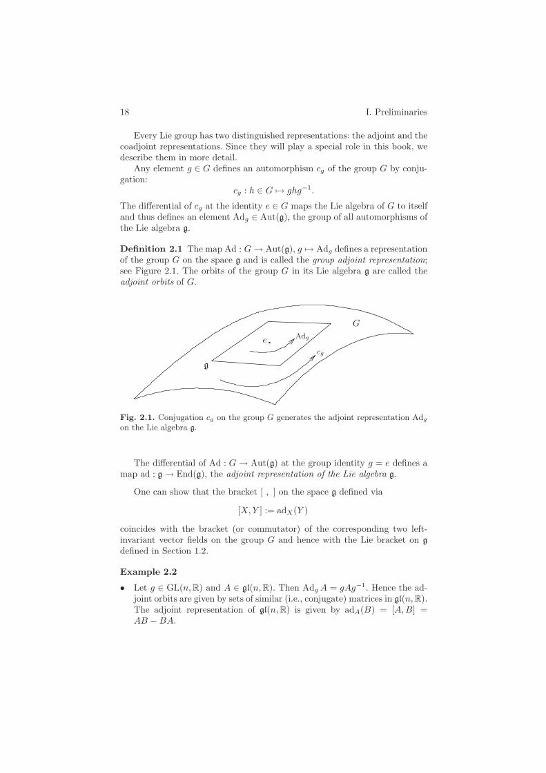
Definition 2.1 The map Ad : G → Aut(g), g → Adg defines a representationof the group G on the space g and is called the group adjoint representation;see Figure 2.1. The orbits of the group G in its Lie algebra g are called theadjoint orbits of G.
G
g
Adg
cg
e
Fig. 2.1. Conjugation cg on the group G generates the adjoint representation Adg
on the Lie algebra g.
The differential of Ad : G → Aut(g) at the group identity g = e defines amap ad : g → End(g), the adjoint representation of the Lie algebra g.
One can show that the bracket [ , ] on the space g defined via
[X,Y ] := adX(Y )
coincides with the bracket (or commutator) of the corresponding two left-invariant vector fields on the group G and hence with the Lie bracket on g
defined in Section 1.2.
Example 2.2
• Let g ∈ GL(n,R) and A ∈ gl(n,R). Then Adg A = gAg−1. Hence the ad-joint orbits are given by sets of similar (i.e., conjugate) matrices in gl(n,R).The adjoint representation of gl(n,R) is given by adA(B) = [A,B] =AB −BA.

2. Adjoint and Coadjoint Orbits 19
• The adjoint orbits of SO(3,R) are spheres centered at the origin of R3
so(3,R) and the origin itself.• The adjoint orbits of SL(2,R) are contained in the sets of similar matrices.
By writing A =(
a bc −a
)
∈ sl(2,R), one sees that the adjoint orbits lie inthe level sets of ∆ = −(a2 + bc) = const: matrices that are conjugateto each other have the same determinant. Note, however, that not allmatrices in sl(2,R) that have the same determinant are conjugate. Forinstance, the matrices with determinant ∆ = 0 constitute three differentorbits: the origin and two other orbits, cones, passing through the matrices(
0 ±10 0
)
, respectively. For ∆ = 0 the SL(2,R)-orbits are either one-sheethyperboloids or connected components of the two-sheet hyperboloids a2 +bc = const, since the group SL(2,R) is connected.
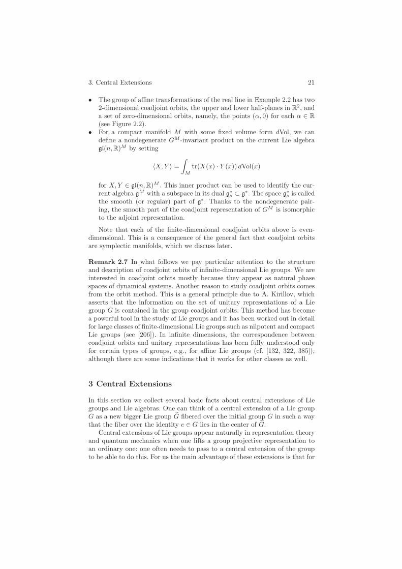
• Let G be the set of orientation-preserving affine transformations of thereal line. That is, G = (a, b) | a, b ∈ R , a > 0, and (a, b) ∈ G acts onx ∈ R via x → ax + b. The Lie algebra of G is R
2, and its adjoint orbitsare the affine lines
(α, β) ∈ R2 | α = const = 0, β arbitrary ,
the two rays
(α, β) ∈ R2, α = 0, β < 0 and (α, β) ∈ R
2, α = 0, β > 0 ,
and the origin (0, 0); see Figure 2.2.• Let M be a compact manifold. The adjoint orbits of the current group
GL(n,C)M in its Lie algebra gl(n,C)M are given by fixing the (smoothlydependent) Jordan normal form of the current at each point of the mani-fold M .
• Let M be a compact manifold. The adjoint representation of Diff(M) onVect(M) is given by coordinate changes of the vector field: for a φ ∈Diff(M) one has Adφ : v → φ∗v φ−1. The adjoint representation ofVect(M) on itself is given by the negative of the usual Lie bracket ofvector fields: adv w = ∂v
∂xw(x) − ∂w∂x v(x) in any local coordinate x.
Exercise 2.3 Verify the latter formula for the action of Diff(M) on Vect(M)from the definition of the group adjoint action. (Hint: express the diffeomor-phisms corresponding to the vector fields v(x) and w(x) in the form
g(t) : x → x+ tv(x) + o(t), h(s) : x → x+ sw(x) + o(s), t, s → 0,
and find the first several terms of g(t)h(s)g−1(t).)
2.2 The Coadjoint Representation
The dual object to the adjoint representation of a Lie group G on itsLie algebra g is called the coadjoint representation of G on g∗, the dualspace to g.

20 I. Preliminaries
®®
¯¯
Fig. 2.2. Adjoint and coadjoint orbits of the group of affine transformations on theline.
Definition 2.4 The coadjoint representation Ad∗ of the group G on thespace g∗ is the dual of the adjoint representation. Let 〈 , 〉 denote the pairingbetween g and its dual g∗. Then the coadjoint action of the group G on thedual space g∗ is given by the operators Ad∗
g : g∗ → g∗ for any g ∈ G that aredefined by the relation
〈Ad∗g(ξ),X〉 := 〈ξ,Adg−1(X)〉 (2.3)
for all ξ in g∗ and X ∈ g. The orbits of the group G under this action on g∗
are called the coadjoint orbits of G.The differential ad∗ : g → End(g∗) of the group representation Ad∗ : G →
Aut(g∗) at the group identity e ∈ G is called the coadjoint representationof the Lie algebra g. Explicitly, at a given vector Z ∈ g it is defined by therelation
〈ad∗Z(ξ),X〉 = −〈ξ, adZ(X)〉.
Remark 2.5 The dual space of a Frechet space is not necessarily again aFrechet space. In this case, instead of considering the full dual space to aninfinite-dimensional Lie algebra g, we will usually confine ourselves to con-sidering only appropriate “smooth duals,” the functionals from a certain G-invariant Frechet subspace g∗s ⊂ g∗. Natural smooth duals will be differentaccording to the type of the infinite-dimensional groups considered, but theyall have a (weak) nondegenerate pairing with the corresponding Lie algebra g
in the following sense: for every nonzero element X ∈ g, there exists some ele-ment ξ ∈ g∗s such that 〈ξ,X〉 = 0, and the other way around. This ensures thatthe coadjoint action is uniquely fixed by equation (2.3). The pair (g∗s,Ad∗ |g∗
s)
is called the regular (or smooth) part of the coadjoint representation of G,and, abusing notations, we will usually skip the index s.
Example 2.6
• In the first three cases of Example 2.2, there exists a G-invariant innerproduct on g that induces an isomorphism between g and g∗ respectingthe group actions. Hence the adjoint and coadjoint representations of thegroups G are isomorphic, and the coadjoint orbits coincide with the adjointones.
3. Central Extensions 21
• The group of affine transformations of the real line in Example 2.2 has two2-dimensional coadjoint orbits, the upper and lower half-planes in R
2, anda set of zero-dimensional orbits, namely, the points (α, 0) for each α ∈ R
(see Figure 2.2).• For a compact manifold M with some fixed volume form dVol, we can
define a nondegenerate GM -invariant product on the current Lie algebragl(n,R)M by setting
〈X,Y 〉 =∫
M
tr(X(x) · Y (x)) dVol(x)
for X,Y ∈ gl(n,R)M . This inner product can be used to identify the cur-rent algebra gM with a subspace in its dual g∗s ⊂ g∗. The space g∗s is calledthe smooth (or regular) part of g∗. Thanks to the nondegenerate pair-ing, the smooth part of the coadjoint representation of GM is isomorphicto the adjoint representation.
Note that each of the finite-dimensional coadjoint orbits above is even-dimensional. This is a consequence of the general fact that coadjoint orbitsare symplectic manifolds, which we discuss later.
Remark 2.7 In what follows we pay particular attention to the structureand description of coadjoint orbits of infinite-dimensional Lie groups. We areinterested in coadjoint orbits mostly because they appear as natural phasespaces of dynamical systems. Another reason to study coadjoint orbits comesfrom the orbit method. This is a general principle due to A. Kirillov, whichasserts that the information on the set of unitary representations of a Liegroup G is contained in the group coadjoint orbits. This method has becomea powerful tool in the study of Lie groups and it has been worked out in detailfor large classes of finite-dimensional Lie groups such as nilpotent and compactLie groups (see [206]). In infinite dimensions, the correspondence betweencoadjoint orbits and unitary representations has been fully understood onlyfor certain types of groups, e.g., for affine Lie groups (cf. [132, 322, 385]),although there are some indications that it works for other classes as well.
3 Central Extensions
In this section we collect several basic facts about central extensions of Liegroups and Lie algebras. One can think of a central extension of a Lie groupG as a new bigger Lie group ˜G fibered over the initial group G in such a waythat the fiber over the identity e ∈ G lies in the center of ˜G.
Central extensions of Lie groups appear naturally in representation theoryand quantum mechanics when one lifts a group projective representation toan ordinary one: one often needs to pass to a central extension of the groupto be able to do this. For us the main advantage of these extensions is that for

22 I. Preliminaries
many infinite-dimensional groups their central extensions have simpler and“more regular” structure of the coadjoint orbits, as well as more interestingdynamical systems related to them.
3.1 Lie Algebra Central Extensions
Definition 3.1 A central extension of a Lie algebra g by a vector space n isa Lie algebra g whose underlying vector space g = g⊕ n is equipped with thefollowing Lie bracket:
[(X,u), (Y, v)]∼ = ([X,Y ], ω(X,Y ))
for some continuous bilinear map ω : g×g → n. (Note that ω depends only onX and Y , but not on u and v, which means that the extension is central: thespace n belongs to the center of the new Lie algebra, i.e., it commutes withall of g: [(0, u), (Y, v)] = 0 for all Y ∈ g and u, v ∈ n.) The skew symmetryand the Jacobi identity for the new Lie bracket on g are equivalent to thefollowing conditions on the map ω. Such a map ω : g × g → n has to be a2-cocycle on the Lie algebra g, i.e., ω has to be bilinear and antisymmetric,and it has to satisfy the cocycle identity
ω([X,Y ], Z) + ω([Z,X], Y ) + ω([Y,Z],X) = 0
for any triple of elements X,Y,Z ∈ g. (Here and below we always require Liealgebra cocycles to be continuous maps.)
A 2-cocycle ω on g with values in n is called a 2-coboundary if there existsa linear map α : g → n such that ω(X,Y ) = α([X,Y ]) for all X,Y ∈ g. Onecan easily see that the central extension defined by such a 2-coboundary be-comes the trivial extension by the zero cocycle after the change of coordinates(X,u) → (X,u− α(X)).
Hence in describing different central extensions we are interested only inthe 2-cocycles modulo 2-coboundaries, i.e., in the second cohomology H2(g; n)of the Lie algebra g with values in n: H2(g; n) = Z(g; n)/B(g; n), where Z(g; n)is the vector space of all 2-cocycles on g with values in n, and B(g; n) is thesubspace of 2-coboundaries.
Remark 3.2 A central extension of a Lie algebra g by an abelian Lie algebran can be defined by the exact sequence
0 −→ n−→g−→g −→ 0
of Lie algebras such that n lies in the center of g. A morphism of two centralextensions is a pair (ν, µ) of Lie algebra homomorphisms ν : n → n′ andµ : g → g′ such that the following diagram is commutative:
0 −→ n −→ gπ−→ g −→ 0
ν
µ
id
0 −→ n′ −→ g′π′−→ g −→ 0.
(3.4)

3. Central Extensions 23
Two extensions are said to be equivalent if the map µ is an isomorphism andν = id.
Exercise 3.3 Prove the following equivalence:
Proposition 3.4 There is a one-to-one correspondence between the equiva-lence classes of central extensions of g by n and the elements of H2(g; n).
Example 3.5 Consider the abelian Lie algebra g = R2, and let ω ∈ Λ2(R2)
be an arbitrary skew-symmetric bilinear form on R2. Then ω defines a 2-
cocycle on R2 with values in R (in this case, the cocycle condition is triv-
ial, since g is abelian). The resulting central extension is g = R2 ⊕ R with
Lie bracket [(v1, h1), (v2, h2)] = (0, ω(v1, v2)). Moreover, since g is abelian,B(g; R) = 0 whence H2(g; R) = Λ2(R2) ∼= R. Note that all ω = 0 ∈ Λ2(R2)lead to isomorphic Lie algebras. The algebra g with a nonzero ω, i.e., a repre-sentative of this isomorphism class, is called the three-dimensional Heisenbergalgebra.
By taking a nondegenerate skew-symmetric form ω in R2n, we can define
in the same way the (2n+ 1)-dimensional Heisenberg algebra.An infinite-dimensional analogue of the Heisenberg algebra is as follows.
Consider the space g = f ∈ C∞(S1) |∫
S1 f dθ = 0 of smooth functions onthe circle with zero mean and regard it as an abelian Lie algebra. Define the2-cocycle by ω(f, g) =
∫
S1 f ′g dθ. (One can view this algebra and the corre-sponding cocycle as the “limit” n → ∞ of the example above by consideringthe functions in Fourier components.)
Exercise 3.6 Check the skew-symmetry and the cocycle identity for ω(f, g).
Definition 3.7 A central extension g of g is called universal if for any othercentral extension g′, there is a unique morphism g → g′ of the central exten-sions. If it exists, the universal central extension of a Lie algebra g is uniqueup to isomorphism.
Remark 3.8 A sufficient condition for a Lie algebra g to have a universalcentral extension is that g be perfect, i.e., that it coincide with its own de-rived algebra: g = [g, g] (see, e.g., [276]). Any finite-dimensional semisimpleLie algebra is perfect. The universal central extension of a semisimple Lie al-gebra g coincides with g itself: such algebras do not admit nontrivial centralextensions.
No abelian Lie algebra is perfect. Nevertheless, abelian Lie algebras canstill have universal central extensions: for instance, the three-dimensionalHeisenberg algebra is the universal central extension of the abelianalgebra R
2.
24 I. Preliminaries
Example 3.9 Let M be a finite-dimensional manifold. One can show thatthe Lie algebra Vect(M) of vector fields on M is perfect. The universal centralextension of Vect(M) for the case M = S1 is called the Virasoro algebra, andwe describe it in detail in Section 2 of Chapter II.
Example 3.10 For a simple Lie algebra g and any n-dimensional compactmanifold M , the current Lie algebra gM is perfect. (More generally, for anyperfect finite-dimensional Lie algebra g the Lie algebra gM is perfect.) Itsuniversal central extension gM can be constructed as follows. Let 〈 , 〉 be anondegenerate symmetric invariant bilinear form on g, where the invariancemeans that 〈[A,B], C〉 = 〈A, [B,C]〉 for all A, B, C ∈ g. Denote by Ω1(M)the set of 1-forms on M and let dΩ0(M) be the subset of exact 1-forms. Nowwe define the 2-cocycle ω on gM with values in Ω1(M)/dΩ0(M) via
ω(X,Y ) := 〈X, dY 〉 ,
where X, Y ∈ gM . The antisymmetry of ω is immediate, while the cocycleidentity follows from the Jacobi identity in gM and the invariance of thebilinear form. So ω defines a central extension of gM . For a proof of universalityof this central extension see, e.g., [322, 247].
In the case of M = S1 the corresponding space Ω1(S1)/dΩ0(S1) is one-dimensional. The current algebra on S1 is called the loop algebra associated tog, and it has the universal central extension by the R- (or C)-valued 2-cocycle
ω(X,Y ) :=∫
S1〈X, dY 〉 .
We discuss loop algebras and their generalizations in detail in Sections 1 and5 of Chapter II.
3.2 Central Extensions of Lie Groups
Central extensions of Lie groups can be defined similarly to those of Lie al-gebras. However, unlike the case of Lie algebras, not all group extensions canbe described explicitly by cocycles. This is why we start with the alternativedefinition of the extensions via exact sequences.
Definition 3.11 A central extension ˜G of a Lie group G by an abelian Liegroup H is an exact sequence of Lie groups
e → H → ˜G → G → e
such that the image of H lies in the center of ˜G. (Here e is the trivialgroup containing only the identity element.) Morphisms and equivalence oftwo central extensions are defined analogously to the case of Lie algebras.
3. Central Extensions 25
If the central extension ˜G is topologically a direct product of G and H,˜G = G × H (or, equivalently, if there is a smooth section in the principalH-bundle ˜G → G),4 one can define the multiplication in ˜G as follows:
(g1, h1) · (g2, h2) = (g1g2, γ(g1, g2)h1h2)
for a smooth map γ : G×G → H, which is similar to the case of Lie algebracentral extensions. The associativity of this multiplication corresponds to theso-called group cocycle identity on the map γ.
Definition 3.12 Let G and H be Lie groups and suppose H is abelian. Asmooth map γ : G×G → H that satisfies
γ(g1g2, g3)γ(g1, g2) = γ(g1, g2g3)γ(g2, g3)
is called a smooth group 2-cocycle on G with values in H.A smooth 2-cocycle on G with values in H is called a 2-coboundary if there
exists a smooth map λ : G → H such that γ(g1, g2) = λ(g1)λ(g2)λ(g1g2)−1. Asbefore, the group 2-coboundaries correspond to the trivial group extensions,after a possible change of coordinates (more precisely, of the trivializing sectionfor ˜G → G). Similarly, two group 2-cocycles define isomorphic extensions ifthey differ by a 2-coboundary. This explains the following fact.
Proposition 3.13 There is a one-to-one correspondence between the set ofcentral extensions of G by H that admit a smooth section and the ele-ments in the second cohomology group H2(G,H) := Z(G,H)/B(G,H). HereZ(G,H) and B(G,H) denote respectively the sets of smooth 2-cocycles and2-coboundaries on G, with the natural abelian group structure.
However, in contrast to the case of Lie algebras, there exist central exten-sions of Lie groups that do not admit a smooth section, and hence cannot bedefined by smooth 2-cocycles. We will encounter examples for such groups inChapter II.
A central extension of a Lie group G always defines a central extension ofthe corresponding Lie algebra. The converse need not be true: the existenceof a Lie group for a given Lie algebra is not guaranteed in infinite dimensions.Instead, one says that a central extension g of a Lie algebra g lifts to thegroup level if there exists a central extension ˜G of the group G whose Liealgebra is given by g. If the group central extension ˜G by H is defined bya group 2-cocycle γ, one can recover the Lie algebra 2-cocycle defining thecorresponding central extension g of the Lie algebra g directly from the groupcocycle γ by appropriate differentiation.4 We always require central extensions of Lie groups to have smooth local sections,
in order to secure the existence of a continuous linear section for the correspondingLie algebra extensions.
26 I. Preliminaries
Proposition 3.14 Let H be an abelian Lie group with a Lie algebra h, andlet γ be an H-valued 2-cocycle on G defining a central extension ˜G. Then theh-valued 2-cocycle ω defining the corresponding central extension g of the Liealgebra g is given by
ω(X,Y ) =d2
dt ds
∣
∣
∣
t=0,s=0γ(gt, hs) −
d2
dt ds
∣
∣
∣
t=0,s=0γ(hs, gt) ,
where gt is a smooth curve in G such that ddt |t=0gt = X, and hs is a smooth
curve in G such that dds |s=0hs = Y .
Exercise 3.15 Prove the above proposition.
Example 3.16 Let G be R2 = (a, b) with the natural abelian group struc-
ture. The three-dimensional Heisenberg group ˜G can be defined as the follow-ing matrix group:
˜G =
⎧
⎨
⎩
⎛
⎝
1 a c0 1 b0 0 1
⎞
⎠ | a, b, c ∈ R
⎫
⎬
⎭
,
and it is a central extension of the group G. One verifies directly that thecentral extension is defined via the R-valued group 2-cocycle γ given byγ((a, b), (a′, b′)) = ab′. Using Proposition 3.14, we see that the infinitesimalform of the cocycle γ is given by
ω((A,B), (A′, B′)) = AB′ −A′B,
so that the Lie algebra of ˜G is the three-dimensional Heisenberg algebra dis-cussed in Example 3.5.
4 The Euler Equations for Lie Groups
The Euler equations form a class of dynamical systems closely related to Liegroups and to the geometry of their coadjoint orbits. To describe them westart with generalities on Poisson structures and Hamiltonian systems, beforebridging them to Lie groups. Although the manifolds considered in this sectionare finite-dimensional, we will see later in the book that most of the notionsand formulas discussed here are applicable in the infinite-dimensional context(where the dual g∗ of a Lie algebra g stands for its smooth dual).
4.1 Poisson Structures on Manifolds
Definition 4.1 A Poisson structure on a manifold M is a bilinear operationon functions
, : C∞(M) × C∞(M) → C∞(M)

4. The Euler Equations for Lie Groups 27
satisfying the following properties:(i) antisymmetry:
f, g = −g, f,(ii) the Jacobi identity:
f, g, h + g, h, f + h, f, g = 0, and
(iii) the Leibniz identity:
f, gh = f, gh+ f, hg
for any functions f, g, h ∈ C∞(M).
The first two properties mean that a Poisson structure defines a Lie algebrastructure , on the space C∞(M) of smooth functions on M , while thethird property implies that f, · : C∞(M) → C∞(M) is a derivation forany function f ∈ C∞(M). Since each derivation on the space of functions isthe Lie derivative along an appropriate vector field, the Poisson structure canbe thought of as a map from functions to the corresponding vector fields onthe manifold:
Definition 4.2 Let H : M → R be any smooth function on a Poisson mani-fold M . Such a function H defines a vector field ξH on M by LξH
g = H, gfor any test function g ∈ C∞(M). The vector field ξH is called the Hamil-tonian field corresponding to the Hamiltonian function H with respect to thePoisson bracket , .
We call a function F : M → R a Casimir function on a Poisson manifoldM if it generates the zero Hamiltonian field, i.e., if the Poisson bracket of thefunction F with any other function vanishes everywhere on M .
Remark 4.3 Let M be a manifold with a Poisson structure , , and wefix some point m ∈ M . All Hamiltonian vector fields on M evaluated atthe point m ∈ M span a subspace of the tangent space TmM . Thus, thePoisson structure defines a distribution of such subspaces on the manifold M(i.e., a subbundle of the tangent bundle TM) by varying the point m.5 Notethat the dimension of this distribution can differ from one point to another.This distribution is integrable, according to the Frobenius theorem, since thecommutator of two Hamiltonian vector fields is again Hamiltonian. Therefore,it gives rise to a (possibly singular) foliation of the Poisson manifold M [384].
5 Alternatively, a Poisson structure can be defined by specifying a bivector field Πon the manifold M , i.e., a section of TM∧2:
f, g = Π(df, dg).
Such a bivector field defines a distribution on M as the images of the map Π :T ∗M → TM .

28 I. Preliminaries
The leaves of this foliation are called symplectic leaves. (In short, two pointsbelong to the same symplectic leaf if they can be joined by a path whosevelocity at any point is a Hamiltonian vector.)
Definition 4.4 A pair (N,ω) consisting of a manifold N and a 2-form ω onN is called a symplectic manifold if ω is closed (dω = 0) and nondegenerate.(In the case of infinite dimensions, the form ω is required to be nondegeneratein the sense that for each point p ∈ N and any nonzero vector X ∈ TpN ,there exists another vector Y ∈ TpM such that ωp(X,Y ) = 0.) The 2-form ωis called the symplectic form on the manifold N .
The reason for the name “symplectic leaves” in Remark 4.3 is that onecan define a symplectic 2-form ω on each leaf. It suffices to fix its values onHamiltonian vector fields ξf and ξg at any point:
ω(ξf , ξg) := f, g ,
since the tangent space of each leaf is generated by Hamiltonian fields.
Exercise 4.5 Show that the 2-form ω defined on the leaf through a pointm ∈ M is closed and nondegenerate.
Note that Casimir functions, by definition, are constant on the leaves of theabove foliation, and the codimension of generic symplectic leaves on a Pois-son manifold M is equal to the number of (locally functionally) independentCasimir functions on M .
Example 4.6 For the Poisson structure
f, g :=∂f
∂x
∂g
∂y− ∂f
∂y
∂g
∂x
in R3 = (x, y, z), its symplectic leaves are the planes z = const. The coor-
dinate function z, or any function F = F (z), is a Casimir function for thisPoisson manifold.
Remark 4.7 Locally, a Poisson manifold near any point p splits into theproduct of a symplectic space and a Poisson manifold whose rank at p is zero[384]. The symplectic space is a neighborhood of the symplectic leaf passingthrough p, while the Poisson manifold of zero rank represents the transversePoisson structure at the point p.
Below we will see that this splitting works in many (but not all!) infinite-dimensional examples: Poisson structures can have infinite-dimensional sym-plectic leaves and finite-dimensional Poisson transversals.
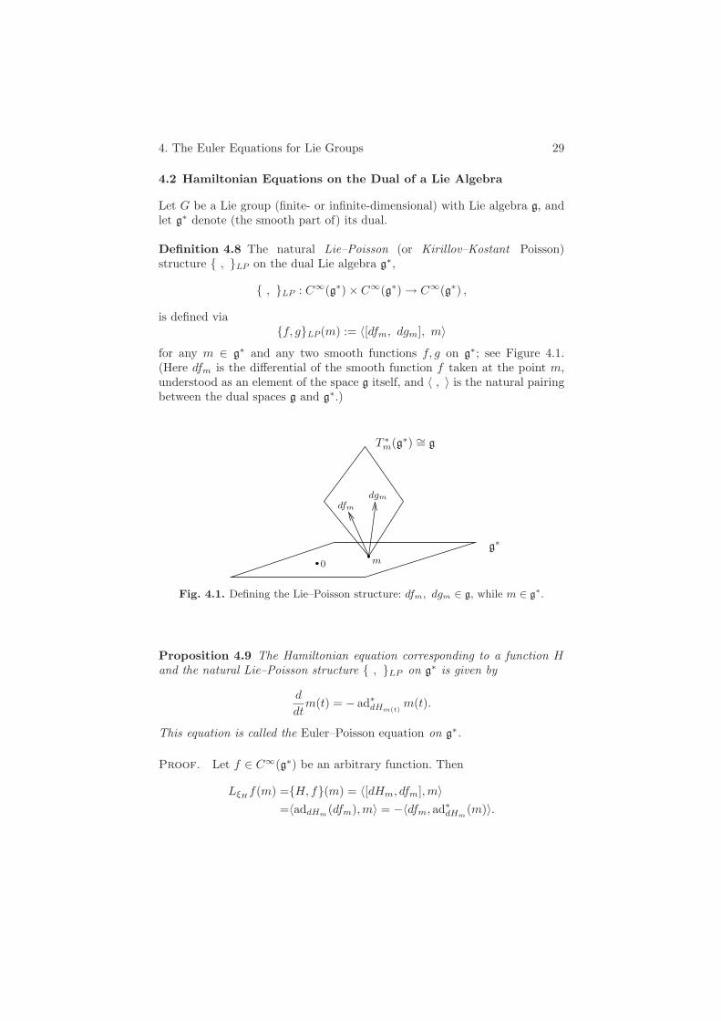
4. The Euler Equations for Lie Groups 29
4.2 Hamiltonian Equations on the Dual of a Lie Algebra
Let G be a Lie group (finite- or infinite-dimensional) with Lie algebra g, andlet g∗ denote (the smooth part of) its dual.
Definition 4.8 The natural Lie–Poisson (or Kirillov–Kostant Poisson)structure , LP on the dual Lie algebra g∗,
, LP : C∞(g∗) × C∞(g∗) → C∞(g∗) ,
is defined viaf, gLP(m) := 〈[dfm, dgm], m〉
for any m ∈ g∗ and any two smooth functions f, g on g∗; see Figure 4.1.(Here dfm is the differential of the smooth function f taken at the point m,understood as an element of the space g itself, and 〈 , 〉 is the natural pairingbetween the dual spaces g and g∗.)
g∗
T ∗m(g∗) ∼= g
dgm
0 m
dfm
Fig. 4.1. Defining the Lie–Poisson structure: dfm, dgm ∈ g, while m ∈ g∗.
Proposition 4.9 The Hamiltonian equation corresponding to a function Hand the natural Lie–Poisson structure , LP on g∗ is given by
d
dtm(t) = − ad∗
dHm(t)m(t).
This equation is called the Euler–Poisson equation on g∗.
Proof. Let f ∈ C∞(g∗) be an arbitrary function. Then
LξHf(m) =H, f(m) = 〈[dHm, dfm],m〉
=〈addHm(dfm),m〉 = −〈dfm, ad∗
dHm(m)〉.
30 I. Preliminaries
Since the Lie derivative of a function f along a vector field is the evaluationof the function’s differential df on this vector field, this implies that ξH(m) =− ad∗
dHm(m), which is the assertion.
Corollary 4.10 The symplectic leaves of , LP on g∗ are the coadjointorbits of G. In particular, all (finite-dimensional) coadjoint orbits have evendimension.
Proof. Denote by Om the coadjoint orbit through a point m ∈ g∗ in thedual space. Let H ∈ C∞(g∗) be a function on the dual. For any vector v ∈ g
of the Lie algebra, one can represent it as v = dHm by taking an appropriatefunction H. Therefore, one can obtain as Hamiltonian vectors ad∗
dHm(m) at
the point m all vectors in the image of ad∗g(m), i.e., all vectors in the tangent
space to the orbit TmOm := Tm(Ad∗G(m)). By definition, all Hamiltonian
vectors span the tangent space to any symplectic leaf at each point m, whichproves that coadjoint orbits are exactly the symplectic leaves of the Lie–Poisson bracket.
Corollary 4.11 Let A : g → g∗ be an invertible self-adjoint operator.6
For the quadratic Hamiltonian function H : g∗ → R defined by H(m) :=12 〈m,A−1m〉 the corresponding Hamiltonian equation is
d
dtm(t) = − ad∗
A−1m(t) m(t) . (4.5)
Indeed, dHm(m) = A−1m for any m ∈ g∗.
Definition 4.12 An invertible self-adjoint operator A : g → g∗ defining thequadratic Hamiltonian H is called an inertia operator on g.
4.3 A Riemannian Approach to the Euler Equations
It turns out that the Euler–Poisson equations with quadratic Hamiltonianshave a beautiful Riemannian reformulation.
V. Arnold suggested in [12] the following general setup for the Euler equa-tion describing a geodesic flow on an arbitrary Lie group. Consider a (possiblyinfinite-dimensional) Lie group G, which can be thought of as the configura-tion space of some physical system. (Examples from [12, 18]: SO(3) for a rigid
6 Note that one can define the “self-adjointness property” for an operator from aspace to its dual, similarly to a self-adjoint operator acting on a given space withrespect to a fixed pairing.
4. The Euler Equations for Lie Groups 31
body or the group SDiff(M) of volume-preserving diffeomorphisms for an idealfluid filling a domain M .) The tangent space at the identity of the Lie groupG is the corresponding Lie algebra g. Fix some (positive definite) quadraticform, the energy, on g. We consider left (or right) translations of this quadraticform to the tangent space at any point of the group (the “translational sym-metry” of the energy). In this way, the energy defines a left- (respectively,right-) invariant Riemannian metric on the group G. The geodesic flow onG with respect to this energy metric represents extremals of the least-actionprinciple, i.e., possible motions of our physical system.7 To describe a geodesicon the Lie group G with an initial velocity v(0), we transport its velocity vec-tor at any moment t to the identity of the group using the left (respectively,right) translation. This way we obtain the evolution law for v(t) on the Liealgebra g.
To fix the notation, let ( , ) be some left-invariant metric on the group G.The geodesic flow with respect to this metric is a dynamical system on thetangent bundle TG of the group G. We can pull back this system to the Liealgebra g of the group G by left translation. That is, if g(t) is a geodesic inthe group G with tangent vector g′(t), then the pullback v(t) = l∗g(t)−1g′(t)is an element of the Lie algebra g. (In the case of a right-invariant metric,we set v(t) = r∗g(t)−1g′(t).) Hence, the geodesic equations for g(t) give us adynamical system
d
dtv(t) = B(v(t)) (4.6)
on the Lie algebra g of the group G, where B : g → g is a (nonlinear) operator.
Definition 4.13 The dynamical system (4.6) on the Lie algebra g describingthe evolution of the velocity vector of a geodesic in a left-invariant metricon the Lie group G is called the Euler (or Euler–Arnold) equation correspon-ding to this metric on G.
It turns out that the Euler equation for a Lie group G can be viewed asa Hamiltonian equation on the dual of the Lie algebra g in the following way.Observe that the metric ( , )e at the identity e ∈ G defines a nondegeneratebilinear form on the Lie algebra g, and therefore, it also determines an inertiaoperator A : g → g∗ such that (v, w)e = 〈A(v), w〉 for all v, w ∈ g. Thisidentification A : g → g∗ allows one to rewrite the Euler equation on the dualspace g∗; see Figure 4.2. Now, setting m = A(v), one can relate the geodesicequation (4.6) on the Lie algebra g to the Hamiltonian equation on the dualg∗ with respect to the Hamiltonian function H(m) = 1
2 〈m,A−1m〉:
7 Usually, the finite-dimensional examples below are related to the left invariance,while the infinite-dimensional ones with the right invariance of the metric. Inparticular, for a rigid body one has to consider left translations on SO(3), whilefor fluids, one must consider the right ones on SDiff(M).

32 I. Preliminaries
G
eg(t)
g
g∗
v
A
m
Fig. 4.2. The vector v in the Lie algebra g traces the evolution of the velocity vectorof a geodesic g(t) on the group. The inertia operator A sends v to a vector m in thedual space g
∗.
Theorem 4.14 (Arnold [12, 13, 18]) For the left-invariant metric on agroup generated by an inertia operator A : g → g∗, the Euler (or the geo-desic) equation (4.6) assumes the form
d
dtm(t) = − ad∗
A−1m(t) m(t)
on the dual space g∗.8
We postpone the proof of this theorem until the end of this section.
Remark 4.15 The underlying reason for the Riemannian reformulation isthe fact that any geodesic problem in Riemannian geometry can be describedin terms of symplectic geometry. Geodesics on M are extremals of a quadraticLagrangian on TM (coming from the metric on M). They can also be de-scribed by the Hamiltonian flow on T ∗M for the quadratic Hamiltonian func-tion obtained from the Lagrangian via the Legendre transform.
If the manifold is a group G with a left-invariant metric, then there existsthe group action on the tangent bundle TG, as well as on the cotangent bundleT ∗G. The left translations on the group trivialize the cotangent bundle T ∗G ∼=G× g∗ and identify any cotangent space of G with g∗. By taking the quotientwith respect to the group action, from the (symplectic) cotangent bundleT ∗G we obtain the dual Lie algebra g∗ = T ∗G|e equipped with the negative
8 Note that these signs are different from the conventions in the book [24], since wehave used a different definition of Ad∗ here (see equation (2.3)) in order to havethe group coadjoint representation, rather than the antirepresentation.
4. The Euler Equations for Lie Groups 33
of the Lie–Poisson structure (cf. Section 5 below, on symplectic reduction).The Hamiltonian function on T ∗G is dual to the Riemannian metric (viewedas a form on TG), and its restriction to g∗ is the quadratic form H(m) =12 〈m,A−1m〉, where m ∈ g∗.
The geodesics of a left-invariant metric on G correspond to the Hamil-tonian function H(m) with respect to the standard Lie–Poisson structure.
Remark 4.16 Instead of using a left-invariant metric on G, we could haveused a right-invariant one. This changes the signs in the Euler equation, sothat one obtains
d
dtm = ad∗A−1m(m) .
Now the geodesics in a right-invariant metric correspond to the Hamiltonian−H(m).
Example 4.17 Let us consider the group SO(3). The Lie algebra so(3) ofSO(3) can be identified with R
3 such that the Lie bracket on g is the crossproduct on R
3: [u, v] = v × u. Let A be a symmetric nondegenerate 3 × 3matrix, which we view as an inertia operator for a left-invariant metric onSO(3). Then by Arnold’s theorem, the Euler equation on so(3)∗ is given by
d
dtm = m×A−1m.
For A = diag(I1, I2, I3) one obtains the classical Euler equations for a rigidbody in R
3:d
dtmi = (I−1
k − I−1j )mjmk
for (i, j, k) being a cyclic permutation of (1, 2, 3). Similarly, for G = SO(n), oneobtains the Euler equation for a higher-dimensional rigid body (see Remark4.28 below).
Example 4.18 Many other conservative dynamical systems in mathematicalphysics also describe geodesic flows on appropriate Lie groups. In Table 4.1 welist several examples of such systems to emphasize the range of applicationsof this approach. The choice of a group G (column 1) and an energy metricE (column 2) defines the corresponding Euler equations (column 3).
We discuss many of these examples later in the book. There are plentyof other interesting systems that fit into this framework, such as, e.g., thesuper-KdV equation or gas dynamics. This list is by no means complete, andwe refer to [24, 252] for more details.
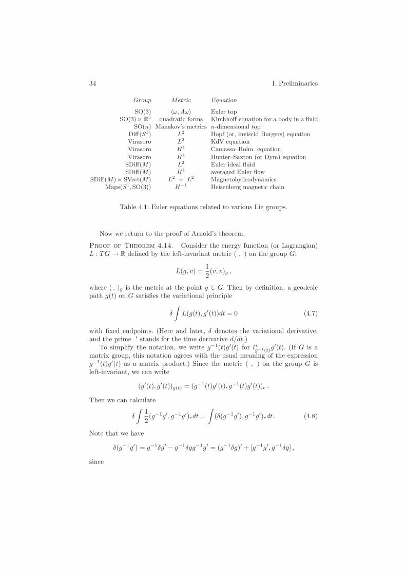
34 I. Preliminaries
Group Metric Equation
SO(3) 〈ω, Aω〉 Euler topSO(3) R
3 quadratic forms Kirchhoff equation for a body in a fluidSO(n) Manakov′s metrics n-dimensional top
Diff(S1) L2 Hopf (or, inviscid Burgers) equationVirasoro L2 KdV equationVirasoro H1 Camassa–Holm equation
Virasoro H1 Hunter–Saxton (or Dym) equationSDiff(M) L2 Euler ideal fluidSDiff(M) H1 averaged Euler flow
SDiff(M) SVect(M) L2 + L2 MagnetohydrodynamicsMaps(S1, SO(3)) H−1 Heisenberg magnetic chain
Table 4.1: Euler equations related to various Lie groups.
Now we return to the proof of Arnold’s theorem.
Proof of Theorem 4.14. Consider the energy function (or Lagrangian)L : TG → R defined by the left-invariant metric ( , ) on the group G:
L(g, v) =12(v, v)g ,
where ( , )g is the metric at the point g ∈ G. Then by definition, a geodesicpath g(t) on G satisfies the variational principle
δ
∫
L(g(t), g′(t))dt = 0 (4.7)
with fixed endpoints. (Here and later, δ denotes the variational derivative,and the prime ′ stands for the time derivative d/dt.)
To simplify the notation, we write g−1(t)g′(t) for l∗g−1(t)g′(t). (If G is a
matrix group, this notation agrees with the usual meaning of the expressiong−1(t)g′(t) as a matrix product.) Since the metric ( , ) on the group G isleft-invariant, we can write
(g′(t), g′(t))g(t) = (g−1(t)g′(t), g−1(t)g′(t))e .
Then we can calculate
δ
∫
12(g−1g′, g−1g′)edt =
∫
(δ(g−1g′), g−1g′)edt . (4.8)
Note that we have
δ(g−1g′) = g−1δg′ − g−1δgg−1g′ = (g−1δg)′ + [g−1g′, g−1δg] ,
since
4. The Euler Equations for Lie Groups 35
(g−1δg)′ = g−1δg′ − g−1g′g−1δg .
Thus, the left-hand-side in equation (4.8) becomes∫
(δ(g−1g′), g−1g′)edt =∫
((g−1δg)′, g−1g′)edt+∫
([g−1g′, g−1δg], g−1g′)edt
= −∫
(g−1δg, (g−1g′)′)edt+∫
([g−1g′, g−1δg], g−1g′)edt ,
where we have used integration by parts in the last step. (Since we confinedourselves to variations of the path g with fixed endpoints, we do not pick upany boundary terms in the integration by parts.)
Now set v(t) := g−1(t)g′(t), and let A : g → g∗ be the inertia operatordefined by the metric ( , )e: (u,w)e = 〈u,Aw〉. Then the right-hand side inthe latter equation becomes
−∫
(g−1δg, (g−1g′)′)edt+∫
([g−1g′, g−1δg], g−1g′)edt
= −∫
〈g−1δg, (Av)′〉dt+∫
〈adv(g−1δg), Av〉dt
= −∫
〈g−1δg, (Av)′〉dt−∫
〈g−1δg, ad∗v(Av)〉dt = 0 .
This implies(Av)′ = − ad∗
v(Av) .
Rewriting this equation in terms of m = Av finishes the proof ofTheorem 4.14.
4.4 Poisson Pairs and Bi-Hamiltonian Structures
A first integral (or a conservation law) for a vector field ξ on a manifold Mis a function on M invariant under the flow of this field. In this section wewill show that if the vector field ξ is a Hamiltonian vector field with respectto two different Poisson structures on the manifold M that are compatible ina certain sense, there is a way of constructing first integrals for such a field.
Definition 4.19 Two Poisson structures , 0 and , 1 on a manifold Mare said to be compatible (or form a Poisson pair) if for every λ ∈ R the linearcombination , 0 + λ , 1 is again a Poisson bracket on M .
A dynamical system ddtm = ξ(m) on M is called bi-Hamiltonian if the
vector field ξ is Hamiltonian with respect to both structures , 0 and , 1.
Our main example of a manifold that admits a Poisson pair is the dualspace g∗ of a Lie algebra g. One Poisson structure on the space g∗ is givenby the usual Lie–Poisson bracket , LP. We can define a second Poissonstructure on g∗ by “freezing” the Lie–Poisson bracket at any point m0 ∈ g∗:

36 I. Preliminaries
Definition 4.20 The constant Poisson bracket on g∗ associated to a pointm0 ∈ g∗ is the bracket , 0 defined on two smooth functions f, g on g∗ by
f, g0(m) := 〈[dfm, dgm],m0〉 .
The Poisson bracket , 0 depends on the freezing point m0 ∈ g∗. Notethat at the point m0 itself the two Poisson brackets , LP and , 0
coincide. While the symplectic leaves of the Lie–Poisson bracket , LP are thecoadjoint orbits Om of the Lie group G, the symplectic leaves of the constantbracket , 0 are given by all translations of the tangent space Tm0Om0 tothe coadjoint orbit Om0 through the point m0 (see Figure 4.3).
Om0
Tm0Om0
0
m0
Fig. 4.3. Coadjoint orbit Om0 through m0 and leaves of the Poisson bracket frozenat m0.
Lemma 4.21 The Poisson brackets , LP and , 0 are compatible forevery “freezing point” m0 ∈ g∗.
Proof. We have to check that , λ = , LP+λ , 0 is a Poisson bracketon g∗ for all λ ∈ R. The latter is true since , λ is simply the bracket , LP
shifted by −λm0.
Remark 4.22 Explicitly, the Hamiltonian equation on g∗ with the Hamil-tonian function F and computed with respect to the constant Poisson struc-ture frozen at a point m0 ∈ g∗ has the following form:
dm
dt= −ad∗
dFmm0 , (4.9)
as a modification of Proposition 4.9 shows.

4. The Euler Equations for Lie Groups 37
Going back to the general situation, let , 0 and , 1 be a Poisson pairon a manifold M . In this case one can generate a bi-Hamiltonian dynamicalsystem by producing a sequence of Hamiltonians in involution, according tothe following Lenard–Magri scheme [246, 321]. Consider the Poisson bracket , λ = , 0 + λ , 1 for any λ. Let hλ be a Casimir function on Mfor this bracket, i.e., a function on the manifold M that is parametrized by λand satisfies hλ, fλ = 0 for all smooth functions f ∈ C∞(M) and λ ∈ R.Furthermore, suppose that the function hλ can be expanded into a powerseries in λ, i.e., that we can write
hλ =∞∑
i=0
λi hi , (4.10)
where each coefficient hi is a smooth function on M . Any function hi definesa Hamiltonian vector field ξi on M with respect to the Poisson bracket , 1
by setting hi, f1 = Lξif for all f ∈ C∞(M).
Theorem 4.23 The functions hi, i = 0, 1, . . . are Hamiltonians of a hierar-chy of bi-Hamiltonian systems. In other words, each function hi generates theHamiltonian vector field ξi on M with respect to the Poisson bracket , 1,which is also Hamiltonian for the other bracket , 0 with the Hamiltonianfunction −hi+1:
hi, f1 = Lξif = −hi+1, f0
for any f . Other functions hj , j = i, are first integrals of the correspondingdynamical systems ξi.
In other words, the functions hi, i = 0, 1, . . . are in involution with respectto each of the two Poisson brackets , 0 and , 1:
hi, hjk = 0
for all i = j and for k = 0, 1.
Proof. Since hλ is a Casimir function for the Poisson bracket , λ, wehave hλ, fλ = 0 for all smooth functions f on M . Substituting for hλ itspower series expansion (4.10), we get
0 = hλ, fλ =
∞∑
i=0
λihi , f
λ
=
∞∑
i=0
λihi , f
0
+ λ
∞∑
i=0
λihi , f
1
.
Collecting the coefficients at the powers of λ we find that h0, f0 = 0 and
hi, f0 = −hi−1, f1 .
The first identity expresses the fact that h0 is a Casimir function for thebracket , 0. The next one says that the Hamiltonian field for h1 with
38 I. Preliminaries
respect to , 0 coincides with the Hamiltonian field for −h0 and the bracket , 1, and so on.
To see that every function hi is a first integral for the equation generatedby hj with respect to each bracket, we have to show that hi, hjk = 0 fori = j and k = 0, 1. Indeed, for instance, for i < j and k = 1 we have
hi, hj1 = −hi, hj+10 = hi−1, hj+11 = · · · = −h0, hi+j+10 = 0,
since h0 is a Casimir for the bracket ., .0, i.e., in involution with any function,and in particular, with hi+j+1.
Remark 4.24 The fact that hi, hjk = 0 for k = 0, 1 means that the func-tions hj are first integrals of the Hamiltonian vector fields ξi. So if the functionshj are independent, Theorem 4.23 provides us with an infinite list of first in-tegrals for each of the fields ξi. In this case one says that the hi are theHamiltonians of a hierarchy of bi-Hamiltonian systems. We will treat the KdVequation as a bi-Hamiltonian system from this viewpoint in Section II.2.4.
Exercise 4.25 Suppose that a manifold M admits two compatible Poissonstructures , 0 and , 1. Show that if symplectic leaves of , λ = , 0+λ , 1 are of codimension greater than 1, and if there are several independentCasimirs h(1)
λ , h(2)λ , . . . , then all the coefficients of their expansions in λ are in
mutual involution with respect to both brackets, e.g., h(1)i , h
(2)j k = 0.
4.5 Integrable Systems and the Liouville–Arnold Theorem
The more first integrals a dynamical system has, the less chaotically it behaves.For a Hamiltonian system the notion of complete integrability corresponds tothe “least chaotic” and “most ordered” structure of its trajectories.
Definition 4.26 A Hamiltonian system on a symplectic 2n-dimensional man-ifold M is called (completely) integrable if it has n integrals in involution thatare functionally independent almost everywhere on M . The Hamiltonian func-tion is one of the above first integrals. (Alternatively, one can avoid specifyingwhich of them is a Hamiltonian and describe an integrable system as a set ofn functions f1, . . . , fn that are functionally independent almost everywhereand commute pairwise,
fi, fj = 0 for all 1 ≤ i, j ≤ n ,
with respect to the natural Poisson bracket defined by the symplectic structureon M .)
4. The Euler Equations for Lie Groups 39
Example 4.27 Every Hamiltonian system with one degree of freedom is com-pletely integrable, since it always possesses one first integral, the Hamiltonianfunction itself. This purely dimensional argument implies, for example, thatthe Euler equation of a three-dimensional rigid body is a completely integrableHamiltonian system on the coadjoint orbits of SO(3).
Indeed, the configuration space of the Euler top, a three-dimensional rigidbody with a fixed point, is the set of all rotations of the Euclidean space,i.e., the Lie group SO(3). The motion of the body is described by the Eulerequation on the body angular momentum m in the corresponding phase space,so(3)∗; see Example 4.17. Note that the conservation of the total momentum|m|2 corresponds to the restriction of the angular momentum evolution to aparticular coadjoint orbit, a two-dimensional sphere centered at the origin ofso(3)∗ ∼= R
3. Hence the Euler equation for the rigid body is a Hamiltonian sys-tem on a two-dimensional symplectic sphere, while the Hamiltonian functionis given by the kinetic energy of the body.
Remark 4.28 A more complicated example is a rotation of an n-dimensionalrigid body, where the dimensional consideration is not sufficient. Free motionsof a body with a fixed point at its mass center are described by the geodesicflow on the group SO(n) of all rotations of Euclidean space R
n. The groupSO(n) can be regarded as the configuration space of this system. The left-invariant metric on SO(n) is defined by the quadratic form − tr(ωDω), whereω ∈ so(n) is the body’s angular velocity and D = diag(d1, . . . , dn) defines theinertia ellipsoid. The corresponding inertia operator A : so(n) → so(n)∗ hasa very special form: A(ω) = Dω + ωD.
Now the evolution of the angular momentum is in the space so(n)∗, thephase space of the n-dimensional top. The dimension of generic coadjointorbits in so(n)∗ is equal to the integer part of (n − 1)2/2. Therefore the en-ergy invariance alone is insufficient to guarantee the integrability of the Eulerequation for an n-dimensional rigid body. The existence of sufficiently manyfirst integrals and complete integrability in the general n-dimensional casewere established by Manakov in [249]. In this paper the argument translation(or freezing) method was discovered and applied to find first integrals in thisproblem.
We note that the above inertia operators (or equivalently, the correspond-ing left-invariant metrics) form a variety of dimension n in the n(n − 1)/2-dimensional space of equivalence classes of symmetric matrices on the Liealgebra so(n). For n > 3 such quadratic forms are indeed very special inthe space of all quadratic forms on this space. The geodesic flow on the groupSO(n) equipped with an arbitrary left-invariant Riemannian metric is, in gen-eral, nonintegrable.
Other examples of integrable systems include, for instance, the geodesicson an ellipsoid [281] and the Calogero–Moser systems [280, 66, 67].

40 I. Preliminaries
The following Liouville–Arnold theorem explains how the sufficient numberof first integrals simplifies the Hamiltonian system. Consider a common levelset of the first integrals
Mc = m ∈ M | fi(m) = ci, i = 1, . . . , n .
Theorem 4.29 (Liouville–Arnold [11, 18]) For a compact manifold M ,connected components of noncritical common level sets Mc of the n first inte-grals are n-dimensional tori, while the Hamiltonian system defines a (quasi-)periodic motion on each of them. In a neighborhood of such a component in Mthere are coordinates (ϕ1, . . . , ϕn, I1, . . . , In), where ϕi are angular coordinatesalong the tori and Ii are first integrals, such that the dynamical system assumesthe form ϕi = Ωi(I1, . . . , In) and the symplectic form is ω =
∑ni=1 dIi ∧ dϕi .
The coordinates ϕi and Ii are called the angle and action coordinates, re-spectively. For the case of a noncompact M , one has a natural R
n-action onthe levels Mc, coming from the commuting Hamiltonian vector fields corre-sponding to the Hamiltonian functions fi, i = 1, . . . , n.
Note that the symplectic form ω vanishes identically on any level set Mc,so that each regular level set is a Lagrangian submanifold of the symplecticmanifold M . (By definition, a Lagrangian submanifold L ⊂ M of a sym-plectic manifold M is an isotropic submanifold of maximal dimension: for a2n-dimensional M , a Lagrangian submanifold L is n-dimensional and satisfiesω|L ≡ 0.)
Remark 4.30 While in finite dimensions there are many definitions of com-plete integrability of a Hamiltonian system and they are all more or lessequivalent, this question is more subtle in infinite dimensions. One can startdefining such systems based on the existence of action-angle coordinates, or onbi-Hamiltonian structures, or on the existence of an infinite number of “suffi-ciently independent” first integrals, or, even by requiring an explicit solvabil-ity. These definitions lead, generally speaking, to inequivalent notions, andprecise relations between these definitions in infinite dimensions are yet to bebetter understood.
There are, however, examples of infinite-dimensional systems in whichmost, if not all, of these definitions work. This is the case, for example,for the celebrated Korteweg–de Vries equation. Other systems for which sev-eral approaches are also known are the Kadomtsev–Petviashvili equation, theCamassa–Holm equation, and many others, some of which we will encounterlater in the book.
5 Symplectic Reduction
The Noether theorem in classical mechanics states that a Lagrangian systemwith extra symmetries has an invariant of motion. Hence in describing such

5. Symplectic Reduction 41
a system one can reduce the dimensionality of the problem by “sacrificingthis invariance.” The notion of symplectic reduction can be thought of asa Hamiltonian analogue of the latter: If a symplectic manifold admits anappropriate group action, then this action can be “factored out.” The quotientis a new symplectic manifold of lower dimension.
This construction can be used in both ways. On the one hand, one canreduce the dimensionality of certain systems that admit extra symmetries. Onthe other hand, certain complicated physical systems can be better understoodby realizing them as the result of symplectic reduction from much simplersystems in higher dimensions.
5.1 Hamiltonian Group Actions
Consider a finite-dimensional symplectic manifold (M,ω), i.e., a manifold Mequipped with a nondegenerate closed 2-form ω. Let G be a connected Liegroup with Lie algebra g and suppose that the exponential map exists. If thegroup G acts smoothly on M , each element X of the Lie algebra g defines avector field ξX on the manifold M as an infinitesimal action of the group:
ξX(m) :=d
dt|t=0 exp(tX)m.
The action of the group G on the manifold M is called symplectic if it leavesthe symplectic form ω invariant, i.e., if g∗ω = ω for all g ∈ G.
Exercise 5.1 Show that for the symplectic group action, the vector field ξX
for any X ∈ g is symplectic, i.e., the 1-form ιξXω is closed. (Hint: use the
Cartan homotopy formula on differential forms, Lξ = ιξ d + d ιξ, where Lξ
means the Lie derivative along ξ and the operators ιξ and d stand for theinner and outer derivatives of forms.)
The closedness of the 1-form means that it is locally exact, and hencethe field ξX is locally Hamiltonian: in a neighborhood of each point of themanifold M , there exists a function HX such that ιξX
ω = dHX . In general,this field is not necessarily defined by a univalued Hamiltonian function onthe whole of M . Even if we suppose that such a Hamiltonian function exists,it is defined only up to an additive constant.
Definition 5.2 The action of a Lie group G on M is called Hamiltonian iffor every X ∈ g there exists a globally defined Hamiltonian function HX thatcan be chosen in such a way that the map g → C
∞(M), associating to X thecorresponding Hamiltonian HX , is a Lie algebra homomorphism of the Liealgebra g to the Poisson algebra of functions on M :
H[X,Y ] = HX ,HY .
42 I. Preliminaries
Exercise 5.3 Prove that for a Hamiltonian G-action on M the Lie algebraisomorphism is equivariant, i.e.,
HAdgX(m) = HX(g(m))
for all g ∈ G, X ∈ g, and m ∈ M .
Definition 5.4 Assume that the action of a group G on M is Hamiltonian.Then the moment map is the map Φ : M → g∗ defined by
HX(m) = 〈Φ(m),X〉 ,
where 〈 , 〉 denotes the pairing between g and g∗.In other words, given a vector X from the Lie algebra g, the moment map
sends points of the manifold to the values of the Hamiltonian function HX atthose points.
Summarizing the above definitions, a symplectic G-action on a symplecticmanifold M is called Hamiltonian if there exists a G-equivariant smooth mapΦ : M → g∗ (the moment map) such that for all X ∈ g, we have d〈Φ,X〉 =ιξX
ω . Any vector field ξX on M that comes from an element X ∈ g for sucha group action has the Hamiltonian function HX = 〈Φ,X〉.
Exercise 5.5 Consider M = R2 with the standard symplectic form ω =
dp ∧ dq and the group U(1) acting on R2 by rotations. Show that this action
is Hamiltonian with the moment map Φ(p, q) = 12 (p2 + q2).
Exercise 5.6 Consider the coadjoint action of a Lie group G on the dual ofits Lie algebra. Show that this action restricted to any coadjoint orbit O ⊂ g∗
is Hamiltonian with the moment map being the inclusion ι : O → g∗.
Exercise 5.7 Generalize the definition of Hamiltonian group actions to Pois-son manifolds and show that the coadjoint action of a Lie group G on the dualg∗ of its Lie algebra is Hamiltonian with the moment map given by the identitymap id : g∗ → g∗.
5.2 Symplectic Quotients
Let (M,ω) be a symplectic manifold with a Hamiltonian action of the groupG. The equivariance of the moment map Φ : M → g∗ implies that the inverseimage Φ−1(λ) of a point λ ∈ g∗ is a union of Gλ-orbits, where Gλ := g ∈G | Ad∗
g(λ) = λ is the stabilizer of λ. The symplectic reduction theorembelow states that if λ is a regular value of the moment map, and if the setΦ−1(λ)/Gλ of Gλ-orbits in Φ−1(λ) is a manifold, then it acquires a naturalsymplectic structure from the one on M .
5. Symplectic Reduction 43
Exercise 5.8 Suppose that G is a finite-dimensional Lie group acting onthe symplectic manifold M in a Hamiltonian way with a moment map Φ.For m ∈ M , let G.m denote the G-orbit through m and let Gm denote thestabilizer of m with the Lie algebra gm. Show that the kernel of the differentialdΦm of the moment map Φ at any point m ∈ M is given by
ker(dΦm) = (Tm(G.m))ω := ξ ∈ Tm(M) | ω(ξ, χ) = 0 for all χ ∈ Tm(G.m) .
(Here (Tm(G.m))ω is the symplectic orthogonal complement to the tangentspace Tm(G.m) in Tm(M).)
Show that the image of the differential dΦm is
im(dΦm) = ann(gm) := λ ∈ g∗ | λ(X) = 0 for all X ∈ gm .
Conclude that an element λ ∈ g∗ is a regular value of the moment map, i.e.,dΦm is surjective for all m ∈ Φ−1(λ), if and only if for all m ∈ Φ−1(λ) thestabilizer Gm is discrete.
The restriction of the symplectic form ω to the level set Φ−1(λ) of themoment map is not necessarily symplectic, since it might acquire a kernel.
Exercise 5.9 Show that the foliation of Φ−1(λ) by the kernels of ω is thefoliation into (connected components of) Gλ-orbits. (Hint: for a regular valueλ the preimage Φ−1(λ) is a smooth submanifold of M , and the exercise abovegives
kerω|Φ−1(λ) = TmΦ−1(λ) ∩ (TmΦ
−1(λ))ω
= TmΦ−1(λ) ∩ (ker dΦm)ω
= TmΦ−1(λ) ∩ Tm(G.m) = Tm(Gλ.m) .)
Hence, if the quotient space of the level Φ−1(λ) over the Gλ-action isreasonably nice, the 2-form ω descends to a symplectic form on this quotient;see Figure 5.1. This is made precise in the following reduction theorem.
Theorem 5.10 (Marsden–Weinstein [254], Meyer [261]) Suppose thatλ is a regular value of the moment map and suppose that Φ−1(λ)/Gλ is amanifold (this condition is satisfied if, for example, Gλ is compact and actsfreely on Φ−1(λ)). Then there exists a unique symplectic structure ωλ on thereduced space Φ−1(λ)/Gλ such that
ι∗ω = π∗ωλ.
(Here, ι denotes the embedding Φ−1(λ) → M and π stands for the projectionΦ−1(λ) → Φ−1(λ)/Gλ.)

44 I. Preliminaries
M
Φ−1(λ)/Gλ
mΦ−1(λ)
Gλ.m
Fig. 5.1. The orbits of the stabilizer group Gλ in the preimage Φ−1(λ).
The resulting manifold Φ−1(λ)/Gλ of the above symplectic reduction (alsoknown as Hamiltonian or Marsden–Weinstein reduction) is called the symplec-tic quotient.
Finally, if H : M → R is a Hamiltonian function invariant under theG-action, it descends to a function Hλ on the quotient space Φ−1(λ)/Gλ.Furthermore, if two G-invariant functions F and H on M Poisson commutewith respect to the Poisson structure on M defined by the symplectic form ω,the corresponding functions on the quotient Φ−1(λ)/Gλ still Poisson commutewith respect to the quotient Poisson structure.
Example 5.11 Consider the manifold M = Cn+1 with its standard symplec-
tic structure ω = i2
∑
dzi ∧dzi. The group U(1) = R/Z acts on Cn+1 by rota-
tion: z → e2πitz. The moment map for this action is given by Φ(z) = π‖z‖2.The reduced space Φ−1(1)/U(1) is the complex projective space CP
n with thesymplectic form being (a multiple of) the Fubini–Study form.
Let fi : Cn+1 → R denote the function fi(z) = ‖zi‖2. The functions fi
are invariant under the U(1)-action on Cn+1, and the corresponding Hamil-
tonian functions on the symplectic quotient generate the rotations in the C-hyperplanes zi = const in CP
n.
6 Bibliographical Notes
There are many books on Lie groups and Lie algebras covering the materialof this chapter ([345, 383, 93, 60] to name a few). The treatment of variousaspects of infinite-dimensional Lie groups can be found in [12, 157, 265], as wellas in the thorough monographs [301, 322]. The calculus on infinite-dimensionalmanifolds is developed in [157, 222]. For more details on central extensions(Section 3) we recommend [322, 276], while for the Euler equations on groups(Section 4) see [18, 24, 252].

6. Bibliographical Notes 45
The Lie–Poisson structure on the dual space of a Lie algebra was alreadyknown to Sophus Lie. The symplectic structure on the coadjoint orbits of aLie group goes back to Kirillov, Kostant, and Souriau. The local descriptionof a Poisson manifold, including its symplectic realizations and the transversalPoisson structure, was given in [384]. A generalization of Poisson manifolds areJacobi manifolds, functions on which form a Lie algebra (but not necessarilya Poisson algebra). Jacobi manifolds are also called local Lie algebras, andtheir local structure was described in [199].
There is vast literature on integrable systems; see e.g., [18, 31, 90, 165, 280,299, 330], and in particular, on integrability of the Euler equations on dualLie algebras [47, 48, 114, 300, 311]. The Euler equations for an n-dimensionalrigid body were considered back in the nineteenth century by Cayley, Frahm,and others; cf., e.g., [128, 266]. Schottky proved the integrability of these equa-tions in the four-dimensional case [339], by giving an explicit theta-functionsolution for SO(4). The idea of freezing the Lie–Poisson bracket, which re-solved the integrability issue in the general n-dimensional case, was proposedby Manakov in [249].
Among other mechanisms of integrability, not discussed in this book, wewould like to mention the Adler–Kostant–Symes theorem [3, 213, 362, 328],the R-matrix method, see, e.g., [348, 330]; integrability of geodesic flows onquadrics and related systems, see [281, 23]; as well as discrete analogues ofthe Euler equation on Lie groups [282, 373, 45].
For the description of the symplectic reduction we followed [154] and [259].The construction of symplectic reduction does not generalize directly to thecase of infinite-dimensional manifolds and infinite-dimensional Lie groups. Inspite of the lack of a sufficiently broad general theory, there are many con-crete constructions in various infinite-dimensional situations. In particular,Hamiltonian actions of loop groups and, more generally, Hamiltonian actionsof gauge transformation groups on Riemann surfaces, which we are going todeal with further in this book, have been considered, for example, in thepapers [28, 260].

II
Infinite-Dimensional Lie Groups: TheirGeometry, Orbits, and Dynamical Systems
1 Loop Groups and Affine Lie Algebras
For any finite-dimensional Lie group G one can define the corresponding loopgroup LG as the set of smooth maps from a circle to the group G endowedwith pointwise multiplication.
We are interested in the coadjoint representation of the group LG or,rather, of a central extension LG of the group LG. While the loop group itselfturns out to be “too simple” to give rise to a rich theory, its central extension,called the affine (Kac–Moody) group corresponding to G, possesses a beautifulgeometry and is related to many other fields in mathematics and mathemat-ical physics. It turns out that the coadjoint orbits of the affine groups havefinite codimension and are closely related to their finite-dimensional counter-parts. This makes such groups attractive for representation theory: a completeclassification of their coadjoint orbits indicates existence of rich representationtheory for them, according to Kirillov’s orbit method.
Here we describe the geometric features of loop groups and their exten-sions. We also comment on more general current groups GM of smooth mapsfrom a manifold M to a finite-dimensional Lie group G and consider certainclasses of such groups in subsequent sections. Throughout this section, G de-notes a finite-dimensional connected and simply connected Lie group, and g
stands for its Lie algebra.
1.1 The Central Extension of the Loop Lie algebra
Definition 1.1 The loop algebra Lg is the Lie algebra of smooth maps fromthe circle S1 to a finite-dimensional Lie algebra g with the pointwise Liebracket.
In this section we are mostly interested in a nontrivial central extension ofthe loop algebra Lg, which is essentially unique if the finite-dimensional Lie
48 II. Infinite-Dimensional Lie Groups
algebra g is simple. First we recall the definition of an invariant bilinear formon a Lie algebra g.
Definition 1.2 A bilinear form 〈 , 〉 : g× g → R is invariant if 〈A, [B,C]〉 =〈[A,B], C〉 for all A,B,C ∈ g.
For instance, for matrix Lie algebras g the pairing 〈A,B〉 := tr(AB) is in-variant.
Any invariant bilinear form on a Lie algebra g gives rise to a Lie algebra2-cocycle and hence to a central extension of the corresponding loop algebraLg in the following way:
Definition / Proposition 1.3 Let 〈 , 〉 be an invariant bilinear form on g.The map ω : Lg × Lg → R defined by
ω(X,Y ) :=12π
∫
S1〈X, dY 〉 =
12π
∫ 2π
0
〈X(θ),d
dθY (θ)〉dθ
is a 2-cocycle on the loop algebra Lg. The corresponding one-dimensional cen-tral extension of Lg, given by the commutator
[(X(θ), α), (Y (θ), β)] = ([X,Y ](θ), ω(X,Y )) ,
is denoted by Lg and is called the affine Lie algebra corresponding to thealgebra g and the form 〈 , 〉.
Proof. The antisymmetry of the map ω follows from integration by parts.The cocycle identity for ω is verified by a direct calculation also using inte-gration by parts and the invariance of the inner product on g.
Exercise 1.4 Verify the cocycle identity for ω.
Remark 1.5 In the algebraic literature, one is usually interested in the alge-bra Lgpol of polynomial loops in g (i.e., trigonometric polynomials with valuesin g). Obviously, the construction of the cocycle ω on Lg restricts to Lgpol,and we shall denote the corresponding central extension by Lgpol. If g is asimple Lie algebra, there exists a unique (up to a scalar factor) invariant bi-linear form on g, and the corresponding affine Lie algebra is called the affineKac–Moody algebra corresponding to g.
The (complexified) algebra Lgpol can be thought of as the space of g-valuedLaurent polynomials
Lgpol := g ⊗ C[z, z−1] ,
while in the cocycle formula the integral over the circle is replaced by takingthe residue at z = 0:

1. Loop Groups and Affine Lie Algebras 49
ω(X,Y ) := res |z=0
⟨
X(z), dY (z)⟩
.
The equivalence of polynomial loops with the latter description is deliveredby the change of variable θ → z = eiθ, which sends Fourier polynomials in θto Laurent polynomials in z and identifies d/dθ with iz · d/dz.
It turns out that if the Lie algebra g is semisimple, the affine Lie algebrascorresponding to g for different invariant forms exhaust all nontrivial centralextensions of the loop algebra Lg:
Proposition 1.6 For the Lie algebra g of a semisimple compact Lie groupG, any continuous 2-cocycle ω on the loop algebra Lg is cohomologous to acocycle of the form
12π
∫ 2π
0
⟨
X(θ),d
dθY (θ)
⟩
dθ
for some bilinear invariant form 〈 , 〉 on g.
Proof. (See [322]): We first note that it suffices to consider cocycles ωinvariant under conjugation by constant loops g ∈ G. Indeed, if ω is notinvariant under conjugation, the cocycle
ω =∫
G
g∗ω dVol
is invariant and belongs to the same cohomology class as ω. (Here dVol denotesthe normalized Haar measure on G, i.e., the left-invariant volume form suchthat
∫
GdVol = 1.)
Let us consider the complexification LgC = Lg⊗C of the loop algebra Lg.An element X ∈ LgC can be expanded into a Fourier series X =
∑
Xrzr,
where z denotes the function eiθ, and the Xr are elements of the finite-dimensional Lie algebra g. Any 2-cocycle ω on Lg can be extended to a bilinearmap LgC × LgC → C. By continuity, this cocycle ω is completely determinedby its values on Laurent polynomials in z (i.e., on Fourier polynomials in θ).Let us define maps ωp,q : gC × gC → C by
ωp,q(A,B) := ω(Azp, Bzq).
Each of these maps is G-invariant and hence symmetric. (This follows fromthe general fact that for a semisimple Lie algebra g, any G-invariant bilinearmap gC × gC → C has to be symmetric. The latter is an easy consequence ofthe Schur lemma.) Using the antisymmetry of the cocycle ω and the symmetryfor ωp,q we obtain
ωp,q(A,B) = −ωq,p(B,A) = −ωq,p(A,B) ,
i.e., ωp,q = −ωq,p. Moreover, the cocycle identity for ω implies
50 II. Infinite-Dimensional Lie Groups
ω([Azp, Bzq], Czr) + ω([Czr, Azp], Bzq) + ω([Bzq, Czr], Azp) = 0.
Rewriting this in terms of the maps ωp,q, we get
ωp+q,r([A,B], C) + ωr+p,q([C,A], B) + ωq+r,p([B,C], A) = 0 .
Using the G-invariance and symmetry of ωp,q we can rewrite the second termon the left-hand side of the equation above as
ωr+p,q([C,A], B) = ωr+p,q([A,B], C)
and similarly for the third term. Finally, using the fact that g = [g, g] forsemisimple g, we obtain
ωp+q,r + ωr+p,q + ωq+r,p = 0 . (1.1)
From now on, we have only to exploit the latter relation. Setting p = q = 0in this relation yields
ω0,r = 0.
On the other hand, setting r = −p− q gives
ωp+q,−p−q + ω−p,p + ω−q,q = 0 ;
hence by induction we get
ωn,−n = nω1,−1 .
Finally, putting r = n− p− q in (1.1), we obtain
ωp+q,n−p−q + ωn−q,q + ωn−p,p = 0 ,
which implies ωn−k,k = kωn−1,1 for all n and k. Hence
0 = kω0,n = kωn−n,n = nkωn−1,1 = nωn−k,k ,
from which we deduce that ωp,q = 0 for all p, q with p+ q = 0.Returning to the cocycle ω, we obtain for X, Y ∈ Lg,
ω(X,Y ) =ω
(
∑
p
Xpzp,∑
q
Yqzq
)
=∑
p,q
ωp,q(Xp, Yq)
=∑
p
pω1,−1(Xp, Y−p) =i
2π
∫ 2π
0
∑
p
ω1,−1
(
Xpeipθ,
d
dθY−pe
−ipθ
)
dθ
=i
2π
∫ 2π
0
ω1,−1(X(θ), Y ′(θ))dθ ,
which is of the required form, since ω1,−1 is an invariant bilinear form on theLie algebra g (recall that here z = eiθ).
1. Loop Groups and Affine Lie Algebras 51
Remark 1.7 Let g be a simple finite-dimensional Lie algebra and M acompact oriented connected manifold. Consider the current algebra gM =C∞(M, g), the Lie algebra of smooth maps from M to g with the pointwisebracket. Denote by 〈 , 〉 the nondegenerate bilinear form on g, which is uniqueup to a multiple. One can show that the universal central extension of gM isgiven by the 2-cocycle
ω(X,Y ) = 〈X, dY 〉with values in the quotient space Ω1(M)/dΩ0(M) of all 1-forms in M moduloall exact 1-forms; see [322].
Note that if the dimension of the manifold M is at least 2, then thespace Ω1(M)/dΩ0(M) is already infinite-dimensional. However, if M is one-dimensional, i.e., a circle M = S1, any 1-form on M is closed. HenceΩ1(M)/dΩ0(M) is exactly the first de Rham cohomology group of M , whichis one-dimensional. Thus in the latter case, the universal central extension ofgM = Lg is exactly the central extension from Proposition 1.6.
To visualize the Ω1(M)/dΩ0(M)-valued central extension of the currentalgebra gM for higher-dimensional M , we fix an element in the dual spaceto Ω1(M)/dΩ0(M) and associate to it an R-valued central extension. Firstnote that the (smooth) dual to the quotient space V = Ω1(M)/dΩ0(M) isthe space V ∗ = Zn−1(M) of all closed (n− 1)-forms on M . Indeed, there is anatural pairing between any 1-form u ∈ Ω1(M) and an (n− 1)-form γ on thecompact manifold: 〈u, γ〉 :=
∫
Mu ∧ γ. For a closed form γ ∈ Zn−1(M) this
pairing gives zero if and only if the form u is exact: u = df , i.e., if u ∈ dΩ0(M).Now the real-valued 2-cocycle ωγ associated to the form γ ∈ Zn−1(M) is
ωγ(X,Y ) =∫
M
〈X, dY 〉 ∧ γ.
Note that if the closed (n−1)-form γ is not smooth, but a singular δ-type form(i.e., a de Rham current) supported on a closed curve Γ ⊂ M , then the cocycleωγ(X,Y ) degenerates exactly to the 2-cocycle of the affine algebra situatedon the curve Γ :
∫
M〈X, dY 〉 ∧ γ =
∫
Γ〈X, dY 〉. In a sense, the 2-cocycle ωγ on
the current algebra gM for a smooth (n−1)-form γ on M is a diffused versionof the 2-cocycle for the affine algebra on the curve Γ .
Example 1.8 Current Lie algebras and their extensions have the followingnatural generalization. Consider the gauge transformation Lie algebra gau(P )associated with a principal G-bundle P → M on a compact manifold M ,where G is a compact simple Lie group. Fix some connection dA in the bun-dle P . Then ωA(X,Y ) := 〈X, dAY 〉 defines a Lie algebra 2-cocycle (withvalues in Ω1(M)/dΩ0(M)) on the gauge algebra gau(P ) of the bundle P . Thecorresponding central extension does not depend on the connection dA.
52 II. Infinite-Dimensional Lie Groups
1.2 Coadjoint Orbits of Affine Lie Groups
In the last section, we constructed the affine Lie algebra Lg correspondingto a finite-dimensional Lie algebra g. Now we are interested in the adjointand coadjoint representations of the corresponding affine Lie group LG. Thisgroup itself will be explicitly constructed in the next section.
Note that in order to understand the adjoint and coadjoint orbits of thegroup LG we do not have to know what the extended group looks like, butwe need just its nonextended version! (Indeed, the would-be group LG shouldbe a central extension of the loop group LG for the Lie group G. On theother hand, one can immediately see that for any Lie group, its center actstrivially in the adjoint representation of the group. In particular, the centerof the centrally extended group LG acts trivially, and in order to study theadjoint action of this large group, we have only to understand the action ofthe nonextended group LG on the Lie algebra Lg. The same consideration isvalid for the coadjoint action.) Here is the explicit description of the groupadjoint action.
Proposition 1.9 In the adjoint representation of the affine group LG, anelement g ∈ LG acts on (X, c) ∈ Lg = Lg ⊕ R via
Adg(X, c) =(
Adg(X), c− 12π
∫ 2π
0
⟨
g−1(θ)d
dθg(θ),X(θ)
⟩
dθ
)
.
Proof. First, one has to check that the map above defines a group rep-resentation of the loop group LG on Lg = Lg ⊕ R, i.e., Adgh(X, c) =Adg(Adh(X, c)) for all g, h ∈ LG and (X, c) ∈ Lg = Lg ⊕ R. The loopsg and h act on the first factor by the pointwise adjoint action, so there isnothing to check. For the second factor we calculate
c− 12π
∫
〈(gh)−1(gh)′,X〉dθ = c− 12π
∫
〈g−1g′,Adh(X)〉dθ
− 12π
∫
〈h−1h′,X〉dθ ,
as required. (Here and below the prime ′ stands for d/dθ.)In order to see that the action defined above is indeed the adjoint represen-
tation of the group LG, we have to check that the corresponding infinitesimalaction coincides with the adjoint action of the centrally extended loop algebraLg on itself. To this end, let gs be a path in LG with a tangent vector Y ∈ Lg,i.e., gs is a family of loops in G depending smoothly on a parameter s ∈ R
such that g0 = e, the constant loop, and dds |s=0gs = Y . Then we have
d
ds
∣
∣
∣
s=0
12π
∫ 2π
0
〈g−1s (θ)g′s(θ),X(θ)〉dθ =
12π
∫ 2π
0
〈Y ′(θ),X(θ)〉dθ .
1. Loop Groups and Affine Lie Algebras 53
So we obtain
d
ds
∣
∣
∣
s=0
(
Adgs(X), c− 1
2π
∫ 2π
0
〈g−1s (θ)g′s(θ),X(θ)〉dθ
)
=(
[Y,X],− 12π
∫ 2π
0
〈Y ′(θ),X(θ)〉dθ)
= ([Y,X], ω(Y,X)) =: adY (X, c),
where we have used integration by parts in the last step. This implies that wedifferentiated the group action Adgs
(X, c) with respect to s.
Let us turn to the coadjoint representation of the affine group LG on itsdual Lie algebra Lg
∗. The smooth dual Lg
∗s for this algebra Lg can be thought
of as the space of the following pairs:
Lg∗s = (A, a) | A ∈ Lg, a ∈ R .
It possesses a nondegenerate pairing with Lg via
〈(X, c), (A, a)〉 =12π
∫ 2π
0
〈X(θ), A(θ)〉dθ + ca .
Abusing notation, we are going to drop the index s in the sequel, although inaddition to Lg
∗s, the whole dual space Lg
∗includes also “singular function-
als.”9 As in the case of the adjoint representation, to describe the coadjointrepresentation of the group LG it is enough to consider the action of the loopgroup LG on Lg
∗, since the former factors through the map LG → LG (i.e.,
the center of LG acts trivially in the coadjoint representation as well).
Proposition 1.10 In the coadjoint representation of LG on Lg∗s, an element
g ∈ LG acts via
Ad∗g(A, a) =
(
Adg(A) + a
(
d
dθg
)
g−1, a
)
.
Proof. Recall that the coadjoint action of LG on Lg∗s is defined via
〈Ad∗g(A, a), (X, c)〉 = 〈(A, a),Adg−1(X, c)〉 .
Now the required statement follows from the above formula for Adg by adirect calculation.
9 Formally, elements of the dual space Lg∗
are pairs (A, a), where A(θ) dθ is a g-valued de Rham current, not necessarily represented by a smooth 1-form; cf. thediscussion of currents in Section II.3.5.
54 II. Infinite-Dimensional Lie Groups
Corollary 1.11 In the coadjoint representation of the algebra Lg on its dualLg
∗, an element X ∈ Lg acts via
ad∗X(A, a) = ([X,A] + aX ′, 0) .
Exercise 1.12 (i) Verify this formula for ad∗X(A, a) by differentiating the
group coadjoint action above, as in the proof of Proposition 1.9.(ii) Verify the same formula directly from the definition of the Lie bracket
in the affine algebra.(iii) Check that the formula for Ad∗
g(A, a) indeed defines a representationof the corresponding group, i.e., that Ad∗
g Ad∗h = Ad∗
gh.
This exercise gives an alternative way of verifying the formula for the loopgroup coadjoint action on Lg
∗without calculating the corresponding group
adjoint action.
Remark 1.13 Let g be the Lie algebra gl(n,R). The above proposition andcorollary show that the dual space Lg
∗= (A, a) can be identified with the
space of matrix-valued first-order linear differential operators on the circle:
Lg∗
=
− ad
dθ+A | A ∈ Lg, a ∈ R
.
This identification is natural in the sense that the group coadjoint action Ad∗g
on the dual space Lg∗
coincides with the gauge action on differential operators:
g : − ad
dθ+A → −a d
dθ+ gAg−1 + a
(
d
dθg
)
g−1 .
(Note that in terms of the connection ∇ = −a ddθ + A, the gauge action of a
loop g can be written is the usual conjugation: ∇ → g ∇g−1.) Accordingly,the algebra coadjoint action ad∗
X on Lg∗
can be written in the form of acommutator:
[
X,−a d
dθ+A
]
= adX
dθ+ [X,A] = ad∗
X(A, a) .
(Here we used the Leibniz rule for the operators of multiplication by X anddifferentiation in θ: d
dθ X −X ddθ = X ′.) The cocentral direction a d
dθ in Lg∗
is dual to the central direction in the affine Lie algebra Lg.A similar consideration holds for any Lie algebra g, where instead of matrix
differential operators one has the identification of the dual space with the spaceof connections in the (topologically trivial) G-bundle over S1.
1. Loop Groups and Affine Lie Algebras 55
Remark 1.14 Sometimes it is convenient to combine the affine algebra withits dual by adding the “cocentral direction” a d
dθ to Lg. Namely, the map
X → d
dθX
is a derivation of the Lie algebra Lg. It extends to a derivation of the centrallyextended algebra Lg by the trivial action on the center. Thus one can definethe semidirect product ˜Lg = Lg Rd, which is also sometimes called theaffine Lie algebra or doubly extended loop algebra corresponding to g. Theadvantage of the doubly extended loop algebra ˜Lg is that unlike Lg, it admitsa nondegenerate invariant bilinear form given by
⟨
(
X + ad
dθ, c
)
,
(
Y + bd
dθ, d
)
⟩
=12π
∫ 2π
0
〈X(θ), Y (θ)〉dθ + ad+ bc .
This invariant bilinear form allows one to identify the adjoint and coadjointactions on the doubly extended affine Lie algebra ˜Lg.
Now we would like to study the orbits in the coadjoint representation ofthe group LG. Since for an element (A, a) ∈ Lg
∗, the value a is invariant under
the action of LG, we can study the orbits in a fixed hyperplane a = const. Tosimplify the notation, let us fix a = 1. Other hyperplanes with a = 0 differfrom this one by an overall rescaling. We will comment on the case a = 0 later(see Remark 1.20).
Theorem 1.15 ([329]) Let G be a compact, connected, and simply connectedLie group. There is a one-to-one correspondence between the set of LG-orbitsin the (a = 1)-hyperplane in Lg
∗and the set of conjugacy classes in the group
G. Moreover, the stabilizer of an element (A, 1) ∈ Lg∗
is isomorphic to thecentralizer of the corresponding conjugacy class in G.
Corollary 1.16 Every coadjoint orbit in the (a = 1)-hyperplane in Lg∗
isisomorphic to LG/H for some subgroup H ⊂ G. In particular, the codimen-sion of such orbits in the hyperplane is always finite and not greater thandimG.
Proof of Theorem 1.15. Let us associate to each (A, 1) ∈ Lg∗s the
differential equationd
dθψ −Aψ = 0 , (1.2)
and let ψ be a solution of this differential equation. Since A assumes valuesin the Lie algebra g, any solution ψ(θ) of equation (1.2) with ψ(0) ∈ G staysin the group G and hence defines a path ψ : R → G. (We can think of G as amatrix group to invoke the intuition from the theory of differential equations,

56 II. Infinite-Dimensional Lie Groups
although all the steps can be translated to purely group-theoretical language;see, e.g., [322].)
First we note that the gauge action on differential operators becomesrather simple in terms of the action on the solutions. Namely, suppose thatthe solution ψ of equation ψ′ = Aψ is multiplied on the left by a functiong : R → G. Then the G-valued function φ(θ) = g(θ)ψ(θ) is a solution to thenew differential equation φ′ = Aφ, where
A := gAg−1 + g′g−1 ,
i.e., A is gauge equivalent to A. Thus, the gauge action by g on the differentialoperator −d/dθ+A corresponds to the multiplication of solutions by g on theleft.
Now recall that A is a loop in g, i.e., A(θ) is periodic in θ. This implies thatthe map ψ(θ+ 2π) is also a solution of equation (1.2). Note that all solutionsof the linear differential equation ψ′ = Aψ have the form ψ(θ) · h, where h isa constant matrix h ∈ G. In particular, the ratio of two solutions
Mψ := ψ(θ + 2π)−1ψ(θ),
the monodromy of ψ, is a constant matrix from the same group: Mψ ∈ G. Themonodromy matrices Mψ corresponding to different solutions or to differentinitial conditions ψ(0) can differ by conjugation. In this way, we assign to eachelement (A, 1) the corresponding conjugacy class of the monodromy Mψ inthe group G.
One can see that this construction assigns the same conjugacy class ofthe group G to each element in the coadjoint orbit of LG containing (A, 1).Indeed, different elements of the same coadjoint orbit correspond to gauge-equivalent differential operators. Hence their solutions differ by multiplication:φ(θ) = g(θ)ψ(θ) with a periodic g(θ) = g(θ + 2π). Then
Mφ = φ(θ + 2π)−1φ(θ) = ψ(θ + 2π)−1g(θ + 2π)−1g(θ)ψ(θ)
= ψ(θ + 2π)−1ψ(θ) = Mψ ,
i.e., the monodromy matrix (defined modulo conjugation in G) is the same.Therefore, the conjugacy class of G corresponding to Ad∗
g(A, 1) is the sameas the conjugacy class corresponding to (A, 1).
Conversely, two differential operators with the same (or conjugate) mon-odromy matrix belong to the same coadjoint orbit in Lg
∗. Indeed, choose the
solutions φ(θ) and ψ(θ) so that their monodromy matrices would be the same.Then define g(θ) := φ(θ)ψ(θ)−1. Due to the equality of monodromies, g(θ) isperiodic: g(θ) = g(θ+2π). Thus we have defined an element of the loop groupg ∈ LG that sends one of the solutions to the other g : ψ → gψ = φ, andhence makes the corresponding differential operators gauge-equivalent.
Finally, we have to check that the map from the LG-orbits in the (a = 1)-hyperplane to the conjugacy classes in G is surjective. This is a consequence
1. Loop Groups and Affine Lie Algebras 57
of the surjectivity of the exponential map of the finite-dimensional compactconnected Lie group G (see Appendix A.2). Indeed, fix some g ∈ G, and letH ∈ g be an element of the inverse image of g under the exponential map.Then we can view (H, 1) as an element of the (a = 1)-hyperplane in Lg
∗, and
the conjugacy class of G corresponding to the coadjoint orbit through (H, 1)contains g.
Remark 1.17 The above proof shows, in particular, that every coadjointorbit of LG in the (a = 1)-hyperplane contains a constant element.
It also shows that the stabilizer of an element (A, 1) ∈ Lg∗
in the coad-joint representation of LG is conjugated to the stabilizer of the correspondingconjugacy class in G. The stabilizer of (0, 1) ∈ Lg
∗is the whole group G, so
that the coadjoint orbit through (0, 1) is isomorphic to LG/G.To give a more precise description of the stabilizers, let T ⊂ G be a
maximal torus in the compact group G. Then every element of G is conjugateto some element of the torus T . (For G = SU(n), this is the classical factthat every unitary matrix is diagonalizable.) Furthermore, two elements ofthe maximal torus T are conjugate in the group G if and only if they areconjugate under the group W = NG(T )/T , where NG(T ) is the normalizer ofT in G. The group W is a finite group, the so-called Weyl group of G. It followsfrom the discussion above that the set of conjugacy classes in G, and hencethe set of coadjoint orbits in the (a = 1)-hyperplane in Lg
∗, can be identified
with the quotient T/W of the maximal torus over the Weyl group. This set,in turn, is a convex polytope, the fundamental alcove of G (see AppendixA.2). The codimension of a conjugacy class in G is determined by its positionin this polytope. For example, the stabilizer of every conjugacy class in theinterior of the fundamental alcove is the maximal torus T itself. Hence thecorresponding coadjoint orbits of LG are isomorphic to LG/T .
Corollary 1.18 The conjugacy class of the monodromy is the only invariantof the coadjoint action of the affine group. The group invariants of G defineCasimir functions on the dual space Lg
∗with respect to the coadjoint action
of the group LG.
Indeed, the one-to-one correspondence in Theorem 1.15 between the coad-joint LG-orbits and conjugacy classes in G is furnished by monodromies ofthe corresponding differential operators.
Example 1.19 Consider the affine algebra for g = sl(2,R) and the hyper-plane a = 1 in its dual. The corresponding monodromies belong to the groupG = SL(2,R), and the trace of the monodromy matrices is a Casimir functionon the dual space to the affine algebra Lg
∗.

58 II. Infinite-Dimensional Lie Groups
The codimension of the orbits is equal to 1 or 3. The only orbits of codi-mension 3 are those corresponding to the monodromy M = id or − id. If M isa Jordan 2 × 2 block or M has distinct eigenvalues, the codimension is equalto 1.10 We are going to study the adjacency of the orbits in this case in moredetail when we discuss the Virasoro coadjoint orbits in the next section.
Remark 1.20 It is curious to compare the orbit classification for affine (i.e.,extended loop) groups with that for the nonextended loop groups LG. Thesmooth dual Lg∗ of the corresponding loop algebra is isomorphic to Lg. Thecorresponding LG-action on this dual is given by the pointwise conjugationaction of LG. (In the absence of the cocycle, the actions at different pointsof the circle are not related!) By definition, smooth currents A(θ) and B(θ)belong to the same coadjoint orbit if and only if A(θ) and B(θ) are conjugate ing for each θ ∈ S1 and the conjugating map is a smooth loop in G. (For a simplyconnected group G there are no topological obstructions for the existence ofsuch a loop for smooth and pointwise conjugate A and B, since the stabilizerof any element in G is connected.) Hence the classification of coadjoint orbitsfor the loop group reduces to the classification of families of matrices up toconjugation; cf. [15, 17]. Every function f : S1 → R that depends only on theeigenvalues of the family A(θ) is invariant under the coadjoint action of thegroup LG, i.e. it defines a Casimir for Lg∗. This shows that every coadjointorbit of the nonextended loop group has infinite codimension! This differsdrastically from the extended case, i.e., orbits of the affine groups LG.
Note that one can view the corresponding dual space Lg∗ of the nonex-tended loop algebra as the (a = 0)-hyperplane in the extended dual, Lg
∗. The
corresponding affine group action in this hyperplane is exactly the loop groupaction, i.e., it is given by the pointwise conjugation action of LG. Thus, theaffine coadjoint orbits for a = 0 are all of infinite codimension, while the orbitsof the same group LG in other hyperplanes a = 0 are all of finite codimension.
1.3 Construction of the Central Extension of the Loop Group
As we learned in Section 1.1, for a finite-dimensional semisimple Lie algebra g
every central extension of the loop algebra Lg is given by means of the cocycle
ω(X,Y ) =12π
∫ 2π
0
〈X(θ), Y ′(θ)〉dθ , (1.3)
where 〈 , 〉 : g × g → R is some invariant bilinear form on g.
10 Note that the group SL(2, R) is not simply connected, and hence the loop group
of SL(2, R) is not connected. Different differential operators from Lg∗
with thesame monodromy can be conjugated by an SL(2, R)-loop that does not belongto the identity component of LG. Nevertheless, the same correspondence of thecoadjoint LG-orbits and G-conjugacy classes still holds.
1. Loop Groups and Affine Lie Algebras 59
Suppose that the Lie algebra g is simple. Then up to a multiple, thereexists a unique invariant bilinear form on g, the Killing form. Throughoutthis section, we shall normalize the Killing form in such a way that the longroots in g have the square length 2 (see Appendix A.1 for some facts aboutroot systems). Abusing notation slightly, we will often write tr(XY ) = 〈X,Y 〉for the normalized Killing form.
The choice of the bilinear form 〈 , 〉 fixes the 2-cocycle ω and hence thecentral extension Lg of the loop algebra Lg. The goal of this section is toshow that this central extension lifts to the group level. In other words, weare looking for a central extension
e → S1 →LG → LG → e
of the loop group LG whose Lie algebra is given by Lg. If such a centralextension LG of LG exists, it defines an S1-bundle LG → LG. The problem inconstructing the central extension LG comes from the fact that this S1-bundleLG → LG turns out to be topologically nontrivial. This is why it is impossibleto write down a continuous group 2-cocycle that defines the correspondinggroup extension. Indeed, otherwise this would imply the existence of a globalsection and hence the triviality of the bundle.
Theorem 1.21 ([322]) Let G be a simple compact simply connected Liegroup and let ω be the 2-cocycle on Lg defined by formula (1.3), where thebilinear form 〈 , 〉 on g is the (normalized) Killing form. Then the Lie al-gebra central extension of Lg defined by the cocycle ω lifts to a group centralextension LG of LG.
This centrally extended group LG is called the affine Lie group. The rest ofthis section is devoted to the proof of this theorem by explicitly constructingthe extended loop group as a certain quotient group (cf. [262]). In fact, theconstruction below shows that the central extension of the loop algebra Lg
defined by a multiple kω of the cocycle ω lifts to a central extension of theloop group LG whenever k is an integer.
Step 1. Before we start constructing the extended loop group LG, let usgive an alternative construction of the centrally extended loop algebra Lg.
Let D be a closed two-dimensional disk whose boundary is the circle S1 =∂D. The loop algebra Lg can be regarded as a quotient Lg = gD/gD
S1 , wheregD := C∞(D, g) is the Lie algebra of smooth maps from the disk D to g, and
gDS1 = X ∈ C∞(D, g) | X|S1 = 0
denotes the subalgebra of maps that vanish on ∂D = S1, the boundary of D.Define a bilinear map ωD : gD × gD → R by
ωD(X,Y ) =12π
∫
D
tr(dX ∧ dY ) .

60 II. Infinite-Dimensional Lie Groups
Here dX and dY are g-valued 1-forms on the disk, and in order to obtain the2-form on D we consider their wedge product as 1-forms on the disk and theKilling pairing of their values in the target space, in g. (It helps, however,to think of G as a matrix group, so that the standard matrix calculus isapplicable. Then dX and dY should be viewed as matrix-valued 1-forms onthe disk D, while dX ∧ dY is the usual matrix product combined with thewedge product. So tr(dX ∧ dY ) is a 2-form on D, which can be integratedover the disk D.) One can easily see that ωD is a 2-cocycle on the current Liealgebra gD. Hence it defines a central extension gD of the current Lie algebragD. Furthermore, by the Stokes formula, we have
12π
∫
D
tr(dX ∧ dY ) =12π
∫
D
d tr(XdY ) =12π
∫
∂D=S1tr(XdY ) .
This shows that the 2-cocycle ωD depends only on the boundary values of Xand Y (and it coincides with the cocycle of the affine algebra on the boundary∂D = S1). In particular, it vanishes on the subalgebra gD
S1 ⊂ gD, so that gDS1
is an ideal in the Lie algebra gD. This implies that the quotient gD/gDS1 with
respect to this ideal is isomorphic to the affine algebra Lg.
Step 2. Our goal is to construct the group extension LG as a quotient,similar to the construction of the Lie algebra extension Lg above. First notethat one can easily present the nonextended group LG as a quotient: LG =GD/GD
S1 , where GD = C∞(D,G) is the current group on the disk and
GDS1 = g ∈ C∞(D,G) | g|S1 = e ∈ G
is the subgroup of currents based on the boundary ∂D = S1.Now we are looking for a central extension GD of the Lie group GD whose
Lie algebra is given by gD. After that, we are going to embed GDS1 as a normal
subgroup in GD such that the Lie algebra of GDS1 will be isomorphic to gD
S1 .In this way, we construct the Lie group LG = GD/GD
S1 , which is a centralextension of LG and whose Lie algebra is Lg = gD/gD
S1 .
Lemma 1.22 There exists a one-dimensional central extension GD of thegroup GD by S1 ≈ U(1) that is topologically trivial ( GD = GD × U(1)) andwhose Lie algebra is gD.
Proof. Let g ∈ GD be a map from the disk D to G. Then g−1dg and(dg)g−1 are g-valued 1-forms on D. Let us define a map
γ : GD ×GD → R
by the formula
γ(g1, g2) =14π
∫
D
tr(g−11 dg1 ∧ dg2g
−12 ) .

1. Loop Groups and Affine Lie Algebras 61
Exercise 1.23 Verify the group 2-cocycle identity
γ(g1g2, g3) + γ(g1, g2) = γ(g1, g2g3) + γ(g2, g3) ,
which shows that γ is a 2-cocycle on GD with values in the additive group R.(Hint: it follows from
(g1g2)−1d(g1g2) = g−12 g−1
1 dg1g2 + g−12 dg2
andd(g1g2)(g1g2)−1 = dg1g
−11 + g1dg2g
−12 g−1
1 .)
By exponentiating the cocycle γ we obtain the U(1)-valued map eiγ , whichis a group 2-cocycle on the current group GD with values in the multiplicativegroup U(1). It defines the desired central extension GD of GD by U(1) withthe multiplication in GD given by
(g1, a1)(g2, a2) = (g1g2(x, y), a1a2eiγ(g1,g2)) .
Finally, we have to check that the Lie algebra of GD is given by gD. Todo this, we calculate the infinitesimal version of the cocycle eiγ : Let gs andht be two smooth curves in GD such that d
dt |t=0gt = X and dds |s=0hs = Y .
According to Proposition 3.14 of Chapter I, the infinitesimal version of thegroup 2-cocycle eiγ is given by
d2
dt ds
∣
∣
∣
t=0,s=0exp(iγ(gt, hs)) −
d2
dt ds
∣
∣
∣
t=0,s=0exp(iγ(hs, gt))
= − 12π
∫
D
tr(dX ∧ dY ) = −ωD(X,Y ) .
Step 3. Our final goal is to embed GDS1 as a normal subgroup into GD.
Let B be a three-dimensional ball bounded by the two-sphere S2. In turn,this sphere is represented as the union of two disks D and D′ glued togetheralong the common boundary. Given a G-valued map g ∈ GD
S1 on the diskD that is based on S1 = ∂D, one can extend it trivially to the other diskD′: g|D′ ≡ e ∈ G, and hence to the whole of S2. Now choose an arbitraryextension g of the group current g from S2 to the three-dimensional ball B(see Figure 1.1). This is possible due to the following topological fact.
Fact 1 (see, e.g., [60]): Let G be a finite-dimensional Lie group. Thenπ2(G) = e, that is any continuous map f : S2 → G can be extended toa continuous map f : B → G.

62 II. Infinite-Dimensional Lie Groups
g
e
B
g
GD
D′
Fig. 1.1. Extension of the map g : D → G to a map g : B → G such that g(D′) = e.
This allows us to define the number
λ(g) =1
12π
∫
B
tr(g−1dg)∧3 .
The origin of the above expression for λ(g) is as follows.
Fact 2 (see, e.g., [60]): Let G be a compact simple and simply connected Liegroup. Then the third cohomology group H3(G,Z), with values in Z, is gen-erated by a single element, a closed differential left-invariant 3-form η on G.For a smooth map g : B → G from a three-dimensional manifold B to thegroup G, the pullback of the form η for the map g is given by the following3-form on B:
g∗η =1
24π2tr(g−1dg)∧3 .
Note that this form η can be defined as the left-invariant differential3-form on the group G whose value at the identity of the group, evaluated onthree tangent vectors A,B,C ∈ TeG = g, is given by 1
8π2 〈A, [B,C]〉.
Remark 1.24 Both of the above facts follow from the Hopf theoremon compact simple Lie groups; see Appendix A.2 and, in particular,Proposition A.2.16 for the discussion, references, and more details on com-pact Lie groups.
Summarizing the above, we see that the image g(S2) is a spheroid inthe group G, while the extension g defines a topological 3-dimensional ballg(B) filling this spheroid. The value λ(g) is the (normalized) integral of theform η over this topological ball. Although the number λ(g) depends on theextension g from the sphere S2 to the ball B, the following lemma shows thatthis dependence is easily controlled.
Lemma 1.25 Consider extensions g, h : B → G of two group currents g, h :S2 → G from the sphere S2 to the ball B. Then
1. Loop Groups and Affine Lie Algebras 63
λ(gh) = λ(g) + λ(h) + γ(g, h) . (1.4)
Moreover, for any current g : S2 → G the number eiλ(g) does not depend onthe choice of the extension g of the current g from S2 to B.
Proof. Let g and h be extensions of g and h to the ball B. Then
λ(gh) =1
12π
∫
B
tr(
(gh)−1d(gh))∧3
=1
12π
∫
B
tr(
h−1g−1dgh+ h−1dh)∧3
= λ(g) + λ(h) +14π
∫
B
tr(
g−1dg ∧ g−1dg ∧ dhh−1
+ g−1dg ∧ dhh−1 ∧ dhh−1)
= λ(g) + λ(h) +14π
∫
B
d(
tr(
g−1dg ∧ dhh−1))
= λ(g) + λ(h) + γ(g, h),
where we have used the Stokes formula in the last step.Next, we show that the value λ(g) (modulo 2π) depends only on the current
g on the sphere, but not on its extension g to the ball. Indeed, any twoextensions g and g′ of the group current g from S2 to B differ by a maph : B → G such that g = g′h on the ball B, while on the boundary h|∂B ≡ e.
This means that h defines a map from the ball B to the group G, whichsends the whole boundary sphere S2 = ∂B into the unit element e ∈ G. Inother words, the image h(B) is a closed 3-cycle (a topological three-sphere) inG. Then by definition of the integral 3-form η, its integral
∫
η over any closed3-cycle in G, and in particular, over the image h(B), is an integer. This givesthat
λ(h) = 2π∫
B
h∗η = 2π∫
h(B)
η ∈ 2πZ .
Finally, since h|∂B ≡ e, we have γ(g, h|∂B) = 0 by the definition of γ.Hence by the first part of the lemma, we have the following additivity: λ(gh) =λ(g) + λ(h). The latter means that λ(g′) = λ(g) (modulo 2π), i.e., the valueeiλ(g) indeed does not depend on the choice of extension g, but it depends ong only.
In particular, we can use the notation eiλ(g) with g instead of g.
Now we can define the embedding ψ : GDS1 → GD of the group of based
currents GDS1 into the centrally extended group currents GD via
g → (g, eiλ(g)) .
Lemma 1.26 The map ψ : GDS1 → GD defines an embedding of GG
S1 as anormal subgroup in GD.
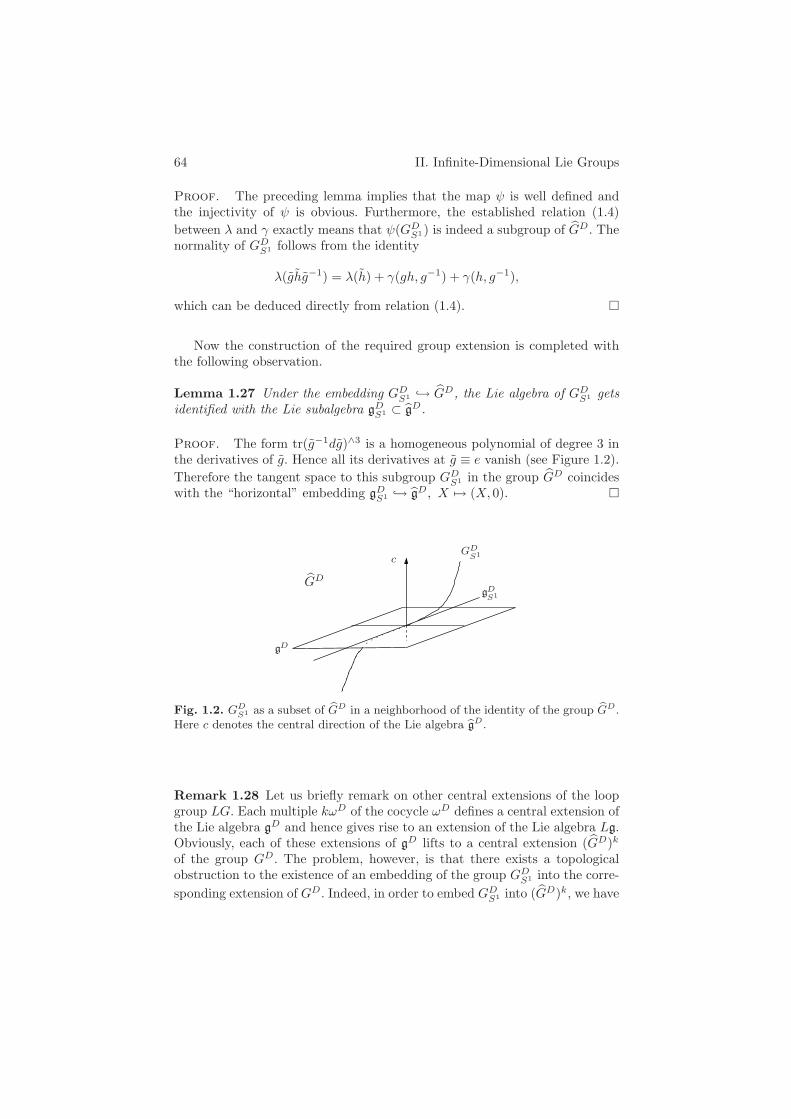
64 II. Infinite-Dimensional Lie Groups
Proof. The preceding lemma implies that the map ψ is well defined andthe injectivity of ψ is obvious. Furthermore, the established relation (1.4)between λ and γ exactly means that ψ(GD
S1) is indeed a subgroup of GD. Thenormality of GD
S1 follows from the identity
λ(ghg−1) = λ(h) + γ(gh, g−1) + γ(h, g−1),
which can be deduced directly from relation (1.4).
Now the construction of the required group extension is completed withthe following observation.
Lemma 1.27 Under the embedding GDS1 → GD, the Lie algebra of GD
S1 getsidentified with the Lie subalgebra gD
S1 ⊂ gD.
Proof. The form tr(g−1dg)∧3 is a homogeneous polynomial of degree 3 inthe derivatives of g. Hence all its derivatives at g ≡ e vanish (see Figure 1.2).Therefore the tangent space to this subgroup GD
S1 in the group GD coincideswith the “horizontal” embedding gD
S1 → gD, X → (X, 0).
gD
gDS1
GDS1
c
GD
Fig. 1.2. GDS1 as a subset of GD in a neighborhood of the identity of the group GD.
Here c denotes the central direction of the Lie algebra gD.
Remark 1.28 Let us briefly remark on other central extensions of the loopgroup LG. Each multiple kωD of the cocycle ωD defines a central extension ofthe Lie algebra gD and hence gives rise to an extension of the Lie algebra Lg.Obviously, each of these extensions of gD lifts to a central extension ( GD)k
of the group GD. The problem, however, is that there exists a topologicalobstruction to the existence of an embedding of the group GD
S1 into the corre-sponding extension of GD. Indeed, in order to embed GD
S1 into ( GD)k, we have

1. Loop Groups and Affine Lie Algebras 65
to use the map g → (g, eikλ(g)). However, Lemma 1.25 shows that the numbereikλ(g) depends on the choice of g unless k is an integer. Hence, we can liftthe central extension of the loop algebra Lg with the cocycle kω to the grouplevel whenever k ∈ Z. It can be shown [322] that these exhaust all possiblecentral extensions of the loop group LG. Moreover, the group extension LGwith k = 1 considered above is singled out among other extensions of the loopgroup LG by the fact that it is simply connected.
1.4 Bibliographical Notes
The standard reference for the material of this section is the by now classicalmonograph by Pressley and Segal [322]. The book [178] describes the theoryof Kac–Moody Lie algebras, while the corresponding groups are treated froman algebraic point of view in [225].
The central extension of the loop algebra goes back to Kac [177] andMoody [275]. The classification of coadjoint orbits of the affine groups wasgiven by Reyman and Semenov-Tian-Shansky [329], Segal [342], and Frenkel[132].
Normal forms of families of matrices up to conjugation are described in[15, 17]. They are related to the description of the coadjoint orbits of nonex-tended loop groups in the GL(n) case. Such families also provide versal defor-mations of the orbits of GL(n)-affine groups in terms of deformations of thecorresponding monodromy operators.
For a finite-dimensional group G that admits an outer automorphism σ offinite order one can define the twisted loop group LGσ = g : R → G | g(θ +2π) = σ(g(θ)) for all θ ∈ R. Central extensions of the twisted loop groups areconstructed in a similar fashion as for the untwisted ones. The correspondingLie algebras are called the twisted affine Lie algebras. The classification of thecoadjoint orbits of the latter algebras is similar to that of the untwisted ones,except that one has to use conjugacy classes of nonconnected compact Liegroups [385].
Irreducible highest-weight representations of affine Lie algebras in both thetwisted and nontwisted cases naturally correspond to, respectively, twistedand standard conjugacy classes in the corresponding compact Lie group [270].In [132] it is shown how the orbit classification for affine groups gives an ana-logue of Kirillov’s character formula for compact Lie groups in the loop groupsetting and relates it to the Wiener integration on the space of continuouspaths in the compact group.
An important class of algebras, related to the affine ones, is given by theKrichever–Novikov-type algebras [219, 220, 336, 353], which we discuss inAppendix A.3. Loop algebras along with their central extensions can be re-garded as subalgebras of the gl∞ algebra (see Appendix A.9), which relatesthem to infinite-dimensional Grassmannians and provides a universal treat-ment of the corresponding soliton equations [75, 176, 372].
66 II. Infinite-Dimensional Lie Groups
The quotient construction of the central extension of the loop group,as described in Section 1.3, has appeared in the physics literature on theWess–Zumino–Witten (or Wess–Zumino–Novikov–Witten) model [263]. Sim-ilar constructions of this group cocycle, its variations, and generalizationscan be found in the papers by Faddeev and Shatashvili [109], Polyakov andWiegmann [319], Witten [387], Mickelsson [262], Pressley and Segal [322],Losev, Moore, Nekrasov, and Shatashvili [241], and others.
Hamiltonian systems related to loop groups and the description of someintegrability mechanisms can be found in [4, 110, 119, 328, 330, 365]; see also[2, 308]. We will touch on certain dynamical systems related to loop groupsin Sections 3 and 5.
Note that systems on loop groups help explain integrability of finite-dimensional discrete systems [77]. The study of Poisson structures ofdifferential-geometric type on loop spaces and the corresponding integrablesystems, initiated by Dubrovin and Novikov in [91, 92], is another directionof active current research; see [272]. It also prompted the theory of Frobeniusmanifolds [89, 251]. Finally, we mention the construction of a universal sym-plectic form for a large class of soliton equations in [221, 218], and the relationbetween integrable Hamiltonian systems and the Riemann–Hilbert problem[76].
For manifolds M of higher dimensions the corresponding current groups,i.e., the spaces of maps from M to a finite-dimensional Lie group G, alongwith their central extensions, are studied in more detail, for example, in [264,322, 248]. We discuss some of these groups in more detail in Section 5, wherewe deal with the case of a two-dimensional manifold M . The case of currentgroups on noncompact manifolds is treated in [288].
2. Diffeomorphisms of the Circle and the Virasoro–Bott Group 67
2 Diffeomorphisms of the Circle and the Virasoro–BottGroup
This section deals with the Lie group Diff(S1) of orientation-preserving diffeo-morphisms of the circle and its Lie algebra Vect(S1) of smooth vector fields onthe circle, as well as with their central extensions. We start by showing thatthe Lie algebra of vector fields on the circle admits a unique nontrivial centralextension, the so-called Virasoro algebra. This central extension gives rise to acentral extension of the Lie group of circle diffeomorphisms, which is called theVirasoro–Bott group. Similar to the case of loop groups, the Virasoro–Bottgroup has a “nicer” coadjoint representation than the nonextended group ofcircle diffeomorphisms. Its coadjoint orbits can be classified in terms of con-jugacy classes of the finite-dimensional group SL(2,R). Finally, we describethe Euler equations corresponding to right-invariant metrics on the Virasoro–Bott group and encounter the KdV and related partial differential equationsamong them.
2.1 Central Extensions
Let us consider the Lie algebra Vect(S1) of smooth vector fields on the circle.After fixing a coordinate θ on the circle, any vector field can be written asf(θ)∂θ, where f is a smooth function on S1 and ∂θ stands for ∂
∂θ . Under thisidentification, the commutator of two elements in Vect(S1) is given by
[f(θ)∂θ, g(θ)∂θ] = (f ′(θ)g(θ) − g′(θ)f(θ))∂θ ,
where f ′ denotes the derivative in θ of the function f .11
Definition / Proposition 2.1 The map ω : Vect(S1)×Vect(S1) → R givenby
ω(f(θ)∂θ, g(θ)∂θ) =∫
S1f ′(θ)g′′(θ)dθ (2.5)
is a nontrivial 2-cocycle on Vect(S1), called the Gelfand–Fuchs cocycle. Thecorresponding central extension of Vect(S1) is called the Virasoro algebra andis denoted by vir.
Exercise 2.2 Prove the cocycle identity for ω.
The following proposition shows that the Virasoro algebra is the unique(up to isomorphism) nontrivial central extension of the Lie algebra Vect(S1).
Proposition 2.3 The second continuous cohomology group H2(Vect(S1),R)is one-dimensional and is generated by the Gelfand–Fuchs cocycle ω.11 Note that this Lie bracket is the negative of the commonly assumed commutator
of vector fields, as the calculations in Exercise 2.3 of Chapter I shows; see [24].
68 II. Infinite-Dimensional Lie Groups
Proof. The proof of this proposition (see [322]) is similar to that ofProposition 1.6. Our goal is to show that, up to a coboundary, any continuous2-cocycle ω on the Lie algebra Vect(S1) is a multiple of the Gelfand–Fuchscocycle. First, let us extend the cocycle ω from Vect(S1) to a complex bilin-ear form on the complexification Vect(S1)C = Vect(S1)⊗C of the Lie algebraVect(S1). An element f(θ)∂θ ∈ Vect(S1)C can be expanded into a Fourierseries
f(θ) =∑
fneinθ .
By continuity, the cocycle ω is completely determined by its values on thebasis fields Ln = ieinθ∂θ. Note that the commutator of the fields Ln and Lm
is given by[Ln, Lm] = (m− n)Ln+m .
The cocycle identity for ω and the triple L0, Lm, Ln gives
ω([L0, Lm], Ln) + ω(Lm, [L0, Ln]) = ω(L0, [Lm, Ln]) ,
which implies that the cohomology class of the cocycle ω is unchanged underrotations of S1 that are generated by the vector field L0. Indeed, the right-hand side of the equation above is an exact cocycle (i.e., coboundary) dα,where α is the linear functional on Vect(S1) defined by α(Lm) := ω(L0, Lm).(Here by definition dα(Ln, Lm) := α([Ln, Lm]).) In particular, the cocycleobtained from ω by averaging over S1 belongs to the same cohomology classas ω. Therefore, we can assume ω to be rotation invariant, i.e.,
ω([L0, Lm], Ln) + ω(Lm, [L0, Ln]) = 0 . (2.6)
Set ωn,m := ω(Ln, Lm). Then the commutator relation of the fields Ln
and Lm and equation (2.6) imply
mωm,n + nωm,n = 0 .
This implies that ωm,n = 0 for m + n = 0. Antisymmetry of the cocycle ωimplies ωn,−n = ω−n,n, so that it is enough to determine ωn,−n for n ∈ N.
The cocycle identity for ω evaluated on the triple Lm, Ln, L−m−n implies
(m− n)ωm+n,−n−m + (2m+ n)ωn,−n − (2n+m)ωm,−m = 0 .
In particular, for m = 1 the equation above reads as follows:
(−n+ 1)ωn+1,−n−1 + (n+ 2)ωn,−n − (2n+ 1)ω1,−1 = 0 .
Hence ωn,−n is defined recursively once ω1,−1 and ω2,−2 are fixed. This showsthat the space of the bilinear forms ω that satisfy the 2-cocycle condition isat most two-dimensional. Two linear independent elements of this space aregiven by ωn,−n = n3 and ωn,−n = n. But the 2-cocycle defined by ωn,−n = n
2. Diffeomorphisms of the Circle and the Virasoro–Bott Group 69
is exact, since it coincides with dα, where α is the linear functional definedby α(Ln) = − 1
2δn,0.So up to a 2-coboundary, any 2-cocycle ω has the “cubic” form
ω(Ln, Lm) = cδn,−mn3
for some c ∈ C.It remains to show that the “cubic” cocycle ω is nontrivial. Suppose
that ω = dβ for some 1-cocycle β. This means that β is a linear map andω(Ln, Lm) = β([Ln, Lm]). In particular, we have β([Ln, L−n]) = 2niβ(L0),which shows that in this case ω(Ln, L−n) would have to depend linearly on n.This contradiction completes the proof.
Our next goal is to show that the central extension of the Lie algebra ofvector fields Vect(S1) defined by the Gelfand–Fuchs cocycle ω can be lifted toa central extension of the group of circle diffeomorphisms Diff(S1). It turnsout that the situation here is much simpler than that in the case of the loopgroups. The central extension of the group Diff(S1) corresponding to the Liealgebra vir is topologically trivial and hence can be defined by a continuousgroup 2-cocycle.
Let ϕ : θ → ϕ(θ) be a diffeomorphism of the circle, and ϕ′ stands for itsderivative in θ.
Definition / Proposition 2.4 The map B : Diff(S1)×Diff(S1) → S1 givenby
(ϕ,ψ) → 12
∫
S1log(ϕ ψ)′d logψ′
is a continuous 2-cocycle on the group Diff(S1). The Lie algebra of the corre-sponding central extension Diff(S1) is the Virasoro algebra vir. The 2-cocycleB is called the Bott cocycle, and the corresponding central extension of thegroup Diff(S1) is called the Virasoro–Bott group.
Proof. To show that the map B defines a group 2-cocycle, we have to checkthe identity
B(ϕ ψ, η) +B(ϕ,ψ) = B(ϕ,ψ η) +B(ψ, η) .
It is provided by the chain rule, which immediately gives
B(ϕψ, η) =12
∫
S1log(ϕψη)′ d log η′ =
12
∫
S1log(ϕ′ψη) d log η′+B(ψ, η)
and
70 II. Infinite-Dimensional Lie Groups
B(ϕ,ψ η) =12
∫
S1log(ϕ ψ η)′ d log(ψ η)′
= B(ϕ,ψ) +12
∫
S1log(ϕ′ ψ η) d log η′ .
Now we verify that the infinitesimal version of the Bott group cocycle Bcoincides with the Gelfand–Fuchs Lie algebra 2-cocycle ω. Let f∂θ and g∂θ betwo smooth vector fields on S1 and consider the corresponding flows ϕs andψt on S1, starting at the identity diffeomorphism: ϕ0 = ψ0 = id.
We have to check that
ω(f∂θ, g∂θ) =d2
dt ds
∣
∣
∣
t=0,s=0B(ϕt, ψs) −
d2
dt ds
∣
∣
∣
t=0,s=0B(ψs, ϕt)
(see Proposition 3.14 of Chapter I). The latter holds, since
d
dt
∣
∣
∣
t=0B(ϕt, ψs) =
12
∫
S1
(
log′(ϕ0 ψs)′)
(f ψs)′d logψ′s
=12
∫
S1(f ′ ψs) d logψ′
s
andd
ds
∣
∣
∣
s=0
12
∫
S1(f ′ ψs) d logψ′
s =12
∫
S1f ′dg′ .
Similarly, we obtain
d2
dt ds
∣
∣
∣
t=0,s=0B(ψs, ϕt) =
12
∫
S1g′df ′ = −1
2
∫
S1f ′dg′ ,
which, combined with the equation above, yields the assertion.
2.2 Coadjoint Orbits of the Group of Circle Diffeomorphisms
Before we start classifying the coadjoint orbits of the Virasoro group, letus take a look at the coadjoint representation of the nonextended group oforientation-preserving diffeomorphisms of the circle. Observe that the dualspaces to the infinite-dimensional Lie algebras considered below are alwaysunderstood as smooth duals, i.e., they are identified with appropriate spacesof smooth functions.
Let Diff(S1) be the group of all orientation-preserving diffeomorphisms ofS1 and let Vect(S1) be its Lie algebra.
Proposition 2.5 ([202]) The (smooth) dual space Vect(S1)∗ is naturallyidentified with the space of quadratic differentials Ω⊗2(S1) = u(θ)(dθ)2 onthe circle. The pairing is given by the formula

2. Diffeomorphisms of the Circle and the Virasoro–Bott Group 71
〈u(θ)(dθ)2, v(θ)∂θ)〉 =∫
S1u(θ)v(θ) dθ
for any vector field v(θ)∂θ ∈ Vect(S1). The coadjoint action coincides with theaction of a diffeomorphism on the quadratic differential: for a diffeomorphismϕ ∈ Diff(S1) the action is
Ad∗ϕ−1 : u (dθ)2 → u(ϕ) · (ϕ′)2 (dθ)2 = u(ϕ) · (dϕ)2.
It follows from this proposition that the square root√
u(θ)(dθ)2 (whenit makes sense) transforms under a diffeomorphism as a differential 1-form.In particular, if the function u(θ) does not have any zeros on the circle (say,u(θ) > 0), then Φ(u(θ)(dθ)2) :=
∫
S1
√
u(θ) dθ is a Casimir function, i.e., aninvariant of the coadjoint action. One can see that there is only one Casimirfunction in this case, since the corresponding orbit has codimension 1 in thedual space Vect(S1)∗. Indeed, there exists a diffeomorphism that sends thequadratic differential u(θ)(dθ)2 without zeros to the constant quadratic dif-ferential u0(dθ)2, where the constant u0 is such that
√u0 is the average value
of the 1-form√
u(θ) dθ on the circle:
2π√u0 =
∫
S1
√
u(θ) dθ .
The value u0 parametrizes the orbits close to u(θ)(dθ)2, and hence all these or-bits have codimension 1 in Ω⊗2(S1). The stabilizer of a constant quadratic dif-ferential is the group S1 of rigid rotations, so that the orbit through u(θ)(dθ)2
is diffeomorphic to Diff(S1)/S1.On the other hand, if a differential u(θ)(dθ)2 changes sign on the circle,
then the integrals∫ b
a
√
|u(θ)| dθ ,
evaluated between any two consecutive zeros a and b of the function u(θ), areinvariant. In particular, since u(θ) has at least two zeros, the coadjoint orbitof such a differential u(θ)(dθ)2 necessarily has codimension higher than 1,and there exist coadjoint orbits of the group Diff(S1) of arbitrarily highcodimension. The classification of orbits in Vect(S1)∗ was described in[201, 203].
Remark 2.6 One can show that if the function u(θ) has two simple zeros,changing sign exactly twice on the circle, then the corresponding coadjointorbit of the group Diff(S1) has codimension 2; see [203]. (The correspond-ing two Casimirs are the integrals of
√
|u(θ)| dθ over two different parts ofthe circle between these two zeros, while there are no extra local invariantsat zeros themselves: quadratic differentials with simple zeros are all locallydiffeomorphic to ±θ (dθ)2.)

72 II. Infinite-Dimensional Lie Groups
In other words, in a family of quadratic differentials uε := uε(θ) (dθ)2,where the function uε is everywhere positive for ε > 0, has a double zerofor ε = 0, and has two simple zeros for ε < 0 (e.g., uε = cos θ + 1 + ε) thecodimension of the coadjoint orbit of uε = uε(dθ)2 changes from 1 for ε > 0to 2 for ε ≤ 0, since the number of Casimirs jumps from 1 to 2. (Note thatfor ε = 0 the orbit codimension of u0 is also 2, since the existence of a doublezero imposes an extra constraint on a quadratic differential.)
This change of “codimension parity” of the (infinite-dimensional) coad-joint orbits is rather surprising, since in finite dimensions the existence of asymplectic structure on each coadjoint orbit forces all of them to be even-dimensional, and hence codimensions of coadjoint orbits for a given (finite-dimensional) group are always of the same parity: either all even or all odd.However, for Vect(S1)∗ = Ω⊗2(S1) we observe that there exist orbits of bothcodimensions 1 and 2!
In particular, this shows that the Weinstein theorem [384] on the exis-tence of the transverse Poisson structure to symplectic leaves does not holdfor infinite-dimensional Poisson manifolds; cf. Remark I.4.7. Indeed, on a two-dimensional transversal to u0 in Vect(S1)∗, neighboring coadjoint orbits of uε
have traces of both codimensions 1 and 2. One can consider the following ex-ample, clarifying how the change of parity can occur for infinite-dimensionalsymplectic leaves. Define the Poisson structure in an infinite-dimensional vec-tor space (x0, x1, x2, . . . ) by the bivector field
Π = x0 ∂x1 ∧ ∂x2 + ∂x2 ∧ ∂x3 + ∂x3 ∧ ∂x4 + . . . .
Its symplectic leaves are hyperplanes x0 = const = 0, while for x0 = 0 thesymplectic leaves are planes x0 = 0, x1 = const of codimension 2.
In the next section, however, we shall see that coadjoint orbits of theVirasoro group, the central extension of the diffeomorphism group Diff(S1), dorespect the codimension parity and behave much more like finite-dimensionalcoadjoint orbits.
2.3 The Virasoro Coadjoint Action and Hill’s Operators
Let vir be the Virasoro algebra, whose elements are pairs (f(θ)∂θ, c), wheref(θ)∂θ is a vector field and c is a real number. We can think of its (smooth)dual space as the space of pairs vir
∗ = (u(θ)(dθ)2, a) consisting of aquadratic differential and a real number (the cocentral term). The pairingbetween vir and vir
∗ is given by
〈(f(θ)∂θ, c), (u(θ)(dθ)2, a)〉 =∫
S1f(θ)u(θ)dθ + c · a .
Our goal in this section is to derive a classification of the coadjoint orbitsof the Virasoro–Bott group Diff(S1). This classification turns out to be similar
2. Diffeomorphisms of the Circle and the Virasoro–Bott Group 73
to that of the coadjoint orbits of the centrally extended loop groups inSection 1.2.
We begin by noticing that the center of the group Diff(S1) acts triviallyon the dual space vir
∗. This is why to describe the coadjoint representation ofthe Virasoro–Bott group we need the action of (nonextended) diffeomorphismsonly.
Definition / Proposition 2.7 The coadjoint action of a diffeomorphismϕ ∈ Diff(S1) on the dual vir
∗ of the Virasoro algebra is given by the followingformula:
Ad∗ϕ−1 : (u (dθ)2, a) →
(
u(ϕ) · (ϕ′)2 (dθ)2 + aS(ϕ) (dθ)2, a)
, (2.7)
where
S(ϕ) =ϕ′ϕ′′′ − 3
2 (ϕ′′)2
(ϕ′)2
is the Schwarzian derivative of the diffeomorphism ϕ.
The same formula can be used to define the Schwarzian derivative S(φ)for a smooth map φ : R → R or R → RP 1 S1.
Proof. The coadjoint action of the Virasoro algebra is defined by theidentity
〈ad∗(v∂θ,b)(u(dθ)2, a), (w∂θ, c)〉 = −〈(u(dθ)2, a), [(v∂θ, b), (w∂θ, c)]〉.
Using the definition of the Virasoro commutator and integrating by parts weobtain that the right-hand side is equal to
∫
S1−w(2uv′ + u′v + av′′′) dθ .
Thus the coadjoint operator is
ad∗(v∂θ,b)(u(dθ)2, a) = −((2uv′ + u′v + av′′′)(dθ)2, 0). (2.8)
It remains to check that equation (2.7) indeed defines a representation ofthe group Diff(S1) on the space vir
∗ and that the infinitesimal version of thisaction is given by equation (2.8). Both assertions can be checked by directcalculations, which we leave to the reader.
Exercise 2.8 Prove the following transformation law for the Schwarzianderivative:
S(ϕ ψ) = (S(ϕ) ψ) · (ψ′)2 + S(ψ) . (2.9)
Check that the formula (2.7) defines a group representation by using this law.

74 II. Infinite-Dimensional Lie Groups
It turns out to be more convenient to regard the dual Virasoro space vir∗
not as the space of pairs (u(θ)(dθ)2, a), but as the space of Hill’s operators,i.e., differential operators a∂2
θ +u(θ), where ∂2θ stands for the second derivative
d2/dθ2. Indeed, the group action on Hill’s operators
Ad∗ϕ−1 : a∂2
θ + u(θ) → a∂2θ + u(ϕ) · (ϕ′)2 + aS(ϕ) (2.10)
has the following nice geometric interpretation (see, e.g., [342, 202, 205, 304]).Look at a hyperplane a = const corresponding to nonzero a in the dual
space vir∗. For instance, we fix a = 1 and consider Hill’s operators of the form
∂2θ + u(θ), where θ is a coordinate on S1. Let f and g be two independent
solutions of the corresponding Hill differential equation
(∂2θ + u(θ))y = 0 (2.11)
for an unknown function y. Although this equation has periodic coefficients,the solutions need not necessarily be periodic, but instead are defined over R.Consider the ratio η := f/g : R → RP 1. (Below we use the same notation θfor the coordinate on the circle S1 = R/2πZ and on its cover R.)
Proposition 2.9 The potential u is (one-half) the Schwarzian derivative ofthe ratio η:
u =S(η)
2.
Proof. First we note that the Wronskian
W (f, g) := det(
f gf ′ g′
)
= fg′ − f ′g
is constant, since it satisfies W ′ = 0. For two independent solutions theWronskian does not vanish, and we normalize W by setting W = −1.
This additional condition allows one to find the potential u from theratio η. Indeed, first one reconstructs the solutions f and g from the ratioη by differentiating:
η′ =f ′g − fg′
g2=
−Wg2
=1g2
.
Therefore,
g =1√η′, f = g · η =
η√η′.
Given two solutions f and g, one immediately finds the corresponding differ-ential equation they satisfy by writing out the following 3 × 3 determinant:
det
⎡
⎣
y f gy′ f ′ g′
y′′ f ′′ g′′
⎤
⎦ = 0 .
2. Diffeomorphisms of the Circle and the Virasoro–Bott Group 75
Since f and g satisfy the equation y′′ + u · y = 0, one obtains from thedeterminant above that
u = −det[
f ′ g′
f ′′ g′′
]
.
The explicit formula for u expressed in terms of η turns out to be one-half theSchwarzian derivative of η.
Corollary 2.10 The Schwarzian derivative S(η) is invariant with respect toa Mobius transformation η → (aη+b)/(cη+d), where a, b, c, d are real numberssuch that ad− bc = 1.
In particular, if η itself is a Mobius transformation η : θ → (aθ+b)/(cθ+d),then S(η) = S(id) = 0, where id : θ → θ.
Proof. Indeed, for a given potential u the solutions f and g of the corre-sponding differential equation are not defined uniquely, but up to a transfor-mation of the pair (f, g) by a matrix from SL(2,R). Then the ratio η changesby a Mobius transformation. Thus Mobius equivalent ratios η correspond tothe same potential u = S(η)/2. For the identity diffeomorphism id : θ → θ,the explicit formula for the Schwarzian derivative gives S(id) = 0.
Proposition 2.11 The Virasoro coadjoint action of a diffeomorphism ϕ onthe potential u(θ) gives rise to a diffeomorphism change of coordinate in theratio η:
ϕ : η(θ) → η(ϕ(θ)) .
Proof. We look at the corresponding infinitesimal action on the solutionsof the differential equation (∂2
θ + u(θ))y = 0. For a diffeomorphism ϕ−1(θ) =θ + εv(θ) close to the identity, consider the infinitesimal Virasoro action ofϕ−1 on the potential u(θ):
u → u+ ε · δu, where δu = 2uv′ + u′v +12v′′′
(cf. formula (2.8) for a = 12 and note that we are considering the action of
ϕ−1). It is consistent with the following action on a solution y of the abovedifferential equation:
y → y + ε · δy, where δy = −12yv′ + y′v.
The consistency means that (∂2θ + u+ ε · δu)(y + ε · δy) = 0 + O(ε2).
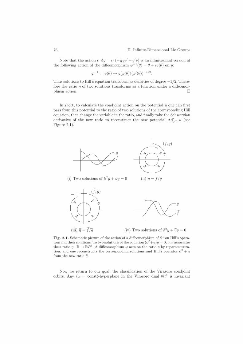
76 II. Infinite-Dimensional Lie Groups
Note that the action ε · δy = ε · (− 12yv
′ + y′v) is an infinitesimal version ofthe following action of the diffeomorphism ϕ−1(θ) = θ + εv(θ) on y:
ϕ−1 : y(θ) → y(ϕ(θ))(ϕ′(θ))−1/2.
Thus solutions to Hill’s equation transform as densities of degree −1/2. There-fore the ratio η of two solutions transforms as a function under a diffeomor-phism action.
In short, to calculate the coadjoint action on the potential u one can firstpass from this potential to the ratio of two solutions of the corresponding Hillequation, then change the variable in the ratio, and finally take the Schwarzianderivative of the new ratio to reconstruct the new potential Ad∗
ϕ−1u (seeFigure 2.1).
˜f
g
( ˜f, g)
(f, g)
(i) Two solutions of ∂2y + uy = 0 (ii) η = f/g
(iii) η = ˜f/g
fg
(iv) Two solutions of ∂2y + uy = 0
Fig. 2.1. Schematic picture of the action of a diffeomorphism of S1 on Hill’s opera-tors and their solutions: To two solutions of the equation (∂2+u)y = 0, one associatestheir ratio η : R → RP 1. A diffeomorphism ϕ acts on the ratio η by reparametriza-tion, and one reconstructs the corresponding solutions and Hill’s operator ∂2 + ufrom the new ratio η.
Now we return to our goal, the classification of the Virasoro coadjointorbits. Any (a = const)-hyperplane in the Virasoro dual vir
∗ is invariant
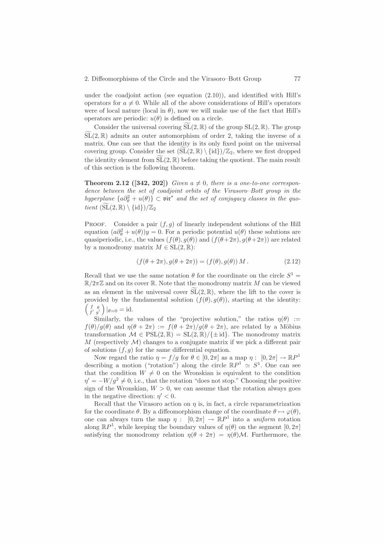
2. Diffeomorphisms of the Circle and the Virasoro–Bott Group 77
under the coadjoint action (see equation (2.10)), and identified with Hill’soperators for a = 0. While all of the above considerations of Hill’s operatorswere of local nature (local in θ), now we will make use of the fact that Hill’soperators are periodic: u(θ) is defined on a circle.
Consider the universal covering ˜SL(2,R) of the group SL(2,R). The group˜SL(2,R) admits an outer automorphism of order 2, taking the inverse of amatrix. One can see that the identity is its only fixed point on the universalcovering group. Consider the set (˜SL(2,R) \ id)/Z2, where we first droppedthe identity element from ˜SL(2,R) before taking the quotient. The main resultof this section is the following theorem.
Theorem 2.12 ([342, 202]) Given a = 0, there is a one-to-one correspon-dence between the set of coadjoint orbits of the Virasoro–Bott group in thehyperplane a∂2
θ + u(θ) ⊂ vir∗ and the set of conjugacy classes in the quo-
tient (˜SL(2,R) \ id)/Z2
Proof. Consider a pair (f, g) of linearly independent solutions of the Hillequation (a∂2
θ + u(θ))y = 0. For a periodic potential u(θ) these solutions arequasiperiodic, i.e., the values (f(θ), g(θ)) and (f(θ+2π), g(θ+2π)) are relatedby a monodromy matrix M ∈ SL(2,R):
(f(θ + 2π), g(θ + 2π)) = (f(θ), g(θ))M . (2.12)
Recall that we use the same notation θ for the coordinate on the circle S1 =R/2πZ and on its cover R. Note that the monodromy matrix M can be viewedas an element in the universal cover ˜SL(2,R), where the lift to the cover isprovided by the fundamental solution (f(θ), g(θ)), starting at the identity:(
f gf ′ g′
)
|θ=0 = id.Similarly, the values of the “projective solution,” the ratios η(θ) :=
f(θ)/g(θ) and η(θ + 2π) := f(θ + 2π)/g(θ + 2π), are related by a Mobiustransformation M ∈ PSL(2,R) = SL(2,R)/± id. The monodromy matrixM (respectively M) changes to a conjugate matrix if we pick a different pairof solutions (f, g) for the same differential equation.
Now regard the ratio η = f/g for θ ∈ [0, 2π] as a map η : [0, 2π] → RP 1
describing a motion (“rotation”) along the circle RP 1 S1. One can seethat the condition W = 0 on the Wronskian is equivalent to the conditionη′ = −W/g2 = 0, i.e., that the rotation “does not stop.” Choosing the positivesign of the Wronskian, W > 0, we can assume that the rotation always goesin the negative direction: η′ < 0.
Recall that the Virasoro action on η is, in fact, a circle reparametrizationfor the coordinate θ. By a diffeomorphism change of the coordinate θ → ϕ(θ),one can always turn the map η : [0, 2π] → RP 1 into a uniform rotationalong RP 1, while keeping the boundary values of η(θ) on the segment [0, 2π]satisfying the monodromy relation η(θ + 2π) = η(θ)M. Furthermore, the

78 II. Infinite-Dimensional Lie Groups
number of rotations (the “winding number”) for the map η : [0, 2π] → RP 1
does not change under a reparametrization by a circle diffeomorphism ϕ.In other words, the orbits of the maps η (or, equivalently, of the potentialsu(x)) are described by one continuous parameter (the conjugacy class ofM) and one discrete parameter (the winding number). One can see that thesetwo parameters together encode nothing else but the conjugacy class of themonodromy matrices M in the universal covering of SL(2,R).
Note that the choice in the sign of the Wronskian reflects the Z2-actionon the universal covering ˜SL(2,R). Indeed, with this choice (W > 0) the pathη always goes in the negative direction (η′ < 0), so one can reach only the“negative half” of the conjugacy classes in the universal cover ˜SL(2,R).
Finally, note that the identity matrix in the universal covering ˜SL(2,R)(or in its projectivization ˜SL(2,R)/Z2) cannot be obtained as a monodromymatrix for the maps η : [0, 2π] → RP 1. Indeed, any map η starting at theidentity has to move out from it, since η′(0) = 0.
Corollary 2.13 The Virasoro orbits in the hyperplane a∂2θ + u(θ) | a =
a0 ⊂ vir∗ with fixed a0 = 0 are classified by the Jordan normal form of
matrices in SL(2,R) and by a positive integer parameter, the winding num-ber. In this hyperplane a = a0 of the dual vir
∗ the orbit containing Hill’soperator a∂2
θ + u(θ) has codimension equal to the codimension in SL(2,R) ofthe conjugacy class of the monodromy matrix M corresponding to this Hill’soperator.
Matrices in the group SL(2,R) split into three classes, whose normal formsare the exponentials of the following three classes in the Lie algebra sl(2,C),the complexification of sl(2,R):
(i)(
µ 00 −µ
)
, (ii)(
0 ±10 0
)
, and (iii)(
0 00 0
)
; (2.13)
see Figure 2.2. The codimensions of the corresponding conjugacy classes inSL(2,R) are 1 in cases (i) and (ii), and 3 in case (iii). Note that the set of realmatrices that are exponentials of (i)-type matrices consists of the elliptic andhyperbolic parts: rotation matrices (for µ ∈ iR) and hyperbolic rotations (forµ ∈ R). Furthermore, hyperbolic rotations correspond to one-sheeted hyper-boloids. Rotations in the clockwise and counterclockwise directions correspondto different sheets of two-sheeted hyperboloids, and they belong to differentconjugacy classes in SL(2,R). (The rotation by 180 has a three-dimensionalstabilizer and corresponds to a one-point conjugacy class.) The group SL(2,R)is topologically a solid torus, and the adjacency of conjugacy classes describedin Figure 2.2 is observed near both id and − id in this group.
The equality of the codimensions of the Virasoro coadjoint orbits invir
∗ and the codimensions of (the conjugacy classes of) the corresponding
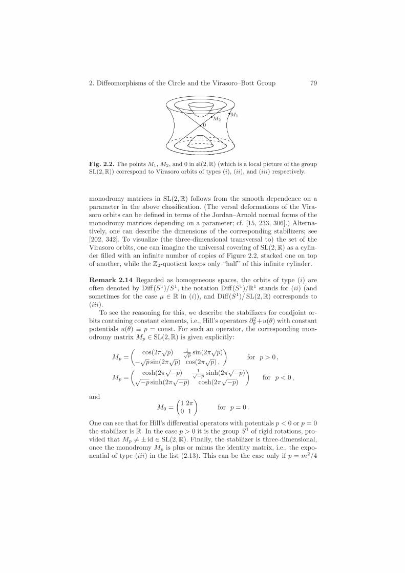
2. Diffeomorphisms of the Circle and the Virasoro–Bott Group 79
0
M1M2
Fig. 2.2. The points M1, M2, and 0 in sl(2, R) (which is a local picture of the groupSL(2, R)) correspond to Virasoro orbits of types (i), (ii), and (iii) respectively.
monodromy matrices in SL(2,R) follows from the smooth dependence on aparameter in the above classification. (The versal deformations of the Vira-soro orbits can be defined in terms of the Jordan–Arnold normal forms of themonodromy matrices depending on a parameter; cf. [15, 233, 306].) Alterna-tively, one can describe the dimensions of the corresponding stabilizers; see[202, 342]. To visualize (the three-dimensional transversal to) the set of theVirasoro orbits, one can imagine the universal covering of SL(2,R) as a cylin-der filled with an infinite number of copies of Figure 2.2, stacked one on topof another, while the Z2-quotient keeps only “half” of this infinite cylinder.
Remark 2.14 Regarded as homogeneous spaces, the orbits of type (i) areoften denoted by Diff(S1)/S1, the notation Diff(S1)/R1 stands for (ii) (andsometimes for the case µ ∈ R in (i)), and Diff(S1)/SL(2,R) corresponds to(iii).
To see the reasoning for this, we describe the stabilizers for coadjoint or-bits containing constant elements, i.e., Hill’s operators ∂2
θ +u(θ) with constantpotentials u(θ) ≡ p = const. For such an operator, the corresponding mon-odromy matrix Mp ∈ SL(2,R) is given explicitly:
Mp =(
cos(2π√p) 1√
p sin(2π√p)
−√p sin(2π
√p) cos(2π
√p) ,
)
for p > 0 ,
Mp =(
cosh(2π√−p) 1√−p
sinh(2π√−p)√−p sinh(2π
√−p) cosh(2π√−p)
)
for p < 0 ,
and
M0 =(
1 2π0 1
)
for p = 0 .
One can see that for Hill’s differential operators with potentials p < 0 or p = 0the stabilizer is R. In the case p > 0 it is the group S1 of rigid rotations, pro-vided that Mp = ± id ∈ SL(2,R). Finally, the stabilizer is three-dimensional,once the monodromy Mp is plus or minus the identity matrix, i.e., the expo-nential of type (iii) in the list (2.13). This can be the case only if p = m2/4
80 II. Infinite-Dimensional Lie Groups
for some m ∈ N. In the latter case, the stabilizer of the corresponding Hill’sequation is the m-fold covering of PSL(2,R) in Diff(S1).
Finally, we note that the trace function tr : SL(2,R) → R is invariant onconjugacy classes in SL(2,R) and it gives rise to a Casimir function on thehyperplane a = a0 ⊂ vir
∗ for the Lie–Poisson bracket: tra0∂2θ + u(θ) :=
tr(M), where M is a monodromy matrix of the given Hill operator. Alongwith the value of a, this is the only Casimir for generic Virasoro orbits, sincetheir codimension in the hyperplane a = a0 is equal to 1.
2.4 The Virasoro–Bott Group and the Korteweg–de VriesEquation
The Korteweg–de Vries (or KdV) equation is the nonlinear evolution equation
ut = −3uu′ − au′′′ , (2.14)
which describes traveling waves in a shallow canal. Here, u is a function of thetime variable t and one space variable θ, ut and u′ denote the correspondingpartial derivatives in t and θ, and a is a nonzero constant. A brief history ofthis equation can be found in [294].
In this section we show how the Korteweg–de Vries equation appears asthe Euler equation with respect to a certain right-invariant metric on theVirasoro–Bott group. Recall that the Euler equation with respect to a right-invariant metric on a Lie group G is a dynamical system on the correspondingLie algebra g describing the evolution of the tangent vector along a geodesic onG, where this vector is pulled back to the Lie algebra of G by right translation;see Section I.4.
Consider the L2-inner product on the Virasoro algebra vir = Vect(S1)⊕R
defined by
〈(v(θ)∂θ, a), (w(θ)∂θ, c)〉 =∫
S1v(θ)w(θ)dθ + a · c . (2.15)
Extend this quadratic form to every tangent space on the Virasoro–Bott groupby right translations to define a (weak) right-invariant L2-metric on the group.
Theorem 2.15 ([305]) The Euler equation for the right-invariant L2-metricon the Virasoro group is (the family of) the KdV equation:
ut = −3uu′ − au′′′ , (2.16)at = 0 . (2.17)
Proof. According to Arnold’s Theorem I.4.14, the Euler equation on g∗ forthe right-invariant metric on the group G has the form

2. Diffeomorphisms of the Circle and the Virasoro–Bott Group 81
d
dtm(t) = ad∗
A−1m(t) m(t) , (2.18)
where m(t) is a point in g∗, and A : g → g∗ is the inertia operator defined bythe metric (using the left-invariant metric would give the minus sign in theequation; cf. Remark I.4.16).
In the Virasoro coadjoint action, an element (v∂θ, c) ∈ vir of the Virasoroalgebra acts on an element (u(dθ)2, a) ∈ vir
∗ of the dual space via
ad∗(v∂θ,c)(u(dθ)2, a) = ((−2v′u− vu′ − av′′′)(dθ)2, 0) ;
see equation (2.8). Furthermore, the L2-inner product gives rise to the “iden-tity” inertia operator A : vir → vir
∗:
(u∂θ, a) → (u(dθ)2, a) ,
mapping a vector field u(θ)∂θ to the quadratic differential u(θ)(dθ)2 with thesame function u(θ).
Then, substituting (u(dθ)2, a) for m, we see that the Euler equation (2.18)becomes
d
dt(u(dθ)2, a) = ((−3uu′ − au′′′)(dθ)2, 0) ,
from which one immediately reads off the KdV equation (2.16), (2.17).
The component a does not change with time (see equation (2.17))and playsthe role of a constant parameter in the KdV equation. It has the physicalmeaning of the characteristic thickness of the shallow-water approximation(see, e.g., [228], p. 169).
Remark 2.16 One can study more general metrics on the Virasoro algebra,some of which are of particular interest in mathematical physics. Consider, forinstance, the following two-parameter family of weighted H1
α,β-inner productson vir:
〈(v∂θ, b), (w∂θ, c)〉H1α,β
=∫
S1(α vw + β v′w′) dθ + bc .
The case α = 1, β = 0 corresponds to the L2 inner product above, whileα = β = 1 corresponds to the H1 product.
Theorem 2.17 ([192]) The Euler equations for the right-invariant H1α,β-
metric (with α = 0) on the Virasoro group are given by the following system:
α(ut + 3uu′) − β((u′′)t + 2u′u′′ + uu′′′) + au′′′ = 0 , (2.19)at = 0 . (2.20)

82 II. Infinite-Dimensional Lie Groups
Exercise 2.18 Give a proof of the latter theorem along the lines of the proofof the L2-case above. (Hint: The inertia operator for the weighted H1 metricis
A : (v∂θ, a) → ((Λv)(dθ)2, a),
where Λ := α − β∂2θ is a second-order differential operator. Verify that in
terms of v = Λ−1u the Euler equation has the form
d
dt(Λv) = −2(Λv)v′ − (Λv′)v + av′′′ ,
which is equivalent to equation (2.19).)
Remark 2.19 For α = 1, β = 0, equation (2.19) is the KdV equation (2.16).For α = β = 1, one recovers the Camassa–Holm equation (see [268]). Forα = 0, β = 1, equation (2.19) becomes the Hunter–Saxton equation. We notethat in the case of α = 0, the H1
α,β-metric becomes the homogeneous H1-metric, which is degenerate. Therefore, to define the Euler equations one hasto pass to the homogeneous space Diff(S1)/S1 (or Diff(S1)/S1) and define thegeodesic flow on it; see details in [192]. It turns out that the space Diff(S1)/S1
equipped with the H1-metric is isometric to an open subset of an L2-sphere;see [237, 238]. This isometry, in particular, allows one to extend solutions ofthe Hunter–Saxton equation beyond breaking time and interpret them afterwave-breaking in an appropriate weak sense.
We also note that the case a = 0 corresponds to the nonextended Liealgebra Vect(S1) of vector fields on the circle, rather than to the Virasoroalgebra vir. In the nonextended case, depending on the values of α and β,one obtains the Hopf (or inviscid Burgers) equation ut + 3uu′ = 0 or thenonextended Camassa–Holm equation [69, 127]
ut + 3uu′ + 2u′u′′ + uu′′′ + (u′′)t = 0 .
2.5 The Bi-Hamiltonian Structure of the KdV Equation
The KdV equation is not only a Hamiltonian system; it also exhibits strongintegrability properties. As we discussed before, there are various definitionsof what an integrable infinite-dimensional system is: one can require fromthe system either the existence of action-angle coordinates, or the existence of“sufficiently many” independent integrals of motion, or some other properties,which may differ substantially in infinite dimensions. In this section we showthat the KdV equation is not only Hamiltonian, but in fact bi-Hamiltonian,thus exhibiting one of the “strongest forms” of integrability. More precisely,in addition to being Hamiltonian with respect to the Lie–Poisson bracket onthe dual space vir
∗, this equation turns out to be Hamiltonian with respectto another compatible Poisson structure on the same space.
Recall that for any Lie algebra g, every point m0 ∈ g∗ gives rise to a“constant” Poisson bracket , 0 on g∗ by “freezing” the usual Lie–Poisson

2. Diffeomorphisms of the Circle and the Virasoro–Bott Group 83
bracket , LP at the point m0. The constant Poisson bracket is defined forsmooth functions f, g on g∗ by
f, g0(m) := 〈[dfm, dgm],m0〉 ;
see Section I.4.4. Furthermore, the Poisson brackets , LP and , 0 arecompatible for all choices of the point m0 (see Lemma I.4.21). The main goalof this section is to show that for a certain choice of the “freezing point”m0 ∈ vir
∗, the KdV equation is Hamiltonian with respect to the constantPoisson structure , 0. Note that other equations discussed above (Camassa–Holm, Hunter–Saxton) have a similar bi-Hamiltonian structure, but relatedto different choices of the “freezing point”; see [192].
Theorem 2.20 The KdV equation (2.14) is Hamiltonian with respect to theconstant Poisson bracket on vir
∗ with the “freezing point” m0 = (12 (dθ)2, 0) ∈
vir∗.
Proof. Let F (u, a) be a function on vir∗ and let (v∂θ, b) :=
(δF/δu, δF/δa) ∈ vir be the (variational) derivative dF(u(dθ)2,a) of F at(u(dθ)2, a). Then the Hamiltonian equation with the Hamiltonian functionF , computed with respect to the constant Poisson structure “frozen” at(u0(dx)2, a0), has the form
d
dt(u(dθ)2, a) = ad∗
(v∂θ,b)(u0(dθ)2, a0) = −(
(2u0v′ + (u0)′v + a0v
′′′)(dθ)2, 0)
.
(Here we use Remark I.4.22 and the explicit form (2.8) of the coadjoint actionad∗ for the Virasoro algebra.)
Now specifying the “freezing” point to (u0(dθ)2, a0) = (12 (dθ)2, 0) ∈ vir
∗,we come to
d
dt(u(dθ)2, a) = −(v′(dθ)2, 0) , (2.21)
where v is defined as the “partial derivative” of the functional F , i.e., v∂θ =δF/δu.
Next, consider the functional F of the form
F (u, a) =∫
S1
(
12u3 − a
2(u′)2
)
dθ .
By definition, the variational derivative (δF/δu, δF/δa) ∈ vir of the functionalF is determined by the following identity satisfied for any (ξ(dθ)2, c) ∈ vir
∗:⟨
(ξ(dθ)2, c) ,(
δF
δu,δF
δa
)⟩
=d
dε
∣
∣
∣
ε=0F (u+ εξ, a+ εc).
For equation (2.21) we need only the partial derivative δF/δu, and we find itas follows:
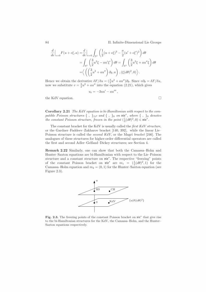
84 II. Infinite-Dimensional Lie Groups
d
dε
∣
∣
∣
ε=0F (u+ εξ, a) =
d
dε
∣
∣
∣
ε=0
∫
S1
(
12(u+ εξ)3 − a
2(u′ + εξ′)2
)
dθ
=∫
S1
(
32u2ξ − au′ξ′
)
dθ =∫
S1
(
32u2ξ + au′′ξ
)
dθ
=⟨
((
32u2 + au′′
)
∂θ, a
)
, (ξ(dθ)2, 0)⟩
.
Hence we obtain the derivative δF/δu = (32u
2 + au′′)∂θ. Since v∂θ = δF/δu,now we substitute v = 3
2u2 + au′′ into the equation (2.21), which gives
ut = −3uu′ − au′′′ ,
the KdV equation.
Corollary 2.21 The KdV equation is bi-Hamiltonian with respect to the com-patible Poisson structures , LP and , 0 on vir
∗, where , 0 denotesthe constant Poisson structure, frozen in the point (1
2 (dθ)2, 0) ∈ vir∗.
The constant bracket for the KdV is usually called the first KdV structure,or the Gardner–Faddeev–Zakharov bracket [140, 392], while the linear Lie–Poisson structure is called the second KdV, or the Magri bracket [246]. Theanalogues of these structures for higher-order differential operators are calledthe first and second Adler–Gelfand–Dickey structures; see Section 4.
Remark 2.22 Similarly, one can show that both the Camassa–Holm andHunter–Saxton equations are bi-Hamiltonian with respect to the Lie–Poissonstructure and a constant structure on vir
∗. The respective “freezing” pointsof the constant Poisson bracket on vir
∗ are m1 = (12 (dθ)2, 1) for the
Camassa–Holm equation and m2 = (0, 1) for the Hunter–Saxton equation (seeFigure 2.3).
KdV u(θ)(dθ)20
HS CH
a
Fig. 2.3. The freezing points of the constant Poisson bracket on vir∗ that give rise
to the bi-Hamiltonian structures for the KdV, the Camassa–Holm, and the Hunter–Saxton equations respectively.

2. Diffeomorphisms of the Circle and the Virasoro–Bott Group 85
Remark 2.23 The bi-Hamiltonian nature of the KdV equation allows one toobtain the whole hierarchy of the KdV Hamiltonians via the Lenard–Magrischeme discussed in the introduction.
Namely, consider the linear combination of the Poisson brackets for theKdV: the Virasoro Lie–Poisson and the constant ones:
, λ := , LP + λ2 , 0 .
Since the corresponding brackets are compatible, , λ defines a Poissonbracket for all λ ∈ R, which is the usual Lie–Poisson bracket on vir
∗ shiftedin the direction of m0 = (1
2 (dθ)2, 0) ∈ vir∗. (Note that one uses here the
parameter λ2 rather than λ for the expansion below to have a simpler form.)Recall that we think of the dual space vir
∗ = a∂2θ + u(θ) as the space of
Hill’s operators. The monodromy of a differential operator ∂2θ + u(θ), which
is a matrix in SL(2,R), changes to a conjugate matrix under the Virasorocoadjoint action (see Theorem 2.12). Therefore, the trace of the monodromyis a Casimir function for the Poisson bracket , LP on (the hyperplane a = 1in) the dual space vir
∗. The same reasoning allows one to obtain the followingresult.
Lemma 2.24 Let Mλ denote the monodromy of the differential operatord2
dθ2 + u(θ) − λ2. Then the function
hλ := log(tr(Mλ))
is a Casimir function for the Poisson bracket , λ on the space vir∗.
Indeed, , λ is the usual Lie–Poisson bracket on vir∗ shifted in the direction
of m0 = (0·∂2θ +1/2) ∈ vir
∗, and so, instead of the Lie–Poisson Casimir tr(M),we can use the shifted Casimir tr(Mλ) or any function of it, in particular,log(tr(Mλ)).
Finally, by expanding hλ into a power series in λ−1 one produces firstintegrals of the KdV equation:
hλ = 2πλ−∞∑
n=1
h2n−1λ1−2n ,
where
h1 =12
∫
S1u dθ, h3 =
18
∫
S1u2 dθ, h5 =
116
∫
S1(u3 − 1
2(u′)2) dθ, . . . ;
see, e.g., [31, 37].
86 II. Infinite-Dimensional Lie Groups
2.6 Bibliographical Notes
The cohomology of the Lie algebra of vector fields on the circle was computedby Gelfand and Fuchs in [143], where the term Virasoro algebra was coinedafter the paper [376] (see also [118, 138]). The Bott cocycle on the groupDiff(S1) first appeared in [53].
The group Diff(S1) (and hence the Virasoro group) does not admit anatural complexification, i.e., a group corresponding to the complexified Liealgebra Vect(S1)C; see [205, 322] and Example I.1.25. However, for a cone inthis complex Lie algebra consisting of those vector fields that “point outside ofthe circle,” there exists a semigroup. This annulus semigroup appeared in thepapers of Neretin [291] and Segal [343]. For more details on representationsand applications of the Virasoro group and algebra see [292, 322, 153].
The classification of the coadjoint orbits of the Virasoro group can befound in the literature under different guises: as a classification of projectivestructures on the circle by Kuiper [223], as a classification of Hill’s operatorsby Lazutkin and Pankratova [233], and in the present form, as Virasoro orbits,in the papers by Kirillov [202, 205] and Segal [342]; see also [164, 304, 388, 32].The adjoint orbits of the diffeomorphism group of the circle were described in[164].
The Virasoro coadjoint orbit Diff(S1)/S1 can also be understood as theuniversal Teichmuller space [326]; cf. [284, 285]. Curvatures of a Kahler met-ric on this orbit were described in [208], while its complex Hilbert manifoldstructure is discussed in [338, 363]. The Virasoro group itself admits a com-plex structure and can be viewed as a holomorphic C
∗-bundle over its orbitDiff(S1)/S1 [236].
There is a vast literature related to the geometry and Hamiltonian prop-erties of the KdV equation, which is one of the key examples in any bookon soliton theory. The description of the KdV equation, as well as its super-analogue, as an Euler–Arnold equation on the Virasoro group with respect tothe L2-metric can be found in [305, 344, 346]. More general, H1-type, metricson this group were considered in [268, 189, 192], and we followed the latterpaper in our exposition. Regularity properties of the Riemannian exponentialmaps for these and other Sobolev metrics on the Virasoro and the diffeomor-phism groups are described in [73, 74].
The Adler–Gelfand–Dickey structures [3, 141, 142] are the generalizationsof the KdV Poisson structures from Hill’s operators to linear differential op-erators of higher order, and we discuss them in Section 4.
For the algebro-geometric approach to constructing solutions of the KdVequation we address the reader to [216]; the description of the correspond-ing infinite-dimensional Grassmann manifolds can be found in [347] and thereferences therein. Various analytical aspects of the KdV theory, its spectraltheory, and the angle-action variables are discussed in the book [182]. Thegeometry related to the KAM theory for near-integrable Hamiltonian systems,
2. Diffeomorphisms of the Circle and the Virasoro–Bott Group 87
applied in the infinite-dimensional context, e.g., to the KdV-type equations,is discussed in [224, 182].
88 II. Infinite-Dimensional Lie Groups
3 Groups of Diffeomorphisms
Diffeomorphism groups constitute one of the most intriguing classes of infinite-dimensional Lie groups. They often serve as configuration spaces for variousequations of fluid and gas dynamics. In this section, our main objects of studyare the groups of volume-preserving diffeomorphisms, in particular their geom-etry and coadjoint orbits. The Euler geodesic equations for such groups andfor their generalizations deliver the Euler equations for ideal incompressiblefluids on manifolds, as well as the equations of compressible fluids and mag-netohydrodynamics. We also discuss how invariants of the coadjoint action ofcertain diffeomorphism groups are related to knot theory and to the symplec-tic structure on the space of immersed curves in R
3.
3.1 The Group of Volume-Preserving Diffeomorphismsand Its Coadjoint Representation
Let M be an n-dimensional compact manifold (possibly with boundary) andlet µ be a volume form on M .
Definition 3.1 The group of volume-preserving diffeomorphisms of the mani-fold M consists of all diffeomorphisms of M preserving the volume form µ:
SDiff(M) = ϕ ∈ Diff(M) | ϕ∗µ = µ ,
where the group multiplication is the composition of diffeomorphisms. (When-ever this group of diffeomorphisms is not connected, our notation SDiff standsfor the connected component of the identity of this group.)
Exercise 3.2 The corresponding Lie algebra SVect(M) consists ofdivergence-free vector fields on M :
SVect(M) = ξ ∈ Vect(M) | Lξµ = 0 and ξ is tangent to ∂M ,
where the algebra commutator is the negative of the Lie bracket of two vectorfields: [ξ, η] = −Lξη; cf. Example I.2.2.
It turns out that the (smooth part of the) dual of the Lie algebra SVect(M)has a natural geometric description.
Proposition 3.3 The smooth part of the dual of the Lie algebra SVect(M)is naturally identified with the space Ω1(M)/dΩ0(M) of smooth 1-forms onM modulo exact 1-forms on M . The pairing is as follows:
〈ξ, [u]〉 =∫
M
ιξu ∧ µ ,
where u ∈ Ω1(M) is any 1-form from the coset [u].
3. Groups of Diffeomorphisms 89
In the coadjoint representation, a diffeomorphism ϕ ∈ SDiff(M) acts by“change of coordinates”: it sends a coset [u] ∈ Ω1(M)/dΩ0(M) to the coset[(ϕ−1)∗u]. Accordingly, the coadjoint action of SVect(M) on Ω1(M)/dΩ0(M)is given by the negative of the Lie derivative:
ad∗ξ : [u] → −[Lξu]
for any divergence-free vector field ξ on M .
Proof. Assume first that the manifold M has no boundary. Note thatdivergence-free vector fields on M are in one-to-one correspondence with thespace of all closed (n − 1)-forms on M . Indeed, any vector field ξ on Mdefines an (n − 1)-form νξ via interior product with the volume form on M :νξ = ιξµ. Moreover, this form νξ is closed for a divergence-free field ξ, since0 = Lξµ = dιξµ+ ιξdµ = dνξ.
The pairing between Ω1(M)/dΩ0(M) and SVect(M) can now be rewrittenas
〈ξ, [u]〉 =∫
M
u ∧ νξ
for any representative 1-form u. Two different representatives u and u differby a differential df and give the same pairing. Indeed, since the form νξ isclosed, so is df ∧ νξ. Then the Stokes formula gives
〈ξ, df〉 =∫
M
df ∧ νξ =∫
M
d(f ∧ νξ) = 0
for M without boundary.In the case of a manifold M with boundary ∂M , the restriction of the
closed (n − 1)-form νξ vanishes on ∂M . Then the application of the Stokesformula gives the same result as above. Thus, the pairing between SVect(M)and Ω1(M)/dΩ0(M) is indeed well defined.
Finally, recall that in the adjoint representation, the group Diff(M) actson its Lie algebra Vect(M) by coordinate changes: Adϕ(ξ) = ϕ∗ξϕ−1. Hencewe obtain
〈ξ,Ad∗ϕ[u]〉 = 〈Adϕ−1 ξ, [u]〉 =
∫
M
u ∧ ιϕ−1∗ ξµ =
∫
M
(ϕ−1)∗u ∧ ιξ(
(ϕ−1)∗µ)
.
Since ϕ preserves the volume form µ, we have Ad∗ϕ[u] = [(ϕ−1)∗u]. The state-
ment on infinitesimal coadjoint action of the Lie algebra SVect(M) readilyfollows.
Note also that the actions Ad∗ and ad∗ are well defined on the cosets,since changes of coordinates commute with taking d.
90 II. Infinite-Dimensional Lie Groups
Exercise 3.4 Complete the proof of Proposition 3.3 in the case of a manifoldM with boundary. (Hint: in order to show that the restriction of the closed(n − 1)-form νξ vanishes on ∂M , use the fact that the field ξ is tangent to∂M .)
3.2 The Euler Equation of an Ideal Incompressible Fluid
Imagine an ideal incompressible fluid occupying a domain M in Rn.
Definition 3.5 The fluid motion is described by a velocity field v(t, x) anda pressure function p(t, x) that satisfy the classical Euler equation of an idealincompressible fluid:
∂tv + (v,∇)v = −∇p , (3.22)
where div v = 0 and the field v is tangent to the boundary of M . The functionp is defined uniquely modulo an additive constant by the conditions that vhave zero divergence and be tangent to the boundary.
In Euclidean coordinates, equation (3.22) reads
∂tvi +n∑
j=1
vj∂vi
∂xj= − ∂p
∂xi.
The same equation describes the motion of an ideal incompressible fluidfilling an arbitrary Riemannian manifold M equipped with a volume form µ.In the latter case, v is a divergence-free vector field on M , the notation (v,∇)vstands for the Riemannian covariant derivative ∇vv of the field v in the di-rection of itself, and div v is taken with respect to the volume form µ.
Remark 3.6 Equation (3.22) has a natural interpretation as a geodesic equa-tion [12, 18]. Indeed, consider the flow (t, x) → φ(t, x) defined by the velocityfield v(t, x), which describes the motion of fluid particles:
∂tφ(t, x) = v(t, φ(t, x)), φ(0, x) = x
for all x ∈ M . The chain rule immediately gives
∂2t φ(t, x) = (∂tv + (∂xv)(∂tφ))(t, φ(t, x)) = (∂tv + (v,∇)v)(t, φ(t, x)) ,
and hence the Euler equation (3.22) is equivalent to
∂2t φ(t, x) = −(∇p)(t, φ(t, x)),
while the incompressibility condition div v = 0 becomes det(∂xφ(t, x)) = 1.The latter form of the Euler equation (for a smooth flow φ(t, x)) says that theacceleration of the flow is given by the gradient of a function. Therefore this

3. Groups of Diffeomorphisms 91
acceleration is L2-orthogonal to the set of volume-preserving diffeomorphisms(or, rather, to its tangent space, the space of divergence-free fields):
∫
M
(∇p, ξ)µ = 0
for all divergence-free vector fields ξ and all smooth functions p on M . In otherwords, the fluid motion φ(t, .) is a geodesic line on the set of volume-preservingdiffeomorphisms of the domain M with respect to the induced L2-metric onthe group SDiff(M). This L2-metric is the kinetic energy of the fluid flow:for a velocity field v its energy is E(v) = 1
2
∫
M(v, v)µ. Fluid flows describe
geodesics on the group SDiff(M), since they extremize this energy accordingto the least action principle.
In the case of an arbitrary Riemannian manifold M , the Euler equationdefines the geodesic flow on the group of volume-preserving diffeomorphisms ofM with respect to the right-invariant L2-metric on SDiff(M); see [12, 96, 24].
3.3 The Hamiltonian Structure and First Integrals of the EulerEquations for an Incompressible Fluid
The geodesic properties of the Euler equation can also be described withinthe Hamiltonian framework. The latter turns out to be useful in establishingnumerous conservation laws for flows of an ideal fluid.
Consider the Lie algebra SVect(M) of divergence-free vector fields on acompact manifold M and its dual space SVect(M)∗ = Ω1(M)/dΩ0(M) of1-forms modulo exact 1-forms. This algebra is equipped with the L2 quadraticform
(ξ1, ξ2)SVect =∫
M
(ξ1, ξ2)µ , (3.23)
which is induced by fixing a Riemannian metric ( , ) on the manifold M . Thecorresponding inertia operator
A : SVect(M) → Ω1(M)/dΩ0(M)
sends a vector field ξ to the coset [u] of the 1-form u that is obtained from thefield ξ by “raising indices” with the help of the metric: u( . ) = (ξ, . ). (In R
n
with the standard Euclidean metric, the inertia operator A maps a vector fieldξ =
∑
ξi∂/∂xi to the 1-form uξ =∑
ξidxi.) Since the Riemannian metric isnondegenerate, so is the map A : ξ → [u]. Note that in each coset [u] thereis a unique representative 1-form, which is obtained by raising indices from adivergence-free field.
Lemma 3.7 Let H be the quadratic Hamiltonian on Ω1(M)/dΩ0(M) definedby the inertia operator A:

92 II. Infinite-Dimensional Lie Groups
H([u]) =12〈A−1[u], [u]〉 .
Then the Hamiltonian equation on Ω1(M)/dΩ0(M) for the Hamiltonian func-tion −H with respect to the Lie–Poisson bracket is the following:
d
dt[u] = −Lξ[u] , (3.24)
where [u] is the coset of the 1-form u related to the divergence-free field ξ withthe help of the metric, u( . ) = (ξ, . ).
Proof. Recall from Corollary I.4.11 that the Hamiltonian equation withrespect to the function −H is given by
d
dt[u] = − ad∗
(−A−1[u])[u] = ad∗A−1[u][u] .
The coadjoint action of the Lie algebra SVect(M) on its dual is given by thenegative of the Lie derivative, so that we get equation (3.24).
Corollary 3.8 The Hamiltonian equation (3.24) is equivalent to the Eulerequation for an ideal incompressible fluid on the manifold M .
Proof. Rewriting equation (3.24) in terms of the coset representative, the1-form u ∈ [u], gives
∂tu = −Lξu− dp (3.25)
for a time-dependent function p. Passing back to vector fields, i.e., applyingA−1 to both sides of equation (3.25), we get our final equation
∂tξ = −(ξ,∇)ξ −∇p .
(Here we use the fact that “raising indices” sends the covariant derivative(ξ,∇)ξ to the Lie derivative Lξu up to a full differential; see, e.g., [24].) Thelatter is the Euler equation for an ideal incompressible fluid on M , where p isinterpreted as the pressure function.
This description of the dual space and the Euler hydrodynamics equationallows one to describe certain first integrals of the fluid motion practicallywithout calculations. Indeed, start with the following proposition, which pro-vides certain Casimir functions for the coadjoint action of the group SDiff(M).Let M be a compact manifold equipped with a volume form µ.
Proposition 3.9 ([307]) If the manifold M is of odd dimension 2m+1, thenthe function
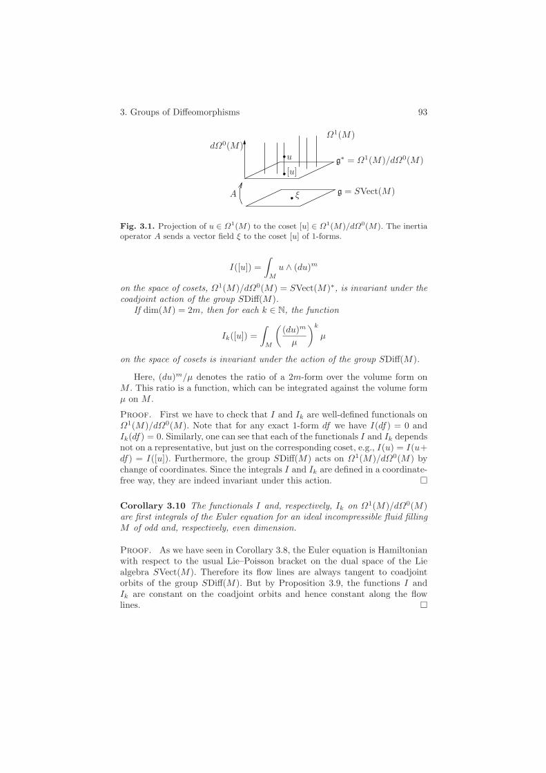
3. Groups of Diffeomorphisms 93
A
[u]
u
g = SVect(M)
Ω1(M)dΩ0(M)
g∗ = Ω1(M)/dΩ0(M)
ξ
Fig. 3.1. Projection of u ∈ Ω1(M) to the coset [u] ∈ Ω1(M)/dΩ0(M). The inertiaoperator A sends a vector field ξ to the coset [u] of 1-forms.
I([u]) =∫
M
u ∧ (du)m
on the space of cosets, Ω1(M)/dΩ0(M) = SVect(M)∗, is invariant under thecoadjoint action of the group SDiff(M).
If dim(M) = 2m, then for each k ∈ N, the function
Ik([u]) =∫
M
(
(du)m
µ
)k
µ
on the space of cosets is invariant under the action of the group SDiff(M).
Here, (du)m/µ denotes the ratio of a 2m-form over the volume form onM . This ratio is a function, which can be integrated against the volume formµ on M .
Proof. First we have to check that I and Ik are well-defined functionals onΩ1(M)/dΩ0(M). Note that for any exact 1-form df we have I(df) = 0 andIk(df) = 0. Similarly, one can see that each of the functionals I and Ik dependsnot on a representative, but just on the corresponding coset, e.g., I(u) = I(u+df) = I([u]). Furthermore, the group SDiff(M) acts on Ω1(M)/dΩ0(M) bychange of coordinates. Since the integrals I and Ik are defined in a coordinate-free way, they are indeed invariant under this action.
Corollary 3.10 The functionals I and, respectively, Ik on Ω1(M)/dΩ0(M)are first integrals of the Euler equation for an ideal incompressible fluid fillingM of odd and, respectively, even dimension.
Proof. As we have seen in Corollary 3.8, the Euler equation is Hamiltonianwith respect to the usual Lie–Poisson bracket on the dual space of the Liealgebra SVect(M). Therefore its flow lines are always tangent to coadjointorbits of the group SDiff(M). But by Proposition 3.9, the functions I andIk are constant on the coadjoint orbits and hence constant along the flowlines.

94 II. Infinite-Dimensional Lie Groups
Remark 3.11 Being Casimirs, the functionals I and Ik give conservationlaws for any Hamiltonian equation on SVect(M)∗ = Ω1(M)/dΩ0(M) withrespect to the Lie–Poisson bracket. In particular, the functionals I and Ik
are first integrals of the Euler equation for an arbitrary metric on M . Theseintegrals manifest the “kinematic symmetries” of the hydrodynamical system,while the energy is an invariant related to the system’s “dynamics.”
Example 3.12 Specifying to the case of a three-dimensional domain M ⊂R
3, we see that the function
I(ξ) =∫
M
u ∧ du ,
where u and ξ are related by means of the Euclidean metric, is a first integralof the Euler equation. A short direct calculation allows one to rewrite I(ξ) inthe form
I(ξ) =∫
M
(ξ, curl ξ) d3x .
The latter integral has a natural geometric meaning of helicity of the vectorfield curl ξ:
Definition 3.13 Let M be a three-dimensional compact manifold with avolume form µ and suppose that the second de Rham cohomology group ofM vanishes: H2(M,R) = 0. Then, if η is a divergence-free vector field on Mtangent to the boundary of M , the corresponding 2-form ωη = ιηµ is closed,and hence exact. So we can find a 1-form α on M such that ωη = dα. Thehelicity of the vector field η is defined by
Hel(η) =∫
M
α ∧ dα =∫
M
d−1(ωη) ∧ ωη .
Exercise 3.14 Show that the helicity does not depend on the ambiguity inthe definition of the 1-form α = d−1ωη.
The helicity of a vector field η has a topological interpretation as the asymp-totic Hopf invariant, or “average linking number” of the trajectories of thevector field η (see [16, 24, 269] for details).
Example 3.15 Similarly, specifying to the case of a two-dimensional domainM ⊂ R
2, we find infinitely many first integrals of the Euler equation, namely
Ik(ξ) =∫
M
(curl ξ)kd2x ,
where curl ξ := ∂ξ1∂x2
− ∂ξ2∂x1
is the vorticity function on M ⊂ R2.

3. Groups of Diffeomorphisms 95
Remark 3.16 The functions I and Ik on Ω1(M)/dΩ0(M) are invariant un-der the coadjoint action of the group SDiff(M). However, it should be notedthat they do not form a complete set of invariants of the coadjoint repre-sentation. One can construct parametrized families of orbits on which thesefunctions take the same values.
Exercise 3.17 Prove that for an odd-dimensional manifold M not only isthe integral I([u]) over the entire manifold M invariant under the coadjointaction of SDiff(M), but so are the integrals
IC([u]) =∫
C
u ∧ (du)m
over every set C invariant with respect to the vorticity vector field η = curl ξ.This field is defined for any odd n = 2m+1 as the kernel field of the 2m-form(du)m on the manifold M : ιηµ = (du)m, where the 1-form u is related to thevector field ξ with the help of the Riemannian metric.
Certain nonanalytic invariants of the coadjoint action on SVect(M)∗ canbe extracted from the ergodic description of the helicity functional as theaverage of pairwise linkings of the trajectories of the field η; see [16]. In theeven-dimensional case, slightly more general invariants than Ik are obtainedby replacing ((du)m/µ)k with f((du)m/µ) for any function f : R → R.
The full classification of the coadjoint orbits of the diffeomorphism groupsis still an open problem [24, 205]. Below we show that a complete set of suchinvariant functionals defined on singular coadjoint orbits of this group wouldinclude all knot and link invariants!
3.4 Semidirect Products: The Group Setting for an IdealMagnetohydrodynamics and Compressible Fluids
It is curious to note that the similarity pointed out by V. Arnold betweenthe Euler top on the group SO(3) and the Euler ideal fluid equations onSDiff(M) has a “magnetic analogue”: a parallelism between the Kirchhoffand magnetohydrodynamics (MHD) equations; see the table in Example 4.18of Chapter I.
The latter equations are both related to the groups that are semidirectproducts. The Kirchhoff equations for the motion of a rigid body in a fluidare associated with the group E(3) = SO(3) R
3 of Euclidean motions of thethree-dimensional space. In this group, a Euclidean motion is described by apair (a, b), a rotation a ∈ SO(3) and a translation by a vector b ∈ R
3, so thatthe group multiplication law between two such pairs,
(a2, b2) (a1, b1) = (a2a1, b2 + a2b1) ,
is determined by the consecutive application of motions.

96 II. Infinite-Dimensional Lie Groups
Similarly, magnetohydrodynamics is governed by the group SDiff(M)
SVect(M). Elements of the corresponding Lie algebra are pairs of divergence-free vector fields (v,B), which can be interpreted as the velocity field v andthe magnetic field B.
In the idealized setting, an inviscid incompressible fluid obeying hydro-dynamical principles transports a magnetic field. In turn, the medium itselfexperiences a reciprocal influence of the magnetic field. The evolution is de-scribed by the following system of Maxwell’s equations.
Definition 3.18 Consider an electrically conducting incompressible fluidthat fills some domain M ⊂ R
3 and transports a divergence-free magneticfield B. Then the evolution of the field B and of the fluid velocity field v isdescribed by the system of ideal magnetohydrodynamics (MHD) equations
∂tv = −(v,∇)v + (curl B) ×B −∇p ,∂tB = −LvB ,
where div B = div v = 0 with respect to the standard volume form µ = d3xin M and the coefficients are normalized by a suitable choice of units.
Here, the second equation is the definition of the “frozenness” of the mag-netic field B into the medium, and LvB denotes the Lie bracket of two vectorfields. (Note that a frozenness-type condition usually indicates the structureof a semidirect product in the corresponding symmetry group; cf. [253].) Theterm (curl B) × B represents the Lorentz force j × B, which acts on a unitcharge moving with velocity j in the magnetic field B. The motion of electriccharges produces the electrical current field j proportional to curl B.
Theorem 3.19 ([377, 253]) The magnetohydrodynamics equations are theEuler equations corresponding to the right-invariant metric on the groupSDiff(M) SVect(M) generated by the sum of the kinetic and magneticenergies
E(v,B) :=12
∫
M
[(v, v) + (B,B)] µ
on its Lie algebra of pairs (v,B).
A somewhat similar description is available for compressible fluids as well.Consider, for instance, barotropic gases or fluids, whose pressure is a fixedfunction of density.
Definition 3.20 The equations of motion of a barotropic gas (or fluid) on aRiemannian manifold M are given by
ρ ∂tv = −ρ (v,∇)v −∇h(ρ) ,∂tρ+ div(ρ · v) = 0 ,
(3.26)

3. Groups of Diffeomorphisms 97
where ρ ∈ C∞(M) is the density of the gas, the time-dependent vector field vis the velocity vector field, and h : C∞(M) → C∞(M) is the fixed correspon-dence between the density function ρ and the pressure function p = h(ρ). Theequations of barotropic gas dynamics usually correspond to a specific choiceof h(ρ) = const · ρa. For an ideal gas, a = 1 + 2
D , where D is the number ofdegrees of freedom of a molecule. For instance, for monatomic gases (argon,krypton) D = 3 and a = 5/3, while for diatomic gases (such as nitrogen,oxygen, and hence approximately for air) D = 5 and a = 7/5.
To describe these equations as Euler equations we note first that the mainplayer here will be the group Diff(M) of all (not only volume-preserving)diffeomorphisms of a manifold M . Its Lie algebra Vect(M) consists of allsmooth vector fields on M .
For the barotropic gas dynamics we need a certain extension of this group.Namely, consider the semidirect product group G = Diff(M) C∞(M). Thisis the group consisting of pairs (ϕ, f), where ϕ is a diffeomorphism of themanifold M , and f is a smooth function. The product on the group Diff(M)
C∞(M) is given by
(ϕ, f) · (ψ, g) = (ϕ ψ,ϕ∗g + f) ,
where ϕ∗g = g ϕ−1 denotes the pushforward of the function g by the dif-feomorphism ϕ (or, equivalently, the pullback by ϕ−1). The smoothness ofthe group product on Diff(M) C∞(M) follows from that of the product onDiff(M) and that of the action of Diff(M) on C∞(M).
ϕ
Diff(M)
(ϕ, f)
ϕ ψ
(ϕ ψ,ϕ∗g + f)
ψ
(ψ, g)
Diff(M) C∞(M)
Fig. 3.2. As a topological space, the semidirect product Diff(M) C∞(M) is theproduct of the spaces Diff(M) and C∞(M). The group structure is not a directproduct, but is twisted by the action of Diff(M) on C∞(M) by pushforwards.
The Lie algebra g of the group Diff(M) C∞(M) is also a semidirectproduct, the Lie algebra Vect(M) C∞(M). As a vector space, it is thedirect sum Vect(M) ⊕ C∞(M), while the Lie algebra structure on this spaceencompasses the natural action of vector fields on functions.
98 II. Infinite-Dimensional Lie Groups
Exercise 3.21 Find explicit formulas for the adjoint representation of thegroup Diff(M) C∞(M) and the Lie bracket of its algebra. (Hint: for moredetails on this and the following exercises, see Appendix A.7.)
To describe the corresponding dual space, we return first to the groupDiff(M) of all diffeomorphisms, whose Lie algebra Vect(M) consists of allsmooth vector fields.
Exercise 3.22 Show that the (smooth) dual of the Lie algebra Vect(M) canbe naturally identified with the space Ω1(M) ⊗C∞(M) Ω
n(M). Elements ofthis space are linear combinations of tensor products of 1-forms with n-formson M , where given a 1-form α and an n-form µ we identify the elementsf ·α⊗µ with α⊗ f ·µ for any smooth function f . The pairing between vectorfields on M and elements of this space Ω1(M) ⊗C∞(M) Ω
n(M) =: Vect(M)∗
is given by
〈ξ, α⊗ µ〉 =∫
M
(ιξα)µ .
The naturality of the pairing means that the coadjoint action of Diff(M) isthe change of coordinates by a diffeomorphism.
Now the smooth part of the dual of the semidirect product Lie algebraVect(M)C∞(M) can be identified with the space (Ω1(M)⊗C∞(M)Ω
n(M))⊕Ωn(M) via the pairing
〈(ξ, f), (α⊗ µ, ν)〉 =∫
M
(ιξα)µ+∫
M
fν .
Exercise 3.23 Show that the coadjoint action of the group Diff(M)C∞(M)on the space (Ω1(M) ⊗C∞(M) Ω
n(M)) ⊕Ωn(M) is given by
Ad∗(ϕ,f)−1(α⊗ η, ν) = (ϕ∗α⊗ ϕ∗η + ϕ∗df ⊗ ϕ∗ν, ϕ∗ν) . (3.27)
In order to define a dynamical system related to this group, we need someadditional data. Fix a Riemannian metric ( , ) and a volume form µ on themanifold M . Furthermore, fix a function h : C∞(M) → C∞(M) that assignsto a density ρ of the fluid its pressure h(ρ).
Define the Hamiltonian functional H : Vect(M) ⊕ C∞(M) → R by
H(ξ, ρ) =∫
M
(
12(ξ, ξ) ρ+ ρΦ(ρ)
)
µ ,
where Φ(ρ) is chosen such that ρ2Φ′(ρ) = h(ρ).
Exercise 3.24 Show that the Euler equation corresponding to the lift of theHamiltonian −H to the dual of the Lie algebra is exactly the Euler equationof a barotropic fluid. (The lift of H to the dual space is given by the inertiaoperator defined by the Riemannian metric, see details in Appendix A.7.)
3. Groups of Diffeomorphisms 99
Exercise 3.25 Find Casimir functions similar to the ones we discussed inthe case of the Euler equation of an ideal incompressible fluid. (Hint: in thecoordinate system “moving with the fluid” the equations of motion can bethought of as those for an incompressible fluid.)
Remark 3.26 Thus it turns out that the barotropic fluid equations also havean infinite number of conservation laws in the even-dimensional case, and atleast one first integral in the odd-dimensional case; see [24, 307].
The Hamiltonian approach allows one to apply the technique of Casimirfunctions to the stability study of barotropic fluids and ideal MHD systems:their dynamics take place on coadjoint orbits of the corresponding groups,and the Casimir functions help in describing the corresponding conditionalextrema of the Hamiltonians.
More general equations of compressible fluids include also the function ofentropy. The corresponding Lie group can be identified with the semidirectproduct G = Diff(M) (C∞(M) ⊕ C∞(M)): the first summand of the ex-tension stands for the density, while the second one represents the entropyfunction; see [90].
3.5 Symplectic Structure on the Space of Knotsand the Landau–Lifschitz Equation
Consider an embedding of the (oriented) circle S1 into Euclidean space R3,
i.e., a knot in R3. Associate to this curve a linear functional on the space
SVect(R3) of divergence-free fields in R3, that is, an element of the dual
space SVect(R3)∗, as follows. Take a compact oriented surface S ⊂ R3 such
that the oriented boundary of S coincides with the knot γ: ∂S = γ. Such a sur-face is called a Seifert surface for γ. Then to any vector field ξ ∈ Vect(R3) wecan associate its flux through the surface S. If the vector field ξ is divergence-free, the flux does not depend on the choice of the surface S, so that the curveγ defines a functional on the Lie algebra SVect(R3):
〈γ, ξ〉 = Flux(ξ)|S =∫
S
ιξµ , (3.28)
where µ = d3x is the standard volume form in R3; see Figure 3.3.
Remark 3.27 Obviously, the functional on the Lie algebra SVect(R3) de-fined by the curve γ does not lie in the smooth part of the dual of SVect(R3).But we can still associate to γ a coset of singular, rather than smooth, 1-formson R
3. Namely, given a Seifert surface S we consider the “δ-type” 1-form uS
supported on S, whose integral over any closed curve σ in R3 intersecting the
surface S transversally counts (with signs) the intersections of the curve σwith this surface S.

100 II. Infinite-Dimensional Lie Groups
Fig. 3.3. A Seifert surface for a knot defines the flux functional on vector fields.
Exercise 3.28 Verify that although the 1-form uS depends on the choice ofthe surface S, its coset [uS ] does not: the choice of another Seifert surface ˜Schanges the 1-form uS by a complete differential.
This coset [uS ] belongs to a closure Ω1(R3)/dΩ0(R3) of the smooth dualspace SVect(R3)∗ = Ω1(R3)/dΩ0(R3). Note that the latter space of all smooth1-forms modulo exact 1-forms is isomorphic to the space Z2(R3) of all smoothclosed 2-forms in R
3: The exterior derivative d takes any such coset of 1-formsto a closed 2-form without any loss of information, since H1(R3) = 0.
Alternatively, one can directly associate to the curve γ a singular closed2-form ωγ in R
3. This is the δ-type 2-form (called the de Rham current) sup-ported on γ. (More precisely, de Rham currents are, by definition, continuouslinear functionals on differential forms. The curve γ defines the current ωγ ,whose value on any smooth 1-form α on R
3 is 〈ωγ , α〉 =∫
γα. Similarly, the
current uS is defined by prescribing its value 〈uS , β〉 =∫
Sβ for any smooth
2-form β on R3.) The relation duS = ωγ between these currents exactly mani-
fests the relation ∂S = γ between a knot γ and its Seifert surface S.In this way, a knot γ in R
3 can be seen as an element of the (full) dual spaceto the Lie algebra of divergence-free vector fields on R
3. From this viewpoint,the coadjoint orbit through γ is the equivalence class of the knot γ undervarious isotopies. (Evidently, any isotopy of a knot γ ⊂ R
3 can be extended toa volume-preserving diffeomorphism of the ambient space R
3.) This leads tothe curious observation that knot invariants constitute a part of the coadjointinvariants of the whole Lie group SDiff(R3); see, e.g., [16, 24].
Let us extend our consideration from embedded to immersed closed curvesin R
3. The space C of such curves can be regarded as an infinite-dimensionalsymplectic manifold. Let γ = γ(S1) ⊂ R
3 be a closed immersed curve in R3,
and for now fix a parametrization θ of the circle S1. A tangent vector α to Cat γ is an infinitesimal variation of the curve γ, that is, a normal vector fieldattached to γ(S1).
Definition 3.29 The Marsden–Weinstein symplectic structure is the follow-ing 2-form ωMW on the space C of immersed closed curves in R
3 with a fixedvolume form µ. Its value on the two tangent vectors a and b to C at γ is given

3. Groups of Diffeomorphisms 101
by the oriented volume of the collar spanned along γ by the vectors a(θ) andb(θ); see Figure 3.4. Explicitly, for the chosen parametrization θ,
ωMW(a, b) :=∫
S1µ(a(θ), b(θ), γ′(θ))dθ =
∫
γ
ιbιa µ .
The latter integral shows that the value of ω does not depend on the parame-trization, i.e., ωMW is indeed a symplectic structure on the space of nonpara-metrized curves.
γ
Fig. 3.4. The value of the symplectic structure ωMW evaluated on two variations ofthe curve γ is the volume of the collar spanned by the variations.
Proposition 3.30 The Marsden–Weinstein symplectic structure on the spaceof embedded curves containing γ coincides with the natural Kirillov–Kostantsymplectic structure on the coadjoint orbit of the group SDiff(R3) through thecurve γ, regarded as an element of the dual space to SVect(R3).
Exercise 3.31 Prove this proposition. (Hint: see [255, 24].)
Remark 3.32 The same construction works for any three-dimensional mani-fold equipped with a volume form. In higher dimensions, a similar constructionallows one to define a symplectic structure on the space of closed immersedsubmanifolds of codimension 2. One can also prove its equivalence with theKirillov–Kostant symplectic structure on (“singular”) coadjoint orbits forSDiff(Mn), which are linear functionals on divergence-free vector fields inM , represented by “fluxes through” hypersurfaces in M bounded by thesesubmanifolds; cf. [156].
Returning to the 3D case, we are going to make use of not only the volumeform, but also the Euclidean structure in R
3. Define the following “energy”

102 II. Infinite-Dimensional Lie Groups
function H on the space of immersed closed curves that assigns to a loopγ ∈ C its length:
H(γ) =∫
S1‖γ′(θ)‖ dθ =
∫
S1
√
(γ′(θ), γ′(θ)) dθ .
Proposition 3.33 The Hamiltonian equation corresponding to this energyfunction H with respect to the Marsden–Weinstein symplectic structure isgiven by the binormal (or filament) equation
∂tγ = γ′ × γ′′ (3.29)
in the arc-length parameter θ, see Figure 3.5. (Here, γ′ denotes the derivative∂∂θγ, and in the arc-length parametrization ‖γ′(θ)‖ = 1 for all θ ∈ S1.)
γ′
γ′′
∂tγ = γ′ × γ′′
γ
Fig. 3.5. The binormal equation describes the movement of a curve in R3 in the
direction ∂tγ = γ′ × γ′′.
Exercise 3.34 Prove this proposition. Show also that if θ is not arc-length,then the corresponding Hamiltonian equation becomes
∂tγ = k(θ, t)γ′ × γ′′ , (3.30)
where k(θ, t) is the curvature of the curve at the point θ at time t.(Hint: For the functional H(γ) in the arc-parametrization, the variational
derivative (i.e., the “gradient” of H in the space of curves C) is δH/δγ =−(length of γ)−1 γ′′. This can be thought of as a vector field normal to γ. Inturn, the Marsden–Weinstein symplectic structure at γ ∈ C can be regardedas the symplectic structure averaged from all two-dimensional planes normalto the loop γ. Then to obtain the corresponding Hamiltonian field vH , whichis the skew-gradient of H, we have to rotate the above gradient field δH/δγ byπ/2 around each tangent vector γ′(θ): if Jγ(∗) = γ′ × ∗ is the correspondingrotation operator, we get
vH = Jγ(δH/δγ) = −(length of γ)−1 γ′ × γ′′. )
3. Groups of Diffeomorphisms 103
Notice that the binormal vector γ′ × γ′′ is, in particular, orthogonal to γ′,and hence the evolution of the curve γ does not change the length of γ, i.e.,the Hamiltonian is indeed preserved.
This equation is also called the da Rios or localized induction approxima-tion (LIA) equation; see the nice survey [331]. It can also be obtained fromthe three-dimensional Euler equation (3.22) by keeping only “local terms” inthe corresponding evolution law for a vortex filament; see, e.g., [139].
Remark 3.35 Equation (3.29) is equivalent to the Heisenberg magnetic chainequation. Namely, set L = γ′. Then equation (3.29) becomes
∂tL = ∂tγ′ = γ′′ × γ′′ + γ′ × γ′′′ = γ′ × γ′′′ ,
so that we get∂tL = L× L′′ , (3.31)
which is also the simplest form of the Landau–Lifschitz equation.
Remark 3.36 The Heisenberg magnetic chain (or Landau–Lifschitz)equation has another interpretation as the Euler equation for a cer-tain left-invariant sub-Riemannian metric on the loop group LSO(3) =C∞(S1,SO(3)). The Hamiltonian formulation is as follows. Let us identifythe Lie algebra Lso(3) = C∞(S1, so(3)) with the smooth part of its dualLso(3)∗ via the pairing
〈X,Y 〉 = −∫
S1tr(X(θ)Y (θ)) dθ .
Now instead of defining an inertia operator A : Lso(3) → Lso(3)∗ we definethe following noninvertible self-adjoint operator B : Lso(3)∗ → Lso(3) actingin the opposite direction: B(Y ) = −Y ′′. (If B were invertible, it would havethe meaning of the inverse of the corresponding inertia operator: B = A−1.)The corresponding Hamiltonian function on the dual space Lso(3)∗ requiresonly the operator B for its definition and it is given by
H(Y ) :=12〈Y,B(Y )〉 = −1
2〈Y, Y ′′〉 =
12〈Y ′, Y ′〉
for Y ∈ Lso(3)∗.The image of B in Lso(3) is the subspace n0 of so(3)-valued functions on
the circle with zero mean. On this hyperplane n0 ⊂ Lso(3) the operator Bcan be inverted, and this gives rise to the so called H−1-metric
E(X) =12〈∂−1
θ X, ∂−1θ X〉 ,
since it is given by the squared L2-norm of the antiderivative ∂−1θ X for func-
tions X with zero mean, X ∈ n0 ⊂ Lso(3).

104 II. Infinite-Dimensional Lie Groups
Note that the quadratic form on the subspace n0 does not extend to a left-invariant Riemannian metric on a subgroup of LSO(3). Indeed, this subspacen0 ⊂ Lso(3) does not form a Lie subalgebra: the bracket of two loops with zeromean does not necessarily have zero mean. The subspace n0 of the tangentspace at the identity id ∈ LSO(3) generates a left-invariant distribution onthe group LSO(3), and we can extend the quadratic form E(X) from n0 to ametric on this distribution. This is an example of an infinite-dimensional non-integrable distribution on a group with a left-invariant sub-Riemannian met-ric. Normal geodesics for this metric are described by the same Hamiltonianpicture as for a left-invariant Riemannian metric on the group, i.e., by theHeisenberg magnetic chain (or Landau–Lifschitz) equation (3.31).
Note also that the same Hamiltonian equation on Lso(3)∗ can be obtainedfrom an invertible operator B := id +B, i.e., for B(Y ) := Y−Y ′′, which definesa left-invariant Riemannian metric on the group LSO(3); see [7]. Indeed, theaddition of the identity inertia operator does not change the Hamiltoniandynamics on the orbits, since the latter operator corresponds to the Killingform, and hence on each coadjoint orbit the new Hamiltonian differs from theold one by a constant.
Exercise 3.37 Show that the Landau–Lifschitz equation (3.31) is the Eulerequation for the energy E (or, equivalently, for the Hamiltonian function H).
Derive the Landau–Lifschitz equation with the same Hamiltonian H forthe loops in any semisimple Lie algebra g, where − tr(XY ) is replaced by theKilling form on g.
Remark 3.38 One can rewrite the binormal equations in the Frenet frame forγ as evolution equations for the curvature k(θ, t) and torsion τ(θ, t). Curiously,by passing to the new functions “velocity” v := τ and “energy density” ρ := k2
one obtains exactly the equations of a 1-dimensional barotropic fluid for aspecific function h relating density and pressure; see [370].
Exercise 3.39 Find this function h(ρ) corresponding to the binormalequation.
Another important feature of the binormal equation was observed byHasimoto [158]. He found the transformation
ψ(θ, t) = k(θ, t) exp
(
i ·∫ θ
0
τ(η, t)dη
)
,
which sends the binormal equation to the nonlinear Schrodinger equation
−i ∂tψ = ψ′′ +12|ψ|2ψ
for a complex-valued wave function ψ : S1 → C. The latter equation isknown to be a completely integrable (bi-Hamiltonian) infinite-dimensional
3. Groups of Diffeomorphisms 105
system (see, e.g., [90]). And so is the binormal equation, since the Hasimototransformation respects the corresponding Poisson and symplectic structures;see [232, 65]. A direct relation between the Schrodinger equation and thebarotropic fluid equation is described in [360].
3.6 Diffeomorphism Groups as Metric Spaces
In this section we sidestep slightly from our main theme, the coadjoint orbitsof the group of diffeomorphisms, and take a look at the geometry of the dif-feomorphism groups themselves. We discuss without proofs various peculiarproperties of the groups of volume-preserving and Hamiltonian diffeomor-phisms.
Consider a volume-preserving diffeomorphism of a bounded domain andregard it as a final fluid configuration for a fluid flow starting at the identitydiffeomorphism. In order to reach the position prescribed by this diffeomor-phism, every fluid particle has to move along some path in the domain. Thedistance of this diffeomorphism from the identity in the diffeomorphism groupis the averaged characteristic of the path lengths of the particles.
It turns out that the geometry of the groups of volume-preserving dif-feomorphisms of two-dimensional manifolds differs drastically from that ofhigher-dimensional ones. This difference is due to the fact that in three (andmore) dimensions there is enough space for particles to move to their finalpositions without hitting each other. On the other hand, the motion of theparticles in the plane might necessitate their rotations about one another.The latter phenomenon of “braiding” makes the system of paths of particlesin 2D necessarily long, in spite of the boundedness of the domain. The distinc-tion between different dimensions can be formulated in terms of properties ofSDiff(M) as a metric space.
Recall that on a Riemannian manifold M the group SDiff(M) of volume-preserving diffeomorphisms is equipped with the right-invariant L2-metric,which is defined at the identity by the L2-energy of vector fields.
Definition 3.40 To any smooth path φ(t, .) | 0 ≤ t ≤ 1 on the groupSDiff(M), i.e., to a family of volume preserving diffeomorphisms, we associateits (L2-) length:
φ(t, .) :=∫ 1
0
(∫
Mn
|∂tφ(t, x)|2µ)1/2
dt.
Then the distance between two fluid configurations ϕ,ψ ∈ SDiff(M) is theinfimum of the lengths of all paths in SDiff(M) connecting them:
distSDiff(ϕ,ψ) = inf φ(t, .) ,
where the φ(0, .) = ϕ and φ(1, .) = ψ. It is natural to define the (L2-) diameterof the group SDiff(M) as the supremum of distances between any two of itselements:

106 II. Infinite-Dimensional Lie Groups
diam ( SDiff(M) ) = supϕ,ψ∈SDiff(M)
distSDiff(ϕ,ψ).
Theorem 3.41 ([355, 357]) For a unit n-dimensional cube Mn where n ≥3, the diameter of the group of smooth volume-preserving diffeomorphismsSDiff(Mn) is finite in the right-invariant metric distSDiff and it is boundedabove as follows:
diam ( SDiff(Mn) ) ≤ 2√
n
3.
Finiteness of the diameter holds for an arbitrary simply connected mani-fold M of dimension three or higher. The two-dimensional case is completelydifferent:
Theorem 3.42 ([100]) For an arbitrary manifold M of dimension n = 2,the diameter of the group SDiff(M) is infinite.
Note that the diameter in the case n ≥ 3 can become infinite if the fun-damental group of M is nontrivial [100]. On the other hand, in the two-dimensional case the infiniteness of the diameter is of “local” nature. Themain difference between the geometries of the groups of diffeomorphisms intwo and three dimensions is based on the observation that for a long pathon SDiff(M3) that twists the particles in space, there always exists a “short-cut” untwisting them by making use of the third coordinate. One can com-pare this with the corresponding linear problems: π1(SL(2,R)) = Z, whileπ1(SL(n,R)) = Z/2Z for n ≥ 3. (Such a linear problem arises if we associateto a diffeomorphism in SDiff(M) and some fixed point in M the Jacobi matrixof the diffeomorphism at that point. Then for a path in SDiff(M) this givesa path in SL(n,R).)
Remark 3.43 More precisely, for an n-dimensional cube (n ≥ 3) the distancebetween two volume-preserving diffeomorphisms ϕ,ψ ∈ SDiff(M) is boundedabove by some power of the L2-norm of the “difference” between them:
distSDiff(ϕ,ψ) ≤ C · ||ϕ− ψ||αL2(M),
where the exponent α in this inequality is at least 2/(n+ 4), and, presum-ably, this estimate is sharp [357]. This property means that the embedding ofthe group SDiff(Mn) into the vector space L2(M,Rn) for n ≥ 3 is “Holder-regular” (the greater α, the more regular is the embedding, although appar-ently, it is far from being smooth). Certainly, this Holder property impliesthe finiteness of the diameter of the diffeomorphism group. A similar estimateexists for a simply connected higher-dimensional M .

3. Groups of Diffeomorphisms 107
Fig. 3.6. Profile of the Hamiltonian function (left) whose flow (right) for suffi-ciently long time provides a “long path” on the group SDiff(B2) of area-preservingdiffeomorphisms.
However, no such estimate can hold for n = 2: one can find a pair ofvolume-preserving diffeomorphisms arbitrarily far from each other on thegroup SDiff(M2), but close in the L2-metric on the square or a disk. Forinstance, let M be the unit disk B2 ⊂ R
2 with the standard volume form.An explicit example of a long path on the group SDiff(B2) is given by thefollowing flow for sufficiently long time t: in polar coordinates it is defined by
(r, φ) → (r, φ+ t · v(r)),
where the angular velocity v(r) is nonconstant; see Figure 3.6. One can showthat the distance of this diffeomorphism from the identity in the group growslinearly in time.
Remark 3.44 This also allows one to give the following example of anunattainable diffeomorphism of the square [356], i.e., a diffeomorphism thatcannot be connected to the identity in SDiff(M) by a piecewise-smooth path offinite length. The corresponding Hamiltonian has “hills” of infinitely increas-ing heights with supports on a sequence of disks converging to the boundaryof the square (see Figure 3.7). In contrast, if M is an n-dimensional cube andn ≥ 3, then all volume-preserving diffeomorphisms of M are attainable [356].
Fig. 3.7. An unattainable diffeomorphism of the square.

108 II. Infinite-Dimensional Lie Groups
Furthermore, the above 2D results hold in the more general context ofHamiltonian diffeomorphisms of symplectic manifolds. Let M2n be a compactmanifold with a symplectic form ω that is exact: ω = dα for some 1-form αon M . Note that such a manifold M has to have a nonempty boundary, sinceotherwise we would have
∫
M
ωn =∫
M
d(α ∧ ωn−1) = 0 ,
which contradicts the nondegeneracy of the symplectic form.
Definition 3.45 Let Ham(M) be the group of Hamiltonian diffeomorphismsof M , i.e., the group of time-one flows of Hamiltonian vector fields on M . TheLie algebra of the group Ham(M) is the Lie algebra of Hamiltonian vectorfields on M tangent to ∂M .
Theorem 3.42 on the infinite diameter in 2D admits the following gen-eralization to the case of the group Ham(M) for an exact symplectic 2n-dimensional manifold M .
Theorem 3.46 ([100]) The Lp-diameter diamp(Ham(M)) of the group ofHamiltonian diffeomorphisms of M is infinite in any right-invariant Lp-metric.
Here we define the right-invariant Lp-metric on the group Ham(M) orSDiff(M) by the same formula as above, but using the Lp-norm instead ofL2: the Lp-length of a path is
pφ(t, .) :=∫ 1
0
‖∂tφ(t, x)‖Lp(M) dt =∫ 1
0
(∫
M
|∂tφ(t, x)|pµ)1/p
dt ,
where µ = ωn is the volume form. Note that the strongest result is in theL1-metric, since
p . ≥ CM,p · 1 . for some constant CM,p > 0.
In Appendix A.6.2 we give a proof of a simplified version of this theo-rem, following [99]. It turns out that the L1-lengths of paths on the group ofHamiltonian diffeomorphisms stationary on the boundary of M are boundedbelow by the Calabi invariant.
Remark 3.47 Yet another manifestation of the difference between thegeometries of the groups of volume-preserving diffeomorphisms in the two-and three-dimensional cases is the geometry of their Riemannian exponentialmaps. The corresponding problem of description of conjugate points along geo-desics in SDiff(M) was posed by Arnold back in the 1960s in the paper [12]on the geometry of the Euler equation. It is shown in [97] that for a compact

3. Groups of Diffeomorphisms 109
two-dimensional surface M without boundary the exponential map of the L2-metric on SDiff(M) is a nonlinear Fredholm map of index zero. In particular,this implies that conjugate points are isolated and of finite multiplicity alongfinite geodesic segments. In other words, in this case the Riemannian expo-nential map on SDiff(M) has the same structure of singularities as that on afinite-dimensional manifold. For a three-dimensional M the situation changesdrastically: the set of conjugate points is not discrete. In particular, conjugatepoints cluster to the first one, while the exponential operator is not Fredholm,as its range is not closed [97, 323].
Remark 3.48 Finally, it is interesting to relate the geometry of the group ofvolume-preserving diffeomorphisms to that of all diffeomorphisms. In a sense,the dynamics of an ideal fluid are dual to the Monge–Kantorovich mass trans-port problem, which asks for the most economical way to move, say, a pileof sand to a prescribed location. Mass (or density) is transported most effec-tively by gradient vector fields. The latter are L2-orthogonal to divergence-freeones, which, in contrast, preserve the volume (or mass). The correspondingtransportation (also called Kantorovich or Wasserstein) metric on the spaceof densities and the L2-metric on volume-preserving diffeomorphisms can beviewed as natural extensions of each other within the framework of the groupof all diffeomorphisms, see [303, 374, 193] and Appendix A.5.
3.7 Bibliographical Notes
V. Arnold’s seminal paper [12], which described the Euler hydrodynamicsequation for an ideal fluid [108] as the equation of geodesics on the group ofvolume-preserving diffeomorphisms, generated a great deal of interest in thegroup-theoretical and Hamiltonian aspects of hydrodynamics. The analyticalquestions of this approach were treated in [96]; see also more on analysis ondiffeomorphism groups in [95, 157]. The classical treatise on fluid dynamics isthe Landau–Lifschitz book [229].
The Hamiltonian nature of the Euler equation was described in [13, 18].The geometry of coadjoint orbits of the Lie algebra of divergence-free vectorfields was studied in [255, 205, 24]. Finite-dimensional mechanical prototypesof ideal fluid dynamics were discussed in [13, 18, 24, 82, 214].
The frozenness of the vorticity in the two- and three-dimensional cases wasknown to Helmholtz and Kelvin. The invariance of the helicity for the Eulerequation was observed in [269, 278]. The fact that the helicity and energy arethe only invariants of the first order (i.e., whose local density depends only onthe field and on its first partial derivatives) for the three-dimensional Eulerequation was established in [351]. In higher dimensions the above-mentionedfirst integrals of the Euler hydrodynamics equation were found in [352] for thecase of R
n and in [307, 187] for the general case.
110 II. Infinite-Dimensional Lie Groups
The general two-point variational problem for finding a shortest geodesicbetween two diffeomorphisms in SDiff(M) does not always have a solution,as was shown by Shnirelman in [355, 357]. Brenier proved that the solution,however, always exists in a wider class of generalized flows [59]. Peculiar weaksolutions to the Euler equation are discussed in [358]. The group-theoreticmeaning of various equations of mathematical physics and, in particular, thoserelated to semidirect products and extensions, is discussed in [253]; see also[24, 42, 90, 295, 167, 187, 245, 377, 378].
The symplectic structure on curves in R3 appeared in [255]. The book
[62] is a good source of references for various geometric structures on suchcurves and for the corresponding evolution equations. The interpretationof the Landau–Lifschitz equation as the Euler equation on a loop groupwas obtained in [7]; see [244]. For finite-dimensional examples of invariantsub-Riemannian metrics on Lie groups, similar to the infinite-dimensionalExample 3.36, see [44, 113, 114, 273].
The results on the diameter of the groups of volume-preserving diffeomor-phisms in right-invariant metrics can be found in [355, 357] and [99, 100]. Wealso discuss the bi-invariant Hofer metric on the group of Hamiltonian diffeo-morphisms in Appendix A.6.1 and address the reader to the book [317] formore detail. Curvature calculations for diffeomorphism groups can be found in[12, 243]. The structure of the exponential map on the diffeomorphism groupwas treated in [97, 323]. Appendix A.5 discusses the Riemannian geometry ofthe full diffeomorphism group and its relation to problems of optimal masstransport; see the references therein.
The structure theory of various diffeomorphism groups is discussed in [368,33, 172]. Semigroups of polymorphisms (or stochastic kernels) can the thoughtof as natural completions of the groups of diffeomorphisms; see [293] on theirgeometry and representation theory.
4. The Group of Pseudodifferential Symbols 111
4 The Group of Pseudodifferential Symbols
The Lie algebra of vector fields on the circle embeds naturally into theLie algebra of differential operators on the circle, where the Lie bracket oftwo differential operators of arbitrary degrees is given by their commutator:[A,B] = A B − B A. In this section, we study yet a bigger Lie algebra ofpseudodifferential symbols on the circle, which contains the algebra of differ-ential operators as a subalgebra.
We have seen in Section 2 that the Lie algebra of vector fields on the circleadmits a unique nontrivial central extension, the Virasoro algebra vir. It turnsout that both the Lie algebras of differential operators DO and pseudodiffer-ential symbols ψDS on the circle also admit central extensions, DO and ψDSrespectively, which, upon restriction to the subalgebra of vector fields, givethe Virasoro algebra; see the following diagram:
Vect(S1) → DO → ψDS↑ ↑ ↑
vir → DO → ψDS .
From this point of view, the algebra of pseudodifferential symbols is the mostgeneral of the three Lie algebras mentioned above. Somewhat surprisingly,when passing to this big Lie algebra ψDS, the construction of its centralextension drastically simplifies and resembles the construction of the affineLie algebras in Section 1.
Furthermore, roughly “half of the algebra ψDS” can be exponentiatedto a Lie group of pseudodifferential symbols of arbitrary real (or complex)degrees. This group turns out to be a Poisson Lie group. Its Poisson structureis closely related to the theory of the KdV- and KP-type equations, and wedescribe a universal hierarchy of Hamiltonians on this group encompassingmany integrable systems.
4.1 The Lie Algebra of Pseudodifferential Symbols
Definition 4.1 The associative algebra ψDS of pseudodifferential symbols onthe circle consists of formal semi-infinite series
A(θ, ∂) =n∑
k=−∞ak(θ)∂k
with coefficients ak ∈ C∞(S1). The product of two such symbols is definedaccording to the Leibniz rule
∂ f = f∂ + f ′ ,
where f ′ = df/dθ. (This relation explains the meaning of the symbol ∂ :=d/dθ: applying both sides to any “test” function g gives ∂(fg) = f∂g + f ′g,
112 II. Infinite-Dimensional Lie Groups
where f stands for the operator of multiplication by a function f .) The naturalextension of this rule to arbitrary integers k and n gives
∂k f∂n = f∂n+k +∞∑
i=1
(
ki
)
f (i)∂n+k−i , (4.32)
where(
ki
)
:=k(k − 1) · · · (k − i+ 1)
i!(4.33)
denotes the binomial coefficient. The Lie algebra structure on ψDS is givenby the usual commutator [A,B] = A B −B A.
Exercise 4.2 Check the associativity of the product on ψDS.
Remark 4.3 For integral k > 0 the sum in equation (4.32) is finite andmanifests the composition of differential operators.
For k < 0 the binomial coefficients (4.33) are never zero, so that the sumin the right-hand side of equation (4.32) is infinite. For example, for k = −1and n = 0, we obtain
∂−1 f = f∂−1 − f ′∂−2 + f ′′∂−3 − · · · .
To make sense of this equality, one can apply ∂ to both sides and get theidentity
∂ (∂−1 f) = ∂ (f∂−1 − f ′∂−2 + f ′′∂−3 − · · · )= f + f ′∂−1 − f ′∂−1 − f ′′∂−2 + f ′′∂−2 + · · · = f .
Thus ∂ and ∂−1 are indeed inverses of each other.
Remark 4.4 The Lie algebra ψDS has two natural subalgebras: the Lie al-gebra DO of differential operators on the circle
DO :=
n∑
k=0
ak(θ)∂k | ak ∈ C∞(S1)
and the Lie algebra INT of integral symbols, which is given by
INT :=
−1∑
k=−∞ak(θ)∂k | ak ∈ C∞(S1)
.
As a vector space, the Lie algebra ψDS is a direct sum of these subalgebras:ψDS = DO⊕ INT.
Furthermore, the Lie algebra of pseudodifferential symbols admits an al-gebraic trace, an analogue of the trace of usual matrices:

4. The Group of Pseudodifferential Symbols 113
Definition 4.5 The trace of a pseudodifferential symbol A =∑
ai(θ)∂i isdefined by
tr
(
n∑
i=−∞ai(θ)∂i
)
:=∫
S1a−1(θ)dθ .
Exercise 4.6 (i) Show that tr[A,B] = 0 for all A, B ∈ ψDS. This im-plies that the bilinear form 〈A,B〉 := tr(A B) is invariant, i.e., it satisfies〈[A,B], C〉 = 〈A, [B,C]〉.
(ii) Show that the bilinear form 〈A,B〉 = tr(A B) is nondegenerate onψDS and that the subalgebras DO and INT are isotropic subspaces of ψDS,i.e., that the restrictions of this form to both DO and INT vanish.
Remark 4.7 One can define the pseudodifferential symbols on C∗, rather
than on the circle S1, using the variable z = eiθ, similarly to Remark 1.5. Hereone considers the series
∑nk=−∞ ak(z)∂k
z , where ak is a Laurent polynomialin z. The relation of the corresponding Lie algebras is provided by the chainrule: ∂ := ∂θ = (∂z/∂θ)∂z = iz · ∂z. Then the trace for symbols on C
∗ can bedefined by tr
(∑n
k=−∞ ak(z)∂kz
)
:= res|z=0(a−1(z)/z) .
4.2 Outer Derivations and Central Extensions of ψ DS
It is well known that the exponent of the derivative is the shift operator onfunctions, as given by the Taylor formula:
exp(t∂) f(θ) =
( ∞∑
k=0
tk
k!∂k
)
f(θ) = f(θ) + tf ′(θ) +t2
2f ′′(θ) + · · · = f(θ + t) .
Below we are going to define the logarithm of the derivative operator ∂. Thisnotion turns out to have a completely different flavor: this will be an operatornot on functions, but on pseudodifferential symbols, and it appears ratheruseful in describing their central extensions
To introduce this notion we first remark that in the definition of the prod-uct of two pseudodifferential symbols in formula (4.32) one can replace theinteger k by an arbitrary real (or complex) number α to obtain
[∂α, f∂n] =∞∑
i=1
(
αi
)
f (i)∂n+α−i , (4.34)
where the binomial coefficients on the right-hand side are defined just as inthe integer case:
(
αi
)
:=α(α− 1) · · · (α− i+ 1)
i!. (4.35)
Let us formally write the identity ∂α = eα log ∂ , which implies
114 II. Infinite-Dimensional Lie Groups
d
dα
∣
∣
∣
α=0∂α = (log ∂) ∂α|α=0 = log ∂ .
Hence, differentiating both sides of equation (4.34) at α = 0 gives
[log ∂, f∂n] =∞∑
i=1
(−1)i+1
if (i)∂n−i. (4.36)
We use this formula to define the map [log ∂, . ] : ψDS → ψDS, where log ∂can be thought of as the “velocity vector” to the family of differentiations ∂α.
Definition / Proposition 4.8 The linear map [log ∂, . ] : ψDS → ψDSgiven by formula (4.36) is an outer derivation of the Lie algebra ψDS ofpseudodifferential symbols.
Exercise 4.9 Verify that the map [log ∂, . ] is indeed a derivation of the as-sociative algebra ψDS:
[log ∂,A B] = [log ∂,A] B +A [log ∂,B] ,
which implies the statement about the Lie algebra.
We postpone the explanation why this derivation is outer until Proposition4.12 and Remark 4.13. Now we employ the derivation [log ∂, . ] to define acentral extension of the Lie algebra ψDS.
Theorem 4.10 ([215]) The map : ψDS×ψDS → R given by
(A,B) := tr([log ∂,A] B)
defines a Lie algebra 2-cocycle on ψDS.
Exercise 4.11 Prove the theorem.
It turns out that the cocycle on the Lie algebra ψDS generalizes someof the Lie algebra cocycles we have come across before:
Proposition 4.12 The restriction of the 2-cocycle to the subalgebraVect(S1) ⊂ ψDS gives the Gelfand–Fuchs 2-cocycle
(f∂, g∂) =16
∫
S1f ′′g′ dθ
for any vector fields f(θ)∂ and g(θ)∂ on S1.
4. The Group of Pseudodifferential Symbols 115
Proof. This is a direct calculation. We have
(f∂, g∂) = tr([log ∂, f∂] g∂) = tr(g∂ [log ∂, f∂])
= tr(
g∂ (
f ′∂0 − f ′′
2∂−1 +
f ′′′
3∂−2 − · · ·
)
)
= tr(
· · · +(
− gf ′′′
2+ g
f ′′′
3
)
∂−1 + · · ·)
= tr(
· · · − 16gf ′′′∂−1 + · · ·
)
,
where the dots denote terms other than ∂−1. Hence by the trace definition,we have
(f∂, g∂) = −16
∫
S1f ′′′g dθ =
16
∫
S1f ′′g′ dθ ,
which is a multiple of the Gelfand–Fuchs cocycle.
Remark 4.13 The logarithmic cocycle on the Lie algebra ψDS is nontriv-ial, since even its restriction to the subalgebra Vect(S1) ⊂ ψDS is nontrivial.Furthermore, the nontriviality of the cocycle also implies that the deriva-tion [log ∂, . ] is outer, since otherwise the 2-cocycle would be cohomologousto a 2-coboundary on ψDS. Indeed, if log ∂ were a pseudodifferential symbol,we could rewrite the cocycle (A,B) = tr([log ∂,A]B) = tr(log ∂ [A,B]) =〈log ∂, [A,B]〉 as a linear functional on the commutator, i.e., as a 2-coboundaryon ψDS. Of course, log ∂ ∈ ψDS, and the above line is not justified. (Theabove “transformations” are useful to keep in mind, however, when checkingthe cocycle identity for ; cf. Exercise 4.11.)
Exercise 4.14 Show that the restriction of the 2-cocycle to the subalgebraof differential operators DO ⊂ ψDS is a multiple of the Kac–Peterson cocycle:
(f∂n, g∂m) =n!m!
(n+m+ 1)!
∫
S1f (m+1)g(n) dθ .
(The corresponding central extension DO of differential operators is oftencalled the W1+∞-algebra in the physics literature. The reason for this funnynotation is that the algebra W∞, which appeared first, was the subalgebraof differential operators generated by the Virasoro generators, i.e., by vectorfields, and did not include functions. The above notation W1+∞ emphasizesthat this larger algebra of all differential operators includes functions as well.)
In particular, the restriction of the cocycle to the abelian subalgebraC∞(S1) of smooth functions on the circle gives the 2-cocycle that defines theinfinite-dimensional Heisenberg algebra:
116 II. Infinite-Dimensional Lie Groups
(f, g) =∫
S1f ′g dθ
for any smooth functions f = f(θ) and g = g(θ) on S1.
Remark 4.15 One can easily generalize the cocycle to the Lie algebra ofgl(n)-valued pseudodifferential symbols. Then the restriction to the subalge-bra of Lie-algebra-valued functions gives back the cocycle defining the affineLie algebra Lgl(n).
But rather than viewing the cocycle of the affine algebra as a particularcase of the logarithmic cocycle, one can see the following parallelism in thetwo constructions. The 2-cocycle on the loop algebra Lg was defined by
ω(X,Y ) =∫
S1tr(XY ′) dθ = 〈X, [∂ , Y ]〉 ,
where ∂ = ddθ ; see Section 1. So the outer derivation [∂ , . ] of the loop algebra
Lg is “replaced” by the outer derivation [log ∂ , . ] of the Lie algebra ψDS.
Remark 4.16 Consider the linear function f : R → R, f(θ) = θ. Eventhough the function θ is not periodic and hence not defined on the circle S1,its commutator [θ ,A] with any pseudodifferential symbol A ∈ ψDS is again apseudodifferential symbol on S1. This allows one to define another 2-cocycle′ on the Lie algebra ψDS by
′(A,B) := tr([θ,A] B) .
The similarity between the cocycles and ′ becomes more apparent ifwe consider the Lie algebra of pseudodifferential symbols on C
∗. By identifyingeiθ with z, one rewrites θ as −i log z, and hence the cocycle ′ assumes theform
′(A,B) = −i · tr([log z,A] B) .
On the other hand, an analogue of the above cocycle in the coordinate zhas a similar form,
(A,B) = tr([log ∂z, A] B) , .
cf. Remark 4.7. The cocycles and ′ span the second cohomology of the Liealgebra ψDS, since this cohomology group is known to be two-dimensional[116, 94]. For us, however, the cocycle will play a more important role,since its restriction to vector fields gives the Virasoro algebra, while the othercocycle ′ vanishes there.
Exercise 4.17 Show that the restriction of the cocycle ′ to the subalgebraDO ⊂ ψDS vanishes: ′(A,B) = 0 for any two differential operators A andB on the circle.
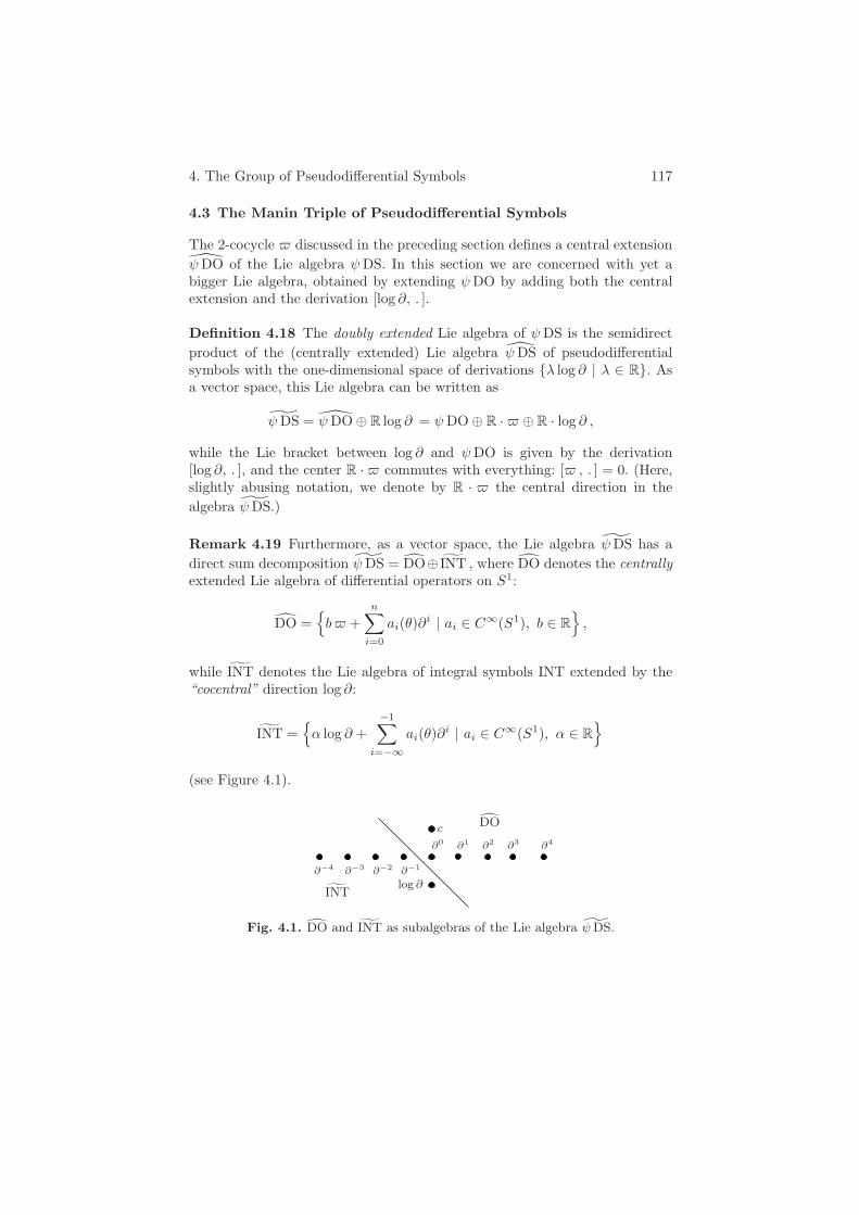
4. The Group of Pseudodifferential Symbols 117
4.3 The Manin Triple of Pseudodifferential Symbols
The 2-cocycle discussed in the preceding section defines a central extensionψDO of the Lie algebra ψDS. In this section we are concerned with yet abigger Lie algebra, obtained by extending ψDO by adding both the centralextension and the derivation [log ∂, . ].
Definition 4.18 The doubly extended Lie algebra of ψDS is the semidirectproduct of the (centrally extended) Lie algebra ψDS of pseudodifferentialsymbols with the one-dimensional space of derivations λ log ∂ | λ ∈ R. Asa vector space, this Lie algebra can be written as
ψDS = ψDO ⊕ R log ∂ = ψDO ⊕ R · ⊕ R · log ∂ ,
while the Lie bracket between log ∂ and ψDO is given by the derivation[log ∂, . ], and the center R · commutes with everything: [ , . ] = 0. (Here,slightly abusing notation, we denote by R · the central direction in thealgebra ψDS.)
Remark 4.19 Furthermore, as a vector space, the Lie algebra ψDS has adirect sum decomposition ψDS = DO⊕ ˜INT , where DO denotes the centrallyextended Lie algebra of differential operators on S1:
DO =
b +n∑
i=0
ai(θ)∂i | ai ∈ C∞(S1), b ∈ R
,
while ˜INT denotes the Lie algebra of integral symbols INT extended by the“cocentral” direction log ∂:
˜INT =
α log ∂ +−1∑
i=−∞ai(θ)∂i | ai ∈ C∞(S1), α ∈ R
(see Figure 4.1).
log ∂
c
∂0 ∂1 ∂2 ∂3 ∂4
˜INT
DO
∂−1∂−2∂−3∂−4
Fig. 4.1. DO and ˜INT as subalgebras of the Lie algebra ψ DS.

118 II. Infinite-Dimensional Lie Groups
The advantage of the double extension ψDS is that this Lie algebra admitsa nondegenerate invariant bilinear form (the “Killing form”):
Exercise 4.20 Check that the bilinear form 〈 , 〉 on the Lie algebra ψDSgiven by
〈A1+b1·+α1·log ∂ , A2+b2·+α2·log ∂〉 := tr(A1A2)+b1α2+b2α1 (4.37)
is nondegenerate and invariant. Show that the subalgebras DO and ˜INT areisotropic subspaces of ψDS with respect to this form.
Corollary 4.21 The bilinear form 〈 , 〉 on ψDS identifies the subalgebra ˜INTwith the (smooth part of) the dual to the subalgebra DO and vice versa.
These observations can be summarized in the language of Manin triples.
Definition 4.22 Three Lie algebras g, g+, and g− form a Manin triple if thefollowing two conditions are satisfied:
1. The Lie algebras g± are Lie subalgebras of g such that g = g+ ⊕ g− asvector spaces.
2. There exists a nondegenerate invariant bilinear form on g such that g+
and g− are isotropic subspaces.
Example 4.23 (i) The algebras (ψDS,DO, INT) form a Manin triple withrespect to the bilinear form 〈A , B〉 = tr(A B); cf. Exercise 4.6.
(ii) The algebras (ψDS,DO, ˜INT) form a Manin triple with respect to thebilinear form (4.37), as Exercise 4.20 shows.
The importance of Manin triples comes from the fact that there is a one-to-one correspondence between Manin triples and Lie bialgebras:
Definition 4.24 A Lie algebra g is called a Lie bialgebra if its dual spaceg∗ comes equipped with a Lie algebra structure [ , ]∗ such that the mapα : g → g ∧ g dual to the commutator map [ , ]∗ : g∗ ∧ g∗ → g∗ satisfies
adX α(Y ) = α([X,Y ]) . (4.38)
Here ad denotes the adjoint action adX(Z∧W ) = adX(Z)∧W +Z∧adX(W )of g on g ∧ g.
The condition on the map α : g → g ∧ g can be stated in terms of Liealgebra cohomology: the map α has to be a Lie algebra 1-cocycle on g relativeto the adjoint representation of g on g ∧ g.

4. The Group of Pseudodifferential Symbols 119
Theorem 4.25 Let (g, g+, g−) be a Manin triple. Then the Lie algebra g−is naturally identified with g∗+ and it endows g+ with the structure of a Liebialgebra. On the other hand, for any Lie bialgebra g there is a natural Liealgebra structure on g = g ⊕ g∗ such that (g, g, g∗) is a Manin triple.
Namely, given a Lie bialgebra g, one can define a commutator on g = g⊕g∗
by
[X +A, Y +B]g = [X,Y ]g − ad∗B(X)+ad∗
A(Y )+ [A,B]g∗ +ad∗X(B)− ad∗
Y (A)
for all X,Y ∈ g and A,B ∈ g∗. The condition that this commutator satisfythe Jacobi identity is equivalent to the condition (4.38) on the map α. For afull proof of Theorem 4.25, see, e.g., [349, 242].
Summarizing the discussion above we come to the following result.
Corollary 4.26 (= 4.21′) The Lie algebras ψDS, DO, and ˜INT form aManin triple. In particular, ˜INT is a Lie bialgebra.
Although the above correspondence of Manin triples and Lie bialgebras, aswell as the relation to Poisson Lie groups discussed below, is proved in a finite-dimensional context only, the related explicit formulas for the commutators,products, pairings, etc. work in many specific infinite-dimensional situations.In particular, they can be checked directly for the case of pseudodifferentialsymbols.
4.4 The Lie Group of α-Pseudodifferential Symbols
The Lie algebra of vector fields is the Lie algebra of a Lie group, the groupof diffeomorphisms. However, when we pass from vector fields to differentialoperators of all degrees, there is no natural Lie group attached to the corre-sponding Lie algebra DO or to its central extension DO.12
Interestingly, the Lie algebra ˜INT of integral symbols, which is dual to DOin the the Manin triple (ψDS,DO, ˜INT), comes with a group attached to it.Below we describe this group of α-pseudodifferential symbols ˜GINT.
Definition 4.27 Define the group of α-pseudodifferential symbols to be theset of monic (i.e., with the highest coefficient equal to 1) pseudodifferentialsymbols of degree α ∈ R:
˜GINT =
∂α
(
1 +−1∑
i=−∞ai(θ)∂i
)
| α ∈ R, ai ∈ C∞(S1)
.
12 One can show, for instance, that the would-be group adjoint orbits in DO aredense, which is impossible for any reasonable definition of a (smooth) groupaction.

120 II. Infinite-Dimensional Lie Groups
The group multiplication in ˜GINT is defined by equation (4.34):
∂α f = f∂α +∞∑
i=1
(
αi
)
f (i)∂α−i .
Exercise 4.28 Check that ˜GINT is indeed a group, i.e., that it is closed undertaking products and inverses.
Remark 4.29 The group ˜GINT is a semidirect product
˜GINT = GINT ∂α | α ∈ R ,
where
GINT =
1 +−1∑
i=−∞ai(θ)∂i
⊂ ˜GINT
denotes the group of monic pseudodifferential symbols of degree 0, while∂α | α ∈ R is the abelian one-parameter group of “fractional differenti-ations”: ∂α ∂β = ∂α+β , which acts on GINT.
˜GINT
˜INT
α = const
GINT
∂α
DO = ˜INT∗
log ∂
Fig. 4.2. The group ˜GINT of α-pseudodifferential symbols and its Lie algebra ˜INT.
To identify the Lie algebra for the group ˜GINT, first we consider the finite-dimensional example of the unipotent Lie group of upper triangular matri-ces with 1’s on the diagonal. Its Lie algebra is nilpotent and represented bystrictly upper triangular matrices. Similarly, we expect the Lie algebra of thegroup GINT to be given by the Lie algebra INT of integral symbols. On theother hand, we already know the Lie algebra of the one-parameter subgroup∂α | α ∈ R ⊂ ˜GINT, since it is given by R log ∂ by our construction. Thus we

4. The Group of Pseudodifferential Symbols 121
expect the group ˜GINT to have the Lie algebra ˜INT = INT α log ∂ | α ∈ R(see Figure 4.2). The following theorem formalizes this argument.
Theorem 4.30 ([198]) The exponential map exp : ˜INT → ˜GINT is well de-fined and bijective.
The bijective property of the exponential map exp : ˜INT → ˜GINT meansthat the group ˜GINT is quasi-unipotent, i.e. it is an infinite-dimensional ana-logue of the finite-dimensional unipotent group.
Remark 4.31 The idea of the proof of Theorem 4.30 is as follows. Assumethe existence of the exponential map on this group. Then for an integralsymbol A ∈ INT, the one-parameter family Ls = exp(s(a log ∂ + A)) should(by definition) satisfy the equation
(
d
dsLs
)
L−1s = a log ∂ +A (4.39)
with the initial condition L0 = 1. Equation (4.39) gives a system of differ-ential equations on the (s-dependent) coefficients of Ls, which turns out tobe uniquely solvable. Hence equation (4.39) can be used to define the one-parameter subgroup Ls and therefore the exponential map. Now the proofof Theorem 4.30 follows from the following two exercises and the Campbell–Hausdorff formula; see details in the next section.
Exercise 4.32 Show that the formula
exp(P ) =∑
k≥0
1k!P k
for an integral symbol P ∈ INT gives a well-defined map INT → GINT: thecoefficient at each ∂j in the right-hand side is a finite sum. Similarly, showthat the inverse map GINT → INT given by
log(1 + P ) =∑
k≥1
(−1)k
kP k+1
is well defined. (Hint: use the fact that degP k ≤ −k.)
The above exercise proves the following proposition, which is a “restricted”version of Theorem 4.30, by giving the explicit formula for the exponentialmap and its inverse.
Proposition 4.33 The map exp : INT → GINT is well defined and bijective.
The next exercise makes sense of the formal calculation ddα |α=0 ∂
α = log ∂we made before.

122 II. Infinite-Dimensional Lie Groups
Exercise 4.34 Verify that the element log ∂ in the Lie algebra ˜INT generatesthe one-parameter subgroup ∂α | α ∈ R ⊂ ˜GINT by computing the limitof the commutation relations of the tangent elements to the subgroups ∂αand GINT:
∂ε exp(δP ) ∂−ε exp(−δP ) = 1 + δε[log ∂, P ] + O(ε2, δ2)
for any P ∈ INT and as ε, δ → 0.
(Hint: By using the approximation exp(δP ) = 1 + δP + O(δ2) show thatthe left-hand side, modulo the terms O(δ2), is equal to
1 + δ [∂ε, P ] ∂−ε = 1 + δ∞∑
k=1
(
εk
)
a(k)j ∂j−k
for a symbol P = aj(θ)∂j . Then employ the identity ddε |ε=0
(
εk
)
= (−1)k+1
k
and the definition of log ∂.)
Remark 4.35 Note that ˜GINT is a Frechet Lie group. Indeed, the decom-position ˜GINT = GINT ∂α | α ∈ R can be used to define a topology onthis group as follows. The group GINT is the inverse limit of Frechet vectorspaces (each one being the direct sum of finitely many C∞(S1)’s, the spaces ofthe first n coefficients of the integral symbols, with the usual C∞ topology).Hence it can be endowed with the inverse limit topology. Then we equip ˜GINT
with the direct product topology of GINT and the usual topology on R in theα-direction.
4.5 The Exponential Map for Pseudodifferential Symbols
In this section we prove Theorem 4.30 on the surjectivity of the exponentialmap exp : ˜INT → ˜GINT on pseudodifferential symbols.
If P is an element in a Lie algebra (think of a matrix Lie algebra, for in-stance), the would-be exponential Ls := exp(sP ) should satisfy the differentialequation
dLs
ds (Ls)−1 = P . (4.40)
We are going to use this equation to define the element exp(P ) ∈ ˜GINT.
Lemma 4.36 For an integral symbol P , the map P → (Ls)s=1 gives a well-defined map exp : INT → GINT.

4. The Group of Pseudodifferential Symbols 123
Although this lemma is covered by Proposition 4.33, we prove it in a waythat can be easily adapted to the extended group ˜GINT below.
Proof. Fix an integral symbol P =∑−1
i=−∞ ai(θ)∂i ∈ INT . Its would-beexponent
Ls = 1 +−1∑
k=−∞uk(θ; s)∂k
has to satisfy the the differential equation (4.40) or, equivalently, ddsLs =
P Ls . Rewriting the latter equation in terms of the coefficients at ∂k fork ≤ −1, we obtain an infinite system of differential equations in the “triangularform”
d
dsuk(θ; s) = Φk (u1(θ; s), . . . , uk−1(θ; s)) . (4.41)
Here Φk is a polynomial in the u1, . . . , uk−1 and their derivatives with coeffi-cients in C∞(S1). (For example, we have d
dsu1(θ; s) = a1(θ) and ddsu2(θ; s) =
a2(θ)+a1(θ)u1(θ; s)+a1(θ)u′1(θ; s), where u′1 := ∂u1/∂θ, etc.) This system canbe solved uniquely after fixing the initial condition u(θ; 0) = 0, i.e., L0 = 1.Furthermore, since the functions ai are periodic in θ, so will be the functionsuk. Hence the exponential map is well defined for all P ∈ INT.
Now we are ready to prove
Theorem 4.30. The map exp : ˜INT → ˜GINT is well defined and bijective.
Proof. Take an element P = λ log ∂+P ∈ ˜INT, where P =∑−1
i=−∞ ai(θ)∂i
is an integral symbol from INT. Without loss of generality we set λ = 1. (Thecase λ = 0 is covered by Proposition 4.33.) Equation (4.40) now becomes
dLs
ds= (log ∂ + P ) Ls . (4.42)
Let us set Ls = (1 + Qs)∂s ∈ ˜GINT. Then the equation above assumes theform
dQs
ds= [log ∂,Qs] + P (1 +Qs) . (4.43)
Indeed, for the product Ls+εL−1s we have, after some transformations,
Ls+εL−1s = (∂ε(1 +Qs+ε) − [∂ε, Qs+ε]) (1 +Qs)−1
= 1 + ε log ∂ + εdQs
ds(1 +Qs)−1 − ε[log ∂,Qs](1 +Qs)−1 + O(ε2) ,
as ε → 0. On the other hand, this product is equal to 1+ε(
dds Ls
)
L−1s +O(ε2),
which leads to the equivalence of equations (4.42) and (4.43).Equation (4.43) gives rise to a triangular system of ordinary differential
equations similar to (4.41). Such a system can be solved uniquely, so that theexponential map is well defined on the whole Lie algebra ˜INT.

124 II. Infinite-Dimensional Lie Groups
Finally, we have to check that the exponential map is bijective. To do thiswe construct an inverse map to exp. Fix some L ∈ ˜GINT, where L = (1+Q)∂s
for an integral symbol Q =∑−1
i=−∞ ai(θ)∂i. Surjectivity of the exponentialmap INT → GINT for the nonextended group (Proposition 4.33) allows us tofind some P ∈ INT such that exp(P ) = 1 +Q. Hence we get
L = (1 +Q)∂s = exp(P ) exp(s log ∂) .
The Campbell–Hausdorff formula implies that
L = exp(P + s log ∂ + s[P, log ∂]/2 + · · · ) .
So we can define the inverse of the exponential map by
log(L) := P + s log ∂ + s[P, log ∂]/2 + · · · .
Note that each coefficient at every ∂k in the expression for log(L) is a finitesum (since the terms in the sum above have decreasing degree due to theincreasing number of commutators). Therefore, the map log : ˜GINT → ˜INTis well defined, which implies that the exponential map exp : ˜INT → ˜GINT isindeed bijective.
4.6 Poisson Structures on the Group of α-PseudodifferentialSymbols
The fact that the Lie algebra ˜INT of integral symbols is actually a Lie bial-gebra (or a part of a Manin triple) implies that the corresponding Lie group˜GINT is a Poisson Lie group:
Definition 4.37 A Poisson Lie group (G, , ) is a Lie group G equippedwith a Poisson structure , such that the multiplication G × G → G andthe inverse mapping G → G− (sending g → g−1) are Poisson maps, whereG×G carries the product Poisson structure and G− denotes the Lie group Gequipped with the opposite Poisson structure − , .
Theorem 4.38 For any connected and simply connected Lie group G, thereis a one-to-one correspondence between Lie bialgebra structures on its Liealgebra g and Poisson Lie group structures on G.
For a proof of this theorem, see, e.g., [349, 242]. The explicit constructionof the Poisson bracket on G from the Lie bialgebra structure on g is as follows.Regard the Lie bialgebra g as a part g = g− of the Manin triple (g, g+, g−)with corresponding Lie groups G, G+, and G−. (We write g+ = g∗ and g− = g
in order to distuinguish between the different duals involved.) Define the fol-lowing Poisson structure on the group G = G−. Let ξ, η ∈ T ∗
g G− be cotangent
4. The Group of Pseudodifferential Symbols 125
vectors to G− at a point g ∈ G− and let ξ, η be arbitrary extensions of ξ andη to cotangent vectors of the group G ⊃ G− at g. Furthermore, denote by r∗g ξ
and l∗g ξ the pullbacks of ξ ∈ T ∗g G to T ∗
e G = g∗ via, respectively, the right andleft translations. Finally, let ( )+ be the projection of g∗ to g∗+ = g− along g∗−and define ( )− analogously. Then the Poisson structure on the group G = G−is defined by the bivector field Π whose value on the covectors ξ and η at thepoint g is given by the following formula:
Πg(ξ, η) = 〈(r∗g ξ)+, r∗g η〉 − 〈(l∗g ξ)+, l∗g η〉 . (4.44)
Remark 4.39 Note that we do not actually need the existence of Lie groupsG and G+ corresponding to the Lie algebras g and g+. For the above con-struction to work, it suffices to know how the Lie group G− acts on the bigLie algebra g = g+⊕g−. Indeed, for cotangent vectors ξ, η ∈ T ∗
g G− at a pointg ∈ G, let A = r∗gξ and B = r∗gη denote their pullbacks to T ∗
e G− = g∗−. Now,if A and B are any liftings of A,B ∈ g∗− = g/g∗+ to g, then formula (4.44) forthe Poisson structure on the group G− can be rewritten in the form
Πg(ξ, η) = 〈(A)+, B〉 − 〈(Ad∗g A)+,Ad∗
g B〉 . (4.45)
This observation allows one to extend this construction to the infinite-dimensional case at hand. Indeed, set g− = ˜INT and g+ = DO, while thegroup ˜GINT acts on the Lie algebra ψDS by conjugation. Then formula (4.45)defines a bivector field on the group ˜GINT, which endows it with the structureof a Poisson Lie group.
Corollary 4.40 The group ˜GINT carries a natural Poisson structure thatgives it the structure of a Poisson Lie group.
Our next goal will be to identify this Poisson structure on the group ˜GINT
explicitly. Let us express ˜GINT =⋃
α∈R˜Gα as a union of the “hyperplanes”
˜Gα =
L | L = ∂α (
1 +−1∑
k=−∞uk(z)∂k
)
of symbols of fixed degree α = const.
Definition 4.41 The quadratic (or second) generalized Gelfand–DickeyPoisson structure , GD on the group ˜GINT is defined as follows:
1. The degree function α is its Casimir function, i.e., the hyperplanes ˜Gα arePoisson submanifolds for this Poisson structure. In other words, for twofunctions f, g : ˜GINT → R, the value of their Poisson bracket f, gGD atany point L = ∂α0(1 + · · · ) ∈ ˜GINT depends only on the restriction of fand g to the hyperplane ˜Gα0 .
126 II. Infinite-Dimensional Lie Groups
2. The subsets ˜Gα are affine spaces, so one can identify the tangent space tothe hyperplane ˜Gα0 of symbols of fixed degree α0 with the set ∂α0 INT:a tangent vector at the symbol L of degree α0 has the form δL = ∂α0 ∑−1
k=−∞ uk(z)∂k ∈ ∂α0 INT.This allows one to identify the corresponding cotangent space withDO ∂−α0 . Any cotangent vector A ∈ DO ∂−α0 defines a linear func-tional FA on the tangent space ∂α0 INT via the following pairing:
FA(δL) := 〈A, δL〉 = tr(A δL) .
Here the product A δL is a symbol of integral degree and its trace tr iswell defined.
3. Finally, it is sufficient to define the Poisson bracket on linear functionals,and
FA, FBGD(L) := FB (VA(L)) ,
where VA is the following Hamiltonian mapping FA → VA(L) (from thecotangent space A to the tangent space δL):
VA(L) = (L A)+ L− L (A L)+ . (4.46)
Here X+ denotes the purely differential part of a pseudodifferential symbolX ∈ ψDS.
Note that in the above formula for the Poisson bracket we regard thefunctional FB as a linear functional on the space ˜Gα0 in the left-hand side,and as a covector (on the tangent space) at L in the right-hand side. Thebracket of two functionals linear in L may already be quadratic in L.
Exercise 4.42 Show that VA(L) is well defined as a vector field on ˜Gα0 , i.e.,show that deg VA(L) ≤ α0 − 1 and its degree differs from α0 by an integer.(Hint: one can rewrite VA(L) in the form
VA(L) = (L A− (L A)−) L− L (A L− (A L)−)= −(L A)− L+ L (A L)− ,
where X− = X −X+ stands for the purely integral part of a symbol X.)
Theorem 4.43 ([198, 101]) The Poisson structure of the Poisson Lie group˜GINT coincides with the quadratic generalized Gelfand–Dickey structure.
We start with the following lemma:
Lemma 4.44 The function deg : ˜GINT → R, which assigns to a pseudodif-ferential symbol its degree, is a Casimir function on ˜GINT, i.e., it Poisson-commutes with all differentiable functions on ˜GINT.

4. The Group of Pseudodifferential Symbols 127
Proof. First observe that the pullback of the differential ddeg from anypoint L to the identity in ˜GINT corresponds to the covector A = (0, 1) ∈ DO =DO⊕R ·, which is an element of the center of the Lie algebra DO. Extend A
to an element A = (0, 1, 0) in the center of ψDS = ψDS⊕R·⊕R·log ∂. (Here,0 denotes the extension of 0 ∈ DO to the zero element in ψDS = DO⊕ INT.)Now one can see that the expression
〈(0, 1, 0)+, (B, b, β)〉 − 〈(L−1 (0, 1, 0) L)+, L−1 (B, b, β) L〉
from equation (4.45) vanishes for all (B, b, β) ∈ ψDS. Hence, the function degis indeed a Casimir function on ˜GINT.
Proof of Theorem 4.43. Lemma 4.44 implies that the hyperplanesdeg(L) = const in ˜GINT are Poisson submanifolds, and we can restrict ourattention to their tangent spaces. Let X and Y be cotangent vectors at L tothe hyperplane α = α0. Regard X and Y as elements of DO ∂−α0 . Let X andY denote arbitrary extensions of X and Y to ψDS ∂−α0 . By the definitionof the Poisson bracket on ˜GINT, one can write
ΠL(X,Y ) =〈(r∗LX)+, r∗LY 〉 − 〈(Ad∗L(r∗LX))+,Ad∗
L r∗LY 〉
=〈(L X)+, L Y 〉 − 〈(X L)+, Y L〉=〈(L X)+ L− L (X L)+, Y 〉 ,
which is the quadratic generalized Gelfand–Dickey bracket. (In the calculationabove, we used that right multiplication on vectors becomes left multiplicationon covectors.)
INT ∂α
INT
∂0
˜GINT
GINT
α = const∂α
Fig. 4.3. The tangent space to the hyperplane α = const in the group ˜GINT.
Definition 4.45 The linear (or first) generalized Gelfand–Dickey structurecan be defined on the “integral” hyperplanes ˜Gα with α ∈ Z in the group˜GINT by setting

128 II. Infinite-Dimensional Lie Groups
V 1A(L) := [L,A]+ − [L,A+] . (4.47)
Proposition 4.46 The first and the second generalized Gelfand–Dickeystructures are compatible.
Proof. Indeed, from formula (4.46) for VA(L) we obtain
VA(L+ λ∂0) = VA(L) + λV 1A(L) ,
so that VA(L) + λV 1A(L) is the second Gelfand–Dickey structure shifted by
λ∂0. Note that the shift of L by λ∂0 makes sense only if L is of integraldegree.
Remark 4.47 The classical definitions of both the first and the secondGelfand–Dickey (also called Adler–Gelfand–Dickey) structures are usuallygiven in the case that α is a fixed positive integer n and L is a differentialoperator; cf. [3, 80].
One can see that for the second (quadratic) bracket, the set Ln := L ∈˜Gn | L+ = L of purely differential operators is a Poisson submanifold in thePoisson “hyperplane” ˜Gn of all monic pseudodifferential symbols of the samedegree n. Indeed, for any differential operator L = ∂n + un−1∂
n−1 + · · · +u0 and an arbitrary symbol A from the space DO ∂−n, the correspondingHamiltonian vector VA(L) = (LA)+ L − L(AL)+ is always a differentialoperator of order n−1, and hence all Hamiltonian fields keep the submanifoldLn of such differential operators invariant.
The corresponding quadratic Poisson algebras of functions on the sets Ln
(or, more generally, on the hyperplanes deg(L) = n) are also called classicalWn-algebras.
Exercise 4.48 Show that in the Poisson Lie group ˜GINT not only are thesubmanifolds Ln of purely differential operators Poisson, but so are the sub-manifolds L−1
n of the inverses of differential operators, as well as the productsL−1
n Lm for any n and m. (Hint: use the properties of a Poisson Lie group thattaking products and inverses are Poisson maps.)
Remark 4.49 Another point to mention is that the linear Gelfand–Dickeybracket simplifies significantly when it is restricted to purely differential oper-ators. Namely, linear functionals on the spaces Ln are given by pseudodifferen-tial symbols A of degree deg(A) ≤ −1 via the pairing 〈A,L〉 = tr(AL). Sincethe degree of A is negative, we have A+ = 0, whence the term [L,A+] doesnot appear in the expression for V 1
A(L) above. Thus in this case, the first gen-eralized Gelfand–Dickey structure reduces to the usual first Gelfand–Dickeystructure defined as V1
A(L) := [L,A]+. Finally, note that the latter Poissonstructure is nothing else but the linear Lie–Poisson structure on differential
4. The Group of Pseudodifferential Symbols 129
operators, regarded as the dual space DO = INT∗ to the Lie algebra INT ofintegral symbols [234].
Remark 4.50 Both the first and the second Gelfand–Dickey Poisson struc-tures on the spaces Ln can also be obtained by a Hamiltonian reduction fromthe dual of the affine Lgl(n)-algebras in the classical Drinfeld–Sokolov re-
duction. The linear Lie–Poisson structure on Lgl(n)∗
becomes the quadraticGelfand–Dickey bracket on Ln after the reduction, while a constant Poissonstructure on Lgl(n)
∗becomes the linear Gelfand–Dickey bracket. We describe
this construction in Appendix A.8.It turns out that this reduction procedure can be extended to the whole
hyperplanes deg(L) = α and can also be defined for an arbitrary complexdegree α; see [191]. The corresponding affine algebra before the reduction isconstructed with the help of the algebra gl(α) for any complex α (“the algebraof matrices of complex size”) introduced in [116].
4.7 Integrable Hierarchies on the Poisson Lie Group ˜GINT
Consider the following family of Hamiltonian functions Hm : ˜GINT → R
parametrized by an integer parameter m ∈ N: the value of Hm at thepseudodifferential symbol L ∈ ˜GINT of degree α = 0 is
Hm(L) :=α
mtr(Lm/α) .
Here any real power of L is a uniquely defined element in ˜GINT, since the group˜GINT is quasi-unipotent and the exponential map is one-to-one; see Theorem4.30 and Section 4.5. One can think of the powers Lm/α as intersections ofthe one-parameter subgroup Lt passing through L with the “hyperplanes” ofsymbols of integral degree m. Since deg(L) = α, the degree deg(Lm/α) = mis an integer, and hence both the corresponding trace tr and the function Hm
are well defined.
Theorem 4.51 ([198, 101]) 1. The Hamiltonian equations correspondingto the functions Hm are well defined on any hyperplane deg(L) = const =0 in the Poisson Lie group ˜GINT.
2. Each function Hm defines the following Hamiltonian equation with respectto the (quadratic) Poisson structure on ˜GINT:
∂L
∂tm= [(Lm/α)+, L] , (4.48)
where (Lm/α)+ denotes the purely differential part of the symbol Lm/α.3. All the functions Hm, m = 1, 2, . . . , are first integrals for each of these
Hamiltonian equations. Equivalently, these functions Hm are pairwise ininvolution with respect to the Poisson structure on the group ˜GINT.

130 II. Infinite-Dimensional Lie Groups
Proof. (1) The flows of the Hamiltonians Hm do not change the degree ofsymbols, since deg(L) is a Casimir function on ˜GINT.
(2) We prove part 2 for α = 1 (and refer to [198, 101] and the exercisebelow for general α). In this case, deg(L) = 1 and Hm(L) = 1
m tr(Lm). Towrite out the Hamiltonian equations we need to find the variational derivativeδHm/δL of the Hamiltonian function first. By definition,
⟨δHm
δL(L), δL
⟩
:=d
dε
∣
∣
∣
ε=0Hm(L+ ε · δL)
= limε→0
1ε
(
1m
tr((L+ ε · δL)m) − 1m
tr(Lm))
= tr(Lm−1δL) .
Recall that tangent vectors δL to the set of symbols L | deg(L) = 1 aresymbols of degree 0. Then the cotangent vectors to the same set have the formDO ∂−1. In particular, we have δHm/δL = (Lm−1)≥−1, i.e., the variationalderivative δHm/δL is the part of the symbol Lm−1 in which we keep onlythe terms of degree ≥ −1. We can, however, use the whole symbol Lm−1 asthe variational derivative δHm/δL, since other terms do not contribute to thepairing 〈A, δL〉 = tr(A δL) between the tangent and cotangent spaces.
Now substitute the value δHm/δL = Lm−1 to the definition of theGelfand–Dickey bracket to find the corresponding Hamiltonian field:
VδHm/δL(L) = (L Lm−1)+ L− L (Lm−1 L)+= (Lm)+ L− L (Lm)+ = [(Lm)+, L] .
This implies the form of the Hamiltonian equations given in the theorem. Thecase of general α is handled similarly by showing that δHm/δL = L(m/α)−1,but requires a bit more work (see below).
(3) The last part now follows directly, since the flow for Hm changes asymbol into a conjugate one. Thus, the ad-invariant function Hn stays invari-ant on the flow lines of Hm, so that the commutator Hm,Hn vanishes forall m,n.
Exercise 4.52 Verify the last statement of the theorem above directly byobtaining zero as a result of the differentiation:
Hm,Hn =∂Hn
∂tm=
α
n
∂ tr(Ln/α)∂tm
.
Exercise 4.53 Prove that for general α = 0 one has δHm/δL = L(m/α)−1.(Hint: first prove this for integral values of α; then use that the coefficients ofboth sides depend rationally on α; see details in [198, 101].)

4. The Group of Pseudodifferential Symbols 131
Exercise 4.54 Prove that the first flow at any hierarchy has the form
∂L
∂t1=
∂L
∂θ,
which expresses the fact that the space variable θ can be taken as the firsttime variable.
Remark 4.55 Equations (4.48) form an infinite sequence of commuting flowson the coefficients of the symbols L. These flows are defined on the hyperplanesof symbols of fixed degree α and are universal in the sense that they interpolatebetween several well-known hierarchies of integrable Hamiltonian systems.Here we list a few interesting cases; cf. [372]:
1. On the hyperplane deg(L) = 1 one obtains the so called Kadomtsev–Petviashvili (KP) hierarchy, which has two equivalent and commonly usedwritten forms:
∂L
∂tm= [(Lm)+, L] = −[(Lm)−, L] .
The compatibility (or zero curvature) equation between the second andthe third flows of this hierarchy,
∂(L2)+∂t3
− ∂(L3)+∂t2
= [(L3)+, (L2)+] , (4.49)
leads to the Kadomtsev–Petviashvili equation in the form
(4ut3 − 12uuθ − uθθθ)θ − 3ut2t2 = 0 (4.50)
on the function u(θ, t2, t3) of two space variables θ = t1 and t2 and onetime variable t3 (see also Exercise 4.56 below). The latter is often regardedas a two-dimensional version of the KdV equation: the KdV solutions giverise to the KP solutions independent of the space variable t2.
2. The restriction of the universal hierarchy to the Poisson submanifoldsLn := L | L+ = L , deg(L) = n of purely differential operators ofdegree n gives the n-KdV hierarchy
∂L
∂tm= [(Lm/n)+, L] , m = 1, 2, . . . , n− 1, n+ 1, n+ 2, . . . .
The classical KdV hierarchy corresponds to the case n = 2 and L =∂2+u(θ). (Notice the familiar form of a Hill’s operator.) The KdV equationappears for m = 3 as an evolution equation on the potential u(θ).Another classical case is the Boussinesq equation, which corresponds ton = 3, m = 2 and arises as a pair of equations on two functions u, v inthe variables θ, t:
uθθ − 2vθ + ut = 0 ,2uθθθ − 3vθθ + 3vt + 2uuθ = 0 .
132 II. Infinite-Dimensional Lie Groups
Using cross differentiation, it is possible to eliminate v and obtain theequation
3utt + uθθθθ + 2(u2)θθ = 0 . (4.51)
3. Consider the space Kn,m := L−1n Lm of rational pseudodifferential symbols
on the circle, i.e., the space of symbols of the form L−11 L2, where L1 and
L2 are (mutually prime) monic differential operators of degree n and mrespectively. As we discussed in the preceding section, such spaces arePoisson submanifolds, and one can restrict to them the Hamiltonian flows.The restriction of the universal hierarchy to these spaces generates therational reductions of the KP hierarchy [217].
4. Consider also pseudodifferential symbols with complex coefficients andtake the Hamiltonians Hm(L) = i
m tr(Lm). Then for m = 2 and L =∂ +ψ∗∂−1ψ, the corresponding Hamiltonian flow generates the nonlinearSchrodinger equation (NLS) in the form
i∂ψ
∂t= ψθθ + 2|ψ|2ψ .
This equation can also be viewed as a rational KP reduction to the sub-manifold K1,2; see details in [217].
Exercise 4.56 Show that the compatibility equation (4.49) for a symbol L =∂ + u∂−1 + v∂−2 + · · · yields the following system of equations for u and v:
ut2 =uθθ + 2vθ ,
3vt2 + 3uθt2 + 6uuθ = 3vθθ + 2ut3 + uθθθ .
Use cross differentiation to eliminate v from the equations above and obtainthe Kadomtsev–Petviashvili equation (4.50) for u.
4.8 Bibliographical Notes
Various structures related to pseudodifferential symbols are described in detailin the book [80]. The Adler–Gelfand–Dickey brackets were defined in [3, 142].The Poisson Lie group approach to these structures was presented in [101,198], where we refer the interested reader for more details on the questionsdiscussed in this section. The reader can find a brief introduction to PoissonLie groups in [87, 242, 349], for example.
The Adler–Gelfand–Dickey structures on scalar differential operators canbe obtained via the Drinfeld–Sokolov reduction from matrix operators; see[88, 115] and Appendix A.8. This reduction extends to the symbols of allcomplex degrees [192]. In the mathematical physics literature, the Gelfand–Dickey Poisson algebras are called classical W -algebras; see [112, 41, 81]. TheLie algebra and Poisson Lie group of pseudodifferential symbols have naturalq-analogues, which were described in [313, 314]; see also [131].
4. The Group of Pseudodifferential Symbols 133
The 2-cocycle on differential operators on the circle appeared in [179],while the logarithmic 2-cocycle on the Lie algebra of pseudodifferential sym-bols on the circle was introduced in [215]. For generalizations of the loga-rithmic cocycle to symbols on higher-dimensional manifolds see [324, 94]. Forthe description of cohomology of Lie algebras of differential operators andpseudodifferential symbols see [116, 118, 94]. Representations of the centrallyextended Lie algebra of differential operators were studied in [180, 130]. Thelogarithmic cocycle also appears in the study of the multiplicative anomalyfor determinants of elliptic pseudodifferential operators [211].
One can find in [372, 250, 129] more details on the corresponding equa-tions of mathematical physics. For rational reductions of the KP hierarchy werefer to [217, 102, 186], while higher-dimensional extensions of this hierarchyare described in [310]. Quantum versions of the corresponding equations arediscussed, for example, in [117].

134 II. Infinite-Dimensional Lie Groups
5 Double Loop and Elliptic Lie Groups
While loop algebras have the one-dimensional central extension, current alge-bras on compact manifolds admit infinite-dimensional central extensions oncethe manifold dimension is bigger than 1. However, if the manifold M is a two-dimensional (Riemann) surface regarded as a complex curve, there is a wayto choose a special and, in many respects, natural finite-dimensional centralextension for the current algebra on M . While the nonextended algebra itselfis the same for all choices of the complex structure, it is the 2-cocycle on thiscurrent algebra that relies on this choice.
In this section we consider the case of an elliptic curve M = Σ, wherethe theory is most complete. The corresponding Lie algebra is often calledthe double loop or elliptic Lie algebra. It turns out that many constructionsfor the affine algebras have their analogues for the elliptic case. In particular,the coadjoint orbits of the corresponding elliptic Lie group are classified byequivalence classes of holomorphic G-bundles over the elliptic curve.
It turns out that the Calogero–Moser dynamical systems provide a bridge,or, rather, a ladder that unites the three classes of the Lie algebras: there is auniversal construction of a Hamiltonian reduction on the dual of a Lie algebra,which for the finite-dimensional simple Lie algebras, affine Lie algebras, andelliptic Lie algebras leads to the Calogero–Moser integrable systems with,respectively, rational, trigonometric, and elliptic potentials.
5.1 Central Extensions of Double Loop Groupsand Their Lie Algebras
Let g be a complex semisimple Lie algebra and G the corresponding simplyconnected Lie group. Throughout this section we fix an elliptic curve Σ, i.e.,a 2-dimensional torus endowed with a complex structure. One can alwaysrepresent such a curve as a quotient Σ = C/(Z + τZ), where τ is a complexnumber with Im τ > 0. Fix a holomorphic 1-form dz on Σ, which is canonicalup to a complex factor.
0 0
τ
C/(Z + τZ)
11
C/Z
Fig. 5.1. A cylinder and an elliptic curve as quotients of C.
The double loop algebra gΣ is the Lie algebra of smooth maps from thetorus Σ to the Lie algebra g with the pointwise bracket, gΣ = C∞(Σ, g). Note

5. Double Loop and Elliptic Lie Groups 135
that neither the elements nor the commutator of the double loop algebra de-pends on the complex structure on Σ. However, the complex structure entersthe definition of the central extension of gΣ .
Definition 5.1 The elliptic Lie algebra corresponding to the Lie algebra g
and the elliptic curve Σ is the complex one-dimensional central extensiongΣ of the double loop algebra gΣ defined as the vector space gΣ = gΣ ⊕ C
endowed with the following commutator:
[(X(z, z), a) , (Y (z, z), b)] =(
[X(z, z), Y (z, z)] ,∫
Σ
dz ∧ 〈X, dY 〉)
,
where 〈 , 〉 denotes the Killing form on the Lie algebra g.
By decomposing the operator d = ∂ + ∂ into its Dolbault components ∂and ∂, one can rewrite the cocycle ωΣ that defines the central extension as
ωΣ(X,Y ) :=∫
Σ
dz ∧ 〈X, ∂Y 〉 . (5.52)
Note that the complex structure of the elliptic curve Σ appears only in thecocycle ωΣ , and conformal equivalence of curves induces the isomorphism ofthe elliptic algebras.
The Lie group corresponding to the double loop algebra gΣ is given by thedouble loop group GΣ , where G is the simply connected complex Lie groupcorresponding to the Lie algebra g. Similarly to the case of the loop group, thecentral extension of the double loop algebra gives rise to an extension of thecorresponding group. However, the group extension is now given by means ofa “complex analogue of the circle.” Namely, the elliptic curve Σ itself can beregarded as such an analogue, while the identification Σ = C/(Z + τZ) givesit the structure of an abelian group.
Theorem 5.2 The central extension gΣ of the Lie algebra gΣ lifts to a centralextension GΣ of the current group GΣ, where the extension is by means ofthe elliptic curve Σ itself:
e → Σ → GΣ → GΣ → e .
The central extension GΣ , called the elliptic Lie group, can be constructedsimilarly to the central extension of the loop group LG (see [322, 106]). Moreexplicit (quotient) constructions either use ingenious generalizations [241] ofthe construction of the affine group (see [263]; cf. Section 1.3) or are purelycomplex and involve the higher-dimensional residues (see [133]; cf. ChapterIII for more details).
Remark 5.3 In a similar way one can define the current algebra for anycompact Riemann surface (or complex curve) C of genus κ > 0. Let HC =
136 II. Infinite-Dimensional Lie Groups
H0(C, Ω1C) be the vector space of holomorphic differentials on C, which has
the complex dimension dim(HC) = κ. Define a complex κ-dimensional centralextension of the Lie algebra gC by the following 2-cocycle ωC with values inH∗
C , dual to the space HC of holomorphic differentials. Namely, set the valueof this cocycle on any holomorphic 1-form α on C to be
ωC(X,Y )(α) :=∫
Cα ∧ 〈X, ∂Y 〉 .
This central extension lifts to a central extension of the current group GC =C∞(C, G), this time by the Jacobian J(C) of the complex curve C:
e → J(C) → GC → GC → e ;
see [106]. If C is an elliptic curve Σ, its Jacobian is given by the curve Σ itself,and one recovers the central extension of the double loop group describedabove.
Remark 5.4 If M is of real dimension 2, but it is not equipped with acomplex structure, or if M is higher-dimensional, then a priori, we do nothave a preferred choice of a finite-dimensional cocycle. For any compactM the universal extension of the current algebra is by means of the spaceΩ1(M)/dΩ0(M) of all 1-forms on M modulo exact 1-forms; see Remark 1.7in Chapter II. For details, the interested reader is referred to [322, 287, 288],where one can find the study of this extension for a general manifold M ,including the noncompact case and the case with boundary.
5.2 Coadjoint Orbits
In this section, we study the coadjoint representation of the elliptic Lie groupGΣ for the elliptic curve Σ.
Definition 5.5 The (smooth part of the) dual space (gΣ)∗ of the Lie algebragΣ is identified with the space gΣ ⊕ C via the pairing
〈(A, a), (X, c)〉 :=∫
Σ
〈A,X〉dz ∧ dz + a · c ,
where 〈 , 〉 is the Killing form on the finite-dimensional Lie algebra g, (X, c) ∈gΣ , and (A, a) ∈ (gΣ)∗ = gΣ ⊕ C.
Proposition 5.6 In the coadjoint representation of the elliptic Lie group GΣ
an element g ∈ GΣ acts on the dual space (gΣ)∗ as follows:
g : (A, a) → (Adg(A) + a(∂g)g−1, a) .
5. Double Loop and Elliptic Lie Groups 137
In other words, elements of the dual space (gΣ)∗ can be thought of as∂-connections −a∂ +A(z, z), while the group coadjoint action is the gaugeaction on these connections, cf. Remark 1.13.
This proposition describes the coadjoint representation of the whole groupGΣ completely, since the center acts trivially in the coadjoint representation.
Proof. The proof repeats that for the corresponding statement for the affineLie groups.
One of the main features of the centrally extended elliptic Lie algebrasand Lie groups is a nice classification of their coadjoint orbits in terms ofholomorphic principal G-bundles over the elliptic curve Σ. To study them wefirst note that the hyperplanes a = const are invariant under the coadjointaction of the group GΣ in the dual space (gΣ)∗. Fix a nonzero value of a andexamine the orbits contained in the corresponding hyperplane Ha ⊂ (gΣ)∗.
Theorem 5.7 ([106]) Coadjoint orbits of the group GΣ in the hyperplaneHa are in one-to-one correspondence with equivalence classes of holomorphicG-bundles over Σ.
Proof. Given an element (A, a) ∈ (gΣ)∗, we consider the operator D =a∂−A and associate to it a holomorphic principal G-bundle over Σ as follows.Consider the partial differential equation
a∂ψ −Aψ = 0 .
(Here one can think of A as a g-valued (0, 1)-form, the operator D = a∂−A asa partial (0, 1)-connection, while ψ is a horizontal section for this connection;cf. Section III.1.1.) One can find an open covering Ui, i ∈ I, of the curve Σsuch that there exist local solutions ψi : Ui → G of this equation. Now definetransition functions φij : Ui ∩ Uj → G by ϕij = ψ−1
i ψj . It is easy to seethat these functions are holomorphic and satisfy ϕij = ϕ−1
ji on Ui ∩ Uj andϕijϕjkϕki = id on Ui ∩ Uj ∩ Uk. Thus, they can be taken to be the gluingfunctions of a holomorphic principal G-bundle P (A) on the curve Σ.
Conversely, for any holomorphic principal G-bundle P on Σ there existsan operator D = a∂−A such that P = P (A). Indeed, any principal G-bundleon Σ is topologically trivial, since G is simply connected. When a globaltrivialization is chosen, the local holomorphic trivializations over open sets Ui
will be expressed by smooth functions ψi : Ui → G such that the transitionfunctions ϕij = ψ−1
i ψj are holomorphic on Ui ∩ Uj .Then we have
∂ψi · ψ−1i = ψj · ∂(ψ−1
j ψi) · ψ−1i − ψj · ∂ψ−1
j = ∂ψj · ψ−1j
on Ui ∩ Uj . Therefore there exists a g-valued 1-form A on Σ such that A =a∂ψi · ψ−1
i on Ui for all i ∈ I. Set D = a∂ −A. Then the bundle P is definedas the bundle P (A).

138 II. Infinite-Dimensional Lie Groups
Finally, two holomorphic principal G-bundles P (A1) and P (A2) are iso-morphic if and only if there exists some g ∈ GΣ such that A2 = gA1g
−1 +a(∂g)g−1, i.e., if the differential operators D1 = a∂ − A1 and D2 = a∂ − A2
are related by a gauge transformation: g D1 = D2.
Exercise 5.8 Define an elliptic analogue of the Virasoro algebra, i.e., a cen-tral extension of the Lie algebra Vect(0,1)(Σ) of (0, 1)-vector fields on theelliptic curve Σ and describe its coadjoint orbits. (Hint: cf. [106].)
In a similar way one can define an analogue of the Virasoro algebra for acomplex curve C of genus κ > 1, where it is going to be a central extension ofthe Lie algebra Vect(0,1)(C) of complex dimension κ; see [106]. This extensionturns out to be universal [380]. One can also define the elliptic analogues ofthe Gelfand–Dickey brackets on the space of differential operators of higherorder,
∑nk=0 uk(z, z)∂k | uk ∈ C∞(Σ,C); see [107].
Remark 5.9 For an arbitrary complex curve (i.e., a compact Riemann sur-face) C, the orbits of the group GC in the module of (0, 1)- (or ∂-) connectionshave a nice geometric interpretation similar to the one described above [106].Namely, these orbits can be classified in terms of equivalence classes of holo-morphic principal G-bundles on the complex curve C.
However, for higher-genus curves, the space of such connections is not ahyperplane in the corresponding dual space of the Lie algebra gC . (The iden-tification does not work directly, since the holomorphic differentials definingthe 2-cocycle have zeros on C.) The classification of coadjoint orbits of thecorresponding group GC for C of higher genus is still unknown.
5.3 Holomorphic Loop Groups and Monodromy
Recall that coadjoint orbits of a centrally extended loop group LG can beclassified in terms of conjugacy classes of the corresponding finite-dimensionalLie group G. Namely, the conjugacy class corresponding to a coadjoint orbitcan be interpreted as the monodromy of a (necessarily flat) connection onthe circle. As we shall see in this section, the coadjoint orbits of the centrallyextended double loop group GΣ admit a similar description.
Definition 5.10 Let HoLG denote the group of holomorphic maps from thecylinder C/Z to a simply connected complex Lie group G with pointwisemultiplication:
HoLG = g : C/Z → G | g holomorphic .
The group HoLG is called the holomorphic loop group of G.

5. Double Loop and Elliptic Lie Groups 139
Fix some τ ∈ C. We define the “τ -twisted” conjugacy classes of the groupHoLG as the orbits of the HoLG-action on itself given by
g(z) : h(z) → hg(z) := g(z)h(z)g(z + τ)−1 . (5.53)
(These orbits depend only on the coset τ + Z, and below, τ is regarded as anelement of C or C/Z whenever this does not cause ambiguity.)
Remark 5.11 The τ -twisted conjugacy classes of the group HoLG can beseen as “restricted conjugacy classes” of the bigger group HoLG = HoLG
C/Z. More precisely, the cylinder C/Z acts on the group HoLG through trans-lations of the argument (i.e., by “rotating” the loops, τ : f(z) → f(z + τ)),and we form the semidirect product HoLG = HoLG C/Z associated to thisaction. The group HoLG acts on itself by conjugation.
Exercise 5.12 For (f, t) and (g, τ) ∈ HoLG we have (f, t)(g, τ)(f, t)−1 =(h, τ), where
h(z) = f(z)g(z + t)f(z + τ)−1
for z ∈ C/Z.
One can see that this action leaves the subset HoLG × τ with fixed τ
invariant. The restricted conjugacy classes of the group HoLG are the HoLG-orbits in the “hyperplane” HoLG × τ , where HoLG is viewed as a subgroupof the larger group HoLG.
For what follows we assume that Im τ > 0. The next theorem can bethought of as a direct analogue of the corresponding theorem for ordinaryloop groups.
Proposition 5.13 Let Σ = C/(Z + τZ) be the elliptic curve with an ellipticparameter τ . For any fixed a = 0 there is a one-to-one correspondence betweencoadjoint orbits of the group GΣ in the hyperplane Ha = (A, a) | A ∈ gΣ ⊂(gΣ)∗ and τ -twisted conjugacy classes in the holomorphic loop group HoLG.
Proof. Let A be a smooth function on the torus Σ. Consider the differentialequation
a∂ψ −Aψ = 0 (5.54)
with respect to a G-valued function ψ on the cylinder C/Z.Let ψ0(z) be a solution of this equation. Then ψ0(z+ τ) is also a solution,
since the equation is periodic in τ . Therefore, ν0(z) = ψ0(z)−1ψ0(z+τ) is alsoa G-valued function on the cylinder that is holomorphic, since ∂ν0/∂z = 0. Ifwe choose another solution of equation (5.54), say, ψ1, it will have the formψ1(z) = ψ0(z)µ(z), where µ is a holomorphic G-valued function on the samecylinder. Therefore, the function ν1(z) = ψ1(z)−1ψ1(z + τ) can be expressed

140 II. Infinite-Dimensional Lie Groups
as follows: ν1(z) = µ(z)−1ν0(z)µ(z + τ). This implies that the τ -twisted con-jugacy class of the element (ν0, τ) is independent of the choice of the solutionψ0 of equation (5.54). Thus we have associated a twisted conjugacy class ofHoLG to any equation of the form (5.54).
Now we note that different equations of this form (5.54) associated todifferential operators from one coadjoint orbit give the same twisted conjugacyclass in HoLG. Indeed, fix some element g ∈ GΣ and, as before, let ψ0 denotea solution of (5.54). Then the G-valued function φ = g ·ψ0 gives a solution ofthe equation
a∂φ− (gAg−1 + a(∂g)g−1)φ = 0 .
Since g is periodic in τ , we obtain
φ(z)−1φ(z + τ) = ψ0(z)−1g(z)−1g(z + τ)ψ0(z + τ) = ψ0(z)−1ψ0(z + τ) .
This shows that the restricted conjugacy class of HoLG associated to theelement (A, a) ∈ gΣ ⊕ C with a = 0 is the same as the restricted conjugacyclass associated to the element (gAg−1 + a(∂g)g−1, a), i.e., one and the sameclass corresponds to a coadjoint orbit of the group GΣ .
It remains to show that every conjugacy class in HoLG × τ comes froma certain equation (5.54). Given an element g ∈ HoLG, we take any smoothmap ψ : C/Z → G satisfying g(z) = ψ(z)−1ψ(z + τ) and set A := a(∂ψ)ψ−1.The fact that ψ(z)−1ψ(z + τ) is holomorphic implies that A is periodic in τ ,since
0 = a∂(ψ(z)−1ψ(z + τ)) = ψ(z)−1(−A(z) +A(z + τ))ψ(z + τ) .
Therefore, A is a smooth map from the elliptic curve Σ to the Lie algebrag, while the conjugacy class corresponding to the coadjoint orbit through(A, a) ∈ gΣ ⊕ C gives the τ -twisted conjugacy class through the elementg ∈ HoLG. Thus we have established a one-to-one correspondence betweenorbits of the action ofGΣ in Ha and conjugacy classes of HoLG in HoLG×τ .
Note that the τ -twisted conjugacy class of (ν0, τ) plays the role of theconjugacy class of monodromy M for an ordinary differential equation d
dθψ−Aψ = 0 in the orbit classification for affine algebras, cf. proof of Theorem1.15.
Remark 5.14 Above we have identified (i) the coadjoint orbits in the ellipticLie algebras with either (ii) equivalence classes of holomorphic principal G-bundles over the elliptic curve Στ = C/(Z⊕ τZ), or (iii) restricted conjugacyclasses of the group HoLG of holomorphic loops lying inside the “hyperplane”HoLGτ . Below we describe a direct one-to-one correspondence between thebundles and the holomorphic loops (due to E. Looijenga, cf. [240]).

5. Double Loop and Elliptic Lie Groups 141
Obtain the torus Στ from the annulus z ∈ C/Z | 0 ≤ Im z ≤ Im τ bygluing together the boundary components according to the rule z ↔ z + τ .In order to define a holomorphic bundle on the corresponding elliptic curve,it is enough to present a G-valued holomorphic transition function ϕ(z) ina neighborhood of the seam Im z = 0. Therefore, one can naturally asso-ciate a holomorphic G-bundle to every element (g, τ) ∈ HoLGτ by settingϕ(z) = g(z). Observe that equation (5.53) expresses exactly the fact that theequivalence class of this bundle does not depend on the choice of the elementinside the conjugacy class, and that different conjugacy classes give rise to in-equivalent bundles. It remains to make sure that every holomorphic G-bundleover Στ comes from a certain conjugacy class in HoLGτ . To see this, let uspick a bundle B over Στ , and pull it back to the cylinder C/Z. The obtainedbundle B is holomorphically trivial (as is every holomorphic principal bun-dle on the cylinder with a connected structure group). Let us pick a globalholomorphic section χ(z) of B. Then χ(z+ τ) is another holomorphic section.Therefore, g(z) = χ(z)−1χ(z+ τ) is a holomorphic function. By construction,the bundle B is associated to the conjugacy class of (g, τ).
Consider the space S of smooth maps ψ : C/Z → G such that ψ(z)−1ψ(z+τ) is holomorphic. Such maps can be thought of as solutions to all differentialequations a ∂ψ − Aψ = 0 for some fixed a = 0, as we considered above. Nowwe can put all the considerations from this section into the following unifyingpicture:
π2
Differential operators a∂ −A
π1π2
= Ha ⊂ (gΣ)∗
Equivalence classes of holomorphic G-bundles on Σ
Maps ψ : C/Z → G such that ψ(z)−1ψ(z + τ) is holomorphic
Holomorphic loops HoLG
π1
The holomorphic loop group HoLG acts on this set S of solutions via rightmultiplication and on itself by (twisted) conjugation. On the other hand, thedouble loop group GΣ acts on the set of solutions by left multiplication and onthe hyperplane Ha = (A, a) | A ∈ gΣ by the coadjoint action. The map π1
denotes factoring out the action of the group HoLG, and π2 denotes factoringout the action of the double loop group GΣ .
Remark 5.15 As we discussed before, the orbits of affine groups LG (in agiven affine hyperplane of the dual space) are labeled by conjugacy classes

142 II. Infinite-Dimensional Lie Groups
of the corresponding monodromy operator (cf. Section 1.2). In particular,their codimensions are given by codimensions of the conjugacy classes of themonodromy in the Lie group G, and hence these codimensions are boundedabove by dimG.
On the other hand, the codimension of orbits in elliptic Lie algebras canbe arbitrarily large, even for G = SL(2,C). For instance, the conjugacy classof the element
([
ae2πimz 00 a−1e−2πimz
]
, τ
)
in HoLGτ has codimension 2m+ 2 if m > 0; see [107].
Remark 5.16 The algebraic version of the above correspondence between alltwisted conjugacy classes and isomorphism classes of holomorphic G-bundleswas presented in [34]. It turns out that for an algebraic group G there is anatural bijection between “integral” twisted conjugacy classes in the group offormal loops in G and isomorphism classes of semistable holomorphic principalG-bundles on Σ.
5.4 Digression: Definition of the Calogero–Moser Systems
In this section, we take a step aside and describe a family of integrable systems,the so-called Calogero–Moser systems. We show how these systems can beobtained by Hamiltonian reduction from cotangent bundles of certain Liealgebras. It turns out that three different types of integrable potentials forsuch systems, rational, trigonometric, and elliptic ones, exactly correspondto the three different types of Lie algebras we discussed above: simple finite-dimensional, affine, and elliptic ones, respectively. This beautiful construction(due to [185, 148]) ties together these three classes of Lie algebras.
Consider a system of n interacting particles on the line that are governedby the Hamiltonian
H(q1, . . . , qn, p1, . . . , pn) =12
n∑
i=1
p2i +
∑
i>j
V (qi − qj) , (5.55)
where the qi denote the positions of the particles and the pi denote theirmomenta. The potential V depends only on the distance qi − qj between theparticles, qi ∈ R.
qnqn−1. . .q2q1
Fig. 5.2. n particles on the real line

5. Double Loop and Elliptic Lie Groups 143
Definition 5.17 The Calogero–Moser systems are Hamiltonian systems oftype (5.55), where the potential is given by one of the functions
(a) V (ξ) = 1/ξ2 (the rational case),
(b) V (ξ) =
a2/sin2(aξ)a2/sinh2(aξ)
(the trigonometric/hyperbolic cases), and
(c) V (ξ) = a2℘(aξ; τ) (the elliptic case) .In the elliptic case, τ ∈ C with Im τ > 0 is a fixed parameter that should
be viewed as the modular parameter of the elliptic curve Σ = C/(Z + τZ).The Weierstrass ℘-function ℘( · ; τ) with periods 1 and τ is defined by
℘(ξ; τ) =1ξ2
+∑
(m1,m2)∈Z2
(m1,m2) =(0,0)
(
1(ξ −m1 −m2τ)2
− 1(m1 +m2τ)2
)
.
The Weierstrass ℘ function is a a meromorphic function on the elliptic curveΣ = C/(Z + τZ) with a single pole of order 2 at z = 0.
Note that in the limit a → 0, the trigonometric/hyperbolic Hamiltoniandegenerates to the Hamiltonian of the rational Calogero–Moser system. Sim-ilarly, in the limit τ → i∞ with i =
√−1, the Hamiltonian of the elliptic
Calogero–Moser system degenerates to the hyperbolic case, since the function℘(ξ; τ) reduces to π2
sinh2(πξ)− π2
3 .
Remark 5.18 The Calogero–Moser systems can be defined for any simpleroot system [298]. In particular, the linear functions (qi−qj) can be viewed asthe roots of the root system An−1. How the latter can be replaced by anotherroot system is briefly described in Appendix A.1.
Another direction for generalizations is defining the Ruijsenaars–Schneidersystems, relativistic analogues of the Calogero–Moser systems. In the ellipticcase the Ruijsenaars–Schneider Hamiltonian is
H(p, q) =n∑
i=1
cosh(βpi)∏
j, j =i
√
1 − a2℘(a(qj − qi); τ) .
Analogues of the rational and trigonometric Calogero–Moser systems can beobtained from this Hamiltonian by degenerations (see Appendix A.10.3).
The Calogero–Moser systems are known to be integrable and can be de-scribed within a group-theoretical framework. We start with the rational case.
Theorem 5.19 ([185]) The rational Calogero–Moser system of n particlescan be obtained by a Hamiltonian reduction of a system of free particles relatedto the algebra g = su(n). In particular, it is completely integrable.
144 II. Infinite-Dimensional Lie Groups
Proof. For the simple Lie group G = SU(n) its Lie algebra g = su(n)consists of traceless skew-Hermitian n×n matrices. Identify the dual space g∗
with g itself using the nondegenerate bilinear form 〈A,B〉 = − tr(AB). Thisidentification gives an isomorphism T ∗g ∼= g⊕g. The cotangent bundle of anymanifold carries a natural symplectic structure. Using the identification of g
with g∗, the symplectic form ω on T ∗g is given by
ω ((A1, B1), (A2, B2)) = 〈A1, B2〉 − 〈A2, B1〉 (5.56)
for a pair of vectors (A1, B1), (A2, B2) at any point (P,Q) ∈ g ⊕ g = T ∗g.The group G acts on g by conjugation. The induced action of G on the
cotangent bundle T ∗g = g⊕g is given by conjugation on each of the summands.In particular, the symplectic form ω is invariant under the G-action.
Exercise 5.20 Show that the map Φ : g ⊕ g → g given by
Φ (Q,P ) = [Q,P ]
satisfies the moment map condition. That is, show that the map Φ is G-equivariant and d〈Φ,X〉 = ω(ξX , . ) for all X ∈ g, where ξX denotes thevector field on T ∗g generated by an element X ∈ g. The latter means that ξX
at a point (Q,P ) ∈ g ⊕ g is given by ([X,Q], [X,P ]).
To perform the Hamiltonian reduction for some element µ ∈ g∗, we con-sider the manifold Φ−1(µ)/Gµ, where Gµ denotes the stabilizer subgroup ofµ under the coadjoint representation. Let us fix µ := i(−I + v ⊗ v∗), wherev ∈ C
n is the vector all of whose entries are equal to 1 in the standard basis,∗ denotes the Hermitian conjugation, and I denotes the identity matrix (hereand till the end of this section, we set i =
√−1 to distinguish the imaginary
unit from the index i). Then µ is the matrix with 0’s on the diagonal and i’sin all other entries. The inverse image of the moment map Φ−1(µ) is the setof all (Q,P ) ∈ g ⊕ g such that
[Q,P ] = µ .
Lemma 5.21 Let (Q,P ) be an element of Φ−1(µ). There is a simultaneousconjugation of Q and P by an element in Gµ such that Q becomes a diagonalmatrix. Furthermore, for Q = diag(iq1, . . . , iqn) one can assume the entriesqj ∈ R to be nonincreasing.
Proof. Since every matrix in SU(n) is diagonalizable, one can choose someunitary matrix g such that D = gQg−1 is diagonal. Set E = gPg−1 andw = gv. Then [D,E] = i(I − w ⊗ w∗) is a matrix with 0’s on the diagonal(since D is diagonal). This implies that wjw
∗j = 1, whence wj = eitj for some
tj ∈ R. Hence the product of g and the diagonal matrix with entries e−itj
belongs to the stabilizer of µ. Finally, since multiplying v by a permutation

5. Double Loop and Elliptic Lie Groups 145
matrix does not change it (due to our choice of v), we can arrange the diagonalentries iqj of Q in such a way that the qj are nonincreasing.
This lemma shows that the reduced space Φ−1(µ)/Gµ is given by thesolutions of the equation
[Q,P ] = µ (5.57)
for a fixed µ and unknown Q and P . Here Q ∈ su(n) is a diagonal matrix,P ∈ su(n) is arbitrary, and µ is the matrix having zeros on the diagonal andi’s in all off-diagonal entries. Let ipjk denote the entries of the matrix P , andlet Q be diag(iq1, . . . , iqn). Then equation (5.57) translates to pjk = −i
(qj−qk)
for j = k, while pjj ∈ R are arbitrary.Now consider a system of n particles freely moving over the vector space
of the Lie algebra g. The Hamiltonian of this system is given by its kineticenergy:
H(Q,P ) = −12
tr(P 2) .
The function H is invariant under conjugation by elements of SU(n). So itdescends to a function ˜H on the quotient Φ−1(µ)/Gµ. The above considerationshows that the reduced Hamiltonian is given by
˜H(Q,P ) = −12
tr(P 2) =12
∑
j
p2jj +
∑
j>k
1(qj − qk)2
.
This is the Hamiltonian of the rational Calogero–Moser system. First integralsof this system are given by G-invariant functions tr(P k) for k = 2, . . . , n onthe Lie algebra g = su(n).
Remark 5.22 When constructing the rational Calogero–Moser system viathe Hamiltonian reduction, we had to solve the moment map equation [Q,P ] =µ, in which we diagonalized Q and solved for P . We could just as well havediagonalized the matrix P first and then solved for Q. We would have obtainedthe same Hamiltonian system with the p and q variables interchanged. Thisshows that the rational Calogero–Moser system is self-dual.
However, in general, one can obtain a system in Q different from the onein P . This change of variables is the passage to the dual system. For instance,the trigonometric Calogero–Moser system turns out to be dual to the rationalRuijsenaars–Schneider model, while the trigonometric Ruijsenaars–Schneidermodel is also self-dual. For more details and facts about dualities in integrablesystems, see [123] and the references therein.
146 II. Infinite-Dimensional Lie Groups
5.5 The Trigonometric Calogero–Moser Systemand Affine Lie Algebras
Now we turn to the trigonometric Calogero–Moser system.
Theorem 5.23 ([148, 185]) The trigonometric Calogero–Moser system ofn particles can be obtained by a Hamiltonian reduction of a system of freeparticles related to the affine algebra Lsu(n). In particular, it is completelyintegrable.
Proof. Let G be the group SU(n) with Lie algebra g = su(n) and let LGdenote the loop group of G, i.e., the group of smooth maps from S1 = R/Z toG. Furthermore, let us denote by a∗ the vector space of smooth maps from thecircle to the dual g∗ of the Lie algebra g enlarged by a “cocentral” direction:
a∗ = C∞(S1, g∗) ⊕ R.
The space a∗ should be viewed as the smooth part of the dual of the affineLie algebra Lg = C∞(S1, g)⊕R (hence the star ∗ in the notation). As such, itcarries a natural action of the loop group LG which comes from the coadjointaction of the centrally extended loop group LG. Namely, an element g ∈ LGacts on the space a∗ via
g : (Q, a) → (gQg−1 + ag′g−1, a) ,
where we have identified the Lie algebra g with its dual g∗ via the Killingform.
Let a∗∗ denote the distributional (or full) dual of the space a∗. We presenta∗∗ as a direct sum
a∗∗ = F(S1, g) ⊕ R ,
where F(S1, g) denotes the space of g-valued distributions on S1, and R de-notes the “central” direction. Although the space a∗∗ contains the affine Liealgebra Lg = C∞(S1, g) ⊕ R as a subspace, the Lie algebra structure of Lg
does not extend to a Lie algebra structure on the vector space a∗∗. Neverthe-less, the loop group LG acts naturally on the space a∗∗ via the dual to thecoadjoint representation, and it contains the usual adjoint representation ofthe loop group LG on its Lie algebra as a subrepresentation. Explicitly, theaction of LG on a∗∗ is given by
g : (P, c) →(
gPg−1, c−∫ 1
0
tr(Pg−1g′) dθ)
.
Regard the direct sum a∗⊕a∗∗ as the cotangent bundle of the vector spacea∗. This allows one to endow a∗ ⊕ a∗∗ with an LG-action and a natural sym-plectic structure ω, which is invariant under the LG-action. (The symplectic

5. Double Loop and Elliptic Lie Groups 147
structure can be written down explicitly by adapting equation (5.56) to thecurrent situation.)
It turns out that the action of the loop group LG on the space a∗ ⊕ a∗∗ isHamiltonian, i.e., it admits an LG-equivariant moment map Φ : a∗ ⊕ a∗∗ →(Lg)∗. However, the moment map takes values not in the smooth part of thedual of the Lie algebra Lg, but in the distributional dual, i.e., in the spaceF(S1, g∗) of g∗-valued distributions on S1. The analogue of Exercise 5.20 inthis situation is the following
Proposition 5.24 The action of the loop group LG on the space a∗ ⊕ a∗∗ isHamiltonian with the moment map given by
Φ ((Q, a), (P, c)) = [Q,P ] − a∂P .
Here, [Q,P ] denotes the pointwise commutator of Q and P , and the derivative∂P := dP/dθ is understood in the distributional sense.
(Recall that if P has a finite jump at a point of S1, its distributional derivative∂P acquires a Dirac δ-type singularity at that point.)
Now perform the Hamiltonian reduction. Let us consider the element µ⊗δ0 ∈ (Lg)∗, where µ = i(−I + v ⊗ v∗) is the matrix with 0’s on the diagonaland i’s for all off-diagonal entries, and δ0 is the Dirac δ-function centered ata point θ = 0 ∈ S1 (again, i =
√−1). Under the coadjoint action of the group
LG on (Lg)∗, an element g ∈ LG maps µ⊗ δ0 to g(0)µg(0)−1 ⊗ δ0. Note thatthe LG-orbit through µ⊗ δ0 is finite-dimensional !
Lemma 5.25 Let ((Q, a), (P, c)) be an element in the inverse image Φ−1(µ⊗δ0). Then, if a = 0, there is an element g in the stabilizer of µ ⊗ δ0 suchthat gQg−1 +ag′g−1 is a diagonal matrix whose entries are constants iqj withnonincreasing qj ∈ R.
Proof. The assertion that Q is conjugate to a diagonal matrix with nonin-creasing diagonal entries follows from the classification of the coadjoint orbitsof the smooth loop group LG in Section 1.2. The argument that g can bechosen in the stabilizer group (LG)µ⊗δ0 is the same as in the proof of Lemma5.21.
The moment map equation is given by
[Q,P ] − a∂P = µ⊗ δ0 ,
where Q ∈ su(n) is a diagonal matrix and P ∈ (Lsu(n))∗ is arbitrary. Let iqj
denote the (diagonal) entries of Q, and let ipjk denote the entries of P . Inthese coordinates, the moment map equation reads as follows:
pjk(iqj − iqk) − a∂pjk = δ0 for j = k , (5.58)

148 II. Infinite-Dimensional Lie Groups
and∂pjj = 0 ,
regarded as equations for distributions pjk on S1 = R/Z.
Lemma 5.26 For a fixed a = 0, the solutions of equation (5.58) are given by
pjk(θ) =ebjkθ
a(ebjk − 1)(5.59)
with bjk := i(qj − qk)/a for j = k, and pjj ∈ R are arbitrary constants.
Proof. Note that away from θ = 0, equation (5.58) is an ordinary lineardifferential equation with constant coefficients. So the solution assumes theform (5.59). Regarded as a function on the circle, pjk has a finite jump at θ = 0;hence its derivative acquires a δ-type singularity. To prove the statement, wehave to evaluate equation (5.58) on a test function f : S1 → R. This gives
〈(iqj − iqk)pjk − a∂pjk, f〉 = (iqj − iqk)∫
S1pjk(θ)f(θ)dθ + a
∫
S1pjk(θ)f ′(θ)dθ
= (iqj − iqk)∫
S1pjk(θ)f(θ)dθ − a
∫
S1p′jk(θ)f(θ)dθ + af(0)(pjk(1) − pjk(0))
= f(0) =: 〈δ0, f〉 ,
where in the second step we used integration by parts and in the last step weused the fact that pjk is of the form (5.59). In particular, we have pjk(1) −pjk(0) = 1/a.
Finally, the function H : a∗ ⊕ a∗∗ → R defined by
H ((Q, a), (P, c)) = −12
∫
S1tr(P 2) dθ
is invariant under the action of the group LG on the space a∗ ⊕ a∗∗. Fixing aand restricting the function H to the solutions of the moment map equation,we get
H ((Q, a), (P, c)) =12
∑
j
p2jj +
∑
j>k
14a2 sin2( 1
2a (qj − qk)). (5.60)
This is exactly the Hamiltonian function of the trigonometric Calogero–Mosersystem. First integrals of this system are given by (the reductions of) G-invariant functions on the Lie algebra g, integrated over the circle: Hk(Q,P ) =∫
S1 tr(P k) dθ, k = 2, . . . , n.

5. Double Loop and Elliptic Lie Groups 149
5.6 The Elliptic Calogero–Moser System and Elliptic Lie Algebras
Finally, we show how the elliptic Calogero–Moser system naturally appearsin the context of elliptic Lie algebras corresponding to SL(n,C).
Theorem 5.27 ([148]) The elliptic Calogero–Moser system of n particleswith the modular parameter τ is obtained by a Hamiltonian reduction of asystem of free particles related to the elliptic algebra sl(n,C)Σ on the ellipticcurve Σ with the parameter τ . In particular, it is completely integrable.
Proof. Let Σ = C/(Z⊕τZ) be an elliptic curve and let G = SL(n,C) denotethe special linear group with Lie algebra g = sl(n,C). We denote by b∗ thespace of smooth maps from the curve Σ to the dual g∗ of the Lie algebra g
enlarged by one “cocentral” dimension:
b∗ = C∞(Σ, g∗) ⊕ C .
The space b∗ can be thought of as the smooth part of the dual space of theelliptic Lie algebra gΣ (see Section 5.2). Hence, it carries the coadjoint actionof the double loop group GΣ , which is given by
g : (Q, a) → gQg−1 + a(∂g)g−1
for an element g ∈ GΣ . (As before, we identify the Lie algebra g with its dualvia the Killing form.)
Let b∗∗ denote the distributional dual of the space b∗, i.e., the space of g-valued distributions on the elliptic curveΣ enlarged by the “central” direction:
b∗∗ = F(Σ, g) ⊕ C .
The vector space b∗∗ carries the dual of the coadjoint representation of GΣ ,which contains the usual adjoint representation of the group GΣ as a subspace.
As in the last section, the action of the group GΣ on the cotangent bundleT ∗b∗ = b∗⊕b∗∗ turns out to be Hamiltonian, with the moment map Φ takingvalues in the full dual of the current algebra gΣ , i.e., in the space of g∗-valueddistributions on the curve Σ:
Proposition 5.28 The action of the current group GΣ on the space b∗⊕b∗∗
is Hamiltonian with the moment map given by
Φ ((Q, a), (P, c)) = [Q,P ] − a∂P .
Here, [Q,P ] denotes the pointwise commutator of Q and P , and the derivative∂P := ∂P/∂z is understood in the distributional sense.
150 II. Infinite-Dimensional Lie Groups
Remark 5.29 Since we are considering the group G = SL(n,C), we haveto deal with nondiagonalizable matrices: in contrast to the cases of finite-dimensional and affine Lie algebras based on the Lie algebra su(n), it is nottrue anymore that in the coadjoint representation of the elliptic Lie algebragΣ , every element (Q, a) ∈ b∗ with a = 0 is conjugated to a constant diagonalmatrix. However, recall that for fixed a = 0, the set of coadjoint orbits inthe (a = const)-hyperplane in b∗ is in one-to-one correspondence with theset of equivalence classes of holomorphic SL(n,C)-bundles over the ellipticcurve Σ. We call a holomorphic SL(n,C)-bundle flat and unitary if it admitsa flat connection whose holonomy assumes values in the maximal compactsubgroup SU(n) ⊂ SL(n,C). It is a general fact that almost all holomorphicSL(n,C)-bundles on the elliptic curve Σ are flat and unitary. To be moreprecise, if Btt∈T is a holomorphic family of holomorphic SL(n,C)-bundleson Σ parametrized by a complex parameter space T , then the subset T0 ⊂ Tof those t for which Bt is flat and unitary is Zariski open in T .
Lemma 5.30 If the element (Q, a) ∈ b∗ corresponds to a flat and unitarybundle on the elliptic curve Σ, then there exists a gauge transformation g ∈GΣ such that gQg−1 + a(∂g)g−1 is a constant diagonal matrix.
Proof. An SL(n,C)-bundle ξ on the elliptic curve Σ = C/(Z ⊕ τZ) that isflat and unitary can be defined as a quotient ξ = (SL(n,C)× C)/(Z ⊕ τZ) asfollows. Fix a flat connection with monodromies t1, t2 ∈ SU(n) ⊂ SL(n,C).Such a connection exists by the assumption that the bundle ξ is flat andunitary. The group Z⊕τZ acts on SL(n,C)×C via (1, 0) : (h, z) → (t1 h, z+1),and (0, τ) : (h, z) → (t2 h, z + τ). Since the group Z ⊕ τZ is abelian, themonodromies t1 =: exp(H1) and t2 =: exp(H2) have to commute. Hence theycan be diagonalized simultaneously.
The bundle ξ is isomorphic to the bundle ˜ξ = (SL(n,C)×C/Z)/τZ, whereτZ acts via τ : (h, z) → (exp(H2 − τH1)h, z + τ). The isomorphism betweenthe two bundles is delivered by the map (h, z) → (exp(−zH1)h, z). Now,exp(H2 − τH1) can be viewed as an element of the holomorphic loop groupHoL(SL(n,C)), and ˜ξ is the holomorphic SL(n,C)-bundle on the elliptic curveΣ that corresponds to the τ -twisted conjugacy class in HoL(SL(n,C)) contain-ing the element exp(H2 − τH1) (see Remark 5.14). So the element (Q, a) ∈ b∗
is gauge-equivalent to (H2 − τH1, a) ∈ b∗, where H2 − τH1 is a constantdiagonal matrix.
Since the set of all (Q, a) ∈ b∗ corresponding to flat and unitary bundlesis open and invariant under the action of the group GΣ , it makes sense torestrict the Poisson structure and the Hamiltonian reduction to this subset.To proceed with the Hamiltonian reduction, we fix the element α⊗δ0 ∈ (gΣ)∗,where α is the matrix with 0’s on the diagonal and 1’s everywhere else, andδ0 is the Dirac δ-function centered at 0 ∈ Σ.

5. Double Loop and Elliptic Lie Groups 151
Lemma 5.31 Let ((Q, a), (P, c)) be an element in the inverse image Φ−1(µ⊗δ0). Then, if a = 0 and the element (Q, a) ∈ b∗ corresponds to a flat andunitary SL(n,C)-bundle on the curve Σ, there exists an element g in thestabilizer of α ⊗ δ0 such that gQg−1 + a(∂g)g−1 is a diagonal matrix whoseentries are constants qj ∈ C.
Proof. The proof of this lemma repeats that of Lemma 5.25, employingRemark 5.29 and Lemma 5.30.
Now the moment map equation is given by
[Q,P ] − a∂P = α⊗ δ0 ,
where Q ∈ sl(n,C) is a diagonal matrix and P ∈ (sl(n,C)Σ)∗ is arbitrary.Let qj denote the diagonal entries of Q and let pjk denote the entries of P .Then the moment map equation written in the entries of the matrices P andQ reads as follows:
pjk(qj − qk) − a∂pjk = δ0 (5.61)
for any j and k with j = k, and where the equation is regarded in the sense ofC-valued distributions pjk on the elliptic curve Σ. For pjj the moment mapequation becomes a∂pjj = 0, which shows that pjj are arbitrary complexconstants. To solve equation (5.61), recall some facts about theta functions(see, e.g, [230]):
Definition / Proposition 5.32 Fix some τ ∈ C with Im τ > 0. The thetafunction
θ1,1(z; τ) =∑
n∈Z+ 12
e2πin(z+ 12 )+πiτn2
is a holomorphic function in z ∈ C with a simple zero at z = 0. Furthermore,the function θ1,1 satisfies the identities
θ1,1(z + 1; τ) = −θ1,1(z; τ) ,
θ1,1(z + τ ; τ) = −e−2πiz−πiτθ1,1(z; τ) .
Using the theta function θ1,1, one can write down solutions for the momentmap equation (5.61):
Lemma 5.33 For τ = τ1 + iτ2 we set bjk = τ2(qk−qj)πa . Then, for fixed a = 0,
the solutions of the moment map equation (5.61) are given by
pjk(z) = eπbjk(z−z)/τ2θ1,1(z + bjk; τ)
θ1,1(z; τ)θ1,1(bjk; τ)(5.62)
for j = k, and pjj ∈ C are arbitrary constants.
152 II. Infinite-Dimensional Lie Groups
Proof. Using the transformation properties of the theta function θ1,1, onechecks that the functions pjk are periodic with periods 1 and τ . Furthermore,the function
ψjk(z) =θ1,1(z + bjk; τ)
θ1,1(z; τ)θ1,1(bjk; τ)
is meromorphic and has a first-order pole in z = 0. Therefore, its ∂-derivativeacquires a Dirac δ-type singularity at the point z = 0. Hence, evaluatingequation (5.61) on a test function f : Σ → C proves the assertion.
Finally, write down GΣ-invariant Hamiltonians on the space b∗⊕b∗∗. Thequadratic one is given by
((Q, a), (P, c)) =12
∫
Σ
tr(P 2) dz ∧ dz . (5.63)
Note that the functions pjkpkj = ψjk(z)ψkj(z) are meromorphic and doublyperiodic in z with periods 1 and τ . They have a second-order pole at z = 0and zeros at z = ±bjk. This shows that one can express
pjkpkj = λ(℘(bjk) − ℘(z))
for some constant λ ∈ C. So after rescaling, the Hamiltonian H descendsto the Hamiltonian of the elliptic Calogero–Moser system on the symplecticquotient.
Similarly to the cases of rational and trigonometric Calogero–Moser sys-tems, first integrals of this system can be obtained from G-invariant functionson the Lie algebra g by integrating them over the elliptic curve:
Hk((Q, a), (P, c)) =∫
Σ
tr(P k) dz ∧ dz .
In this way, three different types of integrable potentials of the Calogero–Moser systems turned out to be related to the “ladder” of the loop alge-bras: finite-dimensional (or “0-loop”) algebras, loop algebras, and double loopalgebras [148].
5.7 Bibliographical Notes
The elliptic Lie algebras were introduced in [106]. The equivalence of the bun-dles and the holomorphic loops discussed in Remark 5.14 is due to Looijenga;see [106]. The diagram in the same remark was suggested to us by P. Slodowy.
The correspondence between the set of equivalence classes of holomorphicG-bundles on the elliptic curve Σ and the set of τ -twisted conjugacy classes

5. Double Loop and Elliptic Lie Groups 153
in the holomorphic loop group HoLG can be used to give a simple proof ofLooijenga’s theorem [240] that the (coarse) moduli space of semistable G-bundles on the elliptic curve Σ is a weighted projective space (see [135, 161,271]). This construction also links the theory of loop groups to singularitytheory [160].
It is also possible to define elliptic Lie algebras more abstractly, using thenotion of elliptic root systems [334, 8, 315]. The coadjoint orbits of the corre-sponding Lie groups can be classified in terms of holomorphic bundles whosestructure groups are nonsimply connected (and possibly even nonconnected),and in terms of twisted conjugacy classes of nonconnected loop groups [386].
The Krichever–Novikov-type algebras constitute another class of infinite-dimensional algebras related to holomorphic G-bundles over Riemann sur-faces; see [219, 220, 353]. We discuss them and their relation to the affine andelliptic algebras in Appendix A.3.
The orbit classification for current Lie algebras on higher-dimensionalmanifolds (or even on surfaces, where the 2-cocycle does not rely on the choiceof a complex structure) is a difficult problem. Note that having fixed a closed(n−1)-form defining the 2-cocycle of the current algebra, one can describe theorbits in terms of the corresponding one-dimensional foliation with a trans-verse measure on the manifold and a leafwise connection; see [63]. This bringsin coadjoint invariants relying on the dynamical properties and geometry ofthis background foliation. In particular, the notion of asymptotic holonomynaturally appears in the context of coadjoint orbits for current groups on atwo-dimensional torus.
The structure and representations of the current algebra on higher-dimensional manifolds with the infinite-dimensional extension are well studiedin the case of toroidal Lie algebras (where M is an n-dimensional torus); see[40, 43, 276, 277].
There exists an extensive literature on the Calogero–Moser Hamiltonians,and here we merely mention several papers relevant to our discussion above.The rational Calogero–Moser systems were introduced by Calogero [66] andMoser [280], while the trigonometric potentials (the Sutherland model) wereintroduced in [361]. The hyperbolic and elliptic potentials were consideredin [67, 68]. Olshanetsky and Perelomov [298] noted that one can replace thelinear functions (qi − qj) by the roots of an arbitrary root system and provedthe integrability of the corresponding systems in many cases. The integrabilityfor all root systems was proved in [50, 51]. The Ruijsenaars–Schneider systemswere described in [333].
The construction of the rational Calogero–Moser system from Hamiltonianreduction from the cotangent bundle of the Lie algebra su(n) appears in [185],which we follow in Section 5.4. In the sections on trigonometric and ellipticCalogero–Moser systems we follow the papers [148] and [290]. The latter paperalso describes the integrable systems corresponding to the orbits with finitelymany δ-functions on the curve. Dualities of various integrable systems arediscussed in [123] and the references therein.

III
Applications of Groups: Topologicaland Holomorphic Gauge Theories
1 Holomorphic Bundles and Hitchin Systems
Here we recall some basic notions from the theory of holomorphic vectorbundles. As an application we construct Hitchin systems, which are integrablesystems related to vector bundles on Riemann surfaces.
1.1 Basics on Holomorphic Bundles
Let M be a complex manifold, let E → M be a complex vector bundle on M ,and denote the set of C∞ sections of the vector bundle E by Γ (E).
Definition 1.1 A holomorphic structure on the complex vector bundle E →M is a covering of open sets Uii∈I of the manifold M together with localtrivializations ϕi : E|Ui
→ Ui × Cn such that the transition functions
ϕi ϕ−1j : (Ui ∩ Uj) × C
n → (Ui ∩ Uj) × Cn ,
which commute with the projections to the base, are holomorphic and C-linearon fibers.
Remark 1.2 Since the transition functions ϕi ϕ−1j induce the identity on
the first factor, they give rise to holomorphic maps ϕij : Ui ∩Uj → GL(n,C).It is easy to check that the maps ϕij satisfy the cocycle condition:
ϕijϕji = id on Ui ∩ Uj andϕijϕjkϕki = id on Ui ∩ Uj ∩ Uk .
On the other hand, given an open covering Uii∈I of M together witha collection of holomorphic maps ϕij : Ui ∩ Uj → GL(n,C) that satisfy thecocycle condition above, one can define a holomorphic vector bundle on Mas follows. The total space E of the bundle is the union ∪i∈IUi × C
n subject

156 III. Topological and Holomorphic Gauge Theories
to the relation (x, v) ∼ (x, ϕij(x)v) whenever x ∈ Ui ∩ Uj . This is a well-defined equivalence relation, since the maps ϕij satisfy the cocycle condition.The transition functions of this bundle are given by (id |Ui∩Uj
, ϕij), which areholomorphic. Hence the bundle is indeed a holomorphic vector bundle on M .
Holomorphic bundles can also be defined by equipping the total spaceE with a structure of a complex manifold and requiring the trivializationsϕi : E|Ui
→ Ui × Cn to be holomorphic maps of complex manifolds. Such
trivializations are called holomorphic and in their terms the definition of holo-morphic sections is immediate: A local section s of a holomorphic bundle Eover U ⊂ M is called holomorphic if the map s : U → E is a holomorphicmap between two complex manifolds.
Remark 1.3 Recall that on a complex manifold M the complexified de Rhamcomplex (Ω∗, d) splits into the double complex (Ω∗,∗, ∂, ∂), where ∂ : Ωp,q →Ωp+1,q and ∂ : Ωp,q → Ωp,q+1 are the holomorphic and antiholomorphicdifferentials such that ∂ + ∂ = d. In a local coordinate chart (z1, . . . , zn), theforms in Ωp,q can be written as∑
fi1,...,ip,j1,...,jq(z1, . . . , zn, z1, . . . , zn) dzi1 ∧ · · · ∧ dzip
∧ dzj1 ∧ · · · ∧ dzjq.
Note that a function f : U → C is holomorphic if ∂f = 0.For any complex vector bundle E on M one defines the set of E-valued
(p, q)-forms as Ωp,q(E) = Γ (E)⊗Ωp,q. Given a holomorphic structure on thebundle E, the operator ∂E : Ωp,q(E) → Ωp,q+1(E) is uniquely defined by theproperties
1. ∂E(fs) = (∂f)s+ f(∂Es) for all f ∈ C∞(M) and s ∈ Γ (E);2. ∂E(s) vanishes on an open U ⊂ M if and only if the section s is holomor-
phic in U .
Indeed, in any local trivialization (U,ϕU ) of E, the operator ∂E can be takento be the standard differential ∂. To see that ∂E is independent of the choiceof local trivialization, consider a different trivialization (V, ϕV ). On U ∩V thetrivializations are related by a holomorphic map ϕUV : U ∩ V → GL(n,C).The differential of a section s is given by ∂E(ϕUV s) = (∂ϕUV )s+ϕUV ∂E(s) =ϕUV ∂E(s), since ϕUV is holomorphic. This shows that the differential ∂E isindeed well defined.
Thus a holomorphic structure on a complex vector bundle E → M givesrise to a differential operator ∂E on the set of sections of E, which van-ishes on the set of holomorphic sections of the bundle E. On the otherhand, any connection dA on a complex vector bundle E (i.e., any linear mapdA : Ω0(E) → Ω1(E) that satisfies the Leibniz rule dA(fs) = (df)s + fdA(s)for all sections s and functions f) splits into partial connections dA = ∂β + ∂α
with ∂β : Ω0(E) → Ω1,0(E) and ∂α : Ω0(E) → Ω0,1(E). Given a connectiondA on the bundle E, it is a natural question to ask whether ∂α is integrable,

1. Holomorphic Bundles and Hitchin Systems 157
i.e., whether it comes from a holomorphic structure on E. To find a crite-rion for the integrability of a partial connection ∂α, let us extend ∂α to amap Ω0,p(E) → Ω0,p+1(E). Then, in a local C∞-trivialization (U,ϕ), we canwrite ∂α = ∂ + αϕ, where αϕ is a matrix of 1-forms on U . Set Φα = ∂2
α ∈Ω0,2(EndE). In the local trivialization, we have Φϕ
α = ∂αϕ + αϕ ∧ αϕ. Nowwe can state the integrability theorem for partial connections:
Theorem 1.4 A partial connection ∂α on a complex vector bundle E → Mis integrable if and only if ∂2
α = 0.
Theorem 1.4 is essentially a bundle-valued version of the Nirenberg–Newlandertheorem on the integrability of almost complex structures. The integrabilitycondition ∂2
α = 0 ensures that for the equation ∂αs = 0 there locally existsthe maximal possible number of solutions linearly independent over the ringof holomorphic functions on M . For a proof of Theorem 1.4, see, e.g., [209].
Remark 1.5 Let dA denote a connection in the vector bundle E → M . Thecurvature FA of the connection dA is the (EndE)-valued 2-form on M definedby FA = d2
A ∈ Ω2(EndE). If E is a complex vector bundle, the curvatureFA of the connection dA splits into FA = F 2,0
A + F 1,1A + F 0,2
A . Theorem 1.4states that the (0, 1)-part of the connection dA on the complex vector bundleE defines a holomorphic structure on E if and only if the (0, 2)-part of itscurvature vanishes.
Definition 1.6 Fix a Hermitian structure on the vector bundle E over M ,i.e. a Hermitian metric ( , ) on each fiber that varies smoothly along themanifold M . A connection dA on the bundle E is called unitary if it is com-patible with the Hermitian metric, i.e., if it satisfies
d(s, t) = (dAs, t) + (s, dAt)
for any two sections s, t of the bundle E.
Lemma 1.7 Let ∂α be a partial connection on a complex Hermitian vectorbundle E. Then there exists a unique unitary connection dA on the bundle Esuch that the (0, 1)-part of dA is given by ∂α.
Proof. Let Aϕ be the matrix of 1-forms representing the connection dA ina unitary trivialization (U,ϕ) of the bundle E. Then the unitarity conditionon the connection dA reads Aϕ = −(Aϕ)∗. This shows that given a partialconnection ∂α with local connection matrix αϕ, one can define a matrix Aϕ byAϕ := αϕ − (αϕ)∗. This defines the connection dA globally, and its unitarityis clear from the construction.
Suppose that a complex Hermitian vector bundle E on the complex com-pact manifold M admits a holomorphic structure.
158 III. Topological and Holomorphic Gauge Theories
Theorem 1.8 A unitary connection on a Hermitian complex vector bundleE over M is compatible with a holomorphic structure on E if and only if ithas curvature of type (1, 1). In this case the connection is uniquely determinedby the metric and the holomorphic structure.
Proof. Indeed, define the holomorphic structure on E by an integrable par-tial (0, 1)-connection. As we have seen above, this connection uniquely extendsto a unitary connection dA on the vector bundle E, which is now compatiblewith both Hermitian and holomorphic structures. Since the curvature FA ofa unitary connection is skew adjoint, we find that F 0,2
A = (F 2,0A )∗. On the
other hand, the compatibility of the connection with the holomorphic struc-ture forces F 0,2
A = 0, so that the curvature matrix FA has to be a matrix of(1, 1)-forms.
We now restrict our attention to bundles over Riemann surfaces. Recallthat the degree deg(L) of a line bundle L over a compact Riemann surfaceΣ is defined to be the integral of its first Chern class: deg(L) =
∫
Σc1(L) ∈ Z.
For some facts on Chern classes and the degree, see, e.g., [150]. As an example,consider a line bundle LP corresponding to a point P ∈ Σ. This bundle isglued from the trivial bundles over a local coordinate neighborhood U0 ofP and U1 = Σ \ P. The bundle LP is defined by means of the transitionfunction ϕ01 : U0 ∩ U1 → C
∗ = GL(1,C) defined as ϕ01(z) = z, where z inthe left-hand side is a local coordinate around P . Then deg(LP ) = 1.
The following proposition summarizes some important properties of thedegree:
Proposition 1.9 1. For any line bundles L and L over Σ one has
deg(L⊗ L) = deg(L) + deg(L).
2. If deg(L) < 0, then the bundle L has no nontrivial holomorphic sections.
For a vector bundle E its rank rank(E) is the dimension of its fibers, andthe degree deg(E) of the bundle E is the degree of its determinant bundle,i.e., of the highest exterior power of the bundle E. Finally, let us recall thenotion of a stable bundle.
Definition 1.10 A holomorphic vector bundle E on a Riemann surface isstable if for any proper subbundle F ⊂ E one has
deg(F )rank(F )
<deg(E)rank(E)
.
The number µ(E) = deg(E)/rank(E) is called the slope of the vector bundleE. The bundle E is called semistable if the inequality above is not strict:µ(F ) ≤ µ(E).
1. Holomorphic Bundles and Hitchin Systems 159
In the sequel, we are going to deal with the space of equivalence classesof holomorphic bundles. While in general, this is not a nice space, the situa-tion becomes much better under the stability assumption on the bundles: thespace of equivalence classes of stable bundles has the structure of a complexmanifold. For instance, one of the consequences of the stability condition isthe following:
Exercise 1.11 Let E be a stable vector bundle over a Riemann surface. Showthat the only endomorphisms of E are scalars. (Hint: suppose that there is anontrivial endomorphism, and apply the stability condition to the image andkernel subbundles; see details, e.g., in [239].)
Remark 1.12 The condition of stability of a holomorphic vector bundle Eon a higher-dimensional Kahler manifold Mn is defined similarly. The degreeof the bundle is now defined by deg(E) =
∫
Mωn−1 ∧ c1(E), where ω is a
Kahler class on M and c1(E) is the first Chern class of the bundle E. So thedegree of the bundle E depends on the choice of the Kahler class ω on M . Fur-thermore, instead of considering just subbundles of the given vector bundle E,one considers coherent subsheaves of E.
1.2 Hitchin Systems
In this section we give a short introduction to the Hitchin systems. Theseare integrable systems on the cotangent bundle of the moduli space of stablevector bundle on a Riemann surface of genus κ > 1 [163]. Similarly to theCalogero–Moser systems, which we have discussed in Section 5.4 of Chapter II,the Hitchin systems can be defined via symplectic reduction from the actionof an infinite-dimensional Lie group on an affine space.
Throughout this section we fix a compact Riemann surface Σ of genusκ > 1 and let N denote the space of equivalence classes of stable holomorphicvector bundles on Σ of a given topological type. That is, we fix a complexvector bundle E of rank n on the surface Σ and denote by N the set ofequivalence classes of stable holomorphic structures on the bundle E. It is aclassical theorem due to Narasimhan and Seshadri [286] that the set N is infact a complex variety, the moduli space of stable holomorphic structures onthe bundle E.
Definition / Proposition 1.13 Let As denote the set of stable complexstructures in the complex vector bundle E. This set can be identified withthe set of partial connections ∂α in E. The partial connections on a complexcurve are always integrable, and they give rise to stable holomorphic structureson the bundle E.
The gauge transformation group G(E) of the bundle E is the identitycomponent of the group of smooth automorphisms of the bundle E. This groupacts on the set As by gauge transformations, and the moduli space of stable

160 III. Topological and Holomorphic Gauge Theories
holomorphic structures on the bundle E can be identified with the quotientN = As/G(E).
Remark 1.14 For the bundle E of rank n over a curve of genus κ the modulispace N has complex dimension n2(κ−1)+1. This can be computed as follows.Let Et be a family of holomorphic bundles depending on a parameter t ∈ R
with E0 = E and let ϕij(t) denote the corresponding transition functions.Then the functions
(
ϕ−1ij (t)
∂
∂tϕij(t)
)
t=0
on Ui∩Uj define a class in the sheaf cohomology group H1(Σ,EndE). Lookingat all possible families Et through a given holomorphic bundle E, one observesthat the tangent space of N at E can be identified with the cohomology groupH1(Σ,EndE). The dimension of H1(Σ,EndE) can be computed with thehelp of the Riemann–Roch theorem:
dimH0(Σ,EndE)−dimH1(Σ,EndE) = deg(EndE)+ rank(EndE)(1−κ) .
Note that deg(EndE) = deg(E∗ ⊗ E) = 0, since the nondegenerate bilinearform on E∗⊗E delivers a nonzero section of the determinant bundle det(E∗⊗E). Moreover, the stability of E implies that dimH0(Σ,EndE) = 1, since thishomology group consists of scalars only (see Exercise 1.11). So we obtain
dimN = n2(κ − 1) + 1 .
Remark 1.15 The cotangent bundle T ∗N admits a natural symplectic struc-ture. We are going to describe T ∗N as a symplectic quotient, from which itwill be apparent how it becomes the phase space of an integrable system.
For this we consider the cotangent bundle T ∗As to all stable complexstructures on E. It can be identified with the set of pairs
T ∗As = (∂α, φ) ,
where ∂α is a point in As and φ is an (EndE)-valued (1, 0)-form on the surfaceΣ. Indeed, As is an open subset of the affine space of partial connections onthe bundle E. Hence, its tangent space at any point is given by the spaceof (EndE)-valued (0, 1)-forms on Σ. The pairing between an (EndE)-valued(0, 1)-form α and an (EndE)-valued (1, 0)-form φ is given by
〈α, φ〉 =∫
Σ
tr(α ∧ φ) . (1.1)
The form φ is called a Higgs field, and the pair (∂α, φ) ∈ T ∗As defines a Higgsbundle.

1. Holomorphic Bundles and Hitchin Systems 161
There exists a natural symplectic structure ω on the cotangent bundleT ∗As. The evaluation of the 2-form ω on two tangent vectors (δ1∂α, δ1φ) and(δ2∂α, δ2φ) at a point (∂α, φ) ∈ T ∗As is given by
ω(∂α,φ)
(
(δ1∂α, δ1φ), (δ2∂α, δ2φ))
=∫
Σ
tr(δ1∂α ∧ δ2φ) −∫
Σ
tr(δ2∂α ∧ δ1φ) .
The gauge transformation group G(E) of the complex vector bundle Eacts on the space T ∗As by conjugation: g : φ → gφg−1 and ∂α → g∂αg
−1.The symplectic form ω is invariant under this action.
Exercise 1.16 The (smooth) dual of the Lie algebra of the gauge transfor-mation group G(E) is naturally identified with the space of (EndE)-valued2-forms on the Riemann surface Σ. Show that the G(E)-action on the spaceT ∗As is Hamiltonian with moment map
Φ : T ∗As → Ω2(Σ,EndE)
given byΦ(∂α, φ) = [∂α, φ] := ∂φ+ [α, φ] .
Exercise 1.17 Prove that the symplectic quotient Φ−1(0)/G(E) is naturallyidentified with the cotangent bundle T ∗N . (Hint: show that if [∂α, φ] = 0, thenφ ∈ T ∗
αA vanishes on the tangent space to the G(E)-orbit through ∂α ∈ As,where the pairing is given by formula (1.1).)
Exercise 1.17 shows that the cotangent bundle T ∗N can be described asa symplectic quotient. Our next goal is to define an integrable system on thisquotient by finding a set of Poisson commuting Hamiltonians on T ∗N whichare functionally independent and whose number is equal to dim(N ). Let Kdenote the canonical bundle on the Riemann surface Σ, and let T = K−1
be the holomorphic tangent bundle of Σ. Furthermore, fix some j ∈ N andconsider a basis νj,k of H1(Σ,K ⊗ T j). The elements νj,k ∈ H1(Σ,K ⊗ T j)should be thought of as independent holomorphic (1 − j, 1)-differentials. Thelatter means that in some local coordinate z on the complex curve Σ, suchdifferentials look like f(z)dz(1−j)dz with a holomorphic function f .
Exercise 1.18 Use the Riemann–Roch theorem as in Remark 1.14 to showthat the dimension of H1(Σ,K⊗T j) is equal to (2j−1)(κ−1) for j > 1 andto κ for j = 1. (Hint: the degree of the canonical bundle K is (2κ − 2).)
The (1 − j, 1)-differentials can be integrated against a (j, 0)-differentialon the complex curve. For any (EndE)-valued (1, 0)-form φ on Σ, the tracetr(φj) of φj is a (j, 0)-differential.
Hence, one can define functions Hj,k : T ∗As → C by
Hj,k(∂α, φ) =∫
Σ
νj,k tr(φj) ,
162 III. Topological and Holomorphic Gauge Theories
where j = 1, . . . , n, k = 1, . . . ,κ for j = 1 and k = 1, . . . , (2j − 1)(κ − 1) forj > 1 (recall that n = rank(E)). The functions Hj,k depend only on φ, sothey Poisson commute on T ∗As.
Exercise 1.19 Show that the functions Hj,k are gauge invariant. Thereforethey descend to the symplectic quotient and Poisson commute there.
The total number of the functions Hj,k is
κ +n∑
j=2
(2j − 1)(κ − 1) = n2(κ − 1) + 1 ,
which is exactly half the (complex) dimension of T ∗N . Evidently, the functionsHj,k are functionally independent. Hence they form an integrable system onT ∗N . This integrable system is called the Hitchin system associated to theRiemann surface Σ and the complex vector bundle E.
1.3 Bibliographical Notes
Holomorphic vector bundles on a Riemann surface were classified byGrothendieck [152] for genus κ = 0, Atiyah [25] in the case κ = 1, andNarasimhan and Seshadri [286] in the case κ > 1. Their results were gener-alized to the case of principal bundles with any reductive algebraic structuregroup over C in [325]. For more details on holomorphic bundles and connec-tions we refer to [84, 171, 209, 297]. More facts on the moduli space of stablevector bundles on Riemann surfaces can be found in [239, 135, 136], and forthose on complex surfaces, see [170].
The Hitchin systems were introduced in [163] (see also [165]). There is aclose connection between Hitchin systems and the Calogero–Moser systemsthat goes beyond the similarity in their construction. In [103, 289] it is shownthat a spin generalization of the elliptic Calogero–Moser system, the ellipticversion of the Gaudin model, and some other systems can be treated as degen-erations of Hitchin systems. The geometry and quantization of such systemsare widely discussed in the literature; see, e.g., [169, 104].

2. Poisson Structures on Moduli Spaces 163
2 Poisson Structures on Moduli Spaces
In this section we give a comparative description of the Poisson structureson the moduli spaces of flat connections on real surfaces and holomorphicPoisson structures on the moduli spaces of holomorphic bundles on complexsurfaces, following [194]. Their relation is similar to that of the loop and doubleloop groups described in Chapter II. It can be thought of as a “geometriccomplexification” (cf. [14]), that is, a natural extension of the correspondencebetween de Rham and Dolbeault complexes as follows:
d ↔ ∂de Rham complex ↔ Dolbeault complex
locally constant functions or sections ↔ local holomorphic functions or sectionsflat connections ↔ holomorphic bundles
The key ingredient of this “complexification” is the Cauchy–Stokes for-mula, a complex analogue of the Stokes formula, which we describe below.
While the affine and elliptic Lie groups manifest this correspondence in di-mension one (respectively, real and complex), in two dimensions it is providedby the moduli spaces of flat connections and those of (stable) holomorphicbundles on surfaces. A somewhat similar picture exists in any dimension (cf.the discussion of the topological and holomorphic Chern–Simons action func-tional in 3D in Section 3, or of the 4D Yang–Mills functional in [85]).
2.1 Moduli Spaces of Flat Connections on Riemann Surfaces
Here we describe Poisson structures on the spaces of flat connections onreal surfaces with boundary, which constitute the “real side” in the above-mentioned correspondence.
In the real case, G stands for a simply connected simple compact Lie group.On its Lie algebra g we fix a nondegenerate invariant (Killing) bilinear form,denoted by 〈X,Y 〉 = tr(XY ). Let Σ be a compact Riemann surface, possiblywith boundary Γ = ∂Σ consisting of several components, Γ = ∪k
1Γj ; seeFigure 2.1.
Γn
Γ1
Fig. 2.1. A Riemann surface with boundary components Γ1, . . . , Γn.
164 III. Topological and Holomorphic Gauge Theories
Consider a principal G-bundle E over Σ. Note that this bundle is neces-sarily trivial, since the group G is simply connected. We denote by AΣ theaffine space of all smooth connections on the bundle E. It is convenient tofix a trivialization of E and identify AΣ with the vector space Ω1(Σ, g) ofsmooth g-valued 1-forms on the surface Σ:
AΣ = d+A | A ∈ Ω1(Σ, g) .
Thus the tangent space at any point of AΣ is also identified with the vectorspace Ω1(Σ, g).
Definition 2.1 The space AΣ can be equipped with a natural symplecticstructure
ω(δ1A, δ2A) =∫
Σ
tr(δ1A ∧ δ2A) , (2.2)
where δ1A and δ2A denote tangent vectors of AΣ at the point d + A, whichare g-valued 1-forms on Σ. Here tr(· ∧ ·) denotes the wedge product on Σ andsymmetric pairing in g, thus producing a (real-valued) 2-form on Σ.
Since the principal G-bundle E on the surface Σ is topologically triv-ial, the gauge group of the bundle E is isomorphic to the current groupGΣ = C∞(Σ,G), while its Lie algebra is given by the current algebragΣ = C∞(Σ, g). The action of the group GΣ on the affine space AΣ of con-nections is the usual action by gauge transformations:
g : d+A → d+ gAg−1 − (dg)g−1,
where g ∈ GΣ is a smooth G-valued function on the surface.
Exercise 2.2 Prove that the symplectic structure ω is invariant with respectto gauge transformations.
The infinitesimal gauge transformations forming the Lie algebra gΣ aregenerated on the symplectic manifold AΣ by certain Hamiltonian functions.
Proposition 2.3 (see, e.g., [125]) An infinitesimal gauge transformationε ∈ gΣ is generated by the Hamiltonian function
Hε(A) =∫
Σ
tr (ε(dA+A ∧A)) −∫
∂Σ
tr(εA) . (2.3)
Proof. The Hamiltonian vector field X corresponding to any function Hon AΣ is defined by its action on functions f(A) via
LXf = H, f =∫
Σ
tr(
δH
δA∧ δf
δA
)
,

2. Poisson Structures on Moduli Spaces 165
where the latter expression is the Poisson bracket corresponding to thesymplectic structure on AΣ given by Formula (2.2). In order to determinethe Hamiltonian function Hε, it suffices to consider the coordinate functionf(A) = A:
LXA = H,A =δH
δA.
Then for the above Hamiltonian Hε from equation (2.3), we obtain
LXεA =
δHε
δA= ∇A ε ,
where ∇A ε := dε − [ε, A]. That is, LXεA is the infinitesimal gauge transfor-
mation of A by ε. Indeed, for F (A) = dA+A ∧A we have
δF (A) = δ(dA+A ∧A) = dδA+ δA ∧A+A ∧ δA = δdA+ [A, δA],
by keeping only the terms linear in δA. This gives
δHε =Hε(A+ δA) −Hε(A) =∫
Σ
tr(εδF ) −∫
∂Σ
tr(εδA)
=∫
Σ
tr (ε(δdA+ [A, δA])) −∫
∂Σ
tr(εδA)
=∫
Σ
tr (([ε, A] − dε) ∧ δA) =∫
Σ
tr (δA ∧∇A ε) .
In the second-to-last equality we have used the Stokes formula.
Remark 2.4 In general, the Hamiltonian function Hε corresponding to avector field Xε is defined only up to an additive constant. Thus, the Poissonbracket of two Hamiltonian functions reproduces the commutation relation inthe gauge algebra gΣ only up to a 2-cocycle:
Hε1 ,Hε2 = H[ε1,ε2] + c(ε1, ε2) .
Proposition 2.5 For the Hamiltonian functions Hε considered above, thecocycle c is given by
c(ε1, ε2) =∫
∂Σ
tr(ε1dε2) .
Proof. Let us calculate Hε1 ,Hε2. Using the expression δHε/δA = dε −[ε, A], we get
166 III. Topological and Holomorphic Gauge Theories
Hε1 ,Hε2 =∫
Σ
tr ((dε1 − [ε1, A]) ∧ (dε2 − [ε2, A]))
=∫
Σ
tr(dε1 ∧ dε2) −∫
Σ
tr(dε1 ∧ [ε2, A]) −∫
Σ
tr([ε1, A] ∧ dε2)
+∫
Σ
tr([ε1, A] ∧ [ε2, A])
=∫
∂Σ
tr(ε1dε2) +∫
Σ
tr ([ε1, ε2](dA+A ∧A)) −∫
∂Σ
tr([ε1, ε2]A)
=∫
∂Σ
tr(ε1dε2) +H[ε1,ε2].
We have used the Stokes formula and the invariance of the Killing form severaltimes.
Remark 2.6 The cocycle c is an obstruction to the existence of a momentmap for the gauge group action on the space AΣ . Whenever the cocycle cis nontrivial, in order to define the corresponding moment map one has toconsider the action of the centrally extended group GΣ , which corresponds tothe extension of the Lie algebra gΣ by this cocycle.
Exercise 2.7 Prove nontriviality of the cocycle c from Proposition 2.5. (Hint:restrict it to one boundary component and use the nontriviality of the cocycledefining the universal central extension of the loop algebra Lg; see SectionII.1.1.)
Corollary 2.8 The gauge action of GΣ on AΣ extends to a Hamiltonianaction of the centrally extended group GΣ.
Our next goal is to describe explicitly the corresponding moment mapof the action of the extended current group GΣ on the space AΣ . The Liealgebra gΣ of this group is the Lie algebra of gauge transformations centrallyextended by the cocycle c. The infinite-dimensional space gΣ is the space ofpairs (ε, a), where ε is a g-valued function on the surface Σ and a is a realnumber:
gΣ = (ε, a) | ε ∈ gΣ = C∞(Σ, g), a ∈ R .
Definition 2.9 The smooth part (gΣ)∗ of the dual of the Lie algebra gΣ isthe space of triples
(gΣ)∗ = (F,C, λ) | F ∈ Ω2(Σ, g), C ∈ Ω1(∂Σ, g), λ ∈ R ,where F is a g-valued 2-form on Σ, C is a g-valued 1-form on the boundaryof Σ, and λ is a real number.
The nondegenerate pairing between the spaces gΣ and (gΣ)∗ is given by
〈(F,C, λ), (ε, a)〉 :=∫
Σ
tr(εF ) −∫
∂Σ
tr(εC) + aλ .
2. Poisson Structures on Moduli Spaces 167
Let us consider the action of the extended group GΣ on AΣ generated bythe gauge action of GΣ . We note that the center of GΣ acts trivially. Now wecan sharpen Corollary 2.8 as follows.
Proposition 2.10 ([125]) The centrally extended group GΣ of gauge trans-formations acts on AΣ in a Hamiltonian way. The moment map for the actionof the corresponding gauge algebra gΣ is the mapping Φ : AΣ → (gΣ)∗, whichis given by taking the curvature F (A) = dA+A∧A of the connection and byrestricting the connection form to the boundary:
Φ : A → (dA+A ∧A, A|∂Σ , 1) .
Proof. The Hamiltonian functions Hε corresponding to infinitesimal gaugetransformations ε form the centrally extended algebra gΣ ; see Proposition 2.5.According to Definition I.5.4 of the moment map, it remains to check that theHamiltonian Hε is equal to the pairing of the element ε ∈ gΣ with Φ(A):
Hε(A) = 〈Φ(A), ε〉 .
(Here we take only the nonextended part of Φ(A), i.e., we omit its third com-ponent.) But this is exactly the explicit form of Hε given in Proposition 2.3.
Definition 2.11 For any submanifold Γ ⊂ Σ let GΣΓ be the group of gauge
transformations on Σ “based on Γ” :
GΣΓ = g ∈ C∞(Σ,G) | g|Γ = id ∈ G .
Denote the corresponding Lie algebra by gΣΓ . In this section we always set Γ
to be the boundary of the surface Σ.
A slight modification of Proposition 2.10 gives the following corollary.
Corollary 2.12 For Γ = ∂Σ the group GΣΓ acts on AΣ in a Hamiltonian
way. The moment map ΦΓ for the action of the corresponding Lie algebra gΣΓ
is the map AΣ → (gΣΓ )∗ given by the curvature:
ΦΓ : A → dA+A ∧A .
Note that the group GΣΓ is not centrally extended, but we can still think
of it as a (normal) subgroup GΣΓ ⊂ GΣ (cf. the quotient construction of the
centrally extended group LG in Section II.1.3, where the surface Σ is the unitdisk).
Now we consider the symplectic quotient MΣ,Γ = AΣ//GΣΓ of the space
of connections AΣ with respect to the group GΣΓ of gauge transformations
equal to the identity on the boundary Γ = ∂Σ. This yields the space

168 III. Topological and Holomorphic Gauge Theories
MΣ,Γ = Φ−1Γ (0)/GΣ
Γ = d+A ∈ AΣ |F (A) = 0/GΣΓ
of flat connections on Σ modulo based gauge transformations from GΣΓ .
Remark 2.13 Since MΣ,Γ is defined via Hamiltonian reduction, it inheritsa symplectic structure from the space AΣ . However, the quotient can havesingularities. We shall be concerned only with the nonsingular part of themoduli space MΣ,Γ .
If Σ has no boundary, we obtain that the moduli space MΣ of flat connec-tions on Σ is a (finite-dimensional) symplectic manifold; see [28]. A point inthis manifold can be described by holonomies around the handles of the sur-face modulo conjugation, i.e., by the equivalence class of a G-representationof the fundamental group of the surface:
MΣ = Rep (π1(Σ) → G)/G .
If the boundary Γ = ∂Σ of the Riemann surface Σ is nonempty, the modulispace MΣ,Γ is infinite-dimensional. It can be mapped to certain familiarPoisson manifolds. Consider the restriction of a connection A ∈ AΣ to anyboundary component Γi of the surface Σ, which is a connection on the curveΓi. This restriction can be viewed as an element in the dual space (gΓi)∗ of theaffine Lie algebra gΓi corresponding to the boundary component Γi. In turn,the space (gΓi)∗ is naturally equipped with the linear Lie–Poisson structureas the dual of a Lie algebra.
To summarize, we obtain the restriction map of two Poisson spaces
AΣ →∏
i
(gΓi)∗ , (2.4)
where the product ranges over the set of boundary components of Σ. Further-more, this mapping descends to that of the moduli
MΣ,Γ →∏
i
(gΓi)∗ ,
since all connections are flat on the boundary and the group GΣΓ acts trivially
on Γ . The relation of the corresponding Poisson structures on MΣ,Γ (wherethe structure is, in fact, symplectic) and on (gΓi)∗ is given by the followingproposition.
Proposition 2.14 The mapping from the space MΣ,Γ to the coadjoint rep-resentation space (gΓi)∗ sending a flat connection on the surface Σ to itsrestriction to a boundary component Γi is a Poisson mapping.
Proof. This mapping is essentially the moment map for the action of gaugetransformations on the boundary.
2. Poisson Structures on Moduli Spaces 169
Consider the quotient of the space MΣ,Γ by the whole group GΣ of centrallyextended gauge transformations. The latter group acts on MΣ,Γ , since gaugetransformations equal to the identity on the boundary form a normal subgroupGΣ
Γ in the group GΣ of all gauge transformations. The quotient space
MΣ = d+A ∈ AΣ | dA+A ∧A = 0/ GΣ
is a finite-dimensional Poisson manifold (with singularities). As before, weshall be interested only in the nonsingular part of it.
Exercise 2.15 Show that the quotient of any symplectic manifold by a sym-plectic action of a group is always a Poisson manifold. For a Hamiltonianaction the symplectic leaves in this Poisson manifold are “labeled” by coad-joint orbits in the image of the corresponding moment map. (Hint: this isa direct generalization of the theorem on the Marsden–Weinstein reductiondiscussed in Chapter I.)
We can use the above restriction map MΣ,Γ →∏
i(gΓi)∗ to describe the
symplectic leaves of the Poisson manifold MΣ .
Proposition 2.16 ([125]) The space MΣ of flat G-connections modulogauge transformations on a surface Σ with holes inherits a Poisson structurefrom the space AΣ of all (smooth) G-connections. The symplectic leaves ofthis structure are parametrized by the conjugacy classes of holonomies aroundthe holes (that is, a symplectic leaf is singled out by fixing the conjugacy classof the holonomy around each boundary component).
Proof. The symplectic leaves of MΣ are in one-to-one correspondence withthe coadjoint orbits of the (centrally extended) affine Lie algebra gΓ on acircle (or the direct product of several copies of the affine algebras if theboundary Γ of the surface Σ consists of several components). As we haveseen in Section II.1.2, these coadjoint orbits are parametrized by the conjugacyclasses of holonomies around the circle.
Remark 2.17 The above proposition should not be understood in the sensethat the conjugacy classes of holonomies around the holes can be taken ar-bitrarily: the holonomies of a flat connection on the surface obey certain re-lations coming from the fundamental group π1(Σ). For example, if Σ is asphere with n holes then the product of all n holonomies has to be id ∈ G(provided one has chosen the same base point and a convenient orientationfor all n loops encircling the holes).
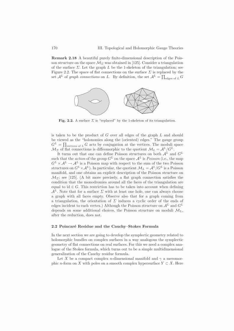
170 III. Topological and Holomorphic Gauge Theories
Remark 2.18 A beautiful purely finite-dimensional description of the Pois-son structure on the space MΣ was obtained in [125]. Consider a triangulationof the surface Σ. Let the graph L be the 1-skeleton of the triangulation; seeFigure 2.2. The space of flat connections on the surface Σ is replaced by theset AL of graph connections on L. By definition, the set AL =
∏
edges of L G
Fig. 2.2. A surface Σ is “replaced” by the 1-skeleton of its triangulation.
is taken to be the product of G over all edges of the graph L and shouldbe viewed as the “holonomies along the (oriented) edges.” The gauge groupGL =
∏
vertices of L G acts by conjugation at the vertices. The moduli spaceMΣ of flat connections is diffeomorphic to the quotient ML = AL/GL.
It turns out that one can define Poisson structures on both AL and GL
such that the action of the group GL on the space AL is Poisson (i.e., the mapGL ×AL → AL is a Poisson map with respect to the sum of the two Poissonstructures on GL×AL). In particular, the quotient ML = AL/GL is a Poissonmanifold, and one obtains an explicit description of the Poisson structure onMΣ ; see [125]. (A bit more precisely, a flat graph connection satisfies thecondition that the monodromies around all the faces of the triangulation areequal to id ∈ G. This restriction has to be taken into account when definingAL. Note that for a surface Σ with at least one hole, one can always choosea graph with all faces empty. Observe also that for a graph coming froma triangulation, the orientation of Σ induces a cyclic order of the ends ofedges incident to each vertex.) Although the Poisson structure on AL and GL
depends on some additional choices, the Poisson structure on moduli ML,after the reduction, does not.
2.2 Poincare Residue and the Cauchy–Stokes Formula
In the next section we are going to develop the symplectic geometry related toholomorphic bundles on complex surfaces in a way analogous the symplecticgeometry of flat connections on real surfaces. For this we need a complex ana-logue of the Stokes formula, which turns out to be a simple multidimensionalgeneralization of the Cauchy residue formula.
Let X be a compact complex n-dimensional manifold and γ a meromor-phic n-form on X with poles on a smooth complex hypersurface Y ⊂ X. Here
2. Poisson Structures on Moduli Spaces 171
and below we consider forms with logarithmic singularities only, i.e., formswith first-order poles. Let z : U → C be a function defining Y in a neighbor-hood U ⊂ X of some point p ∈ Y . Then locally in U the n-form γ can bedecomposed into the sum
γ =dz
z∧ α+ β ,
where α and β are, respectively, holomorphic (n− 1)-form and n-form in U .
Exercise 2.19 Show that the restriction α|Y is a well-defined holomorphic(n − 1)-form on Y , that is, α|Y is independent of the choice of z. (Hint: uselocal coordinates.)
Definition 2.20 The holomorphic (n − 1)-form α|Y on Y is called thePoincare residue of the meromorphic form γ and is denoted by resY γ.
Note that for the case of top-degree meromorphic forms having singular-ities on smooth divisors, which we consider here, a logarithmic singularity isthe same as a first-order pole. In the situation of a nonsmooth divisor of polesone should keep the formulation “γ with logarithmic singularities.”
Theorem 2.21 (Cauchy–Stokes formula, [151, 133]) Let X,Y , and γbe as above, and let u be a smooth (n− 1)-form on X. Then the form γ ∧ duis L1-integrable on X and
∫
X
γ ∧ du = 2πi∫
Y
resY γ ∧ u .
Proof. This formula is proved by applying the Stokes formula to reduce theintegral to the tubular neighborhood of Y , and then by using the standardCauchy formula in the transversal direction to Y , whence the name.
Let z be a coordinate function locally defining Y . To see that γ ∧ duis integrable, observe that γ ∧ du grows like 1/|z| as z → 0. Since the realcodimension of Y in X equals 2, the 2n-form γ ∧ du is indeed integrable onX.
To calculate the integral, choose some tubular neighborhood Uε of radiusε for the manifold Y (see Figure 2.3). Then by definition of the improperintegral we have∫
X
γ ∧ du := limε→0
∫
X\Uε
γ ∧ du = − limε→0
∫
∂Uε
γ ∧ u = limε→0
∫
Y
∫
|z|=ε
γ ∧ u ,
where we have used the Stokes theorem to reduce the integral over X \ Uε toan integral over its boundary. Note that the boundary ∂(X \ Uε) is orientedby an outer normal, which is an inner normal for the tubular neighborhood:

172 III. Topological and Holomorphic Gauge Theories
∂(X \ Uε) = −∂Uε. This orientation implies the positive (counterclockwise)orientation of the contour |z| = ε.
Finally, by decomposing γ = dzz ∧ α + β and using the Cauchy integral
formula in the z-direction we obtain
limε→0
∫
Y
∫
|z|=ε
γ ∧ u = 2πi∫
Y
α ∧ u = 2πi∫
Y
resY γ ∧ u ,
while the term involving β ∧ u vanishes as ε → 0.
Y
Uε
X
Fig. 2.3. A tubular neighborhood Uε of the polar divisor Y ⊂ X.
Another way to rewrite the Cauchy–Stokes formula is to use ∂u instead ofdu:
∫
X
γ ∧ ∂u = 2πi∫
Y
resY γ ∧ u ,
since it is only the (0, n− 1)-part of the form u that is essential here.
Remark 2.22 Theorem 2.21 can be extended to the case in which themeromorphic n-form γ has first-order poles on a normal crossing divisorY = ∪iYi ⊂ X. (A normal crossing divisor means that the smooth irreduciblecomponents Yi of Y , each one appearing with multiplicity one, intersect gener-ically.) Analogously to Definition 2.20, one can define the residue resYi
γ oneach component of Y . The resulting (n−1)-forms resYi
γ are meromorphic onYi and have first-order poles at the intersections Yi,j = Yi ∩ Yj . One can con-sider the repeated Poincare residue of γ at Yi,j . Let zi = 0 and zj = 0 be localequations in X of the components Yi and Yj respectively. Then representingγ as γ = dzi
zi∧ dzj
zj∧ α+ β, one finds that
resi,j γ := resYi,j(resYi
γ) = reszj=0
(
reszi=0dzi
zi∧ dzj
zj∧ α
)
= α|Yi,j.
Note that the sign of the repeated residue depends on the order in which thelatter was taken:
resi,j γ = − resj,i γ .
We shall denote by res γ the collection of (n − 1)-forms resYiγ, the residues
of γ at the components Yi of the normal crossing divisor Y = div∞ γ.
2. Poisson Structures on Moduli Spaces 173
Remark 2.23 We also note that for the Cauchy–Stokes formula above, thepolar divisor plays the role of the boundary in the usual Stokes formula. In thesame spirit, the meromorphic n-form can be seen as a “complex analogue” ofan orientation of a real manifold. We will encounter similar analogies betweennotions from differential topology and complex analysis in subsequent sections.
2.3 Moduli Spaces of Holomorphic Bundles
Let S be a compact complex surface (dimC S = 2) and let G be a simply con-nected complex reductive group (G ⊂ GL(n,C)). In this section, we describe aPoisson structure on the moduli space of (stable) holomorphic vector bundleson S with the structure group G.13 This will be done by analogy with ourconsiderations of the moduli space of flat connections on a Riemann surface inSection 2.1. The basic idea for this analogy is to replace the “real” notions oforientation and boundary of a Riemann surface by their “complex analogues”:a meromorphic 2-form on the surface (thought of as a “complex orientation”of S) and its divisor of poles (playing the role of the “boundary” of S); seeRemark 2.23.
On the complex surface S we fix some meromorphic 2-form β that has onlypoles of the first order and whose polar divisor P ⊂ S is a smooth curve inS. Let us assume additionally that β has no zeros. (The latter corresponds tothe smoothness of a real surface: we will see below that zeros of the 2-form βon a complex manifold would correspond to singularities of a real manifold).If it happens that β has neither zeros nor poles (i.e., S is “smooth, oriented,without boundary”) this means that we are dealing with either a K3 or anabelian surface S. If the 2-form β is meromorphic, then S is a complex Poissonsurface, since the bivector field dual to β defines a holomorphic Poisson struc-ture on S.
For the meromorphic 2-form β without zeros, its polar divisor P is ananticanonical divisor on S, and it has to be an elliptic curve or the union ofseveral nonintersecting elliptic curves. (Indeed, in this case, resP β defines anonvanishing holomorphic 1-form on P .) These elliptic curves can be seen asthe analogues of the circles constituting the boundary components of a smoothreal surface. An example of such is S = CP
2 with a smooth cubic P as ananticanonical divisor. (As a matter of fact, many Fano surfaces admit such aform β, i.e., fall into this class. The considerations below can also be extendedwith minimal changes to the case of a nonsmooth divisor P , in particular,to P consisting of several components intersecting transversally. Example: forS = CP
2 with β = dx ∧ dy/xy, the divisor P is a union of three CP1’s.)
Exercise 2.24 Prove that if a meromorphic form β is nonvanishing, so is itsresidue resP β. (Hint: use local coordinates.)13 As before, when speaking of a moduli space we shall always mean its nonsingular
part. Here under the moduli space we understand a local universal family near asmooth point.
174 III. Topological and Holomorphic Gauge Theories
Now let E be a smooth G-bundle over the surface S that can be en-dowed with a holomorphic structure, and let EndE be the correspond-ing bundle of endomorphisms with fiber g = Lie(G). Furthermore, let AS
denote the infinite-dimensional affine space of smooth (0, 1)-connections (or∂-connections) in E. Finally, let us choose a reference holomorphic structure,i.e., a (0, 1)-connection ∂ 0 such that ∂ 2
0 = 0. Then the space AS can be iden-tified with the vector space Ω0,1(S,EndE) of (EndE)-valued (0, 1)-forms onS, i.e.,
AS = ∂ 0 +A |A ∈ Ω0,1(S,EndE) .In what follows, instead of ∂ 0, we shall write simply ∂, keeping in mind thatthis corresponds to a reference holomorphic structure in E when it applies tosections of E or associated bundles.
Definition 2.25 The affine space AS possesses a natural holomorphic sym-plectic structure given by
ωC(δ1A, δ2A) =∫
S
β ∧ tr(δ1A ∧ δ2A) ,
where β is the meromorphic 2-form of S (i.e., the “complex orientation” onS), δ1A and δ2A are two tangent vectors to the affine space AS at the point∂+A, and tr(· ∧ ·) stands for the wedge product on S and the nondegeneratepairing on g.
Recall that a holomorphic symplectic structure on a complex manifold isdefined by a holomorphic closed 2-form on it that is nondegenerate over C.(Note, for instance, that the 2-form dz ∧ dw defines a holomorphic symplecticstructure in C
2, but it is not symplectic in R4 C
2 as a 2-form over R, since itis of rank 2.) In the infinite-dimensional context, the nondegeneracy is alwaysunderstood as the absence of a tangent vector skew-orthogonal to all others;see Definition I.4.4.
Following this definition, we can appropriately “complexify” the construc-tions for moduli of flat connections from Section 2.1 step by step. Abusingnotation, let us denote by GS the group of gauge transformations in E, i.e,the group of automorphisms of the smooth bundle E.
Exercise 2.26 Prove that the symplectic structure ωC is invariant with re-spect to the gauge transformations
A → gAg−1 − ∂gg−1 ,
for any g ∈ GS .
The infinitesimal gauge transformations form the Lie algebra gS =Γ (S,EndE), where Γ denotes the space of C∞-sections. As before, they aregenerated by certain Hamiltonian functions on the symplectic manifold AS .

2. Poisson Structures on Moduli Spaces 175
Proposition 2.27 An infinitesimal gauge transformation ε is generated bythe Hamiltonian function
Hε(A) =∫
S
β ∧ tr(ε(∂A+A ∧A)) − 2πi∫
P
resP β ∧ tr(εA) .
Proof. The only modification in comparison with the proof of Proposition2.3 is that now we are going to use the Cauchy–Stokes formula instead of theusual Stokes formula. Indeed, now we have
δHε(A) =∫
S
β ∧ tr (ε δF (A)) − 2πi∫
P
resP β ∧ tr(ε δA)
=∫
S
β ∧ tr(ε∇A δA) − 2πi∫
P
resP β ∧ tr (ε δA)
=∫
S
β ∧ tr(
δA ∧∇A ε)
.
Here F (A) := ∂A+A∧A is the curvature, ∇A ε := ∂ε−[ε, A] is the infinitesimalgauge transformation of a (0, 1)-connection ∂ +A by the element ε ∈ gS , and∇A δA = ∂ δA− [δA,A].
Similarly, the commutation relations for these Hamiltonians with respectto the holomorphic Poisson structure induced by ω become centrally extended:
Hε1 ,Hε2 = H[ε1,ε2] + c(ε1, ε2) ,
where c is the following 2-cocycle on the Lie algebra gS :
Proposition 2.28 The value of the cocycle c on a pair of infinitesimal gaugetransformations ε1, ε2 ∈ gS is given by
c(ε1, ε2) = 2πi∫
P
resP β ∧ tr(ε1 ∂ε2) .
Remark 2.29 Recall that a smooth divisor P must be an elliptic curve (ora union of such), while the residue resP β is a holomorphic 1-form on P . InSection II.5 we have used the same cocycle to construct a central extensiongP of the double loop group gP . This suggests that the centrally extended(elliptic) Lie algebra gP should play a similar role in the theory of holomorphicbundles on complex surfaces to that played by the centrally extended loopalgebras (the affine Lie algebras) in the theory of flat connections on Riemannsurfaces.
Let gS,β denote the Lie algebra of gauge transformations of the bundle Eover the surface S, which is centrally extended by the cocycle c from Proposi-tion 2.28, and let GS,β be the corresponding group. (One can consider any of
176 III. Topological and Holomorphic Gauge Theories
the possible central extensions of the group GS : it is only the Lie algebra thatmatters here.) The infinite-dimensional space gS,β is the space of pairs (ε, a),where ε is a g-valued function on the surface S and a is a complex number.
Definition 2.30 The (smooth) dual (gS,β)∗ to the algebra gS,β is the spaceof triples (F,C, λ), where F is an (EndE)-valued (0, 2)-form on S, C is an(EndE)-valued (0, 1)-form on the “boundary” P of the surface S (i.e., on thepolar divisor of the 2-form β), and λ is a complex number. The nondegeneratepairing 〈 , 〉 between the spaces gS,β and (gS,β)∗ is the following:
〈(F,C, λ), (ε, a)〉 =∫
S
β ∧ tr(εF ) − 2πi∫
P
resP β ∧ tr(εC) + aλ .
Let us consider the action of GS,β on the affine space AS generated by theaction of GS . This is the action by gauge transformations, while the center ofGS,β acts trivially. The following result immediately follows from Proposition2.27, similarly to the “real” case.
Proposition 2.31 ([194]) The centrally extended group GS,β of gauge trans-formations acts on the affine space AS in a Hamiltonian way. The momentmap for the action of the corresponding gauge algebra gS,β is the mappingAS → (gS,β)∗ given by the (0, 2)-curvature and by the restriction of the ∂-connection to the “boundary”:
A → (∂A+A ∧A, A|P , 1) .
As before, let us consider the group GSP of gauge transformations on S
based at the polar divisor P ,
GSP = g ∈ GS | g|P = id ,
and denote by gSP the corresponding Lie algebra. The latter can be viewed as
a subalgebra of the centrally extended Lie algebra gS,β , since the cocycle cis trivial on gS
P . Accordingly, the group GSP can be viewed as a subgroup of
the centrally extended gauge group GS,β , and we can restrict the action ofthe large group to this subgroup. A slight modification of the last propositiongives the following corollary.
Corollary 2.32 The group GSP of based gauge transformations acts on the
affine space AS in a Hamiltonian way. The moment map ΦP : AS → (gSP )∗
for this action is given by the (0, 2)-curvature:
ΦP : A → ∂A+A ∧A .
First consider the (holomorphic) Hamiltonian reduction
MS,P = AS//GSP := Φ−1
P (0)/GSP

2. Poisson Structures on Moduli Spaces 177
of the space of ∂-connections AS with respect to the group GSP . The result
will be the space of integrable ∂-connections in the bundle E on S modulogauge transformations from GS
P . Indeed, the set Φ−1P (0) consists of (0, 1)-
connections whose (0, 2)-curvature vanishes. Such connections are in one-to-one correspondence with holomorphic structures in the complex bundle E.
Thus the holomorphic Hamiltonian reduction leads us to the considera-tion of the space of all holomorphic structures in the bundle E modulo gaugeequivalences that act as the identity over P . The corresponding quotient spaceMS,P , which we consider only locally, near some of its smooth points, is, byconstruction, an (infinite-dimensional) symplectic manifold, since it comesfrom the Hamiltonian reduction of a symplectic manifold.
Remark 2.33 Before we treat the general case with a nonempty P , let uslook at the particular situation in which the meromorphic form β has no poles,i.e., it is actually a holomorphic 2-form without zeros. (As we mentioned, thiscan happen if the surface S is K3 or abelian.) If P = ∅, the group GS
P = GS
is the group of all gauge transformations on S, while (a nonsingular part of)the quotient MS,P recovers the (finite-dimensional) moduli space of (stable)holomorphic G-bundles over S. This way we obtain a “visualization” of thefollowing theorem of Mukai:
Theorem 2.34 ([283]) Let S be a K3 or abelian surface. Then the modulispace of stable holomorphic G-bundles over S admits a holomorphic symplecticstructure.
Returning to the case of a nonempty divisor P ⊂ S, consider now the spaceof holomorphic structures in a smooth bundle over a complex one-dimensionalmanifold by taking P as such a manifold and E|P as the bundle over P :
C := ∂ + C |C ∈ Ω0,1(P,EndE|P ) .
Here ∂ is understood as the restriction to P of our reference holomorphic struc-ture. The space C of holomorphic structures in a bundle on an elliptic curve(or a sum of such spaces if P consists of several disjoint components) is in factan affine subspace in a vector space dual to the elliptic Lie algebra gP,α. Thelatter Lie algebra is defined as the central extension of gP = Γ (P,EndE|P )by the cocycle
cα(ε1, ε2) = 2πi∫
P
α ∧ tr(ε1∂ε2) ;
cf. Remark 2.29. We set α := resP β, in which case we obtain the elliptic Liealgebra gP,α = gS,β/gS
P as the corresponding quotient. Consider the linear Lie–Poisson structure on the dual (gP,α)∗ of the elliptic algebra and, consequently,on its affine subspace C. Recall that the symplectic leaves of this structure (orcoadjoint orbits of the elliptic Lie group) correspond to isomorphism classes ofholomorphic bundles on P ; see Section II.5.2. We have obtained the restrictionmap
178 III. Topological and Holomorphic Gauge Theories
AS → (gP,α)∗
(respectively, the map to the product of the corresponding dual spaces if Pconsists of several connected components), which is Poisson and which factorsthrough the symplectic quotient to produce the map MS,P → (gP,α)∗.
Proposition 2.35 The mapping from the space MS,P to the coadjoint rep-resentation space (gP,α)∗, sending an integrable ∂-connection on the surfaceS to its restriction to the divisor P , is a Poisson mapping.
Proof. This mapping is essentially the moment map for the action of gaugetransformations on the polar divisor P .
In the second step, we consider the quotient of the space MS,P by thewhole group GS,β of centrally extended gauge transformations. The lattergroup acts on MS,P , since gauge transformations that are equal to the identityon P form a normal subgroup GS
P in GS,β .The quotient space
MS := MS,P / GS,β = ∂ +A ∈ AS | ∂A+A ∧A = 0/ GS,β
represents the set of isomorphism classes of holomorphic bundles on S (corre-sponding to a given underlying topological bundle E). Then, by construction,the local smooth moduli space MS of holomorphic bundles on S is a finite-dimensional Poisson manifold. Its symplectic leaves are described in terms ofcoadjoint orbits in
(
gP,α)∗ as follows.
Proposition 2.36 (i) [55, 371] The local moduli space MS of holomor-phic G-bundles on the Poisson surface S possesses a (holomorphic) Poissonstructure.
(ii) [194] The symplectic leaves of this structure are parametrized by themoduli of their restrictions to the polar divisor P ⊂ S of the nonvanishingmeromorphic 2-form β on S. (That is, a symplectic leaf is singled out byfixing the isomorphism class of the restriction to the elliptic curve P , or theisomorphism classes of restrictions to each curve if P consists of several suchcurves.)
Remark 2.37 The above proposition should not be understood in the sensethat the isomorphism classes of bundles on P can be taken arbitrarily. Ratherthey have to satisfy certain conditions that come from the fact that they ariseas restrictions of bundles defined over S.
The discussion above applies with minor modifications to the case in whichthe polar divisor P consists of several components intersecting transversally.In the latter case, the corresponding group GP,α is the extended current groupover the (reducible) complex curve P .

2. Poisson Structures on Moduli Spaces 179
2.4 Bibliographical Notes
The classical reference for the moduli space of flat connections on a Riemannsurface is the paper by Atiyah and Bott [28]. The case of a surface withboundary was studied in [83, 125]. In our exposition we follow the papers[125] and [194] for the real and complex sides of the story.
The finite-dimensional description [125] of the moduli space MΣ with thehelp of connections on graphs had various extensions and generalizations (see,e.g., [10, 184]), and it is related to recent progress in such diverse areas as [6,71, 105, 121, 122]. For a beautiful introduction and survey of the surroundingarea we refer the reader to [29].
For other finite-dimensional constructions of the symplectic moduli spacesee, e.g., [173, 183]. In [6] this space was studied by introducing the notion of agroup-valued moment map, which proved to be a powerful tool in symplecticgeometry. In Appendix A.10 we discuss torus actions and integrable systemson such moduli spaces, after [175, 120].
The Cauchy–Stokes formula can be found, in particular, in [151]. Theapproach using this formula can also be viewed as parallel to the geometriccomplexification suggested by Arnold in [14].
The symplectic structure on the moduli space of stable sheaves on a K3surface or an abelian surface was found by Mukai [283] by algebro-geometricmethods, while the holomorphic Poisson structures were discussed in [55, 371].The description of the corresponding holomorphic symplectic leaves wasobtained in [194].

180 III. Topological and Holomorphic Gauge Theories
3 Around the Chern–Simons Functional
In this section we move from surfaces to threefolds, along with connections andbundles on them. By studying the topological Chern–Simons action functionalon the space of connections on a three-dimensional manifold with boundary,we recover the definition of the symplectic structure on the moduli space of flatconnections on a compact Riemann surface. Similarly, the holomorphic Chern–Simons functional on ∂-connections over three-dimensional Fano manifolds isrelated to the holomorphic symplectic structure on the moduli spaces of stablebundles over K3 or abelian surfaces.
Furthermore, the corresponding path integrals for these Chern–Simonsfunctionals in the abelian case can be used to define the Gauss linking numberof oriented curves in three-dimensional space and its holomorphic analogue,the polar linking number of holomorphic curves.
3.1 A Reminder on the Lagrangian Formalism
A motion of a particle on a manifold can be described by the least actionprinciple. Consider an action functional
S[q] =∫ t1
t0
L(q(t), q(t), t) dt
defined on the space C[t0, t1] of smooth maps q : [t0, t1] → M of the interval[t0, t1] to the manifold M . Here L is a (time-dependent) Lagrangian function,L : TM × R → R, which we assume to depend only on t, q, and its firstderivative q := dq/dt.
For a path variation δq one can find the corresponding variation of theaction functional, i.e., the linear-in-δq term of the difference S[q + δq] − S[q]:
δS[q] =∫ t1
t0
E δq dt+ p δq|t1t0 ,
where
E :=∂L(q, q, t)
∂q− d
dt
∂L(q, q, t)∂q
and
p :=∂L(q, q, t)
∂q.
(Here and below we assume the summation over the coordinates q =(q1, . . . , qd): pδq :=
∑
j pjδqj , pj := ∂L(q, q, t)/∂qj , etc.)
Exercise 3.1 Prove the variation formula. (Hint: use integration by parts.)
This way the variation δS can be regarded as a 1-form on the infinite-dimensional space C[t0, t1] of “virtual trajectories” of the particle.
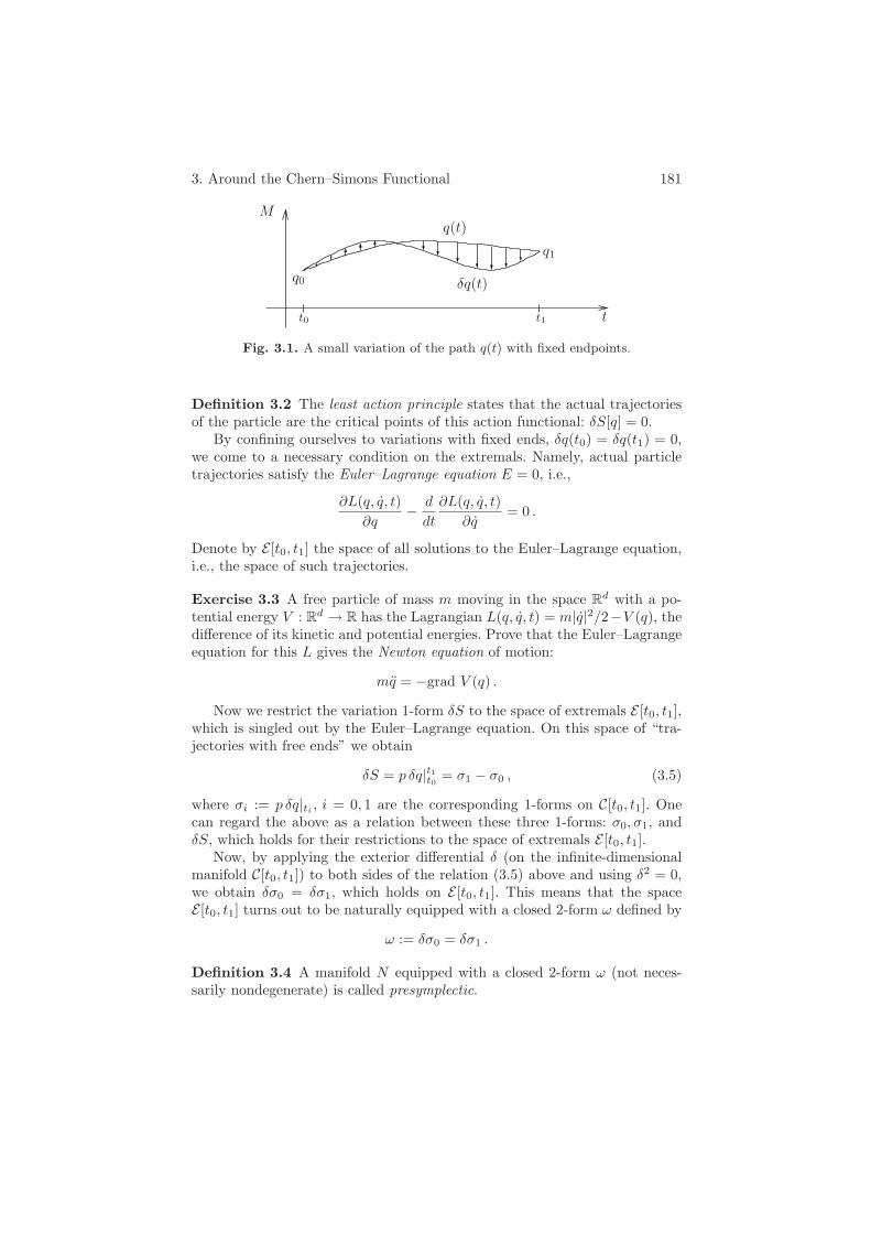
3. Around the Chern–Simons Functional 181
q(t)
δq(t)q0
M
t0 t1 t
q1
Fig. 3.1. A small variation of the path q(t) with fixed endpoints.
Definition 3.2 The least action principle states that the actual trajectoriesof the particle are the critical points of this action functional: δS[q] = 0.
By confining ourselves to variations with fixed ends, δq(t0) = δq(t1) = 0,we come to a necessary condition on the extremals. Namely, actual particletrajectories satisfy the Euler–Lagrange equation E = 0, i.e.,
∂L(q, q, t)∂q
− d
dt
∂L(q, q, t)∂q
= 0 .
Denote by E [t0, t1] the space of all solutions to the Euler–Lagrange equation,i.e., the space of such trajectories.
Exercise 3.3 A free particle of mass m moving in the space Rd with a po-
tential energy V : Rd → R has the Lagrangian L(q, q, t) = m|q|2/2−V (q), the
difference of its kinetic and potential energies. Prove that the Euler–Lagrangeequation for this L gives the Newton equation of motion:
mq = −grad V (q) .
Now we restrict the variation 1-form δS to the space of extremals E [t0, t1],which is singled out by the Euler–Lagrange equation. On this space of “tra-jectories with free ends” we obtain
δS = p δq|t1t0 = σ1 − σ0 , (3.5)
where σi := p δq|ti, i = 0, 1 are the corresponding 1-forms on C[t0, t1]. One
can regard the above as a relation between these three 1-forms: σ0, σ1, andδS, which holds for their restrictions to the space of extremals E [t0, t1].
Now, by applying the exterior differential δ (on the infinite-dimensionalmanifold C[t0, t1]) to both sides of the relation (3.5) above and using δ2 = 0,we obtain δσ0 = δσ1, which holds on E [t0, t1]. This means that the spaceE [t0, t1] turns out to be naturally equipped with a closed 2-form ω defined by
ω := δσ0 = δσ1 .
Definition 3.4 A manifold N equipped with a closed 2-form ω (not neces-sarily nondegenerate) is called presymplectic.

182 III. Topological and Holomorphic Gauge Theories
Consider the distribution of null-spaces of this 2-form in N .
Exercise 3.5 (i) Assuming that this distribution has constant rank, provethat it is integrable, i.e., it is tangent to a foliation in N .
(ii) Assuming that this null-foliation is a fibration π : N → N ′, prove thatthe base of this fibration carries a natural symplectic structure, i.e., (N ′, ω′)is a symplectic manifold such that π∗ω′ = ω.
The above discussion shows that whenever the space of extremals E [t0, t1]is a manifold, it is in fact a presymplectic manifold. However, the 2-form ω isoften degenerate. The phase space P of the particle can be described as thecorresponding symplectic manifold. (Here we implicitly assume that variousregularity conditions are satisfied to guarantee that both E [t0, t1] and thephase space are smooth manifolds.)
Exercise 3.6 Check that for the above example of a particle motion in Rd
this definition of the phase space P coincides with T ∗R
d equipped with thenatural symplectic structure.
Remark 3.7 [393, 79, 341] The discussed Lagrangian formalism can be gen-eralized to infinite-dimensional target manifolds M or to higher-dimensionaldomains instead of the interval [t0, t1]. These are the objects that a field theorydeals with. Consider, for example, a local action functional
S[ϕ] =∫
N
L(ϕ(x), ∂ϕ(x)) dnx
describing a field theory on an n-dimensional manifold N with boundary ∂N .Here x = (x1, . . . , xn) are local coordinates on N , ϕ is a map from N toa target manifold M or a section of some bundle on N , ∂ϕ are the firstderivatives of ϕ, while the Lagrangian L can depend on additional structureson N . As in the one-dimensional situation described above, one can pose avariational problem δS[ϕ] = 0, which leads to the Euler–Lagrange equations.
Suppose first that N = I × Σ, where I is an interval and a manifold Σhas dimension n− 1. One can consider t ∈ I as the time variable and identifythe field theory with an infinite-dimensional classical mechanics, where thespace of maps ϕ : Σ → M plays the role of the target. In particular, one hasa presymplectic manifold of extremals EN and the symplectic phase space Passociated to N (or, rather, to Σ).
Alternatively, one can associate the phase spaces P0 and P1 to the cor-responding boundary components ∂N = Σ1 − Σ0 of N , and equip the totalphase space P0 × P1 with the product symplectic structure. There is a nat-ural projection αN of the space EN of extremals into the product P0 × P1,since it “tautologically” projects to each factor: one describes the extremalsvia different boundary components, taking the orientation of the latter intoaccount. Then the relation 0 = δ2S = δσ1 − δσ0 that held on EN now reads
3. Around the Chern–Simons Functional 183
that the image αN (EN ) of EN is an isotropic submanifold in the symplecticmanifold P0 × P1.
Definition 3.8 A submanifold of a symplectic manifold is isotropic if therestriction of the symplectic form to this submanifold is zero.
Exercise 3.9 Let f : (N1, ω1) → (N2, ω2) be a diffeomorphism between twosymplectic manifolds. Prove that f is a symplectic map, i.e., ω1 = f∗ω2, if andonly if the graph of f is an isotropic submanifold in the symplectic manifold(N1 ×N2, ω1 ω2).
(An isotropic submanifold of maximal possible dimension, which is equalto half the dimension of the symplectic manifold, is called a Lagrangian sub-manifold; cf. Section I.4.5. This is the case for the graph of f .)
One can see that the image αN (EN ) is indeed isotropic in P0×P1, since the2-form δσ1− δσ0 is exactly the restriction of the product symplectic structureof P0 × P1 (with different orientations of the boundary components) to thisimage.
The latter formulation of the presymplectic/isotropic properties of thespace of extremals EN extends naturally to the general case of a manifoldN with boundary consisting of several components Σ1, . . . , Σk. Associate thephase space Pj to each component Σj , thinking of a neighborhood of Σj
in N as a product I × Σ. One has the relations δS = σ1 + · · · + σk andδσ1 + · · · + δσk = 0 on the space of extremals EN , where σj stands for thecontribution of the corresponding boundary component. The latter shows thatthe image αN (EN ) under the natural map αN : EN → P1 × · · · × Pk isisotropic with respect to the product symplectic structure on the phase spaceP1 × · · · × Pk. We refer to [341, 79] for more details.
Remark 3.10 The philosophy of holomorphic orientation (see Sections 2.2and 2.3) can be applied to field-theoretic notions in the following way. Supposewe have an action functional
S[ϕ] =∫
M
L(ϕ, ∂ϕ) dnx
on smooth fields ϕ (e.g., functions, connections, etc.) on a real (oriented)manifold M , and this functional is defined by an n-form Ldnx, which dependson the fields and their derivatives.
Then one can suggest the following complex analogue SC of the actionfunctional S for a complex n-dimensional manifold X equipped with a “polarorientation,” i.e., with a holomorphic or meromorphic n-form µ:
SC[ϕ] :=∫
X
µ ∧ L(ϕ, ∂ϕ) dnx .
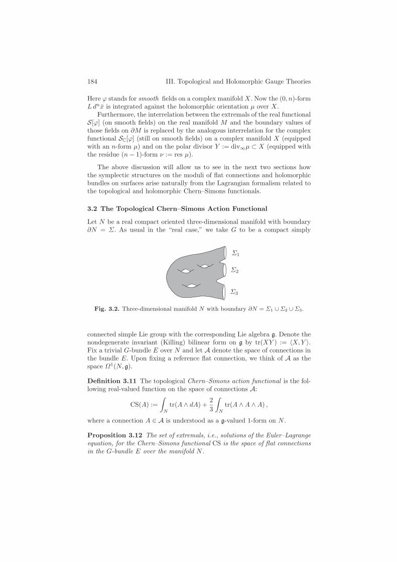
184 III. Topological and Holomorphic Gauge Theories
Here ϕ stands for smooth fields on a complex manifold X. Now the (0, n)-formLdnx is integrated against the holomorphic orientation µ over X.
Furthermore, the interrelation between the extremals of the real functionalS[ϕ] (on smooth fields) on the real manifold M and the boundary values ofthose fields on ∂M is replaced by the analogous interrelation for the complexfunctional SC[ϕ] (still on smooth fields) on a complex manifold X (equippedwith an n-form µ) and on the polar divisor Y := div∞µ ⊂ X (equipped withthe residue (n− 1)-form ν := res µ).
The above discussion will allow us to see in the next two sections howthe symplectic structures on the moduli of flat connections and holomorphicbundles on surfaces arise naturally from the Lagrangian formalism related tothe topological and holomorphic Chern–Simons functionals.
3.2 The Topological Chern–Simons Action Functional
Let N be a real compact oriented three-dimensional manifold with boundary∂N = Σ. As usual in the “real case,” we take G to be a compact simply
Σ3
Σ1
Σ2
Fig. 3.2. Three-dimensional manifold N with boundary ∂N = Σ1 ∪ Σ2 ∪ Σ3.
connected simple Lie group with the corresponding Lie algebra g. Denote thenondegenerate invariant (Killing) bilinear form on g by tr(XY ) := 〈X,Y 〉.Fix a trivial G-bundle E over N and let A denote the space of connections inthe bundle E. Upon fixing a reference flat connection, we think of A as thespace Ω1(N, g).
Definition 3.11 The topological Chern–Simons action functional is the fol-lowing real-valued function on the space of connections A:
CS(A) :=∫
N
tr(A ∧ dA) +23
∫
N
tr(A ∧A ∧A) ,
where a connection A ∈ A is understood as a g-valued 1-form on N .
Proposition 3.12 The set of extremals, i.e., solutions of the Euler–Lagrangeequation, for the Chern–Simons functional CS is the space of flat connectionsin the G-bundle E over the manifold N .

3. Around the Chern–Simons Functional 185
Proof. For a small variation δA of a connection A ∈ A the correspondingvariation of the functional is
δCS =∫
N
tr(δA ∧ dA) +∫
N
tr(A ∧ dδA) + 2∫
N
tr(δA ∧A ∧A)
=∫
N
d tr(A ∧ δA) + 2∫
N
tr (δA ∧ (dA+A ∧A))
=∫
∂N
tr(A ∧ δA) + 2∫
N
tr (δA ∧ (dA+A ∧A)) ,
where at the last step we used the Stokes formula.By imposing the boundary condition δA|∂N = 0 on variations δA, we
obtain the Euler–Lagrange equation
dA+A ∧A = 0 ,
i.e., the equation of vanishing curvature F (A) = 0 on N . Hence the space ofsolutions of this equation is exactly the space of flat connections on the realthreefold N .
The first term in the above calculation of δCS gives the boundary contri-bution, the 1-form
∑
σj on the extremals, where the summation is taken overthe boundary components of ∂N . Take N = I×Σ to be a finite cylinder overa closed two-dimensional surface Σ. Then the presymplectic structure on thespace of flat connections on N , i.e., on the extremals for our action functional,is ω = δσ for
σ :=∫
Σ
tr(a ∧ δa) ,
where a := A|Σ denotes the restriction of a flat connection A from the man-ifold N to either of its boundary components Σ. (Here we omit the indexj = 0, 1 for σj , since ω = δσ0 = δσ1.)
Exercise 3.13 Verify that the 2-form ω = δσ is degenerate on the space offlat connections on the surface Σ exactly along the gauge equivalence classesof the connections a. (Hint: the 2-form δσ =
∫
Σtr(δa∧δa) is the restriction
of the canonical 2-form ω from the set of all connections to the subset of flatconnections on Σ; cf. Definition 2.1.)
Thus the moduli space of flat connections MΣ on the surface Σ appearsas the natural symplectic (or phase) space for this presymplectic space offlat connections on Σ, and we obtain yet another definition of the symplecticstructure on MΣ from Section 2.1.
Corollary 3.14 The moduli space MΣ of flat connections on a surface Σis naturally symplectic as the phase space for extremals of the Chern–Simonsaction functional for connections on the threefold N = I ×Σ.
186 III. Topological and Holomorphic Gauge Theories
Remark 3.15 To see why this action functional is called topological wenow check the invariance property of the Chern–Simons action with re-spect to gauge transformations of the connections. Let M be a compactthree-dimensional manifold without boundary and suppose that A and ˜A areconnections in a G-bundle over M that are sent to each other by a gaugetransformation g:
˜A = gAg−1 − dgg−1 .
Then the Chern–Simons actions for them are related as follows:
CS( ˜A) = CS(A) +13
∫
M
tr(
g−1dg ∧ g−1dg ∧ g−1dg)
.
Recall that the 3-form 124π2 tr(g−1dg)∧3 is the pullback under the map g :
M → G of an integral closed 3-form η on the compact simply connectedsimple Lie group G (see Proposition 2.16 in Appendix A.2; cf. Section II.1.3).Thus the integral of this form depends only on topological properties of themap g and can be expressed as
124π2
∫
M
tr(g−1dg)∧3 =∫
M
g∗η ,
which is an integer, since the 3-form η generates H3(G,Z). The latter impliesthat the exponential exp
(
i4π CS(A)
)
is gauge invariant:
i
4πCS( ˜A) − i
4πCS(A) = 2πi · 1
24π2
∫
M
tr(g−1dg)∧3 ∈ 2πi · Z .
Remark 3.16 An interesting integer-valued invariant for a homology3-sphere M was introduced by Casson and is closely related to the gauge-theoretic constructions above [70]. Roughly speaking, the Casson invari-ant Cas(M) is defined as the algebraic number of the conjugacy classes ofirreducible SU(2)-representations of the fundamental group π1(M). In otherwords, it counts the number of irreducible flat SU(2)-connections on M mod-ulo conjugation. The homology restriction on the threefold M is related tothe fact that if H1(M) = 0, then the moduli space of flat connections on Mmight not be zero-dimensional, and in particular, it would not consist of afinite number of points. The reason for restricting to SU(2) is clarified in thefollowing exercise.
Exercise 3.17 Show that the only reducible representation ρ : π1(M) →SU(2) is the trivial one. (Hint: Reducible representations of π1(M) in SU(2)are necessarily abelian and hence factor through the homology H1(M). Thishomology group is trivial for a homology 3-sphere.)
Now consider a Heegaard splitting of M into two handlebodies M =M1 ∪Σ M2 glued together along their common boundary, an embedded sur-face Σ ⊂ M . Consider the moduli space MΣ of flat connections in the trivial
3. Around the Chern–Simons Functional 187
SU(2)-bundle on the surface Σ. Define two submanifolds L1 and L2 of thesymplectic manifold MΣ as those (equivalence classes of) flat connections onthe surface Σ that extend to M1 and M2 respectively. One can show that thesesubmanifolds are Lagrangian. Their intersection points L1 ∩L2 correspond toflat connections extendable to the whole of M . Thus the Casson invariant isdefined as the intersection number of these submanifolds,
Cas(M) = #(L1, L2) ,
where we assume that the submanifolds intersect transversally, and excludethe intersection corresponding to the trivial representation; see details, forexample, in [364].
3.3 The Holomorphic Chern–Simons Action Functional
A complex three-dimensional manifold X equipped with a nowhere vanish-ing meromorphic 3-form µ can be regarded as a complex analogue of areal oriented manifold with boundary, following the general philosophy thatwe adopted in Sections 2.2 and 2.3. Accordingly, one can complexify theLagrangian formalism to this situation. Here we define a holomorphic analogueof the Chern–Simons action functional for (X,µ) and relate it to Mukai’s holo-morphic symplectic structures on moduli of holomorphic bundles over complexsurfaces, following [195, 85].
Let GC be a complex simple and simply connected Lie group and EC acomplex GC-bundle over the manifold X. As before, let us denote by AX
Cthe
space of (0, 1)-connections in the bundle EC.
Definition 3.18 The holomorphic Chern–Simons action functional CSC :AX
C→ C is defined via
CSC(A) :=∫
X
µ ∧(
〈A ∧ ∂A〉 +23〈A ∧A ∧A〉
)
for any (0, 1)-connection A ∈ AXC
thought of as a gC-valued (0, 1)-form on X.As usual, we assume that the 3-form µ has only first-order poles, and hencethe integral above is well defined.
Proposition 3.19 The extremals of the holomorphic Chern–Simons func-tional are holomorphic structures in the complex bundle EC.
Proof. Indeed, in the same way as in the real case and by using the Cauchy–Stokes formula we come to the Euler–Lagrange equation
∂A+A ∧A = 0

188 III. Topological and Holomorphic Gauge Theories
in the holomorphic setting. Its solutions are (0, 1)-connections A with van-ishing (0, 2)-curvature, F 0,2(A) = 0, and each such connection defines thecorresponding holomorphic structure in the complex bundle EC.
Consider now the “boundary term” of the variation δCSC, which now de-scends to the polar divisor of the meromorphic 3-form µ. Denote this polardivisor by Y := div∞µ ⊂ X. Note that the residue ν := resY µ is a nonva-nishing 2-form on the divisor Y , since µ itself is nonvanishing (see Exercise2.19). In particular, the canonical bundle of Y has to be trivial, so that Y iseither a K3 surface or a complex torus.
To define the presymplectic structure in the real case we considered acylinder M = I ×Σ over a Riemann surface Σ. Here we look at the complexanalogue of such a cylinder. Namely, let X = CP
1 × Y be the product ofCP
1 and a K3 surface or abelian surface Y . Suppose that Y is endowedwith a holomorphic (necessarily nonvanishing) 2-form ν, and consider themeromorphic 3-form µ = (dz/z) ∧ ν on X, where dz/z is a 1-form on thecomplex line CP
1. One can see that ν = resz=0 µ = − resz=∞ µ.Now the variation of the holomorphic Chern–Simons functional satisfies
the relation δCSC = σ0,C + σ∞,C on the space of extremals, which are theintegrable (0, 1)-connections on X, i.e., the connections with vanishing (0, 2)-curvature. Here σ0,C and σ∞,C stand for the contributions of the correspondingcomponents z = 0 and z = ∞ of the polar divisor of µ.
This allows us to introduce the holomorphic presymplectic structure ωC =δσC on the “boundary values” of the extremals, i.e., on the space of integrableconnections on the surface Y . Explicitly, the holomorphic 1-form σC is
σC :=∫
Y
ν ∧ tr(a ∧ δa) ,
where a := A|z=0 is the restriction of a (0, 1)-connection A in EC from thethreefold X to the surface Y (understood as one component z = 0×Y ⊂ Xof the polar divisor of µ), δa is the corresponding variation of a, and ν =resz=0 µ is a holomorphic 2-form on Y .
One can show that, similarly to the real case, the presymplectic structureωC is degenerate along the orbits of the action of the complex group of gaugetransformations GY
Con integrable (0, 1)-connections (i.e., holomorphic struc-
tures) in the bundle EC over Y . After taking the quotient with respect to thegroup action, we obtain a nondegenerate holomorphic symplectic structure onthe moduli space of (stable) holomorphic bundles on the K3 or abelian sur-face Y . (Here, as usual, we are concerned with the moduli space only locallyaround a smooth point.) Thus the holomorphic Lagrangian formalism givesan alternative approach to Mukai’s result discussed before:
Theorem 3.20 ([283]) There exists a holomorphic symplectic structure ωC
on the moduli space MY of stable holomorphic GC-bundles over a K3 orabelian surface Y .
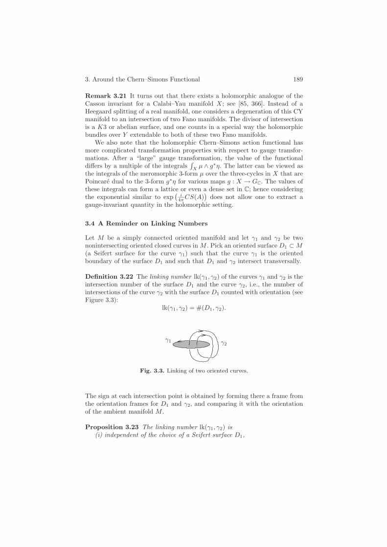
3. Around the Chern–Simons Functional 189
Remark 3.21 It turns out that there exists a holomorphic analogue of theCasson invariant for a Calabi–Yau manifold X; see [85, 366]. Instead of aHeegaard splitting of a real manifold, one considers a degeneration of this CYmanifold to an intersection of two Fano manifolds. The divisor of intersectionis a K3 or abelian surface, and one counts in a special way the holomorphicbundles over Y extendable to both of these two Fano manifolds.
We also note that the holomorphic Chern–Simons action functional hasmore complicated transformation properties with respect to gauge transfor-mations. After a “large” gauge transformation, the value of the functionaldiffers by a multiple of the integrals
∫
Xµ ∧ g∗η. The latter can be viewed as
the integrals of the meromorphic 3-form µ over the three-cycles in X that arePoincare dual to the 3-form g∗η for various maps g : X → GC. The values ofthese integrals can form a lattice or even a dense set in C; hence consideringthe exponential similar to exp
(
i4πCS(A)
)
does not allow one to extract agauge-invariant quantity in the holomorphic setting.
3.4 A Reminder on Linking Numbers
Let M be a simply connected oriented manifold and let γ1 and γ2 be twononintersecting oriented closed curves in M . Pick an oriented surface D1 ⊂ M(a Seifert surface for the curve γ1) such that the curve γ1 is the orientedboundary of the surface D1 and such that D1 and γ2 intersect transversally.
Definition 3.22 The linking number lk(γ1, γ2) of the curves γ1 and γ2 is theintersection number of the surface D1 and the curve γ2, i.e., the number ofintersections of the curve γ2 with the surface D1 counted with orientation (seeFigure 3.3):
lk(γ1, γ2) = #(D1, γ2).
γ2γ1
Fig. 3.3. Linking of two oriented curves.
The sign at each intersection point is obtained by forming there a frame fromthe orientation frames for D1 and γ2, and comparing it with the orientationof the ambient manifold M .
Proposition 3.23 The linking number lk(γ1, γ2) is(i) independent of the choice of a Seifert surface D1,
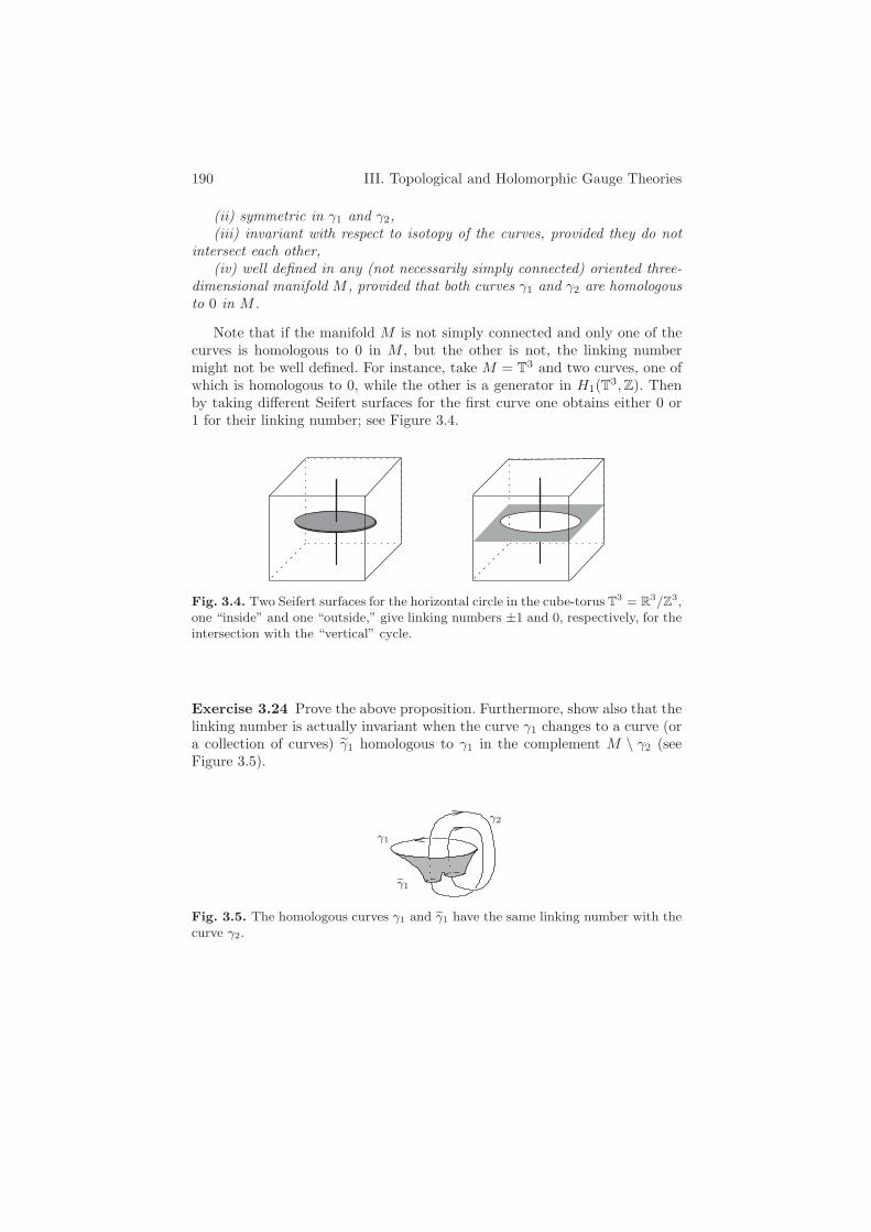
190 III. Topological and Holomorphic Gauge Theories
(ii) symmetric in γ1 and γ2,(iii) invariant with respect to isotopy of the curves, provided they do not
intersect each other,(iv) well defined in any (not necessarily simply connected) oriented three-
dimensional manifold M , provided that both curves γ1 and γ2 are homologousto 0 in M .
Note that if the manifold M is not simply connected and only one of thecurves is homologous to 0 in M , but the other is not, the linking numbermight not be well defined. For instance, take M = T
3 and two curves, one ofwhich is homologous to 0, while the other is a generator in H1(T3,Z). Thenby taking different Seifert surfaces for the first curve one obtains either 0 or1 for their linking number; see Figure 3.4.
Fig. 3.4. Two Seifert surfaces for the horizontal circle in the cube-torus T3 = R
3/Z3,
one “inside” and one “outside,” give linking numbers ±1 and 0, respectively, for theintersection with the “vertical” cycle.
Exercise 3.24 Prove the above proposition. Furthermore, show also that thelinking number is actually invariant when the curve γ1 changes to a curve (ora collection of curves) γ1 homologous to γ1 in the complement M \ γ2 (seeFigure 3.5).
γ1
γ1
γ2
Fig. 3.5. The homologous curves γ1 and γ1 have the same linking number with thecurve γ2.
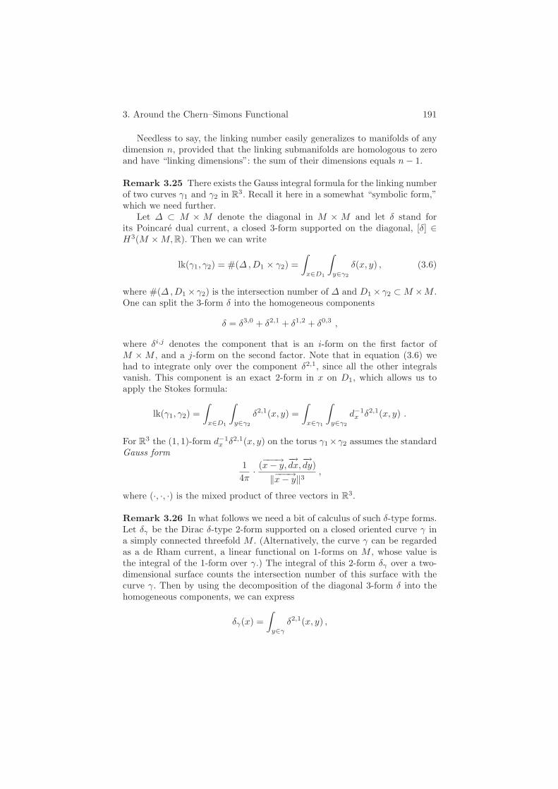
3. Around the Chern–Simons Functional 191
Needless to say, the linking number easily generalizes to manifolds of anydimension n, provided that the linking submanifolds are homologous to zeroand have “linking dimensions”: the sum of their dimensions equals n− 1.
Remark 3.25 There exists the Gauss integral formula for the linking numberof two curves γ1 and γ2 in R
3. Recall it here in a somewhat “symbolic form,”which we need further.
Let ∆ ⊂ M × M denote the diagonal in M × M and let δ stand forits Poincare dual current, a closed 3-form supported on the diagonal, [δ] ∈H3(M ×M,R). Then we can write
lk(γ1, γ2) = #(∆,D1 × γ2) =∫
x∈D1
∫
y∈γ2
δ(x, y) , (3.6)
where #(∆,D1 × γ2) is the intersection number of ∆ and D1 × γ2 ⊂ M ×M .One can split the 3-form δ into the homogeneous components
δ = δ3,0 + δ2,1 + δ1,2 + δ0,3 ,
where δi,j denotes the component that is an i-form on the first factor ofM ×M , and a j-form on the second factor. Note that in equation (3.6) wehad to integrate only over the component δ2,1, since all the other integralsvanish. This component is an exact 2-form in x on D1, which allows us toapply the Stokes formula:
lk(γ1, γ2) =∫
x∈D1
∫
y∈γ2
δ2,1(x, y) =∫
x∈γ1
∫
y∈γ2
d−1x δ2,1(x, y) .
For R3 the (1, 1)-form d−1
x δ2,1(x, y) on the torus γ1×γ2 assumes the standardGauss form
14π
· (−−−→x− y,−→dx,
−→dy)
‖−−−→x− y‖3,
where (·, ·, ·) is the mixed product of three vectors in R3.
Remark 3.26 In what follows we need a bit of calculus of such δ-type forms.Let δγ be the Dirac δ-type 2-form supported on a closed oriented curve γ ina simply connected threefold M . (Alternatively, the curve γ can be regardedas a de Rham current, a linear functional on 1-forms on M , whose value isthe integral of the 1-form over γ.) The integral of this 2-form δγ over a two-dimensional surface counts the intersection number of this surface with thecurve γ. Then by using the decomposition of the diagonal 3-form δ into thehomogeneous components, we can express
δγ(x) =∫
y∈γ
δ2,1(x, y) ,

192 III. Topological and Holomorphic Gauge Theories
where we denote the coordinates on the first and the second factors of M×Mby x and y respectively. Choose a surface D ⊂ M whose boundary is γ = ∂D.Similarly, we can define the δ-type 1-form supported on the surface D by
δD(x) =∫
y∈D
δ1,2(x, y) .
The relation ∂D = γ is equivalent to the relation between the correspondingδ-forms: dxδD(x) = δγ(x), due to the Stokes theorem, or more explicitly,
δγ(x) =∫
y∈D
dx(δ1,2)(x, y) ,
where dx denotes the exterior derivative applied to the x-coordinates only.Finally, if γ1 and γ2 are two nonintersecting curves, we have
lk(γ1, γ2) =∫
x∈D1
δγ2(x) =∫
M
δD1(x) ∧ δγ2(x) =∫
M
δD1 ∧ dδD2 , (3.7)
where ∂D2 = γ2. The latter form suggests a common nature of the linkingnumber and the A ∧ dA-part of the Chern–Simons functional, which we aregoing to study below.
3.5 The Abelian Chern–Simons Path Integral and LinkingNumbers
We start with a reminder on finite-dimensional Gaussian integrals. Let (x,Qx)be a symmetric negative-definite form in the Euclidean R
n. The classicalGauss integral
∫
R
exp(−qx2/2)dx =√
2π/q
has the multidimensional analogue
∫
Rn
e12 (x,Qx) dnx =
(
(2π)n
det(−Q)
)12
.
Now fix a vector J ∈ Rn and consider the integral
ZQ(J) :=∫
Rn
e12 (x,Qx)+(x,J) dnx =
∫
Rn
eSJ (x) dnx
corresponding to the shift SJ(x) := 12 (x,Qx) + (x, J) of the quadratic form
by a linear term. (The initial integral is ZQ(0).) This integral can easily besolved by completing the square. Indeed, let x0 be a solution of the equationQx0 + J = 0, i.e., x0 = −Q−1J . Then by introducing a shifted variablex = x−x0 and using the translation invariance of the measure dnx, we obtain
3. Around the Chern–Simons Functional 193
ZQ(J) =∫
Rn
eSJ (x+x0) dnx
=∫
Rn
exp1
2(x+ x0, Q(x+ x0)) + (x+ x0, J)
dnx
=∫
Rn
exp1
2(x, Qx) +
12(x0, Qx0) + (x0, J)
dnx
= eSJ (x0)
∫
Rn
e12 (x,Qx) dnx = e
12 (x0,J) ZQ(0) .
Thus, we have
ZQ(J)ZQ(0)
= eSJ (x0) = e12 (x0,J) = e−
12 (Q−1J,J) . (3.8)
Remark 3.27 When the space Rn is replaced by some infinite-dimensional
vector space, the integrals defining ZQ(0) and ZQ(J) usually do not makesense. However, one can “calculate” their ratio, which often turns out tobe well defined. Note that the second of the equivalent expressions forthe ratio ZQ(J)/ZQ(0) in formula (3.8) has the form exp(1
2 (x0, J)) =exp(− 1
2 (x0, Qx0)), which allows us to avoid looking for the inverse Q−1 ofthe corresponding operator in the infinite-dimensional space.
Consider an application of this idea to the abelian Chern–Simons pathintegral. Let A be the space of connections in a U(1)-bundle over a real three-dimensional simply connected manifold M without boundary. We can thinkof such connections as real-valued 1-forms on M . Denote by CS : A → R
the Chern–Simons action functional on A = Ω1(M,R), which now becomes aquadratic form
CS(A) =∫
M
A ∧ dA ,
since the group U(1) is abelian and the cubic term A ∧A ∧A vanishes. Notethat the kernel of this quadratic form is the space of exact 1-forms dΩ0 ⊂Ω1(M,R).
Fix some linear functional J on Ω1(M,R), i.e., a de Rham current on thisspace, and define
SJ(A) :=12
∫
M
A ∧ dA+∫
M
A ∧ J .
for A ∈ Ω1(M,R). We also impose the condition dJ = 0, so that the linearterm
∫
MA ∧ J is well defined on the quotient Ω1(M)/dΩ0(M). Now make
the following “formal” definition.
Definition 3.28 The abelian Chern–Simons path integral is the expression
194 III. Topological and Holomorphic Gauge Theories
ZCS(J) :=∫
Ω1/dΩ0eSJ (A) DA ,
where DA stands for a translation-invariant measure on the infinite-dimensional space Ω1(M)/dΩ0(M).
Rather than trying to define the measure and the path integral precisely,we are going to see what the above formal manipulations with Gaussian inte-grals give us in this situation, where, in a sense, the operator Q is replaced bythe outer derivative d. By formula (3.8) for the ratio ZQ(J)/ZQ(0) we obtain
ZCS(J)ZCS(0)
= eSJ (A0) = e12
∫
MA0∧J ,
where A0 is a solution of the equation dA0 + J = 0. (Recall that J is a closedcurrent on a simply connected M , and hence it is exact, i.e., this equationformally has a solution.)
Now we would like to specify the functional J on 1-forms A ∈ Ω1(M,R) tobe the integral of the form over a collection of curves in the simply connectedmanifold M . Let γi, i = 1, . . . , k, be closed oriented nonintersecting curvesin the manifold M . We set J =
∑
i qi δγi, where δγi
is the δ-type 2-form onM supported on the curve γi, while qi are real parameters. By applying thecalculus of δ-forms (see Remark 3.26) we obtain that the ratio ZCS(J)/ZCS(0)assumes the following explicit form:
ZCS(J)ZCS(0)
= exp1
2
∫
M
A0 ∧ J
= exp1
2
∫
M
A0 ∧∑
i
qi
∫
y∈γi
δ2,1(x, y)
= exp1
2
∫
M
A0 ∧∑
i
qi
∫
y∈Di
dxδ1,2(x, y)
= exp1
2
∫
M
−dA0 ∧∑
i
qi
∫
y∈Di
δ1,2(x, y)
= exp1
2
∫
M
⎛
⎝
∑
j
qj
∫
z∈γj
δ2,1(x, z)
⎞
⎠ ∧(
∑
i
qi
∫
y∈Di
δ1,2(x, y)
)
= exp1
2
∑
i,j
qiqj
∫
M
δγj(x) ∧ δDi
(x)
= exp1
2
∑
i,j
qiqj lk(γj , γi)
Here we have used the Stokes theorem, as well as the definition of A0 as asolution of the equation dA0 + J = 0.
Corollary 3.29 ([340, 318]) For the functional J defined as the integral of1-forms over a collection of curves in a threefold, the ratio ZCS(J)/ZCS(0)counts the pairwise linking numbers of these curves.
3. Around the Chern–Simons Functional 195
Note also that above, in the latter sum, we had to assume that i = j, sothat the linking number was defined. The case of self-linking is much moresubtle. It leads to divergences of the path integral and requires some additionalspecifications, such as framing, for its normalization; see [54]. The value ZCS(0)in the case without any curve corresponds to the Ray–Singer torsion of themanifold M [340].
The topological Chern–Simons path integral has a holomorphic analogue.
Definition 3.30 (cf. [390]) For a three-dimensional Calabi–Yau manifoldX with a holomorphic 3-form µ the holomorphic abelian Chern–Simons pathintegral is the expression
ZCS(J) :=∫
Ω0,1/∂Ω0,0eSCJ (A) DA ,
whereSCJ(A) :=
12
∫
X
µ ∧A ∧ ∂A+ 〈CJ,A〉
is the quadratic form shifted by the linear functional CJ on the space of(0, 1)-connections A ∈ Ω0,1(X,C).
Remark 3.31 For a complex curve C ⊂ X equipped with a holomorphic1-form α define the linear functional on (0, 1)-connections A by assigning〈CJC , A〉 :=
∫
Cα ∧ A. Similarly to the topological case, if such a functional
CJ corresponds to a collection of complex curves, the holomorphic abelianChern–Simons path integral can be described in terms of the polar linkingnumber, a holomorphic analogue of the Gauss linking number, which we definein Section 4.3. The relation of this functional with the holomorphic analogueof linking was established in [134, 195, 366].
The abelian theory is a particular case of the general Chern–Simons pathintegral. In the topological case we consider a link L = ∪iγi in a compactreal threefold M . Let A be the affine space of all connections in the (trivial)G-bundle over M for a compact simply connected simple Lie group G. Weidentify A with the space Ω1(M, g) of 1-forms on M with values in the Liealgebra g of G. Finally, let GM = C∞(M,G) be the group of gauge transfor-mations in the bundle.
Definition 3.32 The nonabelian Chern–Simons path integral for a link L ⊂M is the following function of a parameter k:
ZCS(L; k) =∫
A/GM
exp
ik
∫
M
tr(
A ∧ dA+23A ∧A ∧A
)
×∏
γi⊂L
tr(
P exp∫
γi
A
)
DA,

196 III. Topological and Holomorphic Gauge Theories
where P exp is the path-ordered exponential integral of a nonabelian connec-tion A over γi, and DA is an appropriate measure on the moduli space of theconnections A/GM .
Remark 3.33 Witten showed in [389] that for M = S3 and G = SU(2) thispath integral leads to the Jones polynomial for the link L. Other link or knotinvariants can be obtained by changing the group. Note that they are alwaysVassiliev-type invariants of finite order [35, 36]. There are various ways to giveZCS(L; k) and the corresponding link invariants rigorous definitions (see, e.g.,the combinatorial [327] or probabilistic [5] approaches).
The extension of these results to a holomorphic version of the nonabelianChern–Simons path integral is an intriguing open problem. The more compli-cated gauge transformation property of the holomorphic Chern–Simons actionfunctional already makes the first step, writing out the corresponding path in-tegral for an arbitrary collection of complex curves in a Calabi–Yau threefold,a serious problem; see some discussion in [391, 134, 366].
3.6 Bibliographical Notes
The Chern–Simons functional was introduced in [72]. For the relation of theabelian Chern–Simons functional to linking numbers we refer to [340, 318].The appearance of the Jones polynomial and other knot invariants from theChern–Simons functional was discovered by Witten [389]; see more detailsin [35, 210]. An excellent account of the relation between this functional toknot theory is contained in the book by Atiyah [27]. The relation betweenthe Chern–Simons functional and the Vassiliev knot invariants is described in[36, 210].
The holomorphic Chern–Simons functional was introduced in [390] andstudied in a number of papers [85, 134, 195, 196, 367]. For a higher-dimensionalversion of the Chern–Simons functional and its relation to linking numbers ofseveral submanifolds see [124].
The classical Lagrangian formalism can be found, for example, in [18]. Theformalism of the Lagrangian field theory was described in [393]; see also thepresentations in [79, 341] for more details and examples. For preliminaries onlinking numbers one can look at any book on differential topology, e.g., [162].The question of when the space of extremals (more precisely, geodesics on amanifold) is a smooth manifold by itself is addressed, for example, in [38, 39].
4. Polar Homology 197
4 Polar Homology
In the preceding sections we have encountered several analogies between no-tions from differential topology and complex algebraic geometry, which we listin the following “complexification table”:
Real Complex
real n-dimensional manifold complex n-dimensional manifoldorientation of the manifold nonvanishing meromorphic n-form
manifold’s boundary form’s divisor of polesorientation of the boundary residue of the form
manifold’s singularity or infinity form’s divisor of zerosflat connection holomorphic bundle
affine Lie algebra elliptic Lie algebratopological Chern–Simons functional holomorphic Chern–Simons functional
Stokes formula Cauchy–Stokes formulasingular homology polar homology
The last analogy of this table is the subject of the present section. We beginwith an informal introduction to polar homology, which is followed by theprecise definition [195, 196]. Then we treat polar analogues of the intersectionand linking numbers, and finally, we briefly introduce polar homology of affinecurves.
4.1 Introduction to Polar Homology
In this section we discuss the naturality of the correspondence between thenotions of an orientation of a real manifold and a meromorphic form on acomplex manifold. As we show below, this correspondence can be thoughtof as an extension of the analogy between de Rham and Dolbeault cochains( d ↔ ∂ ) to an analogy at the level of the corresponding chain complexes.
Consider a compact complex (ambient) manifold X. Let W ⊂ X be ak-dimensional submanifold equipped with a holomorphic k-form ω. We aregoing to regard the top-degree holomorphic form ω on a complex submanifoldas the submanifold’s “holomorphic orientation.”
More generally, assume that the form ω is allowed to have first-order poleson a smooth hypersurface V ⊂ W . A pair (W,ω), which consists of a k-dimensional submanifold W equipped with such a meromorphic top-degreeform ω, will be thought of as an analogue of a compact oriented submanifoldwith boundary.
In the polar homology theory the pairs (W,ω) will play the role of k-chains. The corresponding boundary operator ∂ assumes the form ∂ (W,ω) =2πi(V, resω), where V is the polar set of the k-form ω, while resω is thePoincare residue of ω, which is a (k − 1)-form on V . Note that in the situ-ation under consideration, when the polar set V of the form ω is a smooth(k − 1)-dimensional submanifold in a smooth k-dimensional W , the induced“orientation” on V is given by a regular (k − 1)-form resω. This means that
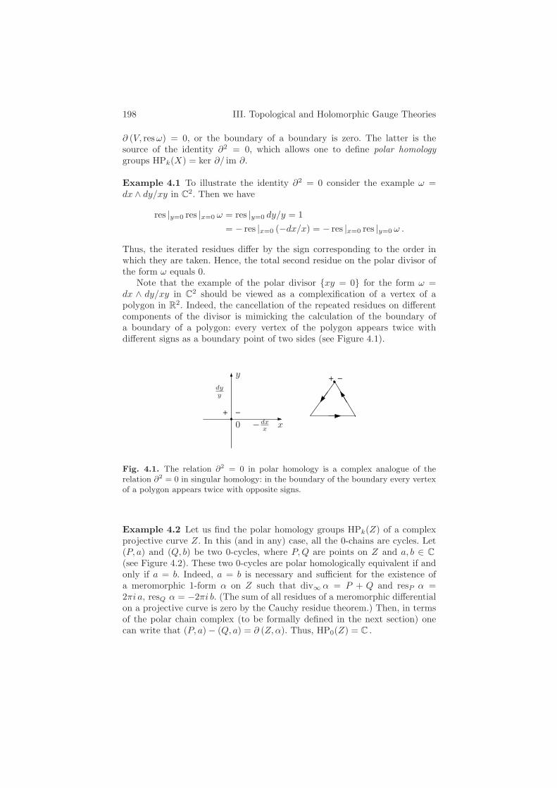
198 III. Topological and Holomorphic Gauge Theories
∂ (V, resω) = 0, or the boundary of a boundary is zero. The latter is thesource of the identity ∂2 = 0, which allows one to define polar homologygroups HPk(X) = ker ∂/ im ∂.
Example 4.1 To illustrate the identity ∂2 = 0 consider the example ω =dx ∧ dy/xy in C
2. Then we have
res |y=0 res |x=0 ω = res |y=0 dy/y = 1= − res |x=0 (−dx/x) = − res |x=0 res |y=0 ω .
Thus, the iterated residues differ by the sign corresponding to the order inwhich they are taken. Hence, the total second residue on the polar divisor ofthe form ω equals 0.
Note that the example of the polar divisor xy = 0 for the form ω =dx ∧ dy/xy in C
2 should be viewed as a complexification of a vertex of apolygon in R
2. Indeed, the cancellation of the repeated residues on differentcomponents of the divisor is mimicking the calculation of the boundary ofa boundary of a polygon: every vertex of the polygon appears twice withdifferent signs as a boundary point of two sides (see Figure 4.1).
+ −
+ −dyy
−dxx0
y
x
Fig. 4.1. The relation ∂2 = 0 in polar homology is a complex analogue of therelation ∂2 = 0 in singular homology: in the boundary of the boundary every vertexof a polygon appears twice with opposite signs.
Example 4.2 Let us find the polar homology groups HPk(Z) of a complexprojective curve Z. In this (and in any) case, all the 0-chains are cycles. Let(P, a) and (Q, b) be two 0-cycles, where P,Q are points on Z and a, b ∈ C
(see Figure 4.2). These two 0-cycles are polar homologically equivalent if andonly if a = b. Indeed, a = b is necessary and sufficient for the existence ofa meromorphic 1-form α on Z such that div∞ α = P + Q and resP α =2πi a, resQ α = −2πi b. (The sum of all residues of a meromorphic differentialon a projective curve is zero by the Cauchy residue theorem.) Then, in termsof the polar chain complex (to be formally defined in the next section) onecan write that (P, a) − (Q, a) = ∂ (Z,α). Thus, HP0(Z) = C .
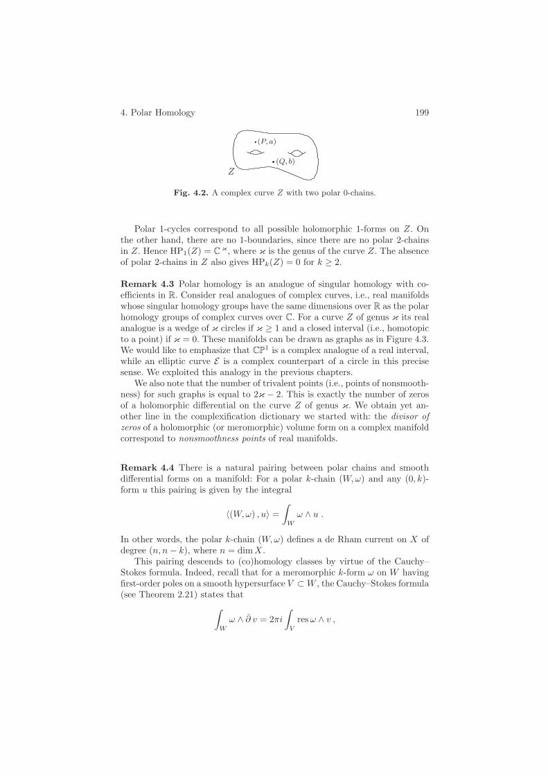
4. Polar Homology 199
Z(Q, b)
(P, a)
Fig. 4.2. A complex curve Z with two polar 0-chains.
Polar 1-cycles correspond to all possible holomorphic 1-forms on Z. Onthe other hand, there are no 1-boundaries, since there are no polar 2-chainsin Z. Hence HP1(Z) = C
κ , where κ is the genus of the curve Z. The absenceof polar 2-chains in Z also gives HPk(Z) = 0 for k ≥ 2.
Remark 4.3 Polar homology is an analogue of singular homology with co-efficients in R. Consider real analogues of complex curves, i.e., real manifoldswhose singular homology groups have the same dimensions over R as the polarhomology groups of complex curves over C. For a curve Z of genus κ its realanalogue is a wedge of κ circles if κ ≥ 1 and a closed interval (i.e., homotopicto a point) if κ = 0. These manifolds can be drawn as graphs as in Figure 4.3.We would like to emphasize that CP
1 is a complex analogue of a real interval,while an elliptic curve E is a complex counterpart of a circle in this precisesense. We exploited this analogy in the previous chapters.
We also note that the number of trivalent points (i.e., points of nonsmooth-ness) for such graphs is equal to 2κ − 2. This is exactly the number of zerosof a holomorphic differential on the curve Z of genus κ. We obtain yet an-other line in the complexification dictionary we started with: the divisor ofzeros of a holomorphic (or meromorphic) volume form on a complex manifoldcorrespond to nonsmoothness points of real manifolds.
Remark 4.4 There is a natural pairing between polar chains and smoothdifferential forms on a manifold: For a polar k-chain (W,ω) and any (0, k)-form u this pairing is given by the integral
〈(W,ω) , u〉 =∫
W
ω ∧ u .
In other words, the polar k-chain (W,ω) defines a de Rham current on X ofdegree (n, n− k), where n = dimX.
This pairing descends to (co)homology classes by virtue of the Cauchy–Stokes formula. Indeed, recall that for a meromorphic k-form ω on W havingfirst-order poles on a smooth hypersurface V ⊂ W , the Cauchy–Stokes formula(see Theorem 2.21) states that
∫
W
ω ∧ ∂ v = 2πi∫
V
resω ∧ v ,

200 III. Topological and Holomorphic Gauge Theories
κ = 0
Z is polar smooth (with po-lar boundary): there exists a1-form with two simple polesand without zeros,
dim HP0(Z) = 1 ,
dim HP1(Z) = 0 .
κ = 1
Z is polar smooth (withouta polar boundary): there ex-ists a 1-form without zerosor poles,
dim HP0(Z) = 1 ,
dim HP1(Z) = 1 .
κ > 1
Z is polar nonsmooth: ageneric holomorphic 1-formhas 2κ − 2 zeros,
dim HP0(Z) = 1 ,
dim HP1(Z) = κ .
Fig. 4.3. The real analogue of a smooth projective curve Z of genus κ.
where v is any smooth (0, k− 1)-form on X. Using the definition of the polarboundary operator, the latter can be rewritten as
〈(W, ω) , ∂v〉 = 〈 ∂(W, ω) , v〉 .
In this way, the Cauchy–Stokes formula defines the pairing between the polarhomology groups of a complex manifold X and the Dolbeault cohomologygroups H0,k
∂(X).
Remark 4.5 One can define polar (k, p)-chains as pairs (A,α), where A ⊂X is a k-dimensional subvariety and α is a meromorphic p-form on A. Therelation ∂2 = 0 still holds in this more general setup, and one obtains polarhomology groups HPk,p. Above, we have been considering the groups HPk =HPk,k. Another interesting case is the case p = 0, in which we consider pairs(A, a), where a ∈ C. Two pairs (A1, a1) and (A2, a2) are equivalent if thereexists a 1-form α on X that has opposite residues on A1 and A2.

4. Polar Homology 201
We also note that the intuitive definition of polar homology above hasto be made more precise, since one cannot restrict to the case of smoothcomplex submanifolds only: the divisor of poles is already not necessarilysmooth. Instead of considering submanifolds, we will define polar chains assmooth varieties along with their maps to our manifold. This is similar tothe definition of singular homology in topology, where one considers maps ofabstract simplices into a manifold. We give a formal definition of the polarhomology groups in the next section. Below we recall the construction of thepushforward of a differential form, which we need for that definition.
Definition 4.6 For a finite covering f : X → Y and a function u on X onecan define its pushforward, or the trace, f∗u as a function on Y whose value ata point is calculated by summing over the preimages taken with multiplicities.The operation f∗ can be generalized to p-forms and to the maps f that areonly generically finite.
Suppose that f : X → Y is a proper, surjective holomorphic mappingwhere both X and Y are smooth complex manifolds of the same dimension n.The pushforward map is a mapping
f∗ : Γ (X,ΩpX) → Γ (Y,Ωp
Y ) .
The pushforward map is also defined for meromorphic forms, f∗ :Γ (X,Mp) → Γ (Y,Mp).
Its construction is as follows. First note that f is generically finite, i.e.,there is an analytic hypersurface D ⊂ Y such that f is a finite unramifiedcovering off this hypersurface D. Hence, for a sufficiently small open neighbor-hood U of any point in Y ∗ := Y D, the inverse image f−1(U) = U1· · ·Ud
is a disjoint union of d open sets Uj , such that f |Ujis an isomorphism with
the inverse sj : U → Uj . Given a form ω on X, one defines its pushforward
f∗ ω := s∗1 ω + · · · + s∗d ω
in U , and therefore in Y ∗. One can check that the form f∗ ω extends acrossthe smooth points of D and hence to the whole of the manifold Y , since theremaining part of D has codimension at least two. The resulting form f∗ ωis holomorphic (respectively, meromorphic) on Y provided the form ω washolomorphic (respectively, meromorphic) on X; see details, e.g., in [149].
Furthermore, the operations of pushforward and residue commute:
Proposition 4.7 Let f : X → Y be a proper surjective holomorphic mapbetween complex manifolds of the same dimension. Let ω be a meromorphicform on X with only first-order poles on a smooth hypersurface V ⊂ X.Suppose that f(V ) is a smooth hypersurface in Y . Then f∗ω has first-orderpoles on f(V ), and
res f∗ω = ˜f∗ resω ,
where ˜f : V → f(V ) is the restriction to V of the map f .
202 III. Topological and Holomorphic Gauge Theories
Example 4.8 To visualize how f∗ω extends across the smooth points of D,consider the following one-dimensional example. Let f : C → C be defined asf : x → y = xm. Then any holomorphic 1-form ω = ψ(x)dx has a holomorphicpushforward 1-form f∗ω = ϕ(y)dy. Indeed, by definition of the pushforward,for any y = 0, we obtain
ϕ(y)dy :=m∑
j=1
ψ(xj) dx =1m
m∑
j=1
xjψ(xj)y
dy ,
where xj are all mth roots of y, and in the last equality we used the relationdy/y = mdx/x for y = xm. This form ϕ(y)dy is well defined for y = 0 and weneed to check that ϕ(y) can be extended to y = 0. Expanding ψ into a powerseries
ψ(x) =∑
l≥0
alxl ,
we obtain
ϕ(y) =1my
m∑
j=1
xjψ(xj) =1my
∑
l≥0
al
m∑
j=1
xl+1j
=1my
∑
k≥1
akm−1(myk) =∑
k≥1
akm−1yk−1 ,
where we have used that∑m
j=1 xnj = 0, unless n = km. This power expansion
in y proves that ϕ(y) is holomorphic at 0, and hence over C.
4.2 Polar Homology of Projective Varieties
In this section we deal with complex projective varieties, i.e., closed subva-rieties of a complex projective space. For a smooth variety X, we denote byΩp
X the sheaf of holomorphic p-forms on X.The space of polar k-chains for a complex projective varietyX of dimension
n is defined as a C-vector space with certain generators and relations.
Definition 4.9 The space of polar k-chains Ck(X) is a vector space over C
defined as the quotient Ck(X) = Ck(X)/Rk, where the vector space Ck(X) isfreely generated by the triples (A, f, α) described in (i), (ii), (iii) and Rk isdefined as relations (R1), (R2), (R3) imposed on the triples:
(i) A is a smooth complex projective variety, dimA = k;(ii) f : A → X is a holomorphic map of projective varieties;(iii) α is a rational k-form on A with first-order poles on V ⊂ A,
where V is a normal crossing divisor in A, i.e., α ∈ Γ (A,ΩkA(V )).
The relations are:

4. Polar Homology 203
(R1) λ(A, f, α) = (A, f, λα) for λ ∈ C .(R2)
∑
i(Ai, fi, αi) = 0 provided that∑
i fi∗αi ≡ 0, where dim fi(Ai) = kfor all i and the pushforwards fi∗αi are considered on the smoothpart of ∪ifi(Ai).
(R3) (A, f, α) = 0 if dim f(A) < k.
Remark 4.10 The relation (R3) implies that Ck(X) = 0 for k > dimX. Alsoby definition, Ck(X) = 0 for k < 0.
The relation (R2) in particular represents additivity with respect to α,that is,
(A, f, α1) + (A, f, α2) = (A, f, α1 + α2).
Here we make no distinction between a triple and its equivalence class. Inparticular, if the polar divisor div∞(α1 + α2) is not normal crossing, one canreplace A by an appropriate blowup, by the Hironaka theorem, where thepullback of α1 + α2 already has a normal crossing polar divisor.
In this way, the relation (R2) allows us to deal with polar chains as pairsreplacing a triple (A, f, α) by a pair (A, α), where A = f(A) ⊂ X, α is definedonly on the smooth part of A and α = f∗α there. Due to the relation (R2),such a pair (A, α) carries precisely the same information as (A, f, α). (Note,however, that such pairs cannot be arbitrary. In fact, by the Hironaka theoremon resolution of singularities, any subvariety A ⊂ X can be the image of someregular A, but the form α on the smooth part of A cannot be arbitrary.)
(A, α)
(V, resV α)
f
( A, α)
X
Fig. 4.4. A polar chain given by the triple (A, f, α) can be thought of as a pair(A, α). Here V = div∞α.
We also note that the consideration of triples (A, f, α) instead of pairs(A, α), which we used in the introduction, is similar to the definition of chainsin singular homology theory. Indeed, in topology one considers the mappingsof abstract simplices into the manifold, but one is interested only in the imagesof simplices. Here also comes a distinction: in contrast to topological homology,where in each dimension k one uses all continuous maps of one standard object(the standard k-simplex or the standard k-cell) to a given topological space,
204 III. Topological and Holomorphic Gauge Theories
in polar homology we deal with complex analytic maps of a large class ofk-dimensional varieties to a given one.
Definition 4.11 The boundary operator ∂ : Ck(X) → Ck−1(X) is defined by
∂(A, f, α) = 2πi∑
i
(Vi, fi, resViα) ,
where Vi are the components of the polar divisor of α, div∞ α = ∪iVi, andthe maps fi = f |Vi
are restrictions of the map f to each component of thedivisor.
Theorem 4.12 ([195]) The boundary operator ∂ is well defined, i.e., it iscompatible with the relations (R1), (R2), and (R3). Furthermore, ∂2 = 0 .
Proof. We have to show that ∂ maps equivalent sums of triples to equivalentones. It is trivial with (R1). For (R2) this follows from the commutativity oftaking residue and pushforward.
To prove the compatibility of ∂ with (R3), consider first the case of apolar 1-chain, a complex curve with a meromorphic 1-form, that is mappedto a point. Then the image of the boundary of this 1-chain is zero. Indeed,this image must be the same point whose coefficient is equal to the sum of allresidues of the meromorphic 1-form on the curve, i.e., zero. The general caseis similar: the same phenomenon occurs along one of the coordinates. (Werefer the interested reader to [195] for more details.)
As to the second part of the statement, we need to prove ∂2 = 0 fortriples (A, f, α) ∈ Ck(X), i.e., for forms α with normal crossing divisorsof poles. The repeated residue at pairwise intersections differs by the signaccording to the order of taking the residues; see Remark 2.22. Thus thecontributions to the repeated residue from different components cancel out(or, equivalently, the residue of a residue is zero).
Definition 4.13 For a smooth complex n-dimensional projective variety X,the chain complex
0 → Cn(X) ∂−→ Cn−1(X) ∂−→ · · · ∂−→ C0(X) → 0
is called the polar chain complex of X. Its homology groups, HPk(X), k =0, . . . , n, are called the polar homology groups of X.
We found in Section 4.1 that the polar homology groups of a complexprojective curve Z of genus κ are HP0(Z) = C and HP1(Z) = C
κ .
Exercise 4.14 Prove that for any n-dimensional X we have HPn(X) =H0(X,Ωn
X) and, if X is connected, also HP0(X) = C .

4. Polar Homology 205
Exercise 4.15 Prove the functoriality of polar homology, i.e., that a regularmorphism of projective varieties h : X → Y defines a homomorphism h∗ :HPk(X) → HPk(Y ).
After the formal definitions have been given, we would like to show whythe Dolbeault complex of (0, k)-forms should be related to the polar homol-ogy in the same way as the de Rham complex of smooth forms is related tothe singular homology. First we show how the space of polar chains Ck(X)for a smooth projective variety X can be viewed as a subspace of currents,functionals on smooth differential forms on X.
Definition 4.16 A polar k-chain represented by a triple a = (A, f, α) definesthe following linear functional on smooth (0, k)-forms. Its value on a smooth(0, k)-form u on X is given by the pairing
〈a , u〉 :=∫
A
α ∧ f∗u . (4.9)
The integral is well defined, since the meromorphic k-form α has only first-order poles on a normal crossing divisor.
Remark 4.17 It is straightforward to show that the pairing 〈 , 〉 descends tothe space Ck(X) of equivalence classes of triples, i.e., that it is compatible withthe relations (R1), (R2), (R3) of Definition 4.9. Indeed, (R1) is obvious, thecompatibility with (R3) is a consequence of the equality f∗u = 0 if dim f(A) <k, and the compatibility with (R2) follows from the relation
∫
Aα ∧ f∗u =
∫
f(A)f∗α∧u if dim f(A) = k, where the last integral is taken over the smooth
part of f(A).
Proposition 4.18 The pairing (4.9) defines the following homomorphism in(co)homology:
ρ : HPk(X) → Hn,n−k
∂,
where n = dimX.
Proof. By Serre duality, ρ is a map HPk(X) → (H0,k
∂(X))∗, and it is
sufficient to verify that the pairing vanishes if ∂a = 0 and u = ∂v, or if∂u = 0 and a = ∂b. This follows immediately from the Cauchy–Stokes formula(Theorem 2.21):
∫
A
α ∧ f∗(∂u) = 2πi∫
div∞ α
(resα) ∧ f∗(u) ,
that is, 〈a , ∂u〉 = 〈∂a , u〉.
One can prove that for smooth projective manifolds the homomorphism ρis in fact an isomorphism:
206 III. Topological and Holomorphic Gauge Theories
Theorem 4.19 (Polar de Rham Theorem, [197]) For a smooth projec-tive manifold X the map ρ : HPk(X) → Hn,n−k
∂is an isomorphism of the polar
homology and Dolbeault cohomology groups. Equivalently, HPk(X) ∼= H0,k
∂(X)
in terms of dual cohomology groups.
Example 4.20 For a complex curve Z of genus κ one has HP0(Z) ∼= C ∼=H1,1
∂(Z) and HP1(Z) ∼= C
κ ∼= H1,0
∂(Z).
Remark 4.21 As we mentioned in the introduction, one could consider moregeneral polar (k, p)-chains (A, f, α), where α is a meromorphic p-form on Aof not necessarily maximal degree, p k, that can have only logarithmic sin-gularities on a normal crossing divisor. The requirement of log-singularities isneeded to have a convenient definition of the residue and hence the boundaryoperator ∂. The Cauchy–Stokes formula, the property ∂2 = 0, and the def-inition of the polar homology groups HPk,p(M) can be carried over to this,more general, situation.
As a consequence, the natural pairing between polar (k, p)-chains andsmooth (k − p, k)-forms on X gives us the homomorphism
ρ : HPk,p(X) → Hn−k+p,n−k
∂(X) .
However, unlike the case p = k, the map ρ is not, in general, an isomorphismfor other values of p, 0 p < k. For instance, in the case of p = 0, theimage consists of algebraic k-cycles (tensored with C), while the full spaceHn−k,n−k
∂(X) can be much larger. It would be interesting to find an ad-
justment of the groups HPk,p(M) to provide the isomorphism and hence toobtain a description of the chain complex for the Dolbeault cochains in alldimensions.
4.3 Polar Intersections and Linkings
We start by defining a polar analogue for the topological intersection number.Recall that in topology one considers a smooth oriented closed manifoldM andtwo oriented closed submanifolds A,B ⊂ M of complementary dimensions,i.e., dimA + dimB = dimM . Suppose A and B intersect transversally at afinite number of points. Then to each intersection point P one assigns thelocal intersection index equal to ±1 by comparing the mutual orientations ofthe tangent vector spaces TPA, TPB, and TPM .
Now let X be a complex compact manifold of dimension n equipped witha nowhere-vanishing holomorphic n-form µ. Such a pair (X,µ) can be thoughtof as a polar analogue of an oriented closed manifold. (Recall that if µ werenonvanishing and meromorphic with first-order poles, this would be a polaranalogue of an oriented manifold with boundary, while zeros of the n-form µcould be regarded as a complex analogue of singularities of a real manifold.)

4. Polar Homology 207
Note that the existence of such a form requires the canonical bundle of thecomplex manifold X to be trivial, i.e., X can be a Calabi–Yau manifold, anabelian one, or a product of such.
Definition 4.22 Consider two polar cycles (A,α) and (B, β) of complemen-tary dimensions that intersect transversally in the polar oriented complexmanifold (X,µ). The polar intersection number of the cycles (A,α) and (B, β)is given by the following sum over the set of points in A ∩B:
(A,α) · (B, β) =∑
P∈A∩B
α(P ) ∧ β(P )µ(P )
.
Here α(P ) and β(P ) are understood as exterior forms on TPM = TPA×TPBobtained by the pullback from the corresponding factors.
Remark 4.23 At every intersection point P , the ratio in the right-hand sidecan be regarded as the comparison of the polar orientations of the cycles atthat point with the orientation of the ambient manifold. Note that in thepolar case, the intersection number does not have to be an integer. Rather, itshould be viewed as a function of the “parameters” (A,α), (B, β), and (X,µ).
Remark 4.24 Essentially the same formula defines the intersection productof transversal polar cycles when they intersect over a manifold of positivedimension. Namely, for polar cycles (A,α) and (B, β) of dimensions p and qsuch that p+ q ≥ n and transversal to each other, their intersection is a polar(p+q−n)-cycle (C, γ) := (A,α) ·(B, β), where C = A∩B and γ := (α ∧ β)/µ.In this way, one obtains the map
HPp(M) ⊗ HPq(M) → HPp+q−n(M) ,
upon finding smooth transverse representatives for every pair of homologyclasses. This map is well defined, as follows from the polar de Rham theorem;see [194] for more details.
Exercise 4.25 Check that the (p+ q− n)-form γ = (α ∧ β)/µ is indeed welldefined on the complex manifold C. (Hint: this is a problem in linear algebra.)
A similar construction allows one to define a polar analogue of a linkingnumber. Recall that the Gauss linking number of two oriented closed curvesin R
3 is an integer topological invariant equal to the algebraic number ofcrossings of one curve with a two-dimensional oriented surface bounded bythe other curve; see Section 3.4. The linking number is a homology invariantin the following sense: it does not change if one of the curves is replacedby a homologically equivalent cycle in the complement to the other curve.More generally, the linking number can be defined for two oriented closed
208 III. Topological and Holomorphic Gauge Theories
submanifolds of linking dimensions in any oriented (but not necessarily simplyconnected) manifold, provided that both submanifolds are homologous to zero.
To define the polar linking number we will “translate” the classical def-inition into the polar language. Let (A,α) and (B, β) be two polar smoothnonintersecting cycles of dimensions p and q in a polar oriented closed n-manifold (M,µ). Suppose that these cycles are polar boundaries (i.e., theyare polar homologous to 0) and are of linking dimensions: p+ q = n− 1.
Definition 4.26 The polar linking number of cycles (A,α) and (B, β) in(M,µ) is
lkpol ((A,α), (B, β)) :=∑
P∈A∩S
α(P ) ∧ σ(P )µ(P )
,
where a chain (S, σ) has the polar boundary (B, β) = ∂(S, σ). In other words,lkpol ((A,α), (B, β)) is the intersection of the polar cycle (A,α) and the polarchain (S, σ), provided they intersect transversely.
Theorem 4.27 ([195, 196]) The polar linking number lkpol((A,α), (B, β))is
(i) well defined, i.e., lkpol does not depend on the choice of the polar chain(S, σ), provided that ∂(S, σ) = (B, β);
(ii) (anti-)symmetric:
lkpol ((A,α), (B, β)) = (−1)(n−p)(n−q) lkpol ((B, β), (A,α)) ;
(iii) invariant when (A,α) is replaced by a cycle (A′, α′) polar homologousto (A,α) in the complement of B ⊂ X.
Remark 4.28 In particular, for p = q = 1 we have defined a polar linking ofcomplex curves in a complex threefold, all equipped with volume forms. Thepolar linking number is symmetric in this dimension. The simplest curvesthat can have nontrivial linking are elliptic curves: the linking number of arational curve with any other curve is zero, since any holomorphic differentialon a rational curve must vanish.
Exactly this polar linking number of complex curves appears from theholomorphic abelian Chern–Simons path integral, in the same way as the usuallinking number comes out of the topological Chern–Simons path integral (seeSection 3.4 and [134, 195, 366]).
The polar linking number is also closely related to the Weil pairing of func-tions on a complex curve and to the Parshin symbols, the higher-dimensionalgeneralizations of the latter; see [309]. One intriguing open question in thearea is to find a polar analogue of the self-linking number of a framed knot.

4. Polar Homology 209
4.4 Polar Homology for Affine Curves
So far, we have studied polar homology of projective varieties, which play therole of compact manifolds in usual topology. It is natural to expect that therole of noncompact manifolds should be played by quasi-projective varieties,i.e., Zariski open subsets in projective varieties. In this section, following [195],we indicate how the polar homology theory can be extended to affine curves,one-dimensional quasi-projective varieties.
Let X be an affine curve and let X be its projective closure, i.e., X isZariski open in X. Denote by D := X X the compactification divisor. Weshall define the polar chains for the quasi-projective variety X as a certainsubset of polar chains for X.
Definition 4.29 The space Ck(X) of polar k-chains in X is defined as thesubspace in Ck(X) such that the corresponding k-forms vanish on D:
Ck(X) = (A, f, α) ∈ Ck(X) | α(x) = 0 for all x ∈ f−1(D) ⊂ A .
In particular, for an affine curve X the space C0(X) of polar 0-chains isthe vector space formed by complex linear combinations of points in X, whilefor C1(X) we consider smooth projective curves A and logarithmic 1-forms αthat vanish at f−1(D) ⊂ A.
Definition / Proposition 4.30 For the affine curve X the spacesCk(X), k = 0, 1, form a subcomplex in the polar chain complex (C•(X), ∂),which depends only on X and not on the choice of its compactification, theprojective curve X.
The resulting homology groups of the chain complex (C•(X), ∂) are denoted,as before, by HPk(X) and are called polar homology groups of X.
Example 4.31 Consider the case X = X \ P of a smooth projective curveof genus κ with one point removed. Then dim HP1(X) = κ − 1 if κ ≥ 1and dim HP1(X) = 0 if κ = 0. Indeed, the space HP1(X) is the space ofholomorphic 1-forms on X that vanish at P .
To calculate HP0(X) in the case κ ≥ 1 it is sufficient to notice that for anytwo points Q1, Q2 ∈ X \ P, the 0-cycle (Q1, q1) + (Q2, q2) is homologicallyequivalent to zero if and only if q1 + q2 = 0 (the same condition as in thecase of a nonpunctured curve, which we discussed in the introduction). In thecase of κ = 0 an analogous statement requires three points to be involved(unlike the case of a nonpunctured projective line): the corresponding 1-formon CP
1 has to have at least one zero, and hence at least three poles. Hencedim HP0(X) = 1 if κ ≥ 1 and dim HP0(X) = 2 if κ = 0.
We collect the results about the curves in Figure 4.5, where we depictthe complex curves by graphs such that polar homology groups of the curvescoincide with singular homology groups of the corresponding graphs.

210 III. Topological and Holomorphic Gauge Theories
This way the divisor of zeros of a meromorphic form becomes a counter-part of punctures (or infinity) in an open real manifold. (Recall that in theintroduction we also observed that the divisor of zeros can also stand for thepoints of nonsmoothness. These two points of view are consistent, since onecan “puncture” a closed singular real variety at its singularities and make itsmooth, but open.)
κ = 0
dim HP0(X) = 2 ,
dim HP1(X) = 0 .
κ = 1
dim HP0(X) = 1 ,
dim HP1(X) = 0 .
κ > 1
dim HP0(X) = 1 ,
dim HP1(X) = κ − 1 .
Fig. 4.5. A smooth projective curve with one point removed, X = X P.
Example 4.32 In a similar way, one can deal with the case X = X P,Qof a smooth projective curve with two points removed. We summarize theresults in Figure 4.6. Here, one has to distinguish between the case of genericpoints P and Q and the case that P +Q is a special divisor. In the latter casethere exist more 1-differentials with zeros at P,Q than generically.
The consistency of the definitions of polar homology in the projective andquasi-projective cases is provided by the following Mayer–Vietoris sequence:the corresponding groups behave like ordinary homology groups with respectto taking unions of Zariski open subsets in the curve X.
Theorem 4.33 Let a complex curve X = U1 ∪ U2 (either affine or projec-tive) be the union of two Zariski open subsets U1 and U2 . Then the followingMayer–Vietoris sequence of chains is exact:
0 → Ck(U1 ∩ U2)i−→ Ck(U1) ⊕ Ck(U2)
σ−→ Ck(X) → 0.
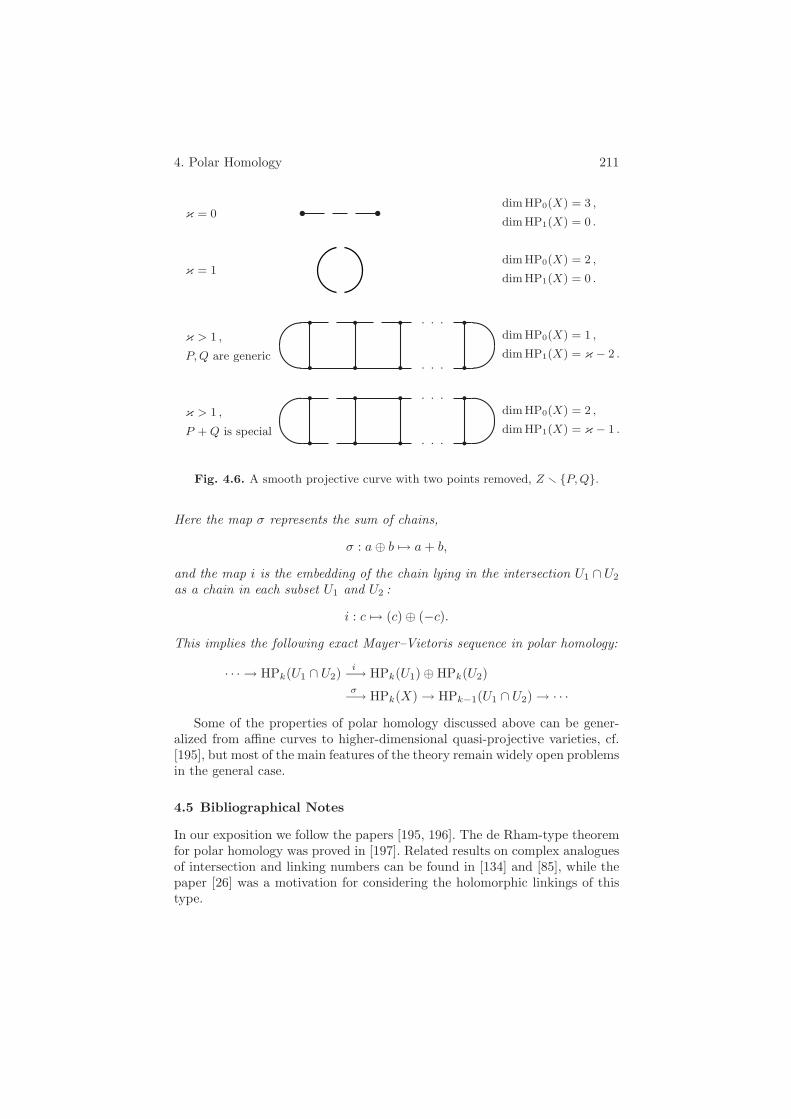
4. Polar Homology 211
κ = 0
κ = 1
κ > 1 ,
P, Q are generic
κ > 1 ,
P + Q is special
dim HP0(X) = 3 ,
dim HP1(X) = 0 .
dim HP0(X) = 2 ,
dim HP1(X) = 0 .
dim HP0(X) = 1 ,
dim HP1(X) = κ − 2 .
dim HP0(X) = 2 ,
dim HP1(X) = κ − 1 .
Fig. 4.6. A smooth projective curve with two points removed, Z P, Q.
Here the map σ represents the sum of chains,
σ : a⊕ b → a+ b,
and the map i is the embedding of the chain lying in the intersection U1 ∩ U2
as a chain in each subset U1 and U2 :
i : c → (c) ⊕ (−c).
This implies the following exact Mayer–Vietoris sequence in polar homology:
· · · → HPk(U1 ∩ U2)i−→ HPk(U1) ⊕ HPk(U2)σ−→ HPk(X) → HPk−1(U1 ∩ U2) → · · ·
Some of the properties of polar homology discussed above can be gener-alized from affine curves to higher-dimensional quasi-projective varieties, cf.[195], but most of the main features of the theory remain widely open problemsin the general case.
4.5 Bibliographical Notes
In our exposition we follow the papers [195, 196]. The de Rham-type theoremfor polar homology was proved in [197]. Related results on complex analoguesof intersection and linking numbers can be found in [134] and [85], while thepaper [26] was a motivation for considering the holomorphic linkings of thistype.

212 III. Topological and Holomorphic Gauge Theories
The definition of polar chains and the boundary operator has similar fea-tures with Abel’s theorem [149] and with Ishida’s complexes for toric varieties[296].
For a thorough treatment of logarithmic forms see [78], while for multidi-mensional residues we refer the reader to the detailed monograph [369]; seealso [150].
The term “polar homology” was coined in [195], and it originated fromconsideration of polar divisors of differential forms. One may think that thelaunch of the Antarctica Journal of Mathematics in 2004, soon after the ap-pearance of the polar theory, was not a simple coincidence.

Appendices
A.1 Root Systems
1.1 Finite Root Systems
Let V be a finite-dimensional real vector space and let ( , ) be a positivedefinite symmetric bilinear form on V . For an element α ∈ V we denote byrα the reflection in the hyperplane orthogonal to α:
rα(β) = β − 2(β, α)(α, α)
α
for any point β ∈ V .
Definition 1.1 A subset R of V is called a (finite) root system if the followingaxioms are satisfied:
(R1a) The set R is finite and it spans the vector space V .(R1b) 0 ∈ R .(R2) For any α ∈ R the reflection rα maps the set R to itself.(R3) If α, β ∈ R, then 2(β, α)/(α, α) ∈ Z.(R4) If α ∈ R, then 2α ∈ R.14
The elements of a root system R are called roots. Two root systems R and R′
are called isomorphic if there exists an isomorphism ϕ of the correspondingvector spaces V and V ′ mapping R to R′ and such that
(ϕ(β), ϕ(α))/(ϕ(α), ϕ(α)) = (β, α)/(α, α)
for all α , β ∈ R.14 Sometimes this is called a reduced root system, as opposed to a nonreduced one,
for which the axiom (R4) is dropped.

214 Appendices
Definition 1.2 A root system R is called irreducible if it cannot be decom-posed into two nonempty subsets R1 and R2 such that R1 is orthogonal toR2 and R = R1 ∪R2.
Axioms (R2) and (R3) restrict the relative lengths of and the angles be-tween the roots. For example, in an irreducible root system, only roots oftwo different lengths can occur, and they are called the short and long rootsrespectively. Irreducible root systems can be classified. There are four infiniteseries (the root systems of types An, Bn, Cn, Dn) and five exceptional rootsystems (the root systems of types E6, E7, E8, F4, and G2). Here the indexdenotes the dimension of the ambient vector space V . Figure 1.1 shows alltwo-dimensional root systems (note that the root system of type A1×A1 isnot irreducible).
B2∼=C2A1×A1 A2 G2
Fig. 1.1. The two-dimensional root systems.
Definition 1.3 Let R ⊂ V be a root system. The subgroup W ⊂ GL(V )generated by the reflections rα for all α ∈ R is called the Weyl group of theroot system R.
Definition 1.4 A subset Π ⊂ R of a root system R ⊂ V is called a basis ofR if Π is a basis of the vector space V and if every element β ∈ R can beexpressed as β =
∑
α∈Π mαα such that either all mα are nonnegative integersor all mα are nonpositive integers.
Proposition 1.5 Every root system has a basis. For a given root system R,the Weyl group of R permutes the set of all bases of R.
After having fixed a basis Π of the root system R, we can decompose R intoR = R+ ∪R−, where R+ = β ∈ R |β =
∑
α∈Π mαα with mα ≥ 0 is the setof positive roots of R and R− = −R+ is the set of negative roots of R.
Example 1.6 Let V = x = (x1, . . . , xn+1) ∈ Rn+1 |x1 + · · · + xn+1 = 0
with the inner product induced from the standard inner product on Rn+1.
Then the set

A.1. Root Systems 215
R = x ∈ Zn+1 |x ∈ V and (x, x) = 2
is a root system of type An. The Weyl group of this root system is given bythe symmetric group Sn+1, which acts on the entries of the vectors in V bypermutation. A basis of R is given by the set Π = e1−e2, e2−e3, . . . , en−1−en, where the vector ei = (0, . . . , 0, 1, 0, . . . , 0) has 1 at the ith entry and 0’severywhere else.
1.2 Semisimple Complex Lie Algebras
Here we shall briefly indicate how the finite root systems appear in the theoryof semisimple Lie algebras.
Definition 1.7 A nonabelian Lie algebra g is called simple if it does nothave any nonzero ideals other than g itself. A finite-dimensional semisimpleLie algebra g is a direct sum of nonabelian simple Lie algebras; cf. DefinitionI.1.31.
Let g be a complex finite-dimensional semisimple Lie algebra, and let h ⊂ g
be its Cartan subalgebra, that is, a maximal abelian subalgebra all of whoseelements are diagonalizable by the adjoint action. Such subalgebras exist fordimensional reasons. Since the elements of h commute, one can diagonalizetheir adjoint action on g simultaneously. The latter allows one to write
g =⊕
α∈h∗
gα (1.10)
withgα = X ∈ g | [H,X] = α(H)X for all H ∈ h .
One can show that g0 = h and that for α = 0, each nonzero gα is one-dimensional. The set R of all α ∈ h∗ with α = 0 and gα = 0 is called theroot system of the Lie algebra g. Hence, decomposition (1.10) is, in fact, asfollows:
g = h ⊕⊕
α∈R
gα . (1.11)
It is called the root space decomposition of the semisimple Lie algebra g.
Example 1.8 For the Lie algebra sl(2,C) the root space decomposition is asfollows:
sl(2,C) = 〈e〉 ⊕ 〈h〉 ⊕ 〈f〉.Here the Cartan subalgebra h = 〈h〉 is one-dimensional, and the two rootscorresponding to the subspaces 〈e〉 and 〈f〉 are opposite in sign: [h, e] = 2h =−[h, f ] and [e, f ] = h.
216 Appendices
It turns out that the root system R is a finite root system in the sense ofDefinition 1.1. Furthermore, the root system R of the Lie algebra g determinesthe semisimple Lie algebra g up to an isomorphism: given a root system R,one can construct a finite-dimensional complex semisimple Lie algebra g withthis root system. Finally, the Lie algebra g is simple exactly if its root systemis irreducible. So there is a one-to-one correspondence between complex finite-dimensional simple Lie algebras and irreducible root systems of types An, Bn,Cn, Dn, E6, E7, E8, F4, and G2.
Example 1.9 Consider the Lie algebra g = sl(n+ 1,C) with the Cartansubalgebra of diagonal matrices. For i = j we define αij ∈ h∗ byαij(diag(q1, . . . , qn)) = qi − qj . Furthermore, let gαij
denote the subspacespanned by the matrix with 1 at the (i, j)th entry and 0’s everywhere else.Then the root space decomposition of the Lie algebra sl(n+ 1,C) is given by
sl(n+ 1,C) = h ⊕⊕
αij∈R
gαij,
where the root system R is of type An.The root system of type Bn corresponds to the Lie algebra so(2n+ 1,C),
the root system Cn is related to the Lie algebra sp(2n,C), while Dn corre-sponds to the algebra so(2n,C).
1.3 Affine and Elliptic Root Systems
Let V be a real finite-dimensional vector space with a positive semidefinitesymmetric bilinear form ( , ) and let α ∈ V be a vector for which (α, α) = 0.Similarly to the positive definite case, the reflection rα can be defined via
rα(β) := β − 2(α, β)(α, α)
α .
Definition 1.10 A subset R ⊂ V is called an extended root system if Rsatisfies the following axioms:
(ER1a) The additive subgroup Q(R) =∑
α∈R Zα is a full lattice in V .(ER1b) (α, α) = 0 for all α ∈ R .(ER2) For any α ∈ R the reflection rα maps the set R to itself.(ER3) If α, β ∈ R, then 2(β, α)/(α, α) ∈ Z.(ER4) If α ∈ R, then 2α ∈ R.
An extended root system R is called irreducible if it cannot be decomposedinto two nonempty subsets R1 and R2 such that (R1, R2) = 0.
Axiom (ER1) means that the set Q(R) is the Z-span of an R-basis of V ,being an analogue of axiom (R1). For finite root systems, the fact that theset Q(R) is a lattice in V is Proposition 1.5. Note, however, that unless the

A.1. Root Systems 217
bilinear form on V is positive definite, the extended affine root systems arenever finite.
Let R be an extended root system. The dimension of the radical
V0 = v ∈ V | (v, w) = 0 for all w ∈ V
is called the nullity of the root system R. It turns out that the extended rootsystems of nullity 0 are exactly the finite root systems. Other extended rootsystems playing a role in this book are those of nullity 1 and 2.
Definition 1.11 An irreducible extended root system of nullity 1 is called anaffine root system. An extended root system of nullity 2 is called an ellipticroot system.
Remark 1.12 We note that no isotropic roots are allowed in R. Our defini-tion of extended root systems is taken from [334]. In the literature there existsanother definition for extended root systems that includes isotropic roots (see,e.g., [8]), which is shown to be equivalent to the one above; see [30].
The Weyl groups for affine and elliptic root systems are defined in thesame way as the Weyl groups for finite root systems.
Taking the quotient of an affine root system by the radical of the bilinearform gives a (possibly nonreduced) finite root system. Hence, one can attemptto classify affine root systems in terms of the underlying finite root systems.The full list of irreducible affine root systems up to isomorphism is A(1)
n , B(1)n ,
C(1)n , D(1)
n , E(1)6 , E(1)
7 , E(1)8 , F(1)
4 , G(1)2 , A(2)
2n+1, A(2)2n , D(2)
n , E(2)6 , E(2)
7 , D(3)4 . (Here,
the notation for the root systems is the same as in [178].) The root systems oftype X(1)
n are called untwisted affine root systems; the systems of type X(r)n
with r > 1 are called twisted affine root systems.
Example 1.13 The untwisted affine root systems can be easily constructedfrom the corresponding finite root systems: Let R ⊂ V be a finite root systemof type Xn (for example, the root system of type An from Example 1.6).Extend the bilinear form ( , ) trivially from V to the space ˜V = V ⊕R. Thenthe set
˜R = (α, n) ∈ ˜V |α ∈ R and n ∈ Z
is an affine root system of type X(1)n . The construction of the twisted affine
root systems is more complicated (see, e.g., [178]).
In the theory of loop groups and affine Lie algebras, the affine root systemsplay a role similar to that of the finite root systems in the theory of compactLie groups and semisimple Lie algebras.
218 Appendices
Example 1.14 Let g be the Lie algebra sl(n+ 1,C) and let h ⊂ g denote theCartan subalgebra of diagonal matrices. Consider the corresponding affine Liealgebra ˜Lg (or, rather, (˜Lg)pol) whose underlying vector space is given by
˜Lg = g ⊗ C[z, z−1] ⊕ Cω ⊕ Cd ;
cf. Remark II.1.14. The Lie bracket on ˜Lg is given by
[ω,X(z)] = [ω, d] = 0, [d,X(z)] = zd
dzX(z),
and
[X(z), Y (z)] = [X,Y ](z) +1
2πi
(
∫
|z|=1
⟨
X(z),d
dzY (z)
⟩
dz
)
· ω .
Here [X,Y ](z) denotes the pointwise commutator of X and Y , and 〈 , 〉 is thenormalized Killing form on g. Now set ˜h := h⊕Cω⊕Cd and choose an elementδ ∈ (h⊕Cω⊕Cd)∗ dual to the basis element d, i.e., such that δ(d) = 1, δ(ω) =0 and δ(X) = 0 for all X ∈ h. Then the set ˜R = α+mδ | α ∈ R, m ∈ Z isan affine root system of type A(1)
n for the Lie algebra ˜Lg. In order to write outa root space decomposition for this Lie algebra ˜Lg, it is convenient to use thenotion of an extended root system that includes isotropic roots; see details in[178, 8].
Remark 1.15 The elliptic root systems can be classified in a way similar toaffine root systems in terms of the underlying finite root systems (see [8], [334])and they play a similar role in the theory of double loop algebras (elliptic orextended affine algebras) and double loop groups. Namely, consider the space˜
˜V := V ⊕ R ⊕ R with the bilinear form ( , ) extended trivially and a finiteroot system R ⊂ V . Then the set
˜
˜R = (α, n,m) ∈ ˜
˜V |α ∈ R and n,m ∈ Z
is an elliptic root system, usually denoted by X(1,1)n .
Exercise 1.16 Find a root space decomposition of the sl(2,C)-elliptic Liealgebra introduced in Definition II.5.1 of Chapter II.
1.4 Root Systems and Calogero–Moser Hamiltonians
In Section II.5.4 we considered a system of n interacting particles moving onthe real line and governed by the Hamiltonian function
H(q1, . . . , qn, p1, . . . , pn) =12
n∑
i=1
p2i +
∑
i>j
U(qi − qj) , (1.12)

A.1. Root Systems 219
where the coordinates qi denote the positions of the particles and pi denotetheir momenta. We looked at the potentials of the form U(ξ) = 1/ξ2 (therational potential), U(ξ) = 1/ sin2 ξ or U(ξ) = 1/ sinh2 ξ (the trigonomet-ric/hyperbolic potential), and, finally, the elliptic potentials U(ξ) = ℘(ξ; τ),where ℘( . , τ) denotes the Weierstrass ℘-function with the periods 1 and τ .
It has been observed in [298] that the Hamiltonian (1.12) can be general-ized to the Hamiltonian
H(q, p) =12(p, p) +
12
∑
α∈R
m|α|U(α(q)) , (1.13)
where R ⊂ V is any finite root system in the vector space V with innerproduct ( , ), and m|α| is a constant that depends only on the length of theroot α. The momentum vector p is an element of the vector space V , and theposition q is an element of the dual space V ∗. The Hamiltonian systems (1.13)are integrable for any finite irreducible root system R [298, 50].
Here we would like to stress the fact that the three types of Hamiltonians(rational, trigonometric, and elliptic) are naturally related to the three typesof root systems (finite, affine, and elliptic) considered in this section. Indeed,consider, for instance, the elliptic case. Let R ⊂ V be an elliptic root system,and let V ∗ denote the dual space of the finite-dimensional vector space V . Theradical V0 of the bilinear form ( , ) has dimV0 = 2 in the elliptic case. Uponchoosing a decomposition V ∗ = h ⊕ V ∗
0 one can denote elements of the spaceV ∗ by triples (q, a, b), where q ∈ h and (a, b) ∈ V ∗
0 . Now we can write downthe potential on h corresponding to the elliptic root system R as follows:
U(q) =12
∑
α∈R
(
1(α(q, 1, τ))2
− 1(α(0, 1, τ))2
)
(1.14)
for some fixed τ ∈ C with Im τ > 0. Note that for the root system of typeA
(1,1)n−1 from Example 1.15, the potential U defined by the expression (1.14) can
be rewritten via the Weierstrass ℘-function and coincides with the potentialof the standard elliptic Calogero–Moser system. Using the classification ofirreducible elliptic root systems, one shows that the potential (1.14) defines aholomorphic function on the complexified vector space h ⊗ C. It is known formany elliptic root systems (and, apparently, is the case for all of them) thatthe corresponding Hamiltonian systems are integrable [51].
Exercise 1.17 Write down the potential U for the affine root system A(1)n−1
and verify that it coincides with the potential of the trigonometric Calogero–Moser system.
More facts on root systems can be found in [56] and [168]. The latter isalso a good reference for finite-dimensional semisimple complex Lie algebras.For the affine root systems and Lie algebras we refer the reader to [178], whilethe extended root systems of higher nullity (and, in particular, the elliptic

220 Appendices
ones), along with the corresponding Lie algebras, have been studied in [8] and[334].
A.2. Compact Lie Groups 221
A.2 Compact Lie Groups
In this appendix we recall some basic facts from the theory of compact Liegroups (see, e.g., [60] for more details and references). Throughout this section,G denotes a finite-dimensional compact connected Lie group with the Liealgebra g. The compact Lie groups that are abelian are the easiest ones todescribe. Indeed, any n-dimensional compact connected abelian Lie group isisomorphic to the torus T = R
n/Zn. The other extreme is formed by simpleLie groups.
2.1 The Structure of Compact Groups
Definition 2.1 A compact connected Lie group G is called semisimple if itscenter is finite. The group G (of dim > 1) is called simple if it does not haveany nontrivial normal connected subgroups.
Recall that any Lie group G acts on its Lie algebra by the adjoint repre-sentation. If the group G is compact there exists a negative definite invariantsymmetric bilinear form on the Lie algebra g. This form is, in general, notunique.
Definition / Proposition 2.2 If the compact Lie group G is simple, thereexists a unique (up to a scalar factor) symmetric and negative definite invari-ant bilinear form on its Lie algebra g, called the Killing form.
Remark 2.3 For a finite-dimensional Lie algebra g, the Killing form is de-fined as 〈X,Y 〉 := tr(adX adY ). The Cartan criterion states that the Killingform is nondegenerate exactly when the Lie algebra g is semisimple. If g issimple then any invariant symmetric bilinear form on g is a scalar multiple ofthe Killing form. Furthermore, the Lie algebra g corresponds to a compact Liegroup exactly if the Killing form 〈X,Y 〉 := tr(adX adY ) is negative definite.For matrix Lie algebras this form is a multiple of the trace form tr(XY ). Formost purposes in this book we use the trace version of the form. Often it isconvenient to change the sign and think of the positive definite Killing form(see, for example, the discussion of roots in Appendix A.1, where the Killingform is used to measure length of the roots).
Example 2.4 The group SU(n) is simple. Its center is isomorphic to thecyclic group Z/nZ. The Killing form 〈X,Y 〉 := tr(adX adY ) on the Liealgebra su(n) is given by the trace: 〈X,Y 〉 = − tr(XY ).
The importance of simple compact groups is clear from the following struc-ture theorem.

222 Appendices
Theorem 2.5 Let G be a compact connected Lie group. Then G is isomorphicto an “almost direct product”
G ∼= (G1 × · · · ×Gk × T ) /Z ,
where the Gi are simply connected simple Lie groups, T is a compact connectedabelian Lie group (i.e., a torus), and Z is a finite subgroup of the center ofG1 × · · · × Gk × T . In particular, every simply connected compact Lie groupis a direct product of simply connected simple Lie groups.
An important role in the theory of compact Lie groups is played by certainabelian subgroups: a maximal torus of the compact connected Lie group G isa maximal connected abelian subgroup T ⊂ G. For dimensional reasons, max-imal tori exist. Furthermore, one can show that every element of a compactconnected Lie group G is contained in some maximal torus of G.
Theorem 2.6 Any two maximal tori of a compact connected Lie group G areconjugate in G. In particular, every element of the group G is conjugate to anelement inside a fixed maximal torus T ⊂ G.
The exponential map for compact tori is surjective. Together with Theorem2.6 this observation implies the following corollary.
Corollary 2.7 For any compact connected Lie group G the exponential mapexp : g → G is surjective.
Definition / Proposition 2.8 Let T ⊂ G be a maximal torus, and denoteby N(T ) its normalizer in G, i.e., the elements of G that conjugate T to itself.Then the group W (T ) = N(T )/T is a finite group, called the Weyl group ofG with respect to T .
Theorem 2.9 Let T ⊂ G be a maximal torus of G. Then two elements t, t′ ∈T are conjugate under G if and only if they are conjugate under W (T ). Inparticular, the set of conjugacy classes of a compact connected Lie group Gcan be identified with the set T/W (T ).
The quotient T/W (T ) is called the fundamental alcove of the group G.
Example 2.10 A maximal torus T of the group G = SU(n) is given by theset of diagonal matrices. So in this case, Theorem 2.6 is merely a reformulationof the fact that every element of the group SU(n) is diagonalizable. The Weylgroup W (T ) of SU(n) is isomorphic to the symmetric group Sn, which actson the torus T by permuting the elements on the diagonal. Thus, definingt := diag(e2πia1 , . . . , e2πian), we can identify the set of conjugacy classes T/Sn
with the set (a1, . . . , an) ∈ Rn | a1 ≥ · · · ≥ an,
∑
ai = 0 and a1 − an ≤ 1.
A.2. Compact Lie Groups 223
Our next goal is to describe the fundamental group of the compact Liegroup G. In view of Theorem 2.5, it is enough to consider the case of a semi-simple group G. First we sidestep slightly and introduce the root lattice of G.Let us fix a maximal torus T ⊂ G, and denote its Lie algebra by h; cf. Appen-dix A.1. (The latter is called a Cartan subalgebra of the Lie algebra g.) Recallthat the group G acts on its Lie algebra g and hence on the complexificationg ⊗ C by the adjoint action. Since the maximal torus T ⊂ G is an abeliangroup, we can simultaneously diagonalize its action on the complexified Liealgebra g ⊗ C. This allows one to decompose the vector space g ⊗ C into
g ⊗ C =⊕
α∈h∗
gα ,
where gα denotes the space
gα = X ∈ g ⊗ C | [H,X] = α(H)X for all H ∈ h .
Here the nonzero elements 0 = α ∈ h∗ of the dual Cartan subalgebra h forwhich gα = 0 are called the roots of the Lie algebra g (or of the correspond-ing Lie group G). We denote the set of roots of the group G by R. The set Rspans a subspace of the dual space h∗.
Example 2.11 The compact group G = SU(2) has the Lie algebra of skew-Hermitian matrices g = su(2). The complexification of the latter is the Liealgebra g ⊗ C = sl(2,C) with the decomposition sl(2,C) = 〈e〉 ⊕ 〈h〉 ⊕ 〈f〉. Ithas two opposite roots; see Example A.1.8.
Proposition 2.12 If the group G is semisimple, the set R spans the wholeof the Cartan dual h∗, and R is a finite root system in the sense of DefinitionA.1.1. Furthermore, in this case, the Weyl group W (T ) is isomorphic to theWeyl group of the root system R.
Consider the roots of a semisimple group G, which span the space h∗.Denote by Q∨ ⊂ h the co-root lattice, i.e., the set
Q∨ = β ∈ h | 〈β, α〉 ∈ Z for all α ∈ R .
Furthermore, let I ⊂ h denote the kernel of the exponential map exp : h → T .This is a lattice in the vector space h. The co-root lattice Q∨ is a subset ofthe lattice I, and we have the following theorem.
Theorem 2.13 Suppose the compact Lie group G is semisimple. Then thefundamental group π1(G) is isomorphic to I/Q∨.
Theorem 2.14 (Hopf) The de Rham cohomology H∗(G,R) of a compactsemisimple Lie group G is isomorphic to the de Rham cohomology of a productof odd-dimensional spheres. In particular, if the group G is simple we haveH2(G,R) = 0 and H3(G,R) = R.

224 Appendices
Note also that for a simply connected Lie group G we always haveH1(G,R) = 0.
Remark 2.15 The de Rham cohomology of the compact Lie group G is iso-morphic to the Lie algebra cohomology of the Lie algebra g with values in thetrivial module. Actually, the Lie algebra cohomology can be defined as thecohomology of the complex of left-invariant differential forms on the corre-sponding group G. Note that cohomology classes of the compact group G canbe represented by left-invariant forms by averaging over the group any closedform from a given cohomology class. We note also that any finite-dimensionalLie group can be contracted to (and consequently it has the same cohomologyas) its maximal compact subgroup.
2.2 A Cohomology Generator for a Simple Compact Group
In Section II.1.3, the cohomology space H3(G,Z) for a simple compact Liegroup G played an important role. We used an explicit form of the generatorof H3(G,Z), which we recall below.
Proposition 2.16 Suppose G is a simple compact simply connected Liegroup. Then the integral cohomology H3(G,Z) is generated by the followingleft-invariant closed 3-form η:
η =1
24π2tr(g−1dg)∧3 .
Proof. We use the fact that H3(G,Z) is generated by embeddings of SU(2)into G corresponding to the roots of G (see, e.g., [52]). Furthermore, for thelong roots, the Killing form of G restricts to the Killing form on SU(2), soit suffices to prove the proposition for SU(2). The generator of H3(SU(2),Z)is given by the group SU(2) itself. Hence we just have to integrate the formη over SU(2) and verify that the result is equal to 1. Let us parametrize thegroup SU(2) by matrices
(
a b−b a
)
witha = cos θ · eiφ and b = sin θ · eiψ ,
where the parameters φ, ψ assume values in [0, 2π), and θ assumes valuesin [0, π/2]. Then a (lengthy) calculation shows that in these coordinates, the3-form η becomes
η =1
4π2sin(2θ)dθ ∧ dφ ∧ dψ .
Integrating this over the range of our coordinates, we obtain∫
SU(2)η = 1 .

A.3. Krichever–Novikov Algebras 225
A.3 Krichever–Novikov Algebras
The Krichever–Novikov algebras are infinite-dimensional Lie algebras gener-alizing the Virasoro algebra and affine Lie algebras to higher-genus Riemannsurfaces. The coadjoint orbits of the affine Krichever–Novikov algebras arerelated to holomorphic vector bundles on Riemann surfaces and have a de-scription somewhat similar to the coadjoint orbits of the elliptic Lie groupsfrom Section II.5.2. The place of the Krichever–Novikov algebras among otheralgebras discussed above is shown in the table at the end of this appendix.In a sense, they provide an (almost) graded version of affine and Virasoroalgebras on graphs in the same way as the affine/Virasoro algebras on C
∗ aregraded versions of the corresponding algebras on S1.
3.1 Holomorphic Vector Fields on C∗ and the Virasoro Algebra
To get started, recall the graded version of the definition of the Virasoroalgebra, which is the universal central extension of the Lie algebra of vectorfields on the circle. We restrict our attention to the algebra Vectpol(S1) ofpolynomial vector fields on S1, which form a dense subset in the space of allsmooth vector fields on S1. A basis of this space is given by the set Ln =ieinθ d
dθn∈Z with the commutation relations
[Ln, Lm] = (m− n)Ln+m .
This shows that the Lie algebra of polynomial vector fields on the circle is aZ-graded Lie algebra, i.e., it admits a decomposition
Vectpol =⊕
n∈Z
Vn with [Vn, Vm] ⊂ Vn+m .
Furthermore, its unique central extension is given by the Gelfand–Fuchs 2-cocycle
ω
(
fd
dθ, g
d
dθ
)
=1
2πi
∫
S1f ′(θ)g′′(θ)dθ ;
see Section II.2.1. In the basis Ln the cocycle ω reads
ω(Ln, Lm) = δn,−mn3 .
Identify the Lie algebra Vectpol(S1) with the Lie algebra L of holomorphicvector fields on C
∗ that have at most finite-order poles at 0 and ∞. A standardbasis for the latter Lie algebra is given by en = zn+1 d
dzn∈Z with the Liebracket [en, em] = (m − n)en+m, so that this algebra is indeed isomorphicto the algebra of polynomial vector fields on the circle. One can view C
∗
as the Riemann sphere CP1 with two points removed. Thus the Lie algebra
Vectpol of polynomial vector fields on C∗ can be viewed as the Lie algebra
of meromorphic vector fields on CP1 that are holomorphic outside the points
226 Appendices
0 and ∞. Krichever and Novikov [219, 220] studied the corresponding Liealgebra of meromorphic vector fields on a higher-genus Riemann surface Σthat are holomorphic outside two fixed points P, Q ∈ Σ. As we shall see, manybasic properties of the Virasoro algebra carry over to these more general Liealgebras.
3.2 Definition of the Krichever–Novikov Algebrasand Almost Grading
Now we consider a compact Riemann surface Σ of genus κ ≥ 2. Let K bethe canonical bundle of Σ and let T := K∗ denote the holomorphic tangentbundle of Σ. The sections of T are holomorphic vector fields on the surfaceΣ, while the sections of the line bundle K are holomorphic differentials, i.e.,holomorphic 1-forms on Σ. It is known that the degree of the holomorphictangent bundle is deg(T ) = −2κ+2, so that for κ ≥ 2 there are no holomorphicvector fields on the surface Σ.
Definition 3.1 Let P ,Q ∈ Σ be two points in general position15 on thesurface Σ. The Krichever–Novikov algebra L is the Lie algebra of meromor-phic vector fields on the surface Σ that are holomorphic outside the pointsP, Q ∈ Σ.
The Lie algebra L admits an almost grading, which generalizes the Z-grading of the Lie algebra of polynomial vector fields on S1. (This and manyother results for the Krichever–Novikov algebras generalize to the case of morethan two points, as well as to genus κ = 1; see, e.g., [337, 354] and referencestherein.)
Definition 3.2 A Lie algebra g is called almost graded if it admits a directsum decomposition g =
⊕
n∈Zgn with finite-dimensional spaces gn and there
exists a constant N ∈ N such that
[gn, gm] ⊂n+m+N⊕
l=n+m−N
gl for all n ,m ∈ Z .
To introduce an almost graded structure on the Lie algebra L, we setκ0 = 3κ/2 and J = Z + κ/2 (i.e., J = Z if the genus κ of the surface is evenand J = Z + 1/2 if κ is odd). For any j ∈ J consider the line bundle
15 This is a technical condition that is used in the proof of Proposition 3.3: By “gen-eral position,” we mean that the points P, Q should not be 2-Weierstrass points.A point P ∈ Σ is a 2-Weierstrass point if there exists a quadratic differential (i.e.,a section of K⊗2) with a zero of order ≥ 3κ − 3 at the point P . It is known thatthere are only finitely many 2-Weierstrass points on a compact Riemann surfaceof genus κ ≥ 2.

A.3. Krichever–Novikov Algebras 227
Mj = T ⊗ L−j+κ0−1P ⊗ Lj+κ0−1
Q ,
where LP denotes the line bundle on Σ corresponding to the point P ∈ Σ.(Such a bundle is glued from the trivial bundles over a neighborhood U0 ofthe point P and over U1 = Σ \ P. Then the bundle LP is defined by thetransition function g01 = z, where z is a local coordinate around P in U0.)Since the degree of the holomorphic tangent bundle T of the surface Σ isdeg(T ) = −2κ+ 2, we obtain deg(Mj) = κ for each j ∈ J .
Proposition 3.3 For each j ∈ J the space of holomorphic sections of thebundle Mj is one-dimensional, i.e., dimH0(Σ,Mj) = 1.
The proof of this proposition is based on a repeated application of theRiemann–Roch theorem and it uses the fact that the points P and Q arein general position; see [219] or [336].
A holomorphic section of the line bundles Mj corresponds to a meromor-phic vector field ej on the surface Σ with a zero of order at least j − κ0 + 1at the point P and a pole of order at most j + κ0 − 1 at the point Q. (Asusual, a pole of negative order is a zero and vice versa.) In a local coordinatez around the point P , such a vector field can be written as
ej = ajzj−κ0+1 d
dz+ terms of higher order in z . (3.15)
Similarly, in a local coordinate w around Q, the vector field ej can be writtenas
ej = bjw−j−κ0+1 d
dw+ terms of higher order in w . (3.16)
Fixing aj = 1 determines the section ej uniquely.
Theorem 3.4 ([219]) The meromorphic vector fields ej with j ∈ J form abasis of the Lie algebra L. In this basis, the Lie bracket is given by
[ei, ej ] =i+j+κ0∑
k=i+j−κ0
cki,j ek (3.17)
for some cki,j ∈ C. In particular, the Krichever–Novikov algebra L is almostgraded.
Proof. We first prove that the vector fields ej form a basis of the Lie algebraL. From formulas (3.15), (3.16) we note that the field ej is holomorphic at thepoint P if j ≥ κ0−1 and it is holomorphic at the point Q if j ≤ −κ0 +1. Nowlet v be an arbitrary meromorphic vector field with poles only at the points Pand Q. By adding a linear combination of ej with j ≥ κ0 − 1 we can achievethat the pole of v at the point Q has order ≤ 3κ−3 without changing the poleat P . Similarly, by adding multiples of the fields ej with j ≤ κ0 + 1 we can
228 Appendices
achieve that the pole of v at the point P has order ≤ 3κ−3 without changingthe pole at Q. Finally, by adding multiples of the fields ej with |j| ≤ κ0,we can remove the pole of the field v at P , so that the order of the pole atQ is still of order ≤ 3κ − 3. But then v has to vanish identically. Indeed,otherwise we set n to be the order of the pole of the field v at Q and note thatn ≤ 3κ − 3. We also have n = 0, since for κ > 1 any nonzero meromorphicvector field on Σ has at least one pole. So v cannot be a nonzero multipleof en−κ0+1, which has a pole at P . Finally, multiplying the vector field v byholomorphic sections of L−n+3κ−2
P and LnQ, we obtain from it a holomorphic
section v of Mn−κ0+1 = T ⊗ L−n+3κ−2P ⊗ Ln
Q. But this is a contradiction todimH0(Σ,Mj) = 1 for all j ∈ J . This shows that the vector field v can bewritten as a linear combination of the vector fields ej .
To verify equation (3.17) for the commutator of two vector fields ei and ej ,we calculate their commutator locally at the point P . Using equation (3.15),we get
[ei, ej ] = (j − i)z(i+j−κ0)−κ0+1 d
dz+ terms of higher order in z ,
so that the commutator has to be a linear combination of ek with k ≥ i+j−κ0.Similarly, at the point Q we get
[ei, ej ] = bibj(j − i)w(−i−j−κ0)−κ0+1 d
dw+ terms of higher order in w .
Hence, the fields ek appearing in the commutator all have the indices k ≤i+ j + κ0, which proves the theorem.
3.3 Central Extensions
To define central extensions of the Krichever–Novikov algebras L, we note thatalthough there are several possible central extensions of them, essentially, justone of them behaves nicely with respect to the almost grading of L. First werecall the notion of a projective connection.
Definition 3.5 Let (Uα, zα) be a covering of the Riemann surface Σ by holo-morphic coordinate charts with transition functions zβ = ϕβαzα on Uα ∩ Uβ .A system of local holomorphic (meromorphic) functions Rα : Uα → C is calleda holomorphic (meromorphic) projective connection if it transforms accordingto the rule
Rβ(zβ)(ϕ′βα)2 = Rα(zα) + S(ϕβα) , (3.18)
where S(ϕ) denotes the Schwarzian derivative
S(ϕ) =ϕ′′′
ϕ′ − 32
(
ϕ′′
ϕ′
)2
.

A.3. Krichever–Novikov Algebras 229
It is a classical result that on any compact Riemann surface there existsa holomorphic projective connection (see more detail in, e.g., [155]). Further-more, equation (3.18) implies that the difference of two holomorphic projectiveconnections is a quadratic differential.
Now define central extensions of the Krichever–Novikov algebra as follows.Fix a projective connection R on the Riemann surface Σ, and let C be anydifferentiable contour on Σ.
Exercise 3.6 Show that the map
γC(f, g) =1
2πi
∫
C
(
12(g′′′f − f ′′′g) −R · (g′f − f ′g)
)
dz (3.19)
defines a 2-cocycle on the Lie algebra L. Prove that the cohomology classof the 2-cocycle γC does not depend on the projective connection R. (Hint:use the fact that the difference of two projective connections is a quadraticdifferential.)
It can be shown that every 2-cocycle of the Krichever–Novikov algebra Lis cohomologous to a linear combination of the ones defined in Exercise 3.6(see [379, 381] for the case of continuous cocycles and [359] for the generalalgebraic case). In general, these cocycles are not consistent with the almostgrading of the Lie algebra L. However, among them there are local cocycles,which respect the almost grading of L in the following sense.
Definition 3.7 Let g =⊕
n∈Zgn be an almost graded Lie algebra. A 2-
cocycle γ on g is called local if there exist numbers N1, N2 ∈ Z such that forall n, m ∈ Z, γ(gn, gm) = 0 implies N1 ≤ n+m ≤ N2.
Exercise 3.8 Verify that given a local 2-cocycle on an almost graded Liealgebra g, the corresponding central extension g = g⊕ C defined by the local2-cocycle has an almost graded structure for degg(x, a) := degg(x).
Thus for local 2-cocycles the almost graded structure can be carried overto the central extension. Krichever and Novikov showed that there exists aunique local 2-cocycle on the Lie algebra L. In order to construct it and the cor-responding central extension L, recall one more fact about differential formson Riemann surfaces (see [336]):
Proposition 3.9 On any compact Riemann surface Σ with two markedpoints P, Q ∈ Σ, there exists a meromorphic 1-form α that has first-orderpoles at the points P, Q, and whose residues at these points are resP (α) = −1and resQ(α) = +1. Furthermore, the requirement of pure imaginary periodsfor the form α over all the homology cycles of Σ fixes this form uniquely.
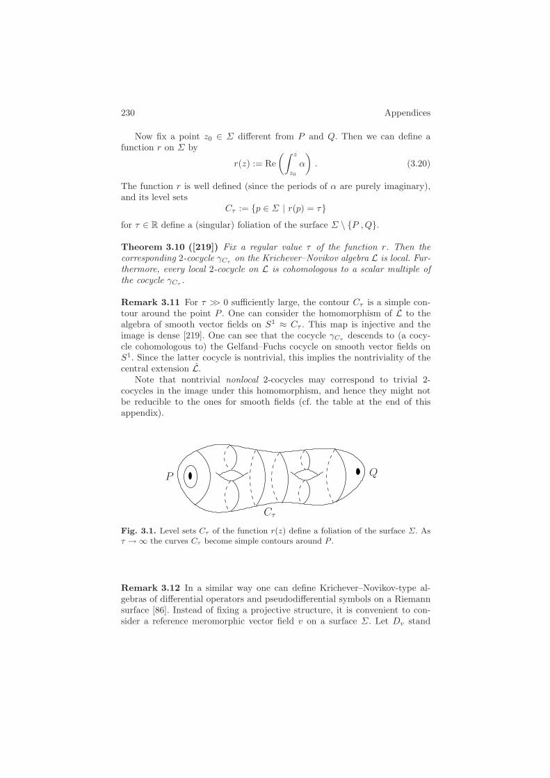
230 Appendices
Now fix a point z0 ∈ Σ different from P and Q. Then we can define afunction r on Σ by
r(z) := Re(∫ z
z0
α
)
. (3.20)
The function r is well defined (since the periods of α are purely imaginary),and its level sets
Cτ := p ∈ Σ | r(p) = τfor τ ∈ R define a (singular) foliation of the surface Σ \ P ,Q.
Theorem 3.10 ([219]) Fix a regular value τ of the function r. Then thecorresponding 2-cocycle γCτ
on the Krichever–Novikov algebra L is local. Fur-thermore, every local 2-cocycle on L is cohomologous to a scalar multiple ofthe cocycle γCτ
.
Remark 3.11 For τ >> 0 sufficiently large, the contour Cτ is a simple con-tour around the point P . One can consider the homomorphism of L to thealgebra of smooth vector fields on S1 ≈ Cτ . This map is injective and theimage is dense [219]. One can see that the cocycle γCτ
descends to (a cocy-cle cohomologous to) the Gelfand–Fuchs cocycle on smooth vector fields onS1. Since the latter cocycle is nontrivial, this implies the nontriviality of thecentral extension L.
Note that nontrivial nonlocal 2-cocycles may correspond to trivial 2-cocycles in the image under this homomorphism, and hence they might notbe reducible to the ones for smooth fields (cf. the table at the end of thisappendix).
QP
Cτ
Fig. 3.1. Level sets Cτ of the function r(z) define a foliation of the surface Σ. Asτ → ∞ the curves Cτ become simple contours around P .
Remark 3.12 In a similar way one can define Krichever–Novikov-type al-gebras of differential operators and pseudodifferential symbols on a Riemannsurface [86]. Instead of fixing a projective structure, it is convenient to con-sider a reference meromorphic vector field v on a surface Σ. Let Dv stand
A.3. Krichever–Novikov Algebras 231
for the Lie derivative along the field v. In a neighborhood of the point P weexpand meromorphic pseudodifferential symbols on Σ into a power series inDv, similar to the case of symbols on the circle; cf. Section II.4. The coefficientat D−1
v can be understood as a meromorphic 1-form on Σ, and let TrP be theresidue of this 1-form at the point P . Then there is a nontrivial 2-cocycle onmeromorphic pseudodifferential symbols defined by
cP (A,B) = TrP ([logDv, A] B]) ,
similarly to the circle case. In particular, one recovers the 2-cocycle (3.19) ofthe Krichever–Novikov algebra L of meromorphic vector fields on Σ. Thesealgebras of meromorphic differential operators and pseudodifferential symbolsalso have an analogue of the almost grading property of L.
3.4 Affine Krichever–Novikov Algebras, Coadjoint Orbits, andHolomorphic Bundles
To describe the affine algebras of Krichever–Novikov-type we fix a compactRiemann surface Σ with two marked points P, Q ∈ Σ. Let F denote theassociative algebra of meromorphic functions on Σ that can have poles only atthe points P and Q. Furthermore, fix a finite-dimensional complex semisimpleLie algebra g. The Krichever–Novikov current algebra is defined as the Liealgebra of g-valued meromorphic functions on Σ:
KN := g ⊗F .
One can show that the Lie algebra KN admits an almost grading and thereexists a unique local 2-cocycle on the Lie algebra KN given by
γaffCτ
(X,Y ) =1
2πi
∫
Cτ
tr(XdY ) ,
where the contour Cτ is a level set of the function r defined by formula (3.20).The affine Krichever–Novikov algebra KN is the central extension of the cur-rent algebra KN defined by means of the 2-cocycle γaff
Cτ. As a vector space it
is given byKN = g ⊗F ⊕ C .
Denote by Ω the space of meromorphic 1-forms on the surface Σ that canhave poles only at the points P and Q. The pairing F ×Ω → C between thefunctions and the forms is given by
〈f, ω〉 =1
2πi
∫
Cτ
fω ,
where f ∈ F and ω ∈ Ω. It turns out to be well defined (i.e., independent of τ)and nondegenerate. This allows one to view the space g ⊗Ω ⊕ C of g-valued
232 Appendices
1-forms on Σ enlarged by a cocentral direction as a “regular part” KN∗reg of
the dual of the affine Krichever–Novikov algebra KN = g ⊗ F ⊕ C. Here thepairing between KN and KN
∗reg = g ⊗Ω ⊕ C is given by the natural pairing
〈(X, c), (A, a)〉 =1
2πi
∫
Cτ
tr(XA) + c · a ,
for X ∈ g ⊗F and A ∈ g ⊗Ω.Let G denote the complex finite-dimensional simply connected Lie group
corresponding to the Lie algebra g. We denote by GΣ\P,Q the group of mapsfrom the Riemann surface Σ to G that are holomorphic outside the pointsP and Q. The group GΣ\P,Q transforms elements of the space KN
∗reg =
g ⊗Ω ⊕ C by means of the gauge transformations
g : (A, a) → (gAg−1 + a(dg)g−1, a) .
However, the space g⊗Ω⊕C is not invariant under this action. Define an orbitof the group GΣ\P,Q in the space KN
∗reg = g⊗Ω⊕C to be the intersection
of a “true” orbit of GΣ\P,Q with the space KN∗reg; see [353]. Equivalently,
one could consider the subgroup of GΣ\P,Q that leaves the space KN∗reg
invariant. In any case, these orbits are the analogues of the coadjoint orbits ofthe centrally extended loop groups that we studied in Section II.1.2. Let [Cτ ]denote the homotopy class of the level curve Cτ ⊂ Σ \ P,Q for τ >> 0.
Theorem 3.13 ([353, 354]) Generic orbits of the group GΣ\P,Q inside afixed affine hyperplane a = const = 0 in KN
∗reg are in one-to-one correspon-
dence with equivalence classes of representations ψ : π1(Σ \ P,Q) → G ofthe fundamental group of the punctured surface Σ \ P,Q such that ψ([Cτ ])is a semisimple (i.e., diagonalizable) element of the group G.
For the proof in one direction, one associates to an element (A, a) ∈ g⊗Ω⊕C
the monodromy group of the connection A meromorphic on the Riemann sur-face Σ and holomorphic on Σ \ P,Q. In the other direction, one has tocheck that any monodromy representation indeed comes from such a connec-tion. This is where the assumption on the semisimplicity of ψ([Cτ ]) comesinto play.
Theorem 3.13 links the theory of affine Krichever–Novikov algebras tothe theory of holomorphic G-bundles (or moduli of flat connections) on theRiemann surface Σ, where a similar correspondence of symplectic leaves andmonodromy groups arises; see [354] and the references therein for more detail.
Remark 3.14 To visualize the role of the Krichever–Novikov-type algebrasamong other algebras discussed in the book, we will allow nonlocal 2-cocycles.They can be defined as cocycles γC associated to arbitrary contours C on theRiemann surface Σ, not necessarily from the Cτ family. Independent cycles
A.3. Krichever–Novikov Algebras 233
in H1(Σ \ P,Q) lead to independent 2-cocycles γC . Note that all cycles Cτ
define a one-dimensional subspace in the homology group H1(Σ \ P,Q).While the affine/Virasoro algebras on C
∗ are graded versions of the corre-sponding smooth affine/Virasoro algebras on S1, the Krichever–Novikov typealgebras provide an almost graded version of affine and Virasoro algebras onarbitrary graphs on Riemann surfaces. Different cycles in the graphs definenon-cohomologous 2-cocycles of the corresponding current algebras on thosegraphs, similar to different 2-cocycles γC .
In this way, both the affine/Virasoro and the Krichever–Novikov-type al-gebras are Lie algebras of currents or vector fields on one-dimensional objects(either in the smooth or in the (almost) graded versions). These objects cor-respond to the R-part in our complexification table (see Section III.4), sincethese currents depend on one variable (either real or complex). Meanwhile,the C-part of the table corresponds to the Etingof–Frenkel-type algebras onan elliptic curve or on complex curves of higher genus. Here an elliptic curve isa complexification of a circle, while arbitrary complex curves of higher genuscan be regarded as complexifications of graphs. In the Etingof–Frenkel alge-bras their elements, i.e., currents, depend on two independent variables. Thisdiscussion is summarized in the following table:
“Real” (almost) Real smooth Complex smoothgraded version version version
Graded affine algebras Smooth affine Etingof–Frenkel algebrason C
∗ = CP1 \ P,Q algebras on S1 on elliptic curves E
Krichever–Novikov current Smooth affine Etingof–Frenkelalgebras on Riemann algebras algebras
surfaces Σ \ P1, . . . , Pn on graphs Γ on complex curves C
The affine algebras on graphs and their relation to the Etingof–Frenkelalgebras on curves of higher genus seem to be very interesting objects ofstudy, where still most of the work is yet to be done.
For more facts on Krichever–Novikov algebras and the proofs of the theo-rems in this section we refer to the original papers by Krichever and Novikov[219, 220], the works [336, 337, 353, 354, 379], and the references therein.
234 Appendices
A.4 Kahler Structures on the Virasoro and Loop GroupCoadjoint Orbits
4.1 The Kahler Geometry of the Homogeneous Space Diff(S1)/S1
Symplectic Structures
Consider the group Diff(S1) of orientation-preserving diffeomorphisms of thecircle S1, and identify S1 with the subgroup of rigid rotations Rot(S1). Inthis section we study geometric structures on the quotient
S = Diff(S1)/S1
that are invariant under the natural (left) action of the group Diff(S1) on S.The invariant structures are determined by their values at the point e ∈ S.
The tangent space at this point can be identified with the space of vector fieldson S1 with zero mean:
TeS ∼= Vect0(S1) =
ξ(θ)∂θ ∈ Vect(S1)∣
∣
∣
∫
S1ξ(θ) dθ = 0
.
(As usual, we denote a coordinate on S1 by θ and ∂θ stands for ∂∂θ .) Regard
the vector field ξ as an element of the complexified tangent space TeS ⊗ C
and expand ξ into the Fourier series
ξ =∑
n=0
ξnLn ,
where Lnn∈Z denotes the standard basis of VectC(S1), i.e., Ln = ieinθ∂θ.The real Lie algebra Vect(S1) ⊂ VectC(S1) is singled out by the relations−ξn = ξ−n.
Any invariant symplectic structure on the space S is also determined byits values at e ∈ S. In particular, it is defined by a continuous 2-cocycle ω onthe Lie algebra VectC(S1) that is invariant under rotations. More generally,invariant closed 2-forms on coadjoint orbits of a Lie group are related to 2-cocycles on the corresponding Lie algebra in the following way.
Exercise 4.1 Let G be a Lie group with Lie algebra g, and O ⊂ g∗ is a groupcoadjoint orbit. Given a point a ∈ O of the orbit, show that G-invariant closed2-forms ω on the orbit O are in one-to-one correspondence with 2-cocycles onthe Lie algebra g that vanish on the stabilizer of the point a. (Hint: Identifythe tangent space TaO for a ∈ O with a quotient of g. Use this to lift theG-invariant 2-form ω on O to a bilinear form on g. The closedness of ω on Ois equivalent to the cocycle identity of this bilinear form on g.)
A.4. Kahler Structures 235
In the case of the algebra Vect(S1), the proof of Proposition II.2.3 showsthat any invariant 2-cocycle has the form
ωα,β(Lm, Ln) := (αm3 + βm)δm,−n
for some constants α, β ∈ R.
Exercise 4.2 Show that the 2-cocycle ωα,β is nondegenerate on Vect0(S1)provided that either α = 0 and β = 0, or −β/α = k2 for some k ∈ N.
As we have seen in the proof of Proposition II.2.3, the cocycle ω0,β is exact,i.e., it is a coboundary. So to describe nontrivial 2-cocycles we can assume thatα = 0, and that −β/α is not an integer square.
The two-parameter family of symplectic structures on the space S definedby the 2-forms ωα,β has a natural interpretation in terms of coadjoint orbits ofthe Virasoro–Bott group. Indeed, the Virasoro–Bott coadjoint orbit containingthe point (p(dθ)2, a) ∈ vir
∗ is isomorphic to Diff(S1)/S1 if 0 < 4p/a is not aninteger square; see Section II.2.2. (If 4p/a = n2 for some n ∈ Z, the stabilizer ofthe point (p(dθ)2, a) is a three-dimensional subgroup of Diff(S1).) One can seethat the two-parameter family of symplectic structures on the space S comesfrom the identification of S with any coadjoint orbit from the two-parameterfamily of those in the Virasoro–Bott group. The natural symplectic structureof the coadjoint orbit through the point (p(dθ)2, a) ∈ vir
∗ with a = 0 and0 < 4p/a = n2 has two parameters: p and a.
The Complex Structure
A Diff(S1)-invariant almost complex structure on the space S = Diff(S1)/S1
is given by an S1-invariant automorphism Ie of the tangent space TeS ∼=Vect0(S1) such that I2
e = − id. Such an automorphism can be described usingthe Fourier expansion of an element ξ ∈ Vect0(S1): for
ξ =∑
n=0
ξnLn
we setIe(ξ) = −i
∑
n>0
ξnLn + i∑
n<0
ξnLn .
Exercise 4.3 Show that the almost complex structure I on the space S iscompatible with the symplectic structure ωα,β in the sense that ωα,β is I-invariant, i.e., ωα,β(Ieξ, Ieη) = ωα,β(ξ, η) at e ∈ S, and the symmetric bilinearform gα,β defined on the tangent space TeS by gα,β(ξ, η) := ωα,β(ξ, Ieη) ispositive definite.

236 Appendices
One can easily see that the almost complex structure I on the space S is“formally integrable”: the bracket of two vector fields in the +i, respectively−i, eigenspace of the automorphism I is again in the +i, respectively −i,eigenspace [57]. In principle, this does not guarantee the existence of a complexstructure in the infinite-dimensional context, since here the finite-dimensionalNewlander–Nirenberg theorem does not work. The following theorem of Kir-illov shows that the complex structure does exist in this infinite-dimensionalcase.
Theorem 4.4 ([204]) There is a complex structure on the space S =Diff(S1)/S1 invariant with respect to the Diff(S1)-action.
Sketch of proof. To show that the almost complex structure on S is, infact, integrable, one can give a different realization of the space S in termsof univalent functions on the unit disk. Namely, let D ⊂ C be the unit disk,and set F to be the space of holomorphic univalent functions on D that arecontinuous up to the boundary and normalized by the conditions at the origin:
F = f : D →C | f holomorphic and continuous up to the boundary,f(0) = 0, f ′(0) = 1, and f(z1) = f(z2) whenever z1 = z2 .
This is an infinite-dimensional complex manifold. By expanding f in a series
f(z) = z + c2z2 + c3z
3 + · · ·
one obtains a natural coordinate system on the space F . De Brange’s theorem(formerly the Bieberbach conjecture, [212]) implies that |ck| < k, so that Fcan be regarded as an infinite-dimensional analogue of a bounded domain inC
n, see [204].The identification of F with the quotient S = Diff(S1)/S1 is implemented
by means of the following geometric realization. Identify F with the spaceK of all simple contours around the origin that have conformal radius 1 withrespect to the origin. Namely, a univalent function f ∈ F uniquely determinessuch a contour as the image f(S1) of the boundary S1 = ∂D. Conversely, forany such contour K ∈ K there is a function fK mapping its interior to theunit disk (the Riemann mapping theorem), which can be normalized so thatfK ∈ F .
To see how one can associate a coset from Diff(S1)/S1 to a function fK ,consider a function gK mapping the exterior of the unit disk D to the exteriorof the contour K and normalized by the condition gK(∞) = ∞. This functionis defined modulo the rotation change of the variable z → eiαz. Then the mapφK = f−1
K gK defines a diffeomorphism of the unit circle S1 = ∂D modulorotations, i.e., an element of S = Diff(S1)/S1.
This map is a bijection, and the definition of the inverse map from S to F isas follows. Given a circle diffeomorphism φ ∈ Diff(S1) construct a 2-sphere S2
φ

A.4. Kahler Structures 237
by glueing together the boundaries of the two unit disks D− and D+ accord-ing to that diffeomorphism. There is a unique complex structure on S2
φ thatcoincides with the standard ones on D− and D+. Since all complex structureson S2 are equivalent, there exists a holomorphic map F : S2
φ → S2 = CP1
that can be normalized by the conditions F (0) = 0, F ′(0) = 1, F (∞) = ∞. Inturn, the map F can be thought of as a pair of functions F = (f, g) definedon D− and D+ (here 0 ∈ D− and ∞ ∈ D+), and one can see that f ∈ F . Thecorresponding contour K ∈ K is the image of the unit circle f(S1).
The group Diff(S1) acts on the space of contours and hence on the space Fby holomorphic transformations, and the stabilizer of the function f(z) = zunder this action is given by the group of rigid rotations S1 = Rot(S1) ⊂Diff(S1). This identification F ∼= S ∼= K fixes the complex structure on thespace S invariant with respect to the Diff(S1)-action.
The following theorem details and summarizes this section.
Theorem 4.5 ([204, 208]) The space S = Diff(S1)/S1 is a Kahler Frechetmanifold with a two-parameter family of Diff(S1)-invariant Kahler metricsgα,β. These Kahler metrics originate from one invariant complex structureand a two-parameter family of invariant symplectic structures on S.
Note that the Virasoro group can be viewed as a holomorphic C∗-bundle
over S [236].
4.2 The Action of Diff(S1) and Kahler Geometry on the BasedLoop Spaces
Symplectic Structures
Let G be a simple compact simply connected Lie group with the Lie algebrag. The loop group of G is the group LG = C∞(S1, G) of smooth maps fromthe circle S1 to G. The based loop group ΩG is the subgroup
ΩG = g ∈ LG | g(0) = e
for a fixed point 0 ∈ S1. As a manifold, ΩG can be identified with the quotientLG/G, where G is thought of as the subgroup in LG consisting of constantloops in G. Note, however, that this identification is not canonical, since G isnot a normal subgroup in LG.
An LG-invariant closed 2-form on the space ΩG is determined by its valueson the tangent space TeΩG ∼= Lg/g or, equivalently, by a G-invariant 2-cocycleω on the Lie algebra Lg that also satisfies g ⊂ kerω. Proposition II.1.6 showsthat any continuous G-invariant 2-cocycle on Lg has the form
ω(X,Y ) =∫
S1〈X(θ), Y ′(θ)〉 dθ ,
238 Appendices
where 〈 , 〉 is an invariant inner product on the Lie algebra g. Also, ω satisfiesthe condition g ⊂ kerω, since it vanishes on constant loops. The fact that the2-form ω is nondegenerate, i.e., it defines a symplectic structure on ΩG, isequivalent to the nondegeneracy of the inner product 〈 , 〉.
For a simple Lie group G there is the Killing form, the unique (up to ascalar factor) invariant inner product on g. Hence, in this case there existsa one-parameter family of LG-invariant symplectic forms on the space ΩG.This family appears naturally from the identification of the quotient LG/Gwith the coadjoint orbits of the affine (i.e., centrally extended loop) groupLG that contain the points (0, a) ∈ (Lg)∗: the parameter in this family is thecocentral value a = 0; see Section II.1.2.
Exercise 4.6 The group Diff(S1) acts on the space LG/G by symplecto-morphisms. (Hint: the cocycle ω, and hence the corresponding symplecticstructure, is invariant with respect to reparametrizations of S1.)
Complex Structures
Any LG-invariant almost complex structure on the based loop group ΩGis given by fixing an automorphism Je of the tangent space TeΩG such that(Je)2 = −1. In the complexification TC
e ΩG consider the set of Laurent polyno-mials (without the constant term) with values in the complexified Lie algebragC:
X(z) =∑
n=0
Xnzn .
Now we define an LG-invariant almost complex structure J0 on ΩG by as-signing its value on such polynomials to be
J0eX(z) = −i
∑
n>0
Xnzn + i
∑
n<0
Xnzn
and extending it to an automorphism of TeΩG by continuity.One can see that this almost complex structure is integrable by identifying
the based loop group ΩG with the quotient LGC/L+GC. Here, LGC denotesthe group of smooth maps from the circle S1 to the complexified Lie group GC,and L+GC denotes the subgroup of those maps that extend to holomorphicmaps from the unit diskD, the interior of the circle, to the groupGC. To obtainthis identification one employs the fact that any loop h ∈ LGC can be uniquelyfactorized into a product h = hb · h+ with hb ∈ ΩG and h+ ∈ L+GC; see[322]. Therefore the quotient LGC/L+GC carries an LGC-invariant complexstructure that coincides with J0
e at the identity.A diffeomorphism ϕ ∈ Diff(S1) sends the complex structure J0 to J =
ϕ∗ J0 ϕ−1∗ , where ϕ∗ denotes the action of the diffeomorphism ϕ on the
corresponding tangent space.
A.4. Kahler Structures 239
Proposition 4.7 The complex structure J = ϕ∗ J0 ϕ−1∗ coincides with J0
if and only if the diffeomorphism ϕ ∈ Diff(S1) is a rotation.
Sketch of proof. Evidently, if ϕ is a rotation, then J = J0. Conversely,assume that J = J0. Recall that the complex structure J0 on ΩG is defined bymeans of the identification of the latter with the quotient ΩG = LGC/L+GC.Then the action of the diffeomorphism ϕ preserves the representation of ΩG =LGC/L+GC as a quotient, i.e., it sends the subgroup L+GC into itself.
Denote by L−1 G
C the subset of LGC consisting of loops in GC that extendto holomorphic maps h from the exterior of the unit disk to GC and thatare normalized by the condition h(∞) = id ∈ GC. The multiplication mapL−
1 GC×L+GC → LGC is a diffeomorphism to a dense subset of LGC; see [322,
Section 8.6] One can show that in order to preserve the complex structure onΩG, the diffeomorphism ϕ has to preserve both L−
1 GC and L+GC. This implies
that the circle diffeomorphism ϕ extends to both a conformal automorphism ofthe unit disk D and to a conformal automorphism of the exterior of the disk Dfixing ∞; cf. the proof of Theorem 4.4 above. Such a conformal automorphismof the Riemann sphere has to be a rotation, and so is ϕ itself.
The complex structures J = ϕ∗ J0 ϕ−1∗ obtained from the complex
structure J0 by the action of the diffeomorphism group Diff(S1) are calledadmissible complex structures on ΩG. By construction of J0, all admissiblecomplex structures are LG-invariant. From the proposition above, we directlyobtain the following result:
Corollary 4.8 ([57, 312]) Admissible complex structures on the based loopgroup ΩG are parametrized by the points of the infinite-dimensional manifoldS = Diff(S1)/S1.
Finally, one can verify that the complex structure J0 is compatible withthe symplectic structure ω in the sense that ω(J0X,J0Y ) = ω(X,Y ), whileg0(X,Y ) := ω(X,J0Y ) is a positive definite quadratic form. Hence, g0 definesan LG-invariant Kahler metric on ΩG. In view of the invariance of the sym-plectic form ω under the action of the group Diff(S1), the complex structuresJ = ϕ∗ J0 ϕ−1
∗ obtained from J0 are also compatible with the symplecticform ω and thus give rise to a family of LG-invariant Kahler metrics g on ΩGparametrized by the points of S = Diff+(S1)/S1.
This description of Kahler metrics exhibits a kind of reciprocity betweenthe homogeneous spaces LG/G and Diff+(S1)/S1. More details, the formulasfor the corresponding curvature tensor, and further applications of the abovecan be found in [204, 208, 350].

240 Appendices
A.5 Diffeomorphism Groups and Optimal MassTransport
In this appendix we consider the Riemannian geometry of the group of alldiffeomorphisms of a compact manifold. This large group, being equipped witha certain L2-type metric, can be viewed as a unifying framework for problemsof Euler hydrodynamics on the group of volume-preserving diffeomorphismson the one hand and problems related to optimal mass transportation ondensities on this manifold on the other hand.
5.1 The Inviscid Burgers Equation as a Geodesic Equationon the Diffeomorphism Group
Let M be a compact n-dimensional Riemannian manifold with metric ( , ).Consider the group Diff(M) of smooth diffeomorphisms of M along with itssubgroup SDiff(M) of diffeomorphisms preserving the (Riemannian) volumeform µ (as before, we confine ourselves to the connected component of theidentity diffeomorphism). For a curve η(t) | t ∈ [0, a] in Diff(M) its L2-energy is given by
E(η) =12
∫ a
0
〈η(t), η(t)〉Diff dt ,
where the (weak) Riemannian metric at each point η ∈ Diff(M) of the dif-feomorphism group is defined in the following straightforward way: givenX,Y ∈ Vect(M), the inner product of two vectors X η, Y η ∈ TηDiff(M) is
〈X η, Y η〉Diff =∫
M
(X η(x), Y η(x)) µ(x). (5.21)
This metric is right-invariant when restricted to the subgroup SDiff(M) ofvolume-preserving diffeomorphisms, although it is not right-invariant on thewhole group Diff(M). (Indeed, the change of variables in the integral (5.21)would give the Jacobian det[∂η/∂x] as an extra factor, which, however, isidentically equal to 1 for a volume-preserving map η ∈ SDiff(M).) Note thatfor a flat manifold M this metric is a flat metric on Diff(M): a neighborhoodof the identity id ∈ Diff(M) with the metric 〈 , 〉Diff is isometric to a neigh-borhood in the pre-Hilbert space of smooth “vector-functions” η : M → Mwith the L2 inner product 〈 , 〉L2(M).
Recall that the Euler equation ∂tu+ (u,∇)u = −∇p on a divergence-freefield u on M describes the motion of an ideal incompressible fluid filling M .It corresponds to the equation of the geodesic flow of the right-invariant L2
metric on the group SDiff(M); see [12] and Section II.3.Define the (inviscid) Burgers equation as the evolution equation
∂tu+ (u,∇)u = 0 (5.22)
A.5. Diffeomorphism Groups and Optimal Mass Transport 241
for a vector field u on M , where (u,∇)u stands for the covariant derivative∇uu on M . (This equation is often also called the Hopf equation or compress-ible Euler equation.) Consider the flow (t, x) → η(t, x) corresponding to thisvelocity field:
∂tη(t, x) = u(t, η(t, x)), η(0, x) = x.
(Here we use the notation ∂tη(t, x) for the time derivative η to emphasize thedependence of η on both t and x.)
Proposition 5.1 ([96, 303]) (1) Solutions of the Burgers equation are time-dependent vector fields on M that describe the following flows of fluid particles:each particle moves with constant velocity (defined by the initial condition)along a geodesic in M .
(2) Geodesics in the group Diff(M) with respect to the L2-metric (5.21)correspond to solutions of the Burgers equation. Geodesics in Diff(M) normalto the submanifold SDiff(M) have potential initial conditions.
Proof. We first assume for simplicity that M is equipped with a flat metric.Then the geodesics in Diff(M) are given by the equation η(t) = 0, whichdescribes flows of particles moving with constant velocity along their owngeodesics, “straight lines,” in M . This follows from the “flatness” of the L2-metric (5.21). Indeed, consider a one-parameter variation ηs(t) of a curveη(t) with fixed ends for all s. Let w(t) := ∂sηs(t)|s=0 be the variationvector field along the curve η(t), and w(0) = w(a) = 0. Then the geodesiccondition on η(t), i.e., vanishing of the variation ∂sE(ηs) = 0 at s = 0, gives
0 =∫ a
0
〈∂sηs(t), ηs(t)〉L2(M) dt∣
∣
∣
s=0
=∫ a
0
〈w(t), η(t)〉L2(M) dt = −∫ a
0
〈w(t), η(t)〉L2(M) dt .
This implies η(t) = 0 and proves (1) in the flat case.In order to see that the corresponding velocity field u for the geodesic
η(t) | ∂2t η = 0 satisfies the Burgers equation, we apply the chain rule to the
definition ∂tη(t, x) = u(t, η(t, x)). This immediately gives
∂2t η = ∂tu(t, η(t, x)) = (∂tu+∂xu ·∂tη)(t, η(t, x)) =
(
∂tu+(u,∇)u)
(t, η(t, x)),
and hence the geodesic condition d2η/dt2(t, x) = 0 is equivalent to the Burgersequation on M :
∂tu+ (u,∇)u = 0 .
(One can compare the latter to the Euler equation on the subgroupSDiff(M) ⊂ Diff(M), where the acceleration ∂2
t η is L2-orthogonal to the setSDiff(M) and hence is given by a gradient field, cf. Section II.3.2.)
In the general case, any Riemannian metric on M induces a unique Levi-Civita L2-connection ∇ on Diff(M), which is determined pointwise by the
242 Appendices
Riemannian connection ∇ on the manifold M itself (see for example [96] or[267]). Then the same chain rule leads to the Burgers equation (5.22) onvelocity u with (u,∇)u := ∇uu. The latter is equivalent to the Riemannianversion of freely flying non-interacting particles in M : ∇η η = 0. The flowcorresponding to the Burgers solution with the initial field v(x) on M has theform x → expM (t · v(x)), where expM stands for the Riemannian exponentialmap on the manifold M . This is a family of diffeomorphisms (parametrized bytime t) in which each point moves along its own geodesic on M with constantvelocity.
Finally, observe that the tangent space to the subgroup SDiff(M) at theidentity consists of divergence-free vector fields, and hence the space of nor-mals is given by the gradients of all smooth functions on M . Thus horizontalgeodesics are the ones whose initial velocities are gradient fields u|t=0 = ∇φ;see Figure 5.1.
Remark 5.2 For a smooth initial velocity field u|t=0 = v, the family x →exp(t · v(x)) consists of diffeomorphisms for small t, but at some momentparticles can start colliding with each other. This moment corresponds toformation of a shock wave on M , and from this moment on, the map frominitial to final positions of the particles ceases to be a diffeomorphism. Inother words, the group Diff(M) is incomplete in the L2-metric (5.21) and thecorresponding geodesics “reach the boundary of the group” Diff(M) in finitetime.
One can show that the shock wave formation for the Burgers equationwith potential initial condition u|t=0 = ∇φ corresponds to the first focalpoint in the direction ∇φ, which is normal to the set SDiff(M) regarded as aRiemannian submanifold of Diff(M); see [193] and Figure 5.1. Recall that afocal point of a submanifold S in a Riemannian manifold N in the directionν normal to S is the point of intersection of normals to S that are infinitelyclose to ν.
Example 5.3 The Burgers equation on the line assumes the form ∂tu+uu′ =0, where u′ := ∂xu. Faster particles start passing slower ones, and one cansee that the shock wave solutions of the Burgers equation first arise frominflection points of the initial velocity profile of u|t=0 (i.e., from the pointscorresponding to u′′|t=0 = 0).
In higher dimensions the shock waves first arise from the special points ofthe initial potential u|t=0 = ∇φ, which are singularities of type A3 modulocertain linear and quadratic terms in local orthogonal coordinate charts; see[46]. The list of initial singularities, possible bifurcations of the shock waves,and other related questions for the inviscid Burgers equations can be foundin [21, 22, 137].
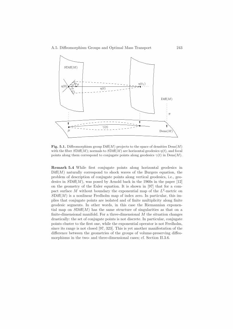
A.5. Diffeomorphism Groups and Optimal Mass Transport 243
η(0)
SDiff(M)
γ(t)¹
∇φ η(t1)
Dens(M)
¼
η(t)
Diff(M)
Fig. 5.1. Diffeomorphism group Diff(M) projects to the space of densities Dens(M)with the fiber SDiff(M); normals to SDiff(M) are horizontal geodesics η(t), and focalpoints along them correspond to conjugate points along geodesics γ(t) in Dens(M).
Remark 5.4 While first conjugate points along horizontal geodesics inDiff(M) naturally correspond to shock waves of the Burgers equation, theproblem of description of conjugate points along vertical geodesics, i.e., geo-desics in SDiff(M), was posed by Arnold back in the 1960s in the paper [12]on the geometry of the Euler equation. It is shown in [97] that for a com-pact surface M without boundary the exponential map of the L2-metric onSDiff(M) is a nonlinear Fredholm map of index zero. In particular, this im-plies that conjugate points are isolated and of finite multiplicity along finitegeodesic segments. In other words, in this case the Riemannian exponen-tial map on SDiff(M) has the same structure of singularities as that on afinite-dimensional manifold. For a three-dimensional M the situation changesdrastically: the set of conjugate points is not discrete. In particular, conjugatepoints cluster to the first one, while the exponential operator is not Fredholm,since its range is not closed [97, 323]. This is yet another manifestation of thedifference between the geometries of the groups of volume-preserving diffeo-morphisms in the two- and three-dimensional cases; cf. Section II.3.6.
244 Appendices
5.2 Metric on the Space of Densities and the Otto Calculus
The differential geometry of diffeomorphism groups is closely related to thetheory of optimal mass transport, and in particular, to the problem of movingone mass (or density) to another while minimizing a certain cost. In thissection we discuss the relation of metric properties of the diffeomorphismgroup and the space of densities.
Let µ be a smooth reference volume form (or density) on M of unit totalmass, and consider the projection π : Diff(M) → Dens(M) of diffeomorphismsonto the space Dens(M) of (normalized) smooth densities on M . The diffeo-morphism group Diff(M) is fibered over Dens(M) by means of this projectionπ as follows: the fiber over a volume form ν consists of all diffeomorphismsη that push µ to ν, η∗µ = ν. In other words, two diffeomorphisms η1 and η2
belong to the same fiber if and only if η1 = η2 ϕ for some diffeomorphism ϕpreserving the volume form µ. Diffeomorphisms from Diff(M) act transitivelyon smooth densities, according to the Moser theorem [279].
Remark 5.5 Note that this projection π can be extended to more general(nonsmooth) maps and densities by tracing how they transport the densityµ. More precisely, let µ and ν be two Borel measures of total volume 1 on acompact Riemannian manifold M (or, more generally, on a complete metricspace) that are absolutely continuous with respect to the Lebesgue measure,and let dist(x, y) be the distance function on M . Consider the following opti-mal mass transport problem: Find a Borel map η : M → M that pushes themeasure µ forward to ν and attains the minimum of the L2-cost functional∫
Mdist2(x, η(x))µ among all such maps. The minimal cost of transport de-
fines a metric (often called the Kantorovich or Wasserstein metric) Dist ondensities:
Dist2(µ, ν) := infη
∫
M
dist2(x, η(x))µ | η∗µ = ν
. (5.23)
It turns out that this mass transport problem admits a unique solution(defined up to measure-zero sets), called the optimal map η (see [58] for M =R
n and [256] for any compact connected Riemannian manifold M withoutboundary). Furthermore, there exists a 1-parameter family of Borel maps η(t)joining the identity map η(0) = id with the optimal map η(1) = η such thatη(t) pushes µ to η(t)∗µ in an optimal way for every t. Such a 1-parameterfamily of measures η(t)∗µ describes a geodesic between µ and ν in the spaceof densities with respect to the metric Dist; see [374] for details.
In what follows we consider a formal version of this problem, focusing onsmooth densities. One can see that the Kantorovich metric Dist is formallygenerated by the (weak) Riemannian metric on the space Dens of smoothdensities. Thus both Diff and Dens can be regarded as infinite-dimensionalRiemannian manifolds.

A.5. Diffeomorphism Groups and Optimal Mass Transport 245
Proposition 5.6 ([303]) The bundle map π : Diff(M) → Dens(M) is aRiemannian submersion of the metric 〈 , 〉Diff on the diffeomorphism groupDiff(M) to the metric Dist on the density space Dens(M). The horizontal(i.e., normal to fibers) spaces in the bundle Diff(M) → Dens(M) are right-translated gradient fields.
Recall that for two Riemannian manifolds P and B a submersion π :P → B is a mapping onto B that has maximal rank and preserves lengthsof horizontal tangent vectors to P ; see, e.g., [302]. For a bundle P → B thismeans that on P there is a distribution of horizontal spaces that are orthogonalto fibers and projected isometrically to the tangent spaces to B.
Proof. Recall the Hodge decomposition Vect = SVect ⊕L2 Grad for vectorfields on M : any vector field v decomposes uniquely into the sum v = ξ +∇pof a divergence-free field ξ and a gradient field ∇p, which are L2-orthogonalto each other:
∫
M(ξ,∇p)µ = 0; cf. Section II.3.16
For the fibration π : Diff(M) → Dens(M) the fiber passing through theidentity diffeomorphism id ∈ Diff(M) is the subgroup SDiff(M), preservingthe reference density µ itself. Thus the vertical tangent space at the identitycoincides with SVect(M), while the horizontal space is Grad. The L2-metricon Grad projects isometrically to the tangent space to the base Dens at thepoint µ.
Other fibers of Diff(M) → Dens(M) are right cosets for the subgroupSDiff(M) in the group Diff(M). One can think of this fibration as anSDiff(M)-principal bundle over Dens(M), where volume-preserving diffeo-morphisms from SDiff(M) act on all diffeomorphisms by right translationsRϕ : η → η ϕ for ϕ ∈ SDiff(M) and η ∈ Diff(M). This induces the SDiff-action on the corresponding tangent spaces. The metric (5.21) is invariantwith respect to this action of SDiff(M).
Now the proposition follows from the Hodge decomposition above, whichis right-translated from id to any other point η of the diffeomorphism groupDiff(M). The vertical space (tangent to a fiber) at a point η ∈ Diff(M) consistsof divergence-free vector fields right-translated by the diffeomorphism η,
Vertη = X η | X ∈ SVect(M) ,
while the horizontal space is given by the translated gradient fields,
Horη = (∇p) η | p ∈ C∞(M,R).
The L2-type metric 〈 , 〉Diff on horizontal spaces for different points of thesame fiber projects isometrically to one and the same metric on the base, dueto the SDiff-invariance of the metric. 16 More generally, one can consider the volume form µ not related to the Riemannian
metric ( , ). The L2-orthogonality still holds for µ-divergence-free fields andgradients with respect to this metric.
246 Appendices
One of the main properties of a Riemannian submersion is the followingfeature of geodesics:
Corollary 5.7 Any geodesic initially tangent to a horizontal space on thefull diffeomorphism group Diff(M) remains horizontal, i.e., tangent to thegradient distribution Horη on this group. There is a one-to-one correspondencebetween geodesics on the base Dens(M) starting at the density µ and horizontalgeodesics in Diff(M) starting at the identity diffeomorphism id.
Remark 5.8 In PDE terms, the horizontality of a geodesic means that anysolution of the Burgers equation with a potential initial condition u = ∇φremains potential for all times. The corresponding potential φ satisfies theHamilton–Jacobi equation ∂tφ+ (∇φ,∇φ)/2 = 0 on M ; see [303].
Thus horizontal geodesics in Diff(M), i.e., potential solutions of the Burg-ers equation, move the densities in Dens(M) in the fastest way. This statementis very natural geometrically: to obtain the fastest projection to the base, i.e.,to move densities most effectively, one has to mod out the “volume-preserving”parts of the diffeomorphisms (since they are not moving the density, but pre-serve it), and use only their “gradient parts.”
Remark 5.9 Consider the flow η(t) : x → expM (t · ∇φ(x)) correspondingto the potential Burgers solution with a given smooth potential φ. As wementioned, the solution remains smooth for some time, and the appearanceof a shock wave corresponds to the first moment at which the solution isnonsmooth. For M = R
n the map x → expM (t · ∇φ(x)) has the form x →x + t · ∇φ(x) = ∇(x2/2 + t · φ(x)), and the loss of the map’s smoothnesscorresponds to the loss of convexity of the potential f(x) := x2/2 + t · φ(x).On any M this loss of smoothness occurs when the potential −t φ ceases tobe c-concave, which is an analogous notion for manifolds. (A function ψ on amanifold M is c-concave if (ψc)c = ψ, where ψc(y) := infc(x, y)−ψ(x) | x ∈M for the square distance function c(x, y) = dist2(x, y)/2 on M .) As longas the potential remains c-concave, the curve η(t) is the shortest curvein Diff(M) joining its endpoints, while its projection to Dens(M) gives theshortest curve joining the corresponding densities. This description is basedon the following theorem on polar decomposition: every diffeomorphism η ∈Diff(M) has a unique decomposition η = gr ϕ into a “gradient map” gr(x) :=expM (∇φ(x)) for a c-concave potential −φ and a volume-preserving map ϕof M ; see [61, 256].
We return to the problem of finding optimal maps for moving the densityµ(x) to any other density ν(y) = h(y)µ(y), where h is a function on M . TheJacobian of a map η that sends µ to ν = η∗µ satisfies the relation
h(η(x)) · det[∂η/∂x] = 1 .
A.5. Diffeomorphism Groups and Optimal Mass Transport 247
The polar decomposition theorem implies that in Rn the optimal map is the
gradient η = ∇f of a convex potential f , and the above relation assumes theform of the Monge–Ampere equation on the potential:
det(Hess f(x)) =1
h(∇f(x)),
where Hess f := ∂(∇f)/∂x is the Hessian matrix of the function f . For amanifold M the potential for the optimal map expM (∇φ) also satisfies theMonge–Ampere-like equation
det[∂ expM (∇φ)
∂x
]
=1
h(expM (∇φ(x))),
where expM is the Riemannian exponential on the manifold M and −φ is ac-concave potential. We refer to the books [374, 375] and papers [58, 256, 303]for a comprehensive discussion of optimal transport.
5.3 The Hamiltonian Framework of the Riemannian Submersion
The Riemannian submersion property for the fibration Diff(M) → Dens(M)can be put in the framework of symplectic reduction, discussed in Section I.5;see [235]. Recall the following general construction in symplectic geometry.Let π : P → B be a principal bundle with the structure group G.
Lemma 5.10 (see, e.g., [23]) The symplectic reduction of the cotangentbundle T ∗P over the G-action gives the cotangent bundle T ∗B = T ∗P//G.
Proof. The moment map Φ : T ∗P → g∗ associated with this action takesT ∗P to the dual of the Lie algebra g of the group G. For the G-action on T ∗Pthe moment map Φ is the projection of any cotangent space T ∗
aP to cotangentspace T ∗
aF ≈ g∗ for the fiber F through a point a ∈ P . The preimage Φ−1(0)of the zero value is the subbundle of T ∗P consisting of covectors vanishing onfibers. Such covectors are naturally identified with covectors on the base B.Thus factoring out the G-action, which moves the point a over the fiber F ,we obtain the bundle T ∗B.
Suppose now that P is equipped with a G-invariant Riemannian metric〈 , 〉P . Then it induces the metric 〈 , 〉B on the base B.
Lemma 5.11 The Riemannian submersion of P (P, 〈 , 〉P ) to the base B,equipped with the metrics 〈 , 〉P and 〈 , 〉B respectively, is the result of thesymplectic reduction with respect to the G-action.
248 Appendices
Proof. Indeed, the metric 〈 , 〉P gives a natural identification T ∗P ≈ TP ofthe tangent and cotangent bundles for P , and the “projected metric” is equiv-alent to a similar identification for the base manifold B. In the presence of themetric in P , the preimage Φ−1(0) is identified with the subbundle of horizontalspaces in TP : the zero value of the moment map stands for the orthogonal-ity to the vertical (i.e., tangent to the fibers) spaces. Hence the symplecticquotient Φ−1(0)/G can be identified with the tangent bundle TB.
Let HP : T ∗P → R be a Hamiltonian function invariant under the G-action on the cotangent bundle of the total space P . The restriction of thisfunction to the horizontal bundle (Φ−1(0) ⊂ T ∗P ) is also G-invariant, andhence descends to a function HB : T ∗B → R on the quotient, the cotan-gent bundle of the base B. One has the following reduction of Hamiltoniandynamics:
Proposition 5.12 ([23]) The Hamiltonian flow of the function HP pre-serves the preimage Φ−1(0); i.e., trajectories with horizontal initial conditionsstay horizontal. Furthermore, the Hamiltonian flow of the function HP on thecotangent bundle T ∗P of the total space descends to the Hamiltonian flow ofthe function HB on the cotangent bundle T ∗B of the base.
Apply the above consideration to our setting, in which P = Diff(M),G = SDiff(M), and B = Dens(M). The above lemmas give a Hamiltonianmeaning to Proposition 5.6 on Riemannian submersion.
Now we would like to describe the geodesics on the spaces Diff(M)and Dens(M). Recall that one of possible definitions of geodesics in anyRiemannian manifold M is that they are projections to M of trajectoriesof the Hamiltonian flow on T ∗M , whose Hamiltonian function is the “kineticenergy” KM (p, q) := (p, p)/2 given by this Riemannian metric. In the sameway, geodesics on Diff(M) and Dens(M) are obtained by considering the cor-responding Hamiltonians for the metric 〈 , 〉Diff and metric Dist, respectively.
It will be convenient for us to identify the tangent and cotangent spacesfor the manifold M , as well as those for the group Diff(M), using thecorresponding metrics on them. Consider also a more general Hamiltonianfunction HM on the (co)tangent bundle TM of the manifold M . The aver-aged Hamiltonian function is the function HDiff on the (co)tangent bundleTDiff(M) of the diffeomorphism group Diff(M) obtained by averaging thecorresponding Hamiltonian HM over M in the following way: its value at apoint X η ∈ TηDiff(M) is
HDiff(X η) :=∫
M
HM (X η(x))µ(x)
for a vector field X ∈ Vect(M) and a diffeomorphism η ∈ Diff(M). For in-stance, the energy Hamiltonian KDiff(Xη) := 1
2 〈Xη,Xη〉Diff on TDiff(M)is the averaging of the “kinetic energy” Hamiltonian KM defined on TM .

A.5. Diffeomorphism Groups and Optimal Mass Transport 249
Consider the Hamiltonian flows for the Hamiltonian functions HM andHDiff on the (co)tangent bundles TM and TDiff(M), respectively, relative tothe standard symplectic structures on the bundles.
Theorem 5.13 ([235]) Each Hamiltonian trajectory for the averaged Hamil-tonian functions HDiff on TDiff(M) describes such a flow on the tangentbundle TM in which every tangent vector to M moves along its own HM -Hamiltonian trajectory in TM .
This theorem has the following simple geometric meaning for the energyHamiltonians KDiff and KM . It implies that all geodesics on the diffeomor-phism group Diff(M) (described by the Burgers equation; see Proposition 5.1)starting at the identity id with the initial velocity X ∈ Vect(M) are the flowsthat move each particle x on the manifold M along the geodesic with theinitial direction X(x). Such a geodesic is well defined on the diffeomorphismgroup Diff(M) as long as the particles do not collide.
Furthermore, Proposition 5.12 implies that a geodesic on Diff(M) withpotential initial condition will stay potential (cf. Corollary 5.7). Finally, sincethe metric on Diff(M) is SDiff-invariant, so is the energy Hamiltonian KDiff,and hence it descends to the energy Hamiltonian on TDens(M). The latterdescribes the geodesics on the density space Dens(M) with respect to the met-ric Dist. This way one recovers the geodesic properties of the group Diff(M)discussed above.
Remark 5.14 For a more general Hamiltonian HM on the tangent bun-dle TM , each particle x ∈ M with an initial velocity X(x) will be movingalong its characteristic, which is the projection to M of the correspondingHamiltonian trajectory in the tangent bundle TM . This description for moregeneral Hamiltonians allows one to extend the above description of geodesicsto other situations, and in particular, to the case of nonholonomic distributions(i.e., to sub-Riemannian, or Carnot–Caratheodory, spaces); see [9, 188, 235].
Note that the above Hamiltonian framework is also valid for more generalcost functions c : M ×M → R, which can replace dist2 in the mass transportproblem (5.23).

250 Appendices
A.6 Metrics and Diameters of the Group of HamiltonianDiffeomorphisms
6.1 The Hofer Metric and Bi-invariant Pseudometricson the Group of Hamiltonian Diffeomorphisms
Let M be a symplectic manifold of dimension 2n with a symplectic form ω.Consider the space F(M) of Hamiltonian functions on M normalized in thefollowing way. For a closed manifold M we define F(M) as the space of smoothfunctions with zero mean with respect to the canonical volume form ωn. Foran open M , the space F(M) consists of all smooth functions with compactsupport. In either case, F(M) is a Lie algebra with respect to the Poissonbracket related to ω or, equivalently, the Lie algebra of the correspondingHamiltonian vector fields on M . (Note that this algebra can be endowed withan invariant inner product 〈H,K〉 :=
∫
MHK ωn, where H,K ∈ F(M).)
Consider the corresponding group Hamc(M) of all compactly supportedHamiltonian diffeomorphisms of M , which are time-one maps of time-dependent Hamiltonian fields with Hamiltonian functions from F(M). InSections II.3.6 and II.6.2 we saw that the infinite-dimensional group Ham(M),as well as Hamc(M), admits left-invariant lp-metrics, which depend on thechoice of a Riemannian metric on the manifold M . It turns out that thegroup Hamc(M) does in fact admit a bi-invariant metric, which depends onlyon the symplectic structure on M .
Definition 6.1 Set the energy of a Hamiltonian diffeomorphism ϕ ∈Hamc(M) to be
E(ϕ) := infH
(
supx,t
H(x, t) − infx,t
H(x, t))
,
where (x, t) ∈ M × [0, 1] and H runs over the set of all compactly supportedtime-dependent Hamiltonian functions H : M× [0, 1] → R whose Hamiltonianvector field has the given diffeomorphism ϕ as the time-one map. The Hofermetric defines the distance on the group Hamc(M) as
ρE(ψ,ϕ) = E(ψϕ−1)
for any two compactly supported Hamiltonian diffeomorphisms ψ and ϕ.
Exercise 6.2 Verify that
E(ϕ) = E(ϕ−1) = E(ψϕψ−1) and E(ψϕ) ≤ E(ψ) + E(ϕ) ,
so that ρE(ψ,ϕ) is a pseudometric, i.e., it is symmetric, bi-invariant, andsatisfies the triangle inequality.
A.6. The Group of Hamiltonian Diffeomorphisms 251
The following theorem is due to Hofer [166] in the case of R2n with the
standard symplectic form and to Lalonde–McDuff [227] in the case of generalsymplectic manifolds.
Theorem 6.3 The pseudometric ρE is a genuine bi-invariant metric on thegroup Hamc(M). That is, in addition to nonnegativity, symmetry, and thetriangle inequality, the relation ρE(ψ,ϕ) = 0 implies ψ = ϕ.
Remark 6.4 One can define the lp-length of a curve in the group Hamc(M)for any Lp-norm on the space F(M). Given the Hamiltonian function Ht ofa path ϕt in Hamc(M), we set
lp(ϕt) =∫ 1
0
‖Ht‖Lpdt .
The length functional lp generates a bi-invariant pseudometric ρp on the groupHamc(M). It is shown in [98] that the pseudometric ρp is not a metric for anyp < ∞. However, for p = ∞ one can show that ρ∞ is indeed a metric, and itis equivalent to Hofer’s metric ρE .
One of the key ingredients in the proofs of these statements is the notionof a displacement energy and its estimates. The displacement energy eρ(S)of a subset S ⊂ M is the (pseudo-) distance in Hamc(M) from the identitydiffeomorphism to the set of all Hamiltonian diffeomorphisms that push Saway from itself:
eρ(S) := infρ(id, ϕ) | ϕ ∈ Hamc(M) such that ϕ(S) ∩ S = ∅ .
Theorem 6.5 ([98]) If ρ is a bi-invariant nondegenerate metric on the groupHamc(M), then the displacement energy eρ(S) is positive for any open boundedset S.
On the other hand, for the metric ρp with any p < ∞ one can show thatthe displacement energy of an embedded ball B ⊂ M is zero. Indeed, supposethat the Hamiltonian flow gH
t with the (compactly supported) Hamiltonianfunction H : M × [0, 1] → R pushes B from itself: gH
t=1(B) ∩ B = ∅. Intro-duce the new Hamiltonian function K(·, t) by cutting off H(·, t) outside aneighborhood Ut ⊂ M of the moving boundary gH
t (∂B). The flows of K andH coincide on (∂B)t for any t, and hence gK
t=1(B) ∩ B = ∅. Now we notethat for any p < ∞, the Lp-norm of K(·, t) can be made arbitrarily small forall t ∈ [0, 1] by choosing a sufficiently narrow neighborhood Ut, and henceρp(id, gK
t=1) can likewise be made arbitrarily small. The latter implies thateρp
(B) = 0 for p < ∞. Summarizing, in the Lp-norm one can push the ballfrom itself with arbitrarily small energy, but one must pay for this by fastrotation near the boundary (∂B)t. This fast rotation comes from the steep(skew-)gradients of the cutoff function K(·, t).

252 Appendices
Of course, this consideration is not applicable to Hofer’s (p = ∞) case,since the L∞-norm of K(·, t) does not depend on the area of Ut. (See moredetails on the material of this section in [317].)
As to the diameter results in Hofer’s metric, we just mention that for asymplectic manifold M with boundary, the group Ham∂(M) of Hamiltoniandiffeomorphisms of M that are stationary on the boundary ∂M has infinitediameter. The case of the two-sphere was settled by Polterovich [316]: thegroup Ham(S2) also has infinite diameter in Hofer’s metric.
6.2 The Infinite L2-Diameter of the Group of HamiltonianDiffeomorphisms
In this section we prove a simplified version of Theorem II.3.46 of Eliashbergand Ratiu on the infinite diameter of the group of Hamiltonian diffeomor-phisms in a right-invariant metric.
Let B2n ⊂ R2n be the 2n-dimensional unit ball with the standard sym-
plectic form ω = dx∧dy. Denote by Ham∂(B2n) the group of its Hamiltoniandiffeomorphisms that are the identity when restricted to the boundary ∂B2n.
Theorem 6.6 ([99]) The L2-diameter of the group Ham∂(B2n) of Hamil-tonian diffeomorphisms that are stationary on the boundary ∂B2n is infinite.
To prove this theorem we first need to define the Calabi invariant for suchHamiltonian diffeomorphisms. Fix some 1-form α such that ω = dα.
Definition / Proposition 6.7 Given a 1-form α on B2n and a Hamiltoniandiffeomorphism ϕ ∈ Ham∂(B2n), there exists a unique function h : B2n → R
vanishing with its gradient on ∂B2n such that dh = ϕ∗α− α.The Calabi invariant of a Hamiltonian diffeomorphism ϕ ∈ Ham∂(B2n) is
defined by
Cal(ϕ) :=1
n+ 1
∫
B2n
hωn .
It does not depend on the choice of α satisfying ω = dα.
Proof. First, we prove the existence of the function h. To this end, observethat the 1-form ϕ∗α− α is closed. Indeed, we have
d(ϕ∗α− α) = ϕ∗dα− dα = ϕ∗ω − ω = 0 ,
since ϕ preserves the symplectic form ω. The closed 1-form ϕ∗α − α mustbe exact in the ball B2n. So there exists a function h on B2n such thatdh = ϕ∗α − α. The fact that ϕ restricted to the boundary of B2n is theidentity gives the condition ∇h|∂B2n = 0. The condition h|∂B2n = 0 fixes huniquely.

A.6. The Group of Hamiltonian Diffeomorphisms 253
To see that the Calabi invariant is indeed independent of the choice of the1-form α, suppose that we have another 1-form α = α + df . Then we obtain˜h = h+ (ϕ∗f − f), and the required independence follows from
∫
B2n
(ϕ∗f)ωn =∫
B2n
fωn ,
which holds since ϕ preserves ω.
Remark 6.8 The Calabi invariant Cal : Ham∂(B2n) → R is a homomor-phism. Indeed, if ϕ = ϕ2 ϕ1, then we have
dh = ϕ∗α− α = ϕ∗2(ϕ
∗1α) − ϕ∗
2α+ ϕ∗2α− α = ϕ∗
2dh1 + dh2 ,
so that we obtain∫
B2n
hωn =∫
B2n
h1ωn +
∫
B2n
h2ωn .
There is an alternative definition of the Calabi invariant Cal(ϕ): Letϕt | 0 ≤ t ≤ T be a path in Ham∂(B2n) connecting ϕ0 = id, and ϕT = ϕ.This path may be regarded as the flow of a time-dependent Hamiltonian vectorfield on B2n. We denote by Ht : B2n× [0, T ] → R the Hamiltonian function ofthis vector field at time t normalized by the condition that it vanish on ∂B2n
along with its differential.
H
t
B2n
Fig. 6.1. Graph of the function Ht : B2n × [0, T ] → R.
Theorem 6.9 The Calabi invariant of a Hamiltonian diffeomorphism ϕ ofB2n is equal to the total integral of the Hamiltonian function Ht:
Cal(ϕ) =∫ T
0
(∫
B2n
Htωn
)
dt .
In particular, this integral does not depend on the choice of the connectingpath ϕt, i.e., on the choice of the Hamiltonian Ht, provided that the time-onemap ϕT = ϕ is fixed.
254 Appendices
Proof. Let ϕt be a path in Ham(B2n) such that ϕ0 = id and ϕT = ϕ. Foreach t ∈ [0, T ], denote by ht the corresponding function from Proposition 6.7.We have to show that
∫
B2n
hT ωn = (n+ 1)∫ T
0
(∫
B2n
Ht ωn
)
dt . (6.24)
Due to the homomorphism property of the Calabi invariant, it is enough toprove this equality for an infinitesimally short time T . That is, it suffices toshow that the derivatives of both sides with respect to t at t = 0 coincide. Wetherefore need to prove the following identity:
∫
B2n
(
d
dt
∣
∣
∣
t=0ht
)
ωn = (n+ 1)∫
B2n
H0 ωn .
Let ξ be the Hamiltonian vector field ξ = ddt |t=0ϕt. Then, by the definition
of the function ht in Proposition 6.7, we get
d
(
d
dt
∣
∣
∣
t=0ht
)
= Lξα , (6.25)
where Lξα denotes the Lie derivative of the 1-form α with respect to thevector field ξ. Now apply Cartan’s formula to obtain
Lξα = dιξα+ ιξdα = d(ιξα+H0) , (6.26)
since H0 is the Hamiltonian function corresponding to the vector field ξ, i.e.,dH0 = ιξω = ιξdα. Equations (6.25) and (6.26) allow one to reconstructddt |t=0ht:
d
dt|t=0ht = ιξα+H0 .
(As a matter of fact, the above formulas allow one to find the derivative upto an additive constant. The vanishing boundary conditions for ht, ξ, and Ht
force this constant to be 0.) Then Theorem 6.9 would follow from the followinglemma.
Lemma 6.10∫
B2n
(ιξα)ωn = n
∫
B2n
H0 ωn .
Proof of Lemma. We have∫
B2n
(ιξα)ωn =∫
B2n
α ∧ ιξ(ωn)
= n
∫
B2n
α ∧ ιξω ∧ ωn−1 = n
∫
B2n
α ∧ dH0 ∧ ωn−1
= n
∫
B2n
H0 dα ∧ ωn−1 − n
∫
∂B2n
α ∧H0 ∧ ωn−1 = n
∫
B2n
H0 ωn ,
A.6. The Group of Hamiltonian Diffeomorphisms 255
where in the second-to-last equality we used the Stokes formula. The boundaryterm vanishes due to the boundary conditions on the function H0. This endsthe proof of Lemma 6.10.
Now Theorem 6.9 follows from∫
B2n
(
d
dt
∣
∣
∣
t=0ht
)
ωn =∫
B2n
(ιξα+H0)ωn = (n+ 1)∫
B2n
H0 ωn .
Finally, we are ready to complete the proof of Theorem 6.6 for the groupof Hamiltonian diffeomorphisms on M = B2n that are stationary on theboundary ∂B2n.
Proof of Theorem 6.6. Let µ = ωn be the volume form corresponding tothe standard symplectic structure on R
2n. The L2-length of a path ϕt joiningthe identity ϕ0 = id and an arbitrary Hamiltonian diffeomorphism ϕ1 = ϕ isgiven by
2ϕt =∫ 1
0
‖∂t ϕt‖L2(B2n) dt =∫ 1
0
‖∇Ht(ϕt)‖L2(B2n) dt
=∫ 1
0
‖∇Ht‖L2(B2n) dt ,
where the last equality holds since ϕt preserves µ. Now the estimate followsfrom the Poincare and Schwarz inequalities:
2ϕt =∫ 1
0
‖∇Ht‖L2(B2n) dt ≥ c1
∫ 1
0
‖Ht‖L2(B2n) dt ≥ c2
∫ 1
0
‖Ht‖L1(B2n) dt
≥c2∣
∣
∣
∣
∫ 1
0
(∫
B2n
Ht µ
)
dt
∣
∣
∣
∣
= c2∣
∣Cal(ϕ)∣
∣ .
Finally, since Cal : Ham∂(B2n) → R is a nontrivial homomorphism, one canfind a Hamiltonian diffeomorphism of B2n with an arbitrarily large value ofthe Calabi invariant. (For instance, one can take a multiple of the hill functionshown in Figure II.3.6.)

256 Appendices
A.7 Semidirect Extensions of the DiffeomorphismGroup and Gas Dynamics
In this appendix we obtain the equations of motion of a barotropic fluid asthe Hamiltonian equations on the dual Lie algebra to the semidirect productgroup G = Diff(M) C∞(M). Although we keep the consideration below inthe form of a sequence of exercises, it furnishes the necessary details for theoutline in Section II.3.4; see also [253, 24, 90].
Let M be a compact Riemannian manifold. Recall that the group multi-plication in the semidirect product Diff(M) C∞(M) is given by
(ϕ, f) · (ψ, g) = (ϕ ψ,ϕ∗g + f) ,
where a pair (ϕ, f) consists of a diffeomorphism ϕ and a smooth function f onthe manifold M , and ϕ∗g = g ϕ−1 denotes the pushforward of the functiong by the diffeomorphism ϕ; see Figure II.3.2. The corresponding Lie algebrais the semidirect product Vect(M) C∞(M), which is Vect(M)⊕C∞(M) asa vector space.
Exercise 7.1 Show that the adjoint representation of the group Diff(M)
C∞(M) on its Lie algebra Vect(M) C∞(M) is given by
Ad(ϕ,f)(ξ, a) = (ϕ∗ξ, Lξf + ϕ∗a) .
Obtain from this formula that the infinitesimal adjoint action of the Lie alge-bra of Diff(M) C∞(M) on Vect(M) C∞(M) is given by
ad(v,b)(ξ, a) = (−Lvξ, Lξb− Lva) , (7.27)
where Lvξ denotes the usual bracket of two vector fields v and ξ on themanifold M .
Exercise 7.2 Show that the smooth part of the dual to the space Vect(M)⊕C∞(M) can be identified with the space (Ω1(M)⊗C∞(M) Ω
n(M))⊕Ωn(M)via the pairing
〈(ξ, a), (α⊗ µ, ν)〉 =∫
M
(ιξα) · µ+∫
M
aν .
To shorten the notation we denote the latter space by (Ω1 ⊗Ωn ⊕Ωn)(M).
Exercise 7.3 Verify that the coadjoint action of the group Diff(M)C∞(M)on the space (Ω1 ⊗Ωn ⊕Ωn)(M) is given by
Ad∗(ϕ,f)−1(α⊗ η, ν) = (ϕ∗α⊗ ϕ∗η + ϕ∗df ⊗ ϕ∗ν, ϕ∗ν) . (7.28)
Hint: Recall that the coadjoint action of the group Diff(M) C∞(M) on(Ω1 ⊗Ωn ⊕Ωn)(M) is defined by
A.7. Semidirect Extensions of the Diffeomorphism Group 257
〈(ξ, a),Ad∗(ϕ,f)−1(α⊗ µ, ν)〉 = 〈Ad(ϕ,f)(ξ, a), (α⊗ µ, ν)〉 .
Use equation (7.28) to derive the following equation for the coadjoint actionof the Lie algebra of Diff(M) C∞(M) on (Ω1 ⊗Ωn ⊕Ωn)(M):
ad∗(v,b)(α⊗ µ, ν) = − ( (Lvα) ⊗ µ+ α⊗ Lvµ+ db⊗ ν, Lvν) .
Alternatively, one can use equation (7.27) and the relation
−〈ad∗(v,b)(α⊗ µ, ν), (ξ, a)〉 = 〈(α⊗ µ, ν), ad(v,b)(ξ, a)〉 .
Remark 7.4 The above explicit expression for Ad∗ helps in finding certainCasimir functions for this group. Note that the ratio α⊗µ/ν has the “dimen-sion” of a 1-form. One can see that the Ad∗
(ϕ,f)−1-action on the pair (α⊗µ, ν)“changes the coordinates” by the diffeomorphism ϕ in this ratio 1-form mod-ulo the differential of a function. This allows one to write out Casimir functionsfor the coadjoint action of the group Diff(M) C∞(M) similar to the onesfor SDiff(M); cf. Proposition II.3.9 and see [307, 187].
Now we are in a position to write down the Euler equation on the groupDiff(M)C∞(M). Recall that M is a Riemannian manifold with a Riemann-ian metric ( , ). Fix a volume form µ on M (not necessarily related to themetric). Finally, recall that in the equations of motion of a barotropic fluidon M we need to specify a function h : C∞(M) → C∞(M) relating density ρto the pressure p = h(ρ).
Define a Hamiltonian ˜H : Vect(M) ⊕ C∞(M) → R by
˜H(ξ, ρ) :=∫
M
(
12(ξ, ξ)ρ+ ρΦ(ρ)
)
µ ,
where Φ(ρ) is a function satisfying ρ2Φ′(ρ) = h(ρ).In order to write down the corresponding Euler equation we need to lift
this Hamiltonian to the dual of the Lie algebra. Let us fix a (nonlinear!) inertiaoperator A from the Lie algebra Vect(M) C∞(M) to its dual (Ω1 ⊗ Ωn ⊕Ωn)(M) via
A(ξ, ρ) = (ξ ⊗ ρµ, ρµ) ,
where ξ is the 1-form on M that is obtained from the vector field ξ by “raisingthe indices” ξ = (ξ, . ) with the help of the Riemannian metric.
Remark 7.5 From now on we restrict our attention to the (open) subsetof the space Vect(M) ⊕ C∞(M) consisting of pairs (ξ, ρ) such that ρ > 0everywhere. The reason is that the inertia operator A restricted to this setis bijective: given any pair (α ⊗ ν, θ) with θ = ρµ, we can write (α ⊗ ν, θ) =(β ⊗ ρµ, ρµ) for some 1-form β provided that ρ is nonzero. This is consistentwith the physical interpretation of ρ as the density of a fluid, which should benowhere zero.
258 Appendices
By pulling back the Hamiltonian ˜H via the inertia operator A, we get aHamiltonian function H on the image of A in (Ω1 ⊗Ωn ⊕Ωn)(M). Explicitlyit is given by
H(α⊗ θ, θ) =∫
M
12(α, α)θ +
∫
M
ρΦ(ρ)θ ,
where ρ ∈ C∞(M) is chosen such that θ = ρµ.Now let m = (α⊗ θ, θ) be a point in (Ω1 ⊗Ωn ⊕Ωn)(M). Then the vari-
ational derivative δH/δm of H at the point m is an element of the (smooth)dual of (Ω1 ⊗Ωn ⊕Ωn)(M) and hence of the space Vect(M) ⊕ C∞(M).
Exercise 7.6 Show that the variational derivative δHδm of H at the point m =
(α⊗ θ, θ) is given by
δH
δm=(
α,12(α, α) + ρΦ′(ρ) + Φ(ρ)
)
,
where α denotes the vector field on the manifold M obtained from the 1-formα by “lowering the indexes” with the help of the metric on M : α = (α, . ).As before, the function ρ is such that θ = ρµ.
Hint: Use the definition of δH/δm evaluated on a tangent vector v at thepoint m as the directional derivative:
⟨
δH
δm, v
⟩
=d
dt
∣
∣
∣
t=0H(m+ tv) .
Show that the directional derivative of H at the point m = (α ⊗ θ, θ) in thedirection (β ⊗ θ, 0) is given by
d
dt
∣
∣
∣
t=0H((α+ tβ) ⊗ θ, θ) = 〈(α, 0), (β ⊗ θ, θ)〉 .
Similarly, the directional derivative of H in the θ-direction is given by
d
dt
∣
∣
∣
t=0H((α⊗(θ+tφ), (θ+tφ)) =
⟨
(
0,12(α, α) + ρΦ′(ρ) + Φ(ρ)
)
, (α⊗ φ, φ)⟩
.
Finally, we are in a position to find explicitly the Euler equation
m = − ad∗δHδm
m,
corresponding to the negative of the above Hamiltonian H on the dual to theLie algebra Vect(M) C∞(M).
Exercise 7.7 Verify that the Euler equation corresponding to the Hamil-tonian −H is the Euler equation of a barotropic (compressible) fluid
ρ ∂tξ = −ρ (ξ,∇)ξ −∇h(ρ) ,∂tρ+ div(ρ ξ) = 0 .
(7.29)

A.7. Semidirect Extensions of the Diffeomorphism Group 259
Find the equations of gas dynamics corresponding to h(ρ) = const · ρa.Hint: Use the fact that our choice of Φ : C∞(M) → C∞(M) satisfies
ρ2Φ′(ρ) = h(ρ). This implies
ρ d(ρΦ′(ρ) + Φ(ρ)) = d h(ρ) .
260 Appendices
A.8 The Drinfeld–Sokolov Reduction
Here we show that the quadratic (or second) Adler–Gelfand–Dickey Poissonstructure on the space of smooth nth-order differential operators on the circle,which appeared in Section II.4.6 from the Poisson Lie group of pseudodifferen-tial symbols, can also be obtained by a Hamiltonian reduction from the dualof the affine Lie algebra Lgln. (To simplify notation we use Lgln for Lgl(n) inthis appendix.)
8.1 The Drinfeld–Sokolov Construction
Recall that the (smooth) dual of the affine Lie algebra Lgln can be identifiedwith the space of first-order differential operators −a∂ + A | A ∈ Lgln, a ∈R; see Section II.1.2. (Here ∂ stands for d/dθ for a fixed parameter θ on thecircle.) In this identification, the coadjoint action of the group LGLn on theoperator −a∂ +A is simply the gauge action on differential operators:
g : −a∂ +A → −a∂ + gAg−1 + ag′g−1 .
For the rest of this section we consider the (a = −1)-hyperplane.Let N− ⊂ LGLn be the subgroup of LGLn consisting of loops with val-
ues in the lower triangular matrices with 1’s on the diagonal. Denote byn− ⊂ Lgln its Lie algebra of loops assuming values in strictly lower tri-angular matrices. Note that n− can also be regarded as a Lie subalgebran− ⊂ Lgln of the affine Lie algebra. (Indeed, the restriction of the 2-cocycleω(X,Y ) =
∫
S1 tr(X(θ)Y ′(θ)) dθ defining the affine algebra vanishes if both Xand Y are lower triangular, i.e., belong to n−.)
The (smooth) dual space n∗− can be thought of as the space n+ of loops in
strictly upper triangular matrices with the nondegenerate pairing
〈X,Y 〉 =∫
S1tr(X(θ)Y (θ)) dθ
between n− and n+.Consider the affine hyperplane ∂+A | A ∈ Lgln in the dual space Lgln
∗.
The group N−, as a subgroup of the extended loop group LGLn, acts on thishyperplane by the coadjoint action.
Lemma 8.1 The action of the group N− on the affine hyperplane ∂+A | A ∈Lgln is Hamiltonian with the moment map Φ : ∂ + A | A ∈ Lgln → n+
given by the natural projection of a matrix A to its strictly upper triangularpart (which is an element of n+).
Proof. This is a manifestation of a general fact: For a Lie subalgebra n ⊂ g,the natural projection of the dual spaces g∗ → n∗ is the moment map for thecoadjoint action of the corresponding group N on g∗.
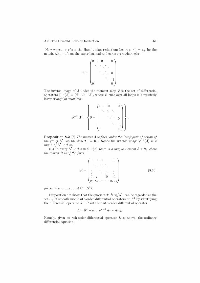
A.8. The Drinfeld–Sokolov Reduction 261
Now we can perform the Hamiltonian reduction: Let Λ ∈ n∗− = n+ be the
matrix with −1’s on the superdiagonal and zeros everywhere else:
Λ :=
⎛
⎜
⎜
⎜
⎜
⎜
⎜
⎜
⎝
0 −1 0 0. . . . . . . . .
. . . . . . 0. . . −1
0 0
⎞
⎟
⎟
⎟
⎟
⎟
⎟
⎟
⎠
.
The inverse image of Λ under the moment map Φ is the set of differentialoperators Φ−1(Λ) = ∂ + B + Λ, where B runs over all loops in nonstrictlylower triangular matrices:
Φ−1(Λ) =
⎧
⎪
⎪
⎪
⎪
⎪
⎪
⎪
⎨
⎪
⎪
⎪
⎪
⎪
⎪
⎪
⎩
∂ +
⎛
⎜
⎜
⎜
⎜
⎜
⎜
⎜
⎝
∗ −1 0 0. . . . . . . . .
. . . . . . 0. . . −1
∗ ∗
⎞
⎟
⎟
⎟
⎟
⎟
⎟
⎟
⎠
⎫
⎪
⎪
⎪
⎪
⎪
⎪
⎪
⎬
⎪
⎪
⎪
⎪
⎪
⎪
⎪
⎭
.
Proposition 8.2 (i) The matrix Λ is fixed under the (conjugation) action ofthe group N− on the dual n∗
− = n+. Hence the inverse image Φ−1(Λ) is aunion of N−-orbits.
(ii) In every N−-orbit in Φ−1(Λ) there is a unique element ∂ + R, wherethe matrix R is of the form
R =
⎛
⎜
⎜
⎜
⎜
⎜
⎜
⎝
0 −1 0 0. . . . . . . . .
.... . . . . . 0
0 . . . 0 −1u0 u1 · · · · · · un−1
⎞
⎟
⎟
⎟
⎟
⎟
⎟
⎠
(8.30)
for some u0, . . . , un−1 ∈ C∞(S1).
Proposition 8.2 shows that the quotient Φ−1(Λ)/N− can be regarded as theset Ln of smooth monic nth-order differential operators on S1 by identifyingthe differential operator ∂ +R with the nth-order differential operator
L = ∂n + un−1∂n−1 + · · · + u0 .
Namely, given an nth-order differential operator L as above, the ordinarydifferential equation
262 Appendices
Lψ = 0
of order n is equivalent to the system of first-order differential equations
∂Ψ +RΨ = 0 ,
where R is the matrix of type (8.30) and Ψ is a vector-solution, Ψ =(ψ0, . . . , ψn−1)t. The equivalence of the two equations comes from settingψ0 := ψ. Then the first n − 1 equations of the system imply ψ1 :=ψ′, . . . , ψn−1 := ψ(n−1), while the last equation of the system reads ψ(n) +un−1ψ
(n−1) + · · · + u0ψ = 0, i.e., Lψ = 0.Return to the whole affine space ∂ + A | A ∈ Lgln of all matrix differ-
ential operators, regarded as a hyperplane in the smooth dual of the affineLie algebra Lgln. It carries a natural Poisson structure, which is the linearLie–Poisson structure on the dual Lgln
∗, restricted to this hyperplane. This
linear Poisson structure produces a certain Poisson structure on the symplec-tic quotient Φ−1(Λ)/N− as a result of the Hamiltonian reduction; see SectionI.5. The theorem of Drinfeld and Sokolov states that this Poisson structurecoincides with the quadratic Gelfand–Dickey Poisson structure on the spaceLn = L of (monic) nth-order differential operators L:
Theorem 8.3 (Drinfeld–Sokolov [88]) The Poisson structure on the quo-tient Φ−1(Λ)/N− coincides with the quadratic (or second) Gelfand–Dickeystructure on the space Ln of smooth monic nth-order differential operators onthe circle.
We refer to the original paper [88] or to the book [80] for a proof by directcalculation. Below we shall prove this fact using ideas from the Poisson Liegroups combined with the approach in [115].
Remark 8.4 The linear (or first) Gelfand–Dickey structure can also be ob-tained by the Hamiltonian reduction from the smooth dual of the affine Liealgebra Lgln. Just as the quadratic Gelfand–Dickey structure is obtained fromthe reduction of the linear Lie–Poisson structure on Lgln
∗, the linear Gelfand–
Dickey structure comes from a constant Poisson structure on Lgln
∗. Details
on how to choose the freezing point and to perform the reduction can befound, for example, in [88, 31]. The Drinfeld–Sokolov reduction has also beengeneralized to pseudodifferential symbols of arbitrary complex degree α ∈ C
in [191]. In this case, the matrix algebra gln is replaced by the “Lie algebraof matrices of complex size α × α,” which was introduced by Feigin in [116].A q-analogue of the universal Drinfeld–Sokolov reduction for complex degreesis described in [314]. There is also a version of the Drinfeld–Sokolov reductionassociated to any simple subalgebra of gln [88].
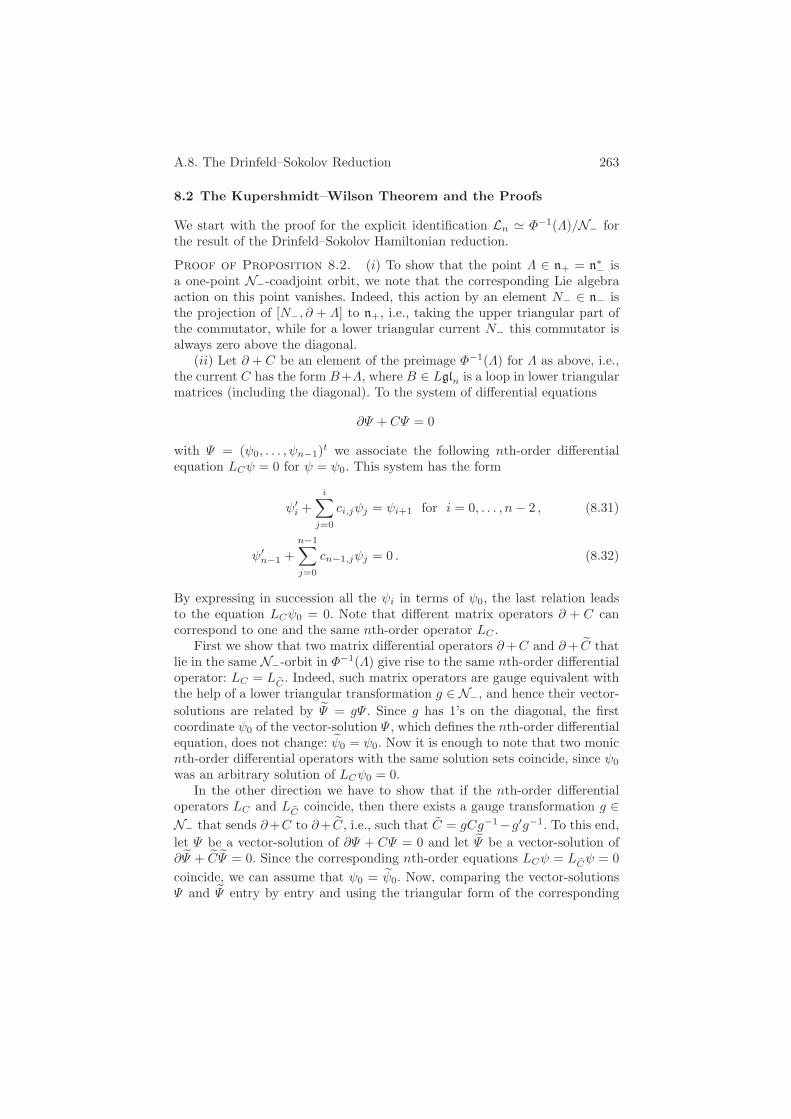
A.8. The Drinfeld–Sokolov Reduction 263
8.2 The Kupershmidt–Wilson Theorem and the Proofs
We start with the proof for the explicit identification Ln Φ−1(Λ)/N− forthe result of the Drinfeld–Sokolov Hamiltonian reduction.
Proof of Proposition 8.2. (i) To show that the point Λ ∈ n+ = n∗− is
a one-point N−-coadjoint orbit, we note that the corresponding Lie algebraaction on this point vanishes. Indeed, this action by an element N− ∈ n− isthe projection of [N−, ∂ + Λ] to n+, i.e., taking the upper triangular part ofthe commutator, while for a lower triangular current N− this commutator isalways zero above the diagonal.
(ii) Let ∂ + C be an element of the preimage Φ−1(Λ) for Λ as above, i.e.,the current C has the form B+Λ, where B ∈ Lgln is a loop in lower triangularmatrices (including the diagonal). To the system of differential equations
∂Ψ + CΨ = 0
with Ψ = (ψ0, . . . , ψn−1)t we associate the following nth-order differentialequation LCψ = 0 for ψ = ψ0. This system has the form
ψ′i +
i∑
j=0
ci,jψj = ψi+1 for i = 0, . . . , n− 2 , (8.31)
ψ′n−1 +
n−1∑
j=0
cn−1,jψj = 0 . (8.32)
By expressing in succession all the ψi in terms of ψ0, the last relation leadsto the equation LCψ0 = 0. Note that different matrix operators ∂ + C cancorrespond to one and the same nth-order operator LC .
First we show that two matrix differential operators ∂+C and ∂+ ˜C thatlie in the same N−-orbit in Φ−1(Λ) give rise to the same nth-order differentialoperator: LC = L
˜C . Indeed, such matrix operators are gauge equivalent withthe help of a lower triangular transformation g ∈ N−, and hence their vector-solutions are related by ˜Ψ = gΨ . Since g has 1’s on the diagonal, the firstcoordinate ψ0 of the vector-solution Ψ , which defines the nth-order differentialequation, does not change: ˜ψ0 = ψ0. Now it is enough to note that two monicnth-order differential operators with the same solution sets coincide, since ψ0
was an arbitrary solution of LCψ0 = 0.In the other direction we have to show that if the nth-order differential
operators LC and L˜C coincide, then there exists a gauge transformation g ∈
N− that sends ∂+C to ∂+ ˜C, i.e., such that C = gCg−1−g′g−1. To this end,let Ψ be a vector-solution of ∂Ψ + CΨ = 0 and let ˜Ψ be a vector-solution of∂ ˜Ψ + ˜C ˜Ψ = 0. Since the corresponding nth-order equations LCψ = L
˜Cψ = 0coincide, we can assume that ψ0 = ˜ψ0. Now, comparing the vector-solutionsΨ and ˜Ψ entry by entry and using the triangular form of the corresponding

264 Appendices
equations (8.31) they satisfy, we find that the transformation from Ψ to ˜Ψ
is also lower triangular with 1’s on the diagonal: ˜Ψ = gΨ for g ∈ N−. Thisimplies that ∂ + C and ∂ + ˜C lie in the same N−-orbit in Φ−1(Λ).
Before proving the Drinfeld–Sokolov theorem we are going to derive the“multiplicative” property of the quadratic Gelfand–Dickey bracket known asthe Kupershmidt–Wilson theorem.
For this purpose, consider the space of the first-order scalar differentialoperators L1 := L = ∂ + v | v ∈ C∞(S1). We define the following constantPoisson bracket on the space of such operators (and discuss the origin for thisPoisson structure a little later). Namely, if F (v) and G(v) are two functionalson the space L1, their Poisson bracket is
F,G(v) :=∫
S1
δF
δv
(
δG
δv
)′dθ ,
where δF/δv is the variational derivative of F . This bracket is a constantPoisson bracket on L1 (cf. Definition I.4.20): the corresponding contractionof the variational derivatives does not depend on v itself. The Hamiltonianvector field on L1 corresponding to a linear functional Ff (v) :=
∫
f · v dθassumes the value Vf (L) := −f ′ at L = ∂ + v.
Consider now the product L1 × · · · ×L1 → Ln of several first-order differ-ential operators to obtain one nth-order differential operator:
((∂ + vn−1), . . . , (∂ + v0)) → L = (∂ + vn−1) · · · (∂ + v0)
= ∂n + un−1∂n−1 + · · · + u0 .
Definition 8.5 The map vi → uj given by the product of differentialoperators L1 × · · · × L1 → Ln is called the Miura transformation.
Theorem 8.6 (Kupershmidt–Wilson [226]) The Miura transformationsends the constant Poisson bracket on the product L1 × · · · × L1 of first-order operators to the quadratic Gelfand–Dickey bracket on the space Ln ofnth-order differential operators.
Proof. Recall that both the spaces L1 and Ln are Poisson submanifolds inthe Poisson Lie group ˜GINT of pseudodifferential symbols. In turn, the groupmultiplication on any Poisson Lie group maps the Poisson structure on thesquare of this group to the Poisson structure of this group itself. For the group˜GINT this implies that the Gelfand–Dickey bracket restricted to (several copiesof) the Poisson submanifolds L1 is mapped by the group product, which is themultiplication of differential operators, to the Gelfand–Dickey bracket on Ln.
Now the theorem follows from the observation that the quadratic Gelfand–Dickey structure restricted to the first-order operators L1 drastically simplifies

A.8. The Drinfeld–Sokolov Reduction 265
and becomes exactly the constant Poisson bracket discussed above. In orderto see the latter we consider a cotangent vector X = ∂−1a to the space offirst-order differential operators L = ∂ + v. Then the corresponding Gelfand–Dickey Hamiltonian field V 2
X(L) is given by
V 2X(L) = (L X)+ L− L (X L)+ = −a′ ,
which is exactly the Hamiltonian field in the constant Poisson bracketabove.
Remark 8.7 The Hamiltonian property of the Miura map is important inintegrable systems. For instance, for n = 2 and L = ∂2 + u = (∂ − v)(∂ + v)the Miura map gives u = v′ − v2. If the function u satisfies the KdV equationut = −3uu′ − (1/2)u′′′, then the function v satisfies the so called modifiedKdV (or m-KdV) equation vt = 3v2v′ − (1/2)v′′′.
Now we are ready to prove the Drinfeld–Sokolov reduction theorem.
Proof of Theorem 8.3. We would like to show that the linear Lie–Poisson structure descends from Lgln
∗to the quadratic Poisson structure on
the quotient of Φ−1(Λ) over the N−-action:
Φ−1(Λ)/N− ∂ +R = Ln .
For this purpose we take an auxiliary step: we first restrict the linear Poissonbracket from Lgln
∗not to Φ−1(Λ), but to a certain subspace, and after that
we take the quotient from this subspace to ∂ +R.This auxiliary (affine) subspace ∂ +P ⊂ Φ−1(Λ) consists of all currents
P of the form
P =
⎛
⎜
⎜
⎜
⎜
⎜
⎜
⎜
⎝
v0 −1 0 0
0. . . . . . . . .. . . . . . . . . 0
. . . . . . −10 0 vn−1
⎞
⎟
⎟
⎟
⎟
⎟
⎟
⎟
⎠
. (8.33)
This subspace has the “same functional dimension” as Ln. (Note, however,that this subspace is not a section for the fibration Φ−1(Λ) → Ln given by theN−-action: different operators ∂ + P can belong to the same N−-orbit andthen correspond to the same differential operator ∂+R, as we discuss below.)
The restriction of the linear Lie–Poisson structure from Lgln
∗to this sub-
space can be found explicitly.
Exercise 8.8 Verify that the linear Lie–Poisson structure from Lgln
∗re-
stricted to the subspace ∂ + P gives the constant Poisson structure on the

266 Appendices
coefficients vj discussed above. (Hint: the Lie–Poisson bracket on this sub-space is equivalent to the Lie structure on the centrally extended subalgebraof loops in diagonal matrices under the identification we considered. The onlynontrivial term in the commutator between such “diagonal currents” comesfrom the 2-cocycle. Finally, the affine 2-cocycle restricted to the diagonal partcan be thought of as the sum of several Lgl1-cocycles c(a, b) =
∫
S1(a · b′) dθ.The latter Lie algebra is an infinite-dimensional Heisenberg algebra, and itcorresponds to the constant Poisson bracket discussed above; see details in[115].)
Now we note that this subspace ∂ + P can be rewritten as the spaceof nth-order differential operators L expressed as products of first-orderoperators
L = (∂ + vn−1) · · · (∂ + v0) .
Indeed, the system of first-order differential equations (∂ + P )Ψ = 0 for avector-solution Ψ = (ψ0, . . . , ψn−1)t is equivalent to the scalar differentialequation Lψ = 0 under an identification similar to the one above. Namely,we set ψ0 := ψ, which forces ψ1 := (∂ + v0)ψ0, ψ2 := (∂ + v1)ψ1 etc., while(∂ + vn−1)ψn−1 = 0.
Thus the passage to the quotient ∂ + P → ∂ + R = Ln is the Miuratransform, and the Kupershmidt–Wilson theorem completes the proof: theconstant Poisson bracket on ∂ + P becomes the quadratic Gelfand–Dickeybracket on Ln = Φ−1(Λ)/N−.
A.9. The Lie Algebra gl∞ 267
A.9 The Lie Algebra gl∞
In this section we introduce yet another Lie algebra, gl∞, along with its centralextension gl∞, which connects some of the algebras we encountered through-out the book. In particular, the extended Lie algebra gl∞ contains as subalge-bras the Virasoro algebra, the centrally extended Lie algebra DO of differentialoperators on the circle, and the affine Lie algebras Lgln for all n ∈ N.
9.1 The Lie Algebra gl∞ and Its Subalgebras
Definition 9.1 The space gl∞ consists of doubly infinite matrices that canhave nonzero entries only inside a strip of finite width around the maindiagonal:
gl∞ = A = (aij)i,j∈Z | ∃ N such that aij = 0 for all i, j with |i− j| > N .
The multiplication of two such matrices is well defined, since for the productC = AB of two matrices A,B ∈ gl∞, the sum cij =
∑
k aikbkj is finite. TheLie algebra gl∞ is the above space equipped with the Lie bracket [A,B] =AB −BA.
This large Lie algebra has many interesting subalgebras.
Example 9.2 (Differential operators on the circle) Consider the spaceC[z, z−1] of Laurent polynomials with coefficients in C. This space can beidentified with the space of vectors X = (xi)i∈Z of infinite length with onlyfinitely many nonzero entries. The Lie algebra gl∞ acts naturally on the latterspace by left multiplication. In this identification, the derivative operator z d
dzis identified with the diagonal matrix D = (dij), where dii = i for all i ∈ Z,and dij = 0 for all i = j. Furthermore, the operator Z of multiplication bythe monomial z on C[z, z−1] is given by the shift matrix, which has ones onthe superdiagonal and zeros everywhere else: Z = (aij) with ai i+1 = 1 andaij = 0 for all i, j with j = i+ 1. Similarly, the operator Z−1 is given by thematrix that has ones on the subdiagonal and zeros everywhere else.
The subspace in gl∞ generated by sums and compositions of the operatorsD and Z realizes the Lie algebra of polynomial differential operators on thecircle as a subalgebra of gl∞. (We restrict our attention to differential opera-tors whose coefficients are Laurent polynomials, instead of smooth functionson the circle, in order to avoid convergence issues.) As before, one can use themap z → eiθ to identify the operator iz d
dz with the usual derivative operator∂θ on the circle.
Note that the above embedding of differential operators to gl∞ does notextend to an embedding of (polynomial) pseudodifferential symbols. Indeed,in the identification described above, the inverse ∂−1
θ of the derivative operator∂θ cannot be realized inside gl∞: the matrix D = (dij) with dii = i has a zerorow and is not invertible.

268 Appendices
Fig. 9.1. Matrices in gl∞, the operator D realizing z ddz
, and the operator Z formultiplying by z.
Example 9.3 (Loop algebras inside gln) Fix some integer n ∈ N. We callan element A = (aij)i,j∈Z ∈ gl∞ periodic of order n if ai+n,j+n = ai,j forall i, j ∈ Z. The subalgebra of all periodic elements of order n can be iden-tified with the algebra gln ⊗ C[z, z−1] of polynomial loops in gln. Indeed, aperiodic matrix A of order n is completely determined by fixing the n rows(aij)0≤i<n,j∈Z. Associate to the periodic matrix A the sequence of n× n ma-trices Ak, k ∈ Z, by Ak := (aij), where 0 ≤ i < n and kn ≤ j < (k+1)n. Notethat only a finite number of the matrices Ak can be nonzero. We identify sucha sequence with the Laurent series
∑
k Akzk. This gives a bijection between
the set of periodic matrices of order n in gl∞ and polynomial loop algebra(Lgln)pol = gln ⊗ C[z, z−1].
Exercise 9.4 Show that the bijection between the set of periodic matrices oforder n in gl∞ and the loop algebra (Lgln)pol described above defines a Liealgebra isomorphism.
9.2 The Central Extension of gl∞
Let J be the diagonal matrix defined by jii = −1 if i ≥ 0, and jii = 1 if i < 0.
Exercise 9.5 Given two elements A,B ∈ gl∞, show that the matrix C :=[J,A]B has only finitely many nonzero entries on the diagonal. (Hint: seeFigure 9.2.)
A [J,A]
Fig. 9.2. For every matrix A ∈ gl∞, the commutation with J “cuts out” the upperleft and lower right quadrants of A and multiplies the off-diagonal elements by ±2.

A.9. The Lie Algebra gl∞ 269
Definition 9.6 The central extension gl∞ of the Lie algebra gl∞ is definedby the 2-cocycle
(A,B) =12
tr([J,A], B) . (9.34)
This cocycle has appeared in a series of papers [75] related to solitonequations and related algebraic constructions, and it is often referred to asthe Japanese cocycle.
Proposition 9.7 (i) When restricted to the Lie subalgebra DO ⊂ gl∞ ofpolynomial differential operators, the cocycle is cohomologous to (a multipleof) the Kac–Peterson 2-cocycle. In particular, restricted to the Lie algebra ofvector fields on the circle, is cohomologous to (a multiple of) the Gelfand–Fuchs 2-cocycle.
(ii) Restricted to the subalgebra (Lgln)pol ⊂ gl∞, the cocycle coincideswith the cocycle defining the affine Lie algebra ( Lgln)pol.
In particular, the 2-cocycle is nontrivial on gl∞, and gl∞ is a nontrivialcentral extension of the latter algebra.
Exercise 9.8 Give a proof of Proposition 9.7. (Hint: For part (i) it is enoughto prove the assertion for vector fields. Show that in the basis Ln = zn+1 d
dz ,the cocycle has the explicit form
(Ln, Lm) = δn,−m
n∑
i=1
i(i− 1) .
For part (ii) start with the case of gl1, i.e., with ordinary Laurent polynomials.The general case is similar.)
Corollary 9.9 The Virasoro algebra, the centrally extended Lie algebra DO,as well as all the affine Lie algebras ( Lgln)pol, are Lie subalgebras of gl∞.
Remark 9.10 There is a generalization of gl∞ in which the strip can beunbounded downward: one requires only that aij = 0 for all i, j satisfyingj − i > N , rather than |i − j| > N . The multiplication, the Lie bracket, andthe 2-cocycle are still well defined on the space of such matrices.
9.3 q-Difference Operators and gl∞
Other interesting subalgebras of gl∞ are the algebras of q-versions of differen-tial operators and pseudodifferential symbols. Consider the “shift operator”Dq on the space C[z, z−1] of Laurent polynomials: Dqf(z) := f(qz). Note thatthe finite difference operator
270 Appendices
∂q :=Dq − 1q − 1
becomes the derivative operator z∂z in the limit q → 1, since (f(qz)−f(z)/(q−1) → zf ′(z). Thus the operator (Dq − 1)/(q − 1) (or the operator Dq itself)can be regarded as a quantum version of the derivative operator. The operatorDq also satisfies the q-analogue of the Leibniz rule Dq f = (Dqf)Dq, similarto that for the derivative.
Now one can define the algebras of q-difference operators DOq :=∑n
0 uk(z)Dkq and q-difference symbols ψDSq :=
∑n−∞ uk(z)Dk
q . (Oneusually assumes that q is not a root of unity, i.e., qn = 1 for any n, to avoidextra relations of (Dn
q = 1)-type.)Furthermore, one can define the notion of logDq for the algebra of q-
difference symbols, and it turns out to have a very simple meaning. Since Dq
is a shift operator, one can think of it as the exponent of the derivative operatorDq = exp(q · z∂z); cf. Section II.4.2. Then logDq is the derivative operatorq · z∂z itself! Note that the derivative z∂z does not belong to the algebra ofq-difference symbols, and it defines an outer derivation of the algebra ψDSq.One can proceed by defining the corresponding 2-cocycles, constructing theLie group of fractional q-difference symbols, and the corresponding integrablesystems; see [190, 313].
The trace on q-difference symbols is defined by Trq(∑
uk(z)Dkq ) := tr(u0),
where tr(u0) is the constant term in the Laurent polynomial u0(z), i.e., itscoefficient at z0. It is an algebraic trace, since it satisfies Trq[A,B] = 0,similar to the trace on pseudodifferential symbols. One should note, however,that the subalgebras of positive and negative powers of Dq are not isotropicwith respect to the quadratic form related to this trace on ψDSq, and thusthey do not form a Manin triple. Although the corresponding Lie group is nota Poisson Lie group, it can still be equipped with a natural Poisson structure[313, 314].
Finally, we note that the algebras DOq and ψDSq act on the space ofLaurent polynomials C[z, z−1], and hence their action can be defined by infi-nite matrices. One can easily see that the generators of ψDSq are described bymatrices “of finite width,” i.e., they belong to gl∞. This gives an embeddingof ψDSq as a subalgebra of gl∞; see, e.g., [180].
Remark 9.11 The Lie algebra gl∞ and its central extension gl∞ by meansof the cocycle have a long history and have been used to study the KdVequation, the KP hierarchy, and other integrable hierarchies (see, e.g., [372,181] and references therein).
Among various relations between gl∞ and other algebras, including ψDSq,it is worth mentioning that the algebra ψDSq is also isomorphic to the so-called noncommutative torus: the associative algebra generated by two unitaryoperators U1 and U2 satisfying the relations U2U1 = qU1U2 for q = eih; see[147, 180].
A.9. The Lie Algebra gl∞ 271
Another interesting version of this algebra is known as the sine algebra[111, 146, 147]. One can also think of it as an algebra with continuous rootsystems, as was defined in [335]. Finally, the limit of the structure constantsof the sine algebra gives those of the Lie algebra SVect(T 2) of divergence-free vector fields on the two-dimensional torus [320, 49]. In this way, thealgebra gl∞ provides a link to a number of the infinite-dimensional Lie algebrasconsidered in this book. We also refer the interested reader to [118] for manyother related constructions.

272 Appendices
A.10 Torus Actions on the Moduli Space of FlatConnections
Let G be a compact or complex simple Lie group. In this appendix we discussa torus action on the moduli space of flat connections on the trivial G-bundleover a Riemann surface Σ. We start with constructing a natural set of Poissoncommuting functions on the moduli space of flat connections, and then turnto the case of G = SU(2), where this set of commuting functions gives riseto integrable systems on the symplectic leaves of the moduli space [175]. Thisaction allows one to study the symplectic geometry of the leaves. Finally, fol-lowing [120, 125], we consider the moduli space of flat SL(n,C)-connections onthe one-holed torus and show that the rational Ruijsenaars–Schneider systemlives on a holomorphic symplectic leaf of this moduli space.
10.1 Commuting Functions on the Moduli Space
Let Σ be a compact Riemann surface of genus κ with d boundary components.Here we assume that G is a simply connected simple Lie group with the Liealgebra g. Denote by
AΣ = d+A | A ∈ Ω1(Σ, g)
the affine space of connections in the trivial G-bundle over the surface Σ. Wehave seen in Section III.2.1 that the space AΣ is an infinite-dimensional sym-plectic manifold with a Hamiltonian action of (the central extention GΣ of)the group GΣ = C∞(Σ,G) of gauge transformations. The moment map of thisaction is given by the curvature together with the restriction of the connectionto the boundary ∂Σ (see Proposition III.2.10 for the exact formulation). Thecorresponding symplectic quotient is the moduli space
MΣ = AΣflat/ G
Σ
of flat connections on Σ. This is a finite-dimensional, possibly singular, Pois-son manifold. The symplectic leaves of MΣ are parametrized by fixing theconjugacy classes of the holonomies around the boundary circles of the surfaceΣ. (More precisely, in Section III.2.1 we considered the case of a compact Liegroup G. But all we really need in the constructions is a nondegenerate invari-ant bilinear form on the Lie algebra g. In particular, we can take G to be anysemisimple Lie group, in which case MΣ denotes the space of representationsRep(π1(Σ) → G) modulo conjugation.)
A natural class of functions on the moduli space MΣ can be constructed asfollows. Let f : G → C be a conjugation-invariant function on the group, andlet Γ be a simple curve in Σ. Associate to them the function fΓ : MΣ → C
by assigning to (the equivalence class of) a flat connection A on Σ the valueof f on the holonomy of A around the curve Γ :

A.10. Torus Actions on the Moduli Space of Flat Connections 273
fΓ ([A]) = f(holΓ (A)) .
Goldman gave a formula for the Poisson bracket fΓ1 , gΓ2 in terms of theintersection number of the curves Γ1 and Γ2; see [145]. Here we need only thefollowing special case.
Proposition 10.1 (i) Let Γ1 and Γ2 be two simple disjoint curves on thesurface Σ. Then for any two conjugation-invariant functions f and g on thegroup G, we have
fΓ1 , gΓ2 = 0 .
(ii) For any simple closed curve Γ and any two conjugation-invariant func-tions f and g on the group G, we have
fΓ , gΓ = 0 .
A trinion (or a pair of pants) is a Riemann surface of genus 0 with threeboundary components. Recall that the genus of the Riemann surface Σ isdenoted by κ, and the number of boundary components is d. From now on weassume that d ≥ 1 if κ = 1, and d ≥ 3 if κ = 0. In these cases the Riemannsurface Σ has a trinion decomposition into 2κ−2+d trinions; see Figure 10.1.
Fig. 10.1. A trinion decomposition of a Riemann surface with boundary.
This can be achieved by cutting Σ along 3κ − 3 + d disjoint curves. Onthe other hand, the number of independent conjugation-invariant functionson the group G is equal to its rank rk(G), i.e., to the dimension of a maximaltorus T ⊂ G. Hence, the trinion decomposition of the surface Σ provides uswith (3κ − 3 + d) · rk(G) independent Poisson-commuting functions on themoduli space MΣ . For a closed surface Σ (i.e., for d = 0), the moduli spaceMΣ is symplectic of dimension (2κ − 2) · dim(G). The above functions fΓ
form an integrable system on the moduli space MΣ whenever the numberof independent functions is equal to half the dimension of MΣ , which for aclosed surface happens exactly if dim(G)/ rk(G) = 3. For simple groups thisoccurs only for G = SU(2).
274 Appendices
10.2 The Case of SU(2)
Define a maximal torus T of the group SU(2) as the set of diagonal matrices
T =(
eiθ 00 e−iθ
)
∼= S1 .
Each element of SU(2) is conjugate to an element of the torus T . Furthermore,the matrices diag(eiθ, e−iθ) and diag(e−iθ, eiθ) are conjugate to each other,so that a conjugacy class of SU(2) is completely determined by the tracetr(diag(eiθ, e−iθ)) = 2 cos θ. The centralizers of the corresponding conjugacyclasses are given by the torus T if θ ∈ πZ. Otherwise, the centralizer is thewhole group SU(2).
Recall that for a surface Σ with boundary a symplectic leaf in the modulispace MΣ is singled out by fixing conjugacy classes of the holonomies aroundthe boundary components of Σ.
Proposition 10.2 Let θ1, . . . , θd ∈ [0, π] be such that for all εj ∈ ±1, wehave
∑
εjθj = 0 mod 2π. Then the symplectic leaf defined by the conjugacyclasses of the diagonal matrices diag(eiθj , e−iθj ), j = 1, . . . , d, is a smoothsymplectic manifold of dimension 6κ− 6 + 2d.
Let Γ1, . . . , Γ3κ−3+d denote curves cutting the surface Σ into a triniondecomposition and denote by ˜Γ1 . . . , ˜Γd the boundary circles of the surface Σ.Let φj be the functions on the moduli space MΣ defined by
φj([A]) := cos−1
(
12
tr(holΓj(A))
)
,
and similarly for ˜φk and ˜Γk. By Proposition 10.1, the functions φj and ˜φk allPoisson commute. Consider the map
Φ = (φ1, . . . , φ3κ−3+d, ˜φ1, . . . , ˜φd) : MΣ → R3κ−3+2d .
Jeffrey and Weitsman showed that the restriction of the map Φ to the openand dense subset
MΣ :=
3κ−3+d⋂
j=1
φ−1j (0, π) ∩
d⋂
k=1
˜φ−1k (0, π) ⊂ MΣ
is the moment map of the Hamiltonian action of a (3κ − 3 + d)-dimensionaltorus [174]. This action is given by the twist flows defined as follows.
Denote by Pl, l = 1, . . . , 2κ − 2 + d, the trinions in the above triniondecomposition of the surface Σ with the cutting curves Γj and boundarycurves ˜Γk.

A.10. Torus Actions on the Moduli Space of Flat Connections 275
Definition 10.3 A connection A ∈ AΣ is said to be adapted to the triniondecomposition if around each Γj , there exists a tubular neighborhood Γj ×[−1, 1] such that A|Γj×[−1,1] can be written as
A|Γj×[−1,1] = Xj dθj ,
where Xj is an element of the Lie algebra h = Lie(T ), and dθj is the coordinate1-form on the circle Γj . Furthermore, we require the existence of a (semi-)neighborhood ˜Γk × [−1, 0] of each of the boundary circles such that
A|˜Γk×[−1,0] = ˜Xk d˜θk
with ˜Xk and d˜θk as above.
Exercise 10.4 Show that every flat connection A ∈ AΣflat is gauge-equivalent
to a connection adapted to the trinion decomposition.
To define an action of the torus T 3κ−3+2d ∼= R3κ−3+2d/Z3κ−3+2d on the
moduli space MΣ we fix an element
t := (t1, . . . , t3κ−3+d,˜t1, . . . ,˜td) ∈ T 3κ−3+2d
and take an element
(ψ1, . . . , ψ2κ−2+d) ∈2κ−2+d∏
l=1
GPl
in the product of the corresponding current groups, such that the restrictionsof ψl to different (semi-) neighborhoods of Γj and ˜Γk are given by
ψl|Γj×[0,1] = tj , ψl|Γj×[−1,0] = id, and ψl| ˜Γk×[−1,0] = ˜tk
whenever any of the semi-neighborhoods Γj×[0, 1], Γj×[−1, 0], and ˜Γk×[−1, 0]belongs to the pair of pants Pl. Such an element (ψ1, . . . , ψ2κ−2+d) acts onthe set of connections that are adapted to the trinion decomposition by thegauge action on each piece Pl:
A|Pl→ A|Pl
:= ψl ·A|Pl· ψ−1
l − dψl · ψ−1l .
Indeed, the gauge transformation ψl does not change A|Plin a neighborhood
of the boundary of the trinion Pl, so that all A|Plfit together to form a
connection A on the surface Σ. This action descends to an action of theelement t ∈ T 3κ−3+2d on the moduli space MΣ , since any two choices of(ψ1, . . . , ψ2κ−2+d) for the same t differ by an element of the current group GΣ .The action of the torus T 3κ−3+2d preserves the holonomies of the connectionA around the circles Γj and ˜Γk, and hence preserves the fibers of the map Φ.
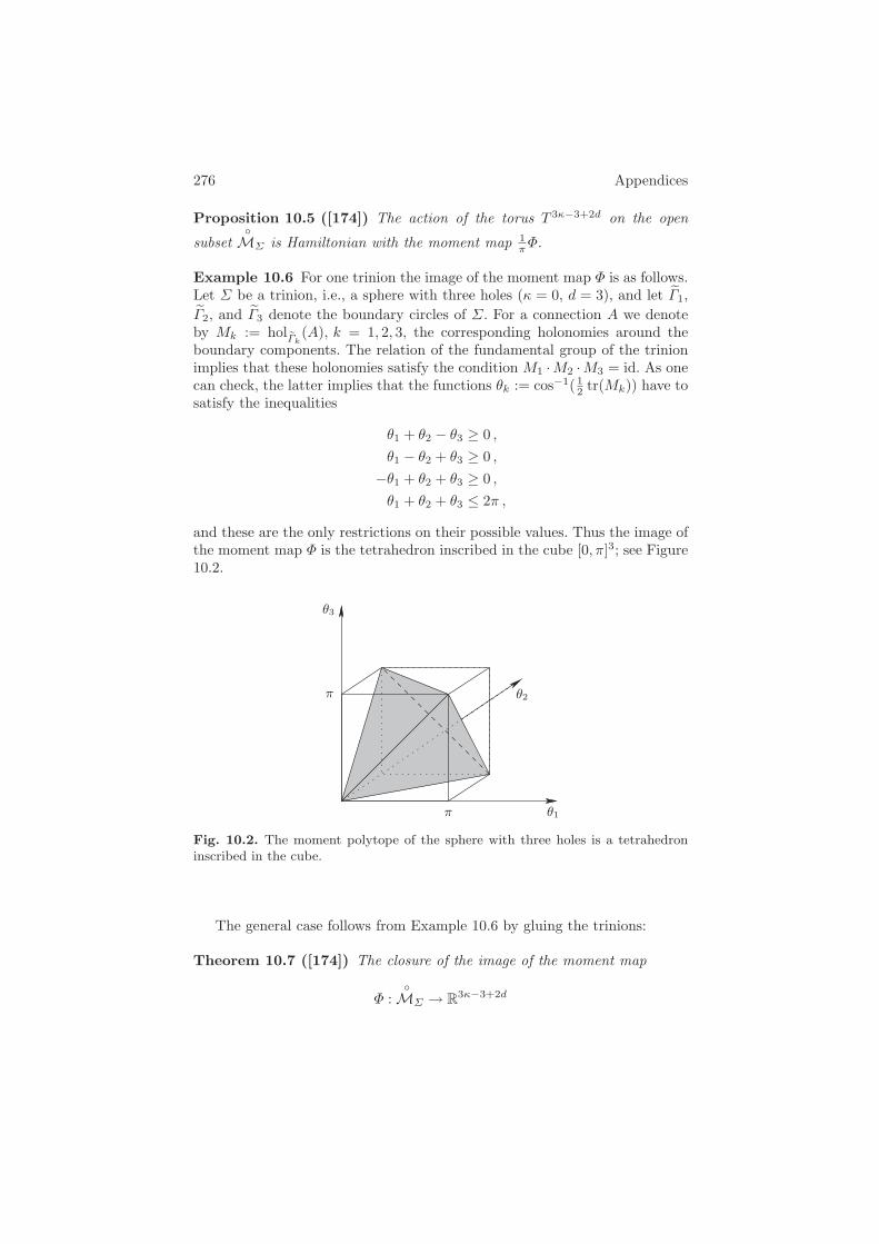
276 Appendices
Proposition 10.5 ([174]) The action of the torus T 3κ−3+2d on the open
subset
MΣ is Hamiltonian with the moment map 1πΦ.
Example 10.6 For one trinion the image of the moment map Φ is as follows.Let Σ be a trinion, i.e., a sphere with three holes (κ = 0, d = 3), and let ˜Γ1,˜Γ2, and ˜Γ3 denote the boundary circles of Σ. For a connection A we denoteby Mk := hol
˜Γk(A), k = 1, 2, 3, the corresponding holonomies around the
boundary components. The relation of the fundamental group of the trinionimplies that these holonomies satisfy the condition M1 ·M2 ·M3 = id. As onecan check, the latter implies that the functions θk := cos−1( 1
2 tr(Mk)) have tosatisfy the inequalities
θ1 + θ2 − θ3 ≥ 0 ,θ1 − θ2 + θ3 ≥ 0 ,
−θ1 + θ2 + θ3 ≥ 0 ,θ1 + θ2 + θ3 ≤ 2π ,
and these are the only restrictions on their possible values. Thus the image ofthe moment map Φ is the tetrahedron inscribed in the cube [0, π]3; see Figure10.2.
π
π
θ3
θ1
θ2
Fig. 10.2. The moment polytope of the sphere with three holes is a tetrahedroninscribed in the cube.
The general case follows from Example 10.6 by gluing the trinions:
Theorem 10.7 ([174]) The closure of the image of the moment map
Φ :
MΣ → R3κ−3+2d
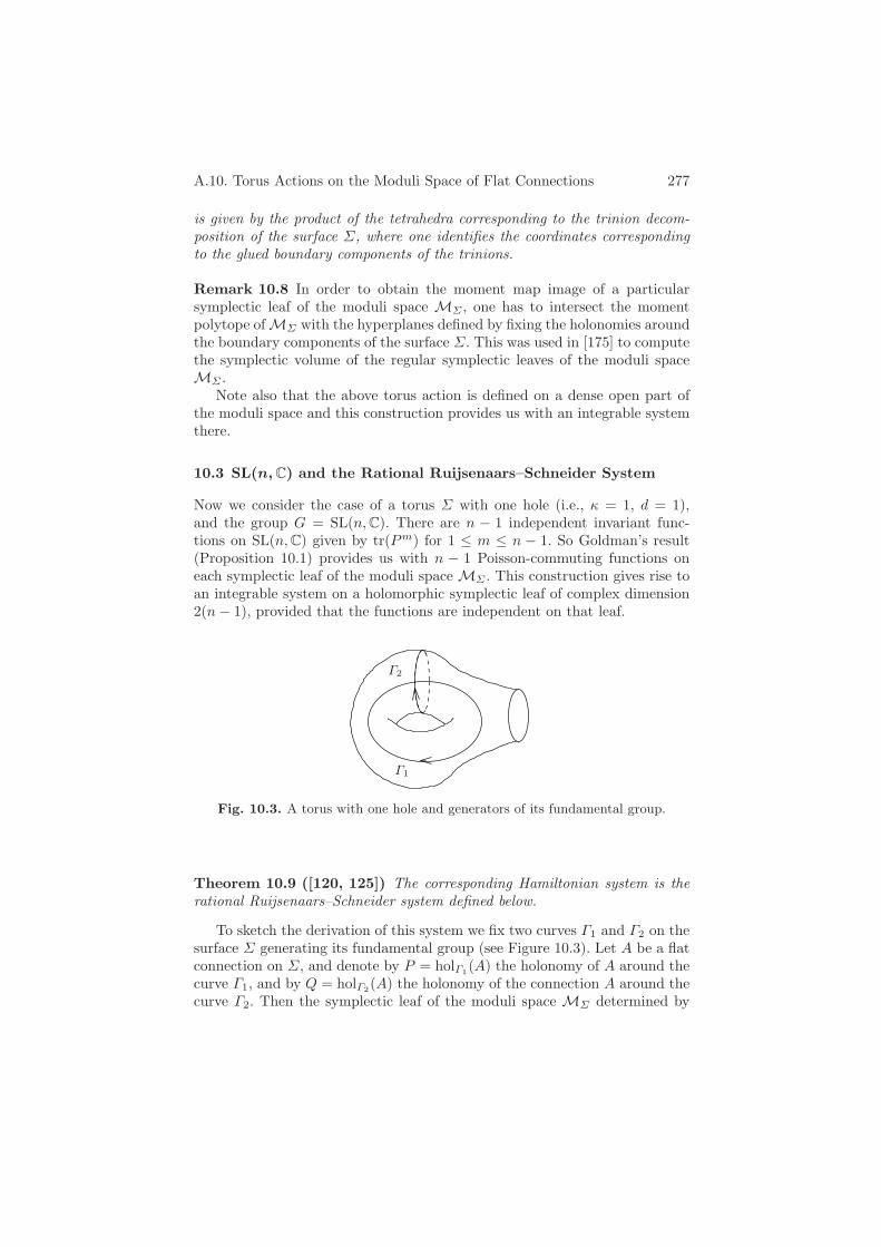
A.10. Torus Actions on the Moduli Space of Flat Connections 277
is given by the product of the tetrahedra corresponding to the trinion decom-position of the surface Σ, where one identifies the coordinates correspondingto the glued boundary components of the trinions.
Remark 10.8 In order to obtain the moment map image of a particularsymplectic leaf of the moduli space MΣ , one has to intersect the momentpolytope of MΣ with the hyperplanes defined by fixing the holonomies aroundthe boundary components of the surface Σ. This was used in [175] to computethe symplectic volume of the regular symplectic leaves of the moduli spaceMΣ .
Note also that the above torus action is defined on a dense open part ofthe moduli space and this construction provides us with an integrable systemthere.
10.3 SL(n, C) and the Rational Ruijsenaars–Schneider System
Now we consider the case of a torus Σ with one hole (i.e., κ = 1, d = 1),and the group G = SL(n,C). There are n − 1 independent invariant func-tions on SL(n,C) given by tr(Pm) for 1 ≤ m ≤ n − 1. So Goldman’s result(Proposition 10.1) provides us with n − 1 Poisson-commuting functions oneach symplectic leaf of the moduli space MΣ . This construction gives rise toan integrable system on a holomorphic symplectic leaf of complex dimension2(n− 1), provided that the functions are independent on that leaf.
Γ2
Γ1
Fig. 10.3. A torus with one hole and generators of its fundamental group.
Theorem 10.9 ([120, 125]) The corresponding Hamiltonian system is therational Ruijsenaars–Schneider system defined below.
To sketch the derivation of this system we fix two curves Γ1 and Γ2 on thesurface Σ generating its fundamental group (see Figure 10.3). Let A be a flatconnection on Σ, and denote by P = holΓ1(A) the holonomy of A around thecurve Γ1, and by Q = holΓ2(A) the holonomy of the connection A around thecurve Γ2. Then the symplectic leaf of the moduli space MΣ determined by

278 Appendices
forcing the holonomy of the connection A around the boundary of Σ to lie inthe conjugacy class CX of an a priori fixed matrix X in SL(n,C) is given by
MXΣ = P,Q ∈ SL(n,C) | QPQ−1P−1 ∈ CX/SL(n,C) ,
where SL(n,C) acts on pairs (P,Q) by simultaneous conjugation.A symplectic leaf of complex dimension 2(n − 1) is given by fixing the
matrix X = diag(a, . . . , a, b), where a is any (nonzero) complex number, andb = a−n+1. Indeed, a necessary condition for QPQ−1P−1 to be an element ofthe conjugacy class CX is that
rk(QPQ−1 − aP ) ≤ 1 .
In particular, all 2×2 minors of QPQ−1−aP have to vanish. In a basis whereQ is a diagonal matrix Q = diag(q1, . . . , qn), we have
(QPQ−1 − aP )ij = qiq−1j pij − apij .
Now by using the vanishing condition for the 2 × 2 minors of the matrixQPQ−1 − aP , we obtain
pij =√piipjj(1 − a)
qiq−1j − a
.
This shows that the symplectic leaf MXΣ is 2(n−1)-dimensional: it is fixed by
the parameters (p11, . . . , pnn, q1, . . . , qn) subject to the conditions detP = 1and detQ = 1.
In the new coordinates qi and si, where
si := piia(n−1)/2
⎛
⎝
∏
j, j =i
(qj − qi)(qi − qj)(qj − aqi)(qi − aqj)
⎞
⎠
12
,
the Poisson brackets assume the form
qi, qj =0 ,si, sj =0 ,qi, sj =δijpisj ;
see [120]. The functions si are independent and give rise to an integrablesystem on the symplectic leaf MX
Σ .Finally, consider the Hamiltonian function H(P,Q) = tr(P +P−1) on the
moduli space MXΣ . In terms of the variables qi and si it has the following
explicit form:
H(s, q) =∑
i
(si + s−1i )a
n−12
⎛
⎝
∏
k, k =i
(qk − qi)(qi − qk)(qk − aqi)(qi − aqk)
⎞
⎠
12
,
A.10. Torus Actions on the Moduli Space of Flat Connections 279
where a is a parameter. This is the Hamiltonian of the rational Ruijsenaars–Schneider system [333, 332].
Note that the Hamiltonian H(P,Q) = tr(P + P−1) can be regarded asa group version of the Hamiltonian that appeared in the construction of therational Calogero–Moser system by symplectic reduction (see Section II.5.4).Indeed, by considering matrices P = id + ˜P close to the identity in SL(n,C)one can view the Hamiltonian H(P,Q) = tr(P +P−1) as a deformation of theCalogero–Moser Hamiltonian tr( ˜P 2) + const.
Definition 10.10 The elliptic Ruijsenaars–Schneider system has theHamiltonian
H(p, q) =∑
i
cosh(βpi)
⎛
⎝
∏
k, k =i
(1 − a2℘(a(qi − qk); τ))
⎞
⎠
12
,
which is a relativistic version of the elliptic Calogero–Moser Hamiltonianfunction.
Exercise 10.11 Derive the rational and trigonometric versions of theRuijsenaars–Schneider Hamiltonian from the elliptic one by taking appro-priate limits of the elliptic parameter τ . Compare the rational limit with theHamiltonian above for si = exp(βpi). (Hint: see [332].)


References
1. Adams, J.F., Lectures on Lie Groups, W. A. Benjamin, Inc., New York,Amsterdam, 1969.
2. Adams, M.R., Harnad, J., Hurtubise, J., Liouville generating functions forisospectral flow in loop algebras, in Integrable and Superintegrable Systems,232–256, World Sci. Publ., Teaneck, NJ, 1990.
3. Adler, M., On a trace functional for formal pseudo differential operators andthe symplectic structure of the Korteweg-deVries type equations, Invent. Math.50:3 (1978/79), 219–248.
4. Adler, M., van Moerbeke, P., Completely integrable systems, Euclidean Liealgebras, and curves, Adv. in Math. 38:3 (1980), 267–317.
5. Albeverio, S., Sengupta, A., A mathematical construction of the non-abelianChern-Simons functional integral, Comm. Math. Phys. 186 (1997), 563–579.
6. Alekseev, A.Y., Malkin, A.Z., Meinrenken, E., Lie group valued moment maps,J. Differ. Geom. 48:3 (1998), 445–495.
7. Aleksovsky, V.A., Lukatsky, A.M., Nonlinear dynamics of ferromagnet mag-netization and the motion of a generalized rigid body with a current group,Theoret. and Math. Phys. 85 (1990), 1090–1096.
8. Allison, B. S. Azam, S., Berman, S., Gao, Y., Pianzola, A., Extended affine Liealgebras and their root systems, Mem. Am. Math. Soc., 603 (1997), 1–122.
9. Ambrosio, L., Rigot, S., Optimal mass transportation in the Heisenberg group,J. Funct. Anal. 208 (2004), no. 2, 261–301.
10. Andersen, J.E., Mattes, J., Reshetikhin, N., The Poisson structure on themoduli space of flat connections and chord diagrams, Topology 35:4 (1996),1069–1083.
11. Arnold, V.I., A theorem of Liouville concerning integrable problems of dynam-ics, Sibirsk. Mat. Zh. 4 (1963), 471–474.
12. Arnold, V.I., Sur la geometrie differentielle des groupes de Lie de dimensioninfinie et ses applications a l’hydrodynamique des fluides parfaits, Ann. Inst.Fourier (Grenoble) 16 (1966), 319–361;
13. Arnold, V.I., The Hamiltonian nature of the Euler equation in the dynamics ofa rigid body and of an ideal fluid, Uspekhi Mat. Nauk 24:3 (1969), 225–226.
14. Arnold, V.I., Arrangement of ovals of real plane algebraic curves, involutionsof smooth four-dimensional manifolds, and on arithmetics of integral-valuedquadratic forms, Func. Anal. and Appl. 5:3 (1971), 169–176; Remarks oneigenvalues and eigenvectors of Hermitian matrices, Berry phase, adiabatic
282 References
connections and quantum Hall effect, Selecta Mathematica, New Series 1:1(1995), 1–19.
15. Arnold, V.I., Lectures on bifurcations and versal families, Uspehi Mat. Nauk27:5 (1972), 119–184.
16. Arnold, V.I., The asymptotic Hopf invariant and its applications, Proc. Sum-mer School in Diff. Equations at Dilizhan, 1973, Erevan (in Russian); Englishtransl.: Selecta Math. Soviet. 5:4 (1986), 327–345.
17. Arnold, V.I., Geometrical methods in the theory of ordinary differential equa-tions, Grundlehren der Mathematischen Wissenschaften, 250. Springer-Verlag,New York-Berlin, 1983; Second edition, 1988.
18. Arnold, V.I., Mathematical methods of classical mechanics, second edition,Springer-Verlag, New York, 1989.
19. Arnold, V.I., Ordinary differential equations, third edition, Springer-Verlag,Berlin, 1992.
20. Arnold, V.I., On teaching mathematics, talk at the Palais de Decouverte inParis, 1997, http://pauli.uni-muenster.de/∼munsteg/arnold.html
21. Arnold, V.I., Singularities of caustics and wave fronts, Math. and Its Appl.,62, Kluwer Acad. Publ., Dordrecht, 1990.
22. Arnold, V.I., Baryshnikov, Yu.M., Bogaevsky, I.A., Singularities and bifurca-tions of potential flows, Supplement 2 in the book: Gurbatov, S. N., Malakhov,A. N., Saichev, A. I., Nonlinear random waves and turbulence in nondisper-sive media: waves, rays, particles, Nonlinear Science: Theory and Applications.Manchester University Press, Manchester, 1991, 290–300.
23. Arnold, V.I., Givental, A. B., Symplectic geometry, Current problems in math-ematics. Fundamental directions, 4 (1985), VINITI Moscow, 5–139; Englishtransl.: Dynamical systems, IV, Encyclopaedia Math. Sci., 4 (2001), Springer,Berlin, 1–138.
24. Arnold, V.I., Khesin, B.A., Topological Methods in Hydrodynamics, AppliedMath. Series 125, Springer-Verlag, 1998.
25. Atiyah, M.F., Vector bundles over an elliptic curve, Proc. London Math. Soc.(3) 7 (1957), 414–452.
26. Atiyah, M.F., Green’s functions for self-dual four-manifolds, Adv. in Math.Suppl. Stud. 7A, Academic Press, New York-London (1981), 129–158.
27. Atiyah, M.F., The Geometry and Physics of Knots, Cambridge UniversityPress, Cambridge, 1990.
28. Atiyah, M.F., Bott, R., The Yang-Mills equations over Riemann surfaces, Phi-los. Trans. Roy. Soc. London 308 (1982), 523–615.
29. Audin, M., Lectures on gauge theory and integrable systems. In: Gauge Theoryand Symplectic Geometry (Montreal, PQ, 1995), 1–48, NATO Adv. Sci. Inst.Ser. C Math. Phys. Sci., 488, Kluwer Acad. Publ., Dordrecht, 1997.
30. Azam, S., Extended affine root systems, J. Lie Theory 12 (2002), 515–527.31. Babelon, O., Bernard, D., Talon, M., Introduction to Classical Integrable Sys-
tems, Cambridge Monographs on Mathematical Physics. Cambridge UniversityPress, Cambridge, 2003.
32. Balog, J., Feher, L., Palla, L., Coadjoint orbits of the Virasoro algebra andthe global Liouville equation, Internat. J. Modern Phys. A 13 (1998), no. 2,315–362.
33. Banyaga, A., The Structure of Classical Diffeomorphism Groups, Mathematicsand Its Applications, 400. Kluwer Academic Publishers Group, Dordrecht, 1997
34. Baranovski, V., Ginzburg, V., Conjugacy classes in loop groups and G-bundleson elliptic curves, Internat. Math. Res. Notices 15 (1996), 733–751.

References 283
35. Bar-Natan, D., Perturbative Chern-Simons theory, J. Knot Theory Ramifica-tions 4 (1995), no. 4, 503–547.
36. Bar-Natan, D., On the Vassiliev knot invariants, Topology 34:2 (1995), 423–472.37. Bazhanov, V.V., Lukyanov, S.L., Zamolodchikov, A.B., Integrable structure of
conformal field theory, quantum KdV theory and thermodynamic Bethe ansatz,Comm. Math. Phys. 177 (1996), 381–398.
38. Beem, J.K., Low, R.J., Parker, Ph.E., Spaces of geodesics: products, coverings,connectedness, Geom. Dedicata 59 (1996), no. 1, 51–64.
39. Beem, J.K., Parker, Ph.E., The space of geodesics, Geom. Dedicata 38 (1991),no. 1, 87–99.
40. Berman, S., Billig, Yu., Irreducible representations for toroidal Lie algebras, J.Algebra 221:1 (1999), 188–231.
41. Bershadsky, M., Ooguri, H., Hidden SL(n) symmetry in conformal field theo-ries, Comm. Math. Phys. 126 (1989), no. 1, 49–83.
42. Billig, Yu., Magnetic hydrodynamics with asymmetric stress tensor, J. Math.Phys. 46:4 (2005), 043101, 13 pp.
43. Billig, Yu., A category of modules for the full toroidal Lie algebra, Int. Math.Res. Not. (2006), Art. ID 68395, 46 pp.
44. Bloch, A.M., Nonholonomic Mechanics and Control, Interdisciplinary AppliedMathematics, 24, Springer-Verlag, New York, 2003.
45. Bobenko, A.I., Suris, Yu.B., Discrete Lagrangian reduction, discrete Euler-Poincare equations, and semidirect products, Lett. Math. Phys., 49:1 (1999),79–93.
46. Bogaevsky, I.A., Perestroikas of shocks and singularities of minimum functions,Phys. D 173 (2002), no. 1-2, 1–28, math.AP/0204237
47. Bogoyavlensky, O.I., The Euler equation on finite-dimensional Lie coalgebrasarising in problems of mathematical physics, Russian Math. Surveys, 47:1(1992), 117–189.
48. Bolsinov, A. V., Compatible Poisson brackets on Lie algebras and the com-pleteness of families of functions in involution, Math. USSR-Izv. 38:1 (1992),69–90.
49. Bordemann, M., Hoppe, J., Schaller, P., Schlichenmaier, M., gl∞ and geometricquantization, Comm. Math. Phys. 138 (1991), no. 2, 209–244.
50. Bordner, A.J., Corrigan, E., Sasaki, R., Calogero-Moser models I: A new for-mulation, Progr. Theoret. Phys. 100 (1998), 1107–1129.
51. Bordner, A.J., Sasaki, R., Calogero-Moser Models III: Elliptic potentials andtwisting, Progr. Theoret. Phys. 101 (1999), 799–829.
52. Bott, R., An application of the Morse theory to the topology of Lie groups, Bull.Soc. Math. France. 84 (1956), 251–281.
53. Bott, R., On the characteristic classes of groups of diffeomorphisms, Enseign.Math. (2), 23 (1977), 209–220.
54. Bott, R., Taubes, C., On the self-linking of knots, J. Math. Phys. 35:10 (1994),5247–5287.
55. Bottacin, F., Poisson structures on moduli spaces of sheaves over Poisson sur-faces, Invent. Math. 121:2 (1995), 421–436.
56. Bourbaki, N., Groupes et algebres de Lie, Ch. 4, 5 et 6. Masson, Paris, 1981.57. Bowick, M.J., Rajeev, S.G., String theory as the Kahler geometry of loop space,
Phys. Rev. Lett. 58 (1987), 535–538; The holomorphic geometry of closedbosonic string theory and Diff S1/S1, Nuclear Phys. B 293 (1987), 348–384.
58. Brenier, Ya, Polar factorization and monotome rearrangement of vector-valuedfunctions, Comm. Pure Appl. Math. 44:4 (1991), 323–351.
284 References
59. Brenier, Ya., The least action principle and the related concept of generalizedflows for incompressible perfect fluids, J. Amer. Math. Soc. 2 (1989), no. 2,225–255; The dual least action problem for an ideal, incompressible fluid, Arch.Rational Mech. Anal. 122 (1993), no. 4, 323–351. Minimal geodesics on groupsof volume-preserving maps and generalized solutions of the Euler equations,Comm. Pure Appl. Math. 52 (1999), no. 4, 411–452.
60. Brocker, T., tom Diek T., Representations of Compact Lie Groups, Grad. Textsin Math. 98, Springer-Verlag, Heidelberg, New York, 1985.
61. Bruchert, G., Trace class elements and cross sections in Kac-Moody groups,Canad. J. Math. 50 (1998), 972-1006.
62. Brylinski, J.-L., Loop spaces, characteristic classes and geometric quantization,Progress in Math.: Birkhauser 107 1993, 300pp.
63. Brylinski, J.-L., Coadjoint orbits of central extensions of gauge groups, Comm.Math. Phys. 188 (1997), 351–365.
64. Calabi, E., On the group of automorphisms of a symplectic manifold, Problemsin analysis, Lectures at the Sympos. in honor of Salomon Bochner, PrincetonUniv., Princeton, NJ, (1970), 1–26.
65. Calini, A., Recent developments in integrable curve dynamics, in Geom. Ap-proaches to Diff. Equations; Lect. Notes of the Australian Math. Soc., Cam-bridge University Press 15 (2000), 56–99.
66. Calogero, F., Solution of the one-dimensional n-body problems with quadraticand/or inversely quadratic pair potentials, J. Math. Phys., 12 (1971), 419–436.
67. Calogero, F., Exactly solvable one-dimensional many-body problems, Lett.Nuovo. Cim., 13 (1975), 411–416.
68. Calogero, F., Marchioro, C., Ragniosco, O., Exact solutions of the classicaland quantal one-dimensional many-body problems with the two-body potentialVa(x) = g2a2/ sinh2(x), Lett. Nuovo. Cim., 13 (1975), 383–387.
69. Camassa, R. and Holm, D., An integrable shallow water equation with peakedsolutions, Phys. Lett. Rev. 71 (1993), 1661–1664.
70. Casson, A., Lecture notes, MSRI Lectures, Berkeley, 1985.71. Chas, M., Sullivan, D., Closed string operators in topology leading to Lie bial-
gebras and higher string algebra, in The legacy of Niels Henrik Abel, 771–784,Springer, Berlin, 2004.
72. Chern, S.S., Simons, J., Characteristic forms and geometric invariants, Ann.of Math. (2) 99 (1974), 48–69.
73. Constantin, A., Kappeler, T., Kolev, B., Topalov, P., On geodesic exponentialmaps of the Virasoro group, Ann. Global Anal. Geom. 31 (2007), no. 2, 155–180.
74. Constantin, A., Kolev, B., Geodesic flow on the diffeomorphism group of thecircle, Comment. Math. Helv. 78 (2003), no. 4, 787–804.
75. Date, E., Kashiwara, M., Jimbo, M., Miwa, T., Transformation groups for solitonequations, Nonlinear integrable systems – classical theory and quantum theory(Kyoto,1981),39–119,WorldSci.Publishing,Singapore,1983;Proc.JapanAcad.Ser. A Math. Sci. 57 (1981), 342–347, 387–392; J. Phys. Soc. Japan 50 (1981),3806–3812, 3813–3818; Physica D 4 (1981/82), no. 3, 343–365.
76. Deift, P., Integrable Hamiltonian systems, in Dynamical systems and proba-bilistic methods in partial differential equations (Berkeley, CA, 1994), 103–138,Lectures in Appl. Math., 31, AMS, Providence, RI, 1996.
77. Deift, P., Li, L.C., Tomei, C., Loop groups, discrete versions of some classicalintegrable systems, and rank 2 extensions, Mem. Amer. Math. Soc. 100 (1992),no. 479.

References 285
78. Deligne, P., Theorie de Hodge. II, Inst. Hautes Etudes Sci. Publ. Math. 40(1971), 5–57.
79. Deligne, P., Freed, D., Classical Field Theory, in Quantum fields and strings:a course for mathematicians, 1 (Princeton, NJ, 1996/1997), 137–225, Amer.Math. Soc., Providence, RI, 1999.
80. Dickey, L.A., Soliton Equations and Hamiltonian Systems, Advanced Series inMathematical Physics, vol. 12. World Scientific, 1991.
81. Di Francesco, P., Itzykson, C., Zuber, J.-B., Classical W -algebras, Comm.Math. Phys. 140 (1991), no. 3, 543–567.
82. Dolzhansky, F.V., On the mechanical prototypes of fundamental hydrodynamicinvariants and slow manifolds, Physics - Uspekhi, 48:12 (2005), 1205–1234.
83. Donaldson, S.K., Boundary value problems for Yang-Mills fields, J. Geom.Phys. 8:1-4 (1992), 89–122.
84. Donaldson, S.K., Kronheimer, P.B., The Geometry of Four-Manifolds. OxfordMathematical Monographs. Oxford Science Publications. The Clarendon Press,Oxford University Press, New York, 1990.
85. Donaldson, S.K., Thomas, R.P., Gauge theory in higher dimensions, in TheGeometric Universe (Oxford, 1996), 31–47, Oxford Univ. Press, Oxford, 1998.
86. Donin, D., Khesin, B., Pseudodifferential symbols on Riemann surfaces andKrichever-Novikov algebras, Comm. Math. Phys. 272:2 (2007), 507–527.
87. Drinfeld, V., Quantum Groups, Proc. Intern. Congress Math. (Berkeley, 1986),vol. 1, Amer. Math. Soc., Providence, RI, 1988, pp. 789–820.
88. Drinfeld, V.G., Sokolov, V.V., Lie algebras and equations of Korteweg-de Vriestype, Current problems in mathematics (Moscow) Itogi Nauki i Tekhniki, vol23, Akad. Nauk SSSR, Veseoyuz. Inst. Nauchn. i Tekhn. Inform., 1984, pp.81–180 (Russian).
89. Dubrovin, B., Geometry of 2D topological field theories, in Integrable Systemsand Quantum Groups (Montecatini Terme, 1993), 120–348, Lecture Notes inMath. 1620, Springer, Berlin, 1996.
90. Dubrovin, B.A., Krichever, I.M., Novikov, S.P., Integrable systems. I, ItogiNauki i Tekhniki, Akad. Nauk SSSR, 4, (1985) VINITI, Moscow, 179–284.English transl.: Encyclopedia of Math.Sci 4 (1990), Springer-Verlag, 173–280.
91. Dubrovin, B.A., Novikov, S.P., Hamiltonian formalism of one-dimensional sys-tems of the hydrodynamic type and the Bogolyubov-Whitham averaging method,Soviet Math. Dokl. 27:3 (1983), 665–669.
92. Dubrovin, B.A., Novikov, S.P., Poisson brackets of hydrodynamic type, SovietMath. Dokl. 30:3 (1984), 651–654.
93. Duistermaat, J.J., Kolk, J.A.C., Lie Groups, Springer-Verlag, Berlin, 2000.94. Dzhumadildaev, A.S., Derivations and central extensions of the Lie algebra
of formal pseudodifferential operators, Algebra i Analiz 6:1 (1994), 140–158;translation in St. Petersburg Math. J. 6:1 (1995), 121–136.
95. Ebin, D.G., On the space of Riemannian metrics, Bull. Amer. Math. Soc. 74(1968), 1001–1003; The manifold of Riemannian metrics, Global Analysis 1970,Proc. Sympos. Pure Math. XV, Berkeley, CA (1968), AMS, Providence, RI,11–40.
96. Ebin, D.G., Marsden, J.E., Groups of diffeomorphisms and the solution of theclassical Euler equations for a perfect fluid, Bull. Amer. Math. Soc. 75 (1969),962–967; Groups of diffeomorphisms and the notion of an incompressible fluid,Ann. of Math. 92 (1970), 102–163.
286 References
97. Ebin, D.G., Misiolek, G., Preston, S.C., Singularities of the exponential map onthe volume-preserving diffeomorphism group, Geom. Funct. Anal. 16 (2006),no. 4, 850–868.
98. Eliashberg, Y., Polterovich, L., Bi-invariant metrics on the group ofHamiltonian diffeomorphisms, Internat. J. Math. 4 (1993), 727–738.
99. Eliashberg, Y., Ratiu, T.S., On the diameter of the symplectomorphism groupof the ball, Math. Sci. Res. Inst. Publ. 20 (1991), 169–172.
100. Eliashberg, Y., Ratiu, T.S., The diameter of the symplectomorphism group isinfinite, Invent. Math. 103 (1991), 327–340.
101. Enriquez, B., Khoroshkin, S., Radul, A., Rosly, A., Rubtsov, V., Poisson-Lieaspects of classical W -algebras, Amer. Math. Soc. Transl. Ser. (2) 167, AMS,Providence, RI, 1995, pp. 37–59.
102. Enriquez, B., Orlov, A.Yu., Rubtsov, V.N., Dispersionful analogues of Benney’sequations and N-wave systems, Inverse Problems 12 (1996), no. 3, 241–250.
103. Enriquez, B.; Rubtsov, V., Hitchin systems, higher Gaudin operators and R-matrices, Math. Res. Lett. 3 (1996), no. 3, 343–357.
104. Enriquez, B., Rubtsov, V., Quantizations of the Hitchin and Beauville-Mukaiintegrable systems, Mosc. Math. J. 5 (2005), no. 2, 329–370.
105. Etingof, P., Casimirs of the Goldman Lie algebra of a closed surface, Int. Math.Res. Not. 2006, Art. ID 24894, 5 pp.
106. Etingof, P., Frenkel, I.B., Central extensions of current groups in two dimen-sions, Comm. Math. Phys. 165 (1994), 429–444.
107. Etingof, P., Khesin, B.A., Affine Gelfand-Dickey brackets and holomorphic vec-tor bundles, Geom. and Funct. Anal. 4:4 (1994), 399–423.
108. Euler, L., Principia motus fluidorum, Novi Commentarii Acad. Sci. Petropol-itanae 6 (1761), 271–311; Commentationes mechanicae ad theoriam corporumfluidorum pertinentes, Opera omnia. Series secunda. Opera mechanica et as-tronomica. Vol. XII, XIII. Soc. Sci. Natur. Helveticae, Edit. C.A. Truesdell,Lausanne 1954-1955.
109. Faddeev, L.D., Shatashvili, S., Algebraic and Hamiltonian methods in the the-ory of nonabelian anomalies, Teoret. Mat. Fiz. 60 (1984), 206–217.
110. Faddeev, L.D., Takhtajan, L.A., Hamiltonian Methods in the Theory of Soli-tons, Springer Series in Soviet Mathematics. Springer-Verlag, Berlin, 1987.
111. Fairlie, D.B., Zachos, C.K., Infinite-dimensional algebras, sine brackets, andSU(∞), Phys. Lett. B 224 (1989), no. 1-2, 101–107.
112. Fateev, V.A., Lukyanov, S.L., The models of two-dimensional conformal quan-tum field theory with Zn symmetry, Internat. J. Modern Phys. A 3 (1988), no.2, 507–520.
113. Fedorov, Yu.N., Jovanovic, B., Integrable nonholonomic geodesic flows on com-pact Lie groups, in Topological methods in the theory of integrable systems, eds:Bolsinov A.V., Fomenko A.T., Oshemkov A.A., Cambridge Scientific Publ.,2005, pp. 115–152.
114. Fedorov, Yu.N., Kozlov, V.V., Various aspects of n-dimensional rigid body dy-namics, AMS Transl., Ser. 2, 168, 141–171, AMS Providence, RI, 1995.
115. Feher, L., Harnad, J., Marshall, I., Generalized Drinfeld-Sokolov reductions andKdV type hierarchies, Commun. Math. Phys. 154:1 (1993), 181–214.
116. Feigin, B.L., Lie algebras gl(λ) and cohomology of the Lie algebra of differentialoperators, Russian Math. Surveys 43:2 (1988), 169–170.
References 287
117. Feigin, B.L., Frenkel, E., Integrals of motion and quantum groups, in Integrablesystems and quantum groups (Montecatini Terme, 1993), Lecture Notes inMath., 1620, Springer, Berlin, 1996, 349–418.
118. Feigin, B.L., Fuchs, D.B., Cohomologies of Lie groups and Lie algebras, Liegroups and Lie algebras, II, Encyclopaedia Math. Sci., 21, Springer, Berlin,2000, 125–223.
119. Flaschka, H., Newell, A.C., Ratiu, T., Kac-Moody Lie algebras and solitonequations, Physica D 9:3 (1983), 300–332.
120. Fock, V.V., Three remarks on group invariants related to flat connections, inGeometry and Integrable Models (Dubna, 1994), 20–31, World Sci. Publishing,River Edge, NJ, 1996.
121. Fock, V.V., Goncharov, A., Moduli spaces of local systems and higher Teich-muller theory, Publ. Math. Inst. Hautes Etudes Sci. 103 (2006), 1–211.
122. Fock, V.V., Goncharov, A., Moduli spaces of convex projective structures onsurfaces, Adv. Math. 208 (2007), no. 1, 249–273.
123. Fock, V.V., Gorsky, A., Nekrasov, N., Rubtsov, V., Duality in integrable sys-tems and gauge theories, J. High Energy Phys. 7 (2000), Paper # 028.
124. Fock, V.V., Nekrasov, N.A., Rosly, A.A., Selivanov, K.G., What we think aboutthe higher-dimensional Chern-Simons theories, Sakharov Memorial Lectures inPhysics, 1,2 (Moscow, 1991), 465–471, Nova Sci. Publ., Commack, NY, 1992.
125. Fock, V.V., Rosly, A.A., Flat connections and polyubles, Theoret. and Math.Phys., 95, (1993), 526–534; Moduli space of flat connections as a Poisson man-ifold, Advances in quantum field theory and statistical mechanics: 2nd Italian-Russian collaboration (Como, 1996). Internat. J. Modern Phys. B 11 (1997),3195–3206.
126. Fock, V.V., Rosly, A.A., Poisson structure on moduli of flat connections onRiemann surfaces and the r-matrix, Moscow Seminar in Mathematical Physics,67–86, Amer. Math. Soc. Transl. Ser. 2, 191, AMS, Providence, RI, 1999.
127. Fokas, A. and Fuchssteiner, B., Symplectic structures, their Baklund transfor-mations and hereditary symmetries, Phys. D 4 (1981/82), 47–66.
128. Frahm, W., Uber gewisse Differentialgleichungen, Math. Ann. 8 (1875), 35–44.129. Frenkel, E., Five lectures on soliton equations, Surveys in differential geometry:
integrable systems, 131–180, Surv. Differ. Geom., IV, Int. Press, Boston, MA,1998.
130. Frenkel, E., Kac, V., Radul, A., Wang, W., W1+∞ and W (glN ) with centralcharge N , Comm. Math. Phys. 170 (1995), no. 2, 337–357.
131. Frenkel, E., Reshetikhin, N., Semenov-Tian-Shansky, M.A., Drinfeld-Sokolovreduction for difference operators and deformations of W -algebras. I. The caseof Virasoro algebra, Comm. Math. Phys. 192 (1998), no. 3, 605–629.
132. Frenkel, I.B., Orbital theory for affine Lie algebras, Invent. Math. 77 (1984),301–352.
133. Frenkel, I.B., Khesin, B.A., Four dimensional realization of two dimensionalcurrent groups, Comm. Math. Phys. 178 (1996), 541–562.
134. Frenkel, I.B., Todorov, A.N., Complex counterpart of Chern-Simons-Wittentheory and holomorphic linking, Adv. Theor. Math. Phys. 11 (2007), no. 4,531–590.
135. Friedman, R., Morgan, J.W., Holomorphic principal bundles over ellipticcurves. II. The parabolic construction, J. Diff. Geom. 56 (2000), 301–379.
136. Friedman, R., Morgan, J.W., Witten, E., Principal G-bundles over ellipticcurves, Math. Res. Lett. 5 (1998), no. 1-2, 97–118.

288 References
137. Frisch, U., Bec, J., Burgulence, in New trends in turbulence (Les Houches,2000, eds: M. Lesieur, A. Yaglom, F. David, ), Springer, Berlin 2001, 341–383.
138. Fuchs, D.B., Cohomology of infinite-dimensional Lie algebras, Contemp. Sov.Math., Consultants Bureau, New York, 1986. xii+339 pp.
139. Fukumoto, Y., Miyazaki, T., Three-dimensional distortions of a vortex filamentwith axial velocity, J. Fluid Mech. 222 (1991), 369–416.
140. Gardner, C.S., Korteweg-de Vries equation and generalizations. IV. TheKorteweg-de Vries equation as a Hamiltonian system, J. Mathematical Phys.12 (1971), 1548–1551.
141. Gelfand, I.M., Dickey, L.A., Fractional powers of operators, and Hamiltoniansystems, Funkt. Anal. i Pril. 10:4 (1976), 13–29.
142. Gelfand, I.M., Dickey, L.A., A family of Hamiltonian structures related to in-tegrable nonlinear differential equations, Akad. Nauk SSSR Inst. Prikl. Mat.Preprint 136 (1978), 1–41; English translation in: I.M. Gelfand, Collectedpapers, 1, eds: S.G. Gindikin et al., Berlin–Heidelberg–New York: Springer(1987).
143. Gelfand, I.M., Fuchs, D.B., Cohomology of the Lie algebra of vector fields on acircle, Funkt. Anal. i Pril. 2:4 (1968), 92–93. English translation: Funct Anal.Appl. 2 (1969) 342–343.
144. Gelfand, I.M., Zakharevich, I., Spectral theory of a pencil of third-order skew-symmetric differential operators on S1, Funct. Anal. Appl. 23:2 (1989) 85–93.
145. Goldman, W.M., Invariant functions on Lie groups and Hamiltonian flows ofsurface group representations, Invent. Math. 85 (1986), 263–302.
146. Golenishcheva-Kutuzova, M.I., Lebedev, D.R., Z-graded trigonometric Lie sub-algebras in A∞, B∞, C∞, D∞ and their representation by vertex operators,Funct. Anal. Appl. 27 (1993), no. 1, 10–20
147. Golenishcheva-Kutuzova, M.I., Lebedev, D.R., Olshanetsky, M.A., Betweengl∞ and slN affine algebras. I. Geometrical actions, Theoret. and Math. Phys.100 (1994), no. 1, 863–873.
148. Gorsky, A., Nekrasov, N., Elliptic Calogero-Moser system from two dimensionalcurrent algebra, e-print, arXiv: hep-th/9401021 (1994).
149. Griffiths, P.A., Variations on a theorem of Abel, Invent. Math., 35 (1976),321–390.
150. Griffiths, P.A., Harris, J., Principles of Algebraic Geometry, Wiley, NY, 1978.151. Griffiths, P.A., Schmid, W., Recent developments in Hodge theory: a discussion
of techniques and results, in Discrete subgroups of Lie groups and applicatonsto moduli (Internat. Colloq., Bombay, 1973), pp. 31–127. Oxford Univ. Press,Bombay, 1975.
152. Grothendieck, A., Sur la classification de fibres holomorphes sur la sphere deRiemann, Am. J. Math., 79 (1957), 121–138.
153. Guieu, L., Roger, C., L’Algebre et le Groupe de Virasoro, Les PublicationsCRM, Montreal, QC, 2007.
154. Guillemin, V., Sternberg, S., Symplectic Techniques in Physics, second edition,Cambridge University Press, Cambridge, 1990.
155. Gunning, R.C., Lectures on Riemann Surfaces, Princeton Mathematical Notes,Princeton University Press, Princeton, N.J., 1966.
156. Haller, S., Vizman, C., Non-linear Grassmannians as coadjoint orbits, Math.Ann. 329:4 (2004), 771–785
157. Hamilton, R.S., The inverse function theorem of Nash and Moser, Bull. Amer.Math. Soc. 7 (1982), 65–222.
References 289
158. Hasimoto, R., A soliton on a vortex filament, J. Fluid Mechanics 51 (1972),477–485.
159. Helgason, S., Differential Geometry and Symmetric Spaces, Academic Press,New York, London, 1962.
160. Helmke, S., Slodowy, P., Loop groups, principal bundles over elliptic curvesand elliptic singularities in Annual Meeting of the Math. Soc. of Japan,Hirshima, Sept. 1999, Abstracts, Section Infinite-dimensional analysis, 67–77.Loop groups, elliptic singularities and principal bundles over elliptic curves,in Geometry and topology of caustics, CAUSTICS ’02, 87–99, Banach CenterPubl., 62, Warsaw, 2004.
161. Helmke, S., Slodowy, P., On unstable principal bundles over elliptic curves,Publ. Res. Inst. Math. Sci. 37 (2001), 349–395.
162. Hirsch, M.W., Differential Topology, Springer-Verlag, New York, 1976.163. Hitchin, N.J., Stable bundles and integrable systems. Duke Math. J. 54 (1987),
91–114.164. Hitchin, N.J., Vector fields on the circle, in Mechanics, Analysis and Geometry:
200 years after Lagrange, 359–378, North-Holland Delta Ser., North-Holland,Amsterdam, 1991
165. Hitchin, N.J. Riemann surfaces and integrable systems, in Hitchin, N.J., Segal,G.B., Ward, R., Integrable Systems, Oxf. Grad. Texts Math., 4, Oxford Univ.Press, 1999.
166. Hofer, H., On the topological properties of symplectic maps, Proc. Roy. Soc.Edinburgh Sect. A 115 (1990), 25–38.
167. Holm, D.D., Kupershmidt, B.A., Poisson brackets and Clebsch representa-tions for magnetohydrodynamics, multifluid plasmas, and elasticity, Phys. D6 (1983), 347–363.
168. Humphreys, J.E., Introduction to Lie Algebras and Representation Theory,Springer-Verlag, Berlin, Heidelberg, New York, 1972.
169. Hurtubise, J.C., Markman, E., Calogero-Moser systems and Hitchin systems,Comm. Math. Phys. 223 (2001), 533–552.
170. Huybrechts, D., Lehn, M., The Geometry of Moduli Spaces of Sheaves, Aspectsof Mathematics, E31, Friedr. Vieweg & Sohn, Braunschweig, 1997.
171. Huybrechts, D., Complex Geometry. An Introduction, Universitext, Springer-Verlag, Berlin, 2005.
172. Ismagilov, R.S., Representations of Infinite-Dimensional Groups, Transl. ofMath. Monographs, 152, AMS, Providence, RI, 1996, x+197 pp.
173. Jeffrey, L.C., Extended moduli spaces of flat connections on Riemann surfacesMath. Ann. 298 (1994), 667–692.
174. Jeffrey, L.C., Weitsman, J., Bohr-Sommerfeld orbits in the moduli space offlat connections and the Verlinde dimension formula, Comm. Math. Phys. 150(1992), 593–630.
175. Jeffrey, L. C., Weitsman, J., Toric structures on the moduli space of flat con-nections on a Riemann surface: volumes and the moment map, Adv. Math.106 (1994), 151–168.
176. Jimbo, M., Miwa, T., Solitons and infinite-dimensional Lie algebras, Publ. Res.Inst. Math. Sci. 19:3 (1983), 943–1001.
177. Kac, V.G., Simple irreducible Lie algebras of finite growth, Izv. Akad. NaukSSSR Ser. Mat. 32 (1968), 1323–1367.
178. Kac, V.G., Infinite-Dimensional Lie Algebras, third edition, CambridgeUniversity Press, Cambridge, 1990.

290 References
179. Kac, V.G., Peterson, D.H., Spin and wedge representations of infinite-dimensional Lie algebras, Proc. Nat. Acad. Sci. USA 78 (1981), 3308–3312.
180. Kac, V., Radul, A., Quasifinite highest weight modules over the Lie algebra ofdifferential operators on the circle, Comm. Math. Phys. 157 (1993), no. 3, 429–457; Representation theory of the vertex algebra W1+∞, Transform. Groups 1(1996), no. 1-2, 41–70.
181. Kac, V.G., Raina, A.K. Bombay Lectures on Highest Weight Representations ofInfinite-Dimensional Lie Algebras, Advanced Series in Mathematical Physics,2, World Scientific Publishing Co., Inc., Teaneck, NJ, 1987.
182. Kappeler, T., Poschel, J., KdV & KAM, Ergebnisse der Mathematik und ihrerGrenzgebiete (3), 45, Springer-Verlag, Berlin, 2003.
183. Karshon, Y., An algebraic proof for the symplectic structure of moduli space,Proc. Amer. Math. Soc. 116 (1992), 591–605.
184. Kashaev, R.M., Coordinates for the moduli space of flat PSL(2, R)-connections,Math. Res. Lett. 12 (2005), no. 1, 23–36.
185. Kazhdan, D., Kostant, B., Sternberg, S., Hamiltonian group actions and dynam-ical systems of Calogero type, Comm. Pure Appl. Math. 31 (1978), 481–507.
186. Khesin, B.A., A Poisson-Lie framework for rational reductions of the KP hi-erarchy, Letters in Math. Physics 58 (2001), 101–107.
187. Khesin, B.A., Chekanov, Yu.V., Invariants of the Euler equations for ideal orbarotropic hydrodynamics and superconductivity in D dimensions, Physica D,40 (1989), 119–131.
188. Khesin, B.A., Lee, P., A nonholonomic Moser theorem and optimal mass trans-port, preprint arXiv:0802.1551 (2008), 31pp.
189. Khesin, B.A., Lenells, J., Misiolek, G., Generalized Hunter-Saxton equation andthe geometry of the group of circle diffeomorphisms, Mathem. Annalen (2008),DOI 10.1007/s00208-008-0250-3, 40pp.
190. Khesin, B.A., Lyubashenko, V., Roger, C., Extensions and contractions of theLie algebra of q-pseudodifferential symbols on the circle, J. Funct. Anal. 143(1997), no. 1, 55–97.
191. Khesin, B.A., Malikov, F., Universal Drinfeld-Sokolov reduction and matricesof complex size, Comm. Math. Phys. 175 (1996), 113–134.
192. Khesin, B.A., Misiolek, G., Euler equations on homogeneous spaces and Vira-soro orbits, Advances in Math. 176 (2003), 116–144.
193. Khesin, B.A., Misiolek, G., Shock waves for the Burgers equation and curva-tures of diffeomorphism groups, Proc. Steklov Math. Inst. 259 (2007), 73–81.
194. Khesin, B.A., Rosly, A.A., Symplectic geometry on moduli spaces of holomor-phic bundles over complex surfaces, in The Arnoldfest (Toronto, ON, 1997),311–323, Fields Inst. Commun., 24, AMS, Providence, RI, 1999.
195. Khesin, B.A., Rosly, A.A., Polar homology and holomorphic bundles, Phil.Trans. Roy. Soc. London Ser. A, 359 (2001), 1413-1427; Polar homology,Canad. J. Math. 55 (2003), 1100–1120.
196. Khesin, B.A., Rosly, A.A., Polar linkings, intersections, and Weil pairing, Proc.of Royal Soc. London A, 461 (2005), 3505–3524.
197. Khesin, B.A., Rosly, A.A., Thomas, R.P., Polar de Rham theorem, Topology43 (2004), 1231–1246.
198. Khesin, B.A., Zakharevich, I., The Lie-Poisson group of pseudodifferential sym-bols and fractional KP-KdV hierarchies, C.R. Acad. Sci. 316 (1993), Serie I,621–626; Poisson-Lie group of pseudodifferential symbols, Comm. Math. Phys.171 (1995), 475–530.
References 291
199. Kirillov, A.A., Local Lie algebras, Uspehi Mat. Nauk 31:4 (1976), 57–76; 32:1(1977), 268.
200. Kirillov A.A., Elements of the Theory of Representations, Springer-Verlag,Berlin, Heidelberg, New York, 1976.
201. Kirillov, A.A., Unitary representations of the group of diffeomorphisms and ofsome of its subgroups, Selecta Math. Soviet. 1:4 (1981), 351–372.
202. Kirillov A.A., The orbits of the group of diffeomorphisms of the circle, and localLie superalgebras, Funct. Anal. Appl. 15:2 (1981), 135–136.
203. Kirillov, A.A., Infinite-dimensional Lie groups: their orbits, invariants and rep-resentations. The geometry of moments, in Twistor geometry and nonlinearsystems (Primorsko, 1980), Lecture Notes in Math., 970, Springer, Berlin,1982, 101–123.
204. Kirillov A.A., Kahler structure on the K-orbits of a group of diffeomorphismsof the circle, Funct. Anal. Appl. 21:2 (1987), 122–125.
205. Kirillov A.A., The orbit method, II: Infinite-dimensional Lie groups and Liealgebras, Contemp. Math., 145 (1993), 33–63.
206. Kirillov A.A., Merits and demerits of the orbit method, Bull. Amer. Math. Soc.36 (1999), 433–488.
207. Kirillov A.A., Lectures on Infinite-Dimensional Groups, CRM Montreal, 2001.208. Kirillov, A.A., Yuriev, D.V., Kahler geometry of the infinite-dimensional ho-
mogeneous space M = Diff+(S1)/Rot(S1), Funct. Anal. Appl. 21:4 (1987),284–294.
209. Kobayashi, S., Differential Geometry of Complex Vector Bundles, Publ. Math.Soc. Japan (Iwanami Shoten and Princeton Univ. Press), 1987.
210. Kohno, T., Conformal Field Theory and Topology, Transl. of Math. Mono-graphs, 210, AMS, Providence, RI, 2002.
211. Kontsevich, M., Vishik, S., Geometry of determinants of elliptic operators,in Functional analysis on the eve of the 21st century, Vol. 1, Progr. Math.,131, Birkhauser Boston, MA, 1995, 173–197; Determinants of elliptic pseudo-differential operators, preprint MPI 94-30, 1994.
212. Korevaar, J., Ludwig Bieberbach’s conjecture and its proof by Louis de Branges,Amer. Math. Monthly 93 (1986), no. 7, 505–514.
213. Kostant, B., The solution to a generalized Toda lattice and representation the-ory, Adv. in Math. 34:3 (1979), 195–338.
214. Kozlov, V.V. General Theory of Vortices, “R & C Dynamics” IV., Izhevsk,1998. Dynamical Systems X, Encyclop. of Math. Sciences 67, Springer-Verlag,2003.
215. Kravchenko, O.S., Khesin, B.A., A central extension of the algebra of pseudo-differential symbols, Funct. Anal. Appl. 25:2 (1991), 152–154.
216. Krichever, I.M., Methods of algebraic geometry in the theory of nonlinear equa-tions, Uspehi Mat. Nauk 32:6 (1977), 183–208.
217. Krichever, I.M., Linear operators with self-consistent coefficients and rationalreductions of KP hierarchy, Physica D 87:1-4 (1995), 14–19; General ratio-nal reductions of the Kadomtsev-Petviashvili hierarchy and their symmetries,Funct. Anal. Appl. 29:2 (1995), 75–80.
218. Krichever, I.M., Isomonodromy equations on algebraic curves, canonical trans-formations and Whitham equations, Mosc. Math. J. 2:4 (2002), 717–752.
219. Krichever, I.M., Novikov, S.P., Algebras of Virasoro type, Riemann surfaces andstructures of the theory of solitons, Funct. Anal. Appl., 21:2 (1987), 46–63.

292 References
220. Krichever, I.M., Novikov, S.P., Virasoro-type algebras, Riemann surfaces andstrings in Minkowski space, Funct. Anal. Appl., 21:4 (1987), 47–61.
221. Krichever, I.M., Phong, D.H., Symplectic forms in the theory of solitons, Surv.Differ. Geom., IV, Int. Press, Boston, MA, 1998, 239–313.
222. Kriegl, A., Michor, P.W., The convenient setting of global analysis, Mathemat-ical Surveys and Monographs, 53, AMS, Providence, RI, 1997.
223. Kuiper, N.H., Locally projective spaces of dimension one, Michigan Math. J. 2(1954) 95–97.
224. Kuksin, S.B., KAM-persistence of finite-gap solutions, Dynamical systems andsmall divisors (Cetraro, 1998), 61–123, Lecture Notes in Math., 1784, Springer,Berlin, 2002.
225. Kumar, S., Kac-Moody Groups, Progress in Mathematics, Birkhauser, Boston2003.
226. Kupershmidt, B.A., Wilson, G., Modifying Lax equations and the secondHamiltonian structure, Invent. Math. 62 (1981), 403–436.
227. Lalonde, F., McDuff, D., The geometry of symplectic energy, Ann. of Math.141 (1995), 349–371
228. Lamb, G.L., Elements of Soliton Theory, J.Wiley & Sons, New York, 1980.229. Landau, L.D., Lifschitz, E.M., Fluid Mechanics, Course of Theoretical Physics,
Vol. 6, Pergamon Press, Addison-Wesley Publishing Co., Inc., Reading, MA,1959.
230. Lang, S., Elliptic Functions, second edition, Graduate Texts in Mathematics112, Springer-Verlag, New York, 1987.
231. Lang, S., Introduction to Differentiable Manifolds, second edition, Springer-Verlag, New York, 2002.
232. Langer, J., Perline, R., Poisson geometry of the filament equation, J. NonlinearScience, 1 (1991), 71–93.
233. Lazutkin, V.F., Pankratova, T.F., Normal forms and versal deformations forHill’s equation, Funct. Anal. Appl., 9:4 (1975), 41–48.
234. Lebedev, D.R., Manin, Yu.I., The Gelfand-Dikii Hamiltonian operator and thecoadjoint representation of the Volterra group, Funct. Anal. Appl. 13:4 (1979),40–46, 96.
235. Lee, P., Nonholonomic mass transport, Ph.D. thesis, Univ. of Toronto, in prepa-ration.
236. Lempert, L., The Virasoro group as a complex manifold, Math. Res. Lett., 2(1995), no. 4, 479–495.
237. Lenells, J., The Hunter-Saxton equation describes the geodesic flow on a sphere,J. Geom. Phys., 57 (2007), no. 10, 2049–2064.
238. Lenells, J., Weak geodesic flow and global solutions of the Hunter-Saxton equa-tion, Discrete Contin. Dyn. Syst. 18 (2007), no. 4, 643–656.
239. Le Potier, J., Lectures on Vector Bundles, Cambridge Studies in AdvancedMathematics, 54, Cambridge University Press, Cambridge, 1997.
240. Looijenga, E., Root systems and elliptic curves, Invent. Math. 38 (1976), 17–32.241. Losev, A., Moore, G., Nekrasov, N., Shatashvili, S., Central extensions of gauge
groups revisited, Selecta Math. (N.S.) 4:1 (1998), 117–123.242. Lu, J.H., Weinstein, A., Poisson Lie groups, dressing transformations, and
Bruhat decompositions, J. Diff. Geom. 31 (1990), 501–526.243. Lukatsky, A.M., On the curvature of the diffeomorphisms group, Ann. Global
Anal. Geom. 11 (1993), no. 2, 135–140.
References 293
244. Lukatsky, A.M., On the geometry of current groups and a model of the Landau-Lifschitz equation, Lie groups and Lie algebras, 425–433, Math. Appl., 433,Kluwer Acad. Publ., Dordrecht, 1998.
245. Lukatsky, A.M., On an application of a class of infinite-dimensional Lie groupsto the dynamics of an incompressible fluid, J. Appl. Math. Mech. 67 (2003), no.5, 693–702; A group approach to the dynamics of incompressible fluid, NauchnyVestnik MGTU GA, Mathematics and Physics, 114 (2007), 42–49.
246. Magri, F., A simple model of the integrable Hamiltonian equation, J. Math.Phys. 19 (1978), 1156–1162.
247. Maier, P., Central extensions of topological current algebras, Geometry andanalysis on finite- and infinite-dimensional Lie groups (Bledlewo, 2000), 61–76,Banach Center Publ., 55, Polish Acad. Sci., Warsaw, 2002.
248. Maier, P., Neeb, K.-H., Central extensions of current groups, Math. Ann. 326(2003), 367–415.
249. Manakov, S., A note on the integration of Euler’s equation of the dynamics ofan n-dimensional rigid body, Funct. Anal. Appl. 10:4 (1976), 93–94.
250. Manin, Yu.I., Algebraic aspects of nonlinear differential equations, Currentproblems in mathematics, Vol. 11, pp. 5–152. Akad. Nauk SSSR, VINITI,Moscow, 1978.
251. Manin, Yu.I., Frobenius Manifolds, Quantum Cohomology, and Moduli Spaces,AMS Colloquium Publications, 47, AMS, Providence, RI, 1999.
252. Marsden, J.E., Ratiu, T.S., Introduction to Mechanics and Symmetry, secondedition, Springer-Verlag, New York, 1999.
253. Marsden, J.E., Ratiu, T.S., Weinstein, A., Semidirect products and reductionin mechanics, Trans. Amer. Math. Soc. 281 (1984), 147–177.
254. Marsden, J.E., Weinstein, A., Reduction of symplectic manifolds with symme-try, Rep. Math. Phys., 5 (1974), 121–130.
255. Marsden, J.E., Weinstein, A., Coadjoint orbits, vortices, and Clebsch variablesfor incompressible fluids, Phys. D 7 (1983), 305–323.
256. McCann, R., Polar factorization of maps in Riemannian manifolds, Geom.Funct. Anal., 11:3 (2001), 589–608.
257. McDuff, D., Lectures on groups of symplectomorphisms, Rend. Circ. Mat.Palermo 2 Suppl. No. 72 (2004), 43–78
258. McDuff, D., Salamon, D., Introduction to Symplectic Topology, second edition.Oxford Mathematical Monographs. The Clarendon Press, Oxford UniversityPress, New York, 1998.
259. Meinrenken, E., Symplectic Geometry, Lecture notes, University of Toronto,2000.
260. Meinrenken, E., Woodward, C., Hamiltonian loop group actions and Verlindefactorization, J. Differential Geom. 50 (1998), 417–469.
261. Meyer, K.R., Symmetries and integrals in mechanics, in Dynamical Systems,ed. M. Peixoto, Academic Press, New York (1973), 259–273.
262. Mickelsson J., Two-cocycle of a Kac-Moody group, Phys. Rev. Lett. 55 (1985),2099–2101.
263. Mickelsson J., Kac-Moody groups, topology of the Dirac determinant bundleand fermionization, Comm. Math. Phys. 110 (1987), 173–183.
264. Mickelsson J., Current Algebras and Groups, Plenum Monographs in NonlinearPhysics. Plenum Press, New York, 1989.
265. Milnor, J., Remarks on infinite-dimensional Lie groups, in Proc. SummerSchool on Quantum Gravity, 1008–1057, B. De Witt ed., 1983.

294 References
266. Mishchenko, A.S. Integrals of geodesic flows on Lie groups, Funct. Anal. Appl.4:3 (1970), 232–235.
267. Misiolek, G., Stability of flows of ideal fluids and the geometry of the group ofdiffeomorphisms, Indiana Univ. Math. J. 42 (1993), no. 1, 215–235.
268. Misiolek, G., A shallow water equation as a geodesic flow on the Bott-Virasorogroup, J. Geom. Phys. 24 (1998), 203–208; Classical solutions of the periodicCamassa-Holm equation, Geom. Funct. Anal. 12:5 (2002), 1080–1104.
269. Moffatt, H.K. The degree of knottedness of tangled vortex lines, J. Fluid. Mech.106 1969, 117–129.
270. Mohrdieck, S., Wendt, R., Integral conjugacy classes of compact Lie groups,Manuscripta Math. 113:4 (2004), 531–547.
271. Mohrdieck, S., Wendt, R., Conjugacy classes in Kac-Moody groups and prin-cipal G-bundles over elliptic curves, Preprint.
272. Mokhov, O.I., Symplectic and Poisson Geometry on Loop Spaces of SmoothManifolds and Integrable Equations, Reviews in Mathematics and Mathemati-cal Physics 11, 2, Harwood Academic Publishers, Amsterdam, 2001.
273. Montgomery, R., A Tour of Subriemannian Geometries, Their Geodesics andApplications, Mathematical Surveys and Monographs, 91, AMS, Providence,RI, 2002.
274. Moody, R.V., A new class of Lie algebras, J. Alg. 10 (1968), 211–230.275. Moody, R.V., Euclidian Lie algebras, Canad. J. Math. 21 (1969), 1432–1454.276. Moody, R.V., Pianzola, A., Lie Algebras with Triangular Decomposition, Wiley
Interscience, New York, 1995.277. Moody, R.V., Rao, S.E., Yokonuma, T., Toroidal Lie algebras and vertex rep-
resentations, Geometricae Dedicata 35 (1990), 238–307.278. Moreau, J.-J., Constantes d’un ılot tourbillonnaire en fluide parfait barotrope,
C. R. Acad. Sci. Paris 252 (1961), 2810–2812.279. Moser, J., On the volume elements on a manifold, Trans. Amer. Math. Soc.
120 (1965), 286–294.280. Moser, J., Three integrable Hamiltonian systems connected with isospectral de-
formations, Adv. Math., 16, (1975), 197.281. Moser, J. Geometry of quadrics and spectral theory, in The Chern Symposium
(Proc. Internat. Sympos., Berkeley, Calif., 1979), pp. 147–188, Springer, NewYork-Berlin, 1980.
282. Moser, J., Veselov, A.P., Discrete versions of some classical integrable systemsand factorization of matrix polynomials, Comm. Math. Phys., 139:2 (1991),217–243.
283. Mukai, S., Symplectic structure of the moduli space of stable sheaves on anAbelian or K3 surface, Invent. Math., 77 (1984), 101–116.
284. Nag, S., Sullivan, D., Teichmuller theory and the universal period mapping viaquantum calculus and the H1/2 space on the circle, Osaka J. Math. 32:1 (1995),1–34.
285. Nag, S., Verjovsky, A., Diff(S1) and the Teichmuller spaces, Comm. Math.Phys. 130 (1990), no. 1, 123–138.
286. Narasimhan, M.S. Seshadri, C.S., Holomorphic vector bundles on a compactRiemann surface, Math. Ann. 155 (1964) 69–80.
287. Neeb, K.-H., Nancy lectures on infinite-dimensional Lie groups, Preprint Nr.2203, Technische Universitat Darmstadt, 2002.
References 295
288. Neeb, K.-H., Current groups for non-compact manifolds and their central exten-sions, Infinite dimensional groups and manifolds, 109–183, IRMA Lect. Math.Theor. Phys. 5, de Gruyter, Berlin, 2004.
289. Nekrasov, N., Holomorphic bundles and many-body systems, Comm. Math.Phys. 180 (1996), 587–603.
290. Nekrasov, N., Infinite-dimensional algebras, many-body systems and gauge the-ories, in Moscow Seminar in Mathematical Physics, 263–299, Amer. Math. Soc.Transl. Ser. 2, 191, AMS, Providence, RI, 1999.
291. Neretin, Yu.A., On a complex semigroup containing the group of diffeomor-phisms of the circle, Funct. Anal. Appl. 21:2 (1987), 82–83.
292. Neretin, Yu.A., Representations of Virasoro and affine Lie algebras, Represen-tation theory and noncommutative harmonic analysis I, Encyclopaedia Math.Sci., 22, 157–234, Springer, Berlin, 1994.
293. Neretin, Yu.A., Categories of Symmetries and Infinite-Dimensional Groups,London Mathematical Society Monographs. New Series, 16, The ClarendonPress, Oxford University Press, New York, 1996.
294. Newell, A.C., Solitons in Mathematics and Physics, CBMS-NSF Regional Con-ference Series in Applied Mathematics, 48, Society for Industrial and AppliedMathematics, Philadelphia, PA, 1985.
295. Novikov, S.P., The Hamiltonian formalism and a multivalued analogue ofMorse theory, Russian Math. Surveys 37:5 (1982), 1–56.
296. Oda, T., Convex Bodies and Algebraic Geometry. An introduction to the theoryof toric varieties, Ergebnisse der Mathematik und ihrer Grenzgebiete (3) 15,Springer-Verlag, Berlin, 1988.
297. Okonek, C., Schneider, M., Spindler, H., Vector Bundles on Complex ProjectiveSpaces, Progress in Mathematics, 3, Birkhauser, Boston, Mass., 1980.
298. Olshanetsky, M.A., Perelomov, A.M., Completely integrable Hamiltonian sys-tems connected with semisimple Lie algebras, Invent. Math., 37 (1976), 93–108.
299. Olshanetsky, M.A., Perelomov, A.M., Integrable systems and Lie algebras,Mathematical physics reviews 3, 151–220, Soviet Sci. Rev. Sect. C: Math. Phys.Rev., 3, Harwood Academic, Chur, 1982.
300. Olshanetsky, M.A., Perelomov, A.M., Reyman, A.G., Semenov-Tian-Shansky,M.A., Integrable Systems. II, Current problems in mathematics. Fundamentaldirections, Vol. 16, 86–226, Itogi Nauki i Tekhniki, Akad. Nauk SSSR, VINITI,Moscow, 1987; English transl.: Integrable Systems. Nonholonomic DynamicalSystems, Encyclopaedia of Mathematical Sciences 16 (Dynamical Systems VII)Springer-Verlag 1994.
301. Omori, H., Infinite-Dimensional Lie Groups, Transl. of Math. Monographs158, AMS, Providence, RI, 1997.
302. O’Neill, B., Submersions and geodesics, Duke Math. J. 34 (1967), 363–373.303. Otto, F., The geometry of dissipative evolution equations: the porous medium
equation, Comm. in PDE 26 (2001), no. 1-2, 101–174.304. Ovsienko, V.Yu. On the Denogardus great number and Hooke’s law, Kvant
(1989), 8, 8–16. Kvant selecta: algebra and analysis, II, 153–159, Math. World,15, AMS, Providence, RI, 1999.
305. Ovsienko, V.Yu., Khesin, B.A., The (super) KdV equation as an Euler equation,Funct. Anal. Appl. 21 (1987), 81–82.
306. Ovsienko, V.Yu., Khesin, B.A., Symplectic leaves of the Gelfand-Dikii brack-ets and homotopy classes of non-degenerate curves, Funct. Anal. Appl. 24:1(1990), 33–40.

296 References
307. Ovsienko, V.Yu., Khesin, B.A., Chekanov, Yu.V., Integrals of the Euler equa-tions in multidimensional hydrodynamics and superconductivity, Diff. Geom.,Lie Groups, and Mechanics, Zap. Sem. LOMI 172 (1988), 105–113; Engl.transl: J. Soviet Math. 59 (1992), 1096–1101.
308. Palais, R.S., The symmetries of solitons, Bull. Amer. Math. Soc. (N.S.) 34:4(1997), 339–403.
309. Parshin, A.N., Residues and duality on algebraic surfaces, Uspehi Mat. Nauk32:2 (1977), 225–226.
310. Parshin, A.N., On a ring of formal pseudo-differential operators, Proc. SteklovInst. Math. 1999, 1 (224), 266–280.
311. Perelomov, A.M., Integrable Systems of Classical Mechanics and Lie Algebras,Birkhauser Verlag, Basel, 1990.
312. Pilch, K., Warner, N.P., Holomorphic structure of superstring vacua, ClassicalQuantum Gravity 4 (1987), 1183–1192.
313. Pirozerski,A.L.,Semenov-Tian-Shansky,M.A.,Generalizedq-deformedGelfand-Dickey structures on the group of q-pseudodifference operators, L.D. Faddeev’sSeminar on Mathematical Physics, 211–238, AMS Transl. Ser. 2, 201, AMS,Providence, RI, 2000.
314. Pirozerski, A.L., Semenov-Tian-Shansky, M.A., Q-pseudodifference universalDrinfeld-Sokolov reduction, Proceedings of the St. Petersburg MathematicalSociety, Vol. VII, 169–199, AMS Transl. Ser. 2, 203, AMS, Providence, RI,2001
315. Pollmann, U., Realisation der biaffinen Wurzelsysteme von Saito in Lie-Algebren, Hamburger Beitrage zur Mathematik, 1995.
316. Polterovich, L., Hofer’s diameter and Lagrangian intersections, Internat. Math.Res. Notices 4 (1998), 217–223.
317. Polterovich, L., The Geometry of the Group of Symplectic Diffeomorphisms,Lectures in Mathematics ETH Zurich. Birkhauser Verlag, Basel, 2001.
318. Polyakov, A.M., Fermi-Bose transmutations induced by gauge fields, ModernPhys. Lett. A 3:3 (1988), 325–328.
319. Polyakov, A.M., Wiegmann, B.P., Goldstone fields in two dimensions with mul-tivalued actions, Phys. Lett. B, 141 (1984), 223–228.
320. Pope, C.N., Stelle, K.S., SU(∞), SU+(∞) and area-preserving algebras, Phys.Lett. B 226 (1989), no. 3-4, 257–263.
321. Praught, J., Smirnov, R.G., Andrew Lenard: a mystery unraveled, SIGMA(Symmetry Integrability Geom. Methods Appl.) 1 (2005), Paper 005.
322. Pressley, A., Segal, G., Loop Groups, Oxford University Press, Oxford, 1986.323. Preston, S.C., On the volumorphism group, the first conjugate point is always
the hardest, Comm. Math. Phys. 267 (2006), no. 2, 493–513.324. Radul, A.O., Lie algebras of differential operators, their central extensions and
W -algebras, Funct. Anal. Appl. 25:1 (1991), 25–39.325. Ramanathan, A., Stable principal bundles on a compact Riemann surface,
Math. Ann. 213 (1975), 129–152.326. Ratiu, T., Todorov, A., An infinite-dimensional point of view on the Weil-
Petersson metric, in Several complex variables and complex geometry (SantaCruz, CA, 1989), 467–476, Proc. Sympos. Pure Math., 52, Part 2, AMSProvidence, RI, 1991.
327. Reshetikhin, N., Turaev, V.G., Invariants of 3-manifolds via link polynomialsand quantum groups, Invent. Math. 103:3 (1991), 547–597.
References 297
328. Reyman, A.G., Semenov-Tian-Shansky, M.A., Reduction of Hamiltonian sys-tems, affine Lie algebras and Lax equations, Invent. Math. 54:1 (1979), 81–100;Invent. Math. 63:3 (1981), 423–432.
329. Reyman, A.G., Semenov-Tian-Shansky, M.A., Current algebras and nonlinearpartial differential equations, Sov. Math. Doklady 251:6 (1980), 1310-1314.
330. Reyman, A.G., Semenov-Tian-Shansky, M.A., Integrable Systems: Group-Theoretical Approach, Moscow-Izhevsk, 2003.
331. Ricca, R.L., The contributions of Da Rios and Levi-Civita to asymptotic po-tential theory and vortex filament dynamics, Fluid Dynam. Res. 18:5 (1996),245–268.
332. Ruijsenaars, S.N.M., Complete integrability of relativistic Calogero-Moser sys-tems and elliptic function identities, Comm. Math. Phys. 110 (1987), 191–213.
333. Ruijsenaars, S.N.M., Schneider, H., A new class of integrable systems and itsrelation to solitons, Ann. Physics 170 (1986), 370–405.
334. Saito, K., Yoshii, D., Extended affine root system. IV. Simply-laced elliptic Liealgebras, Publ. Res. Inst. Math. Sci. 36 (2000), 385–421.
335. Saveliev, M.V., Vershik, A.M., Continuum analogues of contragredient Lie al-gebras (Lie algebras with a Cartan operator and nonlinear dynamical systems),Comm. Math. Phys. 126 (1989), no. 2, 367–378.
336. Schlichenmaier, M., Introduction to Riemann Surfaces, Algebraic Curvesand Moduli Spaces, Lecture notes in Physics, 322, Springer-Verlag, Berlin,Heidelberg, New York, 1990.
337. Schlichenmaier, M., Local cocycles and central extensions for multi-point alge-bras of Krichever-Novikov type, J. Reine Angew. Math. 559 (2003), 53–94.
338. Schonbek, M.E., Todorov, A.N., Zubelli, J.P., Geodesic flows on diffeomor-phisms of the circle, Grassmannians, and the geometry of the periodic KdVequation, Adv. Theor. Math. Phys. 3:4 (1999), 1027–1092.
339. Schottky, F., Uber das analytische Problem der Rotation eines starren Korpersin Raume von vier Dimensionen, Sitzungsber. Konigl. Preuss. Akad. Wiss.Berlin, 13 (1891), 227–232.
340. Schwarz, A., The partition function of degenerate quadratic functional and Ray-Singer invariants, Lett. Math. Phys. 2:3 (1977/78), 247–252.
341. Schwarz, A., Symplectic formalism in conformal field theory, Symetries quan-tiques (Les Houches, 1995), 957–977, North-Holland, Amsterdam, 1998.
342. Segal, G., Unitary representations of some infinite-dimensional groups, Comm.Math. Phys. 80 (1981), 301–342.
343. Segal, G., The definition of conformal field theory, in Diff. Geom. Methods inTheor. Physics (Como, 1987), 165–171, NATO Adv. Sci. Inst. Ser. C Math.Phys. Sci., 250, Kluwer Acad. Publ., Dordrecht, 1988.
344. Segal, G., The geometry of the KdV equation, in Topological methods in quan-tum field theory (Trieste, 1990) Internat. J. Modern Phys. A 6:16 (1991),2859–2869.
345. Segal, G., Lie groups, in Carter, R., Segal, G., Macdonald, I., Lectures on LieGroups and Lie Algebras. London Math. Soc. Student Texts, 32, CambridgeUniv. Press, Cambridge, 1995.
346. Segal, G., Integrable systems and inverse scattering, Integrable systems(Oxford, 1997), 53–119, Oxf. Grad. Texts Math., 4, Oxford Univ. Press,New York, 1999.
347. Segal, G., Wilson, G., Loop groups and equations of KdV type, Inst. HautesEtudes Sci. Publ. Math. 61 (1985), 5–65.
298 References
348. Semenov-Tian-Shansky, M.A., What a classical r-matrix is, Functional Anal.Appl. 17:4 (1983), 259–272.
349. Semenov-Tian-Shansky, M.A., Dressing transformations and Poisson group ac-tions, Publ. RIMS 21 (1985), 1237–1260.
350. Sergeev, A.G., Kahler Geometry of Loop Spaces, MCCME Moscow, 2001.351. Serre, D., Les invariants du premier ordre de l’equation d’Euler en dimension
trois, C. R. Acad. Sci. Paris Sr. A-B 289 (1979), no. 4, A267–A270; PhysicaD 13 (1984), no. 1-2, 105–136.
352. Serre, D., Invariants et degenerescence symplectique de l’equation d’Euler desfluides parfaits incompressibles, C. R. Acad. Sci. Paris Ser. I Math. 298 (1984),349–352.
353. Sheinman, O.K., Affine Lie algebras on Riemann surfaces, Funct. Anal. Appl.27:4 (1993), 266–272.
354. Sheinman, O.K., Affine Krichever-Novikov algebras, their representations andapplications, in Geometry, topology, and mathematical physics, 297–316, Amer.Math. Soc. Transl. Ser. 2, 212, AMS, Providence, RI, 2004.
355. Shnirelman, A.I., The geometry of the group of diffeomorphisms and the dy-namics of an ideal incompressible fluid, Mat. Sb. (N.S.) 128:1 (1985), 82–109.English transl.: Math. USSR-Sb. 56 (1987), 79–105.
356. Shnirelman, A.I., Attainable diffeomorphisms, Geom. Funct. Anal. 3:3 (1993),279–294.
357. Shnirelman, A.I., Generalized fluid flows, their approximation and applications,Geom. Funct. Anal. 4:5 (1994), 586–620.
358. Shnirelman, A., On the nonuniqueness of weak solutions of the Euler equation,Comm. Pure Appl. Math. 50 (1997), no. 12, 1261–1286; Weak solutions withdecreasing energy of incompressible Euler equations, Comm. Math. Phys. 210(2000), no. 3, 541–603.
359. Skryabin, S., Degree one cohomology for the Lie algebras of derivations,Lobachevskii J. Math. 14 (2004), 69–107.
360. Spiegel, E.A., Fluid dynamical form of the linear and nonlinear Schrodingerequations, Physica D 1 (1980), no. 2, 236–240.
361. Sutherland, B., Exact results for a quantum many-body system in one dimen-sion. II, Phys. Rev., A5, (1972), 1372–1376.
362. Symes, W.W., Systems of Toda type, inverse spectral problems, and represen-tation theory, Invent. Math. 59:1 (1980), 13–51; Invent. Math. 63:3 (1981),519.
363. Takhtajan, L.A., Teo, L.-P., Weil-Petersson metric on the universal Teich-muller space, Mem. Amer. Math. Soc. 183 (2006), no. 861.
364. Taubes, C., Casson’s invariant and gauge theory, J. Diff. Geom. 31 (1990),547–599.
365. Terng, C.-L., Uhlenbeck, K., Poisson actions and scattering theory for inte-grable systems, Surveys in differential geometry: integrable systems, Surv. Dif-fer. Geom., IV, 315–402, Int. Press, Boston, MA, 1998.
366. Thomas, R.P., Gauge theory on Calabi-Yau manifolds, Ph.D. thesis, Oxford(1997).
367. Thomas, R.P., A holomorphic Casson invariant for Calabi-Yau 3-folds, andbundles on K3 fibrations, J. Diff. Geom. 54 (2000), 367–438.
368. Thurston, W., Foliations and groups of diffeomorphisms, Bull. Amer. Math.Soc. 80 (1974), 304–307.
References 299
369. Tsikh, A.K., Multidimensional Residues and Their Applications, Translationsof Math. Monographs, 103, AMS, Providence, RI, 1992.
370. Turski, L.A., Hydrodynamical description of the continuous Heisenberg chain,Canad. J. Phys. 59:4 (1981), 511–514.
371. Tyurin, A.N., Symplectic structures on the moduli spaces of vector bundles onalgebraic surfaces with pg > 0, Izv. Akad. Nauk SSSR Ser. Mat. 52:4 (1988),813–852, 896; English transl.: Math. USSR-Izv. 33:1 (1989), 139–177.
372. Verdier, J.-L. Les representations des algebres de Lie affines: applications aquelques problemes de physique (d’apres E. Date, M. Jimbo, M. Kashiwara,T. Miwa), Bourbaki Seminar, Vol. 1981/1982, pp. 365–377, Asterisque, 92-93,Soc. Math. France, Paris, 1982.
373. Veselov, A.P., Integrable systems with discrete time, and difference operators,Funct. Anal. Appl. 22:2 (1988), 83–93.
374. Villani, C., Topics in Optimal Transportation, Grad. Studies in Math., 58,AMS, Providence, RI, 2003.
375. Villani, C., Optimal Transport, Old and New, Grundlehren der Mathem. Wis-senschaften, Springer, (2008)
376. Virasoro, M.A., Subsidiary conditions and ghosts in dual resonance models,Phys. Rev. D 1, (1970), 1933–1936.
377. Vishik, S.M., Dolzhanskii, F.V., Analogs of the Euler-Lagrange equations andmagnetohydrodynamics equations related to Lie groups, Sov. Math. Doklady 19(1978), 149–153.
378. Vizman, C., Central extensions of semidirect products and geodesic equations,Phys. Lett. A 330:6 (2004), 460–469.
379. Wagemann, F., Some remarks on the cohomology of Krichever-Novikov alge-bras, Lett. Math. Phys. 47 (1999), 173–177; Lett. Math. Phys. 52 (2000), 349.
380. Wagemann, F., A two-dimensional analogue of the Virasoro algebra, J. Geom.Phys. 36 (2000), no. 1-2, 103–116.
381. Wagemann, F., Density of holomorphic vector fields in meromorphic ones,preprint, 2001.
382. Wakimoto, M., Lectures on Infinite-Dimensional Lie Algebra, World ScientificPublishing Co., Inc., River Edge, NJ, 2001.
383. Warner, F.W., Foundations of Differentiable Manifolds and Lie Groups, Grad-uate Texts in Mathematics, 94, Springer-Verlag, New York, Berlin, 1983.
384. Weinstein, A., The local structure of Poisson manifolds, J. Diff. Geom. 18(1983), 523–557.
385. Wendt, R., Weyl’s character formula for non-connected Lie groups and orbitaltheory for twisted affine Lie algebras J. Funct. Anal. 180 (2001), 31–65.
386. Wendt, R., A character formula for certain representations of loop groups basedon non-simply connected Lie groups, Math. Z. 247 (2004), 549–580.
387. Witten, E., Non-abelian bozonization in two dimensions, Comm. Math. Phys.92 (1984), 455-472.
388. Witten, E., Coadjoint orbits of the Virasoro group, Comm. Math. Phys. 114(1988), 1–53.
389. Witten, E., Quantum field theory and the Jones polynomial, Comm. Math.Phys. 121 (1989), 351–399. The Floer memorial volume, Progr. Math. 133(1995), Birkhauser, Basel, 637–678.
390. Witten, E., Chern-Simons gauge theory as a string theory, in The Floer memo-rial volume, Progr. Math. 133 (1995), Birkhauser, Basel, 637–678.
300 References
391. Witten, E., Perturbative gauge theory as a string theory in twistor space,Comm. Math. Phys. 252:1-3 (2004), 189–258.
392. Zaharov, V.E., Faddeev, L.D., The Korteweg-de Vries equation is a completelyintegrable Hamiltonian system, Funkt. Anal. i Pril. 5:4 (1971), 18–27.
393. Zuckerman, G.J., Action principles and global geometry, Mathematical aspectsof string theory (San Diego, Calif., 1986), 259–284, Adv. Ser. Math. Phys., 1,World Sci. Publishing, Singapore, 1987.

Index
actionfunctional, 180Hamiltonian, 41symplectic, 41
action-angle coordinates, 40adjoint orbit/representation, 18Adler–Gelfand–Dickey structure, see
Gelfand–Dickey structureaffine Lie
algebra, 48group, 52, 59
barotropic gas/fluid, 96, 258bi-Hamiltonian system, 35, 82bialgebra, see Lie bialgebrabinormal equation, 102Bott cocycle, 69Boussinesq equation, 131bundle
degree of, 158flat and unitary, 150holomorphic, 137, 155stable, 158
Burgers equation, 34, 82, 240
Calabi invariant, 252Calabi–Yau manifold, 207Calogero–Moser system, 142, 218
elliptic, 143, 149rational, 143trigonometric, 143, 146
Camassa–Holm equation, 34, 82Cartan subalgebra, 215, 223Casimir function, 27, 37
Casson invariant, 186Cauchy–Stokes formula, 171
central extensionof a Lie algebra, 22
universal, 23
of a Lie group, 24Chern–Simons
action functional
holomorphic, 187topological, 184
path integral
abelian, 193holomorphic abelian, 195nonabelian, 195
coadjoint orbit/representation, 20coboundary, 22, 25cocycle
exact, see coboundaryidentity, 22on a Lie algebra, 22
complexification table, 197compressible fluid, 258concave function, 246
connectionflat, 163, 168integrable, 156
on a graph, 170partial, 156projective, 228
unitary, 157current algebra, 14, 51current group, 11
curvature of a connection, 157, 167, 176

302 Index
de Rham current, 100, 191degree of a bundle, 158derivation of a Lie algebra, 16determinant bundle, 158diffeomorphism group, 11differential operator, 112displacement energy, 251Dolbeault cohomology, 205double loop algebra, 134Drinfeld–Sokolov reduction, 129, 262
elliptic Lie algebra, 135Euler equation, 29, 31
compressible, see Burgers equationfor a rigid body, 33, 45for an ideal fluid, 34, 90
Euler–Arnold equation, see Eulerequation
Euler–Lagrange equation, 181Euler–Poisson equation, see Euler
equationexponential map of a Lie group, 12
filament equation, 102Frechet
Lie group, 9space, 8
fundamental alcove, 57, 222
Gardner–Faddeev–Zakharov bracket, 84gas dynamics, 97, 256gauge transformation group, see Lie
group of gauge transformationsGauss
integral, 192linking form, 191
Gelfand–Dickey structurelinear, 127, 262quadratic, 125, 262
Gelfand–Fuchs cocycle, 67, 114, 225group, 7
Lie, see Lie groupPoisson Lie, 124
Hamiltonianaction, 41diffeomorphism, 108, 250equation, 29function, 27, 41
averaged, 248hierarchy, 37reduction, see Marsden–Weinstein
reductionvector field, 27
Hasimoto transformation, 104Heisenberg
algebra, 23infinite-dimensional, 23, 115, 266
group, 26magnetic chain, 34, 103
helicity, 94Hermitian structure, 157Higgs bundle, 160Hill’s operator, 74Hitchin systems, 162Hofer metric, 250holomorphic linking, see polar linking
numberholomorphic loop group, 138Hopf equation, see Burgers equationHunter–Saxton equation, 34, 82
ideal of a Lie algebra, 17incompressible fluid, 90inertia operator, 30integrable system, 38integral symbol, 112invariant bilinear form, 24, 48isotropic submanifold, 183
Jacobi identity, 12, 15, 27Jacobian of a curve, 136Japanese cocycle, 269
Kac–Moody algebra, 48Kac–Peterson cocycle, 115Kadomtsev–Petviashvili (KP) hierarchy,
131rational, 132
Kantorovich metric, 244KdV
equation, 34, 80modified, 265
first structure, 84integrals, 85second structure, 84
n-KdV hierarchy, 131Killing form, 59, 221

Index 303
Kirchhoff equation, 34, 95Kirillov–Kostant structure, 29Korteweg–de Vries equation, see KdV
equationKrichever–Novikov algebra, 226
affine, 231Kupershmidt–Wilson theorem, 264
Lagrangianfunction, 180submanifold, 40, 183
Landau–Lifschitz equation, 103least action principle, 181Leibniz identity, 27Lenard–Magri scheme, 37, 85Lie algebra, 9
abstract, 15affine, 48almost graded, 226central extension, 22cocycle, 22
local, 229cohomology, 22elliptic, 135, 149graded, 225of differential operators, 112of divergence-free vector fields, 88of pseudodifferential symbols, 111semisimple, 17, 215simple, 17, 215structure, 9
Lie bialgebra, 118Lie bracket, 9, 18
of vector fields, 19Lie group, 8
affine, 59cocycle, 25compact, 57, 221elliptic, 135of currents, 11of diffeomorphisms, 11of gauge transformations, 11, 159
based, 167of pseudodifferential symbols, 119of volume-preserving diffeomor-
phisms, 88quasi-unipotent, 121semisimple, 221simple, 221
Lie–Poisson structure, 29linking number, 189Liouville–Arnold theorem, 40logarithm of the derivative operator,
113loop algebra, 47
doubly extended, 55loop group, 52, 146
based, 237holomorphic, 138
magnetohydrodynamics, 96Magri bracket, 84Manakov’s metrics, 39Manin triple, 118Marsden–Weinstein
reduction, 44structure, 100
mass transport problem, 109, 244maximal torus, 57, 222Mayer–Vietoris sequence, 210Miura transformation, 264moduli space
of (stable) holomorphic bundles, 159,173
of flat connections, 168moment map, 42Monge–Ampere equation, 247monodromy of a differential equation,
56, 138Mukai’s symplectic structure, 177, 188
Newton equation, 181nonlinear Schrodinger equation, 104,
132normal subgroup, 17nullity of root system, 217
orbitadjoint, 18coadjoint, 20method, 21
Poincare residue, 171Poisson
manifold, 27pair, 35structure, 26
compatible, 35

304 Index
frozen, 36Poisson Lie group, 124polar
boundary, 204chain, 202chain complex, 204de Rham theorem, 205decomposition of diffeomorphisms,
246homology group, 198, 204, 209intersection number, 207linking number, 195, 208
presymplectic manifold, 181pseudodifferential symbol, 111pushforward map, 97, 201
quadratic differential, 70
representationadjoint, 18coadjoint, 20of a Lie group, 17
Riemann–Roch theorem, 160root, 213, 223
space decomposition, 215system
affine, 217elliptic, 217extended, 216finite, 213nullity of, 217
Ruijsenaars–Schneider system, 143, 279
Schwarzian derivative, 73, 228
Seifert surface, 99, 189semidirect product of groups/algebras,
97, 256smooth dual of a Lie algebra, 20stabilizer of a point, 42sub-Riemannian metric, 103submersion, 245symplectic
action, 41leaves, 28manifold, 28quotient, 44reduction, 40, see Marsden–Weinstein
reductionstructure, 28
holomorphic, 174
theta function, 151trace of a pseudodifferential symbol,
113trinion (or pair of pants) decomposition,
273twisted conjugacy class, 139
unattainable diffeomorphism, 107
variational derivative, 83, 130Virasoro algebra, 67, 111, 138, 225Virasoro–Bott group, 69, 235vorticity, 95
Wasserstein metric, 244Weierstrass ℘-function, 143Weyl group, 57, 214, 222