essais sur la macroéconomie des imperfections sur le ... · universitÉ du quÉbec À [viontrÉal...
TRANSCRIPT
UNIVERSITÉ DU QUÉBEC À [vIONTRÉAL
ET
INSTITUT D'ÉTUDES POLITIQUES DE PARIS
ESSAIS SUR LA MACROÉCONOMIE DES IMPERFECTIONS SUR LE MARCHÉ DU CAPITAL
THÈSE
PRÉSENTÉE EN COTUTELLE
COl'vHvlE EXIGENCE PARTIELLE
DU DOCTORAT EN ÉCONO!'vlIQUE
PAR
NICOLAS PETROSKY-NADEAU
JUILLET 2009

UNIVERSITÉ DU QUÉBEC À MONTRÉAL
AND
INSTITUT D'ÉTUDES POLITIQUES DE PARIS
ESSAYS IN THE MACROECONOMICS OF CAPITAL MARKET IMPERFECTIONS
A THESIS PRESENTED IN CO-SUPERVISION
IN PARTIAL FULFILLMENT OF THE DEGREE
DOCTOR OF PHILOSOPHY
(ECONOJ'VIICS)
BY
NICOLAS PETROSKY-NADEAU
JUILLET 2009

UNIVERSITÉ DU QUÉBEC À MONTRÉAL Service des bibliothèques
Avertissement
La diffusion de cette thèse se fait dans le respect des droits de son auteur, qui a signé le formulaire Autorisation de reproduire et de diffuser un travail de recherche de cycles supérieurs (SDU-522 - Rév.ü1-2üü6). Cette autorisation stipule que «conformément à l'article 11 du Règlement no 8 des études de cycles supérieurs, [l'auteur] concède à l'Université du Québec à Montréal une licence non exclusive d'utilisation et de publication de la totalité ou d'une partie importante de [son] travail de recherche pour des fins pédagogiques et non commerciales. Plus précisément, [l'auteur] autorise l'Université du Québec à Montréal à reproduire, diffuser, prêter, distribuer ou vendre des copies de [son] travail de recherche à des fins non commerciales sur quelque support que ce soit, y compris l'Internet. Cette licence et cette autorisation n'entraînent pas une renonciation de [la] part [de l'auteur] à [ses] droits moraux ni à [ses] droits de propriété intellectuelle. Sauf entente contraire, [l'auteur] conserve la liberté de diffuser et de commercialiser ou non ce travail dont [il] possède un exemplaire.»

Remerciements
Je remercie, avant tout, mon épouse, Blanka Rip. Je ne serais jama.is arrivé à ce stade sans ses conseils et son soutien.

Contents
Contents
List of Figures v
List of Tables VI
Résumé vii
Abstract VIll
Introduction générale 1
1 Credit, Vacancies and Unemployment Fluctuations 7 1.1 Introduction .. 7 1.2 Model 11
1.2.1 Labor markets and households Jl 1.2.2 Financial contract and vacancy decisions . 12 1.2.3 Job creation under credit constraints 14 1.2.4 Workcrs and wages . 16 1.2.5 Closing the model . 17
1.3 Propagation propertieti of finèlncial anJ la bor markel fricLions 18 1.3.1 Functional forms and calibration 18 1.3.2 Steady state implications . 20 1.3.3 Dynamic results . 21
1.3.3.1 VacDncics Dnd IDbor mDrkct tightncss 23 1.3.3.2 The shadow cost of external funds and robustness to the
calibration of the credit market. . .... 25 1.3.3.3 Sensitivity to the calibration of the labor market and
vola t ili ty of wages . 26
1.3.3.4 Beveridge curve and cross-correlations 28 1.4 Extentiion to endogenolls job separation .. 30
1.4.1 An elldogenous job separation margin .. 30 1.4.2 Quantitative results 32
1.4.2.1 Endogcnous separation alld gross labor ftows 33
JI
1.5 Conclusion 35
2 Search in Physical, Capital as a Propagation Mechanism 36 2.1 Introduction.............. 36 2.2 Empirical evidence . . . . . . . . . . . 40
2.21 Allocation frictions for physical capital. 40 2.2.2 Distribution of investment rates across firms . 44
2.3 lvlodel . . . . . 44
2.31 Search and matching in the capital market. 45
2,;),2 Firms and households .. , , , . . . 46 2.33 Rentai rate of capital and equilibrium . . . 48 2.34 Comparison \Vith the RBC benchmark and qualitative considerations 48
2.4 Quantitative evaluation . . . . . . . 50 2.41 Shocks and functioncll form~ . 50 2.4.2 Calibration . . . . . 51 2.4.3 Results ".. 53
2.5 Endogenous capital separations due ta credit frictions 56 2.51 Model extension .. , , 56 2,52 Calibration. ..... 60 2.5.3 Quantitative evaluation 62 2,5.4 Volatility of separations and robustness to alternative calibrations 65
26 Conclusion 67
3 Endogenous Flows of Foreign Direct Investment and International Real Business Cycles 70 3.1 Introduction... ,."....,.,.... 70 3.2 Flows of FD! and Canada - U ,S. business cycles . 73
3.2.1 Canadian and U .S. business cycles . . . 73 3.2.2 FJows of FD! and foreign-controlled firms in Canada 75
3,2.2.1 Flows of foreign direct investment . , 76 3,3 IRBC \Vith seat'ch in FDI and endogenous reaJlocation 77
3.3.1 Undertaking a foreign direct investment 78 3.3.2 Domestic and foreign producers . 79 3.3.3 Domestic households 81 ~).3.4 Repayment on foreigll capital 82 3:3.5 Endogenous reallocation anù profits 82
3.4 Quantitative results 83 3.4.1 Shocks and calibration. . . . 84
3.4,1.1 Extraction of a Solow Residus!. 84 3.4,1.2 CalibratioJl... 84
3.4.2 Flows of foreign direct investment 86 3.4.3 Robustness of resul ts . . , 89
34.3.1 Sensitivity to se8rcll parametcrs 89 3.4.3.2 Sensitivity to the specification of the technological proces~ 90

iii
3.4.4 Aggregate variahles . 90 3.5 Conclusion 93
Conclusion 94
A Credit, Vacancies and Unemployment Fluctuations 97 A.1 Data sources .... ..... 97 A.2 Solving the wage under Nash bargaining 98 A.3 Extension to endogenous job separation 99
B Search in Physical Capital Markets as a Propagation Mechanism 101 B.1 Model . . . . . . . . . . . . . . 101
B.1.l Search and matching in the capi tal market. 102 B.1.2 Firms . . . 103 B.1.3 Households 104 B.1.4 RentaI rate of capital. 107 B.1.5 Aggregation and equilibrium 109
B.2 Proof of Proposition 1 110 B.3 Equilibrium syst.em . . . . . 11 0 B.4 Steady state system of equations 112 B.5 Computing the steady state . . . 113 B.6 Log-Linear system. ..... 115 B.7 lllustration of propagation potentinl 117 B.8 Data sources 119
C Endogenous Flows of Foreign Direct Investment and International Real Business Cycles 121 C.l Flows of FDI and Canada - U.S. business cycles. 121
C.1.1 Canadian and US macro variables. 122 C.1.2 Foreign controlled firms in Canada 122
C.2 l'vlodels.. 123 C.2.1 lRBC with search in FDI, endogenous reallocation and investlllent
adjustment costs . . . . . ] 23 C.2.1.1 Domestic and foreign producers ] 24 C. 2.1. 2 Domestic households. ..... 124 C.2.1.3 Endogenous reallocation . 126 C.2.1.4 Equilibrium system of equations 128 C.2.1.5 Computing the steady state. 129
C2.2 lRBC with FDI and investment adjustment costs 131 C.2.2.1 DOIllestic and foreign producers 131 C.2.2.2 Domestic households . 131 C.2.2.3 EquilibriuIll system of equations 131 C.2.2.4 Computing the stendy state . 133

IV
C.2.3 IRBC with search in FDI, exogenous separations and investment adjustment costs . . . . . . . . . 133
Bibliography 134

List of Figures
1.1 Steady state labor market equilibrium . . . .. 21 1.2 IRFs to a positive productivity shock; vacancies and market tightness 24 1.3 IRFs to a positive productivity shock, shadow cost of external funds and wage 24 1.4 IRFs to a positive productivity shock unernployment and output 25 1.5 Employment growth during financiai distress - by size and credit rating 31
2.1 Vacancy rate for multi-tenant industrial and office space; average of 56 rnetropolitan V.S. markets. Source: Torto Wheaton Richard Ellis. . . . . . .. 41
2.2 IRFs to a positive technology shock for baseline specification 53 2.3 IRFs to a positive technology shock for counterfactually high separation rate 55 2.4 IRFs to a positive technology shock for the extended model 62 2.5 IRFs to a positive technology shock for the extended model 63
3.1 Share of assets and operating revenue under foreign control. Source: Statistics Canada . . . . . . . . . . . . . . . . .. 76
3.2 Flows of foreign direct investmp.nt rPcpipts and paymfmts; Canadian Balance of Payments. . . . . . . . . . . .. 77
3.3 IRFs to a positive "Home" sourced technology shock. 86 3.4 IRFs of the separation rates to a Home country positive technology shock. 88 3.5 IRFs to a positive "Home" country technology shock. . 91
BI IRFs to a persistent technology shock. . .. 117 B.2 Autoconelation functions for output growth 118
C.l Evolution of prorninent macroeconomic variables; Canada and the V.S.; 19762005. .. 122
C.2 Share of operating revenues and assets under foreign control - non-financial industries 2004 . . . . . . . . . . . . . . . . . .. ..... 123
v
List of Tables
1.1 Unconditional 2nd moments ..... 22 1.2 Robustness to credit market parameterization 26 1.3 Robustness to labor market parameterization 28 1.4 Labor market cross-correlations . 29 1.5 Unconditional 2nd moments - extension to endogenous job separation 33 1.6 Unconditional 2nd moments - labor market hazards and ftows 34
2.1 Allocation rates of finished capital goods . 42 2.2 Unconditional second moments of baseline capital search model 55 2.3 Capital separations. . . . . . . . . . . ..... 61 2.4 Second moments for baseline calibration .... 64 2.5 Sensitivity of model performance to alternative calibrations 66
3.1 Business cycle moments for Canada and the U.S. . 74 3.2 The business cycle of foreign direct investment. 77 3.3 2nd moments for ftows of foreign direct invcstment. 88 3.4 Sensitivity to search parameters ..... 89 3.5 Sensitivity specification of exogenous process 90 3.6 2nd moments for prominent macro variables. 92
Vl

'ln
Résumé
Cette thèse comporte trois volets dont le thème commun est la présence d'imperfections sur le marché du capital.
Le premier, en supposant que les firmes doivent financer une part cie leur coûts de recrutement sur des marchés financiers imparfaits, réconcilie le modèle de furetage et d'appariement sur le marché du travail de MortensenPissarides avec les données macroéconomiques. En particulier, les postes vacants et la tension sur le marché du travail sont à la fois très volatiles et leur ajustement suite à des chocs de productivité est progressif. Lorsque la prime sur le financement externe se comprime clurant Ulle expansion, et cie manière progressive dû à l'accumulation de liquidités par les firmes, l'incitation à
recruter pour un bénéfice espéré donné d'un nouvel employé est plus forte. Ceci génère un mécanisme de propagation suffisamment puissant pour reconcilier le modèle avec les données. Une extension à des séparations d'emploi endogènes préserve le mécanisme de propagation du modèle tout en lui permettant d'être cohérent avec certaines propriétés des flux de travailleurs sur le cycle.
Le second documente en premier l'existence de phénomènes de congestion dans l'allocation du capital physique similaires à ce qui est observé sur le marché du travail, et étudie dans un modèle d'équilibre général quantitatif ces effets pour la propagation de chocs technologiques et, donc, pour l'étude des fluctuations conjoncturelles. La calibration du l1lodèle sur les flux de capitaux mesurés a u niveau des firmes mène à la conclusion que ces effets sont négligeables. L'introduction de liquidation clu capital des firmes faisant banqueroute ne change rien à cette conclusion car les flux concernés par cette réallocation de ca pi tal sont trop petits.
Le dernier volet de cette thèse s'écarte du cadre d'une économie fermée. Une caractéristique de l'investissement direct étranger que la théorie économique a du mal à réconcilier est le fait que, en période d'expansion, les flux d'investissement rentrant dans une économie d'accueil et les flux d'investissement de cette même économie vers l'étranger augmentent ensembles. En imposant des frictions dans l'allocation du capital à des établissements à l'étranger. avec la possibilité de fermer ces établissements pour réallouer ailleurs le capital qui y était engagé, un modèle dynamique à deux pays devient cohérent avec l'observation empirique sur les flux d'investissements directs.
Mots clefs: Imperfections sur le marché du capital et du travail. cycle conjoncturel

viii
Abstract
The first chapter shows that the propagation properties of the standard sem'ch and matching model of equilibrium unemployment are significantly altered when vacancy costs require some external financing on frictional credit markets. Agency problems on credit markets lead to higher costs of vacancies. When the former are counter-cyclical, this greatly increases the elasticity of vacancies to productivity through two distinct channels: (i) a cost channel - lowered unit costs during an upturn as credit constraints are relaxed increase the incentive to post vacancies; (ii) a wage channel - the improved bargaining position of firms afforded by the lowered cost of vacancies limits of the upward pressure of market tightness on wages. As a result, the model can match the observed volatility of unemployment, vacancies and labor market tightness. Moreover, the progressive easing of financing constraints to innovations generates persistence in the response of market tightness and vacancies, a robust feature of the data and shortcoming of the standard mode!. Extending the model to allow for endogenous job separation improves its ability to match grass labor ftows statistics while preserving its propagation properties.
The second chapter documents the existence of time-varying congestion in the (re)allocation of physical capital akin to what is observcd on labor markets. lt then builds il wodcl with scarch frictions for the allocation of physical capital in order to investigate its implications for the business cycle. While the model is in principle capable of generating substantial internaI propagation to small exogenous shocks, the quantitative effects are moçlest once it is calibrated to fit firm-Ievel capital Aows. The model is then extenc1ed to credit market frictions that lead to countercyclical default as in the data. Although countercyclical default directly affects capital reallocation. even in this extended model; search frictions in physical capital markets play only a small l'ole for business cycle ft uctuations.
The final chapter models Aows of foreign direct investment (FD]) in a two country; two sector DSGE framework. The allocation of capital to production capacity abroad is subject to a search-and-matching friction with endogenous capital reallocation, capturing the additional cost and time involved in adjusting production capacity abroad. The model is calibrated on observed gross inAows and outflows of FD] and leads to dynamics of net foreign direct investment consistent with the clllpirical evidence documented in this chapter: inward and outward net fJO\\'S of FD] me positivel)' correlated whereas a standard ]nternational Real Business Cycle model ha~ the prediction of a llegative correlation. l\loreover. the model solves the aggregate investment quantity puzzle as it generates cross-country correlations in-line \Vith the data.
Key words: ]mperfections in capital and labor markets, business cycles

Introduction générale
Cette thèse est composée de trois études dans lesquelles des imperfections sur le marché
du capital affectent la dynamique cyclique d'agrégats macroéconomiques. La méth
ode commune est celle des modèles dynamiques d'équilibre général stochastique, une
méthodologie ayant connu une grande progression depuis ses débuts dans les travaux
pionniers de Kydland et Prescott (1982) et l'étude de modèles du cycle conjoncturel
rée!. La première étude aborde une problématique particulière aux modèles de chômage
d'équilibre basés sur des frictions d'appariement: ces modèles sont incapables d'être co
hérents, simultanéement, avec l'observation que les variables pour lesquelles le modèle a
des prédictions sont à la fois très volatiles et persistantes. JI apparaît qu'un financement
externe sur des marchés du crédit imparfait des coûts de recrutement peut solutionner
ce problème double. Lorsque que la prime sur les fonds externes varie inversement avec
le cycle, ceci augmente l'incitation pour les firmes à créer des emplois durant une péri
ode d'expansion économique. La diminution progressive de la dépcnduncc sur les fonds
externes via l'accumulation de liquidités fait en sorte que ce phénomène est persistant.
Le second est une investigation dans un modèle d'équilibre général quantitatif des ef
fets de congestion dans l'allocation du capital physique pour la propagation de chocs
technologiques et, donc, pour l'étude des fluctuations conjoncturelles. La calibration
du modèle sur les flux de capitaux mesurés au niveau des firmes mène à la conclu
sion que ces effets sont négligeables. L'introduction de liquidation du capital des firmes
faisant bankroute ne change rien à cette conclusion car les flux concernés par cette réal
location de capital sont trop petits. Le dernier volet de cette thèse s'écarte du cadre
d'une économie fermée. Une caractéristique de l'investissement direct étranger que la
t1Jéorie économique a du mal à réconcilier est le fait que, en période d'expansion. les flux
d "investissement rentrant dans l'économie d'accueil et les flux d'investissement de cette
même économie vers l'étranger augmentent ensembles. En imposant des frictions dans
l'allocation clu capital à des établissements à l'étranger, avec la possibilité de fermer ces
établissements pour réallouer ailleurs le capital qui'y était engagé. un modèle dynamique

2
à deux pays devient cohérent avec l'observation empirique sur les flux dinvestissement
direct.
Les conditions d'accès au crédit influencent la création, l'expansion eL en générale, la
dynamique des entreprises (Hubbard, 1998, Stein, 2002). Alors que beaucoup d'attention
à été portée sur la relation entre le coût du financement et les nouveaux investissements
en capital physique (e.g., Bernanke et Gertler, 1989, Kiyotaki et Moore, 1997), il Y a un
intérêt plus récent dans le rapport entre les termes du crédit et la création d'emplois.
En particulier, Acemoglu (2001) et Wasmer et Weil (2004) démontrent que des imper
fections sur Je marché du crédit peuvent occasionner des taux de chômage d'équilibre
plus élvevés. Le première chapitre de cette thèse examine le lien entre le coût du crédit
et les fluctuations cycliques du chômage.]
Les modèles de chômage d'équilibre du type furetage et appariement de Mortensen
et Pissarides (1994), ayant eu du succès dans l'analyse du marché du travail en équilibre
stationnaire, souffrent de deux grandes faiblesses lors de l'étude des fluctuations cycliques
sur le marché du travail. Le premier est un manque d'amplification de variations à la
productivité du travail. Les variables centrales au modèle, telles que le taux de postes
vacants, le taux de chômage et le ratio des deux, la tension sur le marché du travail,
sont très volatiles au cours du cycle conjoncturel. un fait que le modèle standard a de la
difficulté à reproduire. Deuxièmement, les données révèlent que la tension sur le marché
du travail ne s'ajuste que progressivement aux chocs de productivité, qu'il y a beaucoup
de persistence sur le marché du travail, alors que le modèle implique que l'ajustment le
plus important est contemporain au choc.
Ce type de modèle est régit par deux conditions principales, dont U11e condition de
création d'emploi. Cette dernière égalise pour les firmes le coût moyen de combler un
poste au benéfice espéré d'un nouvel employé. Si les firmes doivent financer une fraction
de leurs coûts de recrutement sur des marchés financiers imparfaits, ces fonds exteflles
comportent alors une prime de risque qui augmente le coüt moyen de recrutement. Par
contre, si cette prime est contre-cyclique, c'est-à-dire qu'elle se comprime durant une
expansion, elle aura l'effet de limiter la hausse du coüt moyen de recrutement venant
des effets de congestion sur le marché du travail et, pour un bénéfice espéré d'un nouvel
employé, les firmes auront un incitation plus forte à créer des emplois. Qui plus est.
le relâchement des contraintes de financement est progressif de par J'accumulation de
liquidités par les firmes. réduisant leur dépendance sur le financement externe. Ainsi: ce
mécanisme est capable de générer à la fois de l'amplification et de la persistence pour
1Il est important Je noter J'accélérateur Ilnancier venant rIe l'interaction entre l'état du marché du travail et du crédit est identifier dans le travail de \,l/asmer et Wei] (2004).

3
rendre le modèle cohérent avec les données.
La deuxième implication du modèle, dérivée de l'hypothèse sur le mécanisme de
détermina tion des salaires, est que la prime contre-cyclique sur les fonds externes oc
casionne un degré de rigidité salariale. Sous une généralisation de la règle de Nash,
le salaire est croissant en le coût d'opportunité de la relation de travail pour la firme.
Cette dernière consiste en le coût de quitter la négotiation avec un travailleur donné
pour fureter sur le marché du travail, un coût qui dépend de la congestion sur le marché
du travail et du coût en ressources du processus de recrutement. Dans le cas présent, ce
coüt de recru tement dépend des termes sur les fonds externes qui s'amèliorent durant
une expansion. Ceci limite la hausse des salaires durant une expansion et est une source
d'amplification additionnelle des variations de la productivité du travail au court du
cycle.
Une extension à une endogénéisation du taux de séparation permet au modèle d'être
cohérent avec le comportement des flux de travailleurs tout en préservant le résultat
principal de propagation. En particulier, alors que l'hypothèse d'un taux de séparation
constant implique des flux bruts de pertes d'emplois pro-cycliques, en contradiction nette
avec les données. L'extension à un taux de séparation endogène génére des flux de pertes
d'emplois contre-cycliques et volatils, tel que dans les données.
La contribution générale de cette étude est la considération que la dynamique des
coOts de recrutement est importante dans la compréhension de la dynamique cyclique du
marché du travail, et que les imperfections sur le marché du crédit sont source crédible
et quantitativement significative de cette dynamique. Par ailleurs, le mécanisme en jeux
opère par une augmentation de la rigidité du coût marginal de la production au niveau de
la firme, une composante que nous savons importante pour la dynamique de la nouvelle
courbe de Phillips. A la lumière de ceci, il y sans doute une avenue à explorer dans la
transmission de la politique monétaire via la création d'emploi et le marché du travail.
Le deuxième chapitre de cette thèse s'inspire des nombreux travaux empiriques ré
cents ayant mis à la lumière d'importantes réallocations de capital physique au-delà
de l'accumulation se faisant via l'investissement dans de nouvelles uni tés, mesure de
l'investissement habituellement utilisée dans les comptes nationaux (Ramey et Shapiro
2001. Eisfeldt et Rampini 2006 et 2007). Selon les recherches d:Eisfeldt et Rampini
(2006 et 2007). les flux bruts d'investissement sont de l'ordre de 20% du stock de capital
existant. soit plus du double des nouvelles dépenses en immobilisations fixes. De plus. il
appar8ît que la réallocation de capital usagé est une composante significative, de rordre
de 24Yi-. de ces flux d'investissement.
Parallèment à ceci: ces mêmes études: ainsi que d·autres, notent des coüts, ou

4
des frictions, dans l'allocation du capital physique. D'une part, Eisfeldt et Rampini
(2006) constatent que la réallocation est plus importante durant les périodes d'expansion
économique versus les contractions, alors que c'est justement durant ces dernières que les
bénéfices à la réallocation sont les plus importantes. Dans la même veine, des enquêtes
au niveau des firmes révelent une large distribution dans les taux d'investissement à un
moment donné dans le temps, certaines firmes n'étant engagées dans aucune dépense
d'investissement alors que d'autres vivent des périodes de pique d'investissement (i.e.,
des taux d'investissement très élevés). D'autre part, il semble que les coûts irnpliqués
lors de la réallocation de capital physique sont imposants. Pour illustrer le cas, Ramey
et Shapiro (1998) se penchent sur une étude de cas dans l'industrie de l'aéronautique.
Cette industrie est caractérisée par un haut degré de spécificité du capital. Ainsi les
pièces et équipements se revendent avec une escompte moyenne de 28% du coût de
remplacement. Ce phénomène rappelle ce que Shleifer et Vishny (1992) caractétisèrent
d'illiquidité des actifs, voulant que les actifs fixes de firmes dans un secteur en déclin
sont vendus avec un rabais d'autant plus imporant que les acheteurs potentiels vivent
également une conjoncture difficile.
Ceci étant dit, le second chapitre explore les conséquences pour les modèles d'analyse
du cycle conjoncturel de l'inclusion des faits stylisés décrits plus haut quant à la réal
location du capital physique. Plus précisement, il étudie les propriétés de propagation
de chocs exogènes induits par des imperfections dans la réallocation du capital physique
du type de furetage et appariement.
La réponse à cette première question est, une fois le modèle calibré sur les flux
d'investissments bruts observés, que les implications quantitatives ne sont pas très
grandes. La raison principale de ce résultat est la taille modeste des flux concernés
qui sont insuffisants pour affecter de manière importante la dynamique du stock de
capital agrégé et. par l'entremise. la production agrégée.
Ce constat mène à l'extension suivante: quel mécanisme viendrait augmenter la sé
paration de capital de son emploi courant à un taux variant inversement avec le cycle
économique. Un candidat serait des imperfections sur les marchés du crédit. Effec
tivement, le nombre de défauts sur paiement d'intérêts ou le nombre de mises en faillite
sont des phénomènes clairement contra-cyclique, offrant possiblement le mécanisme né
cassaire à l'amplification de chocs exogènes. t\.Jalheureusement. Cil se basant sur les
quantités de capital physique concernées par ces évènements de la base de COl1lpUS
tat, une base détaillée de toutes les firmes cotées aux États-Unis. on en vient encore à
la conclusion que les flux concernés sont bien trop faibles pour affecter les conclusions
quantitatives d'un modèle de cycle conjoncturel.

5
Le dernier volet de cette thèse cherche à expliquer une obervation au sujet des flux
d'investissements directs que la théoirie classique ne peut réconcilier. Ce fait est la
corrélation contemporaine positive entre flux d'investissements directs entrants dans
une économie d'accueil, et les flux d'investissements directs de cette même économie
vers l'étranger. En d'autres termes, les périodes durant lesquelles un pays accueille plus
d'investissement est également une période où le pays investit plus à l'étranger. Un
modèle standard de cycle conjoncturel international prédit justement une corrélation
négative entre ces flux pour motif de lissage de la consommation des ménages.
L'enjeu est d'envergure alors que les économies sont de plus en plus intégrées, et
les flux d'investissements directs sont un vecteur d'intégration important. Dans le cas
d'une économie fortement intégrée comme le canada, ces flux sont loin d'être négligeables
étant de l'ordre de 20% de l'investissement agrégé au cours des 50 dernières années. Mais
l'importance de ces flux ne se restreint pas seulement au cas du Canada. L'investissment
direct étranger à pris au cours des 15 dernières années une ampleur similaire dans les pays
de l'Union Europénne, se situant dans une fourchette entre 10 et 20 %de l'investissement
agregé selon le pays.
Ce projet reprend l'idée de Gordon et Bovenberg (1996) selon laquelle les firmes
étrangères sont à un désavantage par rapport aux firmes domestiques dans l'établissement
et la gestion d'une entreprise dans l'économie d'accueil. Alors que ces auteurs intro
duisent ce concept par un coût proportionel à la production de la firme étrangère, ici la
différence sera dans l'allocation du capital physique qui présentera des difficultés pour
les entreprises s'établissant à l'étranger. Concrètement, les firmes étrangères doivent
payer un coût par projet d'investissement. et ce projet ne se réalise qu'une fois le capital
nécessaire localisé. De plus, à tout moment une proportion du capital physique établie à
l'étranger peut-être retiré pour une réallocation soit vers l'économie d'origine, soit vers
un autre établissement à l'étranger.
Les effets de congestion dans l' alloca tion cl li capi tal à l'étranger permettent de ré
pliquer la corrélation positive en flux dïnvestissment directs mentionnée plus tôt et de
la manière suivante. Une période d'expansion économique, en présentant des rende
ments sur le capital plus élevés, attire les investissements directs étrangers. La même
raison entraîne une baisse des nouveaux investissements de cette économie en expansion
vers l'étranger. Dans un modèle classique, ceux-ci sont les seuls mécanismes présents
et il en découle \lne corrélation négative entre flux d'investissement direct entrant dans
l'économie en expansion et les flux d'investissements de cette économie vers l'extérieur.
Par contre, cette même baisse de capital disponible pour investissement <'1 l'étranger
entraîne une hausse dans la probabilité pour les unités demeurantes d·être allouées

6
à l'étranger. Ceci limite la baisse initiale des investissements à l'étranger réalisés de
l'économie en expansion et génère la corrélation positive observée dans les données.
Qui plus est, lorsque les décisions de réallocation du capital physique à l'étranger
sont endogènes, la période d'expansion dans l'économie d'origine augmente le coût
d'opportunité de réallouer le capital en place à l'étranger. De ce phénomène il résulte
une baisse de la réallocation de capital à l'étranger qui vient limiter en plus la baisse des
nouveaux investissements directs à l'étranger. Le solde fait en sorte que la corrélation
entre flux d'investissements directs est positive.

Chapter 1
Credit, Vacancies and
Unemployment Fluctuations
Abstract
The propagation properties of the standard seareh and matching model of equi
librium unemployment are significantly altered when vacaney eosts require some
external financing on frietional credit markets. Ageney problems Jead to higher
costs of vacancies. When the former are counter-eyclicaJ. this greatly increases the
elasticity of vacancy postings ta produetivity through two distinct channels: (i)
a cost channel - lowered unit costs during an upturn as credit constraints are re
laxed increase the incentive to post vaeancies: (ii) a wage channel - the improved
bargaining position of firms afforded by the lowered cost of vacancies limits of the
upward pressure of market tightness on wages. As a result. the modeJ can match
the observed volatility of unemployment. vacancies and labor market tightness.
l\loreover, the progressive easing of financing constraints to innovations generates
persistence in the response of market tightness and vacancies, a robust feature of
the data and shortcoming of the standard mode!. Extending the model ta allow for
endogenous job separation improves its ability to match gross labor fto\": statistics
while preserving its propagation properties.
1.1 Introduction
The standard l\'lortensen and Pissarides (1994) search and matching model of eqllilibriull1
lInemployment has been arglled in many places to be inconsistent with key business cycle
facts (e.g. Shimer, 2005, FlIjita and Ramey, 2007). ln particular it cannot explain the
high volatilities of unernploYl1lent, vacancies and lllarket tightness, nor the persistence in

8
the adjustment of these variables to exogenous shocks. Subsequent research has focused
on whether the lack internaI propagation, both in terms of amplification and persistence,
stems from the structure of the model itself (e.g., Shimer 2004, Fujita and Ramey, 2007)
or whether it is a question of setting an appropriate calibration (e.g., Hagedorn and
Manovskii, 2008).
Firms in these models must expend resources to fil! job vacancies, a time consuming
process in the presence of search frictions on labor rnarkets. Under Nash bargaining as
a wage mechanism, wages absorb much of the change in the expected benefit to a new
worker induced by fluctuations in labor productivity. As a result, Shimer (2005) argues
that the incentives to post vacancies change little over the business cycle and, quite
natural!y, a first branch of research has focused on the dynamics of wages as a means
of generating amplification of exogenous innovations. Such studies have either altered
the particulars of the wage determination mechanism, or as Hagedorn and Manovskii
(2008), followed an alternative calibration strategy that results in a rigid wage.1 In order
to address the second empirical shortcoming, the persistence in market adjustments, a
second strand of research has focused on the structure of vacancy costs. Fujita and
Ramey (2007), for example, develop a story about sunk costs to vacancy creation such
that the strongest change in market tightness occurs several periods after the original
shock. Their approach, however, does not generate any additional amplification.2
This paper extends the baseline equilibrium unell1ployment framework by assuming
that external finance must be cal!ed upon to fund part of a firm's vacancy costs, and that
agency problems cause credit markets to be frictional. 'vVhile there exists a large body of
evidence suggesting that credit market frictions play an important l'Ole for finll behavior,
both empirical and theoretical work focusing on their implications for finn growth and
investment decisions, recent work has developed on linking credit market imperfections
to job creation J Both Acemoglu (2001) and Wasmer and Weil (2004). for example.
show ho\\' credit market imperfections can lead to higher equilibriulll unemployment
JExamples of alternate wage determination include backward-Jooking social norms (Hall. 2003), staggered wage contracting (Gertler and Trigari, 2009) or information asymmetries over productivity (l\Jenzio. 2006). [n essence, the parametrization in Hagedorn and i\.lanovskii (2008) of the value of non-market activities and the relative Nash bargaining weighl ensures that the \Vage is highly inelastic to its time-varying c:omponents, i.e. labor productivity and the degree of market tightness.
2Fujitcl and Ramey (2007) argue that b.y combining Lheir Illodeling of job vacancies \Vith a J-Jageclorn and J\[anovskii (2008) calibration. their model can adclress both issues pertaining to the propagation of produclivity shocks. Alternate approaches lo modeling vacancy cosls include Yashiv (2006) and Rotemberg (2006) in which the cost of vacancies is a declining function of the number of vacancies a firrn posls. or Shao and Silo (2008) who consider a model of firm endogenous entry .
3Empirically, panel data studies find that srnall firms \Vith more difficult access to credit. take on more c1ebt.. and have investment rates that are more sensitive lo cash flows even after cOJltrolling for flltllrp pn>fitability. See I-Iubbard (1998) and Stein (2002) for surveys.

9
by restricting firm entry4 tvloreover; Acemoglu (2001) provides evidence that credit
constrained industries have lower employment shares; while Rendon (2001) finds that
labor demand is both restricted and more elastic at credit constrained firms.
Due to a problem of costly state verification in lending relationships, firms 111 the
mode! write standard debt contracts, in the spirit of Gale and Hellwig (1985); to fund
vacancies over internai funds or assets. The higher shadow cost of external over inter
naI funds increases the unit cost of vacancies. However, the degree of agency costs is
alleviated during economic upturns by increased profitability and as finns accurnulate
liquidity, opening two channels through which the elasticity of job vacancies to produc
tivity is increased: (i) a cost channel, driving a time-varying wedge in the job creation
condition in which lowered unit costs during an upturn, as constraints are eased, increase
the incentive to post vacancies. Amplification arises by inducing a change in costs for a
given expected profit from a filled vacancy; (ii) a wage channel - under Nash bargaining
as a wage mechanism, the lowered cost of vacancies limits part of the upward pressure of
market tightness on wages by improving the bargaining position of firms. This provides
amplification by increasing the elasticity of expected profits from new hires to shifts in
productivity, and hence the incentive to post vacancies.
This 'financia! accelerator' is distinct from previous mechanisms to acldress the issue
of propagation by addressing simultaneously the lack of amplification and persistence.
First, amplification is a result of both a vacancy cost and wage channel. The formeL
which plays a dominant role, is a novel feature in which t.he key is a time varying cost
of recruiting new workers due to the necessity to raise external funds on frictional credit
markets. 5 The latter is distinct from previous work in that the source of \Vage rigidity
is a consequence of frictional credit markets and not an inherent feature of the wage
rule or a particular calibration of the model. Second, the progressive easing of financing
constraints as firms accumulate assets incluces persistence in the adjustments of labor
market variables to productivity shocks. Whereas in standard se8rch l1lodels. or models
\Vith il1creased \Vage rigidity for that matter, the largest response of market tightness
is contemporaneous to the exogenous shock, the height of the response in this setting
is reached several quarters after the innovation. Amplification and persistence here are
inextricably linked.
The model's quantitative results: det8iled in section 3. are set against a comparable
J Linking current costs to finuncial markets is also a features of bank loan models us in Chirstiano et al (2005), or commercial debl rnodels as in Carlstrom and Flierst (2000).
"Similar ùynumics in lhe cost l>f rccruit.ing mise in Yashiv (2006) und ROI.embcrg (2006) due lo their assllmption of increasing returns lo job postings.
10
framework without credit frictions 6 The propagation potential is significant, generating
a highly pro-cyclicallabor market tightness that cornes close to replicating the volatility
relative to output observed in the data (13.45 against 15.41 in the data and 4.76 in
the standard model)7 As a result, the relative volatility of unemployment, which is
6.82 in the data, rises to 4.92 in the presence of credit frictions compared to 1.70 in
the standard mode!. Importantly, the model remains consistent with the empirical
observation of a strong negative correlation between vacancies and the unemployment
rate, or the Beveridge curve. The second significant implication is a sluggish response of
vacancies and market tightness to a technological innovation. D.S. quarterly data display
a high degree of persistence, measured as positive autocorrelations in the growth rate of
market tightness of 0.67, 0.48 and 0.33 at the first, second and third lags respectively.
The benchmark calibration leads to autocorrelations of 0.64, 0.30 and 0.13 at the firsL
second and third lags in the growth rate of market tightness, whereas a standard search
model generates virtually no auto-correlation.8
The benchmark model allows only for exogenous separation of workers out of em
ployment, resulting in an inability of the model to be consistent with observations on
gross labor Bows. Section 4 extends the model to allow for endogenous labor separation
by introducing a job specific productivity shock observed at the beginning of each pe
riod. Jobs drawing a productivity below a certain threshold are terminated. However,
contrary to Mortensen and Pissarides (1994), some of the separations are inefficient ow
ing to restrictions on current losses that push the cut-off productivity above that for
which the surplus of the job match is nul!. The main results regarding propagation are
robust to this extension. Moreover, the model is largely consistent with the cyclical
properties of gross labor Bows, generating counter-cyclical gross hires and job losses.
while preserving a Beveridge relationship between unemployment and vacancies.
This paper contributes to the growing literature on the quantitative ability of the job
matching framework to explain labor market business cycle facts. and concurs with the
conclusion drawn in Fujita and Ramey (2007) tbat the cosb of creating new vacancies
can play a significant role in accounting for the observed patterns in employment ad
6The model is sel in a OSGE framework as in 11lerz (1995) or Andolfatto (1996), exlended to frictiona! credit markets in a manner simijar to Carlstrom and Puerst's (1997) work with the canonical real business cycle model.
7Second moments correspond to Hodrick-Prescott (iltered dala. Time series coyer lhe period 1977:1 lo 2005:4.
6This criticism is akin to lhat of Real Business Cycles (RBC) models advanced by Cogley and Nason (1995) in their inabi]ity lo genenll.ed persistence in the the growth rate of output. This issue motivates Andolfatto's (1996) work on introducing search frictions on labor markets in <ln RBC framework. but it does not focus on the persislence of labor market variables.
11
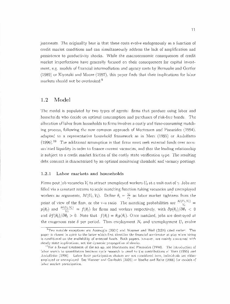
justments. The originality here is that these costs evolve endogenously as a function of
credit market conditions and can simultaneously address the lack of amplification and
persistence to productivity shocks. While the macroeconomic consequences of credit
market imperfections have generally focused on their consequences for capital invest
ment, e.g. models of financia! intermediation and agency costs by Bernanke and Gertler
(1989) or Kiyotaki and Moore (1997), this paper finds that their implications for labor
markets should not be over100ked 9
1.2 Model
The model is populated by two types of agents: firms that produce using labor and
households who decide on optimal consumption and purchases of risk-free bonds. The
allocation of labor from households to firms involves a costly and time-consurning match
ing process, following the now common approach of Mortensen and Pissarides (1994),
adapted to a representative household framework as in Tvlerz (1995) or Andolfatto
(1996).10 The additionaJ assumption is that firms must seek external funds over accu
mulated liquidity in order to finance current vacancies, and that the lending relationship
is subject to a credit market friction of the costly state verification type. The resulting
debt contract is characterized by an optimal monitoring threshold and vacancy postings.
1.2.1 Labor markets and households
Firms post job vacancies vt to attract unemployed workers Ut at a unit cost of Î'. Jobs are
filled via a constant returns to scale l1latching function taking vacancies and unemployed
workers as arguments, M(Ut , Vt). Define et = ~ as labor market tightness from the
point of view of the Finn, or the v-u ratio The matching probabilities are fl.J(I~,vtl =
p(el ) and M(~,',.V,) = j(et) for firms and workers respectively, with fJp(etllôet < 0
and ôj(etllfJet > O. Note tbat j(e t ) = etp(et ). Once matched, jobs are destroyed at
the exogenous rate c5 per period. Thus employment Nt and unemployment Ut evolve
9Two notable exceptions are Acemoglu (2001) and Wasmer and \Veil (2004) cited carlier. This paper is dosest. in spirit to the latter which hrsl identifies the financial accelerator at play when hiring is condit:ional on the availability of external funcls. Both papers, however, are mainly concerned \Vith steady state implications, not. the dynamic propagation of shocks.
IOFor a formai treatment. of the set-up, see i\Jortensen and Pissarides (1994). The int.roduction of labor search 1,0 quantitative business cycle research is owed to the contributions 01 1\ 1en, (1995) and AncloJfatto (1996). Labor force participation choices are not considered here, individuals are either employcd or unemployed. See Wasmer ancl Caribaldi (2005) or Haefke and Reite (2006) for models of labor market participation.
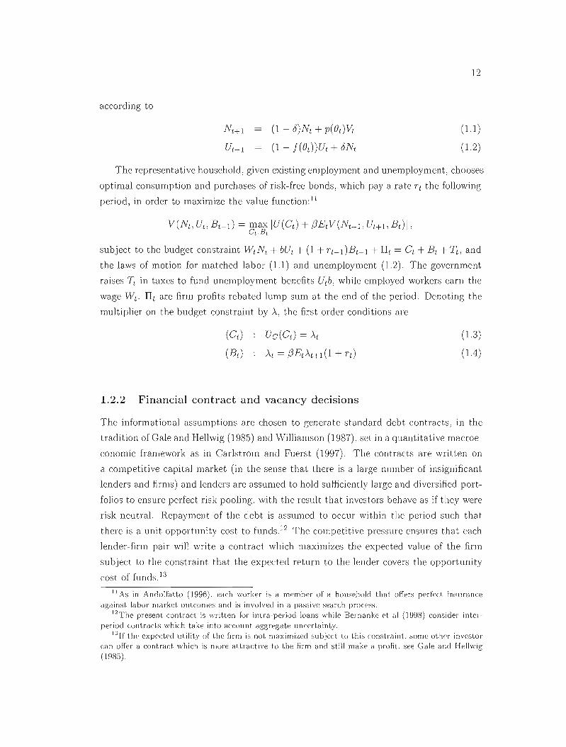
12
according to
NH1 = (1 - o)Nt + p(Bt)Vt (1.1 )
UH1 (1 - f(B,J)Ut + oNt (1.2)
The representative household, given existing employment and unemployment, chooses
optimal consumption and purchases of risk-free bonds, which paya rate Tt the following
period, in order to maximize the value function: 11
V(Nt ,Ut, Bt- 1 ) = ~~; [U(Ct) + {JEt V (Nt+1 , UH1 , Bd],
subject to the budget constraint WtNt + bUt + (1 + Tt-l)Bt- 1 + TI t = Ct + Bt + Tt, and
the laws of motion for matched la bor (1.1) and unemployment (1. 2) The government
raises Tt in taxes to fund unemployment benefits Utb, while employed workers earn the
wage Wt . TI t are finn profits rebated lump sum at the end of the period. Denoting the
multiplier on the budget constraint by À, the first order conditions are
Uc(Ct ) = Àt (1.3)
Àt = {JEtÀt+ l (1 + Tt) (1.4 )
1.2.2 Financial contract and vacancy decisions
The informational assumptions are chosen to generate standard debt con tracts, 111 the
tradition of Gale and Helhvig (1985) and 'vVilliamson (1987), set in a quantitative macroe
conomic framework as in Car!strom and Fuerst (1997). The contracts are written on
a competitive capital market (in the sense that there is a large number of insignificant
lenders and hrms) and lenders are assumed to hold sufficiently large and diversihed port
folios to ensure perfect risk pooling, with the result that investors behave as if they were
risk neutra! Repayment of the debt is assumed to occm within the period such that
there is a unit opportunity cost to funds 12 The competitive pressure ensures that each
lender-firm pair will write a contract which maximizes the expected value of the finn
subject to the constraint that the expected return to the lender covers the opportunity
cost of funds. 13
J J As in Andolfatto (1996), each worker is a member of a househoJd thal offers perfect insurance against labor market outcomes and is involved in a passive search process.
12The present contra,ct is written for intra-period loans while Bernankc et al (1998) consider interperiod c:ontracts which take into acc:ount aggregate uncertainty.
13If the expected utility of the finn is not maximized sllbject to this c:onstraiul. sorne other investor Uln oHer a contrac:t which is more attractive to the firm and still make a profit. see Gale and Hellwig (1985).

13
Define firm period net revenues as x (X - W) N, where X is the aggregate level of
technology, W is the wage rate and x is a random variable, i.i.d. across firms and time,
with positive support, cdf H(x), pdf h(x) and E(x) = 1. 14 The crucial assumption is
that agents have asymmetric information over the realization of the random variable x.
This state can only be observed by lenders at sorne cost proportional to realized net
revenues, 0 < ~ < 1.
The timing of events in each period is as follows. Assume that vacancy costs l'V
must be paid before production occurs. Ail agents observe the aggregate state X and,
given initial assets A, firms borrow (l'V - A) from financial markets to pay for period
vacancy postings15 Lenders and borrowers agree on a contract that specifies a cutoff
productivity x such that if x> x, the borrower pays x (X - W) N and keeps the equity
(x - x) (X - W) N. If x < x, the borrower receives nothing and the lender claims the
residual net of monitoring costs.
Define the expected gross share of returns going to the lender as
f(x) = r xdH(x) + Ccc xdH(x)Jo Jx
noting that ri (x) 1 - H(x) > 0 and rl/(x) = -h(x) < 0, and expected monitoring
costs as
I-LG(X) = ~ lX xdH(x)
\Vith ~GI(X) = ~Xh(X).16 It is easy to see that the expected gross share to the lender
will always be positive.17 Given this set of definitions we can conveniently express
the lender's participation constraint as [f(x) - I-LG(X)] (X - W) N = (l'V - A): which
states that the returns net of monitoring costs must equa.l the value of the loan.
Given the assumptions on the functional forms: notably constant returns to scale in
production and a linear monitoring technology: onl)' the evoJution of aggregate assets
is needed to know the cost faced by firms on credit markets and ail firms will choose
14 Alternatively the firm's period net revenue could be expressed as (xX -IV)N with x c1rawn from a positive support with lower bound W. Either formulation guarantees a positive payoff function ensuring that the problem is weil definecl. This is similar to the approach in Carlstrom and Fuerst (2000) \Vhich consists of assuming that firms sell their product at a time varying mark-up over costs.
15Bank loan models, as in Christiano. Eichenbaum and Evans (2005) for example. assume thot ail current costs, in their case the \Vage bill, must be Ilnanced by bank loans. The assumption of a fraction of vacanc)' cost needing external financing js consistent \Vith evidence on firm financing. such as Devereux and Schiantmelli (J989) and sufficient to generate the results in this paper.
lGThe expected share ofreturnsgoing to the borrower under thecontracl is T(x) = frOC (x - x) dJl(x). Note that ['(x) + Y(x) = 1.
J7To do so. take the limits lirnJ_o r(x) = I; xdJ1(x) = O. lilllT-x ['(x) = IoC<: ;rdJ-J(x) = .1 > 0 and recall that f(x) is strictly increasing and concave in x.

14
the same ratio of vacancies to assets (see Carlstrom and Fuerst, 1997). These evolve
according to AH1 = ç [1 - [(Xt)] (X t - Wd Nt, where the parameter a< ç < 1 ensures
self-financing does not occur I8 Rearranging as
focuses on the premium associated with external funds, tLG(x~~~~~~tlNt, which for any
J.t > a is strictly positive.
We can now write the optimal incentive compatible contracting problem with non
stochastic monitoring and repayment within the period. Vacancy postings and the
threshold x are chosen to maximize the expected gross return to the fifln subject to the
lender's participation constraint
and the laws of motion for employinent (1.1) and aggregate assets (1.5), where firms use
the stochastic discount factor ,6Et À~~J .
1.2.3 Job creation under credit constraints
Denoting the multiplier on the lender's participation constraint by cP, the optimality
condition for vacancy postings describes a job creation condition
equating the average cost of a vacancy: ;(~,t), to the expected marginal value of an
additional employed worker ,6Et"\~'1 Jn (NH 1· AL+d·
In order to derive the marginal value of a worker to the finll, Jn(NL, Ar), differentiate
the firm's value function \Vith respect to N:
J6The assumption of sorne depletion in the stock or assets is needed to rule out eveMual selr-financing. CarJstrom and F\lerst (1997) assllme that consumers and entrepreneurs have difTerent time discount ractors, while Bernanke, Gertler and Gi1christ (1999) assume that a haclion or the entrepreneurial popuJation exits every period consuming their assets on the \Vay out. It is assumecl here that firms retain a rraction or their earnings to\Vard next period's assets while rebating the remaining to households as profits.

15
The first term corresponds to the net return on an employee accruing to the fifln under
the debt contract. The second term captures the value an additional worker brings to
the firm by relaxing the financing constraint in terms of an increased ability to reimburse
the loan. The final term captures the value of the continued relationship. For the sake
of simplifying the notation, cali D(Xt) == 1 - r(Xt) + cPt [r(Xt) - p,G(Xt)]. Combining
the marginal value of a worker with the optimality condition for vacancies, and making
use of the household bond Euler eqllation (1.4), yields the intertemporal condition for
vacancy postings
"(cPt 1 [(_) ( ) ) ,,(cPt+ 1 ] -(B) = --Et D Xt+1 X t+1 - Wt+ 1 + (1 - 6 (B ) (1.6)P t 1 + Tt P t+1
At this stage it is useful to show how this setting with credit frictions compares with
a standard labor search model. Consider first the credit constraint multiplier cPt on the
cost side of the job creation condition. From the first order condition for the clltoff
productivity, the multiplier may be expressed as
ri (Xt) (1. 7)
cPt = [r'(xd - p,G'(Xt)]
ln the absence of monitoring costs the threshold x tends to the lower bOllnd of its support.
It is straightforward to show that ocPt!OXt > 0, and that in the Iimit limxt ...... o cPt = 1.
That is, for any positive monitoring cost, the presence of credit frictions drives up the
average cost of vacancy postings to Ptt) ,as opposed to P(~L)' where cPt can be interpreted
as the shadow cost of external over internaI funds.
Second, one can show that limxl->o D(xd = 1 , such that in the absence of monitoring
costs the first order condition (1.6) collapses to the standard job creation condition in a
stochastic discrete time setting:
"( 1 [ - l' ]-(B) = -1-.Et X t+1 - Wt+ 1 + (1 - 0) (B ) (1.8)P l, +Tt P Hl
The received argument for the lack of amplification of plOductivity shocks is easily
understood by this job creation condi tion equating the average cost of a vacancy to
the expected benefit of a ne\V job (see ShimeL 2005. Hall, 2005). A sudden rise in
productivity, increasing the profits to the fifln of a job. increases the incentive to post
vacancies. The same rise in productivity, however, leads to a rise in the wage reducing
the profits to firms For most applications of the Nash bargaining solution. the wage is
highly elastic to productivity such that the profits from a job for the finn are relatively
inelastic to productivity shocks and, as a consequence: so are vaC811CY postings. There
is. however, a second, overlooked. c1ampening lI1echanism built into the job creation

16
condition. The same event leading to a rise in the job finding hazard for workers, and
their abili ty to negotiate higher wages, also corresponds to an increase in the congestion
facing firms. ln other words, each job vacancy faces a decreasing probability p( Bt ) of
being filled in a given unit of time. This increase in the average cost of hiring a worker
further restricts finn entry, limiting the propagation of productivity shocks.
The first response ta this issue has been ta induce greater wage rigidity by either
changing the structure of the model, i.e. settling on different wage determina tion mech
anisms (HalL 2003, Gertler and Trigari, 2009, Menzio, 2006), or following a calibration
strategy resulting in a wage less elastic ta productivity (Hagedorn and Manovskii, 2008).
Here, credit frictions have the potential ta amphfy pl'oductivity shocks in manner that
is fundamentally different, operating through the cast side of the job creation condition.
Recall that in the presence of credit frictions the average cost to filling a vacancy is p(t:) , whereas in the standard model it is (~). The multiplier on the lencier's participation
p 1
constraint, rPt, which, as a measure of the shadow cast of external over internai funding,
indicates how binding credit constraints are, in effect drives a time-varying wedge on
the cast side relative ta the frictionless modeL If these constraints are counter-cyclical,
or rPt decreases during an economic upturn, there is a downward push on the average
cast of vacancies that increases the incentive for firms to post vacancies]9
1.2.4 Workers and wages
The model is fully described once the rule for wages is determined. ln arder to define the
values of a job (Vn) and unemployment (Vu) ta a worker, ciifferentiate the householci's
value function \Vi th respect ta N and U:
Vn(Nt , Ut, Bt- J ) ÀtWt + (3EL [(1 - 6)Vn (NHJ , UL+1 , Bd + 6Y;I(NL+1 , UL+1 , Bt )]
Vu(Nt , UL, BL- J ) = ÀLb + (3Et [(1 - f(Bd)Vtl(NH1 . UH1 , Bd + f(BdVn(NHj · UL+1: Bd]
The current value of a job corresponds to the wage measurecl in utils and the discounted
expected values of next period's state, which with probability (1 - 6) remains employ
ment. The value of unemployment is derived froll! the value of non-market activities,
Àtb. and the discounted expected value of next period's state. wllich \Vith probability
f(Bd is 8mployment.
191n this formulation t.hese constraints are counter-cyclical as the profîtabi]ity on the investmenl project, here the nel return from Jabor. rises more quickly than the leverage taken on by borrowers during an expansion. For a detailed analysis of the condilions under which credit market. frictions crea le a fînancial accelerator which destabilizes the economy. see Bouse (2006).

17
Splitting the surplus of a worker-firm match, defined as S(t) = Jn(t) + Vn(t);tVu(t) ,
under a generalization of Nash bargaining, as in Pissarides (2000), yields the wage rule20
(1.9)
where Wt = 1/ [1 + 1](D(xd - 1)]. As \Vith the job creation condition, when monitoring
costs tend to 0 the wage rule (1.9) collapses to
(1.10)
This is simply the usual the wage rule without credit frictions and leads to the following
proposition
Proposition 1 - The canonical Mortensen-Pissarides search and matching model of
equilibrium unemployment is a special case of the present model with frictional credit
markets when the cost of monitoring tends to zero.
While we will discuss in the next section the steady state and quantitative impli
cations for labor-market dynamics, one important aspect of the modified wage rule is
worth stressing here. A principal force in the cyclical properties of the wage rule is the
tenn 'YrPtBt which, along with the value of non-market activities, captures the relative
bargaining positions of workers and firms. During an upturn, market tightness rises
making it more costly for firms to pull out of the wage negotiations to search for another
worker (recall that a rise in B implies a drop in the probability of meeting a worker p(B)).
In the presence of credit market frictions, the cost of a vacancy ,rPt actually decreases
during good times as conditions on credit markets improve. The strengthened bargain
ing position of firms Iimits somewhat the upward pressure on \vages stemming from the
rise in market tightness. The end result is to induce some degree of wage rigiclity \vhich
will contribute to amplifying productivity shoc1<s in the manner outlined above 2!
1.2.5 Closing the model
From the household's budget constraint it is straightforward to derive 8n aggregate
resource constraint
20Wages are negotiated at the beginning or the pC'riorl once the aggregate state is observed but before the Ilrm draws an idiosyncratic productivity. Tlle wage is not a function of the idiosyncratic productivitv. lest it reveal the firm's productivity draw to creditors. but will refJect the terms faced by the firm on credit markets. lt is assumed that \l'ages cannot be renegotiated ex-post. Details on the derivation of the \l'age me presented in the appendix.
21 As n note, both ",'/ and O(XI) are relativel)' inelnstic to productivity and will contribute only mnrginallv to fluctuations in wages.

18
where Yi = XtNt, fLG(Xt) are resources consumed in monitoring and "(Vi are vacancy
costs.
The equilibrium of the model is then characterized by equations (1.3) and (1.4)
from household optimization, a job creation condition (1.6), optimality condition for
the threshold Xt in (1.7), the clefinition of market tightness, the lender's participation
constraint, a wage rule (1.9), the aggregate resource constraint and Jaws of motion for
asset accumulation, aggregate employment and unemployment.
1.3 Propagation properties of financial and labor market
frictions
Before discussing some of the steady state labor market implications of credit market
frictions in this setting, the assumptions on functional fonns and calibration are pre
sented in detail. The model is then solved by computing the unique rational expectations
solution for a log-linearization around the deterministic steady state, and the dynamics
are evaluated with a series of unconditional second moments and impulse response func
tions. The performance of the model is assessed by simulating a standard labor search
model as a basis for comparison and performing a series a sensitivity analysis to key
parameters and aspects of the mode!.
1.3.1 Functional forms and calibration
Following much of the real business cycle literature, aggregate technology is assunled
stationary and to evolve according to
log X t = Px log X 1- 1 + E{:
with E{ '" (0, (J~) and 0 < Px < 1. Staying within this literature, the relevant parame
ters are chosen as Px = 0.975 and (Jx = 0.0072 (e.g., King and RebeJo, 1999).
For household preferences, period utility is defined as u( C) = log C. The idiosyn
cratic shock x is assumed to follow a log-normal distribution with mean E(:r:) = 1; i.e. 20
log(:r:) '" N( - lo~(:r); (J~g(x))' Finally following much of the 13bor search literature, the
matching technology is a Cobb-Douglas M(U, Y) = XU<,yl-<" with 0 < E< 1 and X> O.
The model is calibrated to quarterly data. The discount factor f3 = 0.992 is set so
as to match an average anllual real yield on a risk less 3-month treasury bill of 3.3%.
For parameters pertaining to financi<ll factors, the quarter!y default rate is set to 1%,

19
in the range of values reported in both Carlstrom and Fuerst (1997) and Bernanke et
al. (1999), and implies a standard deviation of the idiosyncratic productivity ax of
0.12. The resource cost of monitoring is set to J-L = 0.0375 so as to match a 3% steady
state premium on external funds, which corresponds to the mid range of the spread
between AAA and BAA commercial paper and a 3-month treasury bill over the period
1977-2004.22 This resource cost of monitoring is much lower than in Carlstrom and
Fuerst (1997) or Bernanke et al. (1999) in which it is set at 0.25 and 0.12, respectively.
Evidence in Devereux and Schiantarelli (1989) suggests that firms fund over two thirds
of their current expenses with internaI funds, which is used to pin down the value of
the parameter ç. However, it is important to stress that in this model the fraction of
current costs funded externally is in fact Î.\)~~N' which for any calibration is a very
small fraction (around 1 to 2%)23 Other investigations, such as Christiano et al (2005)
assume that ail current costs, in their case the entire wage bill. must be financed through
bank loans. The sensitivity of the results to the calibration of the credit market will be
examined below.
Several authors have argued that the targeted steady state rate of uJ1elllployment
should include more than the rate of workers counted as unemployed as the model does
not account for non-participation. Krause and Lubik (2007), for example, choose an
unemployment rate of 12%, above the average rate observed for the United States. The
benchmark calibration, however, will target a 7% unemployment rate as in Gertler and
Trigari (2009). The cost of job vacancies is set to Î' = 0.125, in the range of values
suggested by the studies of Baron (1997) and Baron (1985), as cited in Ramey (2008).
The elasticity in the labor matching function, E, is set to 0.6, which lies below the value
of 0.72 used in Shimer (2005) but weil within the range of values identified by Petrongolo
and Pissarides (2001) in their SUl·vey of the ma tching function. The bargaining weight
of the household in the wage negotiation. IJ, is set to 0.5. This mid-point is <.:hosen to
strike a balance between the extremes advocated in Hagedorn and lVlanovskii (2008) and
Shimer (2005)24 FinaJly. the quarterly rate of job separation is set to 6%, corresponding
to the evidence presented in Davis, Faberman and Haltiwanger (2006), and the value of
X is chosen to obtain a job filling rate of 0.6
The benchmark calibration results a replacement rate b/w of 0.81. It is weil known
22The yields are for I\loody's seasoned AAA and BAA corporate bonds. 23ln relaLed evidence, Buera and Shin (2008) sugg<'st that firms fund over 50% of their capiLal
expendiLure with exLernal funds. 24The former adopL an extremely low vDiue of L1lP bargDining pDrameter in orcier to generate D wage
with a low elasLiciLy to prodllctivity. The latter seLs Lhe bargaining weight equal to the weight on lInemployment in the IllDtching function DS lInder the ·JJosios (1990) rule' in order to ensure constrained efficiency of the decentralized solution.

20
that the properties of labor search models change dramatically as this ratio tends to
unity, and setting a high value as advocated by Hagedorn and l\!lanovskii (2008) has
the unappealing implication that workers gain little utility from accepting a job (see
Mortensen and Nagypal, 2007).25 While there is no definitive value for the replacement
rate, the present calibration tries to stay clear of such issues by straying closer to the
value used in Elsby and Michaels (2008).
1.3.2 Steady state implications
Proposition 2 - There exists a unique steady state equilibrium in which the mte of un
employment is strictly increasing in the resource cast of monitoring] p.
Proof. The job creation condition in the presence of credit constraints can be used
ta pxprpss the wagp FI.s a dpfTP8.sing functian of markPt tightnpss
1 ) 4nw=l- ( ~-(1-0) D(x)p(8)
where aggregate productivity has been normalized to 1. Relative the to case with perfect
credit markets, the additional cost induced by the necessity of external funds implies a
steeper curve by the factor Dfx) > 126 Figure 1.1 plots in (8,w) space the job creation
curve for the model with (solid line) and without (dashed line) credit frictions. The
wage rule in the presence of credit frictions, w = ryw(D(x) + t<p8) + (1 - ry)wb, has a
slope wryt1J greater than in the absence of credit market friction by the factor w1J > 1
capturing the greater opportunity cost of a match to the firm that workers can exploit
and, conditional on w (ryD(x) + (1 - 7])b) < l, the intersection of the wage rule and job
creation condition is unique.
Combined, the two labor market equilibrium conditions, the job creation and wage
rule, pin down equilibrium market tightness 8 as
25The strategy employed here is to pin down the vulue of non-murket ucl.ivil.y such us to mutch an observed unemployment rate. This approach avoids some of the controversy surrouuding the value of this parameter. Hagedorn and l\lanovskii (2008) reconcile the standard search mode] with key labor market statistics by employing an elevated value of the replacement rate of 0.96. Rotemberg (2006) chooses a value of 0.9, while Elsby and 1\1 icllélels (2008) set the rate at a lower 0.86.
26 o· . l' .. - d l' 0 lO(Y) lS strict y IOcreaslng ln x an J01:ë-O ~)(:T) = .

21
1.02!
092
o9~agerule_------------
088- _, ....... ~
086~ __ - - -
0.5 1.5 e' 2.5
Figure 1.1: Steady state la bol' market equilibrium
which in the absence of credit friction is given by
where e- denotes equilibrium market tightness in the frictionless case. e < e* fol1ows
from the fact that <P > ] and w~x) > 1 for any strictly positive value of the monitoring
cost f-l. To see the effect of an increase in f-l on market tightness, consider first tha t
~~ > 0, or that the measure of credit constraint is increasing in monitoring costs. Since à_O_
it is also the case that wàn~I) > 0, an increase in monitoring costs leads to a decrease in
equilibrium labor market tightness which, through the Beveridge relationship, implies a
greater steady state rate of unemployrnent.27 This insight is similar to that in Acemoglu
(2001) and Wasmer and Weil (2004) in that credit frictions restrict firl1l entry on labor
markets. Combinee! with a greater wage for every level of market tightness, credit
frictions unambiguously lead ·to greater equilibriul1l unemployment.
1.3.3 Dynamic results
Several authors, as mentioned earlier, have noted the failure of the lVlortensen-Pissarides
framework to generate sufficient internaI propagation of exogenous shocks to match key
labor market statistics. Table 1.1 reports the Hodricl<-Prescott filtered standard devi
ations relative to aggregate output of variables centra! to the labol' market.. along with
their conternporaneous correlation \Vith the cyclical cornponent of aggregate output.. The
27 The elIect on the equilibrium wage is ambiguous as higher recruiting Cùsts both lowers job olIer:; and affects the threat point in wage barg<1ining to the advantage or workcrs.
22
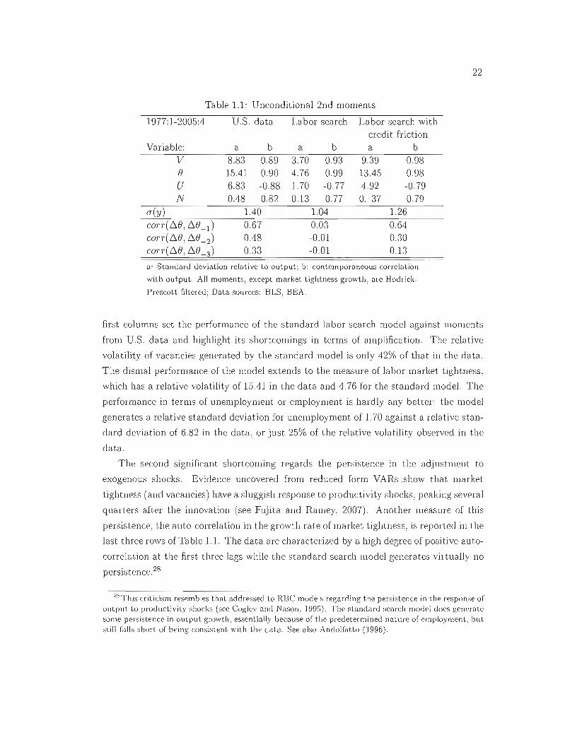
Table 1.1: Unconditional 2nd moments
1977:1-2005:4 U.S. data Labor search Labor search with credit friction
Variable: a b a b a b V 8.83 0.89 3.70 0.93 9.39 0.98 8 15.41 0.90 4.76 0.99 13.45 0.98 U 6.83 -0.88 1.70 -0.77 4.92 -0.79 N 0.48 0.82 0.13 0.77 O. 37 0.79
a(y) 1.40 1.04 1.26
corr( 6.8, 6.8-1) 0.67 0.03 0.64 corr(6.8,6.8_ 2 ) 0.48 -0.01 030 CO'rr( 6.8: 6.8_ 3) 0.33 -0.01 0.13
a: Standard deviation relative to output; b: contemporaneous correlation
with output. Ali moments, except market tightness growth, are Hoclrick
Prescott filtered; Data sources: BLS, BEA.
first columns set the performance of the standard labor search model against moments
from U.S. data and highlight its shortcomings in terms of amplification. The relative
volatility of vacancies generated by the standard model is only 42% of that in the data.
The dismal performance of the model extends to the measure of labor market tightness,
which has a relative volatility of 15.41 in the data and 4.76 for the standard model. The
performance in terms of unemployment or employment is hardly any better: the model
generates a relative standard deviation for unemployment of 1.70 against a relative stan
dard deviation of 6.82 in the data, or just 25% of the relative voJatility observed in the
data.
The second significant shortcoming regards the persistence in the adjustment to
exogenous shocks. Evidence uncovered from reduced form VARs .show that market
tightness (and vacancies) have a sIuggish response to prod uctivi ty shocks, peaking several
qualters aI'ter the innovation (see Fujita and Ramey, 2007). Another measure of this
persistence, the auto-correlation in the growth rate of market tightness, is reported in the
last three rOWs of Ta ble 1.1. The data are characterized by a high degree of posi tive au to
correlation at the first three lags while the standard search model generates virtually no
persistence.28
2bThis criticism resembles that addressed to Rue models regarding the persistence in the response of output to productivity shocks (see Cogley and Nason. 1995). The standard search model does generate some persistence in output growth, essentially because of the predetermined nature of employment, but still falls short of being consistent with the data. See also Andolfatlo (1996).

23
1.3.3.1 Vacancies and labor market tightness
We begin by examining, in Figure 1.2, the responses of vacancies and market tightness
to a positive productivity shock in the standard (dashed line) and proposed (solid line)
models. The introduction of credit frictions yields two improvements: first, the response
is greatly amplified; second, the response is persistent, or the adjustrnent to the ex
ogenous innovation is 'sluggish.' The unconditional second moments for the proposed
model, presented in the last columns of Table 1.1, show that relative volatility of va
cancies is large, at 9.39, and close to the value of 8.82 found in the data. The labor
market tightness generated is also remarkably close to its empirical counterpart with a
measure of relative volatility of 13.45, compared to 15.41 in the data. ln term of per
sistence, vacancies, and market tightness, peak several quarters aEter the shock. More
precisely, the model generates elevated positive autocorrelations in the growth rate of
market tightness that are very close to the data at the first two lags, although decaying
too rapidly at the third (see the last three rows of Table 1.1).
The large propagation potential of financial frictions results in a standard deviation of
aggregate unemployment of 4.92, whereas the volatility of unemployment in the standard
model is only 1.70 against 6.83 in the data. The standard deviation of aggregate output
in the model with credit frictions, at 1.26; is closer to the value of 1.40 in the data. A
standard labor search mode! generates a volatility of aggregate output barely beyond the
impulse provided by the exogenous process with a standard deviatioll of 1.04. Figure 1.4,
which plots the responses of output and unemployment to a positive productivity shocle
illustrates the full impact of this financial accelerator on aggregate activity. Output
continues to expand severa! quarters aEter the standard model has reached its peak and
the strong flows of hiring lead to a deep drop in the unemployment rate.
Understanding the present results lies in the dynamics of the cost and wage channels
of propagation outlined earlier. As both depend on the evolution of the shadow cost of
external funds cP; the first panel of Figure 1.3 plots the response of this measure of credit
constraints folJo\oving the same expallsionary shock to productivity. While the constraillt
is relaxed on impact, the slo\',; accumulation of assets pushes the constraint to its !owest
several periods aEter the shock. The effect on the job creation condition through the cost
of vacancies is strongesL therefore. several periods after the shock. as seen in Figure 1.2.

24
Vacancies Marl<ellighlness e 20" ~ '-Searchwilhcredithiclion
! 18 ~ / Standard labor search l'li 16L.
il'" ~ ~'2" ___.. g 10 ~ _________
~ 8
~ 6<Il U 4
------- "" 0--------------- 0---------- -- o 10 15 20 25 30 35 40 o 10 15 2Q 25 35 40
Penods Penods
Figure 1.2: IRFs to a positive productivity shock, vacancies and market tightness
'Nage
-CIO("r-cx<J9~fIOIr.l" 1I - - - Sr:vlGlill,d labof so&'ch
-: , .. ••• 1 " . '0 2O 25 30 OS '0 '0 2O ;. 30 OS '0
" PcrlOOs " Pc!',ods
Figure 1.3: IRFs to a positive productivity shock, shadow cost of external funds and wage
The wage channel is illustrated in the second panel of Figure 13. Following an
innovation to productivity, wages do not respond initially as strongly as in the standard
model, and increase progressively for several quarters. This rigidity contributes to the
elasticity of the initial response of market tightness and vacancies to a productivity shock,
which is greater in the model with credit frictions (again. see the first panel of Figure
1.2). The ensuing ri se in the wage, as market tighlness continues to rise faster than
4> decreases, counters some of the relaxing of the financing c:onstraint for job creation.
HoweveL the continued rise in vacancies is testill10ny to the fact that the cost channel
is largely dominant The joint effect of these channels cxplains why the peak in market
tightness is reached 6 quarters after the initial shock.

25
Unemploymenl OUlpUI o , 1.0
CrediT - exogenous 0 - - ~ Standard Labor searCh
0.8
0.6
-80o--~'----:':,0-----":-"----=''::-0--:!2S 3~ :;) do O.40~-"---'"="O --,"=",----=20'::------=2~5----=:JO'::------=J5'::--~'" Periods PO!!lf>dS
Figure 1.4: IRFs to a positive productivity shock, Itnemployment and output
1.3.3.2 The shadow cost of externaI funds and robustness to the
calibration of the credit market
The strength of these results relies on the degree of responsivr-mess of the shadow cost of
external funds, cP, to changes in aggregate productivity. At the height of the response
to a positive innovation, this measure of financing constraints can drop by up to 15%
relative to is steady state value, representing a high degree of volatility. While their
is no empirical counterpart to verify directly the realism of such large changes, it is
possible to compute the volatility implied on the premiuJI1 on external funds, expressed
as J1G(Xt)~Xt~Wt)Nt. and how it compares with the data. For example. the spread on AAA ""Y t- t . .
and BAA bonds have, respectively, standard deviations relative to output of 0.66 and
0.70, and contemporaneous correlations with output of -0.58 and -0.67. The benchrnark
calibration implies a preOlium that is slightly more volatile than for the highest Cjuality
commercial paper, with a relative volatility of 0.93 and a contemporaneous correlation
with output of -0.98. The mode!' however. speaks more to the relation between the state
of credit markets and fluctuations in the rilte of unernployment. Along this dimension,
the contell1poraneous correlation of unemployment with the premium for the benchmark
calibration is 0.82. This lies just above the correlations for the spreads in the data with
unemployment. which is 0.62 on AAA bonds and 0.72 for BAA bonds.
To further ascertain the robustness of the results, the first columns of Table 1.2
present the effects of calibrating on either a 1% or a 4% prellliulll by changing the
resource cost of monitoring compared to the benchmark. A Jower premium on external
funds implies il reduced propagation of productivity shocks, the volatility of the v-u
ratio dropping to 9.53 and the relative voJatility of unelllployment to 3.48. The inverse
is observed when the premiuIll on externa! fil18I1Ce is raised to 4o/c" the relative standard

26
Table 1.2: Robustness to credit market parameterization
Benchmark Premium
1% 4% 50% 90%
a b a b a b a b a b
U 4.92 -0.79 3.48 -0.75 5.50 -081 2.75 -0.69 6.08 -0.86
V 9.39 0.98 6.74 0.99 10.49 0.99 5.28 0.99 11.89 0.96
B 13.45 0.98 9.53 0.98 15.03 0.98 7.5 0.95 16.68 0.99
CJ(y) 1.26 1.14 1.32 1.08 1.44
corr(6B, 6B -1) 0.64 0.49 0.66 0.42 0.52
corr(6B, 6B -2) 0.30 0.25 0.30 0.29 0.17
corr(6B, 6B -3) 0.13 0.12 0.12 0.19 0.05
a: Standard deviation relative to output; b: conternporaneous correlation with output.
Ail moments are Hodrick-Prescott filtered; Data sources: BLS, BEA.
deviation of e rising to 15.03. \Vith respect to the measure of persistence: the change
in the premium affects mainly the auto-correlation at the first lag: a higher premium
generating a greater coefficient. This occurs through a greater short l'Un elasticity of the
shadow cost of external funds to changes in productivity.
Next, the implications of changing the fraction of vacanc)' costs requiring external
funds is examined in the last columns of Table 1.2. While this changes little the steady
state premium on external funds: by affecting the elasticity of assets to aggregate shocks
it changes significantly the dynamics of the shadow cost of external funds. For example,
requiring 90% of vacancy cost to be funded externally increases the relative standard
deviation of the v-u ratio to 16.68 and causes the short l'un auto-correlation in the growth
rate of e to decay more rapidly. When the fraction is redllced to 50%: there is little
change to the persistence properties of the model but most of the result of amplification
disappears. Further, reducing the cost of monitoring such that the premium on externa!
funds funds tends to 0, along with reclucing the requirement on external funds below 5%
essentially reproduces the results of the standard model both in tenns of volatility and
persistence.
1.3.3.3 Sensitivity to the calibration of the labor market and volatility of
wages
This section first examines the sensitivity of the main results to changes in the calibration
of labor market specific parameters. \Vith results presentecl in Table 1.3. we look at the
impact of variations in the unit cost of vacanc:ies. the elasticity of the matching function
\Vith respect to unemployment and to c1ifferent steady state rates of lInemplo)'ment.

27
The dynamic properties of ail labor search models are very sensitive to the value of
unit search costs "f. When targeting a specifie rate of lInemployment, is implies quite
different replacement ratios. For example, increasing its value from 0.125 to 0.25 reduces
the replacement ratio to 63%. As a result the standard deviation of output drops from
1.26 to 1.09 while the relative volatility of labor market tightness declines to 7.80 from
13.45. The appropriate comparison however, in terms of evaluating the robustness of
the results stemming from the inclusion of credit market frictions, is with those from
the standard search model with Î' = 0.25. Under such a scenario, the relative standard
deviation of the v-u ratio generated is only 2.50, leading to the conclusion that the
result of amplification is robust to variations in the unit cost of job vacancies. 1f the
unit cost is reduced to 0.075, the standard deviation of market tightness increases to
18.62 in the model with credit friction and to 7.40 in the standard mode!. With regards
to persistence, on the other hand, variations in the unit cost of vacancies have very little
effect on the results presented for the benchmark calibration.
The elasticity of the matching function \Vith respect to unemployment governs the
manner in which movements in labor market tightness translate into changes in the
hazard ra tes faced by workers and firms. A red uction in the elastici ty wi th respect to
unemployment, which increases the elasticity of the job finding rate to variations in mar
ket tightness, greatly increases the response of aggregate unemployment and output to
exogenous innovations. For example, decreasing ( from 0.6 to 0.5 increases the standard
deviation of output to 1.36 and the relative volatility of unemployment to 5.91. On
the other hand, the incentives to post vacancies becomes less sensitive to the business
cycle and the relative volatilities of both job vacancies and the v-u ratio decrease. The
stronger movements in the rate of unemployment however, a stock variable in the mode!.
tends to increase the persistence in the growth rate of market tightness at the first three
lags, and rnost n'otably at the first. Increasing the value of the parameter é to 075 has
the inverse effects.
Finally. raising the target steady-state rate of lInemployment, \Vhile increasing the
volatility of aggregate output, has only a minor down,vard impact on the relative volatil
ities of vacancies, unemployment ancl the v-u ratio, and very little impact on the measure
of persistence. The converse is true for a reduction in the target steady state rate of
unemployment. Overall. the moclel behaves in its weli-kno\Vn directions (see Yashiv.
2006), and the main propagation mechanisl1l outlincd in the mocle] is not altered by the
calibration of the labor market.
The current model rcsulted in a certain c1egree of wage rigidity contributing ampli
fication beyond tha t origina ting from the cost channel ou tli ned above. The cali bration

28
Table 1.3: Robustness to labor market parameterization
u 0.075 0.25 0.5 0.75 006 0.10
a. b a b a b a b a b a b
U 6.81 -0.86 2.85 -0.70 5.91 -0.81 3.29 -0.74 5.13 -0.78 433 -0.81
V 12.99 0.98 545 0.99 8.10 0.97 1166 099 9.27 0.99 9.7 0.96
() 1862 0.99 7.80 0.95 12.90 0.98 14.40 0.98 13.64 0.97 1294 0.99
ury) 1.51 1.09 1.36 1.13 1.21 1.39
corr(DJJ, (:;()- J) 0.64 0.63 0.71 0.51 0.65 058
corr({:;(). (:;1)-2) 0.30 0.30 0.34 0.24 0.30 0.29
corr({:;(). (:;1)-3) 0.13 0.13 015 0.10 0.12 0.14
a: Standard deviation relative to output; b: contemporaneous correlation \Vit.h output..
strategy employed by Hagedorn and IVlanovskii (2008), which they anchor on cyclical
properties of an aggregate wage series, results in a standard deviation relative to output
in the order of 0.20. Both Pissarides (2008) and Hael1<e et al. (2008), however, argue
that the empirically relevant wage is that of new matches, or hires, which is character
ized by near proportionality with productivity.29 To situate in this context the degree
of rigidity induced by the credit friction for the benchmark calibration, consider that
it results in a standard deviation of wages of 0.57 whereas the standard labor search
model generates a standard deviation of 0.86.30 Therefore, it can be argued that the
wage rigidity stemming from the interaction of laboT market tightness and the shadow
cost of external funds does not generate a high degree of wage rigidi ty, certainly not to
the degree needed in Hagedorn and Manovskii (2008) to reconcile the standard model
with the volatility of labor market variables observed in the data.
1.3.3.4 Beveridge curve and cross-correlations
One concern for extensions to the standard framework is the violation of a robust empir
ical observation of a strong negative correlation between unemployment and vacancies,
or the Beveridge curve.31 Table 1.4 presents the contemporaneous cross-correlations of
key labor market variables in the data and as generated by the models. ln this respect
29For a surveys of wage time series and their properties, see Brandolini (1995) and Abraham and !laltiwanger (1995).
301'he wage in ail models is hjghly pro-cyclical in the sense of having a high degree of positive contemporaneous correlation \Vith output.
31 For instance, allowing for jobs to end endogenollsly by sorne efficient separation rllie as in i\lortensen and Pissarides (1994) Jeacls to a collnter-fadllal positive correlation between vacancies and the rate of unempioyrnent.

29
Table 1.4: Labor market cross-correlations
U.S. data
U V () J(B) YIN
U 100 -089 -0.97 -095 -0.41
V 1 0.98 0.90 0.36 () 1 0.95 0.'10
q(e) 1 0.40
YIN 1
Labor sea.rch Labor search - Credit friction
u V () J(B) YIN u V () J(B) YIN
U 1.00 -0.47 -0.73 -0.73 -0.7] 1.00 -0.74 -0.88 -0.88 -0.56
V - 1 095 0.95 0.96 - ] 0.97 0.97 o.gr)
() - - ] 1 099 - - ] 1 0.88
q(e) - - - ] 099 - - - ] 0.88
YIN - - - - ] - - - - ]
Ali moments are Hodrick-Prescott filtered; Data SO\lrces: BLS, BEA
the proposed model is again an improvement on the standnrd model with a correla
tion between unemployment and vacancies of -0.74, two third of the way between the
correlation in the data, -0.89, and the correlation generated by the standard model,
-0.47.
The data are also characterized by a very strong negative correlation between the
unemployment rate and the measure of labor market tightness, with a contemporaneous
correlation of -0.97. The standard model generates a somewhat weak correlation -0.73.
The presence of credit friction brings the correlation closer to the data at -0.88. Dy ex
tension. the proposed model also improves on the correlation between the unemploymellt
and job fin ding rates.
The proposed model is able to reduce the correlation betwcen unemployment and
labor productivity to -0.56, closer to a correlation of -0.41 in the data. This correlation
is too strong in the standard labor search model, which generates a correlation of -0.71.
This can be understood from the fact that the credit market imperfection, by ampli
fying lllovements in unemploYll1ent that peak several quarters after labor productivity,
increases the disconnect between the two time series. Both Illodels fal! short. however. of
being consistent with the correlations between labor productivity and vacancies or mar
ket tightness. These have a mild positive correlation in the data, arouncl 0.4. whereas
both models generate very high positive correlations.

30
1.4 Extension to endogenous job separation
The previous section assumed that aIl labor separations occurred at a constant, exoge
nous rate. However, endogenous job separations have been argued an important feature
of equilibrium employment models both because time varying separations are a salient
empirical observation and, by directly affecting the stock of matched job, offer an im
portant mechanism for the propagation of exogenous shocks.32 This section extends the
basic set up to allow for an endogenous labor separation margin.
1.4.1 An endogenous job separation margin
Assume that each job within a firm dra\vs an i.i.d. productivity z, where z E [0, oo( with
cdf H(z), pdf h(z) and E(z) = 1, and that this job productivity is observed by both
the worker and the firm before the idiosyncratic productivity x is known. Firms and
individual workers negotiate a wage conditional on the productivity of the job, W(z),
and a job drawing productivity z < z is not profitable and terminated.33 Given frictiona!
credi t m8fkets, this threshold is defined such tha t CUITent net revenues are non negative,
or z is such that zX - W(z) = o. This job destruction margin differs for the efficient
separation rule in Mortensen and Pissa rides (1994) in which the value of the cut-off
corresponds to that for which the job yields no surplus to either the worker or the firm.
A separation rule that is efficient l'rom the point of view of both parties involves a cut-off
for which the losses in current revenue are equal to the expected value of the job in the
future
z; X t - Wdz;) = -j3Et À~;l JN(Nt+d
where z7 is the job productivity threshold in the absence of credit market frictions.
The restriction that firms cannot run current period losses implies that z/ > zr In
other words the cut-off productivity is higher in the presence of credit market frictions
resul ting in a higher ra te of endogenous separations, and part of these separa tions will
be inefficient. 34
32Though Shimer (2007) and Hall (2005) urgued against the job separation view of \lnemployment Auctuations. recent studies by Fujita and Ramey (2008) and Eisby, l\lichaels and Solon (2007) \Ising the same crs data have shown that separations play a significant part in accounting for variations in the rate of unemploymcnt.
33Wages are nol modeled as a function of the firm's idiosyncratic productivity as sepanllions C:Ollld be used b)' creditors as a source of information on the firrn's prodllctivity dnlW for the C\lITent period.
34 The efficient threslwld in the model with credit frictions wouJd be 'il XI - W l ('il) = - 7'(OI·\~{(.rI)' and ail job destructions in bctwcen the job prod\lctivities z and z are ineffic:icnt. Adopting this threshold would, howevel'. be inconsistent \Vith the <lssumption of frictiona! credit markets.

31
0.6
04" -Lowrating -Smallfirms _ ...:...:...::..Hlgh ra~ng - - - Large firms
021 o~,
-0.2 -0.2
-04, ;
-0.6 -0.6
-08 -0.8
-1" 1-, ~
-12-, -3 ·2 -1 0 Years around liling
-1.2------------"'-- -----4 -3 -2 -, 0
Years around liIing
Figure 1.5: Employment growth during financial distress - by size and credit rating
In fact, there is evidence that more financially-constrained finns engage in stronger
employment contractioi1S during periods of financial distress. Using bankruptcy filings
as an indicator of financial distress and size for as a proxy for access to credit markets,
as in Gertler and Gilchrist (1994), the slowdown and contractioll in employment growth
at small firms is more pronounced than at larger, presumab)y less credit constrained,
firms during the run-up to a bankruptcy filing (see the first panel of Figure 1.5).35 A
more direct measure of financial constraint is a firm's credit rating which dictates the
tenl1s of external fim1l1cing. The contraction in employment at firms with a lower credit
rating, as seen in the second panel of Figure 1.5, is much more severe than at high rating
firms. Unfortunately this information cannot distinguish changes in employment due to
a hi ring freeze or a rise in job separations, due ta layoffs or quits. as only information
on the number of employees is provided.36 Nonetheless, the work of Davis, Faberman
and Haltiwanger (2006) indicates that an overwhelming majority of the change in em
ployment at contracting finns is due to separations. This evidence provides support for
an extension in which the rate of job scnarations as influenccd by the degree of financial
constraints.
With non-profitable jobs terminated before vacancies and debt COlltracts are deter
mined, workers available for production are given by Nt = J:: NtdH(z) , where Nt
lS beginning of period employment. 1t is also assumed that some separations occur
3'Firm leve! observations on employn1C'nt ô 1'<:' obtained from the Compustat data base and bankruptcy filing dates from the Bankruptcy Research Database. Small firms correspond to those with less than 1000 employees, large firms have over IJ500 employees. The eut off for a low ,'ating is CCC+. a good rating refers tu BB+ or abovE'.
36IndeecL it ma)' be tliat current emp!u'yees. observing private information concerning lhe productivily of the Finn belore outsiders. begin tu searel, for other jobs on the current job. On the importance of job-to-job transitions see. loI' ex ample. l·'allick and 1·'leischmann (2004), Nagypal (LOO/I) or Faberman and Nagypa! (L007)

32
exogenously at the end of the period at the rate ,sI such that total job separation is 2161. = ,sI + f0 dH(z).
The timing assumption affords the following two benefits. First, ex-ante ail firms face
identical problems and make identical choices such that the analysis continues in a rep
resentative firm framework. 37 Second, expected net revenues f; (zX - W(z)) dH(z)N
are a.Jways positive, which leaves the expected gross shares of net revenue under the
debt contract unchanged, and the optimal contracting problem is naturally expressed
in a similar fashion with the appropriately modified participation constraint and laws
of motion for employment and aggregate assets. 38 The optimality conditions for va
cancy postings and the monitoring threshold retain the same form as earlier, and the
job creation condition and wage l'ule are now
'YrPt _l_ Et [D(Xt+d {OO (zXt+1 - W!+l (z)) dH(z) + (1 - 151.+1) 'Y(rP!+0}}1)
p(ed 1 + rI. 1.2[+1 p e1+1
Wt(z) TJWt [D(xl)zXt + 'YetrPd + (1 - TJ)Wtb (1.12)
1.4.2 Quantitative results
The idiosyncratic shock z is assumed to follow a log-normal distribution with mean 2a
rvE(z) = 1; i.e. log(z) N( - IO~(Z): CT~Og(z))' The steady state endogenous job separation
rate is set to 0.03; or 1/2 of total separations; which is in-line with evidence on the
rate of layoffs in Davis, Faberman and Haltiwanger (2006). This results in a standard
deviation of the job specifie shocks of CTlog(z) = 0.17.
Endogenous job separations generate two opposing forces on the amplification of pro
ductivity shocks; with the second often overlooked in the literature. On the one hand;
counter-cyclical movements in the rate of separation contribute to rapidly increasing
employment and production during an economic upturn. ]n this sense endogenous sepa
rations provide a degree of amplification. On the other hand; this same mechanism puts
a downward pressure on the expected benefit of new jobs or hires for firms, daTllpening
their incentive to post vacancies. The results in Table 1.5 clearly show the impact of the
two mechanisms outlined above. First, the volatility of aggregate output is arnplified,
rising from a standard deviation of 1.26 to 1.29. Note hovvever that this amplification is
37Hacl the job procluctivit.v shock been clrawn after the firm's idiosyncratic shock, the heterogeneity wou\d lead to a multiplicity of separation conditions. It. would then be necessary to follow a distribution of employment at ea{;!J firm accorcling to it's history.
38The contract.jng problem to this extension js fully set up in the appenclix.

33
Table 1.5: Unconditional 2nd moments - extension to endogenous job separation
1977:1-2005:4 U.S. data Labor search - Credit friction Labor Search - Standard
Exogenous 15 Endogenolls 15 Exogenolls 15 Endogenous 15
Variable: a b a b a b a b a b V 8.83 0.89 9.39 0.99 7.18 0.99 371 O. !:12 3.16 -0.16 () 15.41 0.90 13.45 0.98 11.44 0.95 4.76 0.99 '1.03 0.99
U 6.83 -0.88 492 -0.79 4.65 -0.80 1.70 -0.77 5.12 -0.88
N 0.48 0.82 0.37 0.79 0.35 0.80 0.13 077 0.:39 0.88
a(y) 1.40 1.26 1.29 1.03 139
a: Standard deviation relative to output.: b: contemporaneous correlation with output.
Ali moments, but output growth, are Hodrick-Prescott fiJtered; Data sources: BLS, BEA.
less than for the standard model, which can be accounted for by a separation that is in
sufficiently volatile over the business cycle as compared to t.he extendecl standard model
and the data. Second, the relative volatility of vacancies in the model with endogenous
separation is lower than in the model with exogenous separations, dropping to 7.18. The
same holds for the relative volatility of market tightness. Nonetheless the results are
stiJl a large improvement on the standard labor search model with either exogenous or
endogenous separations. Results for the latter are reported in the last colulllns of Table
1.5 While output and unemployrnent are clearly more volatile, the relative volatility of
market tightness is only 26% of that in the data.
1.4.2.1 Endogenous separation and gross labor flows
Table 1.6 presents unconditional second moments for transition hazards and gross flows,
in particular their H-P filtered standard deviations relative to output, and their con
temporaneous correlation with output. V'/hilc there is broad consensus conccrning the
strong procyclicality of the job finding hazard. which aJlmoclels can replicate. the models
with credit friction alone gcnerates relative volatilities close to the data. \i\!hile lt10dels
of exogenous separations cannot match the dynamics of the separation rate in the data
by construction, both extended models do a good job of matching the relative volatility
and counter-cyclicality in the data although. as mentioned above. the model \Vith credit
frictions does not generate a sufficiently volatile rate of job separations.:39
39) t.hank Shigeru Fuiita and Garey Ramey for kindly sharing their data. The ra\\' monthly series were first adjllsted bya ]2 month backward-Jooking moving avernge. as in F\ljita and Rame)' (2008). Quarterly series \Vere then computed by averaging over mont.hly observations.

34
Table 1.6: Unconditional 2nd moments - labor market hazards and f10ws
1977:1-2005:4 U.S. data Labor search - Credit friction Labor search - Standard
endogenous 0 exogenous 0 endogenous 0 exogenous 0
Hazard rates: a b a b a b a b a b
1(8) 4.83 0.6 4.58 095 5.38 0.98 1.61 0.99 1.90 0.99
0 .3.34 -0.86 1.22 -0.62 4.17 -093
"\Torkel' f1ows: Gross hires 2.02 -0.53 193 -0.45 2.53 0.55 3.98 -0.73 134 0.44
Gross los ses 2.98 -0.86 2.02 -0.82 0.37 0.79 393 -0.91 0.13 0.77
a: Standard deviation relative to output; b: contemporaneous correlation with output. Ali moments
are I-lodrick-Prescott filtered; Data sources: BLS, BEA, Fujita and Ramey (2006).
The following decomposition is useful in understanding the predictions in tenns of
worker f1ows. The law of motion for aggregate unemployment separates aU changes into
f10ws of job losses and hires:
Lossest - H irest
where gross job losses is denoted by Lossest = 6tNt and gross hires are given by H irest =
!(()t)Ut. Gross hirings are the product of movements in the rate of unemployrnent ançi
the job finding hazard. Since both move in opposite directions over the cycle. the model
with endogenous separations is able to generate a negative correlation of gross hiring
because the pool of unemployed is shrinking sufficiently to counter the effect of the rise
in the job finding hazard. The assumption of constant job separation rates. on the other
hand, leads to pro-cyclical gross hires (see Table 1.6), in contradiction of the strong
negative correlation with the business cycle uncovered in the \vork of Blanchard and
Diul110nd (1990) und Fujita and Ramey (2007).
It is no surprise that both models of constant separation rates are far outdone al
matching the counter-cyclical gross job losses over the business cycle. The statistics on
job losses for these models are simply those of aggregate employment as this is the only
time-varying component of gross job losses, thus generating pro-cyclical gross job losses.
For the current calibration gross job losses are almost as volôtile as in the data in the
extendecl model and are strongly counter-cyclical.

35
1.5 Conclusion
It has been argued that the standard model of equilibrium unemployment cannot gener
ate sufficient propagation as productivity shocks, by inducing a rise in wages, have little
effect on finn profits from a new employee and, hence, on the incentive to post new job
vacancies. This paper has shown that when vacancies must be funded in part on fric
tional credit markets, agency problems can lead to higher, time-varying, unit costs that
greatly increase the elasticity of vacancies to productivity. This propagation mechanism
opera tes through two distinct channels: (i) a cost channel - lowered unit costs during an
upturn as credit constraints are relaxed increase the incentive to post vacancies; (ii) a
wage channel - the improved bargaining position of firms afforded by the lowered cost of
vacancies limits part of the upward pressure of market tightness on wages. The quantita
tive exercise has shown that the cost channel is dominant in allowing the model to match
the observed volatility of unemployment, vacancies and labor market tightness. )'l'1ore
over, the progressive easing of financing constraints to innovations as firms accumulate
assets generates persistence in the response of market tightness and vacancics, a robust
feature of the data and shortcoming of the standard mode!. The paper thus concludes
that the dYllamics of vacancy creation costs are an essential element in understanding
the cyclical behavior of job creation and the dynarnics of the labor market. Extending
the model to allow for endogenous job separations improved its ability to match gross
labor fiow statistics while preserving the propagation properties.
1\\10 questions remain and warrant further investigation in subsequent rcsearch.
First, how general these results are to the type of friction present on credit markets
is an open question. This can, however, be partially addressed by considering that any
friction which will generate a counter-cyclical cost of external funds will have the same
qualitative implications. Second, if hiring is conditiona] on the state of credit markets,
it may be that worker Aows, as opposed to investment in new capital goods, are an
alternative channel for the transmission of monetary policy shocks that affect the cost of
credit. This avenue seel1lS particularly promising as the propagation mechanism in the
paper can be interpreted as increasing the rigidity of the firm's marginal cost to changes
in production. Often referred in the New Keynesian literature as a greater degree of
real rigidity. this property is known to be essential for the dYllal1lics of inAation and for
allowing an)' significant scope for monetary poliey.

Chapter 2
Search ln Physical Capital as a
Propagation Mechanism
Abstract
This paper builds a model \,,·ith sem·ch frictions for the allocation of physical
capital and investigates its implications for the business cycle. "Vhile the model is in
principle capable of generating substantial internaI propagation to small exogenous
shocks, the quantitative effects are modest once we calibrate the mode! to fit firm
level capital f1ows. The model is then extendecl to credit ma.rket frictions that lead
to countercyclical default as in the data. Although countercyclical default directly
affects capital reallocation, even in this extended model search frictions in physical
capital markets play only a small raIe for business cycle fluctuations. 1
2.1 Introduction
Physical capital is often specifie ta a certain task and/or fixed ta a p8l"ticular location.
These specificities imply that physical capital markets are subject to potentially impor
tant allocation frictions . .t\·10st of the modern macro literature has ignored these market
imperfections and examined instead the effects of aggregate investment constraints such
as time-to-build delays (e.g. I<ydland and PrescoU, 1982) or convex adjustment costs
(e.g. Cogley and Nason, 1995). The general conclusion from this literature is that in
general equilibriul1l. such aggregate investment constraints have relative!y smc:tlJ business
cycle effects on their own. In this paper. we investigate whether the same holds true
for market imperfections. In particulaL we introduce searcb frictions for the alloca tion
lWrjtl<'1l \Vith A. Kurmanll.

37
of physica! capital into an otherwise standard real business cycle (RBC) model and ask
whether these imperfections help generate more amplified and persistent responses to
small exogenous shocks.
Our investigation is motivated by empirical evidence from industry- and firm-Ievel
data, discussed in detail in Section 2, that lead to three stylized observations. First;
depending on the degree of specificity, a substantial amount of physical capital remains
unmatched in any given period. Second; congestion in the physical capital market
is countercyclica! from the point of view of the supplier; i.e. the probability of (re
)allocating a given unit of capital to a firm increases in business cycle uptums and
inversely decreases in downturns. Third, the distribution of investment rates across in
dividual firms is wide: even in narrowly defined sectors and independent of aggregate
conditions. The three observations suggest that physical capital markets are charac
terized by similar frictions to labor markets and thus, our modeJization draws on the
now widely employed search approach for the labor rnarket, pioneered by Blanchard and
Diamond (1990) and Mortensen and Pissarides (1994), and introduced into the DGE
context by Merz (1995): Andolfatto (1996) and Den Haan: Ramey and Watson (2000).
The model we develop in Section 3 is populated by representative households and
firms. Firms must post projects at a cost to sem'ch for available physical capital that
is supplied endogenously by households 2 The probability of a match varies with the
state of the economy and depends on the ratio of available capital to the total number of
posted projects. Once matched: households keep lending their capi tal to the saille firm
lIntil separation: which is assumed to occur with exogenous probability in the baseline
mode!. Once separated, the capital returns to the household for reallocation.
Under relatively weak conditions, the proposed sem'ch environment implies coun
tercyclica! congestion in physical capi tal markets: as in the data. This mechanism has
potentially important aggregate consequences. In the wake of a positive technology
shock, for example, the decrease in allocation frictions together with the presence of
readily available unmatched capital means that the reaction of prodlI.ctive matched cap
ital stocks and indirectly labor demand is more important than in the RBC benchmark.
This effect continues over severa! periods after the shock and may lead to more amplified
and persistent output dynamics.
Ta assess the quantitative importance of the search friction. Section 4 ca!ibrates
the model to fit long-nm averages of finn-Ievel capital flovvs using Compustat data and
~ As opposed to most labor search moclels where the supply of available workers is fixed, we endogenize the supply of available capital fllr the model to be consistent \Vith balancecl growth properties of aggregate capital stocks.

38
compares its business cycle characteristics with the ones of the RBC benchmark. The
main result is that capital flows in and out of production are not important enough
for search frictions to have a significant impact. Only when we increase separation and
reallocation to counterfactually large flows does the model generate more amplified and
persistent output dynamics.
Based on this result. Section 5 extends the baseline model with credit market fric
tions. Following Townsend (1979), firms are subject to idiosyncratic productivity shocks
that occm after ail optimal decisions are taken and that households (the lenders) can
observe only after incmring a monitoring cost. This costly state verification problem
implies an optimal debt contract that results in endogenous capital separation through
default In particular, households monitor ail loss-making firms and sever the lending
relationship with those whose productivity level is below sorne threshold that makes
refinancing more expensive than reallocating the capital to another Finn.
The extension is motivated by the observation that different lneasures of financial
distress and related capital sales / liquidations are countercyclical. Similar to Den
Haan, Ramey and Watson's (2000) argument that countercyclical job destruction gen
erates substantiaJ internaI propagation in labor search models, countercyclicaJ capital
separations in our model may magnify and prolong the effects of exogenous shocks as
more (less) capital gets separated in downturns (upturns) and needs to go through a
time-consuming reallocation process.3 As an interesting by-product. the extended model
also allows us to assess the importance of taking into account costly capital reallocation
when quantifying the business cycle effects of credit frictions. In fact, existing DGE
models with costl)' state verification such as Carlstrom and Fuerst (1997) or Bernanke,
Gertler and Gilchrist (1999) only investigate the effects of net worth on investment and
output but ignore the reallocation of capital from bankrupt firms. With the exception of
a few special cases, these net worth effects alone have relatively slllall consequences for
business cycle fluctuations. It is therefore interesting to see how the addition of costl)'
capital reallocation changes this result.4
As the quantitative analysis reveals, the extended model indeed generates counter
cycJical capital separations as well as countercycJical risk premia: in !ine with the data.
This latter result constitutes an irnprovement over the credit friction models of Carl
3By contrast to Den Haan: Ramey and Watson (2000) where job destruction is an efficient outcome, capital separations in our model are the consequence of an in formation friction and thus socially inefficient. As we disc\lss in Section 5, this assumption is based on firrn-Ievel evidence indicating that capital separations due to (presumably efficient) sales and rnergers are milclly procyclical rather than countercyclical.
~Section 5 provides more details about the business cycle eA'ects of the net worth channel of credit. frictions.

39
strom and Fuerst (1997) and Bernanke, Gertler and Gilchrist (1999) where risk premia
are either procyclical or acyclical.5 The extended model also implies more volatile and
persistent output fluctuations. CIoser inspection reveals, however, that the increased
internal propagation is mostly a general equilibrium efI'ect brought about by a smaller
(or even inverse) reaction of household consumption and thus labor supply to exogenous
shocks. Once we calibrate the model to match the consumption dynamics in the data,
the extellded model implies only modest amplification and persistence. The conclusion
of the paper thus remains that capital separation and reallocation flows on their own
are too small for search frictions in physical capital markets to play an important role
for business cycle fluctuations.
The results of our paper mostly concur with existing studies on the business cycle
effects of physical capital specificities. Ramey and Shapiro (1998), for example, examine
the aggregate effects of large military spending shocks in a world where moving capital
from one sector to another is subject to a time-delay and a fixed cost. For certain
specifications, they report some output amplification effects. However, these effects are
based on unusually important sectoral shifts and the model is not analyzed in a full
blown DGE context. Boldrin, Christiano and Fisher (2001), in turn, consider a model
with habit persistence and one-period inflexibilities for both labor and capital. While
their focus is mostly on asset pricing implications, their model is capable of generating
substantial persistence in output growth. However, this result seems to be due mostly
to the imposed adjustment delay on hours worked. Finally, Veracierto (2002) examines
the effects of investment irreversibilities and concludes that they do not matter for the
business cycle6 The main contribution of our paper compared to these studies is that
we focus more squarely on the time-varying na ture of the market imperfections involved
in the allocation of physical capital. First, we document that congestion in the physical
capital market is countercyclical. Second, we introduce search frictions to capture the
state-dependent nature of this congestion and show that it bas interesting consequences
in general equilibrium, mostly through its indirect effect on labor supply7 Third, we
') As we discuss in Section 5, the countercyclical risk premiurn is a direct consequence of the tirnevarying costs of incomplete contracting in a world with ex-post factor specificity that Willamson (1979) or more recently Caballero and Harnmour (1996) terrn the Iundamental transfoT'matwn pTOblem.
6 A recent literature examines the l'ole of nonconvexities in plant-Ievel adjust.ment costs for aggregate illvestlJleut dynamics. which can be cOllsidered as a cOllluinatioll of costs to both allocatioll of Ilew Cil.pital and reallocation of lIsed capital. See for example Kahn and Thomas (2006a) and the references therein. As in Veracierto (2002), these costs are found to have only smalJ general equilibrium effects.
ïRelated tl) our mode!. Den Haan, Ramey. and Watson (2003) and Wasmer and vVeil (2001) propose search frictÎlms for the allocation of financing from lenders to nr·ms. While relevant for new entrepreneurs and small firms, such frictions seem less obvious for large firms that account for the bulk of capital ilccumlliation in the economy. F\lrthermorc, their analysis is not carried out in a full-blown quantitative

40
are, to our knowledge, the first to explicitly calibrate a DGE model to gross capital flow$
from firm-level data. The relative unimportance of these capital flows (compared to, say,
labor flows) is the main reason for our conclusion that search frictions in physical capital
markets play only a modest l'ole for business cycle fluctuations.
2.2 Empirical evidence
To motivate our extension of the RBC benchmark, this section first provides evidence
on the time-varying nature of market imperfections in the allocation and reallocation
of physical capital. Second, we review empirical studies on the wide distribution of
investment rates across firms.
2.2.1 Allocation frictions for physical capital
Most physical capital is specific to a certain task and/or fixed to a particular loca
tion. The market imperfections brought about by these specificities are likely to imply
substantial costs for the allocation and reallocation of physical capital. Similar to the
labor market, one can think of these costs as search frictions that clepend on the degree
of specificity and potentially vary with business conditions. Unlike for the labor mar
ket where we observe aggregate unemployment and job advertisement rates, however,
there is no comprehensive direct evidence on "unemployed" capital or lInfilled investment
projects.8 Nevertheless, a substantial amount of indirect evidence exists that allows at
least a partial characterization of the frictions involved.
We start by considering the market for leased non-residential property, which is one
of the capital types most comparable to labor in the sense that similar to lInemployment,
vacant space is directly observable. Figure 2.1 shows the evollition of the average US.
vacancy rate for industrial and office space in competitive]}' leased Illulti-tenant buildings
between 1988 and 2006. We obtained these data series from Torto Wheaton Richard
Ellis, a large commercial real estate firm tha t surveys ail major U .S. property markets
on a quarterly basis.
Vacancies were at a record high at the end of the 1990-1992 recession, with the rate
for office space approaching 20%. Vacancies then gradual1y decreased over the l'est of
the 1990s before jumping up again at the onset of the 2001 recession. On average, these
vacancy rates are substantial (9.5% for industrial space and 14.5% for office space) and
DCC context. RS ee Duvis, Fuberrnun and lJull:iwanger (2006) for u. recent survey of the relevant duta for lubor
markets.

41
20
18
1&
~ 14
[;'
~ 12
'"> 10
.... - .... - .......... ....
, , , ," 1- -InduSlriat space vacancy rali
....... __ .... - OHice space vacancy raie
& 1 1 1 _ L J 1 1 1990 1992 1994 199& 1998 2000 2002 2004 200&
Figure 2.1: Vacancy rate for multi-tenant industrial and office space; average of 56 metropolitan U.S. markets. Source: Torto Wheaton Richard Ellis.
their time-varying nature suggests that congestion in the non-resielential property market
(from the point of view of the proprietor) varies inversely with the business cycleY
Industrial and office space is, of course, a very specifie type of capital because it is
bound to a particular location and can hardly be converted for alternative usage. On
the other end of the spectrum are newly finished, relatively mobile capital goods. Here,
the BEA's Survey of Current Business (2000) allows us to observe eletailed time series on
inventories and output from capital goods producing industries. Using this information,
we can compute the hazard rate qit with which a new unit of capital goocl i is allocated
as follows:
with Vit and Yit denoting end-of-period t inventories and output during period t of capital
good i, respectively. Table 2.1 reports the results for three large categories of finished
capital goods over the sample 1977 to 1999.
As expected, the allocation rate for these capital goods is closer to unity (no friction)
as production can be adjusted to accommodate deIl1and and none of the capital 'types
is bound to a specifie location, Nevertheless: it is interesting to observe that industrial
machinery -, presumably a more specifie capital gooe! - takes on average longer to be
allocated (i.e. a lower q) and congestion in that rnarket reacts more inversely with the
business cycle (i.e. the allocation rate q is more procyclical).l0
9Unfortunately, Torto Wheaton does not provide information on newly vacated space and. lo our knowledgc, none of the U.S. slatistical agencies provides comparable data on the non-residenlial property mnrkeL Bence. we cannot compute hazard rntes for lhe t.ransition ouI of vncancy as it possible for the labor market where \ve have separate lime series on newly unemployed individuals (e.g. ShillleL 2005).
loThe traditionai explnnation for the existence of inventories relies on the assumpt.ion thRt production

42
Table 2.1: Allocation rates of finished capital goods
Average q corr(q(> gdpd Industrial machinery and equipment 0.70 0.40 [vlotor vehides and equipment 0.83 0.16
Electronic and other electric equipment 0.90 0.16
Average 0.86 0.36
Notes: Second moments relate ta Hodrick-Prescott filtered data
Aside from these direct measures, there is a host of indirect evidence about the
importance and the countercyclical nature of the frictions in physical capital markets,
especial!y where the reallocation of used capital is concerned. Eisfeldt and Rampini
(2000), for example, use Compustat data to show that real!ocation of used capital (mea
sured as sales of plant, property and equipment plus acquisitions as a fraction of gross
investment) is highly procyclical, wi th a Hodrick-Prescott fil tered correla tion coefficient
with GDP of 0.64 for the sample 197]-2004.11 By contrast, different rneasures of the
benefits from real!ocation (dispersion in fifln level Tobin 's Q, fifln level investment rates,
total factor productivity growth rates, and capacity utilization) are al! countercyclical.
]f there were no reallocation frictions or if the degree of congestion in the used capital
market was constant, we would expect most reallocations to take place when the benefits
are greatest. Yet, exactly the opposite is the case.
Another piece of indirect evidence about real!ocation frictions for used capital cornes
from a case study by Ramey and Shapiro (2001) who measure the resale value of equip
ment after the closure of tbree aeronautical plants. They find that other aerospace
companies are overrepresented among buyers, and that even after taking into account
age-related depreciation, the average resale value of equipment is only 28% of the replace
ment cost 12 Although some of tbes€ losses may be due to llnaccounted obsoleteness,
Ramey and Shapiro's results sllggest that the frictions involved in the real!ocation of
used capital are substantial. Otherwise. the used capital wouJd Ilot sel! at such a large
discoullt below its proùuctive Value.
is casll.l' to acljust. As a l'l'suit. firms use inventories to smooth production when facecl ",ith Auctuating sales (e.g. Blinder and r-Iaccini. 1991). An alternative explanation relies on the existence of fixed delivery costs. inciting firms to hold inventary stocks. Firms thus make adjustments only IVhen stocks are sufficienLly far fram their target (e.g. Kahn and Thomas, 2006b). Our argument of congestion differs from these explanations in the sense that we interpret the variation in hazard rates for inventory exit acrass goods as evidence of different degrees of market imperfections.
JI Compuslat callects a wide range of data. including information on physical capital, for ail publicl)' traded rirms in the U.S. We discuss this dataset in more detail in the calibration part of Section 4.
12Even for machine tools. which t.l'pically have a betLer resale value lhan spccializecl aerospace equiprnellt. t.he resale value is only about 40o/c relative to the replacement cost.

43
Besides market imperfections in general, the specificity embodied in most physical
capital can lead to an additional equilibrium effect that Shleifer and Vishny (1992) cali
asset illiquidity and that may explain part of the surprisingly low resale prices reported
in Ramey and Shapiro's case study. Shleifer and Vishny argue that when firms sell
assets or liquidate to meet financial constraints, the specific nature of capital means
that the buyers who value these assets most are likely to be firms in the same industry.
But financial distress often affects industries as a whole, which means that these buyers
are !ikely to be financially constrained as weIl. As a result, the assets are sold at a
steep discount within the same industry or to less constrained industry outsiders who
have a lower valuation because the characteristics of the sold asset are suboptimal for
their !ine of business or because they cannot value the asset appropriately.13 Pulvino
(1998) provides evidence about the countercyclical nature of asset illiquidity from the
used aircraft market. Based on U.S. data of commercial aircraft transactions, Pulvino
finds that financially constrained airlines sell air crafts a t a 14% discount to the average
market priee, but that these discounts exist only in times when the airline industry is
depressed and not when it is booming. Furthermore: aircraft leasing institutions pay
a discount of 30% during industry recessions because they themselves value air crafts
much lower than the actual airlines and because the risk associated with finding another
lessee during recessions is much higher than in upturns.
A final. more aggregate piece of evidence about the frictions involved in the realloca
tion of physical capital comes from Becker et al. (2005) who use data from the Annual
Capital Expenditure Survey (ACES). In existence since 1993, ACES is a representative
dataset of U.S. firms that can be used to compute the capital stock of firms that disap
pear, either because they cease to be active or bccause they continue to opera te under
a different finn. The resulting series of total separated capital can then be compared
with the following yc'."\f·s series of aggregate used capital expenditures. For the period
1993-1999: the resulting ratio of separated capital to used expenditures equals on average
64%, suggesting that reallocation frictions are substantial I4
In sum: the evidence presented here leads us to the following two stylized character
13Ramey and Shapiro (2001) advance a telling example about a wind tunnel that was constructed to test aeronauticai parts at high air speeds and that was leased out afterwards lo test bicycle helmet designs.
)·1 As other data sets on capital expenditures: ACES cornes \Vith severnl caveats. See Becker et al. (2005) for a delaikd discussion. /\Jso. the 64% absorption rale couJd be biased either upwards or downwards. On the one hand. expendjlures in used capital incJucie assets sold by continuing firms. wllich makes the effeclive absorplion rate for separaled capital from firm c1eath even lower. On the other hand. sorne of the separaled capilal may be exportecl abroad in which case the effective absorption rate is higher.
44
izations of physical capital markets. FirsL allocation frictions for physical capital can
be sizable depending on the degree of specificity of the capital good and whether it is
new investment or a reallocation to another firm. Second, congestion in the physical
capital market varies inversely with the business cycle; i.e. it is more costly and time
consuming to (re- )allocate physical capital to a firm in business cycle downturns than it
is in upturns.
2.2.2 Distribution of investment rates across firms
Further evidence suggesting that the allocation of physical capital is probabilistic in
nature comes from the well-documented wide distribution of investment rates across
firms. Studies by Caballero, Engel and Haltiwanger (1995), Doms and Dunne (1998),
Cooper, Haltiwanger and Power (1999) or Cooper and Haltiwanger (2005) show that
investment at the plant level is characterized by a wide distribution. At any given point
in time, there is a substantial rnass of establishments with zero investmeul that coexists
with establishments that have investment rates above 20% of their capital stock (i.e.
investment spikes) .15
NIost of the literature has interpreted this large distribution of invcstment rates
across establishments as the result of plant-specific productivity and non-convex adjust
ment costs that lead to (S,s) type investment mIes (c.g. Khan and Thomas, 2006a and
references therein). While this approach is certainly capable of rationalizing the ob
served data, the wide distribution of investment rates - even in narrowly defined sectors
- affords another, potentially complementary explanation: one that focuses on market
imperfections in the allocation of physical capital. ln fact, there is plenty of circumstan
liaI evidence suggesting· that in expansionary periods. firms face sometimes su bstantial
difficulties in securing a reliable supplier of capital goods16
2.3 Model
As in the frictionless RBC benchmark, our mode] is populated by two agents: finns that
produce llsing capital and labor; and households who decide on optimal consumption,
leisure and investment in productive capital. But instc<ld of instantaneolls allocation. the
matching of capital from households with finns involves a castly and time-col1suming
J'>Bccker el al. (2005) reconfirm these Findings in thcir slImmar\" using plant-Ie\"el ciata [rom t11e Annual Surve\" of i\Janufaclurers (AS1\I).
J6lnterestingly. Slatislics Canada collects information on intended capital purchases in one o[ their finn-Ievel sur veys that could be compared over lime to aelliai expenditures. Unfortunately. this information is Ilot publicJy available at the mnmenl.

45
search process. This search process is in principle very similar to the standard labor
search env'ironment (e.g. Andolfatto, 1996): with the exception that we endogenize the
supply of available capital. This complication is necessary because depreciated capital
needs to be replaced and, more importantly, because we want our model to be consistent
with the stylized fact that output and capital grow on average at the same rate.
At the same time, our model retains a number of other simplifications that facilitate
comparison with the RBC benchmark. First: there is no distinct sector for capital allo
cation. Instead, households directly act as capital lenders. Second: the same matching
friction applies to the allocation of both new and used (i.e. previously separated) cap
ital. This renders the analysis considerably easier as we do not need to keep track of
different types of capital. Third: production is constant-returns-to-scale. Finns there
fore choose the same optimal capital-labol' ratio, independent of finn size: which allows
us to abstract from firm hetelogenei ty.
2.3.1 Search and matching in the capital market
Capital is either in a productive state or in a liquid state. We define by Kt the capital
stock that enters the production function of a representative finn in period t. Liquid
capital L t : in turn, is made up of two components: llsed capital that has been separated
previously from other firms and new capital made available by households.
To undertake investments: firms must post projects and search for liquid capital at
cost K, pel' projeet. We denote by Vi the total number of posted projects in period t.
Total capital additions to production in period t is the result of a matching process
m(Lt :Vi): with am(-)/aLt > 0 and am(-)/aVi > O. A firm's probability to find capital
is therefore given by p(Bd = m(~,Ld with ap(Bt)/aBt > 0, where BI = ~ is a llleasure
of congestion in the physical capital market from the household's point of view (i.e. the
capital supplier). Likewise, the pro babili ty of liquid capi tal being lI1atched to a firm
equals q(Bd = m(i· Ltl with aq(Bt)/aB, < 0 li Finns and households are assumed to be l '
sufficiently small to take p(Bt ) and q(Bt ) as exogenous.
Capital matched to a film in period t - 1 enters production in period t. This match
bet\veen film and capital continues into period t + 1 with probability (1 - s) and so on
l'ln addition, to ensure that prO,) and q(etl are between 0 and 1. w(' reqllire lhal m(L" V,) :::; minlL1 : Vt]

46
for the periods thereafter. Hence, the evolution of the capital stock is described byl8
K t+1 = (1 - 0)(1 - s)Kt + m(Lt , Vd. (2.1 )
With probability s, the match is terminated, in which case a fraction <p net of deprecia
tion 0 of the capital is returned to the household; ie the household receives <p(l- 8)sKt .
The remainder (1 - <p)(1 - 8)sKt is a deadweight loss incurred during the separation
process. Note that in this baseline formulation of our model, we keep the separation
rate 5 exogenous. In Section.') below, we introuuce credit market frictions to endogenize
the separation rate.
2.3.2 Firms and households
At the beginning of each period, firms and households observe exogenous aggregate
technology Xt. Given the existing capital stock Kt: the representative fifln then posts
new projects vt at unit cost /'i, and hires labor Nt to produce output Yt with constant
returns- to-scale technology
(2.2)
with fN, fK > 0 and fNN, fKK < O. The resulting profit maximization problem is
described by
s.t. K t+1
where Pt is the rentaI rate of capital; Wt is the wage pel' unit of labor; and (JEt i\~~1 is the
discount factor of future cash f1ows. This discount factor is a function of the marginal
utility of consumption /\. because the finn transfers ail profi ts to the households. The
fifln takes \lVt and Pt as exogenous. The exogeneity of 1VL is (1 direct consequence of our
assumption of competitive labor markets. The exogeneity of PL: in tUfl1: implies that
firms do not internalize the effects of their capital stock on the marginal productivity of
capital and thus on the negotiation of Pt (see below).
The first-order conditions of the optimization problem are
(Nt) : fN(XtNt:Kt) = Wt (2.3)
i\t+ l " (Vt) : (JEt----;:::JK(Kt+ j ) = p(ed' (2.4)
JbSince firm size is indeterminat.e. the separation rate s describes either the probability t.hat. a firm disappears in a given period or the fract.ion of capital thal get.s separated from a given firm (aside from depreciation). ln eiLher case. the evolut.ion of t.he aggregate capital stock is dcscribed by (2.1).

47
Equation (2.3) is the standard labor demand. Equation (2.4) states that the expected
discounted marginal value of an additional uni t of matched capital has to equal its
average cost Kjp(Bd, with the marginal value of an additional matched unit of capital
JK(K) being defined as
. At+ lJK(Kd = .!J«XtNt ,Kt) - Pt + (1 - 0)(1 - s)/3Et----;::JJdKt+l). (2.5)
This equation states that the value to the firm of an additional unit of capital is worth
today's marginal product of capital net of the rentaI rate plus the expected future value
net of depreciation in case the match is continued.
Households maximize the expected discounted flow of utility u(Ct; 1 - Nt) over con
sumption Ct; leisure 1 - Nt and the amount of liquid capital Lt destined for matching
with firms. Time spent working yields revenue WtNt, capital matched Jast period yields
revenue PtKt, while unmatched capital is carried into the present period with zero net
return. Formally; this problem is described by
V(Ut ,Kd = max [u(Ct ;1 - Nd + /3EtV(Ut+1,Kt+d] Ct.,NL,L 1.
+ AdWtNt + PtKt + y(l - o)sKt + Ut + Dt - Ct - Ld
s.t. KHI = (1 - 0)(1 - s)Kt + q(Bt)Lt
where Ut = (l-q(Bt-d)Lt- 1 is the quantity of unmatched capital in the begillning oft:
Dt are finn profits transferred to households; and <p( 1 - o)sKt is the alllount of separated
capital returned into the budget constraint. Similar to the firm's optimization problem,
we assume that the household considers vVt and Pt as exogenous.
The first-order conditions of the optimization problern are
(Cd: uc(Ct , 1 - Nt) = At (2.6)
(Nd: UN(Ct ;1 - Nt) = AtWt (2.7)
(L t) : /3EdVu(U/.+1; K t+l )(1 - q(Bt)) + Vf«Ut+1 , Kt+dq(B,)] = 1\, (2.8)
The first two conditions are standard. The third condition states that the discounted
expected utility of a marginal unit of liquid capital L t must equal the marginal utility of
an aclditional unit of consumption. With probability (1 - q(Bd) liquid capital remains
unmatched and is worth Vu (Ut+l: J(t+d to the household, while with probability q(Bt)
it is matched with a project <md turncd into productive capital \Vith marginal value
Vx(Ut+1 , Kt+d· From the abovc Bellman equation, we can derive these marginal values
as
Vu (Ut, Kd = At (2.9)
VI< (Ut; K,J = 1\t [PL + y( 1 - 6)s] + (1 - 0)(1 - s),6EtVi( (Ut+j.Kt+ 1) (2.10)

48
2.3.3 Rentai rate of capital and equilibrium
To close the model, we follow much of the labor search literature and assume that once
matched, households and firms determine the rentai rate of capita.] by Nash bargaining
over the surplus of the match The relevant surplus is the Sllm of marginal benefits to
each party: St = JK(Kt ) + VdUt,Kt)~,Vu(UI,Ktl. Defining 7) as the household's relative
bargaining power. the household thus receives Vk(Ut,J\t)- Vu(Ut,K t ) = TIS . while the firm's• I\t" L
share is JK(Kd = (1 - 7))St. After some algebraic manipulations that are detailed in
the appendix, we ob tain the following expression for the rentaI rate
Pt = 7) [!JdXtNt, Kt) + (1 - 0)(1 - 5) ~] + (1 - 7))[0 + (1- ep)(l - 0)5]. (2.11)
The first term in brackets is the maximum amount the firm is willing to pay per unit of
capital. It equals the marginal product of capital plus the average cost that is saved by
entering the proposed capital match rather than continuing to sem·ch. The second term
in brackets is the household's opportunity co~t of entering the proposed capital match,
which equals the fraction not lost to depreciation when capital rernains liquid, 0, plus
the deadweight loss in case the capital gets separated (1 - ep)(l - 0)5.
As mentioned before, the constant-returns-to-scale assumption for technology implies
that ail firms choose the saIlle optimality conditions. The equilibriulll of the economy
is thus defined by the system of equations (B.1)-(B.18) and the definition of aggregate
dividends Dt = Yi - WtNt -PtKt -K;Vt (see appendix for details). Dividends are positive
because the search friction gives rise to a surplus for each unit of matched capital that
the firm and household split as specified above.
2.3.4 Comparison with the R.BC benchmark and qualitative
considerations
In the following analysis, it will be useful to compare our capital search model with the
RBC benchmark where capital can be allocated costlessly and instantaneously (see for
example King and Rebelo: 2000). In fact our modeJ collapses to the RBC benchmark for
the case where the cost of project postings K; and the deadweight Joss from separations
1 - Y Rre both zero. Firms then post an infinity of projects and ail capital is reallocated
in the beginning of each period: i.e. S = 1, q(Bt ) = 1 and Ut = O. Under thesc assuIllp
tions, it can be shown that the repayment on liquidity equals the marginal product of
capital: Pt = fI< (Xt!'.,Tt, Kt)H) Furthenl1ore, choosing liquid capital L t amollnts to di
19The bargaining power TJ is irrelevant in this case because perfect competition in the capital market uraws the surplus betwcen firms and lenders to zero.

49
rectly choosing the new stock of capital K t + J . This implies a value of matched liquidity
Vl< (Ut, Kd = Adpt +(1- 6)Land the optimality condition for the choice of liquidity (i.e.
new investment) reduces to the standard Euler equation: f3EtAt+J [Pt+l + (1 - 6)] = At.
Finally, by combining the household's budget constraint with the firrn's first-order condi
tions and the capital accumulation equation, we recover the familial' national accounting
identity of the RBC benchmark Yi = Ct + K t+1 - (1 - 6)Kt ·
The national accounting identity of our capital search model is qui te different. Specif
ically, the household's budget constraint together with the definition of dividends yields
(2.12)
The first term in brackets on the right-hand side represents the total resources devoted
to gross investrnent by households and firms. The second term in brackets denotes
idle capital in the form of newly separated capital and unmatched capital from the
previous period. The difference between the two quantities defines net new investrnent.
Idle capital thus drives a wedge in the economy's resource constraint that increases
the amount effectively made available to firms without affecting consurnption. Akin to
unemployment in models with labor market frictions, the presence of these additional
resources may magnify and prolong the economy's reaction to shocks.
The second potential source of internaI propagation in our model is the state
dependent nature of the search friction. ln response to a persistent increase in aggrega te
productivity Xt, the marginal value of future matched capital increases. By virtue of
conditions (2.4) and (2.12), firms and households thus find it optimal tü illcrease Vt and
Li: respective!y. Which of the two responses is larger depends on the exact specification
of the model 8nd thus, we cannot say in general whether congestion in the physical capi
tal market is procyclical or countercyclicaJ. However, by combininp; (24) and (2.12) with
the definition of the division of the surplus, we can show thFlt the following proposition
holds.
Proposition 1 - Congestion in the physical capital market - defined as the ratio of
liquidity to project postings Bt == LtlYt - is increasing in the expected growth rate of
the marginal utility of consumption.
Praaf: see appendix. D
Under relativel)' weak conditions: this proposition implics that congestion is counter
cyclicaJ. as evidenced in the data. For example. if preferences are additive and concave
in consumption: Bt is inversely related to consUlnption growth. Since consumption re
acts graduall)' to persistent changes in aggregate productivity (e.g. Fig. 10 in King and
RebeJo, 2000), congestion decreases in business cycle UptllITlS and inversely increases in

50
downturns. This countercyclical bp-havior of congestion has two effects. First, capital
stocks react proportionally more after impact than if no search frictions were present.
Second, the decrease in congestion implies that households devote a relatively smaller
share of their resources to liquid capital and consume relatively more. As a result, the
income effect on labor supply is larger and depresses the response of equilibrium hours
on impact. But because the subsequent shift in labor demand is larger (as capital stocks
accumula te faster), equilibrium hours may respond more in the periods after the shock.
These effects together have the potentinl to generate amplified yet hump-shaped (i.e.
persistent) responses of hours and output to technology shocks.
2.4 Quantitative evaluation
We explore the quantitative implications of search frictions in the allocation of capital
by eomparing the business cycle performance of our capital matching moclel to the RBC
benehmark in tenn~ of impube re:;j.>Ollse functions (IRFs) and unconclitional second
moments.
2.4.1 Shocks and functional forms
Following much of the RBC literature, we assume that the exogenous labor-augmenting
shoek X t has both a deterministic trend part Xt and a stochastic transitory part At.
ln particular X t == A;/(l-O:) Xt. The deterministic trend part evolves according to X t = 9./Yt-1; with .9 > 1, and the stochastic transitory- part evolves according to
log At = PA log At-l + Et,
with Ef - (0, (J~)20
For household preferences, we follow King ancl Rebelo's (2000) baseline specification
and define the family's period utility as u( C, 1 - N) = log C + \:ç (1 - N)l-( For
production, we assume a Cobb-Douglas function with constant returns to scale of the
form f(XN,K) = A(XN)l-a.Ko with 0 < 0< 1. Finally, we follow much of the labor
sem·ch literature and specify the ll1atching technology as a Cobb-Douglas m(V, L) =
XV€ L1-€ with 0 < f < 1. This constant returns to scale assumption implies that
p(Bt) = Btq(Bd, which turns out to simplify thE' steady state computations in our mode!.
2ÜTllP assumption of a deterministic trend in Inbor productivity jmplies lhat we need 1.0 normalize ail aggregates by XI so as 1.0 obt.ain a stationary system that we then sirnulate using the log-linear rational expectations solution algorithrn of King and Watson (1998). Vie thank Bob King for providing us with the relevant l\latlab code. Alternatively. we Cüuld have specified a stochastic technoJogy shock thal is difference stationary. Our results are robust to such an nllernative specification of the shock procl'ss.

51
2.4.2 Calibration
We calibrate our model to D.S. quarterly data. For the parameters that are common
with the RBC benchmark, we use calibrations that are standard in the literature (e.g.
King and Rebelo, 2000). \Ve set 9 = 1.004 and f3 = 0.992 so as to match an annual
mean trend growth rate of 1.6% and an average annuai real yield on a risk-Iess 3-month
treasury bill of 4.95%. For the labor supply, we Fix the parame ter w such that the
average fraction of hours worked equals n = 0.2. Together with ç = 4, this results in
a Frisch elasticity of labor supply of 1. Furthermore, we set the share of capital in the
production function to Cl = 1/3, and the rate of depreciation of capital to 0 = 0.025.
Finally, to calibrate the exogenous driving process for the temporary technology shock,
we extract a Solow residual from the data and then subtract a linear trend with average
growth rate g. Estimation of the above specified AR(I) process with this series yields
PA = 0.979 and a A = 0.0072.
For the non-standard parameters, we calibrate them to match long-mn averages of
gross aggregate capital Hows. Dnfortunately, the D.S. National Production and Income
Accounts (NIPA) only measures investment Hows of new capital goods and then infers
aggregate capital stock as the sum of current and past investment flows less deprecia
tion 2J We thus need to look at firm-level data of capital Hows. One of the first studies
to do so is Ramey and Shapiro (1998) who use Compustat data to compute gross cap
ital additions and subtractions of ail publicly traded firms in the U.S.22 For their full
sample 1959-1995, Ramey and Shapiro thus find that annual gross Hows of capital addi
tions average 17.3% of depreciated capital stocks, with 70% of these Hows coming from
expenditures in new property. plant and equipment (PP&E), 25% from acquisitions of
used capital, and the remaining 5% from entries of new firms. The aforementioned study
by Eisfeldt and Rampini (2006) broadly confirms these findings. Based on a Compustat
sample from 1971 to 2000, they find that reallocation of used capital makes up 24%
21]n particulm, new investrnent Aows are measured as the total value of shipments from capital goods producing industries adjusted for imports and ex ports. See Becker et al. (2005) for a cletailecl discussion.
22S ince Compustat covers publicly t.raded firms only, small and rnedium-size firms are likely to be underrepresented. lt tllrns out.. however, that as opposed to employment, most physical capital is concentrated in large publicly helcl firms. Compustat data should stilJ therefore provicle a useful approximation. If at aiL the rcported numbers underestimate the extent of capital reallocation bcca.use smaller unlisted firms are more likelv to undergo major changes (mergcr/acquisitioll. bankruptcy, structural reorganization) and invest larger fractions in used capital. See EisfeJdt and Rarnpini (2007) for evidence. Also note that other firm-Jevel surveys such as the Longitudinal Research Database (LRD) or ACES may be more represent.ative of the economy th an Compustat. At the sa me time. t.hese surveys provide less detailed information on capital additions and sllbtracLions. span over a smaller sample period and sufTer From their own selection problerns (e.g. Becker et al.. 2005).

52
of gross investment and that the average annual gross investment rate equals 22% of 3depreciated capital stocks 2 :
A second useful piece of information l'rom the Compustat dataset are the direct mea
sures of separation flows. In Ramey and Shapiro's study, for example, total separations
make up an annual average of 7.3% in terms of undepreciated capital and 4.8% in terms
of depreciated capital. By themselves, these numbers are not very revealing because
depreciation during the life-cycle of a capital unit is not captured by an actual outflow
of capital. What is more interesting is the fraction of capital separations duc to l'casons
other than depreciation. Here, Ramey and Shapiro report that 71 % come l'rom retire
ments - which we interpret as the final step of depreciation - 21 % come l'rom sales, and
the remaining 9% corne l'rom exits due to mergers and bankruptcies. Hence, capital
separations are an important phenomenon above and beyond deprecation, with about
30% of ail separations being due to reallocations to new firms.
Based on this evidence, we choose a quarterly separation rate of" = 0.01. Together
with <5 = 0.025, this calibration implies that 71 % of ail separations are due to depreci
ation and 29% are due to sales and finn exits / acquisitions, as in Ramey and Shapiro
(1998). Furthermore, using the capital accumulation equation (B.1), we can derive that
these calibrations imply a quarterly steady state gross investment rate of
m(i L) = [g - (1 - 0)(1 - s)] = 0.03875,
which corresponds to a yearly rate of 15.5%. This number lies sornewhat below the
Compustat evidence reported in Ramey and Shapiro (1998) and Eisfeldt and Rampini
(2006). One has to keep in mind, however, that the gross investment rates in these two
studies are likely to be exaggerated because part of the depreciation applied to capita.l
stocks in Compustat represents accounting standards rather than actual decreases in the
value-of-use. Finally, we set 'P = 0.95 such that investment in used capital as a fraction
of gross investment, .p(1 - o)s, coincides with the 24% reported by Eisfeldt and Rampini
(2006).
Consider next the steady state probability of capital allocation q. On the one hand,
we know l'rom Section 2 that the hazard rate for different (relatively liquid) finished
23 Apart. from the different sampling period. one of the reasons for the difference in investment rates is that Eisfeldt and 11ampinj (2006) use book values while Ramey and Shapiro (1998) apply artificiaJ pricp deAators lo converl their capital measures to current costs that should refJect changes in productive value. Furthermore. Eisfeldt and Rampini (2006) measure reallocation indirectl)' as sales of PP&E plus acquisitions. while Ramey and Shapiro (1998) measme reallocation directly as ail additions of used capital. Both count pllrchases of existing firms. however. arguing that mergers é\nd acquisitions not on]y represent a change of ownership but often involve important modifications to the composition and use of existing capital. See .Jovanovic and Rousseau (2001) for a sirnilar argument.

53
Panel A Output Hours Capital 1.4 0.4 1.5
~t1.2~!03'"
.0 iil", 0.2 ~ l t'~ E i 0.1 ê 0.5 ;1 Nesled ABC modelg 0.8 . ~o_o a ~ -, .. -- CapItal Search model
-O.t a .. . . ta 20 30 40 a la 20 30 40 a la 20 30 40
Quarters Quarters Qusners Panel e---Projec! poslings(-) and liqUidiry(~) Telal (-) and New Investmenl (-) Unmalched capital
5
;;;'" '" 1.5 ;;; 3 ~ >. >.
" " :::'" 2;;;'" ;;; 0.5E E
g 1 ,g.. il .a a -0.5 a '0 20 30 40 a la 20 30 40 a la 20 30 40 Ouarters Quarters Quarlers
Figure 2.2: IRFs to a positive technology shock for baseline specification
capital goods averages q = 0.86. On the other hand, the vacancy rates for (Jess liquid)
leased indus trial and office space average 9.5% and 14.5% of total spac8, respectively.
Defining the corresponding vacancy rate in our model as U/(U + K) = (1- q)L/(U + K)
and remembering that gross investment equals m(V, L) = qL, we can back out an average
q. For the above gross rate of 0.03875 , we obtain q = 0.27 if we use the vacancy rate of
office space and q = 0.19 if we use the indus trial vacancy rate. These numbers suggest
that the average hazard rate is very different for diflerent used and new capital goods.
For the purpose of our mode!. 'Ne choose an average value of q = 0.5.
The remaining parameters to consider are the household's bargaining weight Tl and
the elasticity of the matching function E. It turns out that é does not affect any of
the steady state values. Furthermore, we have no particular long-run information to tie
clown Tl. In what follows, we set Tl = 0.5 and E = 0.5 and check aftenNards whether the
results are robust to alternative values.
2.4.3 Results
Panel A of Figure 2.2 plots the IRFs of output. productive capital and hours to a
persistent, ternporary technology shock for both our capital search model (solid !ines)
and the RBC benchmark (dottec1 lilles). Panel B plots the lRFs of variables that are
specifie to oLlr capital search mocle!.
Consider first Panel B. In respollse to the technology shoclc households devote more
resources to liquidity and firl1ls open up more vacancies. Hence, both total gross invest
lJJent m(Lt:Vt) and net Ilew investment It = [L, +h:Vi] - [9(1- 6)sKt+Utl increase (since

54
Kt and Ut are predetermined). Furthermore, since preferences are additive and concave
in consumption and the technology shock is persistent, congestion in the capital market
et = Lt/Vt decreases by proposition 1. For the first few periods after the shock, this
decrease in congestion in the capital market leads to a proportionally more important
response of capital stocks than in the RBC benchmark. Yet, as Panel A of Figure 2.2
shows; the diflerence is quantitatively negligible and its eflect on output is dwarfed by
the smaller response of hours. This latter result is due to the larger income eflect on
labor supply as the decrease in congestion lets the households devote more resources to
consumption. Overall, output thus responds slightly less than in the RBC benchmark.
As we document in the appendix, the lack of internaI propagation of the capital
search model is robust to alternative calibrations of q, <p, E and 1]24 The principal
reason for this result is that capital separation and allocation flows implied by our
calibration of 6 and 5 are too small for the countercyclical congestion mechanism to
have a sizable effect. To illustrate this point, we resimulate the model with a much
larger separation rate of 5 = 0.15. Thi~ woulu have the counterfactnal implication that
almost 70% of ail capital leaves production in each year (including depreciation) and
that average investment fiows are equally important. 'vVe sirnply choose this calibration
here for expositional purposes and to draw a comparison with Andolfat.t.o (1996) who
calibra tes his labor search model to the same quarterly separation rate of 5 = 0.15 25
As Figure 2.3 shows, when separation and investl1lcnt Aows are much laI'ger, the
countercyclical congestion mechanism starts to matter, Panel B explains the origin of
these changes. Liquid capital L t now hardly increases while the jump of project postings
Vt is almost as large as before. Bence, the drop in congestion is more important, which
explains why capital stocks now rcspond almost twice as much in the periods following
the shock t han in the RBC benchmark. Furthennore, hO\lseholds devote a proportionally
larger share to consumption on impact which result is an amplified and humpshaped
response of hours. The consequence is an amplified and more persistent reaction of
output.
To sum up the quantitative evaluation, Table 2.2 compares the unconditional stan
dard deviation of Bodrick-Prescott filtered output and autocorrelations of unfiltered
24Int.erest.ingly, an increc e in t.he deadweight loss 1- 'f slight.ly lIecreases the internai amplification of t.he modeJ. thus replicnt.ing the result. in Yeraciert.o (2002, Table 1) that capital irreversibilities dampen rather than increasc output fluctuations.
20 For his cali bration. Andol r<lÙO (1996) Ancls that search rrictions in the labor mmket yield significant out.put persistence in response to technology shocks. Den fhan. Ramey and Watson (2000) argue. however, that when Che separat.ion rate is calibrated to the mor{' reusonable value of 10% [>E'r quarter, most of these effects disappear as long as s<'parations are constant Ilver th<, cyclp (s('p th('ir rootnote 22). This is <ln interesting (lnalogue lo the point made here.
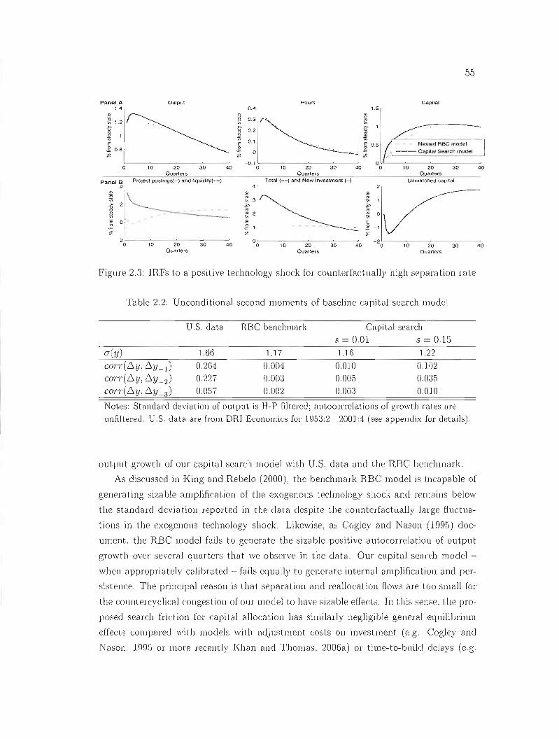
55
1.4 Panel A Oulpul Hours Capital
0.4 1.5
ni'" ni'"üi 1.2 <;;
-g ~
-g ~
~ 1 <;; '" 0.1E E Nesled ABC model g 0.8 g -J
-- Capilal Search model "if'
-- -0.1 o 10 20 30 40 0 '0 20 30 40 10 20 30 40
Quaners Quarters Quar1ers Panel B Project poslings(-) and tiquidiry(-) Total (--) and New Inveslmenl (-) Unmalched capilal
4
~ 3
-g ~
-g12\~ ID
!~~2l 0~ 2 Eg 0 g 1 -. j-1
"if' "if' -2o'------,0.,-----::20,------·30--~40 o --~------.- -2
o 10 20 30 40 0 10 20 30 40 Quaners Quarlers Quarters
Figure 2.3: IRFs to a positive technology shock for counterfactual!y high separation rate
Table 2.2: V nconditional second moments of baseline capital search model
D.S. data RBC benehmark Capital seareh
s = 0.01 s = 0.15 a(y) 1.66 1.17 1.16 1.22
cor-r(6y, 6y -1) 0.264 0.004 omo 0.]02
corr(6y,6Y_2) 0.227 0.003 0.005 0.035
corr(6y,6Y_3) 0.057 0.002 0.003 omo Notes: Standard deviatioll o[ output is H-P filtered; autoeorrelations o[ growth rat·es are
unfiltered. D.S. data are from DRI Economies [or ]953:2 - 2001:4 (see appendix [or details).
output growth of our capital search model with V.S. data and the RBC bcnchmark.
As discussed in King and Rebelo (2000), the benchrnark RBC lllode! is incapable of
generating sizab!e amplification of the exogenolls technology shock and remains below
the standard deviation reported in the data despite the counterfactllally large fluctua
tions in the exogenous techno!ogy shock. Likewise, as Cogley and Nason (1995) doc
ument. the RBC model fails to generate the sizable positive autocorrelation of output
growth over severa! quarters that we observe in the data. Our capital search model
when appropriately calibrated - fails equal\y to generate internai amplification and per
sistence. The principal reason is that separation and rcallocation flows are too slllall for
the countercyclica! congestion of our mode! to have siza ble effects. In this sense, the pro
posed search friction for capital 81\0cation has similarly negligible general equilibrium
effects compared \Vith models \Vith adjustlllcnt costs on investment (e.g. Cog!ey and
Nason. 1995 or more recently Khan and Thomas. 2006a) or time-to-build delays (eg.

56
Kydland and Prescott, J982) even though the qualitative implications of our model are
quite different.
2.5 Endogenous capital separations due to credit frictions
Different empirical measures suggest that credit frictions and thus capital separations
due to financiaJ distress are countercyclicaJ. Covas and Den Haan (2006), for example,
document that default rates for U.S corporate bonds peak at the end of recessions.
Likewise, we find that current liabilities of business failures taken from DRI (mnemonic:
fail) are countercyclica1 26 ParaJlel to Den Haan, Ramey and Watson's (2000) argument
that countercyclical job destruction implies substantiaJ propagation in a labor search
model, this suggests tbat extending our baseline mode] \Vith credit frictions such as to
generate countercyclical capital separations may, in fad, belp our capital search model
to generate more important business cycle effects.
As a l>y-producL, the extension also allows us to assess the role of costly capital
reallocation for the business cycle effects of credit frictions. In facto existing DGE models
with credit frictions such as Carlstrom and Fuerst (1997, CF henceforth) or Bemanke,
Gertler and Gilchrist (1999. BGG henceforth) exclusively focus on the effects of net
'North on investment and output. But since factors of production in these 1l10dels can be
moved costlessely From one finn to anotheL they abstract by definition from the effects
of capital reallocation due to financial distress.
2.5.1 Model extension
As in CF and BGG, we introduce credit frictions through a costly state verification
(CSV) mechanism originally proposed by Townsend (J 979). Finns are subject to an
idiosyncratic productivity shock that households (the côpitaJ lenders) can only observe
arter paying a monitoring cost. This assumption of asymmetric infofllliltioll implies that
in the absence of monitoring, the firm would always want to underreport its productivity
so as to avoid payment of the previously agreed upon rental rate. J-Iouseholds solve
this agency problem with a debt contract that specifies monitoring and default if the
idiosyncratic prodl1ctivity level of the finn falls below some optimal thresholcl.
While we follow the sallie CSV ôpproacb, our model differs from CF and BGG in
three important details. First. the optimal default threshold in our lIlodel is below the
~6ThE' [J-P flltered contemporanC'ous correlation of Covas and Den Haan's (2006) default rate \Vith real GDP is -0.33 for the period 19ï1-200'1. 3ncl -0.77 for the period J986-200tJ. The H-P Filtered correlation coefficient of our liabilities series \Vith real GDP is -0.33 for the sample 1948-1998 and -0.27 for the sample 1980-1998.

57
one in CF and BCC because capital n~allocation is costly in our model while in CF and
BCC, it is not. Second, we assume, as in the baseline mode, that firms transfer ail of
their profits to households at the end of the period. Hence, net worth - the channel
through which credit frictions affect investment in CF and BCC - is absent. Third, we
retain the assumption that the rentaI rate is determined so as to split the surplus of the
lending relationship. CF and BCC assume instead that the lending market is perfectly
competitive and thus, ail of the surplus goes to the firm.
The specifies of the extended modcl arc 8S follows. The representative firm's tech
nology becomes
(2.13)
where f(XtNt , Kt) describes the same constant-returns-to-scale function as before, and
al denotes the realization of the idiosyncratic productivity shock. ContraI')' to the ag
gregate shock Xl, which is known to ail participants at the beginning of the period,
the shock al occurs after ail optimal decisions have taken place and is only observed
by the finn. As in CF and BCC, we assume that at is independently and identical1y (12
distributed over time and follo\vs a lognormal distribution log(a) N( - IO~(Q), afog(a))rv
so as to ensure at E [0,00] and E(a) = 1.27
To deal with the asynnnetric information about finn productivity, households and
firms negotiate the rentaI rate Pl per unit of matched capital priar ta the realization
of at· If the finn makes positive profits (ie. if al 2 al where al is such that ad
(XtNl , Kt) - WlNt- PlKt - K:Vt = 0), the finn pays p,]{" the household refrains from
monitoring and the capital match continues. If, on the other hand, al < at the finn is
unable to pay the negotiated capital rentaI because we assume that the wage bill WlNl and the cost of posting vacancies K: vt need to be covered first in order for the finn to
continue operating next period. ln this situation, the hOllsehold pays the monitoring
cost to verify the firm's production and decides on the continuation of the capital match.
If al is above some optimal threshold Qt th8t wc derive below: the household takes ail of
the firm's production and covers for the totality of lVtNt and K:vt so as to continue the
capital match. If instead al is below the threshold Qt. the hOllsehold separates the match
and takes back its capital stock without receiving or paying anything. ln this case, the
firm is liquidated and the difference between production and the cost of WlNt and t,vt is
picked up by an insurance that is funded with the dividE'nds from profit-making firms 28
2ïThe assumption that al is independently and identicaJJy Jistributed in conjunction with const.antreturns-to-scale technology simplifies the analysis as we do not need 10 consider the history of shoeks incurred by each firm. Finn size th us rernains irrelevant. \l'hich is \l'h)' our notation continues ta abstract from firrn subseripts.
28See the appendix for the delails on this insurance. Suffiee to say here that wc implieitly assume
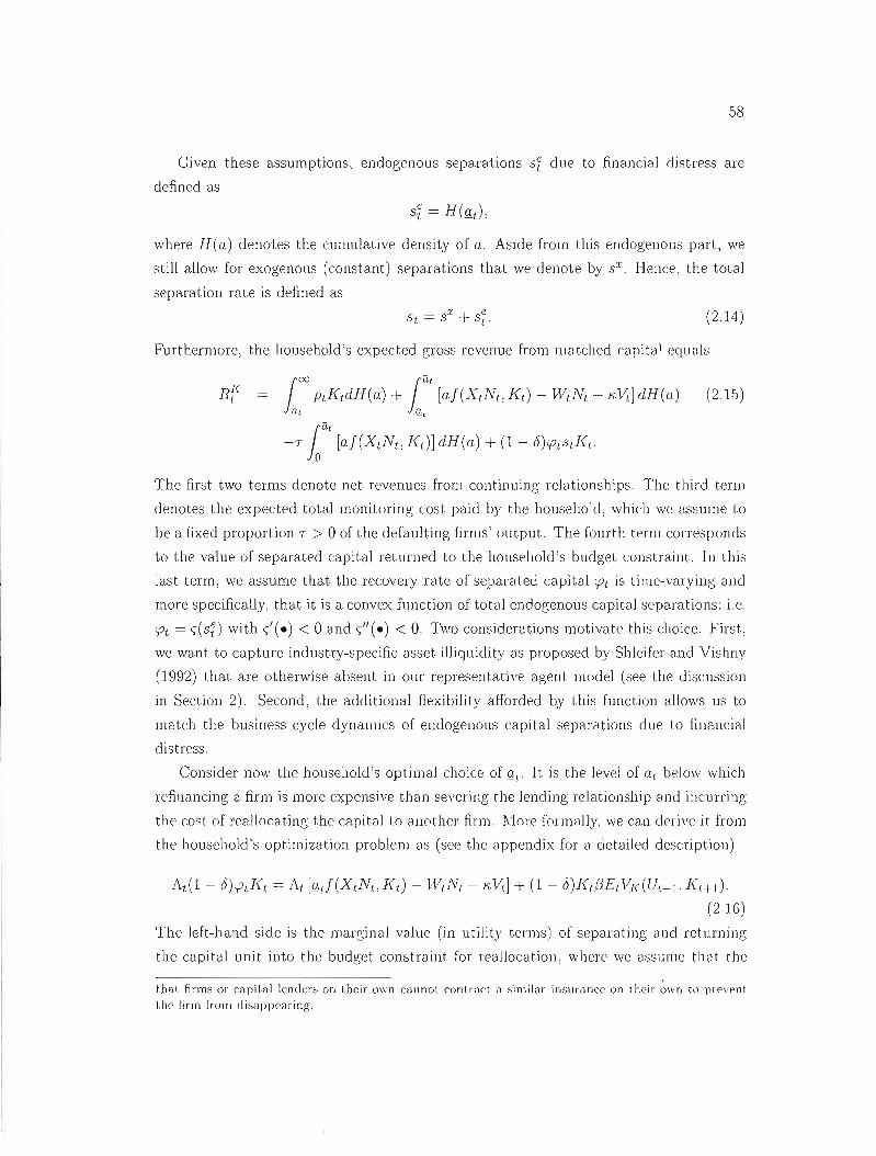
58
Given these assumptions, enclogenous separations si clue to fina.ncial nistress are
defined as
where H(a) denotes the cumulative density of a. Aside from this endogenous part, we
still allow for exogenous (constant) separations that we denote by sx. Hence, the total
separation rate is defined as
(2.14)
Furthermore; the household's expected gross revenue from matched capital equals
(2.15)
The first two terms denote net revenues from continuing relationships. The third term
denotes the expected total monitoring cost paid by the household; which wc assume to
be a fixed proportion T > 0 of the defaulting firrns' output. The fourth term corresponds
to the value of separated capital returned to the household's budget constraint. In this
last terrn, we assume that the recüvery rate of separated capital 'Pt is tilllc-varying and
more specifically, that it is a convex function of total endogenous capital separations; i.e.
<Pt = ç(si) with ç'(e) < 0 and ç//(e) < O. Two considerations motivate this choice. First.:
we want to capture industry-specific asset illiquidity as proposed by Shleifer and Vishny
(1992) that are otherwise absent in our representat1ve agent model (see the discussion
in Section 2). Second, the additional f1exibi]jty afforded by this function allows uS to
match the business cycle dynamics of endogenous capital separations due to finaucial
distress.
Consider now the household's optimal choice of Q:t. lt is the level of at below which
refinancing a firm is more expensive than severing the lending relationship and incurring
the cast of reallocating the capit81 to another firm. ]\'lore forll1ally, we can derive it from
the household's optimization problem as (see the appendix for a cletailed description)
At(1- 6)'PtKt = At [Q:t!(XtN1, Kt) - WIN, - K:V'i] + (1 - 6) Kd3Et 1IjdUt+l . K'+J)' (2.] 6)
The left-hancl sicle is the marginal value (in utility terms) of separating ancl rcturning
the capital unit into the budget constraint for reallocation: where we aSSUllle that the
that flrms or capital IcnJcrs on thcir own cannot conl rad il similnr insurancc on lhcir ~wn to prevenl
the firrn rrom disappearing.

59
representative household takes <Pt as exogenous. The right-hand side is the marginal
revenue from matched capital plus the marginal value of continuing the match into the
future. 29
Conditional on selecting a debt contract, the proposed monitoring and separation
scheme is optimal for both parties. The firm would not gain anything from reporting
output below what it actually produced because in case of monitoring, it will lose ail of
its output anyway. Likewise, the household would not gain anything from negotiating
a higher or lower auditing cutoff iit or a separation threshold Qt, by definition of the
utility-rnaximizing condition in (2.16).
Since any revenues associated with productivity shocks below at are absorbed either
by the capital lender (in case of continuation of the capital match) or by insurance
(in case of capital separation), firms now rnaximize only over the positive portion of
revenue net of current costs; i.e. foa; [af(XtNt, Ki) - PiJ(t - WiN!. - K;Vd dH(a). As
the appendix details, the first-order condi tions resulting from this objective function
would imply substantial over-hiring of labor relative to the RBC benchmark and thus
an unrealistically high labor share. We correct this implication by assuming, in addition,
that the representative firm in the extended model applies a constant markup Ill/; ~ 1
on its optimal decision problem.30
To close the model, "'le assume as before that the rentaI rate is determined by Nash
bargaining over the surplus of the capital relationship. This rentaI rate is nmv conditional
on the optimal Qi (see appendix)
Pt 'rJ [P(l,b.fK(XtNt : Kd + (1 - 8)(1 - St) ~ [1 - H(iii)]] + (1 - 'rJ) [8 + (1 - 8)(1 - tpdsd
+ [PiH(iit ) - (1 - 'rJ)(!:!:.i - Pi - T(1 - Pd).fK(XiNi,Kd] , (2.17)
where f-L = (00 adH(a) and Pi = (_CO adH(a) den ote partial expectations. COlllpared to -i J'dl Ja,
the case with exogenous separation, the first term in brackets is altered to reflect the
marginal product of capital and the saved sem'ch costs actually accruing to the Finn.
The third term in brackets represents the risk prernium that arises because households
29lt can be shown that Q1f(XIN1,J(,) < WtNt + "VI.; i.e. the household is \Villing to refinanee distressed firms up to a certain point so as to continue the capital match. This is because walking away from a relationship to reallocate capita.1 with another Firm is costly in the spnS0 thRt sepnrnted capital yielcls zero return in the nexl period and COoles \Vith the risk that remalching takes time. By contrasl, Jenders in the CF and BCC models never refinance since liquidating a defaliiting Finn and realJocating the capital is costless.
30 As proposed by Blanchard and Kiyotaki (1987), such a marktlp coulcl rpsull from a situation wiJere otherwise identical firms producE' imperfectly substitutabJe goods such l.hat each firrn races El
dowll\Vard-sloping demand in its relative priee.

60
do not receive the full contractual payment Pt (or even need to reinject money) and pay
monitoring costs when the firm's idiosyncratic shock drops below ii l .31
2.5.2 Calibration
To compare the extended model with the baseline model 10 which al! separations are
constant, we keep the common parameters unchanged in a first time; i.e. q = 0.5, s = 0.01, 'fi = 0.5, and E = 0.5. Further below, we perform robustness checks with respect to
alternative calibrations. The additional parameters requiring calibration are the markup
of price over marginal cost, 1/?/;, the fraction of output expended on monitoring, T,
the fraction of capital separations due to financial distress, se/s, and the elasticity
(orp/ose)/(se /rp) around steady state32
The crucial dimensions we want to match with our calibration are the relative im
portance and business cycle dynamics of capital separations due to financial distress.
Since the aJorementioned studies on firm-level capital fiows do not report such details,
we compute the relevant series ourselves from Compustat data (see the appendix for
a detailed description of the data). Specifical!y, we treat the following categories as
capitaJ separations due to financial distress: (i) exits due to liquidation (chapter 7); (ii)
sales during the years (-1 0 1 2) around bankruptcy filings (chapter 11); and (iii) sales
during the yeaTS (-1 0 1 2) around drops of more than 2 credit ratings in long tenn debt.
Compustat provides information on the reasons of exit for disappearing firrns as vvell as
information about debt ratings of continuing firms. To identify firm bankruptcies. we
link the Compustat database with information on chapter 11 filings from the Bankruptcy
Research Database.33 Total separations (defined as sales and exits) and retirements. in
turn, are computed as in Ramey and Shapiro (1998).34 Table 2.3 provides the thus
computed averages for the sample 1980-1993.35
31 BroadJy speaking, this risk pl'emium is the consequence of incomplete contracting in Cl world \Vith ex-post factor specificity that Williamson (1979) and more retently CabaJlero and Hammom (1996) term the fundamental transformation problem. The general equilibrium consequence is redllced AexibiJity of separation decisions and, in tum, a slower capital accu mlila tion process.
32Since we loglineal'ize the model, the other functional characteristics of <p = gIs") are irrelevant. 33The Bankrllptcy Research Database (BRD) is compiled by Lynn l'vi. LoPucki l'rom UCLA Law.
Of the 751 reported cases of bankruptcy filings by large publicly tl'aded firms sinee Oetober 1979. we were able to malch 623 firms with lhe unique firm identifiers used by Compllstat (mnemonic: gvkey).
3'!Ramey and Shapiro (1998) COllnt as total exits the ones related to mergers and liquidations bUl do not counl exits due to privatizations, level'aged buyouts and olher l'easons.
:J'J'vVe start the sample on]y in 1980 becallse, as Davis. Haltiwanger, Jarmin and l'diranda (2006) document, the proportion of medium-size and smaller firms listed publicly increascd importanLly in the early 1980s. This rnakes the Compustat sam pie more representative - especially \Vith regards exils due to financial distress. The end date 1993 is chosen because tller'eafter. I)I'I)1S no longer proviue accurate Illimbers for retirements, As mentioned before, Compustat data sholild be more representative fllr
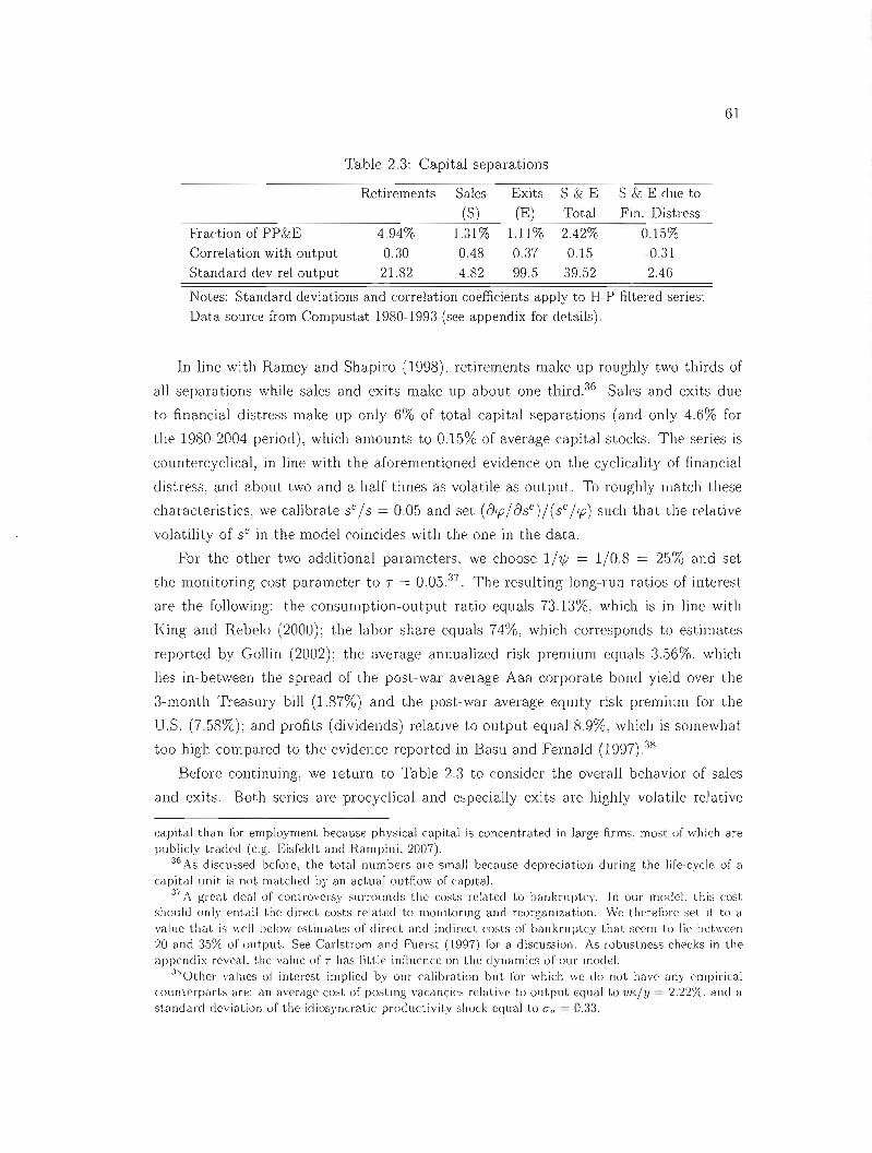
61
Table 2.3: Capital separations
Retirements Sales Exits S & E S & E clue to
(S) (E) Total Fin. Distress
Fraction of PP&E 4.94% 1.31 % 1.11 % 2.42% 0.15% Correlation with output 0.30 0.48 0.37 0.15 -0.31
Standard dev rel output 21.82 4.82 99.5 39.52 2.46
Notes: Standard deviations and correlation coefficients apply to H-P filtered series;
Data source from Cam pustat 1980-1993 (see appendix for details).
In line with Ramey and Shapiro (1998), retirements make up roughly two thirds of
ail separations while sales and exits make up about one third.36 Sales and exits due
to financial distress make up only 6% of total capital separations (and only 4.6% for
the 1980-2004 period), which amounts to 0.15% of average capital stocks. The series is
countercyclical, in line with the aforementioned evidence on the cyclicality of financial
distress, and about two and a half tilDes as volatile as output. To roughly match these
characteristics, we calibrate se /s = 0.05 and set (a<p/ase)/(se /<p) such that the relative
volatility of se in the model coincides with the one in the data.
For the other two additional parameters, we choose 1/7/) = 1/0.8 = 25% and set
the monitoring cost parameter to T = 0.05.37 . The resulting long-l'un ratios of interest
are the following: the consumption-output ratio equals 73.13%, which is in line with
King and Rebelo (2000); the labor share equals 74%, which corresponds to estimates
reported by Collin (2002); the average annualized risk premium equals 3.56%. which
lies in-between the spread of the post-war average Aaa corporate bond yield over the
3-month Treasury bill (1.87%) and the post-war average equity risk premium for the
U.S. (7.58%); and profits (dividends) relative to output equal 8.9%, which is sOll1ewhat
too high compared to the evidence reported in Basu and Fernald (1997).38
Before continuing, we return to Table 23 to consider the overall behavior of sales
and exits. Both series are procyclical and especially exits are highly volatile relative
capit.al than for employment because physical capit.al is concentrat.ed in large firms, most of which are publicly traded (e.g. Eisfeldt. and Rampini, 2007).
36 As discussed before, t.he t.ot.al numbers are smaJl because depreciat.ion during t.he life-cycle of a capital unit. is not. matched by an adual outflow of capit.al.
37 i\ great. c1eal of cont.roversy slIITounds the cost.s relat.ed to bankruptcy. In our mode!. t.his cost. should only entait the direct. cost.s related to monitoring and reorganizat.ion. Wc thereforc set il to a value t.hat. js weil below est.imat.es of direct and jndirecl costs of bankrupt.cy that. seem t.o lie bct.ween 20 and 35% of out.put.. See Carlst.rom and FUE'rst (1997) for a discussion. As robuslness ché'cks in t.he appendix reveal. t.he value of T has liUle innuence on the c1ynamics of our model.
3'Ot.her values of int.erest. impliecl by our calibrat.ion but. for which we do not. have any empiricaJ counlerpart.s are: an average cost of posting vacancies relative t.o out.put. equal t.o VK.jy:: 2.22<;':. and a standard deviation of t.he idiosyncrat.ic prodllct.ivity shock equal t.o (Jo = 0.33.
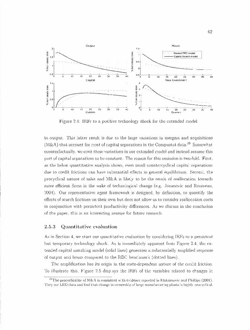
62
QUlpUI Hours 2 1.5
0.5o:------,~-,':-O-~,':-5--::2':-0--2'~5--.'30:---::'35=--~40 -0.5l------,~~:--~-~-_: o 10 15 20 25 30 35 40
Capital New Inveslment
'" 1.5 ;;; '" ;;; ~ 3
1
> 1
!':co 5 10 15 20
Quarlers 25 30
,=35 40
>u
'"* E 2 g, ...
20 Quarlers
25 30 35 40
Figure 2.4: IRFs to a positive technology shock for the extended model
to output. This latter result is due to the large variations in mergers and acquisitions
(M&A) that account for most of capital separations in the Compustat data.39 Somewhat
counterfactuaJly, we omit these variations in our extended model and instead assume this
part of capital separations to be constant. The reason for this omission is two-fold. First,
as the below quantitative ana.lysis shows, even small countercyclical capital separations
due to credit frictions can have substantia! effects in general equilibrium. Second, the
procyclical nature of saJes and M&A is likely to be the result of reallocation towards
more efficient firms in the wake of technological change (e.g. Jovanovic and Rousseau,
2004). Our representative agent framework is designed, by definition, to quantify the
effects of search frictions on their own but does not allow us to consider reallocation costs
in conjunction with persistent productivity differences. As we discuss in the conclusion
of the paper, this is an interesting avenue for future research.
2.5.3 Quantitative evaluation
As in Section 4, we start our quantitative evaluation by considering IRFs to a persistent
but temporary technology shock. As is immediately appa.rent from Figure 2.4, the ex
tended capital matching model (solid lines) generates a substantially amplified response
of output and hours compared to the RBC benchmark (dotted !illes).
The amplification has its origill in the state-dependellt nature of the credit friction.
To illustrate this, Figure 2.5 dispJays the lRFs of the variables related to changes in
39The procyclicality of l\ 1& A is consistent with evidellce reported in i\ laksimovic and Phillips (2001). They use LRD data and find th<lt change in ownership of large manufacturing plants is highly procycljcal.
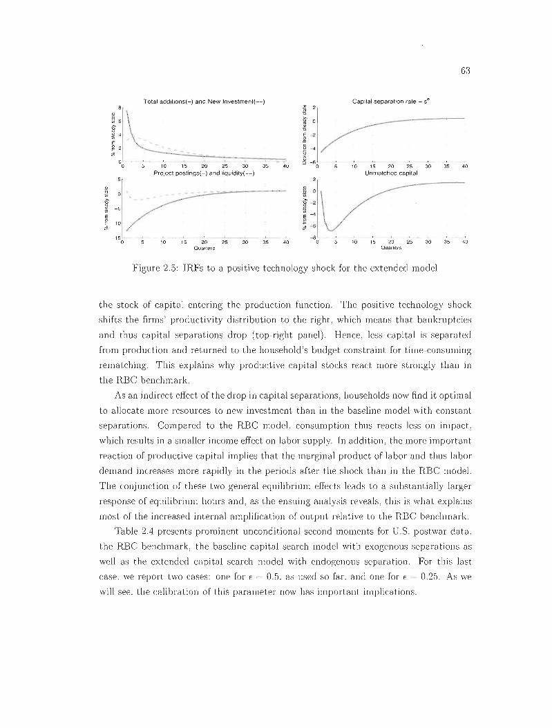
63
Tolal addilions(-) and New lnveslmenl(--) Capilal separahon raIe - se 8 v
~ >.
~ 0
'"E -2 g c .Q ;;;
-4
o o 5 10 15 20 25 30 35 40
~ -6 o 10 15 20 25 30 35 40
Project postings(-) and liquidily(--) Unmalched capital 5
v
* 0>. -g* -5 E o-= -10 oP
-15 . -8 o 10 15 20 25 30 35 40 o 10 15 20 25 30 35 40
Ouar1ers QuarletS
Figure 2.5: IRFs to a positive technology shock for the extended model
the stock of capital entering the production function. The positive technology shock
shifts the firms' productivity distribution to the right, which means that bankruptcies
and thus capital separations drop (top-right panel). Hence, less capital is separated
from production and returned to the household's budget constraint for time-consul1ling
rematching. This explains why productive capital stocks react more strongly than in
the RBC benchmark.
As an indirect effect of the drop in capital separations, households now find it optimal
to allocate more resources to new investment than in the baseline model with constant
separations. Compared to the RBC model, consumption thus reacts less on impact,
which results in a smaller income effect on labor supply. In addition, the more important
reactiol1 of productive capital implies that the marginal product of labor and thus labor
demand increases more rapidly in the periods after the shock than in the RBC mode!.
The conjunction of these two general equilibrium effects leads to a sl1bstantially lm"ger
response of equilibrium hours and, as the ensuing analysis reveals, this is what expJains
most of the increased internaI amplification of output relative to the RBC benchmark.
Table 2.4 presents prominent unconditional second moments for U.S. postwar data,
the RBC benchmark, the baseline capital sem'ch model with exogenous separations as
weil as the extended capital search model with endogenous separation. For this last
case. we report two cases: one for E = 0.5. as used so far. and one for E = 0.25. As we
will see. the calibration of this parameter now has important implications.

64
Table 2.4: Second moments for baseline calibration
V.S data RBC Capital seareh benehmark Exogenous Endogenous
E = 0.5 E = 0.25 a b a b a b a b a b
c 0.58 0.69 0.45 0.96 0.48 0.97 0.31 -0.38 0.33 0.85
n 0.95 0.87 0.29 0.97 0.27 0.98 0.63 0.97 0.40 0.97
k 0.28 0.10 0.28 0.14 0.30 0.44 0.25 0.10
~ 2.89 0.87 2.68 0.99 2.68 0.99 2.14 O.!YJ 2.,'5:3 0.99 se 2.46 -0.96 2.46 -0.96 2.46 -0.96
premium 0.54 -0.59 0.004 0.003 0.003 098 0.10 -0.97 0.03 -0.97
a(y) 1.66 1.17 1.16 1.71 1.28
Notes: (a) Standard deviation relative to output: (b) contemporaneous correlation with output. All moments are Hodriek-Prescott filtered. Data source from DR! Basie Economies 1953:2-2001:4 (see appendix for details).
Consider first the case where E = 0.5. As indicated by the IRFs; this version of
the extended model generates substantial amplification of output relative to the RBC
benchmark. As for persistence, howeveL the model still fails to generate the marked
positive autocorrelation of output growth that we see in the data (see Table 2.5 below).
The increase in internaI amplification is rooted in the general equilibriulll effects on labor
supply and labor demand that result in more volatile dynamics of hours. lntercstingly,
both the zero profit threshold at and the separation threshold Q:t are countercyclical,
which implies, in turn, that the model generates a countercyclical risk premium. AI
though the fluctuations of this premium are not as volatile in the data. this result is
a significant success of our extended model over the RBC benchmark as weIl as over
standard credit friction models without costly capital reallocation (see below)
Closer inspection of Table 4 reveals that the more volatile dynamics of equilibrium
hours corne at the cost of countercyclical consulllption. which is clearly at oclds with
the data. ln fact, the negative inCOllle effect brought about by the drop in capital
separations is so strong that households choose to decrease their consumption on impact.
These consumption dynamics hinge crucially on the elasticity E that links the matching 40probability q(Bd to the congestion measure Bt . For E = 0.5, the response of q(B t ) is
relatively large. 'vVe thus recalibrate E = 0.25 ~ü a~ tü rougbly match the consumption
dynamics in the data. The last columll of Table 4 reports the results. COllSlllllption is
4URecaii rrorn the first order condit.ion (1-3.12) that theexpected return rrom liquid ('apit;)1 is an average of the marginal values or matched and unmatched capital, weighted by the matching probability q(e). A stronger c.yclical response or q(e) means the average relurn to liquid capital rises more quickJy in an uplurn.

65
now procyclical and almost as volatile as in the data. The consequence of this adjustment
is a much smaller income effect on labor supply, which reduces the standard deviation
of output to 1.28 - a value just slightly above the RBC benchmark.
This exercise makes clear that the interplay between time-consuming capital (re
)allocation and countercyclical capital separation leads to amplification by affecting the
response of hours supplied by households. Exogenous shocks not only affect the factor
productivity as in the RBC benchmark, but also the stock of productive capital and
the amount of resources that need to go through the time-consuming allocation process.
The time-varying capital separation rate limits the income effect of rising returns to
capital, thus inducing households to shift more resources away from consumption towards
investment and supplying more homs. However, once we calibrate the model to yield
reasonable consumption dynamics, we find that these effects are modest and result only
in a small increase in internal amplification.
2.5.4 Volatility of separations and robustness to alternative
calibrations
As highlighted by the above results, a crucial ingredient for the marked internal propa
gation of our extended model is the income effect on labor supply whereby households
withhold current consumption to finance capital investments. The following robustness
checks assess to what extent alternative calibrations affect the performance of the mode!.
In ail of these exercises, we keep é = 0.25 so as to roughly match the consul1lption dy
namics in the data and adjust the elasticity (otp/ose)/(se /tp) such as to keep the relative
volatility of se consistent with the Compustat data. Table 2.5 reports the results.

Table 2.5: Sensitivity of model performance ta alternative calibrations
Baseline Mean allocation rate Bargaining power Separation rates
calibration q(8) = 0.25 q(8) = 0.75 7] = 0.45 7] = 0.75 se / s = 0.01 s = 0.02 a(y) 1.28 1.29 1.28 1.28 1.26 1.29 1.62 a (.c/) / a(y) 2.46 2.46 2.46 2.46 2.46 2.46 2.46 corr(se, y) -0.96 -0.97 -0.96 -0.96 -0.96 -0.96 -0.97
corr(6y,6Y_l) -0.004 -0.017 0.Ql0 -0.004 -0.002 -0.004 0.004 corr(6.y, 6y -2) -0.004 -0.013 -0.002 -0.005 -0.003 -0.004 -0.01
corr(6.y,6Y_3) -0.005 -0.010 -0.004 -0.005 -0.004 -0.005 -0.016
Notes: Standard c!eviations and cross-correlations are Hodrick-Prescott filtered.
Autocorrelations of growth rates are unfiltered.
ao ao
67
Changes in q (e) ,7] and se j s (keeping s = 0.01) have essentially no impact on the dy
namics of the model.41 This result would even hold if we didn't adjust (EJ<pjEJse)j(se j<p)
so as to keep u(se)ju(y) = 2.46. The reason for this robustness is that income effects
on labor supply remain small when E = 0.25 and capital separations on their own are
too insignificant to affect output significantly.
The dynamics of the model are more sensitive to changes in the average separation
rate s. For example, when we calibrate s = 0.02 pel' quarter (keeping se j s at 0.05), the
st.andard deviation of output rises to u(y) = 1.62. The mechanism for this incrcasc in
amplification is the same than before. The larger average s implies that the drop in sep
arated capital after a positive technology shock is more important and thus, households
di vert more resources away from consumption in order to achieve the desired amount of
liquid capital. The resulting negative income effect increases the volatility of hours, thus
leading to an amplified output response. As before, however, this effect is accompanied
by a negative correlation of consumption with output. If we correct this counterfactual
implication by lo\vering E even more, the amplification of output is rec\uced substantially.
Finally, it is interesting to note that there are several calibrations for which the
extended capital search model generates both important amplification and persistence
effects. For example, if we set the elasticity (EJ<pjEJse)j(se j<p) = 0 (i.e. <p is constant)
and E = 0.5, we obtain a(y) = 1.52, corr(6.y, 6.Y-l) = 0.28 and corr(6.y, 6.Y-2) = 0.08
without counterfactual consumption dynamics (see appendix for details). This marked
improvement in internaI propagation 1S due to an overly volatile endogenous separation
rate (more than a 1000 times as volatile than output). This illustrates that the combina
tian of search frictions for physical capital and countercyclical capital separations due to
credit frictions leads at least in principle to more important business cycle fluctuations.
The issue is sim ply that the flows of physical capital in and out of production are not
large and not volatile enough for the:,;e effect:,; to play a substantial role.
2.6 Conclusion
ln this paper. we examined the business cycle consequences of search frictions for the
allocation of physical capital The investigation is motivated by firlll- and industry
level evidence on market imperfections in the allocation of physicnl capital. Dcspite the
fundamentally diflerent nature of physical capital and labo!'. we argue that the market
imperfections involved in the allocation of these two factors are quite similar. Vie thus
"1 For the given calibrntion, lhere is no rational expcctations solution lo lhe model for values of T}
helu\\' OA5.

68
consider our paper as a first step towards analyzing capital allocation with the saille
type of search frictions that have proven fruitful for our understanding of labor markets.
By the same token, vve propose a complementary view to existing models of investment
that focus on aggregate adjustment costs and building delays in a wodd with perfect
markets.
The capital search model that we develop generates countercyclical congestion in
physical capital markets. in line with the data. Our analysis in a modern DGE context
suggests, however, that for reasonable calibrations, the internaI propagation effects of
these search frictions are modest. The main reason for this lad< of internaI propaga
tion is quantitative: separation and reallocation flows of physical capital are too small
for the search friction to play a significant l'ole. This conclusion remains intact when
we extend the model with credit market frictions that result in countercyclical capital
separations. While the combination of countercyclical separations and imperfect capital
(re-) allocation increases internaI propagation, alrnost ail of these effects stern from a
general equilibrium income effect that these frictions have on labor supply. Once we
tie down the mode] to generate consumption dynamics in line with the data, we find
that capital separations due to financial distress are sim ply not important and volatile
enough for them to generate significant internaI propagation.
Our results provide an interesting contrast to Den Haan, Ramey and Watson (2000)
who show that the introduction of countercyclica] job destruction in a labor search
model substantially magnifies and prolongs the business cycle effects of small shocks.
This difference in results is mainly due to the fact that labor is twice as important an
input to production as capital and that job destructions fluctuate on average much more
over the business cycle than capital separations. Furthermore. job destructions overall
are countercyclical while for capital separations, only the part linked to financial distress
is countercyclical. This part makes up only a sma]] fraction of ail capital reallocations,
which explains why its impact is so limited.
The comparison suggest that capital reallocations due to sales and l'vl&A are a more
important source of internaI propagation. From our firm-Ievel data, we know that most
capitaJ reallocations occur through these two channels and are substantially more volatile
than capi tal re81loca tions d LIe to fillé\l1cial distress. The problem is tha t sales and l'vl&A
are procyclical rather than countercyclical and tbus, they wOllld not generate more
important business cycle dynalllics in the proposed representative agent framework. At
the saille time, Jovanovic and Rousseau (2004) argue that sales and M&A of capital
are often the consequence of reorganization in the afterma th of elllbodied technological
progress. Hence. combining elllbodied technological progress in a heterogeneous firm

69
frame\~ork with search frictions for the reorganization of physical capital could entail
important interna] propagation effects as it takes time for firms and sectors to reallocate
factors of production to their most productive use.42
12 Andolfatt.o and i\lacDonakl (2006) propose a similar idea for the labor market to explain jobless rccover ies.

Chapter 3
Endogenous Flows of Foreign Direct
Investment and International Real
Business Cycles
Abstract
This paper models flows of foreign direct investment (FDJ) in a two country, t\Vo
sector DSGE framework. The allocation of capital to production capacity abroad
is subject to a search-and-ma.tching friction with endogenous capital reallocation.
The model is calibrated to observed gross inflows and outflo\Vs of FD! and leads
to dynamics of net foreign direct investment consistent with the empirical evidence
documented in this paper: inward and outward net flows of FOI are positively
correlated whereas a standard International Real Business Cycle model lIas the
prediction of a negative correla tion. r-.loreover; the model solves the aggrega.te
investment quantity puzzle as it generates cross-country correlations in-line \Vith
the data.
3.1 Introduction
Generally foreign investment is welcomed for bringing new capital to an economy and
increasing productivity through the nrrival of new technologies. This has also been
the main focus of the theoretical and empirical literatures concerned with foreign direct
investment. Little attention has been paid. however. to the short and medium run
behavior of foreign-controlled firnls and. in general. to their importance in unclerstanding
the business cycle of open ecollomies. This seems sOlnewhat surprisillg, as D cOllllnonly
uscd llle3sure of the rate at which foreigners gain control over a dOlllestic econOl1lY, ftows

71
of foreign direct investment (FDI), are large and very volatile. In Canada, for example,
foreign-owned firms generate up to one third of employment and control over a fifth of
ail assets, a share that has been stable over the last four decades l
The bulk of FDI, among developed countries, involves the replication of production
capacity abroad, or what is known as horizontal FD!' and in particular for the pur
pose of serving the host market (Brainard 1993, 1997). What is less weil known, and
is documented in detail for the case of Canada in Section 2, is that both net inflows
into, and outflows from, a host economy of FDI by foreigners increase during an up
tum. Moreover, business cycle fluctuations in net FDI in Canada and net Canaclian
investment abroad are positively correlatecl. Thus periods of increased net inflows into
an expanding economy are also periods of increased investment abroad by that same
economy. The classic international real business cycle, however, generates a negative
correlation between these flows.
The approach taken by this paper, in Section 3, IS to moclel flows of horizontal
foreign direct investment in a two-country, two-sector model,2 in which the allocation
of capital to production abroad is subject to a friction of the search and matching
type: bringing to fruitioll a new investment project abroad is costly and time c:onsuming
and, once in place, faces an endogenous termination probabiJity. The model therefore
provides a theoretical framework with endogenous gross inflows and outflows of foreign
direct investment in which congestion effects on foreign investment markets impact the
response of investment patterns to changes in productivity.
Several considerations motivate the modeling strategy adopted here. First, as argued
by Gordon and Bovenberg (1996), due to a lack of knowledge of the domestic economy
foreign firms are at a disadvantage in setting up and running a firm. While these
au thors capture this idea by assuming that output a t foreign firms is reduced by some
fixed proportion, the search and matching framework yields two distinct sources of costs
First: foreign firms expend more than domestic firms in bringing 8 new investrnent
project to fruition 3 Second, the probabilistic na ture of the ma tching proc:ess captures
IThese figures are for the manufacturing sector, see Ba.ldwin and Dhaliwal (2001) and Baldwin and Gellatly (2005). The importance of FOI does not limit itself to the case of Canada. For ex ample, the ratio of FOI to domestic investment in the US has risen From 6CX in t.he 1970s t.o 15% in the 2000s. Lipsey (2000) reports ratios above 10% for many indust.rialized country llver tbe period 1970 to 1995.
2This paper models horizontal FDI, treated in the trade theorv litera! url" by pa pers such as I\Jarkusen (1984), i\larkusen and Venables (2000), and Helpman, l\lelitz and Y('ôplC' (200<1). Dy opposition. vertical FDI refers to the "geographic distribution of production globall)' in response to the opportunities afTorded by different. markets." 1\lodels of the first category center around the "proxirnity-concentration" tracle-off, while the second are rnodels of factor proportions. Sec j\Iarkuscn (2004) for a good ovcrvic\V of the multi-national firm literature.
3Proximity-concentration models of FDI. e.g. Helpman, j\·lelitz and Ypaple (2004). generall.y assume

72
the fact that foreigners incur the cost of more time in setting up a new production fl'l-cility
or acquiring information about a risky investment project as in Gopinath (2004). 4
Quantitatively, the model generates the high cyclical volatility of net FOI flows, and
the positive correlation of net foreign direct investment inflo\vs and outflows observed in
the data. By contrast, a standard IRBC model with investment adjustment costs pre- ,
dicts a negative correlation, and lower volatilities of FOI flows. As Section 4 elaborates
in assessing the quantitative implications of the model, the allocation friction is central
to explaining the positive correlation of net inBows and net outflows of FDl. FoJlowing a
positive technology shock in the host economy, whether in a standard IRBC model with
investment adjustment costs or a search in FDI model with endogenous reallocation,
flows of net inward FDI increase on impact. By simple arbitrage, gross flows of FDI
from the host economy abroad decrease on impact, generating a negative correlation in
the standard IRBC mode!. However, in the proposed model this same drop in the pool
of capital goods available for allocation abroad increases the allocation probability for
the capital owner in the short l'un, thus mitigating the drop in new allocations abroad
and producing the positive correlation between inward and ou tward flows observed in
the data.5
Extending the model to allow for endogenous capital real!ocation, resulting from
the introduction of match-specific idiosyncratic productivity shocks, l'aises the positive
correlation between inward and outward net FDI even further. Drawing from the la bol'
market literature, starting with Mortensen and Pissarides (1994), reallocation occurs for
realizations of the idiosyncratic shock that yield a negative surplus to the relationship.
Following an expansionary technology innovation in the host economy, the opportunity
cost to the foreign capitallender of rnaintaining a unit of capita.l locked in with a foreign
afflliate increa.ses. This is because foreign affilia tes increase their project initiations faster
than foreign capital owners increase the pool of liquid capital available for allocation to
production abroad (i.e. to the expanding host economy). increasing the proba bility for
a given foreign capital lender of finding an appropriate investrnent projcct. Thus the
rate of capital reallocation from foreign affiliates increases with the host"s business cycle.
a fix cost to setting up operations abroad, above the the cost of entering the domestic market. As will be discussed beJow, foreign affiliates paya cost pel' investment project initiation. Although allocation or capital to clornestic Grms will be frictioniess. this is onl,)' a special case of the search envimnrllent when the initiation cost is nil.
4This setup was explored extensively in a closed economy setting for the allocation of physical capital by Kurmann and Petrosky-Nadeau (2009). Gopinath (2004) moclels the difficulty in acquiring tlte information on investment projects in ernerging projects as a time consuming search process.
'This is because, in this context;new allocations are a function of both the pool of capital availabJe and the allocation probability, or congestion on the foreign capital market.

73
This change in the gross Aow of capital from the expanding economy's direct investment
abroad further counters the drop in gross outflows.
This paper is related to the growing literature on international real business cycles;
dating back to the seminal contribution of Backus, Kehoe and Kydland (1992), and
to the transmission channels of international business cycles. One measure of the in
ternational transmission of business cycles, the cross-country correlation of aggregate
variables, poses a problem for standard IRBC models known as the quantity problem.6
That is, the ordcring of output and consumption cross correlations in the model is op
posite to that in the data. While many papers have made contributions to reducing or
solving this problem, few address another quantity problem involving aggregate hours
and investment.7 A result of focusing on net flows of FDI is that the model solves the
investment quantity puzzle. That is, contrary to other international real business cycle
model; the presence of congestions in foreign investment markets generates a positive
cross-country correlation of aggregate investment consistent with the data.
3.2 Flows of FDI and Canada - D.S. business cycles
This section reviews evidence on the cyclicaJ characteristics of FDl flows outlined lJ)
the introduction. While the Canadian economy is of particular interest for this study
because of the large and historically stable share of econornic activity originating in the
foreign sectoL it is increasingly significant for other industria.lized economies as they
further integrate. Flows of foreign direct investment into Canada; and flows of Canadian
direct investment abroad; concerning overwhelmingly the United States; the focus is
placed on the similarities and interclependence of both countries.
3.2.1 Canadian and D.S. business cycles
Despite a large difference in absolute size, in per capita terms the Canadian and U.S
economies are remarkably similar. The evolution of hours worked (indexed), real output;
investment and consumption per capita in both countries; over the period 1976-2006.
have but for a few episodes followed each other c1osely8 One example is the output per
capita gap between the U.S. and Canada appearing during the 19905. which also shows
up as a gap in average hours worked.
6Sec Backus, l<ehoc and Kydland (1995). "(Sep Crucini (2008) for an extensive survey. 8See appendix C for data and lechnical delails. The lime series lor the mentioned variables are
plot ted in Figure 1 of said appenu ix.

74
Table 3.1: Business cycle moments for Canada and the D.S
1976:1 - 2005:4 Canadian data 1 D.S. data 1 Cross-country variable: a b a b correlations Consumption 0.80 0.87 0.47 0.74 0.60 Hours 0.80 0.83 0.95 0.87 0.63 Investment 3.11 0.69 3.24 0.82 0.45 Output 1.53
1 1.42
1 0.75
a: Standard deviation relative ta output;
b: Contemporaneous correla.tion with output;
Al! moments are Hodrick-Prescott fiJtereeL
While aggregate trends have been similar, Table 3.1 examines differences in cycli
cal fluctuations of prominent macroéconomic variables, measured as 2nd moments for
Hodrick-Prescott filtered quarterly data over 1976:1 - 2005:4. The Canadian and D.S.
economies display approximately the same business cycle characteristics of these vari
ables: aJthough there is evidence of less aggregate consumption smoothing in Canada:
seen as the larger relative volatility of consumptioIl.9
One indicator of business cycle synchronization, the cross-country contemporaneous
correlation of prominent macroeconomic variables, is reported in the last column of
Table 3.1. In their extensive study of international business cycles, Ambler; Cardia and
Zimmermann (2004) find much lower, although positive, cross country correlations than
those for the Canada - D.S. pair, suggesting a higher than average degree of integra tion of
both economies. lO While both theoretical and empirical work have often followed trade
as a vector of synchronization: the increasingly important channel of flows of foreign
direct investment is explored in the next subsection ll
9See also Baxter and Crucin i (1995), Ambler, Card ia and Zimmermann (2004) for similar observations.
JO Ambler. Cardia and Zimmermann (2004) consider a sample of 20 industrialized countries, and ail pairwise cross-country correlations, on quarterly data over t.he period ]960:1-2000:4. Average output, consumption, investment and hours cross-correlations are, respectively, 0.22, 0.14, 0.18, 0.26.
Il Sales by multinational firms have outpaced the expansion of trade in manufactures over the last decades. See Markusen (2004). Kose and Yi (2001) explore and discuss the limitations of the trade approach to solving the quantity puzzles. Ambler, Cardia and Zimmermann (2002) explore the potential of il two country multi-sector mode! \Vith trilde in intermedinte goods in addressing the same issue. Other avenues have been expJored, such as variable capital utilization in Baxter and Farr (2005), or trade in capital goods in Boileau (1999). Jacoviel!o and i\!inetti (2006) explore the implications of imperfect cross-border credit relations for output cross-correlations. See also Schmitt-Grohé (1998) for an evaluation of various mechanisms.

75
3.2.2 Flows of FDI and foreign-controlled firms in Canada
There are essentially two ways in which foreigners can access a domestic economy: (i) by
establishing a branch or new business; (ii) through mergers and acquisitions of domestic
firms. A commonly usee! measure of the rate at which foreigners access a domestic econ
omy, flows of foreign direct investment, can further be categorized as either 'horizontal'
or 'vertical'. As described by Markusen (2004), horizontal FDI refers to the replication
of capacity abroad, and vertical FDI to the division of the production process globally in
order to exploit the benefits offered by different markets. As Brainard (1997) documents
and argues, the majority of FDI between developed countries is horizontal. In addition,
the large majority of foreign affiliate sales are destined to the host market12 There
rcmains, howcvcr, a debate over the principle mode of accessing an economy, although
Helpman, Melitz and Yeaple (2004) argue that it occurs mainly through 'greenfield'
investment. 13
ln order ta aSsess the extent and effect of foreign control over the national economy, in
1962 the Canadian government passed the Corporations Returns Act (CRA), requiring
firms doing business in Canada to report financial and ownership data. Of the 40000
reporting firms in 2004, foreign controlled corporations accounted for 30.7% of total
operating revenues and 28.5% üf aH assets held in Canada,14 shares that have historically
remained stable (see Figure 3.1)15 The United States plays a central role in the foreign
control of the Canadian economy, generating 62.6% of the operating revenues of foreign
controlled corporations. The c!osest behind are the United Kingdom and Germany with,
respectively, 7% and 6.5% of operating revenues.
By industrial sectoL foreign control is most important in oil and gas, manufacturing
and mining, and significant in wholesale trade, utilities, and transportation and ware
12 As reported in Brainard (1993), approximately 92% a foreign affiliate production in the United States is destined for the host market.
13By 'greenfield' investment, one refers to the estùblishment of ù branch or new business. The position taken by Helpman et al. (2004) difTers from that of Graham and Krugman (1995) ùccording to whom thp f'virlence is lf'sS df'flr and lf'ans rather towards a larger mie for mergers and ùcquisitions. While this paper will follow Helpman et al. (2004), it worth noting a recent contribution by Nocke and Yeaple (2007). These authors investigate the theoretical determinants of F'DI by III&A or green Field investment.
14 'The notion of control encompasses both direct and effective control. Direct contra! is defined a<; ù person, group or corporation holding, directly or indirectly, more than 50% of the voting eqllity. Effective control implies control through methods other th an ownership of the majority voting eqllity", sllch as when more than 50% of the directors of a corporation are ùlso directors of another corporation. A corpOl~ation is foreign controlled when either direct or eR'ecli"e control is held by ù persan. group or corporation not resident in Canada.' For additional information, see 'Corporations Returns Act. 2004.' catalogue no. 61-220. Statistics Canada. vol XI E, p. 3.
l'>This figure is reproduced from catalogue no. 61-220. Statistics Cùnacla, vol XI E.

76
Billions of dollars
40
Operating revenue
30
20 Assets
10
o '65 '70 '75 '80 '85 '90 '95 '00 '04
Year
Figure 3.1: Share of assets and operating revenue under foreign control. Source: Statistics Canada
housing16 Manufacturing stands out as a sector \Vith a large share of employment
and high degree of foreign control, involving nearly one fifth of employment and where
just over half of the revenues and assets are under foreign control. In fact, Baldwin
and Gellatly (2005) estimate the share of manufacturing employment originating in the
foreign sector to be 30% of total sectoral employment. Together, sectors with more than
20% foreign control, in terms of assets, involve 55% of employment. Although these are
not the ideal measures of aggregate activity generated in the foreign sector, they give a
sense of the importance of foreign controlled firms for aggregate outcomes.
3.2.2.1 Flows of foreign direct investment
Flo\Vs of foreign direct investment into Canada (receipts) and flo\V of Canadian direct
investment abroad (payments) from the Canadian Balance of Payments are large, his
torically around 20% of aggregate Canadian investment. The source and destination
of these flows is overwhelmingly the U.S., generating a share of 44% of receipts and
destination for 58% of payments. Exccpt for a bricf pcriocl in the carly lODOs, payments
have ahvays exceeded receipts. leading to a persistent c1eficit offset only by Canada's
historically positive trade balance (see Figure 3.2).
The business cycle component of net flows of FDI into Canada and flows of Canadian
direct investments abroad, along \Vith their cross-correlation are presented in Table
3.2. 17 Both flows are highly volatile. with H.-P. filtered standard deviations relative to
IGSee Table 2 of the appendix. The same figure also reports roI' these indust.ries their share or total employment.
J7]t is important to stress that Aows of portfolio invest.ment are excludcd. keeping only Aows of direct.

77
-7.5rr====,,-------,------.,------r-----,------,---, ~ .~ -8 () IL----x-'
~ -85
i:ï Il ..g Iii 1 <Il , -
~ -95~: ~ _10LL -'-I --l '-I ----l --'--I--'
1980 1985 1990 Year 1995 2000 2005
Figure 3.2: Flows of foreign direct investment receipts and payments, Canadian Balance of Payments.
Table 3.2: The business cycle of foreign direct investment.
1976:1 - 2005:4 Net Foreign Direct lnv. Net Canadian Direct in Canada Inv. Abroad
std. dev rel üutput 14.19 8.8 contemp.corr. with output 036 0.40
Ratio of inward to outward net FDl f10w standard deviations 0.62 Contemporaneous correlation, inward-outward net f1ows. 0.27
2nd moments were computed for Hodrick-Prescott Illtered data. Data source: Statistics Canada
output of 14.19 and 8.8, respectively. By comparison, the relative volatility of aggregate
investment is of the order of 3.11. Both net inflows and net outflows, that is net FDI in
Canada and net Canadian Direct Investment Abroad move strongly with the Canadian
business cycle, with respective contemporaneous correlations with Canadian GDP of
0.36 and 0.40. 1\'10reoveL Table 32 also reveals that net inward and net outward f10ws
are positively correlated. That is, periods of increased net inflows of FDI into Canada
are also accompanied by increased net Canadian direct investments abroad. This faet
has not received much attention; equilibrium models tend to predict that capital would
simultaneously f10w into high productivity and out of low productivity countries.
3.3 IRBC with search in FDI and endogenous reallocation
The moclel develops a framework with net illfJowS and net outflows of forcign direct
investment in a two country, two sector DSGE model. where gross investment flo\vs in
both directions evolve endogenously ,vith the business cycle. Each country is populated
investment.

78
by domestic and foreign firms and a representative hOllsphold. For simplicity the model
abstracts from trade in consumption goods. Households decide on optimal consump
tion, an aggregate of goods produced by both types of firms, and allocation of investment
goods to firms located at home or abroad. In order to initiate a new investment project
abroad, foreign affiliates must disburse a flow cost K,. This cost is paid until the project
is brought to fruition, a time-consuming task abstracted as a search and matching pro
cess with investment goods available for allocation abroad. No such friction applies to
changing production capacity at domestic plants locatcd in the home economy.18 Thus
domestic firms rent capital on spot markets while foreign affiliates choose the arnount of
new projects to initiate. Firms, dornestic and foreign, hire labor on competitive dornestic
markets.
As a matter of notation, the first country is referred to as the 'Home' country and the
second as the 'Foreign' country. Throughout, variables relating to the Foreign economy
will be distinguished by an asterisk. For example, kJdi denotes the stock of capital held
by foreigners in the 'Home' economy while kJdi* denotes the stock of capital held by
foreigners in the 'Foreign' country, i.e. held by residents of the Home country. We begin
by describing the friction to allocating physical capi tal abroad, domestic and foreign
firms, and then examine the problem faced by the representative household in the Home
ecollomy, the problem in the Foreign economy being syrnmetrical Endogenous capital
reallocation is introduced before c10sing the mode!.
3.3.1 Undertaking a foreign direct investment
In order to form a unit of capital abroad, a new projecL v, must be initiated at a
cost of K, by a foreign affiliate. 19 IvIeanwhile, a pool of liquid capital, l, must be made
available to be allocated abroad once the right location has been found. Tbis process
of matcbing new projects and liquid capital is abstracted by a constant returns to scaJe
rnatching technology m(v, l). Denoting e= t as a relative measure of capitalliquidity,
the probability for a given project initiation of becoming a productive unit of capital
in the current period is given by m~.1) = m(l,e) = p(e) , with op(e)jo(j > O. The
161n facto the frictionless capital market is a special case of the search environment with K = O. This extrcme assumption of no friction to allocating investmE'nt goods to domE'sLic firms at home is made for simplicity. As long as a\locating investment goods ()broad is relatively more costly than the ()\Iocation at home. the results go through.
'9This cost is reminiscent of Gordon and Bovenberg (1996) who assume that foreign investors, due to a lack of knowledge of the c10mestic economy, are at a disaclvantage in setting up ancl rUllning a Finn. They capture this iclea by assuming that output by foreign Drms is reducecl by some fixecl proportion. Gopinath (2004) assumes that investors in emerging markets must c1isburse Cl cost to acquirc information on investrnent projects whi]e the length of the acquisition periocl is subject to se3rch frictions.

79
equivalent probability for Iiquid capital is just m(~,l) = m(l/B, 1) = q(B), âq(B)/oB < O.
Once in place, a particular unit of foreign capi ta.l faces a probabili ty (the determi
nation of which is discussed later) St of being terminated. When this occurs the unit
of capital returns to the pool of liquid capital, net of depreciation, for reallocation. As
a result, the total amount of Iiquid capita.l available for allocation abroad in the current
period is defined as ·fdi ( J:) k fdi1t = 1t + 1 - U St"t + Ut, (31 )
where Ut = (1-q(Bt-d)lt- 1 is unmatched liquid capital from the previous period carried
forward with no !let return, and i{di are new investment goods added to the pool of Iiquid
capital.
These assumptions result in the following law of motion for the stock of foreign
capital in the Home economy
(3.2)
For ease of cornparison with the Balance of Payments, it is usefuJ to rewrite the law
of motion as k{~~ = (1 - O)k{di + m(vt, It) - (1 - 6)Stk{di. The expression m(vt: Id corresponds to gross inflows of foreign direct investment while (1-0)Stk{di corresponds to
gross outflows of foreign direct investment, the difference being net flows of inward FD!.
The Home economy's direct investment abroad is Iikewise decomposed into gross outflows
m(v;'ZZ) and gross infiows (1- O)s~k{di*(i.e.; returning from the Foreign country).
3.3.2 Domestic and foreign producers
Domestic and foreign firrns produce intermediate goods aggregated into a final hOl11o
geneous consumption good by an Armington (1969) aggregator Yt = C (Vf,y[di) = 1
[ç&(yf)l/ + (1 - ç&)(y{di)!I];;, with elasticity of substitution 7/) = 1/(1 - li) and relative
shares deterrnined by the parameter ç&. The relative price of the foreign finn's good is
then simply p{di = C 2 (vf, y{di) anJ that of the domestic firllI's good pZ = Cl (yf, y[di)
Domestic firms produce with technology vf = At(nf)I-O:(kfY', hiring both factors of
production from households on competitive markets. Optimization yields the following
two first order conditions:
pdyd(71-1) wd = (1 - O')_t_l. : (;3.3)t d
ni pdyd
(k1) rd = û_t_ t . (3.1 ) t kd . t

80
where wf and rf are, respectively, the remunerations of a unit of labor and a unit of
capital at domestic firms.
Foreign firms in the Home economy hire domestic labor, n fdi , and make capital
adjustment decisions by choosing the number of new projects to initiate, v, with the
production technology y{di = A t (n{di)1-O:(k{di)D:. This yields the foJJowing dynamic
program:
. [fdi . fdi fdi fdi .fdikfdi + (JE '\;+1 J(kfdi)]max Pt 'Ut - 7JJt nt - r t t - "-Vt t--. t+l f~ ,\"
nt ,Vt t
subject to k{:~ = (1 - 0)(1 - St)k{di + p(8t )Vt
fdi - A ( fdi)I-O:(kfdi)D:and Yt - t nt t
where w{di and r{di are, respectively, the remunerations of labor and capital at foreign
firms. The foreign affi]jate uses the stochastic discount rate ,GEt as aJl profits are'y;t
1
transferred to the foreign household. Optirnization yields the foJJowing two first order
condi tions:
fdi)(nt (3.5)
where Jkfd' (kt:;) is the marginal value of an additional unit of capital to the finn. While
the first condition is quite standard, sorne interpretation of the optimality condition for
project initiations is in order. This states thaL at the margin, the cliscounted expected
return to an additional unit of capital must be equal to the average cost of setting it up,
p(ê,)· As such. this may be interpreted as a "project creation" condition akin to the job
creation condition in labor search and matchillg models. Differentiating the finn's value
functioll: the miuginal value is defined as
f~ f~ ,\" (k fdi) - Pt Yt .fdi (1 ')( )(JE t+1 J (k fdi )Jkfd, t - 0: k{di - r t + - cl 1 - St t ,\; kf di t+ 1 •
ln combination with the first order condition for project initiations: this yields the
forward looking condition
,\" { fdi fdi }_J<i_ = .3E ~ Pt+lYt+l fdi (1 Â)(1 ) K (3.6)) 1 Xl'"~ (l: k fdi - rt+ 1 + - u - St+l (8 ) .p(B
1 . t+l P 1.+1

81
3.3.3 Domestic households
Households choose a level of aggregate consumption of the final homogeneous good,
hours to supply to both domestic and foreign employers, nf and n{di respectively, and
have two capital investment options: investing in firms at home, if, or investing in
capacity abroad, i{di*. ln addition, there are convex costs to producing new investrnent
goods (domestic and foreign) .20 The resul ting dynarnic program for the representative
household is thus
V(kf, k{di*, un = max . [ll(Ct ,l - nd + {3EtV(kf+l' k{~~*, U7+1)] Ct ,711 ,nfdl, i t ,ifdt"
subJ'ect t.o d d + fdi fdi + dk d + fdi*kfdi* + TI* _ . + dd + fdi*/fdi*wt nt wt nt Tt t Tt 't t - Ct qt Zt qt "t
and k{~~* = (1 - 0)(1 - 87)k{di" + q(8nl7
where nt = nf+n{d\ if = kf+l -(I-o)kf, and qf and q{di* are, respectively, the cost of
new investment goods destined for plants at home and abroad. Under the assumption .)
that the cost of adjusting physical capital is governed by the function <1>( b), as in t
Hayashi (1982), this priee is given by qi = [1>'(~ )] -1 , for j = d, fdi*, with <1>' (.) > 0
and <J!/1 (.) < 0; and such that in steady state q = 1. New investment goads destined for
foreign direct investment are defined as i{di* = lt - (1-0)87 k{di* -ur where (1-0)87 k{di*
is capital recouped from terminated operations abroad net of depreciation, and 11,7 are
units of investment goods not yet allocated. Again, l7 is thcrefore the total amollnt of
investment goods available for allocation to production abroad.
Denoting the multiplier on the budget constraint by Ât ; the optimality conditions
are
(cd llC(Ct. 1 - nd = Ât (3.7)
(nt) 1171d(Ct, 1 - nt) = Âtw1 (3.8)
(n{di) Unfd;(Ct: 1 - nd = ÂtWtfdi (3.9)
(if+ 1 ) Âtqf = ,6EtÂt+1 [rf+ 1 + qf+1 (1 - 0)] (3.10)
k fdi *(i{di*) \ fdi* j,J(JEt q [(8*)1,'vkf d .. (k d -t+1 : ut* +1/ltqt = t ~t+l' ) (3.11)
k fdi *(1 (8 *))11: (kd * )]+ - q t ·"'t+l· Hl' UH 1
The Euler equation far allocation of Îllvestment goods to damestic firms, eqllation (3.10),
has the llSllal interpretation of equating the opportunity cost of the investment. in
201t is weIl known (see Backus, J<ehoe and KydJand (1992). Baxter and CrllC:ini (Hl95)) that without an adjustment cost to the production of new capital goods the volatijity of new investment would be much tou large in this setting.

82
terms of current period forgone consmnption, to the expected return net of depreci
ation. The Euler equation governing foreign investment decisions, equation (3.11), has
a similar interpretation. The expected return, however, is an average of the marginal
values of matched (Vkfd'" (kf+l' k{:~*, u;+])) and unmatched (Vu' (kf+], k{:~*, 11;+1)) cap
ital, weighted by the matching probability q(en. The marginal values of allocated and
non-allocated investment goods are given by
v . (kd kfdü u*) À fdü. ut' 1. , t tqt ,
V (kd kfd'i* *) \ [fdi* f di*(l K) *] (1 "')(1 ·*)r<E Tr . (k·d kfdi * kf dù t, t , Ut At rt + qt - U St + - u - St fJ tVkf d,' t+l' 1+1
Since unmatched liquid capital yields no net retufIl, its marginal value is simply the
opportunity cost of funds. The marginal value of matcheù capital consists of the earnings
on the unit, r{di*, and the value of capital separated for reallocation net of depreciation.
The last term captures the continuation value if reallocation does not occur.
3.3.4 Repayment on foreign capital
Each unit of capital allocated abroad generates a surplus for the foreign affiliate and
the capital lender. The repayment on capital allocated abroad is deterrnined by Nash
bargaining over the total surplus generated by the relatiollship, defined as St = J(k{di)+ V fd;(kd' ,kfdi,Ut)- Vu (kd> .kfd'.utl. .. 21
k t t '\' t· 1 • ThIs results III the followmg repayment rule: t
fdi fdifdi _ Pt Yi
) f di - ( -) ( ) '" r t - 7]0 kf di + ( 1 - 7] qt 0 + 7] 1 - 0 1 - St et' (3.12) t
By the first tenn, the repayment is increasing in the marginal product of capi tal. The
second term captures the loss of value due to p!lysical depreciation, measureù by the
price of investment goods. the cost of which is split accorcling to the lender's bargaining
weight 7]. The long-tenu nature of the relatiollship is captureù by the final tenn. It
represents the initiation costs saved by the firm in the continued operation of the unit
of capital. By changiug the relative threat point of the finn in negotiations, a rise in '"
puts upward pressure on the repayment.
3.3.5 Endogenous reallocation and profits
As in lVlortensen and Pissarides (1994) for the labor market. the existence of a random
idiosyncratic productivity to the match is assumed. the realization of which occurs after
21The appendix provides details on the derivation of this repaymenl rule.
,ut* + 1) .

83
production decisions are made and factor price equilibria are established. Denote this
realization at > 0, where a is independently distributed over time with probability
density h(a), cumulative density H(a) and mean E(a) = 1, and folJows a log normal {J2
distribution log(a) rv N( - lo~(a), CJ?og(a)). The surplus generated by the relationship
between a foreign affiliate and the capitallender (i.e. the household) is then an increasing
function of this shock, S(at). Once the shock is observed, both parties discontinue the
match for realizations of at < {lt where {lt is define as S({lt) = o. Using a reslllt of Nash
bargaining, the separation threshold is defined by 22
fdi fdi f di Pt Y/. (-) ) K
TI. - {lt CX k fdi - 1 - 0 (1 - St p(B ) = 0 (3.13) t/.
fd, fdi In effect, the match is discontinued if the realized marginal product of capital at CXP / kf~;
1
plus the sem·ch cost saved by maintaining the current unit of capital is inferior to the
negotiated repayment. An increase in the average search cost p(~tl: for example, by
increasing the opportunity cost of exiting the match, lowers the separation probability.
FinaJ!y: an insurance mechanism fllnded out of profits l'rom continlling rclationships
is assumed in order to insure that ex-post the hOllsehold receives the fuIJ ex-ante return
to foreign capital, and that the fuJ! wage biIJ and costs of project initiations are covered.23
Thus aggregate profits returned to the hOllsehold are
100 [ fdi fdi fdi fdi fdikfdi -] dH( )IIt = aPt Yt - wt nt - Tt t - K-Vt a QI
Qt [ fdi fdi fdi fdi fdikfdi ] dH( )aPt Yt - w t nt - Tt t - K-Vt a (3.14)+lo . = fdi fdi fdi fdi .fdi 7jdiII t Pt Yt - W t nt - Tt 1\,/ - K-Vt· (3.15)
Eqllilibrium is defined by the system of equations (3.1)-(3.15), production technolo
gies for domestic, foreign firms and the final consumption good, and the dcfinition for
the separation rate, St = H({lt), in both the Home and Foreign cOllntries.
3.4 Quantitative results
The model is solved for the rational expectations equilibrilll11 of the log-lincar system
of eqllations \Vith the algorithm developed by King and Watson (1998). The quanti
tative implications are evaluated through impulse responses and llnconditional second
22See appendix for details.
23Gordon and Bovenberg (1996) use a sjmilar assurnpLion <'lbollt Lhe realization of an idiosyncratic produc:LiviLy shock, and use the law of large numbcrs Lo argue that thcre is 110 aggregaLe uncertainty. l-lere. an insurance funded out of aggregate profits is lIsed to address the issue.

84
moments. The results for Aows of FDI are discussed first, before looking at aggregate
variables and cross-country correla tions. In all instances the results are contrasted
with those for a standard IRBC with investment adjustment costs, and a model with
exogenous reallocation.24
3.4.1 Shocks and calibration
3.4.1.1 Extraction of a Solow Residual.
The underlying exogenous processes for technology, as in Backus Kehoe and I<ydland
(1992), is assumed stationary and to follow a VAR(l) process with possible cross-country
spill-overs. Parameter estimates are obtained by extracting Solow residuals for the
Canadian and U.S. economies and then estimating the following bivariate VAR(1):25
Pc,us
Pus
The results of the estimation are presented below for the period 1976:1 - 2005:4. As is
usual in this sort of estimation, the persistence parameter is very high. Also. as can be
gleaned from the covariance matrix, Canadian and U.S. innovations to the exogenous
process for technology are positively correlated. In a subsection below, the sensitivity
of the quantitative results to the specification of the exogenous process for technolog;y
will be examined.
0.9747 0.034 0.079 0.021]Pc pc.us] [ ] Residua]s Co",;ance ma<c;x' [ [ -0.0174 0.9264 0.021 0.05Pus c Pus
3.4.1.2 Calibration
The discount factor is set to {3 = 0.99 which corresponds to an average annllal l'cal yield
on a risk-less bond of 4.1 %. Preferences are separable in consumption and leisure, and
take the fonn u(ç[, 1-nt} = 10g(Ct)+ ;:V{1~~{-~. The parameter VJ is fixed sucb that the
average fraction of total hOUTS worked equals n = 0.2. Together \Vith ç = 4 this results
in a Frisch elasticity of labor supply of 1. Furthermore, the share dOll1estic goods in the
production of the final good, cP, is set such that the steady state equilibrium hours worked
2'IThe delails lhese models are presented in the appendix. It is important to note thal t.he firsl C0rresponds to the search model withoul allocation frictions, i.e. a mode] \Vith r.. = O.
2')Disembodied productivity is meDsured as a residual for a Cobb-Douglas production function: log(A,) = log(y,) - a:log(n,) - (J - n) log(k,). The f]lIarLp.rly sprips of an aggregatp C<1pital stock for
both economies is estimated using the perpelual inventory rnethod.

85
in the foreign sector are 1/4 of total hours, which is in the range of employment shares
reported earlier The share of capital in the production function is set to Cl' = 1/3, and
the rate of depreciation of capital to 8 = 0.025, which corresponds to an annual decline
of productive use of capital of 10%. The elasticity of the investment adjustl11ent cost is
0.025, within a range of values used in different studies (e.g., Baxter and Crucini, 1995;
Ambler, Cardia and Zimmermann, 2002, and Baxter and Farr, 2005), and is chosen to
match the relative standard deviation of aggregate investl11ent in the data. Finally, the
paral11eter 1/ in the Armington aggregator is chosen to imply an elasticity of substitution
between the foreign and domestic firms' goods of 15.
To calibrate parameters related to foreign direct investment, it is useful to let the
theory shed sorne light on the data. Recall the foreign capital accumulation equation
kJdi - ( r)k.Jdi . fi ' flt+1 - 1 - U t + In oWt - out OWt·
As the Balance of Payments provide information on foreign direct investment gross
inflows and outflows; given a rate of capital depreciation one can compute the im
plied foreign capital stock in the host economy, using the steady state property kJdi = [inflow - outflow] /8 to initiate the capital stock. It is then possible; using the time
series on ol1tflows, to obtain a Lime series for tlle reallocation rate as
outfloWt St = (1 _ 8)k{di'
resulting in a mean rate of S = 0.0602, an H.-P. filtered standard deviation relative ta
output of 145 and contemporaneous correlation with output of 0.16.
Next it is assul1led that it takes on average a little more than a quarter before
liquid capital is allocated and becomes productive; i.e. q(B) = 0.75, and the houschold·s
bargaining weight is set tü Ti = 0.5, in the miel-range of possible values.26 The final
pararneter left ta calibrate is the elasticity of the matching function; which is of the
fürm m(vt, lt) = (vd(lt)l-f. This parameter only influences the dynamics of the model
but does not affect the steady state: and is therefore selected such that the relative
volatility of the realloca tian rate s is close to the data; leading ta a choice of f = 0.8. A
sensitivity analysis of results to variations in these parameters is performed below.
\iVith these calibrations there is sufficient information tu enJogenously determill(~ the
rest of the paral11eters (i.e. B, K; a) such that the systenl of steady state equations is
26 As it is 'vell know that the resuJts of the search and matching model of equilibrium unemployment are sensitive to the value of this parameter (see Hagedorn and r..[anovskii. 2008) .. a series or sensitivitv test will be perrormed below.

86
Panel A Net lIows 01 FDI Flows 01 Dileet Inv. AblOad .15 4
f ;; ;;; .. Nel inward r.ows
101' --e- Net outward lIows
;;; ::~~ E 5
.·NewaIlOCalIOn!.gg
O~ ~ e~ -2r \~-~r~> .. . -4 r ReaUocations <!5 - .......e--- Nel oulward ~' . -6
o 10 15 20 25 30 o 10 15 20 25 30 Periods PeliOds
Panel B Neillows 01 FDI Flows 01 Dilect Inv. Abroad 10- 2
-5------------ 10 15 30 -3-----'-0---:'5--20-o 20 25 0 25 30
Periods PeriOds
Figure 3.3: IRFs to a positive "Home" sourced technology shock.
satisfied 27 The resulting long-l'un ratios of interest are the following: the consumption
output ratio equals 76.52% in line with King and Rebelo (1999); the labor share of income
amounts to 0.67, which lies in the range reported by Gollin (2002). Furthermore, this
calibration implies that the steady state ratio of net FDI to aggregate investment is i23%, that the average initiation cost relative to output equals VK./yfd' = 1% and that
the standard deviation of the idiosyncratic productivity shock equals (Ja = 0.27.
3.4.2 Flows of foreign direct investment
Figure 3.3 plots the impulse responses to a positive technology shock in the Home econ
orny of net inward and outward foreign direct investment for that expanding econoruy.
The significant difference between the responses of the proposed model (Panel A) and
an IRBC model with investment adjustment costs (Panel B), beyond their magnitude.
is the behavior of net outward flows (see circled line of panels A and B). In the search
model, outward flo\-vs drop progressively, whereas in the standard model the drop occurs
on im pact. l t is this diHerence tha t generates the posi tive cyclical correla tion of llet
imvard and outward flows that is a characteristic of the data.
To detail the response of net ol1tward direct investment flows, it is usefnl to recall
its definition as the diflerence between gross outflows and gross inflows from the Home
2iThe delails concerning the procedure for computing the steady state are available in the appendix.

87
to the Foreign economy:
Net outward : l~q(Bn - (1 - o)s~ k{di*
The second column of Figure 3.3 decomposes the response of net outward ftows into
these new allocations (dashed !ine) and reallocations (solid !ine) of capital abroad.28
Consider now what matters for the initial response of net outward FDI: the response
of gross outflows l;q(Bn and the reallocation rate si, k{di* being predetermined. As
the opportunity cost of capital abroad increases, households diminish thcir pool of liquid
capital l*: shifting resources to domestic firms, causing a drop in the Home country's
pool of capital available for investment abroad. This the only source of change in net
outftows in the model without allocation frictions, and therefore the drop in outward
FDI is immediate. When allocation frictions are present, however, the decline in the
pool of liquid capital is larger than the initial decline in project initiations at foreign
affiliates for two periods aJter the shock, leading to a short lived increase in the capital
allocation probability q(Bn 29 This reduction in market congestion counters sorne of
the drop in l* upon impact, and is seen in the muted initial decline in new allocations
abroad (see the upper right quadrant of Figure 3.3). As q(Bn declines thereafter, new
allocations attain their lowest 6 quarters following the shock.
The second distinction cornes from the effects on reallocation of capital already
abroad. As illustrated in the second quadrant of Figure 3.4, a positive innovation in
the Home country causes the reallocation rate in the foreign country to drop, reduc
ing the gross ftow (1 - 0)8; k{di* on impact 30 The drop pulls net outward ftows from
the Home the Foreign country upward, such that on impact net outward flows change
very little (again, see Figure 3.3). Thus the key to understanding the response of net
foreign direct investment flo\vs are the time-varying congestion, and to a lesser extel1t
reallocation rates, effects that are absent in the standard mode!.
IVlaking this point clearer. Table 3.3 present unconclitional second moments for ftows
of foreign direct investment in the data and generated by the competing 11l0dels. The
standard IRBC model with investment adjustment costs, for the reasons just outlined,
generates a strong negative contemporaneous correlation between net infiows and out
flows of FDI. A model \Vith constant, exogenous reallocation goes a long way in improving
28Note that the negative of gross inAows is plotted so as to better iJluslrate lhe positive impact of net outAows.
29J<urmann and Petrosky-Nadeau (2009) show that under relativel)' weak conditions, if preferences are additive and concave in cons\lmption for example. that congestion on the investment market will be increasing in the expecled growth rate of the marginal utility of consllmplion.
301'he contemporaneolls correlation \Vith the host economy's business cycle is 0.85 and its standard deviation relative to aggregate output J.13. 1'hese numbers relate to Hodrick-Prescott filtered moments.
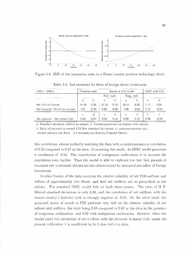
88
3 Home country separation rale Foreign country separation rate
~
;;; lnt 0.5
E 0 ~ c ~ -0.5
~ o
-1
-3 . o 5 10 15 20 25 30 o 10 15 20 25 30
Periods Periods
Figure 3.4: IRFs of the separation rates to a Home country positive technology shock.
Table 3.3: 2nd moments for flows of foreign direct investment.
1976: 1 - 2005:4 Canadian dat.a Search in FOI model IRBC with FOI
End. reall. Exog. reall.
a b a b a b a b
Net FOI in Canada 14.19 0.36 10.73 0.75 10.41 0.83 7.17 0.91
Net. Canadian Direct Inv abroad 8.8 0.40 8.83 0.06 7.08 -0.04 2.73 -0.54
c d c d c d c d
Net outward Net inward fOI 0.62 0.27 0.82 0.31 0.68 0.23 0.38 -0.58
a: Sta.ndard deviation relative to output; b: Contemporaneous correlation with output;
c: Ratio of outward to inward FDI How standard deviations; cl: contemporaneous corr.,
inwarcl-outward net Aows. Ali moments are Hodrick-Prescott filtered.
this correlation, almost perfectly matching the data with a contemporaneous correlation
of 0.32 compared to 0.27 in the data. Contrasting this result, the IRBC model genera tes
a correlation of -0.58. The contribution of endogenous reallocation is to increase the
correlation even further. Thus the model is able to replicate the fact that periods of
increased net investrnent abraad are also charactcrized by increased net inflow of foreign
investment.
Another feature of the data concerns the relative volatility of net FDI outflows and
infiows of approximately two thirds, and that net outflows are as procyclical as net
inflows. The standard IRBC mode! fails on both these counts. The ratio of H.-P.
filtered standard deviations is only 0.38, and the correlation of net outflows with the
source country's business cycle is strangl)' negative at -054. On the other hand, the
proposed model of scarch in FDI performs very weil on the relative volatility of net
inflows and outflows. the ratio being 0.68 compared 1.0 0.62 in the data in the presence
of exogenous reallocation. and 0.82 with endogenous reallocation. However, while the
model raises the correlation of net outflows with the dornestic business cycle. under the
present calibration it is insufficient to be in-line with the clata.
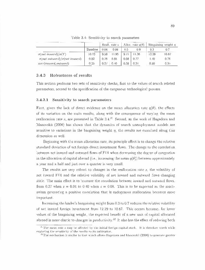
89
Table 3.4: Sensitivity to search parameters
Reall. rate s Alloc. rate q(fJ) Bargaining weight TJ
Baseline 004 0.08 05 0.9 03 0.7
<7(net inwaTd)/cr(Y) 10.73 9.58 11.95 971 11.36 12.29 10.67
CT(net outword)/CT(net inward) 082 0.76 0.85 0.98 0.77 1.40 0.78
corr(inwoTd, outward) 0.35 0.27 0.40 0.38 0.34 0.50 0.34
3.4.3 Robustness of results
This section performs two sets of sensitivity checks, first to the values of search related
parameters, second to the specification of the exogenous technological process.
3.4.3.1 Sensitivity ta search parameters
First, given the Jack of direct evidence on the mean allocation rate q(B), the effects
of its variation on the main results, along with the consequence of varying the mean
reallocation rate 5, are presented in Table 3.4.31 Second, as the work of Hagedorn and
Manovskii (2008) has shown tha t the dynamics of search unemploYlDent models are
sensitive to variations in the bargaining weight 1], the results are examined along this
dimension as weIl.
Beginning with the mean allocation rate, its principle effect is to change the relative
standard deviation of net foreign direct investment f1ows. The change to the correlation
between net imvard and olltward f10ws of FDl when decreasing the c1egree of congestion
in the allocation of capital abroad (i.e., increasing the mean q(B)) between approximately
a year and a haH and just over a quarter is very small.
The resul ts are very robust to changes in the reallocation rate 5: the vola tili ty of
net inward FDl and the relative volatility of net inward and outward f10ws changing
little. The main effect is to increase the correlation between inward and outward flows,
from 0.27 when 5 = 0.04 to 0.40 when s = 0.08. This is to be expcctecl as the mech
anism generating a positive correlation that is cndogcnous rcallocation becomes more
important.
Increasing the lender's bargaining weight hom 03 to 0.7 reduces the relative volatility
of net inward foreign investment l'rom 12.29 to 10.67. This occurs because. for lower
values of the bargaining weight; the expected benefit of a new unit of capital allocatecl
abroad is more elastic to changes in productivity.32 1t also has the effect of reducing both
31The mean rate s may be alTecterl by the initial foreign capital stock. lt is therefore worth \vhile exploring the sensitivity of the results to ils calibration.
32The mechanism is simiJar lo thnl which allows Hagedorn and l\Ianovskii (2008) to generate gre<lter
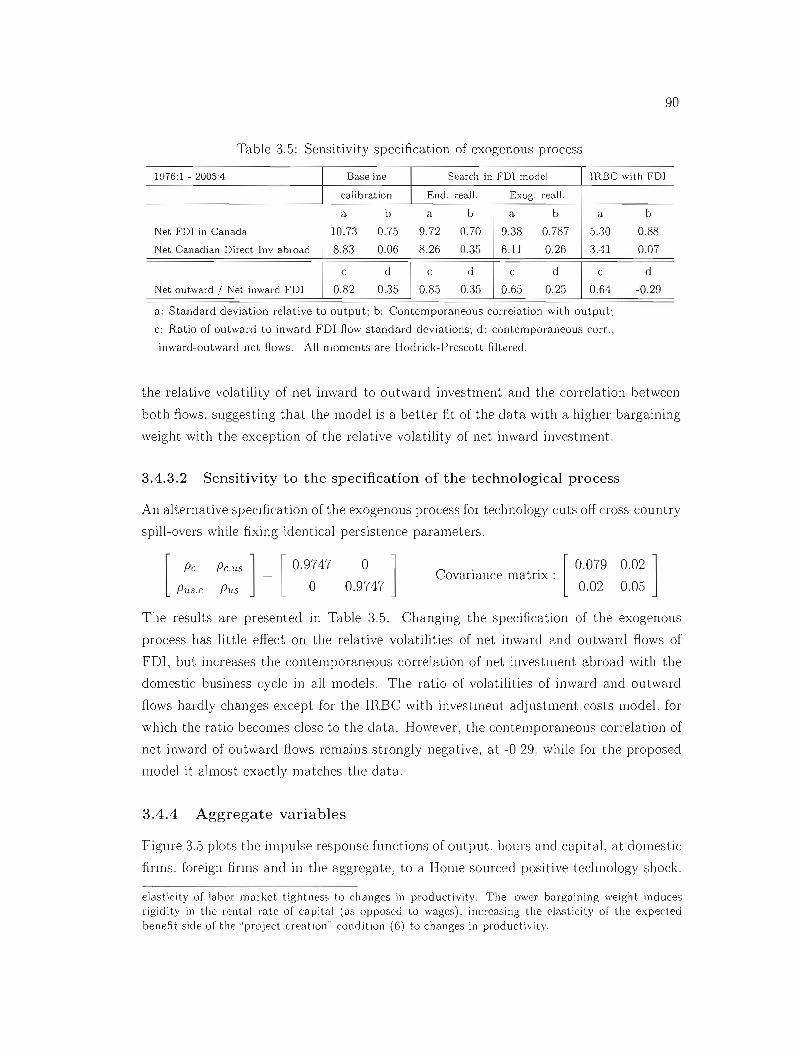
90
Table 35: Sensitivity specification of exogenous process
1976: 1 - 2005:4 Baseline Search in FD! model JRBC with FD!
calibration End. reall. Exog. reall.
a b a b a b a b
Net FDl in Canada 10.73 0.75 9.72 0.70 9.38 0.787 5.30 0.88
Net Canadian Direct lnv a.broad 8.83 0.06 8.26 035 6.11 0.26 3.41 0.07
c d c d c d c d
Net outward / Net inward FDI 0.82 0.35 0.85 0.35 0.65 0.25 0.64 -0.29
a: Standard deviation relative to output; b: Contemporaneous correlation with output;
c: Ratio of outward to inward FDI Aow standard deviations; d: contemporaneous corr.,
inward-outward net f1ows. Ali moments are Hodrick-Prescott filtered.
the relative volatility of net inward to outward investment and the correlation between
both ftows, suggesting that the model is a better fit of the data with a higher bargaining
weight with the exception of the relative volatility of net inward investment.
3.4.3.2 Sensitivity ta the specification of the technological process
An alternative specification of the exogenous process for technology cuts off cross-country
spill-overs while fixing identical persistence parameters.
Pc Pc.us ] = [ 0.9747 0 ] 0.079 0.02]Covariance matrix :
[ [Pus.c Pus 0 0.9747 0.02 0.05
The results are presented in Table 3.5. Changing the specification of the exogenous
process has little effect on the relative volatilities of net inward and outward ftows of
FDI, but increases the contemporaneous correlation of net investment abroad with the
domestic business cycle in ail models. The ratio of volatilities of inward and ou tward
flo-ws hardly changes except for the IRBC with investment adjustment costs model, for
which the ratio becomes close to the data. However, the contemporaneous correlation of
net inward of outward Hows remains strongly negative, at -0.29; while for the proposed
model it almost exactly matches the data.
3.4.4 Aggregate variables
Figure 3.5 plots the impulse response functions of output. bours and capital, at domestic
firms. foreign fions and in the aggregnte, to a Home sourced positive technology shock.
elasticity of labOT market tightness to changes in productivity. The lower bargaining weight induces rigidity in the rentai rale of capital (as opposed to wages), increasing the elasticity of the expected benefit side of the "project creation" condition (6) to changes in productivity.
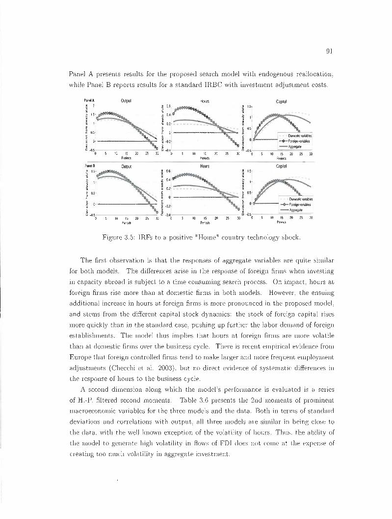
91
Panel A presents results for the proposed search model with endogenous reaJlocation,
while Panel B reports results for a standard IRBC with investment adjustment costs.
Panel A Outpul Hours Capnal ~ 2· * 0.6: ~"""'9&0_ ~ l.5r iii iii iii ~ 1.5" tJIP'''''"''''l9A.-. ~ 0.4: .. _.. ~ 1:
~ ~ : 1 Vi 1· (jj 0.21 iii E E E 0.5' ,g 05· ,g O·-------"II::-"".... ,g ccc
.~ O' --------=11......-: ~ -0.2' ~ O:If---
~ ~ ~ 0-0.5---------31 0 -0.4------- 0 -o.5---~=~~=
o 10 15 20 25 30 0 10 15 20 25 30 0 10 15 20 25 JO Periods Penods Periods
Panel B Output Hours Capital ~ 0.6' ~ 1.5'Ë 1.5",JjIJ_"'S!l",_ .
0; ~ _J1Illl"''tI8t~ ;; ~
~ ). fi O." ~~i 0.2' -----.::"la.. l 1·0;
E 0.5' E E 0.5' ,g ,g 0 --------::-.....=~ ~ Oomeslicvanables c c .~ Q' ---''"10- ~ -0.2' ~ Q. --9-Foreignvanables
~ ~ .~ - Aggregare
0-0.50---10--15--'20-2'--5---':30 0 -0"0 10 15 20 25 30 0 -0.50 10 15 20 25 JO
Periods Periods Periods
Figure 3.5: IRFs to a positive "Home" country technology sllock.
The first observation is that the responses of aggregate variables are quite similar
for both models. The differences arise in the response of foreign firms when investing
in capacity abroad is subject to a time consuming search process. On impact, hours at
foreign firms rise more than at domestic firms in bath models. HoweveL the ensuing
additional increase in hours at foreign firms is more pronounced in the proposed mode],
and stems from the different capital stock dynamics: the stock of foreign capital rises
IIIore quickly tbclD in the standard case, pushing up further the labor demand of foreign
establishments. The model thus irnplies that hours at foreign [irms are more volatile
than at domestic firms over the business cycle. There is recent empirical eviclence from
Europe that. foreign controlled finns tend to make larger and more frequent employment
adj ustments (Checchi et al. 2003), bu t no direct evidence of systematic clifferences in
the response of hours to the business cycle.
A second dimension along which the model's performance is evaluated is a series
of H.-P. filtered second moments. Table 3.6 presents the 2nd moments of prominent
macroeconomic variables for the three models and the data. Both in tenDS of standard
devia tians and correla tions wi th outpu t, ail three lllodels are silllilar in being close to
the data. with the weil known exception of the volatility of homs. Thus. the ability of
the lllOuel to generate high volatility in f10ws of FDI does not come at the expcnse of
creating too l1luch volcltility in aggregate investment.

92
Table 3.6: 2nd moments for prominent macro variables.
1976:1 - 2005:4 Canadian data Search in FDI model IRBC with FOI
End. reall. Exog. reall.
variable: a b c a b c a b c a b c
Consllmption 0.80 0.87 0.60 0.55 0.99 0.26 0.55 0.99 0.30 0.56 099 0.29
Hours 0.80 0.83 0.63 0.23 0.98 0.43 0.31 0.98 0.43 0.30 0.98 0.41
!n:l:estment 3.11 0.69 0,45 3.79 093 0.13 4.93 0.93 010 4.33 0.95 -009
Output 1.53 0.75 1.40 0.50 1.40 0.51 1.37 0.50
a: Standa.rd deviation relative to output; b: Contemporaneous correlation wiLh output
c: Cross country contemporaneous correlations. Ali moments are Hodrick-PrescotL filLerecl
A well know deficiency of standard IRBC models, the quantity problem, concerns
the ordering of cross country correlations of consumption, output; investment and hours.
The problem of the ordering of consumption and output cross correlations is the most
known of the quantity problems in the IRBC literature, as raised in the work of Backus,
Kehoe and Kydland (1995), while the shortcomings related to the cross correlation of
hours and investment have been raised in papers such as Ambler, Cardia and Zim
mermann (2004). Table 3.6 shows the performance of the search in FOI model with
this respect. All models get the ordering of a higher output than consulllption cross
correlations right, although the cross-correlation of consumpt-ion is lower than in the
data. This time on labor markets the three models perform quite well 33 However,
where aggregate investment is concerned, the cross-correlation is positive in both mod
els with search frictions in foreign direct investment; while an IRBC model with invest
ment adjustment costs generates a negative correlation. By altering the dynamics of a
component of aggregate investment; the time varying-congestion on foreign investment
markets resolves part of the investment quantity puzzle. Driving the point further; rais
ing the size of the foreign sector (as a fraction of total hours) from one quarter to one
halL l'aises the cross-country correla t-ion of aggregate investment from 0 13 to 0.20 in
the model \-vith search in FDJ; while the correlation is reduced from -0.09 tü -0.21 in the
standard IRBC mode!.
.J.JThis is clue, essenliaJly. lo the correlalion slructure lo innovations ancl the presence of investment adjustment Cüsts. This \Vas first poinlecl out by Backus. Kehoe and Kydland (1992); but made more cxplicil in Baxter and Crueini (1995).

93
3.5 Condusion
A commonly used measure of the rate at which foreigners gain control over a domes
tic economy, flows of foreign direct investment (FOI), represent an increasingly impor
tant share of aggregate investment in industrialized econoTlJies as they further integrate.
Given the importance of the foreign sector for aggregate outcomes and the relatively
high volatility of direct investment flows, quantitative models of open economies need
to be consistent with their dynamics.
As this paper has shown, a combination of frictiolls in the allocation of physical
capital to production abroad, and allowing for the endogenous reallocation of this capitaL
can replicate the positive correlation between net inflows and outflows of FOI that is a
feature of the data. ln addition the model can generate the higher volatilities of inward
and outward net FOL while the implication for prominent rnacroeconomic variables
are similar ta a standard IRBC model with investment adjllstment costs. HoweveL
there arp. important sp.<:toral difféences worth rnentioning in conclusion. The model
implies that, far example, hours warked at foreign establishments are more valatile than
hours worked at domestic establishments. An interesting questioll, and most relevant far
economic policy, is whether this is the case in the data. ln particlllar, if one considers the
extensive lllargin of l8bor adjustments, are jobs at foreign establishments more elastic
to the business cycle? JE so, this might offer a rationalization for the pu blic's skepticisHl
toward the benefits of increased foreign control of a domestic economy as emplayment
at these firms would be more fragile.

Conclusion
It has been argued that the standard model of equilibrium unemployment cannot gener
ate sufficient propagation as productivity shocks, by inducing a rise in wages, have little
effect on firm profits from a new employee and, hence, on the incentive to post new job
vacancies. The first chapter of this thesis has shown that when vacancies must be funded
in part on frictional credit markets, agency problems can lead to higher. time-varying,
unit costs that greatly increase the elasticity of vacancies to productivity. This propa
gation mechanism opera tes through two distinct channels: (i) a cost channel - lowered
unit costs during an upturn as credit constraints are relaxed increase the incentive to
post vacancies; (ii) a wage channel - the improved bargaining position of firms affordecl
by the lowered cost of vacancies limits part of the upward pressure of market tight.ness
on wages. The quantitat.ive exercise has shown that the cost channel is largely domi
nant in allowing the model to match the observed volatility of unemployment. vacancies
and labor market tightness. Moreover. the progressive easing of financing constraints to
innovations as firms accumulate assets generates persistence in the response of market
tightness and vacancies, a robust feature of the data and shortcoming of the standard
mode!. The paper thus concludes that the dynamics of vacancy creation costs are an es
sential element in understanding the cyclical behavior of job creation and the dYllamics
of the labor market Extending the model to allow for endogenous job separat.ion ilIl
provecl its ability to match gross labor flows statistics while preserving the propagation
properties.
Two questions J'emall1 and warrant further investigation in subsequent reseélfch.
FirsL how general these results are to the type of friction present on credit markets
is an open question. This call, however. be partially addressed by considerillg that an)'
friction which will generate a counter-cyclic:al c:ost exten18l funds will have the sallie
qualitative implications. Second, if hiring is conditional on the state of credit markets,
it may be that workcr flo\Vs. as opposed to investlllent in new capital goocls. are all
alternative channel for the transmission of rnolletaJ'Y policy shocks that affect the cost of
95
credit. This avenue seems particularly prornising as the propagation rnechanism in the
paper can be interpreted as increasing the rigidity of the firm:s marginal cost to changes
in production. Often referred in the New Keynesian literature as a greater degree of
real rigidity, this property is known to be essential for the dynamics of inflation and for
allowing any scope for monetary policy.
The second chapter examined the business cycle consequences of sear'ch frictions
for the allocation of physical capital. The investigation was motivated by firm- and
industry-Ievel evidence on market imperfections in the allocation of physical capital.
Despite the fundamentally different nature of physical capital and labor, it \Vas argued
that the market imperfections involved in the allocation of these two factors are quite
similar. This research is thus a first step towards analyzing capital allocation with the
same type of search frictions that have proven fruitful for our understanding of labor
markets. By the same token: it is a complementary view to existing models of investment
that focus on aggregate adjustment costs and building delays in a world with perfect
markets.
The capital search model generates countercyclical congestion in physical capital
markets: in line with the data: yet the analysis in a modern DSGE context sllggests that
for reasonable calibrations, the internai propagation effects of these search frictions are
lilodest. The main reason for this lack of internai propagation is quantitative: separation
and reallocation flows of physical capital are too small for the search friction to play a
significant role. This conclusion remains intact when the model is extended to credit
market frictions that result in countercyclical capital separations. While the combination
of countercyclical separations and imperfect capital (re-) allocation increases internaI
propagation: almost ail of these effects stem from a general equilibrium incol1le effect
that these frictions have on la bor supply. Once the model is tier! down ta generate
consumption dynamics in line with the data, capital separations due to finallcial distress
are sim ply not important and volatile ellough for them to generatc significéHlt internai
propagation.
These results provide an interesting contrast to Den Haan. Ramey and Watson (2000)
who sho\v that the introduction of countercyclical job destruction in a labor search
model subst.antially magnifies alld prolongs the business cycle effects of sllJaIl shocks.
This difference in results is mainly due to the fact that labor is twice as important of an
input to production as capital and thnt job destructions fluctuate on average much more
over the business cycle than capitnl separations. Furthermore, job destructions overnll
are countercyclical while for capital separations. only the part linked to finallcial distress
is countercyclical. This part makes up only a slllall fraction of ail capital reallocations,

96
which explains why its impact is so limited.
The final chapter has shown, a combination of frictions in the allocation of physical
capital to production abroad, and allowing for the endogenous reallocation of this capitaL
can replicate the positive correlation between net inAows and outAows of FDI that is a
feature of the data. In addition the model can generate the higher volatilities of inward
and outward net FDI, while the implication for prominent rnacroeconomic variables
are similar ta a standard IRBC model with investment adjustment costs. However,
there are important sectoral differences worth mentioning in conclusion. The model
implies that, for example, hours worked at foreign establishments are more volatile than
hours worked at domestic establishments. An interesting question, and most relevant for
economic poliey, is whether this is the ease in the data. In particular, if one considers the
extensive margin of labor adjustments, are jobs at foreign establishments more elastic
to the business cycle? If so, this might offer a rationalization for the public's skepticism
toward the benefits of increased foreign control of a domestie eeonomy as employment
at these firms would be more fragile.

Appendix A
Credit, Vacancies and
Unemployment Fluctuations
A.l Data sources
Table A.l: Data sources
.lob vacancies Conference Board Help-Wanted Index
Unemployment rate B.L.S. series LNS14000000
.lob nnding rate F'ujita and Ramey (2008) based on C.P.S. data
Output Expenditure based, 2000 chained dollars, B.E.A.
Yield Spreads l'v1oody's Seasoned Aaa and BM Corporate Bond YielcL DRl datnbnse
with 3-month U.S. Treasury bills, from FRED JI
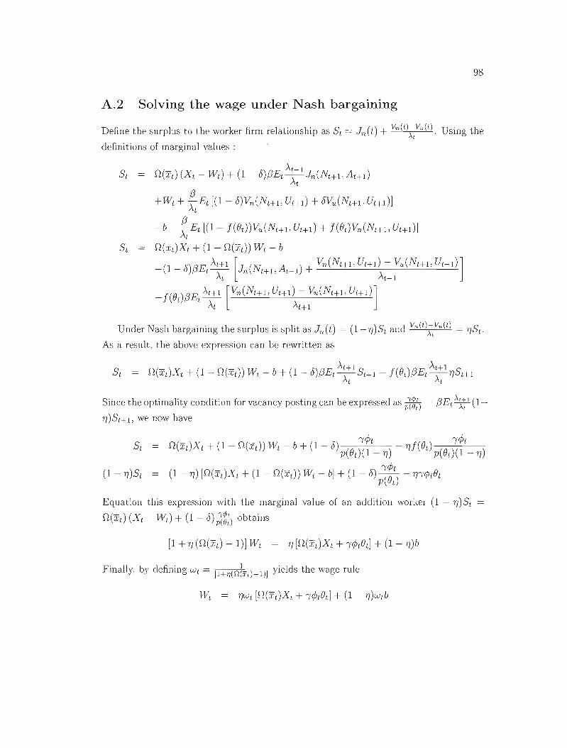
98
A.2 Solving the wage under Nash bargaining
Define the surplus to the worker-firm relationship as St = Jn(t) + v,,(t)~Vu(t). Using the
definitions of marginal values:
Àt+1St = D(xt)(Xt - Wt) + (1- 8),6Et----;::Jn(NH1:AH1)
+Wt + ~t Et [(1 - 8)Vn (NH1l Ut+1) + 8Vu (.NH1 :Ut+1)]
-b - ~ Et [(1- f(8t ))Vu (Nt+1 : UHd + f(8 t)VnCNt+1, Ut+d]
St = D(xt)Xt + (1 - D(xd) W t - b
- 8)6E ÀH1 A ) + Vn(NHJ : UHJ ) - ~L(Nt+l: U(1 )]+( 1 , t \ [Jn(Nt+ 1 : t+ 1 \At At+l
_ f(8 )6E Àt+1 [Vn(Nt+! l UHd - Vu (Nt+1:Ut+d] . t, t \ \
At At+l
Under Nash bargaining the surplus is split as Jn.(t) = (l-rJ)St alld Vn(t);:Vu(t) = 1]St.
As a result, the above expression can be rewritten as
Since the optimality condition for vacancy posting can be expressed as i(::) = ,6Et \~ J (1
1])St+l, we now have
D(xt)Xt + (1 - D(xd) Wt - b + (1 - 8) (8 ~<Pt ) - 1]f(8d (8 ~<Pt .)P t 1 - 1] P t 1 - "1
(1 -1])St (1 -1]) [D(xt)Xt + (1 - D(xt)) Wt - b] + (1 - 8) P~~:) -1]icPt8t
Equation this expression with the marginal value of an addition worker (1 - rJ)St =
D(Xt) (X t - Wd + (1 - <5) Ptt) obtains
Finally: by defining Wt = [I+IJ(ll(xtl-I)] yields the wage rule
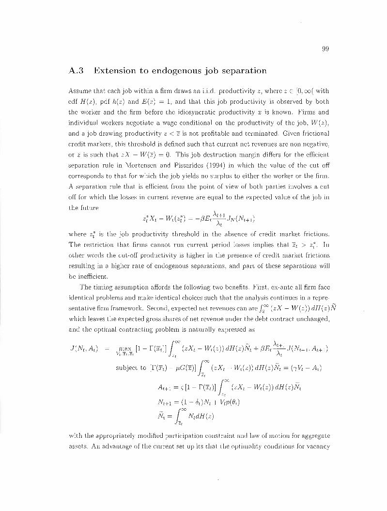
99
A.3 Extension to endogenous job separation
Assume that each job within a firm draws an i.i.d. productivity z, where z E [0, oo( with
cdf H(z), pdf h(z) and E(z) = 1, and that this job productivity is observed by both
the worker and the firm before the idiosyncratic productivity x is known. Firms and
individual workers negotiate a wage conditional on the productivity of the job, W(z),
and a job drawing productivity z < z is not profitable and terminated Given frictional
credit markets, this threshold is defined such that current net revenues are non negative,
or z is such that zX - W(z) = O. This job destruction margin differs for the efficient
separation rule in Mortensen and Pissarides (1994) in which the value of the cut off
corresponds to that for which the job yields no sUJ'plus to either the worker or the firm.
A separation ru le that is efficient from the point of view of both parties involves a cut
off for which the losses in current revenue are equal to the expccted value of the job in
the future
* W ( *) f3 Àt+l ( )Zt X t - t Zt = - Et~JN Nt+ 1
where z; is the job productivity threshold in the absence of credit market frictions.
The restriction that firms cannot l'un current period losses implies that Zt > z;. ln
other words the eut-off productivity is higher in the presence of credit market frictions
resulting in a higher rate of endogenolls separations, and part of these separations will
be inefficient.
The timing assumption affords the following two benefits. First, ex-ante ail firm face
identical problems and make identical choices such that the analysis continues in a repre
sentative finll framework. Second, expected net revenues can are J'Zoo (zX - W(z)) dH(z)N
which leaves the expected gross shares of net revenue under the debt contract unchangcd,
and the optimal contracting problem is naturnlly expressecl as
oo À n~a~ [1 - f(l'dl (zXt - Wt(z)) dH(z)Nt + (JEt ~J(Nt+l' At+ 1)
V/.x/.z/ . ~ Ii Àt
subject to [f(Xt) - j.LG(l')] ~cc (zXt - Wt(z)) dH(z)Nt = (jVt - AdJIt
At+1 = ç [1 - f(l't)ll~ (zX 1 - Wt(z)) dH(z)Nt
Nt+1 = (1 - odNt + Vtp(e t )
Nt = (CC NtdH(z)JIt
\Vith the appropriately modifjed participation constraiIlt and law of motion for aggregate
assets. An advantage of the current set up its that the optimality conditions for vacancy

100
postings and the monitoring threshold retain the same form as earlier. Closing the
extension to endogenous job separation, the intertemporal vacancy condition is now
"tcPt 1 [ _ ~(X) "tcPt+l ]-(e) = --Et [1 + D(XHl)] (zXt+1 - WH1 (z)) dH(z) + (1 - Ot+d (e ) p t 1 + Tt Zt+! P t+ 1
and the negotiated wage
Had the eut-off value of the job productivity eorresponded to that for which the
value of the job to the firm is equal to zero, the job destruction margin would have been
expressed as
Using the same notation as earlier, D(Xt) = cPt [['(:rd - I-tG(:rdJ - ['(:rd, the separation
condition wouId have been
and is interpreted as the job productivity at which the current revenue generated by
the worker net of his cost is equal the present discounted value of the worker in the
future. Using results from earlier, in the absence of monitoring cost this collapses to the
familiar
- X W' (-) Î'Zt t - t Zt = p(e )
t
Appendix B
Search i11 Physical Capital Markets
as a Propagatic~n Mechanism
This technical appendix presents the full details of the extended capital search model
"vith endogenous separation due to credit market imperfections. It also describes a
scenario with the matching friction removed. Results for an extensive sensitivity analysis
of the models with exogenous and endogenous separation are provided. The propagation
potential of endogenous separation is illustrated before discussing the data used in this
paper.
B.l Model
As in the frictionless RBC benchmark, our model is populated by two agents: firms that
produce using capital and labor; and households who decide on optimal consumption.
leisure and investments in either risk less bonds or productive capital
\"le add two frictions to this benchmark. First, the allocation of capital from house
holds to firms involves a costly and time-consuming matching process. Second: the
capital lending relationship between households and firms is subject to a credit market
friction. Following the costly state verification Iiterature initiated by Townsend (1979),
this credit market friction takes the form of an idiosyncratic productivity shock that
households can only observe at a cost. This asymmetric information assumption gives
rise to an agency problem that results in a debt contract with endogenous separation of
capital from firms whose productivity falls below a state-dependent threshold.
For the sake of simplicity; the model abstra.cts from a numbcr of potentially impor
tant factors that deserve to be mentioned. First. there is no distinct sector for capital

102
allocation Instead, households act directly as capital lenders. Second, firms transfer ail
of their profits to households at the end of the period. Bence, net worth - the chan
nel through which credit frictions affect investment in the existing financial accelerator
models - is absent. Third; the same matching friction applies to the allocation of both
new and used (i.e. previollsly separated) capital. This assumption simplifies our model
because we do not need to keep trac!, of different types of capital. Fourth, we do not
distinguish among different firms because, as discussed below, our modeling assumptions
imply that ail finns are identical and that finn size is indeterminate.
B.l.l Search and matching in the capital market
Capital is either in a productive state or in a liquid state. We define by Kt the capital
stock that enters the production function of a representative finn in period t. Liquid
capital L t , in turn, is made up of two components: used capital that has been separated
previous)y from other firms and new capital made available by households.
To undertake investments, firms must post projects and search for liquid capital at li
cost of r;, per project. We denote by iIt the number of posted projects of a representative
Finn in period t. Actual investment (i.e. new capital allocations) in period t then is the
result of a matching process m(Lt , Vi.) that is a positive function of the total amount
of liquid capital Lt and the total number of project postings Vt. A firm's probability to
find capital is therefore given by p(et) = m(~:Ltl with 8p(et)/8et > 0, where et = ~: is
a measure of capital market liquidity. Likewise, the probability of liquid capital being
matched to a firm equals q(et) = m(~:Ld with 8q(et )/8et < 0 1
Capital matched to a Finn in period t - 1 enters production in period t. This rela
tionship between finn and capital continues to hold in t +1 with probability (1 - St) and
so on for the periods thereafter. If the relationship is terminated, which happens with
probability St: the capital is separated and returned to the household net of depreciation
8. Both the matching probability and the separation rate arc taken as exogenolls by the
Finn but depend on the state of the economy, as will be described below. Given these
assumptions. the evolution of the productive capital stock is described by
(B.l )
Iln addition, to ensure that p(Bd and q(BI ) are bet.\\"een 0 and l, we require that m(L/. VI) ~
min[L i , VI]

103
B.1.2 Firms
At the beginning of each period, firms and households observe exogenous aggregate
technology X t . Given the existing capital stock Kt, a firm then posts new projects lit at unit cost '" and hires labor Nt at wage rate Wt to produce output Yt with technology
(B.2)
with fN, fK > 0 and fNN, h(K < O. The variable at > 0 oenotes the rea!ization
of an idiosyncratic productivity shock that is independently distributed over time with
probability density h(a), cumulative density H(a) and mean E(a) = 1. This shock
occurs aI'ter ail optimal decisions have taken place and aI'ter the factor price equilibria
are established.
Given these assumptions: the profit maximization problem of the finn is described
by the following Bellman equation
J(Kd
s.t. Kt+l
where Pt is the rentaI rate of capital; and {3Et I\;t is the discount factor of future
cash flows. Several comments are in order about this expression. First: the discount
factor is a function of the marginal utility of consumption II. because the finn trans
fers ail profits to the household. Second: the firm maximizes only over the portion
of the revenue net of capital rentaI costs for which it is expected to retain profits:
IoC; [?j)af(XtNt, Kd - PtKt - WtNt - "'lit] dH(a), where at is defined as the break-even
point associated with zero profits; i.e. at such that ad(XtNt:Kd = PtKt + WtNt + ",Vt·
As explained below: this is because under optimal contracting: any revenues associa ted
with productivity shocks below at are absorbed either by the capital lender (in case of
continuation of the capital match) or by an insurance (in case of capital separation).
Third: we assume that firms are 1l10nopolistic competitors and apply a consümt markup
1j'I/J :2 1 on their optimal decisions. This addition is necessary because the firm's opti
l1Iization over the range lat: 00] by itself would result in substantial over hiring relative
to the RBC benchmark and thus a la bol' share tha t is too high. Four th . the Finn takes
both HI! and Pt as exogenous. The exogeneity of Hlt is a direct consequence of our
assurnption of competitive labor markets. The exogeneity of Pt: in turn. implies that
firllls in our model do not intemalize the effects of their capital stock on the marginal
productivity of capital and thus on the negotiation of Pt discussed below.
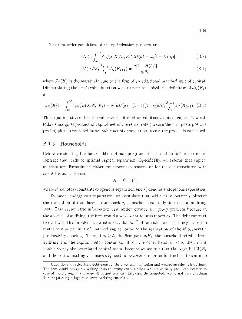
104
The first-order conditions of the optimization problem are
00
(Nt) :1 1JafN(XtNt:Kt)dH(a) = will - H(adJ (B.3) at
(V,) . {JE AI,+l J (K ) = ,..[1 - H(al,)] (BA)t· t At K t+1 p(Bt )
where JK (K) is the marginal value to the firm of an addi tiona! matched uni t of capi ta!.
Differentiating the firm's value function with respect to capital, the definition of JK(Kd
is
This equation states that the value to the fifln of an additional unit of capital is worth
today:s marginal product of capital net of the renta! rate (in case the finn posts positive
profits) plus its expected future value net of depreciation in case the project is continued.
B.1.3 Households
Before considering the household's optimal program, it is useful to define the rentaI
contract that leads to optimal capital separation. Specifically: we assume that capital
ma tches are discontinued ei ther for exogeIJous reasons or for reasons associated wi th
credit frictions. Hence,
where SI denotes (constant) exogenous separation and si denotes endogenous separation.
To model endogenous separation: we postulate that while firllls perfectly observe
the realization of the idiosyncratic shock at, households can only do so at an auditing
cost. This asymmetric information assumption creates ail agency problem because in
the absence of auditing, the firm would always \-\Tant to miss report at· The debt contract
to deal with this problem is structmed as follows. 2 Households alld firrns negotiate the
rentaI rate Pt pel' unit of matched capital pTior to the realization of the idiosyncratic
productivity shock at· Then: if al, 2: at the firm pays PtKt: the household refrains from
auditing and the capital match continues. lE, on the other hand, at < at the finn is
unable t.o pay t.h~ negotiatecl capital rentaI because we assume that the wage bill li\!t1Vt
and the cost of posting vacancies ,..VI, need to be covered in order for the firm to continue
2Conditional on selecting a debt contract the propose.d monitoring and separation scheme is optimal. The. firm would not gain anything fwm reporting output below \"hat it actually produce.c1 because in case of monituring, it will luuse 011 output anyway. Likewise. the householc1 \\'olIid not gain anything From negol.iating a Jligher or lowe.r aucliting cutoff ai.

105
operating next period. In this situation, the household pays the auditing cost to verify
the firm's production and decides on the continuation of the capital match. If at is above
some threshold (Jt that is associated with the household's choice of optimal separation,
the household takes ail of the firm's production and covers for the totality of WtNt and
K:Vt so as to continue the capital match. Note that if at is sufficiently low: this may
entail injecting additional funds. If instead at is below the optimal threshold (Jt, the
household separates the match and takes back its capital stock without receiving nor
paying anything. In this case, the firm bankrupts and the difference between prodnction
and the cost of WtNt and K;Vt is picked up by an insurance that is funded with the
dividends from profit-making firms. 3
In addition, we incorporate what Fleisher and Vishny (1992) tenu asset illiquidity
by assuming that the loss of value applied to the separated unit of capitalis increasing
in the rate of endogenous separation:
(B.6)
v.:here ç'(-) < 0 and ç'(-) < O. As an equilibrium phenomenon, households take this loss
of value as exogenolls when making their optimal decisions.
Given these assumption: the endogenous part of ~eparation is defined i:l~
(B.7)
8nd the household's expected revenue from rr18tched capital equals
(B.8)
where the term T JOlil [af(XtNt , Kdl dH(a) denotes the auditing cost paid by the ltouse
hold, which we aSSUllle to be a fixed proportion T > 0 of output. The final term
(1 - 8)'PtstKt is the value of capital separated from firms and returned into the budget
constraint: net of depreciation and a loss of value due to specificity.
Households Illaximize the expected discounted Aow of utility u(Ct, 1 - Nt) over con
sumption Ct: leisure 1- Nt: risk-free bond holdings Bt+ J : the amount of liqnid capital Lt destined for matching with firms, and the optimal ~eparation threshold (Jt. Tirne spent
. See Section A.5 for more details on this insurance. Sufficc lo sav here that we implicitly assume that firms or capital knders on their own cannot contract a similar insurance to cover for potential shortfalls in case the firm does not disappear.

106
working yields revenue WtNt while risk free bond holdings carry a net rate of return Tt
in the following period. IVlatched capital, in turn, yields expected revenue Rf: while any
capital unmatched is carried over into the next period with zero net return. Formally,
this problem is described by the following Bellman equation
where Ut = (1 - q(et- 1 ))Lt- 1 is the quantity of unmatched liquid capital in t - 1; Dt
are firm profits transferred to households. SimiJar to the finn 's optimization problem,
we assume that the household considers the wage rate W t : the rentaI rate Pt and its
matching probability q(et) as exogenOtls.
The first-order condi tions of this optirnization problem are
(Ct) : 'uc(Ct , 1 - Nt) = At (B.9)
(Nd: -llN(Ct , 1 - Nt) = l\tWt (B.10)
(Bt+d : ,BEdAt+l (1 + Tt)] = I\t (B.ll)
(Ld : ,BEdVu (Ut+l: KHI; B t+1)(1 - q(et )) + V}( (Ut+1 : Kt+ 1, B t+dq(et)](fU'I4)
(Qt) : I\t [OO~~] = (1- <5)h(Qt)KI,BEtV}((Ut+j,KHl,Bt+d (B.13)
The first three conditions are standard. The fourth condition for the household's choice
of L t states that the discounted expected utility of the marginal unit of liquid capital
available for investment must equal the expected discounted return From investing in the
risk less bond. With probnbility (l-q(ed) liquid cnpital rcn18ins unmatchcd and is worth
Vu(Ut+1:Kt+1 , Bt+1 ) to the household: \Vhile \Vith probability q(et ) it is lllatched \Vith
a project and turned into productive capital wit.h margim.ll value Vf((Ut+i : K t+1 : Bt+\).
From the élbove Bellman equation and the definition of Rf< in (B.8), we can work out
these marginal values as
Vu(Ut, Kt: Bt) = I\t (B.14)
VK(Ul : Kt, BI) = I\t {pd1 - HUit)] + (!!.t - fLt - T(l - fLd)fJdXtNt:Kd + (1 - <5)<pt Sd +(1 - <5)(1 - S[ ).BEtVK(Ut+\· K t+1 , Bt+d, (B.15)
where 1 - H(a.d = J~cc dH(a.) and Il = (OC adH(a.) , fi.t = (_OC adH(a) denote partial . Qt -t .JQI .J OI
expectations. Note that VJ( is forward-Iooking bccausc \Vith probnbility ] - St the
investment relationship between household and finn continues into the next period.

107
Finally, the fifth condition states that the optimal separation threshold gt is such
that the marginal utility from capital revenue plus the !ast unit of capital separated
equals the expected discounted value of the last unit of matched capital carried over
into the next period. Applying the fundamental theorem of calculus on âRr jâgt , we
can write this condition more explicitly as
At (1 - 8)l{Jt Kt = At [gd(XtNt ,Kd - WtNt - ",Vd
+(1 - 8) Kd3EtVK(Ut+J, Kt+1, Bt+d
This condition implicitly defines the optimal separation threshold gt· It can be shown
that gd(XtNt, Kc) < WtNt + ",Vt ; i.e. the household is willing to refinance distressed
firms up to a certain point 50 as to continue the capitallllatch. This is because separateù
capital yields zero return in the next period and comes with the risk that rematching
takes time.
B.1.4 RentaI rate of capital
To determine the rentaJ rate of capital. we assume that. once matched, households
and firms split the surplus of their relationship according t.o a Nash bargaining pro
cess. As discussed above, this bargaining process takes place before the idiosyncratic
shock at is realized. The surplus is the sum of rnargillal benefits to each party, St =
JK(Kd+ VldUt,K[,Btl;IVu(UI.KI,BI). Define TJ as the household's relative bargaining power.
The household then receives VK(U"Kt.Btl~VU(UI.Kt,BI) = 7]Sl; while the firm's share is
JK(Kd = (1 - TJ)St. Using the first order condition on project postings from the firm's
problem (BA) together with the definition for the marginal value to t.he finn of an ad
ditionaJ unit of capitaJ (B.5), and a result From Nash bargaining that the firm's share of
the total surplus is J(Kc) = (1 - TJ)St: \ve obtaill
(1 - TJ)8t = Tit'ljJfK(Xt.Nt · Kt) - pd1 - H(ac)] + (1- 0)(1 - SI) p(;t) [1 - H(ac)] (B.16)
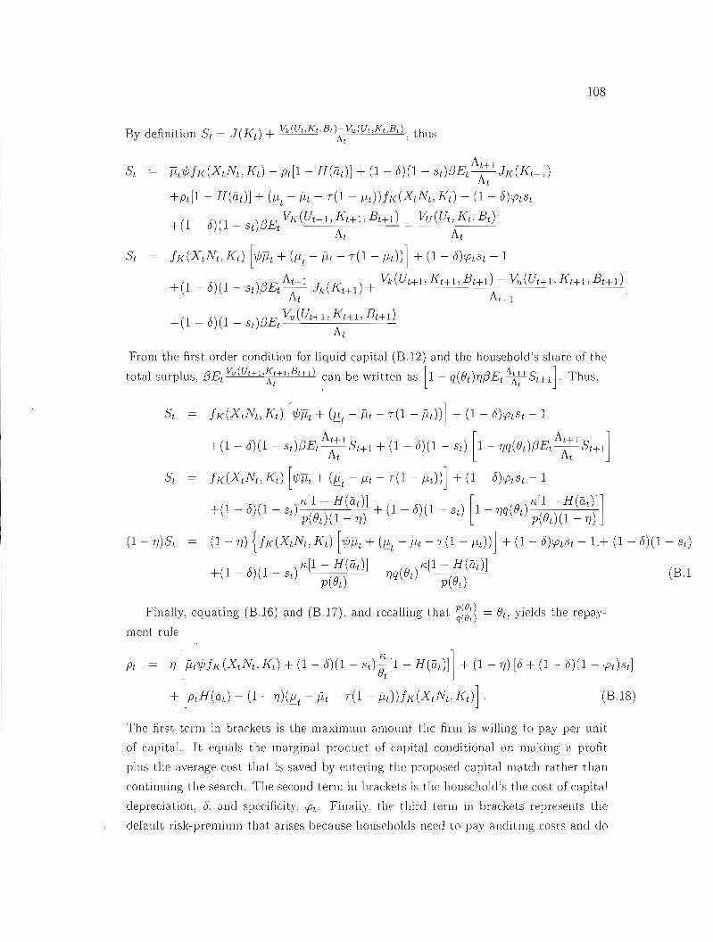
108
't' 5 - J(K) + Vk(Ut,Kt.Bt}-V,,(Ut,Kt,Bt) thBy defini IOn t - . t I\t : us
A St = Jit7/JfK(XtNt ,Kt} - pd1 - H(iit}] + (1 - 0)(1 - st}(3Et ~~l JK(Kt+J)
+pd1 - H(iit}] + (!:!.t - Pt - 7(1 - pt})fJ«XtNt, Kt} + (1 - o)<ptSt
+(1- 0)(1- st)(3E VidUt+l,Kt+l:Bt+l) _ Vu(Ut,Kt,Bt}t At At
St = .fK(XtNt:Kt} [7/J/lt + (!:!.t - Pt - 7(1 - Pd)] + (1 - o)<pt St- l
+(1 _ 0)(1- st)(3Et AHl [JdKt+d + Vk(Ut+1 : KHI: Bt+1 ) - Vu(Ut+!: K t+1l Bt+d] At A/Il
+(1 - 0)(1 _ sd(3Et Vu (Ut +1 : Kt+1l Bt+d At
From the first order condition for liquid capital (B.12) and the household's share of the
total surplus (3E V,,(Ut+l,Kt+i,Bt+J) can be written as [1 - q(B )'Yl(3E 1\1+15 ] Thus,t I\t' t '/ t 1\/ t+1· ,
St = fK(XtNt:Kt} [7/J/lt + (!:!.t - Pt - 7(1 - Pt))] + (1 - O)<ptSt - 1
At+1 - [ At+J]+(1- 0)(1 - sd/3Et-----;:::SHI + (1- 0)(1 - sd 1 - 7Jq(Bd(3Et -----;:::St+J
St fIdXtNt,Kt) [7/J/lt + (!:!.t - Pt - 7(1 - Pt))] + (1 - O)<PtSI. - 1
K;[1 - H(iit}] _ [ K;[1 - H(iit}]]+(1 - 0)(1 - St) p(B )(1- TJ) + (1 - 0)(1 - st} 1 - TJq(Bt ) p(B )(l - TJ)
t t
(1- TJ)St (1 - TJ) {fK(XtNt, Kt} [7/J/lt + (!:!.t - Pt - 7(1 - iLt))] + (1- o)<ptSt -1.+ (1 - 0)(1- st}
_ 5:)( _ ) K;[1 - H(iit )] _ (B) K;[1 - H(iit)] ((+ 1 u 1 St p(B ) rlq 1. p(B ) B.1t t
Finally: equating (B16) and (B.17), and recalling that ~~::\ = B,: yields the repay
ment rule
Pt = TJ [Pt7/J.fK(XtNt:Kt) + (1 - 0)(1 - st};; [1 - H(a tJ ]] + (1 - TJ) [0 + (1 - 0)(1 - 'Pt}stl
+ [PtH(iitJ - (1 - TJ)(!:!.t - ilt - 7(1 - Pt,)).fJ«(X,Nt:Kt)] . (B.18)
The first tenn in brackets is the maximum amount the finn is willing to pay per unit
of capital. It equals the marginal product of c8pital conditional on l1Iakillg a profit
plus the average cost that is saved by entering the proposed capital match rather than
continuing the sem·ch. The second term in brackets is the household:s the cost of capital
depreciation, O. and spccificity, 'Pt. Finally. thE' third term in brackets represents the
default risk-premium that arises bccause households necd to pay auditing costs and do

109
not receive the full contractual payment Pt when the nrm's idiosyncratic shock drops
belO\v at (zero profi t).
The Nash bargaining approach to determine the rentaI rate conditional on an op
timal separation threshold QL differs from existing financial accelerator models such as
Carlstrom and Fuerst (1997) or Bernanke, Gertler and Gilchrist (1998) where the priee
of capital and the separation threshold are chosen under the assumption that lenders
make zero profit. In our framework, this assumption would obtain for the special case
7) = O.
B.l.5 Aggregation and equilibrium
The micro literature on finn dynamics usually assumes decreasing returns to scale pro
duction (see for example Cooley and Quadrini, 2001 or Esteban-Rossi and Wright, 2005).
Bere, for reasons of tractability, we follow the traditional macro literature and assume
that the production function f(·) exhibits constant returns to scale. Uncler this as
sumption, it is straightforward to show that the capital labor ratio of ail firms is the
same. Bence, ail optimality conditions are independent of finn size and the rentaI rate
is identical for ail firms.
The constant returns assumption justifies our derivation of the optilllality conditions
in a representative firm framework, but at the same time bypasses any issues that arise
from finn size heterogeneity. These issues me adll1ittedly important but taking them
into account would rendel' our model less tractable and complicate the quantitative
analysis. In particular, we would no longer be able to draw direct comparisons with other
representative agent 1l10dels such as the frictionless RBC benc:hmark or the financial
accelerator model of Bernanke, Gertler and Gilchrist (1998).
A second simplifying assumption to keep our model tractable is the existence of a
state contingent insurance that covers for any shortfall in wage payments and costs of
project postings left over by béll1krupt firms (firms with productivity below QI for which
the household refuses to inject funds to continue the lending relationship). We assume
that this insurance is financed by the profits of firrns with productivity above aL. The remainder of the profi ts is transferred a t the end of each period to the household
in the fOfln of dividends. Bence, we a]:;o bypass any net worth conside1'8tions that are
at the center of the financial accelerator models of credit market frictions Aggregating

110
over the different firms, the total amount of dividends is defined as
Dt = 1~ [af(XtNL, Kt) - PtKt - WtNL- KYi] dH(a) (B.19)
Qt
+1 [af(XtNt , Kt) - WLNt - '"'Yi] dH(a).
The equilibrium of this economy is defined by the capital accumulation equation
(B.l), aggregate production J; af(XtNt , KddH(a) = f(XLNL, Kt) and the system of
equations (B.3)-(B.19).
In addition, by defining new capital investments as Ir ew = LL - UL- (1 - r5)VJLSLKt,
a familial' aggregate resource constraint can be derived:
where 7(1 - {lt) is the resource cost of monitoring, and KVt that of project postings.
B.2 Proof of Proposition 1
Proof: Consider the first order condition for liquid capital (13.12) in the presence of
exogenous capital separation only. Combined with the firrns' optimality condition for
project postings and the Nash bargaining results regarding the division of the match
surplus, this may be rewritten as At = (3Et At+1 + -2r,';;A t . By rearranging tenns;
congestion in the physical capital market can be expressed, in log deviations around the
steady state, as increasing function of the expected growth rate of the marginal utility
of consumption:
B.3 Equilibrium system
After normalizing by the deterministic trend to the la bol' augmenting technological
growth; the equilibrium systern comprises 22 equations for the variables Yt, Ct: nt; kt: li: lit:
Vt:Bt:p(Bt):q(Bt), rt,PI,wt:Àt:R~,dt,st,at.gL:{lt'!:!.t' Yt· where a lower case variable is

111
defined as Yt == ~.
Ct
w(1 - nt)-Ç = ÀtWt
Àt+1 TI t<;,Àt = fJEt - + ---[1 - H(at)]Àt9 1 - TI Bt
Àt = fJEt -Àt+1 [1 +rd
D
[1 - H(at)]wt = Ji (1 - o}t/J Yt t nt
t<;,[l - H(adJ t 1 = fJEt Àt~l {Jit+J'ljJa Y + - Pt+1 [1 - H(at+d] + (1- 0)(1 - St+1)t<;,[1 -(:(a;+d] lJ
p(Bd gAt kt+l P t+1 _ Yt . t<;,[1 - H(at )]]
Pt = TI {tt'lj;a kt + (1 - 0)(1 - sd B + (1 - TI) [0 + (1 - 0)(1 - it'dstl[ t
Yt+ [ptH(ad - (1 - TI)({t - Mt - T(l - Mt))a ]-t kt
gkL+J = (1 - 0)(1 - sdkt + q(Bdlt
Yt [1 - T(1 - Md] = Ct + [lt + Vtt<;,] - [(1 - O)Stit'tkt + îtt]
g1f,t+1 = [1 - q(Bd]lt
F4k = ptkt [1 - H(at)] + (I::: t - Mt - T(l - Md)Yt - (Wtnt + Vtt<;,) [H(at) - H(Qt)]
Rkdt + t Yt [1 - T( 1 - I:::t)] - Wtnt - Vtt<;, + (1 - O)it'tSsJ(t
ltBt =
Vt 1- fp(Bt ) B== t
q(Be) = B- f t
1-akQYt = A nt·t t
St = H(at) + SI
at = (Wtnt + Ptkt + Vtt<;,)/Yt
QtYt = Wtnt + Vtt<;, + (1 - o)kt {it't - (~) [1 - ~Et Àt;1 (1 - q(Bd)]} q l 9 9 t
it't = ç(sn
Ji t = ~oo adH(a)Jal
= ~t .~~ adH(a)
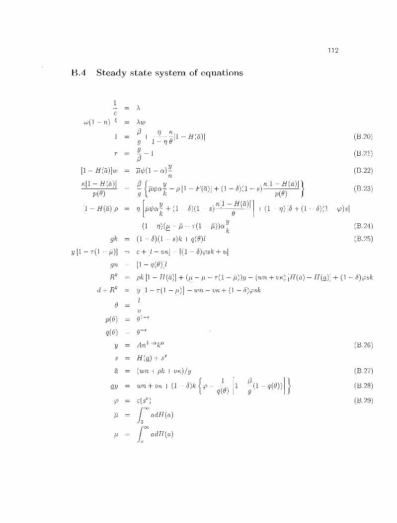
1
112
B.4 Steady state system of equations
À c
w(1 - n)-Ç Àw
13 TJ "" 1 9 + 1 - TJ e[1 - H(a)] (B.2ü)
9 T = --1 (B.21 )
13 [1 - H(a)]w Ji7/J(1 - ex) l!- (B.22)
n ",,[1 - H(a)] Q{Ji7/J ex '!l - p [1 - F(a)] + (1 - 0)(1 _ s) ",,[1 - H(a)] } (B.23)
p(e) 9 k p(e)
[1 - H(a)]p TJ [P7/Jex'!l + (1 - 0)(1 - s) ",,[1 - H(a)]] + (1 - TJ) [0 + (1 - 15)(1 - cp)s]k e
-(1 - TJ)(J.L - P - 7(1 - P))ex'!l (B.24)- k
gk = (1 - 6)(1 - s)k + q(e)l (B.25)
y [1 - 7(1 - p)] c + [1 + v",,] - [(1 - r5)cpsk + Hl
[1 - q(e)]l
pk [1 - H(a)] + (I!:- - P - 7(1 - p))y - (wn + v",,) [H(a) - H(g)] + (1 - r5)cpsk
= y[I-7(1-l:)]-wn-v",,+(I-r5)ysk 1e v
Ep(e) e1
q(e) e- E
y (B.26)
s H(g) + SI
a (wn + pk + vrv)/y (B.27)
gy wn + V"" + (1 - r5)k {cp - qte) [1 - ~(1 - q(e))]} (B.28)
cp = ç(SC) (B.29) 00
Ji adH(a)1I!:- .loc adH(a)

113
B.5 Computing the steady state
Using (B.20), (B.21) and (B.23), the equation for the repayment in the steady state can
be written as
1 - q) {f3 } _ _ y _p = (r+8)+ - r - (1 - - )(1 - 8)(1 - s) +(l-8)(1-cp)s-(tf-tf-T(l-tf))a:-+pH(a)( q.9 - k
Now, use (B.27) and(B.28) to form (a-gJ = [p-(1-8)\[r]~, from which t = [p-g~~t'l,
where \[r = {cp - qlo) [1 - ~ (1 - q(0))] }. The repayment is then
p (r + 0) + C~ q) {r - (1 - ~) (1 - 8) (1 - s) } + (1 - 8) (1 - cp) s
-(f!:. - ïi - T(l - ïi))a: [p -[;l_- f)\[r] + pH(a). g
Equation (B.23) defines the ratio of capital to output as
k ~a:
y [q(O)O (~- (1- 8)(1 - s)) + p[l- H(a)]]·
using first equation (B.20) to determine the value ~ = ~ (1 - ~). Since E(a) = 2a
1, the mean of the lognormal distribution is - IO~(Q). For a given ()~og(a) the cutoff
threshold g is given by g= H-1(se), where se is the proportion of separations occurring
endogenously. Given a value of H(a) one obtains values for p and ~. The nUll1erical
strategy is then to iterate over values of H(a) such that the equation relating the two
thresholds, (a - g) = [p - (1 - 6)\[r]~, is respected.
Using the production function the steady state capital stock is then simply
1
k = (1k) (.-=i n.
Equations (B26) and (B.22) give us the level of output and steady state wage. Liquid
capital is then computed using the law of motion of capital (B.25)
k[g - (1 - 8)(1 - s)] 1= q(O) ,
and unmatched liquid capital is 11 = (1 - q(O))~. Now both (B20) and (B.27) each
imply a value for vr{. \Ve thus iterate over values of () such that these two correspond.

114
Finally, the elasticity of separations to the cutoff {I, \}i, is given as
and the steady state values for profits, consumption, the Lagrange multiplier, and the
weight w are pinned down by the remaining steady state equations. The elasticity of the
loss of capital value to changes in the eut-off idiosyncratic productivity, f, is chosen to
match the relative standard deviation of the rate of capital separations due to financial
distress observed in the data.

115
B.6 Log-Linear system
êt = -Àt 1 - n '
nt = ~-[Àt + wtl çn
~Ed:\t+l] = ~:\t + (12 TJ) ~ [[1 - H(ii)]êt + iif(ii)at]
Et:\Hl + ~(rt - r) = :\t 9
~ ~ ~:::: iif(ii) ~ Wt = Yt - nt + f.1t + [1 _ H(a)]w at
gkkH1 = (1 - 0)(1 - s)kkt - (1 - o)skSt +lq(B) [~+ q(êJ] ~ ~ q(B)--
gUt+l = lt - 1 _ q(e) q(et )
y [1 - T(1 - il,)] Yt = cêt + l4 + 7JK.Vt - (1 - o)si.pk [St + kt + tPt] - UÛt + TYl-t~t
ddt + RkRf- = Y [1 - T(1 -,ü)] Yt - wn[Wt + nt] - VK.Vt - TYf.1~t + (1 - o)si.pk [St +kt + tPt]
iiy(at + Yt) = k(pt - p) + pkkt + wn(Wt + nt) + VK.Vt
Yt = Ât + (1 - o)n,t + okt
êt = lt - Vt
p(èJ = (1 - é)êt
q(èJ = -éêt sa ~
St = -Sat S
$àt = i.p~t
tPt = [Qt
f.1M = _g2 h(Q)Qt
f.1~t = -a?h(a)~t
~ --- iif(ii):::: ~ Àt - p(Bd - [1 _ H(a)] at = EtÀt+1
f3 p(e) p;ljJoy [~ ~ ::::] K. ~ +"9 -;- { [1 - H(a)] k YHl - kt+J + f.1t+l - (Pt+l - p) - (1 - o)s p(e) SHI
( ")' ) K. ----(fJ) [ ( ")( ) K. iif(ii)] :::: }- 1 - 6 II - s p(B)P 0t+J + P - 1 - 6 1 - S p(e) [1 _ H(a)] at+l

116
[1 - H(a)J (Pt - p) = (X~ ('fl'ljJJi - (1 - 'fl)(J.1- jj - T(1- jj))) [Yi - kt]k 11,[1 - H(a)] ] ~ 11,[1- H(a)]~
- 'fl(1 - 6) B - (1 - 'fl)(1 - 6)(1 - <p) SSt - 'fl(1 - 6)(1 - s) B Bt[
- [p - 'fl(1 - 6)~] ah(a)Z1t + (X~ ['fl'ljJ - (1 - 'fl)(1 - T)] {LMt - (1 - 'fl)(1 - T)(X~J.1fJt
-(1 - 'fl)(1 - 6)'!Js'Pt
Rk R~ = k[1 - H(a)](pt - p) + pk[1 - H(a)]kt + Y(~ - jj - T(1 - jj))Yt + YJ.1fJt - (1 - T)Y{LMt
-wn(H(a) - H(g))[Wt + ?id - vK,(H(a) - H(g))Vt - [wn + pk + vK,Jah(a)Zl:t + [wn + VK,Jgh(g)Çit
+(1 - 6)s<pk [St + kt + 'Pt]
gy(Çit + Yt) - wn(Wt + nt) - VK,'Ût = {(1 - 6)k ['!J - qtB) [1 - f(1- q(B))]]} kt
(l-q(B))(3 ~ ~ (1-6)k( (32(3 )+(1 - <5)k q(B) 9[EtÀt+1 - Àt ] - q(B) 1 - 9+ gq(B) q(Bd
+(1 - <5)k<p'Pt
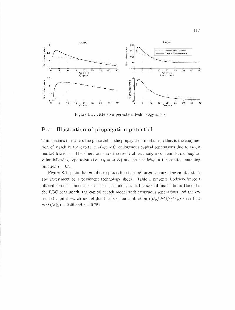
117
Output Hours 0.6
Nesled ABC model
'0 >- -- C<,pilal Search model ~ 0.4
ID '" 0.2Vi E g 0!':1 .,
'"
0.5 --~-~--':--='--~---:':=-----::'::-~ -0.2 o 5 10 15 20 25 30 35 40 0 5 10 15 20 25 30 35 40
Quarters Quarlers Capital Investment
ID
1.51 n; Vif4 Vi E 2 g if!.
0 '-J":r==:=6
o 5 10 15 20 25 30 35 40 0 5 10 15 20 25 30 35 40 Quarters Quaners
Figure B.l: IRFs to a persistent technology shock.
B.7 Illustration of propagation potential
This sections illustrates the potential of the propagation mechanism that is the conjunc
tion of search in the capital market with endogenous capital separations due to credit
market frictions. The simulations are the result of assuming a constant loss of capital
value following separation (i.e. 'Pt = zp Vt) and an elasticity in the capital matching
function E = 0.5.
Figure B.l plots the impulse response functions of output, hours; the capital stock
and investment to a persistent technology shock. Table 1 presents Hodrick-Prescott
filtercd second moments for this scenario along with the second moments for the data,
the RBC benchmark; the capital search model \vith exogenous separations and the ex
tenrip.d capital scareh mode1 :for the baseline calibration ((azp/fJc;e)/(se lep) sllch that
a(se)la(y) = 2.46 and E = 0.25)
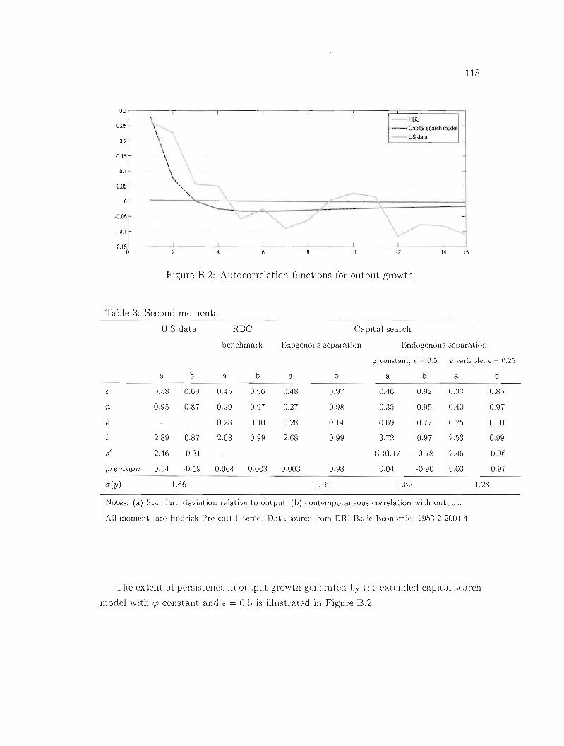
118
03i---,------,------,------,------,-----r======::::;1 --ABC - Capilal search model0.25
USdala 0.2
0.15
0.1
0.05
o
~:~ j _0.15'------'-- ----L '--_.__-'- ----L1 LI ----'__1
o 10 12 14 15
Figure B.2: Autocorrelation functions for output growth
Table 3: Second moments
D.S data RBC Capital search
benchmark Exogenous separation Endogenous separation
'P constant, € = 0.5 'P v~.riable, t = 0.25
a b a b a b a b a b
c 0.58 0.69 0.45 0.96 0.48 0.97 0.46 092 0.33 0.85
n 095 0.87 0.29 0.97 0.27 098 035 0.95 DAO 0.97
k 028 0.10 028 014 069 077 0.25 010
2.89 0.87 268 0.99 268 0.99 3.72 0.97 2.53 0.99
se 2.46 -0.31 121O.J7 -0.78 2.46 -0.96
premium 0.54 -0.59 0.004 0.003 0.003 0.98 0.04 -0.90 0.03 -0.97
a(y) 1.66 J.l6 1.52 128
Notes: (a) Standard devialion relative tu output; (b) conlemporaneous correlation \Vith output.
Ail moments are Hodriek-Prescott fjltered. Data source [rom DRI Basic Economies 1953:2-2001:1
The extent of persistence in output growth generatecl by the cxtencled capital search
model with :p constant and E = 0.5 is illustrated in Figure B.2.

119
B.8 Data sources
Ali time series used in this paper are quarterly data taken from the DRI Basic Economies
database (formerly Citibase) We restrict our statistical analysis to the sample 1953:2
2001:4. Data related to firm-level property, plant and equipment are from Standard and
Poor's Compustat database, for the period spanning 1980-1993. Finally, bankruptcy
filing data are from the Bankruptcy Research Database compiled by Prof. Lyn LoPucki
at DCLA's law department. This covers filings by publicly traded firms in the D.S.
since October 1979. The following table gives the definition and a short description of
the different series (where the definition is given in actual DRJ mnemonics)

Table 4: Data description
Compustat
variable data item
Property, plant and equipment, gross 7
Property, plant and equipment, net 8
Sales 107
Retirements 184
H,eason for deletioll aftnt35
Year of deletioll aftnt34
DRI Basic Economies datahase
Variable Definition Description
7J In(gdpq-gpbfq)-ln(pI6) real GDP (non-farrn) pel' eapita
c In(gcnqTgcsq)-ln(pI6) real pel' eapita private eonsumption of non-durables and servies
ln (gifq)-ln( p16) real pel' eapita private fixed investment (ine!, residential)
n In(lpmhu)-ln(pHi) total hours (non-farm) pel' eapita
>--' !'-)
o

Appendix C
Endogenous Flows of Foreign Direct
Investment and Interllational Real
Business Cycles
C.I Flows of FDI and Canada - D.S. business cycles
Table C.l: Data series and sources
Canada United States
source series source series
Output Statistics Canada \11992067 Fred Il : BE.A GOP96
Consumption Statistics CanaDa \11992044 Fred Il ·13.E.A PCESYC96+ PCNOGC96
Hours Statistics Canazla \13443721 Fred Il : B.L.S AWHl
!nvestment. Statistics CanaDa \11992051 Fred 11 BE.A PNFIC96
investment deftalor Statistics Canada Table 380-0003 Fred Il B.E.A
FDI in Canada* Statisl.ics Canada Table 376-0003
gross inAows \1113032
gross outftows \111:3035
Canadian Inv. abroad* Statistics CanaDa Table 376-0003
gross inAows v11302J
gross outAows v]]3018
*: Excludes portfolio investmenl Aows

122
Real GDP per capita
::~~.~~""'~:--:J;;~6i001 '-- ---'--- -'-- -----'- -L- '-- ----'--
1975 1980 1985 1990 1995 2000 2005 Hours
:::,-------f - - --,---"_-------,-------o' - - ~ : jo' ._---'-------: .'•• '--------,--"u---,--_
1975 1980 1985 1990 1995 2000 2005 x 10-3 real investment
6r--------.-----,--------,.----,-----r------r-...,
O'---------'------..l..---------'-- ..l- '-- ---L--'
1975 1980 1985 1990 1995 2000 2005 real consumption
:~t· .--.--,- ..-.---:-.-.---~ ---..-.~ -------:----.---j 1975 1980 1985 1990 1995 2000 2005
Figure Cl: Evolution of prominent macroeconomic variables, Canada and the US .. 1976-2005.
C.I.I Canadian and US macro variables.
Figure C.l shows the evolution of hours worked (indexed), real output, investment and
consumption per capita, over the period 1976-2006, for Canada and the U .S.. The
general observation is of a clmie similarity in per capita variables. \Vith fe\V episodes
where each country follows a different path. One example is the outpl1t pel capita gap
appearing during the 1990s, which also shows up as a gap in average hours worked.
C.I.2 Foreign controlled firms in Canada
The following table presents the share~ of assets and operating revenue of foreign con
trolled non-financial finns in Canada. j\ilanufacturing stands out a~ a ~ector \Vith a
large share of emploYlllent and high degree of foreign controL involving nearly one fifth
of employment and where j ust over half of the revel1ue~ and a~sets are under foreign
controL

123
Ope là'Ig fe\'!!rtJ.. AS~~15
5!>.~ 'Il 121 'i1.7 50. 1 t 1 .!t7 .\1.G L ••7141 36,6 33." 13. • 1
11 6.3 (1 • .15 .. 00 ':1.mn :J ','iâl'E' ;'C.!> l'il ~.8
Adn ~ arrl ~ wa5tE>m <nar:;p;:rn€l'ltirlCl JIlInedBti:n Belv:œ.s 19,4 23,5 ~) 6,Q2 RetaJ1moœ 162 21 (7) 15,68 P JOB&Ùr"-l scmtfr m~llli:e9 15.3 15.5 ~} 6,26 Re-A1eard.1Hlta1.ar:d Ss:i:q 11,7 1J.8 (ll) 2,24 Acr:nn m oœti:n ax.I iJod sell7:ŒS 10,5 14,7 1,10) 8,95 :hilm ati:n m OIb=lixhstù;>s 9-:' 6,5~} J,TI Repli; ma:iIIere:nce andpeœm.a1Bel.Vi:Es 6;5 1.8,4 fl) 4,51 Ca'l5tltldin 4,5 4.7 (1.4) 6,25 EcUcaâlraJ,bealln.-œ IIndaoo-j1lass};t;nœ sellli:es 2..l 1,5 (l.7) 9,D4 AIl5,erœlla:i:rn entard recŒli1ltin 1,8 2,2 (1.5) 2,35 Agri:l.ùuJe , D:SIy.. fi:h:r.g ard h:.1rt:bg 1,7 1,7 (16) 0,62
Tolal no nnanclal imluqlri&$ 30,7 28.5 100
Soorœ;Slatiitics C-anaœ noll'!S. • incJudl>, mi ning.
Figure C.2: Share of operating revenues and assets under foreign control - non-financial incl ustries 2004
C.2 Models
This section presents the full cletails of the three models simulated in the paper.
C.2.1 IRBC with search in FDI, endogenous reallocation and
investment adjustment costs
Each country is populated by dornestic and foreign firms and a representative hOl1sehold.
HOl1seholds decide On optimal consumption, an aggregate of goods prodl1ced by both
types of firms. and allocation of investment goods to firms located at hOIlle or abroad
Initiating a new investment project abroad required disbursing a flow cost l'ô. and is
subject to a time consuming search and matching process. No such friction applies
to changing production capacity at home. Thus domestic firms rent capital on spot
markets while foreign firms chose the amount of new projects to initiate. As will be
scen lateL the frictionless ca.pital market is a special case of the search environment
with K. = O. Firms, domcstic and foreign, hire labor on competitive domestic markets.
Finally, clomestic and foreign firms prodl1ce interrnecliate goods aggregatecl into a final
homogeneous consulllption good by an Armington (1996) a.ggrega tOI' Yt = G (Yf, y{di) = 1
[<b(Yft + (1 - rjJ)(y{di)v];;-, \Vith elasticity of substitution '1/; = 1/(1 - v) and relative

124
shan~s determined by the parameter 4>. The relative priee of the foreign firm's good is
thensimplyp{di = C2 (yf,y{di) and thatofthedomesticfirm'sgoodPf = Cl (yt,y{di).
C.2.1.1 Domestic and foreign producers
Domestic firms produce with technology yf = At(nf)I-D:(kf)D:. Optimization yields the
following two first order conditions:
pdVdwf = (1- o)~dn t d d
r d = o,Pt Yt t d .
kt
The following is the dynamic problem for foreign firms:
, [fdiA ( fdi)l-D:(kfdi)D: _ fdi fdi _ .fdikfdi _ + (JE À~+l J(k.fdi )]!J1d'fC Pt t nt t w t nt Tt t KVt t À* t+l
ni ,VI t
b· kfdi*su Ject to Hl (1 - 0)(1 - St)k{di + p(BI)Vt
Optimization yields the following two first order conditions:
(n{di)
(VI) :
fdiwhere Jkfd,(kt+l) IS the marginal value of an additional unit of capital to the fi fi11 ,
defined as
f~ f~ À* J '(kfdi)_ Pt Yt .fdi (')( )6E t+lJ '(k fdi )kfd' t+1 - 0 fd' - Tt + 1 - u 1 - St+!, 1 ~ kfd, 1
ktt /\7
In cornbination with the first order condition for project initiations, this yield the forward
looking condition
\ * { fdi fdi }K _ /\1+1 Pt Yt+ l fdi K-(8) - {3Ety 0 jdi - r l+1 + (1- 0)(1- St) (0 ) . Ptt kt+! P I+!
C.2.1.2 Domestic households
Households choose a level of aggrega te consumptiOll (defined as the Sllm of both inter
mediate goods). hours to supply to both domestic and foreign employers, and have two
capital investlllcnt options: illvesting in firms Clt home or investing in capacity abroad.

125
In addition, there are convex cost to new investments: domestic and foreign. The
resulting dynamic program for the representative household is thus
V(kt, k{di*, un = max [U(Ct> 1 - nd + (JEt V(kf+l: k{~~*, U;+l)]nf,n{ dl ;i t , Jdi;
subject to wfnf + w{din{di + rfkf + r{di*k{di* + n; = Ct + qfi1 + q{düi{di*
and k[:~* = (1 - 8)(1- sdk{di + q(e;)l;
~ d fdid - kd (1 ')kd d d d fdi* " . 1 hwhere nt - nt + nt ,It - Hl - - Ut' an qt an qt arc, JespectJve y, t e
cost of new investment goods destined for plants at home and abroad. This cost is
given by qt = [<p' (ft)rI, with <p' (.) > °and <p" (.) < 0, and such that in the steady
state q = 1. New investment goods destined for foreign direct investrnent are defined as
i{di. = l;-(1-o)St k{di* -u;, where (1-0)stk{di* is capital recuperated from terminated
operations abroad, net of depreciation, and Ut are units of investments goods not yet
allocated. Thus l; is the total amount of investment goods available for allocation to
production abroad.
The optimality conditions are
(Ct) uc(c(,l - nt) = Àt
(nf) Und(Ct: 1 - nd = Àtwf
(n{d') Unfdi(Ct, 1 - nt) = ÀtWtfdi
(k'dH 1) Àtqf = (JEt [rf+l + qf+l(l - 0)]
\ fdi* _ {JE [(e*)17 . (k d k.fdi* * ) (1 (e*))V (k d ,jdi* * )]/\tqt - t q t vkf d'" Hl: t+J 'Ut+l + -q t u t+l,I>-{+l :Ut+l
where the marginal values of allocated and non-allocated investment goods are
The repayment on capital is detennined by Nash bargaining over a surplus defined as

126
. V (k d• k!di ) V (kd' k!di )- J(k.Jd~) k!di t ,t ,Ut - " t ' t,Ut •St - t + >" . t
V (kd' k!di ud fdi >'"The first order condition on lt can be rewritten as f3Et 'li t ~.t' = qt -7)q(Bdf3Et ~: 1 St+1
t t
such that
p{diy{di fdi [( ") J] ( ')( )f3E À;+1 S' a k{di + qt 1 - U St - . + 1 - () 1 - St t ÀZ t+ 1
+(1 - 6)(1 - sd [q{di - 7)q(Bt )f3Et ÀI;1 St+1]
fdi fdi Pt Yt f di [() () )] ( ') ( ) Ka fd + qt 1 - 6 St - 1 + 1 - 6 (1 - St + 1 - 6 1 - St (B)( )
kt l P t 1 - 7)
-(1 - 6)(1 - St)-7)- ~ 1-7)Bt
fdi fdi Pt Yt fdi s: ( ') ( ) K
St = a fdi + qt U + 1 - () 1 - St (B) ( )kt P t 1 - 7)
- ( 1 - () 1 - St -- ') ( ) 7) K
1-7)Bt
From the definition of J(k{di) we have
fdi fdi _ Pt Yt f di ). ri,
(1 - 7) )St - a k fdi - Tt + (1 - 6 (1 - St) p(B )tt
Cornbining these two yields
f~ f~ . fdi _ Pt Yt ( ) fdi, ( ) ) KTt - J]a fdi + 1 - 7) qt () + 7) 1 - 6 (1 -.5 e
kt 1
C.2.1.3 Endogenous reallocation
\Ve assume the existence of a randOlll idiosYllcratic productivity to the match: the real
ization of which occurs aftel' production decision are made aud factor price equilibria are
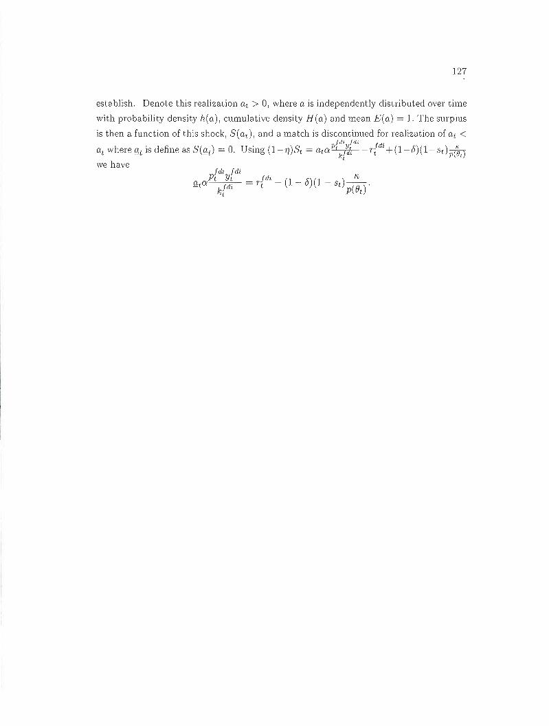
127
establish. Denote this realization at > 0, where ais independently distributed over time
with probability density h(a), cumulative density H(a) and mean E(a) = 1. The surplus
is then a function of this shock, S(ad, and a match is discontinued for realization of at < fdi fdi f'
Qt where Qt is define as S(QJ = O. Using (l-7])St = atCiPtkf~~ -Tt dt+(1-e5)(1-8dp(~tl
we have /'

128
C.2.1.4 Equilibrium system of equations
7.ic (Ct; 1 - nd Und (Ct; 1 - nd
'Unfd, (Ct; 1 - nd Àtqf
\ fdi* Atqt
·d2t
-fdi* 2t
k fdi * t+l
y1 Ytf d
l
B
p(Bd
q(Bd
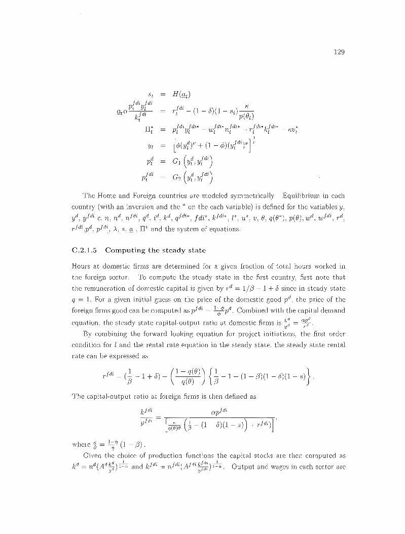
129
Yt
fdi Pt
The Home and Foreign countries are modeled symmetrically Equilibrium in each
country (with an inversion and the * on the each variable) is defined for the variables y,
yd; yfdi c, n; n d; n fdi , qd, id; kd; qfdi*, fdi*, k fdi *, Z'; u*; v; B, q(B*), p(B),wd, Wfdi ; rd;
rfdi,pd, pfdI ; À, 5, Q. , D* and the system of equations.
C.2.1.5 Computing the steady state
Hours at domestic firms are determined for a givcn fraction of total hours workcd in
the foreign sector. To compute the steady state in the first country, first note that
the remuneration of domestic capital is given by rd = 1/f3 - 1 + 6 since in steady state
q = 1. For a given initial guess on the priee of the domestic good pd, the price of the
foreign firms good can be computed as pfdi = l;<1>pd Combined with the capital demand
equation, the steady state capital-output ratio at domestic firms is ~: = ~~d.
By combining the forward looking equation for project initiations, the firsL order
condition for Z and the renta} rate equation in the steady state. the steady state renta}
rate can be expressed as
fdir = (2. -1 + 6) + (1- q(B)) {2. - 1- (1- (3)(1 - 6)(1 - 5)}f3 q(B) f3 . .
The capital-output ratio at foreign firms is then defined as
kfdi Ctpfd'i
di yf [q(ê)B 0- (1-6)(1-s)) +rfdi )]'
where ~ = 1 ~'7 (1 - (3) .
Given the choice of production functions the capital stocks are the]} computed as
kd = nd(Adk:) l~o and kfdi = n/di(Afdi kIl::) l~Q. Output and wages in each sector are y y

130
then given by their respective equations and the share parameter 1J is chosen such that
wd = wfdi is satisfied.
Investment in domestic firms is given by id = 8kd To compute new investment
goods i fdi , first compute l as l = k!J-(lq(~i(l-S)1 and u = (1 - q(B))l. Then i fdi = l - (1 - 8)sk fdi - u.
The variance of the idiosyncratic shock is computed numerically to satisfy the eut-off j di jdi fd'
value definition; gaP kj~i = rl
- (1 - 8)(1 - s)p~)' and that for the separation rate,
s = H(QJ
The same procedures obtain the corresponding steady state values for the foreign
country,
Finally; consumption is obtained using the budget constraint and À by using the first
order condition on consumption.

131
C.2.2 IRBC with FDI and investment adjustment costs
C.2.2.1 Domestic and foreign producers
As before, domestic and foreign finns produce intermediate goods aggregated into a final
homogeneous consumption good by an Armington (1996) aggregator Yt = C (yf, y{di) = 1
[<f;(y1)V + (1- </J)(y{di)v];, \Vith elasticity of substitution 't/J = 1/(1 - li) and rela
tive shares determined by the parameter </J. The relative priee of the foreign firm's
good is then simply p{di = C2 (yf, y{di) and that of the dornestic firm's good pf =
Cl (yr, y[di) .Dornestic firms face the same problem as above. When there is no search
cost, firms post an infinity of projects and ail capital is reallocated in the beginning of
each period; i.e. s = 1, q(()t) = 1 and 'Ut = O. Thus the foreign firm problem is now
static. Optimization yields the following two first order conditions:
Jdi Jdi ( Jdi) Jdi _ (1 _ )Pt Ytnt wt - 0: Jrh
nt Jdi Jdi
.Jdi _ Pt Yt r t - 0: Jdi
kt
C.2.2.2 Domestic households
The household's dynamic prograrn is now1
.Jdi* kJdi * (1 5:)k Jdi * Th . l' d' .Note that now %t = 't+l - - U "t '. e optima Ity con ItlOns are
(Ct) 1ic(Ct, 1 - nt) = Àt
(nt) Und (ct: 1 - nt) = Àtwt . _ Jdi(n{di) Ullfd" (Ct: 1 - nt) - ÀtWt
(kt+l) Àtqf = ,BEt [r1+1 + qt+l (1- 0)]
(kJd'i* ) À fdi* - {JE [.J di* + f di *(1 - 8)]t+l tqt - t T t+1 qt+l
C.2.2.3 Equilibrium system of equations
The hOllle and foreign countries are Illodeled symmetrically. Equilibriulll in eacb country
(with an inversion and the * on the each variable) is clefined for the variables Y: yd, yJdi c,
J Note Chai taxes on capital fiows have been omit.ted.

132
n, nd, n idi , qd: id, k d, qidi*, Jdi*, k idi*, wd, widi , rd, r idi , pd, pidi , À and the system of
equations,
Uc(Ct, 1 - nd À t
Und (ct, 1 - nt) Àtwr
idi lln i di (Ct; 1 - nt) ÀtWt
Àtqf /3Et [rt+1 + q1+1(1 - 0)]
/3Et [r{~~* + q{:~* (1 - 8)] d iJ>1 (4 )] -]
qt k1[
<1>1 ( Jdi~ )] -] [ kidl' t
k1+ 1 - (1 - 8)kt kfdi * _ (1 _ 6)edi*
t+l t d d
(1_Q)PtYtdn t
d d + idi idi + dkd + idi*kidi*W t nt wt nt rt 1 r t t
d Yt idi
Yt
1
[<1>(y1r + (1 - <j;)(y{di r ];; cl id;)G1 (Yt ,Y,
id; i di )dPt G. 2 (YI.: YI.

133
C.2.2.4 Computing the steady state
The procedure is identical to previously with the exception that now the remuneration
of domestic and foreign capital are given by rd = 1/f3 - 1 + 6 and r fdi = 1/f3 - 1 + 6,
since in the steady state q = 1(the second rentai rate uses the foreign household's first
order condi tion on foreign investment).
C.2.3 IRBC with search in FDI, exogenous separations and
investment adjustment costs
The problem faced by domestic and foreign firms, and households, is the same as in the
endogenous separation case. Computing the steady state involves the same procedures,
save the iteration to pin down the varia.nce of the idiosyncrat.ic shock.

Bibliography
[1] Abraham, Katherine G. and John C. Haltiwanger (1995). "Real Wages and the
Business Cycle," Jo'u.rnal of Economie Literat'Ure vol. 33(3), pp. 1215-1264.
[2] Acemoglu, Daron, (2001). "Credit Market Imperfections and Persistent Unem
ployment," Ev,ropean Economie Review, Papers and Proceedings. vol. 45(4-6), pp.
665-679
[31 Ambler, Steve, Cardia, Emanuela and Christian Zimmermann (2002). "Illterna
tional transmission of the business cycle in a multi-sector model," E'UTOpean Eco
nomie Review vol. 46(2), pp. 273-300.
[4] Ambler, Steve, Cardia, Emanuela and Christian Zimmermann (2004). "Interna
tional business cycles: What are the facts?, " Journal of Monetary Economies vol.
51(2), pp. 257-276.
[51 Andolfatto, David (1996). "Business Cycles and Labor-IVlarket Search" , American
Economie Review vol. 86(1), pp. 112-132.
16] Andolfatto, David and Glenn IvIacDomdd (2006). "Jobless Recoveries", working
paper.
17] Backus, David K., Kehoe, Patrick J. and Finn E. Kydland (1992). "International
Real Business Cycles," The Journal of Politieal Eeonomy vol. 100(4), pp.745-775.
[8] Backus, David K., Kehoe, Patrick J. and Finn E. Kydlalld (}Cl95). "International
Real Business Cycles: Theory and Evidence." ln: Cooley, TF (Ed.). Frontiers of
Business Cycle Reseal'ch. Princeton University Press. Princeton. ~J. pp. 331-356.
[g] Baldwin, John R. and Gander DhaJiwal (2001). "Heterogcneity in Labour Pro
ductivity Growth in J'vlallufacturing;: Differences Between Domestic and Foreign
control!ed Establishments", Statistics Canada catalogue no. 15-204. Chapter 5.
134

135
[10] Baldwin, John R. and Guy Gellatly (2005). "Global Links: Long-Term Trends in
Foreign Investment and Foreign Control in Canada, 1960 to 2000," The Canadian
Economy in Transition 2005008e, Statistics Canada, IVlicro economic Studies and
Analysis Division.
Ill] Barron, John M., Berger, Mark C., and Dan A. Black (1997). "Employer Search,
Training, and Vacancy Duration," Economie Inquiry vol. 35(1), 167-92.
[12] Barran, John M., and John Bishop (1985), "Extensive Search, Intensive Search,
and Hiring Costs: New Evidence on Employer Hiring Activity," Economie Inquiry
vol. 23(3), pp. 363-82
113] Basu, Susanto and John G. Fernald (1997). "Returns to Scale in U.S. Production:
Estimates and Implications," Journal of Political Economy, vol. 105(2); pp. 249
283.
[14] Baxter, Marianne, and Mario J. Crucini (1995). "Business Cycles and the Assel
Structure of Foreign Tracle,1l International Economie Review, vol. 36(4), pp. 821
854.
115] Baxter; Marianne and Dorsey D. Fan (2005). "Variable capital utilization and
international business cycles, "Jo'urnal of International Economies; vol. 65(2). pp.
335-347.
[16] Becker, Randy, John Haltiwanger, Ron Jarrnin, Shawn Klimek and Dan Wilson
(2006). "Micro and Macro Data Integration: The Case of CapitaL" In: Dale W.
Jorgenson; J. Steven Landefeld; and \Nilliam D. Nordhaus (Eds.), A New Archi
tecture for the U.S. National Acco1J.nts, NBER. pp. 541 - 610
[17] Bernanke, Ben S. and Mark Gertler (1989). "Agency Costs. Net Worth and Busi
ness Fluctuations," American Economie Review vol. 79(2). pp. 210-214.
[18] Bernanke, Ben S.. Gertler, Mark and Simon Gilchrist (1999). "The Financial Ac
celerator in a Quantitative Business Cycle Framework" In: Handbook of Macroe
conomies, J.B. Taylor and NI. Woodford (eds.), eclition 1, volume 1, chapter 21,
pp. 1341-1393
[19] Blanchard; Olivier and Peter Diamond (1990). "The Cyclical Behavior of the Gross
Flows of U.S. \Norkers;" Brookings Papers on Economie Activity 2. pp. 85-] 55

136
[20J Blanchard, Olivier and Nobllhiro Kiyotaki (1987). "Monopolistic Competition and
the Effects of Aggregate Demand," American Economie Review, vol. 77(4), pp.
647-666.
[21J Blinder Alan. S. and Louis. J. 1'vlaccini (1991). "Taking stock: a critical assessment
of recent research on inventories;" Journal of Economie Perspectives, vol 5(1),
pp.73-96.
[22J Boileau, Martin (1999). "Trade in capital goods and the volatility of net exports
and the terms of trade," Journal of International Economies, vol 48(2), pp. 347
365.
[23] Boldrin, Michele, Lawrence J. Christiano and Jonas D. M Fisher (2001). "Habit
Persistence; Asset Returns, and the Business Cycle," Ameriean Economie Review,
vol. 91(1), pp. 149-166,
124J Brainard, S. Lael (1993). "An Empirical Assessment of the Factor Proportions
Explanation of Multinational Sales;" NBER working paper No. 4269
[25J Brainard, S. Lael (1997). "An Empirical Assessment of the Proximity
Concentration Trade-off Between Multinational Sales and Trade", Ameriean Eco
nomie Review vol. 87(4), pp. 520-544
\26J Brandolini, Andrea (1995). "In Search of a Stylised Fact: Do Real Wages Exhibit
a Consistent Pattern of Cyclical Variability?," Journal of Economie Surveys. vol
9(2); pp. 103-163
[27] Caballero, Ricardo, Eduardo Engel and John C. Haltiwanger (1995). "Plant-Level
Adjllstment and Aggregate Investment Dynamics," flrookings Papers on Eco
nomie Aetivity 2, pp. 1-39
128J Caballero, Ricardo J. and JVloharnad L. Hammour (1996). "The "Fundal1lental
Transfornwtiom in Macroeconomics;" American Economie Review. vol. 86(2); pp.
181-186
[291 Carlstrom, Charles T. and Timothy S. Fuerst (1997). "Agency Costs; Net Worth,
and Business Cycle Fluct uations: A Compu table General Eq uilibrium Analysis."
Ameriean Economie Review, vol. 87(5), pp. 893-910
[30] Carlstrom; Charles T. and Timothy S. Fuerst (2000). "j'vlonetary Shocks; Agency
Costs and Business Cycles." Federal Reserve Bank of Clevelanù working pCljJer
00-11

137
[31] Checchi, Daniele, Navaretti, G.B. and A. Turrini (2003). "Adjusting labour de
mand: multinational versus national firms - a cross-european analysis," Journal
of the European Economie Association, vol. 1(2-3), pp. 708-719
[32] Christensen, Ian and Ali Dib (2003). "Monetary Policy in an Estimated DSGE
Model with a Financial Accelerator," Bank of Canada working paper 03-27
133] Christiano, Larry, Eichenbaurn, Martin and Charles L. Evans (2005). "Nominal
Rigidities and the Dynamic Effects of a Shock to Monetary Policy," Journal of
Political Economy, vol. 113(1), pp. 1-45
[34] Cogley, Timothy and James M. Nason (1995). "Output Dynamics in Real
Business-Cycle Models," American Economie Review ,vol. 85(3), pp. 492-510
[35] Cooley, Thomas F., Ramon Marimon and Vincenzo Quadrini (2003). "Aggregate
consequences of limited contract enforceability," NBER working paper 10132
[36] Cooper, Russell, John C. Haltiwanger and Laura Power (1999). "Machine Replace
ment and the Business Cycle: Lumps and Bumps," Amer-ican Economie Review,
vol. 89, pp. 921-946
[37] Cooper, Russell, John C. Haltiwanger (2006). "On the Nature of Capital Adjust
ment Costs," Review of Economie Studies, vol. 73(3), pp. 611-633
[38] Covas, Francisco and Wouter den Haan (2006). "The Role of Debt and Equity
Financing over the Business Cycle, Il Bank of Canada working paper 06-45
[39] Crucini, l'dario J. (2008) "International Real Business Cycles. " ln: The New Pal
grave Dictionary of Economics; 2nd edition, Steven Durlauf and Lawrence Blume,
eds., Palgrave Macmillan Ltd:London
140] Davis, Steven .1., Jason Faberman and John Héllti\vanger (2006). "The Flow Ap
praach to Labor Markets: New Data Sources and Micro-Macro Links," Journal of
Economie Per-spectives, vol. 20(3). pp. 3-26
[41] Davis, Steven, John C. Haltiwanger, Ron Jarmin and Javier :Miranda (2006).
"Volatility and Dispersion in Business Grawth Rates: Publicly Traded versus Pri
vately Held Firms," NBER working paper 12354
1421 Den Haan, Wouter .1 .. Rame)'. Garey and Watson, Joel (2000). "Job Destruction
and Propagation of Shocks," American Economie Review. vol. 90(3). pp. 482-498

138
[43] Den Haan, Wouter J., Garey Ramey and Joel Watson (2003). "Liquidity Flows and
Fragility of Business Enterprises", Jourmal of Monetary Economies, vol. 20(3), pp.
1215-1241
[44] Diamond, Peter (1990). "Pairwise Credit in Search Equilibrium," The Quarterly
Journal of Economies, vol. 105(2), pp. 285-319
[45] Doms, Mark E. and Timothy Dunne (1998). "Capital Adjustment Patterns
Manufacturing Plants," Review of Economie Dynamics, vol. 1(2), pp. 409-429
111
146] Eisfeldt, Andrea and Adriano Rampini (2006), "Capital Reallocation and Liquid
ity." Journal of Monetary Economies} vol. 53(3), pp. 369-399
[47] Eisfeldt, Andrea and Adriano Rampini (2007), "New or Used: Investment with
Credit Constraints," Journal of Monetary Economies, vol. 54(8), pp. 2656-2681
[48] Elsby, Michael W. and Ryan Ivlichaels (2008). "Marginal Jobs, Heterogeneous
Firms, & Unernployment Flows," NBER Working Paper No. 13777
[49] Elsby, l'vlicheal W., Ryan Michaels and Gary Solon (2009). "The Ins and Outs
of Cyclical Unemployment," American Economie Journal: Macroeconomies} vol.
1(1), pp. 84-110
150] Fallick, Bruce and Charles A. Fleischmann (2004). "Employer-to-employer flows
in the US labor market: the complete picture of gross worker f1ows," Finance and
Economies Discussion Series 2004-34, Board of Governors of the Federal Reserve
System
[51] Fujita, Shigeru and Garey Ramey (2007). "Job l'vlatching and Propagation," Jour
nal of Economie Dynamics and Control, vol. 30(11), pp. 3671-3698
152] Fujita, Shigeru and Garey Ramey (2009). "The Cyclicality of Separation and Job
Finding Rates," international Economie Review, vol. 50(2), pp. 415-430
153] Gale, Douglas and l\/lartin Hellwig (1985). "Incentive-Compatible Debt Contracts:
The One-Period Problern," Review of Economie Studies, vol. 52(4); pp. 647-663
[54] Garibaldi, Pietro and Etienne Wasmer (2005). "Labor Market Flows and Equilib
rium Sear'ch UnemploymenL" Journal of the European Economie Association. Vol
3(2), pp. 851-882

139
[55] Gertler, Mark and Simon Gilchrist (1994). "Monetary Policy, Business Cycles, and
the Behavior of Small Manufacturing Firms," Quarterly Journal of Economies, vol.
109(2), pp. 309-340
[56J Gertler, Mark, Simon Gilchrist and Fabio Natalucci (2003). "External Constraints
on Monetary Policy and the Financial Accelerator," NBER Working Paper 10128
[57] Gertler, Mark and Antonella Trigari (2009), "Unemployment fluctuations with
staggered Nash wage bargaining," Journal of Political Econorny, vol. 117(1), pp.
38-86
[58] Gollin, Douglas (2002). "Getting Income Shares Right," Journal of Political Econ
omy, vol. 110(2), pp. 458-474
[591 Gopinath, Gita (2004). "Lending Booms: Sharp ReversaIs and Real Exchange Rate
Dynamics," Journal of International Economies, vol. 62(1): pp. 1-23
[60] Gordon, Roger H. and A. Lans Bovenberg (1996). "Why 1s Capital So Immo
bile Internationally? Possible Explanatiolls and Implications for Capital Incorne
Taxation," The American Economie Review, vol. 86(5), pp. 1057-1075
[61] Graham, Edward M. and Paul R. Krugrnan (1995),. "Foreign Direct Investment in
the United States," Institute for International Economics, 3rd ed.: Washington
162] Haefke, Christian and Michael Reiter (2006). "Endogenous Labor Market Partic
ipation and the Business Cycle:" IZA Discussion Paper 2029
163] Haefke, Christian, Sonntag, Marcus and Thijs Van Rens (2008). "Wage Rigidity
and Job Creation," IZA working paper 3714
164] Hagedorn: Nlarcus and Iourii l'\'lanovskii (2008). "The Cyc!ic81 Behavior of Equilib
rium Unemployment and Vacancies Revisited," American Economie Review, vol.
98(4), pp. 1692-1706
[65J Hall. Robert E. (2005a). "Employment Fluctuations \Vith Equilibrium \Nage Stick
iness'" American Economie Review; vol. 95(1). pp. 50-65
[66] Hall. Robert E. (2005b). "Job Loss. Job finding: and Unemplo)'llIent in the U.S.
Economy over the Past Fifty Years." in Gertler and Rogoff (eds.): NBER I\lacroe
conolllics Annua], 101-137: i'vlIT Press. Cambridge

140
[67] Hayashi, Fumio (1982). "Tobin's Marginal q and Average q:
pretation," Econometrica, vol. 50(1), pp. 213-224
A Neoclassical Inter
[68] Helpman, Elhanan, Melitz, Marc J. and Stephen R. Yeaple (2004). "Exports versus
FDI with Heterogeneous Firms," American Economie Review, vol. 94(1), pp. 300
316
[69J Hosios, Arthur J (1990). "On the Efficiency of lVIatching and Related lVIodels of
Search and Unemployment," Review of Economie Studies, vol. 57(2), pp. 279-298
[70J House, Christopher L (2006). Il Adverse Selection and the Financial AcceleratoL"
Journal of Monetary Economies, vol. 53(6), pp. 1117-1134
[Tl J Hubbard, R. Glenn (1998). "Capital-lVlarket Imperfections and Investment," Jour
nal of Economie Literature, vol. 36(1), pp. 193-225
[72J Iacoviello, Matteo and Raoul Minetti (2006). IIInternational business cycles with
domestic and foreign lenders," Journal of Monetary Economies, vol. 53(8), pp.
2267-2282
[73J Jovanovic, Boyan and Peter 1. Rousseau (2008). "IVIergers as Reallocation," Re
view of Economies and Statistics, vol. 90(4), pp. 765-776
[74] Kahn, Aubhik and Julia K. Thomas (2007). "Inventories and the business cycle:
An equilibrium analysis of (S,s) policies," American Economie Review, vol. 97(4),
pp. 1165-1168
[75] Kahn, Aubhik and Julia K. Thomas (2008). "Idiosyncratic shocks and the role of
nonconvexities in plant and aggregate investment dynamics," Econometrica) vol.
76(2), pp. 395-436
[76] King, Robert G. and Sergio T. Rebelo (1999). "Resuscitating Real Business Cy
cles," In: John B. Taylor and Michael Woodford (eds), Handbook of IVlacroeco
nomics, yolume 1
177] King, Robert G. and IVIark W. Watson (1998). "The Solution of Singular Linear
Difference Systems under Rational Expectations," international Economie Review,
vol. 39(4). pp. 1015-1026
[78] Kiyotaki, Nobuhiro and John ~Ioore (1997). "Credit Cycles," Journal of Political
Economy; vol. 105(2). pp. 211- 248

141
[79] Kose, M. Ayhan and Kei-Mu Yi (2001). "International Trade and Business Cycles:
Is Vertical Specialization the Ivlissing Link?" Ameriean Economie Review; vol.
91(2), pp. 371-375
[80] Krause, Michael and Thomas Lubik (2007). "The (Ir)relevance of Real Wage Rigid
ity in the New Keynesian Model with Search Frictions," Joumal of Monetary
Economies; vol. 54(3), pp. 706-727
181] Kurmann, André and Nicola::; Petrosky-Nadeau (2009). "Search Friction::; in Phy::;
ical Capi tal Markets as a Propagation Mechanism," UQA1VI working paper.
[82] Kydland, Finn E and Edward C. Prescott (1982). "Time to Build and Aggregate
Fluctuations," Eeonometriea, vol. 50(0), pp. 1345-1370
[83J Lipsey, Robert E. (2000). "lnterpreting Developed Countries' Foreign Direct In
vestment", NBER working paper No. 7810
[84] Maksimovic, Vojislav, and Gordon Phillips (2001). "The Market for Corporate
Assets Who Engages in Mergers and Asset Sales and Are There Efficiency Gains?"
Joumal of Finance, vol. 56(6), pp. 2019-2065
[85] Markusen, James R. (1984). "Multinationals, Multi-Plant Economies, and the
Gains from Trade," Joumal of !ntemational Economies, vol. 16(3-4), pp. 205-226
[86] Markusen, James R. (2004). Multinational FiTms and the Theory of !ntemational
Trade, Cambridge, MA: JvIIT Press
[87] Markusen, James R. and Anthony Venables (2000). "The Theory of Endowment,
lutra-lndustry and Multi-national 'l'rade," Joumal of intemational Economies,
vol. 52(2), pp. 209-234
1881 tvleier, André and Gernot J. Müller (2005). "Flcshing out the monetary transmis
sion mechanism - output composition and the role of financial frictions," yVorking
Paper Series 500, European Central Bank
[89] Merz; l\'lonika (1995). "Search in the Labor l\Iarket and the Real Business Cycle."
Journal of Monetary Economies, vol. 36(2), pp. 269-300
[90] Mortensen. Dale T. and Eva Nagypal (2007). "l\lore on Unemployrnent and Va
cane)' Fluctuations." Review of Economie Dynamies, vol. 10(3), pp. 327-47

142
191] Mortensen, Dale T. and Christopher A. Pissarides (1994). "Job Creation and Job
Destruction in the Theory of Unemployment," Review of Economie Studies, vol.
61(3), pp. 397-415.
[92] Nagypal, Eva (2004).
western University
"On the Extent of Job-to-Job Transitions," draft, North
[93] Nocke, Volker and Stephen Yeaple (2007). "Cross-border mergers and acquisitions
vs. greenfield foreign direct investment : The l'ole of firIn heterogeneity," Journal
of International Economies, vol. 72(7), pp. 336-365
[94] Petrongolo, Barbara and Christopher A. Pissarides (2001). "Looking into the Black
Box: A Survey of the Matching Function," Journal of Economie Literat7Jxe, vol.
38(2), pp. 390-431
[95] Pissarides, Christopher A. (2000). Equilibriurn Unemployment Theory, 2nd edi
tion, Cambridge: MIT Press
[96] Pulvino, Todd C. (1998). "Do Asset Fire Sales Exist? An Empirical Investigation
of Commercial Aircraft Transactions, Il Journal of Finance, vol. 53(3): pp. 939-978
197] Queijo, Virginia (2006). IIHow Important are Financial Frictions in the U.S. and
the Euro Area?" IlES Working Paper No.738
198] Ramey, Garey (2008). "Endogenous vs. Exogenous Separation," Draft, University
of California - San Diego
199] Rame)', Valerie and Matthew D. Shapiro (1998). "Capital Churning. Il Working
paper
1100] Ramey, Valerie and Matthew D. Shapiro (2001). "Displaced Capital: A Study of
Aerospace Plant Closings," Journal of Politieal Economy, vol. 109 (5), pp. 958-992
[101] Rendon, Silvio (2001). "Job Creation under Liquidity Constraints: the Spanish
Case." Bank of Spain working paper 0101
1102] Rotemberg: Julio (2006). "Cyclîcal Wagcs in 8 SCDrch-and-b8rg8ining model with
large firms," NBER working paper 12415
1103] Schmitt-Grohé, Stephanie (1998). "The international transmission of economic
fluctuations: Effects of U .S. business cycles on the Callaùiall ECOIlOIllY: Il JuuTnal
of International Economies, vol. 44(2): pp. 257-287

143
1104J� Townsend, Robert M. (1979). "Optimal Contracts and Competitive jVlarkets with
Costly State Verification, Il Journal of Economie Theory; vol. 21 (2), pp. 265-293
[105]� Statistics Canada. (2006). Corporations Returns Act - 2004, Catalogue no. 61-220
XIE
[106J� Shao, Enchuan and Pedro Silos (2008). IIFinn Entry and Labor Nlarket Dynamics,"
Federal Reserve Bank of Atlanta working paper 2008-17
[107]� Shimer, Robert (2004). IIThe consequences of rigid wages in search models,1I Jour
nal of the European Economie Association, vol 2 (2-3), pp. 469-479
[108J� Shimer, Robert (2005) "The Cyclical Behavior of Equilibrium Unemployment and
Vacancies," Ameriean Economie Review, vol. 95( 1), pp. 25-49
[109]� ShimeL Robert (2007). "Reassessing the Ins and Outs of Unemployment." Draft,
University of Chicago
Il 10J� ShleifeL Andrei and Robert W. Vishny (1992). Liquidation Values and DebtIl
Capacity: A Market Equilibrium Approach,lI Journal of Finance, vol. 47(4), pp.
1343-1366
[111]� Stein, Jeremy C. (2002). IIInformation Production and Capital Allocation: Decen
tralized versus Hierarchical Firms,1I Journal of Finance, vol. 57(5), pp. 1891-1921
1112J� Veracierto, M. L. (2002). IIPlant-Level Irreversible Investment and Equilibrium
Business Cycles," American Economie Review, vol. 92(1), pp. 181-197
[113J� \iVasmeL Étienne and Philippe Weil. (2004). "The Macroeconomies of Labor and
Credit l'vlarket Imperfections, Il American Economie Review, vol. 94(4), pp. 944-963
1114]� \Villiamson, Stephen (1987). "Financial Intermediation, Business Failures, and
Real Business Cycles. Ir Journal of Political Economy, vol. 95 (6), pp. 1196-1216
[115]� Williamson. Oliver E. (1979). "Transaction-Cost Economics: The Governance of
Contractual Relations." Journal of Law and Economies, vol. 22(2). pp. 223-261
1116]� Yashiv. Eran (2006). "Evaluating the Performance of the Scarch and ]\'latching
Model," European Economie Review, vol. 50(4), pp. 909-936