Exchange Risk and Asset Returns: A Theoretical and Empirical Study of an Open Economy Asset

Pricing Model  

 

Lin Huang*

Southwestern University of Finance and Economics

Jia Wu

Zhejiang University

Chinese University of Hong Kong Shenzhen Research Institute

Rui Zhang

ChangSheng Fund Management CO., LTD

This version: Oct. 2013

                                                            * Corresponding author: Lin Huang, Research Institute of Economics and Management, Southwestern University of Finance and Economics, 55 Guanghuacun Street, Chengdu, China 610074. Email: lhuang@swufe.edu.cn; Tel: +86-28-87352039. 

1  

Exchange Risk and Asset Returns: A Theoretical and Empirical Study of an Open Economy Asset

Pricing Model

Abstract

In this paper, we develop a consumption-based asset pricing model in an open economy structure, in which the domestic consumers can buy goods both from domestic and foreign market, whereas they can only invest in domestic market. This is generally the condition faced by many emerging countries due to the foreign currency restrictions. Our model shows that the exchange rate will influence asset prices through the marginal utility of consumption and increase the risks investors facing. The empirical examinations demonstrate that this model can successfully price the 25 Fama-French portfolios and industry portfolios in Chinese stock market. The exchange rate is an important pricing factor in the unconditional linear factor version of the model. We also find that the exchange risk is time-varying and countercyclical. This countercyclical property can help to explain the counter-cyclicality in equity premium. Keywords: exchange risk pricing, consumption-based asset pricing model, time-varying equity premium, emerging markets JEL: G12, G15, F31

2  

1. Introduction

In the international asset pricing literature, if purchasing power parity (PPP) holds,

and if international investments can freely trade across country and there are no

differences in consumption goods, the single-index capital asset pricing model should

hold internationally and exchange risk should not be priced. However, large empirical

studies find that there exist some relations between exchange rates and stock prices,

and stock markets and exchange rates might be correlated when driven by similar

macroeconomic variables (for example, Shapiro, 1974; Dumas, 1978; Choi, 1986).

And it has also been well documented that there exist deviations from PPP in both

developed and emerging markets (Roll, 1979; Abuaf and Jorion, 1990; Salehizadeh

and Taylor, 1999; Li, 1999; and many others).

Given the large empirical evidence against such a perfect world, some early

theoretical researches have modeled the effects of exchange risk on asset returns and

considered the exchange risk as one risk factor along with the traditional risk factors1.

On the empirical side, the evidences from testing unconditional asset pricing models

are quite mixed and inconclusive. Hamao (1988) and Jorion (1991) find no evidence

that exchange risk is priced on the Japanese and US stock markets. Vassalou (2000)

shows that exchange risk, along with foreign inflation risk, can explain part of the

cross-sectional variation in equity returns of 10 developed countries.

Many studies have been done to try to solve this puzzle. One important approach

is to consider the conditional asset pricing model since there is evidence that exchange

rate exposure changes over time. This stream of work includes Dumas and Solnik

(1995), De Santis and Gerard (1998), Choi et al. (1998), Doukas et al. (1999), and

Carrieri (2001), Kolari et al. (2008), Chaieb and Mazzotta (2013) and many others.

                                                              1 Solnik (1997) gives a full review of the literature.

3  

All of these findings document that exchange risk is priced in the conditional asset

pricing framework.

All the above studies investigate the exchange risk in developed markets. For the

emerging markets, the markets are more segmented and there exists many restrictions.

The answer to the question whether the exchange risk is priced would be totally

different from that in developed markets. However, the exchange pricing literature on

emerging markets is not extensive. Claessens et al. (1998) are among early scholars to

address this issue and have found evidence that exchange risk is a significant factor in

explaining stock returns in many emerging markets. Tai (1999) studies five

Asian-Pacific countries with the US and find significant time-varying foreign

exchange risk premia. He rejects the idea that foreign exchange risk is diversifiable

and suggests that investors should be compensated for bearing it. Phylaktis and

Ravazzolo (2004) develop a dynamic integration asset-pricing model to study a group

of Pacific-Basin countries and document that exchange risk premium is substantial

and forms a big part of the total risk premium. They find that risk premia vary over

time and across markets. Carrieri and Majerbi (2006) conduct tests using market,

portfolio and firm level data for nine emerging markets and find a significant

unconditional exchange rate premium. Jacobsen and Liu (2008) study conditional

international asset pricing model using China’s segmented stock market. They find the

exchange risk is time-varying. More recently, Kodongo and Ojah (2011) investigate

the exchange risk pricing and equity market segmentation in Africa. They use the

unconditional multi-factor asset pricing model and find evidence that foreign

exchange risk is not priced in Africa’s equity markets while strong evidence that the

markets are partially segmented.

However, all of the models those papers adopted do not belong to the equilibrium

4  

models and do not consider investors’ consumption and portfolio choice decision. In

this paper, we try to develop a theoretical model to investigate the exchange risk in the

emerging market. The model is set up in an open economy framework. In the open

economy, the domestic consumers can buy goods both from domestic market and

foreign market, but they can only invest in the domestic country, which is generally

the condition faced by many emerging countries due to the foreign currency

restrictions. The variation in the currency would influence the total wealth of the

domestic consumers and finally have impact on their consumption and portfolio

choice decision. This model is basically in the framework of the Lucas (1978)

exchange economy, with the consideration that the representative agent has the

Epstein and Zin’s (1989) recursive utility and can also separate her utility between

domestic goods and foreign goods.

Our theoretical open economy asset pricing model can be summarized as follows.

The real exchange rate will influence the asset prices through what we called the

exchange rate multiplier in equilibrium. After satisfying certain conditions for the

parameters which have been verified in our empirical evidence, the exchange rate

multiplier is countercyclical. More precisely, when the economy is in boom state, the

real exchange rate will appreciate, the exchange rate multiplier will decrease, the total

consumption will increase and finally decrease the marginal utility. When the

economy is in recession, the opposite relation holds. Comparing the model without

exchange rate changes, the variation in exchange rate will magnify the negative

relation between asset return and marginal utility for both scenarios, and thus increase

the risks of investors.

We empirically examine our model using Chinese market data. Even though the

Chinese economy is the second largest in the world, like many emerging countries,

5  

the Chinese investors face strong foreign currency restrictions. They cannot freely

invest in the international financial markets and diversify their risks, which is

consistent with the setting of our model. Our empirical estimation results show that

the open economy model can price the 25 Fama-French portfolios and industry

portfolios in Chinese stock market. The unconditional linear factor version of the

model demonstrates that the real exchange rate is a pricing factor in explaining asset

returns. Moreover, the exchange rate risk is time-varying and countercyclical which

can be used to explain the countercyclical property in asset returns. We also find that

exchange risk has more impact on smaller size portfolios, which can explain the

trade-off between risk and return reflected in the size premium.

The rest of the paper is organized as follows. Section 2 is the derivation of the

theoretical open economy asset pricing model. In Section 3, we discuss the

implications of the model. Data we used is introduced in Section 4. Section 5 presents

the empirical estimation results. And we conclude the paper in Section 6.

2. The theoretical model

2.1 The model setup

Consider in an open economy with an infinitely lived representative agent, who

receives utility from the consumption of domestic goods and foreign goods. In any

period t, she buys dtC units of domestic goods and f

tC units of foreign goods.

Denote tP the price of domestic goods in domestic currency and *tP the price of

foreign goods in foreign currency. Let ne denote the nominal exchange rate, which is

expressed as the value of domestic currency per unit of foreign currency, then the

price of foreign goods can be expressed as * nt tP e in direct quotation.

Now, assume that there are N tradable assets in this economy. The gross return

6  

vector of these N assets can be expressed as 1 2( , ,..., )t t t NtR R R R . For each asset j,

the proportion the agent invested in that asset is denoted by jt, and the N-vector of

portfolio weights is denoted by t, we have

11, 1,2,..., .

N

jtjt T

     

Let St denote the total wealth the agent has in period t. Now, her budget constraint

must satisfy the following condition:

*1 ( )n f d

t t t t t t t t tS S P e C PC R (1)

Now, dividing equation (1) by Pt at both sides, and letting Wt denote the wealth in

domestic currency, i.e. /t t tW S P , the budget constraint condition in equation (1)

can be rewritten as

1 1 ( ) ,f dt t t t t t t tW W e C C R

(2)

where * /nt t t te P e P is the real exchange rate, and 1 1 /t t tP P measures the price

changes of domestic goods, and can be understood as the inflation rate.

Further, we assume that in any period t, the representative agent’s intraperiod

utility takes the form of constant elasticity of substitution (CES) over the domestic

and imported goods:

1

( , ) [(1 )( ) ( ) ] ,f d d fu C C C C (3)

where (0,1) measures the subjective preference over the two type of goods, and

( ,1) determines elasticity of substitution (ES), and we have

1/ (1 ) [0, )ES . When 0, 0 1ES , the subjective substitution effect

between domestic goods and foreign goods is small; while when 0 1, 1ES ,

we have a large substitution effect between domestic and foreign goods.

We adopt Epstein and Zin’s (1989) recursive utility to construct this agent’s

7  

preference over time:

1

/ /1 1( , ) {(1 )[(1 )( ) ( ) ] [ ( ( ) }) ,]d f d f

t t t t t t tU C C C C E J W (4)

in which (0,1) captures the subjective time preferences, ( ,1) is the risk

aversion parameter 2 with the degree of risk aversion increasing as γ falls.

( ,1) determines the elasticity of intertemporal substitution (EIS), and

1/ (1 )EIS . Jt+1 is the value function for the Bellman equation and Et is the

conditional expectation operator given information at time t.

The advantages of the utility function specified in equation (4) are, firstly, as

noted by Hansen and Singleton (1983) and Grossman et al. (1987) the expected utility

representative agent optimizing models do not performed well empirically. One

possible reason is that the specification of preference is too rigid (Epstein and Zin,

1989). The CES function form allows us to separate the risk aversion parameter with

the elasticity of intertemporal substitution. Secondly, we can capture the substitution

effect between domestic goods and imported goods. Thus, the agent not only can

choose consumption across different periods, but also can choose consumption

between different types of goods.

Now, we can construct the lifetime optimization problem for this agent with the

budget constraints as follows:  

/1

1

1 1

1 1

( ) {(1 )[(1 )( ) ( ) ] [ ( ( ) )]

( )

1, 1, 2,..

.

.

.

, .

}

j j

d ft t t t t t t

f dt t t t t t t

t

t

N

J W Max C C E J W

W Wt e C C Rs

t T

(5)

The detail derivation of the model can be found in Appendix A. After solving the

model, we have

                                                              2 The relative risk aversion parameter is (1-).

8  

1

1(1 )[ ] , ( ,1).

ft tdt

C e

C

(6)

This equation states that when the real exchange rate te decreases, the ratio of

consumed foreign goods over domestic goods will increase. This result is very

intuitive: te measures the relative price between foreign goods and domestic goods.

When te is decreasing, the foreign goods are cheaper and have more competitive

advantage, and the domestic customers would like to consume more of the foreign

goods. 

In any period t, the total value of domestic goods and imported goods which the

representative agent consumed equals to f dt t te C C . Together with the relationship

between ftC and d

tC shown in equation (6), the total value of consumption can be

rewritten as

1 1

1 1 11 ) 1[ ] [1 ) ].f d d d dt

t t t t t t t t

ee C C e C C C e

（

（ (7)

Let 1

1 111 ( )t tA e

, we have

.f d dt t t t te C C A C (8)

Thus 1/ tA measures the proportion of domestic goods expenditure in total value of

consumption. Equation (8) says that besides the real exchange rate, there are two other

subjective parameters that can affect the consumption ratio between the two types of

goods, that are and It is worth noting that firstly, 1/ tA is a decreasing function

of , which implies that a smaller is associated with a higher fraction of domestic

goods value in total expenditure. Such an explanation is in line with the economic

meaning of implied in equation (3): is the subjective preference of imported

9  

goods over domestic goods. Secondly, when 0 (i.e. 1ES ), 1/ tA is a

decreasing function of the real exchange rate et, that is, with the decreasing of et , the

consumption value of domestic goods will worth more in the total expenditure. Such

finding sounds ambiguous at first glance, because the decreasing of et, as noted by

equation (6), actually increases the fraction of the foreign goods in total consumption

(substitution effect). However, the smaller elasticity of substitution ( 1ES ) means

that the agent is reluctant to substitute between these two goods, and the decreasing et

meanwhile increases the relative value of domestic goods. Hence, the increasing value

effect dominates the decreasing substitution effect, and eventually, the increasing

value in domestic goods would induce an increasing proportional value of domestic

goods in total expenditure. On the contrary, when 0 1 ( 1ES ), 1/ tA is an

increasing function of et. The elasticity of substitution between domestic goods and

foreign goods is high. Thus, the substitution effect dominates, the agent prefers to

substitute across goods and the domestic goods would take a lower proportional value

in the total consumption.

2.2 The asset pricing implication

Now we take the first order derivative with respect to dtC in equation (4),

Appendix A shows that the following relation must be held

1 11 11([ ) ) ] 1,

dt t

t t wtdt t

B CE R

B C

（ (9)

in which 11

[ 1 1 ]t tB A

, and Rwt is the return on the total wealth from

the optimal portfolio. The optimal investment for each asset j satisfies the relation that

1

(1 ) 11 1

1 1 1 1,2,...,[ ( ) ( ) ] .d

t tt t wt jtd

t t

B CE R R j N

B C

， (10)

10  

Now define the stochastic discount factor (SDF) as follows:

11 11 1

1 1 , 1([ ( ) ]) .d

t tt t w td

t t

B CSDF R

B C

(11)

We can use the SDF to price for any securities. In this open economy model, there are

two parts in the SDF, one relates to the consumption of domestic goods and the other

relates to the return on total wealth. Comparing with the close economy

consumption-based asset pricing model, the SDF in (11) is affected by two additional

macro variables: the inflation rate t and the real exchange rate et. The variation in et

is exclusively captured by tB , thus we may call it the exchange rate multiplier. The

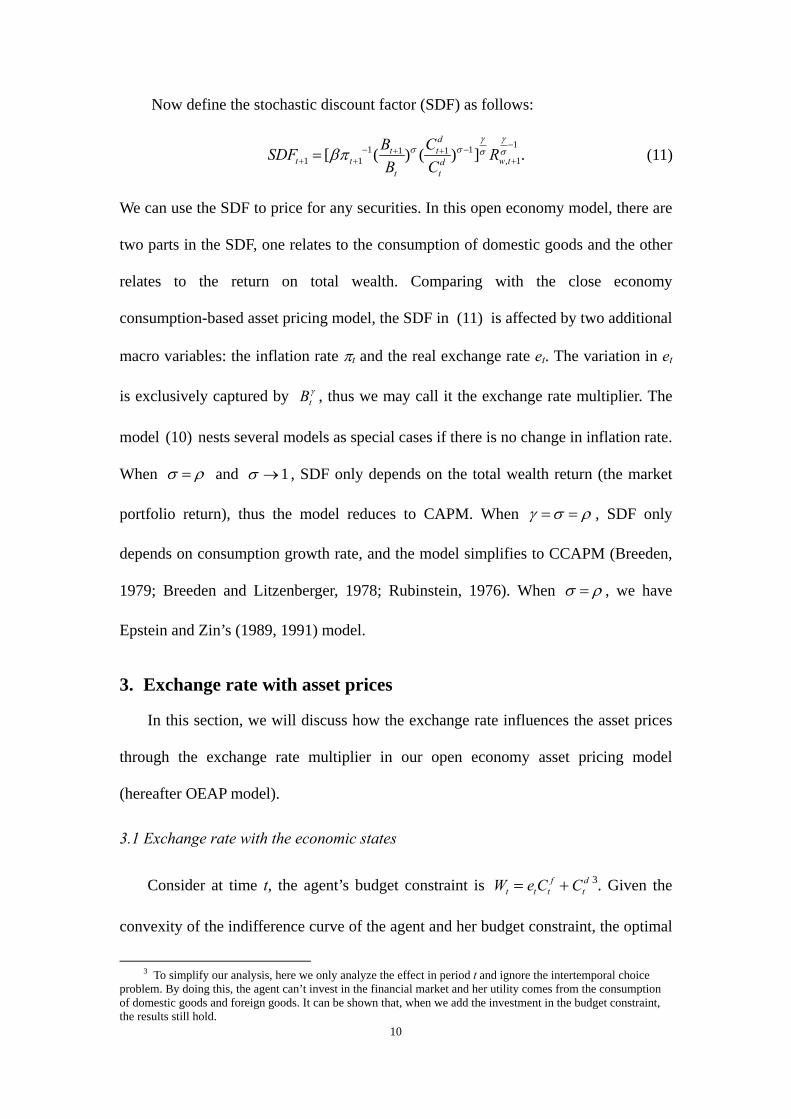
model (10) nests several models as special cases if there is no change in inflation rate.

When and 1 , SDF only depends on the total wealth return (the market

portfolio return), thus the model reduces to CAPM. When , SDF only

depends on consumption growth rate, and the model simplifies to CCAPM (Breeden,

1979; Breeden and Litzenberger, 1978; Rubinstein, 1976). When , we have

Epstein and Zin’s (1989, 1991) model.

3. Exchange rate with asset prices

In this section, we will discuss how the exchange rate influences the asset prices

through the exchange rate multiplier in our open economy asset pricing model

(hereafter OEAP model).

3.1 Exchange rate with the economic states

Consider at time t, the agent’s budget constraint is f dt t t tW e C C 3. Given the

convexity of the indifference curve of the agent and her budget constraint, the optimal

                                                              3 To simplify our analysis, here we only analyze the effect in period t and ignore the intertemporal choice

problem. By doing this, the agent can’t invest in the financial market and her utility comes from the consumption of domestic goods and foreign goods. It can be shown that, when we add the investment in the budget constraint, the results still hold.

11  

consumption bundle is shown as x1 in Figure 1. Now, considering the effect when the

real exchange rate et decreases, the value of foreign goods will be lower than before.

There are two effects with the exchange rate changes: income effect and substitution

effect. The income effect will cause the budget line to move outwards, and make the

agent to achieve a higher level of consumption bundle x2, which is preferable to the

old bundle x1, and the agent is no worse than before. On the contrary, when the real

exchange rate increases, the budget line will move inside, which makes the

consumption bundle x1 cannot be chosen, and the utility her can achieve is lower than

before. That is, the real exchange rate et has a negative relation with the utility level.

Further, it is known that the consumption has the procyclical property, it is higher in

good state than in bad state, thus, the real exchange rate et has a countercyclical

property. More precisely, when the economy is in good state, the exchange rate will

appreciate, when the economy is in bad state, the exchange rate will depreciate. This

finding is the same as what is known in the macroeconomics literature.

In Figure 2, we illustrate the variation of the real effective exchange rate (REER)

index of Chinese RMB from Jan 1997 to Dec 2010. The shaded regions are economic

recessions, which are defined in terms of four consecutive quarters of decline in real

GDP growth rate or a quarter decline in real GDP. The GDP and CPI data are both

collected from the National Bureau of Statistics of China to calculate the real GDP.

The REER index is provided by the Bank of International Settlement (BIS). A high

value of this index means the real exchange rate appreciation and a low value

indicates the depreciation. So here it is equivalent to the reciprocal of the real

exchange rate et. This figure reveals a relationship between the real exchange rate and

business cycles. The index decreases slightly twice in recessions during 1997 and

1998. During and after the recession in 2002-2003, the real exchange rate index

12  

decreases sharply, then the index experiences a steadily increase till 2009. Finally, the

index trends downwards in the 2009-2010 recession period. Overall, we can conclude

that the real exchange rate depreciates coincides with recessions and it appreciates

sharply during expansions. This is consistent with the results found in Guillaumont

and Hua (2001) and Wang and Yao (2003). And it also empirically supports our

previous analysis that exchange rate et is countercyclical.

3.2 Exchange rate multiplier, economic states and consumption

To have a better understanding of the exchange rate multiplier tB with

economic states and consumption, we first assume the risk aversion parameter , the

parameter for elasticity of intertemporal substitution , and the parameter for

elasticity of substitution between domestic and foreign goods satisfy the relation:

0 , 0 . These assumptions require that the relative risk aversion (1-) is

greater than 1, which is consistent with the empirical findings in the large equity

premium literature (see Mehra and Prescott, 2003). The relation 0 implies

that the EIS < ES < 1. When these two conditions have been satisfied, we show in the

Appendix B that the exchange rate multiplier tB is an increasing function of et.

Because of the countercyclical property of et, tB is countercyclical as well. Now we

can combine the relation among the exchange rate multiplier, economic states and

consumption together, we have the following Lemma 1:

Lemma 1: When the conditions 0 , 0 hold, we have:

When the economy is in boom, the total consumption increases, the real exchange rate

appreciates and the exchange rate multiplier decreases;

When the economy is in recession, the total consumption deceases, the real exchange

rate depreciates and the exchange rate multiplier increases.

13  

Lemma 1 is the foundation for our analysis of the exchange rate on asset prices.

3.3 Exchange rate variation and asset’s risk

In the consumption-based asset pricing models, the risk-averse agent faces the

volatility of consumption due to economic fluctuation. She wants to trade in assets to

substitute and smooth the consumption over time and across states. In states of nature

when future consumption turns out to be high (due to high asset returns or high labor

income), the marginal utility is low and the asset’s payoffs in these states are not

highly valued. Conversely, when future consumption is low, the marginal utility is

high and the asset’s payoffs in these states are much desired. That is to say, the risks

of assets are determined by the negative relationship between the asset returns and the

marginal utility. Agent would claim higher excess return to compensate her risk to

hold these assets. In conclusion, the above relation could be expressed in the language

of asset pricing model as:

1 1 1 1 1 1 1 1( ) cov( , ) cov( ( ) ( ), ),jt ft ft t jt ft t jtE R R R SDF R R f MU C R  

where Rft+1 is the risk-free rate, 1( )tMU C is the marginal utility of consumption,

and ( )f is a function of variables which relates to the setting of utility function.

In our open economy setting, the variation in the real exchange rate will have

impact on asset prices through the SDF, more precisely, through tB

  in equation (11).

In good state, the appreciation of real exchange rate will decrease tB and then

decrease the marginal utility; while in bad state, the depreciation of real exchange rate

will increase tB and eventually increase the marginal utility. In both states, the

exchange rate will strengthen the negative relationship between asset return and

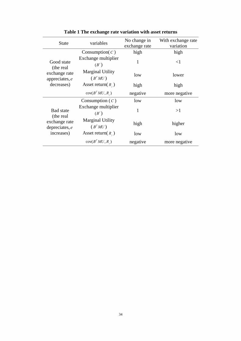
marginal utility, thus increase the risks of investors. Table 1 illustrates the relationship

between the real exchange rate variation and the asset’s risks in different states.

14  

4. Data

We use three sets of assets in estimating the OEAP model for Chinese stock

market. The first set consists of 25 portfolios of all A-shares traded in Shanghai and

Shenzhen Stock Exchange. The 25 portfolios are 5x5 size and book-to-market equity

ratio according to Fama and French (1992, 1993) sorting criteria. The second group of

assets includes 14 portfolios following CITIC industrial classification standard4. We

also consider 5 size portfolios when study the time-varying property of asset returns

with exchange rate. The all A-shares return is used as the wealth portfolio return. The

risk-free interest rate is the 3-month saving rate. All of the above data are provided by

RESSET Financial Research Database.

The total retail sales of consumer goods, the nominal RMB exchange rate against

US dollar, the total imports and the CPI are collected from the China Economics

Information Network. We screen our data by first eliminating the products used for

reproduction from the total imports to get the final import goods for consumption. Our

screen rule is based on standard international trade classification (SITC) to make the

category of exports and retail sales to be much more consistent.5 Then the domestic

consumption goods can be drawn by taking the difference between the total retail

sales and the final consumed import goods. The consumption data are adjusted to

per-capita level by monthly population and CPI. The population data are from the

annually Statistical Yearbook provided by National Bureau of Statistics of China. We

assume the population increases in a geometric ratio, then the number of monthly

population can be easily calculated. Inflation is computed as monthly changes of the

seasonally adjusted CPI.

                                                              4 The CITIC industrial classification standard is provided by CITIC Securities Company. The industry

classification has been widely used in Chinese academia. 5 Specifically, we omit crude materials tagged in code 2, Mineral fuels tagged in code 3, all items tagged in

code 5 except for medicinal and pharmaceutical products, manufactured goods classified chiefly by material tagged in code 6 and all items tagged in code 7 except for road vehicles.

15  

We also need to consider the instrumental variables when studying the

time-varying property of asset returns and exchange rate. There are several candidates

we can use following the literature. Besides the frequently used: one lag of the

domestic consumption growth rate, price-earnings ratio (P/E), size spread (the

difference between the average return of the 5 smallest size group and that of the 5

largest size group), and yield spread (the 5-year saving rate over 3-month saving rate),

we will consider the one lag of the exchange rate change in our model. We hope these

5 variables can capture the time-varying property of asset returns.

The data period is from January 1997 to December 2010, and monthly frequency

is used.

5. Estimation and testing of the open economy asset pricing model

5.1 The GMM estimation results

To estimate the preference parameters in the Euler equation (10) and test the

model, we follow Hansen and Singleton’s (1982) GMM methodology. Since equation

(10) holds for all the securities, it holds for the risk-free asset. Thus, we have the

following moment conditions for risky assets and risk-free asset:

1 1[ ( 1)] 0,t ftE SDF R (12)

1 1 1[ ( )] 0, 1, 2,..., .t jt ftE SDF R R j N (13)

Equation (12) represents 1 moments restrictions implied by the Euler equation for the

risk-free asset. Equation (13) represents N moment restrictions implied by the Euler

equations for N portfolio returns. There are five parameters ( , , , , and ) to be

estimated from a total of N+1 moment restrictions. The ( 1) 5N overidentifying

restrictions can be tested through the J-test.

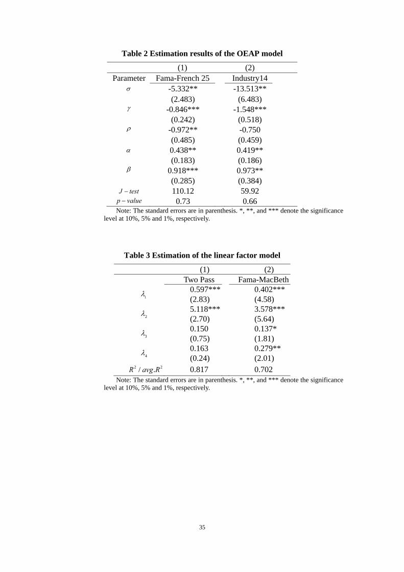
Table 2 presents our GMM estimation results using 25 Fama-French portfolio and

16  

14 Industry portfolios. In the results for 25 Fama-French portfolios, σ = -5.332, which

implies that the elasticity of intertemporal substitution is 0.158. ρ = -0.972 indicates

the elasticity of substitution has the value of 1/ (1 ) 0.507ES . 0 1ES

represents a lower substitution effect between the domestic goods and foreign goods.

When the real exchange rate et decreases, from equation (8), we know that the

proportion of domestic goods value will increase in the total expenditure. The

estimate for is -0.846, thus the risk aversion coefficient 1 1.846 , which is in

the reasonable range suggested by Mehra and Prescott (1985). In short, the estimation

results show that 0 , 0 , which is consistent with the conditions we

discussed in Lemma 1. 

Parameter measures the subjective preference of foreign goods over domestic

goods. The estimation result for is 0.438, this low value of means that investors

prefer domestic goods more. Considering the effect of exchange rate on asset prices, a

low value of also indicates that the volatility of domestic goods should play a more

important role to determine asset prices. The time preference parameter 0.918 1 ,

which can avoid Hall’s (1988) risk-free rate puzzle. In the overidentification test, the

p-value for J-statistic is 0.73, which does not reject the model.

When using the 14 industry portfolios to re-estimate the model, we find the

results are quite similar as those for the 25 Fama-French portfolios. The risk aversion

parameter (), the EIS parameter () and ES parameter () satisfy the relation 0 ,

0   as well.  The only problem is that, in this case, is not statistically

significant. The p-value of 0.66 for overidentification test states that we can’t reject

the model.

Above all, results in Table 2 show that the OEAP model can price the 25

17  

Fama-French portfolios and 14 industry portfolios in Chinese stock market, and the

parameters satisfy the relation that 0 , 0 .

5.2 Exchange rate risk and asset prices

We have used the GMM method to estimate the parameters and test the open

economy model. In this subsection, we want to test the cross-sectional implications of

the OEAP by approximating it as a linear factor model and discuss the exchange rate

risk with the asset returns. The main advantage of the linear factor model is that we

can explicitly find out the contribution of exchange rate risk in explaining asset

returns. And it also makes the results readily comparable with the large cross-sectional

asset pricing literature, which focuses on linear factor models.

5.2.1 Linear factor model

Appendix C shows that the unconditional Euler equation (10) can be

approximated as a linear factor model

1 2

3 4

[ ] cov( log( ), ) cov( log( ), )

cov( log( ), ) cov(log( ), ),

djt ft t jt ft t jt ft

t jt ft wt jt ft

E R R b e R R b C R R

b P R R b R R R

(14)

in which 1b , 2 (1 )b

, 3b

, and 4 1b

. This equation says that

the premium on asset j is the price of risk bk times its quantity of risk

cov( , )kt jt ftf R R , where kf denotes the k-th factor.

Further, denoting ( )k k ktb var f , and the vector of , 1,... ,k k K equation

(14) can be expressed as the following beta version:

[ ] 'jt ft jE R R , (15)

where 1' ( ,..., )j j jK captures the risk exposure of the asset j to the K factors,

4K in our model. Especially, for the k-th factor, we have

18  

cov( , ) / var( )jk kt jt ft ktf R R f . In this beta relation, k is usually called the risk

premium or risk price associated with factor kf .

Equation (14) and equation (15) tell us that an asset with high exchange rate beta,

cov( log( ), ) / var( log( ))t jt ft te R R e , must have high expected returns when

1 0b . Since 1b , the risk premium of exchange rate 1 var( log( ))te

must be positive as long as 0 , which has already been justified in Table 2.

Following our definition of the exchange rate beta, it tells us that an asset will have a

high exchange rate beta if the asset return is high during the appreciation of the real

exchange rate (i.e., log( ) 0te ), and the asset return is low during the depreciation

of the real exchange rate. This result is the same as what we addressed in Table 1.

The domestic consumption growth beta, inflation rate beta and market portfolio

beta with the asset premium have the similar explanation. In equilibrium, differences

in expected returns across assets must reflect differences in the quantity of risk across

assets, measured by of the exchange rate and other factors.

5.2.2 Estimation of the linear factor model

We use the two-pass regression and Fama-MacBeth (1973) method to estimate

the linear factor model (15). The portfolio we used is the 25 Fama-French portfolios.

The first column in Table 3 reports the estimate results of the two-pass regression. The

exchange rate and consumption growth rate both have significantly positive risk price

(1=0.597 and 2=5.118), which means that investors require risk compensation for

their bearing of the exchange rate risks and consumption risks. Furthermore, investors

require higher return for those assets that have positive exchange rate beta, because

holding those assets make their consumption more volatile. Specifically, the returns

on those assets will increase when the real exchange rate appreciates (in boom) and

19  

decrease when the real exchange rate depreciates (in recession).

The second column in Table 3 shows the estimation results using Fama-MacBeth

(1973) methodology. The estimation results are similar as that of the two-pass

regression, except that the risk premia of inflation rate and market portfolio return are

statistically significant at least at 10% level. The difference may rely on the fact that

Fama-MacBeth methodology considers the time-varying prices of risk here. Above

all, the two regression results show that the exchange risk does contribute to the

asset’s risk premium. And the high R2 for two-pass regression and the average R2 for

Fama-MacBeth method suggest that our four factor model can largely explain the

cross-sectional variation of those 25 portfolio returns.

Panel A of Figure 3 provides a visual summary of the empirical success of the

OEAP model. On the vertical axis is the realized average return. On the horizontal

axis is the return predicted by the model, based on the two-pass regression results.

The straight line is the 45 degree line that all the portfolios should locate on. The dots

represent the 25 Fama-French portfolios, and the corresponding vertical distance to

the 45 degree line represents the pricing error. The diagram reveals that the pricing

errors are very small and the OEAP model fits the data very well.

Panel B of Figure 3 shows the relationship between exchange risks with the asset

returns. The vertical axis is the average portfolio return, and the horizontal axis is the

exchange risk. The dot represents the exchange risk beta for each portfolio, which

comes from the first-step in the two-pass regression. The slope of the fitted line

measures the risk price of the exchange rate 1 . This upward slope shows that the

asset expected return has a positive relation with the exchange risk premium. Another

important feature we may notice in Panel B is that all the small size portfolios locate

at the right-top area of the graph, which indicates that they have higher exchange risks

20  

comparing with other portfolios, and the high risk premium in small size group can be

partly explained by the exchange rate risks.

5.3 Time variation in expected asset returns

A large literature in asset pricing finds that the stock returns are time-varying.

The asset returns are high during economic recession and low during economic

expansion (Campbell and Clarida, 1987; Campbell and Shiller, 1987; etc). Many

studies try to understand this countercyclical property. In a factor pricing model, the

time variation in the expected return must be explained by the time variation in the

quantity of risk. On the other hand, as we have stated in the introduction, many works

have documented that the exchange rate risk is changing over time, and studied the

conditional factor model. In this subsection, we will discuss the exchange rate risk

with the time varying expected returns. Firstly, based on Campbell and Clarida (1987),

and Campbell and Shiller’s (1987) finding, we want to investigate whether Chinese

stock returns have the countercyclical property. Secondly, we want to investigate the

relation of exchange rate risk with the business cycle and to find out whether the

exchange risk can explain the countercyclical expected returns.

Vershink (1964) shows that if the joint distribution of asset excess returns and the

instrumental variables are spherically invariant, the excess returns can be written as

the linear function of the instrumental variables

1' , 1,..., ,jt t jtr Z u j N (16)

where jtu is the forecasting error, jt jt ftr R R is the excess return for asset j, 1tZ

is the 1I instrumental variable vector and is the 1I coefficient matrix.

When a proper set of instrumental variable has been chosen to capture the economy

states, we can use equation (16) to study the cyclical property of asset returns.

21  

Following Cochrane (1996), Lettau and Ludvigson (2001) and many others, we

can scale the factors in the conditional version of the linear factor model (15), and

beta coefficients can be expressed as a linear function of the instrumental variables,

we have

1 ,jt t jtZ v (17)

where jtv is 1K estimation error vector and is the I K coefficient matrix.

Panel A in Table 4 reports the estimation results of portfolio returns on the

instrumental variables according to equation (16). Here, we focus on 5 size portfolios.

We select five instruments that may proxy for economic status and predict future

expected returns: the first is lagged real exchange rate change, which is based on our

illustration in section 3.1. The other variables we used are one lag of the consumption

growth rate, price-earnings ratio, size spread, yield spread and a constant. Each

column in Panel A represents the estimate coefficient of the instrumental variables on

the 5 size portfolio returns. In the first 4 size portfolios, the coefficients of lagged

exchange rate are significantly positive, and the coefficients of lagged consumption

growth rate are significantly negative. These results show that the real exchange rate

change and the consumption growth rate both have power in forecasting stock returns.

It is noted that the real exchange rate depreciation and the low consumption growth

capture the downturn in economy, accompanying with a large consumption decrease.

Thus investors require a higher risk premium for holding assets. In short, the estimate

result shows that stock returns have countercyclical property in Chinese stock market.

All the estimate coefficients with price-earnings ratio are significantly positive.

This indicates that P/E ratio has power in predicting asset returns, and the finding is

consistent with the asset return predictability literature (see e.g. Basu, 1977; Campbell

and Shiller, 1988; Fama and French, 1988). The coefficients on the yield spread are

22  

negative, implies that this countercyclical variable would induce a higher expected

return in recession. Such finding is consistent with the result found in Campello, Chen

and Zhang (2008). However, all the coefficients with size spread are not statistically

significant.

Panel B of Table 4 reports the relation of the exchange risk beta with the

instrumental variables according to equation (17). The exchange rate beta we used is

from the first-pass in the two-pass regression on the 5 size portfolios. The results state

that all the coefficients of the real exchange rate change are positive, and all the

coefficients with consumption growth rate are negative, especially in these smaller

size portfolios. These finding demonstrates that in bad state, i.e. when consumption is

low or the real exchange rate depreciation, stocks would have a higher exchange rate

risk. Combining with the results in Panel A, we may draw the conclusion that both

exchange risk and asset premium are countercyclical, and the countercyclical property

in asset premium can be partly explained by the countercyclical property in exchange

risk. The time-variation in asset return can be partly explained by the time-variation in

exchange risk. 

5.4 Further analysis

In July 2005, the Chinese authority has the reform of RMB exchange rate system.

While the currency remains effectively pegged to a basket of hard currencies, it is

allowed to fluctuate against the US dollar by less than 0.3% per day in either direction

since then. The RMB exchange rate would show different characteristics before and

after the reform6 (see, Shah, Zeileis and Patnaik, 2005; Ogawa and Sakane, 2006). In

this subsection, we divide our sample into two sub-periods according to the reform

and compare the relationship of the stock returns with the exchange risks before and

                                                              6 Our data shows that the volatility of RMB exchange rate increases 13% after the reform.

23  

after the reform.

Panel A in Table 5 represents the return changes before and after the reform for

the 25 Fama-French portfolios. Firstly, the differences for all the portfolios are greater

than 0, which means that assets returns are higher after the reform. Secondly, reading

down the columns of the panel, the differences in returns decrease in size for a given

book-to-market equity quintile, indicating that small stocks have more premium than

big stocks after the reform. However, reading across the rows of the panel, the

differences in returns is not related to book-to-market equity in a consistent way for a

given size quintile.

Since the increasing exchange rate volatility after the reform, we should examine

whether the observed phenomenon showed in Panel A are the results of the increased

exchange risks after the reform. Thus, in Panel B of Table 5, we calculate the

difference of exchange risk before and after the reform for each portfolio. The

estimates of exchange risks e are based on the results in the first step of the

two-pass regression. The results show that nearly all the portfolios’ exchange risks

increase after the reform, except for the “big-high” portfolio. And the differences are

much larger in the small size groups than those in the big size groups, which imply

that the exchange risks increase more for the small size groups.

To summarize, we find that the increased risk premium after the reform can be

explained by the increased exchange risk. The increased exchange risk has more

impact on the small size group comparing with the large size group, which reconfirms

that the exchange rate risk indeed contributes to the cross-sectional size premium. 

6. Conclusion

In this paper, we develop an equilibrium consumption-based asset pricing model

in an open economy framework. The real exchange rate affects the asset returns

24  

through the marginal utility of consumption. It will increase the risks the investor

facing comparing with the close economy. To our knowledge there is no previous

study that investigates the exchange risk considering investor’s consumption and

portfolio decision. Our empirical estimations demonstrate that this model can

successfully price the 25 Fama-French portfolios and industry portfolios in Chinese

stock market. The exchange risk is a risk factor in the unconditional linear factor

model and can contribute to explain asset returns. Even though we do not directly test

the conditional linear factor model, we find evidence that both the exchange risk and

asset return are time-varying and have countercyclical property in Chinese stock

market. The countercyclical exchange risk can help to explain the countercyclical

asset returns.

Our study has important implication for investment and risk management for

investors in emerging markets. The exchange risk is non-diversifiable and investors

require compensation for taking this type of risk, especially in those economies that

face foreign currency restrictions. Also, we need to consider the time-varying property

in exchange risk.

 

25  

Appendix A: Derivation of the Stochastic Discount Factor

A.1 The optimal choice of dtC

The optimization problem for the agent with the budget constraints is as follows:

 

1

1

/1 1

1 1

}

. .

{(1 )[(1 )( ) ( ) ] [ ( ( ) )]

( )

1 1,2,...,& ,

d ft t t t t

f dt t t t t t t t

jN

jt

J Max C C E J W

W W e C C R

t T

s t

  (A.1) 

where J is the value function of this Bellman equation. We conjecture J has the form

that ( )t t tJ W W , which represents that the value function is a proportion of the total

wealth. Taking the first order condition with respect to dtC in equation (4), i.e.

0dt

U

C

, we have:

1

1 111 [ 1 ) ( ][ 1 ) ) ) ] () ) ][ .d d f f d

t t t t t t t t t wtC C C W e C C E R

（ （ （ （

And for the FOC with respect to ftC , 0

ft

U

C

, we have:

1

1 111 [ ( ) ][(1 )( ) ( ) ] ( ) ] .[d d f f d

t t t t t t t t t wt tC C C W e C C E R e

Take the ratio of these two equations, we have: 

1

1(1 )[ ] , ( ,1).

ft tdt

C e

C

(A.2)

The total consumption value at time t can be expressed as f dt t te C C . Using (A.2)

to substitute the expression of ftC , the total consumption can be written as

1 1

1 1 11 ) 1[ ] [1 ) ].f d d d dt

t t t t t t t t

ee C C e C C C e

（

（ (A.3)

Let 1

1 111 )t tA e

（ , equation (A.3) has a expression of

26  

1

.dt

f dt t t t

C

A e C C

(A.4)

Further, if we substitute (A.2) and (A.4) into the utility function (4), the utility

function of domestic goods and foreign goods can be expressed as a function of tA :

1 1

( , ) [(1 )( ) ( ) ] ([ 1 ) ] .f d d f dt t t t t tu C C C C C A (A.5)

Now, Let’s back to the optimization problem (A.1) and consider the conjecture of

t , we have:

1 1 1 1 1( )( ) ( ) ( ) ,dt t t t t t t t t tJ W W AC R (A.6)

where t tR is the optimal portfolio return and represents the total wealth return.

Denote wt t tR R , substitute (A.5) and (A.6) into the optimization problem (A.1),

and take the first order condition w.r.t dtC , we have:

1 1 *(1 )[(1 ) ] (( ) () ) ,d dt t t t t tA C W AC A

(A.7)

where 1

*1 1( [ ])t t t wtE R . Further assume that t

dt tC W , which says that the

optimal consumption of domestic goods is a proportion of total wealth. From (A.7),

*( ) takes the form of

1

*1

(1 ) (1 )( .

( ))

1t t

t t t

A

A A

(A.8)

Now, substituting (A.8) back to the Bellman equation (A.1), we have:

1

1

(1 ) (1 ).

(1( ) (1 )( ) [(1 ) ] (1 )

)t t

t t tt

tt t

dt t t

A

AA A

AW WC

And rearrange it,

1 1 1

1[(1 )(1 ) ] .t t tA

(A.9)

27  

Let 11

[(1 )(1 ) ]t tB A

, and we have:

1 11 1

)dt

t t t tt

CB B

W

（ .

Substitute t into the expression of * , then take it back to (A.7), after the

rearrangement, we have:

1 11 11([ ) ) ] 1

dt t

t t wtdt t

B CE R

B C

（ , (A.10)

This equation determines the optimal choice of dtC .

A.2 The optimal choice of the portfolio t

It can be shown that when determining the optimal portfolio choice t , the

Bellman equation (A.1) is equivalent to

1

1 1

1

max[ ( ) ]

. . 1,

t t t

Nj jt

V E J W

s t

(A.11)

where 11 1 1 1 1 1(( ) )d

t t t t t t t t t t tJ W W W AC R

.

Now let’s consider the first asset, 1j . Denote 1 21 Nt j jt , substitute it

back to the budget constraint and take the first order condition w.r.t to jt in (A.11),

we have:

1

11 1 1

1 1 1 1 1

1 ([ ( ) 0, 1] .)t t t t t t t jt t

jt

dVV E R R R j

d

(A.12)

Take the expression of t in (A.9) into (A.12)

1

1(1 ) 1

1 11[( ) ( ) ( )] 0, 1.

t

dt t

t wt jt tdt t

B CE R R R j

B C

(A.13)

Together with what we have in (A.10), for any assets 1j , they satisfy the condition

that

28  

1

(1 ) 11 1

1 1[ ( ) ,) ] 1( 1 .d

t tt t wt td

t t

B CE R R j

B C

(A.14)

Similarly, when 2, ...,j N , we have the similar results. Thus, for all the assets, we

have:

1

(1 ) 11 1

1 1 1 1,2,...,[ ( ) ( ) ] .d

t tt t wt jtd

t t

B CE R R j N

B C

， (A.15)

Define the stochastic discount factor 11 11 1

1 1 1[ ( )( ) .]d

t tt t wtd

t t

B CSDF R

B C

(A.15)

states that we can use the SDF to price for any securities.   

Appendix B: The proof that the exchange multiplier 1( )tB is an

increasing function of 1te

In Section 3.2, we want to show that when 0 , 0 , 1( )tB is an

increasing function of 1te .

Proof: We have 1

[(1 )(1 ) ]t tB A

and

1

1 111 )t tA e

（ , it can be

shown that 

1 2( )[(1 )( ) ] ( 1) 0t

t tt

d BA A

dA

,

and 1 1

1 11( ) ( ) 0

1t

tt

dAe

de

.

Thus, we have( )

0t

t

d B

de

, and 1( )tB is an increasing function of 1te . 

Appendix C: The linear factor model of the OEAP model

Consider the expression of SDF in (11):

11 1

1 1

[ ( ) ( ) ]d

t tt t wtd

t t

B CSDF R

B C

. (C.1)

29  

Let 1

( ) (1 )(1 ) ( )t tB V e

and 1

1(1 )( ) [1 ( ) ]t

t

eV e

, SDF

can be expressed as

( ) ( 1) 1

1 1

( )[ ] ( ) .

( )

dt t

t wt tdt t

V e CSDF R

V e C

(C.2)

Take the logarithmic at both sides and consider when 0 , we have:

0

lim log( ) log log( ) ( 1) log( )

( 1) log( ) log( )

dt t t

wt t

SDF e C

R P

, (C.3)

where 1

log( ) log( )tt

t

ee

e

,1

log( ) log( )d

d tt d

t

CC

C

and 1

log( ) log( ) log( )tt t

t

PP

P

.

Following the treatment in Yogo (2006), the SDF can be written as

11

1 log( ) [log( )][ ]

tt t t

t t

SDFSDF E SDF

E SDF

. (C.4)

Substituting (C.3) into (C.4), the SDF of OEAP model takes a linear factor version:

1 2 3 41

log( ) log( ) log( ) log( )[ ]

dtt t t wt

t t

SDFk b e b C b P b R

E SDF

, (C.5)

in which,

1 [ log( )] ( 1) [ log( )] [ log( )] ( 1) [log( )]dt t t t t t t wtk E e E C E P E R

and 1b ， 2 (1 )b

， 3b

， 4 1b

.

Furthermore, we can use the vectors to simplify the expression in (C.5):

1

,[ ]

tt

t t

SDFk b f

E SDF

(C.6)

where 1 4( , ..., )b b b and the factor vector

( log( ), log( ), log( ), log( ))dt t t t wtf e C P R .

Moreover, for any assets we have [ ( )] 0t jt ftE SDF R R , and

30  

1

[ ] [ ] cov( , )

[ ] cov( , )[ ]

cov( , ) cov( , ).

t jt ft t jt ft

tjt ft jt ft

t t

t jt ft t jt ft

E SDF E R R SDF R R

SDFE R R R R

E SDF

k b f R R b f R R

(C.7)

The linear factor model of OEAP takes the form of

1 2

3 4

( ) cov( log( ), ) cov( log( ), )

cov( log( ), ) cov(log( ), )

djt ft t jt ft t jt ft

t jt ft wt jt ft

E R R b e R R b C R R

b P R R b R R R

. (C.8)

31  

References:

Abuaf, N., Jorion, P., 1990. Purchasing power parity in the long run. Journal of Finance 45(1), 157-174.

Basu, S., 1977. Investment performance of the common stocks in relation to their price-earning ratios: a test of efficient market hypothesis. Journal of Finance 32(3), 663-682.

Breeden, D.T., 1979. An intertemporal asset pricing model with stochastic consumption and investment opportunities. Journal of Financial Economics 7, 265-296.

Breeden, D.T., Litzenberger, R.H., 1978. Prices of state-contingent claims implicit in option prices. Journal of Business 51, 621-651.

Campbell, J.Y., Clarida, R.H., 1987. The term structure of euromarket interest rates: an empirical investigation. Journal of Monetary Economics 19(1), 25-44.

Campbell, J.Y., Shiller, R.J., 1987. Cointegration and tests of present value models. Journal of Political Economy 95(5), 1062-1088.

Campbell, J.Y., Shiller, R.J., 1988. The dividend-price ratio and expectations of future dividends and discount factors. Review of Financial Studies 1, 195–227.

Campello M., Chen, L., Zhang, L., 2008. Expected returns, yield spreads, and asset pricing tests. Review of Financial Studies 21(3), 1297-1338.

Carrieri, F., 2001. The effects of liberalization on market and currency risk in the EU. European Financial Management 7(2), 259-290.

Carrieri, F., Majerbi, B., 2006. The pricing of exchange risk in emerging stock markets. Journal of International Business Studies 37, 372–391.

Chaieb, I., Mazzotta, S., 2013. Unconditional and conditional exchange rate exposure. Journal of International Money and Finance 32, 781-808.

Claessens, S., Dusgupta, S., Glen, J., 1998. The cross-section of stock returns: evidence from emerging markets. Emerging Markets Quarterly 2, 4–13.

Choi, J.J., 1986. A model of firm valuation with exchange exposure. Journal of International Business Studies 17(2), 153- 159.

Choi, J.J., Hiraki, T., Takezawa, N., 1998. Is foreign exchange risk priced in the Japanese stock market? Journal of Financial and Quantitative Analysis 33(3), 361-382.

Cochrane, J.H., 1996. A cross-sectional test of an investment-based asset pricing model. Journal of Political Economy 104, 572-621.

Cohen, R.B., Polk, C., Vuolteenaho, T., 2003. The value spread. Journal of Finance 58, 609–641.

De Santis, G., Gerard, B., 1998. How big is the premium for currency risk. Journal of Financial Economics 49(3), 375-412.

Doukas, J., Hall, P., Lang, L., 1999. The pricing of currency risk in Japan. Journal of Banking and Finance 23(1), 1-20.

Dumas, B., 1978. The theory of the trading firm revisited. Journal of Finance 33(3), 1019-1029.

Dumas, B., Solnik, B., 1995. The world price of foreign exchange risk. Journal of Finance 50(2), 445-479.

Epstein, L.G., Zin, S.E., 1989. Substitution, risk aversion and the temporal behavior of consumption and asset returns: a theoretical framework. Econometrica 57(4), 937-969.

32  

Epstein, L.G., Zin, S.E., 1991. Substitution, risk aversion and the temporal behavior of consumption and asset returns: an empirical analysis. Journal of Political Economy 99, 263-286.

Fama, E.F., French, K.R., 1988. Dividend yields and expected stock returns. Journal of Financial Economics 22, 3–27.

Fama, E.F., French, K.R., 1992. The cross-section of expected stock returns. Journal of Finance 47, 427-465.

Fama, E.F., French, K.R., 1993. Common risk factors in the returns on stocks and bonds. Journal of Financial Economics 33, 3-56.

Fama, E.F., MacBeth, J.D., 1973. Risk, return, and equilibrium: empirical tests. Journal of Political Economy 81(3), 607-636.

Grossman, S.J., Melino, A., Shiller, R.J., 1987. Estimating the continuous-time consumption-based asset-pricing model. Journal of Business and Economic Statistics 5(3), 315-327.

Guillaumont J.S., Hua, P., 2001. How does real exchange rate influence income inequality between urban and rural areas in China? Journal of Development Economics 64 (2), 529-545.

Hall, R.E., 1988. Intertemporal substitution in consumption. Journal of Political Economy 96(2), 339-357.

Hamao, Y., 1988. An empirical examination of arbitrage pricing theory: using Japanese data. Japan and the World Economy 1(1), 45-61.

Hansen, L.P., Singleton, K.J., 1982. Large sample properties of generalized method of moments Estimators. Econometrica 50(4), 1029-1054.

Hansen L.P., Singleton, K.J., 1983. Stochastic consumption, risk aversion, and the temporal behavior of asset returns. Journal of Political Economy 91(2), 249-265.

Jacobsen, B.J., Liu, X., 2008. China’s segmented stock market: an application of the conditional international capital asset pricing model. Emerging Markets Review 9(3), 153-173.

Jorion, P., 1991. The pricing of exchange rate risk in the stock market. Journal of Financial and Quantitative Analysis 26, 363–376.

Kodongo, O., Ojah, K., 2011. Foreign exchange risk pricing and equity market segmentation in Africa. Journal of Banking and Finance 35, 2295-2310.

Kolari, J.W., Moorman, T.C., Sorescu, S.M., 2008. Foreign exchange risk and the cross section of stock returns. Journal of International Money and Finance 27, 1074–1097.

Lettau, M., Ludvigson, S., 2001. Resurrecting the (C)CAPM: a cross-sectional test when risk premia are time-varying. Journal of Political Economy 109, 1238–1287.

Li, K., 1999. Testing symmetry and proportionality in PPP: a panel-data approach. Journal of Business and Economic Statistics 17(4), 409-418.

Lucas, R.E., 1978. Asset pricing in an exchange economy. Econometrica 46, 1426-1445.

Mehra, R., Prescott, E.C., 1985. The equity premium: a puzzle. Journal of Monetary Economics 15(2), 145-161.

Mehra, R., Prescott, E.C., 2003. The equity premium in retrospect. In Constantinides, G.M., Harris, M., Stulz, R. (Eds.), Handbook of Economics and Finance, North-Holland, Amsterdam, 887-936.

Ogawa E, Sakane M., 2006. Chinese yuan after Chinese exchange rate system reform. China & World Economy 14(6), 39-57.

33  

Phylaktis, K., Ravazzolo, F., 2004. Currency risk in emerging equity markets. Emerging Markets Review 5, 317–339.

Roll, R., 1979. Violations of purchasing power parity and their implications for efficient international commodity markets. In Sarnat, M., Szego, G.P. (Eds.), International Finance and Trade, Ballinger, Cambridge, MA, 133-176.

Rubinstein, M., 1976. The valuation of uncertain income streams and the pricing of options. Bell Journal of Economics 7, 407-425.

Salehizadeh, M., Taylor, R., 1999. A test of purchasing power parity for emerging economies. Journal of International Financial Markets, Institutions and Money 9(2), 183-193.

Shapiro, A.C., 1974. Exchange rate changes, inflation, and the value of the multinational corporation. Journal of Finance 30(2), 485-502.

Shah, A., Zeileis, A., Patnaik I., 2005. What is the new Chinese currency regime? WU Vienna University of Economics and Business, Working paper.

Solnik, B., 1997. The world price of foreign exchange risk: some synthetic comments. European Financial Management 3(1), 9- 22.

Tai, C.S., 1999. Time-varying risk premia in foreign exchange and equity markets: evidence from Asia-Pacific countries. Journal of Multinational Financial Management 9, 291-316.

Vassalou, M., 2000. Exchange rate and foreign inflation risk premiums in global equity returns. Journal of International Money and Finance 19(3), 433-470.

Vershink, A.M., 1964. Some characteristics properties of Gaussian stochastic processes. Theory of Probability and Its Applications 9, 353-356.

Wang, Y., Yao, Y., 2003. Source of China’s economic growth, 1952-99: incorporating human capital accumulation. China Economic Review 14(1), 32-52.

Yogo, M., 2006. A consumption based explanation of expected stock returns. Journal of Finance 61(2), 539-580.

34  

Table 1 The exchange rate variation with asset returns

State variables No change in exchange rate

With exchange rate variation

Good state (the real

exchange rate appreciates, e

decreases)

Consumption( C ) high high Exchange multiplier

( )B 1 <1

Marginal Utility ( B MU )

low lower

Asset return(j

R ) high high

cov( , )j

B MU R negative more negative

Bad state (the real

exchange rate depreciates, e

increases)

Consumption ( C ) low low Exchange multiplier

( )B 1 >1

Marginal Utility ( B MU )

high higher

Asset return(j

R ) low low

cov( , )j

B MU R negative more negative

35  

Table 2 Estimation results of the OEAP model

(1) (2) Parameter Fama-French 25 Industry14

-5.332** -13.513** (2.483) (6.483)

-0.846*** -1.548*** (0.242) (0.518)

-0.972** -0.750 (0.485) (0.459)

0.438** 0.419** (0.183) (0.186)

0.918*** 0.973** (0.285) (0.384)

J test 110.12 59.92 p value 0.73 0.66 Note: The standard errors are in parenthesis. *, **, and *** denote the significance

level at 10%, 5% and 1%, respectively.

Table 3 Estimation of the linear factor model

(1) (2) Two Pass Fama-MacBeth

1  

0.597*** 0.402*** (2.83) (4.58)

2  5.118*** 3.578*** (2.70) (5.64)

3  0.150 0.137* (0.75) (1.81)

4  0.163 0.279** (0.24) (2.01)

2 2/ .R avg R   0.817 0.702 Note: The standard errors are in parenthesis. *, **, and *** denote the significance

level at 10%, 5% and 1%, respectively.

36  

Table 4 Expected return with the exchange rate risk

Small 2 3 4 Big

Panel A Expected Return (%)

Exchange rate change 0.695**

(2.39) 0.919**

(2.47) 0.903**

(2.49) 0.971*

(1.65) 0.875 (1.59)

Consumption growth rate

-0.297**

(-2.26) -0.309**

(-2.40) -0.257** (-2.07)

-0.231*

(-1.91) -0.144 (-1.28)

Price-earnings ratio 0.002***

(2.69) 0.002**

(2.48) 0.001**

(2.26) 0.001**

(2.25) 0.001**

(2.26)

Size spread -0.073 (-0.29)

-0.121 (-0.50)

-0.111 (-0.47)

-0.074 (-0.32)

0.032 (0.15)

Yield spread -0.009 (-1.51)

-0.009 (-1.53)

-0.010*

(-1.72) -0.010*

(-1.79) -0.007 (-1.30)

Panel B Exchange Risk

Exchange rate change 0.231***

(4.58) 0.126***

(5.77) 0.108**

(2.22) 0.353 (1.23)

0.183 (0.82)

Consumption growth rate

-0.654***

(-2.73) -0.568**

(-1.97) -0.618 (-1.03)

0.644 (1.23)

-0.753 (-1.63)

Price-earnings ratio 0.272***

(3.04) 0.106*

(1.76) -0.380***

(-3.15) 0.104 (0.68)

-0.165**

(-2.53)

Size spread 0.423 (0.04)

-0.352 (-0.62)

0.178 (0.49)

0.650 (1.24)

-0.861 (-0.32)

Yield spread -0.240 (-0.92)

-0.251 (-1.22)

-0.772***

(2.78) -0.199 (-0.36)

-0.339***

(-2.85) Note: t-statistics are in parenthesis. *, **, and *** denote the significance level at 10%, 5% and 1%, respectively.

37  

Table 5 The Exchange Rate Risks before and after the Reform with Fama-French 25 portfolios

Book-to-Market Equity

Size Low 2 3 4 High High - Low

Panel A Differences of Average Returns after before( ) ( ) ( )E R E R E R

Small 3.922 3.921 3.606 4.326 3.865 -0.057 2 4.039 4.716 3.569 4.194 3.793 -0.245 3 3.996 3.990 4.085 4.044 4.303 0.307 4 3.424 3.844 3.813 4.215 3.795 0.371

Big 3.558 2.719 2.605 2.137 2.045 -1.513 Small - Big 0.364 1.202 1.001 2.189 1.820

Panel B The Differences of Exchange Risks after beforee e

Small 0.949 1.108 1.154 0.977 0.839 -0.110 2 1.038 0.940 0.640 0.962 0.763 -0.275 3 1.075 0.957 0.604 0.642 0.515 -0.560 4 0.907 0.715 0.591 0.779 0.532 -0.375

Big 0.611 0.711 0.180 0.152 -0.395 -1.006 Small - Big 0.338 0.397 0.974 0.825 1.234

38  

Figure 1 The movements of budget constraint when domestic currency appreciates

Figure 2 The real effective exchange rate (REER) index of RMB with the business cycle, 1997-2010

Note: The shaded regions are economic recessions, which are defined in terms of four consecutive quarters of decline in real GDP growth rate or a quarter decline in real GDP.

0.80

0.85

0.90

0.95

1.00

1.05

1.10

1998 2000 2002 2004 2006 2008 2010

REER Index

ftC  

1x  

IC

f d

t t t tW e C C  

dtC  

2x  

39  

Figure 3 Asset return with the exchange rate risk

A

B

Note: Panel A plots realized versus predicted returns for the Fama-French 25 portfolios sorted by size and book-to-market equity. Panel B plots the Fama-French 25 portfolios’ realized return with the exchange rate risk.

1112

13

14

15

21

22232425

31

32

333435

4142

4344

45

51

5253

54

55

0.0

1.0

2.0

3R

ealiz

ed R

etur

n

0 .01 .02 .03Predicated Return

1112

13

14

15

21

222324 25

31

32

333435

4142

4344

45

51

5253

54

55

0.0

1.0

2.0

3R

ealiz

ed R

etur

n

-.5 0 .5 1 1.5Exchange Rate Risk