fundamental neurocomputing concepts - …mipl.yuntech.edu.tw/course/chap2_20170921.pdf · the...
TRANSCRIPT

1
Ch2 Fundamental Neurocomputing Concepts
國立雲林科技大學資訊工程研究所
張傳育(Chuan-Yu Chang ) 博士
Office: EB212
TEL: 05-5342601 ext. 4516
E-mail: [email protected]
HTTP://MIPL.yuntech.edu.tw

2
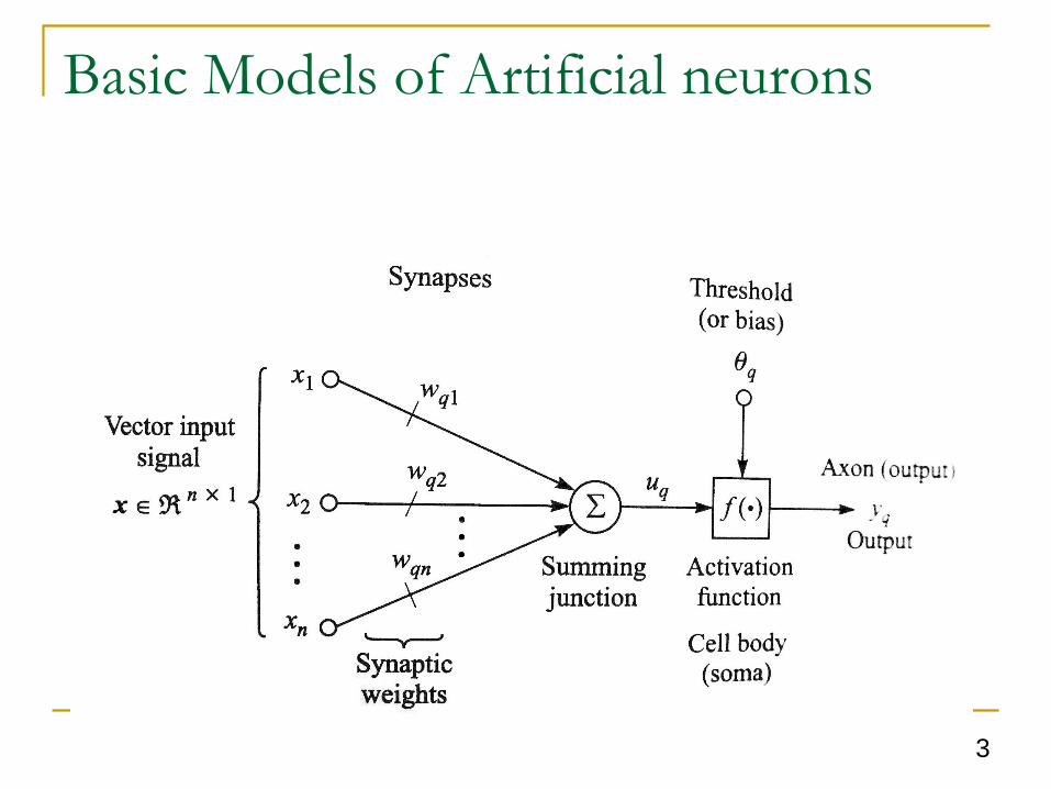
Basic Models of Artificial neurons
An artificial neuron can be referred to as a
processing element, node, or a threshold logic unit.
There are four basic components of a neuron
A set of synapses with associated synaptic weights
A summing device, each input is multiplied by the
associated synaptic weight and then summed.
A activation function, serves to limit the amplitude of the
neuron output.
A threshold function, externally applied and lowers the
cumulative input to the activation function.
3
Basic Models of Artificial neurons

4
Basic Models of Artificial neurons
q
n
j
jqjq
qqqq
T
qnqq
n
j
q
T
jqjq
xwfy
ufvfy
www
xwu
1
1n
21
1
bygiven isneuron theofoutput the
)(
isfunction activation theofoutput the
R,...,, where
iscombiner linear theofoutput the
q
T
q
w
wxxw (2.2)
(2.3)
(2.4)

5
Basic Models of Artificial neurons
The threshold (or bias) is incorporated into the synaptic
weight vector wq for neuron q.

6
Basic Models of Artificial neurons
n
j
jqjq
vfy
q
wv
as written is neuron ofoutput The
as written is potential activation internal effective The
0
x

7
Basic Activation Functions
The activation function, transfer function,
Linear or nonlinear
Linear (identity) activation function
qqlinq vvfy
8
Basic Activation Functions
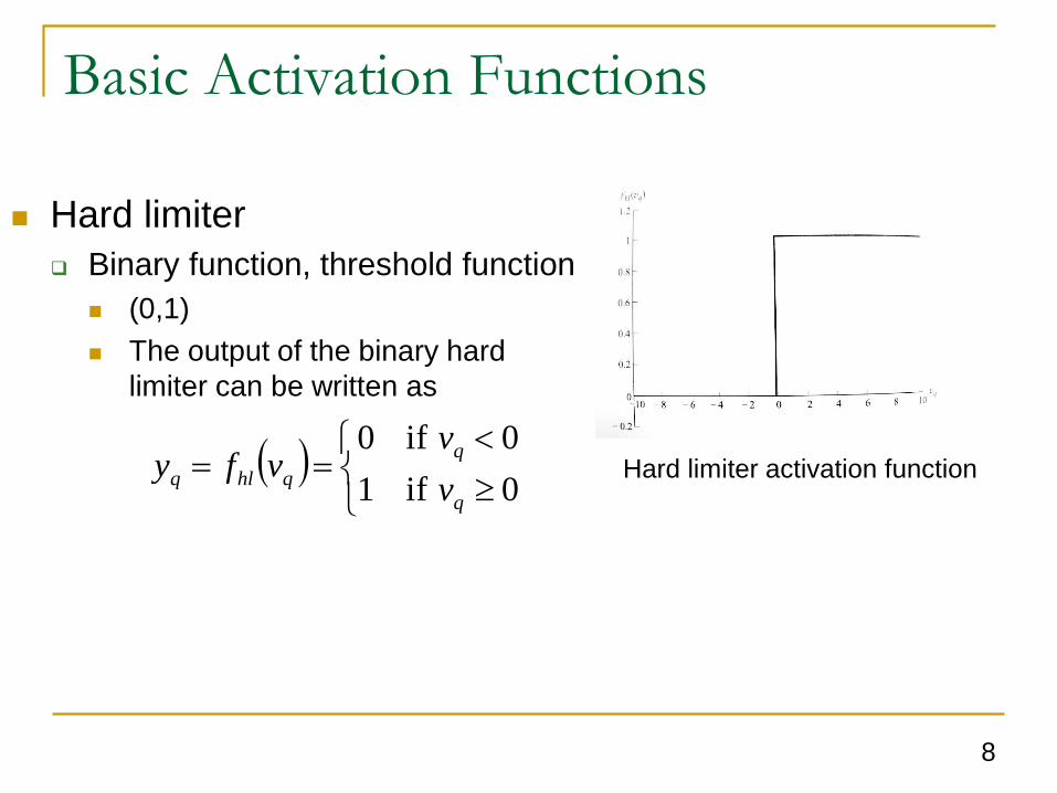
Hard limiter
Binary function, threshold function
(0,1)
The output of the binary hard
limiter can be written as
Hard limiter activation function
0 if1
0 if0
q
q
qhlq v
vvfy

9
Basic Activation Functions
Bipolar, symmetric hard limiter
(-1, 1)
The output of the symmetric
hard limiter can be written as
Sometimes referred to as the
signum (or sign) function.
0 if1
0 if0
0 if1
q
q
q
qshlq
v
v
v
vfy
Symmetric limiter activation function

10
Basic Activation Functions
Saturation linear function,
piecewise linear function
The output of the saturation
linear function is given by
2
1 if1
2
1
2
1- if
2
12
1 if0
q
q
qslq
v
vv
v
vfySaturation linear activation function

11
Basic Activation Functions
Saturation linear function
The output of the symmetric
saturation linear function is
given by
Saturation linear activation function
1 if1
11- if
1 if1
q
q
qsslq
v
vv
v
vfy

12
Basic Activation Functions
Sigmoid function (S-
shaped function)
Binary sigmoid function
The output of the binary
sigmoid function is given
by
qvqbsq
evfy
1
1
Where is the slope parameter of the binary sigmoid function
Binary sigmoid function
Hard limiter has no derivative at the origin, the binary sigmoid is a continuous
and differentiable function.

13
Basic Activation Functions
Sigmoid function (S-shaped
function)
Bipolar sigmoid function,
hyperbolic tangent sigmoid
The output of the Binary sigmoid
function is given by
q
q
v
v
vv
vv
qqhtsqe
e
ee
eevvfy
2
2
1
1tanh

14
Adaline and Madaline
Least-Mean-Square (LMS) Algorithm Widrow-Hoff learning rule
Delta rule
The LMS is an adaptive algorithm that computes adjustments of the neuron synaptic weights.
The algorithm is based on the method of steepest decent.
It adjusts the neuron weights to minimize the mean square error between the inner product of the weight vector with the input vector and the desired output of the neuron.
Adaline (adaptive linear element) A single neuron whose synaptic weights are updated
according to the LMS algorithm.
Madaline (Multiple Adaline)

15
Simple adaptive linear combiner
kxkwkwkxkv TT
inputs
x0=1, wo=b (bias)

16
Simple adaptive linear combiner
The difference between the desired response and
the network response is
The MSE criterion can be written as
Expanding Eq(2.23)
22 )()(2
1)(
2
1)( kkkdEkeEJ T
xww
kkkdkvkdke Txw
)()(2
1)()(
2
1
)()()()(2
1)()()()(
2
1)(
2
2
kkkkdE
kkkEkkkkdEkdEwJ
x
TT
TTT
wCwwp
wxxwwx
(2.22)
(2.23)
(2.24)
(2.25)

17
Simple adaptive linear combiner
Cross correlation vector between the desired
response and the input patterns
Covariance matrix for the input pattern
J(w)的MSE表面有一個最小值(minimum) ,因此計算梯度等於零的權重值
因此,最佳的權重值為
)()( kkdE xp
)()( kkE T
x xxC
0)()(
)(
k
JJ xwCp
w
www
pCw1* x
(2.26)
(2.27)

18
The LMS Algorithm
上式的兩個限制 求解covariance matrix的反矩陣很費時
不適合即時的修正權重,因為在大部分情況,covariance matrix和cross correlation vector無法事先知道。
為避開這些問題,Widow and Hoff提出了LMS algorithm To obtain the optimal values of the synaptic weights when
J(w) is minimum.
Search the error surface using a gradient descent method to find the minimum value.
We can reach the bottom of the error surface by changing the weights in the direction of the negative gradient of the surface.

19
The LMS Algorithm
Typical MSE surface of an adaptive linear combiner

20
The LMS Algorithm
Because the gradient on the surface cannot be computed without knowledge of the input covariance matrix and the cross-correlation vector, these must be estimated during an iterative procedure.
Estimation of the MSE gradient surface can be obtained by taking the gradient of the instantaneous error surface.
The gradient of J(w) approximated as
The learning rule for updating the weights using the steepest descent gradients method as
)()(
)(
2
1)( )(
2
kke
keJ kwww
x
ww
)()()()()()1( kkekJkk w xwwww
(2.28)
(2.29)
Learning rate specifies the magnitude of the update step for the
weights in the negative gradient direction.

21
The LMS Algorithm
If the value of is chosen to be too small, the learning
algorithm will modify the weights slowly and a relatively
large number of iterations will be required.
If the value of is set too large, the learning rule can
become numerically unstable leading to the weights not
converging.
22
The LMS Algorithm
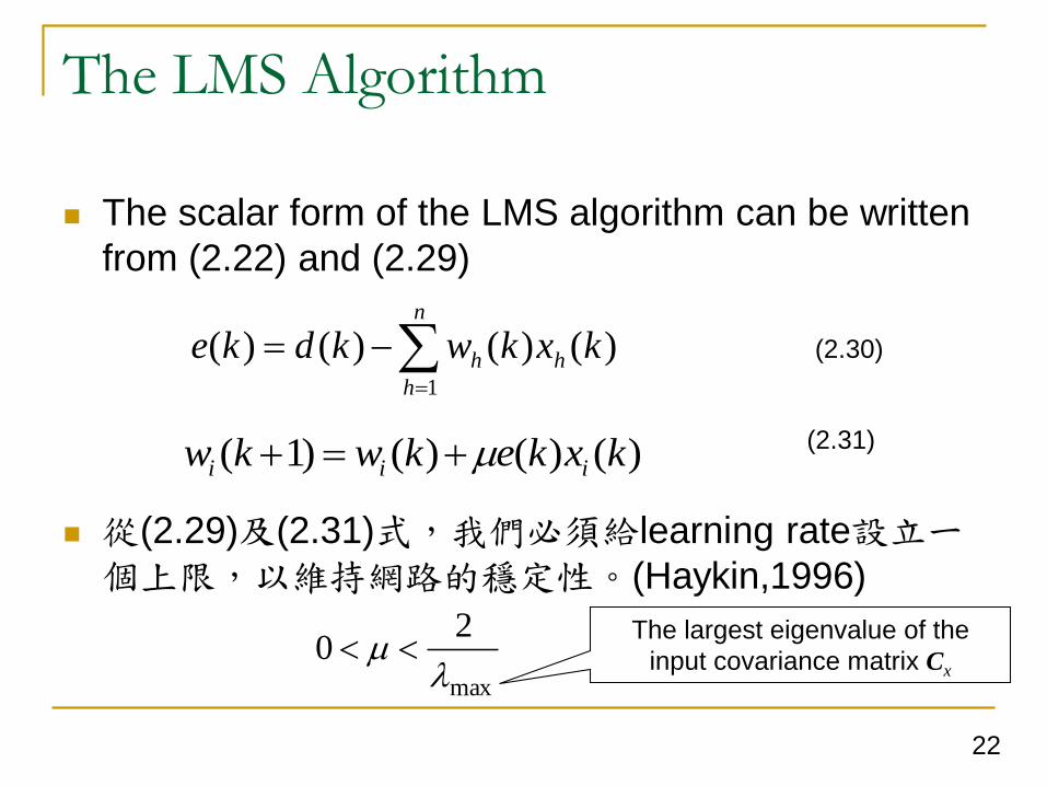
The scalar form of the LMS algorithm can be written
from (2.22) and (2.29)
從(2.29)及(2.31)式,我們必須給learning rate設立一個上限,以維持網路的穩定性。(Haykin,1996)
n
h
hh kxkwkdke1
)()()()(
)()()()1( kxkekwkw iii
(2.30)
(2.31)
max
20
The largest eigenvalue of the
input covariance matrix Cx
23
The LMS Algorithm
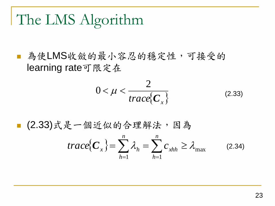
為使LMS收斂的最小容忍的穩定性,可接受的learning rate可限定在
(2.33)式是一個近似的合理解法,因為
xtrace C
20
n
h
n
h
xhhhx ctrace1 1
maxC
(2.33)
(2.34)

24
The LMS Algorithm
從(2.32) 、(2.33)式知道,learning rate的決定,至少得計算輸入樣本的covariance matrix,在實際的應用上是很難達到的。
即使可以得到,這種固定learning rate在結果的精確度上是有問題的。
因此,Robbin’s and Monro’s root-finding algorithm提出了,隨時間變動learning rate的方法。(Stochastic approximation )
where k is a very small constant.
缺點:learning rate減低的速度太快。
kk
k )(
(2.35)
25
The LMS Algorithm
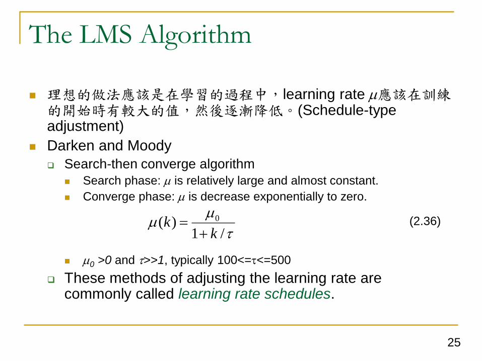
理想的做法應該是在學習的過程中,learning rate 應該在訓練的開始時有較大的值,然後逐漸降低。(Schedule-type adjustment)
Darken and Moody
Search-then converge algorithm
Search phase: is relatively large and almost constant.
Converge phase: is decrease exponentially to zero.
0 >0 and t>>1, typically 100<=t<=500
These methods of adjusting the learning rate are commonly called learning rate schedules.
t
/1)( 0
kk
(2.36)

26
The LMS Algorithm
Adaptive normalization approach (non-schedule-
type)
is adjusted according to the input data every time step
where 0 is a fixed constant.
Stability is guaranteed if 0< 0 <2; the practical range is
0.1<= 0 <=1
2
2
0
)()(
kxk
(2.37)

27
The LMS Algorithm Comparison of two learning rate schedules: stochastic approximation
schedule and the search-then-converge schedule.
Eq.(2.35)
Eq.(2.36)
is a constant

28
Summary of the LMS algorithm
Step 1: set k=1, initialize the synaptic weight vector w(k=1), and
select values for 0 and t.
Step 2: Compute the learning rate parameter
Step 3: Computer the error
Step 4: Update the synaptic weights
Step 5: If convergence is achieved, stop; else set k=k+1, then go to
step 2.
t
/1
0
kk
n
h
hh kxkwkdke1
)()()()(
)()()()()1( kxkekkwkw iii

29
Example 2.1: Parametric system identification
Input data consist of 1000 zero-mean Gaussian random vectors with three components. The bias is set to zero. The variance of the components of x are 5, 1, and 0.5. The assumed linear model is given by b=[1, 0.8, -1]T.
To generate the target values, the 1000 input vectors are used to form a matrix X=[x1x2…x1000], the desired outputs are computed according to d=bTX
The progress of the learning rate parameter as it is adjusted according
to the search-then converge schedule.
bx d
200
1936.09.0
10001000
1
max0
1000
1
t
h
TT
x
XXxxC
The learning process was terminated when
82 102/1 keJ

30
Example 2.1 (cont.)
Parametric system identification: estimating a parameter vector associated with a dynamic model of a system given only input/output data from the system.
The root mean square (RMS) value of the performance measure.

31
Adaline and Madaline
Adaline
It is an adaptive pattern classification network trained by
the LMS algorithm.
x0(k)=1
可調整的bias
或 weight產生bipolar (+1, -1)的輸出,可因activation
function的不同,而有(0,1)的輸出
)()()( kvkdke )()()(~ kykdke

32
Adaline
Linear error
The difference between the desired output and the
output of the linear combiner.
Quantizer error
The difference between the desired output and the
output of the symmetric hard limiter.
)()()( kvkdke
)()()(~ kykdke

33
Adaline
Adaline的訓練過程
輸入向量x必須和對應的desired輸出d,同時餵給Adaline。
神經鍵的權重值w,會根據linear LMS algorithm動態的調整。
Adaline在訓練的過程,並沒有使用到activation function,(activation function只有在測試階段才會使用)
一旦網路的權重經過適當的調整後,可用未經訓練的pattern
來測試Adaline的反應。
如果Adaline的輸出和測試的輸入有很高的正確性時,可稱網路已經generalization。
34
Adaline
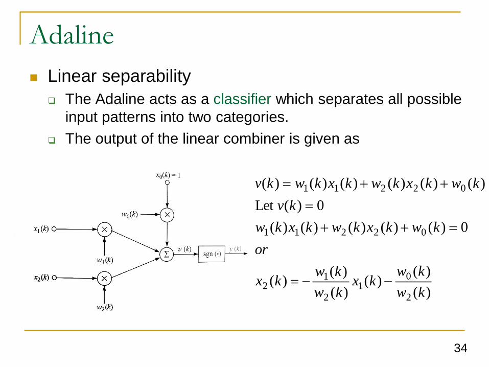
Linear separability
The Adaline acts as a classifier which separates all possible
input patterns into two categories.
The output of the linear combiner is given as
)(
)()(
)(
)()(
0)()()()()(
0)(Let
)()()()()()(
2
01
2
12
02211
02211
kw
kwkx
kw
kwkx
or
kwkxkwkxkw
kv
kwkxkwkxkwkv

35
Adaline
Linear separability of the Adaline
Adaline只能分割線性可分割的patten

36
Adaline
Nonlinear separation problem
若separating boundary
非straight line,Adaline無法分割
Since the boundary is not a straight
line, the Adaline cannot be used to
accomplish this task.

37
Adaline (cont.)
Linear error correction rules
有兩種基本的線性修正規則,可用來動態調整網路的權重值。(網路權重的改變與網路實際輸出和desire輸出的差異有關)
-LMS:same as (2.22) and (2.29) (基於最小化MSE表面)
-LMS: a self-normalizing version of the -LMS learning rule
-LMS演算法是根據最小擾動原則(minimal-disturbance
principle) ,當調整權重以適應新的pattern的同時,對於先前的pattern的反應,應該有最小的影響。
2
2)(
)()()()1(
kx
kxkekwkw (2.46)
)()()()()()1( kxkekwwJkwkw w

38
Adaline (cont.) Consider the change in the error for -LMS
From (2.47)
The choice of a controls stability and speed of convergence, is typically set in the range
-LMS之所以稱為self-normalizing是因為的選擇和網路的輸入大小無關,
keke
kx
kxkxkeke
kekxkx
kxkekwkd
kekxkwkdkekeke
T
TT
T
2
2
2
2
11
ke
ke
11.0
(2.47)
(2.48)

39
Adaline (cont.) Detail comparison of the -LMS and -LMS
From (2.46)
Define normalized desired response and normalized training vector
Eq(2.49) can be rewrote as
222
2
2
2
2
)()()(
)(
)(
)()()()1(
kx
kx
kx
kxkw
kx
kdkw
kx
kxkxkwkdkw
kx
kxkekwkw
T
T
22
,kx
kxkx
kx
kdkd
)()1( kxkxkwkdkwkw T
和-LMS具有相同的型式,所以-LMS表示正規化輸入樣本後的-LMS 。
(2.49)
(2.50-51)
(2.52)
)()()()()()1( kxkekwwJkwkw w

40
Multiple Adaline (Madaline)
單一個Adaline無法解決非線性分割區域的問題。
可使用多個adaline
Multiple adaline
Madaline
Madaline I:single-layer network with single output.
Madaline II:multi-layer network with multiple output.

41
Example of Madaline I network consisting
of three Adalines
May be OR,
AND, and MAJ

42
Two-layer Madaline II architecture

43
Simple Perceptron
Simple perceptron (single-layer perceptron)
Very similar to the Adaline, 由Frank Rosenblatt (1950)提出。
Minsky and Paper發現一個嚴重的限制:perceptron無法解決XOR的問題。
藉由正確的processing layer,可解決XOR問題,或是parity
function的問題。
Simple perceptron和典型的pattern classifier 的maximum-
likelihood Gaussian classifier有關,均可視為線性分類器。
大部分的perceptron的訓練是supervised,也有部分是self-
organizing。

44
Simple Perceptron44
Td
Td
Td
j
jj
xx
www
wxwy
,...,,1
,...,,
1
10
0
1
x
w
xw
(Rosenblatt, 1962)
The perceptron is the basic processing element.

45
What a Perceptron Does?
Regression: y=wx+w0 Classification:y=1(wx+w0>0)
45
ww0
y
x
x0=+1
ww0
y
x
s
w0
y
x
xw
Toy
exp1
1 sigmoid
xwTo

46
Simple Perceptron : K Outputs46
K parallel perceptrons. xj, j = 0, . . . , d are the inputs and yi, i =1,. . .,K
are the outputs. wij is the weight of the connection from input xj to
output yi .
When used for K-class classification problem, there is a post-
processing to choose the maximum, or softmax if we need the
posterior probabilities.

47
K Outputs47
kk
ii
Tii
o
oy
o
exp
exp
xw
Classification:
there are K perceptrons, each of which has a weight vector wi
where wij is the weight from input xj to output yi . W is the K × (d
+ 1) weight matrix of wij
When used for classification, during testing, we
xy
xw
W
Tii
d
j
jiji wxwy 0
1
kk
ii yyC max if choose
Activation
function

48
Simple Perceptron (cont.)
Original Rosenblatt’s perceptron
Binary input, no bias.
Modified perceptron
Bipolar inputs and a bias term
Output y{-1,1}
49
Simple Perceptron (cont.)
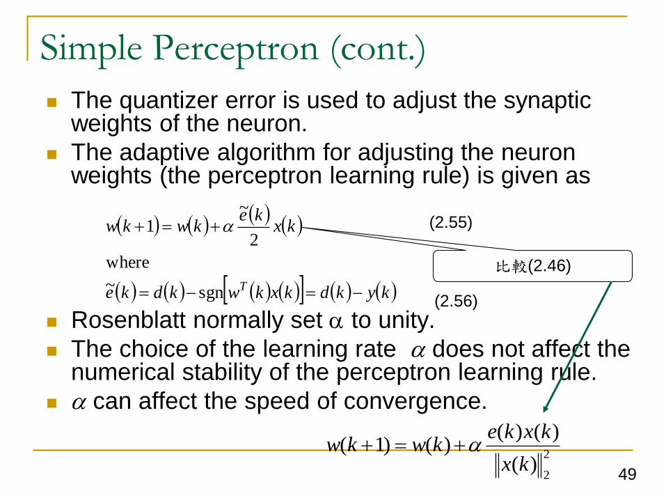
The quantizer error is used to adjust the synaptic weights of the neuron.
The adaptive algorithm for adjusting the neuron weights (the perceptron learning rule) is given as
Rosenblatt normally set to unity.
The choice of the learning rate does not affect the numerical stability of the perceptron learning rule.
can affect the speed of convergence.
kykdkxkwkdke
kxke
kwkw
T
sgn~
where
2
~1 (2.55)
(2.56)
比較(2.46)
2
2)(
)()()()1(
kx
kxkekwkw

50
Simple Perceptron (cont.)
The perceptron learning rule is considered a nonlinear
algorithm.
The perceptron learning rule performs the update of the
weights until all the input patterns are classified correctly.
The quantizer error will be zero for all training pattern inputs, and
no weight adjustments will occur.
The weights are not guaranteed to be optimal.

51
Simple Perceptron with a Sigmoid Activation Function
The learning rule is based on the method of steepest
descent and attempts to minimize an instantaneous
performance function.

52
Simple Perceptron with a Sigmoid Activation Function (cont.)
學習演算法可由MSE推導獲得
The instantaneous performance function to be
minimized is given as
kykdke
keEJ
qqq
~ where
~
2
1 2w
T
qqqq
qqqq
kwkxfkvfky
kykykdkd
kykdkeJ
where
22
1
2
1~
2
1
22
22w
(2.61)
(2.60)
(2.59)

53
Simple Perceptron with a Sigmoid Activation
Function (cont.)
假設 activation function為hyperbolic tangent
sigmoid,因此,神經元的輸出可表示成
根據(2.15)式對hyperbolic tangent sigmoid函數的微分
採用steepest descent的discrete-time learning rule
kvkvfky qqhtsq tanh
kvfkvfkvg qqq
21'
qwqq Jkk www 1
(參考2.29式)
(2.64)
(2.63)
(2.62)
)()()()()()1( kxkekJkk w wwww
qbsqbs
v
v
q
qbs
qbs vfvfe
e
dv
vdfvg
q
q
11
2

54
Simple Perceptron with a Sigmoid Activation
Function (cont.)
計算(2.64)式的梯度(gradient)
以(2.63)式代入(2.65)式
採用(2.66)式的gradient,則discrete-time learning rule for simple
perceptron 可寫成
kxkvfke
kxkvfkvfkd
kxkvfkvfkxkvfkdJ
qqq
qqqqqw
~
'
''
w
kxkyke
kxkvfkeJ
qqqw
2
2
1~
1~
w
kxkykekk qqqq
21~1 ww
(2.65)
(2.66)
(2.67)

55
Simple Perceptron with a Sigmoid Activation
Function (cont.)
(2.67)式可改寫成scalar form
其中
(2.68) 、(2.69)和 (2.70)為backpropagation training algorithm的標準形式。
kxkykekwkw jqqqjqj
21~1
n
j
qqjjqq
qqq
kwkxfkvfky
kykdke
1
~
(2.70)
(2.69)
(2.68)

56
Example 2.2
Applied the architecture of Figure 2.30 to learn character “E”
The character image consists of 5x5 array, 25 pixel (column major)
The learning rule is Eq.(2.67), with =1, =0.25
The desired neuron response d=0.5, error goal 10-8.
The initial weights of the neuron were randomized.
After 39 training pattern, the actual neuron output y=0.50009 (see Fig.
2.32)

57
Example 2.2 (cont.)
The single neuron cannot
correct for a noisy input.
For Fig. 2.31 (b), y=0.5204
For Fig. 2.31 (c), y=0.6805
To compensate for noisy
Multi-layer perceptron
Hopfield associative
memory.
58
Feedforward Multilayer Perceptron
The multilayer perceptron is an artificial neural
network structure and is a nonparametric estimator
that can be used for classification and regression.
Multilayer perceptron (MLP)
The branches can only broadcast information in one direction.
Synaptic weight can be adjusted according to a defined
learning rule.
h-p-m feedforward MLP neural network.
In general there can be any number of hidden layers in the
architecture; however, from a practical perspective, only one
or two hidden layer are used.

59
Feedforward Multilayer Perceptron (cont.)

60
Feedforward Multilayer Perceptron (cont.)
The first layer has the weight matrix
The second layer has the weight matrix
The third layer has the weight matrix
Define a diagonal nonlinear operator matrix
nh
jiwW )1()1(
hp
rjwW )2()2(
pm
srwW )3()3(
)()()( ,...,, fffdiagf (2.71)

61
Feedforward Multilayer Perceptron (cont.)
The output of the first layer can be written as
The output of the second layer can be written as
The output of the third layer can be written as
將(2.72)代入(2.73) ,再代入(2.74)可得最後的輸出為
xWvx)1()1()1()1(
1 ffout
1
)2()2()2()2(
2 outout ff xWvx
2
)3()3()3()3(
3 outout ff xWvx
(2.72)
(2.73)
(2.74)
xWWW)1()1()2()2()3()3( fffy (2.75)
The synaptic weights are fixed, a training process must be carried out a priori
To properly adjust the weights.

62
Overview of Basic Learning Rules for a Single Neuron
Generalized LMS Learning Rule
定義一個需最小化的performance function (energy function)
其中, ||w||2為向量w的Euclidean norm
Y(.)為任何可微分的函數,e is the linear error。
2
22)( ww
e
xwTde
Desired output
Weight vector Input vector
(2.76)
(2.77)

63
Generalized LMS Learning Rule (cont.) 採用最陡坡降法(steepest descent approach) ,可獲得
general LMS algorithm。
Continuous-time learning rule(可視為向量的微分)
Discrete-time learning rule
If Y(t)=1/2t2, and Y ’(t)=g(t)=t, then (2.81) is written as
wx
ww
)(
)(
eg
dt
dw
)()()()(
)()()1(
kkegk
kk w
wxw
www
Learning rate Leakage factor
(2.78)
(2.79)
(2.82)
(2. 81)
wxwxwxw
eeedt
d(2.83)

64
Generalized LMS Learning Rule (cont.)
Leaky LMS algorithm (0<=<1)
Standard LMS algorithm (=0), (the same as Eq.2.29)
The scalar form of standard LMS algorithm
)()()()1(
)()()()()1(
kkek
kkkekk
xw
wxww
)()()()1( kkekk xww
(2.84)
(2.85)
n
j
jj
jjj
kxkwkdke
nj
kxkekwkw
1
)()()()(
,...,2,1,0for
)()()()1( (2.86)
65
Generalized LMS Learning Rule (cont.)
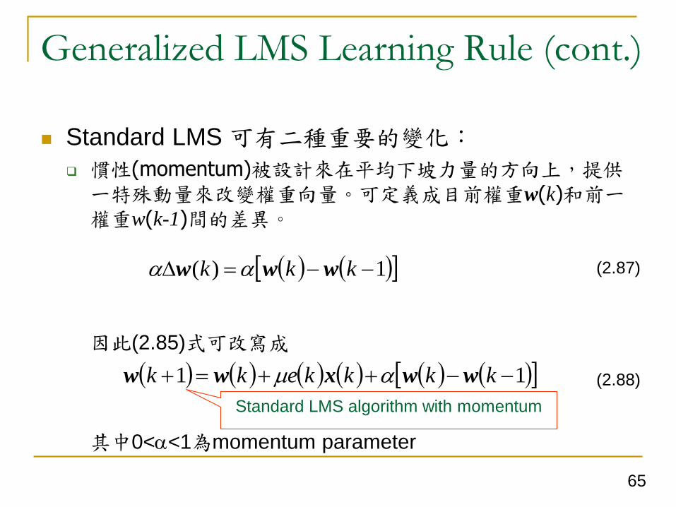
Standard LMS 可有二種重要的變化:
慣性(momentum)被設計來在平均下坡力量的方向上,提供一特殊動量來改變權重向量。可定義成目前權重w(k)和前一權重w(k-1)間的差異。
因此(2.85)式可改寫成
其中0<<1為momentum parameter
1)( kkk www
11 kkkkekk wwxww
(2.87)
(2.88)
Standard LMS algorithm with momentum
66
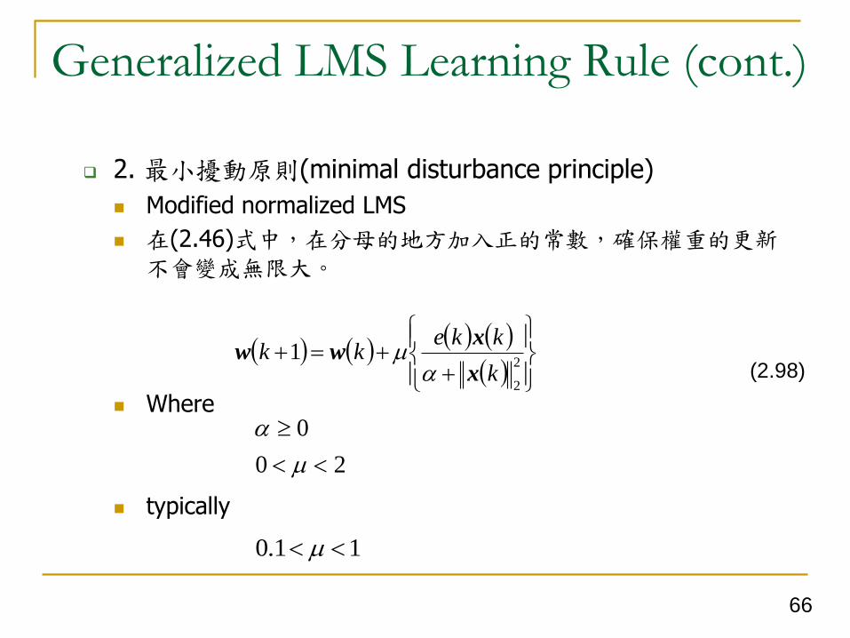
Generalized LMS Learning Rule (cont.)
2. 最小擾動原則(minimal disturbance principle)
Modified normalized LMS
在(2.46)式中,在分母的地方加入正的常數,確保權重的更新不會變成無限大。
Where
typically
2
2
1k
kkekk
x
xww
(2.98)
20
0
11.0

67
Example 2.3
The same as Example
2.1,但使用不同的LMS
algorithm。
Use the same
Initial weight vector
Initial learning rate
Termination criterion

68
Overview of basic learning rules for a
single neuron (cont.)
Standard Perceptron Learning Rule
可由minimizing the MSE criterion來推導獲得
其中
神經元的輸出
採用steepest descent approach, the continuous-time
learning rule is given by
2
2
1)( ew
yde
)()( vfxwfy T
)(wdt
dww
(2.132)
(2.133)
(2.134)

69
Overview of basic learning rules for a
single neuron (cont.)
則(2.132)式的gradient可得
x
xdv
vdfe
xdv
vdfvd
xdv
vdfvx
dv
vdfdww
)(
)()(
)()(
)()(
)()(')(
vegvefdv
vdfe
其中
(2.135)
(2.136)

70
Overview of basic learning rules for a
single neuron (cont.)
使用(2.134), (2.135)和(2.136)式,the continuous-time
standard perceptron learning rule for a single neuron as
(2.137)式可改寫成discrete-time形式
The scalar form of (2.138) can be written as
xdt
dw
)()()()1( kxkkwkw
)()()()1( kxkkwkw jjj
(2.137)
(2.138)
(2.139)
71
Overview of basic learning rules for a
single neuron (cont.)
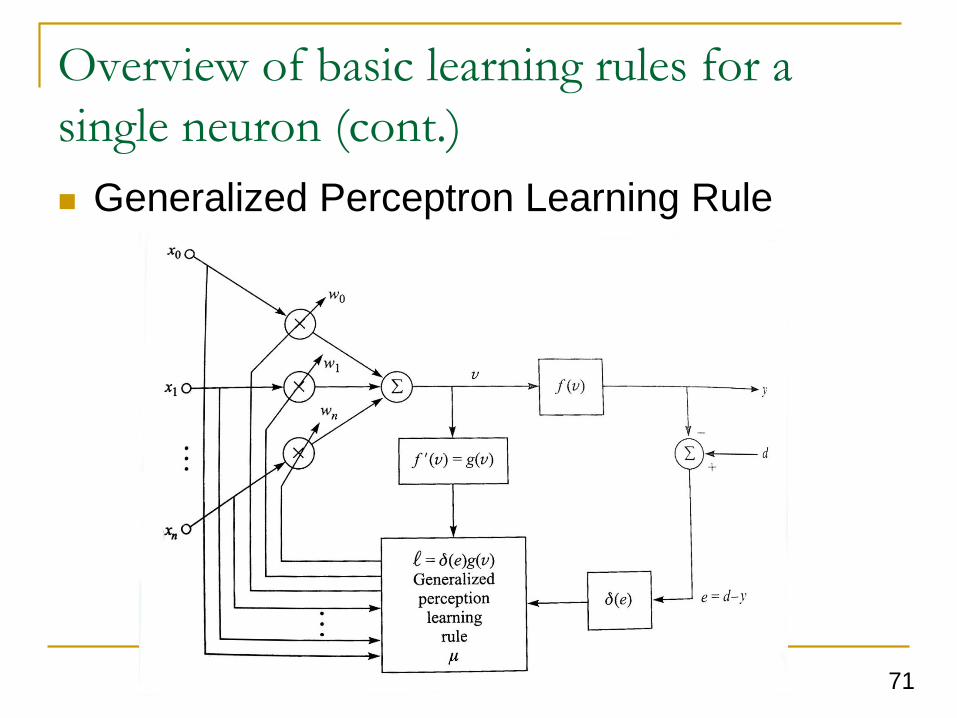
Generalized Perceptron Learning Rule

72
Overview of basic learning rules for a
single neuron (cont.)
Generalized Perceptron Learning Rule
When the energy function is not defined to be the MSE
criterion, we can define a general energy function as
其中.為可微函數。如果.1/2 e2 則變成standard
perceptron learning rule.
其中
)()()( ydew
w
v
v
y
y
e
eww
)(
)()(')(
eee
e
)(vfxwfy T
(2.141)
(2.142)
(2.143)
(2.140)

73
Overview of basic learning rules for a
single neuron (cont.) f(.) is a differentiable function, and
(2.141) can be written as
The continuous-time general perceptron learning rule is given as
If we define the learning signal as
(2.146) can be written as
)()(')()(
vgvfdv
vdf
dv
vdy
xvgeww )()()(
xvgedt
dw)()(
)()( vge
xdt
dw
(2.144)
(2.145)
(2.146)
(2.147)
(2.148)

74
Overview of basic learning rules for a
single neuron (cont.)
Discrete-time form
Discrete scalar form
)()()()1( kxkkwkw
)()()()1( kxkkwkw jjj
(2.149)
(2.150)

75
Data Preprocessing
The performance of a neural network is strongly dependent on the preprocessing that is performed on the training data.
Scaling
The training data can be amplitude-scaled in two ways The value of the pattern lie between -1 and 1.
The value of the pattern lie between 0 and 1.
Referred to as min/max scaling.
MATLAB: premnmx

76
Data Preprocessing (cont.)
Another scaling process
Mean centering
如果用來training的data包含有biases時。
Variance scaling
如果用來training的data具有不同的單位時。
假設輸入向量以行方向排列成矩陣
目標向量也以行方向排列成矩陣
Mean centering
計算矩陣A、C中每一列的 mean value
將矩陣A、C中的每個元素,減去該對應的mean value。
Variance scaling
計算矩陣A、C中每一列的 standard deviation.
將矩陣A、C中的每個元素,除以該對應的standard deviation 。
mnA mpC

77
Data Preprocessing (cont.)
Transformations
The feature of certain “raw” signals are used fro training
inputs provide better results than the raw signals.
A front-end feature extractor can be used to discern salient
or distinguishing characteristics of the data.
Four transform methods:
Fourier Transform
Principal-Component Analysis
Partial Least-Squares Regression
Wavelets and Wavelet Transforms

78
Data Preprocessing (cont.)
Fourier Transform
The FFT can be used to extract the import
features of the data, and then these dominant
characteristic features can be used to train the
neural network.

79
Data Preprocessing (cont.)三個具有相同波形,不同相位的信號,每個信號具有1024個取樣點。

80
Data Preprocessing (cont.)
在FFT magnitude response上,具有相同magnitude response ,而且只需16個magnitude取樣即可。
三個具有相同波形,不同相位的信號,在FFT的相位上則有所不同。

81
Data Preprocessing (cont.)
Principal-Component Analysis
PCA can be used to “compress” the input training
data set, reduce the dimension of the inputs.
By determining the important features of the data
according to an assessment of the variance of the
data.
In MATLAB, prepca is provided to perform PCA
on the training data

82
Data Preprocessing (cont.) Given a set of training data
where assumed that m>>n,n denote the dimension of the input training patternsm denote the number of training pattern.
Using PCA, an “optimal” orthogonal transformation matrix can be determined
where h<<n (the degree of dimension reduction)
The dimension of the input vectors can be reduced according to the transformation
where Ar is the reduced-dimension set of training patterns.The columns of Ar are the principal components for each of the inputs from A
mnA
nh
pcaW
AWA pcar
mh
rA
(2.151)
83
Data Preprocessing (cont.)
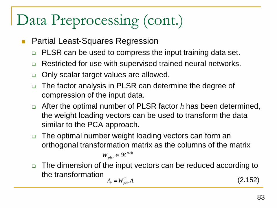
Partial Least-Squares Regression
PLSR can be used to compress the input training data set.
Restricted for use with supervised trained neural networks.
Only scalar target values are allowed.
The factor analysis in PLSR can determine the degree of
compression of the input data.
After the optimal number of PLSR factor h has been determined,
the weight loading vectors can be used to transform the data
similar to the PCA approach.
The optimal number weight loading vectors can form an
orthogonal transformation matrix as the columns of the matrix
The dimension of the input vectors can be reduced according to
the transformation
hn
plsrW
AWA T
plsrr (2.152)

84
Data Preprocessing (cont.)
PCA and PLSR orthogonal transformation vectors used for data compression
PLSR使用輸入資料與目標資料來產生orthogonal transformation Wplsr的weight loading vector
85
Data Preprocessing (cont.)
Wavelets and Wavelet Transforms
A wave is an oscillating function of time.
Fourier analysis is used for analyzing waves
Certain function can be expanded in terms of sinusoidal waves.
How much of each frequency component is required to synthesize the signal.
Very useful for periodic, time-invariant, stationary signal analysis.
A wavelet can be considered as a small wave, whose energy is concentrated.
Useful for analyzing signals that are time-varying, transient, nonstationary.
To allow for simultaneous time and frequency analysis.
Wavelets are local waves.
The wavelet transform can provide a time-frequency description of signals and can be used to compress data for training neural network.