gearbox+ +rossir24 0017
TRANSCRIPT

8/6/2019 Gearbox+ +Rossir24 0017
http://slidepdf.com/reader/full/gearbox-rossir24-0017 1/91
Condition Monitoring System in WindTurbine Gearbox
MICHELE LUCENTE
Master’s Degree ProjectStockholm, Sweden 2008
8/6/2019 Gearbox+ +Rossir24 0017
http://slidepdf.com/reader/full/gearbox-rossir24-0017 2/91
CONDITIONMONITORINGSYSTEM INWINDTURBINEGEARBOX
Master Thesisby Michele Lucente
Master Thesis written at KTH, Royal Institute of Technology, April 2008,School of Electrical Engineering
Supervisor: Associate Professor Lina Bertling,KTH School of Electrical Engineering,Examiner: Associate Professor Lina Bertling,KTH School of Electrical Engineering,Assistant Supervisor: Ph.D. student Francois Besnard,KTH School of Electrical Engineering
XR-EE-ETK 2008:004

8/6/2019 Gearbox+ +Rossir24 0017
http://slidepdf.com/reader/full/gearbox-rossir24-0017 3/91

8/6/2019 Gearbox+ +Rossir24 0017
http://slidepdf.com/reader/full/gearbox-rossir24-0017 4/91
Abstract
This master thesis describes the use of Condition Monitoring Systems and its appli-cation in maintenance optimization for wind turbines. The focus is on the gearbox,
one of the most critical compenents in terms of high failure rates and long meandown time. Two different models for cost optimal maintenance are presented anddiscussed. The thesis include also a basic description of the gearbox and its sub-components togheter with the most common techniques for condition monitoring.
iii

8/6/2019 Gearbox+ +Rossir24 0017
http://slidepdf.com/reader/full/gearbox-rossir24-0017 5/91

8/6/2019 Gearbox+ +Rossir24 0017
http://slidepdf.com/reader/full/gearbox-rossir24-0017 6/91
Acknowledgements
I would like to thank my supervisor and examiner at the Royal Institute of Tech-nology Lina Bertling for taking her time and giving me support and help during the
difcult times of the project work.Furthermore, I would also like to thank the Ph.D. student François Besnard forhis advices involving technical issues and the report itself.
Sincerely, Michele LucenteStockholm, April 2008
v

8/6/2019 Gearbox+ +Rossir24 0017
http://slidepdf.com/reader/full/gearbox-rossir24-0017 7/91

8/6/2019 Gearbox+ +Rossir24 0017
http://slidepdf.com/reader/full/gearbox-rossir24-0017 8/91
Contents
Abstract iii
Acknowledgements v
1 Introduction 31.1 Problem Background . . . . . . . . . . . . . . . . . . . . . . . . 31.2 Previous Work in RCAM . . . . . . . . . . . . . . . . . . . . . . 31.3 Objective . . . . . . . . . . . . . . . . . . . . . . . . . . . . . . 51.4 Thesis overview . . . . . . . . . . . . . . . . . . . . . . . . . . . 6
2 Maintenance Theory 72.1 Condition Based Maintenance . . . . . . . . . . . . . . . . . . . 92.2 Remaining Useful Life . . . . . . . . . . . . . . . . . . . . . . . 102.3 Optimizing Condition Based Maintenance . . . . . . . . . . . . . 122.4 Condition Based Maintenance Models . . . . . . . . . . . . . . . 132.5 General Framework . . . . . . . . . . . . . . . . . . . . . . . . . 152.6 Failure Modes and Criticality Analysis . . . . . . . . . . . . . . . 19
3 System Description: The Gearbox 273.1 Gears . . . . . . . . . . . . . . . . . . . . . . . . . . . . . . . . 293.2 Lubrication and Cooling . . . . . . . . . . . . . . . . . . . . . . 323.3 Operation and Maintenance Activities . . . . . . . . . . . . . . . 333.4 Costs for Operation and Maintenance . . . . . . . . . . . . . . . 343.5 Failure Modes Analysis in Gears . . . . . . . . . . . . . . . . . . 37
4 Condition Monitoring Systems in Wind Turbine’s Gearbox 434.1 Vibration Analysis Techniques . . . . . . . . . . . . . . . . . . . 454.2 Lubricating Oil Analysis . . . . . . . . . . . . . . . . . . . . . . 484.3 SCADA - Supervisory Control And Data Acquisition . . . . . . . 51
5 Including CMS data in Maintenance Modeling 535.1 Basic Concepts . . . . . . . . . . . . . . . . . . . . . . . . . . . 535.2 Proportional Hazards Model . . . . . . . . . . . . . . . . . . . . 565.3 Model Building . . . . . . . . . . . . . . . . . . . . . . . . . . . 58
vii
8/6/2019 Gearbox+ +Rossir24 0017
http://slidepdf.com/reader/full/gearbox-rossir24-0017 9/91
5.4 Cost model and optimization . . . . . . . . . . . . . . . . . . . . 59
5.5 Possible application on the wind turbine gearbox . . . . . . . . . 615.6 Competing risks . . . . . . . . . . . . . . . . . . . . . . . . . . 615.7 Remarks on the use of PHM . . . . . . . . . . . . . . . . . . . . 63
6 Routines for Data Collection 656.1 The OREDA project . . . . . . . . . . . . . . . . . . . . . . . . 656.2 Data Quality . . . . . . . . . . . . . . . . . . . . . . . . . . . . . 676.3 Boundaries of Equipment . . . . . . . . . . . . . . . . . . . . . . 686.4 Taxonomy . . . . . . . . . . . . . . . . . . . . . . . . . . . . . . 68
7 Closure 717.1 Conclusions . . . . . . . . . . . . . . . . . . . . . . . . . . . . . 717.2 Future work . . . . . . . . . . . . . . . . . . . . . . . . . . . . . 72
A Appendix: Partial Likelihood for PHM parameters estimation 73A.1 Estimation method for regression coefcients . . . . . . . . . . . 73A.2 Estimation method for the baseline hazard function . . . . . . . . 75
viii

8/6/2019 Gearbox+ +Rossir24 0017
http://slidepdf.com/reader/full/gearbox-rossir24-0017 10/91
Abbreviations
CBM Condition Based Maintenance
CM Corrective Maintenance
CMMS Computerized Maintenance Management System
FMECA Failure Mode and Criticality Analysis
ECN Energy Center of Netherlands
ISET Institut fur Solare Energieversorgungstechnk
MTTF Mean Time To Failure
OREDA Offshore Reliability Database
PM Preventive MaintenancePHM Proportional Hazards Model
RCM Reliability Centered Maintenance
RUL Remaining Useful Life
SCADA Supervisory Control And Data Acquisition
1

8/6/2019 Gearbox+ +Rossir24 0017
http://slidepdf.com/reader/full/gearbox-rossir24-0017 11/91

8/6/2019 Gearbox+ +Rossir24 0017
http://slidepdf.com/reader/full/gearbox-rossir24-0017 12/91
Chapter 1
Introduction
1.1 Problem Background
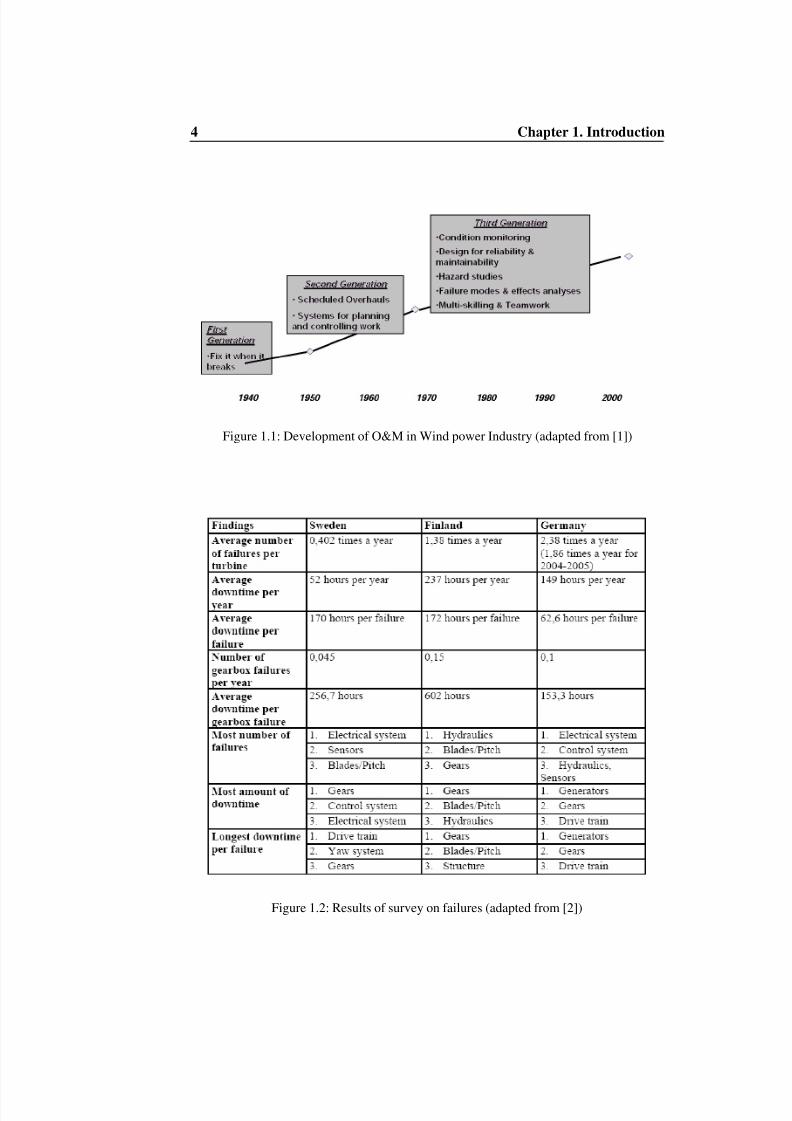
Due to the high costs for operation and maintenance in the wind power industry,particularly on offshore applications, many utility companies and wind turbinesowners are focusing on costs reduction for operation and maintenance. In order toachieve this result it is fundamental to lower part of the corrective maintenance byincreasing preventive maintenance tasks. As shown in Figure 1.1, the state-of-artmaintenance approach in wind power industry is characterized by employment of Reliability Centred Maintenance (RCM) and Condition Monitoring Systems.
The condition monitoring techniques have been used in various industries fordecades, but optimal use of these would in any case require a good understand-ing of the actual component being monitored, and the criticality of this component.Generally the challengewhen it comes to optimizationwould be to determinewhento do inspection, and at what degradation levels we should improve, or renew thecomponent under consideration. In such a discussion we need to take into accountboth the failure progression models, and the cost models.In other terms, the fol-lowing question should be answered: "How should the Condition Monitoring beused in relation with maintenance planning and operation?"
1.2 Previous Work in RCAM
In a Master thesis within RCAM group [2], a surveyon statistics for the wind powerindustry in Sweden, Finland and Germany has been carried out. Findings of theinvestigation, illustrated in Figure 1.2 , has highlighted how failures in gearboxesare critical with respect of failure rates and mean down time. Another importantnding in the thesis is that bigger sized wind turbines have an higher frequency of failures compared with smaller and older turbines
3
8/6/2019 Gearbox+ +Rossir24 0017
http://slidepdf.com/reader/full/gearbox-rossir24-0017 13/91
4 Chapter 1. Introduction
Figure 1.1: Development of O&M in Wind power Industry (adapted from [1])
Figure 1.2: Results of survey on failures (adapted from [2])
8/6/2019 Gearbox+ +Rossir24 0017
http://slidepdf.com/reader/full/gearbox-rossir24-0017 14/91
1.3. Objective 5
Similar results are also presented in other reports available in public literature
([3], [4], [5],[6]).Naturally, criticality of the gearbox increases dramatically in thecase of offshore wind turbines.
Maintenance operations in Offshore wind farms are complex and in average theycan take much longer than an equivalent maintenance action on onshore as they arehighly dependent by weather and sea condition, and by the typology of equipmentneeded (vessel, cranes, etc.). The question to ask when evaluating any of thesecondition monitoring systems is whether the cost of installing and commissioningthese systems is justied throughout the life time of the wind turbine. In otherterms, it is important to determine if the investment costs for installing and runningthe condition monitoring systems are justied by a reduction of costs for mainte-nance. One possible approach to perform a Life Cycle Costs Analysis: this is whathas been done in [7], by calculating life cycle cost for different levels of preventivemaintenance throughout the average life time of a wind turbine (20 years). Resultsof the work has shown how increasing preventive maintenance can make the in-vestment in a CMS protable. The situation becomes even more positive when anentire wind farm is considered rather than single Wind turbine [7].
In general, a CMS is the only a tool acquire information and measures aboutspecic parameters in the wind turbine. If these data are not used as input fordeveloping a condition based maintenance programme, a CMS would never turnout to be benecial both in terms of maintenance efciency and costs.
1.3 Objective
The main objective for the present work is to investigate, with focus on the Gear-box, how CMS can be utilized in maintenance planning and what type of modelscan be employed in order to include CMS data. The work has been divided in thefollowing sub-tasks:
1. Description of how the gearbox works
2. Possible failures and causes and mechanisms leading to failure (FMEA)
3. How could the condition of the gearbox be measured
4. How the gearbox is maintained with focus on preventive maintenance andhow failures can be reduced or postponed

8/6/2019 Gearbox+ +Rossir24 0017
http://slidepdf.com/reader/full/gearbox-rossir24-0017 15/91
6 Chapter 1. Introduction
1.4 Thesis overview
• Chapter 1 - Introduction Problem formulation, background for the thesis aswell as the previous works related with the thesis’s topic. Objectives for thepresent work are also established.
• Chapter 2 - Maintenance Theory Different strategies for maintenance plan-ning, their main features, pros and cons. Brief description of RCM andRCAM approach. Decision framework for condition based maintenance andexamples of modeling for cost optimal maintenance.
• Chapter 3 - System Description Description of the gearbox and its subcom-ponents is given. Terminology used for gears is introduced and differenttypologies of gearboxes employed in the wind industry are illustrated. Inthis chapter, an overview of how gears can fail is given and it is based oncurrent standards applied by gears manufacturers.
• Chapter 4 - Condition Monitoring Systems in the wind turbine gearbox De-scription of condition monitoring techniques for wind power application. Vi-bration, Oil analysis and brief discussion of supervisory and control dataacquisition system (SCADA).
• Chapter 5 - Including CMS data in Maintenance Modeling The focus in thischapter is on the use of predictive maintenance for a wind turbine’s gearboxand how information obtained from Condition Monitoring Systems could beemployed to plan maintenance operations. The proportional hazard modelis intruduced and one possible application is presented. criticality on thesystem, carry out corrective actions. FMECA is probably the most usedmethodology to achieve such result. A description of how to perform theanalysis is presented in this chapter.
• Chapter 6 Routines for data collection An important role in any type of re-liability analysis is played by the reliability data, which mainly consist infailure times. wind power industry is lacking any standardized data collec-tion. The Collection and exchange of reliability and maintenance data forequipment is illustrated by referring to the main international standard IEC14224. The OREDA database is also briey discussed.
• Chapter 7 Closure Conclusions and suggested future work.

8/6/2019 Gearbox+ +Rossir24 0017
http://slidepdf.com/reader/full/gearbox-rossir24-0017 16/91
Chapter 2
Maintenance Theory
Maintenance may be divided into two main categories: corrective and preventive.Preventive maintenance is carried out at predetermined intervals or according toprescribed criteria and intended to reduce the probability of failure or the degra-dation of the functioning of an item. Corrective maintenance is performed after afault in the item has been detected and it is also known asRun to Failure strategy(IEC-61300). The function of maintenance is to assure that the system is able toperform the function it is designed for. In order to achieve this objective differentaspects needs to be taken into account such as:
• Inspection frequency (part of preventive maintenance policy)
• Overhauls intervals (part of preventive maintenance policy)
• Replacement Rules for components
• Management of Spare Parts
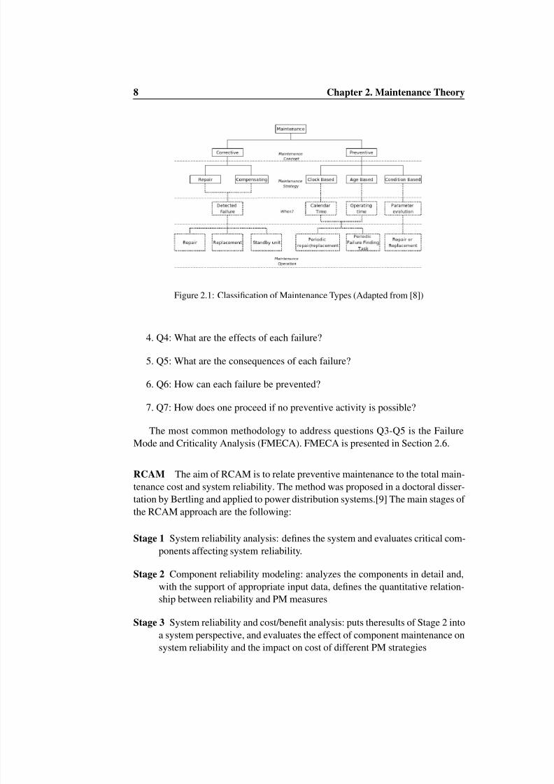
Figure 2.1 sums up the different policies for maintenance for industrial ap-plications. Preventive Maintenance tasks can be performed within periodic timeintervals (either based on operating time of the equipment or calendar time) orbased on measurement of one or more variables that are correlated to a degradationof the system (Condition Based Maintenance).
RCM The RCM philosophy for preventive maintenance is “A preventive task isworth doing if it deals successfully with the consequences of failure which it ismeant to prevent”( RCM process can also be formulated into seven questions, afterthe system items to be analyzed are identied. According to Maubray (1991), theRCM process may be resumed with the following 7 questions:
1. Q1: What are the functions and performances required?
2. Q2: In what ways can each function fail?
3. Q3: What causes each functional failure?
7
8/6/2019 Gearbox+ +Rossir24 0017
http://slidepdf.com/reader/full/gearbox-rossir24-0017 17/91
8 Chapter 2. Maintenance Theory
Figure 2.1: Classication of Maintenance Types (Adapted from [8])
4. Q4: What are the effects of each failure?
5. Q5: What are the consequences of each failure?
6. Q6: How can each failure be prevented?
7. Q7: How does one proceed if no preventive activity is possible?The most common methodology to address questions Q3-Q5 is the Failure
Mode and Criticality Analysis (FMECA). FMECA is presented in Section 2.6.
RCAM The aim of RCAM is to relate preventive maintenance to the total main-tenance cost and system reliability. The method was proposed in a doctoral disser-tation by Bertling and applied to power distribution systems.[9] The main stages of the RCAM approach are the following:
Stage 1 System reliability analysis: denes the system and evaluates critical com-ponents affecting system reliability.
Stage 2 Component reliability modeling: analyzes the components in detail and,with the support of appropriate input data, denes the quantitative relation-ship between reliability and PM measures
Stage 3 System reliability and cost/benet analysis: puts theresults of Stage 2 intoa system perspective, and evaluates the effect of component maintenance onsystem reliability and the impact on cost of different PM strategies

8/6/2019 Gearbox+ +Rossir24 0017
http://slidepdf.com/reader/full/gearbox-rossir24-0017 18/91
2.1. Condition Based Maintenance 9
Figure 2.2: The three main steps in RCM (Adapted from [9])
2.1 Condition Based Maintenance
Condition based maintenance can then be applied to determine if the oil needs tobe changed after say 4 years (calendar-based) or maybe after 7 years (conditionbased). This could save one oil change within the turbine lifetime. So called"safe life components" such as rotor blades for instance are designed for a lifetimelonger than that of the turbinelifetime. If such components are replaced duringthe lifetime, the failure cause is usually not wear but e.g. too high loading, poormanufacturing, or unforeseen conditions.
Furthermore it should be noted that condition based is feasible if:
1. the design life of the component is shorter than that of the entire turbine
2. it is clear that wear indeed is the cause of failure. Gearbox oil for instancewill be replaced several times during the turbine lifetime.
Preventive maintenance involves the repair actions, replacement, and maintenanceof equipment in order to avoid unexpected failure during use. The aim of a PM
programme is to minimize both the costs for inspections and repairs and the costsdue to equipment downtime (measured in terms of production losses).
The traditional approach in preventive maintenance is based on the use of statis-tical and reliability analysis (i.e, failure rates, MTTF) in order to minimize the totalcost by establishing xed or variable ”optimal” PM intervals at which to replace orto overhaul the system.
CBM indicates instead a preventive maintenance programmewhere theapproachinvolves the use of CMS that continuously monitor equipment condition in order

8/6/2019 Gearbox+ +Rossir24 0017
http://slidepdf.com/reader/full/gearbox-rossir24-0017 19/91
10 Chapter 2. Maintenance Theory
to predict when machine failure will occur. Under Condition-Based maintenance,
intervals between maintenance operations are no longer xed, but are performedonly when required. A CBM program consists of three key steps [10]:
1. Data acquisition step , to obtain data relevant to system health (informationcollecting )
2. Data processing step to handle and analyze data for better understanding andinterpretation. (Diagnosis )
3. Maintenance decision makingstep to recommendefcient maintenance poli-cies (Optimization Step) (Prognosis )
When on-line monitoring systems are employed, large amount of data that arefed as input of the analysis. It is therefore important to select those parameters thatare the most relevant. A review of them is found in [11].
Prognosis is dened as the process of assessing the current health while progno-sis is the prediction of the component’s future condition. There are two variationsof the prediction problem: the rst consists in trying to estimate what is the timeleft before the component fails and it is usually done by calculating the RemainingUseful Life (Section 2.2). The second type of prognosis instead takes into accountdifferent maintenance strategies and how to optimize them in accordance with thecomponents present conditions.
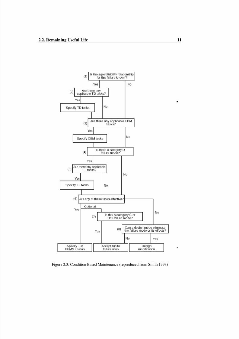
As Figure 2.3 illustrate, the rst step when starting CBM programme is to askif the failure of the component can be easily predicted in terms of aging. The nextstep is to plan an age based preventive maintenance routines (TD tasks). Generallythere would be some failure modes that can be individuated by TD tasks and others(CBM tasks) that might be detected only by inspections or by use of CMS. For agearbox, typical TD tasks might be a change of lubricant or seals while a CBM taskmight be polishing of the gears when a certain level of wear has been detected[12].
In some components, hidden (or latent) failures may be present and in those
cases some type of testing (Fault Finding Tasks) is carried out. Hidden failures arenormally occurring in passive items or machines that are normally not operatingand are only activated on demand, for example re detectors.
2.2 Remaining Useful Life
Instead of relying on average life-time statistics such as the MTTF to schedulemaintenance activities, condition based maintenance uses direct monitoring of theoperating conditions to determine the actual mean time to failure.However it cansometime be difcult to evaluate such information. This is, for example, the case
8/6/2019 Gearbox+ +Rossir24 0017
http://slidepdf.com/reader/full/gearbox-rossir24-0017 20/91
2.2. Remaining Useful Life 11
Figure 2.3: Condition Based Maintenance (reproduced from Smith 1993)

8/6/2019 Gearbox+ +Rossir24 0017
http://slidepdf.com/reader/full/gearbox-rossir24-0017 21/91
12 Chapter 2. Maintenance Theory
of a gearbox in wind turbines, where “the evaluation of the remaining useful life
(RUL) still remains a challenge”[13]. It is fundamental to know what it is theremaining time before the item fails in order to schedule a corrective action andtherefore avoiding production losses or major break downs.
The residual life or remnant life (RUL) is dened as a random variable T repre-senting the time left before the failure occurs given the machine condition, age andthe past operational condition. It is dened as the conditional random variable:
[T − t | T ≥ t, Z (t )]
where t is the current age and Z(t) is the past condition up to the current time.RUL is a random variable and therefore it would be of interest to fully understandits distribution[10]. it would might be useful also to calculate the statistical ex-pected value of the RUL also dened as RULE (Remaining Useful Life Estimate),i.e. E [T − t |T > t, Z (t)] .
2.3 Optimizing Condition Based Maintenance
There are three types ofdecisions which need to be made in the context ofcondition-based maintenance:
1. Selecting the component, the condition monitoring technique and the param-eters to be monitored
2. Determining the inspection frequency;
3. Establishing the warning limit (threshold level);
Selectingwhat to monitor depends on what type of equipment , instrumentationor training available and operating costs. It should be noted that a failure mayshow several types of symptoms which may be detectable at different stages of degradationof theunit. For example, theearliest warning signalof a bearing failureis in the form of changed vibration signature.
Inspection frequency optimization may play an important role in the case of off-line monitoring policy. Interval between inspections has to be determined, so thataction can be taken in time either to prevent functional failures or to minimizethe consequences of those which cannot be prevented[12]. The optimal inspectionfrequency is the one for which the minimum level of costs is obtained (Figure 2.4).

8/6/2019 Gearbox+ +Rossir24 0017
http://slidepdf.com/reader/full/gearbox-rossir24-0017 22/91
2.4. Condition Based Maintenance Models 13
Figure 2.4: Optimal scheduled MPM frequency
Figure 2.5 shows the deterioration process of a component with respect to time.By inspection or monitoring, the state of the component can be assessed and whenit reaches a certain level of deteriorationλ (i.e., threshold) preventive maintenancetasks should be triggered. Keeping in mind that the objective is to minimize costs,
establishing the optimal treashold can be quite challenging. If λ is chosen too low,a still functioning component might be replaced but on the other side an highervalue can increase the number of unexpected failures thus increasing correctivemaintenance which is typically more expensive.
Replacing the component before it fails makes it not possible to establish whatthe actual physical limit is, or until which degradation level the equipment can stillperform its functions. This can represent a problem when historical data for thecomponents are analyzed.
2.4 Condition Based Maintenance ModelsDekker in [14] suggests the following denition for a maintenance optimizationmodel:Those mathematical models whose aim it is to nd the optimum balancebetween the costs and benets of maintenance, while taking all kinds of constraintsinto account .In this denition benets are meant as savings in terms of avoidanceof production losses and costs that would occur due to failures (i.e.,repairs, manlabour, spare parts, etc.). When a maintenance model is developed is important totake into consideration the following factors [14]:
• Description of the technical system and its functions;

8/6/2019 Gearbox+ +Rossir24 0017
http://slidepdf.com/reader/full/gearbox-rossir24-0017 23/91
14 Chapter 2. Maintenance Theory
Figure 2.5: Deterioration process and threshold level that triggers preventive maintenance
• Model deterioration, determinerisks andcosts of failure and itsconsequencesas well as costs of maintenance;
• Description of the available information about the system (Maintenance rou-tines, Costs for maintenance, frequency of inspections);
• An objective function and optimization technique which helps in nding thebest balance.
The rst step consists in identify failure mechanisms, causes, and detectionand prevention methods. This involves the engineering aspects of the system understudy.The second phase is characterized by the selection of a deterioration model.The model can be built using the knowledge of failure mechanisms as well as theexisting data related to failures.
Failures can generally be divided into two categories random failures and thosearising as a consequence of deterioration (aging).Given the latter type of failures,deterioration process is represented by a sequence of stages of increasing wearwhich nally leads to equipment failure. Deterioration is often a continuous pro-cess in time and only for the purposes of easier modeling is it considered in discrete
steps[15]. Each deteriorating state can be dened both or else by the the level of physical deterioration (corrosion,wear) that the component presents. One of themost common mathematical technique to solve maintenance problems in whichthe states of component can be identied is the Markov chain.
There is usually a great amount of data to be analyzed and interpreted when acondition based maintenance is implemented. Data are not only acquired by CMSbut also by the SCADA (Section 4.3) and the CMMS. A CMMS is a ComputerizedMaintenance Management System and basically is a storage data relative to allmaintenance activities ( repairs, spare parts, costs for maintenance, personnel work
8/6/2019 Gearbox+ +Rossir24 0017
http://slidepdf.com/reader/full/gearbox-rossir24-0017 24/91
2.5. General Framework 15
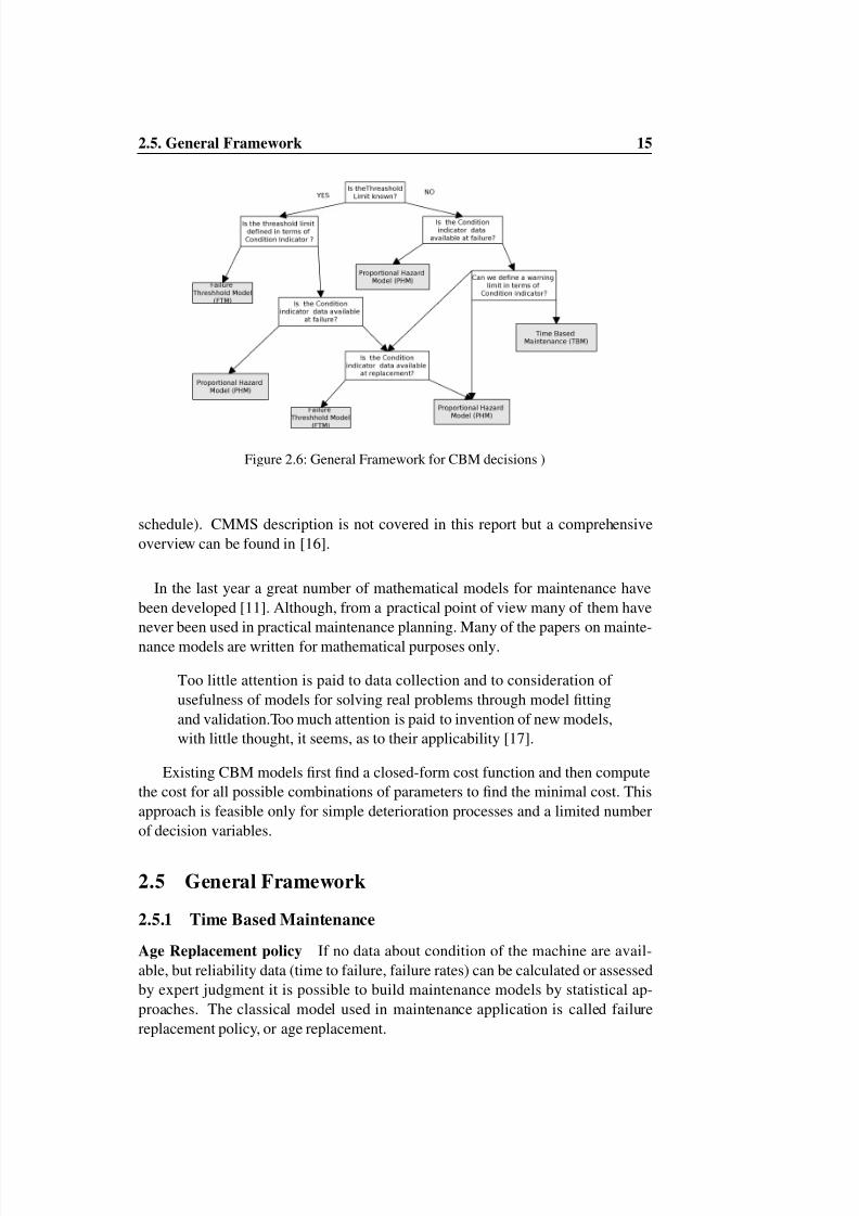
Figure 2.6: General Framework for CBM decisions )
schedule). CMMS description is not covered in this report but a comprehensiveoverview can be found in [16].
In the last year a great number of mathematical models for maintenance havebeen developed [11]. Although, from a practical point of view many of them havenever been used in practical maintenance planning. Many of the papers on mainte-nance models are written for mathematical purposes only.
Too little attention is paid to data collection and to consideration of usefulness of models for solving real problems through model ttingand validation.Too much attention is paid to invention of new models,with little thought, it seems, as to their applicability [17].
Existing CBM models rst nd a closed-form cost function and then computethe cost for all possible combinations of parameters to nd the minimal cost. Thisapproach is feasible only for simple deterioration processes and a limited numberof decision variables.
2.5 General Framework
2.5.1 Time Based Maintenance
Age Replacement policy If no data about condition of the machine are avail-able, but reliability data (time to failure, failure rates) can be calculated or assessedby expert judgment it is possible to build maintenance models by statistical ap-proaches. The classical model used in maintenance application is called failurereplacement policy, or age replacement.
8/6/2019 Gearbox+ +Rossir24 0017
http://slidepdf.com/reader/full/gearbox-rossir24-0017 25/91
16 Chapter 2. Maintenance Theory
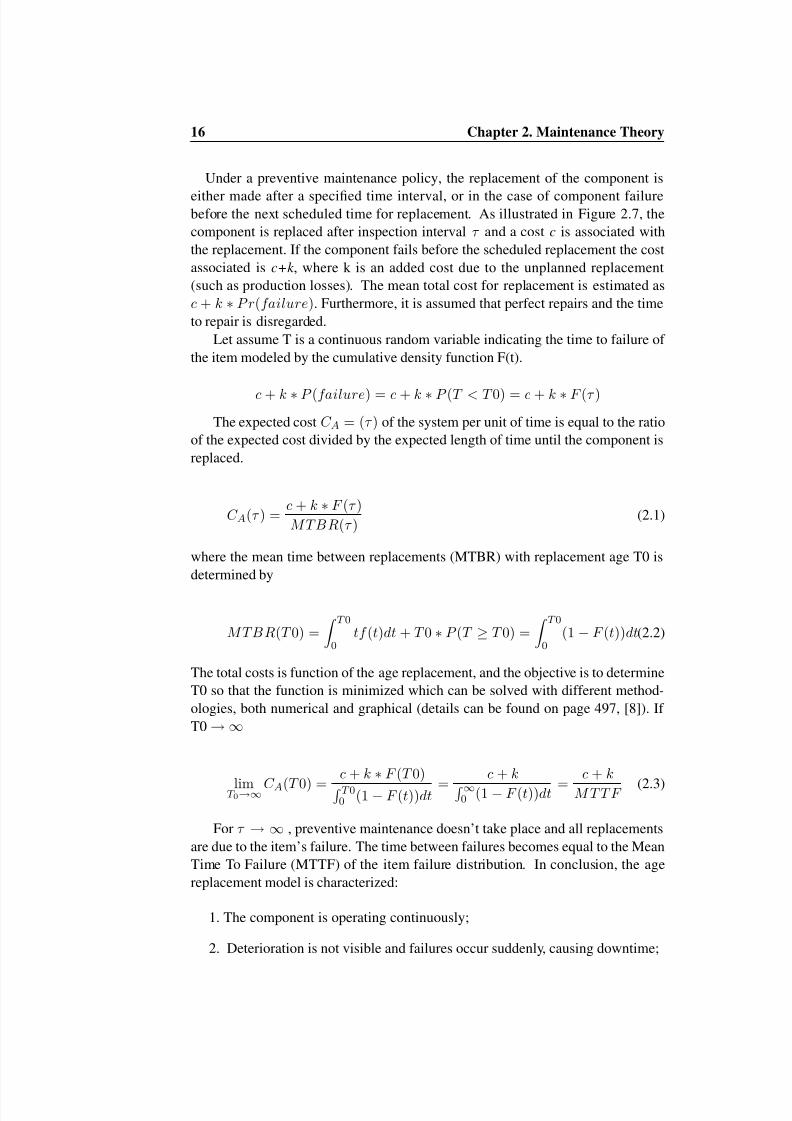
Under a preventive maintenance policy, the replacement of the component is
either made after a specied time interval, or in the case of component failurebefore the next scheduled time for replacement. As illustrated in Figure 2.7, thecomponent is replaced after inspection intervalτ and a costc is associated withthe replacement. If the component fails before the scheduled replacement the costassociated isc+k , where k is an added cost due to the unplanned replacement(such as production losses). The mean total cost for replacement is estimated asc + k ∗P r (failure ). Furthermore, it is assumed that perfect repairs and the timeto repair is disregarded.
Let assume T is a continuous random variable indicating the time to failure of the item modeled by the cumulative density function F(t).
c + k ∗P (failure ) = c + k ∗P (T < T 0) = c + k ∗F (τ )The expected costC A = ( τ ) of the system per unit of time is equal to the ratio
of the expected cost divided by the expected length of time until the component isreplaced.
C A(τ ) =c + k ∗F (τ )MTBR (τ )
(2.1)
where the mean time between replacements (MTBR) with replacement age T0 isdetermined by
MTBR (T 0) = T 0
0tf (t )dt + T 0∗P (T ≥ T 0) =
T 0
0(1 − F (t ))dt(2.2)
The total costs is function of the age replacement, and the objective is to determineT0 so that the function is minimized which can be solved with different method-ologies, both numerical and graphical (details can be found on page 497, [8]). If T0→ ∞
limT 0 →∞ C A(T 0) =c + k ∗F (T 0)
T 00 (1 − F (t ))dt =
c + k
∞0 (1 − F (t ))dt =
c + kM T T F (2.3)
Forτ → ∞ , preventive maintenance doesn’t take place and all replacementsare due to the item’s failure. The time between failures becomes equal to the MeanTime To Failure (MTTF) of the item failure distribution. In conclusion, the agereplacement model is characterized:
1. The component is operating continuously;
2. Deterioration is not visible and failures occur suddenly, causing downtime;

8/6/2019 Gearbox+ +Rossir24 0017
http://slidepdf.com/reader/full/gearbox-rossir24-0017 26/91
2.5. General Framework 17
Figure 2.7: Age Replacement Policy (Adapted from [8])
3. The component is replaced upon failure by an identical one with costs c(including costs for downtime) and preventively with a costs c+k (wheneverit takes place);
4. The failure rate or the probability density functionof the component is known
5. The Objective function is the long-term total cost function
2.5.2 Block Replacement
The block replacement policy is similar to the ARP, but we do not reset the main-tenance clock if a failure occurs in a maintenance period or in other words westill replace the component at scheduled time before the failure occured. The BRPseems to be "wasting" some valuable component life time, since the componentis replaced at an age lower than if a failure occurs in a maintenance period [18].However, this could be defended due to administrative savings, or reduction of set-up cost if many components are maintained simultaneously. In this situation, themaintenance cycle length is xedτ , and the average number of failures per unittime is given by the expected number of failures in (0,t):
λ BR =Expected no. of failures
τ =
W (τ )τ
Where W(t) is the renewal function discussed later on. If τ is small comparedto the MTTF of the component, it is very unlikely to have more than one failurewithin one maintenance cycle. In this case W(t) can be approximated with F(t).
2.5.3 Markov State Modelling
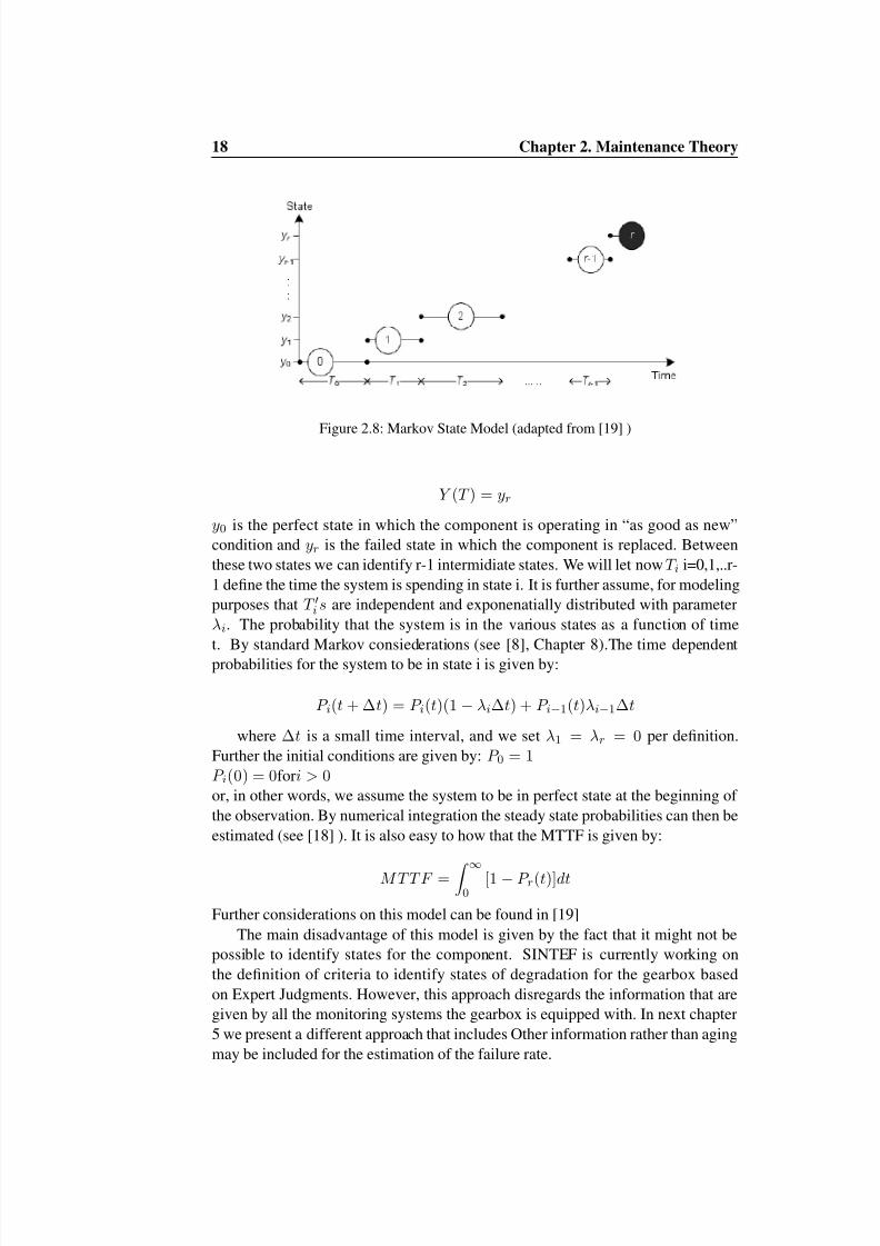
Markov Processes are often employed for modelling maintenance planning. Thecharateristic of such models is that the system in is is identied with a nite num-ber of states We here present a model developed at SINTEF [19] for maintenancedecision on hydropower turbines. T is dened as the time to failure (see Figure2.8). The system state Y(t) at time t:
Y (0) = y0
8/6/2019 Gearbox+ +Rossir24 0017
http://slidepdf.com/reader/full/gearbox-rossir24-0017 27/91
18 Chapter 2. Maintenance Theory
Figure 2.8: Markov State Model (adapted from [19] )
Y (T ) = yr
y0 is the perfect state in which the component is operating in “as good as new”condition andyr is the failed state in which the component is replaced. Betweenthese two states we can identify r-1 intermidiate states. We will let nowT i i=0,1,..r-1 dene the time the system is spending in state i. It is further assume, for modelingpurposes thatT i s are independent and exponenatially distributed with parameterλ i . The probability that the system is in the various states as a function of timet. By standard Markov consiederations (see [8], Chapter 8).The time dependentprobabilities for the system to be in state i is given by:
P i(t + ∆ t ) = P i (t )(1 − λ i∆ t ) + P i− 1(t )λ i− 1∆ t
where∆ t is a small time interval, and we setλ 1 = λ r = 0 per denition.Further the initial conditions are given by:P 0 = 1P i (0) = 0 fori > 0or, in other words, we assume the system to be in perfect state at the beginning of the observation. By numerical integration the steady state probabilities can then beestimated (see [18] ). It is also easy to how that the MTTF is given by:
M T T F = ∞
0[1 − P r (t )]dt
Further considerations on this model can be found in [19]The main disadvantage of this model is given by the fact that it might not be
possible to identify states for the component. SINTEF is currently working onthe denition of criteria to identify states of degradation for the gearbox basedon Expert Judgments. However, this approach disregards the information that aregiven by all the monitoring systems the gearbox is equipped with. In next chapter5 we present a different approach that includes Other information rather than agingmay be included for the estimation of the failure rate.
8/6/2019 Gearbox+ +Rossir24 0017
http://slidepdf.com/reader/full/gearbox-rossir24-0017 28/91
2.6. Failure Modes and Criticality Analysis 19
2.6 Failure Modes and Criticality Analysis
TheFailure Modes,Effects andC riticalityAnalysis (FMECA) is a systematic in-ductive methodology used to dene, identify, prioritize and eliminate known and/orpotential failures, problems, errors, and so on from the system, design and process.In many industries it is used during the whole life cycle of the product/system,with different goals and purposes throughout the different stages of the equipmentlife. It is usually performed in the conceptual and initial design phases to assurethat all conceivable failure modes and their possible effects on the system as earlyas possible.During the development phase it can be a powerful tool for designingreliability into the system. It is also used as documentary purposes and provides abasis for maintenance planning.
Originally it was called FMEA (Failure Modes and Effects Analysis) and rstdeveloped by the United Sates Military in 1949 with the goal of reducing acci-dents and near missed in aerospace industry.The most important contribution of FMECA with respect to FMEA that by focusing on Criticality one can identify theso calledsingle point failure mode .However in many texts and other sources,theterms FMEA and FMECA are used to explain the same methodology and usuallyboth include the criticality analysis. The Military Standard MIL-STD-1629A isone of the most spread standard on FMECA.
FMECA is an indispensable tool when Reliability Centred Maintenance (RCM)approach is adopted.It is used to identify what are the most critical components,their failure modes and to rank them according with the consequences they mighthave on the system.
2.6.1 FMECA Procedure
A general FMECA analysis regardless on type andapplication is performedthroughseveral steps. Figure 2.9 describes the different stages together with the feedbacksthat each step is feeding to the others. The different steps can be summarized in:
1. System Denition : The system´s boundaries have to be dened, its mainfunctions identied. Operational and environmental conditions have to beconsidered;
2. Data Collection : Collect all available data on the system, such as drawings,specications, component lists. Information about previous and similar de-signs from various sources can be useful;
3. System’s analysis : Analyze and describe the system using functional blockdiagrams or other relevant methodologies;

8/6/2019 Gearbox+ +Rossir24 0017
http://slidepdf.com/reader/full/gearbox-rossir24-0017 29/91
20 Chapter 2. Maintenance Theory
4. Preparation of FMECA worksheet : Examine thesystemforpossible failures,
their causes and effects. The severity of these failures and their probabilityto occur have to be assessed. The results are recorded on the FMECA work-sheet;
5. Criticality Analysis : Rank the possible failures according to the risk theymay represent.This is done using qualitative or quantitative methods;
6. Review : Team of experts with different backgrounds but relevant for thespecic system evaluates the work sheet through discussions.;
7. Introduction of corrective actions into the system ;
8. Documentation of results .
Figure 2.9: FMECA process (Adapted from Fmea Military Handbook 470A)
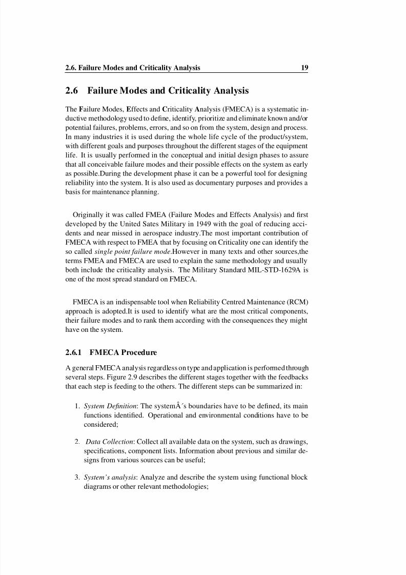
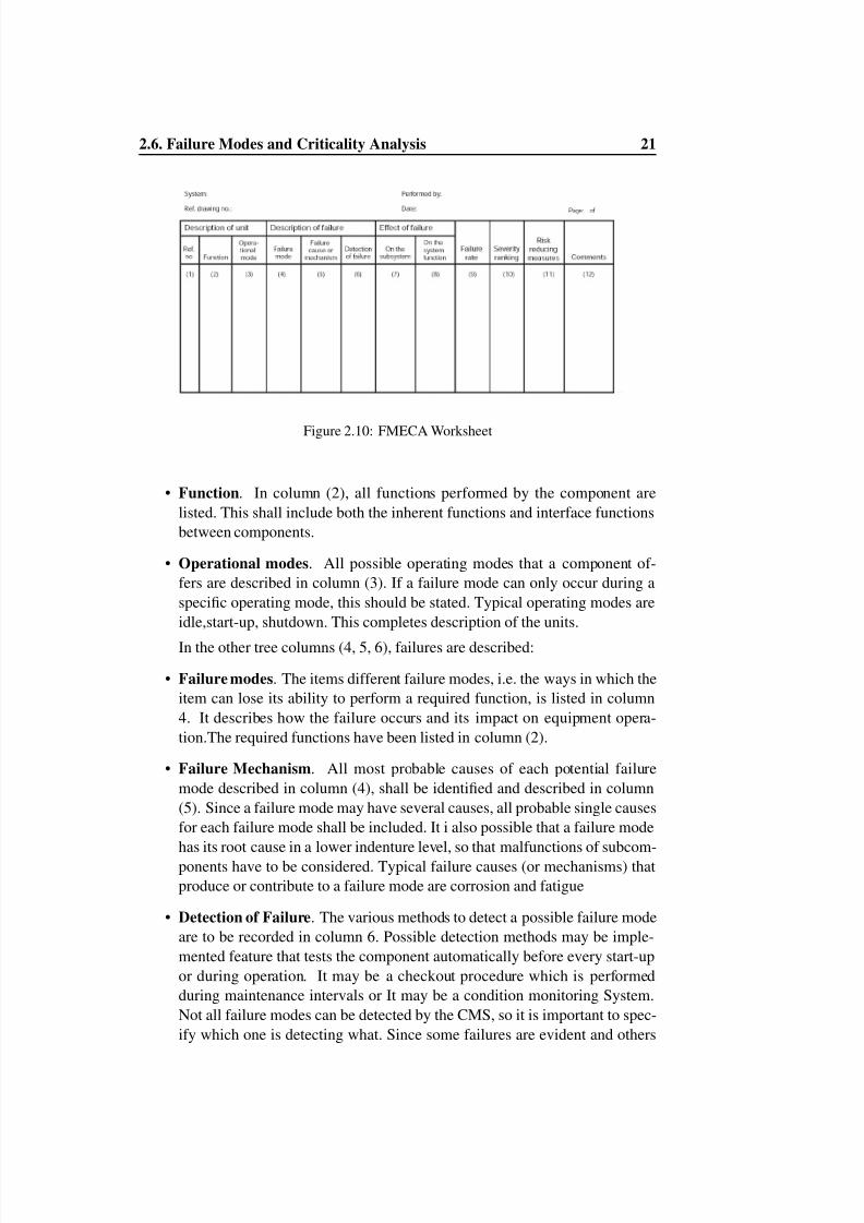
2.6.2 FMECA Worksheet preparationAfter the system has been dened using by block diagrams, the next step fol-lows: The preparation of the FMEA-worksheet. A typical worksheet is shownin Figure 2.10. On it, all aspects and functional units that could cause failures areregistered[20][21].
In the rst three columns, description of components are described:
• Id. component . Every one of these items gets an identication number,which is written into column (1). This number may be a serial number oranother identifying code (tag number) and serves for traceability purposes.
8/6/2019 Gearbox+ +Rossir24 0017
http://slidepdf.com/reader/full/gearbox-rossir24-0017 30/91
2.6. Failure Modes and Criticality Analysis 21
Figure 2.10: FMECA Worksheet
• Function . In column (2), all functions performed by the component arelisted. This shall include both the inherent functions and interface functionsbetween components.
• Operational modes . All possible operating modes that a component of-fers are described in column (3). If a failure mode can only occur during aspecic operating mode, this should be stated. Typical operating modes areidle,start-up, shutdown. This completes description of the units.
In the other tree columns (4, 5, 6), failures are described:• Failure modes . The items different failure modes, i.e. the ways in which the
item can lose its ability to perform a required function, is listed in column4. It describes how the failure occurs and its impact on equipment opera-tion.The required functions have been listed in column (2).
• Failure Mechanism . All most probable causes of each potential failuremode described in column (4), shall be identied and described in column(5). Since a failure mode may have several causes, all probable single causesfor each failure mode shall be included. It i also possible that a failure modehas its root cause in a lower indenture level, so that malfunctions of subcom-ponents have to be considered. Typical failure causes (or mechanisms) thatproduce or contribute to a failure mode are corrosion and fatigue
• Detection of Failure . The various methods to detect a possible failure modeare to be recorded in column 6. Possible detection methods may be imple-mented feature that tests the component automatically before every start-upor during operation. It may be a checkout procedure which is performedduring maintenance intervals or It may be a condition monitoring System.Not all failure modes can be detected by the CMS, so it is important to spec-ify which one is detecting what. Since some failures are evident and others
8/6/2019 Gearbox+ +Rossir24 0017
http://slidepdf.com/reader/full/gearbox-rossir24-0017 31/91
22 Chapter 2. Maintenance Theory
stay hidden, it should be distinguished between these two types of failures
in this column. A pump´s failure mode ”fail to start´´, for example, ishidden during stand by). It may be favorable to mention how likely detec-tion is. Ranks on a scale (typically from 1 to 5) that covers from certainty todetecting the failure to inability of doing so.
• Effects . The failure effects are described in columns (7) and (8). A failureeffect is the consequence of one or many failure modes in terms of the oper-ation, function or state of a system. Failures that affect only the componentunder consideration or its subcomponents are calledlocal failure effects andare recorded in column (7). All consequences of all possible failure on theoutput of the component have to be described. This serves the purpose of
evaluating compensating provisions and recommending corrective actions.Global failure effects are effects that occur on the system level. They mayresult in total or partly malfunctions, reduction of output, change of oper-ational mode or other deciencies. To improve the analysis, a distinctionbetween categories of effects should be considered. These categories can besafety effects, environmental, production availability, or economic effects.
• Failure Rates . In column (9), the rates of occurrence (i.e, failure rates) of identied failure modes are recorded. A possible classication as suggestedin IEC standard 60812 could be:
1 Very unlikely Once every 1000 years or more seldom2 Remote Once every 100 years3 Occasional Once every 10 years4 Probable Once every year5 Frequent Once every month or more often
• Severity Rankinking . In Column (10) it is assessed how severe the con-sequences of a failure mode are estimated on the system level.A possibleclassication for Severity may be:
I: Insignicant: Only minor damage to system and no injury to personnelcaused by failure mode;II: Marginal: A failure which may cause minor injury, minor property dam-
age, or minor system damage which will result in delay or loss of avail-ability respectively in system degradation;
III: Critical: A failure which may cause severe damage, or major systemdamage;
IV: Catastrophic: A failure which may result in loss of property or completedamage of the system;

8/6/2019 Gearbox+ +Rossir24 0017
http://slidepdf.com/reader/full/gearbox-rossir24-0017 32/91
2.6. Failure Modes and Criticality Analysis 23
Other categories are of course feasible and may be developed in consider-
ation of several factors such as effects on the environment resulting fromfailure, government regulations or requirements implied by warranties.
• Countermeasures . Measures that have to be taken to reduce the risk areidentied, evaluated and collected in column (11). They include precautionsthat mitigate the effects of the failure or its rate of occurrence and increase tprobability of its detection.
• Column (12) can be used for comments and additional information that hasnot been included in the previous columns.
Criticality AnalysisCriticality Analysis is a methodology used to determine how critical each detectedfailure mode is. By using this tool, it can be discovered which items need revisionin order to reduce the impact of the corresponding failure modes on the system.Threats can be mitigated through limiting the severity of a failure effect or its rateof occurrence.
Risk Priority Number A common quantitative method to assess criticality is theRisk Priority Number (RPN). The risk is evaluated as:
RP N = S ∗O ∗D
S denotes a subjective measure of how severe the effect of a failure is on the systemlevel (Severity Ranking), O is the probability of occurrence and can be expressed interms of failure rates or in the form of a ranking number. D denotes the probabilityof nding a failure before the system is affected (Detection).
Any ranking scales can be utilized, however typically an higher number indi-cates a worse chance of detecting the failure. Deciding which failure mode is tobe mitigated is made upon the magnitude of the RPN. Although, this decision ismainly inuenced by the expected severity of a failure mode, so that if two failuremodes have the same RPN, the one with the higher severity is to be addressed rst.The following table shows a possible ranking scale that may be adopted[20]:
Likelihood of detection Ranking (D)
Almost certain 1High 2
Moderate 3Low 4
Remote 5Absolutely uncertain 6
8/6/2019 Gearbox+ +Rossir24 0017
http://slidepdf.com/reader/full/gearbox-rossir24-0017 33/91
24 Chapter 2. Maintenance Theory
Team Review
All FMECA are team based but there should always be a single person responsiblefor the process. It should be initiated by the design engineer for the hardwareapproach, and the systems engineer for the functional approach. After the initialanalysis is completed, the team should review the process[22].
The purpose of the team is to bring together different perspectives and experi-ences to the analysis. FMECA team are are formed on temporary basis (i.e, untilthat specic FMECA is complete) and their composition depends upon the typeof project.The best size for the team is usually four to six people. Manufacturing,engineering, maintenance representatives should be represented in the team[23]. It
can be helpful to have people with different level of familiarity with the productor process. The most familiar ones will have valuable insights but may overlooksome of the most obvious potential problems while the less familiar ones will bringunbiased and objective ideas into the FMEA process. People directly involved withthe development or the process or product might be over sensitive when it comesto criticize the process and may become defensive. As previously said there shouldalways be a team leader, although he shouldn’t have any nal word on team deci-sions and his main role should only consist basically in setting up and facilitatingmeetings,ensuring team necessary resources available and team progression towardcompletion.
Corrective Actions
After all failure modes have been identied and ranked, it can be decided whichdesign deciencies shall be addressed rst and which can be postponed. Coun-termeasures may include changes in the design or the implementation of specicmaintenance tasks.
Documenting the Results
At the end of the FMECA a report has to be drawn up. This report may be per-formedin various scopes, but there areessential features it shouldcontain. It should
include a detailed record of the analysis as well as the block or functional diagramsthat dene the system´s structure. Furthermore worksheets, summaries of results,data sources and descriptions of the techniques used during the analysis need to beincluded. Recommendations for the elimination of further failure risk should beincluded, as well as a list of items which are critical to future reliability. This listshows:
• Item identication
• Description of the design features which minimize the occurrence of failurefor the listed item

8/6/2019 Gearbox+ +Rossir24 0017
http://slidepdf.com/reader/full/gearbox-rossir24-0017 34/91
2.6. Failure Modes and Criticality Analysis 25
• Description of tests that verify design features and tests that would detect the
failure mode occurrence• Description of planned inspections to ensure hardware is being built to de-
sign requirementsand inspections planned duringdown-time or maintenancethat could detect a failure mode or conditions that could cause a failure mode
• A statement relating to the history of this particular or similar design
• Description of the methods by which the occurrence of a failure mode canbe detected by the operator and whether a failure of a redundant operatingmode can be identied
The report shall also provide a list of all single failure points. These single failurepoints are failure of items which cannot be compensated by redundancy or alterna-tive operational procedures. Their criticality classication should be mentioned.

8/6/2019 Gearbox+ +Rossir24 0017
http://slidepdf.com/reader/full/gearbox-rossir24-0017 35/91
8/6/2019 Gearbox+ +Rossir24 0017
http://slidepdf.com/reader/full/gearbox-rossir24-0017 36/91
Chapter 3
System Description: The
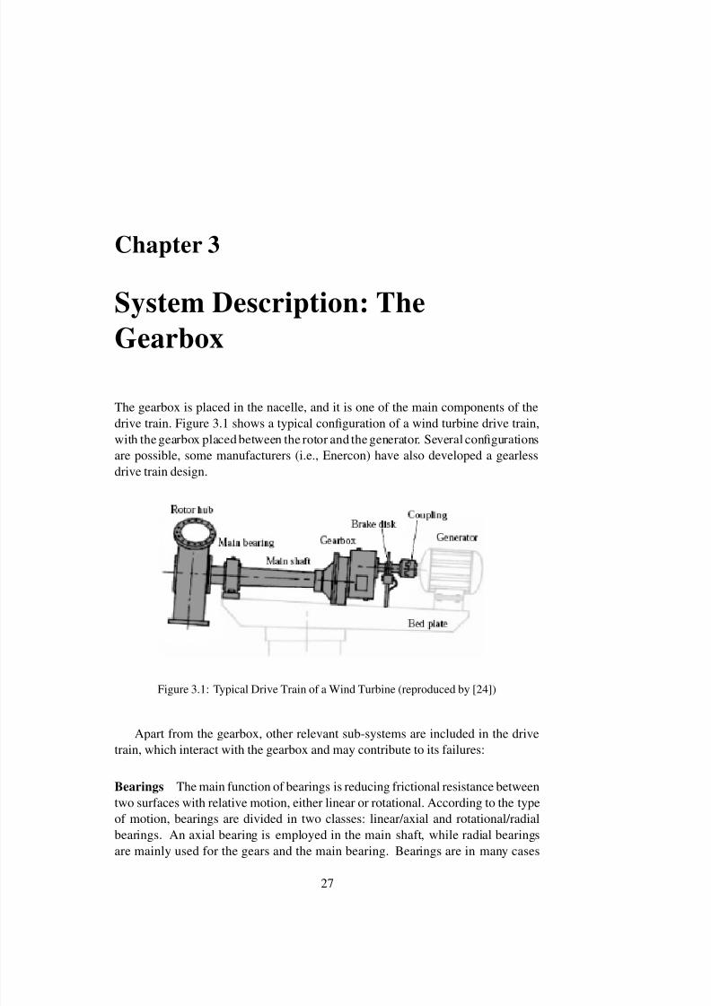
GearboxThe gearbox is placed in the nacelle, and it is one of the main components of thedrive train. Figure 3.1 shows a typical conguration of a wind turbine drive train,with thegearbox placedbetween the rotor and thegenerator. Several congurationsare possible, some manufacturers (i.e., Enercon) have also developed a gearlessdrive train design.
Figure 3.1: Typical Drive Train of a Wind Turbine (reproduced by [24])
Apart from the gearbox, other relevant sub-systems are included in the drivetrain, which interact with the gearbox and may contribute to its failures:
Bearings The main function of bearings is reducing frictional resistance betweentwo surfaces with relative motion, either linear or rotational. According to the typeof motion, bearings are divided in two classes: linear/axial and rotational/radialbearings. An axial bearing is employed in the main shaft, while radial bearingsare mainly used for the gears and the main bearing. Bearings are in many cases
27

8/6/2019 Gearbox+ +Rossir24 0017
http://slidepdf.com/reader/full/gearbox-rossir24-0017 37/91
28 Chapter 3. System Description: The Gearbox
responsible for gearbox failures [25][26][4].
Shafts Cylindrical elements designed to rotate with the function of transmittingtorque. In a drive train there are several shafts and they can be distinguished be-tween low speed (on the rotor side) and high speed shafts (on the generator side).Intermediate shafts are typically placed in the gearbox housing and their aim is tocarry the gears.
Couplings Couplings are elements used to connect two shafts together for thepurpose of transmitting torque between them. A typical use of couplings in windturbines is the connection between the generator and the high speed shaft of thegearbox. In some design, a safety clutch is integrated into the coupling to protectthe gearbox by preventing the transfer of torque transient in the case of a possiblegenerator’s short circuit.
Mechanical Brakes A mechanical friction brake and its hydraulic system is usedto halt the turbine blades during maintenance and overhaul, or in emergency cases.Use of brakes can also introduce dynamic loads on the gearbox.
As long as the braking torque and braking power (thermal loading) can beabsorbed, the rotor brake can be used as a second independent braking system inaddition to aerodynamic rotor braking. With increasing turbine size, it becomes
more and more difcult to meet this requirement since the brake would take absurddimensions. For this reason, the task of the rotor brake in large turbines is alwaysrestricted to the function of pure parking brake.
Another important issue to be considered by manufacturers is where in the drivetrain the rotor brake should installed. The rotor brake can be either put on the lowspeed side or on the high speed side of the gearbox (section 3.1). The two possiblealternatives are either onlow-speed or on thehigh-speed side of the gearbox. Inmost turbines, efforts to keep the brake disk diameter as small as possible lead tothe rotor brake being installed on the high-speed shaft, i. e. between gearbox andgenerator. In fact due to mechanical energy balance, a lower torque magnitudecorresponds to an higher rotational speed.
Mounting the brake on the high-speed shaft has at least two disadvantages: thebraking function fails if the low-speed shaft or the gearbox break down and thegearbox is exposed to increased wear.During standstills, gears are subjected to in-creased because of small oscillating movements which areunavoidable in a stoppedwind turbine due to air turbulence. In some turbines, it is attempted to solve thisproblem by no longer locking the rotor during standstill but by letting it spin at lowspeed.
8/6/2019 Gearbox+ +Rossir24 0017
http://slidepdf.com/reader/full/gearbox-rossir24-0017 38/91
3.1. Gears 29
To avoid these disadvantages, the rotor brake was installed on the low-speed
rotor shaft in small wind turbines.However, installing the rotor brake on the slowside is much more problematic in large wind turbines and this has led to the rotorbrake being arranged on the high-speed side behind the gearbox in almost all newsystems.
3.1 Gears
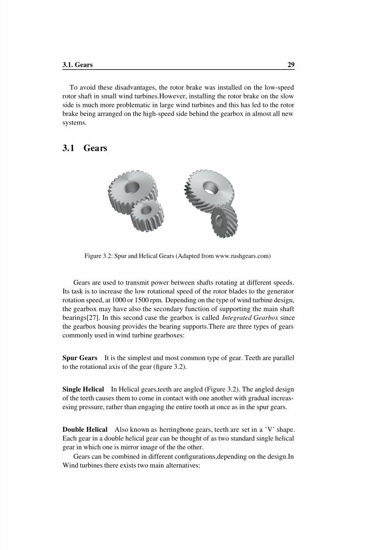
Figure 3.2: Spur and Helical Gears (Adapted from www.rushgears.com)
Gears are used to transmit power between shafts rotating at different speeds.Its task is to increase the low rotational speed of the rotor blades to the generatorrotation speed, at 1000 or 1500 rpm. Depending on the type of wind turbine design,the gearbox may have also the secondary function of supporting the main shaftbearings[27]. In this second case the gearbox is calledIntegrated Gearbox sincethe gearbox housing provides the bearing supports.There are three types of gearscommonly used in wind turbine gearboxes:
Spur Gears It is the simplest and most common type of gear. Teeth are parallelto the rotational axis of the gear (gure 3.2).
Single Helical In Helical gears,teeth are angled (Figure 3.2). The angled designof the teeth causes them to come in contact with one another with gradual increas-esing pressure, rather than engaging the entire tooth at once as in the spur gears.
Double Helical Also known as herringbone gears, teeth are set in a ’V’ shape.Each gear in a double helical gear can be thought of as two standard single helicalgear in which one is mirror image of the the other.
Gears can be combined in different congurations,depending on the design.InWind turbines there exists two main alternatives:

8/6/2019 Gearbox+ +Rossir24 0017
http://slidepdf.com/reader/full/gearbox-rossir24-0017 39/91
30 Chapter 3. System Description: The Gearbox
Parallel Stage In this conguration, gears are carried on two parallel shafts that
are supported by bearings. The two gears are of different size, and the one on thelow-speed shaft is the largest. The relation between their rotational speeds ratiois inversely proportional to the number of teeth. It exists a physical limit of themaximum obtainable ratio, and this is the reason why multiple stages have to beused.
Planetary Stage The other possible solution utilized in wind turbines gearboxesis the planetary stage. The main components of this typology of gear are illustratedin Figure 3.3:
• An interior toothed gear wheel (ring gear );
• Two or three smaller toothed gear wheels ( planet gear );
• A common carrier arm (planet carrier );
• A centrally placed toothed gear wheel (the sun gear );
Figure 3.3: Planetary Stage
The ring gear is stationary while the planet carrier is mounted on the rotor shaftwhich rotates with the same rotational speed as the rotor blades. The planet carriertransmits the driving torque to the planet gears that move around inside the innercircumference of the ring wheel. The rotational speed of the centrally placed sungear wheel is increased. The speed-up ratio for this conguration can be expressesby the following [27]:
n HSS
n LSS = 1 +
D ring
D sun(3.1)

8/6/2019 Gearbox+ +Rossir24 0017
http://slidepdf.com/reader/full/gearbox-rossir24-0017 40/91
3.1. Gears 31
wheren HS S and n LSS are respectively the rotational speed of the sun and the
planet carrier,D ring is the diameter (or number of teeth) of the ring wheel andD sun Diameter (or number of teeth) of the sun.Typically it is obtained a gear ratioof about 1:5 [26].
As power and rotor diameter increase the torque and gear ratio also increase andoften one single gear stage is not sufcient. Multiple stages of gears are thereforerequired in order to obtain the desired ratio.Large wind turbine (typically largerthan 500 KW) have an integrated gearbox with a planet gear and two normal stages.
Figure 3.4: Planetary Stage and two Parallel Stages (single helical gears)
Advantages of using a Planetary Gearbox:
• Increase of the efciency and provides extremely low speeds,
• Delivers high reduction ratios and transmit a higher torque,
• Compact and lightweight, little installation space,
• High reliability due to proper distribution of stress among different bearingcomponents,
Gearbox dimensioning Dimensioning in a correct manner the gearbox is a fun-damental task in order to reduce incipient failures and increasing inherent relia-bility. Typically the dimensioning is carried out by the manufacturers. The mostimportant parameter is thetorque to be transmitted. The rotor torque is not a con-stant value but is subject to large variations, depending on the technical design con-cept of the wind turbine. According to DIN 3990 (German National Standards),
8/6/2019 Gearbox+ +Rossir24 0017
http://slidepdf.com/reader/full/gearbox-rossir24-0017 41/91
32 Chapter 3. System Description: The Gearbox
the quotient of the equivalent torque Teq and the rated torque is calledapplication
factor K A and it is dened as:
K A =T eq
T N
whereT N is the rated torque to be transmitted, obtained very simply by divid-ing the rated mechanical rotor power by the rotor speed. However The rotor torqueis, of course, not a constant value but is subject to more or less large variations,therefore we talk about torque spectrum,expressed as magnitude and frequency oc-curring over the entire operating life of a turbine. Based on this load spectrum,the equivalent torqueT eq can be estimated as dened in the DIN 3990 standard.If no load spectrum is available, the application factor KA, and with it the equiv-
alent torque,must be determined empirically from comparisons with similar casesof application.
There are at least two more factors in gearbox technology which are in use forcharacterizing the external load situation for the transmission. In English-speakingcountries, the so-calledservice factor is used and it is dened in the AGMAstandards. In view of the numerous denitions, the designer of the wind turbinesystem must have a clear agreement with the gearbox manufacturer regarding thedimensioning factors to be applied [28].
WindTurbinegearboxes are typicallydesigned to havea breakingstrength whichis at least three times the rated torque. Only the ”generator short circuit load´´case can cause a higher torque peak in the drive train. In order to protect the gear-box and the rotor shaft from this, overload clutches are built into the high-speedshaft in most cases.
3.2 Lubrication and Cooling
The function of the lubrication system is to maintain an oil lm on gear teeth andthe rolling elements of bearings, in order to minimize surface pitting and wear(section 3.5). Different types of lubricants are available, and the selection of the
most suitable is dependent on gearbox design and its operational condition.The quality of the lubrication has been found to be a decisive factor for the
service life of the gearbox. Oil temperatures which are too high cause just as muchdamage as does contamination in the oil. Oil coolers and lters are indispensablefor large gearboxes and so is the careful observance of oil change intervals [29].Two alternative methods of lubrication are available:
- Splash lubrication ;
- Pressure fed ;
8/6/2019 Gearbox+ +Rossir24 0017
http://slidepdf.com/reader/full/gearbox-rossir24-0017 42/91
3.3. Operation and Maintenance Activities 33
In the Splash lubrication, the low-speed gear dips into an oil bath and the oil thrown
up against the inside of the casing is channeled down to the bearings [28]. In thePressure fed, oil is circulated by a pump, ltered and delivered under pressureto the gears and bearings. The advantage of splash lubrication is its simplicityand reliability, but pressure fed lubrication is usually preferred for the followingreasons:
• Oil can be directed where it is required by jets,
• Wear particles can be removed by ltration,
• Oil circulation system enables heat to be removed much more effectivelyfrom the gearbox by passing the oil through a cooler.
With a pressure fed system, it is normal practice to t temperature and pressureswitches downstream of the lter to trip the machine for excessive temperature orinsufcient pressure. Guidance on the selection of lubricant, which has to takeinto account the ambient temperatures, is given in the AGMA standards. Heatersmay be needed to enable oil to be circulated when the turbine starts up at lowtemperatures[28]. It is important that oil is at the correct temperature when thegearbox is working, to assure an effective viscosity and lm thickness.The ISOstandard 81400 concerning design of gearboxes for wind turbines, suggests thatturbine greater than 500 kW should be equipped with a pressure fed lubricationsystem.
Start up, operating and maintenance procedures should be established by thegearbox manufacturer and the purchaser before the gearbox is placed in service(IEC 61400-1). Oil change can be scheduled both on xed or condition based timeintervals:
• Fixed Time . When monitoring is too infrequent or not available or viabilityto the site is limited due to seasonal or location constraints. Changes intervalmust be based on past experience and a adjusted for the site environmentalconditions.
• Condition Based . When online or frequent monitoring of the oil is availableand considered reliable.
3.3 Operation and Maintenance Activities
According with the ISO standard 81400 ( Wind turbines: Design and specicationof gearboxes) operation and maintenance for a specic machine should be denedat the early stage (in the pre-commissioning phase) and should involve gearboxmanufacturer lubricant manufacturer and purchaser (typically an utility company).Start-up procedures may include the following checks:

8/6/2019 Gearbox+ +Rossir24 0017
http://slidepdf.com/reader/full/gearbox-rossir24-0017 43/91
34 Chapter 3. System Description: The Gearbox
• Oil level and type;
• Torque on gearbox bolts;
• Operation of automatic shutdown and alarms;
• Coupling installation and alignment;
• Heater, cooler, and fan start up;
• Minimize the shaft misalignment
In the case of wind farms not equipped with CMS, maintenance action haveto be taken about two times a year, as could be deduced from the state-of-the-artfailure frequency[13]. Usually a repair action is taken by a crew of two persons thatdrive to the failed wind turbine with a service van. They enter the wind turbine andtry to determine the cause of the failure and either start their repair action or cometo the conclusion that extra equipment and/or spare parts are needed for the repairaction. The extra equipment can either be or a crane for heavier lifting operations.”The repair time can be anything between an hour for a simple inspect and reset action to some weeks, when an exchange of a major component turns out to benecessary [30]”.
3.4 Costs for Operation and Maintenance
Even if it is true that wind turbines do not consume any fuel but utilize the freeunlimited source of the wind, it is equally true they can not work completely with-out operating costs. Maintenance and repairs, insurance and several other expensesrepresent themajor components of the operating costs.Thegreatest part of theoper-ating costs are indeed represented by the maintenance. After the initial investmentfor installation (around 70 % of total life cycle costs Most of maintenance costs area xed amount per year for regular service of the turbines.
An alternative method to calculate costs is to use a xed amount per kWh pro-duced. The reasoning behind this method is that wear on the turbine increases
with increasing production. Costs vary dramatically depending if the wind farmis onshore or offshore. In the latter case maintenance operations includes costs of viability (vessels, cranes and other equipment) and accessibility to the site is highlydependent on weather conditions and therefore downtime losses may become se-vere. Maintenance costs generally falls into the following categories:
Unscheduled maintenance Unscheduled or corrective maintenance is the mostcostly type of maintenance and it is usually a major aim for management to reduceit.The objective is to restore the equipment after wind turbine failures.A certainamount of unscheduled maintenance must be included within the life cycle of a

8/6/2019 Gearbox+ +Rossir24 0017
http://slidepdf.com/reader/full/gearbox-rossir24-0017 44/91
3.4. Costs for Operation and Maintenance 35
wind turbine. Wind turbines are formed by many complex sub-systems and these
components are rarely redundant, which means that even a minor failure very oftenwill lead to complete shutdown.
Unscheduled costs can grouped into into direct and indirect costs. The directcosts are associated with the labor and equipment costs required to repair the windturbine. The indirect costs result from production loss during turbine downtime.However, the actual cost may vary due to the wait time during high-wind con-ditions. The availability of some of the necessary equipment (cranes, vessels) islimited in many of the remote locations where wind farms are being installed andrepresents a major portion of the repair cost.
Planned maintenance The objective is to replace components that have limitedlife time, usually much shorter than the projected life of the turbine. These tasksinclude replacement of consumables such as brake pads and seals, inspections of the equipment’s condition (i.e., Scheduled Overhauls), oil and lter changes, cali-bration of sensors. The frequency for these tasks are identied in the maintenancemanuals provided by manufacturers and components suppliers. Costs associatedwith planned maintenance are easily evaluated but can vary in relation with locallabor cost and the location and accessibility of the site [3].
A description about different types of maintenance policies is given in section
2. Further distinction of O&M costs can be made by distinguishing between xedand variable costs [27], where variable costs are mainly represented by unsched-uled maintenance. ECN (Energy Center of Netherlands) has carried on a researchprogramme [31] with the scope of developing an operation and costs estimatorwith focus on offshore wind farms. Given that the biggest uncertainties in termsof costs are represented by unexpected faults, the model developed by ECN takesinto account reliability parameters together with material costs, personell , devicesneeded and logistics, for each subcomponents.
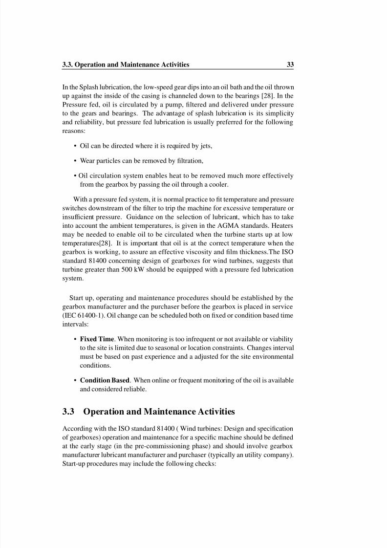
Figure 3.5 shows the costs for corrective maintenance over the lifetime. In theearly phases the costs are low mainly because new turbines come with a two yearservice contract, which includes preventive, maintenance, corrective maintenance,and warranties.These contracts can sometimes be extended to ve years. From thefth year on, the costs for corrective maintenance become somewhat unpredictable.Thus it becomes important to estimate the costs in the long term and it can also beobserved how maintenance costs are lower for bigger turbines.
Almost all manufacturers offer maintenance and service for the wind turbinesthey supply. These contracts can contain various services, from routine mainte-nance to ”all-inclusive”. Operating materials and large spare parts are usually ad-ditionally charged, unless they are included in the warranty that normally covers aperiod of ve years after commissioning[33].
8/6/2019 Gearbox+ +Rossir24 0017
http://slidepdf.com/reader/full/gearbox-rossir24-0017 45/91
36 Chapter 3. System Description: The Gearbox
Figure 3.5: Corrective maintenance costs during turbine’s life span (ISET) [32].
Other Operating Costs The operator of a wind turbine will normally try to coverthe nancial risks associated with operating the turbine as far by insurances. cov-ered by the following insurances:Liability insurance (risks against damage claimsby third parties), Insurance against machine breakage,Loss-of-prot insurancewhich covers the loss of revenue which was caused by a technical defect or aninterruption of operation not attributable to the operator.
Besides costs of maintenance and repair and the required insurances, there areother operating costs which must be considered for a complete operating cost eval-uation.
• Land leasing A land lease must be paid for the site where the wind turbinesare set up. In most cases this is agreed with the property owner. This isusually, for example, 5% of the annual income from the sale of power. Basi-cally, it would also be possible to purchase land for the installation of windturbines, although a simple rough estimate shows that even with very lowprices purchase does not make economic sense[28].
• Taxes Usually, a commercial wind park operator must pay tax on the protgained. It is obviously not easy to indicate general values here as it is highlydependent from local regulations.
• Administration Costs The operation of a technical installation is not pos-sible without a certain amount of administrative effort. Compiling nancialbalances and, in the case of commercial operating companies, determiningthe distribution of dividend payments, external services such as tax and legalconsulting. Commercially organized wind-park companies calculate about0.5% to 1% of the investment costs per year for this type of expense[28].

8/6/2019 Gearbox+ +Rossir24 0017
http://slidepdf.com/reader/full/gearbox-rossir24-0017 46/91
3.5. Failure Modes Analysis in Gears 37
Cost of Energy As previously described, O&M costs represent only a portion of
the total costs associated with running a wind turbine. The cost of energy (COE)is dened as thee unit cost to produce energy with a wind power system, it isexpressed in euro/kWh and it can be estimated with the following [34]:
COE =ICC ∗F RC + LRC
AEP + OEM
ICC Initial Capital cost ($) AEP Nominal Annual Energy ProductionFCR Fixed Charge Rate (%/year) LRC Leveled Replacement Cost (euro/year)
OEM Operations and Maintenance Costs ($/year)
The Annual energy production (AEP) is calculated by net value of energy pro-duced and it is therefore affected by equipment reliability and its associated up-time. OEM costs consist of both scheduled and unscheduled maintenance costs,including costs for replacement parts, consumables, labour and equipment 3.3.
LRC costs are associated with major overhauls and component replacementsover the life of a wind turbine. Usually this category includes only componentswith an expected life time shorter than the wind turbine’s design life.
LRC is also directly affected by equipment reliability: major component areusually designed with a life cycle equal to the turbine’s design life but it is often thecase of major components being replaced (i.,e. the gearbox). Therefore, high ratesof failures makes it a difcult task to estimate LRC with precision. Furthermorethe difculty in assessing accurate useful-life estimations makes the LRC costsvery unpredictable (section 2.2).
3.5 Failure Modes Analysis in Gears
Gears are very common in many industries and applications.The discipline thatstudies mechanisms of friction, lubrication, and wear of interacting surfaces thatare in relative motion is called Tribology. Although such theory is not covered inthis chapter, a general overview of different failure modes and faults that may occurin gears is presented. All denitions given in this section are based on the AGMA(American Gears Manufacturers Association) standard 110-04. Moreover, a brief discussion about probable causes of failures and typical maintenance proceduresto remove the failure from the system is also given.
Independently from the gearbox typology, the gear mesh is instead
8/6/2019 Gearbox+ +Rossir24 0017
http://slidepdf.com/reader/full/gearbox-rossir24-0017 47/91
38 Chapter 3. System Description: The Gearbox
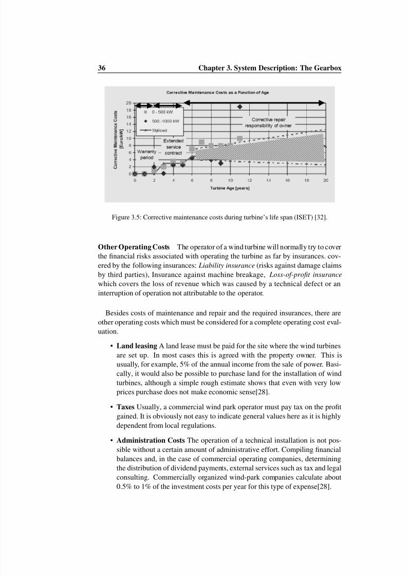
Figure 3.6: Gear Nomenclature
The following description considers gears in general with no particular focus onthe gearbox of a wind turbine. However it is assumed that most of the failuresmodes are similar to other applications where a gears are employed. Generallyspeaking, gearboxes and bearings can be affected by faults for the following mainreasons:
• Underestimated design loads;
• Torque Overloads;
• Wrong Material;
• Manufacturing errors;
• Damage during transportation and assembly;
• Misalignment of components in the shaft;
3.5.1 Fatigue Cracks
The most commonfailure mechanism 2.6.2 for gears is the Hertzian contact stress [25].It refers to the localized stresses that develop when two curved surfaces come incontact and deform slightly under loads. In gears and bearings in operation, thesecontact stresses are cyclic and over time lead to fatigue cracks[35] (Figure 3.7. Inthe AGMA standard it is claimed that if discovered early enough, many gear toothfailures can be avoided by proper corrective maintenance.
3.5.2 Teeth Breakage
Tooth cracking or breakage is the result of gear-tooth deterioration. Its existencein a gearbox indicates a situation already beyond the ability of maintenance toprevent the failure and the replacement of the component is the only possibility left

8/6/2019 Gearbox+ +Rossir24 0017
http://slidepdf.com/reader/full/gearbox-rossir24-0017 48/91
3.5. Failure Modes Analysis in Gears 39
Figure 3.7: Fatigue Cracks at the tooth root [35]
to retain the function of the gearbox. Fatigue breakage is the most common typeof failure by breakage[35]. It results from repeated bending stresses that are abovethe physical limits of the material. These types of stresses typically result from:
• Poor design;
• Overload;
• Misalignment;
• Tooth surface defects;
Breakage from heavy wear is a secondary type of failure, since it is a result of another kind of failure (i.e., wear). For instance, spalling or heavy abrasive wearcan remove enough metal to reduce the strength of the tooth below the breakingpoint. Overload breakage is a rather common type of failure resulting from suddenshock overload and does not show progression of the crack as in fatigue.Misalign-ment which concentrates the load at one end of the tooth face is usually the cause,but overload breakage also may be caused by bent shaft, or large pieces of particlesthe mesh.
This type of failure is prevented by protecting gears from extreme or transientloading. In Wind power industry this type of failure has been experienced dueto sudden shocks appearing on the generator side of the gearbox caused by shortcircuit or other faults in the generator [36].
3.5.3 Wear
Wear is a general term describing loss of material from the contacting surfaces of gear teeth[35].Levels of wear could be classied into: Light, Normal, Moderate
8/6/2019 Gearbox+ +Rossir24 0017
http://slidepdf.com/reader/full/gearbox-rossir24-0017 49/91
40 Chapter 3. System Description: The Gearbox
and Severe/Destructive. Light or Normal wear is part of the aging process of the
mechanical system and, as long the loss of metal occurs at a rate that do not affectperformances within the expected life of the gears wear do not represent a problem.In general, in order to reduce wear, a certain amount of smoothing and polishing isexpected during ”running in” of new gear sets. There exists different typologies of wear:
• Abrasive wear Surface injury caused by small particles through the gearmesh. These particles may be dirt not completely removed, sand or scalefrom castings, impurities in theoilor from thesurrounding atmosphere (dust,salt water), or metal detached from the tooth surfaces or bearings. TypicalMaintenance procedure in case of abrasive wear detection consists in stop-
ping the unit immediately and draining out the oil. A light ushing oil shouldbe used for a short time to remove particles from the gearbox(Figure 3.8,b)..
• Scratching Severe form of abrasive wear, characterized by lines that mayresemble scratches or marks on the contacting surfaces in the direction of sliding. It may be caused by defects on the tooth surface or material embed-ded in the tooth surface. It usually leads to light damage and does not resultin the progressive destruction of the component.
• Overload wear It is also a severe form of wear experienced under conditionsof heavy load and low speed, the metal seems to be removed progressivelyin the form of layers.
• Adhesive Wear it is dened as the action of one material sliding over anotherwith surface interaction and adhesion at localized contact areas, particularlyon the tooth top face (Figure 3.8,a).
3.5.4 Plastic Flow
Surface deformation resulting from the bending of the surface metal under heavyloads. It is usually caused by use of softer metals but it can occur with harder mate-rials. A gearbox replacement is usually required to correct plastic ow wear. Mostplastic ow wear and failures can be eliminated by reducing the contact stresses,and by increasing the hardness of the contacting surface material.
3.5.5 Scoring (Scufng)
Rapid removal of metal from the tooth surfaces caused by severe adhesion duringfrom metal-to-metal contact, characterized by transfer of metal from the surface of one tooth to that of another. Scufng is usually caused by the rupture of oil lmdue to excessive load. This type of wear can be reduced by increasing oil viscosity,or by reducing load or by smoothing the roughened area. Scufng can vary frommild to severe. Mild scufng is non progressive and therefore doesn’t constitute a

8/6/2019 Gearbox+ +Rossir24 0017
http://slidepdf.com/reader/full/gearbox-rossir24-0017 50/91
3.5. Failure Modes Analysis in Gears 41
Figure 3.8: Basic mechanisms of wear (adapted from [37])
primary failure in gears[38] Severe scufng occurs on gear teeth . In some cases,surface material is plastically deformed (3.5.4) and displaced over the tooth top orinto the tooth root. If not corrected, it is usually progressive.
3.5.6 Surface fatigue
It is the failure of the material as a result of continuous surface stresses. It is char-acterized by the removal of material and the formation of cavities. These cavitiesmay be small, they may be small at the beginning then increase size by continuedfatigue[35].Surface Fatigue can appear in different forms:
• Initial pitting . Surface fatigue which occur at the beginning of the opera-tional life and continue only until the overstressed local areas of the surfacehave been removed by polishing them. It is caused by local areas of highstress due to surfaces defects on the gear tooth.
• Destructive pitting . It usually start below the pitch line ( refer section 3.1),progressively increase size and number of pits destroying the tooth shape.The pits constitute stress raise which may lead to failure by fatigue breakage.Typical Maintenance procedures consist in grinding and polishing gear-toothsurface, or also extreme-pressure oil.

8/6/2019 Gearbox+ +Rossir24 0017
http://slidepdf.com/reader/full/gearbox-rossir24-0017 51/91
42 Chapter 3. System Description: The Gearbox
• Macropitting . It occurs when fatigue cracks start either at or below the sur-
face. As the cracks grow, they cause a piece of surface material to break out,forming a pit with sharp edges.
3.5.7 Spalling
. Fatigue failure occurring only in hardened steel, caused by surface defects orexcessive stresses due to heat treatment[35]. It is characterized by large particlesor chips that ake out the tooth surfaces. In hardened gears, it can leads to the lossof a single or several large areas of material. Typically gear manufacturer shouldbe contacted for reviewing the gears, its design and application[35].
8/6/2019 Gearbox+ +Rossir24 0017
http://slidepdf.com/reader/full/gearbox-rossir24-0017 52/91
Chapter 4
Condition Monitoring Systems in
Wind Turbine’s GearboxIn WindPowersystems CMSare rathernew technology but it is developingquickly.And indeed, it is state-of-the-art for onshore and offshore wind turbines to beequipped with vibration-based condition monitoring. Moreover, many insurancecompanies required wind turbines to be provided with an on-line CMS[39]. Forinstance, German insurer Allianz requires that all bearings in a drive train have tobe replaced after either 40,000 operating hours or ve years unless an appropriateCMS has been installed[4].
General benets arising from introducing a CMS(and a conditionbased-maintenanceprogramme) can be sum up in the following:
• Avoidance of premature breakdown . Early fault detection allows to pre-vent catastrophic failures to occur. For example, late detection of a bearingfault may in the worst case simply complete destruction of gearbox.
• Reduction of maintenance costs . By using on-line monitoring inspectionscan be avoided or inspection intervals increased.
• Supervision and Diagnosis at remote sites . Large wind turbines are usuallybuilt at remote sites where. On-line monitoring systems can detect suchchanges at an early stage and, if integrated in a network (section 4.3), send awarning and diagnostic details to the maintenance staff.
• Improvement of capacity factor . When a good estimation of the remaininguseful life is available, repairs or replacements action can be scheduled dur-ing time frames with no or little wind. Capacity factor is dened as the ratiobetween the actual production over a given period of time and the amount of power the turbine would have produced running at full capacity during thesame period of time [27].
43
8/6/2019 Gearbox+ +Rossir24 0017
http://slidepdf.com/reader/full/gearbox-rossir24-0017 53/91
44 Chapter 4. Condition Monitoring Systems in Wind Turbine’s Gearbox
• Support for further development . CMS provide detailed information on
the dynamic behavior of a wind turbine over long periods of time.The in-creased knowledge about the system can be used for supporting the designof wind turbine components.
Equipment parameters are a group of characteristics that indicate the state of the equipment condition. These characteristics, such as vibration, temperature areacquired by sensors placed in the relevant areas of the machine. Techniques forcondition monitoring have been successfully employed during the last decades indifferent industry such as marine propulsion or aerospace applications. Generalconsiderations and benets arising from use of condition monitoring are[14]:
• Condition monitoring does not prevent failures from happeningbut if failurescan be recognized at an early stage, appropriate measures can be taken tolimit the consequence damage;
• Maintenance actions can be better planned which leads to less unexpectedfailures and less downtime;
• Any measured data is useful for verication of the equipment design;
• Insurancecompaniesmayaskforregular inspections or conditionmonitoring[39];
The greatest benets from condition monitoring can be expected for offshorewind energy to change from corrective maintenance to condition based mainte-nance. In general, the actual condition of a machine can be measured and evaluatedeitherofine using mobile measurement equipment t, oronline using permanentlyinstalled sensors.The latter case is naturally the most suitable for offshore windfarms, where the accessibility to the site is usually more difcult and highly depen-dent on weather conditions.
Off-line monitoring requires that the wind turbine has to be shut down to allowinspection by maintenance personnel [2]. Generally inspections are scheduled atregular time intervals and consist of routine procedures and checklists. Off-line
monitoring is standard practice on commercial wind turbines. Scheduled mainte-nance generally includes(ISO 81400) :
• Levels and quality by analysis of oil samples;
• Inspection of bolts and joints;
• Measurement of wear items (bushings, seals);
• Special diagnostic techniques (methods for crack detection);
8/6/2019 Gearbox+ +Rossir24 0017
http://slidepdf.com/reader/full/gearbox-rossir24-0017 54/91
4.1. Vibration Analysis Techniques 45
On-line monitoring offers several advantages over off-line monitoring:
• Deeper insight into how well the turbine subsystems are performing whilerotating under load. ”Since maintenance personnel normally do not haveaccess to the turbine nacelle while the turbine is in operation, online con-dition monitoring is usually the only way for observing the turbine duringoperation [3]”.
• on-line monitoring can be incorporated into SCADA systems (section 4.3)to automatically trigger appropriate alarms and alert staff when a problemoccurs. It is especially useful in remote or inaccessible locations such as theoffshore turbines.
All commercial turbines incorporate basic on-line monitoring. Generally CMSincludes sensors to monitor machine parameters such as temperatures, uid levels,vibration (section 4.1).
As previously discussed, The question to ask when evaluating any of thesecondition monitoring systems is whether the cost of installing and commissioningthese systems is justied by its usefulness.The system must provide early enoughwarning to allow scheduling for repairs, but it must also provide information aboutthe system that cannot be estimated from routine visual inspection. It must alsobe considered that on-line CMS, if properly operating , can potentially reduce theman work costs for off-line inspections.
A breakdown in a bearing, normally ends up in a replacement of thecomplete gearbox. Without CM it is only ”the luck” that tells the main-tenance that something is happening in the mechanical condition inthe turbine. Secondary damages is often occurring in bearing housingand gears and shafts [13].
Another limitations in the use of continuous monitoring is that raw signals withnoise produces inaccurate diagnostic information. Periodic monitoring is, there-fore, used due to it being more cost effective and providing more accurate diag-nosis using ltered and or processed data. Of course, the risk of using periodicmonitoring is the possibility of missing some failure events which occur betweensuccessive inspections[11].
4.1 Vibration Analysis Techniques
Vibration analysis is the dominant technique used for predictive maintenance pro-grammes. This technique uses the noise or vibration created by mechanical equip-ment to detect machine problems. Thegear mesh frequency is the rate at whichgear teeth engage together in the pitch point (section 3.6) and it is equal to thenumber of teeth on the gear times the rpm of the gear. A gearbox always have a
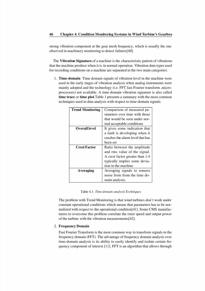
8/6/2019 Gearbox+ +Rossir24 0017
http://slidepdf.com/reader/full/gearbox-rossir24-0017 55/91
46 Chapter 4. Condition Monitoring Systems in Wind Turbine’s Gearbox
strong vibration component at the gear mesh frequency, which is usually the one
observed in machinery monitoring to detect failures[40].
TheVibration Signature of a machine is the characteristic pattern of vibrationsthat the machine produce when it is in normal operation. Vibration data types usedfor recording conditions on a machine are separated in the two main categories:
1. Time-domain Time domain signals of vibration level in the machine wereused in the early stages of vibration analysis when analog instruments weremainly adopted and the technology (i.e. FFT fast Fourier transform ,micro-processors) not available. A time-domain vibration signature is also calledtime trace or time plot .Table 1 presents a summary with the most common
techniques used in data analysis with respect to time-domain signals.Trend Monitoring Comparison of measured pa-
rameters over time with thosethat would be seen under nor-mal acceptable conditions
Overall level It gives some indication thata fault is developing when itreaches the alarm level that hasbeen set
Crest Factor Ratio between the amplitude
and rms value of the signal.A crest factor greater than 1.4typically implies some devia-tion in the machine
Averaging Averaging signals to removenoise from from the time do-main analysis.
Table 4.1:Time domain analysis Techniques
The problem with Trend Monitoring is that wind turbines don’t work underconstant operational conditions which means that parameters has to be nor-malized with respect to the operational condition[41]. Some CMS manufac-turers to overcome this problem correlate the rotor speed and output powerof the turbine with the vibration measurements[42].
2. Frequency Domain
Fast Fourier Transform is the most common way to transform signals in thefrequency domain (FFT). The advantage of frequency domain analysis overtime-domain analysis is its ability to easily identify and isolate certain fre-quency component of interest [11]. FFT is an algorithm that allows through

8/6/2019 Gearbox+ +Rossir24 0017
http://slidepdf.com/reader/full/gearbox-rossir24-0017 56/91
4.1. Vibration Analysis Techniques 47
a signal processor to evaluate the Fourier transform of a periodic signal. Fre-
quency domain analysis is often applied in gearboxes and bearings becauseeach component and its associated failure modes in rotating machinery arecharacterized by a determined frequency[38]. Among different techniquesbased on frequency domain, one the most effective to detect failures for bear-ings in a early stage is theShock Pulse Method . A high frequency pressurewave (typically 36 kHz) is applied on the metal surface[42]. The amplitudeof the shock is proportional to the condition of metal-to-metal contact sur-faces Specic accelerometers and lters are needed to measure such signals.JanHoin
Functional Failure
Heat Generation
Wear Particle oilChanges in vibrations
Audible noise
P
F
Time
C o n
d i t i o n
Figure 4.1:
A further classication for vibration analysis techniques is the following:
• Broadband trending
This technique acquires overall vibration readings from select points on themachine. These data are compared with either a baseline reading taken froma new machine to determine the relative condition of the machine. Normallythis measurement provides total vibration energy between 10 and 10,000 Hzand therefore it is only providing information on the overall state of the com-ponent not giving any information about failure modes. Specic machineproblems cannot be isolated and identied.
• Narrowband trending
Differently from broadband, narrow brand trending analysis uses only vi-bration frequencies that represent specic machine components or failuremodes. This method provides the ability to monitor the condition of gearwheels, and bearings.
In the Wind Power industry, Vibration monitoring is used to detect faults in thebearings and gears. Sensors are mounted to the bearing housing or gear case to
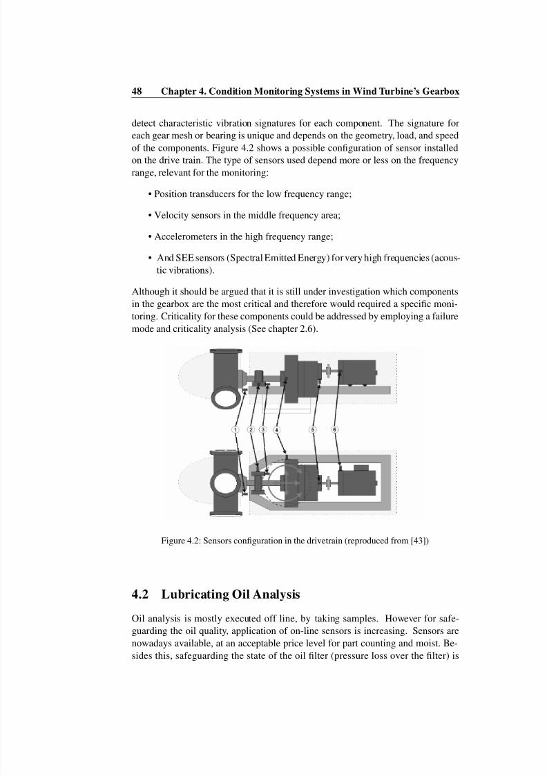
8/6/2019 Gearbox+ +Rossir24 0017
http://slidepdf.com/reader/full/gearbox-rossir24-0017 57/91
48 Chapter 4. Condition Monitoring Systems in Wind Turbine’s Gearbox
detect characteristic vibration signatures for each component. The signature for
each gear mesh or bearing is unique and depends on the geometry, load, and speedof the components. Figure 4.2 shows a possible conguration of sensor installedon the drive train. The type of sensors used depend more or less on the frequencyrange, relevant for the monitoring:
• Position transducers for the low frequency range;
• Velocity sensors in the middle frequency area;
• Accelerometers in the high frequency range;
• And SEEsensors (SpectralEmitted Energy) forvery high frequencies (acous-
tic vibrations).Although it should be argued that it is still under investigation which componentsin the gearbox are the most critical and therefore would required a specic moni-toring. Criticality for these components could be addressed by employing a failuremode and criticality analysis (See chapter 2.6).
Figure 4.2: Sensors conguration in the drivetrain (reproduced from [43])
4.2 Lubricating Oil Analysis
Oil analysis is mostly executed off line, by taking samples. However for safe-guarding the oil quality, application of on-line sensors is increasing. Sensors arenowadays available, at an acceptable price level for part counting and moist. Be-sides this, safeguarding the state of the oil lter (pressure loss over the lter) is
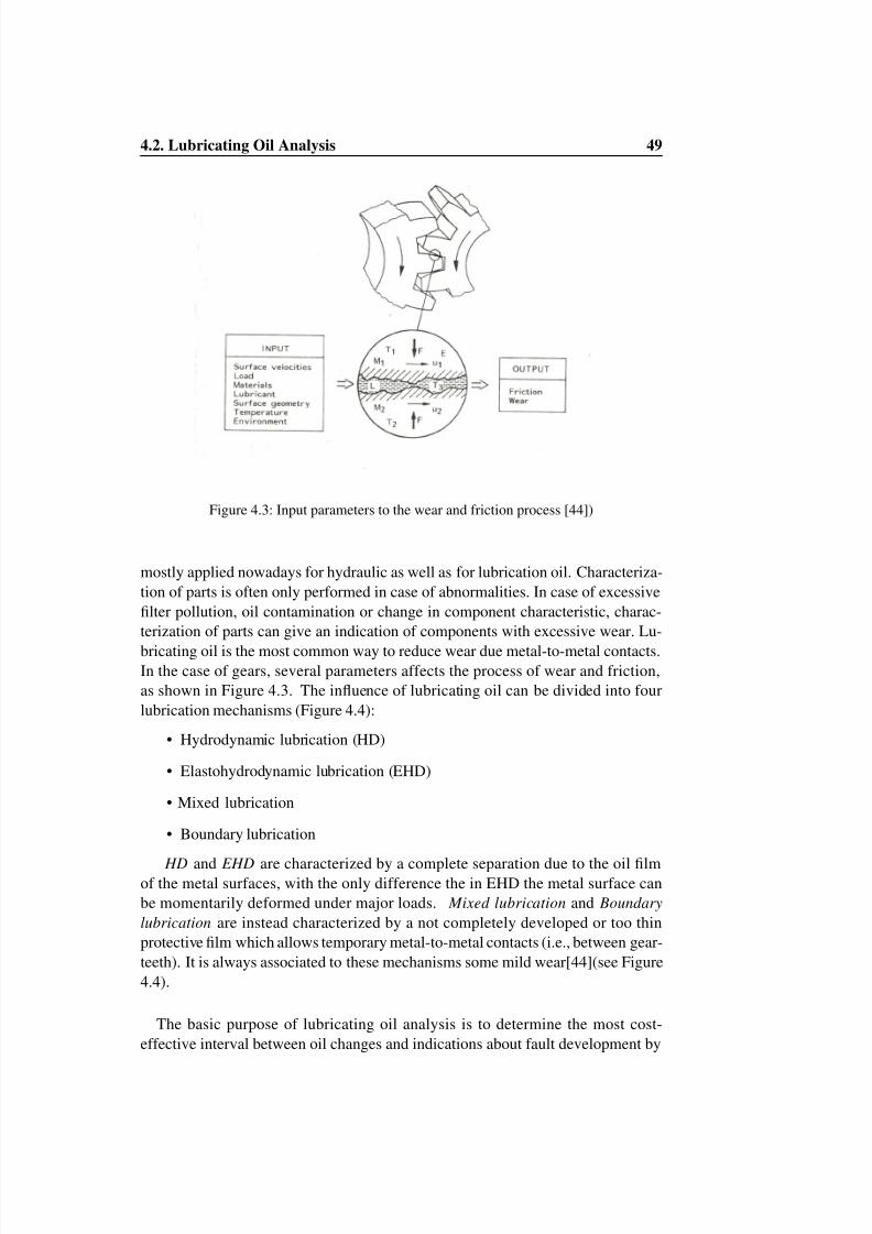
8/6/2019 Gearbox+ +Rossir24 0017
http://slidepdf.com/reader/full/gearbox-rossir24-0017 58/91
4.2. Lubricating Oil Analysis 49
Figure 4.3: Input parameters to the wear and friction process [44])
mostly applied nowadays for hydraulic as well as for lubrication oil. Characteriza-tion of parts is often only performed in case of abnormalities. In case of excessivelter pollution, oil contamination or change in component characteristic, charac-terization of parts can give an indication of components with excessive wear. Lu-bricating oil is the most common way to reduce wear due metal-to-metal contacts.In the case of gears, several parameters affects the process of wear and friction,as shown in Figure 4.3. The inuence of lubricating oil can be divided into fourlubrication mechanisms (Figure 4.4):
• Hydrodynamic lubrication (HD)
• Elastohydrodynamic lubrication (EHD)
• Mixed lubrication
• Boundary lubrication
HD and EHD are characterized by a complete separation due to the oil lmof the metal surfaces, with the only difference the in EHD the metal surface canbe momentarily deformed under major loads.Mixed lubrication and Boundarylubrication are instead characterized by a not completely developed or too thinprotective lm which allows temporary metal-to-metal contacts (i.e., between gear-teeth). It is always associated to these mechanisms some mild wear[44](see Figure4.4).
The basic purpose of lubricating oil analysis is to determine the most cost-effective interval between oil changes and indications about fault development by
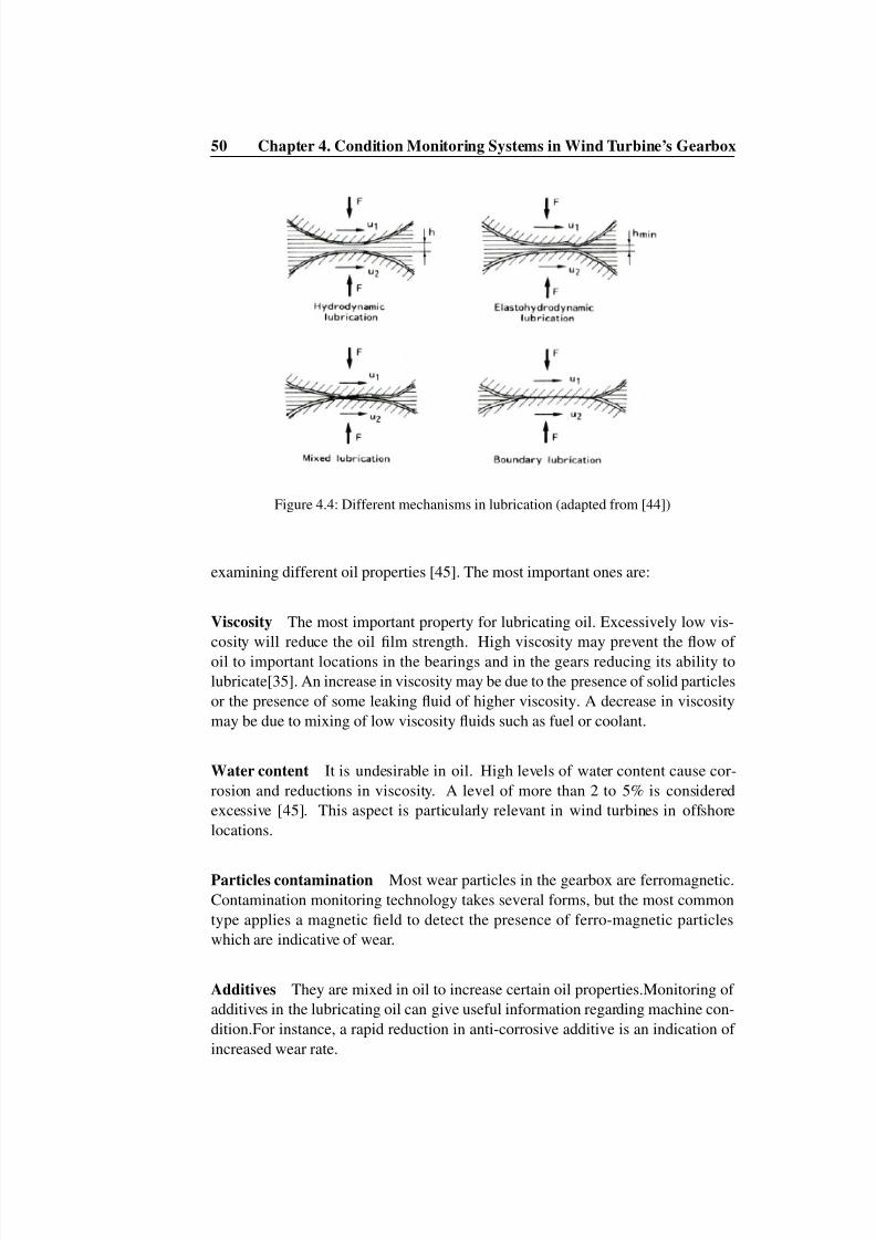
8/6/2019 Gearbox+ +Rossir24 0017
http://slidepdf.com/reader/full/gearbox-rossir24-0017 59/91
50 Chapter 4. Condition Monitoring Systems in Wind Turbine’s Gearbox
Figure 4.4: Different mechanisms in lubrication (adapted from [44])
examining different oil properties [45]. The most important ones are:
Viscosity The most important property for lubricating oil. Excessively low vis-cosity will reduce the oil lm strength. High viscosity may prevent the ow of oil to important locations in the bearings and in the gears reducing its ability tolubricate[35]. An increase in viscosity may be due to the presence of solid particlesor the presence of some leaking uid of higher viscosity. A decrease in viscositymay be due to mixing of low viscosity uids such as fuel or coolant.
Water content It is undesirable in oil. High levels of water content cause cor-rosion and reductions in viscosity. A level of more than 2 to 5% is consideredexcessive [45]. This aspect is particularly relevant in wind turbines in offshorelocations.
Particles contamination Most wear particles in the gearbox are ferromagnetic.Contamination monitoring technology takes several forms, but the most commontype applies a magnetic eld to detect the presence of ferro-magnetic particleswhich are indicative of wear.
Additives They are mixed in oil to increase certain oil properties.Monitoring of additives in the lubricating oil can give useful information regarding machine con-dition.For instance, a rapid reduction in anti-corrosive additive is an indication of increased wear rate.
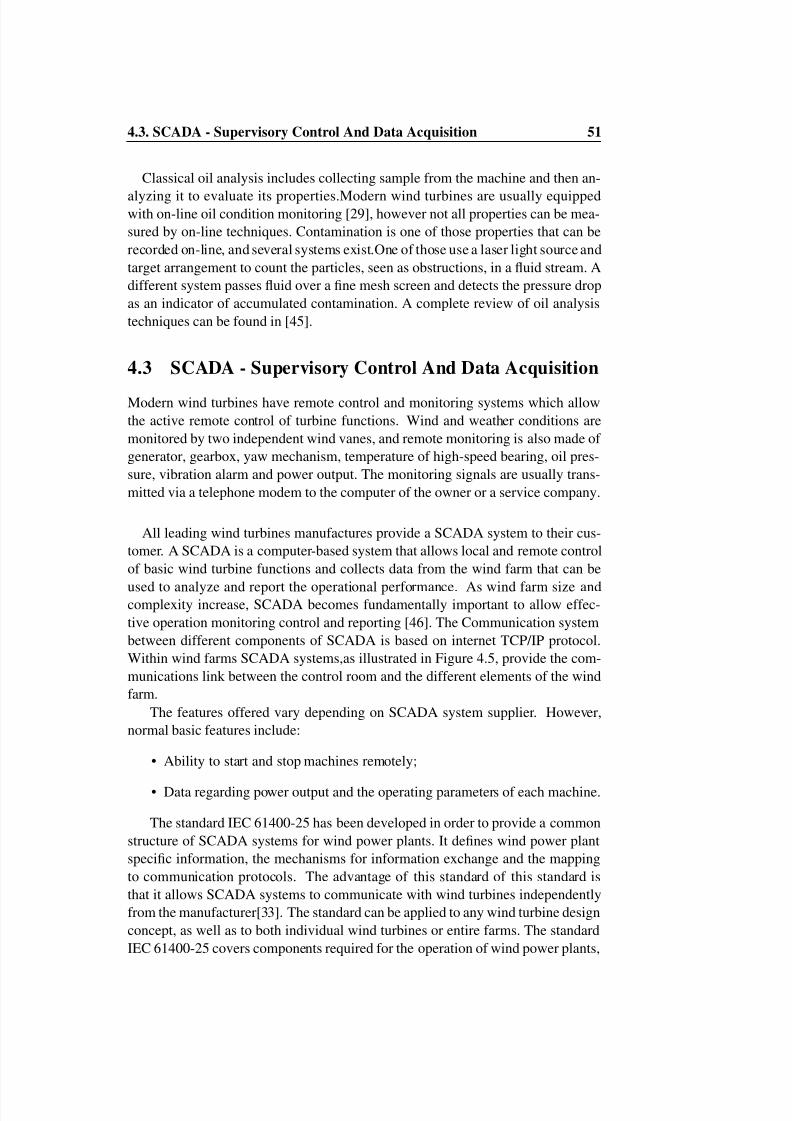
8/6/2019 Gearbox+ +Rossir24 0017
http://slidepdf.com/reader/full/gearbox-rossir24-0017 60/91
4.3. SCADA - Supervisory Control And Data Acquisition 51
Classical oil analysis includes collecting sample from the machine and then an-
alyzing it to evaluate its properties.Modern wind turbines are usually equippedwith on-line oil condition monitoring [29], however not all properties can be mea-sured by on-line techniques. Contamination is one of those properties that can berecorded on-line, and several systems exist.One of those use a laser light sourceandtarget arrangement to count the particles, seen as obstructions, in a uid stream. Adifferent system passes uid over a ne mesh screen and detects the pressure dropas an indicator of accumulated contamination. A complete review of oil analysistechniques can be found in [45].
4.3 SCADA - Supervisory Control And Data Acquisition
Modern wind turbines have remote control and monitoring systems which allowthe active remote control of turbine functions. Wind and weather conditions aremonitored by two independent wind vanes, and remote monitoring is also made of generator, gearbox, yaw mechanism, temperature of high-speed bearing, oil pres-sure, vibration alarm and power output. The monitoring signals are usually trans-mitted via a telephone modem to the computer of the owner or a service company.
All leading wind turbines manufactures provide a SCADA system to their cus-tomer. A SCADA is a computer-based system that allows local and remote controlof basic wind turbine functions and collects data from the wind farm that can be
used to analyze and report the operational performance. As wind farm size andcomplexity increase, SCADA becomes fundamentally important to allow effec-tive operation monitoring control and reporting [46]. The Communication systembetween different components of SCADA is based on internet TCP/IP protocol.Within wind farms SCADA systems,as illustrated in Figure 4.5, provide the com-munications link between the control room and the different elements of the windfarm.
The features offered vary depending on SCADA system supplier. However,normal basic features include:
• Ability to start and stop machines remotely;
• Data regarding power output and the operating parameters of each machine.
The standard IEC 61400-25 has been developed in order to provide a commonstructure of SCADA systems for wind power plants. It denes wind power plantspecic information, the mechanisms for information exchange and the mappingto communication protocols. The advantage of this standard of this standard isthat it allows SCADA systems to communicate with wind turbines independentlyfrom the manufacturer[33]. The standard can be applied to any wind turbine designconcept, as well as to both individual wind turbines or entire farms. The standardIEC 61400-25 covers components required for the operation of wind power plants,

8/6/2019 Gearbox+ +Rossir24 0017
http://slidepdf.com/reader/full/gearbox-rossir24-0017 61/91
52 Chapter 4. Condition Monitoring Systems in Wind Turbine’s Gearbox
Figure 4.5: SCADA components in wind farms (reproduced from [46])
i.e. the wind turbine generator, the meteorological system, the electrical systemand the control unit.
SCADA can be utilized both by the manufacturer and by operators for efcientlycontrolling the the system and identifying problems. However one of the limitationof utilize a SCADA system, especially when integrated with CMS is that a greatamount of data is acquired and it can become very complex to manage them.

8/6/2019 Gearbox+ +Rossir24 0017
http://slidepdf.com/reader/full/gearbox-rossir24-0017 62/91
Chapter 5
Including CMS data in
Maintenance ModelingIn the previous chapter we have shown some of the most common modeling meth-ods for optimizing replacement and inspection times. The limitations of such mod-els were discribed when considering equipment whom condition can be monitored.The main idea in this chapter is to introduce techniques which allow the inclusionof condition monitoring data recorded either continously or at during inspectiontimes. The main approach consists in introducing the proportional hazards model(PHM) for maintenance optimization. The PHM is basically a regressionj modelfor life data tables which included the effects of so-called covariates which are de-ned as stressors and explenatory varialbles assumed to inuence the life of thecomponent under study.
5.1 Basic Concepts
5.1.1 Hazard Rate
Let T represent the survival time. The hazard rate, also called failure rate or forceof mortality, is dened as:
z(t ) = lim∆ t→ 0
P [(t ≤ T < t + ∆ t) | T ≥ t ]∆ t
(5.1)
The failure rate is dened for a non repairable component as the instantaneousrate of failure of a functioning component at time t during the next instant of time.The failure rate is sometimes called a "conditional failure rate". The probabilityP that a component that survived until time t will still be functioning after a timeinterval∆ t is approximately z(t)*∆ t .
53

8/6/2019 Gearbox+ +Rossir24 0017
http://slidepdf.com/reader/full/gearbox-rossir24-0017 63/91
54 Chapter 5. Including CMS data in Maintenance Modeling
5.1.2 Failure times and Sunspensions
Reliability data are evaluated based on the use of Reliability Database (see Chapter6.1), on expert jusdgment or on operational data which mainly consist of failuredata. If the actual lifetime of every item in the sample is recorded, the data arecalled complete data. When not all items in the sample have failed at the time of observation the data are called incomplete data. This type of data are also calledcensored. Operational Data are often censored. If for example, due to preventivemaintenance, a functioning component is replaced preventevely, we considered thatitem as censored.
Any large component undergoes under major or minor repairs. Major repairsare typically considered as renewal in the way that the component may be consid-ered in as good as new state. For minor repairs the situation is more complex andmay be decided on single cases. Typical examples of rapairs carried on the gearboxare:
Table 5.1: Different Forms of Event Data - Maintenance actions on a gearbox1. An oil change2. A rotor balance3. A shaft/coupling alignment4. Tightning, calibration, minor adjustments that affect the condition data5. A lter replacement
5.1.3 Covariates
A covariate is dened as a treatment or explanatory variable that inuences thefailure time of the component. A vector of covariates
x = {x1, x 2,...,x n }
is chosen and each entry of the vector represents a unique explanatory vari-able. Typical covariates include those that represent mechanical forces, materialproperties, and environmental variables. In Section 4.1 we have described differ-ent tecniques used for monitoring condition of the gearbox. CMS, CMMS and
SCADA provide to the user a large amount of information which can be deneby nature as covariates inuencing the gearbox life time. Covariates can either beconstant or dependent of time. Examaples of covariates of interest may be:
Oil Analysis Contamination in lubrication oil, expressed by example in iron con-tamination ppm (parts per milion).
Vibration Measurements Amplitude of vibrations signals on bearings, gearboxcase, etc.Covariates for vibration measurements can for example be the averageamplitude over a specic frequency bands relevant for a failure mode

8/6/2019 Gearbox+ +Rossir24 0017
http://slidepdf.com/reader/full/gearbox-rossir24-0017 64/91
5.1. Basic Concepts 55
Mechanical Loading It could for example be expressed as fraction of the power
production, proportial to the wind speed and thus the mechanical trust on the gears.Although, tipically output power is already integrated in the CMS data sincethevibration noise level is proportional to the rpm of the gearbox.
Furhtermore, explanatory variables could be used to take in account differ-ent environmental conditions.Covariates should be identied for each failure modesince the dynamic of each failure mode is different. Experts in condition monitor-ing should give a list of potential covariates; some may be dropped if they are notsignicant. Time dependent covariates falls in two broad classications [47]:
External : Covariate that is not directly involved with the failure mechanism.Typical examples may be the operating temperature or other type of environmentalfactors.
Internal : Time measurement taken on the the component.The oberved covari-ate’s value carries information about the surival time of the corresponding individ-ual. Given that an internal covariate z(t) doesn’t indicate a failure, it follows fromth denition of R (t, x ) = P (T ≥ t | x (t ), β ) = 1 . External covariates may beclassied in the following subgroups [47] :
• Fixed Measured in advance and xed for the duration of observation
• Dened No constant but determined in advance for each component understudy.
• Ancillary External to the component and with stochastic behavior
Table 5.2: FMECA carried out for the CONMOW project [41].
Table 5.2 shows a potential FMECA for the gearbox. In order to assess critical-ity of each failure mode, a severity class has been developed. The table illustrates

8/6/2019 Gearbox+ +Rossir24 0017
http://slidepdf.com/reader/full/gearbox-rossir24-0017 65/91
56 Chapter 5. Including CMS data in Maintenance Modeling
which failure modes can be detected by vibrations analysis (CM-1).The severity
classes are instead dened: Replacement of large components (F6), service withreplacement (F5) and "Alarm with repair" (F2) which means that the turbine willshut down due to the alarm and a remote reset is not the appropriate means to restartthe turbine. A visit from a technician is required. In this failure class, a toolboxwith small spare parts and consumables is sufcient to carry out the repair.
Covariates should be identied for each failure mode since the dynamic of eachfailure mode is different. Experts in condition monitoring should give a list of potential covariates; some may be dropped if they are not signicant.
5.2 Proportional Hazards ModelThe Proportional Hazards Model is the most used and cited model which incor-porate the effect of covariates on the distributions of life times. It was orginallydeveloped by Cox (1975)[48] and further applied in several applications amongwhich, maintenance. It is a widely accepted semi-parametric model for analysis of failures with covariates. The general expression of the PHM:
z(t, x ) = z0(t ) · eβ T x (5.2)
It is easy to see that forβ = 0 there is not correlation between the covariatesand the life time of the component.
Cumulative Hazard Rate The relation between the hazard rate and the cumula-tive hazard rate is given by:
z(t ) =ddt
Z (t )
from which it follows:
Z (t, x ) = t
0z(u, x ) du =
t
0z0(u )eβ T x du = eβ T x
t
0z0(u ) du = Z 0(t) ·eβ T x
(5.3)
The probability density function is given by:
f (t, x ) = z(t, x ) · exp {− t
0z(u, x ) du} = z0(t ) · eβ T x · exp {eβ T x
t
0z0(t ) du}

8/6/2019 Gearbox+ +Rossir24 0017
http://slidepdf.com/reader/full/gearbox-rossir24-0017 66/91
5.2. Proportional Hazards Model 57
Reliability function Using the previous relation we easily evaluate also the reli-
ability function:
R (t, x ) = e− Z (t,x ) = e− Z 0 (t )exp (β T x) = [R 0(t )]exp (β T x)
whereR 0(t ) is the reliability function for theWeibullDistribution. Thestrenghtand success of PHM is given by the fact that it is possible to estimate a relative riskof failure also when we ignore the real life distribution of failures. We may wantinvestigate what is the inuence of oil contamination on the lifetime of the compo-nent for two given different covariates value x and x. The relative risk is thus:
z0(t ) · eβ T x
z0(t ) · eβ T x = eβ T (x− x )
This statistical model is called proportional hazards method because the sur-vivatl of the component is proportional to the covariate effects, as shown in Figure. The use of xed covariates in maintenance application is questionable. All theinput CMS until here described are time dependent and internal, their exsitance isdependent upon the functioning state of the equipment under study.
5.2.1 Baseline hazard rate
The hazard rate z(t,x) is composed by a time dependent part and a part dependenton the covariates. In the original Cox [48] model the baseline hazard function isunspecied, and thus the model a semi-parametric (only the covariates vector isestimated). The baseline hazard ratez0(t ) may be calculated, depending on theβ vector, by non-parametric analysis (See Appendix A). A fully parametric approachcan also be used. In this case, the baseline hazard rate can be freely choose amnongany distribution famlily and the inference on parameters may be obtained by theclassical maximul likelihood approach (see, [8]). In maintenance application, itis common the use of Weibull distribution for the simple reason that it is possibleto model different type of aging by modifying the shape parameter. The densityfunction for a Weibull distribution with scale parameterλ and shape parameterα
f 0(t ) =αλ
tλ
α − 1e− ( t
λ )α for t>0
and hazard rate:
z0(t ) =αλ
·tλ
α − 1
Model with time dependent covariates The natural exstension for includingtime dependent covariates:
z(t, x ) = z0(t ) · eβ T x(t) (5.4)

8/6/2019 Gearbox+ +Rossir24 0017
http://slidepdf.com/reader/full/gearbox-rossir24-0017 67/91
58 Chapter 5. Including CMS data in Maintenance Modeling
In the Cox proportional hazards model, the ratio of hazard functions for any
two components is assumed to be independent of time t. However, it is common inpractice that study include both time-dependent and time-independent covariates.For example, the size of a wind turbine, or the environmental condition under oper-ation do not change. Other variables, such as data acquired by the CMS vary withtime and are often collected in subsequent examinations, or even continously. Thepartial likelihood function allowing time-dependent covariates has the same formas that in Appendix-A except now the covariates are dependent on time:
L (β ) =m
i=1
eβ T x j (t j )
m j =1 eβ T x j (t j )
(5.5)
β x βx
H A Z A R D
R A T E
Timet 2t 1
TT
Effects of covariates
Observed Hazard rate
Baseline Hazard Rate
Figure 5.1: Effects of covariates on the reliability function
5.3 Model Building
5.3.1 Input Data
Themodelaccuracydepends on thequality andquantity of data collected. Condition-monitoring data is quite often available in large quantities because most industrialplants today have regular CBM program. On the other hand, failure data is oftenlacking or inadequate.
1. failure/replacement data;
2. inspection data;
3. maintenance action data;
Necessary event data are condition monitoring data (i.e, covariate values) andfailure data for each failure mode including the age of the equipment. Typicallydata are shown in the form(t i , δi , x i (t i)) , the triplete indicating the failure time,the censoring variable and the value of covariates vector at failure.

8/6/2019 Gearbox+ +Rossir24 0017
http://slidepdf.com/reader/full/gearbox-rossir24-0017 68/91
5.4. Cost model and optimization 59
It is important to observe thatz(t | {X (t ) = x (t ); t ≥ 0)}, β )d t is approxi-
mately the probability that T lies in the interval [t, t +dt), conditioned ont ≥ T andX (t ) = x (t ) (see 5.1.1).
5.3.2 Parameter Estimation
The basic parameters to be calculated in the PHM are the coefcients of the covari-ates vectorβ . The maximum partial likelihood method is used to estimate theseparametes. See Appendix A for details on the parameters estimation. The generalformula is:
L (β ) =
m
i=1
exp β T x i
l∈R iexp β T
j x l(5.6)
where m is the number of failures, and R the set risk at the time of them th fail-ure. The estimation of β is sufcient so that the relative risk can be estimated.Thebaseline hazard rate may be estimated by the approach presented in the appendixand may be found in [49]
5.3.3 Model Testing
Once the vectorβ is estimated, Goodness-of-Fit tests may be used to test if the se-lected model is statistically signicant. The Kolmogorov-Smirnov test (Chakravart,Laha, and Roy, 1967) ,also implemented in the EXAKT has the advantage that thedistribution of the K-S test statistic itself does not depend on the underlying cumu-lative distribution function being tested. Furthermore, statistical hypothesis testingcan be used to verify that a covariate is signicant, i.e. if it has inuence on thelifetime of the component. The likelihood ratio test is one of the most used, furtherreadings may be found in [48]. The test statistic is thus:
W = 2( l(β − l(0)) ≈ χ 21
where l indicates the log-likelihood andβ the estimated covariates vector.Other test statistics may be utilized. Refer to Ansell (1994)[49] for further reading.
5.4 Cost model and optimization
The approach presented in this section has been proposed by Jardine [17]. TheProportional Hazard model is modied by considering time dependent covariates.The failure rate obtained by PHM is used in the age replacement policy describedin section 2.5.1:
The total cost per unit of time is a function of the risk level d, i.e. the risk leveldependent on time and covariates level at which the component replacement or amajor repair is required.

8/6/2019 Gearbox+ +Rossir24 0017
http://slidepdf.com/reader/full/gearbox-rossir24-0017 69/91
60 Chapter 5. Including CMS data in Maintenance Modeling
C (d) = C + K · Q (d)W (d)
(5.7)
T is dened as the time to faiure of the system. Q(d) Probability that failurereplacement will occur and it is dened as:
Q (d) = P (T d ≥ T )W(d) is the expected time between replacement regardeless if it is due to a
planned or unscheduled replacement as a function of the risk level.
W (d) = E (min {T d , T })
Covariates are time dependent and observed at equidistant discrete times andthe replacement decision may be done at any time in the transition. The covariatedynamic is described by a Markov chain. It should be noted that a Markov modelassume implicitly that the dynamic is without trends while, in the case of a windturbine, the load varies constantly. It has been proved in (theorem 2, [50]) that theoptimal replacement policy has the form:
T d = inf {t > 0 : K · z (t, X t ) ≥ d}The optimal d, noted d* minimizes the average cost function
g(d) = C (d) =C + K · Q (d)
W (d) (5.8)
A method for calculating d* is to calculate the sequence{xn } dened by:xn +1 = g(x n )
xn will converge to d* because g(d) is a convex function and d* its minimum(Proof in [50], theorem 4).The initial value of x0 may be guessed or chosen ran-domly. The sequence is stopped wheng(xn ) = g(x n − 1). d* is the optimal risklevel and optimal average cycle cost. To computexn , g(d) needs to be calculated.P (T d > = T )] and E [min (T, T d)] can be calculated using a recursive methodbased on the discretization of the covariate state space. The method is presented
in [50]. This algorithm is implemented in EXAKT[51] a software for optimizingcondition based maintenance by the use of PHM. Once the optimal risk leveld∗ isdetermined the item is replaced at time t so that
αλ
tλ
α − 1exp (βx (t )) ≥
d∗
K =
β 1 · x1(t )... · β n x n (t) ≥ φ(t ) =d∗λ α
Kα− (α − 1)lnt
φ(t ) is alo referred as warning-limit function. For the values, either time orcovariates, the area overφ(t ) indicates an immidiate replacemente and viceversa.
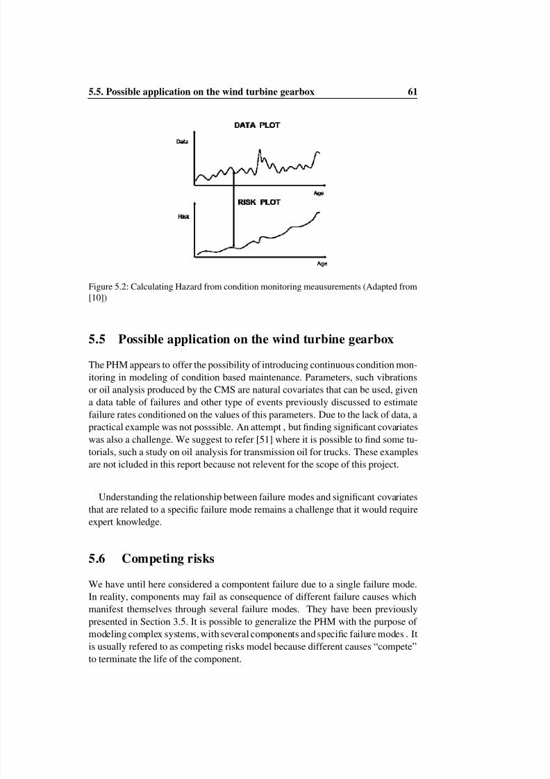
8/6/2019 Gearbox+ +Rossir24 0017
http://slidepdf.com/reader/full/gearbox-rossir24-0017 70/91
5.5. Possible application on the wind turbine gearbox 61
Figure 5.2: Calculating Hazard from condition monitoring meausurements (Adapted from[10])
5.5 Possible application on the wind turbine gearbox
The PHM appears to offer the possibility of introducing continuous condition mon-itoring in modeling of condition based maintenance. Parameters, such vibrationsor oil analysis produced by the CMS are natural covariates that can be used, givena data table of failures and other type of events previously discussed to estimatefailure rates conditioned on the values of this parameters. Due to the lack of data, apractical example was not posssible. An attempt , but nding signicant covariateswas also a challenge. We suggest to refer [51] where it is possible to nd some tu-torials, such a study on oil analysis for transmission oil for trucks. These examplesare not icluded in this report because not relevent for the scope of this project.
Understanding the relationship between failure modes and signicant covariatesthat are related to a specic failure mode remains a challenge that it would requireexpert knowledge.
5.6 Competing risks
We have until here considered a compontent failure due to a single failure mode.In reality, components may fail as consequence of different failure causes whichmanifest themselves through several failure modes. They have been previouslypresented in Section 3.5. It is possible to generalize the PHM with the purpose of modeling complex systems, withseveral components andspecic failure modes . Itis usually refered to as competing risks model because different causes “compete”to terminate the life of the component.
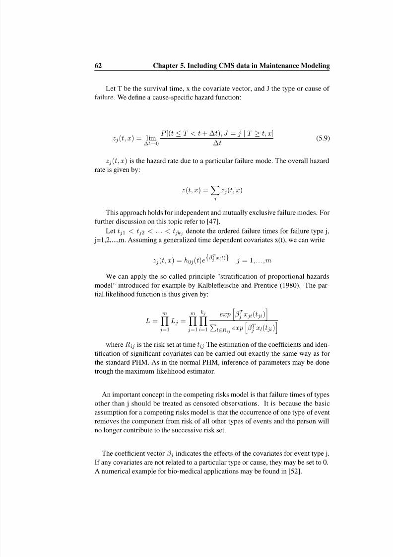
8/6/2019 Gearbox+ +Rossir24 0017
http://slidepdf.com/reader/full/gearbox-rossir24-0017 71/91
62 Chapter 5. Including CMS data in Maintenance Modeling
Let T be the survival time, x the covariate vector, and J the type or cause of
failure. We dene a cause-specic hazard function:
z j (t, x ) = lim∆ t→ 0
P [(t ≤ T < t + ∆ t ), J = j | T ≥ t, x ]∆ t
(5.9)
z j (t, x ) is the hazard rate due to a particular failure mode. The overall hazardrate is given by:
z(t, x ) = j
z j (t, x )
This approach holds for independent and mutually exclusive failure modes. Forfurther discussion on this topic refer to [47].
Let t j 1 < t j 2 < ... < t jk j denote the ordered failure times for failure type j, j=1,2,...,m. Assuming a generalized time dependent covariates x(t), we can write
z j (t, x ) = h 0 j (t)e{β T j x ( t )} j = 1 ,...,m
We can apply the so called principle "stratication of proportional hazardsmodel“ introduced for example by Kalbleeische and Prentice (1980). The par-tial likelihood function is thus given by:
L =m
j =1L j =
m
j =1
kj
i=1
exp β T j x ji (t ji )
l∈R ijexp β T
j x l(t ji )
whereR ij is the risk set at timet ij The estimation of the coefcients and iden-tication of signicant covariates can be carried out exactly the same way as forthe standard PHM. As in the normal PHM, inference of parameters may be donetrough the maximum likelihood estimator.
An important concept in the competing risks model is that failure times of typesother than j should be treated as censored observations. It is because the basicassumption for a competing risks model is that the occurrence of one type of eventremoves the component from risk of all other types of events and the person willno longer contribute to the successive risk set.
The coefcient vectorβ j indicates the effects of the covariates for event type j.If any covariates are not related to a particular type or cause, they may be set to 0.A numerical example for bio-medical applications may be found in [52].

8/6/2019 Gearbox+ +Rossir24 0017
http://slidepdf.com/reader/full/gearbox-rossir24-0017 72/91
5.7. Remarks on the use of PHM 63
5.7 Remarks on the use of PHM
Condition monitoring is not actually monitoring the equipment’s condition per se,but variables that it is assumed to be related to it. Those covariates, or variables,that inuence the probability of failure as shown in equation 5.2. From the modelwe want learn how each covariate inuences the reliability of the system, to makepredictions based on the past data [10].
The rst limatation of this approach is that data may not be available or onlyavailable within industry. A limited applicability of this model is caused by thescarce knowledge about failure modes and their relationship with observed covari-ates.
Furthermore, as previously discusssed, the assumption of covariates behaviourdescribed by a time homogenous markov chain may not be appropriate in the caseof failure occurences due to sudden shocks and large variability of mechanicalloads on the gearbox.

8/6/2019 Gearbox+ +Rossir24 0017
http://slidepdf.com/reader/full/gearbox-rossir24-0017 73/91

8/6/2019 Gearbox+ +Rossir24 0017
http://slidepdf.com/reader/full/gearbox-rossir24-0017 74/91
Chapter 6
Routines for Data Collection
Data and information about the system are the primary input for reliability analysis.This chapter gives an introduction to the process involved in collecting failure data.The input data can be derived from expert judgments or on experience data fromdifferent installations. Generic reliability database have been develop, we will herefocus on the OREDA database.
6.1 The OREDA project
The OREDA [53] project has started in 1981 by SINTEF in co-operation with the
Norwegian Petroleum Directorate and its main objective is ”to contribute to animproved safety and cost effectiveness in design and operation“ in the Oil and Gasindustry by establishing a RAMS database. The oil companies have systematicallycollected reliability data for more than 25 years.
The data in OREDA is collected through eld experience in several windows anare updated as one obtains additional information on failure rates so forth. The datapresented in the handbook is collected, and compared, across numerous platformsand installations and this forces the handbook to deal with the problem of non-homogeneity in the failure data. The Reliability data is given in equipment classesand then subdivided into two lower levels called sub-units and maintenable items.The failure are further subdivided into three categories:
1. Critical: A Failure that causes immediate and complete loss of a system’scapability of providing the demanded output.
2. Degraded: A failure that is not critical, but prevents the system from op-timal performance. Such failure may develop into a critical failure if leftunattended.
3. Incipient: A failure that at the moment does not cause any problems with re-spect to performance, but which may Develop into one of the failures aboveif left unattended.
65

8/6/2019 Gearbox+ +Rossir24 0017
http://slidepdf.com/reader/full/gearbox-rossir24-0017 75/91
66 Chapter 6. Routines for Data Collection
OREDA bases the calculation on the assumption of a constant failure rate which
is thus time independent. This implies thatλ (t ) = λ . However, as the handbookclearly states there has been no statistical tests to verify the assumption of theconstant failure rate. The failure rates in the handbook are based on at part of thebathtub curve and will therefore underestimate the actual failure rates.
In some cases the failure data in OREDA are collected on the basis of identicalitems which have been in operation under the same functional and environmentalconditions and it is then common to make the assumption of homogeneity. Theestimator for the failure rate can then be given by
λ =Number of failures
Aggregated time in service=
n
τ
(6.1)
Homogeneous Sample The calculation in OREDA are based on the assumptionof constant failure rate. In the handbook is also stated that infant mortality (i.e, thedecreasing part of the bath tube curve ) has not been considered. This is due tothe fact that often components are thoroughly tested before they are put in opera-tion. It is also assumed that failure data are taken from identical items operatingunder the same environmental condition. If several components has experiencedthe same failure rateλ or failures of a single item shows no trend, we can modelthe occurrences of the failures by an Homogeneous Poisson Process. The unbiasedestimator of λ is given by
λ =nτ
where n is the number of failures occurring during the total time in service of all observed itemsτ It is possible to dene a (1-α )100 % condence interval forthe estimateλ :
12τ
z1− α/ 2,2n ,1
2τ zα/ 2,2(n +1)
wherez1− α/ 2,υ and zα/ 2,υ are the percentiles of theχ 2 distribution withυdegree of freedom ([8], p. 33).
Non-Homogeneous Sample In many cases failure data for an item come fromdifferent installations with different environmental and operational conditions. If the result will be unrealistic as shown in gure
• it considers k different samples. Each sample may from a different installa-tion
• Each sample is the same as in the homogeneous case (same assumptions andestimation method)
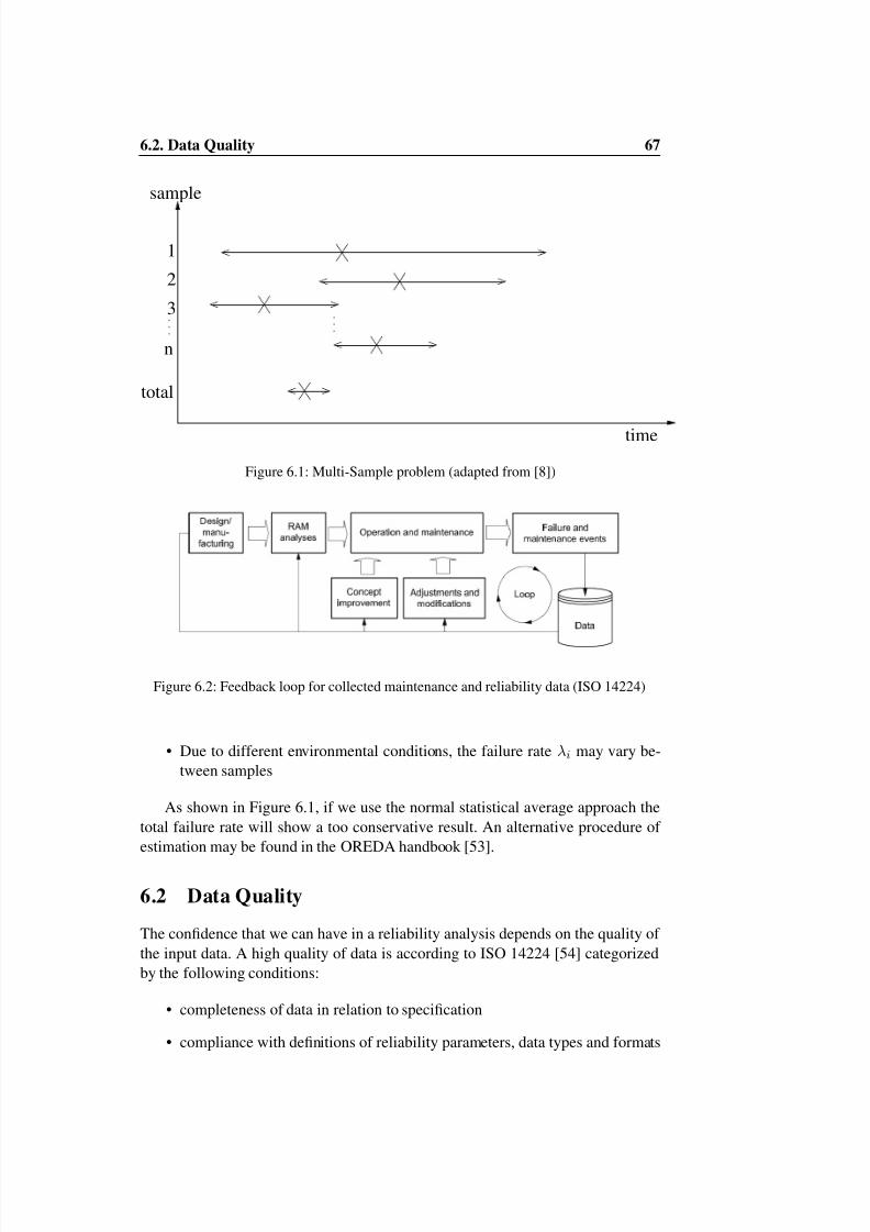
8/6/2019 Gearbox+ +Rossir24 0017
http://slidepdf.com/reader/full/gearbox-rossir24-0017 76/91
6.2. Data Quality 67
1
3
2
n
total
sample
time
Figure 6.1: Multi-Sample problem (adapted from [8])
Figure 6.2: Feedback loop for collected maintenance and reliability data (ISO 14224)
• Due to different environmental conditions, the failure rateλ i may vary be-tween samples
As shown in Figure 6.1, if we use the normal statistical average approach thetotal failure rate will show a too conservative result. An alternative procedure of estimation may be found in the OREDA handbook [53].
6.2 Data Quality
The condence that we can have in a reliability analysis depends on the quality of the input data. A high quality of data is according to ISO 14224 [54] categorizedby the following conditions:
• completeness of data in relation to specication
• compliance with denitions of reliability parameters, data types and formats

8/6/2019 Gearbox+ +Rossir24 0017
http://slidepdf.com/reader/full/gearbox-rossir24-0017 77/91
68 Chapter 6. Routines for Data Collection
• sufcient population and adequate surveillance period to give statistical con-
dence• relevance to the data user needs
It is important that failure reporting cover all failures that occur and the reportsshould contain all relevant information regarding the failure. The quality of col-lected failure data may be inuenced by the following factors. Naturally the mostimportant is the inuence on the equipment itself wich may leas to wrong estima-tion of the equipment reliability. However particular attention should be paid alsoto the the rate of coverage (i.e., have all failures been reported?) and related hiddenfailures.
6.3 Boundaries of Equipment
The boundaries of equipment dene what items are parts of that equipment and thuswhat reliability data shall be collected.It is thus important that the boundaries forequipment data are well dened. If the boundaries of the equipment are unclear itwill be impossible to merge and analyse reliability data from different installations.Theboundary of equipmentmaybe given by text format, gures, drawings etc. TheISO 14224 species boundaries that can be applied for different equipment typesin the process industry.
6.4 Taxonomy
In addition to the boundary description the database should also contain taxonomyfor all equipment.ISO-14224 gives the following denition of the taxonomy:“Thetaxonomy is a systematic classication of items into generic groups based on fac-tors possibly common to a several of the items” . The taxonomy should thus containinformation of all the conditions that may contribute to the reliability characteris-tics of the equipment. It is often common to divide taxonomy into two parts withthe following subdivision:
1. The information regarding the use and the location of the equipment:
a. Industryb. Business Categoryc. Installationd. Plant/unite. ection/System
2. The information about the equipment itself:
a. Equipment Unit

8/6/2019 Gearbox+ +Rossir24 0017
http://slidepdf.com/reader/full/gearbox-rossir24-0017 78/91
6.4. Taxonomy 69
b. Subunitc. Component/Maintainable Itemd. Part
The use/location of the taxonomy needs to be included if data are comparedacross different industries and different installations because environmental andoperational differences may have a large impact on the failure rates of equipment.However, the attention being paid to the rst part of the taxonomy in differentindustries will vary a lot. The main taxonomy for a data source like OREDA ishidden
If the reliability data is to be used for equipment where the assumption of a
constant failure rate is to be applied then it is important that the collection of dataonly starts after the burn-in period. The length of the collecting period will bedependent on the characteristics of the equipment. If the equipment is of highimportance and it is considered to experience few failures over its life time thenthe data collecting period should stretch over a longer time frame than for datawith more failures and of less importance.
The calculation of equipment failure rate is normally based on the operatingtime of the equipment so it is important to gather operating data as well as failuredata. It is important to remember that operating time differs from calendar time asthe equipment may be subject to non-operating periods.
For reliability studies ISO-14224 suggests the collection of the following data:
Equipment unit data:
• classication data; industry; plant, location, system
• equipment attributes; manufacturer’s data; design characteristics etc.
• operation data; operating mode, environment
Maintenance data:
• identication data, e.g. maintenance record number; related failure and
• maintenance data; parameters characterising maintenance, e.g. date of main-tenance, etc.
• maintenance resources; maintenance man-hours; utility equipment/resourcesutilized; etc.
• maintenance times; active maintenance time, down time
Failure data:
• identication data; failures number and related equipment that has failed

8/6/2019 Gearbox+ +Rossir24 0017
http://slidepdf.com/reader/full/gearbox-rossir24-0017 79/91
70 Chapter 6. Routines for Data Collection
• failure data for characterising a failure, failure date, items failed, failure im-
pact, failure mode, failure cause, failure detection method etc.If data are to be compared across different installations it is important that the
reporting is undertaken in a similar manner and preferably on a standard reportsheet. ISO 14224 suggests possible sheets for equipment data (see ISO 14224-Appendix D), for maintenance data and for reporting of failure data (see AppendixE). A uniform denition of failure and a unique method of classication is essentialwhen combining data from different sources into one common database.

8/6/2019 Gearbox+ +Rossir24 0017
http://slidepdf.com/reader/full/gearbox-rossir24-0017 80/91
Chapter 7
Closure
7.1 Conclusions
The wind turbine gearbox is the most critical component in terms of high failurerates and long time to repair. These failures typically cause the entire replacementof the component which it can be extremely costly especially in offshore farmswhere accessibility is reduced. In this thesis it has been shown, how CMS couldbe used for the porpose of maintenance planning and what type of models are themost suitable. An important nding in the present work is that failures in gearboxesare not related to any manufacturing or quality issues and there is not a particulargearbox’s conguration which would result more critical than others.
Condition monitoring is preferredwhere it is not possible to predict trends throughperiodic inspections with accuracy, given that the associated costs are not pro-hibitive; also, where off-line inspections are not desirable (i.e., the inspection re-quires turbine’s shutdown) and where the criticality of a failure justies keepingconstant vigil on the component. In fact, if the costs are not excessive, conditionmonitoring may be more economical than maintenance based on regular inspec-tions.
It has been discussed how one of the challenges of power industry today is toimprove reliability of wind turbine gearboxes. The main reason for the scarce re-liability is the lack of knowledge about the causes of failures which increases theinherent design deciencies. It has also been discussed how, although gearboxeshave been in use for several decades in diverse industries, it is not really possibleto compare a wind turbine gearbox with gearboxes employed in other applicationsfor the reason that a wind turbine gearbox is characterized by stochastic loads dueto the large wind speed variability. Experience from other industry in CBM cannotbe easily applied because of too variable and unpredictable load condition in windturbines. However, it is important to recall that RCM does not increase inherent re-liability. The only way to increase it is by redesign or modication of the design. In
71
8/6/2019 Gearbox+ +Rossir24 0017
http://slidepdf.com/reader/full/gearbox-rossir24-0017 81/91
72 Chapter 7. Closure
this sense, it has been suggested that the real added value of condition monitoring
system should be the components supplier rather than the utility companies.
In the wind power industry CMS are used with the main aim of detecting failuresbefore their occurence. It was shown as the proportional hazards model is a exiblemodel that can be employed for the purpose of maintenance optimization. CMSdata are by nature dened as covariates.
7.2 Future work
The main problem connected to the use of proportional hazards model arises by the
difculties of modeling the covariates due to the stochastic load behaviour of windturbines. Markov chains adopted in this work for modeling covariate dynamiccarries some disadvantage, mainly that we can not assume trends in the changeamong different states. Different types of degradation models for predicting thedynamics of covariates could be used, such as semi-markov processes where thelimitation of exponential transition rates may be relaxed.
When reliability analysis are carried out the estimation of reliability data (mainlyfailure rates) represents a crucial step. It is therefore important to be able to recog-nise all possible failure modes which bring a component to failure. When it comesto wind power industry, and to the gearbox in particular, there are many failures
modes and related causes which have not been yet completely understood.
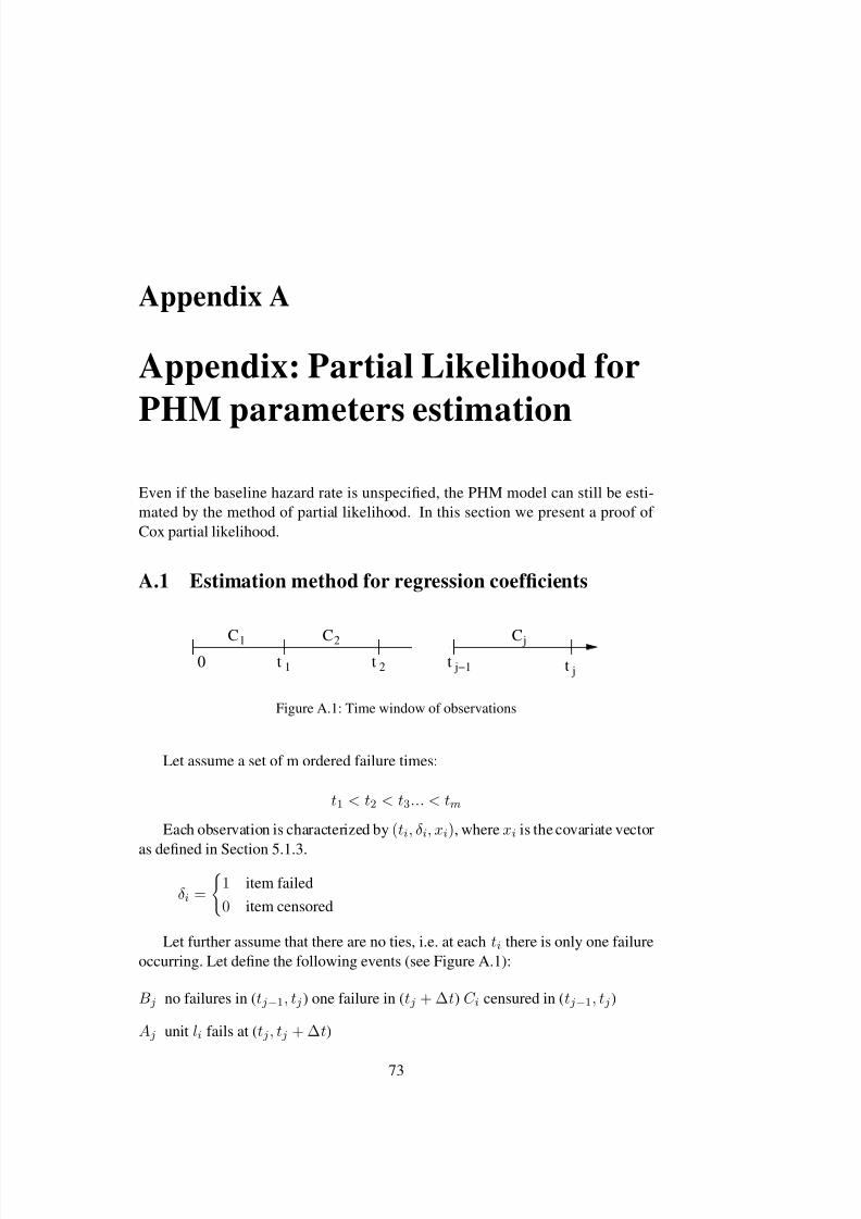
8/6/2019 Gearbox+ +Rossir24 0017
http://slidepdf.com/reader/full/gearbox-rossir24-0017 82/91
Appendix A
Appendix: Partial Likelihood for
PHM parameters estimationEven if the baseline hazard rate is unspecied, the PHM model can still be esti-mated by the method of partial likelihood. In this section we present a proof of Cox partial likelihood.
A.1 Estimation method for regression coefcients
jtt 1
1C 2C jCt 2 j−1t0
Figure A.1: Time window of observations
Let assume a set of m ordered failure times:
t1 < t 2 < t 3... < t m
Each observation is characterized by(t i , δi , x i ), wherex i is thecovariate vector
as dened in Section 5.1.3.
δi =1 item failed0 item censored
Let further assume that there are no ties, i.e. at eacht i there is only one failureoccurring. Let dene the following events (see Figure A.1):
B j no failures in (t j − 1, t j ) one failure in (t j + ∆ t) C i censured in (t j − 1, t j )
A j unit li fails at (t j , t j + ∆ t)
73
8/6/2019 Gearbox+ +Rossir24 0017
http://slidepdf.com/reader/full/gearbox-rossir24-0017 83/91
74Chapter A. Appendix: Partial Likelihood for PHM parameters estimation
C j , C j ⊆∈(1, 2, . . . ,n ) items censured in the interval (t j − 1, t j )
R i Number of items at risk before timet j
The maximum likelyhood method is one of the most common methods in sta-tistical inference. The likelihood function can be dened as the probability of whatit is observed (i.e., failures or censorings) conditioned on the distribution’s param-eters:
P (what we observe| β ) ↔ Likelihood ↔
P (A1 ∩ B 1 ∩ A2 ∩ B 2 ∩ ... ∩ Am ∩ B m )
Given three random events X, Y and Z, from Bayes theorem it follows:
P (X ∩ Y ∩ Z ) = P (X ) · P (Z | Y ) · P (Z | X ∩ Y )
We can now write
P (B 1) · P (A1 | B 1) × P (A3 | A1 ∩ A2) · ...
Let further dene for semplicity
B ( j ) = B 1 ∪B 2 ∪ ... ∪B j
A ( j ) = A1 ∩ A2 ∩ ... ∩ A j
... · P (B 3 | A (2) ∩ B (2) ) × P (A3 | A (2) ∩ B (3) ) × ...
× P (B j | B ( j − 1) ∩ A ( j − 1) )P (A j | B ( j − 1) ∩ A ( j − 1) )
We can now dene
P (B j | B ( j − 1) ∩ A ( j − 1) )
which is the conditional probability of experiencing no failures in(t j − 1, t j ),one failure att j andC j censored given the failures history up to timet j . Censoredevents occur at any time within two consecutives failure times but we have noinformation on the exact time of censoring.It can be showed that the inference of β is only depending on the rank statistics of failure times (see [47], p. 72 for formalproof).

8/6/2019 Gearbox+ +Rossir24 0017
http://slidepdf.com/reader/full/gearbox-rossir24-0017 84/91
A.2. Estimation method for the baseline hazard function 75
The conditional probability of experiencing one failure att j given the failures
history up to before timet j is instead given:
P (A j | B ( j − 1) ∩ A ( j − 1) )
and, for this reason, is dened partial maximum likelihood. From Bayes, wecan rewrite:
P (A | B ∩ C ) =P (A ∩ B | C )
P (B | C )=
=P (li fails | R j are at risk)One fails| R j are at risk) =
z(t ; x lj ) · ∆
r∈Rj
z (t ; x r ) · ∆
where the i-th item failing at timet i is identied by the labelli . The likelihoodfunction is nally obtained by:
L (β ) =m
i=1P (A j | B ( j − 1) | A ( j − 1) ) =
m
i=1
eβ T x l j
r∈R jeβ T x l j
(A.1)
The maximum partial likelihood estimatorβ is the value of β that maximizesL (β ). In practice, it is often easier to maximize the likelihood function log(L (β )) .It is a valid procedure because the logarithm function is monotonically increasing.The estimator of β are then computed by solve the set of equations:
β =
∂logL (β )∂β 1
= 0∂logL (β )
∂β 2= 0
...∂logL (β )
∂β n= 0
A.2 Estimation method for the baseline hazard function
Inferenceβ is independent on the knowledge of the baseline hazard functionz0(t ).The PHM is also known as a semi-parametric method because in the original Coxpaper the baseline hazard rate was considered unknown. In this section a nonparametric estimation method is presented:
Let T 1 < T 2 < T 3. . . < T m be the ordered observed failure times, and letfurther assume that all the censoring times occur at the beginning of the time inter-val [T i− 1, T i ]. It follows that the corresponding cumulative hazard rateZ 0(T 1) <Z 0(T 2) < Z 0(T 3)... < Z 0(T m ) is also orderded.

8/6/2019 Gearbox+ +Rossir24 0017
http://slidepdf.com/reader/full/gearbox-rossir24-0017 85/91
76Chapter A. Appendix: Partial Likelihood for PHM parameters estimation
T T T T1 2 3
All censorings at the beginning of interval
2RR1
n
Figure A.2: Assumptions for obtaining baseline function estimation
Let dene T random variable with cumulative density function F(t). It canbe shown (see [8] , p. 481) that the cumulative hazard rate of any distributioncontinously increasing in time, the following holds:
Z (T ) = − log (1 − F (T )) ∼ exp (1)
The cumulative hazard rate is approximated with and exponential distributionwithλ = 1 . Thus the observed values should lie on a straight line. For the Coxmodel:
Z (T i , x i) ∼ exp (1)
Let deneV i = Z (T i , x i ) = Z 0(T i)e(β T x i )
Z 0(T i) =V i
exp (β T x i)∼ exp (eβ T x i )
Censored times are not giving any information about the failure rate of theunderlined distribution. We introduce the assumption that all censored items occurat the beginning of the interval as shown in Figure A.2. all set riskR i is that willeventually fail after timet i .
Z 0(T 1) = min {Z 0(T i ) for T i ∈R 1} ∼ exp {r∈R 1
eβ T x r }
A well known theorem in reliability sytem theory (see [8]), it states that, givenn independent exponential random variables:
x i ∼ exp (λ i ) → min (x1, x 2,...,x n ) ∼ exp ( λ i )
E (Z 0(T 1)) =1
r∈R 1 eβ T x r
By recalling the memoryless property of the exponential distribution:
Z 0(T 2) − Z 0(T 1) = min {of exp (β T x r ) for r ∈R 2}

8/6/2019 Gearbox+ +Rossir24 0017
http://slidepdf.com/reader/full/gearbox-rossir24-0017 86/91
A.2. Estimation method for the baseline hazard function 77
E (Z 0(T 2) − Z 0(T 1)) = 1r∈R 2 eβ T x r
The number of failures in one interval is assumed to be indipendent from thehistory before the time interval under consideration.
E (Z 0(T 2)) = E (Z 0(T 2) − Z 0(T 1)) − E (Z (T 1)) =1
r∈R 1 eβ T x r−
1
r∈R 2 eβ T x r
In general
E (Z (T i)) =
i
j =1
1
r∈R 1 e(β T x r )
The expected value of Z is a natural estimatorZ . It follows:
Z 0(t ) =t i ≤ t
1
r∈R ieβ T x r
(A.2)
The estimated curve will be a step function. If necessary, baseline distribution’sparameters may be found and approximated by tting a curve to the step function.It can be observed that when the covariates assume null values (i.e.,x i = 0 , no ef-fect on components lifetimes), equation A.2 results in the Nelson-Aalen estimator,
Z 0(t) =t i ≤ t
1R i
which is a very common estimator in non-parametric survival analysis. Detailson the Nelson-Aalan estimator are found in [49] .

8/6/2019 Gearbox+ +Rossir24 0017
http://slidepdf.com/reader/full/gearbox-rossir24-0017 87/91

8/6/2019 Gearbox+ +Rossir24 0017
http://slidepdf.com/reader/full/gearbox-rossir24-0017 88/91
References
[1] J. Moubray.Reliability-Centered Maintenance . 1991. ISBN-10.0750602309.
[2] J. Ribrant. Reliability performance and maintenance - a survey of failures inwind power systems. Master’s thesis, School of Electrical Engineering, KTH,April 2006.
[3] C.A. Walford. Wind turbine reliability: Understanding and minimizing windturbine operation and maintenance costs. Technical report, March 2006.
[4] E. Becker and Paul Poste. Keeping the blades turning: Condition monitoringof wind turbine gears.Refocus, 7(2):26–32, 2006.
[5] K. Rohrig B. Hahn, M. Durstewitz. Reliability of wind turbines experiencesof 15 years with 1500 wts. Technical report, 2005.
[6] L. Rademakers and H. Braam. Assessment and optimisation of operation andmaintenance of offshore wind turbines. Technical report.
[7] Julia Nilsson and Lina Bertling. Maintenance management of wind powersystems using condition monitoring systems - life cycle cost analysis for twocase studies. IEEE Transactions on Energy Conversion , 22(1):223 – 229,2007.
[8] M. Rausand and A. A. Hoyland.System reliability theory: Models and statis-tic methods . John Wiley and Sons Inc., 2 edition, January 2004. ISBN 0-471-47133-X.
[9] L. Bertling.Reliability Centred Maintenance for Electric Power DistributionSystems. Doctoral dissertation, Department of Electrical Engineering, KTH,Stockholm, Sweden, August 2002. ISBN 91-7283-345-9.
[10] J. Cammpbell and A.K. Jardine.Maintenance Excellence . Marcel DekkerInc., New york, USA, 2001. ISBN 0-8247-0497-5.
[11] A.K. Jardine, D. Lin, and D. Banjevic. A review on machinery diagnosticsand prognostics implementing condition-based maintenance. Technical re-port, 2005. CBM Lab, Department of Mechanical and Industrial Engineering,University of Toronto.
79
8/6/2019 Gearbox+ +Rossir24 0017
http://slidepdf.com/reader/full/gearbox-rossir24-0017 89/91
80 REFERENCES
[12] Albert H.C. Tsang. Condition-based maintenance:tools and decision making.The Hong Kong Polytechnic University, Hong Kong , 1995.
[13] J. Hoin. Interview.SPM Instrument AB Sweden , March 2007.
[14] S. Dekker. Applications of maintenance optimization models: a review andanalysis.Erasmus University, Rotterdam, The Netherlands , 1996.
[15] R. Allan, G. Anders, and R. Billinton. The present status of maintenancestrategies and the impact of maintenance on reliability. Technical report,2001. IEEE Transactions on Power systems.
[16] A. Wilson.Asset Maintenance Management . Industrial Press Inc., 2 edition,2002. ISBN 0-8311-3153-5.
[17] A. Jardine and Tsang H.T.C.Maintenance,Replacement and Reliability . Tay-lor & Francis, Boka Raton, Florida, august 2006. ISBN 0-8493-3966-9.
[18] J. Vatn. World class maintenance. Technical report, 2006. NTNU, mainte-nance optimization course compendium.
[19] T.M. Welte, J. Vatn, and J. Heggest. Markov state model for optimization of maintenance and renewal of hydro power components.Probabilistic Methods Applied to Power Systems, 2006. PMAPS 2006. International Conference on ,pages 1–7, 11-15 June 2006.
[20] IEC 60812, Analysis techniques for system reliability and effects analysis(FMEA) . 2nd edition, January 2006.
[21] Military Standard 1629A, Procedures for performing Failure Mode, Effectsand Criticality Analysis . November 1980. Department of Defense, USA.
[22] Mario Villacourt. Failure mode and effects analysis (fmea): A guide for con-tinuous improvement for the semiconductor equipment industry. Technicalreport, 1997. SEMATECH, Technology Transfer.
[23] M. Beuregard R. Mcdermott, R. Mikulak.The Basics of FMEA . ResourceEngineering Inc., 1996. ISBN 0-527-76320-9.
[24] J. Peeters.Simulation of dynamic drive train loads in a wind turbine . PhDthesis, Katholieke Universiteit Leuven, Leuven, Belgium, June 2006. ISBN90-5682-728-6.
[25] S. Derek. Gear Noise and Vibration . Marcel Dekker, Inc., New York, 2edition, 2003. ISBN 0-8247-4129-3.
[26] H. Stiesdal. The wind turbine components and operation. Autumn 1999.

8/6/2019 Gearbox+ +Rossir24 0017
http://slidepdf.com/reader/full/gearbox-rossir24-0017 90/91
REFERENCES 81
[27] J. Manwell, J. McGowan, and L. Rogers.Wind Energy Explained, Theory,
Design and Application . John Wiley and Sons Inc., 2 edition, 2002. ISBN0-471-49972-2.
[28] T. Burton.Wind energy :Handbook . J. Wiley, New York, 2001. ISBN 1-59124-747-0.
[29] J. Muller. The lubrication of wind turbine gearboxes. Technical report, May1993.
[30] J. Losl and O. Holstein. Aligning drive trains in wind power plants. 2003.
[31] L. Rademakers P. Eecen, H. Braam. Development of operations and mainte-
nance cost estimator. Technical report, March 2006.[32] Advanced maintenance and repair of operation and maintenance of offshore
wind farms using fault prediction and condition monitoring technique. Tech-nical report.
[33] E.Von Renouard.Wind Turbines . Springer Berlin Heidelberg, 2005. ISBN978-3-540-24240-6.
[34] J. Cohen. A methodology for computing wind turbine cost of electricity us-ing utility economic assumptions. Technical report, 1989. Windpower 89Proceedings.
[35] H. Higgins.Maintenance Engineering Handbook . McGraw-Hill Inc., 5 edi-tion, 1995. ISBN 0-07-028811-9.
[36] Sven-erik thor, vattenfall ab.
[37] K. Holmberg. Tribological bases for accellerated testing. Technical report,May 1990.
[38] J.Muller R. L. Errichello. How to analyze gear failures.Geartech , January2001.
[39] Requirements for condition monitoring systems, allianz zentrum fur technikgmbh. Technical report, 2002.
[40] K. Keith Mobley.An introduction to Predictive Maintenance . 2002. ISBN0-7506-7531-4.
[41] H. Braam T. Verbruggen. Generic failure modes relevant for condition mon-itoring. Technical report, April 2004.
[42] SPM Instruments AB. Condition monitoring solutions for windfardms.SlidesPresentation , January 2007.
8/6/2019 Gearbox+ +Rossir24 0017
http://slidepdf.com/reader/full/gearbox-rossir24-0017 91/91
82 REFERENCES
[43] J. Caselits, J. Giebhardt. Advanced maintenance and repair for offshore wind
farm using fault prediction techniques. Technical report, 2004. ISET.[44] A. Holmberg, K. Folkeson.Operational Reliability and Systematic Mainte-
nance . Elsevier Science Publishing Co.Inc, 1991. ISBN 1-85166-612-5.
[45] N. Tandon and A. Parey. Condition monitoring of rotatory machines. Tech-nical report, 2002.
[46] J. Smith. Development of a generic wind farm scada systemm. Technicalreport, 1993.
[47] J. Kalbeisch and R. Prentice.The statistical analysis of failure time data .
New York : Wiley, 1980.[48] D.R. Cox. Regression models and life tables.J. of Royal Statistical Society ,
B34:187–220, 1972.
[49] J. Ansell and M. Phillips.Practical methods for reliability data analysis . SN0-19-853664. Clarendon Press, 1994.
[50] A.K.S Makis V., Jardine. Optimal replacement in the proportional hazardsmodel.INFOR , 1992.
[51] CBM Lab. Exakt software for optimizing cbm. OMDEC.
[52] E. Lee and J. Wang.Statistical Methods for Survival Data Analysis . WileySeries in Probability and Mathematical Statistics. Hoboken, N.J. John Wiley& Sons, Inc. (US), 2003.
[53] SINTEF Industrial Managament, editor.Offshore Reliability Data . OREDAPartecipants, 4th edition edition, 2002.
[54] Iso-14224 petroleum, petrochemical and natural gas industries – collectionand exchange of reliability and maintenance data for equipment. Technicalreport, ISO International Standards for Organizations, 2006.