UPTEC F 18031

Examensarbete 30 hpJuni 2018

Gimbal stabilizer for cockpit bases of terrain vehicle or combat boat A proof of concept

Joel Larsson

Teknisk- naturvetenskaplig fakultet UTH-enheten Besöksadress: Ångströmlaboratoriet Lägerhyddsvägen 1 Hus 4, Plan 0 Postadress: Box 536 751 21 Uppsala Telefon: 018 – 471 30 03 Telefax: 018 – 471 30 00 Hemsida: http://www.teknat.uu.se/student

Abstract

Gimbal stabilizer for cockpit bases of terrain vehicle orcombat boat

Joel Larsson

The purpose of this project was to construct a 2-axis stabilized model platform, as a proof of concept, intended to use for a cockpit base of a terrain vehicle or a combat boat. The stabilization of the platform in the roll and pitch axes is realized using a feedback control system that contains a proportional-integral-derivative (PID) controller, two DC motors driving the roll and pitch movements, and a 6-axis inertial measurement unit (IMU) measuring the roll and pitch angles.The project started with a study of various stabilized platforms and the theories behind them and a model of the system was created in SimuLink to simulate the system and design the controller. After the simulations where satisfactory a model platform of a scaled-down actual size was constructed. The platform’s frame was printed in a 3D printer. The control system for the platform has been implemented. The PID controller was implemented on the Arduino Mega 2560 development board, and it regulates the pitch and roll movements through two DC motors. The platform’s pitch and roll angles are measured by a 3-axis gyroscope in an IMU sensor (MPU-6050). The measurements are processed by a Kalman filter implemented on the Arduino board to reduce the noise.The Simulink simulation provided a functioning control system. However, the prototype of the implemented model platform does not work with god stability as expected. The reason for this result is mostly due to the unsuccessful construction of the platform frame and the bad choice of motors.

ISSN: 1401-5757, UPTEC F 18031Examinator: Tomas NybergÄmnesgranskare: Ping WuHandledare: Rasmus Muhrbeck

ii

Populärvetenskaplig sammanfattning

När man kör ett terrängfordon eller en stridsbåt i antingen väldigt kuperad terräng eller i stormigt vatten så är det lätt att tappa orienteringen eller bli åksjuk. Om man kan stabilisera cockpiten till ett sådant fordon så att den håller sig mer horisontell kan man minska dessa negativa effekter av att färdas med ett sådant fordon. För att kunna skapa en sådan stabilisering kan man använda sig av reglerteknik.

Idag ser vi ofta hur reglerteknik används i samhället för att underlätta för oss, ett sådant exempel är styrservot i bilen, som underlättar styrningen och kontrollen av bilen. Även farthållaren är ett reglersystem. Ett reglersystem är ett system som med hjälp av återkoppling försöker påverka en utsignal att följa ett önskat värde som bestäms av en användare. I exemplet med styrservot så sätts det önskade värdet av användaren genom att vrida på ratten och system korrigerar bilens däck tills det att däckens position matchar det som föraren visar med sin ratt.

Ett sådant reglersystem skulle kunna användas för att kontrollera en plattform och hålla den horisontell, för att sedan använda den plattformen som bas för en cockpit. Här är vinkelutslaget på plattformen det man vill styra och det önskade värdet skulle då vara noll grader mot horisonten, dvs att plattformen ska hållas horisontell. Syftet med detta projekt är att undersöka teorin bakom liknande stabiliseringskonstruktioner, även kallade gimbals, och försöka konstruera en demonstratör för att visa på att en sådan konstruktion är möjlig.

För att kunna styra ett reglersystem behöver man kunna mäta utsignalen, däckens vridning eller bilens hastighet eller plattformens position, för att systemet ska kunna regleras, någon typ av sensor. I det här projektet har en tröghetssensor använts, även kallat IMU. Denna IMU består av tre accelerometrar, som mäter accelerationen som sensorn utsätts för i tre dimensioner, och tre gyroskop som mäter sensorns rotationshastighet i tre dimensioner. Dessa kan kombineras för att skapa en bild av sensorns rotation och genom att placera IMUn på plattformen man vill kontrollera så kan man mäta plattformens rotation, vilket är det man vill reglera.

Innan en demonstratör kan konstrueras bör man skapa en modell av systemet och göra relevanta simuleringar för att se hur systemet kommer kunna reagera och för att se vilken typ av regulator som kan behövas. Simuleringarna i denna rapport har gjorts i ett program som heter SimuLink och för att utvärdera olika regulatorer så kan ett stegsvar användas. När simuleringarna givit tillfredställande resultat så kan demonströren designas och konstrueras. Den mekaniska delen av konstruktionen bestod av en 3D printad ram och plattform och två DC motorer som styrde rotationen av plattformen. Dessa motorer var kopplade via en H-brygga till en Arduino som innehöll mjukvaran. Mjukvaran bestod av avläsning och behandling av datan som IMUn gav systemet. För att kunna använda de värden som lästes av krävdes att ett Kalmanfilter implementerades för att reducera bruset. Två PID regulatorer implementerades också för att reglera systemet.

Simuleringarna som gjordes i projektet visar att det är möjligt att skapa ett reglersystem för en sådan konstruktion, men att det var svårt att realisera systemet i praktiken. I slutändan visade det sig att större vikt borde ha lagts på valet av motorer samt att designen och konstruktionen av demonstratören kunde ha förbättrats.

iii

Contents Abstract ...................................................................................................................................... i

Populärvetenskaplig sammanfattning .................................................................................... ii

Contents .................................................................................................................................... iii

1 Introduction ...................................................................................................................... 1

1.1 Background ............................................................................................................................. 1

1.2 Purpose and goals .................................................................................................................... 1

1.3 Specifications and scope.......................................................................................................... 1

1.4 Tasks and methods .................................................................................................................. 2

1.5 Outline ..................................................................................................................................... 2

2 Theory ............................................................................................................................... 2

2.1 Control theory .......................................................................................................................... 2

2.2 DC motors ............................................................................................................................... 4

2.3 Platform ................................................................................................................................... 7

2.4 Inertial measurement unit ........................................................................................................ 9

2.5 Kalman filter .......................................................................................................................... 10

3 Implementation ............................................................................................................... 11

3.1 System overview ................................................................................................................... 11

3.2 Hardware and components .................................................................................................... 12

3.3 Measurements ........................................................................................................................ 15

3.4 Matlab and SimuLink ............................................................................................................ 18

3.5 Integrated Development Environment .................................................................................. 20

3.6 Development tools ................................................................................................................. 20

3.7 Mechanics .............................................................................................................................. 21

3.8 Regulator ............................................................................................................................... 23

4 Results and discussions .................................................................................................. 23

4.1 Calculations ........................................................................................................................... 23

4.2 Mechanics .............................................................................................................................. 27

4.3 Software................................................................................................................................. 29

5 Conclusions and future work ........................................................................................ 34

5.1 System identification/Simulations ......................................................................................... 34

5.2 Regulator ............................................................................................................................... 34

5.3 Mechanics .............................................................................................................................. 35

5.4 Complete system ................................................................................................................... 35

References ............................................................................................................................... 36

iv

Appendices .............................................................................................................................. 38

A. Full derivation for DC motor transfer function ............................................................................ 38

B. Proof that KT equals KE in SI-units ............................................................................................... 39

1

1 Introduction

1.1 Background

When a terrain vehicle travels through rough terrain at high speeds or when a combat boat

rides through rough waters, the vehicle will shake a lot, which results in a hard time for the

persons driving the cockpit. To counter the severe disturbance in such rough environment and

facilitate driving, it is needed to stabilize the cockpit. By doing this the persons controlling the

vehicle will be less susceptible to motion sickness or disorientation. An effective solution to

this problem is to use a gimbal stabilizer.

A gimbal is a frame or support that can pivot around one axis and thus lets an object attached

to it rotate in one axis as well. To get more than one degree of freedom more than one gimbal

is used. The gimbal has been known as a theory for a long time and the first description of it

dates back to around 280BC, by a Greek inventor. There are also some mentions of gimbals in

ancient Chinese history as well, and in around 180BC a Chinese inventor created a gimbal

incense burner. Later in history the gimbal and combination of gimbals have been used for

many purposes for example stabilizing compasses on ships, so that even if the ship rocks due

to waves, the compass is horizontal [1].

Inertially stabilized platforms (ISP) often make use of gimbals in order to stabilize a platform

on which some sort of payload can be mounted. ISPs are used in many applications, for

example the compass construction mentioned above is a form of ISP and today they are used

in camera stabilizers for aircrafts or sensors attached to moving vehicles. They are used to

control the line of sight of an object in relation to another object. In these types of applications

some type of automatic control is often used. By using feedback from the platform and a

regulator, for example a proportional-integral-derivative (PID) controller, the platforms

rotation can be controlled if coupled with some kind of motors driving the platforms rotation

[2].

1.2 Purpose and goals

The purpose of this project is to create an inertially stabilized platform as a proof of concept

for a cockpit base for a terrain vehicle. Ideally a cockpit base would be constructed. But

because of the size of the project this was not an option, instead the main focus of this project

is to create a scaled-down demo construction.

1.3 Specifications and scope

For the ISP to be created, we want to control the line of sight of a cockpit in relation to the

vehicle it is attached to. The cockpit needs to be controlled in two degrees of freedom, roll

and pitch, to be able to stabilize by countering the roll and pitch motion of e.g. a boat in rough

waters.

To this purpose, a feedback control system needs to be built that consists of a PID-controller

on an MCU, two DC motors controlled by the PID to regulate the pitch and roll movements of

the platform, and an inertial measurement unit (IMU) consisting of a 3-axis accelerometer and

a 3-axis gyroscope that measures the pitch and roll angles of the platform. The measurements

2

of the gyroscope are processed by a Kalman filter to calculate the pitch and roll angles of the

platform.

Due to restrictions in time, this project is only focused on constructing a model of the

stabilized platform with a scaled-down size, simply called model platform or prototype in the

rest of the report, intended for a proof of concept.

1.4 Tasks and methods

To achieve the above-mentioned goals with consideration of the specifications, the project is

conducted with the following tasks:

Literature study

Designing of the control system

Simulations of the control system

Construction of the framework for the stabilizing platform

Implementation of the control system

Testing and evaluation of the implemented system

In the startup phase of the project a time plan was made for the duration of the project, but

during the course of the project this plan has been revised more than one time.

The literature study presented most of the theory behind the designing of the finished system

and restrictions on the control system. It also provided information on which type of sensors

should be used and how they could be implemented. The construction was designed in the

program SolidWorks and then 3D-printed.

The system was then designed in Matlab and SimuLink. For this, certain parameters of the

motors were needed and therefore some experiments had to be done. During the design of the

control system, simulations in SimuLink were done to see how the system would react to

disturbances.

1.5 Outline

In the following chapters of the report the theory behind the project will be presented, starting

with control theory, which is essential to an ISP, followed by DC motor theory, the mechanics

behind the stable platform, and theory of how an IMU sensor can be implemented in software.

Then the implementation of the theory will be presented, with subchapter on the hardware,

simulations that have been done, the software implementation and how the ISP was

constructed. Then the results will be presented and discussed followed by a conclusion and

recommended future work.

2 Theory

2.1 Control theory

Feedback control system

To control the system a regulator is implemented with the use of feedback from the IMU. This

regulator then sends a signal to the motors to react to the change in rotation of the platform. In

3

Fig. 2.1 one can see how such a system can be represented, with this project’s different

blocks. The controller will be a PID, the actuator is the H-bridge and the motors, the process

is the platform with its roll and pitch angles as controlled variables, and the sensor is the IMU.

Fig. 2.1 Block diagram of a feedback system

PID controller

The PID controller is one of the commonly used regulators in the world. This is mostly

because of its rather simple algorithm and the fact that it can be used in so many applications

as long as the process has a measurable output, an ideal value for the output and an input to

the process [3]. The complete PID is expressed as

�(�) = ��ε(t) + �� ∫ �(�)���

�+ ��

��(�)

�� (2.1)

Where �(�) is the control signal, �(�) is the error, and ��, �� and �� are constants providing

weights on the proportional, integral and derivative terms respectively. These three constants

are called the tuning parameters and by changing their values, the controller will behave

differentially. The error, �, is the result of comparing the measured output to the desired

output. These three terms working together on the error tend to make this error be zero. For

example, in the case of this project the actual output is the pitch and roll angles of the

platform measured by the IMU and the desired output is a horizontal angle, which the system

should aim towards.

The output of the proportional part of the controller is the proportional gain multiplied with

the error. In other words, if the error of the system output is large, the control signal will be

large. The good side of this is that it is easy to understand and implement, but it also means

that when the error gets small, so will the control signal. In fact, in theory the control signal

can never erase the error completely and this is called a steady state error. If one wants to

counter this and use a larger proportional gain, the system will in turn be less stable and

overshoot.

To counter the steady state error, or offset, an integral part is added to the control loop. The

integral part reduces the error over time and can therefore erase the steady state error

completely. The integral part changes the control output at a fast rate if the error is large and

at a slower rate if the error is small. With this part the steady state error can be erased, but the

overshoot and oscillations of the control signal will often increase.

4

The derivative part responds to the rate of change of the error. If the error changes at a faster

rate, the derivative part will put out more control signal. If this part of the PID is tuned well,

the proportional and integral parts can be more aggressive, since the overshoot this produces

will be handled by the derivative part. The downside of using the derivative part is that it is

quite sensitive to measurement noise, since these often change very much. The derivative part

however is not always present in process controllers and often a version of the PID controller

is used, called PI controller [4]. The derivative part will for example make the tuning of the

controller more difficult and is therefore skipped in controllers where it is not necessary. In

motion control it is often used though.

The tuning process of the parameters is important to get the wanted response from the system.

When PID controllers were introduced, most of the tuning was done by trial and error, but

nowadays there are several different methods for this and the choice of tuning method

depends on the specifications of the system. There is also software that helps with the tuning,

for example Simulink and Matlab have a built in PID tuner were the user can change the

speed or the transient behavior to desired values and the tuner updates the tuning parameters

accordingly [5].

2.2 DC motors

To control the roll and pitch movements, two DC motors are needed. In a DC-motor electrical

energy is converted to mechanical energy with forces produced by magnetic fields. To design

a controller in MATLAB Simulink, a theoretical model of the motors is needed. Therefore,

the in-depth theoretical study is presented here. An electrical schematic of a DC motor is

shown in Fig. 2.2. One can see that the applied voltage, VIN, equals the voltage drop over the

inductance and resistance and the electromotive force (EMF), which is the voltage produced

by the motor in motion. Mathematically, this can be expressed as

��� = �� + ���

��+ ���� (2.2)

Where VIN is the applied voltage, I is the current, R is the internal resistance of the motor, L is

the internal inductance and VEMF is the voltage produced by the rotation of the motor.

5

Fig. 2.2 Free body diagram of a DC motor where v is the applied voltage, e is the EMF voltage, Tis the produced torque, θ is

the produced angular velocity and b�̇ is the frictional force [6]

This can be related to the mechanical equations of the motor. The armature current is

proportional to the torque of the motor by a constant KT, called the torque constant, which is

written as [7]

� = ��� (2.3)

According to [8] the total torque of the motor is the motor torque TM minus the friction torque

of the motor, TF. The friction torque is a function of the angular velocity and in chapter 2.2.1

different models of friction will be presented. The total torque can then be described as the

total inertia, J, of the rotor and load multiplied with the angular acceleration of the motor.

Mathematically this can be written as

��̈ = ��� − ��(�̇) (2.4)

Similar to how the motor torque could be described by the motor torque constant and the

current, the back-EMF voltage can be related to the angular velocity of the rotor and it is

proportional with a constant Ke, which is the back-EMF constant, which can be written as

���� = ���̇ (2.5)

To be able to model the DC motor and then design a controller, its transfer function is needed

and therefore we want to find how the angular velocity is related to the input voltage, VIN. By

using the Laplace transform and combining the relations described, the transfer function for

the DC motor is found and expressed as

�̇

���=

��

(����)��������̇�������

(2.6)

A detailed derivation of the transfer function, equation (2.6), is given in Appendix A.

6

Friction and how to model it

The friction inside a DC motor can be modelled as a linear function proportional to the

angular velocity with a constant FV, known as the viscous friction. It is often adequate to only

take this part of the friction into consideration when modelling a DC motor. However, to get

closer to the real system and the dynamics of the DC motor one has to look at the other parts

of the friction, often nonlinear. These parts will now be presented.

2.2.1.1 Static friction

The static friction, also called stiction, is the friction force that an external force needs to

overcome to get something moving and is often called the breakaway force. This friction

force, FF, can be described by

�� = �� (2.7)

when the angular velocity is zero and the static friction is larger than the external force, ��.

When the angular velocity is zero but the external force is larger than the static friction force,

��.

�� = �����(��) (2.8)

As we can see by these equations the static friction gives the model a discontinuity in zero,

which can be hard to model.

2.2.1.2 Coulomb friction

The Coulomb friction, FC, also depends on the sign of the velocity, but not the magnitude.

The value of the coulomb friction is often lower than the static friction. The coulomb friction

can be expressed as

�� = �����(�) (2.9)

Where � is the angular velocity, which can also be written as �̇. Since the signum function is

zero at zero angular velocity the friction is also zero here, however as soon as the motor

begins to move, the friction makes a step with the magnitude of ��.

2.2.1.3 Stribeck effect

The Stribeck effect causes the friction to drop with higher velocities until a so called Stribeck

velocity is reached. From this point the friction will take the form of the viscous friction. The

Stribeck effect can be described as

�� = �

��(�), � ≠ 0

�� , � = 0 ��� |�� < ��|

�����(��), ��ℎ������

(2.10)

As we can see, this effect looks similar to the static friction [7].

7

Friction models

To take these effects of friction into account, several models have been developed and used to

describe systems with friction. The simplest models only take into account one of these

effects or just some, these are called steady state models. One of the more complex steady

state models is the Stribeck friction model, which is described by

��(�) = �� + (�� − ��)���

�

����

+ ��� (2.11)

where FF is the friction, �� is the coulomb friction, �� is the static friction, �� is the viscous

friction and �� is the Stribeck angular velocity.

In more recent years dynamic friction models have been developed such as the LuGre model

and GMS model. This report will however not go into details about these models [9].

2.3 Platform

The main focus of this project is to create a scaled-down demo platform. Therefore, the in-

depth theoretical study is presented here. The schematic of the platform is illustrated in Fig.

2.3. In the figure the platform can move around two axes regulated by two DC motors. The

inner motor controls the pitch angle and the outer motor controls the roll angle.

Fig. 2.3 Sketch of platform

8

Inertia

Inertia is an object´s resistance to move from its state of motion. In an ISP there are several

rigid bodies that rotate and therefore have an inertia that needs to be taken into consideration

when controlling the rotation of them. In this project there is the platform and the inner

gimbal that rotates. The torque acting on these bodies come from the DC motors and to know

how much force is needed to rotate the body a certain amount, the inertia is needed.

The system can be seen in Fig. 2.6. Since the axis of rotation can be considered as principal

axis, the angular velocity will be in the same direction as the angular motion, and therefore

the inertia can be calculated as a scalar with direction vector in the direction of the x-axis in

Fig. 2.6 [8]. If the rotational axis is not a principal axis, one needs to calculate the inertia

using so called tensors. For these calculations there are predefined formulas and the one for

the platform can be expressed as [10]

��������� = �

����� (2.12)

For the inner gimbal some approximations have to be made, and the motor has to be taken

into account. Since the motor will have a weight, a counter weight is needed to balance the

mass of the system around the axis. So, to calculate the inertia we assume that the system is a

cuboid with two point masses at the same distance on each side of the axis, which can be

written as

������� =�

���������(�� + ��) (2.13)

������ = 2�������� (2.14)

���� = ������� + ������ (2.15)

With ������� as the mass of the system without the mass of the motor, ������, a as the

length of the cuboid, b as the height of the cuboid and r as the distance from the axis to the

motor.

However, if a payload is added to the platform, the inertia will change and needs to be

recalculated. This is done by adding the inertias together since inertia is additive, which can

be expressed as

���� = ��������� + �������� (2.16)

Torque

Torque can be described as rotational force and the formula for calculating torque can be

written as

� = � × � (2.17)

As we can see torque is a vector and thus have a direction, which will be in the same direction

as the angular momentum. The torque can also be related to the inertia and angular

acceleration, which can be written as

9

� = �� (2.18)

With this relation it is easy to calculate the magnitude of angular acceleration that is possible

to get from a given DC motor given the inertia of the gimbal or platform.

2.4 Inertial measurement unit

To implement the use of the controller in the prototype, a theoretical knowledge of the sensor

is needed. Therefore, the in-depth theoretical study is presented here. An inertial measurement

unit (IMU) is a device that often consists of one or more sensors that together can measure the

movement of the sensor, for example an accelerometer. Depending on the number and types

of sensors an IMU contains it can measure more degrees of freedom. An accelerometer can

measure the acceleration in three directions, which gives the sensor three degrees of freedom.

If a gyroscope is added, which measures the rotational velocity in three directions, the

combination of the sensors gives the IMU six degrees of freedom. These two sensors are the

most common in simple IMUs and can be used to describe an objects rotation in relation to

gravity. There are of course more complex IMUs containing more sensors, for example a

magnetometer, which measures the magnetic field in three directions, that gives the IMU nine

degrees of freedom.

By combining different sensors like this it is possible to get new information from them that

would not be possible with the sensors separated, this is called sensor fusing. For example,

with the combination of an accelerometer and a gyroscope it is possible to calculate the pitch

and roll angle of a platform, which is used in inertially stabilized platforms. To do this a filter

is needed. There are different types of filters that can be used depending on the complexity of

the system, but one of the more common is the Kalman filter [11]. The filter is also used

because the raw data from the sensors are often really noisy which can destabilize the

feedback loop.

The raw values need to be calculated from the data transmitted from the sensor. The data that

the IMU delivers from its sensors are digital values and their range depend on the IMU, for

example the MPU-6050 transfers values of signed 16-bit integers, which means that the value

of the data ranges from -32768 to 32767. To use these values, one need to know the

sensitivity of the sensors and convert the raw data into values that can be used, for example

g’s in case of accelerometer and degrees per second for the gyroscope. In the case of the

MPU-6050, the sensitivity of the accelerometer is ±2g, which means that 1g is equal to the

value 16384. The same method can be applied to the gyroscope. One also needs to calibrate

the sensor to find which values represent the zero-position [12].

By calibrating the sensor, the offsets can be found, this is done by reading the values of the

sensors when the IMU is leveled, doing this several times and then take the mean for each

parameter will give the offset. When the offset and the scale of the values are known, the real

values of the measured data can be calculated. This can be written as

�� =��������������

����� (2.19)

Where the acceleration in x direction are calculated in units of g’s.

10

When the data has been converted into units of g’s and degrees per second, they can be

converted again into degrees, which can be written as [13]

���������� = arctan ����

���� ���

�� (2.20)

��������� = arctan ���

��� (2.21)

The Kalman filter is then applied to these values.

2.5 Kalman filter

The Kalman filter is what is called an observer in control theory. It is used to make a guess of

how a system will behave. A state representation of a system is often important, however the

states themselves are often not observable and only the input and measured output can be

observed. In such an event the states should be estimated or reconstructed. and this is where

the observer comes in. The Kalman filter is such an observer and is even called the optimal

observer [14].

In this application a gyroscope and an accelerometer are used to measure and calculate the

angle of a platform. Both these sensors contain noise that will give the calculated angle an

error. In case off the accelerometer it is very noisy and if the system reacted to this noise the

platform would shake a lot. It does however give a good approximation of the long-term

changes in the acceleration, and by extent the angle of the platform. The gyroscope on the

other hand gives a good short-term approximation of the angle but will with time start to drift.

These two sensors would not be able to give a good approximation by themselves, but with

the Kalman filter they are fused to give the system a good estimation of the platform´s angle.

The algorithm of the Kalman filter can be divided into two groups, the prediction step and the

correction step. The Kalman filter starts by predicting the next state of the system. It then gets

feedback from measurements and corrects the first prediction. These predictions and

corrections only take the previous state into account, which means that the algorithm is often

light on the memory and works well for real time applications such as an inertially stabilized

platform [15].

In the following equations the Kalman filter algorithm will be shown for the pitch [16]. The

state equation for the system can be written as

�� = ����� + ��̇� + �� (2.22)

with x, F and B defined as

�� = ��

�̇�����

�

(2.23)

� = �1 −��0 1

� (2.24)

11

� = ���0

� (2.25)

With � as the angle and �̇���� the drifting in the gyroscope, �̇� as the angular velocity

measured by the gyroscope and dt as the delta time, which is the short time since the last

measurement. The measurement �� is given by

�� = ��� + �� (2.26)

with H defined as

� = [1 0] (2.27)

The algorithm starts with the prediction step, where the current state is estimated based on the

gyroscope measurement and the previous state as follows

���|��� = ������|��� + ��̇� (2.28)

Then the covariance matrix �� is estimated based on the previous covariance matrices, the F

matrix and Q, which is the covariance matrix of the process noise, ��. This can be expressed

as

��|��� = �����|����� + �� (2.29)

Now the prediction step is done and it is time for the correction step where we update the

estimated state based on the estimate and the innovation, ��, and the Kalman gain, ��. The

covariance matrix �� is also updated, which can be written in the following manner

���|� = ���|�� � + ���� (2.30)

��|� = (� − ���)��|��� (2.31)

With ��, �� and �� defined as

�� = �� − ����|��� (2.32)

�� = ��|��������� (2.34)

�� = ����|������ + � (2.35)

R is the covariance for the measurement noise and is not a matrix and not dependent on the

time.

3 Implementation

3.1 System overview In chapter 2.1 a typical feedback control system was shown. How each block where

implemented in this project is shown in Fig. 3.1. In this chapter we will look at the different

12

blocks and see how they work, both separately and together with each other. The system has

been simulated in Matlab and SimuLink before it was implemented on a micro controller.

Fig. 3.1 Block diagram over the feedback system

3.2 Hardware and components

Micro controller

To implement the system the Arduino Mega 2560 board, shown in Fig 3.3, was used and it is

based on the ATmega 2560 micro controller. We decided to use an Arduino board since the

chosen IMU sensor had good libraries for Arduino, which we had some previously knowledge

of working with. This also made the choice of the Mega 2560 since the libraries are rather

large and therefore the controller needed much memory. The Arduino Mega board was

chosen over the Arduino UNO board because of this reason, since the ATmega328p on the

UNO has 32 KB of flash memory and the ATmega2560 on the Mega board has 256 KB of

flash memory. In table 3.1 the specifications of the Arduino Mega is presented [17].

Table 3.1 Specifications for the Arduino Mega

Parameter Value

Operating voltage 5V

Input voltage 7-12V

Digital I/O pins 54 (where 15 provide PWM output)

Analog input pins 16

Flash memory 256 KB

SRAM 8 KB

EEPROM 4 KB

Clock speed 16 MHz

13

IMU

To control the system a sensor is needed in the feedback loop. It gives the controller

information on what the current angle of the platform is and by subtracting this value from the

reference signal, we get an error the controller can correct. In this project an IMU was needed

with a gyroscope and an accelerometer. The Sparkfun MPU-6050 was chosen, shown in Fig.

3.2, which contains a 3-axis gyroscope and a 3-axis accelerometer. For the sensor the GY-52

break out board was used, which has a voltage regulator so that the board can be powered

with either the 3.3V or the 5V. The MPU-6050 was chosen since it fulfilled the requirement

of having both a gyroscope and an accelerometer, but it also has a large library written by Jeff

Rowberg, that makes the use of the sensor much simpler.

Fig. 3.2 The Sprakfun MPU-6050 on a different breakout board than GY-52 [18]

Electronic circuit

To support the system an electronic circuit was needed. The micro controller hade to be

connected to the DC motors and the sensor and the controller and the motors needed power to

function. For the power a LiPo battery with 2 cells was chosen, that could deliver power for

both the motors and the micro controller, it gives out a voltage around 7.4 V and can deliver

up to 132 A. As we can see in table 3.1, 7.4 V is enough to power the microcontroller. The

DC motors need a voltage at around 6 V and therefore a voltage regulator is needed. An H-

bridge was used to control the two motors with PWM signals from the micro controller. It was

decided that the H-bridge and voltage regulator would not be designed and constructed, but

instead bought to save time. In Fig. 3.3 we can see a picture of the assembled circuit, where A

is the Arduino Mega 2560 board, B is the Dual Channel H-bridge and C is the XH-M404

voltage regulator.

14

Fig. 3.3 The assembled electric circuit, where A is the Arduino Meg 2560 board. B is the Dual Channel H-bridge and C is the XH-M404 voltage regulator

DC motors

The DC-motors that were used needed to be fast to be able to respond to the change in the

platforms angles and to react as fast as the controller. To find such a motor the torque was

important to look up, with the torque of the motor known and the inertia of the platform and

inner gimbal, the angular acceleration could be calculated. Since the load on the motors would

be low, since a model would be built, a gear head would not be necessary. Other parameters

that were taken into account before choosing a motor were the voltage and current of the

motor. To get the necessary torque, high power is needed, so either the current need to be

large or the voltage, a good balance between these characteristics were considered when

deciding the motor. The motor that was chosen was the Transmotec MS3N-2880, shown in

Fig. 3.4.

Fig. 3.4 The Transmotec MS3N-2880 DC motor [19]

In table 3.2 the datasheet specifications can be seen as well as some calculated parameters.

These calculated parameters are from the experiments presented in chapter 3.3 and are

necessary for the simulations of the system.

15

Table 3.2 DC motor specifications

Parameter Value

Nominal voltage [V] 6

Nominal speed [RPM] 9900

Nominal torque [mNm] 5.6

Nominal current [A] 1.6

Output [W] 5.9

Ke [V-sec/rad] 3.1*10-4

KT [V-sec/rad] 3.1*10-4

Inductance [H] 8.6*10-5

Resistance [Ohm] 2.6

Rotor inertia (estimated) [kgm2] 10-7

Load inertia 1 (platform) [kgm2] 5.4*10-5

Load inertia 2 (inner gimbal) [kgm2] 7*10-4

Coulomb friction [Nms] 3.3*10-5

Viscous friction [Nms] 5.3*10-7

3.3 Measurements

In order to simulate the system a model of the DC-motor is necessary. A model seeks to

replicate the reality as good as possible and in order to do this the physical characteristics of

the motor is needed. To find these characteristics some measurements were done. Here the

different parameters that were required to model the motors and the experiments and

calculations that were done to find them will be presented [20].

Resistance

The resistance is the inner resistance of the electronics inside the motor and is the simplest

parameter to find. To get the resistance an ohmmeter was used and measured between the two

armature wires of the motor.

Motor coefficients

The motor voltage constant, Ke, and the motor torque constant, KT, are actually equal when

expressed in SI-units. The proof of this is given in Appendix B. To measure the motor voltage

constant an understanding of the parameter is necessary. Ke is also known as the back-EMF

16

constant, which means that it relates the rotation of the shaft to the voltage output on the

armature wires of the motor and the unit is volt-seconds per radian [V-s/rad]. This means the

voltage needs to be measured at a predetermined angular velocity of the shaft and then the

value can be calculated by dividing the voltage with the angular velocity. In Fig. 3.5 the

experiment setup can be seen, here the rotation of the shaft is controlled with a battery

powered drill, the voltage is measured with a voltmeter and the rotational speed is measured

with a tachometer.

Fig. 3.5 Experimental setup for measuring the voltage and angular velocity

Inductance

The inductance can be calculated from the phase voltage(U), line current(I) and frequency(f)

when a low AC voltage is applied to the DC-motor. This is done by first calculating the

impedance(Z) from the voltage and current. Then the reactance(X) is calculated from the

impedance and the resistance(R). The reactance in turn are equal to the inductance(L)

multiplied with 2� and the frequency. The calculations are shown in the following equations

17

� =�

� (3.1)

� = √�� + �� ⇒ (3.2)

� = √�� + �� (3.3)

� = 2��� ⇒ (3.4)

� =�

��� (3.5)

This means that a low AC voltage need to be applied to the DC-motor and the voltage and the

current are measured.

Friction coefficients

The friction coefficients that was measured and calculated for this project were the static

friction, FS, the Coulomb friction, FC, and the viscous friction, FV. The viscous friction is a

linear function of the angular velocity of the motor when no load is applied, therefore this

friction can be calculated from measuring the velocity for different voltages. By applying a

constant voltage, there is no acceleration, and the angular velocity can be expressed as

�̇ =�

��������(��� − ������(�))̇ (3.6)

Here it can be seen that the angular velocity can be expressed as a linear equation dependent

on the voltage, U, if the velocity is positive so that the signum function is equal to 1, which

can be written as

�̇ = �� + � (3.7)

with

� =��

�������� (3.8)

� = −���

�������� (3.9)

So, by making a linear regression of the measured values a linear equation can be found.

From this equation the values K and M can be extracted and from them the values of FC and

FS can be calculated as shown in equations (3.8) and (3.9).

The static friction can be acquired from another experiment. The static friction is the force

that is needed to move something from stationary and when the angular velocity is constant

the motor torque is equal to the friction torque and also that the armature current relates to the

motor torque as

� = ��� (3.10)

18

The static friction can be measured by applying low voltages to the armature windings and

measure the armature current of the motor until the rotor starts to move. The current will rise

until the static friction is passed and the rotor starts to spin, then the current drops. This means

that the moment precisely before the rotor starts to spin, the motor torque reaches a peak and

this peak is the static friction of the motor and can then be calculated from the measured

armature current using equation (3.10).

Rotor inertia

The rotor inertia can be calculated from the acceleration of the rotor and the acceleration

torque when a current step is used as input. Due to restrictions in the tachometer, this

experiment could not be done. To make these measurements the tachometer needed to be able

to register the angular velocity and save it over time or be able to deliver the measurements to

a computer in real time. Since this was not possible the rotor inertia had to be estimated.

3.4 Matlab and SimuLink

A model of the system was created to simulate the system and see how the system could

respond to a step and disturbances. In order to model the system, the transfer function of each

block is necessary. During the work with the simulations, different complexities of the model

were tested and also different regulators were tested. However, it was decided that the project

should focus on the least complex model of the DC motor and controlling it with a PID

regulator.

The final transfer function of the DC motor used to model it is written as

�̇

�=

��

(����)(�����)����� (3.11)

With KT, KE, J, L, R, FV, � and V as described in chapter 3.3 and calculated in chapter 4.1.

We can see that the transfer function is from voltage to angular velocity, which is what the

actuator represents. We can also see that the only friction taken into account is the viscous

friction, which makes the model a bit simpler, but it was deemed good enough to represent the

system.

Next, we will look at the process, which is the platform. The platforms transfer function is

rather easy to find. The input signal is the output of the actuator, which is the angular velocity

or �̇. The output of the platform will be its angle, which is the angular velocity integrated and

is represented by equation (3.19) in the Laplace domain. This means that the transfer function

of the platform can be expressed as

�

�̇=

�

� (3.12)

The last transfer function that is needed to create the system in SimuLink, is the regulator. As

mentioned a PID regulator was chosen and its transfer function can be written as

�

�= � + �

�

�+ �� (3.13)

19

With U as the control signal, E as the error, and P, I and D are the tuning parameters. U will in

reality be the voltage sent to the motor and will therefore have an upper limit, in this case that

will be 6 V. The error, E, is the difference between the setpoint and the measured angle. In

SimuLink, the regulator is represented by a PID block, which has an automatic tuning

function that can be used, as well as manual tuning. With all these transfer functions, the

system could be modeled in SimuLink and simulations could be made. The model built in

SimuLink can be seen in Fig. 3.6.

Fig. 3.6 SimuLink model of the system

In this figure we can see a step as input, which was used to see how the system responded.

This was used to see how fast the system could be and could later be used to compare with the

real system. We can also see the different blocks described previously, we have the regulator

block, the actuator block and the process block. We also have a saturation block, this was

added to model the limit of the voltage that can be put into the DC motor.

The DC motor was both represented by its transfer function, as shown in Fig. 3.6, where G2 is

equal to equation 3.18. But it was also represented by a subsystem where it is modeled by

how the different parameters interact with each other, which is shown in Fig. 3.7. Both these

have been tested with the same regulator and step to show that they are in fact behaving

equally [6].

Fig. 3.7 Subsystem model of the DC motor

20

The system was also tested with simulated disturbance that was added to the system after the

platform block. This was to simulate disturbances measured by the sensor and feed backed to

the regulator. Before the signal got to the regulator it was compared to the setpoint, in this

case 0 since the wanted angle would be 0. During these tests different types of noise were

tested, for example sine waves, random numbers and repeating sequences, which were also

merged together to combine the different disturbances. In Fig. 3.8 the system with disturbance

can be seen.

Fig. 3.8 The system with simulated disturbance in SimuLink

Matlab was also used for simulation, using the functions pid, feedback, step and stepinfo. The

pid function creates a PID regulator with given values, feedback connects two systems in a

feedback loop, step simulates a step response and stepinfo give the user information about the

simulated step response in text, such as the rise time, settling time and overshoot.

3.5 Integrated Development Environment

The IDE that was used in this project was the Arduino IDE, since the ATmega2560 on the

Arduino Mega board has the Arduino bootloader preprogrammed. The IDE has a code editor

with several features; it has an area for messages, toolbars with common functions, simple

buttons for compilation and uploading of code. It also supplies extensive software libraries

and example files for the user. It is also easy to download user written libraries, which makes

the IDE very simple to use.

The IDE has a special structuring of the code; it has a setup function and a loop function. In

the setup all parameters and pins are set up and then the loop functions as the main function,

which will loop on the board after uploaded. The languages the IDE supports are C and C++

[21].

3.6 Development tools

As mentioned before, the ATmega2560 on the Arduino Mega comes with a preprogrammed

bootloader, which means an external programmer is not needed for programming the micro

21

controller. All the features needed for development is included in the Arduino software. It

doesn’t have a specific debugger, since an Arduino often controls physical outputs and

therefore the debugging process is a little bit different. The IDE supplies a serial monitor

where text can be written and because of this feature using the Serial.println() function is

often the best way to debug the code. By using this function, the user can follow the code

through and see where errors occur. Another way is to use LEDs that light up depending on

what happens in the code.

3.7 Mechanics

When designing the prototype, some parameters were considered. Since the original purpose

was to construct a platform that could be mounted on a boat or terrain vehicle, the prototype

was made so that this could be done easily on a RC car or similar. Inspiration was taken from

the game Labyrinth or Labyrintspel, as shown in Fig. 3.9, as it is called in Swedish, where a

marble is guided through a maze, avoiding holes, by turning two axles and in extension

controlling the platform in two degrees of freedom.

Fig. 3.9 Picture of the game Labyrinth [22]

By using this design over a more common gimbal design, where the platform is mounted on

an arm, as shown in Fig. 3.10, it would be more representative of how this type of platform

could be implemented in larger scale on a boat or terrain vehicle.

Fig. 3.10 Picture of a camera gimbal [23]

With this design, there would be noise from several sources in the construction; the wires

connected to the sensor beneath the platform and the wires connected to the inner motor had

to be soft and mounted in such a way so that they would not affect the load. Also, the inner

22

motor would need a counter weight so that the mass center of the inner frame would be

around the axle of the outer motor.

The prototype was made in a light weight material to minimize the inertia of the system and

by extent the torque needed by the motors. The prototype was designed in Solid Works, which

is a CAD program, and 3D printed in PLA plastic with a wall thickness of 0.8 mm and an

infill of 20%, which means that the frame would be really light. The design from SolidWorks

and a snapshot of the printing are shown in Fig. 3.11 and Fig. 3.12, respectively.

Fig. 3.11 Sketch of the construction in SolidWorks

Fig 3.12 Picture of the 3D printer working

23

The motors were then mounted in the larger holes seen in Fig. 3.10. The holes had been made

a little bit smaller than the size of the motor, so they could be rasped out to a tight fit for the

motors. The motors were then put in place using strong epoxy glue. On the opposite end of

the motor a bearing was mounted and in the bearing a steel axle to support the rotor in holding

up the platform. The dimensions of the bearing and the steel axle didn’t match at first, the

inner diameter of the bearing was listed as 6 mm and the outer diameter of the steel axle was

listed as 6 mm. However, they didn’t fit, so the steel axle had to be grinded down, and then

the axle was hammered into the bearing. Usually some type of hydraulic pressure can be used

to push the bearing onto the axle, but such machine was not available.

3.8 Regulator

Because the platform is stabilized in 2 axes, namely, in pitch and roll, two PID controllers are

used. Both controllers function in the same way but will have different tuning parameters

since the actuators they control will be different. The PID library written by Brett Beauregard

in the Arduino IDE and available online [24] was used.

To use the library all the parameters for the construction of the PID object need to be defined.

They are the different tuning parameters (P, I and D), the output, the input, and the setpoint.

The PID is created with preset sample time and output limits, but these can be changed to fit

the purpose of the PID, I changed the sample time to 10 ms. The limit is set to 0-255, which is

the micro controllers PWM range. When the PID is used, first the value of the input needs to

be updated, then the function compute() is used, which will compute the control signal sent to

the actuator. A flowchart of the system is shown in Fig 3.13.

Fig. 3.13 Flowchart of the system

4 Results and discussions

4.1 Calculations

In this chapter the calculations that have been done will be presented with values.

Motor coefficients

In table 4.1 the measured values for the motor coefficient experiment is presented. Here the

voltage and the angular velocity was measured, they are presented in both RPM and the SI-

unit rad/sec. The experiment was done four times for different velocities and then the mean

was used.

24

Table 4.1 Measured values

Experiment

number

Angular velocity

[RPM]

Angular velocity

[rad/sec]

Voltage

[V]

1 292 30.6 0.0154

2 513 53.7 0.0185

3 502 52.6 0.018

4 1050 110.0 0.024

In table 4.2 the calculated values for the average angular velocity, the average voltage and the

two coefficients can be seen. The motor coefficients are presented in SI-units and are

therefore equal each other.

Table 4.2 Calculated values

Parameter Value

Angular velocity [rad/sec] 61.7

Voltage [V] 0.0190

Ke [V-sec/rad] 3.1*10-4

KT [V-sec/rad] 3.1*10-4

Inductance

To calculate the inductance the line current and the phase voltage was measured when a low

AC voltage was applied to the DC-motor. In table 4.3 the measured values are presented, the

calculated impedance, reactance and inductance is also presented.

Table 4.3 The values measured and calculated for the inductance experiment

Parameter Values

Measured current [A] 0.0342

Measured voltage [V] 0.0257

AC frequency [Hz] 5000

Impedance [Ohm] 0.751

Reactance [Ohm] 2.7

25

Inductance [H] 8.6*10-5

Friction coefficients

In table 4.4 the measured angular velocities and the applied constant voltages are presented.

These were then used to do a linear regression which can be seen in Fig. 4.1 were the circles

are the measured values and the line is the linear regression made with Matlab’s functions

polyfit and polyval.

Table 4.4 Voltages and measured angular velocities from friction experiment

Applied voltage

[V]

Measured angular velocity

[RPM]

Measured angular

velocity [rad/sec]

1.5 2500 261.8

2 3500 366.5

2.5 4480 469.1

3 5340 559.2

3.5 6400 670.2

4 7490 784.4

4.5 8490 889.1

5 9500 994.8

6 11500 1204.3

26

Fig. 4.1 Linear regression of the measured angular velocities

The linear regression in Fig. 4.1 can be written as

�̇ = �� + � (4.1)

With the values of M and K, FC and FV can be calculated by the following equations

� =��

�������� (4.2)

� = −���

�������� (4.3)

The calculated values can be seen in table 4.5, the static friction is also presented.

Table 4.5 Values of the three friction coefficients calculated

Parameter Value

Coulomb friction [Nms] 3.3*10-5

Viscous friction [Nms] 5.3*10-7

Static friction [Nms] 2.2*10-4

27

The static friction was calculated from the following equation

�� = � ∗ �� (4.4)

Rotor inertia

In chapter 3.3 the theory of calculating the rotor inertia was presented. However, this

experiment could not be performed due to limitations on the measurement equipment. For the

simulation, this parameter was instead estimated based on articles on the subject and the other

values calculated for the motors that were used in the project.

4.2 Mechanics

DC motors

When doing testing and tuning of the system, it was found that the motors didn’t really

behave as the model suggested. This is most likely due to faults in the modelling of the

system and that the motors have some nonlinearities at small velocities. This could however

probably have been avoided by choosing different motors from the start. When making the

choice of these motors the angular velocity was a primary concern and they were chosen due

to high angular velocity and what was thought as enough torque. However, when completing

the prototype, it was found that high torque should probably been a higher priority over the

high angular velocity. If the motor could have been geared the torque could have been

increased and the angular velocity would have been smaller. The motors that were used had a

nominal angular velocity of 9900 RPM, as can be seen in table 3.2, which is a lot. This could

most likely be halved if the torque was increased as well. The high angular velocity makes

the motor fast and the reasoning for choosing these were that the system needed to be really

fast, but it probably became too fast and thus harder to control without becoming unstable.

Another thing that could have been changed regarding the motors is the type of motor. In this

project brushed DC motors have been used, but other types could have been used, such as

brushless DC motors or even stepper motors. The choice of using brushed DC motors was

based on several references with similar projects was using them.

Platform

In chapter 2.3 the equations for calculating the inertia of the two loads were presented. In

table 4.6 the result of the calculations can be seen, as well as other parameters of the loads. In

Fig. 4.1 we can see a picture of the complete system and both the loads. As we can see in the

table, the inertia for the platform is much smaller than that of the inner frame, which meant

that the electrical power to move the inner frame were much larger. If we compare these to

the inertia of the rotor, which was in the range of 10-7, we can conclude that the rotor inertia is

so small it won’t affect the system.

28

Table 4.6 Dimensions of platform and inner frame

Parameter Platform Inner frame

Length [mm] 100 140

Height [mm] 5 35

Inertia 5.4*10-5 7*10-4

Model platform construction

In chapter 3 the design of the Model platform was presented and the reasoning behind the

chosen design. In the construction of the prototype and testing, a lot of complications has

emerged, some of these can be derived from the design of the prototype. When mounting the

IMU it had to be placed on the underside of the platform and because of the wires needed the

platform rotates around its axis unevenly. The wires present some uneven resistance to the

rotation. At first it was believed that this problem could be solved with softer cables, but this

did not solve the problem. The same problem came up with the inner motor that is attached to

the inner frame; its cables also resulted in the same problem. The motor on the inner frame

also made the weight around the roll axis uneven, which was solved by attaching a counter

weight on the opposite side from the motor. These imbalances resulted in the prototype being

hard to control with the chosen control system. In Fig. 4.2 a picture of the complete system

can be seen.

Fig. 4.2 Picture of the final system

29

System independence

When constructing the regulators, the assumption that the two motors would create two

independent systems that so that each regulator only would affect one axis of the complete

system, for example the pitch angle. However, when testing the complete system, it turned out

that with the design of the chosen prototype, the rotation of the pitch angle will affect the

sensor reading of the roll angle and therefore the PID controlling the roll angle will start to

compensate for disturbance that doesn’t exist. This was a complication that was found rather

late in the project and due to time limit could not be solved to satisfaction.

4.3 Software

Kalman filtering

The Kalman filter was implemented to reduce the noise of the sensor. In Fig. 4.3 we can see a

plot off the sensor values, both unfiltered and filtered. As can be seen the Kalman filter

successfully reduces the noise to a level of disturbance that can be handled, we can

particularly see that it reduces the spikes really good. Without the Kalman filter the noise we

see would go into the regulator, which would try to compensate for this. This would lead to a

system that would either be extremely slow or really unstable. Hence the Kalman filter is

essential to this kind of system.

Other filters that could have been used is the complementary filter, which fills the same

purpose as the Kalman filter. It is a combination of a high pass filter and a low pass filter and

can be a little less complex to implement than the Kalman. In table 4.7 the parameters that

were used for the Kalman filter is presented.

Table 4.7 Kalman filter parameters

Variance Value

Q_pitchangle 0.001

Q_pitchbias 0.003

R_pitch 0.03

Q_rollangle 0.001

Q_rollbias 0.003

R_roll 0.03

In Fig. 4.3 we can see the result of the Kalman filter. Here we have the pitch angle output

from the IMU sensor as well as the filtered signal. As we can see the filtered signal is much

30

less noisy, which means that the regulator will have a more stable output due to the input

being more stable. This plot is recorded when the IMU is being held in a steady position and

we can also see the mean value of the filtered signal.

Fig. 4.3 Plot of the input with and without Kalman filtering

Regulator

The simulations were done to get a first look at the system and to see how the system could

react to different regulators. The simulations were dependent on the model of the system, if

the model was good, the simulations would be good. To model the entire system the transfer

functions of the different blocks are needed, the difficult part here is to find the transfer

function of the DC motor. The method is described in chapter 2.2. However, when comparing

the results from the simulations with the real system it was found that the values for the PID

parameters from the simulations were more off than anticipated, which means that the model

of the system is not as good as was believed. Obviously, the model can’t represent the real

system completely, there will always be some noise or disturbances that can’t or are really

hard to model. In table 4.8 we can see the values of the PID parameters that were simulated

and the ones used in the real system, for both of PIDs. There are a couple of things that why

the simulations are so off from the real system, both can be said to be from the modeling of

the system. The method that was used for modeling the motor probably wasn’t the best for the

chosen motor. The method has been used to model DC motors in several of the references, but

there could be behaviors when the rotational velocity is low, that is not captured by this

model, which make the simulations bad. One of these that was presented earlier is the friction

model. In the model that was used. Only the viscous friction was considered, this could lead

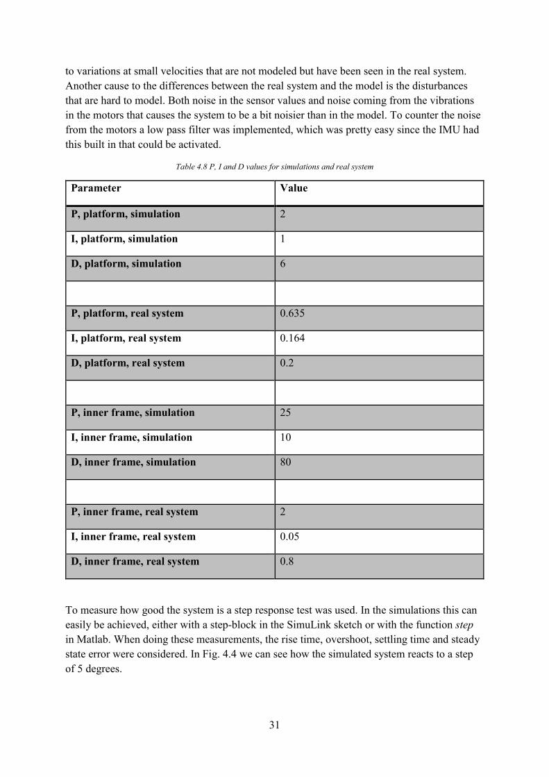
31

to variations at small velocities that are not modeled but have been seen in the real system.

Another cause to the differences between the real system and the model is the disturbances

that are hard to model. Both noise in the sensor values and noise coming from the vibrations

in the motors that causes the system to be a bit noisier than in the model. To counter the noise

from the motors a low pass filter was implemented, which was pretty easy since the IMU had

this built in that could be activated.

Table 4.8 P, I and D values for simulations and real system

Parameter Value

P, platform, simulation 2

I, platform, simulation 1

D, platform, simulation 6

P, platform, real system 0.635

I, platform, real system 0.164

D, platform, real system 0.2

P, inner frame, simulation 25

I, inner frame, simulation 10

D, inner frame, simulation 80

P, inner frame, real system 2

I, inner frame, real system 0.05

D, inner frame, real system 0.8

To measure how good the system is a step response test was used. In the simulations this can

easily be achieved, either with a step-block in the SimuLink sketch or with the function step

in Matlab. When doing these measurements, the rise time, overshoot, settling time and steady

state error were considered. In Fig. 4.4 we can see how the simulated system reacts to a step

of 5 degrees.

32

Fig. 4.4 Simulated step response of 5 degrees

As we can see that both systems can handle the step good. We see that they are fast and with

low or no overshoot. In table 4.9 we can see the desired values for the system and in table

4.10 we can see the simulated values for both PIDs.

Table 4.9 Desired results from the system

Parameter Value

Rise time (s) 0.5

Settling time (s) 1.5

Overshoot (%) 10

Steady state error (%) 2

33

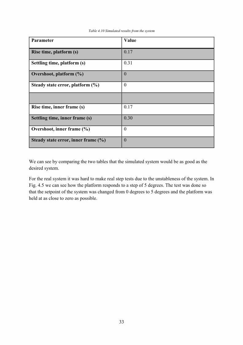
Table 4.10 Simulated results from the system

Parameter Value

Rise time, platform (s) 0.17

Settling time, platform (s) 0.31

Overshoot, platform (%) 0

Steady state error, platform (%) 0

Rise time, inner frame (s) 0.17

Settling time, inner frame (s) 0.30

Overshoot, inner frame (%) 0

Steady state error, inner frame (%) 0

We can see by comparing the two tables that the simulated system would be as good as the

desired system.

For the real system it was hard to make real step tests due to the unstableness of the system. In

Fig. 4.5 we can see how the platform responds to a step of 5 degrees. The test was done so

that the setpoint of the system was changed from 0 degrees to 5 degrees and the platform was

held at as close to zero as possible.

34

Fig. 4.5 Step response for the inner platform of 5 degrees

As we can see the response is pretty good, however the plot is a bit misleading because it does

not show how the system responds to disturbances. Unfortunately, such data was too hard to

capture in plots via Matlab, but the oscillation around the setpoint grew larger with time in

this case.

5 Conclusions and future work

5.1 System identification/Simulations

The system identification used in this project could be improved in the future. The equations

that were used was found in more than one source, but the parameters that were used in the

simulations were found by experiments. It was realized after the decision to use the chosen

motors, that the manufacturer did not provide the needed parameters on the motors. Before

deciding on the motors, it should have been investigated which parameters were needed for

the modelling equations. This is suggested for future work.

5.2 Regulator

The regulator that was designed by simulations worked as intended. In chapter 4.3.2 we can

see the results are satisfactory with the wanted system. However, it can be concluded that the

complete system did not behave as the simulations would suggest and therefore the simulated

regulator did not perform as well in a real environment as in the simulations. This was mostly

because of disturbances that were hard to model and simulate. However, based on the

35

simulations, if a prototype with better mechanics could be designed, a PID regulator would

give satisfactory results in controlling the system.

5.3 Mechanics

When working with this project the construction of the prototype has taken by far the most of

the time. This is because I didn’t have any previous knowledge or experience in constructing

these types of machines. In retrospect the prototype should probably had been made by

someone with more knowledge in the field so that the project could have focused more on the

software design and the system identification.

5.4 Complete system

The final constructed system did not perform with as good stability as expected. Most of the

problems stem from faults in the construction and the hardware. As mentioned in the previous

chapter the chosen motors were not optimal for this project and in the future a better analysis

on which type of motors that could be used, should be done.

36

References

[1] Wikipedia, "Gimbal," 26 March 2018. [Online]. Available: https://en.wikipedia.org/wiki/Gimbal.

[Accessed 28 May 2018].

[2] J. M. Hilkert, ”Inertially stabilized platform technology Concepts and Principles,” IEEE Control

Systems Magazine, vol. 28, nr 1, pp. 26-46, 2008.

[3] L. Payne, "The Modern Industrial Workhorse: PID Controllers," Techbriefs, 1 July 2014.

[Online]. Available: https://www.techbriefs.com/component/content/article/ntb/features/feature-

articles/20013. [Accessed 24 May 2018].

[4] P. Avery, "Introduction to PID control," MachineDesign, 1 Mars 2009. [Online]. Available:

http://www.machinedesign.com/sensors/introduction-pid-control. [Accessed 24 May 2018].

[5] MathWorks, "PID Tuner," MathWorks, [Online]. Available:

https://se.mathworks.com/help/control/ref/pidtuner-app.html. [Accessed 9 April 2018].

[6] B. Messner, D. Tilbury, R. Hill and J. Taylor, "DC Motor Speed: System Modeling," Control

tutorials for Matlab and SimuLink, 2017. [Online]. Available:

http://ctms.engin.umich.edu/CTMS/index.php?example=MotorSpeed&section=SystemModeling.

[Accessed 1 January 2018].

[7] I. Virgala and M. Keleman, "Experimental Friction Identification of a DC Motor," International

Journal of Mechanics and Applications, vol. 3, no. 1, pp. 26-30, Mars 2013.

[8] S. T. Thornton and J. B. Marion, "Dynamics of Rigid Bodies," in Classical dynamics of particles

and system, Belmont, CA, Brooks/Cole - Thompson Learning, 2004, pp. 411-463.

[9] P. Korondi, J. Halas, K. Samu, A. Bojtos and P. Tamás, "Models of friction," in Robot

applications, Budapest, BME MOGI, 2014, pp. 118-130.

[10] C. Nordling and J. Österman, Physics handbook for science and engineering, Lund:

Studentlitteratur AB, 2006.

[11] G. Wetzstein, "Inertial Measurement Units I," [Online]. Available:

https://stanford.edu/class/ee267/lectures/lecture9.pdf. [Accessed 18 May 2018].

[12] S. Walsh, "Processing data from MPU-6050," Sam's blog, 18 July 2014. [Online]. Available:

http://samselectronicsprojects.blogspot.se/2014/07/processing-data-from-mpu-6050.html.

[Accessed 26 February 2018].

[13] M. Pedley, "Tilt Sensing Using a Three-Axis Accelerometer," Mars 2013. [Online]. Available:

https://www.nxp.com/docs/en/application-note/AN3461.pdf. [Accessed 26 February 2018].

37

[14] T. Glad and L. Ljung, Reglerteori - Flervariabla och olinjära metoder, Lund: Studentlitteratur

AB, 2003.

[15] G. Welch och G. Bishop, ”An Introduction to the Kalman Filter,” Department of Computer

Science University of North Carolina at CHapel Hill, Chapel Hill, NC, 2006.

[16] R. Faragher, ”Understanding the Basis of the Kalman Filter Via a Simple and Intuitive

Derivation [Lecture Notes],” IEEE Signal Processing Magazine, vol. 29, nr 5, pp. 128-132,

2012.

[17] Arduino, "Arduino Mega 2560 Rev3," Arduino store, [Online]. Available:

https://store.arduino.cc/arduino-mega-2560-rev3. [Accessed 2 May 2018].

[18] Sparkfun, ”Sparkfun.com,” [Online]. Available: https://www.sparkfun.com/products/11028.

[Använd 19 June 2018].

[19] Transmotec, ”transmotec.se,” [Online]. Available: https://www.transmotec.se/wp-

content/uploads/2017/05/MD3FN-3270-CVC-26-29-dia-20.jpg. [Använd 19 June 2018].

[20] CTC, "Measuring Motor Parameters," [Online]. Available: http://support.ctc-

control.com/customer/elearning/younkin/motorParameters.pdf. [Accessed 12 March 2018].

[21] Arduino, "Arduino Software (IDE)," Arduino, 7 September 2015. [Online]. Available:

https://www.arduino.cc/en/Guide/Environment. [Accessed 3 May 2018].

[22] Brio, "Labyrint Brio Butik," [Online]. Available: http://www.brio.se/produkter/alder/fran-6-

ar/labyrint. [Accessed 24 May 2018].

[23] B&H photo and video, "Ikan EC1 Beholder 3-Axis Handheld Gimbal Stabilizer," [Online].

Available: https://www.bhphotovideo.com/c/product/1278590-

REG/ikan_ec1_beholder_handheld_3_axis.html. [Accessed 24 May 2018].

[24] B. Beauregard, "Arduino PID Library," [Online]. Available:

https://playground.arduino.cc/Code/PIDLibrary. [Accessed 27 March 2018].

[25] D. Collins, "FAQ: What's the difference between torque constant, back EMF constant, and motor

constant," Motion control tips, 5 April 2017. [Online]. Available:

https://www.motioncontroltips.com/faq-difference-between-torque-back-emf-motor-constant/.

[Accessed 15 March 2018].

38

Appendices A. Full derivation for DC motor transfer function

In this chapter a full derivation of the DC motor transfer function, described in chapter 2.2,

will be given. A mathematically expression for the relation of the voltage in a DC motor can

be written as

��� = �� + ���

��+ ���� (A.1)

Where VEMF can be expressed as

���� = ���̇ (A.2)

With KE as the back-EMF constant. These two equations combined, gives us the following

�� + ���

��= ��� − ���̇ (A.3)

The transfer function relates the applied voltage, VIN, to the angular velocity of the motor, �̇.

To find this relation we will use the relation between the torque of the motor and the armature

current of the motor, written as

�� = ��� (A.4)

With KT called the torque constant. The torque can then be related to the angular velocity,

since torque is equal to the inertia multiplied with the angular acceleration, written as

���� = ��̈ (A.5)

The total torque of a DC motor is then the motor torque minus the friction torque, which is

expressed as

���� = �� − �� (A.6)

By combining these equations, we get an expression with the angular acceleration and the

armature current, which is written as

��̈ = ��� − ��(�̇) (A.7)

Now we can use the Laplace transform on equation (A.3) and equation (A.7), we get the

following expressions

���̇ = ��� − ����̇� ⇒ � =���̇���(�̇)

�� (A.8)

��� + �� = ��� − ���̇ ⇒ � =�������̇

���� (A.9)

39

Since both equations are equal to I, they can be combined into an equation which is only

dependent on the voltage, the angular velocity and constants. This can be written as

���̇���(�̇)

��=

�������̇

���� (A.10)

Finally, we can put the angular velocity and the voltage into a relation, which is the transfer

function and can be expressed as

�̇

���=

��

(����)��������̇�������

(A.11)

B. Proof that KT equals KE in SI-units

When the back-EMF constant is determined, so is the motor torque constant. This can be

shown by applying the law of conservation of energy. In Fig. B.1 the circuit of the DC-motor

can be seen [25].

Fig. B.1 Electrical circuit of a DC-motor

The electrical power in can be expressed as

��� = ��� � (B.1)

From Fig. B.1 and Kirschoff’s law, we get the equation for Vin, written as

��� = �� + ���� = �� + ��� (B.2)

We substituted VEMF to express it in Ke instead as explained previously. Now to get the power

that goes into the system, the voltage needs to be multiplied with the current, I, expressed as

���� = ��� = ��� + ���� (B.3)

Now the power output needs to be calculated and that power can be calculated by multiplying

the torque, T, with the angular velocity, �. Since the torque is equal to the motor torque

constant multiplied with the current they can be substituted, which is written as

40

����,���������� = �� = ���� (B.4)

Before the power output is equal to the power input, the electrical losses due to resistance in

the circuit needs to be added.

���� = ��� + ���� (B.5)

Now the power output is set equal to the power input and can be expressed as follows

��� = ��� + ���� = ���� = ��� + ���� (B.6)

This gives, after simplifying

�� = �� (B.7)