heizer omawe ch14
TRANSCRIPT
14 - 1
14 Material Requirements Planning (MRP) and ERP
PowerPoint presentation to accompany PowerPoint presentation to accompany
Heizer, Render, and Al-Zu’biHeizer, Render, and Al-Zu’bi
Operations Management, Operations Management, Arab World EditionArab World Edition
Original PowerPoint slides by Jeff HeylOriginal PowerPoint slides by Jeff Heyl
Adapted by Zu’bi Al-Zu’biAdapted by Zu’bi Al-Zu’bi
14 - 2
OutlineOutline Company Profile: Jordan
Company for Dead Sea Products Dependent Demand Dependent Inventory Model
Requirements Master Production Schedule Bills of Material Accurate Inventory Records Purchase Orders Outstanding Lead Times for Components
14 - 3
Outline – ContinuedOutline – Continued
MRP Structure Safety Stock
MRP Management MRP Dynamics MRP and JIT
14 - 4
Outline – ContinuedOutline – Continued
Lot-Sizing Techniques Lot-for-lot Economic order quantity Part Period Balancing Wagner-Whitin Procedure Lot-Sizing Summary
Extensions of MRP Material Requirements Planning II (MRP II) Closed-Loop MRP Capacity Planning
14 - 5
Outline – ContinuedOutline – Continued
MRP In Services Distribution Resource Planning (DRP)
Enterprise Resource Planning (ERP) Advantages and Disadvantages of
ERP Systems ERP in the Service Sector
14 - 6
Learning ObjectivesLearning Objectives
When you complete this chapter you should be able to:When you complete this chapter you should be able to:
1. Develop a product structure2. Build a gross requirements plan3. Build a net requirements plan4. Determine lot sizes for lot-for-lot,
EOQ, and PPB
14 - 7
Learning ObjectivesLearning Objectives
When you complete this chapter you should be able to:When you complete this chapter you should be able to:
5. Describe MRP II6. Describe closed-loop MRP7. Describe ERP
14 - 8
Jordan Company for Dead Sea ProductsJordan Company for Dead Sea Products
One of the largest manufacturers of Dead Sea products in Jordan – La Cure
International competitor 52 major brands sold to 53
countries around the world
14 - 9
Jordan company for Dead Sea ProductsJordan company for Dead Sea Products
Four Key Tasks Material plan must meet both the
requirements of the master schedule and the capabilities of the production facility
Plan must be executed as designed Minimize inventory investment Maintain excellent record integrity
14 - 10
Dependent DemandDependent Demand
For any product for which a schedule For any product for which a schedule can be established, dependent can be established, dependent
demand techniques should be useddemand techniques should be used
14 - 11
Dependent DemandDependent Demand
Benefits of MRP1. Better response to customer
orders2. Faster response to market
changes3. Improved utilization of facilities
and labor4. Reduced inventory levels
14 - 12
Dependent DemandDependent Demand
The demand for one item is related to the demand for another item
Given a quantity for the end item, the demand for all parts and components can be calculated
In general, used whenever a schedule can be established for an item
MRP is the common technique
14 - 13
Dependent DemandDependent Demand
Benefits of MRP Better response to customer
orders Faster response to market changes Improved utilization of facilities
and labor Reduced inventory levels
14 - 14
Dependent DemandDependent Demand
1. Master production schedule2. Specifications or bill of material3. Inventory availability4. Purchase orders outstanding5. Lead times
Effective use of dependent demand inventory models requires the following
14 - 15
Master Production Schedule (MPS)Master Production Schedule (MPS) Specifies what is to be made and when Must be in accordance with the aggregate
production plan Inputs from financial plans, customer
demand, engineering, supplier performance As the process moves from planning to
execution, each step must be tested for feasibility
The MPS is the result of the production planning process
14 - 16© 2013 Pearson Education
Master Production Schedule (MPS)Master Production Schedule (MPS)
MPS is established in terms of specific products
Schedule must be followed for a reasonable length of time
The MPS is quite often fixed or frozen in the near term part of the plan
The MPS is a rolling schedule The MPS is a statement of what is to be
produced, not a forecast of demand
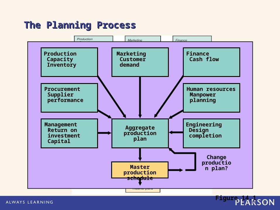
14 - 17Figure 14.1
Change production
plan?Master production schedule
ManagementReturn oninvestmentCapital
EngineeringDesigncompletion
Aggregate production
plan
ProcurementSupplierperformance
Human resourcesManpowerplanning
ProductionCapacityInventory
MarketingCustomerdemand
FinanceCash flow
The Planning ProcessThe Planning Process
14 - 18
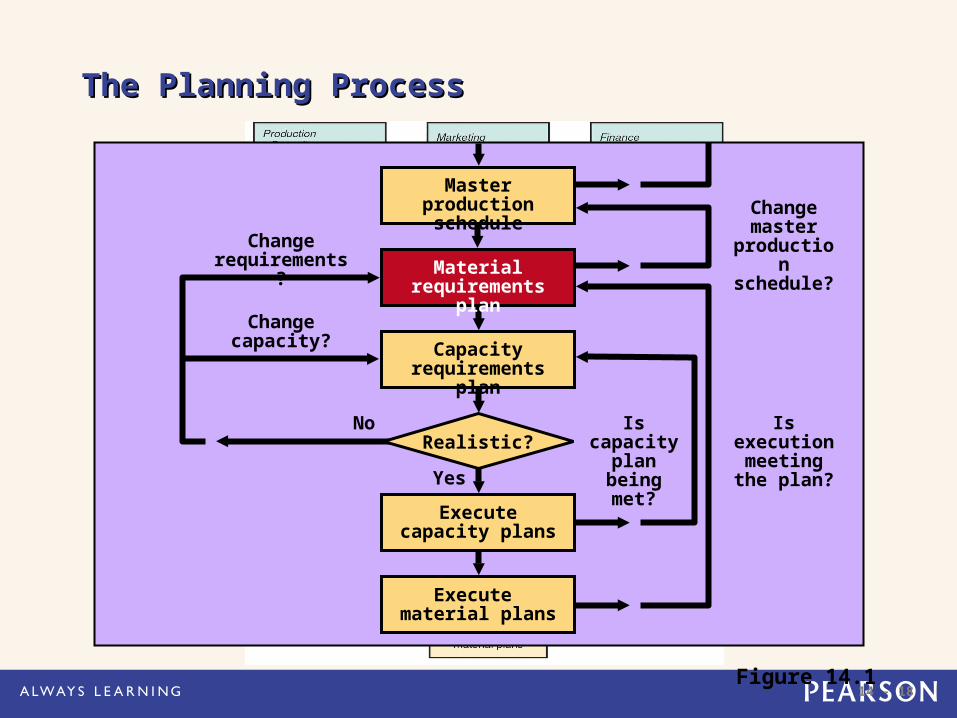
The Planning ProcessThe Planning Process
Figure 14.1
Is capacity plan being
met?
Is execution
meeting the plan?
Change master
production schedule?
Change capacity?
Change requirements?
No
Execute material plans
Execute capacity plans
Yes
Realistic?
Capacity requirements plan
Material requirements plan
Master production schedule
14 - 19
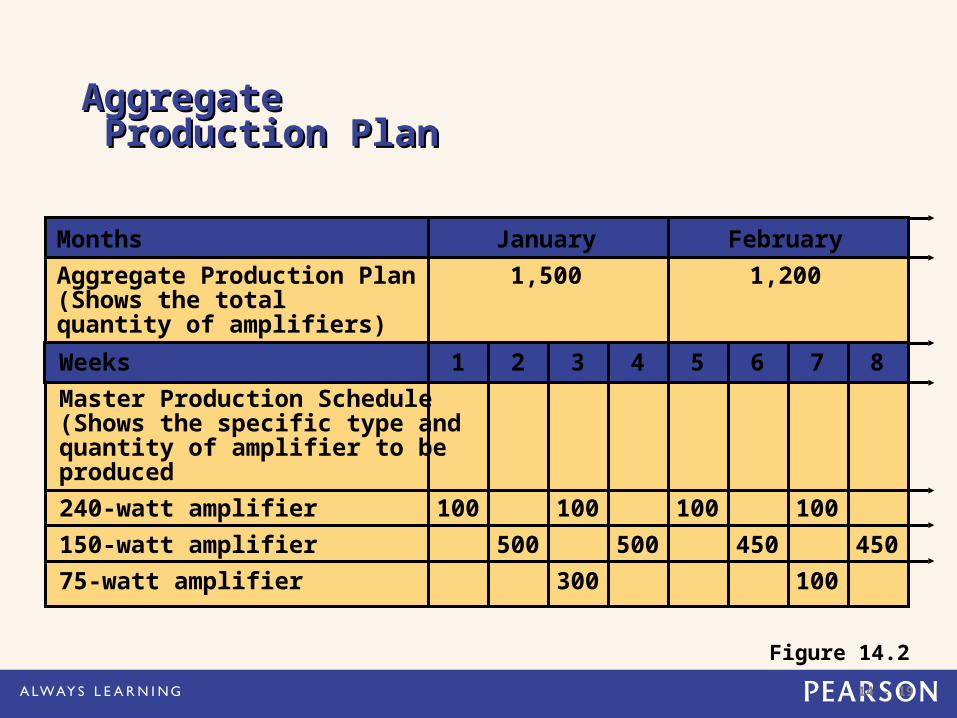
AggregateAggregate Production Plan Production Plan
Months January FebruaryAggregate Production Plan 1,500 1,200(Shows the totalquantity of amplifiers)Weeks 1 2 3 4 5 6 7 8Master Production Schedule(Shows the specific type andquantity of amplifier to beproduced240-watt amplifier 100 100 100 100150-watt amplifier 500 500 450 45075-watt amplifier 300 100
Figure 14.2
14 - 20
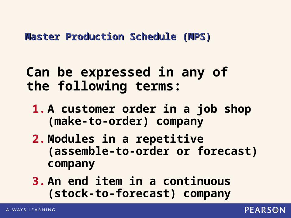
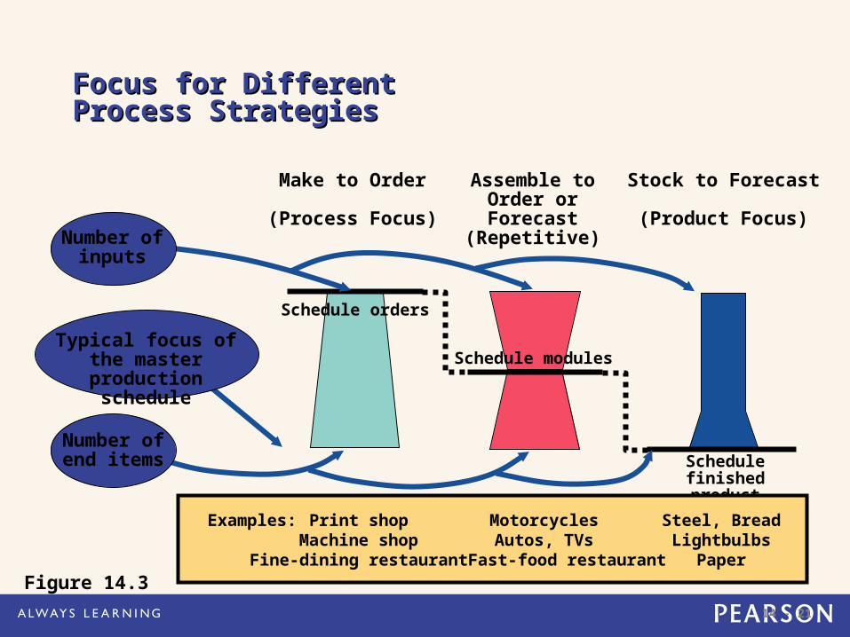
Master Production Schedule (MPS)Master Production Schedule (MPS)
1. A customer order in a job shop (make-to-order) company
2. Modules in a repetitive (assemble-to-order or forecast) company
3. An end item in a continuous (stock-to-forecast) company
Can be expressed in any of the following terms:
14 - 21
Focus for Different Focus for Different Process StrategiesProcess Strategies
Stock to Forecast
(Product Focus)
Schedule finished product
Assemble to Order or Forecast(Repetitive)
Schedule modules
Make to Order
(Process Focus)
Schedule orders
Examples: Print shop Motorcycles Steel, BreadMachine shop Autos, TVs Lightbulbs
Fine-dining restaurant Fast-food restaurant Paper
Typical focus of the master production
schedule
Number of inputs
Number of end items
Figure 14.3
14 - 22
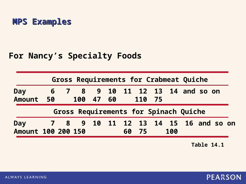
MPS ExamplesMPS Examples
Gross Requirements for Crabmeat Quiche
Gross Requirements for Spinach Quiche
Day 6 7 8 9 10 11 12 13 14 and so onAmount 50 100 47 60 110 75
Day 7 8 9 10 11 12 13 14 15 16 and so onAmount 100 200 150 60 75 100
Table 14.1
For Nancy’s Specialty Foods
14 - 23
Bills of Material (BOM)Bills of Material (BOM)
List of components, ingredients, and materials needed to make product
Provides product structure Items above given level are called
‘parents’ Items below given level are called
‘children’
14 - 24
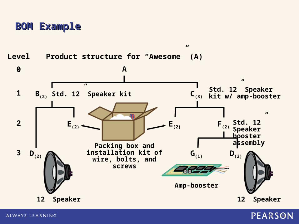
BOM ExampleBOM Example
B(2) Std. 12” Speaker kit C(3)Std. 12” Speaker kit w/ amp-booster1
E(2)E(2) F(2)
Packing box and installation kit of wire,
bolts, and screws
Std. 12” Speaker booster assembly
2
D(2)
12” Speaker
D(2)
12” Speaker
G(1)
Amp-booster
3
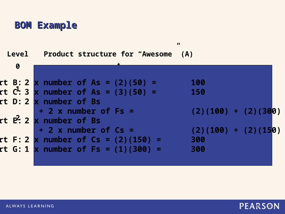
Product structure for “Awesome” (A)A
Level0
14 - 25
BOM ExampleBOM Example
B(2) Std. 12” Speaker kit C(3)Std. 12” Speaker kit w/ amp-booster1
E(2)E(2) F(2)
Packing box and installation kit of wire,
bolts, and screws
Std. 12” Speaker booster assembly
2
Product structure for “Awesome” (A)A
Level0
Part B: 2 x number of As = (2)(50) = 100Part C: 3 x number of As = (3)(50) = 150Part D: 2 x number of Bs
+ 2 x number of Fs = (2)(100) + (2)(300) = 800Part E: 2 x number of Bs
+ 2 x number of Cs = (2)(100) + (2)(150) = 500Part F: 2 x number of Cs = (2)(150) = 300Part G: 1 x number of Fs = (1)(300) = 300
14 - 26
Bills of MaterialBills of Material
Modular Bills Modules are not final products but
components that can be assembled into multiple end items
Can significantly simplify planning and scheduling
14 - 27
Bills of MaterialBills of Material
Planning Bills Also called “pseudo” or super bills Created to assign an artificial parent
to the BOM Used to group subassemblies to
reduce the number of items planned and scheduled
Used to create standard ‘kits’ for production
14 - 28
Bills of MaterialBills of Material
Phantom BillsDescribe subassemblies that exist
only temporarilyAre part of another assembly and
never go into inventory Low-Level Coding
Item is coded at the lowest level at which it occurs
BOMs are processed one level at a time

14 - 29
Accurate Inventory RecordsAccurate Inventory Records
Accurate inventory records are absolutely required for MRP (or any dependent demand system) to operate correctly
Generally MRP systems require more than 99% accuracy
14 - 30
Purchase Orders OutstandingPurchase Orders Outstanding
Outstanding purchase orders must accurately reflect quantities and scheduled receipts
14 - 31
Lead TimesLead Times
The time required to purchase, produce, or assemble an item For production – the sum of the
order, wait, move, setup, store, and run times
For purchased items – the time between the recognition of a need and the availability of the item for production
14 - 32
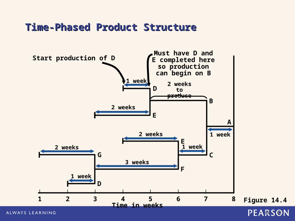
Time-Phased Product StructureTime-Phased Product Structure
| | | | | | | |
1 2 3 4 5 6 7 8Time in weeks
F
2 weeks
3 weeks
1 week
A
2 weeks
1 weekD
E
2 weeks
D
G
1 week
Start production of DMust have D and E completed here so
production can begin on B
Figure 14.4
1 week
2 weeks to produce
B
C
E
14 - 33
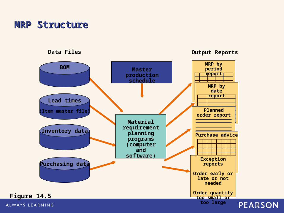
MRP StructureMRP Structure
Figure 14.5
Output Reports
MRP by period report
MRP by date report
Planned order report
Purchase advice
Exception reports
Order early or late or not needed
Order quantity too small or too large
Data Files
Purchasing data
BOM
Lead times
(Item master file)
Inventory data
Masterproduction schedule
Material requirement
planning programs
(computer and software)
14 - 34
Determining Gross RequirementsDetermining Gross Requirements
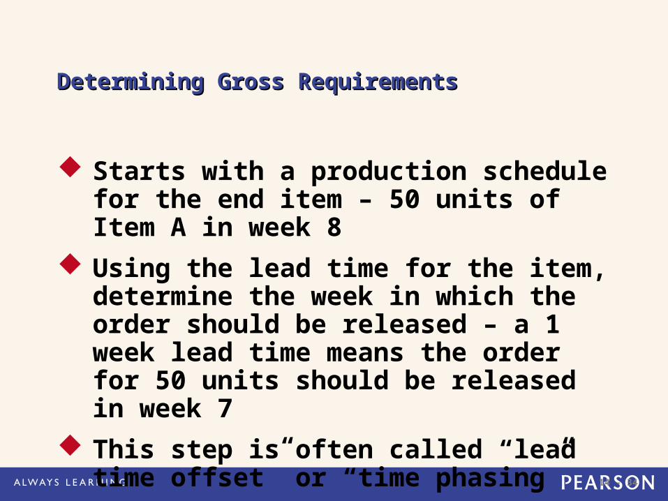
Starts with a production schedule for the end item – 50 units of Item A in week 8
Using the lead time for the item, determine the week in which the order should be released – a 1 week lead time means the order for 50 units should be released in week 7
This step is often called “lead time offset” or “time phasing”
14 - 35
Determining Gross RequirementsDetermining Gross Requirements
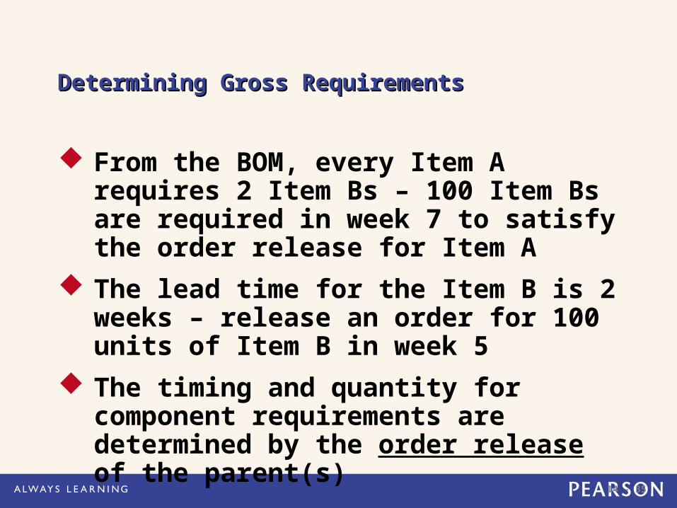
From the BOM, every Item A requires 2 Item Bs – 100 Item Bs are required in week 7 to satisfy the order release for Item A
The lead time for the Item B is 2 weeks – release an order for 100 units of Item B in week 5
The timing and quantity for component requirements are determined by the order release of the parent(s)
14 - 36
Determining Gross RequirementsDetermining Gross Requirements
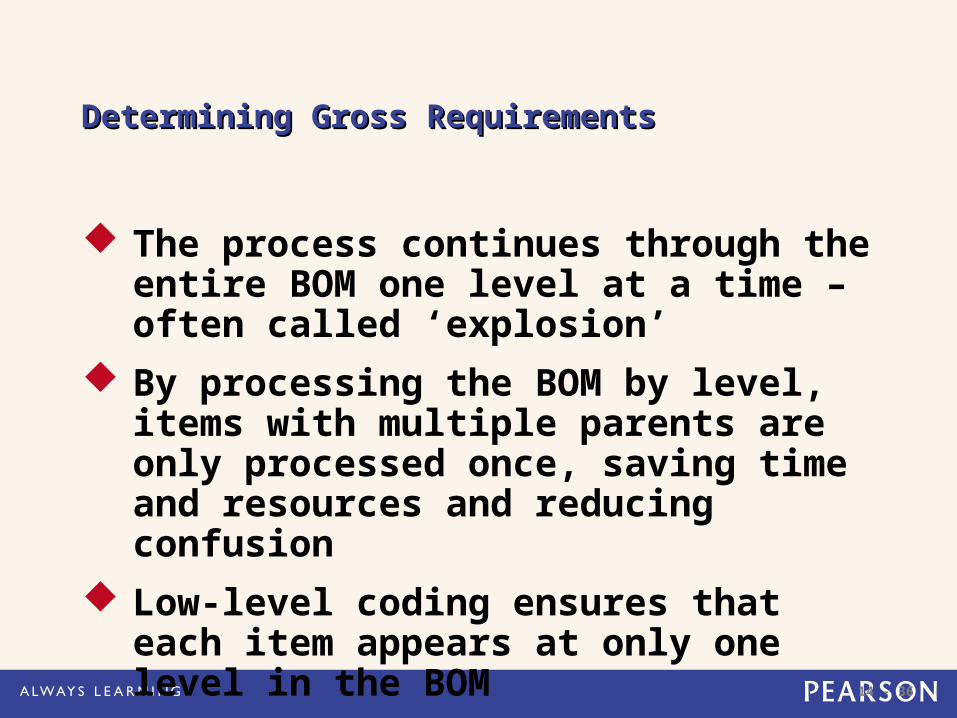
The process continues through the entire BOM one level at a time – often called ‘explosion’
By processing the BOM by level, items with multiple parents are only processed once, saving time and resources and reducing confusion
Low-level coding ensures that each item appears at only one level in the BOM
14 - 37
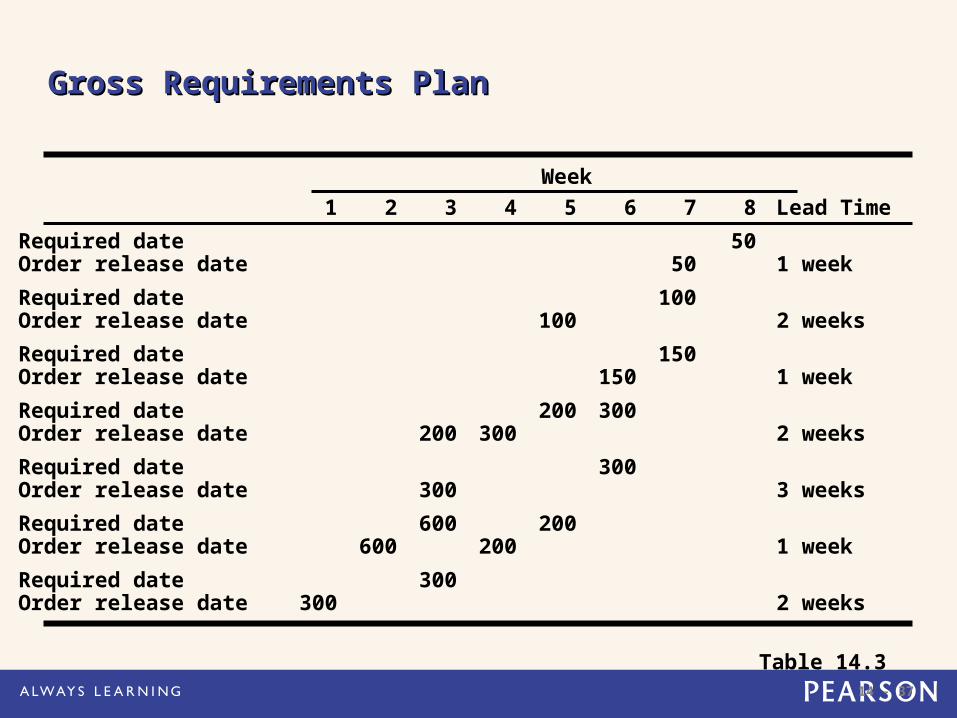
Gross Requirements PlanGross Requirements Plan
Table 14.3
Week1 2 3 4 5 6 7 8 Lead Time
A. Required date 50Order release date 50 1 week
B. Required date 100Order release date 100 2 weeks
C. Required date 150Order release date 150 1 week
E. Required date 200 300Order release date 200 300 2 weeks
F. Required date 300Order release date 300 3 weeks
G. Required date 600 200Order release date 600 200 1 week
G. Required date 300Order release date 300 2 weeks
14 - 38
Net Requirements PlanNet Requirements Plan
Figure 14.6
14 - 39
Net Requirements PlanNet Requirements Plan
Figure 14.6

14 - 40
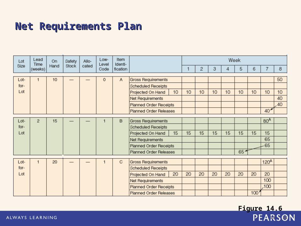
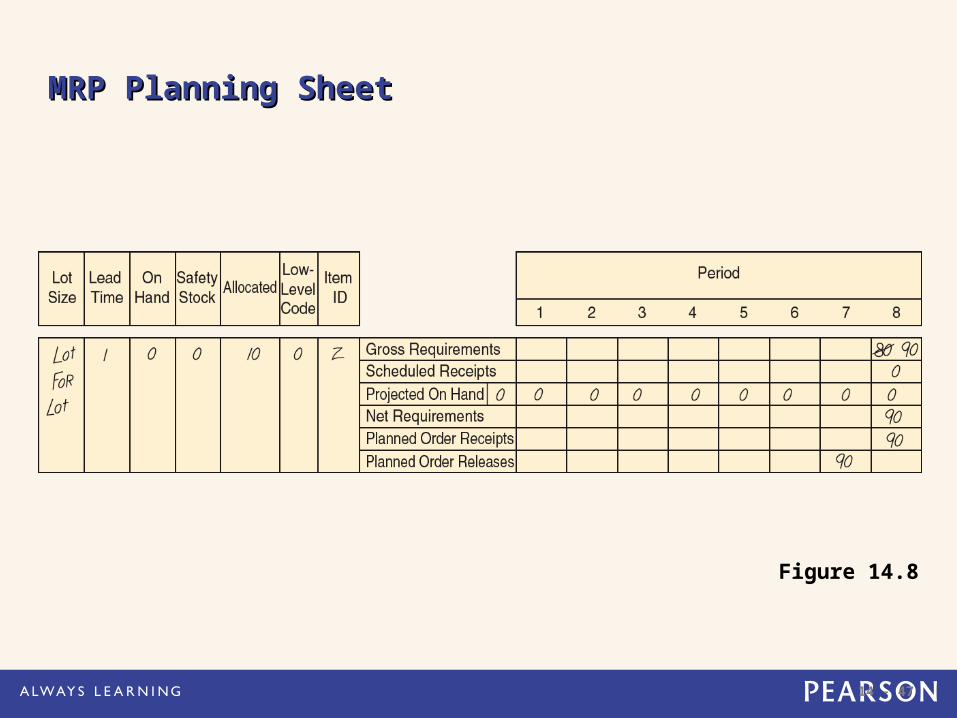
Determining Net RequirementsDetermining Net Requirements
Starts with a production schedule for the end item – 50 units of Item A in week 8
Because there are 10 Item As on hand, only 40 are actually required – (net requirement) = (gross requirement - on- hand inventory)
The planned order receipt for Item A in week 8 is 40 units – 40 = 50 - 10
14 - 41
Determining Net RequirementsDetermining Net Requirements
Following the lead time offset procedure, the planned order release for Item A is now 40 units in week 7
The gross requirement for Item B is now 80 units in week 7
There are 15 units of Item B on hand, so the net requirement is 65 units in week 7
A planned order receipt of 65 units in week 7 generates a planned order release of 65 units in week 5
14 - 42
Determining Net RequirementsDetermining Net Requirements
A planned order receipt of 65 units in week 7 generates a planned order release of 65 units in week 5
The on-hand inventory record for Item B is updated to reflect the use of the 15 items in inventory and shows no on-hand inventory in week 8
This is referred to as the Gross-to-Net calculation and is the third basic function of the MRP process
14 - 43
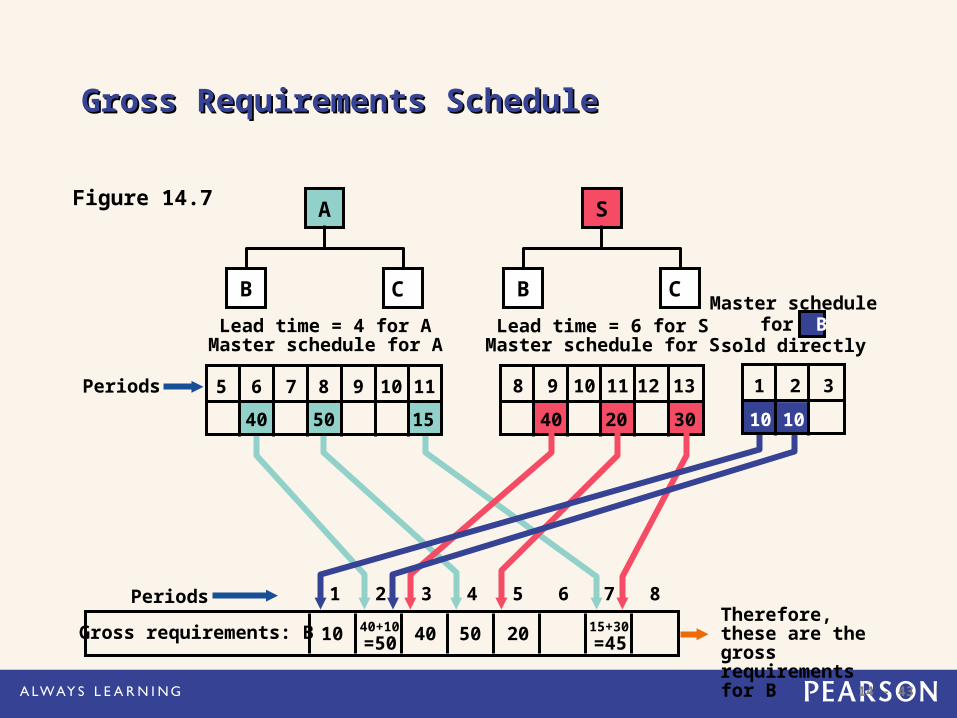
S
B C
12 138 9 10 11
20 3040
Lead time = 6 for SMaster schedule for S
Gross Requirements ScheduleGross Requirements Schedule
Figure 14.7
1 2 3
10 10
Master schedulefor B
sold directly
Periods
Therefore, these are the gross requirements for B
Gross requirements: B 10 40 50 2040+10 15+30=50 =45
1 2 3 4 5 6 7 8Periods
A
B CLead time = 4 for A
Master schedule for A
5 6 7 8 9 10 11
40 1550
14 - 44
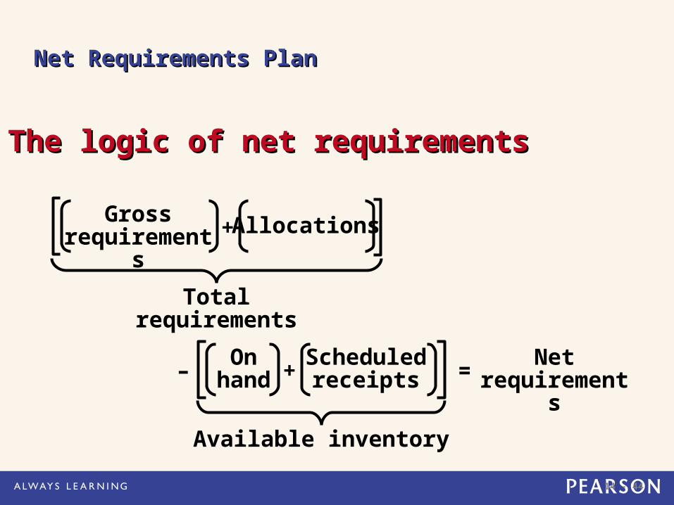
Net Requirements PlanNet Requirements Plan
The logic of net requirementsThe logic of net requirements
Available inventory
Net requirements
On hand
Scheduled receipts+– =
Total requirements
Gross requirements Allocations+
14 - 45
Safety StockSafety Stock
• BOMs and inventory rocords may not be perfect
• Some safety stock would be prudent, but should be
• Minimized
• Built into the projected on-hand inventory of the MRP logic
14 - 46
Safety StockSafety Stock
• BOMs, inventory records, purchase and production quantities may not be perfect
• Consideration of safety stock may be prudent
• Should be minimized and ultimately eliminated
• Typically built into projected on-hand inventory
14 - 47
MRP Planning SheetMRP Planning Sheet
Figure 14.8
14 - 48
MRP DynamicsMRP Dynamics
MRP is a dynamic system Facilitates replanning when changes occur
Regenerating Net change
System nervousness can result from too many changes
Time fences put limits on replanning Pegging links each item to its parent
allowing effective analysis of changes
14 - 49
MRP and JITMRP and JIT
MRP is a planning system that does not do detailed scheduling
MRP requires fixed lead times which might actually vary with batch size
JIT excels at rapidly moving small batches of material through the system
14 - 50
Finite Capacity SchedulingFinite Capacity Scheduling
MRP systems do not consider capacity during normal planning cycles
Finite capacity scheduling (FCS) recognizes actual capacity limits
By merging MRP and FCS, a finite schedule is created with feasible capacities which facilitates rapid material movement
14 - 51
Small Bucket ApproachSmall Bucket Approach
1. MRP “buckets” are reduced to daily or hourly2. Planned receipts are used internally to
sequence production3. Inventory is moved through the plant on a JIT
basis4. Completed products are moved to finished
goods inventory which reduces required quantities for subsequent planned orders
5. Back flushing based on the BOM is used to deduct inventory that was used in production
14 - 52
Balanced FlowBalanced Flow
Used in repetitive operations MRP plans are executed using
JIT techniques based on “pull” principles
Flows are carefully balanced with small lot sizes
14 - 53
SupermarketSupermarket
Items used by many products are held in a common area often called a supermarket
Items are withdrawn as needed Inventory is maintained using JIT
systems and procedures Common items are not planned by
the MRP system
14 - 54
Lot-Sizing TechniquesLot-Sizing Techniques
Lot-for-lot techniques order just what is required for production based on net requirements May not always be feasible If setup costs are high, lot-for-lot can
be expensive Economic order quantity (EOQ)
EOQ expects a known constant demand and MRP systems often deal with unknown and variable demand
14 - 55
Lot-Sizing TechniquesLot-Sizing Techniques
Part Period Balancing (PPB) looks at future orders to determine most economic lot size
The Wagner-Whitin algorithm is a complex dynamic programming technique Assumes a finite time horizon Effective, but computationally
burdensome
14 - 56
Lot-for-Lot ExampleLot-for-Lot Example
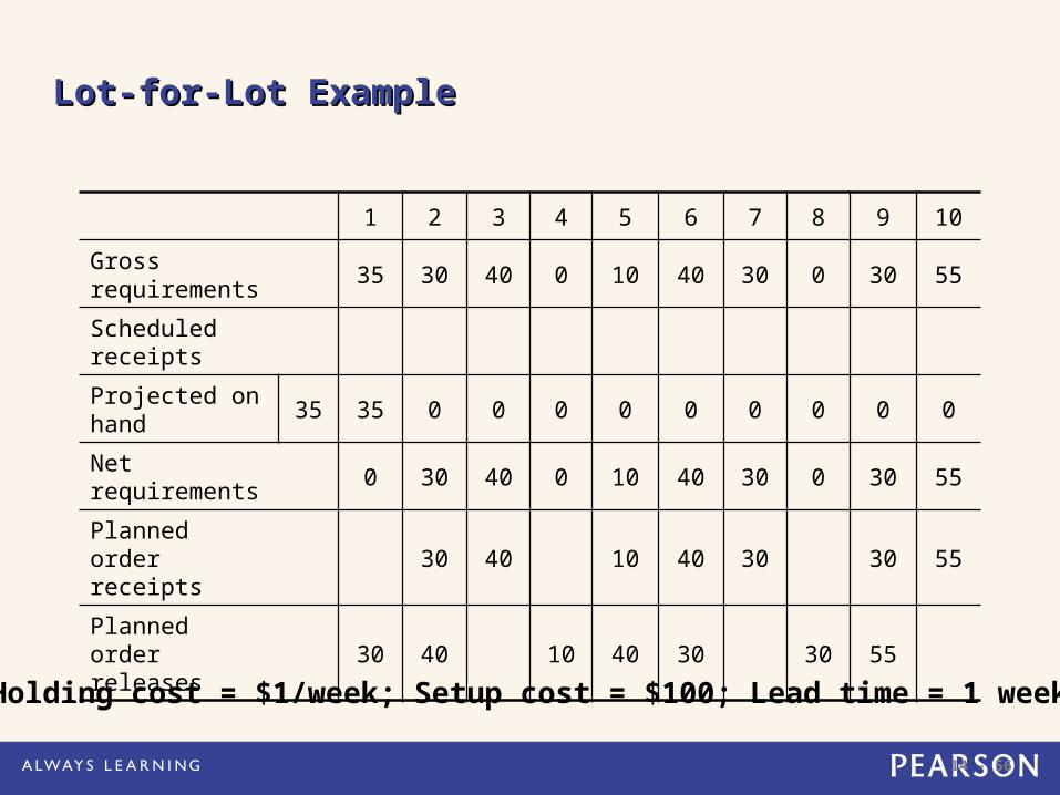
1 2 3 4 5 6 7 8 9 10Gross requirements 35 30 40 0 10 40 30 0 30 55
Scheduled receiptsProjected on hand 35 35 0 0 0 0 0 0 0 0 0
Net requirements 0 30 40 0 10 40 30 0 30 55
Planned order receipts 30 40 10 40 30 30 55
Planned order releases 30 40 10 40 30 30 55
Holding cost = $1/week; Setup cost = $100; Lead time = 1 week
14 - 57
Lot-for-Lot ExampleLot-for-Lot Example
1 2 3 4 5 6 7 8 9 10
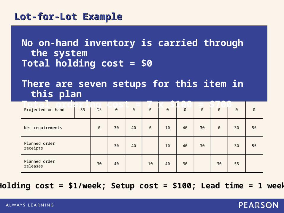
Gross requirements 35 30 40 0 10 40 30 0 30 55
Scheduled receipts
Projected on hand 35 35 0 0 0 0 0 0 0 0 0
Net requirements 0 30 40 0 10 40 30 0 30 55
Planned order receipts 30 40 10 40 30 30 55
Planned order releases 30 40 10 40 30 30 55
Holding cost = $1/week; Setup cost = $100; Lead time = 1 week
No on-hand inventory is carried through the systemTotal holding cost = $0
There are seven setups for this item in this planTotal ordering cost = 7 x $100 = $700
14 - 58
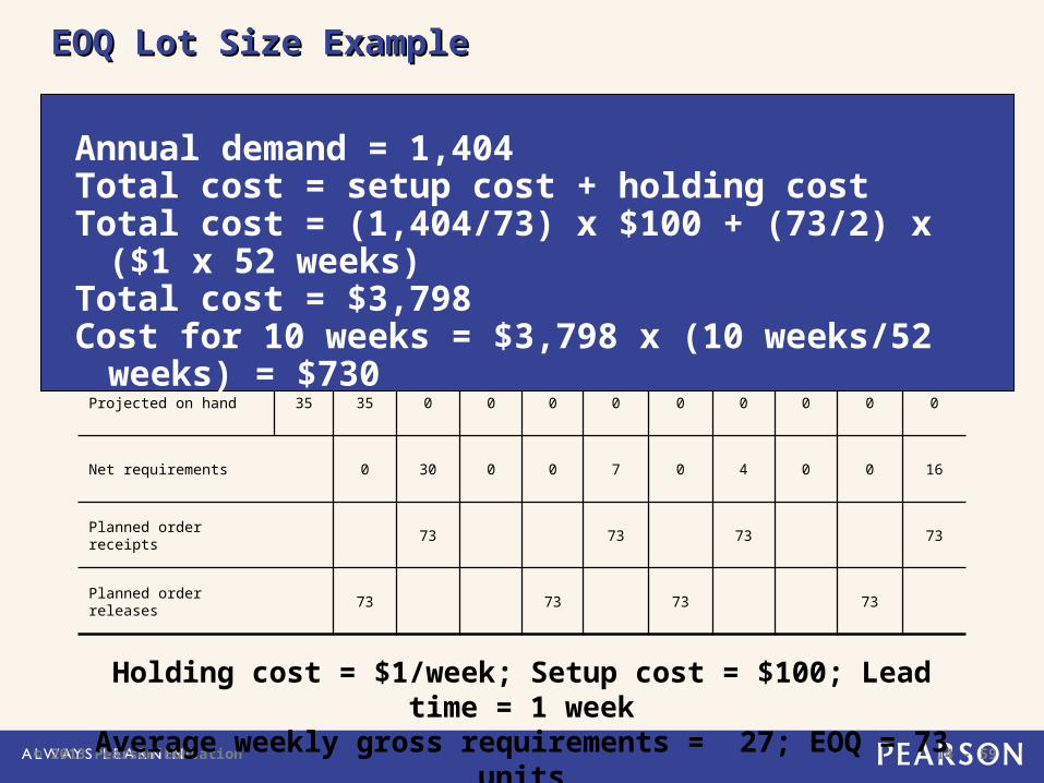
EOQ Lot Size ExampleEOQ Lot Size Example1 2 3 4 5 6 7 8 9 10
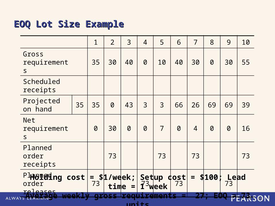
Gross requirements 35 30 40 0 10 40 30 0 30 55
Scheduled receipts
Projected on hand 35 35 0 43 3 3 66 26 69 69 39
Net requirements 0 30 0 0 7 0 4 0 0 16
Planned order receipts 73 73 73 73
Planned order releases 73 73 73 73
Holding cost = $1/week; Setup cost = $100; Lead time = 1 week
Average weekly gross requirements = 27; EOQ = 73 units
14 - 59© 2013 Pearson Education
EOQ Lot Size ExampleEOQ Lot Size Example
1 2 3 4 5 6 7 8 9 10
Gross requirements 35 30 40 0 10 40 30 0 30 55
Scheduled receipts
Projected on hand 35 35 0 0 0 0 0 0 0 0 0
Net requirements 0 30 0 0 7 0 4 0 0 16
Planned order receipts 73 73 73 73
Planned order releases 73 73 73 73
Holding cost = $1/week; Setup cost = $100; Lead time = 1 weekAverage weekly gross requirements = 27; EOQ = 73 units
Annual demand = 1,404Total cost = setup cost + holding costTotal cost = (1,404/73) x $100 + (73/2) x ($1 x 52 weeks)Total cost = $3,798Cost for 10 weeks = $3,798 x (10 weeks/52 weeks) =
$730
14 - 60
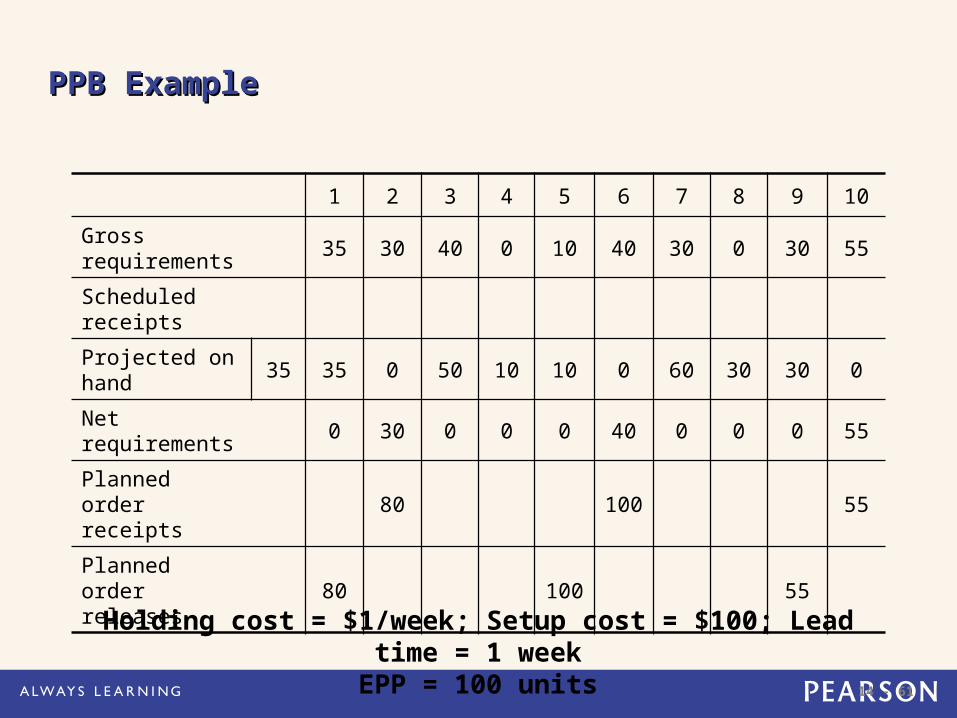
PPB ExamplePPB Example
1 2 3 4 5 6 7 8 9 10
Gross requirements 35 30 40 0 10 40 30 0 30 55
Scheduled receipts
Projected on hand 35
Net requirements
Planned order receipts
Planned order releases
Holding cost = $1/week; Setup cost = $100;EPP = 100 units
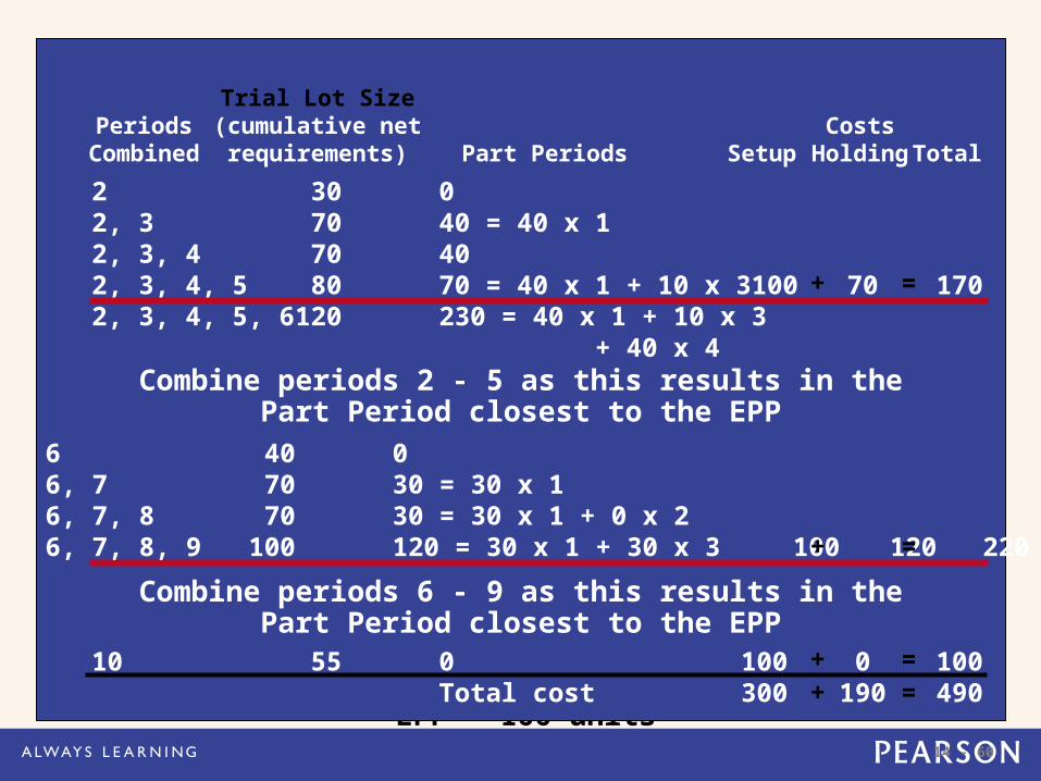
2 30 02, 3 70 40 = 40 x 12, 3, 4 70 402, 3, 4, 5 80 70 = 40 x 1 + 10 x 3 100 70 1702, 3, 4, 5, 6 120 230 = 40 x 1 + 10 x 3
+ 40 x 4
+ =
Combine periods 2 - 5 as this results in the Part Period closest to the EPP
Combine periods 6 - 9 as this results in the Part Period closest to the EPP
6 40 06, 7 70 30 = 30 x 16, 7, 8 70 30 = 30 x 1 + 0 x 26, 7, 8, 9 100 120 = 30 x 1 + 30 x 3 100 120 220+ =
10 55 0 100 0 100Total cost 300 190 490
+ =+ =
Trial Lot SizePeriods (cumulative net Costs
Combined requirements) Part Periods Setup Holding Total
14 - 61
PPB ExamplePPB Example
1 2 3 4 5 6 7 8 9 10Gross requirements 35 30 40 0 10 40 30 0 30 55
Scheduled receiptsProjected on hand 35 35 0 50 10 10 0 60 30 30 0
Net requirements 0 30 0 0 0 40 0 0 0 55
Planned order receipts 80 10
0 55
Planned order releases 80 100 55
Holding cost = $1/week; Setup cost = $100; Lead time = 1 weekEPP = 100 units
14 - 62
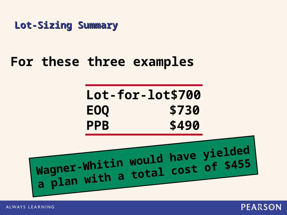
Lot-Sizing SummaryLot-Sizing Summary
For these three examples
Lot-for-lot $700EOQ $730PPB $490
Wagner-Whitin would have yielded a
plan with a total cost of $455
14 - 63
Lot-Sizing SummaryLot-Sizing Summary
In theory, lot sizes should be recomputed whenever there is a lot size or order quantity change
In practice, this results in system nervousness and instability
Lot-for-lot should be used when low-cost JIT can be achieved
14 - 64
Lot-Sizing SummaryLot-Sizing Summary
Lot sizes can be modified to allow for scrap, process constraints, and purchase lots
Use lot-sizing with care as it can cause considerable distortion of requirements at lower levels of the BOM
When setup costs are significant and demand is reasonably smooth, PPB, Wagner-Whitin, or EOQ should give reasonable results
14 - 65
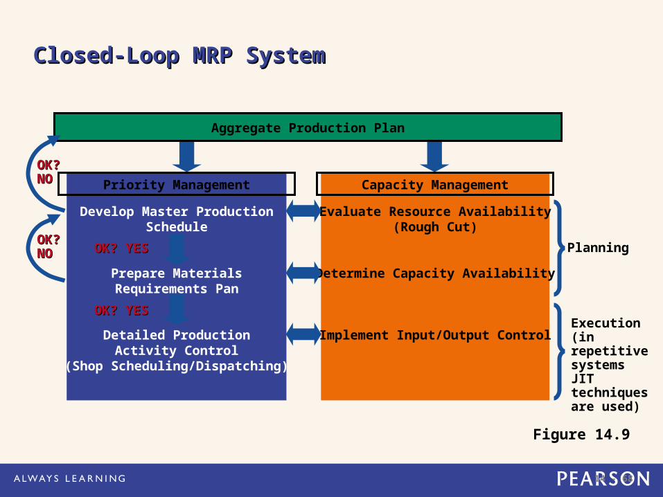
Extensions of MRPExtensions of MRP MRP II Closed-Loop MRP
MRP system provides input to the capacity plan, MPS, and production planning process
Capacity Planning MRP system generates a load report which
details capacity requirements This is used to drive the capacity planning
process Changes pass back through the MRP system
for rescheduling
14 - 66
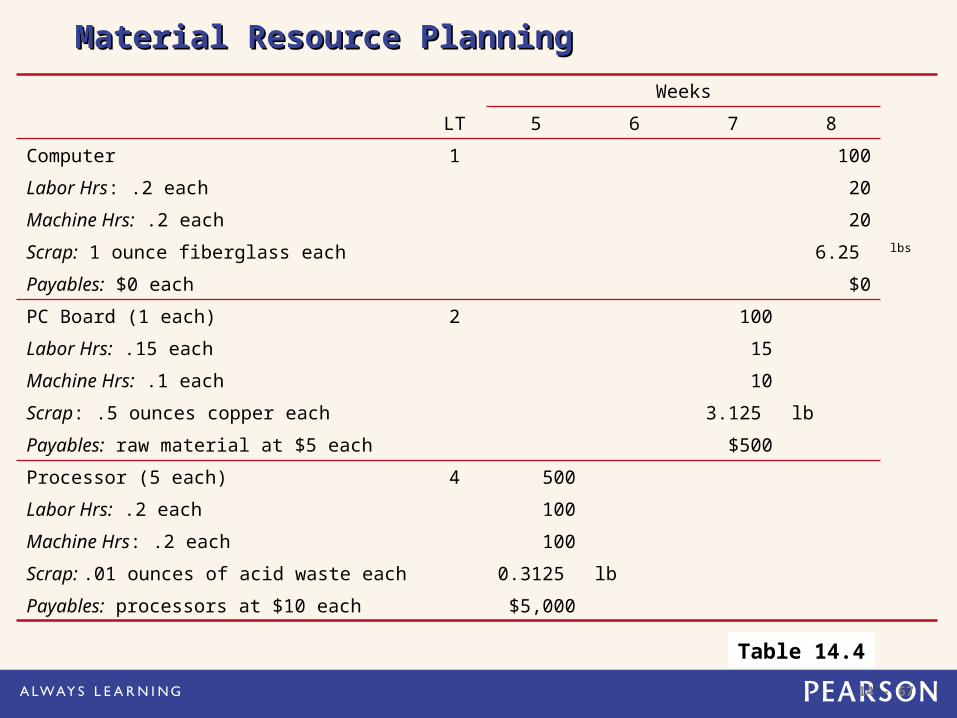
Material Requirements Planning IIMaterial Requirements Planning II
Requirement data can be enriched by other resources
Generally called MRP II or Material Resource Planning
Outputs include Scrap Packaging waste Carbon emissions
Data used by purchasing, production scheduling, capacity planning, inventory
14 - 67
Material Resource PlanningMaterial Resource PlanningWeeks
LT 5 6 7 8Computer 1 100Labor Hrs: .2 each 20Machine Hrs: .2 each 20Scrap: 1 ounce fiberglass each 6.25 lbs
Payables: $0 each $0PC Board (1 each) 2 100Labor Hrs: .15 each 15Machine Hrs: .1 each 10Scrap: .5 ounces copper each 3.125 lbPayables: raw material at $5 each $500Processor (5 each) 4 500Labor Hrs: .2 each 100Machine Hrs: .2 each 100Scrap: .01 ounces of acid waste each 0.3125 lbPayables: processors at $10 each $5,000
Table 14.4
14 - 68
Closed-Loop MRP SystemClosed-Loop MRP System
Figure 14.9
Priority Management
Develop Master ProductionSchedule
Prepare MaterialsRequirements Pan
Detailed ProductionActivity Control
(Shop Scheduling/Dispatching)
Capacity Management
Evaluate Resource Availability(Rough Cut)
Determine Capacity Availability
Implement Input/Output Control
Aggregate Production Plan
OK?OK?NONO
OK?OK?NONO OK? YESOK? YES
OK? YESOK? YES
Planning
Execution(in repetitive systems JIT techniques are used)
14 - 69
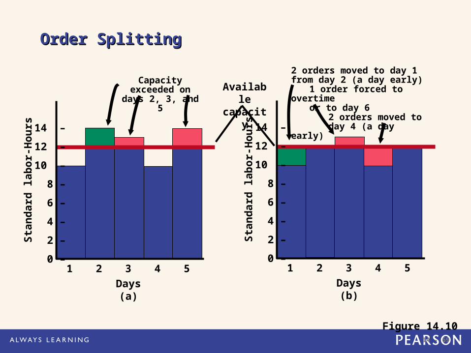
Order SplittingOrder Splitting
Figure 14.10
Available capacity
Capacity exceeded on days 2, 3, and 5
2 orders moved to day 1 from day 2 (a day early)
1 order forced to overtimeor to day 6
2 orders moved to day 4 (a day early)
14 –
12 –
10 –
8 –
6 –
4 –
2 –
0 –1 2 3 4 5
Days(b)
Stan
dard
labo
r-H
ours14 –
12 –
10 –
8 –
6 –
4 –
2 –
0 –1 2 3 4 5
Days(a)
Stan
dard
labo
r-H
ours
14 - 70
Capacity PlanningCapacity Planning
• Feedback from the MRP system
• Load reports show resource requirements for work centers
• Work can be moved between work centers to smooth the load or bring it within capacity
14 - 71
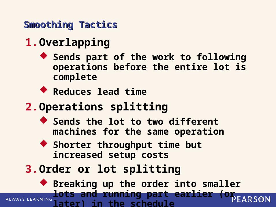
Smoothing TacticsSmoothing Tactics
1. Overlapping Sends part of the work to following
operations before the entire lot is complete Reduces lead time
2. Operations splitting Sends the lot to two different machines for
the same operation Shorter throughput time but increased setup
costs3. Order or lot splitting
Breaking up the order into smaller lots and running part earlier (or later) in the schedule
14 - 72
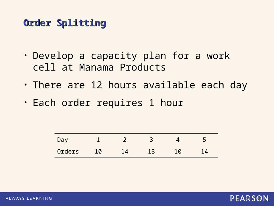
Order SplittingOrder Splitting
• Develop a capacity plan for a work cell at Manama Products
• There are 12 hours available each day
• Each order requires 1 hour
Day 1 2 3 4 5Orders 10 14 13 10 14
14 - 73
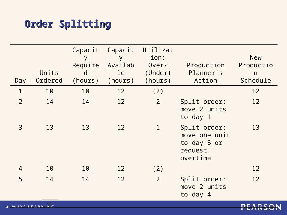
Order SplittingOrder Splitting
DayUnits
Ordered
Capacity Required (hours)
Capacity Available (hours)
Utilization: Over/
(Under) (hours)
Production Planner’s Action
New Production Schedule
1 10 10 12 (2) 12
2 14 14 12 2 Split order: move 2 units to day 1
12
3 13 13 12 1 Split order: move one unit to day 6 or request overtime
13
4 10 10 12 (2) 12
5 14 14 12 2 Split order: move 2 units to day 4
12
61
14 - 74
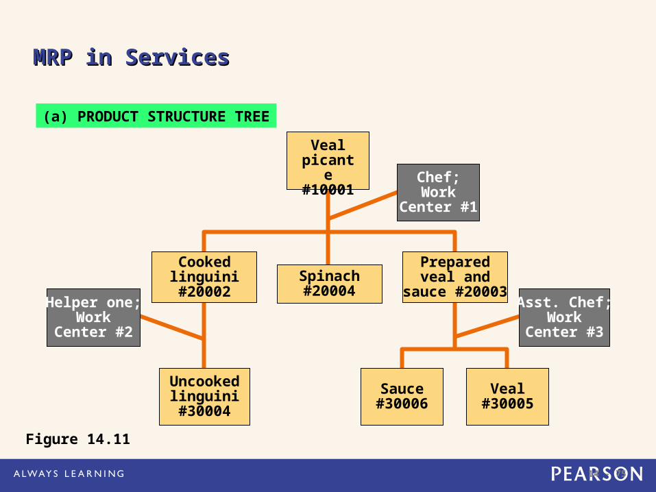
MRP in ServicesMRP in Services
Some services or service items are directly linked to demand for other services
These can be treated as dependent demand services or items Restaurants Hospitals Hotels
14 - 75
Uncooked linguini #30004
Sauce #30006
Veal #30005
MRP in ServicesMRP in Services
Chef;Work
Center #1
Helper one;Work
Center #2
Asst. Chef;Work
Center #3
Cooked linguini #20002
Spinach #20004
Prepared veal and sauce
#20003
(a) PRODUCT STRUCTURE TREE
Veal picante #10001
Figure 14.11
14 - 76
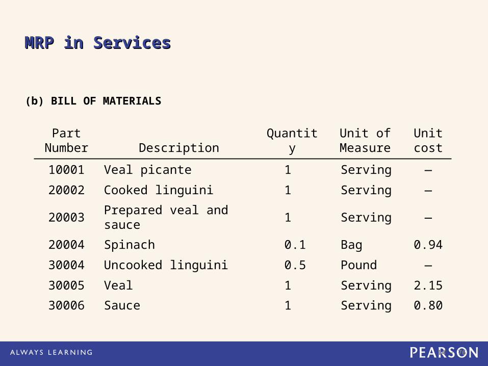
MRP in ServicesMRP in Services
(b) BILL OF MATERIALS
Part Number Description Quantity
Unit of Measure
Unit cost
10001 Veal picante 1 Serving —20002 Cooked linguini 1 Serving —
20003 Prepared veal and sauce 1 Serving —
20004 Spinach 0.1 Bag 0.9430004 Uncooked linguini 0.5 Pound —30005 Veal 1 Serving 2.1530006 Sauce 1 Serving 0.80
14 - 77
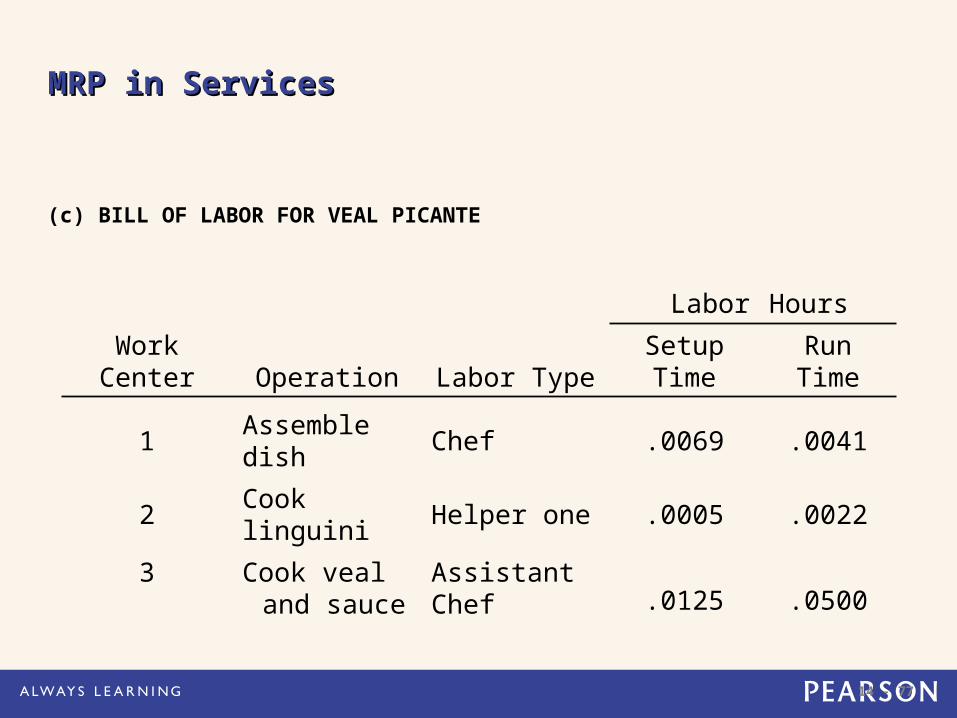
MRP in ServicesMRP in Services
(c) BILL OF LABOR FOR VEAL PICANTE
Labor HoursWork
Center Operation Labor TypeSetup Time
Run Time
1 Assemble dish Chef .0069 .0041
2 Cook linguini Helper one .0005 .0022
3 Cook veal and sauce
Assistant Chef .0125 .0500
14 - 78
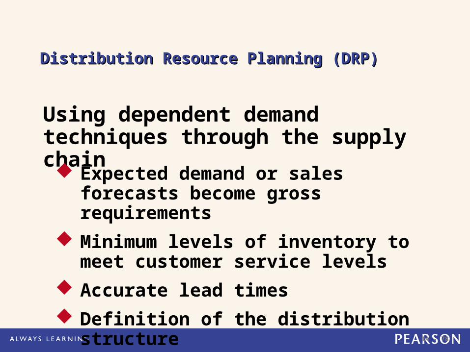
Distribution Resource Planning (DRP)Distribution Resource Planning (DRP)
Using dependent demand techniques through the supply chain Expected demand or sales forecasts
become gross requirements Minimum levels of inventory to meet
customer service levels Accurate lead times Definition of the distribution structure
14 - 79
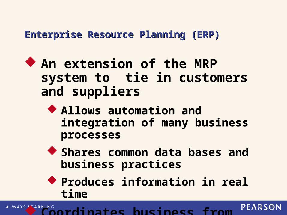
Enterprise Resource Planning (ERP)Enterprise Resource Planning (ERP)
An extension of the MRP system to tie in customers and suppliers Allows automation and integration of
many business processes Shares common data bases and
business practices Produces information in real time
Coordinates business from supplier evaluation to customer invoicing
14 - 80
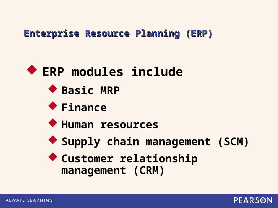
Enterprise Resource Planning (ERP)Enterprise Resource Planning (ERP)
ERP modules include Basic MRP Finance Human resources Supply chain management (SCM) Customer relationship management
(CRM)
14 - 81
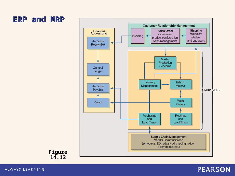
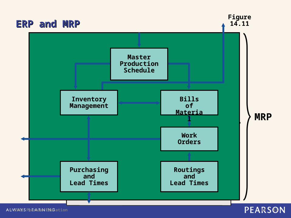
ERP and MRPERP and MRP
Figure 14.12
14 - 82
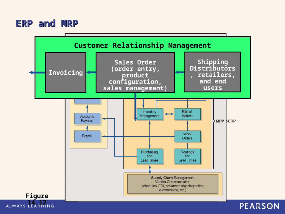
ERP and MRPERP and MRP
Figure 14.12
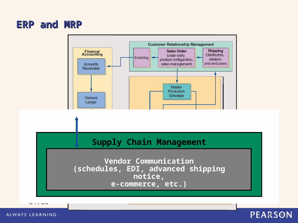
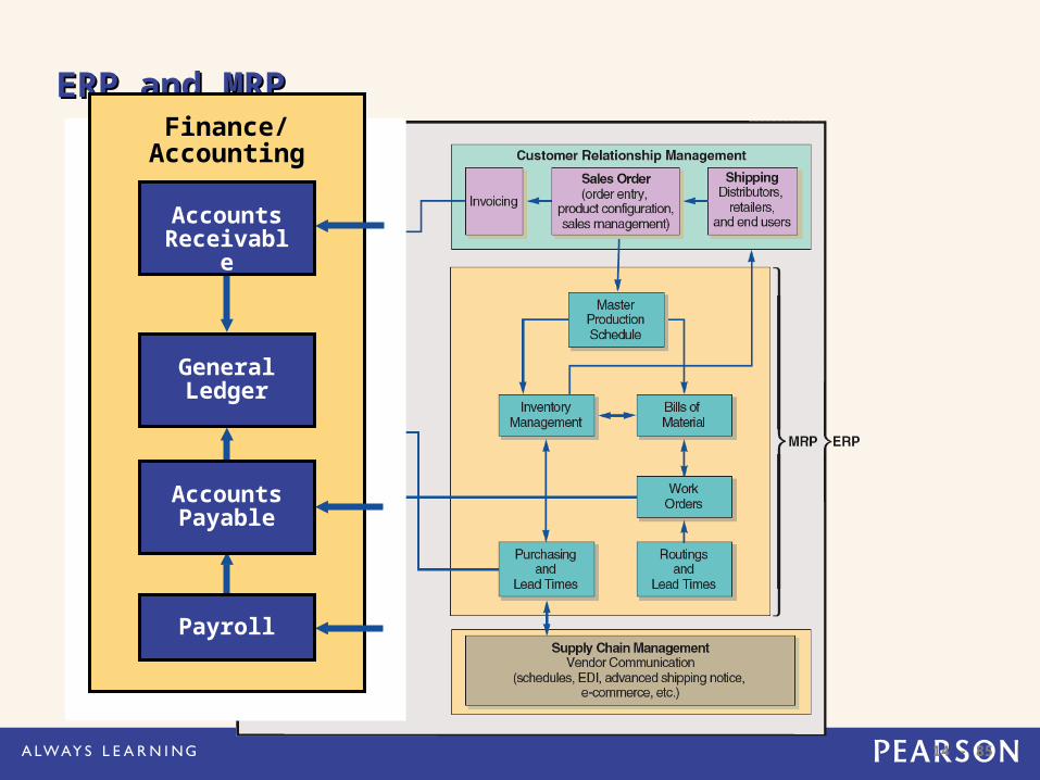
Customer Relationship Management
InvoicingShipping
Distributors, retailers,
and end users
Sales Order(order entry,
product configuration,sales management)
14 - 83© 2011 Pearson Education
Table 13.6
Bills of Material
Work Orders
Purchasingand
Lead Times
Routingsand
Lead Times
Master Production Schedule
Inventory Management
ERP and MRPERP and MRPFigure 14.11
MRP
14 - 84
ERP and MRPERP and MRP
Figure 14.11
Supply Chain Management
Vendor Communication(schedules, EDI, advanced shipping notice,
e-commerce, etc.)
14 - 85
ERP and MRPERP and MRP
Figure 14.11Table 13.6
Finance/Accounting
General Ledger
Accounts Receivable
Payroll
Accounts Payable
14 - 86
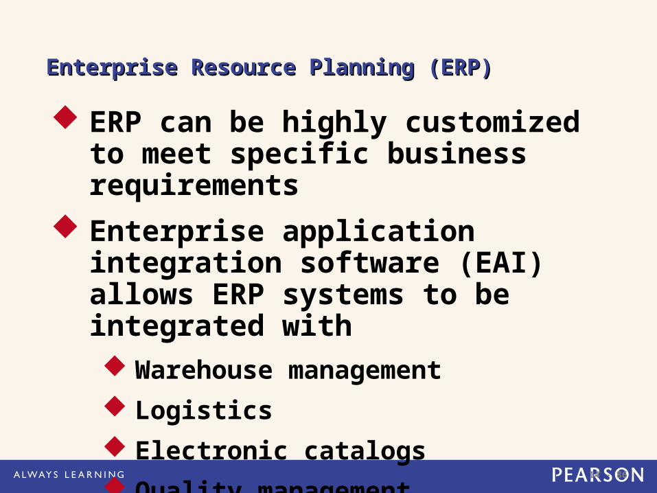
Enterprise Resource Planning (ERP)Enterprise Resource Planning (ERP)
ERP can be highly customized to meet specific business requirements
Enterprise application integration software (EAI) allows ERP systems to be integrated with Warehouse management Logistics Electronic catalogs Quality management
14 - 87
Enterprise Resource Planning (ERP)Enterprise Resource Planning (ERP)
ERP systems have the potential to Reduce transaction costs Increase the speed and accuracy of
information Facilitates a strategic emphasis on
JIT systems and integration
14 - 88
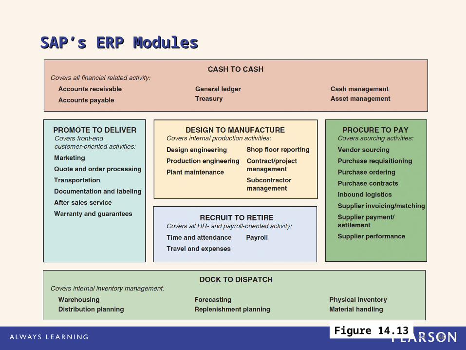
SAP’s ERP ModulesSAP’s ERP Modules
Figure 14.13
14 - 89
Advantages of ERP SystemsAdvantages of ERP Systems
1. Provides integration of the supply chain, production, and administration
2. Creates commonality of databases3. Can incorporate improved best processes4. Increases communication and
collaboration between business units and sites
5. Has an off-the-shelf software database6. May provide a strategic advantage
14 - 90
Disadvantages of ERP SystemsDisadvantages of ERP Systems
1. Is very expensive to purchase and even more so to customize
2. Implementation may require major changes in the company and its processes
3. Is so complex that many companies cannot adjust to it
4. Involves an ongoing, possibly never completed, process for implementation
5. Expertise is limited with ongoing staffing problems
14 - 91
ERP in the Service SectorERP in the Service Sector
ERP systems have been developed for health care, government, retail stores, hotels, and financial services
Also called efficient consumer response (ECR) systems
Objective is to tie sales to buying, inventory, logistics, and production