TitleHolographic Entanglement Entropy in the dS/CFTCorrespondence and Entanglement Entropy in the Sp(N)Model( Dissertation_全文 )

Author(s) Sato, Yoshiki

Citation Kyoto University (京都大学)

Issue Date 2016-03-23

URL https://doi.org/10.14989/doctor.k19494

Right

Type Thesis or Dissertation

Textversion ETD

Kyoto University

Holographic Entanglement Entropy in the

dS/CFT Correspondence and Entanglement

Entropy in the Sp(N) Model

Yoshiki Sato1

Department of Physics, Kyoto University

Kyoto 606-8502, Japan

Ph. D. Thesis

1E-mail: yoshiki@gauge.scphys.kyoto-u.ac.jp

Abstract

The AdS/CFT correspondence has been getting understood and we are now in a

position to explore gravitational theory by using conformal field theory by recent

progress on the holographic entanglement entropy. Nevertheless, the dS/CFT cor-

respondence, which has a possibility to describe our Universe holographically, is still

unclear.

We investigate the entanglement entropy in the dS/CFT correspondence. In

Einstein gravity on de Sitter spacetime we propose the holographic entanglement

entropy as the analytic continuation of the extremal surface in Euclidean anti-de

Sitter spacetime. Even though dual conformal field theories for Einstein gravity on

de Sitter spacetime are not known yet, we analyze the free Sp(N) model, which is

holographically dual to Vasiliev’s higher-spin gauge theory on de Sitter spacetime,

as a toy model. In this model we confirm the behaviour similar to our holographic

result from Einstein gravity.

This Ph. D. thesis is based on the papers [1, 2].

Acknowledgments

I would like to people who helped me during my master course and Ph. D. course.

Firstly, I would like to thank Prof. Kentaroh Yoshida in Department of Physics,

Kyoto university. He is one of my collaborators and my effective supervisor during

master and Ph. D. course. He has taught me a cutting edge of Physics such as

the AdS/CFT correspondence and how to write papers via collaborations about a

holographic Schwinger effect [3–8], carefully.

Next, I would like to thank Prof. Tadashi Takayanagi in Yukawa institute for

theoretical physics, Kyoto university. He guided me the holographic entanglement

entropy and a concerning topic. Discussions with him was very useful to carry out

my work [1] and his appropriate comments on the draft version of [1] made my paper

better.

I would like to thank Prof. Hikaru Kawai in Department of Physics, Kyoto

university. He is my supervisor during Ph. D. course and helped me many times.

His advise was just appropriate and I learned how to clearly present a research plan.

I would like to thank Prof. Hideo Suganuma in Department of Physics, Kyoto

university. He is an associate professor in nuclear theory group and a specialist on

quantum chromodynamics. Discussions with him were useful to finish the work of

the holographic Schwinger effect and to write a research plan for JSPS fellowship.

I also thank Dr. Yuhma Asano, Dr. Daisuke Kawai, Dr. Kiyoharu Kawana, Dr.

Hideki Kyono, Dr. Tomoki Nosaka, Dr. Masahiro Nozaki, Dr. Jun-ichi Sakamoto,

Dr. Noburo Shiba, and Dr. Kento Watanabe for useful discussions. Especially, I

would like to thank Dr. Tomoki Nosaka. He read the draft version of my paper [1]

and gave me many useful comments.

Finally, I would like to thank the members of Theoretical Particle Physics Group

at Dept. of Physics, Kyoto University.

During second and third degrees in Ph. D. course, I have been supported by

a Grant-in-Aid for Japan Society for the Promotion of Science (JSPS) Fellows

No.26·1300.

Publication List

This Ph. D. thesis is based on the following papers,

1. Y. Sato, “Comments on entanglement entropy in the dS/CFT correspon-

dence,” Phys. Rev. D 91 (2015) 8, 086009 [arXiv:1501.04903 [hep-th]].

2. Y. Sato, work in progress.

During my master and Ph. D. course, I published the other papers and the review

article [3–8] concerned with the holographic description of the Schwinger effect. This

Ph. D. thesis is not based on those paper [3–8].

1. Y. Sato and K. Yoshida, “Holographic description of the Schwinger effect in

electric and magnetic fields,” JHEP 1304 (2013) 111 [arXiv:1303.0112 [hep-

th]].

2. Y. Sato and K. Yoshida, “Potential Analysis in Holographic Schwinger Effect,”

JHEP 1308 (2013) 002 [arXiv:1304.7917 [hep-th]].

3. Y. Sato and K. Yoshida, “Holographic Schwinger effect in confining phase,”

JHEP 1309 (2013) 134 [arXiv:1306.5512 [hep-th]].

4. Y. Sato and K. Yoshida, “Universal aspects of holographic Schwinger effect in

general backgrounds,” JHEP 1312 (2013) 051 [arXiv:1309.4629 [hep-th]].

5. D. Kawai, Y. Sato and K. Yoshida, “Schwinger pair production rate in confin-

ing theories via holography,” Phys. Rev. D 89 (2014) 10, 101901 [arXiv:1312.4341

[hep-th]].

6. D. Kawai, Y. Sato and K. Yoshida, “A holographic description of the Schwinger

effect in a confining gauge theory,” Int. J. Mod. Phys. A 30 (2015) 11, 1530026

[arXiv:1504.00459 [hep-th]].

Contents

1 Introduction 3

2 Holography 8

2.1 AdS/CFT correspondence . . . . . . . . . . . . . . . . . . . . . . . . 8

2.1.1 Anti de Sitter spacetime . . . . . . . . . . . . . . . . . . . . . 8

2.1.2 Derivation of the AdS/CFT correspondence from string theory 10

2.2 dS/CFT correspondence . . . . . . . . . . . . . . . . . . . . . . . . . 14

2.2.1 de Sitter spacetime . . . . . . . . . . . . . . . . . . . . . . . . 14

2.2.2 dS/CFT correspondence . . . . . . . . . . . . . . . . . . . . . 16

2.2.3 Concrete example of the dS/CFT correspondence . . . . . . . 23

3 Entanglement Entropy and its Holographic Dual 25

3.1 Entanglement entropy . . . . . . . . . . . . . . . . . . . . . . . . . . 25

3.1.1 Definition . . . . . . . . . . . . . . . . . . . . . . . . . . . . . 25

3.1.2 Replica method . . . . . . . . . . . . . . . . . . . . . . . . . . 27

3.2 Holographic entanglement entropy . . . . . . . . . . . . . . . . . . . . 33

3.3 Proof of the Ryu-Takayanagi formula . . . . . . . . . . . . . . . . . . 36

4 Holographic Entanglement Entropy in Einstein Gravity on dS 41

4.1 Proposal . . . . . . . . . . . . . . . . . . . . . . . . . . . . . . . . . . 41

4.2 Extremal surfaces in asymptotically dS spacetime . . . . . . . . . . . 46

5 Entanglement Entropy in the Sp(N) Model 48

5.1 Sp(N) model . . . . . . . . . . . . . . . . . . . . . . . . . . . . . . . 48

5.2 Entanglement entropy . . . . . . . . . . . . . . . . . . . . . . . . . . 51

1

5.3 Comparison with A Toy CFT Model . . . . . . . . . . . . . . . . . . 54

6 Conclusion and Discussion 56

A Brown-York stress tensor 59

B Ricci scalar with a conical singularity 60

2

Chapter 1

Introduction

It is known that black holes (BH) have thermodynamic properties [9–11]. A BH

entropy is proportional to the horizon area,

SBH =Area of horizon

4GN

, (1.0.1)

where GN is Newton’s constant. Entropy represents degree of freedom of the sys-

tem and is typically proportional to a volume of the system. Nevertheless, the BH

entropy shows the area law not the volume law. This fact suggests that gravita-

tional theories can be described by lower dimensional field theories. This is called a

holographic principle [12, 13].

The AdS/CFT correspondence is a concrete realization of the holographic prin-

ciple [14–16]. It provides a remarkable connection between gravitational theories in

anti-de Sitter spacetime (AdS) and nongravitational conformal field theories (CFT).

A validity of the AdS/CFT correspondence has been checked only in the region that

the gravitational theories can be approximated by classical gravitational theories.

Despite of this limitation, the holographic principle, especially the AdS/CFT cor-

respondence, provides us to analyze quantum gravitational theories by using non-

gravitational theories.

A useful quantity to analyze gravitational theories in the context of the AdS/CFT

correspondence, is the holographic entanglement entropy proposed by Ryu and

3

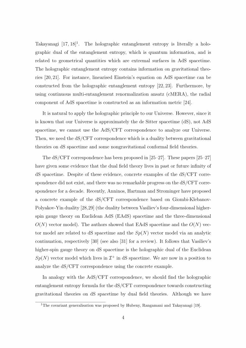
Takayanagi [17, 18]1. The holographic entanglement entropy is literally a holo-

graphic dual of the entanglement entropy, which is quantum information, and is

related to geometrical quantities which are extremal surfaces in AdS spacetime.

The holographic entanglement entropy contains information on gravitational theo-

ries [20, 21]. For instance, linearised Einstein’s equation on AdS spacetime can be

constructed from the holographic entanglement entropy [22, 23]. Furthermore, by

using continuous multi-entanglement renormalization ansatz (cMERA), the radial

component of AdS spacetime is constructed as an information metric [24].

It is natural to apply the holographic principle to our Universe. However, since it

is known that our Universe is approximately the de Sitter spacetime (dS), not AdS

spacetime, we cannot use the AdS/CFT correspondence to analyze our Universe.

Then, we need the dS/CFT correspondence which is a duality between gravitational

theories on dS spacetime and some nongravitational conformal field theories.

The dS/CFT correspondence has been proposed in [25–27]. These papers [25–27]

have given some evidence that the dual field theory lives in past or future infinity of

dS spacetime. Despite of these evidence, concrete examples of the dS/CFT corre-

spondence did not exist, and there was no remarkable progress on the dS/CFT corre-

spondence for a decade. Recently, Anninos, Hartman and Strominger have proposed

a concrete example of the dS/CFT correspondence based on Giombi-Klebanov-

Polyakov-Yin duality [28,29] (the duality between Vasiliev’s four-dimensional higher-

spin gauge theory on Euclidean AdS (EAdS) spacetime and the three-dimensional

O(N) vector model). The authors showed that EAdS spacetime and the O(N) vec-

tor model are related to dS spacetime and the Sp(N) vector model via an analytic

continuation, respectively [30] (see also [31] for a review). It follows that Vasiliev’s

higher-spin gauge theory on dS spacetime is the holographic dual of the Euclidean

Sp(N) vector model which lives in I+ in dS spacetime. We are now in a position to

analyze the dS/CFT correspondence using the concrete example.

In analogy with the AdS/CFT correspondence, we should find the holographic

entanglement entropy formula for the dS/CFT correspondence towards constructing

gravitational theories on dS spacetime by dual field theories. Although we have

1The covariant generalisation was proposed by Hubeny, Rangamani and Takayanagi [19].

4

the concrete example of the dS/CFT correspondence, Vasiliev’s higher-spin gauge

theory contains infinite massless particles and is not suitable for a description of our

Universe. Furthermore, it is difficult to analyze Vasiliev’s higher-spin gauge theory

since an equation of motion is only known but a satisfactory action is not known

yet.

In this Ph. D. thesis, we summarize our papers [1,2] which discuss the holographic

entanglement entropy in the dS/CFT correspondence and the entanglement entropy

in the Sp(N) model. In [1], we investigate the connection between bulk geometry and

the holographic entanglement entropy in Einstein gravity on dS spacetime not the

Vasiliev’s higher-spin gauge theory on dS spacetime. We also compare the proposed

holographic entanglement entropy with the entanglement entropy in the free Sp(N)

model, which is the holographic dual of Vasiliev’s higher-spin gauge theory on dS

spacetime. Furthermore, we investigate the detail of the entanglement entropy in

the Sp(N) model in [2].

Outline

The organization of this Ph. D. thesis is as follows.

Chapter 2 and 3 are devoted to preliminaries of chapter 4 and chapter 5. In

chapter 2 we review the AdS/CFT correspondence and the dS/CFT correspondence.

In section 2.1, we will give a definition of AdS spacetime, a heuristic derivation of the

AdS/CFT correspondence, and a useful relation in the AdS/CFT correspondence,

GKPW relation. Then, we move to the dS/CFT correspondence in section 2.2.

Firstly, we define dS geometry. Next, we explain difficulties to construct the dS/CFT

correspondence and summarize fundamental works of the dS/CFT correspondence.

In chapter 3 we will explain a notion of the entanglement entropy in quantum field

theory. Also, the holographic dual of the entanglement entropy will be introduced.

We will give a proof of the Ryu-Takayanagi formula and explain that the holographic

entanglement entropy is regarded as a generalised quantity of the BH entropy.

Chapter 4 and 5 are a summary of the paper [1] and the work in progress [2].

In chapter 4 we give a proposal for the holographic entanglement entropy formula

for Einstein gravity on dS spacetime based on the paper [1]. We find extremal

5

surfaces in Poincare dS coordinate by using a double Wick rotation from EAdS in

Poincare coordinates. We also comment on extremal surfaces in more general set of

asymptotically dS spacetime. In chapter 5 we calculate the entanglement entropy

in the free Euclidean Sp(N) model. We compare the entanglement entropy in the

Sp(N) model with the proposed holographic entanglement entropy in chapter 4 and

confirm that our proposal is sensible qualitatively. We also study the entanglement

entropy in the Sp(N) model in more detail. Chapter 6 is devoted to a conclusion

and discussion.

6

Notation

We summarize our notations, here.

Dimension

Gravitational theories are defined on (d+1)-dimensional spacetime, while dual field

theories are defined on d-dimensional spacetime.

Index

We use indices M,N, · · · for (d+ 1)-dimensional spacetime and indices µ, ν, · · · ford-dimensional spacetime.

7

Chapter 2

Holography

In this chapter, we give an overview of the AdS/CFT correspondence, firstly. Then,

we will review the proposed dS/CFT correspondence and some related works.

2.1 AdS/CFT correspondence

2.1.1 Anti de Sitter spacetime

Before explanations of the AdS/CFT correspondence, we summarize AdS geometry.

(d + 1)-dimensional anti-de Sitter spacetime (AdS) is defined as a hypersurface

in Minkowski spacetime (X0, · · · , Xd+1) satisfying the relation

−X20 +X2

1 + · · ·+X2d −X2

d+1 = ℓ2AdS , (2.1.1)

where ℓAdS is an AdS radius. When we take a time-direction Euclidean, the geometry

becomes a hyperbolic space Hd+1. The hyperbolic space is also called Euclidean AdS

spacetime (EAdS). The metric of AdS spacetime is introduced by

ds2 = − dX20 + dX2

1 + · · ·+ dX2d − dX2

d+1 . (2.1.2)

Naively, it seems that the metric (2.1.2) contains two time-directions. Nevertheless

we will see that the metric (2.1.2) contains only one time-direction in the following

discussion.

8

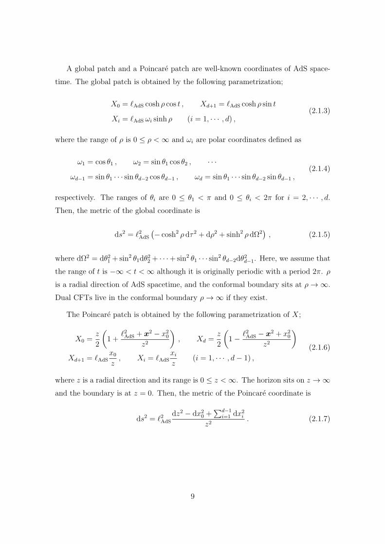
A global patch and a Poincare patch are well-known coordinates of AdS space-

time. The global patch is obtained by the following parametrization;

X0 = ℓAdS cosh ρ cos t , Xd+1 = ℓAdS cosh ρ sin t

Xi = ℓAdS ωi sinh ρ (i = 1, · · · , d) ,(2.1.3)

where the range of ρ is 0 ≤ ρ <∞ and ωi are polar coordinates defined as

ω1 = cos θ1 , ω2 = sin θ1 cos θ2 , · · ·

ωd−1 = sin θ1 · · · sin θd−2 cos θd−1 , ωd = sin θ1 · · · sin θd−2 sin θd−1 ,(2.1.4)

respectively. The ranges of θi are 0 ≤ θ1 < π and 0 ≤ θi < 2π for i = 2, · · · , d.Then, the metric of the global coordinate is

ds2 = ℓ2AdS

(− cosh2 ρ dτ 2 + dρ2 + sinh2 ρ dΩ2

), (2.1.5)

where dΩ2 = dθ21 + sin2 θ1dθ22 + · · ·+ sin2 θ1 · · · sin2 θd−2dθ

2d−1. Here, we assume that

the range of t is −∞ < t <∞ although it is originally periodic with a period 2π. ρ

is a radial direction of AdS spacetime, and the conformal boundary sits at ρ→∞.

Dual CFTs live in the conformal boundary ρ→∞ if they exist.

The Poincare patch is obtained by the following parametrization of X;

X0 =z

2

(1 +

ℓ2AdS + x2 − x20z2

), Xd =

z

2

(1− ℓ2AdS − x2 + x20

z2

)Xd+1 = ℓAdS

x0z, Xi = ℓAdS

xiz

(i = 1, · · · , d− 1) ,

(2.1.6)

where z is a radial direction and its range is 0 ≤ z <∞. The horizon sits on z →∞and the boundary is at z = 0. Then, the metric of the Poincare coordinate is

ds2 = ℓ2AdS

dz2 − dx20 +∑d−1

i=1 dx2i

z2. (2.1.7)

9

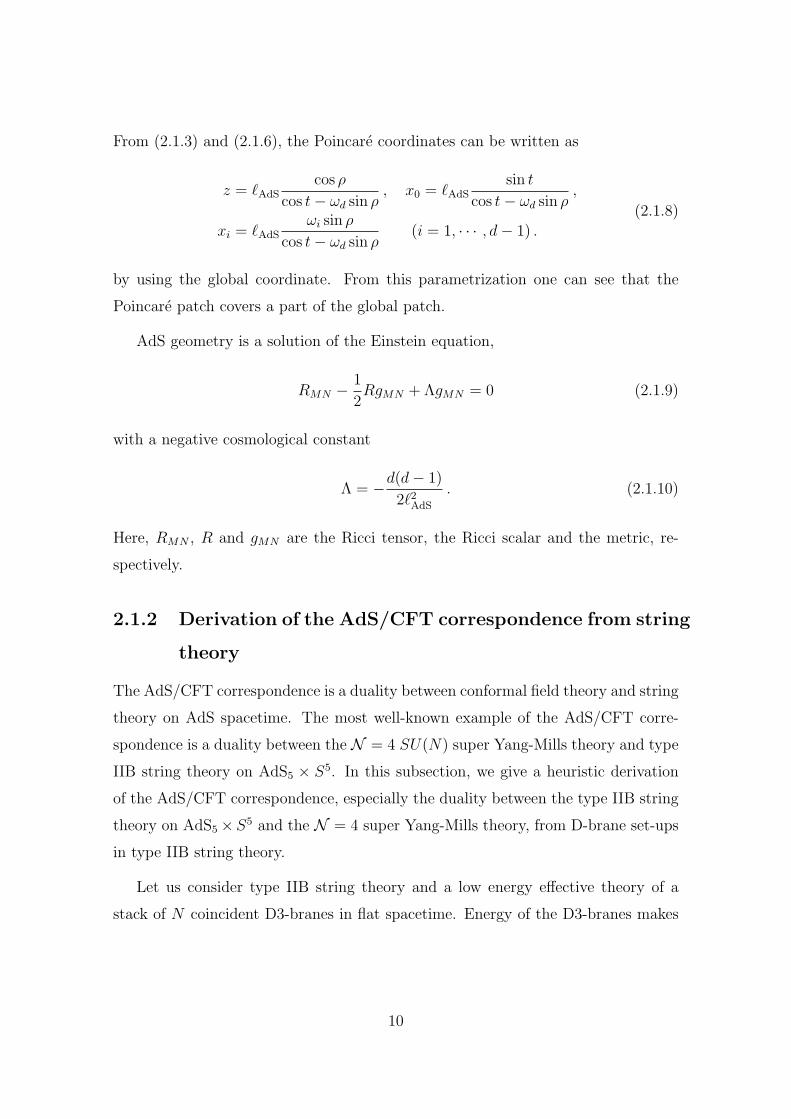
From (2.1.3) and (2.1.6), the Poincare coordinates can be written as

z = ℓAdScos ρ

cos t− ωd sin ρ, x0 = ℓAdS

sin t

cos t− ωd sin ρ,

xi = ℓAdSωi sin ρ

cos t− ωd sin ρ(i = 1, · · · , d− 1) .

(2.1.8)

by using the global coordinate. From this parametrization one can see that the

Poincare patch covers a part of the global patch.

AdS geometry is a solution of the Einstein equation,

RMN −1

2RgMN + ΛgMN = 0 (2.1.9)

with a negative cosmological constant

Λ = −d(d− 1)

2ℓ2AdS

. (2.1.10)

Here, RMN , R and gMN are the Ricci tensor, the Ricci scalar and the metric, re-

spectively.

2.1.2 Derivation of the AdS/CFT correspondence from string

theory

The AdS/CFT correspondence is a duality between conformal field theory and string

theory on AdS spacetime. The most well-known example of the AdS/CFT corre-

spondence is a duality between the N = 4 SU(N) super Yang-Mills theory and type

IIB string theory on AdS5 × S5. In this subsection, we give a heuristic derivation

of the AdS/CFT correspondence, especially the duality between the type IIB string

theory on AdS5×S5 and the N = 4 super Yang-Mills theory, from D-brane set-ups

in type IIB string theory.

Let us consider type IIB string theory and a low energy effective theory of a

stack of N coincident D3-branes in flat spacetime. Energy of the D3-branes makes

10

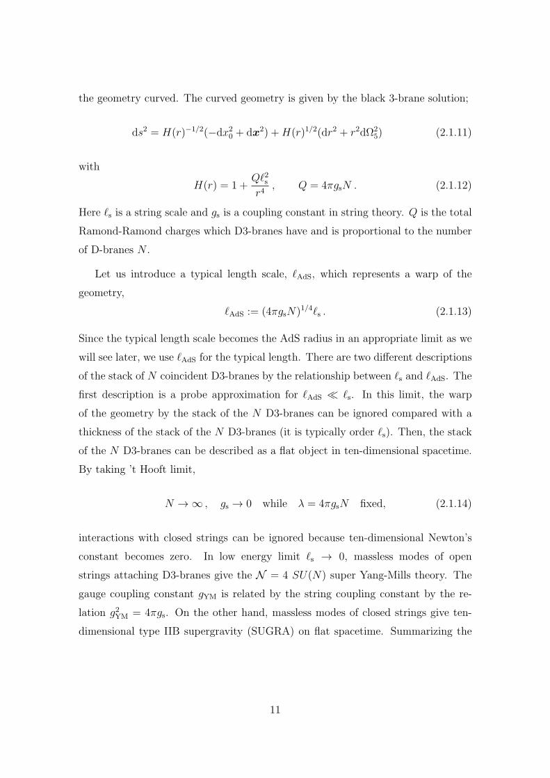
the geometry curved. The curved geometry is given by the black 3-brane solution;

ds2 = H(r)−1/2(−dx20 + dx2) +H(r)1/2(dr2 + r2dΩ25) (2.1.11)

with

H(r) = 1 +Qℓ2sr4

, Q = 4πgsN . (2.1.12)

Here ℓs is a string scale and gs is a coupling constant in string theory. Q is the total

Ramond-Ramond charges which D3-branes have and is proportional to the number

of D-branes N .

Let us introduce a typical length scale, ℓAdS, which represents a warp of the

geometry,

ℓAdS := (4πgsN)1/4ℓs . (2.1.13)

Since the typical length scale becomes the AdS radius in an appropriate limit as we

will see later, we use ℓAdS for the typical length. There are two different descriptions

of the stack of N coincident D3-branes by the relationship between ℓs and ℓAdS. The

first description is a probe approximation for ℓAdS ≪ ℓs. In this limit, the warp

of the geometry by the stack of the N D3-branes can be ignored compared with a

thickness of the stack of the N D3-branes (it is typically order ℓs). Then, the stack

of the N D3-branes can be described as a flat object in ten-dimensional spacetime.

By taking ’t Hooft limit,

N →∞ , gs → 0 while λ = 4πgsN fixed, (2.1.14)

interactions with closed strings can be ignored because ten-dimensional Newton’s

constant becomes zero. In low energy limit ℓs → 0, massless modes of open

strings attaching D3-branes give the N = 4 SU(N) super Yang-Mills theory. The

gauge coupling constant gYM is related by the string coupling constant by the re-

lation g2YM = 4πgs. On the other hand, massless modes of closed strings give ten-

dimensional type IIB supergravity (SUGRA) on flat spacetime. Summarizing the

11

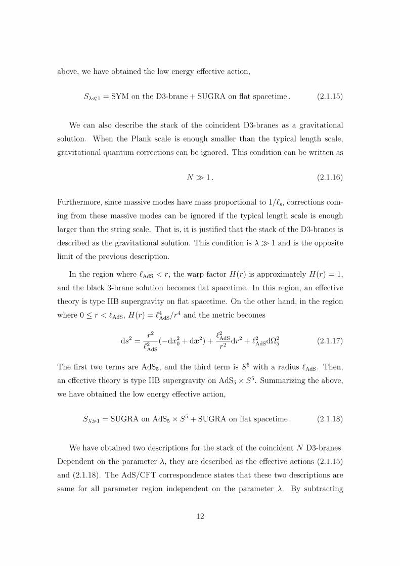
above, we have obtained the low energy effective action,

Sλ≪1 = SYM on the D3-brane + SUGRA on flat spacetime . (2.1.15)

We can also describe the stack of the coincident D3-branes as a gravitational

solution. When the Plank scale is enough smaller than the typical length scale,

gravitational quantum corrections can be ignored. This condition can be written as

N ≫ 1 . (2.1.16)

Furthermore, since massive modes have mass proportional to 1/ℓs, corrections com-

ing from these massive modes can be ignored if the typical length scale is enough

larger than the string scale. That is, it is justified that the stack of the D3-branes is

described as the gravitational solution. This condition is λ≫ 1 and is the opposite

limit of the previous description.

In the region where ℓAdS < r, the warp factor H(r) is approximately H(r) = 1,

and the black 3-brane solution becomes flat spacetime. In this region, an effective

theory is type IIB supergravity on flat spacetime. On the other hand, in the region

where 0 ≤ r < ℓAdS, H(r) = ℓ4AdS/r4 and the metric becomes

ds2 =r2

ℓ2AdS

(−dx20 + dx2) +ℓ2AdS

r2dr2 + ℓ2AdSdΩ

25 (2.1.17)

The first two terms are AdS5, and the third term is S5 with a radius ℓAdS. Then,

an effective theory is type IIB supergravity on AdS5 × S5. Summarizing the above,

we have obtained the low energy effective action,

Sλ≫1 = SUGRA on AdS5 × S5 + SUGRA on flat spacetime . (2.1.18)

We have obtained two descriptions for the stack of the coincident N D3-branes.

Dependent on the parameter λ, they are described as the effective actions (2.1.15)

and (2.1.18). The AdS/CFT correspondence states that these two descriptions are

same for all parameter region independent on the parameter λ. By subtracting

12

“type IIB supergravity on flat spacetime,” it means that the four-dimensionalN = 4

SU(N) super Yang-Mills theory is equivalent to type IIB string theory on AdS5×S5

for arbitrary λ. The AdS/CFT correspondence is a merely conjecture, and there

is no rigorous proof. Nevertheless, if we believe that the AdS/CFT description is

valid for all parameter regions N and λ, we can regard that gauge theory defines

“quantum” gravitational theory via the AdS/CFT correspondence. Therefore, the

AdS/CFT correspondence is very fascinating.

From now on we take ’t Hooft limit and λ→∞ limit unless otherwise noted.

GKPY relation

A useful relation in the AdS/CFT correspondence is the Gubser-Klebanov-Polyakov-

Witten (GKPW) relation [15, 16]. It gives us the fundamental principle which rep-

resents how physical quantities in both gravity side and gauge side are related. It

states that partition functions of both gravity side and gauge side are equivalent,

ZG[ϕi] =

⟨exp

(−∫ddxOiJi(x)

)⟩CFT

. (2.1.19)

(2.1.19) is the Euclidean version of the GKPW relation, and we will see its detail

from now on.

The left hand side in (2.1.19), ZG[ϕi], is the partition function of gravitational

theory. The subscript G in ZG means Gravity. ϕi represent all fields in the gravita-

tional theory and are proportional to the external fields Ji at the conformal bound-

ary. ZG[ϕi] is given by the path integral about ϕi with the boundary condition

ϕi ∝ Ji at the AdS boundary. In the case that the gravitational theory can be

approximated by the classical gravity, the partition function can be evaluated as

ZG[ϕi] = e−SG[ϕi] , (2.1.20)

where SG[ϕi] means the on-shell action with the boundary condition ϕi ∝ Ji at the

AdS boundary.

The right hand side in (2.1.19) is the expectation value in CFT. Oi are operators

in CFT, and Ji are external fields coupled to Oi. For instance, an energy-momentum

13

tensor Tµν in CFT couples to the metric gµν .

By using the GKPW relation, we can evaluate physical quantities at strong cou-

pling such as correlation functions. We can also evaluate thermodynamical quanti-

ties such as entropy. In subsection 3.3, we will see that the Ryu-Takayanagi conjec-

ture is derived via the GKPW relation (2.1.19).

2.2 dS/CFT correspondence

The dS/CFT correspondence are proposed dualities between gravitational theories

on dS spacetime and Euclidean conformal field theory on the future infinity I+.After we introduce dS geometry in the next subsection, problems to construct the

dS/CFT correspondence are introduced in subsection 2.2.2. And, we discuss funda-

mental works in the rest of subsection 2.2.2 and the higher-spin dS/CFT correspon-

dence in subsection 2.2.3.

2.2.1 de Sitter spacetime

(d+ 1)-dimensional de Sitter spacetime (dS) is defined as a hepersurface satisfying

the following relation,

−X20 +X2

1 + · · ·+X2d+1 = ℓ2dS , (2.2.1)

where ℓdS is a dS radius. dS satisfies the Einstein equation with a positive cosmo-

logical constant Λ = d(d− 1)/2ℓ2dS. A dS metric is introduced by

ds2 = − dX20 + dX2

1 + · · ·+ dX2d+1 . (2.2.2)

Next, we introduce a global patch and a Poincare patch of dS spacetime. Assume

that coordinates X are

X0 = ℓdS sinh τ , Xi = ℓdS ωi cosh τ (i = 1, · · · , d+ 1) , (2.2.3)

where −∞ < τ <∞ and ωi are polar coordinates introduced in (2.1.4). The metric

14

becomes

ds2 = ℓ2dS(−dτ 2 + cosh2 τ dΩ2) . (2.2.4)

This patch is called a global coordinate and covers a whole of dS spacetime. One can

see that the dS spacetime has no spatial boundaries in opposite to AdS spacetime or

flat spacetime. Nevertheless, dS spacetime has two boundaries, a future boundary

I+ and a past boundary I−.

Next we move to the Poincare patch. By substituting

X0 = −ℓdS(sinhT +

x2

2eT),

Xi = ℓdS xi eT (i = 1, · · · , d) ,

Xd+1 = ℓdS

(coshT − x2

2eT),

(2.2.5)

to (2.2.2), we obtain the Poincare patch of dS spacetime. The metric becomes

ds2 = ℓ2dS(− dT 2 + e2Tdx2) . (2.2.6)

Note that the Poincare patch covers only a half of dS spacetime. The future infinity

corresponds to T =∞. By introducing a conformal time,

η = eT , (2.2.7)

the metric of the Poincare patch of dS spacetime can be written as

ds2 = ℓ2dS−dη2 +

∑di=1 dx

2i

η2. (2.2.8)

By performing a double Wick rotation,

η → iz , ℓdS → iℓAdS , (2.2.9)

the metric (2.2.8) becomes the metric in the Poincare EAdS spacetime,

ds2 = ℓ2AdS

dz2 +∑d−1

i=0 dx2i

z2. (2.2.10)

15

2.2.2 dS/CFT correspondence

While the AdS/CFT correspondence has been well-studied, the dS/CFT correspon-

dence has been unclear even at the classical level. There are many problems to

construct the dS/CFT correspondence. Main problems are follows;

1. For holography to work, it seems that spatial boundaries are needed like AdS

spacetime. Since dS spacetime is topologically R × Sd and has no spatial

boundary, the holography might not work in dS spacetime, naively.

2. In analogy with the heuristic derivation of the AdS/CFT correspondence re-

viewed in subsection 2.1.2, we would like to derive the dS/CFT correspondence

form string theory. Nevertheless, it is impossible to construct dS spacetime as

solutions of supergravity [32]. Furthermore, α′ corrections are not useful to

resolve this problem [33]. That is, dS spacetime might not be constructed in

string theory.

3. dS spacetime can be obtained by the analytical continuation of AdS spacetime.

Then, it is expected that the dS/CFT correspondence might be obtained by

the analytical continuation of the AdS/CFT correspondence. Nevertheless,

we encounter imaginary fluxes or conformal weight, and ghosts fields in the

gravity, when we perform the analytical continuation of AdS solutions in string

theory. The analytical continuation is typically failed.

4. Analytical continuations of the AdS/CFT correspondence give non-unitary

CFT. This fact seems to contradict with unitarity of dS spacetime since CFTs

holographic dual to dS spacetime should have been unitary if the dS/CFT

correspondence has held.

The problem 1 is resolved by assuming that dual field theories live on the past or

future infinities. In fact, conformal field theories are assumed to live in I− or I+

in the proposed dS/CFT correspondence. The problem 2 suggests that we should

consider string theory without supersymmetry. There is no remarkable progress on

this point in the context of the dS/CFT correspondence. In terms of the problem

3, a remarkable progress occurred. A concrete example was found. Although the

16

analytical continuation of the AdS/CFT correspondence obtained from D-brane set-

ups is not appropriate, we can obtain examples of the dS/CFT correspondence by

the analytical continuation of higher-spin gauge theory. We will see a detail in

subsection 2.2.3. The problem 4 may be resolved by pseudo unitarity which field

theory holographic dual to dS has in general. Note however that there is a paper [34]

which states that the dS/CFT correspondence does not exist.

From now on, we will review some fundamental works in the dS/CFT correspon-

dence in the rest of subsection 2.2.2 and shows the concrete example of the dS/CFT

correspondence in subsection 2.2.3.

Asymptotic symmetries

Consider asymptotic symmetries of dS spacetime [26] (see [35] for a review), which

are defined as the group of allowed symmetries divided by the group of trivial sym-

metries. The allowed symmetries are symmetries which satisfy the boundary con-

dition we impose, and the trivial symmetries are symmetries which have vanishing

generators under constraints.

For simplicity, we consider a dS3 case. By introducing a complex coordinate

z = x1 + ix2 and its complex conjugate z = x − iy, the Poincare metric can be

written as

ds2 = ℓ2dS(−dτ 2 + e2τ dzdz) . (2.2.11)

We impose a boundary condition at I+ as

gzz =ℓ2dS2e2τ +O(1) , gττ = −ℓ2dS +O(e−2τ ) , gzz = gτz = O(1) . (2.2.12)

This boundary condition (2.2.12) is that in [35]. It is different from that in [26]

and an analytical continuations of the AdS boundary condition in [36]. We choose

the boundary condition (2.2.12) such that a perturbed Brown-York tensor should

be finite. Here the Brown-York tensor for dS3 is given by

Tµν =1

4GN

(Kµν −

(K +

1

ℓdS

)γµν

), (2.2.13)

17

where γµν is the induced metric on the future boundary I+ and Kµν is an extrinsic

curvature. See Appendix A for detail. The Brown-York tensor is zero for the planar

metric. For the perturbed metric gµν + hµν , the Brown-York tensor becomes

Tzz =1

4GN

(hzz − ∂zhτz +

1

2∂τhzz

),

Tzz =1

4GN

(hzz − ∂zhτz +

1

2∂τhzz

).

(2.2.14)

The most general diffeomorphism which preserves the boundary condition can

be written as

ζ = U∂z +1

2e−2τU ′′∂z −

1

2U ′∂τ +O(e−2τ ) + complex conjugate, (2.2.15)

where U = U(z) is a holomorphic function about z and the prime denote z-

derivative. In the following, we omit the anti-holomorphic part, for simplicity. The

reason that the most general diffeomorphism is (2.2.15) is that the Lie derivative of

the metric δζgµν = −Lζgµν = −(∇µζν +∇νζµ) = −(gµρ∂νζρ + gνρ∂µζρ + ζρ∂ρgµν)

1,

becomes

δζgzz = −ℓ2dS2U ′′′ , δζgττ = δζgzz = δζgzz = 0 , (2.2.16)

and the change of the metric preserves the boundary condition (2.2.12).

A special case is

U = α + βz + γz2 (2.2.17)

with complex constant parameters α, β, γ. In this case, U ′′′ vanishes. It means that

the metric is invariant under the diffeomorphism. Consider a commutation relation

between Lie derivatives with the vector fields ζ1 and ζ2, which have parameters U1

and U2, respectively. The commutation relation becomes

[Lζ1 ,Lζ2 ] = L[ζ1,ζ2] = Lζ3 (2.2.18)

where ζ3 is a vector field with parameter U3 = U1U′2 − U ′

1U2. The vector fields with

1 The Lie derivative of a rank two tensor Tµν is given by LζTµν = Tµρ∂νζρ+Tρν∂µζ

ρ+ζρ∂ρTµν .

18

parameters U = 1, U = 2z, and U = z2 satisfy commutation relations,

[ζU=1, ζU=1] = [ζU=2z, ζU=2z] = [ζU=z2 , ζU=z2 ] = 0 ,

[ζU=1, ζU=2z] = 2ζU=1 , [ζU=2z, ζU=z2 ] = 2ζU=z2 , [ζU=1, ζU=z2 ] = ζU=2z .(2.2.19)

This is an SL(2,C) algebra. In conclusion the diffeomorphism with the parameter

U = α + βz + γz2 generates the SL(2,C) isometry.

Next, we will find the central charge. The diffeomorphism acts on the perturba-

tive Brown-York tensor as

δζTzz = −U∂Tzz − 2U ′Tzz −ℓdS8GN

U ′′′ . (2.2.20)

Since the stress energy tensor T transforms as

δζT = − c

12U ′′′ − 2U ′T − U∂T , (2.2.21)

in general CFTs with the central charge c, we notice that the central charge is

c =3ℓdS2GN

. (2.2.22)

State/operator relation

The dS/CFT correspondence proposes that the wave function of a universe which is

asymptotically dS spacetime is evaluated by a partition function of Euclidean CFT,

Ψ[gij] = ZCFT[gij] . (2.2.23)

The left hand side is the wave function of a universe with a boundary metric gij,

and the right hand side is the partition function on the manifold with the metric

gij. We develop the state/operator relation from the discussion about propagator

below.

Consider propagators in dS3 [26], firstly. It is expected that propagators from

the future infinity to the future infinity in dS spacetime become those of the dual

19

CFT2. We will see this from now on.

The Klein-Gordon equation of a scalar field with mass m is given by

m2ℓ2dSϕ = ℓ2dS∇2ϕ = −∂2τϕ− 2∂τϕ+ 4e−2τ∂z∂zϕ . (2.2.24)

Since the last term can be negligible near the future infinity, solutions of the wave

equation behave as

ϕ(τ, z, z) ∼ e−h±τϕ±(z, z) , τ →∞ (2.2.25)

where h± are defined as

h± = 1±√1−m2ℓ2dS . (2.2.26)

We only consider the case where 0 < m2ℓ2dS < 13. In this case, h± are real and

satisfy the relation h− < 1 < h+. We impose the boundary condition on I+,

limτ→∞

ϕ(τ, z, z) = e−h−τϕ−(z, z) . (2.2.27)

In analogy with the AdS/CFT correspondence, the dS/CFT proposes that ϕ− is

holographic dual to an operator Oϕ with a conformal dimension h+ in the dual

CFT. The two-point function of Oϕ is proportional to the quadratic coefficient of

ϕ− in the on-shell action. If we perform the same calculation in the AdS/CFT

correspondence case, we can obtain the two-point function of Oϕ,

⟨Oϕ(z, z)Oϕ(v, v)⟩ =const.

|z − v|2h+. (2.2.28)

In conclusion, we reproduce the two-point function of Oϕ of h+ from the gravity

side. This is another evidence that the dual CFT lives on the future infinity. There

are similar works [37–39].

Next, we consider the two-point function, more precisely following by [27]. We

want to focus on the result and skip the detail discussion here. We consider four-

2In [26], propagators from the past infinity from the past infinity are considered. There is nochange in the discussion.

3In the case m2ℓ2dS > 1, h± become complex. This suggests that the dual CFT is non-unitary.

20

dimensional Pincare dS spacetime and assume that all fields start in the Bunch-

Davies vacuum. To begin with, calculate the wave function as a function of a

massless scalar field at a reference time ηc. We assume that the scaler field is small.

By substituting the classical solution in momentum space,

ϕ = ϕ0k

(1− ikη)eikη

(1− ikηc)eikηc(2.2.29)

to the action, the quadratic term of the action is computed as

iS = i

∫dk3

(2π)31

2

ℓ2dSη2cϕ0−k∂ηϕ

0k|η=ηc = i

∫dk3

(2π)31

2

ℓ2dSk2

η2c (1− ikηc)ϕ0−kϕ

0k

∼∫

dk3

(2π)31

2ℓ2dS

(ik2

ηc− k3 + · · ·

)ϕ0−kϕ

0k , (2.2.30)

where we ignore oscillation terms. We obtain the two-point function in momentum

space,

⟨O(k)O(k′)⟩ := δ2Z

δϕ0kδϕ

0k′

∣∣∣∣ϕ0=0

∼ −(2π)3δ3(k + k′)ℓ2dSk3 . (2.2.31)

Compare this result with a corresponding EAdS computation. In EAdS compu-

tation, we obtain the similar result,

⟨O(k)O(k′)⟩EAdS :=δ2Z

δϕ0kδϕ

0k′

∣∣∣∣ϕ0=0

∼ (2π)3δ3(k + k′)ℓ2AdSk3 . (2.2.32)

This differs by a sign from the dS computation in four-dimensional case. We can

explain this fact by the analytical continuation from EAdS spacetime to dS space-

time. Since the degree of the dS radius ℓdS is different from two in other dimension,

the extra i appears in dS computation. The dS computation and the EAdS compu-

tation are not related each other by the analytical continuation. In conclusion, the

dS4/CFT3 correspondence, or physical observables in the dS4/CFT3 correspondence

at least, would be obtained by the analytical continuation. But the dS/CFT corre-

spondence in other dimension may not be obtained by the analytical continuation.

21

Other related works

There are many works related to the dS/CFT correspondence. We summarize these

works;

i. T-duality in a time direction

Hull and his collaborators considered T-duality in a time direction [40, 41]. The

time-like T-duality turns type IIA and IIB string theories to type IIB∗ and IIA∗

string theories, respectively, where type II∗ theories are new theories obtained by

time-like T-duality. D-branes in type II string theories are translated to branes at

which open strings are confined in type II∗ string theories. Such branes are called

E-branes. Dp-brane and Ep-brane are connected by time-like T-duality.

As explained in the previous section, by considering N coincident D3-branes it

has been conjectured that the type IIB string theory on AdS5 × S5 has a dual de-

scription by theN = 4 super Yang-Mills theory with gauge group SU(N). Similarly,

Hull has proposed that type IIB∗ string theory on dS5×H5 is dual to the Euclidean4

N = 4 super Yang-Mills theory with gauge group SU(N) by considering the stuck

of N E4-branes. Since the theories in both sides include ghost fields which have the

wrong sign of the kinetic terms, this duality is pathological.

ii. Inflation in the dS/CFT correspondence

It is known that our universe is approximately dS geometry near the past infinity and

future infinity. The paper [42] discusses the inflation in the dS/CFT correspondence.

The dS geometry5,

ds2 = ℓ2dS(−dτ 2 + e2Hτdx2) , (2.2.33)

is invariant under the following transformations,

τ → τ + λ , xi → e−λHxi . (2.2.34)

4In Hull’s paper [40], the word “Euclidean” means the time-like reduction. On the other hand,the words “Euclideanised” or “Wick-rotated” means the Wick-rotated theory.

5Since we consider geometries which approach dS spacetime near the past and future infinitieslater, we introduce the Hubble parameter H.

22

This transformation generates time evolution in the bulk theory and scale trans-

formations in the dual field theory. Then, the future infinity in the bulk gravity

corresponds to the UV of the dual conformal field theory, while the past infinity

corresponds to the IR.

When our universe can be approximated by the Robertson-Walker metric,

ds2 = ℓ2dS(−dτ 2 +R(τ)2dx2) , (2.2.35)

the dual field theory has no conformal symmetry, and the renormalisation flow from

UV to IR in the dual field theory corresponds to the inverse of time evolution in the

gravity. Furthermore, the Hubble parameter H(τ) = R/R is related by the central

charge as

c =3

2HGN

. (2.2.36)

This suggests that the Hubble parameter decreases monotonically in time evolution.

Inflation and cosmological observables

In [43, 44], the authors proposed a holographic description of inflation with single

scalar field in four-dimensional universe and a relation between cosmological observ-

ables and correlation functions in a dual three-dimensional quantum field theory. It

is shown that the holographic description gives correct predictions of the standard

inflation in the region where gravity is weak.

2.2.3 Concrete example of the dS/CFT correspondence

Although the dS/CFT was proposed in 2001 by Witten [25] and Strominger [26]

independently, concrete examples had not been known yet until 2011. In 2011, An-

ninos, Hartman and Strominger have conjectured that four-dimensional Vasiliev’s

higher-spin theory [45] on dS spacetime is holographic dual to the three-dimensional

symplectic fermion model [46, 47]. This is the dS/CFT correspondence version of

GKPY duality [28, 29], which is a duality between Vasiliev’s higher-spin theory on

AdS4 and three-dimensional O(N) vector model. As noted in the previous sub-

section, the analytical continuation from AdS spacetime to dS spacetime produces

23

something pathological in the bulk. Nevertheless AdS spacetime and dS space-

time in Vasiliev’s higher-spin gauge theory are simply related by the reverse of the

cosmological constant, Λ → −Λ, while Newton’s constant GN fixed. Since N is

proportional to 1/ΛGN, N ∼ 1/ΛGN, in the GKPY duality, the transformation in

the bulk becomes N → −N in CFT. The global symmetry is changed from O(N)

to Sp(N). Furthermore, if we reconcile propagators in the bulk and the boundary,

we should take the filed in the Sp(N) model be anti-commuting. We can summarize

the above discussion as follows.

Vasiliev’s HS gauge theory on AdSGKPY duality←→ O(N) vector model

Λ→ Λ, GN fixed N → −NVasiliev’s HS gauge theory on dS Sp(N) vector model

The higher-spin dS/CFT correspondence is supported by the GKPY duality. If

GKPY duality holds, the higher-spin dS/CFT correspondence holds automatically.

Before concluding this chapter, we comment on some works after the realization

of the higher-spin dS correspondence. The state/operator correspondence in higher-

spin dS/CFT correspondence was considered in [48]. The higher-spin dS/CFT cor-

respondence has been extended to non-minimal Vasiliev’s higher spin gauge the-

ory [49]. The three-dimensional extension of higher spin dS/CFT correspondence

has been discussed in [50–52]. The bulk theory is SL(n,C) Chern-Simons theory.

24

Chapter 3

Entanglement Entropy and its

Holographic Dual

3.1 Entanglement entropy

3.1.1 Definition

In this subsection, we define an entanglement entropy and show some examples in

quantum mechanics and quantum field theory.

Let us define the entanglement entropy. We consider a quantum system defined

on the Hilbert space Htot. Firstly, we divide the total Hilbert space Htot into HA

and HB. It means that the total Hilbert space is decomposed as

Htot = HA ×HB . (3.1.1)

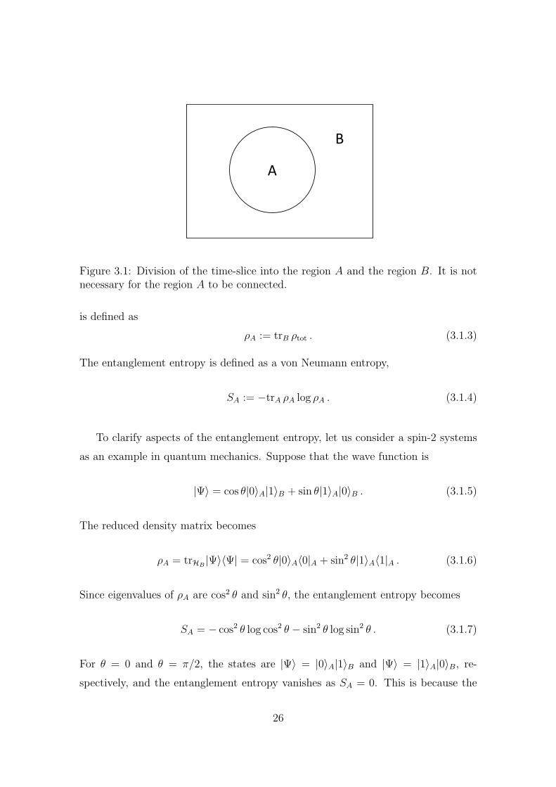
In quantum field theory, we take a time-slice of spacetime and define the Hilbert

space on it. The division of the total Hilbert space into two Hilbert space corresponds

to a division of the time-slice into a region A and a region B. See Fig. 3.1.

When the quantum system is described by a wave function |Ψ⟩, a total density

matrix is given by

ρtot = |Ψ⟩⟨Ψ| . (3.1.2)

By tracing out the degree of freedom of the region B, a reduced density matrix ρA

25

A

B

Figure 3.1: Division of the time-slice into the region A and the region B. It is notnecessary for the region A to be connected.

is defined as

ρA := trB ρtot . (3.1.3)

The entanglement entropy is defined as a von Neumann entropy,

SA := −trA ρA log ρA . (3.1.4)

To clarify aspects of the entanglement entropy, let us consider a spin-2 systems

as an example in quantum mechanics. Suppose that the wave function is

|Ψ⟩ = cos θ|0⟩A|1⟩B + sin θ|1⟩A|0⟩B . (3.1.5)

The reduced density matrix becomes

ρA = trHB|Ψ⟩⟨Ψ| = cos2 θ|0⟩A⟨0|A + sin2 θ|1⟩A⟨1|A . (3.1.6)

Since eigenvalues of ρA are cos2 θ and sin2 θ, the entanglement entropy becomes

SA = − cos2 θ log cos2 θ − sin2 θ log sin2 θ . (3.1.7)

For θ = 0 and θ = π/2, the states are |Ψ⟩ = |0⟩A|1⟩B and |Ψ⟩ = |1⟩A|0⟩B, re-spectively, and the entanglement entropy vanishes as SA = 0. This is because the

26

state is a pure state and the density matrix can be written by a direct product as

ρtot = ρA × ρB. For θ = ±π/4, the states are |Ψ⟩ = (|0⟩A|1⟩B ± |1⟩A|0⟩B)/√2, and

the entanglement entropy is SA = log 2. The 2 in the logarithm represents that

degree of freedom of the two-spin system is two. Entanglement entropies measures

the strength of the correlations between the subsystems A and B.

3.1.2 Replica method

Next, we would like to discuss the entanglement entropy in quantum field theory.

In quantum field theory it is difficult to calculate the von Neumann entropy (3.1.4)

directly because quantum field theory has infinite degrees of freedom defined on

each points of spacetime and the von Neumann entropy includes the logarithm of

the reduced density matrix. Then, we use analytical expressions of (3.1.4),

SA = − limn→1

∂

∂ntrAρ

nA = − lim

n→1

∂

∂nlog trAρ

nA , (3.1.8)

instead of calculating (3.1.4). We calculate trAρnA to evaluate the entanglement en-

tropy. We make a comment on the analytical continuation about n. n is assumed to

be integer and trAρnA is calculated for integer n. Nevertheless, when we calculate the

entanglement entropy, we assume that n is a real number. Although the analytical

continuation about n does not always give a correct result, counterexamples about

the entanglement entropy are not known yet. We don’t discuss the validity of the

analytical continuation about n anymore.

From now on, we explain a replica method [53]. Let us calculate the entanglement

entropy on the ground state |Ψ⟩1. For simplicity we consider Euclidean scalar field

theory. When the system is invariant under a time-translation, we can take x0 = 0

without loss of generality. The wave function for the ground state ⟨ϕ|Ψ⟩ is given by

Ψ[ϕ(x), x0 = 0] =1√Z

∫ ∏−∞<x0<0

∏x

Dϕ e−S[ϕ]δ[ϕ(0,x)− ϕ(x)] (3.1.9)

in path-integral representation. Here, S[ϕ] is an action, and Z is a partition function.

We insert 1/√Z as a normalisation of the wave function. A complex conjugate of

1We should write |0⟩ instead of |Ψ⟩ because we consider the vacuum state.

27

the wave function is defined as

Ψ∗[ϕ(x), x0 = 0] =1√Z

∫ ∏0<x0<∞

∏x

Dϕ e−S[ϕ]δ[ϕ(0,x)− ϕ(x)] . (3.1.10)

One can see that the wave function satisfies the normalisation condition∫DϕΨ∗[ϕ(x)]Ψ[ϕ(x)] = 1 . (3.1.11)

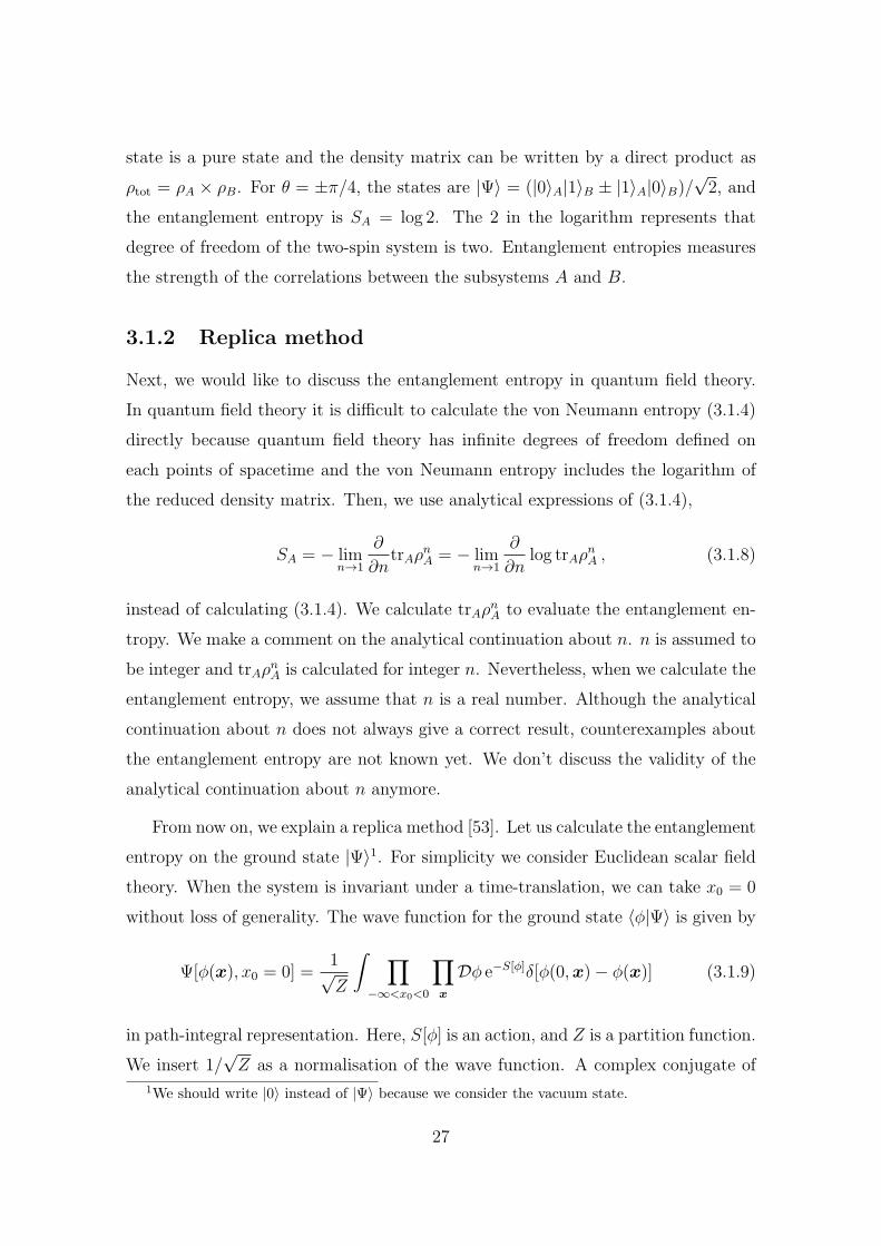
The reduced density matrix becomes

[ρA]ϕ−ϕ+ =1

Z

∫Dϕ e−S[ϕ]

∏x∈A

δ[ϕ(−0,x)− ϕ−(x)]δ[ϕ(+0,x)− ϕ+(x)] (3.1.12)

where ϕ+ and ϕ− are boundary conditions. The reduced density matrix [ρA]ϕ−ϕ+ is

represented pictorially in Fig. 3.2. By using this expression of the reduced density

Figure 3.2: Path-integral representation of the reduced density matrix. The otherdirections x2, · · · , xd−1 are omitted.

matrix, we obtain

trA ρnA =

1

Zn

∫ ∏x∈Σn

Dϕ e−S[ϕ] (3.1.13)

where Σn is an n-sheeted Riemann surface constructed as follows. Firstly, we prepare

n sheets of the original spacetime Σ. We number each spacetime Σ and each field

28

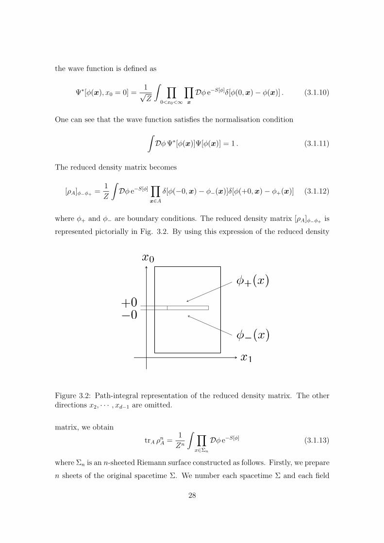
ϕ on each Σ, and refer to them as Σ(1), · · · ,Σ(n) and ϕ(1), · · · , ϕ(n), called replica

fields, respectively. Σn is the spacetime obtained by gluing each Σ with the boundary

condition2

ϕ(1)+ = ϕ

(2)− , ϕ

(2)+ = ϕ

(3)− , · · · , ϕ

(n)+ = ϕ

(1)− . (3.1.14)

See Fig. 3.3. From this expression, we notice that trA ρnA is the same as a partition

function on Σn (up to a normalisation).

Figure 3.3: n-sheeted Riemann surface Σn. For simplicity, the figure is n = 3 case.

Let us consider a free scalar field theory and calculate the entanglement entropy

for a half-plane for an example. We take the region A as x1 > 0. In this case, we take

n a fraction like 1/M whereM is integer, to make calculations very easy3. According

to the replica trick, we need to evaluate the partition function on R2/ZM × Rd−2.

In the following we show a detail calculation of the entanglement entropy.

An Euclidean Lagrangian is

L =1

2(∂µϕ(x))

2 +1

2m2ϕ(x)2 . (3.1.15)

2 For fermions, we need to take anti-periodic boundary condition instead of the periodic bound-ary condition.

3If we don’t take n a fraction, we need to diagonalize a set of replica fields (ϕ(1), · · · , ϕ(n)), andfind eigenvalues of a non-diagonal matrix. See [54], for detail.

29

By using a Fourier expansion of ϕ(x),

ϕ(x) =1

Vd

∑n

e−ikn·xϕ(kn) , (3.1.16)

the action can be written as

S =1

Vd

∑k0n>0

(k2n +m2)[(Reϕ(kn))2 + (Imϕ(kn))

2] . (3.1.17)

A measure of path integral is written as

Dϕ(x) =∏k0n>0

dReϕ(kn) d Imϕ(kn) (3.1.18)

in a Fourier space. In continuous limit of momentum, the summation of n is replaced

by an integral of momentum,

1

Vd

∑n

→∫

ddk

(2π)d. (3.1.19)

By using the above expressions, the partition function on Rd becomes

ZRd =

∫ ∏k0n>0

dReϕ(kn)d Imϕ(kn) exp (−S) = det

(πVd

k2n +m2

)1/2

. (3.1.20)

Then, the logarithm of the partition function can be calculated as

logZRd = log det

(πVd

k2n +m2

)1/2

= log∏kn

(πVd

k2n +m2

)1/2

= Tr log

(πVd

k2n +m2

)1/2

=∑kn

log

(πVd

k2n +m2

)1/2

= −1

2

∑kn

log(k2n +m2

)(ignore a factor coming fromπVd+1)

= −Vd2

∫ddk

(2π)dlog

(k2 +m2

)= Vd

∫ ∞

ε2

ds

2s

∫ddk

(2π)de−s(k2+m2)

30

= Vd

∫ ∞

ε2

ds

2s(4πs)−d/2e−sm2

(3.1.21)

where we use the Schwinger’s parametrization,

logα = −∫ ∞

0

dt

te−αt . (3.1.22)

Identified

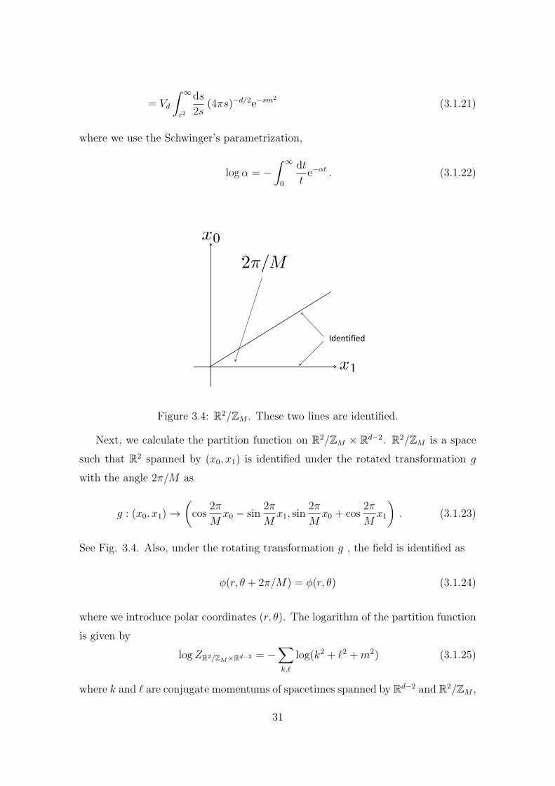
Figure 3.4: R2/ZM . These two lines are identified.

Next, we calculate the partition function on R2/ZM × Rd−2. R2/ZM is a space

such that R2 spanned by (x0, x1) is identified under the rotated transformation g

with the angle 2π/M as

g : (x0, x1)→(cos

2π

Mx0 − sin

2π

Mx1, sin

2π

Mx0 + cos

2π

Mx1

). (3.1.23)

See Fig. 3.4. Also, under the rotating transformation g , the field is identified as

ϕ(r, θ + 2π/M) = ϕ(r, θ) (3.1.24)

where we introduce polar coordinates (r, θ). The logarithm of the partition function

is given by

logZR2/ZM×Rd−2 = −∑k,ℓ

log(k2 + ℓ2 +m2) (3.1.25)

where k and ℓ are conjugate momentums of spacetimes spanned by Rd−2 and R2/ZM ,

31

respectively. The continuous limit of the summation of k gives

∑k

→ Vd−2

∫dd−2k

(2π)d−2(3.1.26)

as before. In order to perform the summation of ℓ, we insert a projection operator∑M−1j=0 gj/M into the summation of ℓ. That is, the summation is written as

∑ℓ

log(k2 + ℓ2 +m2) =

∫d2ℓ

(2π)2⟨ℓ| log(k2 + ℓ2 +m2)

M−1∑j=0

gj

M|ℓ⟩ . (3.1.27)

g operates on the ket vector |ℓ⟩ = |ℓ0, ℓ1⟩, which is normalised as ⟨ℓ|ℓ′⟩ = (2π)2δ2(ℓ−ℓ′)/V2 and ⟨ℓ|ℓ⟩ = 1, as

g|ℓ0, ℓ1⟩ =∣∣∣∣cos 2πM ℓ0 − sin

2π

Mℓ1, sin

2π

Mℓ0 + cos

2π

Mℓ1

⟩. (3.1.28)

By introducing the Schwinger’s parametrization, the partition function becomes

logZR2/ZM×Rd−2 = Vd−2V2

∫ ∞

ε2

ds

2s

∫dd−2k

(2π)d−2e−sk2−sm2

∫d2ℓ

(2π)2

M−1∑j=0

⟨ℓ|e−sℓ2 gj

M|ℓ⟩

(3.1.29)

For j = 0, it is just the partition function on Rd divided byM . For j = 0, we obtain

V2

∫d2ℓ

(2π)2⟨ℓ|e−sℓ2 g

j

M|ℓ⟩ = 1

M

∫d2ℓ e−sℓ2δ2(ℓ− gj · ℓ) = 1

4M sin2 πjM

. (3.1.30)

By using the identity,M−1∑j=1

1

sin2 πjM

=M2 − 1

3, (3.1.31)

we obtain the partition function,

logZR2/ZM×Rd−2 = Vd−2M2 − 1

12M

∫ ∞

ε2

ds

2s

∫dd−2k

(2π)d−2e−sk2−sm2

+1

MlogZRd

= Vd−2M2 − 1

12M

∫ ∞

ε2

ds

2s

e−sm2

(4πs)d−22

+1

MlogZRd . (3.1.32)

32

The entanglement entropy becomes

SA = − limM→1

∂

∂(1/M)

(logZR2/ZM×Rd−2 − 1

MlogZRd

)=

Vd−2

6(d− 2)(4π)d−22

· 1

εd−2+O(ε−(d−4)) . (3.1.33)

This result shows that the entanglement entropy satisfies the area law,

SA = γArea of ∂A

εd−2+O(ε−(d−4)) , (3.1.34)

where γ is a numerical constant which depends on the detail of the theory and ∂A a

circumference of A. Finally we comment on physical quantity in the entanglement

entropy. It is known that the entanglement entropy behaves as

SA = p1ℓd−2

εd−2+ p3

ℓd−4

εd−4+ · · ·+

pd−2ℓε+ pd d : odd

pd−3ℓ2

ε2+ q log

(ℓε

)d : even

(3.1.35)

where p and q are constants and depend on the shape of the entanglement surface.

ℓ is a typical size of the region A. The most divergent term which shows the area

law of the entanglement entropy is not a physical quantity because it depends on

the cut-off parameter ε. That is, if we change the cut-off parameter, the coefficient

is changed. For the same reason, other divergent terms are not physical quantities,

also. On the other hand, the constant term and the logarithm term are physical. In

two dimensional case, the coefficient of the logarithm term is a central charge which

represents degree of freedom.

3.2 Holographic entanglement entropy

We discuss the entanglement entropy in the context of the holography. A holographic

dual of the entanglement entropy is given by the Ryu-Takayanagi formula [17, 18].

The Ryu-Takayanagi formula states that the entanglement entropy for the region A

is given by

SA =Area of γA

4GN

, (3.2.1)

33

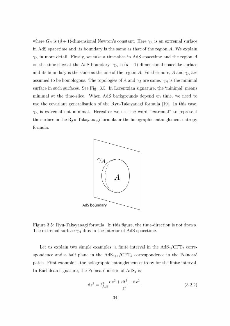
where GN is (d+1)-dimensional Newton’s constant. Here γA is an extremal surface

in AdS spacetime and its boundary is the same as that of the region A. We explain

γA in more detail. Firstly, we take a time-slice in AdS spacetime and the region A

on the time-slice at the AdS boundary. γA is (d − 1)-dimensional spacelike surface

and its boundary is the same as the one of the region A. Furthermore, A and γA are

assumed to be homologous. The topologies of A and γA are same. γA is the minimal

surface in such surfaces. See Fig. 3.5. In Lorentzian signature, the ‘minimal’ means

minimal at the time-slice. When AdS backgrounds depend on time, we need to

use the covariant generalisation of the Ryu-Takayanagi formula [19]. In this case,

γA is extremal not minimal. Hereafter we use the word “extremal” to represent

the surface in the Ryu-Takayanagi formula or the holographic entanglement entropy

formula.

AdS boundary

Figure 3.5: Ryu-Takayanagi formula. In this figure, the time-direction is not drawn.The extremal surface γA dips in the interior of AdS spacetime.

Let us explain two simple examples; a finite interval in the AdS3/CFT2 corre-

spondence and a half plane in the AdSd+1/CFTd correspondence in the Poincare

patch. First example is the holographic entanglement entropy for the finite interval.

In Euclidean signature, the Poincare metric of AdS3 is

ds2 = ℓ2AdS

dz2 + dt2 + dx2

z2. (3.2.2)

34

The boundary of the region A is given by (t, x) = (0,−R) and (t, x) = (0, R). The

extremal surface is given by

z =√R2 − x2 . (3.2.3)

See Fig. 3.6. The induced metric on the extremal surface is

ds2 =ℓ2AdSR

2dz2

4z2(R2 − z2). (3.2.4)

Then, by using the Ryu-Takayanagi formula the entanglement entropy becomes

SA =1

4GN

∫ds =

ℓAdSR

4GN

∫ R

ε

dz

z√R2 − z2

=ℓAdS

2GN

log

(R

ε

). (3.2.5)

Here ε is a cut-off parameter and corresponds to a UV cut-off in the dual CFT. By

using the well-known result about the central charge in the AdS3/CFT2 correspon-

dence,

c =3ℓAdS

2GN

, (3.2.6)

we obtain the logarithm behaviour of the entanglement entropy

SA =c

6log

(R

ε

). (3.2.7)

We skip the discussion about the entanglement entropy in two dimensional CFTs.

We can derive (3.2.7) by using the replica trick.

Next example is the holographic entanglement entropy of the half plane. See

Fig. 3.7. From the symmetry, the extremal surface is given by

0 ≤ z <∞ . (3.2.8)

According to the Ryu-Takayanagi formula, the holographic entanglement entropy of

the half plane is given by

SA =Vd−2

4GN

∫ ∞

ε

dz

(ℓAdS

z

)d−1

=Vd−2ℓ

d−1AdS

4GN(d− 2)· 1

εd−2(3.2.9)

35

A

Extremal surface

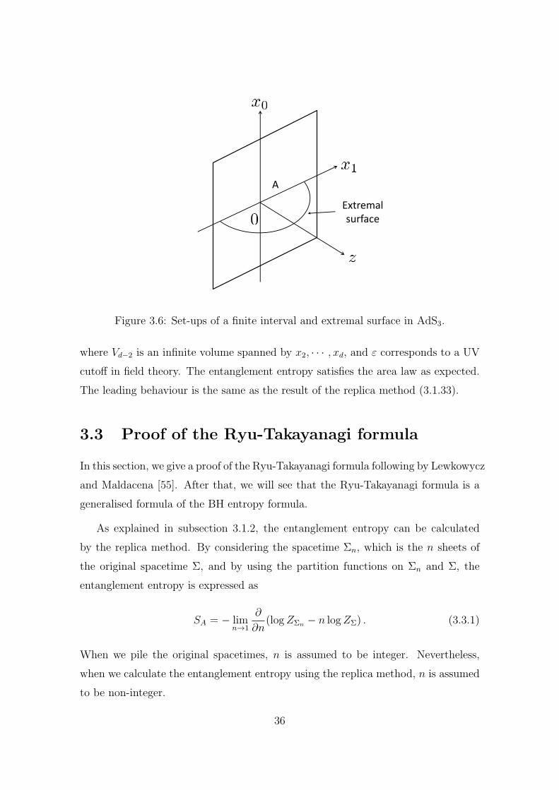
Figure 3.6: Set-ups of a finite interval and extremal surface in AdS3.

where Vd−2 is an infinite volume spanned by x2, · · · , xd, and ε corresponds to a UV

cutoff in field theory. The entanglement entropy satisfies the area law as expected.

The leading behaviour is the same as the result of the replica method (3.1.33).

3.3 Proof of the Ryu-Takayanagi formula

In this section, we give a proof of the Ryu-Takayanagi formula following by Lewkowycz

and Maldacena [55]. After that, we will see that the Ryu-Takayanagi formula is a

generalised formula of the BH entropy formula.

As explained in subsection 3.1.2, the entanglement entropy can be calculated

by the replica method. By considering the spacetime Σn, which is the n sheets of

the original spacetime Σ, and by using the partition functions on Σn and Σ, the

entanglement entropy is expressed as

SA = − limn→1

∂

∂n(logZΣn − n logZΣ) . (3.3.1)

When we pile the original spacetimes, n is assumed to be integer. Nevertheless,

when we calculate the entanglement entropy using the replica method, n is assumed

to be non-integer.

36

A

B

Extremal surface

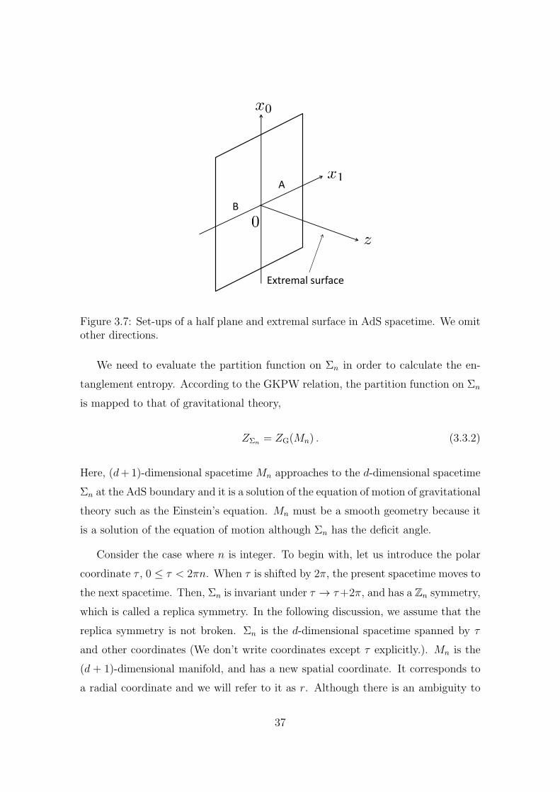
Figure 3.7: Set-ups of a half plane and extremal surface in AdS spacetime. We omitother directions.

We need to evaluate the partition function on Σn in order to calculate the en-

tanglement entropy. According to the GKPW relation, the partition function on Σn

is mapped to that of gravitational theory,

ZΣn = ZG(Mn) . (3.3.2)

Here, (d+1)-dimensional spacetime Mn approaches to the d-dimensional spacetime

Σn at the AdS boundary and it is a solution of the equation of motion of gravitational

theory such as the Einstein’s equation. Mn must be a smooth geometry because it

is a solution of the equation of motion although Σn has the deficit angle.

Consider the case where n is integer. To begin with, let us introduce the polar

coordinate τ , 0 ≤ τ < 2πn. When τ is shifted by 2π, the present spacetime moves to

the next spacetime. Then, Σn is invariant under τ → τ+2π, and has a Zn symmetry,

which is called a replica symmetry. In the following discussion, we assume that the

replica symmetry is not broken. Σn is the d-dimensional spacetime spanned by τ

and other coordinates (We don’t write coordinates except τ explicitly.). Mn is the

(d + 1)-dimensional manifold, and has a new spatial coordinate. It corresponds to

a radial coordinate and we will refer to it as r. Although there is an ambiguity to

37

choose r, we select r such that τ direction shrinks smoothly at r = 0. In this case,

the metric behaves

ds2 ≃ dr2 +r2

n2dτ 2 + · · · (3.3.3)

near r = 0. · · · represents other directions. Since the period of τ is 2πn, there is no

conical singularity at r = 0. Also, we impose the replica symmetry on fields as

ϕ(τ + 2π) = ϕ(τ) , (3.3.4)

where ϕ represents all fields included in gravity such as metric or scalar fields.

Note that the logarithm of ZG(Mn) can be written as

logZG(Mn) = n logZG(Mn) (3.3.5)

where Mn is division into n parts of the spacetime Mn. Since Mn has the period

2π, a conical singularity exists at r = 0. Nevertheless, we ignore a contribution

coming from the conical singularity when we calculate the partition function on Mn.

When we calculate the entanglement entropy, we need to perform the analytical

continuation about n. In that case, we define ZG(Mn) for general n by using the

relation (3.3.5).

We introduce a (d+1)-dimensional manifold Nn, and decompose the calculation

of the entanglement entropy as follows;

logZΣn − n logZΣ = n logZG(Mn)− n logZG(M)

= −n(SG(Mn)− SG(Nn)

)− n

(SG(Nn)− SG(M)

). (3.3.6)

Here Nn is a smooth spacetime corresponding to M except a vicinity of r = 0 and

Mn at r < ε for an arbitrary small quantity ε. Nn does not satisfy the equation of

motion, and there are many candidates such a spacetime. We choose one of them.

To calculate the entanglement entropy, we need to find O(n − 1) contributions

in (3.3.6) in the n → 1 limit. The first parentheses in (3.3.6) gives no contribution

to the entanglement entropy because Mn is the solution of the equation of motion

38

and a deviation O(n− 1) of the action does not appear,

limn→1

(SG(Mn)− SG(Nn)

)= 0 . (3.3.7)

In the second parentheses in (3.3.6), the O(n− 1) contribution is coming from the

region r < ϵ. nNn has no conical singularity but nM has a conical singularity with

a deficit angle 2π(1− n). Then, a difference between Ricci scalars becomes

RnN −RnM = 4π(1− n) · δ2(r) . (3.3.8)

The proof is given in Appendix B.

Summarizing the above discussion, we obtain

logZΣn − n logZΣ = −n(SG(Nn)− SG(M)

)=

1− n4GN

∫γA

√g . (3.3.9)

where γA is (d− 1)-dimensional spacelike surface at r = 0 and g the determinant of

the induced metric on r = 0. According to the replica trick, we finally obtain the

entanglement entropy

SA =1

4GN

∫γA

√g (3.3.10)

Furthermore, it is shown that γA is an extremal surface from the equation of motion.

This is a proof of the Ryu-Takayanagi formula.

Finally, we comment on the relation between the BH entropy and the holographic

entanglement entropy. Consider a Euclidean gravity and its black hole solution. In

this case, the boundary condition for the metric or other fields, is invariant a U(1)

symmetry along the τ direction. It is known that the BH entropy,

SBH = − limn→1

∂

∂n(logZG(Mn)− n logZG(M1)) , (3.3.11)

is equal to the area of the co-dimension two surface which is invariant the U(1)

symmetry. This co-dimension two surface is a horizon of the black hole.

In the holographic entanglement entropy formula, the U(1) symmetry is replaced

by the replica symmetry Zn, and the boundary is changed from the horizon to the

39

asymptotically AdS boundary. In this sense, the Ryu-Takayanagi formula can be

regarded as a generalised quantity of the BH entropy.

40

Chapter 4

Holographic Entanglement

Entropy in Einstein Gravity on dS

4.1 Proposal

As noted in the Introduction, it is known that the BH entropy is given by an event

horizon area divided by four times Newton’s constant,

SBH =Horizon Area

4GN

. (4.1.1)

The BH entropy formula holds not only in asymptotically flat spacetime or AdS

spacetime but also in asymptotically dS spacetime. As reviewed in the previous

chapter, the holographic entanglement entropy can be regarded as a generalised

quantity of the BH entropy [55], and it is given by an area of an extremal surface

divided by four times Newton’s constant,

SHEE =Extremal Surface Area

4GN

. (4.1.2)

Then it is natural to expect that a formula similar to the Ryu-Takayanagi formula

holds even in dS spacetime as the BH entropy formula.

Thus we need to find “extremal surfaces” which extend to the future infinity I+

, where the dual CFTs are assumed to live, in Einstein gravity on dS spacetime in

41

order to construct the holographic entanglement entropy formula in the dS/CFT

correspondence. The notion of the extremal surface is however obscure. If the

surfaces were space-like, their area would be smaller and smaller as the surfaces

approached null. If the surfaces were time-like, their area would be imaginary, and

the surfaces would not be closed in general. We discuss this issue based on analytic

continuation because the analytic continuation enables us to obtain surfaces in dS

spacetime, which satisfy the equation of motion obtained from the variation of the

area functional. Our proposal is that the extremal surfaces in dS spacetime are given

by the analytic continuation of extremal surfaces in EAdS spacetime. This proposal

allows for extremal surfaces which extend in complex-valued coordinate spacetime,

and lets us find complex surfaces as extremal surfaces. In the next chapter, we will

check the consistency of our proposal using a toy model.

Extremal surface

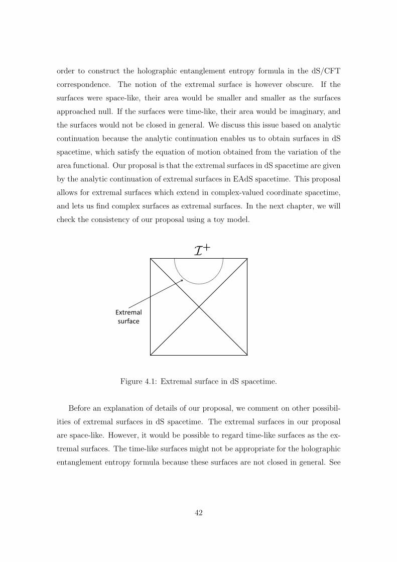
Figure 4.1: Extremal surface in dS spacetime.

Before an explanation of details of our proposal, we comment on other possibil-

ities of extremal surfaces in dS spacetime. The extremal surfaces in our proposal

are space-like. However, it would be possible to regard time-like surfaces as the ex-

tremal surfaces. The time-like surfaces might not be appropriate for the holographic

entanglement entropy formula because these surfaces are not closed in general. See

42

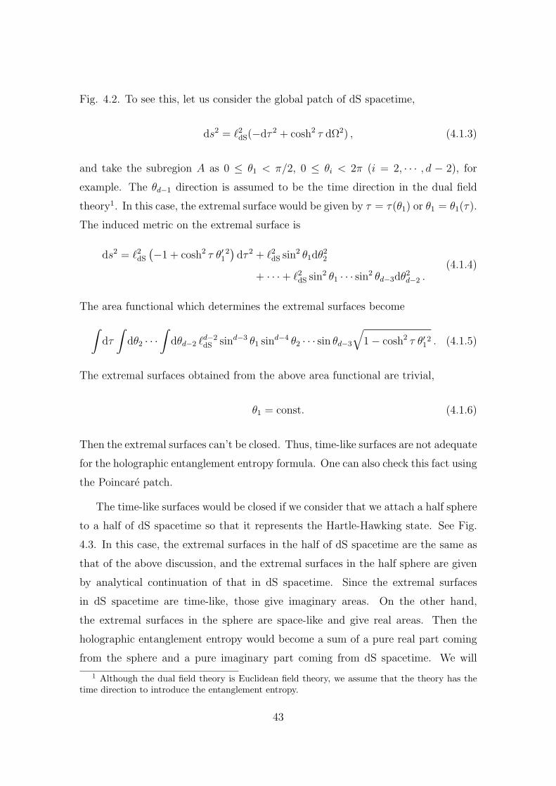
Fig. 4.2. To see this, let us consider the global patch of dS spacetime,

ds2 = ℓ2dS(−dτ 2 + cosh2 τ dΩ2) , (4.1.3)

and take the subregion A as 0 ≤ θ1 < π/2, 0 ≤ θi < 2π (i = 2, · · · , d − 2), for

example. The θd−1 direction is assumed to be the time direction in the dual field

theory1. In this case, the extremal surface would be given by τ = τ(θ1) or θ1 = θ1(τ).

The induced metric on the extremal surface is

ds2 = ℓ2dS(−1 + cosh2 τ θ′1

2)dτ 2 + ℓ2dS sin

2 θ1dθ22

+ · · ·+ ℓ2dS sin2 θ1 · · · sin2 θd−3dθ

2d−2 .

(4.1.4)

The area functional which determines the extremal surfaces become∫dτ

∫dθ2 · · ·

∫dθd−2 ℓ

d−2dS sind−3 θ1 sin

d−4 θ2 · · · sin θd−3

√1− cosh2 τ θ′1

2 . (4.1.5)

The extremal surfaces obtained from the above area functional are trivial,

θ1 = const. (4.1.6)

Then the extremal surfaces can’t be closed. Thus, time-like surfaces are not adequate

for the holographic entanglement entropy formula. One can also check this fact using

the Poincare patch.

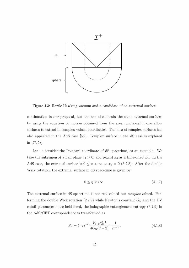
The time-like surfaces would be closed if we consider that we attach a half sphere

to a half of dS spacetime so that it represents the Hartle-Hawking state. See Fig.

4.3. In this case, the extremal surfaces in the half of dS spacetime are the same as

that of the above discussion, and the extremal surfaces in the half sphere are given

by analytical continuation of that in dS spacetime. Since the extremal surfaces

in dS spacetime are time-like, those give imaginary areas. On the other hand,

the extremal surfaces in the sphere are space-like and give real areas. Then the

holographic entanglement entropy would become a sum of a pure real part coming

from the sphere and a pure imaginary part coming from dS spacetime. We will

1 Although the dual field theory is Euclidean field theory, we assume that the theory has thetime direction to introduce the entanglement entropy.

43

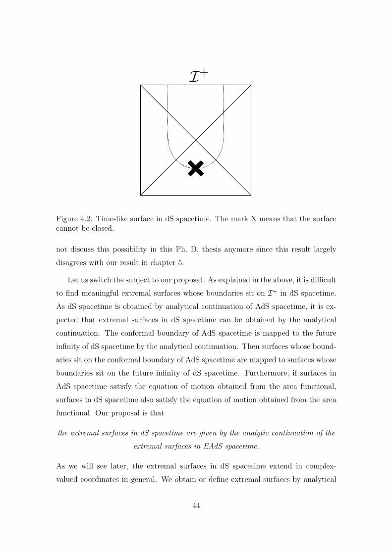
Figure 4.2: Time-like surface in dS spacetime. The mark X means that the surfacecannot be closed.

not discuss this possibility in this Ph. D. thesis anymore since this result largely

disagrees with our result in chapter 5.

Let us switch the subject to our proposal. As explained in the above, it is difficult

to find meaningful extremal surfaces whose boundaries sit on I+ in dS spacetime.

As dS spacetime is obtained by analytical continuation of AdS spacetime, it is ex-

pected that extremal surfaces in dS spacetime can be obtained by the analytical

continuation. The conformal boundary of AdS spacetime is mapped to the future

infinity of dS spacetime by the analytical continuation. Then surfaces whose bound-

aries sit on the conformal boundary of AdS spacetime are mapped to surfaces whose

boundaries sit on the future infinity of dS spacetime. Furthermore, if surfaces in

AdS spacetime satisfy the equation of motion obtained from the area functional,

surfaces in dS spacetime also satisfy the equation of motion obtained from the area

functional. Our proposal is that

the extremal surfaces in dS spacetime are given by the analytic continuation of the

extremal surfaces in EAdS spacetime.

As we will see later, the extremal surfaces in dS spacetime extend in complex-

valued coordinates in general. We obtain or define extremal surfaces by analytical

44

dS

Sphere

Figure 4.3: Hartle-Hawking vacuum and a candidate of an extremal surface.

continuation in our proposal, but one can also obtain the same extremal surfaces

by using the equation of motion obtained from the area functional if one allow

surfaces to extend in complex-valued coordinates. The idea of complex surfaces has

also appeared in the AdS case [56]. Complex surface in the dS case is explored

in [57,58].

Let us consider the Poincare coordinate of dS spacetime, as an example. We

take the subregion A a half plane x1 > 0, and regard xd as a time-direction. In the

AdS case, the extremal surface is 0 ≤ z < ∞ at x1 = 0 (3.2.8). After the double

Wick rotation, the extremal surface in dS spacetime is given by

0 ≤ η < i∞ . (4.1.7)

The extremal surface in dS spacetime is not real-valued but complex-valued. Per-

forming the double Wick rotation (2.2.9) while Newton’s constant GN and the UV

cutoff parameter ε are held fixed, the holographic entanglement entropy (3.2.9) in

the AdS/CFT correspondence is transformed as

SA = (−i)d−1 Vd−2ℓd−1dS

4GN(d− 2)· 1

εd−2. (4.1.8)

45

In conclusion, the holographic entanglement entropy in the dS/CFT correspondence

is given by that of the AdS/CFT correspondence, where ℓAdS is replaced by ℓdS, times

(−i)d−1. It can become positive, negative, or imaginary for the dimension.

4.2 Extremal surfaces in asymptotically dS space-

time

In the previous section, we proposed the holographic entanglement entropy formula

in the dS/CFT correspondence via the double Wick rotation. And we found the

extremal surfaces in Poincare dS spacetime and obtained the holographic entangle-

ment entropy, as an example. In this section, we comment on extremal surfaces in

a more general set of asymptotically dS spacetime.

To define extremal surfaces in asymptotically dS spacetime, we need to find a

double Wick rotation between the asymptotically dS spacetime and the correspond-

ing asymptotically EAdS spacetime. One Wick rotation is

ℓdS → iℓAdS (4.2.1)

to make the cosmological constant positive. A second analytic continuation is con-

cerned with the time coordinate in asymptotically dS spacetime and the radial direc-

tion in corresponding asymptotically EAdS spacetime. Since the second analytical

continuation depends on coordinate systems, we cannot typically say the second

analytical continuation concretely like (4.2.1).

Our proposal is that the holographic entanglement entropy in the dS/CFT cor-

respondence is defined as

SHEE :=AreadS4GN

. (4.2.2)

Here AreadS is the area of the “extremal surfaces” in asymptotically dS spacetime

defined as follows. Firstly, we find extremal surfaces in the corresponding asymptot-

ically EAdS spacetime. Next, performing the double Wick rotation of the extremal

surfaces in asymptotically EAdS spacetime, we define “extremal surfaces” in asymp-

totically dS spacetime. As in the previous section, the extremal surfaces in asymp-

46

totically dS spacetime are complex-valued in general although the extremal surfaces

in asymptotically EAdS spacetime are real-valued. Then, AreadS is the area of the

extremal surfaces in asymptotically dS spacetime. The holographic entanglement

entropy (4.2.2) is uniquely defined by using the extremal surfaces in asymptotically

EAdS spacetime.

It is intriguing to apply our proposal for the asymptotically dS spacetime case to

a Schwarzschild dS black hole. By analogy from the AdS/CFT correspondence case,

it is expected that the holographic entanglement entropy includes the contribution

of the black hole. We could obtain an interpretation of the black hole entropy in dS

spacetime.

47

Chapter 5

Entanglement Entropy in the

Sp(N) Model

Since the CFT dual to Einstein gravity on dS spacetime is not known yet, we

analyze the Sp(N) model as a toy model. Since the Sp(N) model is the holographic

dual of Vasiliev’s higher-spin gauge theory on dS spacetime, we can quantitatively

compare such results only with Vasiliev’s higher-spin gauge theory, not with Einstein

gravity. However, it is natural to expect that their basic qualitative behaviours do

not change between these two theories. Then, we explore the Sp(N) model [46, 47]

in this chapter.

5.1 Sp(N) model

The interacting Sp(N) model on a Lorentzian spacetime with the metric gµν is

defined by the action

S = −1

2

∫ddx√−g

(Ωabg

µν∂µχa∂νχ

b +m2Ωabχaχb + λ(Ωabχ

aχb)2), (5.1.1)

where χa (a = 1, · · · , N) are anticommuting scalars, N an even integer, m mass, λ

coupling constant and

Ωab =

0 1N/2×N/2

−1N/2×N/2 0

, (5.1.2)

48

the anti-symmetric matrix [46]. The metric sign is mostly plus. Here we ignore

whether the theory can be renormalised or not. When d = 4, the theory is renor-

malisable and violates spin-static theorem.

By introducing

ηa = χa + iχa+N2 , ηa = −iχa − χa+N

2

(a = 1, · · · , N

2

), (5.1.3)

the action is rewritten as

S = −∫ddx√−g

(gµν∂µη ∂νη +m2ηη + λ(ηη)2

). (5.1.4)

When we write the action in terms of η and η, the action seems to be that of complex

scalars. We will use both actions.

Let us quantize the Sp(N) model on flat spacetime. Conjugate momentum fields

are introduced as

πη :=∂L

∂(∂0η)= −∂0η , πη :=

∂L∂(∂0η)

= ∂0η , (5.1.5)

respectively. Here L is a Lagrangian, and derivatives in terms of η and η mean

left-derivatives. For simplicity, we use π and π instead of πη and πη, respectively.

Then, a Hamiltonian is given by

H : = ∂0η · π + ∂0η · π − L

= ππ + ∂iη∂iη +m2ηη + λ(ηη)2 . (5.1.6)

Anti-commutation relations at the same time are given by

ηa(t,x), πb(t,x′) = ηa(t,x), πb(t,x′) = iδabδd−1(x− x′) . (5.1.7)

From now on, we focus on the free Sp(N) model, for simplicity. Fourier trans-

formations of the fields are

η(x) =

∫dd−1k

(2π)d−1√2ωk

(b†k,−eik·x + bk,+e

−ik·x) , (5.1.8)

49

η(x) =

∫dd−1k

(2π)d−1√2ωk

(−bk,−eik·x + b†k,+e−ik·x) , (5.1.9)

where k · x = −ωkt+ k ·x. By inserting Fourier transformations (5.1.8) and (5.1.9)

to the anti-commutation relations (5.1.7), the anti-commutation relations in terms

of bk,± become

bk,+, b†k′,+ = bk,−, b†k′,− = δd−1(k − k′) . (5.1.10)

Other anti-commutation relations vanish. The Hamiltonian becomes

H =

∫dd−1k ωk(b

†k,+bk,+ − bk,−b

†k,−)

=

∫dd−1k ωk(b

†k,+bk,+ + b†k,−bk,−) + const. (5.1.11)

in terms of the creation and annihilation operators bk,± and b†k,±. The vacuum state

|0⟩ is defined such that it is annihilated by the operators bk,±,

bk,±|0⟩ = 0 . (5.1.12)

Let’s discuss a pseudo-unitarity of the Sp(N) model. The Sp(N) model is not

unitary in the sense that the inner product ⟨ψ|ϕ⟩ is not preserved under time evo-

lution because the Hamiltonian is not Hermite,

H† = H . (5.1.13)

Nevertheless, Sp(N) model has a special property and we can define a new inner

product preserved under time evolution. Firstly, we introduce a unitary operator C

which satisfies

C†C = 1 , C† = C . (5.1.14)

The vacuum |0⟩ is assumed to be invariant, C|0⟩ = |0⟩. We define that the unitary

50

operator C operates on the fields as1

CηC = −η . (5.1.15)

In terms real fields χa and χa+N/2, they transforms as

CχaC = χa+N/2 , Cχa+N/2C = χa . (5.1.16)

The unitary operator C operates on the creation and annihilation operators as

Cb±C = ∓b†± . (5.1.17)

Although the Hamiltonian is not Hermite, the Hamiltonian satisfies the relation,

H† = CHC . (5.1.18)

We refer to it as pseudo unitarity. We introduce a new inner product ⟨ψ|ϕ⟩C as

⟨ψ|ϕ⟩C := ⟨ψ|C|ϕ⟩ . (5.1.19)

We refer to the new norm as C-norm. This inner product is preserved under time

evolution,

⟨ψ(t)|ϕ(t)⟩C := ⟨ψ|eiH†tCe−iHt|ϕ⟩ = ⟨ψ|ϕ⟩C , (5.1.20)

as opposed to the usual inner product ⟨ψ|ϕ⟩.

5.2 Entanglement entropy

In this section, we introduce the entanglement entropy in the Sp(N) model [1, 2].

Naively, the density matrix is given by ρtot = |Ψ⟩⟨Ψ| and the entanglement entropy

is defined as a von-Neumann entropy SA = −trA ρA log ρA with a reduced density

1In [46], the unitary operator is defined to operate on η and η as CηC = η†. But, if we defineso, we would obtain CχaC = (χa+N/2)† and Cχa+N/2C = −(χa)†. This is a contradiction. Weshould define operations by C as CηC = ±η. There is an ambiguity to choose a sign and we adoptCηC = −η in this Ph. D. thesis not to include negative signs in (5.1.16).

51

matrix ρA = trAρtot. However, it seems that this definition is inadequate because of

H† = H as we will see below. To compute [ρtot]χ−χ+ , we write ⟨χ−|Ψ⟩ and ⟨Ψ|χ+⟩ inpath-integral. Doing the same calculation, we obtain the wave function at x0 = 0,

⟨χ−|Ψ⟩ =∫ ∏

−∞<x0<0

Dχ e−S[χ]δ(χ(0,x)− χ−(x)) , (5.2.1)

in Euclidean signature. Unlike ⟨χ−|Ψ⟩, ⟨Ψ|χ+⟩ is different from that of standard

scalar field theory. A complex conjugate of the wave function at t becomes

⟨Ψ(t)| = ⟨Ψ(t0)|eiH†(t−t0) , (5.2.2)

in Lorentzian signature. Since the Hamiltonian is not Hermite, we cannot express the

vacuum state using the path integral. The complex conjugate of the wave function

can not be expressed in path-integral representation.

Instead of ρtot = |Ψ⟩⟨Ψ|, we use a new density matrix,

ρCtot := |Ψ⟩⟨Ψ|C . (5.2.3)

As long as there is no confusion, we use ρtot instead of ρCtot. Next task is to evaluate

⟨Ψ|C|χ+⟩ to calculate a reduced density matrix. It is evaluated as

⟨Ψ(t0)|C|χ+⟩ ∼∫ ∏

t0<x0<∞

Dχ eiS[χ]δ(χ(0,x)− χ+(x)) (5.2.4)

in Lorentzian signature. Here, we assume that the state is a vacuum state. When the

state is an exciting state, we need to some operators in path integral. In Euclidean

signature, the wave function and its complex conjugate with the pseudo unitary

operator C are

⟨χ−|Ψ⟩ =1√Z ′

∫ ∏−∞<x0<0

Dχ e−S[χ]δ(χ(0,x)− χ−(x)) , (5.2.5)

⟨Ψ|C|χ+⟩ =1√Z ′

∫ ∏0<x0<∞

Dχ e−S[χ]δ(χ(0,x)− χ+(x)) , (5.2.6)

where Z ′ is a normalisation factor such that trAρA = 1. As we will see later, Z ′ is

52

just a partition function Z when we impose the periodic boundary condition on χ.

On the other hand, Z ′ is different from the partition function when we impose the

anti-periodic boundary condition on χ like fermion. By using (5.2.5) and (5.2.6),

the path-integral representation of the reduced density matrix is given by,

[ρA]χ−χ+ =1

Z ′

∫Dχ e−S[χ]

∏x∈A

δ(χ(−0,x)− χ−(x))δ(χ(+0,x)− χ+(x)) . (5.2.7)

Then, the entanglement entropy can be defined as

SA = −trA ρA log ρA . (5.2.8)

In the following, we calculate the entanglement entropy for a half plane.

Let us consider the periodic boundary condition case, firstly. The entanglement

entropy for the half plane on Rd can be calculated from partition functions on

R2/ZM × Rd−2 and Rd as explained in section 3.1.2,

SPA = − lim

M→1

∂

∂(1/M)

(logZR2/ZM×Rd−2 − 1

MlogZRd

), (5.2.9)

where the index P means periodic. The logarithm of the partition function is eval-

uated as

logZRd = log

∫Dχ e−S = NVd log

∫ddk

(2π)dlog k2 , (5.2.10)

where Vd is the volume of Rd. This result is minus that of standard scalar field

theories. It comes from the statics of the fields. Since logZR2/ZM×Rd−2 is also minus

that of the standard scalar field theories, the entanglement entropy is given by

SPA = − NVd−2

6(d− 2)(4π)d−22

· 1

εd−2, (5.2.11)

where Vd−2 is a (d− 2)-dimensional infinite volume and ε a UV cutoff. The entan-

glement entropy (5.2.11) is minus that of standard scalar field theories. We can also

obtain similar results for arbitrary subsystems on Rd or other curved spacetimes.

53

Next, we consider the anti-periodic case. In this case, the fields χa transforms as

χa(r, θ + 2π) = −χa(r, θ) . (5.2.12)

The logarithm of the partition function on Rd is evaluated as

logZRd = log

∫Dχ e−S = −NVd log

∫ddk

(2π)dlog k2 . (5.2.13)

Since we impose the anti-periodic boundary condition (5.2.12) instead of the periodic

boundary condition, the negative sign appears in (5.2.13). We also obtain a similar

behaviour of the partition function on R2/ZM × Rd−2. Then, the entanglement

entropy becomes

SAPA =

NVd−2

6(d− 2)(4π)d−22

· 1

εd−2, (5.2.14)

where the index AP means anti-periodic. We can also generalize it to arbitrary

entanglement surfaces on arbitrary curved spacetimes.

5.3 Comparison with A Toy CFT Model

Let us compare the result in the previous section with our proposal discussed in

chapter 4. According to our proposal, we obtain the holographic entanglement

entropy (4.1.8),

SA = (−i)d−1 Vd−2ℓd−1dS

4GN(d− 2)· 1

εd−2. (5.3.1)

Note that the holographic entanglement entropy has a coefficient (−i)d−1 in general.

In [1], we adopt the entanglement entropy with the periodic boundary condition on

the grounds that the fundamental fields of the Sp(N) model are scalar. We have

obtained the entanglement entropy,

SPA = − NVd−2

6(d− 2)(4π)d−22

· 1

εd−2. (5.3.2)

Note that SPA is minus that of standard scalar field theories. The result (5.2.11)

holds for any dimensions. Note however that it is known that the duality between

54

Vasiliev’s higher-spin gauge theory and the Sp(N) model holds only when d = 3.

Summarizing the above, the holographic entanglement entropy behaves as SA ∝(−i)d−1 in dSd+1 (4.1.8), and the entanglement entropy is given by minus that of

standard field theories (5.2.11). This result may suggest that the dSd+1/CFTd corre-

spondence makes senses only when d ∈ 4Z− 1. Note that the most interesting case,

the dS4/CFT3 correspondence, is included, while the simplest case, the dS3/CFT2

correspondence, is excluded. This is consistent with results in subsection 5.2 in [27],

which we reviewed in “surface/state operator” in subsection 2.2.2.

Our proposal has been checked only in the simple case, where the subsystem is the

half plane. We need to check our proposal in more nontrivial setups with circular or

some other shaped entanglement surfaces for example. However, it is expected that

our proposal holds in any entanglement surfaces because the factor (−i)d−1 appears

in Einstein gravity via the double Wick rotation (4.1.8), and the minus sign appears

in the Sp(N) model (5.2.11). It is interesting to apply our proposal to Schwarzschild

dS spacetime. Naively, it is expected that the holographic entanglement entropy is

a sum of that of pure dS spacetime and the Schwarzschild BH entropy.

Finally, we comment on the negativity of the entanglement entropy (5.2.11)

in the free Sp(N) model. In standard field theories, the entanglement entropy is

positive definite. In contrast, our result (5.2.11) is negative definite. The negativity

comes from the fact that the scalars of the Sp(N) model are anticommuting, and

implies that the inner products of the Hilbert space are not positive definite. This

negativity might be a key ingredient of the dS/CFT correspondence.

55

Chapter 6

Conclusion and Discussion

In this Ph. D. thesis, we reviewed the (A)dS/CFT correspondence in chapter 2 and

the (holographic) entanglement entropy in chapter 3 as preliminaries of chapter 4

and chapter 5.

We have discussed the entanglement entropy in the proposed dS/CFT corre-

spondence. We have proposed the holographic entanglement formula for Einstein

gravity on dS spacetime and more general set of asymptotically dS spacetime via

the double Wick rotation. In our proposal we found extremal surfaces which extend

in complex-valued coordinate spacetime. The holographic entanglement entropy

behaves as SA ∝ (−i)d−1 in dSd+1 spacetime (4.1.8).

In chapter 5, we have summarized the Sp(N) model, which is holographically

dual to Vasiliev’s higher-spin gauge theory on dS spacetime. We have calculated the

entanglement entropy in the free Sp(N) model and compared it with our proposal

to check that our proposal works. We have found that the entanglement entropy is

given by minus that of standard scalar field theories (5.2.11) when we imposed the

periodic boundary condition on the fields1.

These results obtained in chapter 4 and chapter 5 may suggest that the dSd+1/CFTd

correspondence makes senses only when d ∈ 4Z − 1. Note that the most interest-

ing case, the dS4/CFT3 correspondence, is included, while the simplest case, the

1As discussed in section 5.2, if we impose anti-periodic boundary condition on the fields, theentanglement entropy becomes positive. In this Ph. D. thesis, we use the one of the periodicboundary condition.

56

dS3/CFT2 correspondence, is excluded.

Our proposal has been checked only in the simple case, where the subsystem

is the half plane. We need to check our proposal in more nontrivial setups with

circular or some other shaped entanglement surfaces, for example. However, it is

expected that our proposal holds in any entanglement surfaces because the factor

(−i)d−1 appears in Einstein gravity via the double Wick rotation (4.1.8), and the

minus sign appears in the Sp(N) model (5.2.11) in general.

Future perspective

We would like to conclude this Ph. D. thesis to give a future perspective on the

holographic entanglement entropy in the dS/CFT correspondence.

To compare the entanglement entropy in the Sp(N) model with a holographic

result more precisely, we need to find a holographic entanglement entropy formula

in Vasiliev’s higher spin gauge theory on (A)dS spacetime. It is however difficult

to find the formula even in the AdS case because a satisfactory action of Vasiliev’s

higher spin gauge theory is not known yet. If we found the action of Vasiliev’s

higher spin gauge theory, we would construct the holographic entanglement entropy

formula in the AdS/CFT correspondence based on the Lewkowycz-Maldacena’s pro-

cedure explained in section 3.3. By the double Wick rotation, we would obtain the

holographic entanglement entropy formula in the dS/CFT correspondence. The

holographic entanglement entropy formula for three-dimensional higher spin gauge

theory described by the SL(n,R) Chern-Simons gauge theory is proposed in [59,60].

We may use this formula. Note however that this holographic entanglement entropy

doesn’t satisfy a strong subadditivity.

Other way is to construct a holographically dual to Einstein gravity on dS space-

time to check our proposal more precisely. However, as noted in section 2.2, it is

very difficult to do it.

What we should do is to reveal the pseudo-unitarity of the Sp(N) model. Al-

though this property would be important in the dS/CFT correspondence, this prop-

erty isn’t examined in detail yet. We will report the property of the pseudo-unitarity

of the Sp(N) model by using the entanglement entropy for some excited states [2].

57

The pseudo unitarity is crucial for the excited states because operators are not

usually invariant under the pseudo operator C.

58

Appendix A

Brown-York stress tensor

In this appendix, we summarize the Brown-York tensor. The Brown-York tensor is

defined as

T µν := − 4π√γ

δS

δγµν, (A.0.1)

where γµν is the induced metric on the boundary.

From now on, we concentrate on three-dimensional gravity with a positive cos-

mological constant. The most general action with a matter action Smatter is given

by

S =1

16πGN

∫M

d3x√−g

(R− 2

ℓ2dS

)+

1

8πGN

∫∂M

√γK+

1

8πGNℓdS

∫∂M

√γ+Smatter .

(A.0.2)

Here Kµν is an extrinsic curvature defined as

Kµν = −∇(µnν) = −1

2Lnγµν (A.0.3)

where nµ is the outgoing unit vector. K is the trace of the extrinsic curvature.

Inserting the three-dimensional gravity action to the definition of the Brown-York

tensor, we obtain

Tµν =1

4GN

(Kµν −

(K +

1

ℓdS

)γµν

). (A.0.4)

59

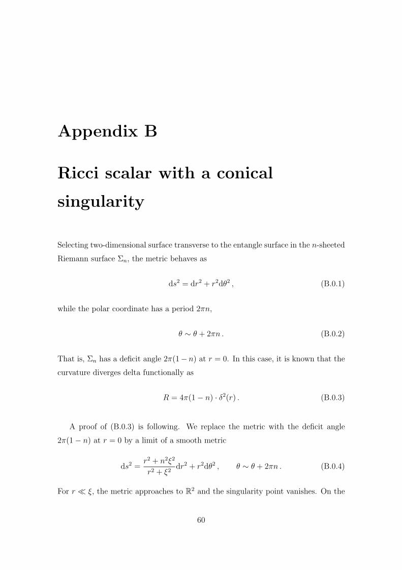
Appendix B

Ricci scalar with a conical

singularity

Selecting two-dimensional surface transverse to the entangle surface in the n-sheeted

Riemann surface Σn, the metric behaves as

ds2 = dr2 + r2dθ2 , (B.0.1)

while the polar coordinate has a period 2πn,

θ ∼ θ + 2πn . (B.0.2)

That is, Σn has a deficit angle 2π(1− n) at r = 0. In this case, it is known that the

curvature diverges delta functionally as

R = 4π(1− n) · δ2(r) . (B.0.3)

A proof of (B.0.3) is following. We replace the metric with the deficit angle

2π(1− n) at r = 0 by a limit of a smooth metric

ds2 =r2 + n2ξ2

r2 + ξ2dr2 + r2dθ2 , θ ∼ θ + 2πn . (B.0.4)

For r ≪ ξ, the metric approaches to R2 and the singularity point vanishes. On the

60

other hand, for r ≫ ξ, the metric (B.0.4) approaches to (B.0.1). It is expected that

the metric (B.0.4) approaches to (B.0.1) under the limit ξ → 0. By using the metric

(B.0.4), the integrand of the curvature gives the value independent on ξ,∫d2r√gR = 4π(1− n) . (B.0.5)

Then, we obtain the relation (B.0.3).

61

Bibliography

[1] Y. Sato, “Comments on entanglement entropy in the dS/CFT correspondence,”

Phys. Rev. D 91 (2015) 8, 086009 [arXiv:1501.04903 [hep-th]].

[2] Y. Sato, work in progress.

[3] Y. Sato and K. Yoshida, “Holographic description of the Schwinger effect in

electric and magnetic fields,” JHEP 1304 (2013) 111 [arXiv:1303.0112 [hep-

th]].

[4] Y. Sato and K. Yoshida, “Potential Analysis in Holographic Schwinger Effect,”

JHEP 1308 (2013) 002 [arXiv:1304.7917 [hep-th]].

[5] Y. Sato and K. Yoshida, “Holographic Schwinger effect in confining phase,”

JHEP 1309 (2013) 134 [arXiv:1306.5512 [hep-th]].

[6] Y. Sato and K. Yoshida, “Universal aspects of holographic Schwinger effect in

general backgrounds,” JHEP 1312 (2013) 051 [arXiv:1309.4629 [hep-th]].

[7] D. Kawai, Y. Sato and K. Yoshida, “Schwinger pair production rate in confining

theories via holography,” Phys. Rev. D 89 (2014) 10, 101901 [arXiv:1312.4341

[hep-th]].

[8] D. Kawai, Y. Sato and K. Yoshida, “A holographic description of the Schwinger

effect in a confining gauge theory,” Int. J. Mod. Phys. A 30 (2015) 11, 1530026

[arXiv:1504.00459 [hep-th]].

[9] J. D. Bekenstein, “Black holes and entropy,” Phys. Rev. D 7 (1973) 2333.

[10] S. W. Hawking, “Particle Creation by Black Holes,” Commun. Math. Phys. 43

(1975) 199 [Commun. Math. Phys. 46 (1976) 206].

62

[11] J. M. Bardeen, B. Carter and S. W. Hawking, “The Four laws of black hole

mechanics,” Commun. Math. Phys. 31 (1973) 161.

[12] G. ’t Hooft, “Dimensional reduction in quantum gravity,” Salamfest 1993:0284-

296 [gr-qc/9310026].

[13] L. Susskind, “The World as a hologram,” J. Math. Phys. 36 (1995) 6377

doi:10.1063/1.531249 [hep-th/9409089].

[14] J. M. Maldacena, “The large N limit of superconformal field theories and su-

pergravity,” Adv. Theor. Math. Phys. 2 (1998) 231 [Int. J. Theor. Phys. 38

(1999) 1113]. [arXiv:hep-th/9711200].

[15] S. S. Gubser, I. R. Klebanov and A. M. Polyakov, “Gauge theory correla-

tors from non-critical string theory,” Phys. Lett. B 428 (1998) 105 [arXiv:hep-

th/9802109].

[16] E. Witten, “Anti-de Sitter space and holography,” Adv. Theor. Math. Phys. 2

(1998) 253 [arXiv:hep-th/9802150].

[17] S. Ryu and T. Takayanagi, “Holographic derivation of entanglement entropy

from AdS/CFT,” Phys. Rev. Lett. 96 (2006) 181602 [hep-th/0603001].

[18] S. Ryu and T. Takayanagi, “Aspects of Holographic Entanglement Entropy,”

JHEP 0608 (2006) 045 [hep-th/0605073].

[19] V. E. Hubeny, M. Rangamani and T. Takayanagi, “A Covariant holographic

entanglement entropy proposal,” JHEP 0707 (2007) 062 [arXiv:0705.0016 [hep-

th]].

[20] B. Swingle, “Entanglement Renormalization and Holography,” Phys. Rev. D

86 (2012) 065007 [arXiv:0905.1317].

[21] M. Van Raamsdonk, “Comments on quantum gravity and entanglement,”

arXiv:0907.2939 [hep-th].

63

[22] M. Nozaki, T. Numasawa, A. Prudenziati and T. Takayanagi, “Dynamics of

Entanglement Entropy from Einstein Equation,” Phys. Rev. D 88 (2013) 2,

026012 [arXiv:1304.7100 [hep-th]].

[23] N. Lashkari, M. B. McDermott and M. Van Raamsdonk, “Gravitational

dynamics from entanglement ’thermodynamics’,” JHEP 1404 (2014) 195

[arXiv:1308.3716 [hep-th]].

[24] M. Nozaki, S. Ryu and T. Takayanagi, “Holographic Geometry of Entangle-

ment Renormalization in Quantum Field Theories,” JHEP 1210 (2012) 193

[arXiv:1208.3469 [hep-th]].

[25] E. Witten, “Quantum gravity in de Sitter space,” hep-th/0106109.

[26] A. Strominger, “The dS / CFT correspondence,” JHEP 0110 (2001) 034 [hep-

th/0106113].

[27] J. M. Maldacena, “Non-Gaussian features of primordial fluctuations in single

field inflationary models,” JHEP 0305 (2003) 013 [astro-ph/0210603].

[28] I. R. Klebanov and A. M. Polyakov, “AdS dual of the critical O(N) vector

model,” Phys. Lett. B 550 (2002) 213 [hep-th/0210114].

[29] S. Giombi and X. Yin, “Higher Spin Gauge Theory and Holography: The

Three-Point Functions,” JHEP 1009 (2010) 115 doi:10.1007/JHEP09(2010)115

[arXiv:0912.3462 [hep-th]].

[30] D. Anninos, T. Hartman and A. Strominger, “Higher Spin Realization of the

dS/CFT Correspondence,” arXiv:1108.5735 [hep-th].

[31] D. Anninos, “De Sitter Musings,” Int. J. Mod. Phys. A 27 (2012) 1230013

[arXiv:1205.3855 [hep-th]].

[32] J. M. Maldacena and C. Nunez, “Supergravity description of field theories on

curved manifolds and a no go theorem,” Int. J. Mod. Phys. A 16 (2001) 822

[hep-th/0007018].

64

[33] D. Kutasov, T. Maxfield, I. Melnikov and S. Sethi, “Constraining de

Sitter Space in String Theory,” Phys. Rev. Lett. 115 (2015) 7, 071305

[arXiv:1504.00056 [hep-th]].

[34] L. Dyson, J. Lindesay and L. Susskind, “Is there really a de Sitter/CFT dual-

ity?,” JHEP 0208 (2002) 045 [hep-th/0202163].

[35] M. Spradlin, A. Strominger and A. Volovich, “Les Houches lectures on de Sitter

space,” hep-th/0110007.

[36] J. D. Brown and M. Henneaux, “Central Charges in the Canonical Realization

of Asymptotic Symmetries: An Example from Three-Dimensional Gravity,”

Commun. Math. Phys. 104 (1986) 207.

[37] D. Klemm, “Some aspects of the de Sitter / CFT correspondence,” Nucl. Phys.

B 625 (2002) 295 [hep-th/0106247].

[38] R. Bousso, A. Maloney and A. Strominger, “Conformal vacua and entropy in

de Sitter space,” Phys. Rev. D 65 (2002) 104039 [hep-th/0112218].

[39] M. Spradlin and A. Volovich, “Vacuum states and the S matrix in dS / CFT,”

Phys. Rev. D 65 (2002) 104037 [hep-th/0112223].

[40] C. M. Hull, “Timelike T duality, de Sitter space, large N gauge theories and

topological field theory,” JHEP 9807 (1998) 021 [hep-th/9806146].

[41] C. M. Hull and R. R. Khuri, “World volume theories, holography, duality and

time,” Nucl. Phys. B 575 (2000) 231 [hep-th/9911082].

[42] A. Strominger, “Inflation and the dS / CFT correspondence,” JHEP 0111

(2001) 049 [hep-th/0110087].

[43] P. McFadden and K. Skenderis, “Holography for Cosmology,” Phys. Rev. D 81

(2010) 021301 [arXiv:0907.5542 [hep-th]].

[44] P. McFadden and K. Skenderis, “The Holographic Universe,” J. Phys. Conf.

Ser. 222 (2010) 012007 [arXiv:1001.2007 [hep-th]].

65

[45] M. A. Vasiliev, “Consistent equation for interacting gauge fields of all spins in

(3+1)-dimensions,” Phys. Lett. B 243 (1990) 378.

[46] A. LeClair and M. Neubert, “Semi-Lorentz invariance, unitarity, and crit-

ical exponents of symplectic fermion models,” JHEP 0710 (2007) 027

[arXiv:0705.4657 [hep-th]].

[47] D. J. Robinson, E. Kapit and A. LeClair, “Lorentz Symmetric Quantum

Field Theory for Symplectic Fermions,” J. Math. Phys. 50 (2009) 112301

[arXiv:0903.2399 [hep-th]].

[48] G. S. Ng and A. Strominger, “State/Operator Correspondence in Higher-Spin

dS/CFT,” Class. Quant. Grav. 30 (2013) 104002 [arXiv:1204.1057 [hep-th]].

[49] C. M. Chang, A. Pathak and A. Strominger, “Non-Minimal Higher-Spin

DS4/CFT3,” arXiv:1309.7413 [hep-th].

[50] P. Ouyang, “Toward Higher Spin dS3/CFT2,” arXiv:1111.0276 [hep-th].

[51] C. Krishnan and S. Roy, “Higher Spin Resolution of a Toy Big Bang,” Phys.

Rev. D 88 (2013) 044049 [arXiv:1305.1277 [hep-th]].

[52] C. Krishnan, A. Raju, S. Roy and S. Thakur, “Higher Spin Cosmology,” Phys.

Rev. D 89 (2014) 4, 045007 [arXiv:1308.6741 [hep-th]].

[53] P. Calabrese and J. L. Cardy, “Entanglement entropy and quantum field the-

ory,” J. Stat. Mech. 0406 (2004) P06002 [hep-th/0405152].

[54] H. Casini and M. Huerta, “Entanglement entropy in free quantum field theory,”

J. Phys. A 42 (2009) 504007 [arXiv:0905.2562 [hep-th]].

[55] A. Lewkowycz and J. Maldacena, “Generalized gravitational entropy,” JHEP

1308 (2013) 090 [arXiv:1304.4926 [hep-th]].

[56] S. Fischetti and D. Marolf, “Complex Entangling Surfaces for AdS and Lifshitz

Black Holes?,” Class. Quant. Grav. 31 (2014) 21, 214005 [arXiv:1407.2900 [hep-

th]].

66

[57] K. Narayan, “Extremal surfaces in de Sitter spacetime,” Phys. Rev. D 91 (2015)

12, 126011 [arXiv:1501.03019 [hep-th]].

[58] K. Narayan, “de Sitter space and extremal surfaces for spheres,” Phys. Lett. B

753 (2015) 308. [arXiv:1504.07430 [hep-th]].

[59] M. Ammon, A. Castro and N. Iqbal, “Wilson Lines and Entanglement Entropy

in Higher Spin Gravity,” JHEP 1310 (2013) 110 [arXiv:1306.4338 [hep-th]].

[60] J. de Boer and J. I. Jottar, “Entanglement Entropy and Higher Spin Holography

in AdS3,” JHEP 1404 (2014) 089 [arXiv:1306.4347 [hep-th]].

67