iieej transactions on image electronics and image

IIEEJ Transactions on Image Electronics and Visual Computing

IIEEJ Transactions on

Image Electronics and

Visual Computing

I.I.E.E.JVol. 8, No. 1 2020

Special Issue on Extended Papers Presented in IEVC2019

Editorial Committee of IIEEJ

Editor in Chief Mei KODAMA (Hiroshima University)

Vice Editors in Chief Osamu UCHIDA (Tokai University) Naoki KOBAYASHI (Saitama Medical University) Yuriko TAKESHIMA (Tokyo University of Technology)

Advisory Board Yasuhiko YASUDA (Waseda University Emeritus) Hideyoshi TOMINAGA (Waseda University Emeritus) Kazumi KOMIYA (Kanagawa Institute of Technology) Fumitaka ONO (Tokyo Polytechnic University Emeritus) Yoshinori HATORI (Tokyo Institute of Technology) Mitsuji MATSUMOTO (Waseda University Emeritus) Kiyoshi TANAKA (Shinshu University) Shigeo KATO (Utsunomiya University Emeritus)

Editors Yoshinori ARAI (Tokyo Polytechnic University) Chee Seng CHAN (University of Malaya) Naiwala P. CHANDRASIRI (Kogakuin University) Chinthaka PREMACHANDRA (Shibaura Institute of Technology) Makoto FUJISAWA(University of Tsukuba) Issei FUJISHIRO (Keio University) Kazuhiko HAMAMOTO (Tokai University) Madoka HASEGAWA (Utsunomiya University) Ryosuke HIGASHIKATA (Fuji Xerox Co., Ltd.) Naoto KAWAMURA (Canon OB) Shunichi KIMURA (Fuji Xerox Co., Ltd.) Shoji KURAKAKE (NTT DOCOMO) Takashi KANAI (The University of Tokyo) Tetsuro KUGE (NHK Engineering System, Inc.) Koji MAKITA (Canon Inc.) Junichi MATSUNOSHITA (Fuji Xerox Co., Ltd.) Tomoaki MORIYA (Tokyo Denki University) Paramesran RAVEENDRAN (University of Malaya) Kaisei SAKURAI (DWANGO Co., Ltd.) Koki SATO (Shonan Institute of Technology) Kazuma SHINODA (Utsunomiya University) Mikio SHINYA (Toho University) Shinichi SHIRAKAWA (Aoyama Gakuin University) Kenichi TANAKA (Nagasaki Institute of Applied Science) Yukihiro TSUBOSHITA (Fuji Xerox Co., Ltd.) Daisuke TSUDA (Shinshu University) Masahiro TOYOURA (University of Yamanashi) Kazutake UEHIRA (Kanagawa Institute of Technology) Yuichiro YAMADA (Genesis Commerce Co.,Ltd.) Norimasa YOSHIDA (Nihon University) Toshihiko WAKAHARA (Fukuoka Institute of Technology OB) Kok Sheik WONG (Monash University Malaysia)

Reviewer Hernan AGUIRRE (Shinshu University) Kenichi ARAKAWA (NTT Advanced Technology Corporation) Shoichi ARAKI (Panasonic Corporation) Tomohiko ARIKAWA (NTT Electronics Corporation) Yue BAO (Tokyo City University) Nordin BIN RAMLI (MIMOS Berhad) Yoong Choon CHANG (Multimedia University) Robin Bing-Yu CHEN (National Taiwan University) Kiyonari FUKUE (Tokai University) Mochamad HARIADI (Sepuluh Nopember Institute of Technology) Masaki HAYASHI (UPPSALA University) Takahiro HONGU (NEC Engineering Ltd.) Yuukou HORITA (University of Toyama) Takayuki ITO (Ochanomizu University) Masahiro IWAHASHI (Nagaoka University of Technology) Munetoshi IWAKIRI (National Defense Academy of Japan)

Yuki IGARASHI (Meiji University) Kazuto KAMIKURA (Tokyo Polytechnic University) Yoshihiro KANAMORI (University of Tsukuba) Shun-ichi KANEKO (Hokkaido University) Yousun KANG (Tokyo Polytechnic University) Pizzanu KANONGCHAIYOS (Chulalongkorn University) Hidetoshi KATSUMA (Tama Art University OB) Masaki KITAGO (Canon Inc.) Akiyuki KODATE (Tsuda College) Hideki KOMAGATA (Saitama Medical University) Yushi KOMACHI (Kokushikan University) Toshihiro KOMMA (Tokyo Metropolitan University) Tsuneya KURIHARA (Hitachi, Ltd.) Toshiharu KUROSAWA (Matsushita Electric Industrial Co., Ltd. OB) Kazufumi KANEDA (Hiroshima University) Itaru KANEKO (Tokyo Polytechnic University) Teck Chaw LING (University of Malaya) Chu Kiong LOO (University of Malaya) Xiaoyang MAO (University of Yamanashi) Koichi MATSUDA (Iwate Prefectural University) Makoto MATSUKI (NTT Quaris Corporation OB) Takeshi MITA (Toshiba Corporation) Hideki MITSUMINE (NHK Science & Technology Research Laboratories) Shigeo MORISHIMA (Waseda University) Kouichi MUTSUURA (Shinsyu University) Yasuhiro NAKAMURA (National Defense Academy of Japan) Kazuhiro NOTOMI (Kanagawa Institute of Technology) Takao ONOYE (Osaka University) Hidefumi OSAWA (Canon Inc.) Keat Keong PHANG (University of Malaya) Fumihiko SAITO (Gifu University) Takafumi SAITO (Tokyo University of Agriculture and Technology) Tsuyoshi SAITO (Tokyo Institute of Technology) Machiko SATO (Tokyo Polytechnic University Emeritus) Takayoshi SEMASA (Mitsubishi Electric Corp. OB) Kaoru SEZAKI (The University of Tokyo) Jun SHIMAMURA (NTT) Tomoyoshi SHIMOBABA (Chiba University) Katsuyuki SHINOHARA (Kogakuin University) Keiichiro SHIRAI (Shinshu University) Eiji SUGISAKI (N-Design Inc. (Japan), DawnPurple Inc.(Philippines)) Kunihiko TAKANO (Tokyo Metropolitan College of Industrial Technology) Yoshiki TANAKA (Chukyo Medical Corporation) Youichi TAKASHIMA (NTT) Tokiichiro TAKAHASHI (Tokyo Denki University) Yukinobu TANIGUCHI (NTT) Nobuji TETSUTANI (Tokyo Denki University) Hiroyuki TSUJI (Kanagawa Institute of Technology) Hiroko YABUSHITA (NTT) Masahiro YANAGIHARA (KDDI R&D Laboratories) Ryuji YAMAZAKI (Panasonic Corporation)

IIEEJ Office Osamu UKIGAYA Rieko FUKUSHIMA Kyoko HONDA

Contact Information The Institute of Image Electronics Engineers of Japan (IIEEJ） 3-35-4-101, Arakawa, Arakawa-ku, Tokyo 116-0002, Japan Tel : +81-3-5615-2893 Fax : +81-3-5615-2894 E-mail : [email protected] http://www.iieej.org/ (in Japanese) http://www.iieej.org/en/ (in English) http://www.facebook.com/IIEEJ (in Japanese) http://www.facebook.com/IIEEJ.E (in English)

1 Upon the Special Issue on Extended Papers Presented in IEVC2019 Naoki KOBAYASHI

2 Technique to Embed Information in 3D Printed Objects Using Near Infrared

Fluorescent Dye

Hideo KASUGA, Piyarat SILAPASUPHAKORNWONG,

Hideyuki TORII, Masahiro SUZUKI, Kazutake UEHIRA

10 Feasibility Study of Deep Learning Based Japanese Cursive Character

Recognition

Kazuya UEKI, Tomoka KOJIMA

17 Elastic and Collagen Fibers Segmentation Based on U-Net Deep Learning

Using Hematoxylin and Eosin Stained Hyperspectral Images

Lina SEPTIANA, Hiroyuki SUZUKI, Masahiro ISHIKAWA,

Takashi OBI, Naoki KOBAYASHI, Nagaaki OHYAMA,

Takaya ICHIMURA, Atsushi SASAKI, Erning WIHARDJO,

Harry ARJADI

27 Pressure Sensitivity Pattern Analysis Using Machine Learning Methods Henry FERN´ANDEZ, Koji MIKAMI, Kunio KONDO

35 Image Completion of 360-Degree Images by cGAN with Residual Multi-Scale

Dilated Convolution

Naofumi AKIMOTO, Yoshimitsu AOKI

Regular Section

44 Multi-Class Dictionary Design Algorithm Based on Iterative Class Update K-

SVD for Image Compression

Ji WANG, Yukihiro BANDOH, Atsushi SHIMIZU,

Yoshiyuki YASHIMA

58 A Configurable Fixed-Complexity IME-FME Cost Ratio Based Inter Mode

Filtering Method in HEVC Encoding

Muchen LI, Jinjia ZHOU, Satoshi GOTO

Announcements

71 Call for Papers: Special Issue on Image-Related Technologies for the

Realization of Future Society

72 Call for Papers: ITU KALEIDOSCOPE 2020

Guide for Authors

75 Guidance for Paper Submission

3-35-4-101，Arakawa，Arakawa-ku，Tokyo 116-0002，Japan

Tel：+81-5615-2893　Fax：+81-5615-2894　E-mail：[email protected]　http://www.iieej.org/

　　　　　　　　　　　　　　　　　　　　IIEEJ Transactions on

　　　　　　 Image Electronics and Visual Computing

　　　Vol.8 No.1 　June 2020

　　CONTENTS

Published two times a year by the Institute of Image Electronics Engineers of Japan（IIEEJ）

Contributed Papers

Contributed Papers

Special Issue on Extended Papers Presented in IEVC2019

Upon the Special Issue on

Extended Papers Presented in IEVC2019

Editor: Prof. Naoki KOBAYASHI

Saitama Medical University

The Institute of Image Electronics Engineering of Japan (IIEEJ) regularly holds

International academic events named “Image Electronics and Visual Computing (IEVC)”

since 2007, on every two or two and half years. The 6th International Conference on Image

Electronics and Visual Computing (IEVC2019) was held in Bali, Indonesia on August 21-24,

2019．From this time, the name of this event was changed from International Workshop to

International Conference to promote the event more worldwide and more attractive for

speakers and attendees. The conference was successfully held with 109 presentations and 165

participants (including 39 foreigners from more than 10 countries).

There were two paper categories in IEVC2019: general paper and late breaking paper

(LBP), and in general paper, there were two tracks: Journal track (JT) and Conference

track (CT). In IEVC2019, 33 JT papers, 52 CT papers and 24 LBP were submitted.

Journal track is a newly introduced one and has the advantage to be able to publish the

paper on the journal (IIEEJ Trans. on IEVC) in the “Special Issue on Journal Track in

IEVC2019” on December 2019 issue, by submitting full paper version (8 pages) together

with conference paper version to be peer-reviewed in advance. Actually seven papers were

adopted in the “Special Issue on Journal Track in IEVC2019” published on December 2019.

The special issue on “Extended Papers Presented in IEVC2019” to be published on June

2020 was openly called for all paper categories in IEVC2019, and five papers have passed

the review process to be in time for its publishing schedule. In them, the JT papers not to be

in time for the publication of December 2019 Special issue are also included. The papers

currently under review will be published in the next issue, if accepted.

Finally, I would like to give great thanks to all the reviewers and editors for their time

and efforts towards improving the quality of papers. I would also like to express my

deepest appreciation to the editorial committee members of IIEEJ and the staff at IIEEJ

office for various kinds of support.

IIEEJ Transactions on Image Electronics and Visual Computing Vol.8 No.1 （2020）

1

Technique to Embed Information in 3D Printed Objects Using Near Infrared

Fluorescent Dye

Hideo KASUGA† (Member), Piyarat SILAPASUPHAKORNWONG†, Hideyuki TORII†, Masahiro SUZUKI††,

Kazutake UEHIRA† (Member)

†Kanagawa Institute of Technology, ††Tokiwa University

<Summary> This paper presents a new technique to embed information in 3D printed objects using a near infrared

fluorescent dye. Regions containing a small amount of fluorescent dye are formed inside an object during fabrication to embed

information inside it, and these regions form a pattern that expresses certain information. When this object is irradiated with

near-infrared rays, they pass through the object made of resin but are partly absorbed by the fluorescent dye in the pattern

regions, and it emits near-infrared fluorescence. Therefore, the internal pattern can be captured as a high-contrast image using a

near-infrared camera, and the embedded information can be nondestructively read out. This paper presents a technique of

forming internal patterns at two different depths to double the amount of embedded information. We can determine the depth of

the pattern from the image because the distribution of the brightness of the captured image of the pattern depends on its depth.

We can also know from the brightness distribution whether or not a pattern exists at two depths. Because this can express four

states, the amount of embedded information can be doubled using this method. We conducted experiments using deep learning

to distinguish four states from the captured image. The experiments demonstrated the feasibility of this technique by showing

that accurate embedded information can be read out.

Keywords: 3D printer, digital fabrication, information embedding, deep learning

1. Introduction

Digital fabrication has been attracting attention as a new

method of manufacturing. This is because a user can obtain

a product that he or she wants just by inputting the model

data into fabrication equipment. If a user has equipment at

home or in the office, he or she can easily obtain a product

by obtaining the model data through the Internet and print it.

3D printers are typical digital fabrication equipment that has

been reduced in price and miniaturized. As a result, they are

beginning to become popular with consumers. Thus, 3D

printers are expected to revolutionize distribution and

manufacturing in the future1-3).

3D printers use a unique process called additive

manufacturing in which thin layers are formed one by one to

form an object4). This enables forming any structure inside

the object during fabrication. We have studied techniques

that form fine patterns inside the object to express

information5-9). These patterns are made invisible from the

outside. Therefore, information can be embedded in the

object so that it cannot be seen.

The embedding of information inside 3D printed objects

will enable extra value to be added to these objects,

expanding their applications. For example, we can embed

information that usually comes with newly purchased

products (e.g., user manuals) into them. Moreover, it will be

possible to use them as “things” of the Internet of Things

(IoT) in connecting to the Internet.

In addition to embedding information, we have also

studied techniques that can read out embedded information

nondestructively from the outside. In that study, we used a

fused deposition modeling (FDM) 3D printer with resin as a

material. We have studied some techniques to read out

embedded information, and one of them uses a near infrared

camera. We formed fine patterns inside the fabricated

objects using resin that has a high reflectivity or high

absorption rate for near infrared light. Those resins were

basically the same kind as that of the body of the object. We

could capture the inside pattern using a near infrared camera

because most resin materials transmit near infrared rays.

We have also studied a technique for forming patterns

containing a small amount of fluorescent dye. Fluorescent

dye emits near-infrared fluorescence; therefore, the internal

pattern can be captured as a high-contrast image using a

near-infrared camera. This enhances the readability of the

embedded information.

　　-- Special Issue on Extended Papers Presented in IEVC2019 --


2

This paper describes a technique that can double the

amount of information embedded. It embeds patterns

containing fluorescent dye at two different depths to achieve

double the amount of embedded information. In order to

read out information, we needed a technique to recognize

whether or not a pattern exists at each depth. We used deep

learning for this recognition. This paper also describes the

results of experiments conducted to validate the feasibility of

this method.

2. Information Embedding Inside 3D Printed

Objects

2.1 Information embedding by forming fine patterns

inside 3D printed objects

Figure 1 illustrates a simple example of embedding

information inside an object by forming fine patterns. A

3D-printed object contains fine domains having physical

characteristics such as optical, acoustic, or heat conduction

differing from the other part of the object. Although various

ways can be used to express information due to the

disposition of the fine domain, one example involves binary

data, “1” or “0,” being expressed due to a fine domain

existing or not existing in a designated position, as shown in

Fig. 1.

We can expect to read out these embedded binary data

by detecting the presence or absence of a domain at a

designated position utilizing the difference in physical

characteristics between the materials of the fine domain and

another part of the object.

In our previous study, inside patterns were sensed

nondestructively from outside the object using a near

infrared camera and thermography to determine the

difference in the thermal conductivity and optical

characteristics in a near infrared region.

2.2 Related work on Information embedding inside 3D

printed objects

Related work includes a technique of embedding

information inside 3D printed objects using a thin plate with

a cutout pattern. Willis and Wilson first created product

parts, one of which had a visible pattern, and then assembled

these parts into one product so that the patterned part was

inside it10). They read out the patterned information inside

using terahertz wavelength light. However, in practical

terms, applying it to common 3D printing was too

complicated.

Another related study involved embedding an RFID tag

in 3D printed objects11). Object fabrication is suspended

once in embedding an RFID tag, and it is put on the

fabricated surface; then, fabrication is resumed to cover the

RFID tag. After fabrication is completed, the RFID tag is

embedded inside the objects.

In these related studies, users could not make an object

by just inputting data. They needed additional parts and

additional processes; therefore, the features of 3D printing

were completely lost. In contrast, the patterns in our

technique are integrally formed using the body-utilizing

additive manufacturing process of 3D printers, which

eliminates any additional processes. This means whoever

obtains data can make the objects in which information is

embedded inside.

2.3 Information embedding using fluorescent dye

Figure 2 shows the basic principle of the technique using

fluorescent dye. It assumes that the resin is used as an object

material. The dotted rectangles in Fig. 2 indicate the inside

pattern region. The pattern regions are formed using the

same resin as that of the other regions, but they contain a

small amount of fluorescent dye. The rays reach the internal

fluorescent dye when the object is irradiated with

near-infrared rays from the outside because resin has high

transmittance for near infrared. The light source irradiates

Fig. 1 Example of embedding information inside object

Fabricated object

1 1 0 1 0 1 1

Inside pattern

Near infrared light source

3D Printed object

Inside pattern

Near infrared light with wavelength L

from light source

Near infrared light with wavelength F emitted by fluorescent dye

Fig. 2 Basic concept of technique

Near infrared light camera

Optical filter


3

light with wavelength λL in the near infrared region, which

excites the fluorescent dye. The dye is excited and emits

florescence with wavelength λF, which is also near the

infrared region but differs from λL. Because the dye emits

the light, a bright image of the patterns inside the resin

object can be captured.

Because wavelength λF of the dye's fluorescence differs

from wavelength λL of the irradiated light, only light the

fluorescent dye emits enters the camera. An optical filter that

blocks the source light reflected from the object surface is

used; therefore, a low noise image of the inside patterns can

be obtained.

2.4 Dual depth embedding

Figure 3 shows the basic configuration of dual depth

embedding. The inside patterns are formed at two different

depths. We can express 2-bit information at one position

using this arrangement. For example, we can assign (11)

when patterns exist at both depths (A in Fig. 3), (10) when a

pattern exists at only low depth (B in Fig. 3), (01) when it is

at only high depth (C in Fig. 3), and (00) when no pattern

exists (D in Fig. 3). In the previous method, only one bit

could be embedded at one position, but this method enables

embedding two bits. Therefore, the amount of information

that can be embedded is double.

Near-infrared rays transmit through the resin but are

scattered to some extent during transmission. This scattering

increases as the passing distance increases. Therefore, when

the near infrared image of the internal pattern is captured

from the outside, the image of the pattern blurs. In addition,

the blurring becomes more pronounced for images of deep

patterns. Therefore, the brightness distribution of the

captured image changes depending on the depth, as shown

in Fig. 3. The difference in the brightness distribution at

positions B and C in Fig. 3 shows this state clearly. When

patterns are at two depths, the brightness distribution is the

sum of them, as shown in Fig. 3, for position A. Therefore,

we should be able to recognize which of the four cases the

captured image is; that is, 2-bit binary information can be

read out.

In our previous study12), we could see clear differences

in brightness distribution at four positions, as shown in Fig.

3, for the naked eye–except between images at Position A

and Position B.

Recognizing these four states using pattern recognition

techniques is possible because few differences are evident in

the histogram of the captured image for (11) and (10) and

because few differences are evident in the brightness

distribution. In this study, we used deep learning to

recognize the four states and read out the 2-bit binary

information from each position.

3. Experiments

3.1 Sample preparation

Figure 4 shows the designed layout of the sample. Four

types of arrangements of patterns at two depths were formed

in equal numbers for each row. The pattern size was 1×1

mm, and the thickness was 1 mm. The reason for adopting

1×1 mm as the minimum size was that this pattern was the

smallest that could be formed stably.

The depth of the upper pattern from the surface was 0.5

Bri

ghtn

ess

Inside pattern

Fig. 3 Basic configuration of dual depth

Cross section of 3D printed object

A (11)

B (10)

C (01)

D (00)

Fig. 4 Layout of sample

(b) Cross section

(a) Top views

2 mm

0.5 mm 1.0 mm

4.3 mm

3 mm

Inside pattern

2.0 mm 1.0 mm


4

mm, and that of the bottom pattern was 2 mm. The reason

for setting the depth to 0.5 mm was that the pattern could not

be seen from the outside at that depth. As the bottom pattern

becomes deeper, the blurring of the pattern increases, and it

becomes easier to distinguish from the shallow pattern.

However, if it becomes too deep, the brightness decreases

significantly, and the pattern cannot be recognized.

Therefore, we chose 2 mm as the optimum depth for the

bottom pattern.

We used a FDM 3D printer, Mutoh Value3D MagiX

2200D, shown in Fig. 5, to fabricate the samples. It has two

nozzles so that two kinds of materials can be used for one

object. The lamination pitch (resolution in the z-direction) of

this 3D printer was 0.05 mm.

The body structure was fabricated using pure

acrylonitrile butadiene styrene (ABS) resin, which is the one

on the right in Fig. 5, and the inside patterns were formed

using the same ABS resin as that for the body; however, it

contained a small amount of florescent dye (less than 1%),

which can be seen on the left. The color of the ABS

containing florescent dye is almost the same as that of pure

ABS. Therefore, even if the pattern is formed very shallow

from the surface, it cannot be seen.

The melting temperature of the ABS containing

fluorescent dye was the same as that of pure ABS; therefore,

the sample was fabricated in a successive process using the

same temperature for the nozzle and stage. Figure 6 shows

an example of the samples.

3.2 Capture of near infrared images

Figure 7 shows the layout and photograph of the near

infrared image capture system used to take a near infrared

Image. We used two sets of LED arrays as near infrared

light sources. They were placed 10 cm away from the

sample. Their wavelength was 760 nm, and the power was

12 W in a total of 2 sets. A 2048 × 1088 pixel CCD camera,

a conventional silicon-based one, was used. Because we

removed the cold filter placed in front of the CCD sensor, it

was sensitive to light with wavelengths up to 1100 nm. It

was set at the same side as the aforementioned sample

between the LED arrays.

An optical filter was placed in front of the camera lens.

We used a long-pass optical filter with a cutoff wavelength

of 850 nm.

3.3 Reading out embedded information using deep

learning

Four kinds of neural network, ResNet5013), Network in

ABS containing florescent dyePure ABS

Fig. 5 3D printer used in experiment

Fig. 7 Near infrared image capture

LED array

Sample

LED array

Near infrared CCD camera Optical filter

Fig. 6 An example of samples.

Near infrared CCD camera

Optical filter

LED arrays

Sample

(a) Layout

(b) Photograph


5

Network (NIN) 14), GoogLeNet15), and an original model

were used to distinguish four states of captured images for

reading out embedded information. ResNet50, NIN, and

GoogLeNet are neural networks commonly used in the field

of image classification. In our study, these neural networks

consisted of the same network used in ImageNet large scale

visual recognition challenge (ILSVRC).

The original model is a simple but highly accurate neural

network. It is based on VGG16), and the number of layers

and the number of channels were adjusted. The

configuration is shown in Fig. 8. The layers are shown in

Table 1. The input to our original network is a 108× 08 grayscale

image. Therefore, the size of the first convolution layer is 108×108

× 16. We used a 3× convolution filter. The convolution stride is 1.

ReLU was used for the activation function. The number of channels

in the first layer is 16 because the accuracy did not improve and

because the calculation cost increased even if the number of

channels was very high. Max pooling was performed with a kernel

size of 2× 2 and a stride of 2. As a result, the spatial resolution was

down-sampled in half. The number of channels was doubled after

each max pooling layer. However, the last two convolution layers

had 512 channels. This is because increasing the number of

channels in the last two layers improved accuracy. The global

average pooling layer, the fully connected layer, and the soft-max

layer come after the convolution layers.

Images at each position with 108×108 pixels were cut

out. These images were input to neural networks. Because

the sample had only six positions for each binary number, as

shown in Fig. 3, 25 photos of the sample were taken under

various conditions. Therefore, 150 photos were obtained for

each binary number, that is, 600 photos were used in the

evaluation. 500 photos were used for training, and 100

photos were used for the evaluation. We evaluated the

accuracy in reading out embedded information using the

aforementioned deep learning.

4. Results and Discussion

Figure 9 shows one example of images of the sample

Fig. 8 Configuration of original neural network model

Input image 108 x 108 x 1

Convolution 108 x 108 x 16


Max pooling



Max pooling



Max pooling



Max pooling



Max pooling

Global average pooling

Fully connected 4

Softmax

Table 1 Layers of original model

108 x 108 x 16

54 x 54 x 32

27 x 27 x 64

13 x 13 x 128 6 x 6 x 512

Convolution

Max pooling

Global average pooling

Fully connected

Softmax

Input 108 x 108 x 1

Fig. 9 Example image of the sample captured with near

infrared CCD camera

Fig. 10 Example images cut out at position shown in Fig. 3

(a) Position A (b) Position B

(c) Position C (d) Position D


6

captured with the CCD camera, and Fig. 10 shows the example

images cut out at a position shown in Fig. 3 as A to D. Figure

10 (b) and (c) show that the blur of the image differs depending

on the depth of the pattern, as expected. Therefore, the three

cases having only one pattern or no pattern at two depths can be

distinguished from each other using the distribution. However,

no clear difference in the image and the luminance distribution

is evident when only one pattern is at a shallow position and

when two patterns are at both depths. This is because the light

intensity from the pattern at the shallow position is much higher

than that at the deep position. If the depth of the latter pattern

decreases or if the thickness of the pattern is increased, the

difference between the two can be seen.

In order to distinguish four cases, we performed neural

network training using 500 images captured with the CCD

camera. We randomly selected 10% of the training data for

use as validation data. Figure 11 shows the training

accuracy and validation accuracy of four kinds of neural

networks. The training curve indicates that training was

almost completed at 200 epochs in any neural network. The

training accuracy after sufficient training was nearly 100%

for all models. However, the validation accuracy of NIN and

ResNet50 was lower than the training accuracy. In particular,

the training curve of ResNet50 was mostly very high, but

the validation curve was lower in the whole range. These

results indicate that overfitting occurred. Because overfitting

naturally occurs when the model is too complex, ResNet50

was too complex for our study. The original model, which

has a simple structure, had almost no difference between the

training curve and the validation curve. Therefore,

overfitting hardly occurred with it. Because GoogLeNet also

had almost no difference between the training curve and the

validation curve, overfitting hardly occurred with it, as well.

According to these training and validation curves,

GoogLeNet and Original model showed high accuracy.

To evaluate the discrimination accuracy using the

trained model, we conducted a test using 100 images

captured with the CCD camera. These images, which were

test data sets, were randomly selected from 600 images

captured for the experiment. We repeated training and

testing 12 times to find the average of the discrimination

accuracy. Table 2 shows the average accuracies of the test

data set evaluated using the trained models. The accuracy

was over 90% with any neural network. Although the

Training accuracy

Validation accuracy

(c) GoogLeNet

(b) NIN (a) ResNet50

(d) Original model

Fig. 11 Training accuracy and validation accuracy


7

difference in accuracy was small, GoogLeNet was the most

accurate. However, the original model was just as accurate.

Because our model had fewer parameters than GoogLeNet,

it could be calculated faster and required less machine power.

Because the difference in accuracy between GoogLeNet and

Original model was small, the original model was

sufficiently effective. The accuracy of ResNet50 was lower

than that of the original model. ResNet50 had the most

parameters among the four neural networks and took time to

process. NIN is a neural network that was calculated faster

than GoogLeNet or ResNet50, but it had the lowest

accuracy among the four kinds of neural network.

The accuracy rates of these four kinds of neural

networks were all as high as about 95%, though a slight

difference was evident between them. These high accuracies

indicate the possibility of achieving 100% with some

improvement in the future.

We did not reach 100% accuracy in this study for two

reasons. The first was that the difference between the images

of the pattern at positions A and B was too small. This is

because the brightness of the images of deep patterns was

small; therefore, increasing the brightness using the

aforementioned methods will improve the accuracy. The

second reason is that only 500 images were used for learning,

and this was not enough for image recognition by deep

learning. The accuracy will be further improved if the

number of images for learning is increased.

5. Conclusion

We studied a technique to embed information in 3D

printed objects by forming patterns at two depths inside the

object using a near infrared fluorescent dye. The fluorescent

dye was used because it can capture bright, high-contrast

pattern images. This technique can double the amount of

embedded information by expressing 2-bit information

depending on whether or not patterns exist at two depths. In

the experiments, whether or not a pattern existed at each of

the two depths was identified using four kinds of neural

networks from the images taken using a near infrared

camera. Experiment results showed that the accuracy rates

of these four neural networks were all as high as about 95%.

These high accuracies indicate the possibility of achieving

100% with some improvement in the future and indicate the

feasibility of this technique.

In future work, we will optimize the depth and thickness

of the deep patterns to distinguish the four states clearly, in

addition to increasing the number of images used for

learning. This should enable achieving 100% accurate

recognition.

Acknowledgement

We would like to thank DIC Corporation for providing

the fluorescent dye used in this study. This research was

supported by a grant aid program from the Kanagawa

Institute of Technology in 2018.

References

1) B. Berman: “3-D Printing: The New Industrial Revolution”, Business

Horizons, Vol. 55, No. 2, pp. 155–162 (2012).

2) B. Garrett: “3D Printing: New Economic Paradigms and Strategic

Shifts”, Global Policy, Vol. 5, No. 1, pp. 70–75 (2014).

3) C. Weller, R. Kleer, F. T. Piller: “Economic Implications of 3D

Printing: Market Structure Models in Light of Additive Manufacturing

Revisited”, Proc. of International Journal of Production Economics,

Vol. 164, pp. 43–56 (2015).

4) S. Yang, Y. F. Zhao: “Additive Manufacturing-Enabled Design Theory

and Methodology: A Critical Review”, International Journal of

Advanced Manufacturing Technology, Vol. 80, No. 1-4, pp. 327–342

(2015).

5) M. Suzuki, P. Silapasuphakornwong, K. Uehira, H. Unno, Y.

Takashima: “Copyright Protection for 3D Printing by Embedding

Information inside Real Fabricated Objects”, International Conference

on Computer Vision Theory and Applications, pp. 180–185 (2015).

6) M. Suzuki, P. Dechrueng, S. Techavichian, P. Silapasuphakornwong,

H. Torii, K. Uehira: “Embedding Information into Objects Fabricated

With 3-D Printers by Forming Fine Cavities inside Them”, Proc. of

IS&T International symposium on Electronic Imaging, Vol. 2017, No.

41, pp. 6–9 (2017) .

7) P. Silapasuphakornwong, M. Suzuki, H. Unno, H. Torii, K. Uehira, Y.

Takashima: “Nondestructive Readout of Copyright Information

Embedded in Objects Fabricated with 3-D Printers”, Proc. of The 14th

International Workshop on Digital-forensics and Watermarking,

Revised Selected Papers, pp.232–238 (2016).

8) K. Uehira, P. Silapasuphakornwong, M. Suzuki, H. Unno, H. Torii,

Y. Takashima: “Copyright Protection for 3D Printing by Embedding

Information Inside 3D-Printed Object”, Proc. of The 15th International

Workshop on Digital-forensics and Watermarking Revised Selected

Papers, pp.370–378 (2017).

Table 2 Average of discrimination accuracy of each model

Network model Average accuracy

ResNet50 94.25%

NIN 93.67%

GoogLeNet 95.50%

Original model 95.42%


8

9) P. Silapasuphakornwong, M. Suzuki, H. Torii, K. Uehira, Y.

Takashima: “New Technique of Embedding Information inside 3-D

Printed Objects”, Journal of Imaging Science and Technology, Vol. 63,

No. 1, pp. 010501-1- 010501-8 (2019).

10) K. D. D. Willis, A. D. Wilson: “InfraStructs: Fabricating Information

inside Physical Objects for Imaging in the Terahertz Region”, ACM

Trans. on Graphics, Vol. 32, No. 4, pp. 138-1–138-10 (2013.).

11) K. Fujiyoshi: “Personal Fabrication That Links Information with

Things Using RFID Tags”, Keio University Graduation Thesis (2015)

in Japanese.

12) P. Silapasuphakornwong, H. Trii, K. Uehira, A. Funsian, K.

Asawapithulsert, T. Sermpong: “Embedding Information in 3D

Printed Objects Using Double Layered Near Infrared Fluorescent

Dye”, Proc. of 3rd International Conference on Imaging, Signal

Processing and Communication (2019).

13) K. He, X. Zhang, S. Ren, J. Sun: “Deep Residual Learning for Image

Recognition”, Proc. of The IEEE Conference on Computer Vision and

Pattern Recognition (CVPR), pp. 770–778, (2016).

14) M. Lin, Q. Chen, S. Yan: “Network in Network”, arXiv: 1312.4400

(2013).

15) C. Szegedy, W. Liu, Y. Jia, P. Sermanet, S. Reed, D. Anguelov, D.

Erhan, V. Vanhoucke, A. Rabinovich: “Going Deeper with

Convolutions”, Proc. of The IEEE Conference on Computer Vision

and Pattern Recognition, pp. 1–9 (2015).

16) K. Simonyan, A. Zisserman, “Very Deep Convolutional Networks for

Large-Scale Image Recognition”, CoRR, abs/ 1409.1556 (2014).

(Received September 26, 2019)

Hideo KASUGA (Member)

He received his B. E. and M. E. degree in computer science, and his Ph. D. degree in engineering from Shinshu University in 1995, 1997 and 2000, respectively. He is currently an associate professor at the Department of Information Media, Kanagawa Institute of Technology. His research interests include image processing, image recognition and machine learning.

Piyarat SILAPASUPHAKORNWONG

She received her BS (2007) and Ph.D. (2013) in Imaging Science from Chulalongkorn University, Bangkok, Thailand. Since 2014, she has been aresearcher at the Human Media Research Center, Kanagawa Institute of Technology, Atsugi, Kanagawa, Japan. Her research interests include image processing, computer vision, multimedia, human-computer interaction, geoscience, and 3D-printing. She is currently a member of IEEE and IEEE Young Professionals.

Hideyuki TORII

He received his B.Eng., M. Eng., and Ph.D. degrees from the University of Tsukuba, Tsukuba, Japan, in 1995, 1997, and 2000, respectively. He joined the Department of Network Engineering,Kanagawa Institute of Technology as a research associate in 2000 and is currently a professor in the Department of Information Network and Communication of the same University. His research interests include information hiding, spreading sequences, and CDMA systems.

Masahiro SUZUKI

He received his Ph.D. degree in psychology from Chukyo University in Nagoya, Aichi, Japan in 2002. He then joined the Human Media Research Center of Kanagawa Institute of Technology in Atsugi, Japan in 2006 as a postdoctoral researcher. He joined the Department of Psychology of Tokiwa University in Mito, Ibaraki, Japan in April 2017 as an assistant professor. Dr. Suzuki is currently engaged in research on digital fabrication and mixed reality.

Kazutake UEHIRA (Member)

He received his B.S., M.S., and Ph. D in Electronics in 1979, 1981, and 1994 respectivelyfrom the University of Osaka Prefecture, Japan. In 1981, he joined NTT Electrical Communication Laboratories in Tokyo, where he was engaged in research on imaging technologies. In 2001, he joined Kanagawa Institute of Technology, Atsugi, Japan, as a professor and is currently engaged in research on information embedding technology for digital fabrication.


9

IIEEJ Paper

Feasibility Study of Deep Learning Based Japanese Cursive Character

Recognition

Kazuya UEKI†(Member) , Tomoka KOJIMA†

†School of Information Science, Meisei University

<Summary> In this study, to promote the translation and digitization of historical documents, we

attempted to recognize Japanese classical ‘kuzushiji’ characters by using the dataset released by the Center

for Open Data in the Humanities (CODH). ‘Kuzushiji’ were anomalously deformed and written in cursive

style. As such, even experts would have difficulty recognizing these characters. Using deep learning, which

has undergone remarkable development in the field of image classification, we analyzed how successfully

deep learning could classify more than 1,000-class ‘kuzushiji’ characters through experiments. As a result

of the analysis, we identified the causes of poor performance for specific characters: (1) ‘Hiragana’ and

‘katakana’ have a root ‘kanji’ called ‘jibo’ and that leads to various shapes for one character, and (2) shapes

for hand-written characters also differ depending on the writer or the work. Based on this, we found that it

is necessary to incorporate specialized knowledge in ‘kuzushiji’ in addition to the improvement of recognition

technologies such as deep learning.

Keywords: character recognition, deep learning, data augmentation, Japanese cursive character

(‘kuzushiji’)

1. Introduction

Currently, the Japanese language uses three types of

scripts for writing: ‘hiragana’, ‘katakana’, and ‘kanji’.

These characters have changed in different periods, and

it is currently difficult for non-experts to read classical

Japanese literature. By deciphering historical literature,

we are able to know what was accomplished in that era.

Therefore, a large amount of research on the reprinting

of historical literature has been conducted. However, a

large number of literary works have not yet been digitized.

One of the considerable barriers to this digitization is that

Japanese classical literature was written in a cursive style

using ‘kuzushiji’ characters that are very difficult to read

for contemporary people. Characteristics of ‘kuzushiji’

characters written in classical documents are summarized

in three points: first many of them were written with a

brush, second many characters are connected, and third

the same character may experience many variations in

shape. In response to these problems, several attempts

were made using deep learning methods to digitize lit-

erary works and improve the convenience of reprinting.

The recognition rate for handwritten characters is becom-

ing relatively high with the development of deep learning

technology, however ‘kuzushiji’ character classification is

still insufficiently developed. The root of the problem is

that ‘kuzushiji’ characters used in classical documents are

not standardized in the same way as modern characters;

they can appear quite different even based on the same

underlying character, and, in addition, other characters

may appear similar.

In this study, we trained deep learning models using

more than 1,000-class character images and checked how

well our trained models performed. Furthermore, we an-

alyzed classification results to identify causes of poor per-

formance, and considered how to tackle these problems.

The contribution of this work is the following three-fold.

1. In previous research on ‘kuzushiji’ characters, experi-

ments were conducted mainly with approximately 50

different ‘hiragana’, whereas in this study, we clari-

fied what kind of problems existed when we recog-

nized more than 1,000 different ‘kuzushiji’ characters

including ‘katakana’ and ‘kanji’.

2. In addition to adapting machine learning techniques

to improve the classification rate, we found some

problems specific to ‘kuzushiji’ characters and dis-

cussed several plans of improvement.

3. We established a method to automatically judge

which characters should not be judged by the system

and passed on to the expert to make the final deci-

sion. This function will make it easy for transcribers

in the post-process to judge from the context, that



10

is, the previous and subsequent characters.

An overview of the remainder of paper is as follows: in

section 2, we describe previous work, and in section 3, we

explain the Japanese cursive character image dataset. In

section 4, we present experimental results for deep learn-

ing models, and in section 5, we discuss conclusions and

future work.

Here, to avoid confusion, we explain the Japanese terms

used throughout this paper.

� ‘Hiragana’: One of the three different character sets

used in the Japanese language. Each ‘hiragana’ char-

acter represents a particular syllable. There are 46

basic characters.

� ‘Katakana’: In the same way as ‘hiragana’,

‘katakana’ is one of the three different character sets

used in the Japanese language. ‘Katakana’ is also a

phonetic syllabary: each letter represents the sound

of a syllable. There are 46 basic characters as well.

� ‘Kanji’: ‘Kanji’ is another one of the three character

sets used in the Japanese language. Along with the

syllabaries, ‘kanji’ is an ideographic character: each

letter symbolizes its meaning. Most of them were im-

ported from China, but some ‘kanji’ characters were

developed in Japan. It is said that approximately

50,000 ‘kanji’ characters exist. However, approxi-

mately 2,500 are actually used in daily life in Japan.

� ‘Kuzushiji’: Anomalously deformed characters.

They were written in cursive style and they are

mainly seen in works from the Edo period. The Edo

period is the period between 1603 and 1868 in the

history of Japan.

� ‘Jibo’: Root ‘kanji’ characters of ‘hiragana’ and

‘katakana’. For example, the character “あ” was de-

rived from a different ‘jibo’ such as “安” and “阿”.

2. Related Work

In conventional research on handwritten character clas-

sification, a relatively high accuracy rate can be achieved

using high-quality images. This trend was based on a

CNN called LeNet with a convolution and pooling struc-

ture proposed by LeCun et al.1),2), which succeeded in

recognizing handwritten digits. CNNs were also widely

used for recognizing ‘kuzushiji’ characters (especially ‘hi-

ragana’) written in the classical literature, and achieved

relatively high accuracy3),4). However, because of noise

and defects inherent in character images in ancient doc-

uments, the classification accuracy may be adversely im-

pacted. Hayasaka et al. reported that a 75% classification

rate was achieved for 48 types of ‘hiragana’ such as “あ”,

“い”, ... , “ゑ”, “を”, and “ん”3). Ueda et al. also used

deep learning to recognize ‘hiragana’ character4). They

used the fact that the aspect ratio differs between char-

acters and combined it with the result of a deep learning

based approach. Their classification accuracy was ap-

proximately 90% for 46 ‘hiragana’ characters.

In addition, there is another research on tasks that

are close to actual transcription, such as working on the

recognition of consecutive characters5). They proposed a

method for recognizing images of continuous characters

in the vertical or horizontal directions. Recognition of

three characters in the vertical direction was achieved by

a structure that consists of three components of a CNN, a

bi-directional long short-term memory (BLSTM)6) and a

connectionist temporal classifier7). Recognition of three

or more characters in the vertical and horizontal direc-

tions was achieve by a two-dimensional BLSTM and a

faster region-CNN that for object detection.

Most research on ‘kuzushiji’ recognition have focused

on the classification of ‘hiragana’ as mentioned above.

However, classical documents are not limited to ‘hira-

gana’, as they also include ‘katakana’ and ‘kanji’. To read

classic documents electronically, it is necessary to identify

a wide range of characters and improve the accuracy rate

on them. Based on this, we focused on recognizing a wide

range of characters including ‘hiragana’, ‘katakana’, and

‘kanji’ using the publicly available ‘kuzushiji’ dataset8).

On a separate topic, Yamamoto et al. proposed a

new type of OCR technology to save on labor in high-

load reprint work9). It was deemed important to divide

reprinting work among experts, non-experts and an au-

tomated process rather than completely automating pro-

cessing. The objective was not to achieve a decoding

accuracy of 100% with OCR automatic processing alone;

instead ambiguous letters were left as “〓 (‘geta’)” and

passed on to the expert in charge of post-processing to

make a decision. As a result, it was possible to achieve

quick and high-precision reprinting. Therefore, we will

try to confirm whether we can automatically detect diffi-

cult characters using machine learning technique.

3. Japanese Cursive Character ImageDataset

In this work, we used the Japanese cursive ‘kuzushiji’

character image dataset8) released by the Center for

Open Data in the Humanities (CODH). This ‘kuzushiji’

database includes cropped images of three different sets

of characters, namely ‘hiragana’, ‘katakana’, and ‘kanji’.

These images were cropped from fifteen literary works

from the Edo period, such as “The Year of My Life” and


11

Fig. 1 The number of images in each class in the

‘kuzushiji’ dataset8)

“Ugetsu Monogatari,” famous stories from the Edo pe-

riod, and cooking books that inform us of the food culture

in the Edo period. As of November 2018, 403,242 images

with 3,999 character classes are publicly available. Addi-

tionally, deep learning based sample programs in Python

are also provided, helping us readily conduct ‘kuzushiji’

character classification experiments. The number of im-

ages in each character class is reported in Fig. 1. The

number of images in each class is heavily unbalanced. For

example, the class with the largest number of images is

“に” (Unicode: U+306B), which has 15,982 images. By

contrast, many classes only have a few images, and 833

classes only have one image. For this reason, in this work,

we only used character classes with more than 20 images.

As a result, the total number of images used in our ex-

periments is 389,267, and the number of classes is 1,195.

As we checked images in the dataset, there were many

characters that were difficult to distinguish clearly from

others due to the versatility in their shape as indicated in

Fig. 2. Character “り” (Unicode: U+308A) shown on

the left of Fig. 2 was originally derived from ‘jibo’ “利”.

Character “わ” (Unicode: U+308F) shown on the right of

Fig. 2 was originally derived from ‘jibo’ “和”. There were

also identical characters whose appearances differ greatly

as shown in Fig. 3. These example images show various

shapes for the one character “あ” (Unicode: U+3042).

Here, ‘Jibo’ on the left is “安”, and ‘jibo’ on the right is “

阿”. This is because ‘hiragana’ and ‘katakana’ characters

originally derived from ‘kanji’ characters called ‘jibo’ (ma-

ternal glyph), and some ‘hiragana’ and ‘katakana’ char-

acters derived from different ‘jibo’. Moreover, identical

characters may have the same ‘jibo’ but be represented

differently depending on the work or the writer as shown

in Fig. 4. Figure 4 shows example images of the char-

Fig. 2 Examples of similar shapes despite characters be-ing different

Fig. 3 Examples of separate deformation caused by dif-ferent ‘jibo’

Fig. 4 Examples of differences in deformation despitebeing linked to the same ‘jibo’ depending on thework or the writer

acter “な” (Unicode: U+306A), which was originally de-

rived from the same ‘jibo’ “奈”.

4. Character Recognition Experiments

In this section, we will evaluate how deep learning

approaches can effectively deal with the problem of

‘kuzushiji’ character classification.

4.1 Investigation of baseline classification ac-curacy

To validate the baseline accuracy of ‘kuzushiji’ recogni-

tion, we conducted experiments using 389,267 character

images with 1,195 classes from the ‘kuzushiji’ dataset pre-

sented in section 3. The data was divided into training

data (194,633 images) and test data (194,634 images) so

that the number of datapoints in all literary works was as

uniform as possible. The number of training images for

each class is shown in Fig. 5. It is quite visible that the

number of datapoints available for training is extremely

small in most classes.

In our experiments, Python based deep learning tools

implemented by CODH were used. All images were con-

verted to grayscale and resized to 28×28 to serve as input

for a convolutional neural network (CNN). The network

model structure used was the same as the one that aimed

to classify MNIST handwritten digit images; it consists

of two convolution layers including pooling layers and one

fully-connected layer with a softmax function to output

probabilities for each character class. With regard to

the other layers, a rectified linear unit (ReLU) activa-


12

Fig. 5 Number of training images in each character class

Fig. 6 Classification rate for each character class (base-line)

tion function was used. Models were trained with the

AdaDelta algorithm.

We conducted training for 120 epochs on the entire

training data and chose a model for which our test loss

was at its minimum (50 epochs in our experiments). At

this point, although the classification accuracy achieved

was 84.75%, the average accuracy of each class was

37.93%. The classification rate for each class is reported

in Fig. 6. It is apparent that the data linked to many

classes with a small number of training samples was not

classified correctly.

4.2 Improvements on the classification ratewith data augmentation

For classes with a limited number of training samples,

the classification accuracy deteriorates. Data augmenta-

tion is a widely used technique in many tasks such as

image classification, and can help us tackle this problem.

Specifically, for classes with less than one hundred im-

ages, pictures were augmented using the following trans-

Fig. 7 Example of data augmentation

formations so that the number of datapoints in each class

became more than a hundred.

Rotation (≤ 3 degrees)

Width shift (≤ 0.03× image width)

Height shift (≤ 0.03× image height)

Shear transformation (≤ π/4)

Zoom ([1−0.03×image size, 1+0.03×image size])

RGB channel shift (≤ 50)

In our program implementation, first, RGB values were

changed, then color images were changed to gray-scale

images to input to CNN. When the RGB values were

changed into gray-scale, the intensity values were changed

as well. After all, RGB channel sift was equivalent to

changing the brightness value. Examples of augmented

images are shown in Fig. 7. The original images are

located on the upper left. The other nine images are

created by data augmentation. Using 261,407 images in-

cluding augmented ones, we trained the model one more

time for 120 epochs, and retained the best configuration

(95 epochs in our experiment). By evaluating test data

using this model, the classification rate improved from

84.75% to 88.98%, and the average classification rate

over all classes greatly improved, rising from 37.93% to

78.02%. The classification rate for each class is indicated

in Fig. 8. Significant improvements were seen in classes

with a limited number of training samples.

4.3 Experimental results and discussion

Analyzing instances where performance remained poor

for specific characters even after data augmentation, we

identified certain root causes. An example character is

displayed in Fig. 9. The classification rate of the char-

acter “衛” (Unicode: U+885B) was very low, at 13.6%

(=3/22). These characters were deformed differently

based on the literary work or the writer. In another ex-

ample, we found that images of a daily used ‘kanji’ “衛”

were mostly mis-classified as an old character form “衞”

as shown in Fig. 10. These characters were assigned


13

Fig. 8 Classification rate for each character class afterdata augmentation

Fig. 9 The identical character “衛” (Unicode: U+885B)in the different literary works

Fig. 10 The character “衞” (Unicode: U+885E) is theold form of character of “衛”

Fig. 11 The example of the character “被” (Unicode:U+88AB)

different codes in the database, but as they were usually

treated as the same ‘kanji’, it was difficult to recognize

them. Another example character is shown in Fig. 11.

The classification rate for the character “被” (Unicode:

U+88AB) was 0% (=0/13). We believe the poor perfor-

mance comes from the versatility of characters, as well

as the occurrence of blurred or partially missing images.

As the writings included a series of connected characters,

parts of the symbols were missed by cropping characters

individually. To deal with this problem, instead of iden-

tifying characters separately, we need to recognize con-

secutive characters simultaneously.

There were ‘odoriji’ (Japanese iteration mark) among

the characters with low classification rate. For example,

the classification rate was 12.4% (=21/169) and 17.3%

(=14/81) for character “ヽ” (Unicode: U+30FD) and

character “〻” (Unicode: U+303B), respectively. ‘Odor-

iji’ was used to represent repeated occurrences of the pre-

vious character. There are several types of ‘odoriji’, and

a rule dictates that the character differs based on pre-

vious characters. However, some ‘odoriji’ characters are

similar in appearance even as they are assigned separate

character codes. Moreover, there are other characters

similar in appearance to ‘odoriji’, such as “し (之)” or

“く (久)”. For these reasons, many ‘odoriji’ characters

were not correctly classified. To classify separate ‘odor-

iji’, we must examine the previous symbol, and make a

decision based on context, particularly for similar char-

acters. Another reason for the accuracy drop in ‘odoriji’

is that some ‘odoriji’ images suffered quality distortions

such as blur and defects.

Moreover, the classification rate for a character “っ”

(Unicode: U+3063) was 0% (=0/11). All images of “っ”

were misclassified as “つ”, because “つ” and “っ” have

an exactly identical shape. As it is difficult to identify

these characters in isolation, it is necessary to determine

the previous and following characters.

4.4 Use of context for actual transcriptionwork

As mentioned in the previous section, simply recogniz-

ing characters using machine learning cannot solve the

problems specific to ‘kuzushiji’ characters. In actual tran-

scription process, it is important to eliminate false recog-

nition as much as possible and leave only the correct

recognition results. In addition, we found that when the

maximum output probability values from softmax func-

tion tended to be low if character images, which were not

correctly classified, were input to CNN. For the above

reasons, in this study, we confirmed whether it was pos-

sible to eliminate erroneously classified characters with

low maximum output probability values (hereinafter re-

ferred to as confidence values) by only using characters

with high confidence values. Specifically, the confidence

values were used as a threshold, and characters below the

threshold were reserved as unknown characters. As shown

in the paper9), efficient transcription can be achieved by

leaving low-confidence characters as “〓 (‘geta’),” and

asking experts in the post-process to make a final judg-

ment. When the recognition results of the original book

is displayed as type, it is necessary to tell which charac-

ters have low confidence values to the following process.

Figure 12 shows an example of characters with low confi-

dence values displayed in red rectangles for one page from

a Japanese classical book called “飯百珍伝.” An original


14

Fig. 12 Example of the recognition result of one pagefrom “飯百珍伝”

image of “飯百珍伝” is shown on the left, and image show-

ing the recognition results in print is shown on the right.

On the right of Fig. 12, characters with confidence values

of less than 50% are surrounded by red rectangles. This

function will be easier for the post-process to estimate the

characters with low confidence values from the previous

and next characters with high confidence values.

5. Summary and Future Work

In this paper, we discussed the experiments we con-

ducted to classify Japanese cursive ‘kuzushiji’ characters

using a large-scale dataset. Here we summarize our three

contributions as follows.

First, we showed the experimental results of ‘kuzushiji’

classification for 1,195 character classes using deep learn-

ing. By augmenting data for classes with a limited num-

ber of training samples, we achieved relatively high per-

formance despite the huge number of classes: the classifi-

cation rate was 88.98%, and the average classification rate

over all classes was 78.02%. This results could not be di-

rectly compared with related works, because the database

used and the number of classes were significantly differ-

ent. But the task we worked on was much more difficult

than the previous work because of two reasons: (1) rec-

ognizing 1,195 classes of characters is more difficult than

recognizing approximately 50 ‘hiragana’ characters, and

(2) the number of images between classes were unbal-

anced. Therefore, the performance of our method can be

considered good enough in this difficult environment.

Second, we identified certain root causes of poor per-

formance for specific characters that could not be clas-

sified correctly using deep learning. For instance, when

we looked at the incorrectly classified images, there were

identical characters whose appearances differ greatly.

This was caused by separate deformation caused by differ-

ent ‘jibo’. There were also ‘odoriji’ characters that differ

based on previous characters. To deal with these prolems

specific to ‘kuzushiji’ characters, we will have to make

use of previous and subsequent characters. Thus, we will

plan to recognize characters at word-level, phrase-level,

or sentence-level. It is necessary to introduce new ap-

proaches based on expert knowledge of Japanese classical

literature in addition to strengthening machine learning

techniques. Another future work for using expert knowl-

edge is to create a new dictionary of ‘kuzushiji’ characters

by dividing identical character code into multiple ‘jibo’,

or separating data depending on the era.

Third, we considered the actual transcription process

and proposed a method to automatically judge either the

system or the expert should make a final decision. This

was achieved by using the maximum output probability

of CNN. Using this method, experts can see which char-

acters should be checked by their eyes to alleviate the

misjudgement. When experts make a final decision, they

can see the results of the previous and next characters.

Therefore, this method will be able to help make the tran-

scription process easier and faster.

References

1) Y. LeCun, B. Boser, J. S. Denker, D.Henderson, R. E. Howard,

W. Hubbard, L. D. Jackel: “Backpropagation Applied to

Handwritten Zip Code Recognition”, Neural Computation,

Vol.1, No.4, pp.541–551 (1989).

2) Y. LeCun, L. Bottou, Y. Bengio, P. Haffner: “Gradient-Based

Learning Applied to Document Recognition”, Proc. of the

IEEE, Vol.86, No.11, pp.2278–2324 (1998).

3) T. Hayasaka, W. Ohno, Y. Kato, K. Yamamoto: “Recogni-

tion of Hentaigana by Deep Learning and Trial Production of

WWW Application”, Proc. of Information Processing Society

of Japan (IPSJ) Symposium , pp.7–12 (2016). (in Japanese)

4) K. Ueda, M. Sonogashira, M. Iiyama: “Old Japanese Char-

acter Recognition by Convolutional Neural Net and Charac-

ter Aspect Ratio”, ELCAS Journal, 3: pp.88–90 (2018). (in

Japanese)

5) H. T. Nguyen, N. T. Ly, K. C. Nguyen, C. T. Nguyen, M. Naka-

gawa: “Attempts to Recognize Anomalously Deformed Kana in

Japanese Historical Documents”, Proc. of International Work-

shop on Historical Document Imaging and Processing (HIP

2017) (2017).

6) A. Graves, S. Fernandez, J. Schmidhuber: “Bidirectional

LSTM Networks for Improved Phoneme Classification and

Recognition”, Artificial Neural Networks: Biological Inspira-

tions (ICANN 2005), Vol.3697, pp.799–804 (2005).

7) A. Graves, S. Fernnandez, F. Gomez, J. Schmidhuber: “Con-

nectionist Temporal Classification: Labelling Unsegmented Se-

quence Data with Recurrent Neural Networks”, Proc. of the

23rd International Conference on Machine Learning, pp.369–

376 (2006).

8) T. Clanuwat, M. B.-Irizar, A. Kitamoto, A. Lamb, K. Ya-

mamoto, D. Ha: “Deep Learning for Classical Japanese Lit-

erature”, arXiv:1812.01718 (2018).

9) S. Yamamoto, and O. Tomejiro: “Labor Saving for Reprinting


15

Japanese Rare Classical Books”, Journal of Information Pro-

cessing and Management, Vol.58, No.11, pp.819–827 (2016).

(in Japanese)

(Received September 11, 2019)

(Revised January 11, 2020)

Kazuya UEKI (Member)

He received a B.S. in Information Engineer-

ing in 1997, and a M.S. in the Department

of Computer and Mathematical Sciences in

1999, both from Tohoku University, Sendai,

Japan. In 1999. he joined NEC Soft, Ltd,

Tokyo, Japan. He was mainly engaged in

research on face recognition. In 2007, he

received a Ph.D from Graduate School of

Science and Engineering, Waseda University,

Tokyo, Japan. In 2013, he became an as-

sistant professor at Waseda University. He

is currently an associate professor in the

School of Information Science, Meisei Uni-

versity. His current research interests include

pattern recognition, video retrieval, character

recognition, and semantic segmentation. He

is researching on the video retrieval evalua-

tion benchmark (TREVID) sponsored by Na-

tional Institute of Standards and Technology

(NIST), and is contributing to the develop-

ment of video retrieval technology. In 2016

and 2017, his submitted system achieved the

highest for the second consecutive year in the

TRECVID AVS task.

Tomoka KOJIMAShe is a third-year student in the School of

Information Science, Meisei University. She

has been studying on ‘kuzushiji’ recognition

since the first year in University. Her current

research interests include ‘kuzushiji’ recogni-

tion and Japanese classical literature.


16

Elastic and Collagen Fibers Segmentation Based on U-Net Deep Learning Using Hematoxylin and Eosin Stained Hyperspectral Images

Lina SEPTIANA†, Hiroyuki SUZUKI††, Masahiro ISHIKAWA‡(Member), Takashi OBI††,

Naoki KOBAYASHI‡(Fellow), Nagaaki OHYAMA††, Takaya ICHIMURA‡‡, Atsushi SASAKI‡‡,

Erning WIHARDJO§, Harry ARJADI§§

†Tokyo Institute of Technology, Department of Information and Communication Engineering, ††Tokyo Institute of Technology, Research Institute for Innovation in Science and Technology, ‡Saitama Medical University, Faculty of Health and Medical Care, ‡‡Saitama Medical University, Faculty of Medicine, §Krida Wacana Christian University, Faculty of Engineering and Computer Science, Indonesia, §§Indonesian Institute of Sciences, Research Center for Quality System and Testing Technology (P2SMTP-LIPI), Indonesia.

<Summary> In Hematoxylin and Eosin (H&E) stained images, it is difficult to distinguish collagen and elastic fibers because

these are similar in color and texture. This study tries to segment the appearance of elastic and collagen fibers based on U-net

deep learning using spatial and spectral information of H&E stained hyperspectral images. Groundtruth of the segmentation is

obtained using Verhoeff’s Van Gieson (EVG) stained images, which are commonly used for recognizing elastic and collagen

fiber regions. Our model is evaluated by three cross-validations. The segmentation results show that the combination of spatial

and spectral features in H&E stained hyperspectral images performed better segmentation than H&E stained in conventional

RGB images compare to the segmentation of EVG stained images as ground truth by visually and quantitatively.

Keywords: pathology image, Hematoxylin Eosin (H&E), Verhoeff’s Van Gieson (EVG), U-net, hyperspectral, segmentation

1. Introduction

Specimen staining is one important process in pathology diagnosis. The color information produced from tissue structure can show the tissue condition, which is useful for further analysis. Standard staining methods in pathology diagnosis is Hematoxylin and Eosin (H&E) stain, it is used to show the morphological structure of tissue1). This staining method is always done in histology processing.

An obvious correlation between the abnormality of elastic fibers and diseases was reported in medical papers2)-4). Specifically, it is important for the diagnosis of pancreatic ductal carcinoma to the quantified measurement of specific density and distribution of elastic fibers in the walls of vessels and ducts associated with the tumor phenomenon4). Commonly, Verhoeff’s Van Gieson (EVG) stained image is being used to recognize elastic fiber from collagen fiber for pathological diagnosis using microscopic observation. EVG stained images can discriminate elastic and collagen fibers easily with not only human eyes but also computer analysis, because EVG stained images have significant color differences between elastic and collagen fibers. It has been reported that the usage of Linear Discriminant Analysis (LDA) on EVG stained image based on three color features can

produce good classification results between elastic and collagen fibers5). However, in pathology diagnosis, the EVG stain is an additional staining method, and it is produced while the H&E stain has been done. It means that to produce the EVG stain needs an extra additional effort than the H&E stain both in the staining process and in cost6). Therefore, we approach the possibility to distinguish elastic fibers from collagen ones using H&E stained images to improve the efficiency in pathology diagnosis.

However, the appearance of elastic fibers is not easy to be recognized from conventional H&E stained RGB image with three color bands due to the similar color and pattern with collagen fibers. Hence we use hyperspectral imaging systems that can analyze tissue samples in more narrow and various wavelength bands than using general RGB cameras. The hyperspectral image provides valuable and comprehensive information about the object characteristic on biomedical tissues7)-12) , and it can be potentially used to recognize the elastic and collagen fibers from H&E stained images, which might include a small color difference between elastic and collagen regions. Therefore, we investigate the possibility of distinguishing elastic and collagen fibers without EVG stained specimens but with H&E stained ones by applying hyperspectral image analysis.



17

In our previous study, we did the pixel-wise classification of elastic and collagen fibers from H&E stained hyperspectral images of pancreatic tissues using spectral information, we showed that spectral data was more effective in classifying those elastic and collagen fibers regions by applying Linear Discriminant Analysis (LDA) compare to RGB images.

Continuing our study12), we consider the fact that commonly elastic fibers exist in specific areas13), i.e., in blood vessel wall regions. Different from elastic fibers, collagen fibers may exist in almost all connective tissue13). Hence the spatial feature provides meaningful information to distinguish elastic and collagen fibers. Beside of that, the previous research by Ushiki14) had observed the micro-level texture with the high magnification about differences between elastic and collagen fibers. It found some significant differences in basic structure and arrangement between elastic and collagen fibers based on a morphological viewpoint in high-resolution images. It means that the effective differences of textures for elastic and collagen fiber might be shown in normal pathological magnification images (20x)14)15). Besides that, the absorbance intensities of images have different values in every different wavelength, therefore the texture differences of elastic and collagen fibers can be more emphasized in hyperspectral image16)-18). For those reasons, in this study, we propose a pixel-wise classification method using not only spectral features but also the combination of spectral and spatial features of H&E stained hyperspectral images. This method can provide more comprehensive information to increase classification accuracy.

The difficulty of applying the combination of spectral and spatial information to the classification of elastic and collagen fibers is that both features have different scales and units. The use of conventional machine learning method such as Linear Discriminant Analysis (LDA) needs lots of calculations for getting many spatial features in images corresponding to each wavelength to map and to fuse both features. It means hyperspectral images needs much significant processing times compared to RGB images in conventional machine learning method19),20).

Refer to the previous study21), U-net is a powerful segmentation technique for medical images based on spatial and channel features. The network works by processing spatial and spectral information in contracting and expansive path. U-net enables to train spatial and spectral features automatically without any redundancy from many calculations process as happened in conventional machine learning. U-net also works well using only a few number image samples, with small and thin image boundaries. For these reasons, we employ U-net based architecture to investigate the combination of spectral and spatial features for classification of elastic and collagen fibers using H&E hyperspectral images.

For quantitative evaluation, the segmentation accuracy is confirmed visually and quantitatively by comparing ground truth based on EVG stained images with Abe’s method5), which have been corrected by the pathologist.

2. Proposed Method

Figure 1 shows the pipeline of our proposed method for elastic and collagen segmentation in the H&E stained

Fig.1 Block diagram of proposed method


18

image. Procedures in this study consist of several steps, i.e., image acquisition, preprocessing, training, segmentation, and verification. Details of the above procedures are described in the following sections.

2.1 Image acquisition

Human pancreas tissues of H&E stained specimen and its EVG images were provided by BioMax Inc. These tissues were collected under the highest ethical standards, with the donor being informed completely with their consent and collected under HIPPA approved protocols. Two types of stained images have almost the same biological structures because the EVG stained specimens were obtained by dying unstained specimens that were obtained by bleaching the H&E stained specimens.

H&E hyperspectral images were captured by an optical microscope (Olympus BX-53) with a halogen lamp as the light source and a 61 band hyperspectral camera from EBA Japan NH-3, with 20x magnification, one pixel has dimensions 0.25x0.2758 µm2, image size is 120x207.4 µm2 or 480 x 752 pixels, wavelength range is 420nm to 720nm with 5nm wavelength interval. We did intensity calibration to take into account the difference in the spectrum of light sources and generated a high dynamic range image by replacing the overexposure part of the image with the lower one. EVG stained tissues were captured by using Hamamatsu Whole Slide Image (WSI) scanner as RGB image.

To make the object recognition on H&E stained specimen easier to be analyzed, we used absorbance spectral images, which were converted from a captured transmittance hyperspectral images, based on Beer-Lamber law equation as follows16)-18),

I��(λ)= -log� ��(λ)I��(λ)

�, (1)

where I��(λ) is absorbance spectra, �(λ) is a captured transmittance spectra, and I�(λ) incident spectral of ith

pixel. Figure 2 shows the intensity of absorbance spectra

from some random pixel points in H&E hyperspectral image, blue and red lines denote elastic and collagen fibers, respectively. Those spectral information show more comprehensive information with small color differences than the RGB images which has only three channel bands.

We also generated H&E stained RGB images from the hyperspectral image by employing Wiener estimation22)23), to compare the performance of classification using hyperspectral images to RGB images.

As a pre-process to classify elastic and collagen fiber using H&E stained image, we employ image registration method based on Speed up robust features (SURF)24) to trace the fiber region of the EVG image to corresponding

one of an H&E stained image. To obtain the ground truth images, we make segmentation of EVC images using Abe’s method5) and identified elastic and collagen fiber regions. Two of our author members who are pathologists from Saitama Medical University verified these results, and the appropriateness of Abe’s method was confirmed. Thus, we use it to get labels of elastic and collagen fiber.

In this study, we focus on the classification of elastic and collagen fibers only, because it is most difficult for pathologists to distinguish these two components in H&E stained image, which have a very similar color and pattern. The other components, i.e. cytoplasm and nucleus can be recognized easily by pathologists as these have different patterns or colors. For this reason, we extract the region of interests (ROIs), which contain both elastic and collagen fiber areas in H&E stained images by applying Abe’s method on EVG stained image which used as a label. After extracting the fiber regions, we classify the elastic and collagen fibers from the ROIs.

2.2 U-net based classification method for spatial-spectral features

In this study, we use a U-net21), 25) based architecture, as

seen in Fig. 3. A blue box represents a multi-channel feature

map, and a number on the top of each box denotes the

number of channels. Another number at the lower-left edge

of the box denotes the image size. A white box denotes the

copied feature map. The proposed network architecture

using 61 feature channels, consists of a downsampling path

and an upsampling path. The downsampling path employs

3x3 zero-padded convolutions, which treats the edge area of

the input image by zero to keep the patch size as it is. The

3x3 zero-padded convolution is repeated twice for each

feature map, and then the convolution results are modulated

by a rectified linear unit (ReLU), as shown in the blue arrow.

Fig.2 Absorbance spectrum of elastic and collagen samples

obtained from H&E stained hyperspectral images


19

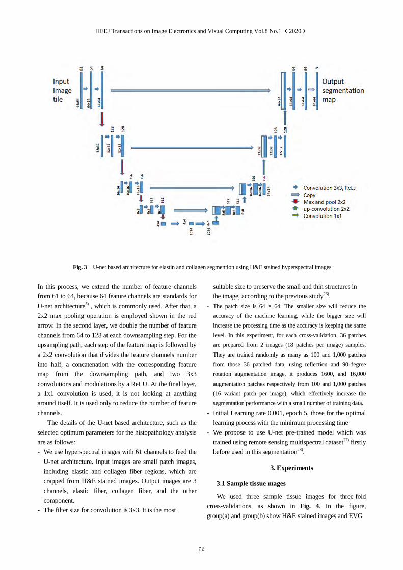
In this process, we extend the number of feature channels

from 61 to 64, because 64 feature channels are standards for

U-net architecture5) , which is commonly used. After that, a

2x2 max pooling operation is employed shown in the red

arrow. In the second layer, we double the number of feature

channels from 64 to 128 at each downsampling step. For the

upsampling path, each step of the feature map is followed by

a 2x2 convolution that divides the feature channels number

into half, a concatenation with the corresponding feature

map from the downsampling path, and two 3x3

convolutions and modulations by a ReLU. At the final layer,

a 1x1 convolution is used, it is not looking at anything

around itself. It is used only to reduce the number of feature

channels.

The details of the U-net based architecture, such as the

selected optimum parameters for the histopathology analysis

are as follows:

- We use hyperspectral images with 61 channels to feed the

U-net architecture. Input images are small patch images,

including elastic and collagen fiber regions, which are

crapped from H&E stained images. Output images are 3

channels, elastic fiber, collagen fiber, and the other

component.

- The filter size for convolution is 3x3. It is the most

suitable size to preserve the small and thin structures in

the image, according to the previous study26).

- The patch size is 64 × 64. The smaller size will reduce the

accuracy of the machine learning, while the bigger size will

increase the processing time as the accuracy is keeping the same

level. In this experiment, for each cross-validation, 36 patches

are prepared from 2 images (18 patches per image) samples.

They are trained randomly as many as 100 and 1,000 patches

from those 36 patched data, using reflection and 90-degree

rotation augmentation image, it produces 1600, and 16,000

augmentation patches respectively from 100 and 1,000 patches

(16 variant patch per image), which effectively increase the

segmentation performance with a small number of training data.

- Initial Learning rate 0.001, epoch 5, those for the optimal

learning process with the minimum processing time

- We propose to use U-net pre-trained model which was

trained using remote sensing multispectral dataset27) firstly

before used in this segmentation28).

3. Experiments

3.1 Sample tissue mages

We used three sample tissue images for three-fold

cross-validations, as shown in Fig. 4. In the figure,

group(a) and group(b) show H&E stained images and EVG

Fig. 3 U-net based architecture for elastin and collagen segmention using H&E stained hyperspectral images


20

Fig. 5 64 × 64 patch (a) Hyperspectral image (4 band images are extracted from 61 band ones), (b) corresponding RGB image, (c) Label

Fig. 4 H&E stained images of sample 1,2,3: (a-1), (a-2), (a-3); and EVG stained images of sample 1,2,3:(b-1), (b-2), (b-3)

(a) (b) (c)

Fig. 6 Cross-validation 1 segmentation result (a) RGB image, (b) Hyperspectral image, (c) Groundtruth image

(a-1) (a-2) (a-3)

(b-1) (b-2) (b-3)


21

stained images, respectively. We used three images for

cross-validations as follows,

- Cross-validation 1: we extract the fiber area from samples

2 and 3, then be tested in sample 1.





Training process use parameter mentioned in section 2.2. Figure 5 (a)-(c) show examples of 64×64 patch of a hyperspectral image, a corresponding RGB image, and its

label, respectively. The label in (c) consists of three classes, i.e., elastic, collagen, and other components obtained by applying Abe’s method to EVG stained images5) and corrected by the pathologist.

3.2 Segmentation result

We obtained segmentation results of elastic and collagen

fiber regions using three cross-validations. We compared the

segmentation result of the hyperspectral images to the

conventional RGB images.

Figure 6, 7 and 8 show the results of segmentation using

cross-validation 1,2 and 3, respectively. In each figure, (a)

and (b) denote segmentation result images obtained from

hyperspectral and RGB images, respectively, and (c)

(a) (b) (c)

Fig. 7 Cross-validation 2 segmentation result: (a) RGB image, (b) Hyperspectral image, (c) Groundtruth image

(a) (b) (c)

Fig. 8 Cross-validation 3 segmentation result: (a) RGB image, (b) Hyperspectral image, (c) Groundtruth image

Fig. 9 Dice coefficients of hyperspectral and RGB images using spectral-spatial features (U-net)


22

denotes a ground truth image obtained from EVG stained

image5). The blue and red color represents elastic and

collagen fiber, respectively. These results show that RGB

results have more misclassification than hyperspectral

images compared to ground truth images. We also evaluate the segmentation results quantitatively

by calculating the classification accuracy using the

following equation29),

Dice Coefficient = � �� (2)

True Positive (TP) is the number of pixels where elastic

fibers are decided as elastic fiber correctly, False Positive

(FP) is the number of pixels where collagen fibers are

decided as elastic fibers incorrectly, and False Negative (FN)

is the number of pixels where elastic fibers are decided as

collagen fibers incorrectly in the segmented images.

red bars show the dice coefficients of RGB images for 100

patches, yellow bars show the dice coefficients of

hyperspectral images for 1,000 patches, and purple bars

show the dice coefficients of RGB images for 1,000 patches.

From these data, we can see that the proposed U-net using

hyperspectral images performs better than RGB both using

100 and 1,000 patch numbers.

4. Discussion

In section 3, it has been observed that the proposed

method has a significantly better performance than RGB

images . Also, we compared the proposed method based on

spectral-spatial features to the previous sudy based on spectral

features 12).

Figure 10 shows the dice coefficients of hyperspectral

and RGB images using spectral features with LDA. Blue

bars show the dice coefficient of the hyperspectral images,

and red bars show the dice coefficient of RGB images.

Figure 11 shows the dice coefficients of hyperspectral

images using spectral-spatial features with U-net and

hyperspectral images using spectral features with LDA.

Blue and red bars show the dice coefficients of U-net using

100 and 1000 patches, respectively, and yellow bars show

the dice coefficients of LDA.

These results indicate that the segmentation of elastic

and collagen fibers using hyperspectral images perform

better results than RGB images in case of both using the

spectral feature only and the combination of spectral-spatial

features. In a comparison of spectral-spatial features with

U-net and spectral features with LDA, the former ones can

classify the elastic and collagen fiber regions with better

accuracy. These results were also subjectively evaluated by

pathologists from Saitama Medical University, and they

gave comments that the segmented images were almost

equivalent to the diagnostic outcome by pathologists, and

the results of spectral-spatial features with U-net were

especially well-classified.

Fig. 10 Dice coefficients of hyperspectral and RGB

images using spectral features (LDA)

Fig. 11 Dice coefficients of hyperspectral images usingspectral-spatial features (U-net) and spectral features (LDA)

Table 1 Average learning time

Number of patch images

Average learning

time

100 200 [sec]

1,000 1,850 [sec]


23

Table 1 shows the average learning time for validations

in this experiment. The software for calculation is Matlab

2019a, and the processor is NVIDIA™ Titan X. This result

shows that 1000 patch images take more than 9 times of 100

patch images, whereas data size of training is 10 times.

This experiment is our first trial for the segmentation of

elastic and collagen fibers. Thus, the developed U-net might

have much room to improve because we have tried only a

few kinds of parameters such as the architecture of U-net,

type of input data, number of training data set, and so on. If

we will repeat more trial-and-errors, it is sure that the

accuracy will increase.

5. Conclusion

In H&E stained images, it is difficult to distinguish

collagen and elastic fibers because these are similar in color

and texture.This study observed the segmentation of elastic

and collagen fibers from the H&E stained images through

hyperspectral transmittance using U-net based

spectral-spatial analysis. Groundtruth of the segmentation is

obtained using EVG stained images, which are commonly

used for recognizing elastic and collagen fiber regions. Our

model is evaluated by three cross-validations. The

segmentation results show that the combination of spatial

and spectral features in H&E stained hyperspectral images

performed better segmentation than H&E stained

conventional RGB images both in visual appearance and

quantitative verification.

This method is not only for visualization but also for

pixel wise classification. We believe that this method may

help the diagnostic accuracy increase.

Acknowledgment

The authors appreciate to Indonesia Endowment Fund

for Education (LPDP) and Join research program between

Japan Society for the Promotion of Science (JSPS) and

Indonesian Institute of Sciences (LIPI), for providing

financial support.

References

1) M. Titford: “The Long History of Hematoxylin”, Biotechnic &

Histochemistry. Vol.80 , No.2, pp.73‒78 (2005).

2) J. Uitto, L. Ryhanen, P.A. Abraham, A.J. Perejda: “Elastin in

Diseases”, The Journal of Investigative Dermatology, Vol. 79, Issue

1, Supplement, pp.160‒168 (1982).

3) Y. Yasui, T. Abe, M. Kurosaki, M. Higuchi, Y. Komiyama, T.

Yoshida, T. Hayashi, K. Kuwabara, K. Takaura, N. Nakakuki, H.

Takada, N. Tamaki, S. Suzuki, H. Nakanishi, K. Tsuchiya, J. Itakura,

Y. Takahashi, A. Hashiguchi, M. Sakamoto, N. Izumi: “Elastin Fiber

Accumulation in Liver Correlates with the Development of

Hepatocellular Carcinoma”, PloS one, Vol.11, No.4, e0154558

(2016).

4) E.Lakiotaki, S. Sakellariou, K, Evangelou, G. Liapis, E. Patsouris, I.

Delladetsima, Vascular and Ductal Elastotic Change in Pancreatic

Cancer, Acta Pathologica, Microbiologica et Immunologica

Scandinavica, John Wiley and Son (2015).

5) T. Abe, A. Hashiguchi, K. Yamazaki, H. Ebinuma, H. Saito, H.

Kumada, N. Izumi, N. Masaki, M. Sakamoto: “Quantification of

Collagen and Elastic Fibers Using Wholeslide Images of Liver

Biopsy Specimens”, Pathology International Vol.63, Issue 6, pp

305‒310, QA, June (2013).

6) www.polyscience.com, accessed on 12 October (2019)

7) M. Ishikawa, C. Okamoto, K. Shinoda, H. Komagata, C. Iwamoto, K.

Ohuchida, M. Hashizume, A. Shimizu, N. Kobayashi: “Detection of

Pancreatic Tumor Cell Nclei via a Hyperspectral Analysis of

Pathological Slides Based on Stain Spectra”,Biomedical Optics

Express, Vol. 10, No. 9, pp.4568–4588 (2019).

8) D. L. Farkas, C. Du, G. W. Fisher, C. Lau, W. Niu, E. S. Wachman,

R. M. Levenson:“Non-invasive Image Acquisition and Advance

Processing in Optical Bioimaging”, Computerized Medical Imaging

and Graphics Vol. 22, No.2, pp.89–102 (1998).

9) B. C. Wilson, S. L. Jacques: “Optical Reflectance and

Transmittance of Tissues: Principles and Applications”, IEEE

Journal of Quantum Electronics; Vol.26, Issue 12, pp.2186–98

(1990).

10) G. Lu, J. V. Little, X. Wang, H. Zhang, M. R. Patel, C. C. Griffith,

M. W. El-Deiry, A. Y. Chen, B. Fei:“Detection of Head and Neck

Cancer in Surgical Specimens using Quantitative Hyperspectral

Imaging”, Clin Cancer Res.; 23(18): pp.5426–5436. September 15

(2017).

11) P. A. Bautista, T. Abe, M. Yamaguchi, Y. Yagi, N. Ohyama:

“Digital Staining for Multispectral Images of Pathological Tissue

Specimens Based on Combined Classification of Spectral

Transmittance”, Computerized Medical Imaging and Graphics

Vol.29, Issue 8, pp. 649–657 (2005).

12) L. Septiana, H. Suzuki, M. Ishikawa, T. Obi, N. Kobayashi, N.

Ohyama, T. Ichimura, A. Sasaki, E. Wihardjo, D. Andiani: “Elastic

and Collagen Fibers Discriminant Analysis using H&E Stained

Hyperspectral Images”, Journal of Optical Review, Vol. 26, Issue 4,

pp. 369–379. Springer (2019).

13) V. P. Eroschenko, S. H. Mariano: “DiFiore's Atlas of Histology with

Functional Correlations”, 12th ed. Philadelphia, PA: Wolter Kluwer

Health/Lippincott Williams and Wilkins (2013).

14) T. Ushiki, Collagen Fibers: “Reticular Fibers and Elastic Fibers. A

Comprehensive Understanding from a Morphological Viewpoint”,

Arch. Histol. Cytol., Vol. 65, No. 2 (2002).

15) T. L. Sellaro, R. Filkins, C. Hoffman, J. L. Fine, J. Ho, A. V.

Parwani, L. Pantanowitz, M. Montalto: “Relationship between

Magnification and Resolution in Digital Pathology Systems”, Journal

of Pathology Informatics, (22 Aug.) Wolters Kluwer-Medknw

(2013).


24

16) D. L. Omucheni, K. A. Kaduki, W. D. Bulimo, H. K. Angeyo:

“Application of Principal Component Analysis to

Multispectral-Multimodal Optical Image Analysis for Malaria

Diagnostics”, Malaria Journal, 13:485 (2014).

17) L. Septiana, H. Suzuki, M. Ishikawa, T. Obi, N. Kobayashi, N.

Ohyama: “Staining Adjustment of Dye Amount to Clarify the

Appearance f Fiber, Nuclei, and Cytoplasm in HE-stained

Pathological Kidney Tissue Image”, International Multidiciplinary

Conference and Productivity and Sustainability, Ukrida press (2017).

18) T. Abe, Y. Murakami, M. Yamaguchi, N. Ohyama, Y. Yagi : “Color

Correction of Pathological Images Based on Dye Amount

Quantification”, Optical Review 12: 293 (2005).

19) H. Yuan, Y. Y. Tang, Y. Lu, L. Yang, H. Luo: “Spectral-Spatial

Classification of Hyperspectral Image Based on Discriminant

Analysis”, IEEE Journal of Selected Topics in Applied Earth

Obsevations and Remote Senssing Vol. 7, Issue 6, pp.2035–2043,

June (2014).

20) M. Fauvel, J. A. Benediktsson, J. Chanussot, J. R. Sveinsson:

“Spectral and Spatial Classification of Hyperspectral Data Using

SVMs and Morphological Profiles”, IEEE Trans. on Geoscience and

Remote Sensing, Vol.46, No.11, November (2008).

21) O. Ronneberger, P. Fischer, T. Brox: “U-Net: Convolutional

Networks for Biomedical Image Segmentation”, Computing

Research Repository (CoRR), abs/1505.04597 (2015).

22) M. Stokes, M. Anderson, S. Chandrasekar, R. Motta: “A Standard

Default Color Space for the Internet sRGB”, Microsoft and

Hewlett-Packard Joint Report, November 5 (1996).

23) H. L. Shen, P. Q. Cai, S. J. Shao, J. H. Xin : “Reflectance

reconstruction for multispectral imaging by adaptive Wiener

estimation”, Optics Express, Vol 15, Issue.23, pp.15545-15554, Nov.

(2007).

24) Mathwork. (2018). “Computer Vision System Toolbox

Documentation” (r2018). Retrieved December 15, (2018).

25) Mathwork, (2019). “Semantic Segmentation of Multispectral Images

using Deep Learning”, Image Processing Toolbox document

R2019a.Retrieved March 28, (2019).

26) P. S. Chavez, B. Bauer: “An Automatic Optimum Kernel-Size

Selection Technique for Edge Enhancement”, Remote Sensing Of

Environment Vol.12, Issue 1, pp.23–38 (1982).

27) http://www.cis.rit.edu/~rmk6217/rit18_data.mat, Retrieved

December 28, (2018).

28) R. Kemker, C. Salvaggio, C. Kanan: “High-Resolution Multispectral

Dataset for Semantic Segmentation”, Computing Research

Repository (CoRR), abs/1703.01918. (2017).

29) A. A. Taha, A. Hanbury: “Metrics for Evaluating 3D Medical Image

Segmentation: Analysis, Selection, and Tool”, BMC Medical

Imaging 15:29, (2015).

(Received July 27, 2019)

(Revised December 24, 2019)

Lina SEPTIANA She received B.Eng degree from Electronic Eng. Dept., Satya Wacana Christian Univ., Indonesia. M. Sc degree from Electrical Eng. and Computer Science Dept., Chung Yuan Christian Univ., Taiwan. Currently, she is a doctoral student in Information and Communication Eng. Dept. Tokyo Institute of Technology, Japan, and Lecturer at Engineering and Computer Science Fac. Krida Wacana Christian Univ. Indonesia.

Hiroyuki SUZUKI He received B.E., M.E., and Ph.D. degree from Tokyo Inst. of Tech. in 1998, 2000, and 2006, respectively. He was a Reseacher from 2003 to 2016. He has been an Assistant Professor with Institute of Innovative Research, Tokyo Inst. of Tech since 2016. His research interests include optical information security, hologram, biometric authentication, and medical healthcare information system.

Masahiro ISHIKAWA (Member) He received a Ph.D degree from Niigata University, Japan in 2006. He is currently an Assistant Professor at the Saitama Medical University. His current research interests include image processing and computer aided diagnosis.

Takashi OBI He earned B.S. degree in Physics, M.S. and Ph.D. degree in Information Physics from Tokyo Inst. of Tech, Japan in 1990, 1992, and 1996 respectively. Currently, he is an Associate Professor of Laboratory for Future Institute of Innovative Research, Tokyo Inst. of Tech. His Research focuses on medical informatics, information system and security, etc. He is a member of IEICE, JAMIT, JSAP, JSNM, JSMP, and IEEE.

Naoki KOBAYASHI (Fellow) He earned B.Sc., M.E. degree from Tokyo Inst. of Tech, in 1979, 1981 respectively. Ph. D degree from Niigata Univ in 2000. He worked for NTT Lab. In 1981-2008. He has been at professor at School of Biomed. Eng, Fac. of Health and Medical Care, Saitama Medical Univ. since 2008. His research interests include medical image processing, image compression, and biosignal processing, He is a member of IECE, IIEEJ, JSMBE, and IEEE.


25

Nagaaki OHYAMA He earned Doc. Eng. degree in Information Physics from Tokyo Inst. of Tech. in 1982. His academic career on Tokyo Inst. of Tech has been started since 1982. Become professor in Tokyo Inst. of Tech since 1993. His current research project is related to Japan government's information policy (formulation of electronic preservation standards for medical images, onlin request for claims, introduction of public personal authentication service, etc.)

Takaya ICHIMURA He earned M.D., Ph.D. degress and is an assistant professor of the Saitama Medical University. He received the Ph.D. degree from Kumamoto University, Kumamoto, Japan, in 2005. His current research interests include nuclear atypia and the molecular nature of chromatin.

Atsushi SASAKI He earned M.D., Ph.D. degrees from Gunma Univ. School of Medicine in 1980, 1984, respectively. He received the Neuropathology Best Paper Award in 2001, Brain Tumor Pathology Best Paper Award in 2002. He is currently a professor at the Dept. of Pathology, Saitama Medical Univ. His research interests include brain tumor pathology and microglia. Dr. Sasaki is a member of the International Society of Neuropathology and American Association of Neuropathologists.

Erning WIHARDJO He earned B.Sc., M.Sc. in Physics from Padjajaran Univ. Indonesia in 1976. M. Eng in Opto-Electronics, Univ. of Indonesia in 1979. M. Eng., Doc. Eng. in Physical Information from Tokyo Inst. of Tech. in 1983 and 1986 respectively. He was a scientist at the Indonesia Inst. of Science and Polycore Optical. Ltd., Singapore in 1986-1995. He continued his career at Hoya Lens Ltd in 1995-2012, with the latest position as Director of Hoya Asia H.Q, Singapore. He was awarded professorship from the He Univ. of Ophthalmology and Visual Science, China in 2008. He is the president of Krida Wacana Christian. Univ. Indonesia 2016 - 2020.

Harry ARJADI He is a senior scientist at Indonesian Institute of Sciences, Research Center for Quality System and Testing Technology (P2SMTP-LIPI), Indonesia. He earned B.Sc., in Physical Eng. from Bandung Inst. of Tech. Indonesia in 1981, M. Sc. In Electronic Intrumentation Design, Ph. D. in Bio-Electromagnetic from Salford Univ. U.K. in 1988 and 1992 respectively.


26

IIEEJ Paper

Pressure Sensitivity Pattern Analysis Using Machine Learning Methods

Henry FERNANDEZ† , Koji MIKAMI† , Kunio KONDO†(Fellow)

†Tokyo University of Technology

<Summary> As a consequence of a lack of balance between the levels of difficulty of a game and the

players’ skills, the resulting experience for players might be frustrating (too difficult) or boring (too easy).

Players having a bad experience could impact game creators negatively, leading to irreparable damage. The

main motivation of this study was to find effective ways to reduce the gap between skills and difficulty,

to help developers create a more suitable experience for players. This paper shows the results of applying

Neural Networks and Support Vector Machines to data collected from the pressure exerted to a gamepad’s

button with the purpose of finding patterns that can help predict: difficulty, fun, frustration, boredom,

valence, arousal and dominance at a determined time. We obtained results with an accuracy of 83.64 %

when predicting boredom, around 70 % of accuracy classifying frustration, fun, difficulty and dominance.

Keywords: game design, game development, pressure sensitivity, gamepad, machine learning, feelings,

neural networks, support vector machines, behavioral pattern

1. Introduction

The ultimate goal of our research is to adapt the expe-

rience for players with different skills. We wanted to find

new ways to correct the imbalance that sometimes ap-

pears in games due to differences between challenges’ dif-

ficulty and the ability of players to overcome those chal-

lenges. A large gap between the players’ skills and levels

of difficulty for challenges that they encounter in a game,

might impact the overall experience in a negative way, in

consequence, making players quit1)–4). Enjoyment, fun,

engagement, have been topics of study for a wide range

of researchers in the academia5)–11), we would like to con-

tribute by exploring this topic using behavioral patterns

and how they relate to the player’s status and perceptions

while playing.

So far we have been working with Dynamic Difficulty

Adjustment, Procedural Content Generation and Brain

Computer Interface applied to 2D platform games and

the focus of those studies was to understand the possible

relationships between player experience and perception of

difficulty12),13). Our second approach involves behavioral

patterns, specifically, the relationship between the pres-

sure exerted on a gamepad’s button and players’ emo-

tions, including how players perceive the current status

of the game.

We divided the problem in three steps: (1) data collec-

tion, (2) classification method and (3) difficulty adapta-

tion. Step (1) has been already completed. Is constituted

of an analysis of the data obtained from experiments in

a 2D shooting game, demonstrating that there is a clear

relationship between the evaluated parameters and the

force exerted on the gamepad’s button14). This paper

summarizes the results of step (2), in which we used the

data collected from an experiment conducted with 20 dif-

ferent players and tested it with machine learning meth-

ods to understand the player’s experience in real time.

Using machine learning methods would help us to find

patterns that could be used by developers to adapt in-

game parameters according to what players are experi-

encing and improve the final result. Step (3) is part of

our future work.

Support vector machines and neural networks are

widely used to classify data and make predictions in real

time15)–17). For our specific problem, which involves be-

havioral patterns related data, emotions and player’s per-

ceptions, some researchers working on the same topic

have achieved good results using machine learning meth-

ods18)–20), which is the main reason why we decided to

use neural networks and support vector machines in our

research.

Experiments were designed to make players interact as

much as possible with the gamepad’s button to be able

to collect large amounts of data. Players played 6 levels



27

of a 2D space shooter, after finishing each level, question-

naires to measure their perception towards the game were

applied. The parameters measured in the questionnaires

are: difficulty, fun, frustration, boredom, valence, arousal

and dominance. In addition, in-game data was collected

for future analysis.

All the collected data was used with a set of different

machine learning algorithms, three different types of neu-

ral networks and support vector machines for each param-

eter measured in the questionnaires were designed. We

tested several times to obtain the best possible results

and input values for each method. One of the clearest

results of our analysis was that support vector machines

can classify pressure sensitivity with better accuracy than

neural networks, for neural networks with an average ac-

curacy result of 68.55 % and for support vector machines,

an average result of 70.69 %.

In this paper, our results also demonstrated that the

easiest parameters to classify are: boredom (83.64 %),

difficulty (72.17 %), dominance (71.13 %), frustration

(70.27 %) and fun (70.14 %), and the rest of the results’

accuracy was above 60 %. Although the way we ana-

lyzed the presented results and this previous research19)

are not exactly the same, we were able to achieve more

than 60 % of accuracy for all parameters, while Chanel et

al. AI could classify boredom, engagement and anxiety

with 53.33 % of accuracy.

2. Related Work

In a previous research, Sykes et al. used a PlaySta-

tion 2 controller to measure pressure sensitivity and its

correlation with arousal in experiments conducted using

a clone of ‘Space Invaders’21). This was one of the first

known studies that proved that pressure sensitivity was

directly related to the player’s emotions. We decided to

use some of the elements from this research, our exper-

iment was conducted with a 2D shooter and a PlaySta-

tion 3 gamepad (with the same pressure sensitivity capa-

bility).

As a relevant result from the research of van den

Hoogen et al., when players felt more aroused and domi-

nant while playing a racing game they put more pressure

on the controller, demonstrating the relationship between

pressure and emotions22). Unlike our research, which is

focused on the force applied to the button of a gamepad,

these researchers measured the pressure on the controller

itself, a different approach to measuring physical behav-

iors. The same group of researchers demonstrated that

player experience can be quantified through the behav-

ior of players, measuring the force applied to a keyboard,

they obtained levels of arousal23).

In previous studies, researchers designed a method to

inform developers when a series of actions performed in-

side a game represent a frustrating event for players24).

The focus of this research was to detect emotions such as

boredom, frustration or the state of flow. Their method

was specific for a particular game but we think that the

approach could be used for a more general purpose.

For a different group of participants in a field not re-

lated to games, a group of programmers were analyzed by

using biometric sensors and self-reports to classify their

emotions25). They obtained an accuracy of 71.36 % and

progress in 67.70 %, their research involved flow theory,

boredom, basically the same parameters that we used in

our study.

We designed the questionnaires for the experiments

using Self-Assessment Manikin (SAM), which was suc-

cessfully applied for studying emotions in people while

playing sounds in Portuguese26), this scale was also suc-

cessfully used to predict playing time and preferences in

games27). In our research, we measured valence, arousal

and dominance of players after playing each game session.

There are several studies that involve the recognition of

emotions and in-game player related parameters. Creat-

ing a recognition system using Support Vector Machines,

researchers classified affective states from players and col-

lecting speech signal data and an eye tracker20). Results

showed high accuracy by applying these methods and

they are being considered for improving the player in-

teraction.

In order to predict valence, arousal and dominance,

researchers focused on using random forests to prevent

undesired emotions when playing videogames18). As a

result from this study, Frommel et al.18) proposed an ar-

chitecture to react to player’s emotions using procedural

content generation and emotion detection.

Physiological and self-reported data, in combination

with support vector machines were used to predict emo-

tions and to keep players engaged while playing a game

by adapting its difficulty automatically according to the

predicted outputs19). Although our approach is similar

to this research, there are significant differences:

• Instead of using physiological data, we focused on

pressure exerted on the button of a gamepad which

opens up the possibility for adding real time changes


28

based on behavioral patterns.

• Our approach did not only involve Support Vector

Machines, we tested Neural Networks, which proved

to be successful too.

• We predicted fun, frustration, boredom, valence,

arousal and dominance using pressure sensitivity as

input. In the previous research, these parameters

were used to adapt the game difficulty.

• The accuracy of our results is higher.

Using physiological signals, it was shown that game ex-

perience can be accurately predicted28). A machine learn-

ing method was implemented to classify difficulty, im-

mersion and amusement from players while playing FIFA

2016. This study involved physiological signals, facial

recognition, game screen recording and in-game data.

Using flow theory and cognitive load theory to trigger

engagement on players, researchers designed a new adap-

tive method that yielded successful results by compar-

ing their proposal with traditional gameplay and choice-

based gameplay29),30).

Considering that previous research has demonstrated

that players’ behavior is not only directly related to what

they experience but also can be classified and estimated,

we decided to combine similar elements from previous

studies and include them in our approach. We attempt

to measure and understand players’ emotions and game

related parameters using machine learning methods.

3. Game Details

The game we designed for data collection was a 2D

space shooting game with basic features. Players control

a spaceship that could move throughout the screen with-

out rotation, having the possibility to shoot straight at

any time and with no constraints of ammo or time limi-

tations. As main goal for the game, players are required

to clear several waves of enemies that approach from the

Fig. 1 A screenshot of a gameplay scene (Player: orangespaceship; Enemies: have to be destroyed by theplayer)

upper part of the screen and shot in different ways. Three

lives and three bars of health are included, with the possi-

bility to recover them using items. A sample of gameplay

can be seen in Fig. 1. For more information about the

details of design and implementation, please refer to14).

There are several reasons for choosing this type of game

for our research:

• We wanted a game in which players are required to

press the controller’s button repeatedly in order to

collect enough data for the analysis

• This type of shooting game is well-known by a wide

audience

• The same type of game was used in a previous re-

search, showing successful results21), giving us the

possibility to have a comparison referent

The level design was established using several parame-

ters to decide what enemies and how many of them would

appear in each wave. Difficulty is changed by modifying

the enemies’ skills and behavior.

Enemies are able to shoot from 1 to 4 bullets at the

same time. In addition, enemies had different movement

patterns and health, creating a more challenging and var-

ied gameplay. Specific implementation details can be seen

in our previous work14).

4. Experiment

Experiments are designed to collect data from the pres-

sure exerted on the button’s controller. These are the

parameters that we measured in the experiment: dif-

ficulty, fun, boredom, frustration, valence, arousal and

dominance. Figure 2 shows a diagram of the experi-

ment. Threshold method was used to decide the baseline

for the difficulty and 6 levels were played after that.

4.1 Structure

As illustrated by Fig. 2, the experiment is structured

in two parts:

1. Threshold method: which served as a baseline to

know the players’ skills, letting them play until they

died

Fig. 2 Experiments layout


29

Fig. 3 Self-Assessment Manikin test

2. Randomly choose and play: which included easy

(easier than the medium level), medium (last level

played in the threshold method) and difficult (harder

than the medium level) levels that were presented to

players in a random order.

4.2 Experience questionnaire

Players were asked to fill out a questionnaire about

their experience after playing one level. Questions were

divided in two parts: (1) game-related questions and (2)

SAM questions.

For part 1, players were questioned about: difficulty of

the level, how much fun they had, how frustrated they

felt and how bored they felt. All questions were designed

using a Likert scale of 5 points.

The second part of the questionnaire was focused on

measuring the player’s feelings. For this section, we used

a Self-Assessment Manikin (SAM) test, in which play-

ers were required to quantify their emotions using a pre-

defined scale (see Fig. 3) towards the game from the

experiment in three different categories: valence, arousal

and dominance. Looking at the numbers from 1 to 9

and using the images as a reference, participants had to

choose the value that best represented their feelings in

each category.

4.3 Pressure sensitivity

Pressure exerted on the button of a PS3 controller

gamepad was saved and used to create the model. Pres-

sure is a value between 0 and 1 that indicates how hard

the player presses a button in the controller. 1 means

fully pressed and 0 means the button is not pressed.

Figure 4 shows the results of a sample taken from one

session. The horizontal axis shows the time in seconds

and vertical axis shows the pressure values recorded when

pressing the shooting button.

Table 1 Number of samples per classCla Dif Fun Fru Bor Val Aro Dom

1 38092 49921 34067 29263 53513 65464 64987

0 85394 73565 89419 94223 69973 58022 58499

Fig. 4 Sample taken from one player after playing onelevel of the game

5. Machine Learning: Data Classification

One neural network and one support vector machine

were created for each parameter (fun, frustration, etc.),

they were trained and tested separately and indepen-

dently from each other with different parameters and con-

figuration.

5.1 General idea

Data was pre-processed before being used with the

models and the output for each system was converted

to the space of 0s and 1s, the general approach is repre-

sented in figure 5.

5.1.1 Input data

Collected data from all users (20 people) constituted

a total number of 123486 samples. We used the method

Leave One Out (LOO), which is a special case of cross-

validation where one participant’s data is used to test

and the rest of the data to train the model; this process

is repeated until all participants’ data is used31).

This validation model ensures that the systems can

classify input data from a new user in a reliable way.

We did not divide the data or the players’ results by pro-

ficiency when designing and validating our models. The

input length of our models was 5, we determined this

value by testing with different input sizes and choosing

the one with the best result.

Table 1 shows the details of each class for each param-

eter.

5.1.2 Pre-processing and labeling

All data was separated and labeled according to the an-

swers given by players while doing the experiment. After

completing one full session in the game, all the collected

data for that specific session was classified using the given


30

Fig. 5 General approach: Use input data in a machinelearning method to predict parameters

answers, as an example, if the player rates one session as

’very difficult’, all the input will be labeled as ’very diffi-

cult’ for that session.

Since the pace in one level can change from easier to

harder while progressing, labelling all the input values

in one specific category could lead to loss of granularity

about what the player is really feeling in each part of the

game, this is why we decided to pre-process the data and

calculate the average of each input by the time the input

was stored. Using the average data of each input value,

allowed us to work with the tendency of that session in-

stead of values in a specific time.

5.1.3 Output data codification

As we mentioned in section 4.2, questions for the first

four parameters were designed using a Likert scale of 5

points; the second part of the questionnaire was designed

using the SAM method which consisted of 9 different an-

swers for each parameter.

In order to use the collected data for the mentioned

machine learning methods, we grouped the output vec-

tor according to three different categories: low, medium

and high. Parameters that were originally codified with

5 outputs were transformed to a binary output and pa-

rameters that were originally codified as 9 outputs, were

transformed to a binary output as well. That is to say

that we created one specific machine for each parame-

ter (7 parameters); for each group of that parameter (3

groups); for each method (2 methods); for a total of 42

different machines.

5.2 Implementation

All the evaluation was conducted using the free soft-

ware machine learning library Scikit-learn. We conducted

a series of preliminary simulations for each system and we

chose the parameters with the best results, which are the

results presented in this paper.

• Neural Network’s Parameters:

– Rate: Constant

– Activation function: Relu

– Number of hidden nodes: 100

– Max. iterations: 1000

– Solver: lbfgs

• Support Vector Machine’s Parameters:

– Kernel: Radial Basis Function

– Degree: 3

– C-Parameter: 1

– Gamma: 1n (being n the number of features)

5.3 Accuracy calculation

Accuracy for each model was calculated by obtaining

the mean value of all accuracy results for each iteration

of the LOO cross validation. Equation (1) shows the for-

mula to calculate the overall accuracy for each model.

M(X,Y ) =1

n

n−1∑

i=0

A(Xi, Yi) (1)

where:

• X represents a set with all the Leave One Out train-

ing data; Y is a set with all the expected outcomes

for X.

• A(Xi, Yi) is the accuracy calculated for the specific

set i. This function is defined in equation (2).

A(x, y) =1

n

n−1∑

i=0

f(x = y) (2)

where:

• x represents the test data; y the expected outcome

for x.

• f(x = y) indicates whether x is equal to y or not.

6. Results and Discussion

Examined data was collected from 20 participants with

different game skills and characteristics. 75% of the play-

ers were male and their age was ranged between 12 and 44

years old. Players with low, medium and high experience

were tested.

6.1 Survey of the results

All the average results can be seen in Figure 6, show-

ing all the evaluated parameters from the questionnaires

in the horizontal axis, vertical axis shows the calculated

accuracy.

The best result was achieved for boredom, with 83.64 %

of accuracy with SVM; difficulty, fun, frustration and

dominance, were predicted with around 70 % of accuracy.

In general, support vector machines performed better

than neural networks for all parameters except frustra-

tion. The average accuracy (all parameters) for neural


31

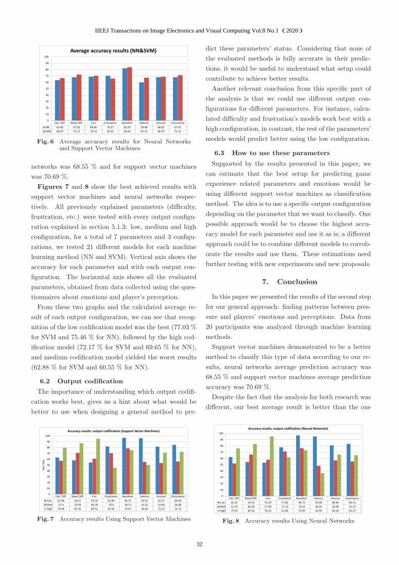
Fig. 6 Average accuracy results for Neural Networksand Support Vector Machines

networks was 68.55 % and for support vector machines

was 70.69 %.

Figures 7 and 8 show the best achieved results with

support vector machines and neural networks respec-

tively. All previously explained parameters (difficulty,

frustration, etc.) were tested with every output configu-

ration explained in section 5.1.3: low, medium and high

configuration, for a total of 7 parameters and 3 configu-

rations, we tested 21 different models for each machine

learning method (NN and SVM). Vertical axis shows the

accuracy for each parameter and with each output con-

figuration. The horizontal axis shows all the evaluated

parameters, obtained from data collected using the ques-

tionnaires about emotions and player’s perception.

From these two graphs and the calculated average re-

sult of each output configuration, we can see that recog-

nition of the low codification model was the best (77.03 %

for SVM and 75.46 % for NN), followed by the high cod-

ification model (72.17 % for SVM and 69.65 % for NN),

and medium codification model yielded the worst results

(62.88 % for SVM and 60.55 % for NN).

6.2 Output codification

The importance of understanding which output codifi-

cation works best, gives us a hint about what would be

better to use when designing a general method to pre-

Fig. 7 Accuracy results Using Support Vector Machines

dict these parameters’ status. Considering that none of

the evaluated methods is fully accurate in their predic-

tions, it would be useful to understand what setup could

contribute to achieve better results.

Another relevant conclusion from this specific part of

the analysis is that we could use different output con-

figurations for different parameters. For instance, calcu-

lated difficulty and frustration’s models work best with a

high configuration, in contrast, the rest of the parameters’

models would predict better using the low configuration.

6.3 How to use these parameters

Supported by the results presented in this paper, we

can estimate that the best setup for predicting game

experience related parameters and emotions would be

using different support vector machines as classification

method. The idea is to use a specific output configuration

depending on the parameter that we want to classify. One

possible approach would be to choose the highest accu-

racy model for each parameter and use it as is; a different

approach could be to combine different models to corrob-

orate the results and use them. These estimations need

further testing with new experiments and new proposals.

7. Conclusion

In this paper we presented the results of the second step

for our general approach: finding patterns between pres-

sure and players’ emotions and perceptions. Data from

20 participants was analyzed through machine learning

methods.

Support vector machines demonstrated to be a better

method to classify this type of data according to our re-

sults, neural networks average prediction accuracy was

68.55 % and support vector machines average prediction

accuracy was 70.69 %.

Despite the fact that the analysis for both research was

different, our best average result is better than the one

Fig. 8 Accuracy results Using Neural Networks


32

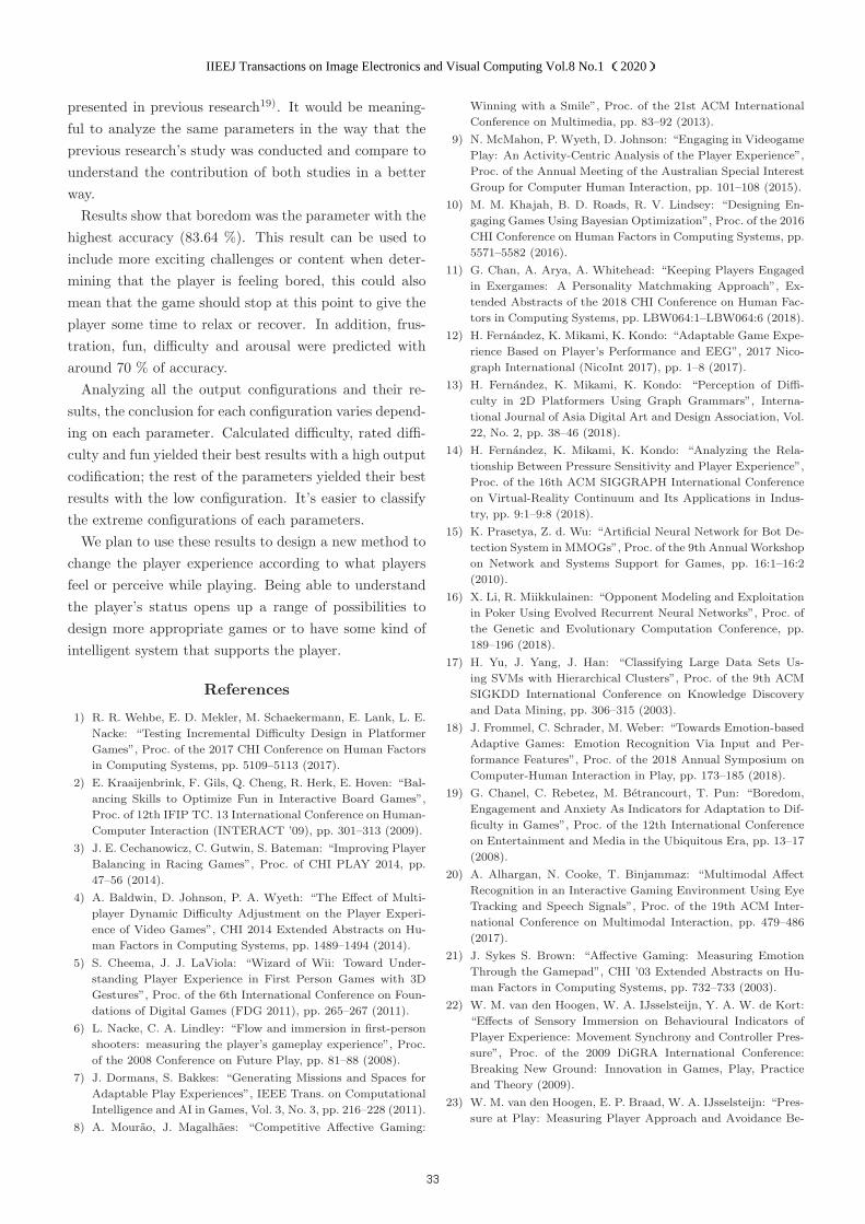
presented in previous research19). It would be meaning-

ful to analyze the same parameters in the way that the

previous research’s study was conducted and compare to

understand the contribution of both studies in a better

way.

Results show that boredom was the parameter with the

highest accuracy (83.64 %). This result can be used to

include more exciting challenges or content when deter-

mining that the player is feeling bored, this could also

mean that the game should stop at this point to give the

player some time to relax or recover. In addition, frus-

tration, fun, difficulty and arousal were predicted with

around 70 % of accuracy.

Analyzing all the output configurations and their re-

sults, the conclusion for each configuration varies depend-

ing on each parameter. Calculated difficulty, rated diffi-

culty and fun yielded their best results with a high output

codification; the rest of the parameters yielded their best

results with the low configuration. It’s easier to classify

the extreme configurations of each parameters.

We plan to use these results to design a new method to

change the player experience according to what players

feel or perceive while playing. Being able to understand

the player’s status opens up a range of possibilities to

design more appropriate games or to have some kind of

intelligent system that supports the player.

References

1) R. R. Wehbe, E. D. Mekler, M. Schaekermann, E. Lank, L. E.

Nacke: “Testing Incremental Difficulty Design in Platformer

Games”, Proc. of the 2017 CHI Conference on Human Factors

in Computing Systems, pp. 5109–5113 (2017).

2) E. Kraaijenbrink, F. Gils, Q. Cheng, R. Herk, E. Hoven: “Bal-

ancing Skills to Optimize Fun in Interactive Board Games”,

Proc. of 12th IFIP TC. 13 International Conference on Human-

Computer Interaction (INTERACT ’09), pp. 301–313 (2009).

3) J. E. Cechanowicz, C. Gutwin, S. Bateman: “Improving Player

Balancing in Racing Games”, Proc. of CHI PLAY 2014, pp.

47–56 (2014).

4) A. Baldwin, D. Johnson, P. A. Wyeth: “The Effect of Multi-

player Dynamic Difficulty Adjustment on the Player Experi-

ence of Video Games”, CHI 2014 Extended Abstracts on Hu-

man Factors in Computing Systems, pp. 1489–1494 (2014).

5) S. Cheema, J. J. LaViola: “Wizard of Wii: Toward Under-

standing Player Experience in First Person Games with 3D

Gestures”, Proc. of the 6th International Conference on Foun-

dations of Digital Games (FDG 2011), pp. 265–267 (2011).

6) L. Nacke, C. A. Lindley: “Flow and immersion in first-person

shooters: measuring the player’s gameplay experience”, Proc.

of the 2008 Conference on Future Play, pp. 81–88 (2008).

7) J. Dormans, S. Bakkes: “Generating Missions and Spaces for

Adaptable Play Experiences”, IEEE Trans. on Computational

Intelligence and AI in Games, Vol. 3, No. 3, pp. 216–228 (2011).

8) A. Mourao, J. Magalhaes: “Competitive Affective Gaming:

Winning with a Smile”, Proc. of the 21st ACM International

Conference on Multimedia, pp. 83–92 (2013).

9) N. McMahon, P. Wyeth, D. Johnson: “Engaging in Videogame

Play: An Activity-Centric Analysis of the Player Experience”,

Proc. of the Annual Meeting of the Australian Special Interest

Group for Computer Human Interaction, pp. 101–108 (2015).

10) M. M. Khajah, B. D. Roads, R. V. Lindsey: “Designing En-

gaging Games Using Bayesian Optimization”, Proc. of the 2016

CHI Conference on Human Factors in Computing Systems, pp.

5571–5582 (2016).

11) G. Chan, A. Arya, A. Whitehead: “Keeping Players Engaged

in Exergames: A Personality Matchmaking Approach”, Ex-

tended Abstracts of the 2018 CHI Conference on Human Fac-

tors in Computing Systems, pp. LBW064:1–LBW064:6 (2018).

12) H. Fernandez, K. Mikami, K. Kondo: “Adaptable Game Expe-

rience Based on Player’s Performance and EEG”, 2017 Nico-

graph International (NicoInt 2017), pp. 1–8 (2017).

13) H. Fernandez, K. Mikami, K. Kondo: “Perception of Diffi-

culty in 2D Platformers Using Graph Grammars”, Interna-

tional Journal of Asia Digital Art and Design Association, Vol.

22, No. 2, pp. 38–46 (2018).

14) H. Fernandez, K. Mikami, K. Kondo: “Analyzing the Rela-

tionship Between Pressure Sensitivity and Player Experience”,

Proc. of the 16th ACM SIGGRAPH International Conference

on Virtual-Reality Continuum and Its Applications in Indus-

try, pp. 9:1–9:8 (2018).

15) K. Prasetya, Z. d. Wu: “Artificial Neural Network for Bot De-

tection System in MMOGs”, Proc. of the 9th Annual Workshop

on Network and Systems Support for Games, pp. 16:1–16:2

(2010).

16) X. Li, R. Miikkulainen: “Opponent Modeling and Exploitation

in Poker Using Evolved Recurrent Neural Networks”, Proc. of

the Genetic and Evolutionary Computation Conference, pp.

189–196 (2018).

17) H. Yu, J. Yang, J. Han: “Classifying Large Data Sets Us-

ing SVMs with Hierarchical Clusters”, Proc. of the 9th ACM

SIGKDD International Conference on Knowledge Discovery

and Data Mining, pp. 306–315 (2003).

18) J. Frommel, C. Schrader, M. Weber: “Towards Emotion-based

Adaptive Games: Emotion Recognition Via Input and Per-

formance Features”, Proc. of the 2018 Annual Symposium on

Computer-Human Interaction in Play, pp. 173–185 (2018).

19) G. Chanel, C. Rebetez, M. Betrancourt, T. Pun: “Boredom,

Engagement and Anxiety As Indicators for Adaptation to Dif-

ficulty in Games”, Proc. of the 12th International Conference

on Entertainment and Media in the Ubiquitous Era, pp. 13–17

(2008).

20) A. Alhargan, N. Cooke, T. Binjammaz: “Multimodal Affect

Recognition in an Interactive Gaming Environment Using Eye

Tracking and Speech Signals”, Proc. of the 19th ACM Inter-

national Conference on Multimodal Interaction, pp. 479–486

(2017).

21) J. Sykes S. Brown: “Affective Gaming: Measuring Emotion

Through the Gamepad”, CHI ’03 Extended Abstracts on Hu-

man Factors in Computing Systems, pp. 732–733 (2003).

22) W. M. van den Hoogen, W. A. IJsselsteijn, Y. A. W. de Kort:

“Effects of Sensory Immersion on Behavioural Indicators of

Player Experience: Movement Synchrony and Controller Pres-

sure”, Proc. of the 2009 DiGRA International Conference:

Breaking New Ground: Innovation in Games, Play, Practice

and Theory (2009).

23) W. M. van den Hoogen, E. P. Braad, W. A. IJsselsteijn: “Pres-

sure at Play: Measuring Player Approach and Avoidance Be-


33

haviour through the Keyboard”, Proc. of the 2014 DiGRA In-

ternational Conference (2014).

24) A. Canossa, A. Drachen, J. Rau, M. Sørensen: “Arrrgghh!!!

-Blending Quantitative and Qualitative Methods to Detect

Player Frustration”, Proc. of the 6th International Conference

on the Foundations of Digital Games (2011).

25) Muller, T. Fritz: “Stuck and Frustrated or in Flow and Happy:

Sensing Developers’ Emotions and Progress”, Proc. of the 37th

International Conference on Software Engineering, Vol. 1, pp.

688–699 (2015).

26) A. P. Soares, A. P. Pinheiro, A. T. P. Costa, C. S. Frade, M.

Comesana, R. Pureza: “Affective auditory stimuli: adaptation

of the International Affective Digitized Sounds (IADS-2) for

European Portuguese”, Behavior research methods, Vol. 45,

No, 4, pp. 1168–1181 (2013).

27) K. Poels, W. M. van den Hoogen, Y. A. W. de Kort, W. A.

IJsselsteijn: “Pleasure to Play, Arousal to Stay : the Effect

of Player Emotions on Digital Game Preferences and Play-

ing Time”, Cyberpsychology, Behavior, and Social Networking,

Vol. 15, No, 1, pp. 1–6 (2012).

28) W. Yang, M. Rifqi, C. Marsala, A. Pinna: “Towards Better

Understanding of Player’s Game Experience”, Proc. of the 2018

ACM on International Conference on Multimedia Retrieval,

pp. 442–449 (2018).

29) D. Sharek E. Wiebe: “Measuring Video Game Engagement

Through the Cognitive and Affective Dimensions”, Simulation

& Gaming, Vol. 45, pp. 565–592 (2014).

30) D. Sharek E. Wiebe: “Investigating Real-time Predictors

of Engagement: Implications for Adaptive Videogames and

Online Training”, International Journal of Gaming and

Computer-Mediated Simulations, Vol. 7, No, 1, pp. 20–37

(2015).

31) C. Sammut, G. I. Webb, Eds.: Encyclopedia of Machine Learn-

ing, pp. 600–601, Springer US (2010).

Henry FERNANDEZHe obtained his PhD in Media Science at

the Tokyo University of Technology, his Mas-

ter’s degree in Engineering from the same

university and studied Computer Engineering

at the Simon Bolıvar University in Caracas,

Venezuela. His research interests are game

design, game production, programming and

2D art. He has been working as an indepen-

dent game developer at Fiery Squirrel since

2014.

Koji MIKAMIHe worked at Nissho Iwai Corporation and

MK Company as a producer. In 1998, he es-

tablished ”Creative Lab.” at the Katayanagi

Advanced Research Institute of Tokyo Uni-

versity of Technology (TUT), where research

on Animation, Game and CG production

technology are conducted. Currently, he is

a professor at the School of Media Science,

TUT. He received his Ph.D. degree at KEIO

University in 2018. Now his research interests

lie in game design and production technology

for game and animation.

Kunio KONDO (Fellow)

He is a professor at the School of Media Sci-

ence, Tokyo University of Technology. He re-

ceived his Ph.D degree from the University

of Tokyo in 1988. He was associate professor

of Department of Information and Computer

Sciences, Saitama University, and Technical

staff of Nagoya University. He is the president

of Asia Digital Art and Design Association.

He was former President of The Institute of

Image Electronics engineers of Japan, former

President of The Society for Art and Sci-

ence, and Chair of SIG on Computer Graphics

and CAD of Information Processing Society

of Japan.


34

Image Completion of 360-Degree Images by cGAN with Residual Multi-Scale Dilated

Convolution

Naofumi AKIMOTO, Yoshimitsu AOKI (Member)

Keio University

<Summary> In this paper, we are tackling the problem of the entire 360-degree image generation process by viewing one

specific aspect of it. We believe that there are two key points for achieving this 360-degree image completion: firstly,

understanding the scene context; for instance, if a road is in front, the road continues on the back side; and secondly, the

treatment of the area-wise information bias; for instance, the upper and lower areas are sparse due to the distortion of

equirectangular projection, and the center is dense since it is less affected by it. Although the context of the whole image can be

understood through using dilated convolutions in a series, such as recent conditional Generative Adversarial Networks

(cGAN)-based inpainting methods, these methods cannot simultaneously deal with detailed information. Therefore, we propose

a novel generator network with multi-scale dilated convolutions for the area-wise information bias on one 360-degree image

and a self-attention block for improving the texture quality. Several experiments show that the proposed generator can better

capture the properties of a 360-degree image and that it has the effective architecture for 360-degree image completion.

Keywords: generative adversarial networks, image completion, equirectanglur projection

1. Introduction

Equireqtanglar projection is one of the methods used for

representing a 360-degree space as an omnidirectional

image. Accompanied by the popularization of head-mounted

displays for virtual reality (VR) and a handy 360-degree

camera, there are increasing opportunities for 360-degree

images like these to be used. However, there is plenty of

difficulty and financial cost in designing a realistic

360-degree space with computer graphics. Therefore, as our

method for easily designing a 360-degree image space, we

favor the following approach: We can convert a picture with

a narrow angle of view taken by a smartphone to one

particular area of a 360-degree image by using internal

camera parameters. Then, we can produce a whole

360-degree space by completing the remaining area with

this one particular area as a necessary condition. The merit

of this approach is that we can selectively use many

normal camera images to determine the atmosphere of a

newly generated space, since the image being generated is

consistent with the conditional image. One example of the

more concrete applications is that a distant view of a new

VR space is easily attained. Additionally, since the

completion is performed, it is possible use the same method

to remove an object from the image of a 360-degree camera

where an unnecessary object is easily reflected.

This paper tackles the problem of the whole 360-degree

image being generated with one part as a condition, within

the above whole approach to space generation. The goal of

this problem setting is to reflect the specific properties of a

360-degree image in image generation. This involves two

specific points: understanding the context of the scene and

reflecting the differences in the amount of information in

360-degree images.

Figure 1 shows the 360-degree images and their

spherical visualization using an image sample. If there is a

road in front like in Fig. 1 (a), it is better to estimate that the

road continues on the back side. In the patch-based method2),

there is no path behind the image, because there is no

understanding of the scene, as shown in Fig. 1 (c) and (f),

but if the model understands the context of the scene, the

path in the direction of the back side is predicted, as in Fig. 1

(b). An area covering 180 degrees horizontally and 90

degrees vertically that has been cut out of the 360-degree

image is regarded as the front-side area, as shown in Fig. 1

(d). Convolutional Neural Network (CNN)-based

Generative Adversarial Networks1) (GANs) will predict the

surrounding areas, especially corresponding to the overhead,

feet, and back. This is the first step to generate a consistent

result as an image representing a 360-degree space. Also,

due to the influence of the equirectangular projection, the

360-degree image has a large amount of distortion, and the



35

upper and lower parts of the image are continuous, with

similar pixels. Therefore, the amount of information per

region is sparse. However, in the central area, the

information is dense, since distortion effects are lower and

detailed textures are maintained. Since there is a bias in the

amount of information contained by one image like above, it

is necessary to make appropriate treatments.

Recently, cGAN-based methods are considered to be a

promising solution to the problem of image completion

(especially inpainting). Dilated convolutions3) for expanding

the CNN’s receptive field are used to complete pixels based

on an understanding of the context. Furthermore, they are

also effective when large holes are completed. However, our

problem setting differs from the conventional problem

setting in that it needs to not only complete the area

surrounded by the actual pixel, as in the inpainting setting,

but also to complete the non-enclosed area. However, by

only using dilated convolutions multiple times to expand the

receptive field, it is possible to effectively deal with the

sparse information but impossible to simultaneously deal

with the detailed information.

Multi-scale dilated convolution, which is the architecture

that concatenates outputs from series of dilated convolutions

in parallel, is effective for solving the above problem.

Therefore, as a generator network, we propose an

encoder-decoder network with residual multi-scale dilated

convolution (RMDC). Furthermore, we are introducing a

self-attention block (SAB) into the last of the residual blocks

to generate the detailed texture, as shown in Fig. 2.

Experiments show that the proposed method is effective for

completing 360-degree images and can generate visible

plausible results. We are showing that a 360-degree space

can be generated as a 2D image by displaying the result as a

sphere like in Fig. 1 (a), (b), and (c).

This paper will show following outcomes: (1) Novel

tackling of the 360-degree image generation and completion

by GANs; (2) Performing a completion that captures the

properties of 360-degree images by proposed generator,

which consists of RMDC and SAB, (3) The approach to

easily produce a realistic 360-degree space, which is

difficult by hand design.

2. Related Work

The recent development of GANs is remarkable. There

is now an unsupervised setting that comprises the generation

from noises1),4)-6) or a conditional setting such as class

condition setting7)-9).

Out of all conditional settings, image-to-image

translation problem is considered the most promising in its

practical use. There are cases where a translation model has

been trained with pair data10),11) or unpaired data12),13). One of

the paired image-to-image translation problems is the

problem of image completion by cGAN.

Fig. 1 360-degree images and spherical visualization


36

In image completion or inpainting, patch-based

methods2),14),15) are conventionally used, and recently,

generation-based methods16)-8) using cGAN have been

promising, since the methods using cGAN can help with

understanding the context of an image and then generating

an object that is unseen in the image. The main approach

involves expanding a receptive field by using dilated

convolutions in a generator. There is the method17), which

uses a discriminator for evaluating global and local

consistency in the result images, and the method18), which

has an attention module to refer to pixels that are similar to

input pixels as patch-based methods do.

The problem that we tackle is different from a

conventional inpainting problem16)-18). In an inpainting

problem, which is an inside completion problem, the pixels

being generated are enclosed by the input pixels as a

condition. However, in our problem setting, the pixels being

generated enclose the input pixels, so this is an outside

completion problem. This problem is made more difficult

due to the lack of knowledge and constraints regarding the

area surrounding the pixels being generated. The existing

work19) that tackles this problem uses a vanilla pix2pix10), so

we believe there is still room for improvement of the

network architecture according to this problem setting.

In the field of computer vision, there are many works

about object recognition, segmentation, and depth estimation

of a 360-degree image. Recent proposed methods21),22)

employ distorted kernel convolution based on the

360-degree image’s property of being made from a sphere.

Another method23) of solving recognition problems involves

generating a 360-degree image by selecting the patch image

from the dataset with Nearest Neighbor, but there have been

no studies that generated a 360-degree image with

CNN-based GANs, to the best of our knowledge.

Additionally, it has not been verified that distorted kernel

convolutions, such as Spherical CNN21), are effective even

in the generation process.

The problem that we are tackling is 360-degree image

completion, which is the combination of 360-degree image

generation and the completion of the surrounding area.

Although we use dilated convolutions such as conventional

cGAN-based image completion methods, we use multi-scale

dilated convolutions in series and parallels to fit the

properties of 360-degree images. Furthermore, we introduce

a self-attention module like SAGAN8) to our generator in

order to improve the quality of the generated texture. This

attention module is different from the attention module of

the above inpainting method18), but the expected effect is

similar. In this way, by designing the generator to fit the

properties of 360-degree images, our methods can generate

high-quality 360-degree images that lack Spherical CNN but

have a normal square convolution kernel.

3. Proposed Method

We take the cGAN approach, which has an

encoder-decoder network, for 360-degree image completion.

To make the problem easier, we carry out preprocessing (as

shown in section 3.1) of inputs for data augmentation. Then

we generate images with a newly designed generator for

360-degree image generation (as shown in section 3.2). Loss

functions are the adversarial losses from a multi-scale

discriminator and feature matching loss was calculated from

intermediate outputs of the discriminator, and perceptual

loss was calculated from a trained VGG network, which is

the same as pix2pixHD11).

3.1 Preprocessing: image rearranging

We rearrange images as preprocessing for data

augmentation in order to ease the burden of solving this

problem. An original property of a 360-degree image is that

Fig. 2 Training procedure of the proposed method


37

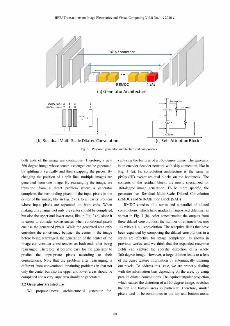
both ends of the image are continuous. Therefore, a new

360-degree image whose center is changed can be generated

by splitting it vertically and then swapping the pieces. By

changing the position of a split line, multiple images are

generated from one image. By rearranging the image, we

transition from a direct problem where a generator

completes the surrounding pixels of the input pixels in the

center of the image, like in Fig. 2 (b), to an easier problem

where input pixels are separated on both ends. When

making this change, not only the center should be completed,

but also the upper and lower areas, like in Fig. 2 (c), since it

is easier to consider consistencies when conditional pixels

enclose the generated pixels. While the generated area only

considers the consistency between the center in the image

before being rearranged, the generation of the center of the

image can consider consistencies on both ends after being

rearranged. Therefore, it become easy for the generator to

predict the appropriate pixels according to their

consistencies. Note that the problem after rearranging is

different from conventional inpainting problems in that not

only the center but also the upper and lower areas should be

completed and a very large area should be generated.

3.2 Generator architecture

We propose a novel architecture of generator for

capturing the features of a 360-degree image. The generator

is an encoder-decoder network with skip-connection, like in

Fig. 3 (a). Its convolution architecture is the same as

pix2pixHD except residual blocks on the bottleneck. The

contents of the residual blocks are newly specialized for

360-degree image generation. To be more specific, the

generator has Residual Multi-Scale Dilated Convolution

(RMDC) and Self-Attention Block (SAB).

RMDC consists of a series and a parallel of dilated

convolutions, which have gradually large-sized dilations, as

shown in Fig. 3 (b). After concatenating the outputs from

three dilated convolutions, the number of channels became

1/3 with a 1 × 1 convolution. The receptive fields that have

been expanded by composing the dilated convolutions in a

series are effective for image completion, as shown in

previous works, and we think that the expanded receptive

fields can capture the specific distortion of a whole

360-degree image. However, a large dilation leads to a loss

of the dense texture information by automatically thinning

out pixels. To address this issue, we are properly dealing

with the information bias depending on the area, by using

parallel dilated convolutions. The equirectangular projection,

which causes the distortion of a 360-degree image, stretches

the top and bottom areas in particular. Therefore, similar

pixels tend to be continuous in the top and bottom areas.

Fig. 3 Proposed generator architecture and components

Fig. 3 Proposed generator architecture and components


38

However, fine objects tend to exist in the center, due to the

decreased effects of the projection. Since a 360-degree

image consists of areas of sparse and dense information, as

in the above case, the adaptive scale of features should be

captured with parallel convolutions. The experiments

conducted to validate the effect of this RMDC are shown in

section 4.3.

SAB is an attention module with architecture similar to

Fig. 3 (c). This makes it possible to refer non-local features

with attention map made by evaluating the correlation

between pixels, which is also used in GANs8). To follow this

step, we are also introducing SAB in order to generate fine

textures. It is placed at the end of residual blocks, since the

effects of referencing similar pixels from the entire feature

map cannot be obtained unless the receptive field is

sufficiently expanded in the previous RMDC and the input

pixels at both ends are referred to in advance. See details in

section 4.

4. Experiments

We used 52,800 images, including the outdoor

categoryof the SUN360 dataset23), as train data and 138

images as test data. We increased train data fourfold through

data augmentation, as shown in sec. 3. The original

resolution of the dataset was 9,104 × 4,552, and we resized

it to 512 × 256. We used 9 RMDC and 1 SAB in the

bottleneck of the generator. In training, the optimizer was

Adam, whose beta_1 was 0.5 and whose beta_2 was 0.999.

In the inference (test), only the generator is used, and the

discriminator is not used. When we visualize the results as a

sphere, we use the software of Ricoh Theta. We used

PyTorch as deep-learning framework.

4.1 Comparison results

Figure 4 shows the comparison of the results. Fig.4 (a),

(b), and (c) show the results of inpainting methods; Fig.4 (d)

and (e) show the results of general image-to-image

translation methods; and Fig.4(f) shows the result of

proposed method. In concrete terms, Fig.4 (a) was made

through context-aware fill on Adobe Photoshop; Fig.4 (b)

and (c) were made through official implementation

models17),18) trained by Places224); Fig.4 (d) and (e) were the

results of the models trained by the SUN360 dataset ;

Fig.4(f) was trained by the SUN360 dataset . The figures in

the second and fourth rows are parts of spherical

visualizations of the generated results of the first and third

rows, respectively.

Inpainting models that do not use 360-degree image as

their datasets cannot generate the specific distortion seen in

360-degree images. Their results are also inconsistent, likely

due to their extremely large completion areas and input

conditions without surrounding pixels. Additionally, pix2pix

and pix2pixHD, which are thought to translate

high-resolution images, generate artifacts in the center of the

results. We think this is because there is a significant

distance from a large generated area to the pixels that can be

referenced as an input condition. Additional consideration is

given in section 4.2. However, our proposed methods can

generate the distortion seen in 360-degree images and fine

texture, suppressing a large artifact.

Fig. 4 Comparison results


39

4.2 Ablation study

Figure 5 shows the results of ablation study for verifying

the effectiveness of the components of the proposed method.

In detail, Fig.5 (a) shows the results of the model when SAB

is removed from the proposed method.

The results have the tendency of carrying the distortion

of a 360-degree image, since it can globally understand what

is seen with RMDC. However, expansion parts show that

generated texture is not fine-grained but blurred.

Additionally, Fig.5 (b) uses the residual block that

consists of two 3×3 convolutions, normalization, and

activation such as pix2pixHD or ResNet25), instead of

RMDC. The number of the blocks is nine, as well as RMDC

of the proposed method. These results show that

self-attention has no effect unless the receptive field is

expanded in advance, while it has the property of selecting

features non-locally. Figure 5 (c) shows the results of the

proposed method, which completes large holes, considering

(a)RMDC (b) SAB (c)RMDC&SAB

Fig. 5 Ablation study

Fig. 6 Visualization of feature maps and comparison results

(a) Parallel only (b) Series only (c) Series-parallel


40

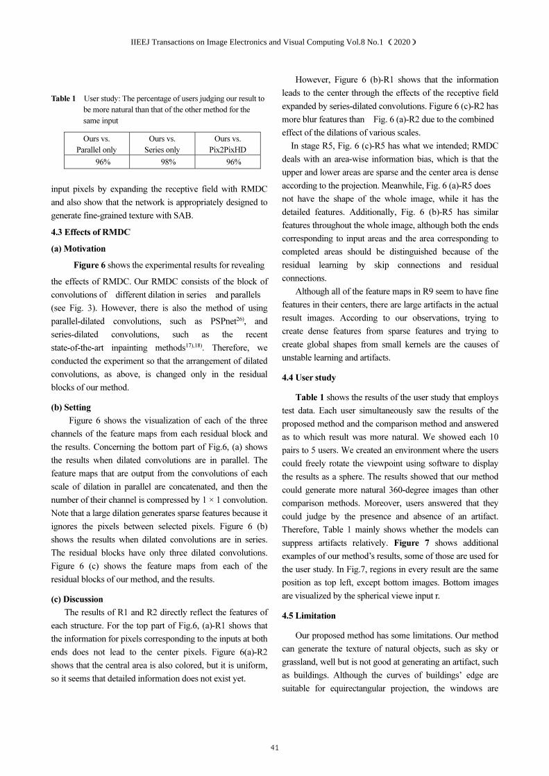
input pixels by expanding the receptive field with RMDC

and also show that the network is appropriately designed to

generate fine-grained texture with SAB.

4.3 Effects of RMDC

(a) Motivation

Figure 6 shows the experimental results for revealing

the effects of RMDC. Our RMDC consists of the block of

convolutions of different dilation in series and parallels

(see Fig. 3). However, there is also the method of using

parallel-dilated convolutions, such as PSPnet26), and

series-dilated convolutions, such as the recent

state-of-the-art inpainting methods17),18). Therefore, we

conducted the experiment so that the arrangement of dilated

convolutions, as above, is changed only in the residual

blocks of our method.

(b) Setting

Figure 6 shows the visualization of each of the three

channels of the feature maps from each residual block and

the results. Concerning the bottom part of Fig.6, (a) shows

the results when dilated convolutions are in parallel. The

feature maps that are output from the convolutions of each

scale of dilation in parallel are concatenated, and then the

number of their channel is compressed by 1 × 1 convolution.

Note that a large dilation generates sparse features because it

ignores the pixels between selected pixels. Figure 6 (b)

shows the results when dilated convolutions are in series.

The residual blocks have only three dilated convolutions.

Figure 6 (c) shows the feature maps from each of the

residual blocks of our method, and the results.

(c) Discussion

The results of R1 and R2 directly reflect the features of

each structure. For the top part of Fig.6, (a)-R1 shows that

the information for pixels corresponding to the inputs at both

ends does not lead to the center pixels. Figure 6(a)-R2

shows that the central area is also colored, but it is uniform,

so it seems that detailed information does not exist yet.

However, Figure 6 (b)-R1 shows that the information

leads to the center through the effects of the receptive field

expanded by series-dilated convolutions. Figure 6 (c)-R2 has

more blur features than Fig. 6 (a)-R2 due to the combined

effect of the dilations of various scales.

In stage R5, Fig. 6 (c)-R5 has what we intended; RMDC

deals with an area-wise information bias, which is that the

upper and lower areas are sparse and the center area is dense

according to the projection. Meanwhile, Fig. 6 (a)-R5 does

not have the shape of the whole image, while it has the

detailed features. Additionally, Fig. 6 (b)-R5 has similar

features throughout the whole image, although both the ends

corresponding to input areas and the area corresponding to

completed areas should be distinguished because of the

residual learning by skip connections and residual

connections.

Although all of the feature maps in R9 seem to have fine

features in their centers, there are large artifacts in the actual

result images. According to our observations, trying to

create dense features from sparse features and trying to

create global shapes from small kernels are the causes of

unstable learning and artifacts.

4.4 User study

Table 1 shows the results of the user study that employs

test data. Each user simultaneously saw the results of the

proposed method and the comparison method and answered

as to which result was more natural. We showed each 10

pairs to 5 users. We created an environment where the users

could freely rotate the viewpoint using software to display

the results as a sphere. The results showed that our method

could generate more natural 360-degree images than other

comparison methods. Moreover, users answered that they

could judge by the presence and absence of an artifact.

Therefore, Table 1 mainly shows whether the models can

suppress artifacts relatively. Figure 7 shows additional

examples of our method’s results, some of those are used for

the user study. In Fig.7, regions in every result are the same

position as top left, except bottom images. Bottom images

are visualized by the spherical viewe input r.

4.5 Limitation

Our proposed method has some limitations. Our method

can generate the texture of natural objects, such as sky or

grassland, well but is not good at generating an artifact, such

as buildings. Although the curves of buildings’ edge are

suitable for equirectangular projection, the windows are

Table 1 User study: The percentage of users judging our result to

be more natural than that of the other method for the

same input

Ours vs.

Parallel only

Ours vs.

Series only

Ours vs.

Pix2PixHD

96% 98% 96%


41

distorted unnaturally. Moreover, our method cannot restore

a semantic object, such as a car or a human from one part.

To summarize above, it is easier for our method to

generate objects with free shapes but more difficult to

generate specific shapes.

5. Conclusion

In this paper, we tackled the 360-degree image

generation and completion by GANs. We proposed the

novel generator with residual multi-scale dilated

convolutions for dealing with the specific properties of a

360-degree image. In the user study, more than 96 percent of

the results generated by the proposed method were judged to

be more natural than the results of the other methods.

References

1) I. J. Goodfellow, J. P-Abadie, M. Mirza, B. Xu, D. W-Farley, S. Ozair,

A. Courville, Y. Bengio: “Generative Adversarial Nets,” 27, Proc. of

Advances in Neural Information Processing Systems (NIPS2014

(2014).

2) C. Barnes, E. Shechtman, A. Finkelstein, D. B. Goldman: “Patchmatch:

A Randomized Correspondence Algorithm for Structural Image Editing”

ACM Trans. on Graphics (TOG) (Proceedings of SIGGRAPH 2009)

Vol.28, No.3 (2009).

3) F. Yu, V. Koltun: “Multi-Scale Context Aggregation by Dilated

Convolutions,” arXiv:1511.07122, Proc. of International Conference on

Learning Representations(ICLR2016) (2016).

4) A. Radford, L. Metz, S. Chintala: “Unsupervised Representation

Learning with Deep Convolutional Generative Adversarial Networks,”

arXiv:1511.06434, Proc. of International Conference on Learning

Representations (ICLR2016) (2016).

5) T. Karras, T. Aila, S. Laine, J. Lehtinen: “Progressive Growing of

GANs for Improved Quality, Stability, and Variation,”


Representations (ICLR2018) (2018).

6) T. Karras, S. Laine, T. Aila: “A Style-Based Generator Architecture for

Generative Adversarial Networks,” arXiv:1812.04948, Proc. of

Computer Vision and Pattern Recognition (CVPR2019)(2019).

7) T. Miyato, T. Kataoka, M. Koyama, Y. Yoshida: “Spectral

Normalization for Generative Adversarial Networks,”

arXiv:1802.05957, Proc. on International Conference on Learning

Representations(ICLR2018) (2018).

8) H. Zhang, I. Goodfellow, D. Metaxas, A. Odena: “Self-Attention

Generative Adversarial Networks,” arXiv:1805.08318, (2018).

9) A. Brock, J. Donahue, K. Simonyan: “Large Scale GAN Training for

High Fidelity Natural Image Synthesis,” arXiv:1809.11096, (2018).

10) P. Isola, J.-Y Zhu, T. Zhou, A. A. Efros: “Image-to-Image Translation

with Conditional Adversarial Networks,” arXiv:1611.07004, Proc. of

Computer Vision and Pattern Recognition (CVPR2017) (2017).

11) T-C. Wang, M-Y. Liu, J-Y. Zhu, A. Tao, J. Kautz, B. Catanzaro:

“High-Resolution Image Synthesis and Semantic Manipulation with

Conditional GANs,” arXiv:1711.11585, Computer Vision and Pattern

Recognition (2018).

12) J-Y. Zhu, T. Park, P. Isola, Alexei A. Efros: “Unpaired Image-to-Image

Translation using Cycle-Consistent Adversarial Networks,”

arXiv:1703.10593, Proc. of International Conference on Computer

Vision (ICCV2017) (2017).

13) M-Y. Liu, T. Breuel, J. Kautz: “Unsupervised Image-to-Image

Translation Networks,” arXiv:1703.00848, Proc. of Advances in Neural

Information Processing Systems(NIPS2017) (2017).

14) A. A. Efros, W. T. Freeman: “Image quilting for texture synthesis and

transfer,” Proc. of the 28th Annual Conference on Computer Graphics

Fig. 7 Other results of our method under the same setup as Fig. 4.


42

and Interactive Techniques,(SIGGRAPH’01) pp.341 ‒ 346, (2001).

15) A. A. Efros, T. K. Leung: “Texture synthesis by non-parametric

sampling,” Proc. of the Seventh IEEE International Conference on

Computer Vision, 1999, Vol. 2, pp. 1033 ‒ 1038. (1999).

16) D. Pathak, P. Krahenbuhl, J.f Donahue, T. Darrell, A. A. Efros: “Context

Encoders: Feature Learning by Inpainting,” Computer Vision and

Pattern Recognition (2016).

17) S. Iizuka, E. S-Serra, H. Ishikawa: “Globally and Locally Consistent

Image Completion,” ACM Trans. on Graphics Vol.36, No.4, (Proc. of

SIGGRAPH) (2017).

18) J. Yu, Z. Lin, J. Yang, X. Shen, Xin Lu, T. S. Huang: “Generative

Image Inpainting with Contextual Attention,” Proc. of Computer Vision

and Pattern Recognition 2018, pp. 5505-5514 (CVPR2018) (2018).

19) N. Kimura, J. Rekimoto: “ExtVision: Augmentation of Visual

Experiences with Generation of Context Images for a Peripheral Vision

Using Deep Neural Net-work,” Proc. of the 2018 CHI Conference on

Human Factors in Computing Systems (CHI ‘18) No. 427, pp. 1–10

(2018).

20) Y-C. Su, K. Grauman: “Learning Spherical Convolution for Fast

Features from 360° Imagery,” arXiv:1708.00919, Proc. of Advances in

Neural Information Processing Systems (NIPS2017) (2017).

21) T. S. Cohen, M. Geiger, J. Koehler, M. Welling. “Spherical CNNs,”


Representations (2018).

22) K.Tateno, N. Navab, F. Tombari: “Distortion-Aware Convolutional

Filters for Dense Prediction in Panoramic Images,” Proc. of European

Conference on Computer Vision (ECCV 2018) pp 732–750 (2018).

23) J. Xiao, K. A. Ehinger, A. Oliva, A. Torralba: “Recognizing scene

viewpoint using panoramic place representation,” Proc. of Computer

Vision and Pattern Recognition (CVPR2012) (2012).

24) B. Zhou, A. Lapedriza, A. Khosla, A. Oliva, A. Torralba: “Places: A 10

million image database for scene recognition, ” IEEE Trans. on Pattern

Analysis and Machine Intelligence Vol.40, No.6, pp.1452–1464 (2017).

25) K. He, X. Zhang, S. Ren, J. Sun: “Deep Residual Learning for Image

Recognition,” arxiv:1512.03385, Computer Vision and Pattern

Recognition(CVPR2016) (2016).

26) H. Zhao, J. Shi, X. Qi, X. Wang, J. Jia: “Pyramid Scene Parsing

Network,” Proc. of Computer Vision and Pattern Recognition

(CVPR2017) (2017).

(Received April 26, 2019)

(Revised August 26, 2019)

Naofumi AKIMOTO

He received M.S from Keio University, Japan.

Yoshimitsu AOKI (Member)

He received the B.E, the M.E. and the Dr.E in Applied Physics all from Waseda University in 1996, 1998, 2001 respectively. He is currently a Professor at the Department of Electrical Engineering of Keio University. His research interests have been in imageprocessing, computer vision, pattern recognition and artificial intelligent system.


43

IIEEJ Paper

Multi-Class Dictionary Design Algorithm Based on Iterative Class

Update K-SVD for Image Compression

Ji WANG†, Yukihiro BANDOH††, Atsushi SHIMIZU†††, Yoshiyuki YASHIMA†(Member)

†Graduate School of Information and Computer Science, Chiba Institute of Technology ,††NTT Media Intelligence Laboratories, NTT Corporation , †††NTT TechnoCross Corporation

<Summary> K-SVD (K-Singular Value Decomposition) is a popular technique for learning a dictionary

that offers sparse representation of the input data, and has been applied to several image coding applications.

It is known that K-SVD performance is largely dependent on the features of the training images. Therefore, a

multi-class dictionary approach is appropriate for natural images given the variety of their features. However,

most published investigations of multi-class dictionaries are based on predetermined classification and do not

consider the relation between classification stage and dictionary training stage. Therefore, there is still room

for improving coding efficiency by linking dictionary training with classification optimization. In this paper,

we propose a multi-class dictionary design method that repeats the following two stages: class update stage

for all training vectors and dictionary update stage for each class by K-SVD. Experiments indicate that the

proposed method outperforms the conventional alternatives as it achieves, for the fixed classification task,

BD-bitrate scores of 6% to 48% and the BD-PSNR value of 0.4 dB to 1.6 dB.

Keywords: image coding, sparse coding, K-SVD, OMP, multi-class

1. Introduction

Image coding technology is one of the key technolo-

gies for communication services, broadcasting and many

storage devices. JPEG and H.264/AVC are widely used

for many currently provided image and video services.

H.265/HEVC, the latest international standard, is also

spreading as a coding scheme for ultra-high resolution

video. Most of the conventional image coding stan-

dards adopt transforms based on discrete cosine trans-

form (DCT). This is because DCT gives a good approx-

imation of the Karhunen-Loeve transform (KLT) under

the condition that there is high correlation among neigh-

boring pixels, which is a known statistical property of

many natural images and videos. However, DCT is not

efficient enough to well represent local features of each

image.

Recent research effort has been devoted to learning

dictionaries that allow image coding to utilize adap-

tive transforms. One of the efficient methods to design

such dictionaries is K-SVD (K-Singular Value Decompo-

sition)1). Given an image signal, K-SVD can derive a dic-

tionary that well approximates each block with a sparse

combination of atoms from the set of blocks composing

the image. An example of this approach is the facial im-

age codec based on the K-SVD dictionary introduced by

Reference 2).

It is known that dictionaries generated by K-SVD are

largely dependent on the features of the training images.

Therefore, the extension of K-SVD to support multiple

dictionaries is a promising approach to more efficient

representations of natural images with various features.

Here, let us call the extended K-SVD “multi-class K-

SVD”. Multi-class K-SVD adaptively selects the most

suitable dictionary based on the local feature(s) of the

image to be encoded.

In order to design multiple dictionaries, it is necessary

to classify the learning data available in terms of charac-

teristics. Various approaches such as edge directionality

and pixel value variance have been studied as local fea-

tures suitable for classification. As examples for image

coding application, some classification methods based on

intra prediction mode and intra/inter prediction residual

power of the coding unit in H.264/AVC or H.265/HEVC

have been already studied3),4).

It has been clarified that multi-class K-SVD gives bet-

ter coding performance than single class K-SVD (i.e. with

one dictionary). However, conventional studies on multi-

class K-SVD use predetermined classification schemes for

dictionary design, and do not consider the relationship


44

between the classification stage and the dictionary train-

ing stage. Therefore, there still remains the potential for

improvements in coding efficiency by combining dictio-

nary training and classification optimization. In this pa-

per, we propose a multi-class K-SVD method that takes

into account the interplay between classification and dic-

tionary design. The proposed method iterates the classi-

fication of training samples and dictionary design for each

class.

The rest of this paper is organized as follows. A survey

of K-SVD and conventional studies on multi-class K-SVD

approaches is given in section 2. The new multi-class K-

SVD algorithm with its class update cycle is proposed

in section 3, and its application to image encoding and

decoding is also described. Analyses of the designed dic-

tionaries and experimental results for image coding are

given in section 4 to demonstrate the effectiveness of the

proposed algorithm. Finally, concluding remarks and fu-

ture works are given in section 5.

2. Previous Work

2.1 Review of K-SVD

In this section, we review the dictionary learning pro-

cedure based on K-SVD1). The set of sample vectors

for dictionary learning is indicated as the matrix Y,

and each column of Y corresponds to N sample vectors

yi(i = 1, 2, · · · , N). For image representation, yi is often

set as a vector whose elements are the pixel values in the

i-th small block obtained after dividing the image. Let

dk(k = 1, 2, · · · ,K) be the k-th atom vector, and let dic-

tionary D be a matrix in which these atoms are arranged

as columns. The dimension of these atoms equals that

of yi. We represent signal yi as a linear combination of

these atoms as expressed by Eq. (1).

yi =K∑

k=1

xikdk (1)

xik, which denotes the k-th element of vector xi, is

the representation coefficient of the sample yi. Using

coefficient matrix X = (x1,x2, · · · ,xN ), Eq. (1) can be

written as

Y ≈ DX . (2)

We consider an optimization problem with sparsity con-

straints that expresses input vector yi with as few atoms

as possible. Approximations with greater sparsity and

smaller error can generally be obtained by using a dictio-

nary learned from samples having characteristics similar

to the samples to be represented. Therefore, it is desir-

able to co-optimize both dictionary D and coefficient X.

This problem can be formulated as

minD,X

||Y −DX||2F subject to ∀i, ||xi||0 ≤ T0 . (3)

Here, notation ‖·‖F stands for the Frobenius norm , ‖xi‖0means the number of non-zero elements in the vector xi,

and T0 is the sparsity constraint threshold.

K-SVD solves Eq.(3) by iterating two stages, sparse

coding stage and dictionary update stage. The former ap-

plies orthogonal matching pursuit (OMP)5) to determine

xi for each yi while fixing D; and the latter updates D

together with the nonzero coefficients of xi. The algor-

ithmic description of K-SVD is detailed in Reference 1).

2.2 Feature specific multiple dictionaries

When an image is expressed under the condition that

the number of non-zero coefficient is T0 or less, the dic-

tionary designed by K-SVD under the constraint that the

number of non-zero coefficients is less than T0 using that

image can minimize reconstruction errors. However, the

characteristics of K-SVD derived dictionaries are highly

dependent on the feature of the images used in train-

ing. A dictionary trained for a specific image is opti-

mum for that image, but not necessarily for other images.

Figure 1 shows the dictionaries Dbarbara, Dlena and

Dpepper designed by K-SVD under the constraint con-

dition of T0 = 3 for each of the three images “Barbara”,

“Lena” and “Pepper”. The atoms included in each dic-

tionary reflect the characteristics of the image used for

training. For example, in the Barbara image, stripe pat-

terns having various directions present in the original im-

age strongly appear as several atoms in the dictionary. To

measure the sparse representation performance of these

dictionaries, the Peak Signal to Noise Ratio (PSNR) val-

ues of the images reconstructed by applying the three

dictionaries Dbarbara, Dlena, and Dpepper to each im-

age, “Barbara”, “Lena”, and “Pepper” are shown in Ta-

ble 1. Table 1 shows the results under the same spar-

sity condition of T0 = 3. The quantization and entropy

coding for coefficients are not applied because they af-

fect the evaluation of sparse representation performance

itself. Therefore, note that the PSNR in Table 1 indi-

Table 1 PSNR values of the images reconstructed bythe different dictionaries

DBarbara DLena DPeppers DHEVC-DCTBarbara 29.59 25.53 25.08 26.20

Lena 31.70 32.95 32.27 29.51

Peppers 31.70 32.31 32.94 29.67


45

cates the sparse representation performance, not coding

performance. That is, first, three non-zero coefficients

are obtained by repeating the projection (OMP) of the

target block vector in the image onto the basis in each

dictionary three times. After that, the target image is re-

constructed using only those three coefficients, and how

much it can approximate the original image was mea-

sured. For comparison, the result when each image is re-

constructed using the HEVC-DCT6)dictionary under the

same sparsity condition of T0 = 3 is also shown. For

all images, image reconstruction performance is highest

with the dictionary trained against itself. Unfortunately,

using a dictionary trained against different images seri-

ously degrades image reconstruction performance. For

example, for the Barbara image, the other two K-SVD

dictionaries yield worse performance than HEVC-DCT.

When applying K-SVD to image coding, the decoder has

to use the same dictionary as the encoder, so the de-

signed dictionary itself must be encoded and transmitted

to the decoder. However, the coding and transmission of

atoms for each image every time incurs large overheads

for information transmission, and is not practical from

the viewpoint of rate distortion performance.

To solve this problem, some researchers take ap-

proaches that share the multiple dictionaries among an

encoder and a decoder in advance. That is, first, the im-

age is divided into small blocks to calculate local features,

then a set of blocks having similar features is created as

a class, and finally, K-SVD is executed for each class so

as to create multiple dictionaries. It is considered that

the local features in images can be classified into simi-

lar geometric patterns such as the direction of edges and

texture features. A set of dictionaries designed for each

class is shared in advance by the encoder and decoder,

and these are adaptively switched when encoding. This

eliminates the need to encode new sets of dictionary in-

formation, and makes it possible to represent more im-

ages efficiently. For example, in Reference 3), based on

the H.265/HEVC framework, an approach is proposed in

which training samples are classified by transform unit

(TU) size and a dictionary is designed by K-SVD for

each class. Moreover, it is described that an application-

specific dictionary can be developed for particular ap-

plications such as gaming or medical video by changing

samples in training. Further, in Reference 4), block classi-

fication based on intraframe/interframe prediction resid-

ual power is performed using the H.264/AVC framework,

and different dictionaries are designed class by class. For

(a) (b)

(c) (d)

(e) (f)

Fig. 1 Dictionaries designed by K-SVD; the original im-ages ( (a), (c), (e) ) and their corresponding dic-tionaries ( (b), (d), (f) )

application other than image coding, multiple dictionar-

ies designs based on K-SVD also have been studied. In

reference 7), multiple dictionaries are designed in order to

sharpen the character image. Small patches in images are

classified into 13 classes based on their pixel distribution

state, and a K-SVD dictionary is designed for each class.

In Reference 8), the effectiveness of class specific sparse

codes is investigated in the context of discriminative ac-

tion classification. The local motion features for each

action are trained by K-SVD to design the action specific

dictionary. In References 3),4),7) and 8), local regions of

an image are classified into multiple classes according to

their characteristics, and a dictionary setting based on K-

SVD is performed class by class. However, conventional

methods do not consider the effects of classification on

the subsequent processes, a dictionary learning based on

K-SVD, because these methods use pre-determined fea-

tures in performing classification. This is, the classifica-

tions and dictionary learning are designed independently.

This raises the disadvantage that image representation

performance depends on what kinds of features are used

for classification.


46

pi = argminc

Ec

Ec = ‖yi −Dcxc

i‖2F

Ypi = Ypi + {yi}

Ypi = Ypi − {yi}

pi = pi

E1

E2

EC

D1x1

i

D2x2

i

DCxC

i

DC

D2

D1Y1

Y2

YC

Y

Yc =⋃

pi=c

{yi}

......

......

yi

Y = {yi|i = 1, 2, · · · , N}

Fig. 2 Block diagram of dictionary training by Multi-class K-SVD

For example that considers the effect of classification

on dictionary learning based on K-SVD, there are some

studies on image clustering. In References 9) and 10), a

dictionary for face recognition and object recognition are

designed by K-SVD. They improved the performance of

class identification by adding not only the approximation

error for the training data but also the identification er-

ror based on the linear classifier to the cost function of

the K-SVD algorithm. The dictionary designed by the

methods in References 9) and 10) is a “single” dictionary

for better class classification and does not correspond to

the multi-class dictionary design handled in this paper.

In Reference 11), the design method of class specific dic-

tionary for clustering is proposed. The dictionaries, co-

efficients, and the parameters of support vector machine

(SVM) are designed based on an alternating optimal ap-

proach for the training data. The purpose in Reference

11) is not a dictionary design for image compression, but a

dictionary design for image classification. For this reason,

the correct class label information is added to the train-

ing data used for dictionary design as supervised data.

Therefore, the method proposed in Reference 11) cannot

support unsupervised learning. Furthermore, since each

atom is not occupied by a specific class dictionary but

is shared among the dictionaries of multiple classes, the

designed dictionaries are not completely independent for

each class.

In contrast to the conventional research described

above, the contribution of this paper is to propose a

multi-class dictionary design method targeting image

coding, and to clarify the effect of the proposed method.

In order to focus on application to image coding, its clas-

sification takes an unsupervised approach based on the

k-means method, unlike the conventional supervised tech-

nique for such as object recognition and image classifica-

tion. In the proposed method, a multi-class dictionary is

designed by repeating the two stages, unsupervised class

update stage for all training vectors and dictionary up-

date stage for each class by K-SVD. Compared to con-

ventional approaches that do not perform classification

optimization, better compression efficiency is expected.

3. Proposed Method

In this section, we propose a new multi-class dictio-

nary design method consisting of two stages (dictionary

design and classification), and its application for image

coding. For designing multi-class dictionaries, we iter-

ate the classification of training data and the dictionary

design process for each class. By performing iterative

convergence processing, we can create multi-class dictio-

naries that solve the conventional problem of what kind

of local features should be used for clustering. In the pro-

posed method in this paper, dictionary design including

classification of training data is performed as unsuper-

vised learning. Therefore, our method includes a different

process from the conventional dictionary design method

based on iterative updating using supervised data. In this

section, we show the detail algorithm to design the mul-

tiple dictionaries based on K-SVD under unsupervised

training and how to apply multi-class dictionaries ob-


47

Algorithm 1 The multi-class K-SVD algorithm

Initialization:Set the number of classes C. Set the maximum number ofiterations for class update Lmax . Set over-complete DCT toinitial Dc for each class. Classify all training vectors yi(i =1, 2, . . . , N) into classes based on DSIFT, Yc =

⋃pi=c{yi}

and set class index for yi to pi. Set count = 0.

Dictionary update stage:for c = 1, 2, · · · , C do

Calculate dictionary Dc with K-SVD.end for

Class update stage:for i = 1, 2, · · · , N do

for c = 1, 2, · · · , C dofind xc

i that approximates yi by sparse coding with Dc

end fornew class index pi = argminc ‖yi −Dcxc

i‖2Fif pi �= pi then

Ypi = Ypi + {yi}Ypi = Ypi − {yi}pi = pi

end ifend forSet count = count + 1

Convergence check:if count > Lmax or no class index is changed then

return Dictionary Dc(c = 1, 2, . . . , C).else

Back to “Dictionary update stage”.end if

tained by the proposed method to image compression.

3.1 Dictionary training process

Figure 2 depicts the process flow of the proposed

multi-class K-SVD dictionary design method. Since dic-

tionary design and classification cannot be optimized at

the same time, the proposal alternately performs, for each

class, the classification of training data and dictionary

design. Algorithm 1 details the steps of the multi-class

dictionary design; the specific procedures in each stage

are described as follows.

First, training images are divided into small blocks,

and training vectors are calculated to yield a set of m-

dimensional vectors yi(i = 1, 2, . . . , N) where elements

of yi are pixel values in the i-th block. N is the num-

ber of training vectors. We consider that each train-

ing vector, yi, can be approximated as a weighted lin-

ear combination of the atoms in dictionary Dc, where

the weight coefficients of the atoms are denoted as coef-

ficient vector xi. Training vectors are initially classified

into C classes, Y1,Y2, · · · ,YC , based on their local fea-

tures and class index for yi is determined as pi, where

pi ∈ {1, 2, 3 . . . C}. As the local feature, dense scale in-

variant feature transform (DSIFT)12)is utilized because

the distribution of edge gradient direction in a block can

be expected to significantly influence the shape of basis

patches to be designed. The initial dictionary for each

class is set to over-complete DCT with size K.

Next, in the dictionary update stage, a dictionary that

enables sparse representation for training vectors for each

class is designed. In preparation, we concatenate all

training vectors yi that belong to class c as columns of

matrix Yc ∈ Rm×n(c) and similarly concatenate coeffi-

cient vectors xi for yi to build matrix Xc ∈ RK×n(c).

Here, n(c) is the number of training vectors belonging

to the c-th class. Dictionary Dc and coefficient Xc are

obtained by solving Eq. (4).

minXc,Dc

‖Yc −DcXc‖2F , s.t. ∀i, ‖xci‖0 ≤ T0 (4)

As the solver of the problem in Eq. (4), we use K-

SVD. Specifically, as shown in Eq. (4), dictionary Dc ∈Rm×K and coefficients Xc that minimize the square error

between original signal Yc and its reconstructed signal

DcXc are found under the sparsity constraint that the

number of nonzero coefficients in each column of matrix

Xc is equal to or less than T0. This designs C dictionaries.

After dictionary design, the class update stage is exe-

cuted. Among the C kinds of dictionaries Dc, a new class

index pi for each training vector yi is re-assigned so as to

satisfy the following:

pi = argminc ‖yi −Dcxci‖2F

s.t. ‖xci‖0 ≤ T0, i = 1, 2, · · · , N.

(5)

The above equation yields the class index that mini-

mizes the square error between a training vector and its

reconstructed vector from the designed dictionary subject

to the constraint on the number of nonzero coefficients.

If pi is different from pi, the training sample yi is moved

to class Ypi and the class index pi of yi is replaced by pi.

These two steps, the dictionary update stage for each

class by K-SVD and the class update stage, are iterated

until the convergence conditions are satisfied. The con-

vergence conditions are that the number of iterations ex-

ceeds predetermined threshold Lmax or that none of the

class indices of the training vectors change. Finally, the

algorithm outputs Dc(c = 1, 2, · · · , C) as the multi-class

dictionaries.

In order to effectively represent the actual image, each

dictionary to be designed should contain one DC basis,

as has been confirmed 1)13). Therefore, one DC basis is

included in the initial dictionary for each class, and the

DC basis is not changed during iterative processing. Also,


48

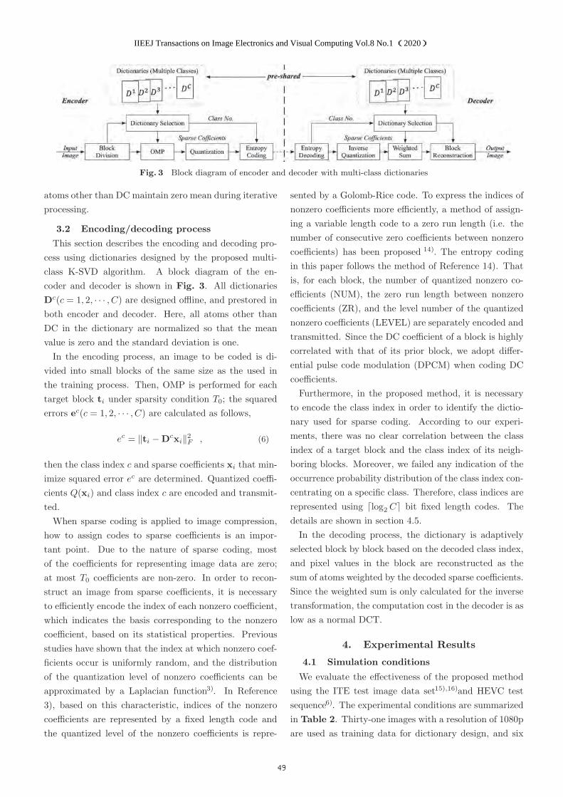
Fig. 3 Block diagram of encoder and decoder with multi-class dictionaries

atoms other than DC maintain zero mean during iterative

processing.

3.2 Encoding/decoding process

This section describes the encoding and decoding pro-

cess using dictionaries designed by the proposed multi-

class K-SVD algorithm. A block diagram of the en-

coder and decoder is shown in Fig. 3. All dictionaries

Dc(c = 1, 2, · · · , C) are designed offline, and prestored in

both encoder and decoder. Here, all atoms other than

DC in the dictionary are normalized so that the mean

value is zero and the standard deviation is one.

In the encoding process, an image to be coded is di-

vided into small blocks of the same size as the used in

the training process. Then, OMP is performed for each

target block ti under sparsity condition T0; the squared

errors ec(c = 1, 2, · · · , C) are calculated as follows,

ec = ‖ti −Dcxi‖2F , (6)

then the class index c and sparse coefficients xi that min-

imize squared error ec are determined. Quantized coeffi-

cients Q(xi) and class index c are encoded and transmit-

ted.

When sparse coding is applied to image compression,

how to assign codes to sparse coefficients is an impor-

tant point. Due to the nature of sparse coding, most

of the coefficients for representing image data are zero;

at most T0 coefficients are non-zero. In order to recon-

struct an image from sparse coefficients, it is necessary

to efficiently encode the index of each nonzero coefficient,

which indicates the basis corresponding to the nonzero

coefficient, based on its statistical properties. Previous

studies have shown that the index at which nonzero coef-

ficients occur is uniformly random, and the distribution

of the quantization level of nonzero coefficients can be

approximated by a Laplacian function3). In Reference

3), based on this characteristic, indices of the nonzero

coefficients are represented by a fixed length code and

the quantized level of the nonzero coefficients is repre-

sented by a Golomb-Rice code. To express the indices of

nonzero coefficients more efficiently, a method of assign-

ing a variable length code to a zero run length (i.e. the

number of consecutive zero coefficients between nonzero

coefficients) has been proposed 14). The entropy coding

in this paper follows the method of Reference 14). That

is, for each block, the number of quantized nonzero co-

efficients (NUM), the zero run length between nonzero

coefficients (ZR), and the level number of the quantized

nonzero coefficients (LEVEL) are separately encoded and

transmitted. Since the DC coefficient of a block is highly

correlated with that of its prior block, we adopt differ-

ential pulse code modulation (DPCM) when coding DC

coefficients.

Furthermore, in the proposed method, it is necessary

to encode the class index in order to identify the dictio-

nary used for sparse coding. According to our experi-

ments, there was no clear correlation between the class

index of a target block and the class index of its neigh-

boring blocks. Moreover, we failed any indication of the

occurrence probability distribution of the class index con-

centrating on a specific class. Therefore, class indices are

represented using �log2 C� bit fixed length codes. The

details are shown in section 4.5.

In the decoding process, the dictionary is adaptively

selected block by block based on the decoded class index,

and pixel values in the block are reconstructed as the

sum of atoms weighted by the decoded sparse coefficients.

Since the weighted sum is only calculated for the inverse

transformation, the computation cost in the decoder is as

low as a normal DCT.

4. Experimental Results

4.1 Simulation conditions

We evaluate the effectiveness of the proposed method

using the ITE test image data set15),16)and HEVC test

sequence6). The experimental conditions are summarized

in Table 2. Thirty-one images with a resolution of 1080p

are used as training data for dictionary design, and six


49

Table 2 Experimental conditions

Dictionarytraining

Block size 8× 8Initial dictionary Over-complete DCT

with 16× 16 atomsNumber of classes C 32, 64, 128Sparsity parameter T0 3, 5, 7, 9Initial classifier k-means

using DSIFT12)

Maximum iterationlimit for class update,Lmax

20

Encoding

Coefficientsquantization

Uniform quantiza-tion for step QP (forDC, QP=1)

Coefficients coding(DC)

DPCM using theprevious block’s DCcoefficient

Coefficients coding(AC)

Separately encodingof NUM, ZR, andLEVEL

Class index Fixed length coding

(a) BasketballDrive (b) BQTerrace

(c) Cactus (d) ChristmasTree

(e) Kimono1 (f) ParkScene

Fig. 4 Test images

images in Fig. 4, not included in the training images, are

used as encoding targets.

In this experiment, in order to analyze the behavior

of the proposed method in detail, multi-class dictionar-

ies are designed using various parameters. Specifically,

we prepared dictionaries by setting the class index C

to 32, 64, 128 and the sparsity parameter T0 to 3, 5, 7, 9.

Each basis included in the dictionary is set to 8× 8 size,

following JPEG. Dictionary training based on multi-class

K-SVD is started for each class by setting overcomplete

DCT with 16 × 16 = 256 atoms as an initial dictionary.

For the initial classification, the DSIFT feature obtained

for each block is used, and the maximum number of iter-

ations of class update is set to 20.

Next, experimental conditions of encoding are as fol-

lows. The coding experiment examined intraframe cod-

ing, and performance is evaluated from the viewpoint of

the PSNR of the decoded image and the amount of in-

formation transferred. After the image to be coded is

divided into 8 × 8 blocks, sparse coding using a multi-

class dictionary is performed for each block according to

the method described in section 3.2, and a class index for

specifying the dictionary to be used and the coefficients

corresponding to each basis are obtained. As described in

section 3.2, DC coefficients of two neighboring blocks are

strongly correlated, so the difference from the decoded

DC coefficient of the previous block is quantized and en-

coded. Since the DC coefficient greatly influences visual

image quality, the quantization step for the DC coefficient

difference is set to just one. The amount of information

for DC coefficients is calculated as the entropy of the

quantization level number corresponding to the quantized

prediction error. AC coefficients (coefficients for atoms

other than DC) are linearly quantized with quantization

width QP. The quantization level number “LEVEL” for

coefficient x is calculated as

LEVEL = sign(x)× (|x|+QP/2)/QP . (7)

The amount of information for AC coefficients is cal-

culated as the entropy obtained from the occurrence

probability NUM, ZR and LEVEL. Fixed length code

of �log2 C� is allocated to each class index. The total

amount of information required for each block is calcu-

lated as the sum of the amount of information occupied

by DC coefficient, AC coefficients, and class index.

4.2 Dictionary training performance

Figure 5 shows the percentage of training samples

whose class indices changed among the training samples

with each class update iteration. Clearly, the change in

the number of training samples belonging to each class

gradually converges to zero with class update iteration

regardless of the number of classes, C, or the sparsity

parameter, T0.

In addition, Fig. 6 shows the mean square error (MSE)

between the original block and the block reconstructed by

the dictionary designed after each iteration number. In

this determination, coefficient quantization was not per-

formed. From Fig. 6, we find that MSE strongly decreases

in the first few iterations, continues to gradually decrease

subsequent class update iterations, and converges to a ba-


50

(a) T0 = 3 (b) T0 = 5

(c) T0 = 7 (d) T0 = 9

Fig. 5 The rate of change in the number of training sam-ples belonging to each class

(a) T0 = 3 (b) T0 = 5

(c) T0 = 7 (d) T0 = 9

Fig. 6 MSE convergence characteristics for the trainingdata

sically constant value in 15 to 20 iterations regardless of C

or T0. Furthermore, the converged value of MSE appar-

ently decreases as class number C increases and as spar-

sity parameter T0 increases. This is because the atoms

that offer better approximation of the local pixel value

distribution are easier to find in the designed dictionar-

ies as C and/or T0 increase. Based on the above results,

the following experiments were carried out by setting the

maximum iteration number for class update, Lmax , to 20.

(a) Number of the training samples

(b) MSE(per pixel)

Fig. 7 The number of training samples belonging toeach class and their sparse representation MSE

Figure 7 shows the number of training samples be-

longing to each class and the MSE obtained by sparsely

approximating those training samples using T0 = 3 and

C = 32. The blue bar in Fig. 7 shows MSE of initial

classification and the red bar shows MSE after 20 iter-

ations. In the initial classification based on DSIFT, the

training sample distribution concentrates on some classes,

but training samples are distributed among many classes

with each class update iteration. For classes whose ini-

tial classification have large MSEs, it is found that after

20 class updates the MSE decreases dramatically. It is

also found that sparse approximation yields an inverse

correlation between the number of samples belonging to

each class and MSE. This is because among the training

image data, as the ratio of the low frequency vector rises

above that of the high frequency vector, and the vector

frequency falls, the reconstruction error becomes smaller.

This tendency was also found in experiments using other

numbers of classes or other sparsity parameters.

4.3 Initial classifier

DSIFT is based on an edge gradient histogram over ori-

entation bins, and the atoms in the designed dictionary of

each class can reflect the edge shape feature of the origi-

nal block. In this subsection, we investigate how the con-

vergence value and the convergence speed differ depend-

ing on the initial classification in the proposed algorithm.


51

Two classification methods, block-variance-based method

(VAR) and random-assignment-based method (RAND),

other than DSIFT were tested. Block variance is a mea-

sure of the spread of pixel values in a block, reflecting the

sharpness and complexity of the edge. It is calculated by

the following equation:

VAR =∑

i

∑

j

(f(i, j)−M)2 , (8)

where M is the average of pixel values in the block. For

the initial classification, the blocks are classified into C

classes by k-means method based on VAR. RAND is a

method to assign C random variables of 1 to C as class

numbers for each block, and it does not require any spe-

cific feature calculations. The experiment by RAND is in-

tended to verify how the proposed method behaves when

starting from random initial classification.

We designed three types of multiclass dictionaries un-

der three initial classifications, DSIFT, VAR, and RAND.

Figure 8 shows the convergence characteristics of MSE

when C = 32 and T0 = 5. From Fig. 8, it can be seen

that the dictionaries designed by initial classification with

RAND without class update (i.e. the first K-SVD out-

0 5 10 15 20Number of iterations

6.5

7

7.5

8

8.5

MS

E p

er p

ixel

DSIFTRandomVariance

Fig. 8 Convergence characteristics based on three kindsof initial classification methods

put dictionaries) have poor image representation perfor-

mance. Moreover, MSE by the dictionaries designed by

the initial classification by DSIFT becomes smaller than

that by VAR. Moreover, regardless of which initial clas-

sification is used, MSE decreases and converges as the

number of iterations increases. The three MSEs converge

to almost the same value, but the convergence speed is

the fastest for DSIFT. The similar tendency has shown by

the measurement of convergence characteristics based on

three kinds of initial classification methods under various

C and T0. From these results, it can be concluded that

the proposed algorithm can design the high performance

multiclass dictionaries regardless of initial classification

method if the number of class update iterations is suffi-

ciently large.

4.4 Coding performance

This section examines the rate distortion characteris-

tics to evaluate the performance of our approach.

Table 3 details the performance (Bjontegaard metric)

of the proposed method17) at different C and T0 values.

In generating the data, the proposed method used dic-

tionaries designed with 20 iterations, while the reference

method to be compared used dictionaries designed un-

der initial classification. As described later, there is an

appropriate T0 in the range of the target bit rate (com-

pression ratio). In other words, a small T0 is effective for

an application used in a low bit rate environment, and

a large T0 is effective for an application used in a high

bit rate environment. Also, there is an appropriate C

depending on the implementation environment of the en-

coder/decoder. In other words, if the memory available

to the encoder and decoder is large, we can use dictionar-

ies designed with a large C, but if the memory is small,

Table 3 BD-PSNR[dB] and BD-rate[%] of the proposed method against the conventional method without class updateunder the same C and T0 as an anchor

T0 CBasketballDrive BQTerrace Cactus ChristmasTree Kimono1 ParkScenePSNR RATE PSNR RATE PSNR RATE PSNR RATE PSNR RATE PSNR RATE

32 0.85 -26.27 0.75 -26.32 0.78 -22.64 0.83 -40.58 0.67 -8.46 0.75 -17.273 64 1.07 -32.27 0.95 -32.81 1.01 -29.59 0.95 -45.09 1.01 -13.15 0.9 -20.33

128 1.03 -30.56 0.92 -30.75 0.99 -28.49 1.01 -48.26 0.98 -11.96 0.95 -21.23

32 0.79 -17.49 0.69 -17.17 0.75 -15.96 0.91 -26.59 0.43 -5.81 0.77 -12.975 64 1.2 -25.88 1.02 -24.57 1.13 -23.61 1.16 -32.75 0.97 -14.06 1.05 -17.43

128 1.12 -23.83 0.99 -23.6 1.09 -22.26 1.23 -34.7 0.92 -12.72 1.05 -17.32

32 0.84 -16.78 0.68 -15.03 0.77 -14.47 0.99 -22.2 0.46 -7.17 0.79 -12.127 64 1.23 -23.56 1.04 -21.8 1.21 -21.97 1.35 -28.93 0.81 -12.07 1.18 -17.36

128 1.16 -22.07 0.99 -20.35 1.13 -20.29 1.34 -28.3 0.89 -13.08 1.1 -16.2

32 0.85 -16.27 0.7 -14.62 0.78 -14.24 1.02 -19.56 0.56 -8.83 0.82 -12.29 64 1.13 -20.59 0.99 -19.65 1.1 -19.09 1.4 -25.73 0.46 -6.7 1.18 -16.79

128 1.13 -20.16 1.02 -19.69 1.13 -19.04 1.48 -26.32 0.77 -11.47 1.18 -16.45


52

we can use only dictionaries designed with a small C.

Thus, we can say there are many cases where dictionaries

designed with fixed T0 and C are used, to satisfy the re-

quirements of the encoder/decoder implementation and

application environment. Therefore, in Table 3, C and

T0 of the conventional method used as anchors are the

same as C and T0 of the proposed method, respectively.

As shown in Table 3, regardless of the number of classes

and sparsity parameters, our approach attained signifi-

cantly better BD-PSNR and BD-rate performance than

the conventional approach. From Table 3, it can be seen

that BD-PSNR improved from 0.4 dB to 1.5 dB for vari-

ous images. In addition, the performance improvement in

BD-rate was 6% to 48%, and reducing sparsity parameter

T0 increased the bitrate reduction.

In addition, the performance of the proposed method is

compared with that of the conventional method in which

the encoding is performed with the number of classes that

gives the best performance. First, the dictionaries in the

conventional method are designed by setting the number

of classes to 1, 4, 16, 32, 64, 128, and 256. After that, the

Fig. 9 BD bitrate against C = 1 as an anchor (withoutclass update)

rate-distortion characteristics when encoding with each

dictionary are obtained. Next, using the encoding per-

formance when C = 1 (i.e. single class) as an anchor,

the number of classes, Cbest, with the best BD-rate is

determined for each T0. The result is shown in Fig. 9.

Figure 9 shows the average BD-rate for the six test se-

quences, and almost the same results were also obtained

for individual images. From Fig. 9, we can see that Cbest

is 32. Next, we summarize the BD-PSNR and BD-rate

of the proposed method in Table 4, in which the anchor

is the RD characteristic of the conventional method with

Cbest. Note that since Cbest = 32, the row of C = 32 in

Table 4 has the same value as Table 3. From the above

considerations, it was confirmed that the coding perfor-

mance of the proposed method also exceeded that of the

conventional method using the number of classes which

gives the best performance.

Figure 10 and Fig. 11 show the PSNR and bit rate

of the test image ‘Cactus’ and ‘ParkScene’ measured un-

der the condition of C = 32, 64, and 128. In Fig. 10

and Fig. 11, all results include overhead information for

class indices. Figures 10 (a), (c) and (e) show the rate

distortion characteristics of the proposed method, and

Figs. 10 (b), (d) and (f) show those of the conventional

method. We can confirm the effectiveness of the proposed

method relative to the conventional method under same

C and T0 by comparing Figs. 10(a), (c) and (e), with

Figs. 10 (b), (d) and (f), respectively. Also, note that

Figure 10 (b) is the result of encoding with the number of

classes that gives the maximum performance in the con-

ventional method. We can see that the performances of

the proposed method shown in Figs. 10 (a), (c) and (e),

are superior to the best performance of the conventional

method shown in Fig. 10 (b). A similar discussion is pos-

Table 4 BD-PSNR[dB] and BD-rate[%] of the proposed method against the conventional method without class updateunder the best C(= 32). Note that the values in the row for C = 32 are the same as in Table 3

T0 CBasketballDrive BQTerrace Cactus ChristmasTree Kimono1 ParkScenePSNR RATE PSNR RATE PSNR RATE PSNR RATE PSNR RATE PSNR RATE

32 0.85 -26.27 0.75 -26.32 0.78 -22.64 0.83 -40.58 0.67 -8.46 0.75 -17.273 64 0.92 -27.50 0.80 -27.22 0.82 -23.22 0.88 -41.86 0.74 -9.42 0.80 -17.88

128 0.99 -29.41 0.84 -27.68 0.90 -25.24 0.96 -45.50 0.84 -10.31 0.87 -19.29

32 0.79 −17.49 0.69 −17.17 0.75 −15.96 0.91 −26.59 0.43 −5.81 0.77 −12.975 64 0.78 −16.88 0.66 −15.56 0.71 −14.08 0.88 −25.06 0.42 −5.44 0.74 −12.08

128 0.81 −17.08 0.68 −15.44 0.75 −14.54 0.94 −26.64 0.48 −6.27 0.76 −12.45

32 0.84 −16.78 0.68 −15.03 0.77 −14.47 0.99 −22.20 0.46 −7.17 0.79 −12.127 64 0.73 −13.78 0.64 −12.69 0.68 −11.65 0.95 −20.24 0.35 −4.90 0.71 −10.36

128 0.78 −14.41 0.65 −12.34 0.70 −11.67 0.98 −20.29 0.41 −5.67 0.72 −10.40

32 0.85 −16.27 0.70 −14.62 0.78 −14.24 1.02 −19.56 0.56 −8.83 0.82 −12.209 64 0.66 −11.72 0.60 −11.20 0.63 −10.17 0.92 −16.27 0.40 −5.86 0.68 −9.52

128 0.68 −11.78 0.62 −11.05 0.63 −9.81 0.94 −16.40 0.41 −5.80 0.67 −9.21


53

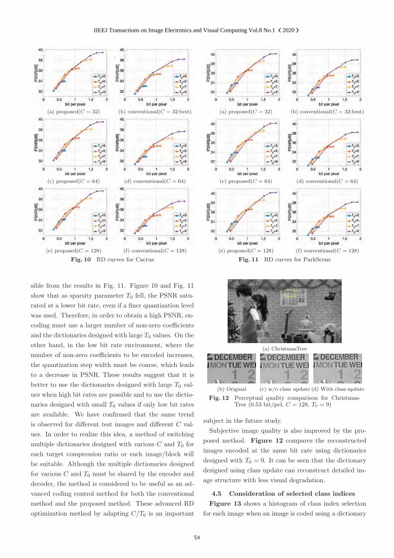
(a) proposed(C = 32) (b) conventional(C = 32:best)

(c) proposed(C = 64) (d) conventional(C = 64)

(e) proposed(C = 128) (f) conventional(C = 128)

Fig. 10 RD curves for Cactus

sible from the results in Fig. 11. Figure 10 and Fig. 11

show that as sparsity parameter T0 fell, the PSNR satu-

rated at a lower bit rate, even if a finer quantization level

was used. Therefore, in order to obtain a high PSNR, en-

coding must use a larger number of non-zero coefficients

and the dictionaries designed with large T0 values. On the

other hand, in the low bit rate environment, where the

number of non-zero coefficients to be encoded increases,

the quantization step width must be coarse, which leads

to a decrease in PSNR. These results suggest that it is

better to use the dictionaries designed with large T0 val-

ues when high bit rates are possible and to use the dictio-

naries designed with small T0 values if only low bit rates

are available. We have confirmed that the same trend

is observed for different test images and different C val-

ues. In order to realize this idea, a method of switching

multiple dictionaries designed with various C and T0 for

each target compression ratio or each image/block will

be suitable. Although the multiple dictionaries designed

for various C and T0 must be shared by the encoder and

decoder, the method is considered to be useful as an ad-

vanced coding control method for both the conventional

method and the proposed method. These advanced RD

optimization method by adapting C/T0 is an important

(a) proposed(C = 32) (b) conventional(C = 32:best)

(c) proposed(C = 64) (d) conventional(C = 64)

(e) proposed(C = 128) (f) conventional(C = 128)

Fig. 11 RD curves for ParkScene

(a) ChristmasTree

(b) Original (c) w/o class update (d) With class update

Fig. 12 Perceptual quality comparison for Christmas-Tree (0.53 bit/pel, C = 128, T0 = 9)

subject in the future study.

Subjective image quality is also improved by the pro-

posed method. Figure 12 compares the reconstructed

images encoded at the same bit rate using dictionaries

designed with T0 = 9. It can be seen that the dictionary

designed using class update can reconstruct detailed im-

age structure with less visual degradation.

4.5 Consideration of selected class indices

Figure 13 shows a histogram of class index selection

for each image when an image is coded using a dictionary


54

(a) BasketballDrive (b) BQTerrace

(c) Cactus (d) ChristmasTree

(e) Kimono1 (f) ParkScene

Fig. 13 Class selection probability (T0 = 3, C = 128)

designed under the condition of C = 128 and T0 = 3.

From Fig. 13, it can be seen that the selection ratio of

classes differs with the image, and that image reconstruc-

tion does trigger switching to the appropriate dictionary

according to the distribution of the local features of the

image to be encoded. Figure 14 shows the relationship

between the feature of the bases included in some dictio-

naries and the feature of the blocks that selected each of

those dictionaries. Figure 14 (a) is a part of image“Park

Scene”. Figure 14 (b), Fig. 14 (d) and Fig. 14 (f) show

the blocks using the dictionaries shown in Fig. 14 (c),

Fig. 14 (e) and Fig. 14 (g), respectively. We can see that

the blocks in Fig. 14 (b), Fig. 14 (d) and Fig. 14 (f) con-

tain vertical, diagonal and horizontal edge, respectively,

and the selected dictionary contains many bases that re-

flect the block feature. These confirm the effectiveness of

the multi-class dictionary approach. Also, since there is

no class index that is rarely used, it can be said that the

number of classes is not excessive.

Next, we consider the local correlation of class indices.

If the class indices of neighboring blocks are highly cor-

related, applying the following rules in code assignment

may reduce the total code length. Let CP be the class

index of the target block, CA be the class index of its left

neighboring block, and CB be the class index of its upper

(a) a part of “Park Scene”

(b) Block corresponding to dictio-nary (c)

(c) Dictionary #25

(d) Block corresponding to dictio-nary (e)

(e) Dictionary #29

(f) Block corresponding to dictio-nary (g)

(g) Dictionary #88

Fig. 14 Example of relationship between the feature ofblocks and the selected dictionary

neighboring block. The code assignment rule is,

� “00” if CP = CA

� “01” if CP = CB

� “1”+“fixed length code with �log2 C� bit” otherwise.

The number of bits yielded by the above rule is smaller

than that yielded by fixed length coding only when the

probabilities of CP = CA or CP = CB are larger than 0.25

(C = 32), 0.2 (C = 64), 0.167 (C = 128), respectively.

We measured the probability that the class index of a

block to be coded is the same as the class index of its

left or upper neighboring blocks for the six test images in

Fig.4 under T0 = 3. They were 0.118, 0.076, 0.054 for the

case of C = 32, C = 64 and C = 128, respectively. This

result suggests that the class index has only slight local

correlation, and that using a variable length code to the

class has little benefit. Therefore, as described in section

3.2, it is appropriate to assign a fixed length code to each


55

class index.

5. Conclusions

This study proposed a multi-class K-SVD method that

considers interdependency of classification performance

and dictionary design. In the proposed method, after

multiple dictionaries are designed by K-SVD, sparse cod-

ing for each training vector is performed using all of the

dictionaries. As a result, the training vector is reclassified

into the class that best approximates it. By iteratively

performing the dictionary design stage and the class up-

date stage, it is possible to design dictionaries that en-

able more efficient sparse representation. Experiments on

still images revealed that the proposed algorithm gives

a significant coding gain compared to the conventional

method based on fixed classification with predetermined

features.

We believe that the proposed method can be further ex-

panded in more directions and also has high potential as

regards research. First, the proposed method can be ex-

tended to multi-class dictionary design for residual signals

of intraframe prediction as used in H.265/HEVC. Con-

sidering its application to videos, it can also be applied

to dictionary design for motion compensation prediction

error. In addition, the class selection strategy under

rate-distortion optimization and the adaptive switching

method of multiple dictionaries which are designed with

different sparse constraint parameters, are considered to

be interesting viewpoints of future research. Moreover,

introducing a dynamic class merge process in the middle

of iterated dictionary design offers attractive research di-

rections for producing more compact sets of dictionaries

that can improve coding efficiency.

References

1) M. Aharon, M. Elad, A. Bruckstein: “K-SVD: An Algorithm

for Designing Overcomplete Dictionaries for Sparse Represen-

tation”, IEEE Trans. on Signal Processing, Vol.54, No.11,

pp.4311–4322 (2006).

2) O. Bryt, M. Elad: “Compression of Facial Images Using the K-

SVD Algorithm”, Journal of Visual Communication and Image

Representation, Vol.19, No.4, pp.270–282 (2008).

3) Je-Won Kang, M. Gabbouj, C.C.J. Kuo: “Sparse/DCT

(S/DCT) Two-Layered Representation of Prediction Residuals

for Video Coding”, IEEE Trans. on Image Processing, Vol.22,

No.7, pp.2711–2722 (2013).

4) J.W. Kang, C.C.J. Kuo, R. Cohen, A. Vetro: “Efficient Dic-

tionary Based Video Coding with Reduced Side Information”,

Proc. of 2011 IEEE International Symposium of Circuits and

Systems (ISCAS), pp.109–112 (2011).

5) Y.C.C. Pati, R. Rezaiifar, P.S.S. Krishnaprasad: “Orthog-

onal Matching Pursuit: Recursive Function Approximation

with Applications to Wavelet Decomposition”, Proceedings of

27th Asilomar Conference on Signals, Systems and Computers,

pp.1–5 (1993).

6) J.R. Ohm, G.J. Sullivan, H. Schwarz, T.K. Tan, T. Wie-

gand: “Comparison of the Coding Efficiency of Video Coding

Standards–Including High Efficiency Video Coding (HEVC)”,

IEEE Trans. on Circuits and Systems for Video Technology,

Vol.22, No.12, pp.1669–1684 (2012).

7) R. Walha, F. Drira, F. Lebourgeois, C. Garcia, A.M. Alimi:

“Multiple Learned Dictionaries Based Clustered Sparse Cod-

ing for the Super-Resolution of Single Text Image”, Proc. of

IEEE 12th International Conference on Document Analysis

and Recognition, pp.484–488 (2013).

8) T. Guha, R.K. Ward: “Learning Sparse Representations for

Human Action Recognition”, IEEE Trans. on Pattern Analysis

and Machine Intelligence, Vol.34, No.8, pp.1576–1588 (2012).

9) Q. Zhang, B. Li:“Discriminative K-SVD for Dictionary Learn-

ing in Face Recognition”, Proc. of 2010 IEEE Computer Soci-

ety Conference on Computer Vision and Pattern Recognition

(2010).

10) Z. Jiang, Z. Lin, L. S. Davis:“Learning a Discriminative Dictio-

nary for Sparse Coding via Label Consistent K-SVD”, Proc. of

IEEE Computer Vision and Pattern Recognition 2011 (CVPR

2011) (2011).

11) D. Zhang, P. Liu, K. Zhang, H. Zhang, Q. Wang, X. Jing:“Class

Relatedness Oriented-Discriminative Dictionary Learning for

Multiclass Image Classification”, Elsevier, Pattern Recogni-

tion, Vol.59, pp.168–175 (2016).

12) A. Vedaldi, B. Fulkerson: “Vlfeat: an Open and Portable Li-

brary of Computer Vision Algorithms”, Proc. of the interna-

tional conference on Multimedia - MM’10, p.1469, ACM Press

(2010).

13) B. Olshausen, D. Field: “Natural Image Statistics and Efficient

Coding”, Network: Computation in Neural Systems, Vol.7,

No.2, pp.333–339 (1996).

14) R. Vinith, A. S. Aswani, K. Govindan: “Medical Image Com-

pression Using Sparse Approximation”, International Jour-

nal of Advanced Computer and Mathematical Sciences, Vol.6,

No.2, pp.30–39 (2015).

15) HDTV Test Materials for Assessment of Picture Quality, The

Institute of Image Information and Television Engineering

(2009).

16) Ultra-High Definition/Wide-Color-Gamut Standard Test Im-

ages, The Institute of Image Information and Television Engi-

neering (2014).

17) G. Bjontegaard: “Calculation of Average PSNR Differences

between RD-Curves”, Technical Report VCEG M-33, ITU-T

SG16/Q.6 (2001).

(Received December 14, 2019)

(Revised March 21, 2020)

Ji WANGHe received the B.E. and M.E. degrees from

Chiba Institute of Technology, Chiba, Japan,

in 2012 and 2014, respectively. Currently he

is studying in Graduate School of Informa-

tion and Computer Science, Chiba Institute

of Technology. His research interests include

next generation video coding and machine

learning.


56

Yukihiro BANDOHHe received the B.E., M.E., and Ph.D. de-

grees from Kyushu University, Japan, in 1996,

1998 and 2002, respectively. He granted

JSPS Research Fellowship for Young Scien-

tists from 2000 to 2002. In 2002, he joined

Nippon Telegraph and Telephone (NTT) Cor-

poration, where he has been engaged in re-

search on efficient video coding for high real-

istic communication. He is currently a distin-

guished engineer at NTT Media intelligence

Laboratories.

Atsushi SHIMIZUHe received the B.E. and M.E. degrees in elec-

tronic engineering from Nihon University in

1990 and 1992 respectively. He joined Nippon

Telegraph and Telephone (NTT) Corporation

in 1992 and was engaged in video compression

algorithm and software development. He is

currently in NTT TechnoCross Corporation.

Yoshiyuki YASHIMA (Member)

He received the B.E., M.E., and Ph.D de-

grees from Nagoya University, Nagoya, Japan,

in 1981, 1983 and 1998, respectively. In

1983 he joined the Electrical Communica-

tions Laboratories, Nippon Telegraph and

Telephone Corporation (NTT), Kanagawa,

Japan, where he has been engaged in the

research and development of high quality

HDTV signal compression, MPEG video cod-

ing algorithm and standardization. He was

also a visiting professor of Tokyo Institute of

Technology during 2004-2007. In 2009, he

moved to Chiba Institute of Technology. Cur-

rently, he is a professor at the Faculty of In-

formation and Computer Science, Chiba In-

stitute of Technology. His research interests

include next generation video coding, pre-

and post-processing for video coding, process-

ing of compressed video, compressed video

quality metrics and image analysis for video

communication system. He was awarded

the Takayanagi Memorial Technology Prize in

2005, and received the FIT Funai Best Paper

Award in IEICE in 2008. Professor Yashima

is a Fellow member of the IEICE, a senior

member of the IEEE, and a member of ACM,

IPSJ and ITE.


57

A Configurable Fixed-Complexity IME-FME Cost Ratio Based Inter Mode

Filtering Method in HEVC Encoding

Muchen LI†, Jinjia ZHOU†, ‡ (Member), Satoshi GOTO††

† School of Science and Engineering, Hosei University, ‡ JST, PRESTO, Tokyo, Japan, †† Egypt-Japan University of Science and Technology

<Summary> This paper presents a fixed-complexity inter mode filtering algorithm for High Efficiency Video Coding (HEVC).

Motion estimation (ME) particularly the fractional motion estimation (FME) is the most computational challenge part because

of the optimized Rate-Distortion (RD) evaluation for coding blocks with different sizes and prediction modes. Especially when

HEVC introduces new tools like the coding tree unit and asymmetric motion partition (AMP), complexity of ME has increased

furthermore. There are many approaches to reducing the ME complexity by removing the unlikely prediction modes. However,

most mode filtering methods cannot guarantee the worst-case performance and limit overall speed in a pipelined video encoder.

Thus, a fixed number of modes is required to ensure the worst-case performance and realize the pipeline design. By

investigating the cost correlation of integer motion estimation (IME) and FME, we utilize the confidence interval (CI) of the

cost ratio to remove fixed number of modes. Moreover, the dedicated configurable mode filtering makes the complexity of

FME adaptive to different requirements of RD performance. According to experiment in HEVC reference software HM 16.0

with full FME, the proposed scheme achieves at almost 82.75% complexity reduction of the FME with an average of 1.63%

BD rate loss.

Keywords: IME, FME, cost ratio, inter mode, HEVC

1. Introduction

With the enormous development of electronic devices,

high definition videos such as High Definition (HD), Quad

Full High Definition (QFHD), even Super Hi-Vision (SHV)

videos have appeared in our daily lives which brings

challenges to the existing video compression formats. As a

successor to H.264/AVC (advanced video coding)1),

HEVC2) is developed by the Joint Collaborative Team on

Video Coding (JCT-VC) group to meet the increasing

demand of compression efficiency. By adopting many new

tools such as hierarchical quad-tree coding structure,

asymmetric motion partition (AMP), advanced motion

vector prediction (AMVP), and merge2)-4), HEVC greatly

improves the coding efficiency. It is shown that HEVC

reference video codec HM5) currently achieves about 50%

bitrate reduction with same subjective quality compared to

H.264/AVC. However, these innovations also increase the

encoding complexity that is not friendly for real-time

applications. Motion estimation (ME) is one of the most

complex part in HEVC, which is the major issue involved in

this work.

ME is a coding method of exploiting redundancy

between frames. It creates prediction blocks from previously

coded frames and finds the optimal match for the current

block, which leads to high complexity in the encoding from

the following three aspects. Firstly, it invokes a series of

computationally expensive operations, such as interpolation

for fractional motion vector and Rate-Distortion (RD)

evaluation. Secondly, with the quad-tree coding structure, a

coding tree unit (CTU) can be split into four coding units

(CU) recursively in multiple depths. Thirdly, additional

AMP modes are introduced. Traversal on CU in different

depths and prediction modes results in high computation

complexity. It is reported that ME brings 50%~70%

complexity of the whole encoding in HEVC.

There are many previous works for reducing

computation complexity of ME that can be classified into

two categories6)-13). The first category is to simplify the

process of motion search, for example, fast motion search

algorithm of reducing the searched points or iterations6)-8).

The second one is reducing the ME operations by removing

some traversal nodes of CU types and prediction modes.

Our proposal belongs to the second one that is usually called

mode filtering method. There are also plenty of literatures

about the mode filtering 9) -13). J. Kim et.al give a method that

detects skip mode early and removes most of inter mode

evaluations in the CU level9). Q. Yu et. al employ a CU

splitting early termination scheme to skip CUs in some

depths when the coding block coefficient meets certain


58

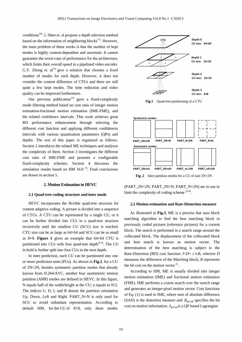
conditions10). L Shen et. al propose a depth selection method

based on the information of neighboring blocks11). However,

the main problem of these works is that the number of kept

modes is highly content-dependent and uncertain. It cannot

guarantee the worst-case of performance for the architecture,

which limits their overall speed in a pipelined video encoder.

G.Y. Zhong et. al12) give a solution that chooses a fixed

number of modes for each depth. However, it does not

consider the content difference of CTUs and there are still

quite a few kept modes. The time reduction and video

quality can be improved furthermore.

Our previous publication13) gave a fixed-complexity

mode filtering method based on cost ratio of integer motion

estimation-fractional motion estimation (IME-FME), and

the related confidence intervals. This work achieves great

RD performance enhancement through selecting the

different cost function and applying different confidences

intervals with various quantization parameters (QPs) and

depths. The rest of this paper is organized as follows.

Section 2 introduces the related ME techniques and analyzes

the complexity of them. Section 3 investigates the different

cost ratio of IME-FME and presents a configurable

fixed-complexity schemes. Section 4 discusses the

simulation results based on HM 16.0 5). Final conclusions

are drawn in section 5.

2. Motion Estimation in HEVC

2.1 Quad-tree coding structure and inter mode

HEVC incorporates the flexible quad-tree structure for

content adaptive coding. A picture is divided into a sequence

of CTUs. A CTU can be represented by a single CU, or it

can be further divided into CUs in a quad-tree structure

recursively until the smallest CU (SCU) size is reached.

CTU size can be as large as 64×64 and SCU can be as small

as 8×8. Figure 1 gives an example that 64×64 CTU is

partitioned into CUs with four quad-tree depth2)-4). The CU

in bold is further split into four CUs in the next depth.

In inter prediction, each CU can be partitioned into one

or more prediction units (PUs). As shown in Fig.2, for a CU

of 2N×2N, besides symmetric partition modes that already

known from H.264/AVC, another four asymmetric motion

partition (AMP) modes are defined in HEVC. In this figure,

N equals half of the width/height at the CU; n equals to N/2.

The indices U, D, L and R denote the partition orientation

Up, Down, Left and Right. PART_N×N is only used for

SCU to avoid redundant representation. According to

default HM, for the CU of 8×8, only three modes

(PART_2N×2N, PART_2N×N, PART_N×2N) are in use to

limit the complexity of coding scheme 2)-4).

2.2 Motion estimation and Rate-Distortion measure

As illustrated in Fig.3, ME is a process that uses block

matching algorithm to find the best matching block in

previously coded pictures (reference pictures) for a current

block. The search is performed in a search range around the

collocated block. The displacement of the collocated block

and best match is known as motion vector. The

determination of the best matching is subject to the

Rate-Distortion (RD) cost function J=D+λ×B, wherein D

measures the difference of the Matching block, B represents

the bit cost on the motion vector 3) .

According to HM, ME is usually divided into integer

motion estimation (IME) and fractional motion estimation

(FME). IME performs a coarse search over the search range

and generates an integer-pixel motion vector. Cost functions

of Eq. (1) is used in IME, where sum of absolute difference

(SAD) is the distortion measure and �� specifies the bit

cost on motion information.��is a QP based Lagrangian

Fig.1 Quad-tree partitioning of a CTU

Fig. 2 Inter partition modes for a CU of size 2N×2N

Depth 0

CU size：64×64

Depth 1

CU size：32×32

Depth 2

CU size：16×16

Depth 3

CU size：8×8

CTU

PART_2N×2N PART_2N×N PART_N×2N PART_N×N

PART_2N×nU PART_2N×nD PART_nL×2N PART_nR×2N

Symmetric modes

Asmmetric modes


59

Fig. 3 Motion estimation

multiplier for motion vector decision.

��,�� = �� + �� × �� (1)

FME performs a fine search in sub-pixel accuracy

around the integer motion vector derived in IME. In this

process, computation intensive interpolation filtering is

involved to generate the half-pixel and quarter-pixel samples.

Since the distortion costs among neighboring sub-pixel

samples are similar, higher accuracy is required for the

distortion computation for motion estimation. Cost function

of Eq. (2) is employed in FME. Hadamard transformed

difference (HAD) is the distortion measure, which is more

complex than SAD since it involves the transform of a block.

With the processes of transform and interpolation mentioned

above, FME has much higher computation complexity than

IME, especially when IME is greatly accelerated by the fast

search tools such as TZ search that implemented in HM 4).

��,�� = �� + �� × �� (2)

After the decision of fractional motion vector, partition

modes of each CU are evaluated, and the best mode is

selected. Then, the cost of the CU will be compared to the

cost sum of the four sub-CUs in the next depth for deciding

whether the further split is needed or not. More precise

decision is required to maximize the coding gain in the

mode decision and CU depth selection. Thus, sum of square

error (SSE) based cost function of Eq. (3) is used in these

processes. �mode is the Lagrangian multiplier for mode

decision. �mode represents bit cost of encoding the whole

block that includes the information of motion, mode and

residual. The calculation of �� needs intensive

computation since it involves (inverse) transform, (inverse)

quantization, reconstruction and entropy coding. These

procedures are highly dependent with each other and results

in high cost in real-time implementations. The ��

cost-based decision is also called full rate distortion

optimization (full RDO) 4), 5).

mode = �� + �mode× �mode (3)

Above all, different RD cost functions are employed in

different steps of ME. RD cost checks traversing on the

quad-tree structure and multiple prediction modes make ME

the most computational challenging part in HEVC encoding.

Motion search for IME part requires large external memory

access, which is a power consuming part in hardware design.

Literatures 14), 15) have proposed several efficient solutions

for the IME part and greatly reduced the external memory

bandwidth. Moreover, interpolation of FME also brings high

cost in hardware area which is discussed in the next section.

3. Proposed Fixed-Complexity FME Mode Filtering

FME is the major part in ME in terms of computation

expense on the processes of interpolation and RD cost

evaluation. Our simulation shows that even with only one

reference frame, the FME occupies more than 50% of the

encoding time. Therefore, low complexity FME algorithm is

critical for realizing fast encoding. Moreover, the

interpolation and the full RDO result in high hardware cost.

Reducing the operation times of interpolation and full RDO

can save a lot of cost on logical gates 14) 16). Our work

proposes a mode filtering algorithm to reduce the number of

modes to a fixed level for the FME part. This section firstly

introduces a two-loop ME structure and the incorporated

module of mode filtering. A new complexity measurement

is defined and how the proposed mode filtering module

effects on the FME complexity is explained. Then the

investigation on the cost ratio of IME-FME and a cost

ratio-based mode filtering algorithm is presented. Finally,

the configurable scheme is discussed.

3.1 Overview of the proposed mode filtering

In original HM, IME and FME for each CU are

performed sequentially in one loop, as illustrated in Fig. 4(a), the RD cost of all the partition modes are checked by IME

and FME in sequence. After that, inter mode with the

selected partition mode is compared with the modes of PCM,

intra and skip for the CU compress. When a CTU is

compressed with the one loop ME structure, the processing

of next CU will not be started until both IME and FME of

the current CU are all finished. In order to increase the

parallelism, the inter-dependency of IME and FME in one

CU are usually removed in real-time applications.

best

match

curren

block current picture reference picture

collocated

block

search

range


60

In this work, IME and FME in a CTU are departed into

two loops and the proposed mode filtering algorithm is

applied based on a two-loop ME structure, as illustrated in

Fig.4(b). The left part is the IME loop, in which all the

prediction modes for all the CUs across different depths are

checked by IME. The generated integer motion vectors and

IME costs for all CUs will be transmitted to the module of

mode filtering that selects a certain amount of modes for the

following FME loop. The integer motion vectors of the

selected modes are fed into the FME loop wherein the

fractional motion search and estimation are performed to

decide the best inter mode. With the two-loop ME structure,

FME for a CU will not be started before the IME for all the

CU in the same CTU are completed.

Since motion vectors are predicted from neighboring

blocks, separation of IME and FME inevitably leads to

inaccurate prediction of MVs. Our simulation shows that the

two-loop structure without mode filtering module increases

the BD rate by 0.09% and the encoding time by 3%

compared with one loop structure. The coding efficiency

loss is negligible. With the two-loop ME structure, the most

computationally intensive FME and the following mode

decision process is departed from IME. By applying

efficient mode filtering algorithm before FME, only a

limited number of modes with good IME costs will be

selected for the FME and full RDO. If the complexity of

FME can be reduced to a fixed level, it will benefit the

pipeline design for IME and FME.

In this paper, we introduce a new complexity

measurement for FME. Usually, execution time is used as

complexity measurement that is related to the content of the

processed picture, and other coding parameter like QP

values. However, for a CU with the same size, the number

of pixels that needs to be processed in the FME is the same.

In other words, the operation times related to hardware cost

are the same. Therefore, we introduce a more direct and

simple definition ‘layer’ to measure the complexity of FME.

The layer is proportional to the size of CU no matter what

partition mode they use. According to the HM with default

configuration, CTU is configured as 64×64 and four depths

are allowed. Seven modes can be selected for the CU in

depth 0, 1, 2 and three modes can be selected for the CU in

depth 3. We define the FME complexity of processing a

64×64 CU for one mode as 1 layer. If seven modes are

evaluated, the complexity of depth 0 is 7 layers. In depth 1,

the CU size is 32×32 and FME complexity is 1/4 layer for

one mode. Since there are 4 CPUs and seven modes in depth

1, the FME complexity of depth 1 is still 7 layers. It is easy

(a) One loop ME structure

(b) Two-loop ME structure with an inter mode filtering module

Fig. 4 One loop and two-loop ME structures

to find that the complexity of each depth is the same with

the allowed number of modes for this depth. Therefore, the

FME complexity for the whole CTU is 24(=7+7+7+3)

layers.

3.2 Proposed cost ratio-based mode filtering algorithm

The mode selection includes two aspects. One is mode

selection in the same depth. The other is mode selection

across different depths, which is called depth selection here.

In the latter case, a CU can be further split into 4 sub-CUs,

the RD cost of this CU in the upper depth is compared with

the cost sum of the four sub-CUs in the next depth in order

to decide whether the further split is necessary. If the depth

is selected, the corresponding mode of the CU in this depth

is necessary. Otherwise, the corresponding modes can be

omitted. In depth selection, since the number of partitions

increases a lot after being split into lower depth, the side

information of encoding motion vectors increases

significantly, especially for the case of low motion (since the

distortion is also small). Thus, it will lead to great error if the

IME cost is directly used for the depth selection. In order to

make better use of IME costs for the depth selection, the

relationship of IME cost and FME cost is investigated in the

next section. The FME cost here does not only refer to the cost of ��,�� that used in the fractional motion vector

decision but also the cost calculated based on the derived

fractional motion vector, such as ��. Similarly, IME cost

Compress a CU

Check RD Cost_Inter

IME

For all the modes

For all the CUs in a CTU

FME

PCM

Intra

Skip

IME-FME loop

Compress a CU

Check RD Cost_Inter

IME

Compress a CU

Inter mode

filtering

For all the modes

Check RD Cost_Inter

FME

For the remaining modes PCM

Intra

Skip

IME loop FME loop

For all the CUs in a CTU For all the CUs in a CTU


61

refers to the cost calculated based on the integer motion

vector.

3.2.1 Distribution of cost ratio and the related confidence interval

Figure5 depicts a scatter plot of IME cost and FME cost

for the sequence of BQSquare with QP equals to 22. The

horizontal axis �� refers to the cost of IME while the

vertical axis �� refers to the cost of FME. The cost ratio of

IME-FME is defined as Eq. (4) .

��/� = ��/�� (4)

In Fig.5, IME cost is ��,�� and FME cost is ��.

As shown in the figure, most of the points distribute in the area that clamped by line � and line �. The value of ��/� can be thought of being distributed within a range of ��, � . That is

� ! ��/� ! � . (5)

It implies that large IME cost does not necessarily

results in large FME cost. That is why the IME costs are not

used directly for the mode decision for all the cases. Supposing the cost ratio of ��/� confirms to normal

distribution, ��, � can be regarded as a confidence interval

(CI) that constructed with a given confidence level. By fitting a probability distribution to the sample data of ��/� with MATLAB, normal distribution of ��/� with two

parameters " (mean value) and# (standard deviation) can

be created. If we choose a confidence level $ ∈ &0,1), the

upper limit and lower limit of the confidence interval can be

calculated as " * +,/- . /√12, where the critical value +,/-

can be derived by checking the Z-table17). Giving different

confidence levels, different confidence intervals can be

derived.

Fig. 5 IME cost and FME cost for the sequence of BQSquare

Figure 6 gives the probability density function (PDF) of the ��/� related to ��,�� and ��. It is obvious that

there are some bias and the function is not completely fit

with the normal distribution. From our investigation, we find

that the cost ratio can generally follow the normal

distribution if the cost functions of the IME and FME are

carefully selected. As shown in Fig.7, if the SAD is used as IME cost and HAD is used as FME cost, the PDF of ��/� fits well with normal distribution. According to the

distribution of cost ratio, it is possible to estimate the

confidence interval of FME cost with the IME cost.

3.2.2 Confidence interval-based mode filtering (CI-MF)

Our simulation shows that the confidence interval varies

with QP and depth for a given confidence level.

If the cost ratio and related confidence interval of depth

n is represented as Eq. (6),

�1 ! �&�/�)3 = 453463

! �1, (6)

for different depth 7 and 8, we get

�9 ! �&�/�): = 45:46:

! �9 ,

(7)

�; ! �&�/�)< = 45<46<

! �; .

(8)

If the following condition of Eq. (9) is satisfied,

�;��< =�9��: (that is 46:46<

> ?@A:

)

(9)

we can get

��: > ��< .

(10)

Fig. 6 PDF of cost ratio of ��,�� -�� for the sequence

of BQSquare


62

Fig.7 PDF of cost ratio of SAD-HAD for the sequence of

BQSquare

If depth k is the upper depth, this conclusion means that

FME cost of the CU in depth k is lar ger than the cost sum of

the corresponding sub-CUs in depth j. In other words, depth

k should have lower priority and is more likely to be

removed for this CU. From the above derivation, we find

that the depth selection is realized by comparing the IME

cost ratio to a parameter that is related to the confidence

intervals. The parameter is called mode filtering parameter

(MFP) and this depth selection method is called confidence

interval-based mode filtering (CI-MF). The related

confidence intervals can be derived from training based on

the distribution of cost ratio from the statistics.

Since there are up to seven modes in one depth, it is

complex to compare each mode in the current depth to the

other mode combinations in the lower depth. In order to

simplify the comparison, some unlikely modes are firstly

removed for each depth. Then the depth selection is

performed among the kept modes. For the same depth, since

each mode includes one or two partitions, bit cost of all the

modes are in the same level. Thus, the SAD-based IME cost

is directly used for the mode selection in the same depth. To

avoid large performance loss, two modes with the smallest

IME costs are kept.

For the depth selection, the previous work13) uses the

cost ratio of ��,�� -�� which is in accord with the

original HM. This work employs the cost ratio of

SAD-HAD for the following three reasons. Firstly, the

confidence interval is derived from the statistic of cost ratio ��/�. Based on the assumption that the cost ratio conforms

to the normal distribution, cost ratio of SAD-HAD is much

better in terms of the conformity with normal distribution.

Secondly, since depths are checked from upper to lower,

modes in the upper depth that meet certain conditions will

be selected firstly, which gives higher priority to the upper

depth. It can be taken as a complement of removing the part

of bit cost from the cost function. Thirdly, it is very common

that HAD or HAD based cost are directly used as the

measurement of mode decision, since the calculation of

�� is complex and relatively hard to be implemented in

real application18)-20).

The other problem is how to reduce the complexity to a

fixed level. The complexity of a CU in terms of layers is

proportional to size and allowed number of modes of this

CU. For each CTU, there are up to 85 CUs with 339 modes

needs to be checked in some order. It is difficult to control

the whole complexity of a CTU in a fixed level if the

number of kept modes for each CU is different and random.

This work keeps the same number of modes for the CUs in

the same depth. CUs in the depth with higher priority will be

assigned more modes. The complexity of each depth in

terms layers is equals to the allowed number of modes, and

the whole complexity of a CTU equals to the sum of the

allowed numbers for all the depths. By adjusting the allowed

number of modes for each depth, the whole complexity of

the CTU can be controlled easily.

Figure 8 depicts the process of CI-MF for one depth.

Cost of the current depth is compared with that of other

lower depths to evaluate their priorities. For depth 0, the

lower depths are depth 1, 2 and 3. Cost of a depth is defined

as the cost sum of all the CUs in this depth. As mentioned

previously, before depth selection, the best two modes with

smaller IME cost are kept for each CU. Therefore, the cost

of a depth has a range with a minimum and a maximum

value. For depth 0, there is only one CU, thus the minimum

and maximum cost of this depth are the cost of the best

mode and the second-best mode of the CU, respectively. In

the flow chat of Fig.8, depth n is the current depth needs to

be processed. For depth n, the minimum cost and maximum

cost are marked as �1B and �1C. �1B equals the cost sum

of the best modes for all the CUs in this depth and �1C

equals the cost sum of all the second-best modes. Two cost

values of the current depth are compared to the average cost

of other lower depths respectively to decide how many

modes are kept for this depth. �1D�E�� is used to represent

the average cost of the lower depths, which is calculated as

Eq. (11). �1D�E�� is the average upper limit of CIs of other

lower depths which is calculated as Eq. (12). FGH1 is the

mode filtering parameter that related to CI. It is defined in

Eq. (13), where �1 is the lower limit of CI for depth n. All

the parameters mentioned above are not used for depth 3 (n


63

should not be 3), since the allowed number of modes of the

last depth can be calculated directly when the upper depths

are all processed.

�1D�E�� = 1&3 − K) L �MB +�MC

2 ,O

MP1QC&0 ! K ! 2)

(11)

�1D�E�� = 1∑ 4MOMP1QC

L 4M�M ,O

MP1QC&0 ! K ! 2)

(12)

FGH1 = �1D�E��1

, &0 ! K ! 2) (13)

F1 in the flow chart is used to record the number of

kept modes and it is initialized to 0. For the complexity

control of the whole CTU, F1 should be limited in a range

of �T1 , U1 , where T1 is the lower limit and U1 is the

upper limit for depth K. The limits are decided by the

number of modes that have been kept for the upper depths

and the expected complexity of the whole CTU. They are

updated instantly with the progress of mode filtering. If

T1 = U1, as shown in Fig.8, the number of modes need to

be kept is fixed and the following evaluation is unnecessary.

For example, there is no mode for depth 0 and 1 that is kept

in the previous process, but the expected complexity is 4. In

this case, for depth 2 and depth 3, both T1 and U1 are

equal to 2. F1 is also equal to 2.

For the normal case that U1 is larger than T1, F1 is

derived by comparing the two cost ratios of �1B/�1D�E��

and �1C/�1D�E�� to the mode filtering parameter FGH1.

Then, F1 is adjusted based on the limits of T1and U1 .

�1B is smaller than �1C and the comparison starts with

�1B/�1D�E��. The progress mainly includes the following

three cases.

(1) If �1B/�1D�E�� is larger than FGH1, depth n with the best mode has no priority compared to other lower depths. The best mode in depth n is removed in the mode filtering. In this case, the second-best mode should also be removed and F1 equals to 0. If T1 > 0, it means that the kept modes are not enough for keeping the whole complexity in a fixed level. Although both modes are not good enough, one or two modes should be remained. In this case, F1is set to T1, (F1 = T1).

(2) If the ratio of �1B/�1D�E�� is equal or smaller than FGH1, It implies that the best mode in depth n is better than modes in other lower depths. The best

Fig. 8 CI-MF for one depth

mode should be kept for depth n. Thus, F1 is updated to 1. Then, �1C/�1D�E�� will be checked and the process goes to the case (3).

(3) If �1C/�1D�E�� is larger than FGH1, the second-best

mode should be removed, F1 is still equal to 1 and

finally determined. If �1C/�1D�E�� is smaller or equal

than FGH1the second-best mode should be kept and

F1 is updated to 2.In this case, the maximum number

of allowed modes for this depth should be checked. If

F1 > U1, the final value of F1 should be adjusted to

U1 (F1 = U1).

By applying the same process for each depth, the kept

modes across all the depths are decided. The FME will be

performed to the kept modes.

3. 3 Proposed configurable CI- MF with k layers (CI- MF-k)

For a CTU, layers of FME equals to the sum of numbers

of kept modes for all the depths. As described in previous

section, CI-MF generates the number of kept modes F1

for each depth. It is related to the number of modes that have

been decided as far and the expected complexity on FME.

Figure 9 describes the configurable scheme, wherein k

Mn=0;

[Ln , Un];

(the given values)

Ln=Un

Mn=0 Cn0/CnLower > MFPn

Mn=1

Ln > 0

Mn=Ln

Cn1/CnLower > MFPn

Mn=2

Store Mn;

Calculte [L(n+1) , U(n +1)];

Step to depth (n+1)

N

Y

Y

N

N

Y

N

Y

Mn> Un Mn=Un

Y

N


64

Fig.9 Configurable CI-MF-k scheme

represents layers of FME for each CTU that should be fixed

by applying CI-MF. The range of F1 changes with

different value of k. Accordingly, F1 may be different. By

using this method, the complexity of the FME can be

adjustable for different encoding requirement.

4. Simulation Results and Analysis

Simulation is implemented in HM 16.0 with the test

configuration of Low-Delay-P (LDP) main 21). Since one

reference frame scheme is quite common in real-time

application, only one reference frame is employed in this

simulation. Other coding parameters are exactly accord with

the default configuration recommended by JCT-VC.

Simulation includes confidence intervals training and

performance evaluation of CI-MF. The confidence intervals

for different QPs and depths are obtained by training. As

listed in Table 1, 21 Sequences from Class A to Class E that

are recommended by JCT-VC are tested in the simulation.

In the training, 3 sequences are randomly selected from each

class, and 15 sequences are employed.

Firstly, the samples of cost ratio are taken from the

training sequences. Based on the statistic computation with

MATLAB, the mean value and standard deviations for

different QPs and depths are derived. Then, for the training

sequences, the confidence level is set from 50% to 95% with

a step of 5%. The confidence intervals with the smallest

average BD rate for the training sequences are selected and

implemented in the CI-MF algorithm. Four training sessions

with different training sequences are used to verify the

reliability of the training method. In our experiments, it is

found that the trained confidence intervals and the

corresponding BD rate results of the four sessions are close

with each other.

Therefore, it is possible to get reliable confidence

intervals with the proposed training method. The confidence

intervals derived from one of the training sessions are used

for the final simulation. The sequences of this training

session are listed in the second row of Table 1. Table 2 shows confidence intervals from the training.

Cases 1, 2, 3 in Table 1 are executed with the proposed

configurable CI-MF-k with k equals to 4, 5 and 6

respectively. They are all compared to the anchor of original

HM to evaluate the efficiency of the proposed CI-MF

algorithm. Moreover, the three cases are compared with

each other to show how the RD performance and encoding

time change with the different FME complexity setting.

Since this work is focused on reducing the complexity of

FME part, the FME complexity is firstly measured by a

parameter of layers for each CTU. This measurement is

related to the complexity in terms of hardware cost since it is

related to the number of pixels needs to be processed in the

FME. By keeping the same number of modes for CUs with

the same size and limiting the total number of modes across

four depths, CI-MF-k fixes the complexity of FME in k

layers for each CTU. The result is fixed regardless of video

content and some encoding parameters like QP. HM has

Give kCalculate [Ln , Un]

based on k and stored Mi ( i<n )

Perform CI-MF;

store Mn

For depth n

Table 1 Experiment Condition

Sequences

for

simulation

21 Sequences from Class A～E;

Class A (2560×1600): Traffic, PeopleOnStreet, Nebuta,

SteamLocomotive;

Class B (1920×1080): Kimono, ParkScene, Cactus,

BasketballDrive, BQTerrace;

Class C (832×480): BasketballDrill, BQMall,

PartyScene, RaceHorsesC

Class D (416×240): BasketballPass, BQSquare,

BlowingBubbles, RaceHorses

Class E (1280×720): Johnny, Vidyo1, Vidyo3, Vidyo4

Training

sequences

(Resolution)

15 sequences; 3 sequences from each class.

Class A: Traffic, Nebuta, SteamLocomotive;

Class B: Cactus, BasketballDrive, BQTerrace;

Class C: BasketballDrill, BQMall, PartyScene;

Class D: BasketballPass, BlowingBubbles, RaceHorses;

Class E: Vidyo1, Vidyo3, Vidyo4.

Max CU/depth

64/4

GOP structure

LDP configuration (IPPP, reference frame number:1)

QP 22, 27, 32, 37

Comparison

cases

Anchor: Original HM;

Case1: HM with CI-MF-4;

Case2: HM with CI-MF-5;

Case3: HM with CI-MF-6.

Table 2 Confidence intervals from training

an/bn /QP 22 27 32 37

a0 1.7158 1.6987 1.6654 1.6092

b0 1.7822 1.7592 1.7206 1.6611

a1 1.7405 1.7227 1.6871 1.6272

b1 1.8136 1.7896 1.7493 1.6880

a2 1.7637 1.7432 1.7052 1.6437

b2 1.8374 1.8112 1.7701 1.7090

a3 1.7565 1.7402 1.7062 1.6524

b3 1.8331 1.8146 1.7809 1.7298


65

incorporated many fast mode decision tools such as ESD

(early skip detection), CFM (coding block flag based fast

mode) and ECU (early CU termination) 22). By enabling

these tools, some CU or PU modes will be skipped, but the

layers for each CTU will not be fixed. All the fast tools are

disabled in default in HM. Our simulation employs the

default setting that all the CU and PU modes should be

traversed and the FME complexity is 24 layers for each

CTU. FME complexity results in terms of layers for each

CTU is shown in Fig. 10.

The performance of the proposed work is compared to

the original HM and the result is listed in Table 3. WXYZ[

and WX[1\ are FME time reduction and encoding time

reduction of the proposed work compared to Original HM,

which are calculated as Eq. (14) and Eq. (15).

XYZ[&]^_`_K�a) and XYZ[&b^]b]cde) represent FME

time for the original HM and the proposed work,

respectively. X[1\&]^_`_K�a) and X[1\&b^]b]cde) represent the encoding time for the original HM and the

proposed work, respectively. RD performance of the

proposed algorithm is measured by the Bjøntegaard-Delta

rate (BD rate), which is calculated based on the results of

PSNR and bitrate with four QPs. It corresponds to the

average bitrate difference in percent for the same PSNR 23).

WXYZ[ = XYZ[&]^_`_K�a) − XYZ[&b^]b]cde)XYZ[&]^_`_K�a) (14)

WX[1\ = X[1\&]^_`_K�a) − X[1\&b^]b]cde)X[1\&]^_`_K�a) (15)

For the same sequence, WXYZ[ with different QP

values is close since the reduced number of layers is the

same. While the WX[1\ increases as QP value increases. In

the following paper, we only discuss the average result

across different QP values. Taking the proposed HM with

CI-MF-6 for an example, we discuss how the proposal

effects the complexity and BD rate. By keeping only 6

modes across 4 depths, the FME complexity is reduced from

24 layers to 6 layers. FME is accelerated by 72.70% as

expected. The whole encoding is accelerated by 44.22% as

well. The proposed algorithm works better for the sequences

with larger size. For example, the BD rate loss is even less

than 0.1% for some sequences like SteamLocomotive from

Class A.

However, for sequences from Class D with small size,

the BD rate loss is significant. It is because that CTUs in the

pictures with small size contains much more details

compared to those in large size. Therefore, keeping the same

number of modes for all the CUs in the same depth and

reducing the number of modes to a low value bring much

more loss for these videos. Comparing the results of the

three cases, it is obvious that for each reduced one layer (k

reduced by 1), WXYZ[ increases by 5% while the WX[1\

increases by 3%. When only 4 layers are kept, the FME time

and encoding time reduction are up to 82.75% and 49.42%

respectively. The BD rate loss is 1.63% on average. When

the FME complexity is set from 4 to 6, the BD rate shows

large improvement. We can set the complexity of the FME

to different level for different encoding requirement.

The performance comparison between original HM and

HM with CI-MF-4 for six sequences from different class is

also shown in Fig. 11 by RD curves. The RD curve in black

represents the performance of original HM while the curve

in red represents the performance of HM with CI-MF-4. The

high conformity of two RD curves means that the

performance of the two cases is quite close, such as the

curves of the sequence of SteamLocomotive, as shown in

Fig.11(b). For the sequence of BQSquare, the curve of

CI-MF-4 is obviously below the curve of original HM,

which means that the performance of CI-MF-4 is decreased

compared the original HM, as shown in Fig.11(e). Our result

shows that the BD rate of BQSquare is increased by 3.25%

(PSNR loss 0.085dB and the bitrate increases 1.21% on

average.)

The subjective visual quality comparison between

original HM and HM with CI-MF-4 for the sequence of

Kimono that has obvious texture and high motions are

displayed. The reconstructed pictures with two QP values

(22, 32) for the sixth frame are shown in Fig. 12. A 960×540

window is zoomed out from the frame of 1920×1080 size to

show the details. Fig. 12(a) and Fig. 12(b) are the pictures

encoded with QP of 22; Fig. 12(c) and Fig. 12(d) are the

Fig.10 Complexity of FME

FME complexity (# layers/CTU)

0 4 8 12 16 20 24

Original HM

HM with CI-MF-6

HM with CI-MF-5

HM with CI-MF-4

24

6

5

4


66

pictures encoded with QP of 32. With the proposed

CI-MF-4, PSNR is decreased by 0.03dB and 0.14dB for the

QP of 22 and 32 respectively compared to original HM. But

the quality difference cannot be captured by human eyes. In

other words, the proposal has almost the same subjective

quality with the original HM.

Table 4 shows the comparison results between CI-MF-4

and the previous work13). The results of CI-MF-4 in this

table are corresponding to the result that listed in Table 3. In

the performance comparison, we firstly implemented the

previous method with HM16.0 that we used for this work.

Secondly, we performed the simulation with the same

environment and conditions. Both previous work and our

proposal reduce FME from 24 layers to 4 layers. They

achieved 84.56% and 82.75% FME time reduction,

respectively. But improving the cost function and applying

the adaptive CI according to different QP and depth, the

performance of this work is much better. The BD rate loss is

reduced from 2.18% to 1.63% on average.

5. Conclusion

In this paper, we present a low-complexity FME mode

filtering algorithm CI-MF. It utilizes the ratio of IME-FME

and the related confidence intervals to select the modes for

different depths and keep the complexity of FME to a fixed

level. The proposed CI-MF can be configurable for different

encoding time and RD performance requirements.

Table3 Performance comparison of HM with CI-MF-4, CI-MF-5, CI-MF-6, with original HM

Class Sequence HM with CI-MF-4 HM with CI-MF-5 HM with CI-MF-6

BD rate [%]

∆XYZ[

∆X[1\

BD rate [%]

∆XYZ[

∆X[1\

BD rate [%]

∆XYZ[

∆X[1\

A

Traffic 1.53% 83.46% 52.40% 0.91% 78.06% 49.44% 0.82% 72.65% 46.30%

PeopleOnStreet 1.27% 77.70% 42.52% 1.00% 73.38% 40.84% 0.98% 68.92% 38.60%

Nebuta 1.28% 79.10% 39.70% 0.88% 74.39% 37.82% 0.38% 69.69% 35.65%

SteamLocomotive 0.06% 85.83% 51.19% 0.01% 80.16% 48.30% 0.00% 74.27% 45.09%

Average 1.03% 81.52% 46.45% 0.70% 76.50% 44.10% 0.55% 71.38% 41.41%

B

Kimono 3.12% 78.00% 44.66% 1.56% 73.46% 42.64% 1.24% 69.06% 39.82%

ParkScene 1.40% 84.08% 52.33% 0.80% 78.39% 49.44% 0.74% 73.32% 46.61%

Cactus 1.62% 83.62% 50.79% 1.08% 78.67% 48.21% 1.16% 73.35% 45.40%

BasketballDrive 2.17% 82.85% 49.32% 1.36% 77.79% 46.97% 1.19% 72.74% 44.33%

BQTerrace 1.34% 84.52% 51.30% 0.85% 79.07% 48.58% 0.73% 73.48% 45.57%

Average 1.93% 82.62% 49.68% 1.13% 77.48% 47.17% 1.01% 72.39% 44.35%

C

BasketballDrill 1.77% 82.38% 48.81% 1.21% 78.80% 46.59% 1.01% 73.11% 43.90%

BQMall 1.39% 83.67% 50.95% 0.80% 78.77% 48.22% 0.82% 73.30% 45.64%

PartyScene 1.09% 82.58% 45.10% 0.73% 78.03% 43.03% 0.66% 72.56% 40.42%

RaceHorsesC 1.95% 78.48% 40.06% 1.37% 74.17% 38.70% 1.00% 68.85% 36.56%

Average 1.55% 81.78% 46.23% 1.03% 77.45% 44.14% 0.87% 71.96% 41.63%

D

BasketballPass 1.45% 82.88% 50.92% 1.30% 77.46% 48.83% 0.66% 74.14% 46.63%

BQSquare 3.25% 85.85% 48.66% 1.95% 81.45% 46.47% 1.88% 75.07% 42.71%

BlowingBubbles 2.41% 80.53% 46.04% 1.57% 76.77% 43.12% 1.40% 73.23% 42.26%

RaceHorses 1.82% 77.91% 39.47% 1.68% 74.36% 37.55% 1.44% 71.57% 36.64%

Average 2.23% 81.79% 46.27% 1.63% 77.51% 43.99% 1.35% 73.50% 42.06%

E

Johnny 1.43% 86.14% 59.31% 1.59% 80.21% 55.99% 0.74% 74.72% 52.44%

Vidyo1 0.93% 86.22% 58.91% 0.61% 80.35% 55.62% 0.53% 74.37% 52.16%

Vidyo3 1.90% 85.62% 56.73% 1.29% 79.62% 53.72% 0.90% 73.74% 50.18%

Vidyo4 1.09% 86.30% 58.73% 0.57% 80.28% 55.30% 0.44% 74.53% 51.73%

Average 1.34% 86.07% 58.42% 1.02% 80.12% 55.16% 0.65% 74.34% 51.63%

Average for all 1.63% 82.75% 49.42% 1.10% 77.79% 46.92% 0.89% 72.70% 44.22%


67

Simulation results demonstrate that the proposed

CI-MF-4 scheme achieves 82.75% FME time reduction with

1.63% BD rate increasement compared to the original HM

with full FME. The proposed algorithm is friendly to the

hardware design. It will be applied to the ME part to solve

the complexity problem in the real-time application in the

future.

Acknowledgement

This work is supported by JST, PRESTO Grant Number

JPMJPR1757 Japan.

(a) Nebuta (b) SteamLocomotive

(c) BQTerrace (d) PartyScene

(e)BQSquare (f) Vidyo3

Fig. 11 RD curves for different sequences


68

References

1) Recommendation ITU-T H.264 | International Standard ISO/IEC

14496-10: “Advanced video coding for generic audiovisual services’’

(2019).

2) Recommendation ITU-T H.265 | International Standard ISO/IEC

23008-2: “High efficiency video coding’’ (2019).

3) M. Wien, High Efficiency Video Coding : Coding tools and

Specification, Springer, pp.179-202 (2014).

4) K. McCann, C. Rosewarne, B. Bross, M. Naccari, K. Sharman, G.

Sullivan: “High Efficiency Video Coding (HEVC) Test Model 16

(HM 16) Improved Encoder Description”, 19th meeting of Joint

Collaborative Team on Video Coding (JCTVC), document

JCTVC-W14970, Strasbourg (2014).

5) Joint Collaborative Team on Video Coding, HEVC Reference

Software, HM16.0,

https://hevc.hhi.fraunhofer.de/svn/svn_HEVCSoftware/tags/.

6) Y.-J. Wang, C.-C. Cheng, T.-S. Chang: “A Fast Algorithm and Its

VLSI Architecture for Fractional Motion Estimation for

H.264/MPEG-4 AVC Video Coding”, IEEE Trans. on Circuits and

Systems for Video Technology Vol.17, No.5, pp.578-583 (2007).

7) T.-Y. Kuo, Y.-K. Lin, T.-S. Chang: “SIFME: A Single Iteration

Fractional-Pel Motion Estimation Algorithm and Architecture for

HDTV Sized H.264 Video Coding”, Proc. of International

Conference on Acoustics, Speech and Signal (ICASSP), pp.1185 –

1188 (2007).

8) P.-K. Tsung, W.-Y. Chen, L.-F. Ding, C.-Y. Tsai, T.-D. Chuang, L.-G.

Chen: “Single-Iteration Full-Search Fractional Motion Estimation for

Quad Full HD H.264/AVC encoding”, Proc. of IEEE International

Conference on Multimedia and Expo (ICME), pp. 9-12 (2009).

9) J. Kim, J. Yang, K. Won, B. Jeon: “Early Determination of Mode

Decision for HEVC”, Proc. of Picture Coding Symposium (PCS), pp.

449-453 (2012).

10) Q. Yu, X. Zhang, S. Wang, S. Ma: “Early Termination of Coding Unit

(a) Kimono coded by original HM (QP: 22; PSNR: 41.6213dB) (b) Kimono coded by HM with CI-MF-4 (QP: 22; PSNR: 41.5920dB)

(c) Kimono coded by original HM (QP: 32; PSNR: 36.7252dB) (d) Kimono coded by HM with CI-MF-4 (QP: 32; PSNR: 36.5869dB)

Table 4 Performance comparison with previous work

Seq. Class Previous work13) CI-MF-4

BD rate [%] ∆XYZ[ ∆X[1\ BD rate [%] ∆XYZ[ ∆X[1\

A 1.08% 83.95% 47.48% 1.03% 81.52% 46.45%

B 2.22% 84.87% 50.68% 1.93% 82.62% 49.68%

C 2.00% 83.25% 46.95% 1.55% 81.78% 46.23%

D 3.92% 83.42% 46.92% 2.23% 81.79% 46.27%

E 1.67% 87.24% 59.09% 1.34% 86.07% 58.42%

Ave. 2.18% 84.56% 50.25% 1.63% 82.75% 49.42%


69

Splitting for HEVC”, Proc. of Asia Pacific Signal and Information

Processing Association Annual Summit and Conference (APSIPA),

pp. 1-4 (2012).

11) L. Shen, Z. Liu, X. Zhang, W. Zhao, Z. Zhang: “An Efficient CU Size

Decision Method for HEVC Encoders”, IEEE Trans. on Multimedia,

Vol. 15, No. 2, pp. 465-470 (2013).

12) G.-Y. Zhong, X.-H. He, L.-B. Qing, Y. Li: “Fast Inter-Mode Decision

Algorithm for High-Efficiency Video Coding Based on Similarity of

Coding Unit Segmentation and Partition Mode between Two

Temporally Adjacent Frames”, Journal of Electronic Imaging, Vol. 22,

No. 2, pp. 381-388 (2013).

13) J. Zhou, Y. Zhou, D. Zhou, S. Goto: “A fixed-complexity HEVC Inter

Mode Filtering Algorithm Based on Distribution of IME-FME Cost

Ratio”, IEEE International Symposium on Circuits and Systems

(ISCAS), pp. 617-620 (2015).

14) M. E. Sinangil, V. Sze, M. Zhou, A. P. Chandrakasan: “Cost and

Coding Efficient Motion Estimation Design Considerations for High

Efficiency Video Coding (HEVC) Standard”, IEEE Journal of

Selected Topics in Signal Processing, Vol. 7, No. 6, pp. 1017-1028

(2013).

15) D. Zhou, J. Zhou, G. He, S. Goto: “A 1.59Gpixel/s Motion

Estimation Processor with -211-to-211 Search Range for UHDTV

Video Encoder”, IEEE Journal of Solid-State Circuits (JSSC), Vol. 49,

No. 4, pp. 827-837 (2014).

16) V. Sze, M. Budagavi，G. J. Sullivan: “High Efficiency Video Coding

(HEVC): Algorithms and Architectures”, Springer, pp.303-341

(2014).

17) Wikipedia, “Standard normal table”, https://en.wikipedia.org/wiki/

Standard_normal_table/.

18) X. Zhao, J. Sun, S. Ma, W. Gao, “Novel Statistical Modeling,

Analysis and Implementation of Rate-Distortion Estimation for

H.264/AVC Coders”, IEEE Trans. on Circuits and Systems for Video

Technology, Vol. 20, No. 5, pp. 647-660 (2010).

19) Y-K. Tu, J-F. Yang, M-T. S, “Efficient Rate-Distortion Estimation for

H.264/AVC”, IEEE Trans. on Circuits and Systems for Video

Technology, Vol. 16, No. 5, pp. 600-611 (2006).

20) Q. Wang, D. Zhao, W. Gao, S. Ma, “Low Complexity RDO Mode

Decision Based on a Fast Coding-Bits Estimation Model for

H.264/AVC”, Proc. of IEEE International Symposium on Circuits

and Systems (ISCAS), pp. 3467-3470 (2005).

21) F. Bossen: “Common Test Conditions and Software Reference

Configurations”, 11th meeting of Joint Collaborative Team on Video

Coding (JCTVC), document JCTVC-K1100, Shanghai, China

(2012).

22) K.-M. Lin, J.-R. Lin, M.-J. Chen, C.-H. Yeh, C.-A. Lee: “Fast

Inter-prediction Algorithm Based on Motion Vector Information for

High Efficiency Video Coding”, Journal on Image and Video

Processing, Vol. 99, pp. 1-17 (2018).

23) G. Bjøntegaard: “Calculation of Average PSNR Differences between

RD-Curves”, 13th meeting of Video Coding Experts Group, document

VCEG-M33, Austin, Texas, USA (2001).

（Received March 20, 2019）

（Revised January. 27, 2020）

Muchen LI

She received the B.S degrees from the Physics Department of the East China Normal University, Shanghai, China in 2006, and the M. E degree from Waseda University, Kitakyushu, Japan, in 2011. She completes the doctor courses in Waseda University in 2017. She is currently a researcher in Hosei University, Tokyo, Japan. Her research interests include algorithms and VLSI architectures for multimedia processing and compressive sensing.

Jinjia ZHOU (Member)

She received the B.E. degree from Shanghai Jiao Tong University, Shanghai, China, in 2007, and the M.E. and Ph.D. degrees from Waseda University, Kitakyushu, Japan, in 2010 and 2013, respectively. She was a Researcher with Waseda University from 2013 to 2016. She is currently an Associate Professor with Hosei University, Tokyo, Japan. She is also a JST researcher, Tokyo, Japan，

and She is also a senior visiting scholar in State Key Laboratory of ASIC & System, Fudan University, China. Her current research interests include algorithms and VLSI architectures for multimedia processing and artificial intelligence.. Dr. Zhou is a recipient of the Chinese Government Award for Outstanding Student dents Abroad of 2012. She received the Hibikino Best Thesis Award in 2011. She was a co-recipient of ISSCC 2016 Takuo Sugano Award for Outstanding Far-East Paper, the best student paper award of VLSI Circuits Symposium 2010 and the design contest award of ACM ISLPED 2010. She participated in the design of the world first 8K UHDTV video decoder chip, which was granted the 2012 Semiconductor of the Year Award of Japan. She works as a reviewer for journals including IEEE Trans. Circuits Syst. Video Tech., IEEE Trans. Circuits Syst. I, IEEE Trans. VLSI Syst., and IEEE Trans. Multimedia and so on.

Sotoshi GOTO

He received the B.E. and the M.E. Degrees in Electronics and Communication Engineering from Waseda University in 1968 and 1970 respectively. He also received the Dr. of Engineering from the same University in 1978. He joined NEC Laboratories in 1970 where he worked for LSI design, Multimedia system and Software as GM and Vice President. Since 2002, he has been Professor, at Graduate school of Information, Production and Systems of Waseda University at Kitakyushu. He served as GC of ICCAD, ASPDAC, VLSI-SOC, ASICON and ISOCC and was a board member of IEEE CAS society. He is IEEE Life Fellow and IEICE Fellow. He is Visiting Professor at Shanghai Jiao Tang University and Tsinghua University of China and Member of Science Council of Japan.


70

Call for Papers

Special Issue on Image-Related Technologies for the Realization of Future Society

IIEEJ Editorial Committee

There is a great expectation for an advanced and comfortable society brought about by economic development

and the solution of social issues through the introduction and spread of ICT technology. For this expectation, the

government advocates and promotes Society 5.0 as a new future society, following hunting society (Society 1.0),

agricultural society (Society 2.0), industrial society (Society 3.0), and information society (Society 4.0). It is

clearly stated that this purpose is to build a system that coalesces cyber space (virtual space) and physical space

(real space) at a high level, and integrates drones, AI devices, medical / nursing care, smart work, smart

management and autonomous driving etc.

Not only image recognition and visualization, but also XR that integrates virtual reality (VR), augmented reality

(AR), mixed reality (MR) is also necessary to make cyber space more familiar. In addition to visual effects,

cross-modal sensory presentation that appeals to the human senses is emphasized. Therefore, technological

innovation in computer graphics, computer vision, user interface, user experience, etc., which form these

technological foundations, is important, and practical application of technology that appeals not only to vision but

also to other senses through images and video.

In this special issue, we look forward to receiving your papers, system development papers, and data papers that

will realize a future society through images and video.

1. Topics covered include but not limited to

VR, AR, MR, Computer graphics, Image processing, Interaction, Realtime processing, Cross-modal sensory,

Computer vision, Machine learning Image analysis, Object detection, Image recognition, User interface, User

experience

2. Treatment of papers

Submission paper style format and double-blind peer review process are the same as an ordinary contributed

paper. If the number of accepted papers is less than the minimum number for the special issue, the acceptance

paper will be published as an ordinary contributed paper. We ask for your understanding and cooperation.

3. Publication of Special Issue:

IEEJ Transactions on Image Electronics and Visual Computing Vo.9, No.1 (June 2021)

4. Submission Deadline

Friday, October 30, 2020

5. Contact details for Inquires:

IIEEJ Office E-mail: [email protected]

6. Online Submission URL: http://www.editorialmanager.com/iieej/

71

ITUKALEIDOSCOPE2020

12TH ITU ACADEMIC CONFERENCE

Industry-driven digital transformation

CALL FOR PAPERS

7-11 DecemberONLINE

Organized bySupported byTechnically co-sponsored by

72

ThemeThe Fourth Industrial Revolution has data analytics at its core, and relies on innovations in fields such as robotics, cyber-physical systems, digital twins, virtual simulation, augmented reality, edge computing, artificial intelligence and blockchain – innovations all contributing to digital transformation of industrial processes.

In particular, the manufacturing sector has been an early adopter of new technologies capitalizing on connectivity and intelligence, but these technologies introduce endless possibilities – the automotive, energy, retail and healthcare industries are all moving in this direction.

ObjectiveKaleidoscope 2020 calls for original academic papers sharing insight into ongoing projects and research relevant to digital transformation. It targets specialists in the fields of ICT and socio-economic development, including researchers, academics, students, engineers, policymakers, regulators, innovators, and futurists.

Date and venueDue to COVID-19, Kaleidoscope 2020 will be held exceptionally online from 7-11 December 2020.

Submission of papersProspective authors are invited to submit full, original papers. The submission should be within eight pages, including a summary and references, using the template available on the conference’s website. All papers will go through a double-blind peer-review process. Submission must be made electronically; see http://itu.int/go/K-2020 for more details on online submission (EDAS). Paper proposals will be evaluated based on content, originality, clarity, relevance to the conference’s theme and, in particular, significance to future standards.

Deadlines extended

Submission of full paper proposals: 29 June 2020

Notification of paper acceptance: 25 September 2020

Submission of camera-ready accepted papers: 16 October 2020

Publication and presentationAccepted and presented papers will be published in the Conference Proceedings and will be submitted for inclusion in the IEEE Xplore Digital Library. The best papers will also be evaluated for potential publication in the IEEE Communications Standards Magazine. In addition, extended versions of selected papers will be considered for publication in the International Journal of Technology Marketing, the International Journal of Standardization Research, or the Journal of ICT Standardization.

AwardsA prize fund totalling CHF 6 000.- will be shared among the authors of the three best papers, as judged by the Steering and Technical Programme Committees. In addition, young authors of up to 30 years of age presenting accepted papers will receive Young Author Recognition certificates.

KeywordsInformation and communication technologies (ICTs), standards, digital transformation, manufacturing and energy management, smart manufacturing, software defined networking, cyber-physical systems (CPS), cloud computing, fog computing, edge computing, mobile technologies, wireless networking (5G and beyond), machine-to-machine, 3D printing, advanced robotics, big data analytics, artificial intelligence (AI), machine learning, internet of things (IoT), industrial internet of things (IIoT), RFID technology, cognitive computing, trustworthiness, security, privacy.

Kaleidoscope 2020 – Industry-driven digital transformation is the twelfth in a series of peer-reviewed academic conferences organized by ITU to bring together a wide range of views from universities, industry, and research institutions. The aim of the Kaleidoscope conferences is to identify emerging advancements in information and communication technologies (ICTs) and, in particular, areas in need

of international standards to aid the healthy development of the Information Society.

ITUKALEIDOSCOPE2020

Industry-driven digital transformation

CALL FOR PAPERS

73

http://itu.int/go/K-2020

Steering CommitteeAndy Chen, Catronic Enterprise & REDDS Capital, Canada, and IEEE TEMS

Christoph Dosch, ITU-R Study Group 6 Vice-Chairman; IRT GmbH, Germany

Eva Ibarrola, University of the Basque Country, Spain

Kai Jakobs, RWTH Aachen University, Germany

Gyu Myoung Lee, Liverpool John Moores University,

United Kingdom

Mitsuji Matsumoto, Waseda University Emeritus Professor, Japan

Roberto Minerva, Télécom SudParis, France

Mostafa Hashem Sherif, Consultant, United States

Technical Programme CommitteeChairman: Mostafa Hashem Sherif, Consultant, United States

The Technical Programme Committee is composed of over 60 subject-matter experts. Details are available at: http://itu.int/en/ITU-T/academia/kaleidoscope/2020/Pages/progcom.aspx

Additional informationFor additional information, please visit the conference website: http://itu.int/go/K-2020. Inquiries should be addressed to Alessia Magliarditi at [email protected].

• Design principles, architecture and protocols for IIoT and digital twins• Protocols and mechanisms for seamless IoT communications in wireless sensor networks• Mobile and wireless communications • Architecture and protocols for decentralized networking and services• Cloud, fog and edge architectures

• Smart manufacturing• Infrastructure systems • Verification and testing • Virtual and augmented reality

• Security architectures, trust, identity management, protection mechanisms• Threat models and attack strategies • Security applications and management • Lightweight cryptography

• Regulation and standards for industrial Internet tools and services• Multi-disciplinary standardisation• New business models and multi-stakeholder aspects for digital transformation

• AI and machine learning • Intelligent real time data analytics • Data management (analysis, quality, exchange, interoperability and integration prediction)

Track 1:

Network and computing

infrastructure, architecture

Track 2:

Applications and services

Track 3:

Enabling technologies

Track 4:

Security, privacy and trust

Track 5:

Social, economic, standards, legal and

policy aspects

Suggested (non-exclusive) list of topics

Organized by

Partners

74

http://itu.int/en/ITU-T/academia/kaleidoscope/2020/Pages/progcom.aspx

http://itu.int/en/ITU-T/academia/kaleidoscope/2020/Pages/progcom.aspx

http://itu.int/go/K-2020

mailto:kaleidoscope%40itu.int?subject=

Revised: January 6, 2017

Revised: July 6, 2018

Guidance for Paper Submission 1. Submission of Papers

(1) Preparation before submission ・ The authors should download “Guidance for Paper Submission” and “Style Format” from the

“Academic Journals”, “English Journals” section of the Society website and prepare the paper for submission.

・ Two versions of “Style Format” are available, TeX and MS Word. To reduce publishing costs and effort, use of TeX version is recommended.

・ There are four categories of manuscripts as follows: Ordinary paper: It should be a scholarly thesis on a unique study, development or

investigation concerning image electronics engineering. This is an ordinary paper to propose new ideas and will be evaluated for novelty, utility, reliability and comprehensibility. As a general rule, the authors are requested to summarize a paper within eight pages.

Short paper: It is not yet a completed full paper, but instead a quick report of the partial result obtained at the preliminary stage as well as the knowledge obtained from the said result. As a general rule, the authors are requested to summarize a paper within four pages.

System development paper: It is a paper that is a combination of existing technology or it has its own novelty in addition to the novelty and utility of an ordinary paper, and the development results are superior to conventional methods or can be applied to other systems and demonstrates new knowledge. As a general rule, the authors are requested to summarize a paper within eight pages.

Data Paper: A summary of data obtained in the process of a survey, product development, test, application, and so on, which are the beneficial information for readers even though its novelty is not high. As a general rule, the authors are requested to summarize a paper within eight pages.

・ To submit the manuscript for ordinsry paper, short paper, system development paper, or data paper, at least one of the authors must be a member or a student member of the society.

・ We prohibit the duplicate submission of a paper. If a full paper, short paper, system development paper, or data paper with the same content has been published or submitted to other open publishing forums by the same author, or at least one of the co-authors, it shall not be accepted as a rule. Open publishing forum implies internal or external books, magazines, bulletins and newsletters from government offices, schools, company organizations, etc. This regulation does not apply to a preliminary draft to be used at an annual meeting, seminar, symposium, conference, and lecture meeting of our society or other societies (including overseas societies). A paper that was once approved as a short paper and being submitted again as the full paper after completion is not regarded as a duplicate submission.

(2) Submission stage of a paper ・ Delete all author information at the time of submission. However, deletion of reference

information is the author’s discretion. ・ At first, please register your name on the paper submission page of the following URL, and

then log in again and fill in the necessary information. Use the “Style Format” to upload your manuscript. An applicant should use PDF format (converted from dvi of TeX or MS Word

75

format) for the manuscript. As a rule, charts (figures and tables) shall be inserted into the manuscript to use the “Style Format”. (a different type of data file, such as audio and video, can be uploaded at the same time for reference.)

http://www.editorialmanager.com/iieej/ ・ If you have any questions regarding the submission, please consult the editor at our office.

Contact: Person in charge of editing The Institute of Image Electronics Engineers of Japan 3-35-4-101, Arakawa, Arakawa-Ku, Tokyo 116-0002, Japan E-mail: [email protected] Tel: +81-3-5615-2893, Fax: +81-3-5615-2894

2. Review of Papers and Procedures

(1) Review of a paper ・ A manuscript is reviewed by professional reviewers of the relevant field. The reviewer will

deem the paper “acceptance”, “conditionally acceptance” or “returned”. The applicant is notified of the result of the review by E-mail.

・ Evaluation method Ordinary papers are usually evaluated on the following criteria: Novelty: The contents of the paper are novel. Utility: The contents are useful for academic and industrial development. Reliability: The contents are considered trustworthy by the reviewer. Comprehensibility: The contents of the paper are clearly described and understood by

the reviewer without misunderstanding.

Apart from the novelty and utility of an ordinary paper, a short paper can be evaluated by having a quickness on the research content and evaluated to have new knowledge with results even if that is partial or for specific use. System development papers are evaluated based on the following criteria, apart from the novelty and utility of an ordinary paper. Novelty of system development: Even when integrated with existing technologies, the

novelty of the combination, novelty of the system, novelty of knowledge obtained from the developed system, etc. are recognized as the novelty of the system.

Utility of system development: It is comprehensively or partially superior compared to similar systems. Demonstrates a pioneering new application concept as a system. The combination has appropriate optimality for practical use. Demonstrates performance limitations and examples of performance of the system when put to practical use.

Apart from the novelty and utility of an ordinary paper, a data paper is considered novel if new deliverables of test, application and manufacturing, the introduction of new technology and proposals in the worksite have any priority, even though they are not necessarily original. Also, if the new deliverables are superior compared to the existing technology and are useful for academic and industrial development, they should be evaluated.

(2) Procedure after a review ・ In case of acceptance, the author prepares a final manuscript (as mentioned in 3.). ・ In the case of acceptance with comments by the reviewer, the author may revise the paper in

consideration of the reviewer’s opinion and proceed to prepare the final manuscript (as

76

mentioned in 3.). ・ In case of conditional acceptance, the author shall modify a paper based on the reviewer’s

requirements by a specified date (within 60 days), and submit the modified paper for approval. The corrected parts must be colored or underlined. A reply letter must be attached that carefully explains the corrections, assertions and future issues, etc., for all of the acceptance conditions.

・ In case a paper is returned, the author cannot proceed to the next step. Please look at the reasons the reviewer lists for the return. We expect an applicant to try again after reviewing the content of the paper.

(3) Review request for a revised manuscript ・ If you want to submit your paper after conditional acceptance, please submit the reply letter

to the comments of the reviewers, and the revised manuscript with revision history to the submission site. Please note the designated date for submission. Revised manuscripts delayed more than the designated date be treated as new applications.

・ In principle, a revised manuscript willl be reviewed by the same reviewer. It is judged either accceptance or returned.

・ After the judgment, please follow the same procedure as (2). 3. Submission of final manuscript for publication

(1) Submission of a final manuscript ・ An author, who has received the notice of “Acceptance”, will receive an email regarding the

creation of the final manuscript. The author shall prepare a complete set of the final manuscript (electronic data) following the instructions given and send it to the office by the designated date.

・ The final manuscript shall contain a source file (TeX edition or MS Word version) and a PDF file, eps files for all drawings (including bmp, jpg, png), an eps file for author’s photograph (eps or jpg file of more than 300 dpi with length and breadth ratio 3:2, upper part of the body) for authors’ introduction. Please submit these in a compressed format, such as a zip file.

・ In the final manuscript, write the name of the authors, name of an organizations, introduction of authors, and if necessary, an appreciation acknowledgment. (cancel macros in the Style file)

・ An author whose paper is accepted shall pay a page charge before publishing. It is the author’s decision to purchase offprints. (ref. page charge and offprint price information)

(2) Galley print proof ・ The author is requested to check the galley (hard copy) a couple of weeks before the paper is

published in the journal. Please check the galley by the designated date (within one week). After making any corrections, scan the data and prepare a PDF file, and send it to our office by email. At that time, fill in the Offprint Purchase Slip and Copyright Form and return the scanned data to our office in PDF file form.

・ In principle, the copyrights of all articles published in our journal, including electronic form, belong to our society.

・ You can download the Offprint Purchase Slip and the Copyright Form from the journal on our homepage. (ref. Attachment 2: Offprint Purchase Slip, Attachment 3: Copyright Form)

(3) Publication ・ After final proofreading, a paper is published in the Academic journal or English transaction

(both in electronic format) and will also be posted on our homepage.

77

IIEEJ Trans. on Image Electronics and V

isual Computing

Editor in Chief: Mei KodamaThe Institute of Image Electronics Engineers of Japan3-35-4-101，Arakaw a，Arakawa-k u，Tokyo 116-0002，Japan © 2020 IIEEJ

Vol. 8, No. 1 2020