Intensity Transformation &

Spatial Filtering

1. Spatial domain refers to the image plane itself, and methods in this category are based on direct manipulation of pixels in an image.

2. For spatial filtering, sometimes is referred to as neighborhood processing, or spatial convolution.

spatial domain

• การประมวลผลในสปาเทียลโดเมนในท่ีนีจ้ะแทนด้วยสมการการแปลง g(x,y) = T[f(x,y)] เม่ือ f(x, y) เป็นอินพตุ, g(x, y) แทนเอาต์พตุ

• T เป็นตวัด าเนินการบนฟังก์ชนัรูปภาพ f, ซึง่เป็นการแปลงท่ีกระท ากบัจดุภาพในบริเวณใกล้เคียง (neighborhood) กบัจดุ (x, y) โดยอาจจะรวมหรือไม่รวมจดุ (x, y)

• นอกจากนี ้T สามารถกระท ากบัเซตของข้อมลูภาพ, เช่น การด าเนินการรวมข้อมลูภาพ K ภาพเข้าด้วยการเพ่ือลดสญัญาณรบกวน (noise reduction)

Image enhancement Image enhancement techniques have one of these two goals:

• To improve the subjective quality of an image for human viewing. Use to emphasize, sharpen, and/or smooth image features for display and analysis.

• To modify the image in such a way as to make it more suitable for further analysis and automatic extraction of its contents. Use for pre- / post-processing.

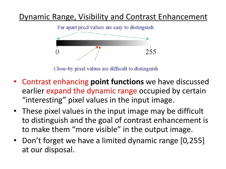
Dynamic Range, Visibility and Contrast Enhancement

• Contrast enhancing point functions we have discussed earlier expand the dynamic range occupied by certain “interesting” pixel values in the input image.

• These pixel values in the input image may be difficult to distinguish and the goal of contrast enhancement is to make them “more visible” in the output image.

• Don’t forget we have a limited dynamic range [0,255] at our disposal.

Neighborhood of size 3 X 3 about a point (x, y) in an image.

x แทนดชันีของแถว y แทนดชันีของคอลมัน์

Intensity Transformation

• โดยทัว่ไปในการแปลงสปาเทียลโดเมน ฟังก์ชนัตา่งๆ สามารถเขียนอยูใ่นรูปงา่ยๆ คือ

s = T(r)

• โดยท่ี r แทนคา่ความเข้มของข้อมลูภาพ f

• สว่น s เป็นคา่ความเข้มในฟังก์ชนั g

• โดยทัง้ r และ s จะอ้างถงึต าแหนงของจดุภาพ (x, y) ท่ีสอดคล้องกนั

basic gray-level transformation

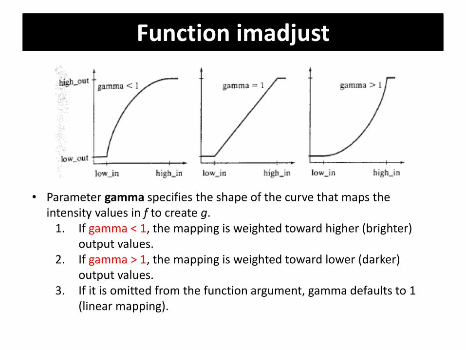
Function imadjust

• imadjust Adjust image intensity values or colormap and syntax:

g = imadjust(f, [low_in high_in], [low_out high_out], gamma)

• ฟังก์ชนันี ้map คา่ความเข้มของภาพ f ไปเป็นคา่ใหม่ g, • ตวัแปร low_in และ high_in คือพิสยัของภาพอินพตุ f จะถกูแม็พไป

ยงัคา่ใหม่ท่ีอยูใ่นช่วง low_out และ high_out • คา่ท่ีต ่ากวา่ low_in จะถกูแม็พไปยงัคา่ low_out สว่นคา่ท่ีสงูกวา่

high_in ก็จะถกูตดัแม็พลงมาท่ี high_out

Continuous and quantized image contrast enhancement.

[low_in high_in]

[lo

w_o

ut

h

igh

_ou

t]

Function imadjust

• Parameter gamma specifies the shape of the curve that maps the intensity values in f to create g.

1. If gamma < 1, the mapping is weighted toward higher (brighter) output values.

2. If gamma > 1, the mapping is weighted toward lower (darker) output values.

3. If it is omitted from the function argument, gamma defaults to 1 (linear mapping).

>>g1=imadjust(f, [0 1], [1 0]); >>g2=imadjust(f, [0.50 .75], [0 1]); >>g3=imadjust(f, [ ], [ ], 2);

100 200 300 400

100

200

300

400

500

Negative images

100 200 300 400

100

200

300

400

500

Expanding intensity range [0.5, 0.75]

100 200 300 400

100

200

300

400

500

Enhancing by gamma=2

100 200 300 400

100

200

300

400

500

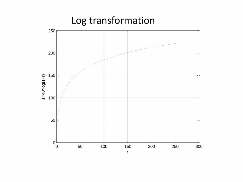
Logarithmic and Contrast-Stretching Transformations

• Logarithmic and contrast-stretching transformations are basic tools for dynamic range manipulation. For example, it is not unusual to have a Fourier spectrum with values in the range [0, 106] or higher.

• Logarithm transformations are implemented using the expression

g = c*log(1 + double(f)) where c is a constant.

• The shape of this transformation is similar to the gamma curve with the low values set at 0 and the high values set to 1 on both scales.

• Note, however, that the shape of the gamma curve is variable, whereas the shape of the log function is fixed.

0 50 100 150 200 250 3000

50

100

150

200

250

r

s=

40*l

og(1

+r)

Log transformation

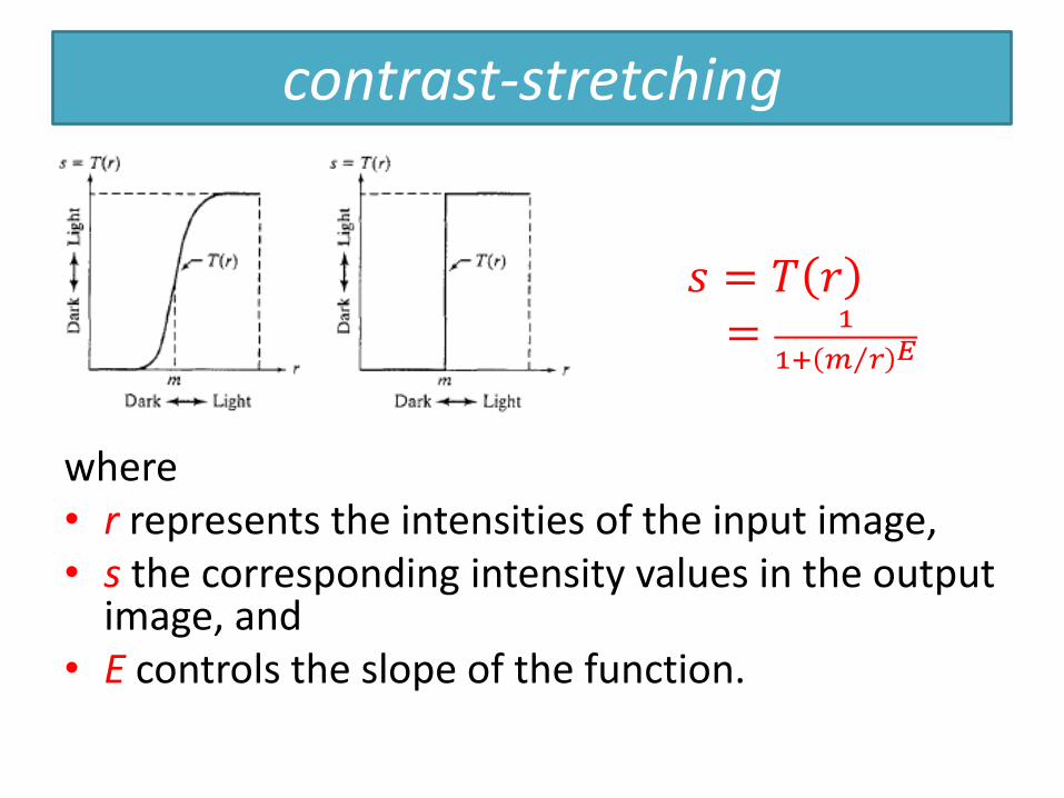
contrast-stretching

where • r represents the intensities of the input image, • s the corresponding intensity values in the output

image, and • E controls the slope of the function.

𝑠 = 𝑇 𝑟 = 1

1+ 𝑚 𝑟 𝐸

Fourier spectrum

50 100 150 200 250

50

100

150

200

2500

1000

2000

3000

4000

5000

6000

7000

Histogram

0 50 100 150 200 250

Log transformation

50 100 150 200 250

50

100

150

200

250

Contrast at m=10,E=2

50 100 150 200 250

50

100

150

200

250

Histogram Processing

• กระบวนการ(Process) แปลงคา่ความเข้ม โดยอาศยัสารสนเทศจากฮิสโทแกรมคา่ความเข้มของภาพ ซึง่เป็นขัน้ตอนพืน้ฐานของการประมวลผลภาพเพ่ือใช้ในงานตา่งๆ เชน่

–enhancement,

–compression,

–segmentation, and

–description

ชนิดของข้อมลูภาพท่ีมีการแจกแจงแตกต่างกนั 1. ภาพมืด เกิดจากข้อมลูของจดุภาพมี

การกระจายตวักระจกุอยู่ท่ีกลุม่ของเฉดท่ีมืด

2. ในทางตรงกนัข้ามถ้า pixels ไปกระจดุอยู่ในย่านของเฉดสีท่ีใกล้กบัสีขาว ภาพก็จะสวา่งมาก

3. ภาพท่ีมีคอนทราสต์ต ่า pixels จะไปกระจดุตวัอยู่ในช่วงแคบๆ

4. ภาพท่ีมีคอนทราสต์มากจะมีความคมชดั

ฮิสโทแกรมข้อมลูภาพ

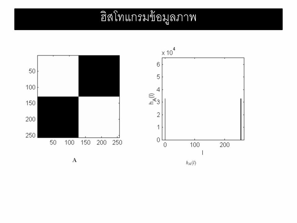
ฮิสโทแกรมข้อมลูภาพ

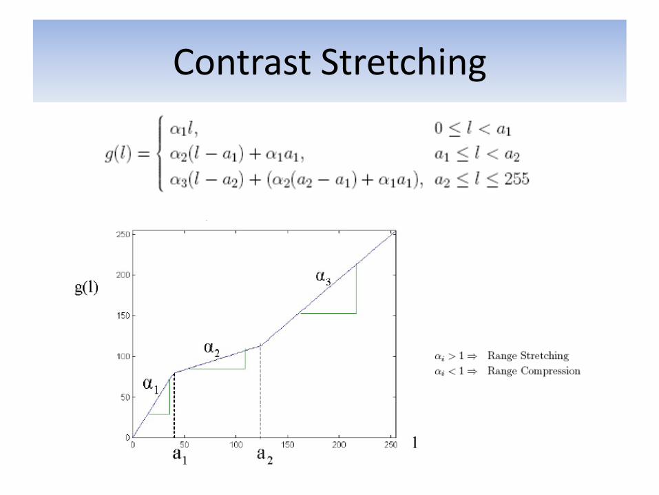
Contrast Stretching

Reduce dynamic range

A “Discontinuous” Point Function

Normalizing an Image

การสร้างฮิสโทแกรมข้อมลูภาพ

• The histogram of a digital image with L total possible intensity levels in the range [0, G] is defined as the discrete function

h(x) = n

เมือ่ x เป็นค่าความเข้มของจุดภาพ x[0,G]

n เป็นจ านวนจุดภาพทีมี่ค่าความเขม้ x • เม่ือต้องการสร้างฮิสโทแกรมของข้อมลูภาพ f ท่ีมีขนาด MxN ก็สามารถ

สร้างได้ดงันี ้– imSize = M*N; – h = zeros(1,MaxGray); – for i=1:imSize

• h(f(i)) = h(f(i)) + 1; %เมื่อ MaxGray ของภาพแปดบิตเทา่กบั 256

h = imhist(f, b) p = imhist(f, b)/numel(f)

Histogram Equalization • r เป็นตวัแปรสุม่ ฟังก์ชนัความหนาแน่นความน่าจะเป็น (Probability

Density Function: PDF) คือ pr(r) • เม่ือท าการแปลงตอ่ไป เพ่ือให้ได้คา่ความเข้ม s ก็จะได้วา่

𝑠 = 𝑇 𝑟 = 𝑝𝑟 𝑤 𝑑𝑤𝑟

0

โดยที่ w เป็น dummy variable ของการอินติเกรต • ดงันัน้ pdf ของ s จะมีการแจกแจงแบบยนูิฟอร์มดงันี ้

𝑝𝑠 𝑠 = 1, 𝑓𝑜𝑟 0 ≤ 𝑠 ≤ 10, otherwise

• The net result of this intensity-level equalization process is an image with increased dynamic range, which will tend to have higher contrast.

• Transformation function is really nothing more than the Cumulative Distribution Function (CDF).

Histogram Equalization

• For discrete quantities we work with summations, and the equalization transformation becomes

𝑠𝑘 = 𝑇 𝑟𝑘 = 𝑝𝑟(𝑟𝑗)𝑘𝑗=0

= 𝑛𝑗

𝑛𝑘𝑗=0 , 𝑘 = 0,1,2, … , 𝐿 − 1

• Histogram equalization is implemented in the toolbox by function histeq, which has the syntax

g = histeq(f, nlev)

100 200 300 400 500

100

200

300

400

5000

2000

4000

6000

0 100 200

100 200 300 400 500

100

200

300

400

5000

2000

4000

6000

0 100 200

>>figure; >>subplot(2,2,1); >>image(f); >>subplot(2,2,2); >>imhist(f); >>g=histeq(f); %nlev=64 >>subplot(2,2,3); >>image(g); >>subplot(2,2,4); >>imhist(g);

g=histeq(f,max(f(:)))

100 200 300 400 500

100

200

300

400

500

g=histeq(f,256)

100 200 300 400 500

100

200

300

400

5000

2000

4000

6000

imhist(g)0 100 200

0

2000

4000

6000

0 100 200

100 200 300 400 500

100

200

300

400

500

0 100 200 3000

0.5

1

1.5

r

cdf(

r)

0 100 200 3000

0.02

0.04

0.06

0.08

r

p(r

)

0 100 200 3000

50

100

150

200

250

300

r

s=

cdf(

r)*2

55

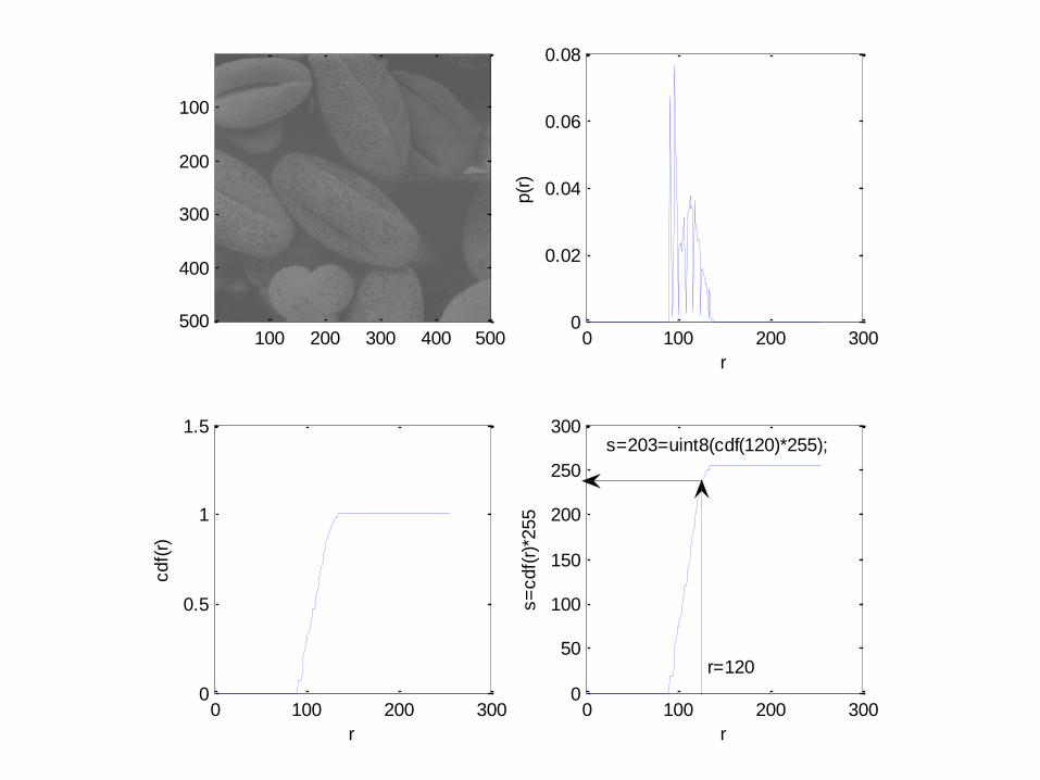
r=120

s=203=uint8(cdf(120)*255);

Histogram Equalization

𝑝𝑟(𝑟𝑗)

𝑘

𝑗=0

𝑝𝑟(𝑟𝑗)

r Uniform

Quantization %S=cdf(r)*L

s

for i=1:M for j=1:N g(i,j) = cdf(f(i,j))*255; end end

50 100 150 200 250 300 350 400 450 500

50

100

150

200

250

300

350

400

450

500

>>g = uint8(reshape(s(f),[size(f)]));

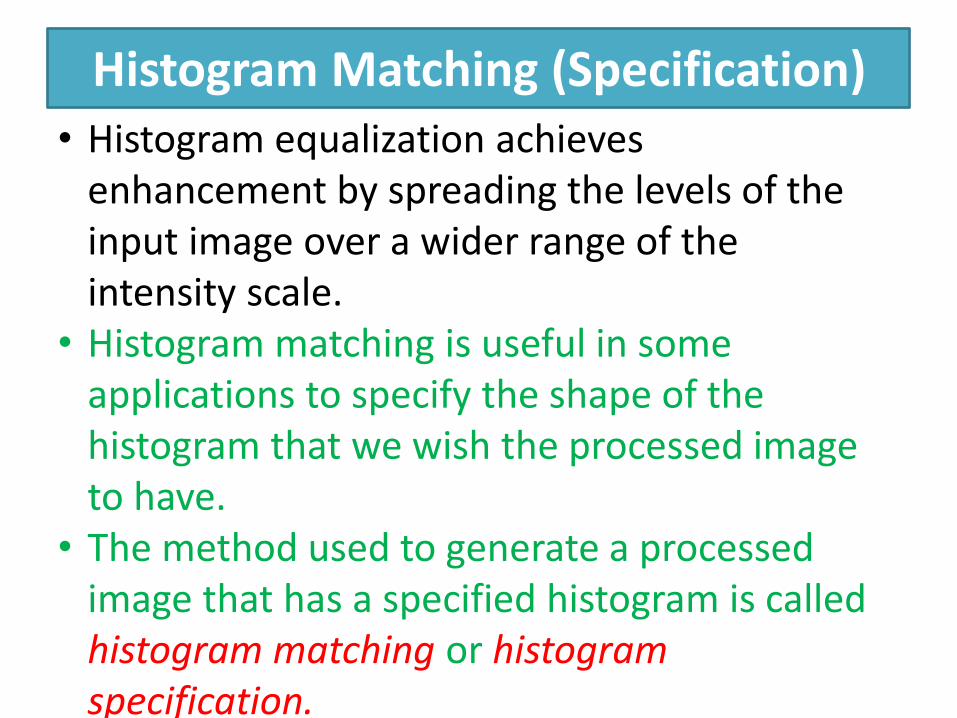
Histogram Matching (Specification) • Histogram equalization achieves

enhancement by spreading the levels of the input image over a wider range of the intensity scale.

• Histogram matching is useful in some applications to specify the shape of the histogram that we wish the processed image to have.

• The method used to generate a processed image that has a specified histogram is called histogram matching or histogram specification.

Histogram Specification

• Consider for a moment continuous levels that are normalized to the interval [0,1], and let u and v denote the intensity levels of the input and output images.

• The input levels have pdf, Pu(u) and the output levels have the specified pdf, pv(v).

Histogram Specification

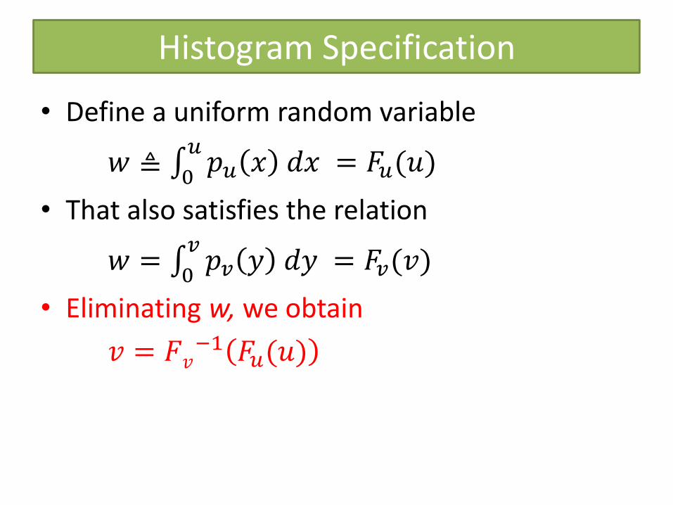
• Define a uniform random variable

𝑤 ≜ 𝑝𝑢 𝑥 𝑑𝑥 𝑢

0= 𝐹𝑢(𝑢)

• That also satisfies the relation

𝑤 = 𝑝𝑣 𝑦 𝑑𝑦 𝑣

0= 𝐹𝑣(𝑣)

• Eliminating w, we obtain

𝑣 = 𝐹𝑣−1 𝐹𝑢(𝑢)

Histogram specification

0

1

2

3

4

5

x 104

0 50 100 150 200 250

Mars moon, its histogram, obtained using imhist (f). The image is dominated by large, dark areas, resulting in a histogram characterized by a large concentration of pixels in the dark end of the gray scale.

100 200 300 400 500 600

100

200

300

400

500

600

700

800

900

10000 100 200 300

0

0.5

1

1.5

2

2.5

3

3.5

4x 10

5

Histogram Equalization would be a good approach to enhance this image, so that details in the dark areas become more visible. >> g = histeq(f, 256); Shows that histogram equalization in fact did not produce a particularly good result in this case as seen from its histogram(in red), the blue one is cdf*max(imhist(f)).

0

1

2

3

4

5

x 104

0 50 100 150 200 250100 200 300 400 500 600

100

200

300

400

500

600

700

800

900

1000

0 50 100 150 200 250 3000

0.1

0.2

0.3

0.4

0.5

0.6

0.7

0 50 100 150 200 250 3000

0.002

0.004

0.006

0.008

0.01

0.012

0.014

0.016

0.018

0.02

PDF of image f

Generate new PDF, p

>> g = histeq(f, p);

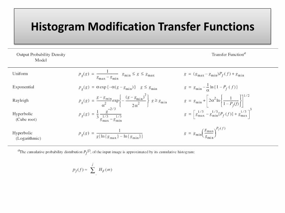
Histogram Modification Transfer Functions

0 100 200 3000

1

2

3

4

5

6

7x 10

-3

0 100 200 3000

0.2

0.4

0.6

0.8

1

Intensity

CD

F

0 100 200 30050

100

150

200

Original intesity

Modefied inte

nsity

x=0:255; gmin = 50; gmax = 200; in = find(x>gmin & x<gmax); u = zeros(1,256); u(in) = u(in)+ones(size(in)); subplot(2, 2, 1),plot(u) xlabel('Intensity'); ylabel('Uniform pdf'); u=u/(gmax-gmin); plot(u) cdf = cumsum(u); subplot(2, 2, 2),plot(cdf) xlabel('Intensity'); ylabel('CDF'); g = (gmax-gmin)*cdf+gmin; subplot(2,2,3), plot(g) xlabel('Original intesity'); ylabel('Modefied intensity'); newIm = f; inx = find(f>gmin & f<gmax); newIm(inx) = (gmax-gmin)*cdf(f(inx))+gmin; subplot(2,2,4),imshow(newIm);

Histogram hyperbolization

neighborhood processing

The process of moving the center point creates new neighborhoods, one for each pixel in the input image. • The two principal terms used to identify this

operation are neighborhood processing and spatial filtering, with the second term more being prevalent.

• As explained in the following section, if the computation performed on the pixels of the neighborhoods are linear, – the operation is called linear spatial filtering (the

term spatial convolution also used); – otherwise, it is called nonlinear spatial filtering.

BASIC TERMINOLOGY

(a)4-neighborhood; (b) diagonal neighborhood; (c) 8-neighborhood.

• The process consists

simply of moving the center of the filter mask w from point to point in an image, f.

• At each point (x, y), the response of the filter at that point is the sum of

products of the filter coefficients and the corresponding neighborhood pixels in the area spanned by the filter mask.

• For a mask of size m × n,

we assume typically that m = 2a + 1 and n = 2b + 1, where a and b are

nonnegative integers.

Spatial Filtering

Spatial filtering is a neighborhood processing consisting of:

1. defining a center point, (x, y);

2. performing an operation that involves only the pixels in a predefined neighborhood about that center point;

3. letting the result of that operation be the "response" of the process at that point;

4. repeating the process for every point in the image.

Filtering • Linear Filters: The resulting output pixel is computed

as a sum of products of the pixel values and mask coefficients in the pixel’s neighborhood in the original image. Example: mean filter.

• Nonlinear Filters: The resulting output pixel is selected from an ordered (ranked) sequence of pixel values in the pixel’s neighborhood in the original image. Example: median filter.

If the neighborhood is of size m × n, mn coefficients are required. The coefficients are arranged as a matrix, called a filter, mask, filter mask, kernel, template, or window, with the first three terms being the most prevalent. For reasons that will become obvious shortly, the terms convolution filter, mask, or kernel, also are used.

CONVOLUTION • In one-dimensional

𝐴 ∗ 𝐵 = 𝐴 𝑗 ∙ 𝐵 𝑥 − 𝑗

∞

𝑗=−∞

• Ex: Let A = {0, 1, 2, 3, 2, 1, 0}, and B = {1, 3,−1}.

1. A(x=1)

(0 × (−1)) + (0 × 3) + (1 × 1) = 1

CONVOLUTION (cont.)

⋮

7. A(x=7)

(0 × (−1)) + (1 × 3) + (2 × 1) = 5

2. A(x=2)

(1 × (−1)) + (0 × 3) + (0 × 1) = −1

2D Convolution

𝑔 𝑥, 𝑦 = 𝑤 𝑘, 𝑙 𝑓(𝑥 − 𝑘, 𝑦 − 𝑙)

𝑛/2

𝑙=−𝑛/2

𝑚/2

𝑘=−𝑚/2

EXAMPLE

2D Convolution

Spatial Averaging and Spatial Low-Pass Filtering

แตล่ะจดุภาพจะถกูปรับปรุงโดย คา่เฉล่ียถ่วงน า้หนกัจากจดุภาพในบริเวณใกล้เคียง นัน่คือ

𝑔 𝑥, 𝑦 = 𝑤 𝑘, 𝑙 𝑓(𝑥 − 𝑘, 𝑦 − 𝑙)

𝑛

𝑙=1

𝑛

𝑘=1

เม่ือ g และ f เป็นภาพเอาต์พตุและอินพตุตามล าดบั n เป็นขนาดของวินโดว์ w คือแมทิกซ์คา่ถ่วงน า้หนกั ในการกรองสญัญาณภาพด้วยตวักรองที่คา่ถ่วงน า้หนกัทกุตวัเทา่กบัหนึง่ก็จะได้จดุภาพโดยเฉลี่ยในวินโดว์

𝑔 𝑥, 𝑦 =1

𝑁𝑤 𝑓(𝑥 − 𝑘, 𝑦 − 𝑙)

𝑛

𝑙=1

𝑛

𝑘=1

โดยที่ 𝑤 = 1 𝑁𝑤 และ 𝑁𝑤 คือจ านวนสมาชิกของวินโดว์ w

Spatial Averaging and Spatial Low-Pass Filtering

การกรองข้อมลูภาพสามารถเขียนได้อีกแบบหนึง่คือ 𝑔 𝑥, 𝑦 =

1

2 𝑓 𝑥, 𝑦

+1

4𝑓 𝑥 − 1, 𝑦 + 𝑓 𝑥 + 1, 𝑦 + 𝑓 𝑥, 𝑦 − 1 + 𝑓(𝑥, 𝑦 + 1)

𝑤1 =1 11 1

, 𝑤2 =1 1 11 1 11 1 1

, 𝑤3 =

0 14 0

14

12

14

0 14

0

𝑔 𝑥, 𝑦 =1

𝑁𝑤 𝑤1 𝑘, 𝑙 𝑓 𝑥 − 𝑘, 𝑦 − 𝑙

𝑛

𝑙=1

𝑛

𝑘=1

=1

4 𝑓 𝑥 − 𝑘, 𝑦 − 𝑙

𝑛

𝑙=1

𝑛

𝑘=1

=1

4𝑓 𝑥, 𝑦 + 𝑓 𝑥, 𝑦 − 1 + 𝑓 𝑥 − 1, 𝑦 + 𝑓 𝑥 − 1, 𝑦 − 1

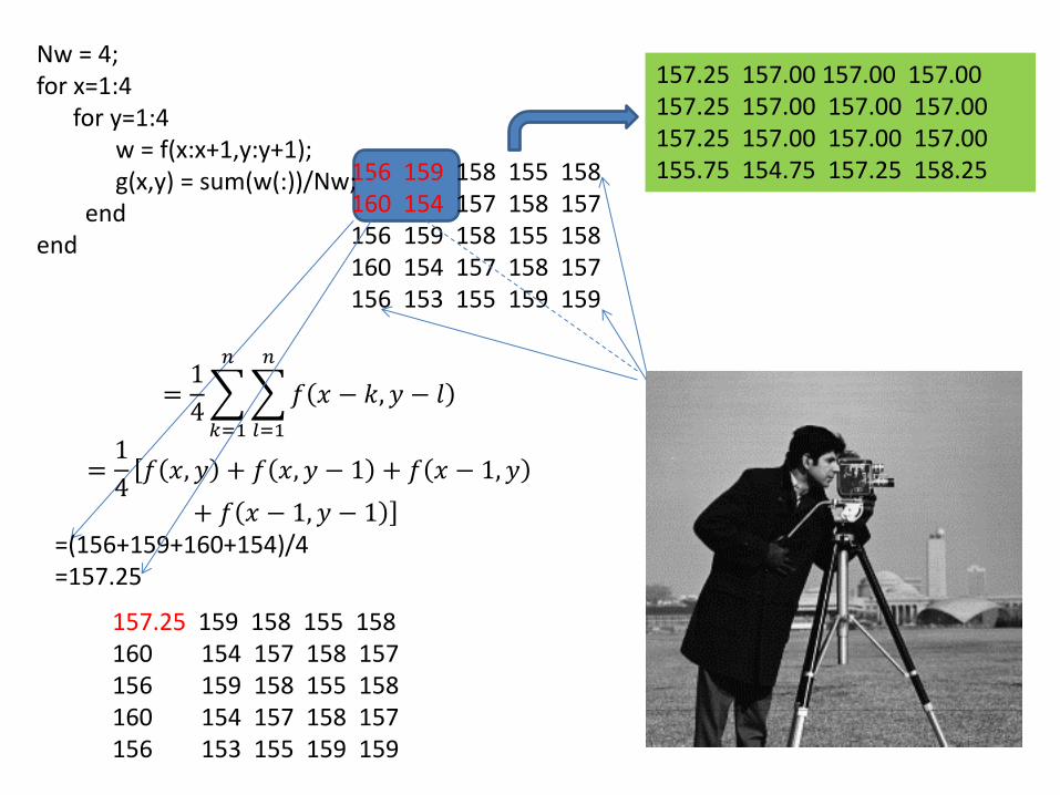
156 159 158 155 158 160 154 157 158 157 156 159 158 155 158 160 154 157 158 157 156 153 155 159 159

Nw = 4; for x=1:4 for y=1:4 w = f(x:x+1,y:y+1); g(x,y) = sum(w(:))/Nw; end end

=1

4 𝑓 𝑥 − 𝑘, 𝑦 − 𝑙

𝑛

𝑙=1

𝑛

𝑘=1

=1

4 𝑓 𝑥, 𝑦 + 𝑓 𝑥, 𝑦 − 1 + 𝑓 𝑥 − 1, 𝑦

+ 𝑓 𝑥 − 1, 𝑦 − 1 =(156+159+160+154)/4 =157.25

157.25 157.00 157.00 157.00 157.25 157.00 157.00 157.00 157.25 157.00 157.00 157.00 155.75 154.75 157.25 158.25

157.25 159 158 155 158 160 154 157 158 157 156 159 158 155 158 160 154 157 158 157 156 153 155 159 159

Variations of averaging filter

Modified Mask Coefficients

Variations of averaging filter

a, b, c, d a) Original image b) 3x3 average c) Modified Mask

Coefficients

d) Gaussian blur filter, 𝜎 = 0.5

ℎ =0.0113 0.0838 0.0113 0.0838 0.6193 0.08380.0113 0.0838 0.0113

Low-pass filtering การกรองข้อมลูภาพด้วยการเฉลี่ยกบัจดุภาพบริเวณใกล้เคียง ถกูใช้เพ่ือลดสญัญาณรบกวน (Noise) ซึง่บางครัง้ก็จะเรียกวา่ “การกรองความถ่ีต ่าผ่าน (Low-pass filterer)” เน่ืองจากภาพดิจิทลั f โดยทัว่ไปจะแทนอยูใ่นรูป 𝑓 𝑥, 𝑦 = 𝑢 𝑥, 𝑦 + 𝜂(𝑥, 𝑦) โดยที่ 𝑢 𝑥, 𝑦 เป็นสญัญาณภาพที่ไมม่ีสญัญาณรบกวน 𝜂(𝑥, 𝑦) ซึง่เป็น white noise ที่มีคา่เฉลี่ยเทา่กบัศนูย์และความแปรปรวนเทา่กบั ท าให้การหาคา่เฉล่ียของจดุภาพข้างต้นกลายเป็น

𝑔 𝑥, 𝑦 =1

𝑁𝑤 𝑓(𝑥 − 𝑘, 𝑦 − 𝑙)

𝑛

𝑙=1

𝑛

𝑘=1

=1

𝑁𝑤 𝑢 𝑥 − 𝑘, 𝑦 − 𝑘 + 𝜂 𝑥 − 𝑘, 𝑦 − 𝑘 𝑛

𝑙=1𝑛𝑘=1

=1

𝑁𝑤 𝑢 𝑥 − 𝑘, 𝑦 − 𝑙 +𝑛

𝑙=1 𝜂 (𝑥, 𝑦)𝑛𝑘=1

2

การก าจดัสญัญาณรบกวน

g 𝑥, 𝑦 =1

𝑁𝑤 𝑢 𝑥 − 𝑘, 𝑦 − 𝑙 +

𝑛

𝑙=1

𝜂 (𝑥, 𝑦)

𝑛

𝑘=1

เม่ือ 𝜂 (𝑥, 𝑦) เป็นคา่เฉลี่ยของสญัญาณรบกวน 𝜂(𝑥, 𝑦) ท่ีมีคา่เฉลี่ยเท่าศนูย์และความแปรปรวนเท่ากบั

จะเห็นวา่สญัญาณรบกวนถกูลดด้วยจ านวนสมาชิกของวินโดว์ w แต่ในทางปฏิบตัิเราไมส่ามารถเพิ่มขนาดของวินโดว์ w ให้ใหญ่มากๆ ได้ เน่ืองจากจะท าให้ภาพเบลอมากตามขนาดของวินโดว์ท่ีใหญ่ขึน้ ดงัจะเห็นจากตวัอยา่งตอ่ไปนี ้

2 2

wN

Original noise,var=0.1 average with 3x3

average with 5x5 average with 7x7 average with 9x9

Smoothing image containing Gaussian noise

Median filtering

จดุภาพอินพตุจะถกูแทนท่ีด้วยคา่มธัยฐาน (Median) จากวินโดว์

𝑔 𝑥, 𝑦 = 𝑚𝑒𝑑𝑖𝑎𝑛 𝑓 𝑥 − 𝑘, 𝑦 − 𝑙 , (𝑘, 𝑙) ∈ 𝑊

เม่ือวินโดว์ W ถกูก าหนดขนาดอยา่งเหมาะสม Algorithm ของการกรองด้วยคา่มธัยฐานจะต้องมีการจดัเรียงคา่ความเข้มของจดุภาพใน W อาจจะเรียงจากน้อยไปหามากหรือมากไปหาน้อยก็ได้ ตอ่จากนัน้ก็จะดงึเอาคา่ตรงกลางมาก าหนดให้ g(x,y) ในแตล่ะจดุ โดยทัว่ไปจะก าหนดขนาดวินโดว์ให้มีจ านวนสมาชิกเป็นเลขคี่ เช่น 3×3, 5× 5, 7 × 7 เป็นต้น ในกรณีนีส้ามารถดงึสมาชิกของ W ท่ีเรียงล าดบัแล้วมาได้เลย แตถ้่า สมาชิกของ W เป็นจ านวนคูค่า่ g(x,y) จะถกูก าหนดจากคา่เฉลี่ยของสมาชิก W ท่ีอยูก่ึ่งกลางสองตวั

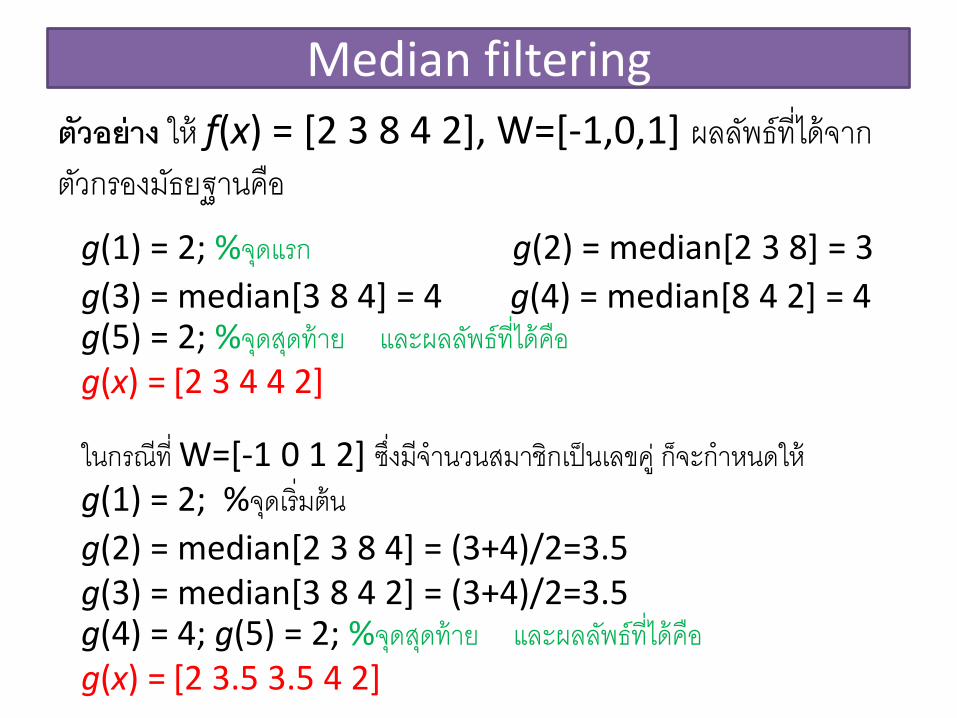
Median filtering

ตัวอย่าง ให้ f(x) = [2 3 8 4 2], W=[-1,0,1] ผลลพัธ์ท่ีได้จากตวักรองมธัยฐานคือ

g(1) = 2; %จดุแรก g(2) = median[2 3 8] = 3

g(3) = median[3 8 4] = 4 g(4) = median[8 4 2] = 4 g(5) = 2; %จดุสดุท้าย และผลลพัธ์ท่ีได้คือ g(x) = [2 3 4 4 2]

ในกรณีท่ี W=[-1 0 1 2] ซึง่มีจ านวนสมาชิกเป็นเลขคู ่ก็จะก าหนดให้ g(1) = 2; %จดุเร่ิมต้น

g(2) = median[2 3 8 4] = (3+4)/2=3.5 g(3) = median[3 8 4 2] = (3+4)/2=3.5 g(4) = 4; g(5) = 2; %จดุสดุท้าย และผลลพัธ์ท่ีได้คือ g(x) = [2 3.5 3.5 4 2]

A Noisy Step Edge

0 10 20 30 40 50 60 700

0.2

0.4

0.6

0.8

1

1.2

1.4

1.6

1.8

[1: 70];

;

where

unifrnd 0.25 , 0.25,1,70

H

Hn H u

u

0.25 for 35

1.25 for 35

nH n

n

0 10 20 30 40 50 60 700

0.2

0.4

0.6

0.8

1

1.2

1.4

1.6

1.8

Blurred Noisy 1D Step Edge

4

4

1

9 k

h n H n k

0 10 20 30 40 50 60 700

0.2

0.4

0.6

0.8

1

1.2

1.4

1.6

1.8

Blurred Noisy 1D Step Edge

Hn(34-4:34+4)= 0.6008

0.0219

0.6966

0.5477

0.3665

1.4339

1.1780

1.3441

1.7223

Hn(33-4:33+4)=

0.6966

0.5477

0.3665

1.4339

1.1780

1.3441

1.7223

1.4101

1.3909

0.8791

1.1211

mean

mean

0 10 20 30 40 50 60 700

0.2

0.4

0.6

0.8

1

1.2

1.4

1.6

1.8

Median Filtered Noisy 1D Step Edge

4

4med

kh n H n k

0 10 20 30 40 50 60 700

0.2

0.4

0.6

0.8

1

1.2

1.4

1.6

1.8

Median Filtered Noisy 1D Step Edge

Hn(34-4:34+4)=

0.6008

0.0219

0.6966

0.5477

0.3665

1.4339

1.1780

1.3441

1.7223

0.0219

0.3665

0.5477

0.6008

0.6966

1.1780

1.3441

1.4339

1.7223 Hn(35-4:35+4)=

0.0219

0.6966

0.5477

0.3665

1.4339

1.1780

1.3441

1.7223

1.4101

0.0219

0.3665

0.5477

0.6966

1.1780

1.3441

1.4101

1.4339

1.7223

sorted

sorted

median

median

0 10 20 30 40 50 60 700

0.2

0.4

0.6

0.8

1

1.2

1.4

1.6

1.8

Median vs. Blurred

step

noisy

blurred

median

ตวักรองมธัยฐานจะคงสภาพของขอบได้ดีกวา่ ตวักรองคา่เฉลี่ย

Median vs. Average Original

Noise,var=0.1

Median,3x3 Median,5x5

Average,3x3 Average,5x5

คณุสมบตัิของตวักรองมธัยฐาน

• เป็นตวักรองแบบไม่เป็นเชิงเส้น (Nonliner filter) ดงันัน้สองล าดบั x(m) และ y(m) ใดๆ

median(x(m)+y(m)) ≠ median(x(m))+median(y(m))

• ใช้ในการก าจดัสญัญาณรบกวน โดยยงัรักษา spatial resolution ไว้ได้มากกวา่ average filter

• ศกัยภาพในการก าจดัสญัญาณรบกวนจะน้อยลง เม่ือจ านวนของสญัญาณรบกวนในวินโดวส์มากกวา่คร่ึง

Original Noise,var=0.005

Median,3x3 Median,5x5