Internet Economicsכלכלת האינטרנט

Class 10 – it’s a small world

1

Outline

2

• Reminder from last week

• Milgram’s experiment

• Small world phenomena

• A random model of social network

• Some statistics if we have time….

Outline

3

• Last week: we modeled social network as graph, added some natural assumptions and definitions.Motivation: searching for information in the network.

• Today: more specific modeling of social network, emphasis on geographical locations.Motivation: spread of information in social networks (very close to search…)

Modeling Social Networks

4

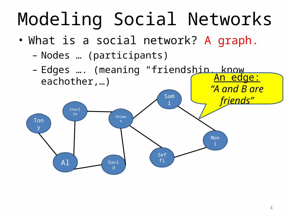
• What is a social network? A graph.– Nodes … (participants)– Edges …. (meaning “friendship, know eachother,…)

Al

Charlie

David

Shimon

Seffi

Sami

Moni

Tony

An edge:“A and B are

friends”

Triadic Closure

5

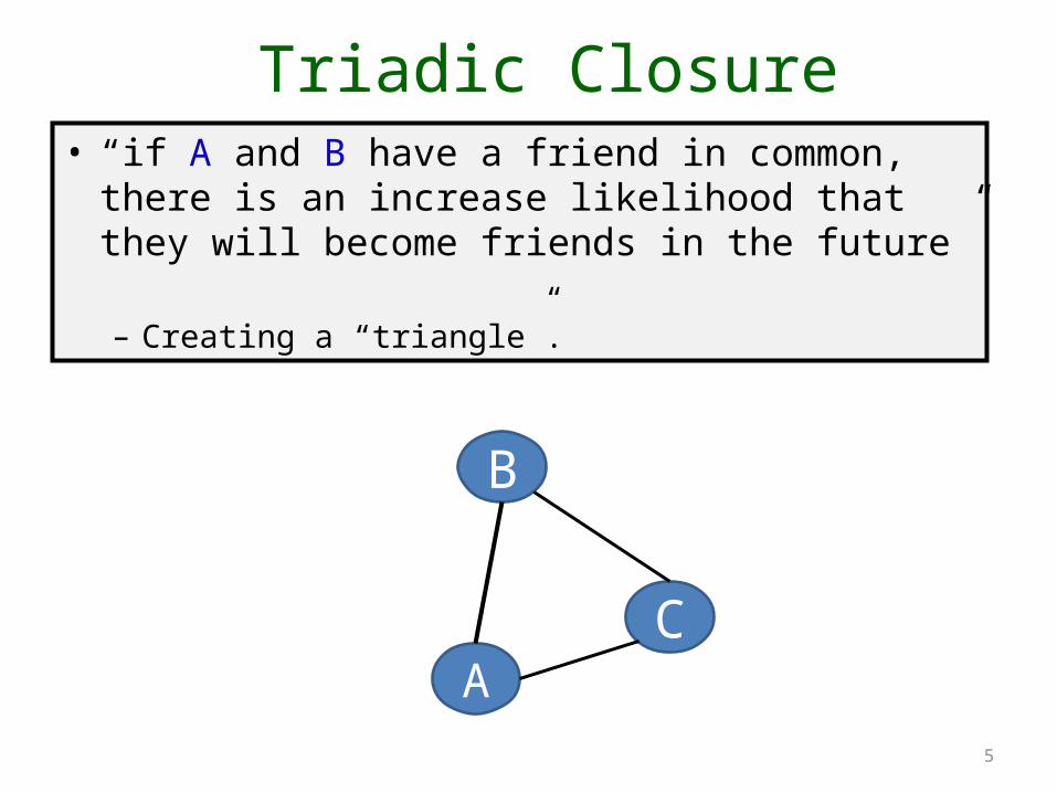
• “if A and B have a friend in common, there is an increase likelihood that they will become friends in the future”– Creating a “triangle”.

A

B

C

Strong/weak ties

6

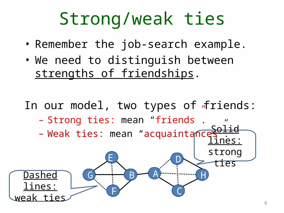
• Remember the job-search example.• We need to distinguish between strengths of

friendships.

In our model, two types of friends:– Strong ties: mean “friends”.– Weak ties: mean “acquaintances”.

G

E

F

B

C

D

HA

Solid lines:strong ties

Dashed lines:weak ties

Outline

7

Graphs: connectivity

8

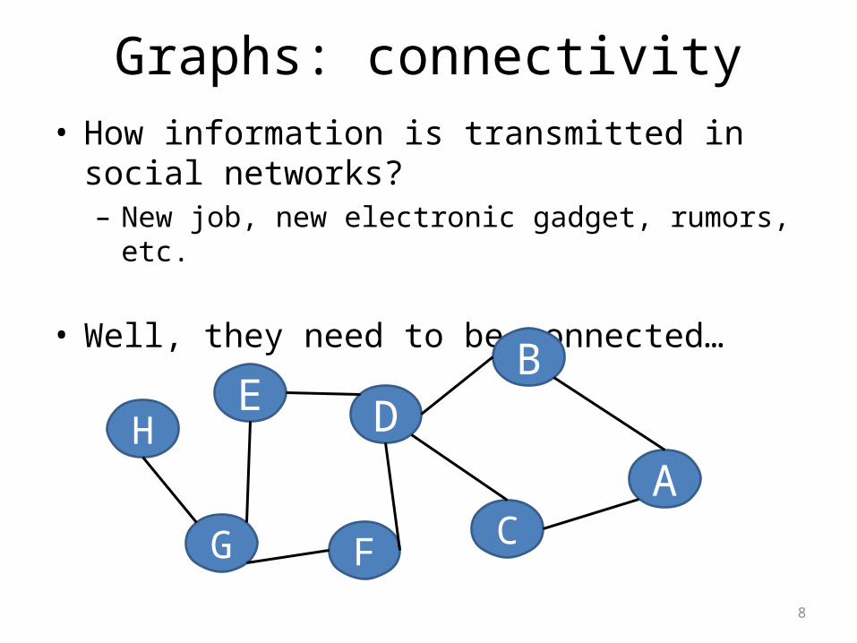
• How information is transmitted in social networks?– New job, new electronic gadget, rumors, etc.

• Well, they need to be connected…

G

E

F

D

C

B

AH

Graphs: connectivity

9

G

E

F

D

C

B

AH

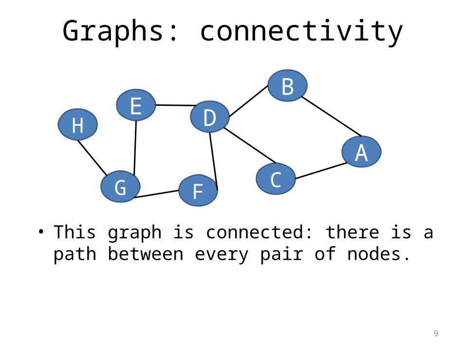
• This graph is connected: there is a path between every pair of nodes.

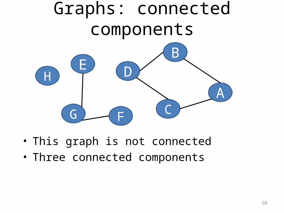
Graphs: connected components

10

G

E

F

D

C

B

AH

• This graph is not connected• Three connected components

Connectivity in social networks

11

• Are social networks connected?– Probably not…– Even one isolated person can cause it– “an isolated tropical island”

• But we can see that real social networks have high connectivity:– usually have a giant component– And usually only one…

• Examples:

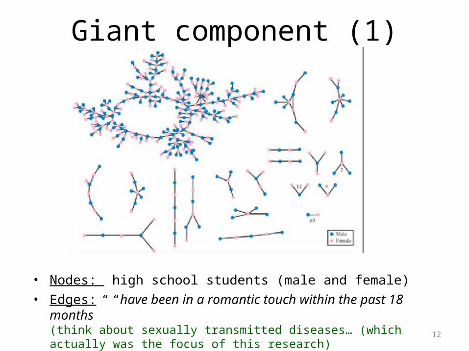
Giant component (1)

12

• Nodes: high school students (male and female)• Edges: “have been in a romantic touch within the past 18 months”

(think about sexually transmitted diseases… (which actually was the focus of this research)

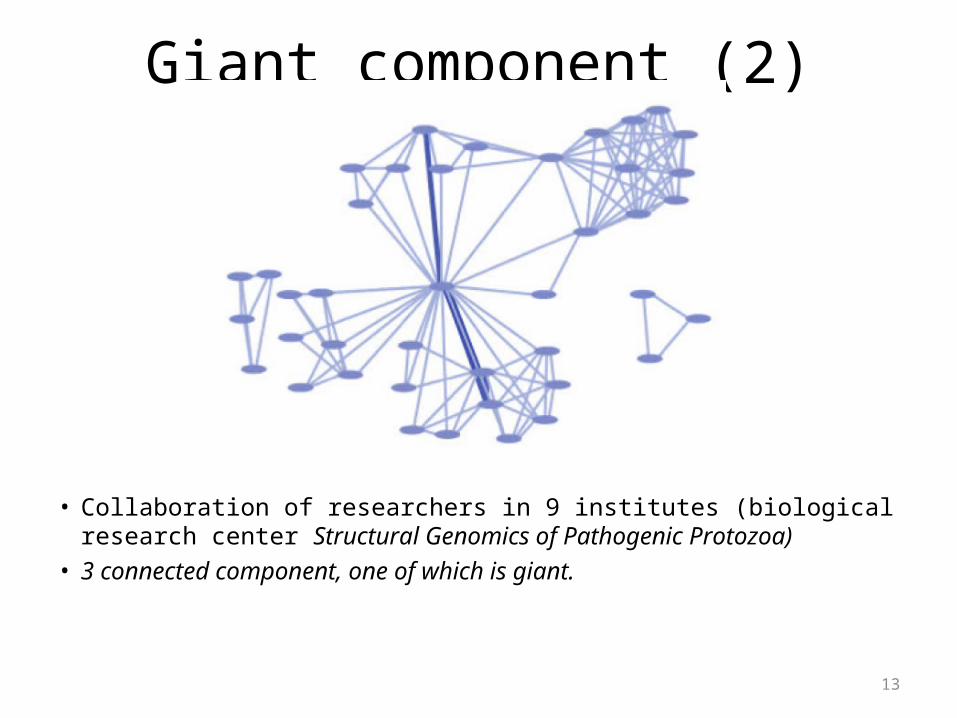
Giant component (2)

13

• Collaboration of researchers in 9 institutes (biological research center Structural Genomics of Pathogenic Protozoa)

• 3 connected component, one of which is giant.

Distances in social networks

14

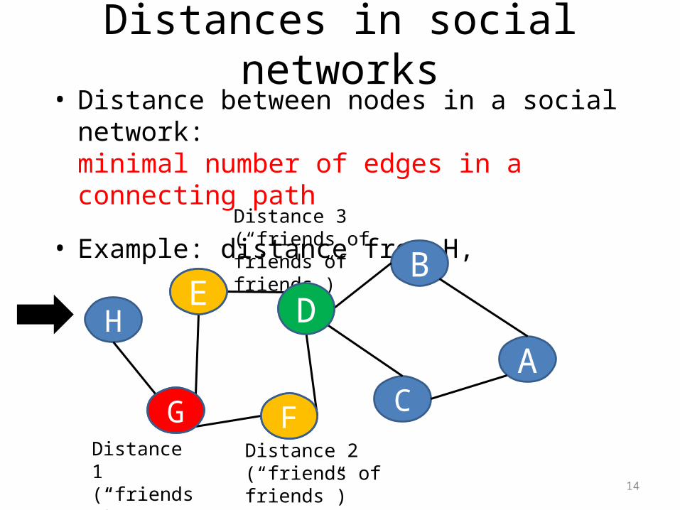
• Distance between nodes in a social network:minimal number of edges in a connecting path

• Example: distance from H,

G

E

F

D

C

B

AH

GDistance 1(“friends”)

E

FDistance 2(“friends of friends”)

Distance 3 (“friends of friends of friends”)

D

Distances

15

• We saw: most of the nodes in social networks lie in a giant connected component.

• But what about the distance between some two nodes? Can it be large?

• Answer: in principle, no.

“small world phenomenon”:not only do you have paths of friends connecting you to a large fraction of the world’s population, but these paths are surprisingly short.

Small world

16

• What lead to this observation?

Experiment (Milgram, 1960’s)

17

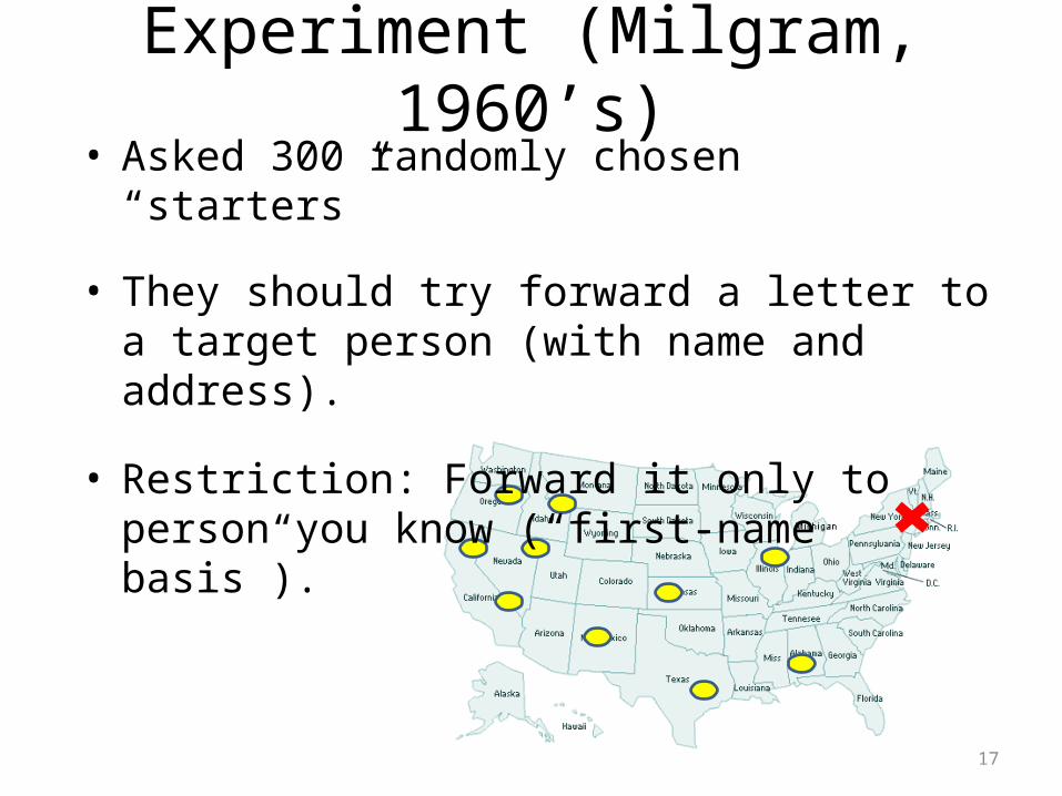
• Asked 300 randomly chosen “starters”

• They should try forward a letter to a target person (with name and address).

• Restriction: Forward it only to person you know (“first-name basis”).

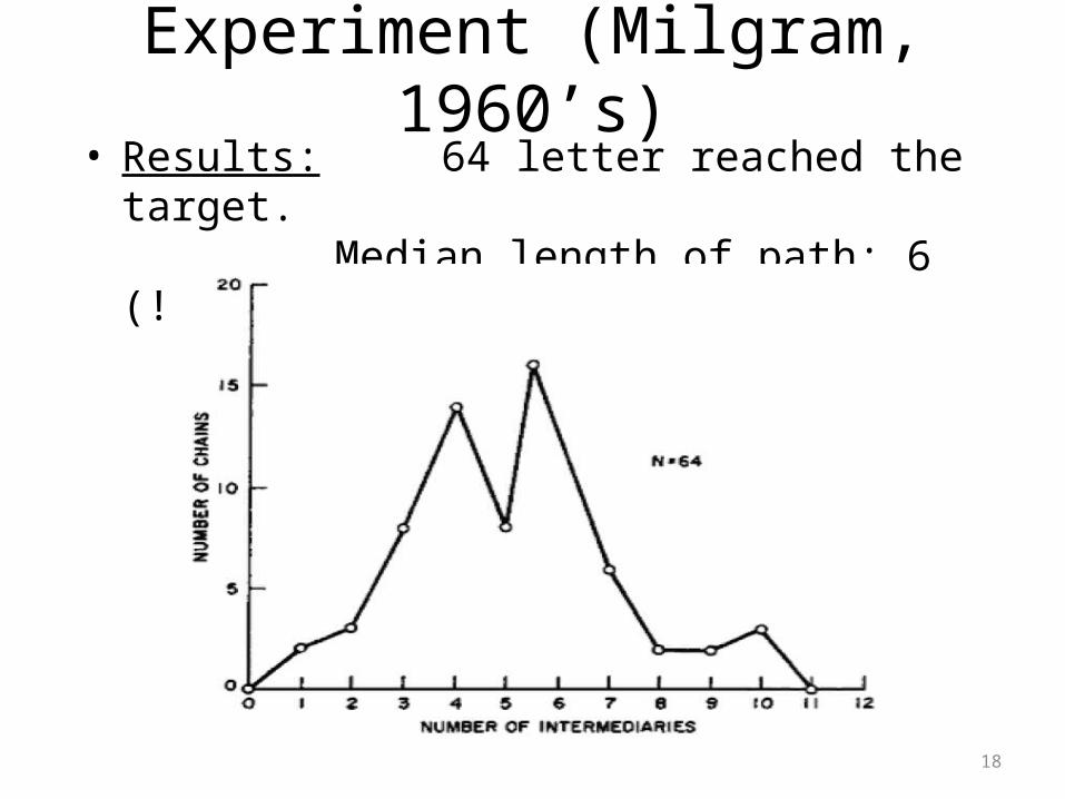
Experiment (Milgram, 1960’s)

18

• Results: 64 letter reached the target.Median length of path: 6 (!)

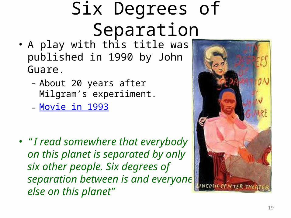
Six Degrees of Separation

19

• A play with this title was published in 1990 by John Guare.– About 20 years after Milgram’s

experiiment.– Movie in 1993

• “I read somewhere that everybody on this planet is separated by only six other people. Six degrees of separation between is and everyone else on this planet”

A more recent experiment

20

• Social network: users of Microsoft Instant Messenger. – Edge: the users communicated at least once over the last

month.– 240 Million active user accounts.

• Results:– A giant component containing almost all the

nodes.– Average distance between nodes: 6.6– Median of distances between nodes: 7

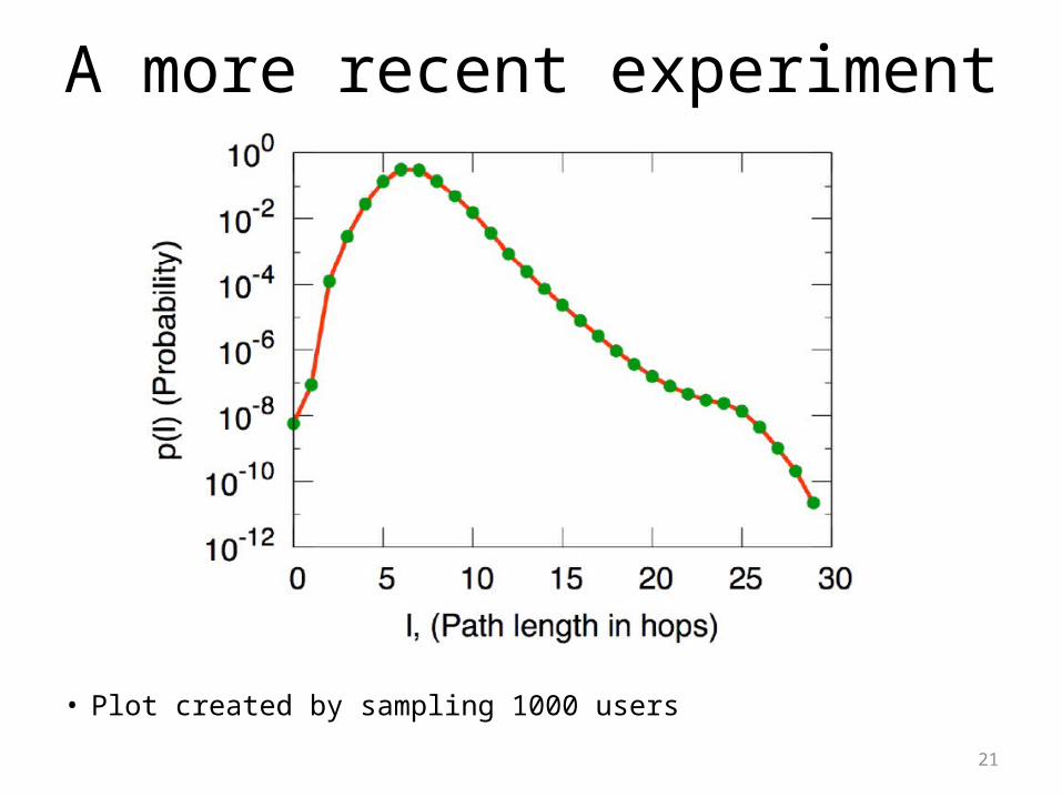
A more recent experiment

21

• Plot created by sampling 1000 users

Experiment conclusion

22

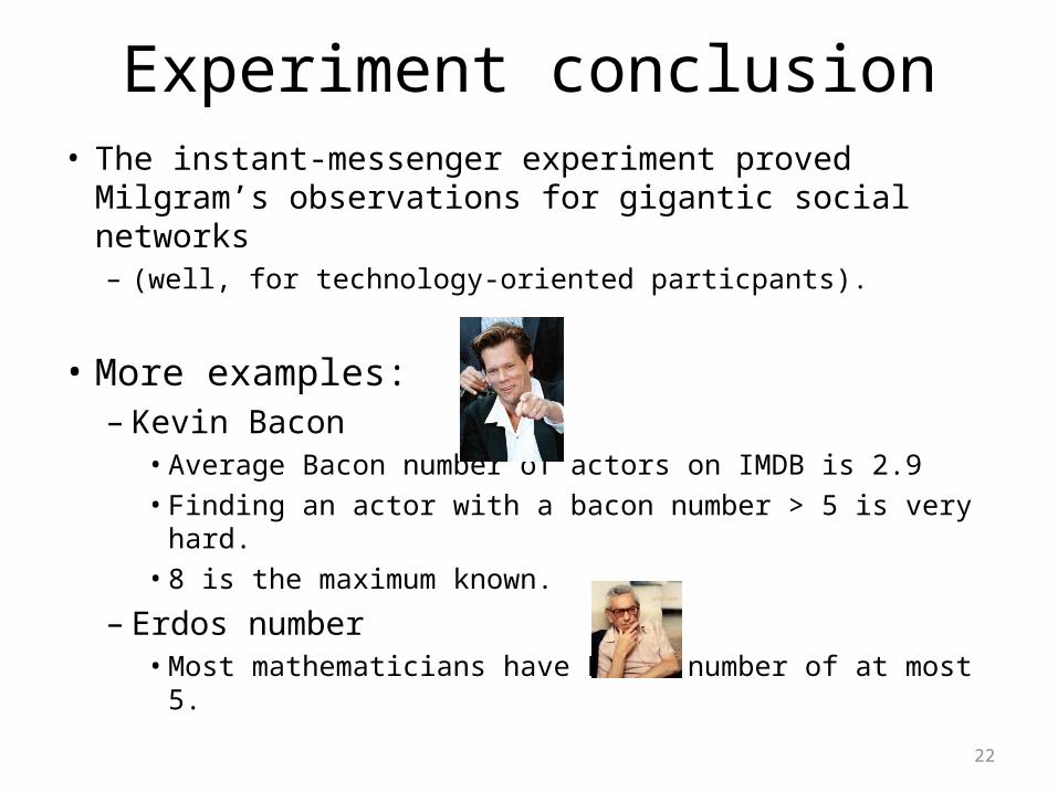
• The instant-messenger experiment proved Milgram’s observations for gigantic social networks– (well, for technology-oriented particpants).

• More examples:– Kevin Bacon

• Average Bacon number of actors on IMDB is 2.9• Finding an actor with a bacon number > 5 is very hard.• 8 is the maximum known.

– Erdos number• Most mathematicians have Erdos number of at most 5.

Distances

23

• So it turns out that distances in social networks are short.

• The more interesting part of Milgram’s experiment:how do people find the short paths?– People decide to forward the message to their

friends, without observing the whole network.– Shortest paths easy search, but only when

flooding is allowed. (In the experiment, each agent forwarded the letter to a single friend.)

Possible reason: exponential expansion

24

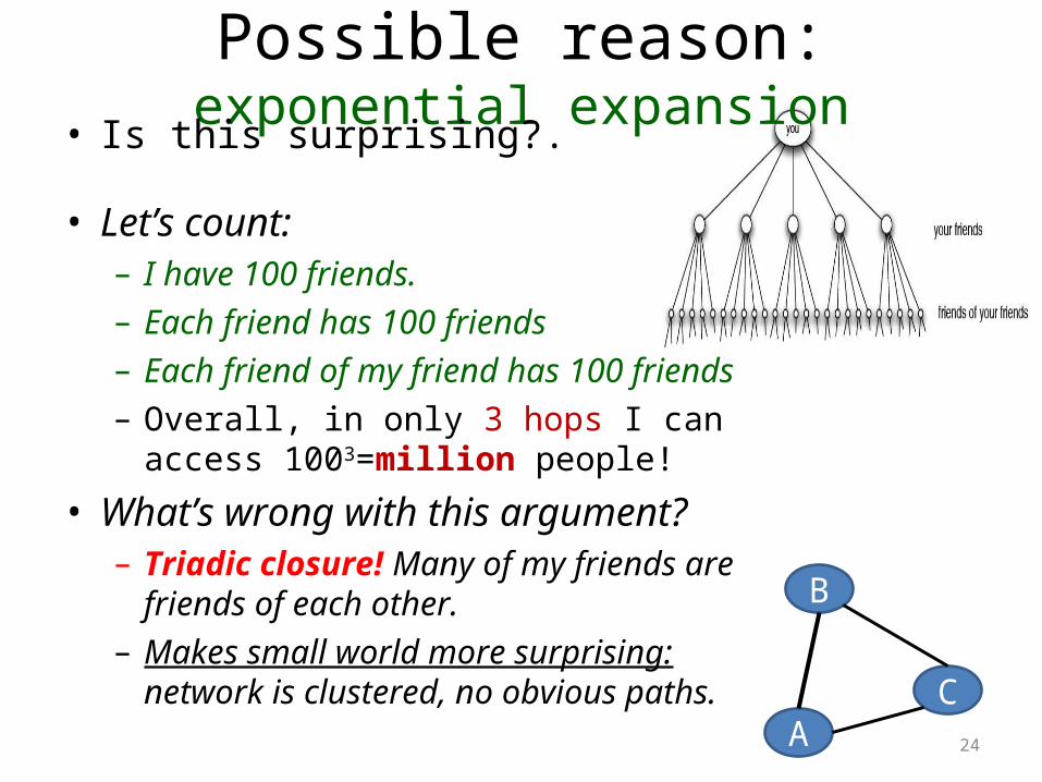
• Is this surprising?.

• Let’s count:– I have 100 friends.– Each friend has 100 friends– Each friend of my friend has 100 friends– Overall, in only 3 hops I can access

1003=million people!

• What’s wrong with this argument?– Triadic closure! Many of my friends are

friends of each other.– Makes small world more surprising: network

is clustered, no obvious paths. A

B

C

A probabilistic model of networks

25

• The following model (Watts & Strogatz 1998) is based on the following properties:– Homophily– Weak ties

Probabilistic model of networks

26

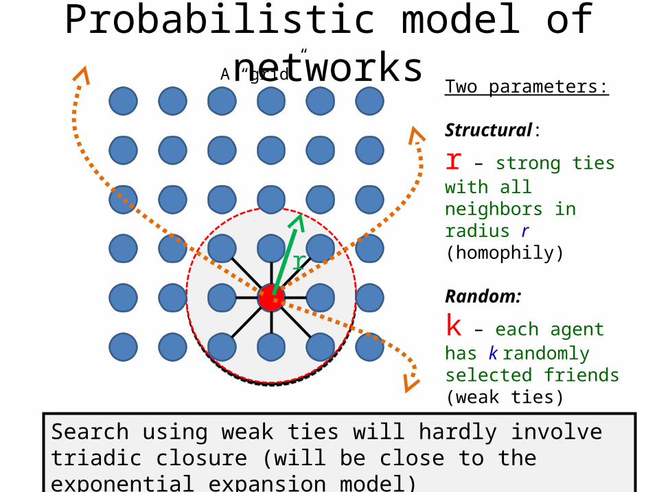
Two parameters:

Structural:

r – strong ties with all neighbors in radius r(homophily)

Random:

k – each agent has k randomly selected friends (weak ties)

r

Search using weak ties will hardly involve triadic closure (will be close to the exponential expansion model)

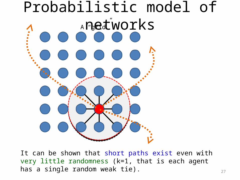
A “grid”

Probabilistic model of networks

27

It can be shown that short paths exist even with very little randomness (k=1, that is each agent has a single random weak tie).

A “grid”

The grid model

28

• Can the grid model we have just seen explain Milgram’s small world phenomenon?

• Problem: the choice of weak ties seems to be “too random”.

The grid model

29

(Taken from Milgram’s original paper)

Searching over the grid

30

• The agent has a message to deliver to a target person:– can only forward the message to his friends.– knows the location of the target on the grid.– knows only his own friends

• Neighbours (strong ties)• Random edges (weak ties)

• Important: the agent does not know the random edges of the others!

• A reasonable strategy: deliver to a friend which is closest/closer to the target.

• Problem: even when short paths exist, the delivery time might be long.

A modified model: Inverse Square

31

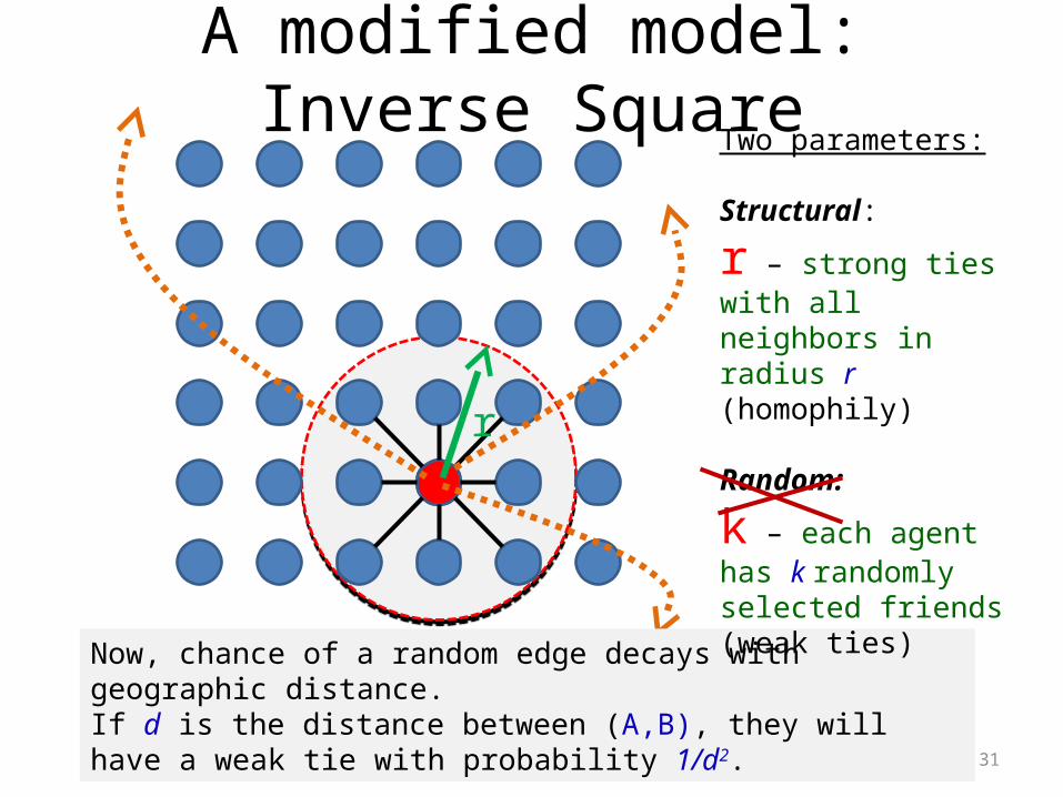
r

Now, chance of a random edge decays with geographic distance.If d is the distance between (A,B), they will have a weak tie with probability 1/d2.

Two parameters:

Structural:

r – strong ties with all neighbors in radius r(homophily)

Random:

k – each agent has k randomly selected friends (weak ties)

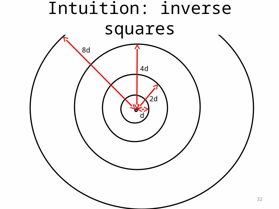
Intuition: inverse squares

32

d

2d

4d

8d

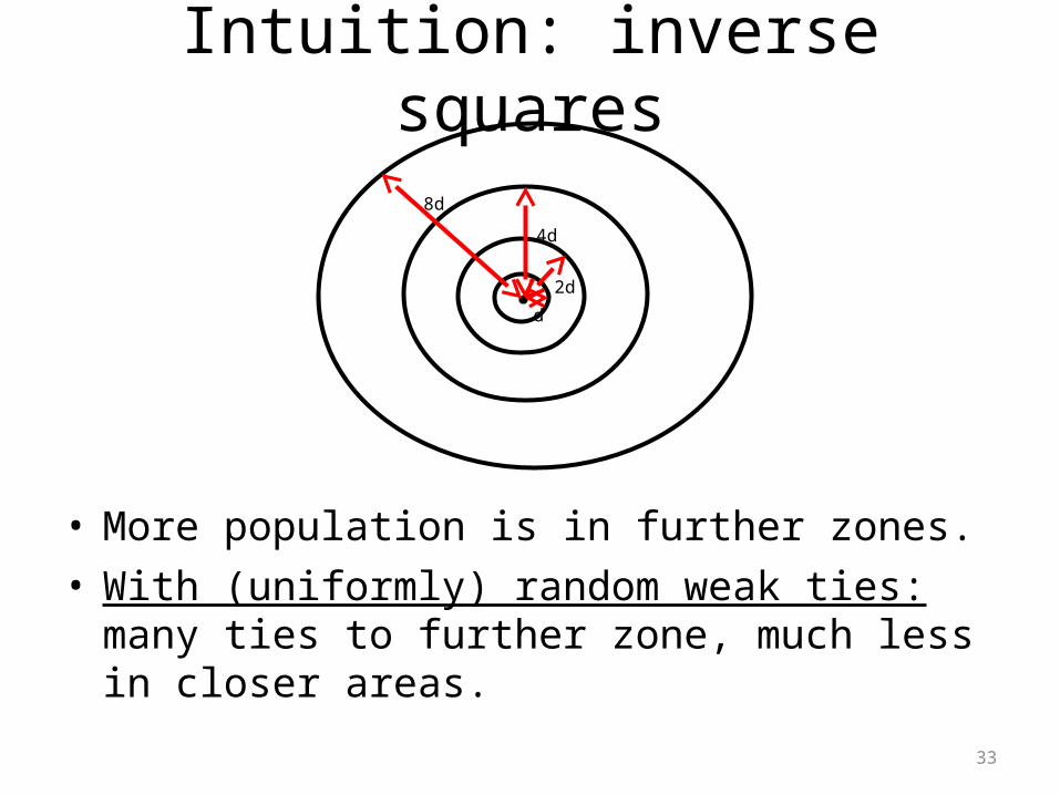
Intuition: inverse squares

33

d

2d

4d

8d

• More population is in further zones.• With (uniformly) random weak ties: many ties to

further zone, much less in closer areas.

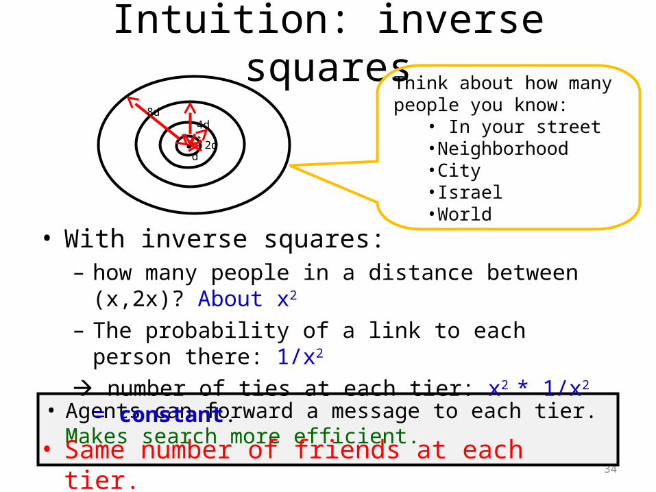
Intuition: inverse squares

34

d2d

4d8d

• Agents can forward a message to each tier. Makes search more efficient.

Think about how many people you know:

• In your street•Neighborhood•City•Israel•World

• With inverse squares:– how many people in a distance between (x,2x)? About x2

– The probability of a link to each person there: 1/x2

number of ties at each tier: x2 * 1/x2 = constant.

• Same number of friends at each tier.

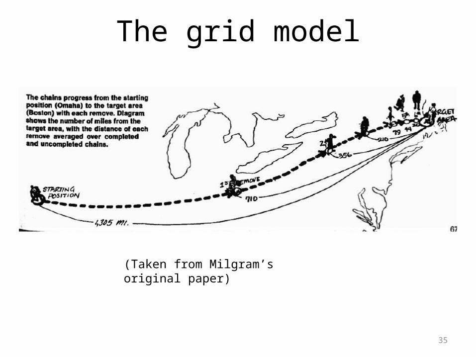
The grid model

35

(Taken from Milgram’s original paper)

The grid model

36

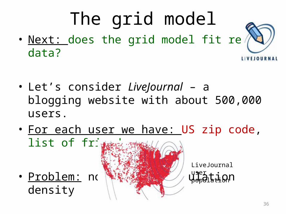
• Next: does the grid model fit real data?

• Let’s consider LiveJournal – a blogging website with about 500,000 users.

• For each user we have: US zip code, list of friends.

• Problem: non-uniform population density

LiveJournal user population

Distance by rank

37

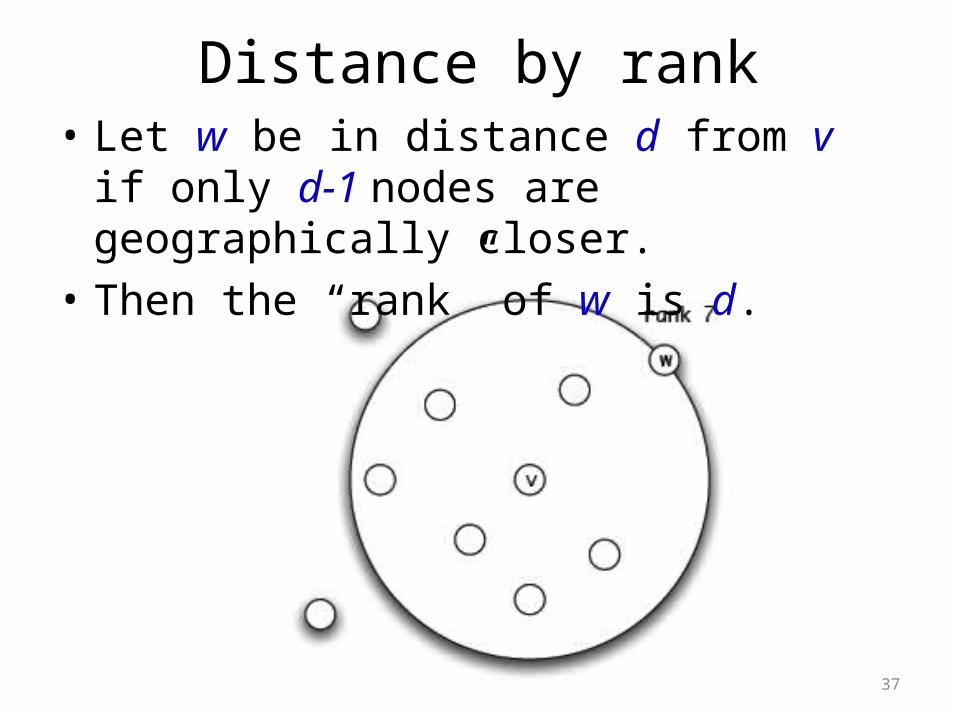
• Let w be in distance d from v if only d-1 nodes are geographically closer.

• Then the “rank” of w is d.

Distance by rank

38

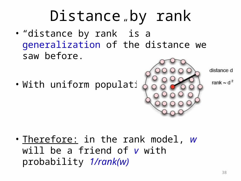
• “distance by rank” is a generalization of the distance we saw before.

• With uniform population:

• Therefore: in the rank model, w will be a friend of v with probability 1/rank(w)

Distance by rank

39

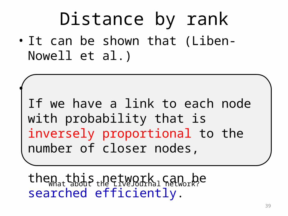
• It can be shown that (Liben-Nowell et al.)

•If we have a link to each node with probability that is inversely proportional to the number of closer nodes,

then this network can be searched efficiently.

What about the LiveJournal network?

Distance by rank

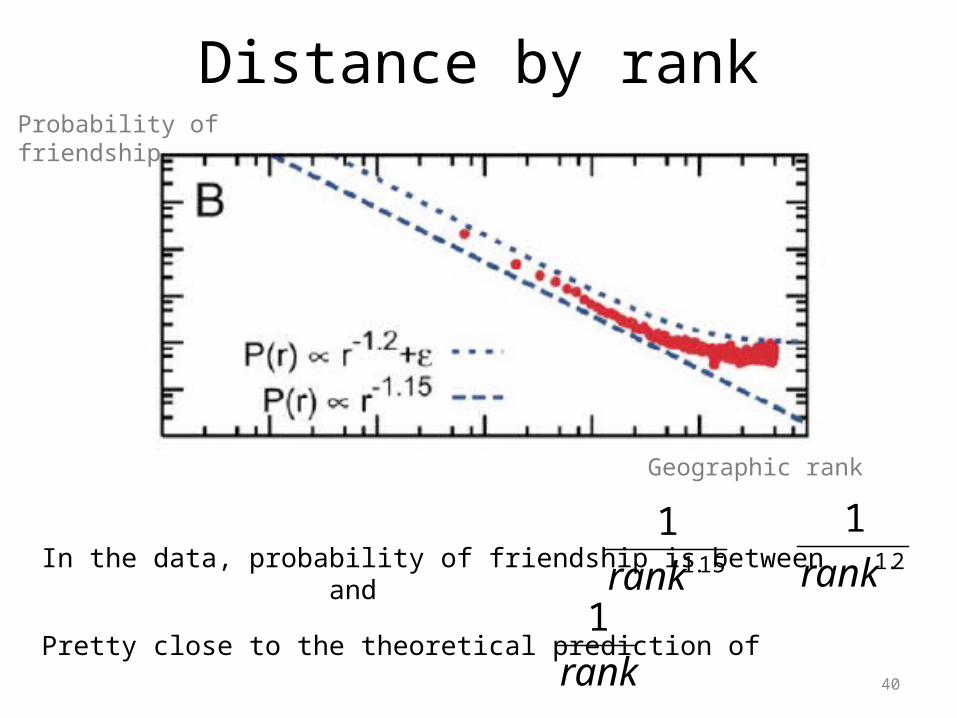
40

Probability of friendship

Geographic rank

In the data, probability of friendship is between and15.1

1

rank 2.1

1

rank

Pretty close to the theoretical prediction of rank

1

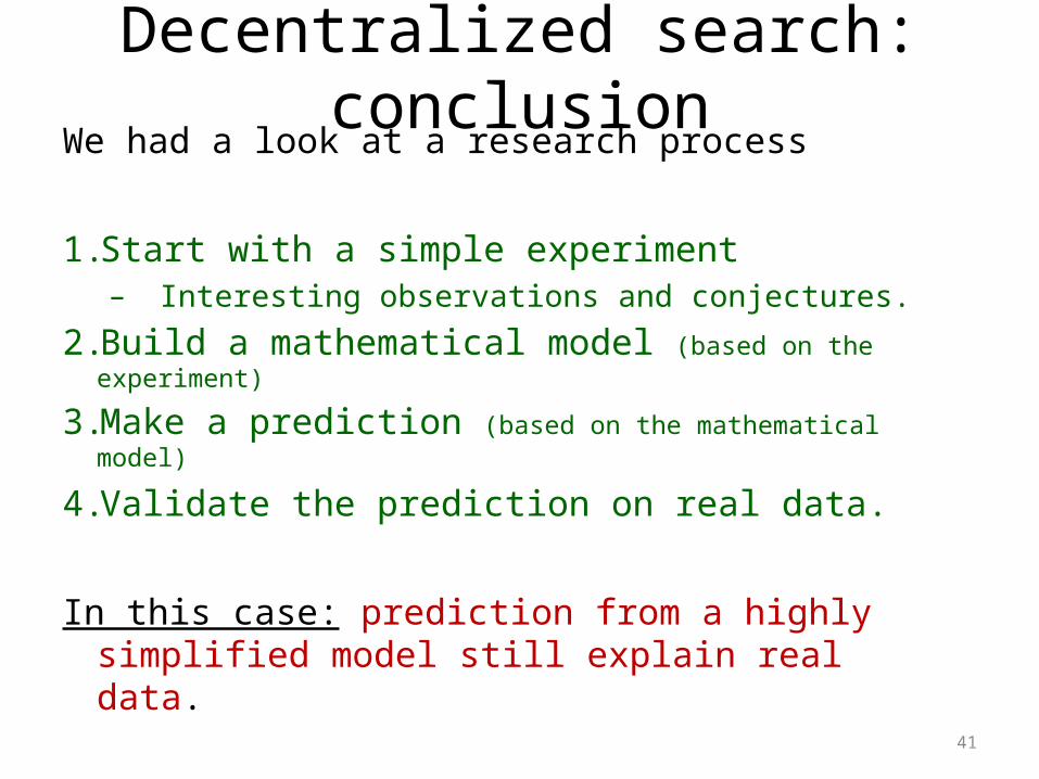
Decentralized search: conclusion

41

We had a look at a research process

1. Start with a simple experiment– Interesting observations and conjectures.

2. Build a mathematical model (based on the experiment)

3. Make a prediction (based on the mathematical model)

4. Validate the prediction on real data.

In this case: prediction from a highly simplified model still explain real data.

42

Some statistics for desert…

43

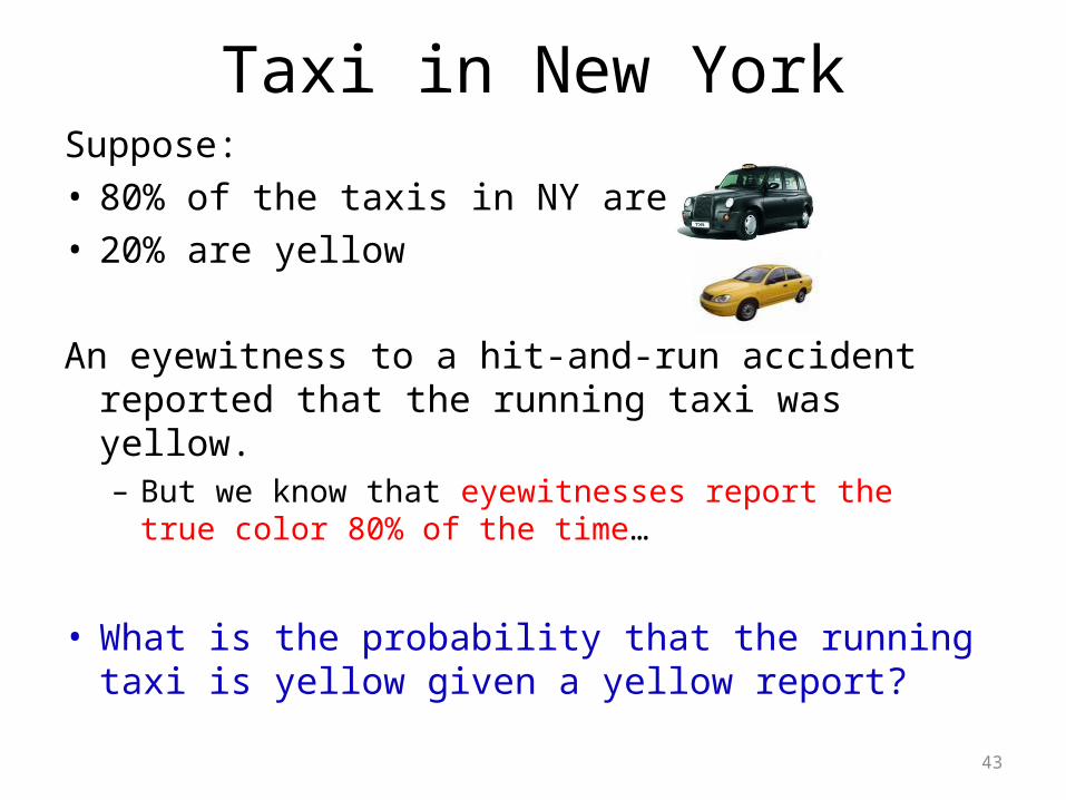
Suppose:• 80% of the taxis in NY are black• 20% are yellow

An eyewitness to a hit-and-run accident reported that the running taxi was yellow.– But we know that eyewitnesses report the true color 80%

of the time…

• What is the probability that the running taxi is yellow given a yellow report?

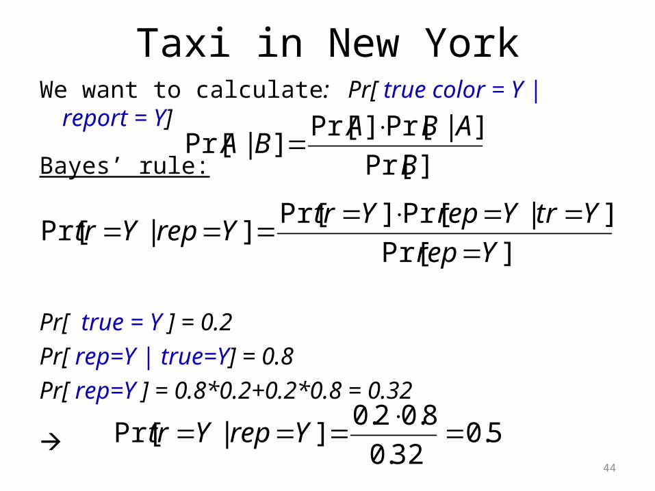
Taxi in New York

44

We want to calculate: Pr[ true color = Y | report = Y]

Bayes’ rule:

Pr[ true = Y ] = 0.2Pr[ rep=Y | true=Y] = 0.8Pr[ rep=Y ] = 0.8*0.2+0.2*0.8 = 0.32

Taxi in New York

]Pr[

]|Pr[]Pr[]|Pr[

B

ABABA

]Pr[

]|Pr[]Pr[]|Pr[

Yrep

YtrYrepYtrYrepYtr

5.032.0

8.02.0]|Pr[

YrepYtr

45

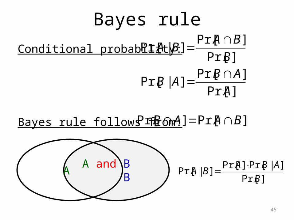
Conditional probability:

Bayes rule follows from:

Bayes rule

]Pr[

]Pr[]|Pr[

B

BABA

A and B B A

]Pr[

]Pr[]|Pr[

A

ABAB

]Pr[]Pr[ BAAB

]Pr[

]|Pr[]Pr[]|Pr[

B

ABABA

46

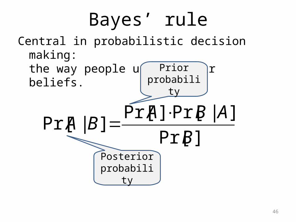
Central in probabilistic decision making:the way people update their beliefs.

Bayes’ rule

]Pr[

]|Pr[]Pr[]|Pr[

B

ABABA

Prior probability

Posterior probability

47

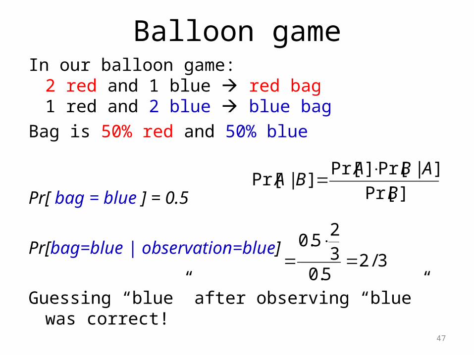
In our balloon game: 2 red and 1 blue red bag1 red and 2 blue blue bag

Bag is 50% red and 50% blue

Pr[ bag = blue ] = 0.5

Pr[bag=blue | observation=blue]

Guessing “blue” after observing “blue” was correct!

Balloon game

]Pr[

]|Pr[]Pr[]|Pr[

B

ABABA

3/25.032

5.0