Interplay between the gentlest ascent

dynamics method and conjugate directions to

locate transition states †

Josep Maria Bofill,∗,‡,¶ Jordi Ribas-Ariño,∗,§,¶ Rosendo Valero,∗,§,¶ Guillermo

Albareda,∗,§,¶,‖ Ibério de P.R. Moreira,∗,§,¶ and Wolfgang Quapp∗,⊥

Departament de Química Inorgànica i Orgànica, Secció de Química Orgànica and, Institut

de Química Teòrica i Computacional, (IQTCUB), Universitat de Barcelona, Martí i

Franquès 1, 08028 Barcelona, Spain , Departament de Ciència de Materials i Química

Física, Universitat de Barcelona, Martí i Franquès 1, 08028 Barcelona, Spain, Max Planck

Institute for the Structure and Dynamics of Matter and Center for Free-Electron Laser

Science, Luruper Chaussee 149, 22761 Hamburg, Germany, and Mathematisches Institut,

Universität Leipzig, PF 100920, D-04009 Leipzig, Germany

E-mail: jmbofill@ub.edu; j.ribas@ub.edu; valero@ub.edu; guillermo.albareda@mpsd.mpg.de;

i.moreira@ub.edu; quapp@uni-leipzig.de

Abstract†Dedicated to Professor Jean Paul Malrieu on occasion of his 80 birthday.∗To whom correspondence should be addressed‡Departament de Química Inorgànica i Orgànica, Secció de Química Orgànica and¶Institut de Química Teòrica i Computacional, (IQTCUB), Universitat de Barcelona, Martí i Franquès

1, 08028 Barcelona, Spain§Departament de Ciència de Materials i Química Física, Universitat de Barcelona, Martí i Franquès 1,

08028 Barcelona, Spain‖Max Planck Institute for the Structure and Dynamics of Matter and Center for Free-Electron Laser

Science, Luruper Chaussee 149, 22761 Hamburg, Germany⊥Mathematisches Institut, Universität Leipzig, PF 100920, D-04009 Leipzig, Germany

1

An algorithm to locate transition states on a Potential Energy Surface (PES) is

proposed and described. The technique is based on the Gentlest Ascent Dynamics

(GAD) method where the gradient of the PES is projected into a given direction and

also perpendicular to it. In the proposed method, named GAD-CD, the projection is not

only applied to the gradient but also to the Hessian matrix. Then the resulting Hessian

matrix is then block diagonal. The direction is updated according to the gentlest ascent

dynamics method. Furthermore, to ensure stability and to avoid high computational

cost, a trust region technique is incorporated and the Hessian matrix is updated at

each iteration. The performance of the algorithm in comparison with the standard

ascent dynamics is discussed for a simple two dimensional model PES. Its efficiency for

describing reaction mechanisms involving small and medium size molecular systems is

demonstrated for five molecular systems of interest.

1 Introduction

An extensive mathematical literature has been accumulated in the last fifty years for the

location of saddle points of index one on continuous and differentiable functions of several

variables. The interest for this type of points lies on the fact that they correspond to transi-

tion states (TS), which are the cornerstone of all chemical reaction rate theories and hence

are essential in establishing the mechanism of any chemical transformation. A saddle point

of index one is a stationary point on a surface and the corresponding Hessian matrix, the

matrix of second-order partial derivatives with respect to the coordinates, has one and only

one negative eigenvalue. Many different methods have been proposed in the literature that

are based on few common approximations thus, in many cases, it is difficult to establish

the effectiveness and differences among them. As it will be shown, the proposed Gentlest

Ascent Dynamics- Conjugate Directions (GAD-CD), method takes into account, in different

ways, the achievements and particularities of many previous methods to locate TSs. In this

way, we expect to have a robust and efficient method to locate such points. In contrast to

2

the original GAD method,1 we will demonstrate that GAD-CD allows for a second-order

expansion of the coordinates, thus making the method more robust.

The structure of the article is as follows. We will first provide in Section 2 a brief historical

review describing the nature of some of the most widely used methodologies for TS location

in order to put the proposed method in the appropriate context. We will then introduce

the mathematical basis of the GAD-CD method and also the flowchart of the associated

algorithm in Section 3. The performance and behavior is of the method is discussed and

analyzed in Section 4. Conclusions are given in Section 5.

2 Brief Historical Review of the Methods to locate Tran-

sition States

The most primitive method to locate TSs is the so-called grid search on a Potential Energy

Surface (PES).2,3 In this method the PES is evaluated on a spatial grid of points that is

assumed to span the saddle point of interest whose position is found by a polynomial fit.

The accuracy of the method depends on the resolution of the multi-dimensional grid, which

makes it prohibitive for moderate molecular systems.

Another widely used approach is the reaction coordinate method.4,5 Usually, in this

method one selects a specific internal coordinate -or a subset of them- as a reaction coordi-

nate. Step by step, the remaining coordinates are optimized between reactant and product

minima. The procedure can be seen as a predictor-corrector method. As a result one ob-

tains a reaction pathway and the corresponding energy profile where the maximum of which

would occur at the saddle point. A more recent generalization of the reaction coordinate is

the reduced gradient following (RGF) or Newton trajectory (NT).6–10 In this generalization

of the reaction coordinate the reaction pathway is built by the set of points such that the

3

gradient vector points to a constant direction. The curve passes through consecutive sta-

tionary points. In general, these methods involve a prediction of the selected variable and

optimization for the last N -1 variables taken as correctors, where N is the number of internal

coordinates. The optimization involves the calculation of the Hessian matrix in an exact or

approximated way. Note that different choices of the reaction coordinate, or what is the

same, a constant search direction of the gradient, produce different reaction pathways; some

of them have little or no chemical significance. Other types of reaction pathways have been

proposed like the following of a valley ground along a gradient extremal (GE).11–15 However,

their computational demand limits their applicability.

In the early years where the development of methods to locate TSs starts, the most com-

mon one was the minimization of the square of the gradient norm of the PES. This method

was originally proposed by McIver and Komornicki16,17 and consists in the minimization of

the function gT (x)g(x), where g(x) is the gradient vector at the point x of the PES function

V (x), i.e., gi(x) = ∂V (x)/∂xi for i = 1, . . . , N . It is used as a standard least square mini-

mization technique. Normally, the least squares algorithms show a poor rate of convergence.

The main disadvantage of these methods is that while the square of the gradient norm must

necessarily be zero at the TS, it is also zero at a local minimum or maximum of the PES

function and hence there may be other nonzero minima on the square of the gradient norm

surface for so-called shoulders. Thus, except in the case where one has an a-priori knowledge

of the PES and starts from a point sufficiently close to the position of the TS, there is no

guarantee that this method will converge to a TS. Nonetheless, a least squares minimization

algorithm has been proposed and applied to locate other types of points on the PES with

some degree of success.18

Other methods to locate TSs have been proposed to follow a reaction path from the

minimum of the PES uphill to the TS. These methods can be labeled as uphill walk. The

4

Crippen-Scheraga19 algorithm was the pioneer for climbing out of the minimum basin of

attraction. The method starts from the minimum point, xmin. At the iteration step i, the

system is translated along the pre-established direction d to yield xi = xmin + ρid where

ρi is a suitable step length. This is followed by an energy minimization on a hyperplane

perpendicular to d, HP i = {(x − xi)Td = 0}, to obtain xi+1 = arg minx∈HP i

V (x). The

iterative process is repeated until the system reaches a saddle point. More recently proposed

algorithms of this family for exploring high dimensional PES are based upon realizing that

evaluating the eigenmodes of the Hessian is central to the convergence to a TS.20 Another

algorithm was suggested by Cerjan and Miller.21 It requires the selection of a trust region

around a point on the multidimensional PES and it approximates the energy of the system

within this trust region by a quadratic expression. An optimal direction to translate the

system is then determined by evaluating the extremum of the energy on the boundary of

the trust region. The key for a reliable evaluation of the optimal direction relies in the

proper selection of the trust region. Within the same class of methods, Henkelman and

Jónsson22 proposed the dimer algorithm where the dimer consists of two points separated by

a small distance. The dimer moves towards the TS by a modification of the −g(x) vector,

namely, −g(x) + 2v(vTg(x)), where the direction v is the dimer direction being determined

by minimizing the dimer energy. Related to this type of methods, there is also the algorithm

proposed by Maeda et al.23 and Shang and Liu.24 More recently it has been proposed the so-

called Gentlest Ascent Dynamics (GAD)1 method that goes a step back and reformulates the

procedure of uphill walking through a set of ordinary differential equations whose solutions

converge to saddle points.25–30 The set of equations that governs the GAD is

dx

dt= −[I− 2vvT ]g(x), (1a)

dv

dt= −[I− vvT ]H(x)v, (1b)

where H(x) is the Hessian matrix, i.e., Hi,j(x) = ∂2V (x)/∂xi∂xj and t is the parameter

5

characterizing the GAD curve. Eq. (1a) means that the gradient is used by two different

components, one in the ascent direction of the v-vector subspace and the second in the de-

scent direction of the set of directions perpendicular to the v-vector. Eq. (1b) defines the

update of the ascent direction represented by the v-vector. The right hand side of Eq. (1b)

ensures that the v-vector converges to an eigenvector associated with the smallest eigenvalue

of H(x), and we have to make sure that the v-vector is normalized. At the starting point

the norm of the v(t0)-vector is equal to 1. We remark that the GAD algorithm can be

seen as a Zermelo-like navigation model on the PES to reach TSs in some optimal way, see

Refs. 29,30 for a demonstration. For this reason the v-vector is also called the control vector.

Another family of very important methods are known as quasi-Newton type. In these

methods the position of a local stationary point on the PES is located by an iterative proce-

dure briefly outlined as follows. At the i-th iteration, a direction ∆x(i) is calculated according

to the equation ∆x(i) = −H−1(i)g(i), where H−1(i) is an approximation to the inverse Hessian

matrix and g(i) is the gradient vector at the point x(i). The Hessian matrix is computed at the

first iteration and subsequently updated during the procedure. The various quasi-Newton

methods differ in the way in which the Hessian matrix (or its inverse) is updated. The

new estimate of the stationary point x(i+1) is usually taken as x(i+1) = x(i) + ∆x(i).31 There

may seem to be no reason why this type of methods, just outlined, could not be used for

locating TSs, so long as at each iteration the Hessian matrix has one and only one negative

eigenvalue. A quasi-Newton like method was devised by Schlegel for the first time.32,33 The

quasi-Newton methods, however, suffer from the disadvantage that there is no way to pre-

venting the Hessian matrix from becoming positive definite, which would cause the method

to locate a local minimum rather than a TS. We note that quasi-Newton methods to find

TSs can be seen as uphill walk methods from a minimum towards a saddle point of index

one, achieved by maximizing the quadratic approximation of the PES along a direction and

minimizing it along the other directions. The problem to avoid a positive Hessian matrix in

6

the quasi-Newton search of TSs was considered by Banerjee et al.34,35 and others.36–39 This

is achieved using the Levenberg-Marquardt technique31 consisting of a parametric modifica-

tion of the second order term in the quadratic expansion, such that the resulting “perturbed”

Hessian matrix has a negative eigenvalue in one direction and positive eigenvalues in the re-

maining directions.

The first algorithm proposed for locating TSs based on the conjugate gradient optimiza-

tion method was due to Sinclair and Fletcher.40 This type of methods allows for the use of

line searches without the generation of search directions of zero curvature. The basic concept

of these methods is the so-called conjugacy. Let us assume an N -dimensional quadratic PES

with Hessian matrix H. Then we say that two vectors, v(i) and v(j), are H-conjugate when

they have the property that v(i)THv(j) = 0.31 If the Hessian matrix has only one negative

eigenvalue and if the v(i)-vector is a direction of negative curvature, i.e. v(i)THv(i) < 0,

then the remaining conjugate vectors, v(j) (j 6= i), have necessarily non-negative curvature.

Briefly, the structure of these methods to locate a TS is described as follows. We start at

a point x(1), assumed to be in the midpoint between two minima, and with a v(1)-vector

which depicts the straight line joining these minima. The first iteration consists in searching

the maximum x(2) along the line v(1). A conjugate vector, v(2), is then computed as the

component of −g(2), H-conjugate to v(1), resulting in

v(2) = −g(2) +g(2)T (g(2) − g(1))

v(1)T (g(2) − g(1))v(1) = −g(2) + (g(2)Th(1))v(1) . (2)

Thus, the v(2) conjugate vector is found only using the gradients g(1) and g(2), and the orig-

inal vector v(1). A search for a minimum is made along this new vector. In a similar way in

the subsequent iterations new H-conjugate vectors are generated, say v(i+1), using only the

gradient g(i+1), the vectors h(1), v(1) and v(i). The new H-conjugate vectors are obtained

through the expression v(i+1) = −g(i+1) + (g(i+1)Th(1))v(1) + ||g(i+1)||/||g(i)||v(i), and linear

7

searches are in turn carried out along each of these directions. After each iteration, it is

necessary to make a test to ensure that the current gradient along the initial vector, v(1),

is still close to zero. If the current gradient, g(i+1), along the v(1)-vector is too large then

the algorithm is restarted by replacing x(1) with the current point, x(i+1). The algorithm

continues until the gradient norm is less than a given tolerance. We note that if the exact line

searches are performed on a quadratic function then the magnitude v(1)Tg(i) would remain

zero throughout. Also, the algorithm would never need to restart. In other words, using

this method on a quadratic PES the TS would be found in at most N iterations, being N

the number of variables. On the other hand, on a non-quadratic PES it is always neces-

sary to check the projection of the current gradient along the v(1)-vector to ensure that the

algorithm converges to the TS. The main disadvantage of these methods is that the conver-

gence rate is rarely well behaved. Even on a quadratic PES there is no guarantee that a

conjugate gradient method will converge in N iterations, whereas the quasi-Newton method

will converge in one iteration given the exact Hessian matrix. It is, in fact, well known that

the quasi-Newton methods will converge to stationary points much faster than any general

conjugate direction methods, in particular the conjugate gradient.

It is worth mentioning the algorithm proposed by Bell et al.41,42 that works well on PESs

that are not far from quadratic. This algorithm commences, as above, by finding a maximum

along a v(1)-vector that is known to have negative curvature. Furthermore, a quasi-Newton

minimization is then made in a space of (N − 1) linearly independent vectors which is H-

conjugate to the v(1)-vector. If the PES is quadratic then the gradient component along

this vector would remain zero during the minimization in the (N − 1)-space H-conjugate to

the v(1)-vector. In non-quadratic PESs this gradient could be different from zero. For this

reason, conjugate gradient methods require a test to check the value of this gradient and, if

necessary, another search along the v(1) vector for a maximum. Thereafter a new minimiza-

tion on the (N − 1)−H-conjugate space is carried out. This ensures that the algorithm is

8

stable and converges to a TS. We note that the algorithm of Bell et al.41,42 is based on an

interplay between conjugate gradient and quasi-Newton methods. The conjugate gradient

performs the maximization whereas the quasi-Newton method performs the minimization to

find the TS. The main difficulty of this algorithm appears when the TS is very far from the

line characterized by the v(1)-vector and frequently the H matrix ceases to have negative

curvature after some minimizations. These difficulties were partially solved in a later im-

provement of the method.42

The so-called synchronous transit method proposed by Halgren and Lipscomb43 has in-

spired a large number of algorithms. The synchronous transit methods consist, like the

conjugate gradient method, in alternating maximum and minimum searches, starting with

a search for a maximum along the line joining two known minima of the PES, the linear

synchronous transit. A minimization is then carried out along directions orthogonal to the

linear synchronous transit followed by a maximum search of a parabolic path containing the

two minima and the current estimate of the TS. This minimization and maximization search

process is repeated until the TS is reached. Schlegel et al.44 improved the original algorithm

of Halgren and Lipscomb43 by doing a combination of synchronous transit and quasi-Newton

minimizations. Other algorithms that can be classified within this set of methods are those

given in the Refs. 45–51. It is worth to mention a recent improvement within this type of

methods due to Zimmerman.52

The algorithm presented in this work, the GAD-CD method, is designed as an inter-

play between the conjugate direction,31,53 quasi-Newton31 and GAD methods.1 In part, the

algorithm is based on the results from Bell et al.,41 GAD1 and also the restricted step tech-

nique31 to improve the stability of the entire procedure to locate TSs on general PESs. In the

following section we explain and summarize the basic mathematical points of the algorithm

and its implementation.

9

3 The GAD-CD Method

3.1 The Mathematical Basis

We will find a stationary point say, xTS, on a PES, V (x), by successive quadratic expansions

of this surface, denoted by q(x). The dimension of the x vector is N . Let v1 be a given

normalized direction vector such that the energy increases in this direction. Let x0 be a

point where the quadratic expansion is centered and q(x0 + v1a1) is maximized over a1.

We expect to construct a VN−1 matrix of dimension N × (N − 1) with N − 1 independent

column vectors, VN−1 = [v2| . . . |vN ], such that VTN−1H0v1 = 0N−1, where H0 is the Hessian

matrix at x0 and 0N−1 the zero vector of dimension N − 1. Under this condition we can say

that the direction x′ − x0 = VN−1aN−1 is H0-conjugate to the v1 direction vector, where

aN−1 = (a2, . . . , aN)T , is a vector of dimension N − 1 and it is different from the zero vector.

More specifically, (x′−x0)TH0v1 = aTN−1V

TN−1H0v1 = aTN−10N−1 = 0, which is the conjugacy

condition. Then, from the theory of conjugate directions it can be shown that the matrix

V = [v1|VN−1] is non-singular and hence that VTH0V can be chosen in such a way that the

resulting matrix has a negative curvature on vT1 H0v1 and VTN−1H0VN−1 is positive definite.

In this way q(x0 +VN−1aN−1) = V (x0) + gT0 VN−1aN−1 + 1/2aTN−1VTN−1H0VN−1aN−1 has a

unique minimizing point

x′ = x0 −VN−1(VTN−1H0VN−1)

−1VTN−1g0 (3)

where g0 is the gradient of the PES at x0. If g(x′), the gradient of the PES at x′, satisfies

thatVTg(x′) = 0, then x′ is a saddle point of index one or a TS on q(x′) and also on the PES.

Now the task to write an algorithm is reduced firstly to find a suitable VN−1 matrix and

secondly to search a way to find the v1 direction vector. TheVN−1 matrix can be constructed

and obtained from an elementary Householder orthogonal matrix Q = I− 2w(wTw)−1wT ,

10

where w is a vector of dimension N such that Qt = ±||t||e1, and t = H0v1, e1 is the

first column of the unit matrix I of dimension N × N and ||t|| = (tT t)1/2.41 Thus the

symmetric orthogonal matrix Q = [q1|QN−1] constructed in this way is such that tTQ =

vT1 H0Q = (vT1 H0q1,vT1 H0QN−1) = (vT1 H0q1,0

TN−1) = (±||t||,0TN−1) = ±||t||eT1 . QN−1 is

then an N × (N − 1) matrix of independent columns satisfying QTN−1H0v1 = 0N−1 and thus

a representation of the VN−1 matrix, QN−1 = VN−1. The Q matrix is a rank-one matrix

with the unit matrix I

Qt = (I− 2w(wTw)−1wT )t = ±||t||e1 . (4)

If we take 2(wTw)−1wT t = 1, then the vector w = t± ||t||e1 and 2(wTw)−1 = (wT t)−1 =

(tT t± ||t||t1)−1 where t1 is the first component of the t vector. The resulting matrix Q is

Q = I− 2w(wTw)−1wT = I− (t± ||t||e1)(tT t± ||t||t1)−1(t± ||t||e1)T . (5)

The last N − 1 columns of this matrix form the QN−1 matrix, V = [v1|VN−1] = [v1|QN−1].

We note that the idea underlying the above results is a theorem due to Powell on the parallel

subspace property of conjugate directions.31,53 This theorem establishes that on a quadratic

surface, for a1 6= 0 the relation ∆g0 = g(x0 + v1a1) − g(x0) = H0v1a1 always holds. If the

gradient difference vector ,∆g0, has a null projection into the subspace spanned by the set of

linear independent vectors, VN−1, then these vectors are H0-conjugate with respect to the

vector v1. In other words, VTN−1∆g0 = VT

N−1H0v1a1 = 0N−1 implies the H0-conjugacy since

by hypothesis a1 6= 0. Notice that the set of vectors, VN−1, can be H0-conjugate within

them or not, the only requirement is their linear independence. This theorem permits us to

propose an extension until quadratic order in ∆x of the GAD method, by minimizing the

energy surface in the subspace spanned by the set of vectors H0-orthogonal to the direction

of the control vector v1. Now, we only need a correction to the second order expansion and

the way to update the v1-vector. As will be shown below the first question is addressed

11

through the restricted step technique.31

The quadratic approximation of the PES, V (x), around x0 takes the form

V (x0 + ∆x0) ≈ q(x0 + ∆x0) = q(x0 + Va) = V (x0) + aTVTg0 + 1/2aTVTH0Va =

V (x0) + a1vT1 g0 + 1/2a21v

T1 H0v1 + aTN−1V

TN−1g0 + 1/2aTN−1V

TN−1H0VN−1aN−1 =

V (x0) + q+(a1) + q−(aN−1)

(6)

where ∆x0 = x−x0, aT = (a1, aTN−1) and ∆x0 = Va. The confidence in the quadratic approx-

imation is warranted by a restricted step method characterized by a trust radius r defined as

aTa = ||a||2 ≤ r2. The TS search is performed via a maximization of the quadratic approxi-

mation q+(a1) along the subspace v1, and a minimization of the approximation q−(aN−1) in

the VN−1 subspace. Both subspaces are H0-conjugate, since VTN−1H0v1 = 0N−1.

The mathematical formalization of the above problem can be written as

qoptimal(x0 + Va) = V (x0) + Maxa1 MinaN−1{q+(a1) + q−(aN−1) | aTa ≤ r2 and a ∈ RN} =

V (x0) + Mina{−q+(a1) + q−(aN−1) | aTa ≤ r2 and a ∈ RN}(7)

where r is a positive scalar. A solution of this problem can be found using the Lagrangian

multipliers method

L(a, λ) = −q+(a1) + q−(aN−1) + λ/2(aTa− r2) . (8)

Differentiation with respect to a and λ yields, after some rearrangements, the equations

a = −(M0 + λI)−1h0 , (9a)

aTa− r2 = 0 (9b)

12

where hT0 = (−gT0 v1,gT0 VN−1) and M0 is the block diagonal matrix,

M0 =

−vT1 H0v1 0TN−1

0N−1 VTN−1H0VN−1

(10)

of dimension N ×N . Substituting Eq. (9a) into Eq. (9b), we obtain the secular function

f(λ) = hT0 (M0 + λI)−2h0 − r2 (11)

the zeros of which are to be computed. To solve the Max-Min problem, the parameter λ is

chosen to satisfy f(λ) = 0 and the two conditions:

1. (vT1 H0v1−λ) < 0 to obtain an uphill direction of q(x) in the subspace spanned by v1,

2. det(VTN−1H0VN−1+λIN−1) > 0 to obtain an downhill direction of q(x) in the subspace

spanned by the set of columns of VN−1.

Here IN−1 is the unit matrix of dimension (N − 1) × (N − 1). If the H0 has the expected

structure and the quasi-Newton step lies within the boundary of the trust region, aTa < r2,

then the quasi-Newton step is taken. Otherwise the step is chosen in the boundary of the

trust region, aTa = r2, by finding the λ that satisfies f(λ) = 0 and the above conditions 1

and 2.

Now we propose an algorithm that solves the secular function f(λ) = 0 of Eq. (11). To

this end we multiply this equality by the quantity, hT0 br−2, where b is a vector different

from zero of dimension N and not orthogonal to the h0 vector. The resulting expression is

hT0 [b− (M0 + λI)−2h0hT0 br

−2] = 0 . (12)

Since h0 6= 0 then we can write, (M0 + λI)2b − h0hT0 br

−2 = 0. By defining a new vector,

p = (M0 +λI)b, the latter equation can be written in the form (M0 +λI)p−h0hT0 br

−2 = 0.

13

The above two equalities can be written in a compact form as an eigenvalue equation

−M0 I

r−2h0hT0 −M0

b

p

= λ

b

p

. (13)

Let us denote the real solutions of this real nonsymetric eigenvalue Eq. (13) by the triples,

{(λi,bTi ,pTi )}nreali=1 , where λi are given in increasing order and nreal ≤ 2N . Substituting any

real triple in the eigenvalue Eq. (13) and using Eq. (9a) we obtain,

ai = −pi(hT0 bi)−1r2 i = 1, . . . , nreal . (14)

If we multiply Eq. (14) from the left by −hT0 (M0+λI)−1 and if we take into account Eq. (9a)

and the fact that hT0 (M0 + λI)−1pi = hT0 bi, then we conclude from Eq. (13) that all these

solutions satisfy the relation aTi ai = r2 for i = 1, . . . , nreal. Within these real solutions we

have to find the solution that satisfies the above considerations 1 and 2. It is easy to check

that the triple solution whose λi is located in the interval, ]max{vT1 H0v1,−hmin, 0},+∞[,

where hmin is the lowest eigenvalue of VTN−1H0VN−1, satisfies these two requirements. We

take the triple whose λi has the lowest value in the interval, that it is (λ1,bT1 ,p

T1 ) corre-

sponding to the tuple (λ1, aT1 ), through Eq. (14). The selected tuple, (λ1, a

T1 ), is called from

now, (λ, aT ). We emphasize that this tuple is the solution of Eqs. (9) and in addition satisfies

the conditions 1 and 2. With this choice qoptimal(x + Va) has the minimum value because λ

is the lowest eigenvalue. Note that

qoptimal(x + Va)− V (x0) = 1/2(aT I−h0 − λaT I−a) = 1/2(aT I−h0 + λ(2a21 − r2)) (15)

where

I− =

−1 0TN−1

0N−1 IN−1

, (16)

14

and a1 is the first component of the a vector. In the derivation of Eq. (15) we have used

the equality, r2 = aTa = a21 + aTN−1aN−1, where, aN−1 = (a2, . . . , aN)T . The trust radius is

updated according to the following simple algorithm. First, the new V (x) is computed where

x = x0 + ∆x0 = x0 + Va obtained from the tuple with λ. Second, we compute the quotient

c = (V (x)− V (x0))/(qoptimal(x0 +Va)− V (x0)). Now, if c ≤ cmin or c ≥ (2− cmin), then we

set r/cf → r. Contrarily, if c ≥ caccep and c ≤ (2− caccep) and aTa < r2, then a is evaluated

according to a pure Newton step, that is, if a = −M−10 h0, then rc

1/2f → r. Throughout we

take cmin = 0.75, caccep = 0.80 and cf = 2. The displacement ∆x0 is accepted if 0 < c < 2.

Otherwise a new set of triples is computed with the new r but the same x0 and a new c is

obtained and tested. This is repeated until 0 < c < 2.

If for the new x, ||g(x)|| is lower than a threshold, then the process has converged and x

is a TS. Otherwise we first update the v1 vector, the control vector, according to the second

GAD formula, Eq. (1b)

v′1 = s[v1 −m(I− v1vT1 )H0v1] (17)

where s is the normalization factor such that v′T1 v′1 = 1 and m = (∆xT0 ∆x0)

1/2. Second

with the new gradient g(x) the vector j0 = g(x)− g(x0)−H0∆x0 is built and the Hessian

matrix is updated according to the general Greenstadt variational formula54

H = H0 + j0uT0 + u0j

T0 − (jT0 ∆x0)u0u

T0 (18)

where u0 = W∆x0/(∆xT0W∆x0), being W the inverse of a symmetric positive weighted

matrix. In order to use the Murtagh-Sargent-Powell update formula, in the present algo-

rithm we take W = φ∆x0∆xT0 + (1 − φ)j0jT0 where φ = (jT0 ∆x0)

2(∆xT0 ∆x0jT0 j0)

−1.31,54–59

Notice that uT0 ∆x0 = 1 and thus the condition, H∆x0 = g(x)− g(x0), is satisfied. Finally,

we reveal the potential energy, vectors and matrices, V (x)→ V (x0), x→ x0, g(x)→ g(x0),

v′1 → v1 and H→ H0 and a new iteration begins constructing the Q matrix, Eq. (5), and

15

solving the problem given in Eq. (7).

As a final comment, we remark some basic equivalences between the GAD algorithm1,25–30

and the GAD-CD presented in this work. In the original GAD model, the trajectory opti-

mally transverses the set of equipotential surfaces while evolving towards the TS, see Eq.

(17) in reference 30. The trajectory is guided by the v-vector. Alternatively, in the GAD-CD

method, each point of the trajectory satisfies an optimal Max-Min solution of a quadratic

approximation to the PES, see Eq. (7). This optimal solution does also depend on the

v1-vector. In both methods the v-vector is found at each point under the condition that

it minimizes the Rayleigh-Ritz quotient, vT1 H0v1/(vT1 v1), given in Eq. (1b) for the GAD

method and Eq. (17) for the GAD-CD.

3.2 Description of the Algorithm

The above detailed GAD-CD method can be practically implemented according to an op-

erational algorithm that can be schematically described according to the flowchart below.

The sub-index, i, and the super-index, (i), refer to the iteration number. This algorithm has

been interfaced with the Turbomole package.60

1. Initialization

(a) Choose a guess x0 and an initial trust radius r0.

(b) Calculate the potential energy, V0, the gradient vector, g0, and the Hessian matrix,

H0.

(c) Select the normalized v(0)1 -vector, usually an eigenvector of the H0 matrix.

(d) Set i = 0.

2. Hessian and gradient transformation

(a) Compute the element v(i)T1 Hiv

(i)1 .

16

(b) Evaluate the vector w(i) = t(i)− ||t(i)||e1 where t(i) = Hiv(i)1 , and hence calculate

Q(i) according to Eq. (5). Obtain the V(i)N−1 matrix from Q(i) by taking the last

N − 1 columns.

(c) Calculate V(i)TN−1HiV

(i)N−1 and hi = [−v(i)

1 |V(i)N−1]

Tgi.

(d) Build the Mi-matrix according to Eq. (10) taking into account that v(i)T1 Hiv

(i)1

should be multiplied by −1, v(i)T1 Hiv

(i)1 → −v

(i)T1 Hiv

(i)1 .

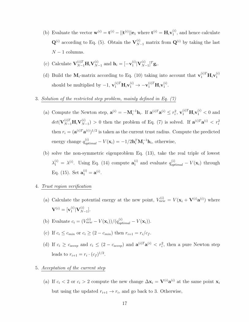
3. Solution of the restricted step problem, mainly defined in Eq. (7)

(a) Compute the Newton step, a(i) = −M−1i hi. If a(i)Ta(i) ≤ r2i , v

(i)T1 Hiv

(i)1 < 0 and

det(V(i)TN−1HiV

(i)N−1) > 0 then the problem of Eq. (7) is solved. If a(i)Ta(i) < r2i

then ri = (a(i)Ta(i))1/2 is taken as the current trust radius. Compute the predicted

energy change q(i)optimal − V (xi) = −1/2hTi M−1i hi, otherwise,

(b) solve the non-symmetric eigenproblem Eq. (13), take the real triple of lowest

λ(i)1 = λ(i). Using Eq. (14) compute a

(i)1 and evaluate q(i)optimal − V (xi) through

Eq. (15). Set a(i)1 = a(i).

4. Trust region verification

(a) Calculate the potential energy at the new point, V (i)new = V (xi + V(i)a(i)) where

V(i) = [v(i)1 |V

(i)N−1].

(b) Evaluate ci = (V(i)new − V (xi))/(q

(i)optimal − V (xi)).

(c) If ci ≤ cmin or ci ≥ (2− cmin) then ri+1 = ri/cf .

(d) If ci ≥ caccep and ci ≤ (2 − caccep) and a(i)Ta(i) < r2i , then a pure Newton step

leads to ri+1 = ri · (cf )1/2.

5. Acceptation of the current step

(a) If ci < 2 or ci > 2 compute the new change ∆xi = V(i)a(i) at the same point xi

but using the updated ri+1 → ri, and go back to 3. Otherwise,

17

(b) check the convergence criteria on {|(∆xi)µ|}Nµ=1 ≤ εx and {|(gi)µ|}Nµ=1 ≤ εg. If

they are fulfilled, the process has converged and the point xi is the first-order

saddle point. Otherwise,

(c) make xi+1 = xi + ∆xi, V(i)new = V (xi+1), and compute g(xi+1) = gi+1. Using

Eq. (17) to update the v1 and set v(i+1)1 to the new vector. Finally update the

approximate Hessian matrix using Eq. (18). Set i = i+ 1 and go back to 2.

4 Applications and Performance of the GAD-CD Algo-

rithm

4.1 Comparison between GAD and GAD-CD Algorithms

The performance of the GAD-CD algorithm has been tested and compared with results

obtained using the GAD algorithm on the Müller-Brown PES61 a simple two-variable model

PES. The behavior of both methods is shown in Fig.(1). In both cases we consider the

starting point, (−0.7, 1.2), located near to the minimum of the deep valley of the PES. The

initial v-vectors are in each case the eigenvector corresponding to the lowest eigenvalue, v1,

and the highest eigenvalue, v2, of the Hessian matrix evaluated at this initial point. The

components of these two vectors are v1 = (0.651, 0.759) and v2 = (0.759,−0.651). The TS

achieved by both methods is that located at the point (−0.822, 0.624). The integration of

the GAD equations, Eqs. (1), is carried out using the Runge-Kutta-4,5 with adaptive size

control and the Cash-Karp parameters.62 The Hessian matrix was computed analytically at

each step of integration as required by the second GAD equation, namely, Eq. (1b). The

step size of integration was taken very small, h = 1 · 10−6, otherwise the algorithm does not

converge. The reason of this small step size is due to the fact that the initial point is located

in a very deep valley. When the initial control vector is v1 the GAD does not reach the

transition state. The curve evolves toward the Müller-Brown plateau region, see Fig. (1a).

18

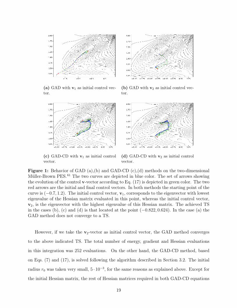
(a) GAD with v1 as initial control vec-tor.

(b) GAD with v2 as initial control vec-tor.

(c) GAD-CD with v1 as initial controlvector.

(d) GAD-CD with v2 as initial controlvector.

Figure 1: Behavior of GAD (a),(b) and GAD-CD (c),(d) methods on the two-dimensionalMüller-Brown PES.61 The two curves are depicted in blue color. The set of arrows showingthe evolution of the control v-vector according to Eq. (17) is depicted in green color. The twored arrows are the initial and final control vectors. In both methods the starting point of thecurve is (−0.7, 1.2). The initial control vector, v1, corresponds to the eigenvector with lowesteigenvalue of the Hessian matrix evaluated in this point, whereas the initial control vector,v2, is the eigenvector with the highest eigenvalue of this Hessian matrix. The achieved TSin the cases (b), (c) and (d) is that located at the point (−0.822, 0.624). In the case (a) theGAD method does not converge to a TS.

However, if we take the v2-vector as initial control vector, the GAD method converges

to the above indicated TS. The total number of energy, gradient and Hessian evaluations

in this integration was 252 evaluations. On the other hand, the GAD-CD method, based

on Eqs. (7) and (17), is solved following the algorithm described in Section 3.2. The initial

radius r0 was taken very small, 5 · 10−3, for the same reasons as explained above. Except for

the initial Hessian matrix, the rest of Hessian matrices required in both GAD-CD equations

19

at each step of the process is updated according to the formula given in Eq. (18). The total

number of energy and gradient calculations needed for the GAD-CD to reach the TS was 154

when the starting control vector is v1-vector and 150 when the initial vector is v2. We recall

that, in contrast to the GAD method, only the initial Hessian was evaluated analytically

and updated during the process. This two-dimensional example shows the efficiency of

the GAD-CD method compared to the GAD method. Using an update rather than the

analytic Hessian matrix, the GAD-CD reaches the TS with a lower number of energy and

gradient calls than the GAD method. Furthermore, the GAD-CD method converges to the

TS independently of the initial control vector. Notice that both curves do not evolve in the

same way in what the evolution of the control vector is concerned.

The different behavior of GAD and GAD-CD methods is due to different type of optimiza-

tion in their evolution. Whereas GAD evolves satisfying an optimal transversality,29,30 the

GAD-CD evolves solving the optimization of both Eq. (7) and the Rayleigh-Ritz quotient,

vTHv/(vTv), through Eq. (17).

In terms of computational efficiency, robustness and stability, the GAD-CD algorithm is

superior to GAD with a lower time step. In addition GAD-CD shows low dependence on the

guess structure and the control vector to reach the transition state. Notice that the search

starts far from the TS and very close to the deep minimum.

4.2 Behavior on Molecular Systems

The GAD-CD algorithm was interfaced with the Turbomole package60 in order to assess

its performance in molecular systems. Five different reactions were employed to test the

performance of the GAD-CD algorithm:

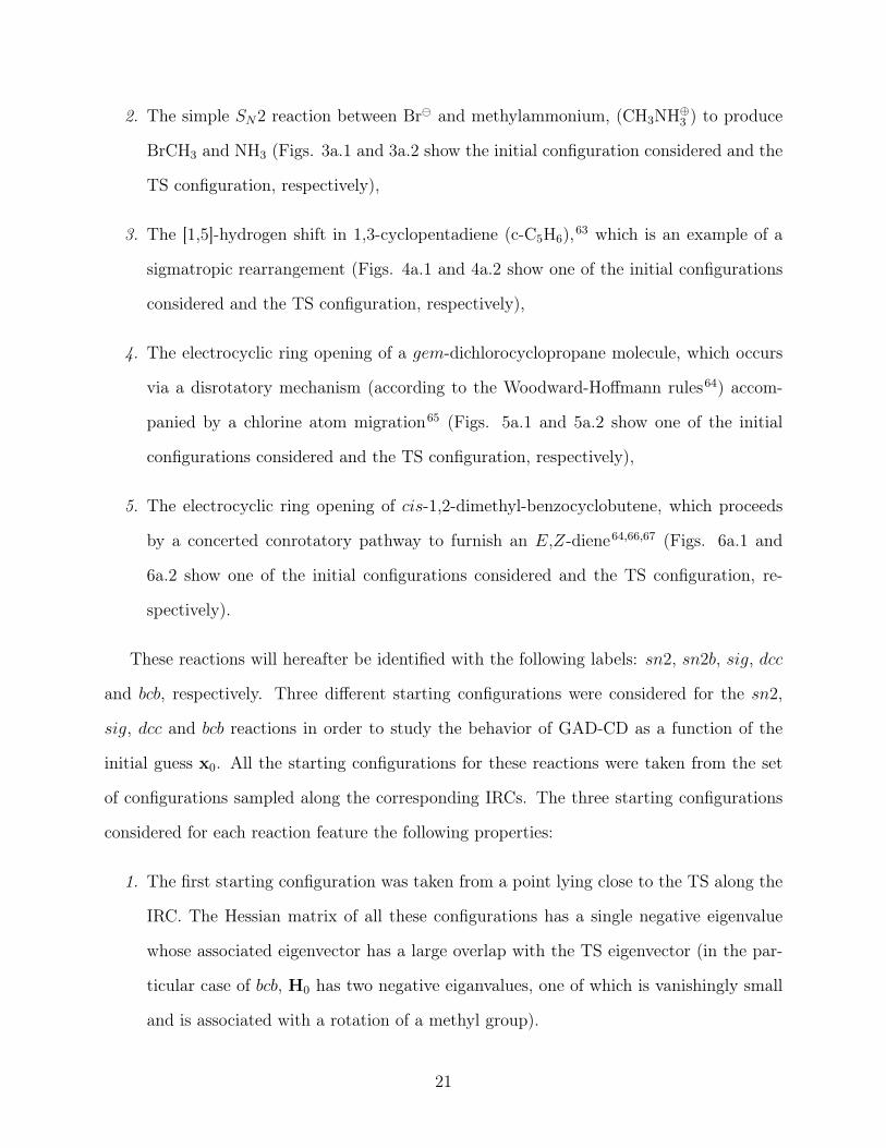
1. The simple SN2 reaction between Cl and CH3F to produce F and CH3Cl (Figs. 2a.1

and 2a.2 show one of the initial configurations considered and the TS configuration,

respectively),

20

2. The simple SN2 reaction between Br and methylammonium, (CH3NH⊕3 ) to produce

BrCH3 and NH3 (Figs. 3a.1 and 3a.2 show the initial configuration considered and the

TS configuration, respectively),

3. The [1,5]-hydrogen shift in 1,3-cyclopentadiene (c-C5H6),63 which is an example of a

sigmatropic rearrangement (Figs. 4a.1 and 4a.2 show one of the initial configurations

considered and the TS configuration, respectively),

4. The electrocyclic ring opening of a gem-dichlorocyclopropane molecule, which occurs

via a disrotatory mechanism (according to the Woodward-Hoffmann rules64) accom-

panied by a chlorine atom migration65 (Figs. 5a.1 and 5a.2 show one of the initial

configurations considered and the TS configuration, respectively),

5. The electrocyclic ring opening of cis-1,2-dimethyl-benzocyclobutene, which proceeds

by a concerted conrotatory pathway to furnish an E,Z-diene64,66,67 (Figs. 6a.1 and

6a.2 show one of the initial configurations considered and the TS configuration, re-

spectively).

These reactions will hereafter be identified with the following labels: sn2, sn2b, sig, dcc

and bcb, respectively. Three different starting configurations were considered for the sn2,

sig, dcc and bcb reactions in order to study the behavior of GAD-CD as a function of the

initial guess x0. All the starting configurations for these reactions were taken from the set

of configurations sampled along the corresponding IRCs. The three starting configurations

considered for each reaction feature the following properties:

1. The first starting configuration was taken from a point lying close to the TS along the

IRC. The Hessian matrix of all these configurations has a single negative eigenvalue

whose associated eigenvector has a large overlap with the TS eigenvector (in the par-

ticular case of bcb, H0 has two negative eiganvalues, one of which is vanishingly small

and is associated with a rotation of a methyl group).

21

2. The second starting point lies further away from the TS along the IRC. In some cases,

the eigenvalues of the corresponding Hessian matrix are all positive (sig and dcc cases),

while in some cases H0 has a single negative eigenvalue (sn2 and bcb).

3. The third starting configuration was taken from a point lying very close to the reactants

configuration. The Hessian matrix of all these configurations is positive definite (in

the particular case of bcb, the first eigenvector has a slightly negative value and is

associated with a rotation of a methyl group).

In the case of the sn2b reaction, only one starting configuration was considered. This

configuration, which does not belong to the IRC of the reaction, was manually generated from

the reactant configuration by shortening the C· · ·Br bond by 0.02 au and stretching the C-N

bond by 0.02 au. The purpose of this specific reaction was to test the performance of GAD-

CD in a case with a very small energy difference between the TS and reactant configurations

(for the sn2b reaction, the TS is only 0.07 kcal mol−1 above in energy with respect to the

reactants). Since one single starting configuration lying close to the reactants was sufficient

to carry out this test, no further starting configurations were considered for sn2b. All the

starting configurations (written both in Cartesian and internal coordinates), together with

the TS configurations of all reactions, are provided in the Supporting Information.

In all the GAD-CD runs on molecular systems, the calculation of energies, Cartesian gra-

dients and Hessians was carried out using the B3LYP density functional68 in its VWN(V)

version and the def-SVP basis set69 (the def-SVPD basis set was used for the sn2 reaction

because the overall charge of the system was -1). The location of the TSs for all reactions

was done using internal coordinates. The Cartesian coordinates, gradients, and Hessians

were transformed on the fly to their internal coordinate representation (bond lengths, bend-

ing angles, and torsional dihedrals). The initial trust radius, maximum and minimum step

lengths of 0.15, 0.30 and 1 · 10−3 Å/Radians are considered, respectively. The convergence

thresholds for the maximum component in absolute value of the gradient, εg, and displace-

ment, εx, were set to 5 · 10−4, 2 · 10−3 a.u., respectively. Finally, the values cmin, caccep and

22

cf are taken as 0.75, 0.80 and 2.0, respectively.

Several setups were used for each reaction and each starting point in order to evaluate the

performance of GAD-CD depending on the choice of the initial v1 control vector and on the

type of calculation of the Hessian. In some runs, the Hessian was computed analytically at

each step of the optimization, while in some other runs the Hessian was computed analytically

at the starting configuration and updated using the Murtagh-Sargent- Powell equation from

then on. All the GAD-CD runs will hereafter be identified using a code with the following

general scheme: reaction − ID.X.Y . The first label of the code (reaction − ID) refers to

the reaction studied (sn2, sn2b, sig, dcc or bcc). The second label of the code (X) is a

number referring to the starting configuration (1 for a configuration close to the TS, 2 for a

configuration further away from the TS, and 3 for a configuration very close to reactants).

The third label of the code (Y ), in turn, is a number that allows us to distinguish different

simulation setups (different guesses for the v1vector and different type of Hessian calculation)

for a given reaction and starting configuration.

The results of the multiple runs carried out to test the GAD-CD algorithm are summa-

rized in Tables 1, 2, 3, 4, and 5. Besides, the evolution of the energy of the system and the

evolution of the maximum component in absolute value of the gradient throughout the TS

search for some selected runs are shown in Figs. 2b, 3b, 4b, 5b, 6b.

23

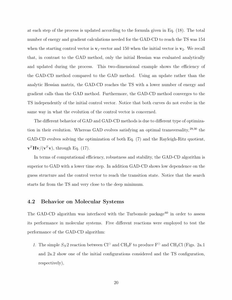
(a) Reactant transition state geometries.

(b) Behavior of location process.

Figure 2: Performance of GAD-CD for the sn2 reaction, Cl+CH3F→ ClCH3+F,(sn2.2.1 and sn2.2.2 runs; see Table 1 for the setup employed in these runs). The dis-tances between F and C and between C and Cl, are shown for the initial structure (a.1)and the converged TS (a.2). The evolution of the energy (in Kcal/mol) and maximum com-ponent in absolute value of the gradient (in Ha/bohr), max{|gµ|}Nµ=1, as a function of thestep number during the TS search for sn2.2.1 (solid lines) and for sn2.2.2(dashed lines) areshown in (b).

24

(a) Reactant transition state geometries.

(b) Behavior of location process.

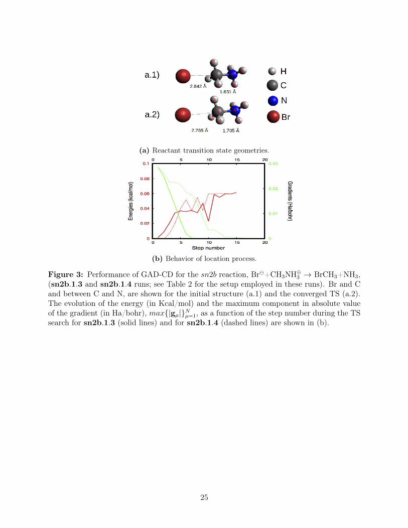
Figure 3: Performance of GAD-CD for the sn2b reaction, Br+CH3NH⊕3 → BrCH3+NH3,(sn2b.1.3 and sn2b.1.4 runs; see Table 2 for the setup employed in these runs). Br and Cand between C and N, are shown for the initial structure (a.1) and the converged TS (a.2).The evolution of the energy (in Kcal/mol) and the maximum component in absolute valueof the gradient (in Ha/bohr), max{|gµ|}Nµ=1, as a function of the step number during the TSsearch for sn2b.1.3 (solid lines) and for sn2b.1.4 (dashed lines) are shown in (b).

25

(a) Reactant transition state geometries.

(b) Behavior of location process.

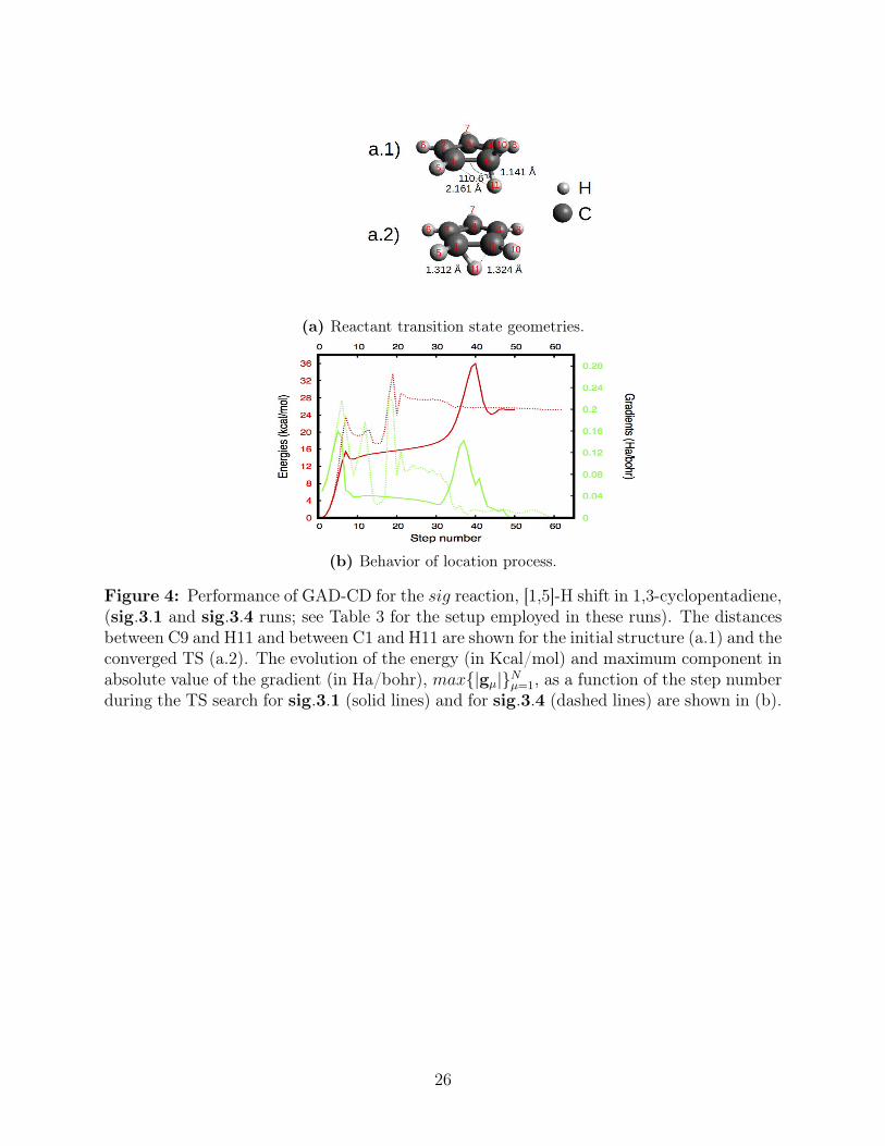
Figure 4: Performance of GAD-CD for the sig reaction, [1,5]-H shift in 1,3-cyclopentadiene,(sig.3.1 and sig.3.4 runs; see Table 3 for the setup employed in these runs). The distancesbetween C9 and H11 and between C1 and H11 are shown for the initial structure (a.1) and theconverged TS (a.2). The evolution of the energy (in Kcal/mol) and maximum component inabsolute value of the gradient (in Ha/bohr), max{|gµ|}Nµ=1, as a function of the step numberduring the TS search for sig.3.1 (solid lines) and for sig.3.4 (dashed lines) are shown in (b).

26

(a) Reactant transition state geometries.

(b) Behavior of location process.

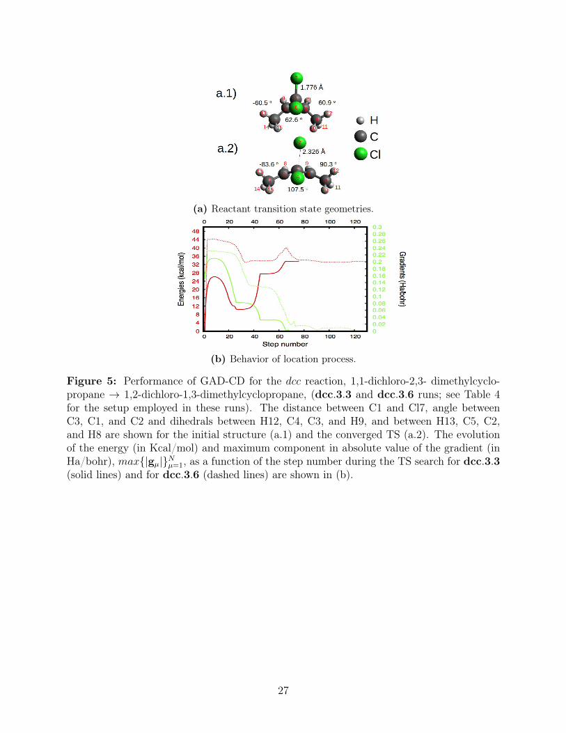
Figure 5: Performance of GAD-CD for the dcc reaction, 1,1-dichloro-2,3- dimethylcyclo-propane → 1,2-dichloro-1,3-dimethylcyclopropane, (dcc.3.3 and dcc.3.6 runs; see Table 4for the setup employed in these runs). The distance between C1 and Cl7, angle betweenC3, C1, and C2 and dihedrals between H12, C4, C3, and H9, and between H13, C5, C2,and H8 are shown for the initial structure (a.1) and the converged TS (a.2). The evolutionof the energy (in Kcal/mol) and maximum component in absolute value of the gradient (inHa/bohr), max{|gµ|}Nµ=1, as a function of the step number during the TS search for dcc.3.3(solid lines) and for dcc.3.6 (dashed lines) are shown in (b).

27

(a) Reactant and transition state geometries.

(b) Behavior of location process.

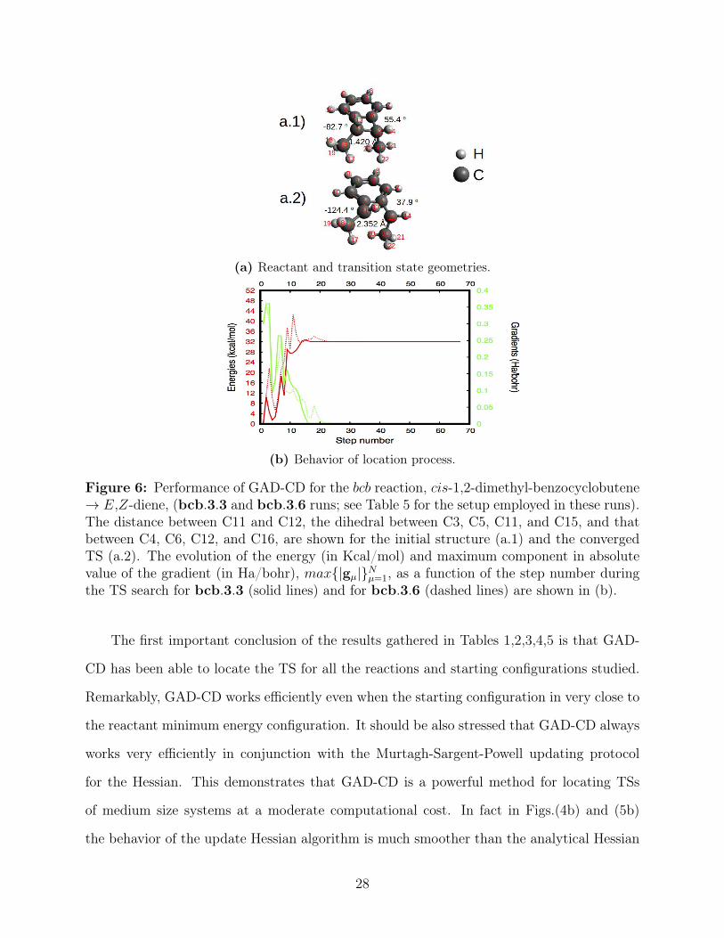
Figure 6: Performance of GAD-CD for the bcb reaction, cis-1,2-dimethyl-benzocyclobutene→ E,Z-diene, (bcb.3.3 and bcb.3.6 runs; see Table 5 for the setup employed in these runs).The distance between C11 and C12, the dihedral between C3, C5, C11, and C15, and thatbetween C4, C6, C12, and C16, are shown for the initial structure (a.1) and the convergedTS (a.2). The evolution of the energy (in Kcal/mol) and maximum component in absolutevalue of the gradient (in Ha/bohr), max{|gµ|}Nµ=1, as a function of the step number duringthe TS search for bcb.3.3 (solid lines) and for bcb.3.6 (dashed lines) are shown in (b).

The first important conclusion of the results gathered in Tables 1,2,3,4,5 is that GAD-

CD has been able to locate the TS for all the reactions and starting configurations studied.

Remarkably, GAD-CD works efficiently even when the starting configuration in very close to

the reactant minimum energy configuration. It should be also stressed that GAD-CD always

works very efficiently in conjunction with the Murtagh-Sargent-Powell updating protocol

for the Hessian. This demonstrates that GAD-CD is a powerful method for locating TSs

of medium size systems at a moderate computational cost. In fact in Figs.(4b) and (5b)

the behavior of the update Hessian algorithm is much smoother than the analytical Hessian

28

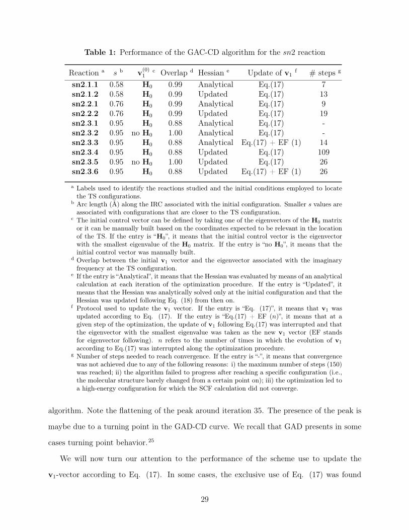
Table 1: Performance of the GAC-CD algorithm for the sn2 reaction

Reaction a s b v(0)1

c Overlap d Hessian e Update of v1f # steps g

sn2.1.1 0.58 H0 0.99 Analytical Eq.(17) 7sn2.1.2 0.58 H0 0.99 Updated Eq.(17) 13sn2.2.1 0.76 H0 0.99 Analytical Eq.(17) 9sn2.2.2 0.76 H0 0.99 Updated Eq.(17) 19sn2.3.1 0.95 H0 0.88 Analytical Eq.(17) -sn2.3.2 0.95 no H0 1.00 Analytical Eq.(17) -sn2.3.3 0.95 H0 0.88 Analytical Eq.(17) + EF (1) 14sn2.3.4 0.95 H0 0.88 Updated Eq.(17) 109sn2.3.5 0.95 no H0 1.00 Updated Eq.(17) 26sn2.3.6 0.95 H0 0.88 Updated Eq.(17) + EF (1) 26

a Labels used to identify the reactions studied and the initial conditions employed to locatethe TS configurations.

b Arc length (Å) along the IRC associated with the initial configuration. Smaller s values areassociated with configurations that are closer to the TS configuration.

c The initial control vector can be defined by taking one of the eigenvectors of the H0 matrixor it can be manually built based on the coordinates expected to be relevant in the locationof the TS. If the entry is “H0”, it means that the initial control vector is the eigenvectorwith the smallest eigenvalue of the H0 matrix. If the entry is “no H0”, it means that theinitial control vector was manually built.

d Overlap between the initial v1 vector and the eigenvector associated with the imaginaryfrequency at the TS configuration.

e If the entry is “Analytical”, it means that the Hessian was evaluated by means of an analyticalcalculation at each iteration of the optimization procedure. If the entry is “Updated”, itmeans that the Hessian was analytically solved only at the initial configuration and that theHessian was updated following Eq. (18) from then on.

f Protocol used to update the v1 vector. If the entry is “Eq. (17)”, it means that v1 wasupdated according to Eq. (17). If the entry is “Eq.(17) + EF (n)”, it means that at agiven step of the optimization, the update of v1 following Eq.(17) was interrupted and thatthe eigenvector with the smallest eigenvalue was taken as the new v1 vector (EF standsfor eigenvector following). n refers to the number of times in which the evolution of v1

according to Eq.(17) was interrupted along the optimization procedure.g Number of steps needed to reach convergence. If the entry is “-”, it means that convergencewas not achieved due to any of the following reasons: i) the maximum number of steps (150)was reached; ii) the algorithm failed to progress after reaching a specific configuration (i.e.,the molecular structure barely changed from a certain point on); iii) the optimization led toa high-energy configuration for which the SCF calculation did not converge.

algorithm. Note the flattening of the peak around iteration 35. The presence of the peak is

maybe due to a turning point in the GAD-CD curve. We recall that GAD presents in some

cases turning point behavior.25

We will now turn our attention to the performance of the scheme use to update the

v1-vector according to Eq. (17). In some cases, the exclusive use of Eq. (17) was found

29

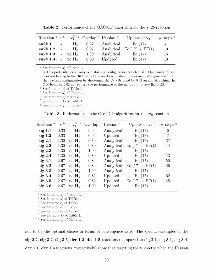
Table 2: Performance of the GAC-CD algorithm for the sn2b reaction

Reaction a s b v(0)1

c Overlap d Hessian e Update of v1f # steps g

sn2b.1.1 - H0 0.97 Analytical Eq.(17) -sn2b.1.2 - H0 0.97 Analytical Eq.(17) + EF(1) 10sn2b.1.3 - no H0 1.00 Analytical Eq.(17) 15sn2b.1.4 - no H0 0.99 Updated Eq.(17) 13

a See footnote a) of Table 1.b In this particular case, only one starting configuration was tested. This configurationdoes not belong to the IRC path of the reaction. Instead, it was manually generated fromthe reactant configuration by shortening the C· · ·Br bond by 0.02 au and stretching theC-N bond by 0.02 au. to test the performance of the method in a very flat PES.

c See footnote c) of Table 1.d See footnote d) of Table 1.e See footnote e) of Table 1.f See footnote f) of Table 1.g See footnote g) of Table 1.

Table 3: Performance of the GAC-CD algorithm for the sig reaction

Reaction a s b v(0)1

c Overlap d Hessian e Update of v1f # steps g

sig.1.1 0.33 H0 0.94 Analytical Eq.(17) 6sig.1.2 0.33 H0 0.94 Updated Eq.(17) 7sig.2.1 1.30 no H0 0.89 Analytical Eq.(17) 37sig.2.2 1.30 no H0 0.89 Analytical Eq.(17) + EF(1) 14sig.2.3 1.30 no H0 1.00 Analytical Eq.(17) -sig.2.4 1.30 no H0 0.89 Updated Eq.(17) 43sig.3.1 2.67 no H0 0.82 Analytical Eq.(17) 50sig.3.2 2.67 no H0 0.82 Analytical Eq.(17) + EF(1) 26sig.3.3 2.67 no H0 1.00 Analytical Eq.(17) -sig.3.4 2.67 no H0 0.82 Updated Eq.(17) 62sig.3.5 2.67 no H0 0.82 Updated Eq.(17) + EF(1) 45sig.3.6 2.67 no H0 1.00 Updated Eq.(17) -

a See footnote a) of Table 1.b See footnote b) of Table 1.c See footnote c) of Table 1.d See footnote d) of Table 1.e See footnote e) of Table 1.f See footnote f) of Table 1.g See footnote g) of Table 1.

not to be the optimal choice in terms of convergence rate. The specific examples of the

sig.2.2, sig.3.2, sig.3.5, dcc.1.2, dcc.1.5 reactions (compared to sig.2.1, sig.3.1, sig.3.4,

dcc.1.1, dcc.1.4 reactions, respectively) show that resetting the v1-vector when the Hessian

30

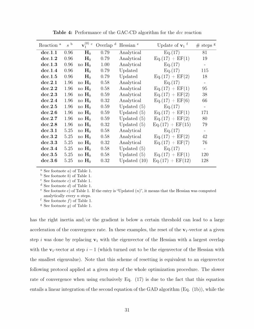
Table 4: Performance of the GAC-CD algorithm for the dcc reaction

Reaction a s b v(0)1

c Overlap d Hessian e Update of v1f # steps g

dcc.1.1 0.96 H0 0.79 Analytical Eq.(17) 81dcc.1.2 0.96 H0 0.79 Analytical Eq.(17) + EF(1) 19dcc.1.3 0.96 no H0 1.00 Analytical Eq.(17) -dcc.1.4 0.96 H0 0.79 Updated Eq.(17) 115dcc.1.5 0.96 H0 0.79 Updated Eq.(17) + EF(2) 18dcc.2.1 1.96 no H0 0.58 Analytical Eq.(17) -dcc.2.2 1.96 no H0 0.58 Analytical Eq.(17) + EF(1) 95dcc.2.3 1.96 no H0 0.59 Analytical Eq.(17) + EF(2) 38dcc.2.4 1.96 no H0 0.32 Analytical Eq.(17) + EF(6) 66dcc.2.5 1.96 no H0 0.59 Updated (5) Eq.(17) -dcc.2.6 1.96 no H0 0.59 Updated (5) Eq.(17) + EF(1) 171dcc.2.7 1.96 no H0 0.59 Updated (5) Eq.(17) + EF(2) 80dcc.2.8 1.96 no H0 0.32 Updated (5) Eq.(17) + EF(15) 79dcc.3.1 5.25 no H0 0.58 Analytical Eq.(17) -dcc.3.2 5.25 no H0 0.58 Analytical Eq.(17) + EF(2) 42dcc.3.3 5.25 no H0 0.32 Analytical Eq.(17) + EF(7) 76dcc.3.4 5.25 no H0 0.58 Updated (5) Eq.(17) -dcc.3.5 5.25 no H0 0.58 Updated (5) Eq.(17) + EF(1) 120dcc.3.6 5.25 no H0 0.32 Updated (10) Eq.(17) + EF(12) 128

a See footnote a) of Table 1.b See footnote b) of Table 1.c See footnote c) of Table 1.d See footnote d) of Table 1.e See footnote e) of Table 1. If the entry is “Updated (n)”, it means that the Hessian was computedanalytically every n steps.

f See footnote f) of Table 1.g See footnote g) of Table 1.

has the right inertia and/or the gradient is below a certain threshold can lead to a large

acceleration of the convergence rate. In these examples, the reset of the v1-vector at a given

step i was done by replacing v1 with the eigenvector of the Hessian with a largest overlap

with the v1-vector at step i− 1 (which turned out to be the eigenvector of the Hessian with

the smallest eigenvalue). Note that this scheme of resetting is equivalent to an eigenvector

following protocol applied at a given step of the whole optimization procedure. The slower

rate of convergence when using exclusively Eq. (17) is due to the fact that this equation

entails a linear integration of the second equation of the GAD algorithm (Eq. (1b)), while the

31

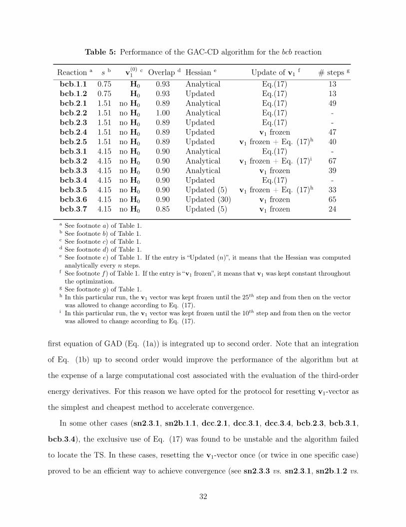
Table 5: Performance of the GAC-CD algorithm for the bcb reaction

Reaction a s b v(0)1

c Overlap d Hessian e Update of v1f # steps g

bcb.1.1 0.75 H0 0.93 Analytical Eq.(17) 13bcb.1.2 0.75 H0 0.93 Updated Eq.(17) 13bcb.2.1 1.51 no H0 0.89 Analytical Eq.(17) 49bcb.2.2 1.51 no H0 1.00 Analytical Eq.(17) -bcb.2.3 1.51 no H0 0.89 Updated Eq.(17) -bcb.2.4 1.51 no H0 0.89 Updated v1 frozen 47bcb.2.5 1.51 no H0 0.89 Updated v1 frozen + Eq. (17)h 40bcb.3.1 4.15 no H0 0.90 Analytical Eq.(17) -bcb.3.2 4.15 no H0 0.90 Analytical v1 frozen + Eq. (17)i 67bcb.3.3 4.15 no H0 0.90 Analytical v1 frozen 39bcb.3.4 4.15 no H0 0.90 Updated Eq.(17) -bcb.3.5 4.15 no H0 0.90 Updated (5) v1 frozen + Eq. (17)h 33bcb.3.6 4.15 no H0 0.90 Updated (30) v1 frozen 65bcb.3.7 4.15 no H0 0.85 Updated (5) v1 frozen 24

a See footnote a) of Table 1.b See footnote b) of Table 1.c See footnote c) of Table 1.d See footnote d) of Table 1.e See footnote e) of Table 1. If the entry is “Updated (n)”, it means that the Hessian was computedanalytically every n steps.

f See footnote f) of Table 1. If the entry is “v1 frozen”, it means that v1 was kept constant throughoutthe optimization.

g See footnote g) of Table 1.h In this particular run, the v1 vector was kept frozen until the 25th step and from then on the vectorwas allowed to change according to Eq. (17).

i In this particular run, the v1 vector was kept frozen until the 10th step and from then on the vectorwas allowed to change according to Eq. (17).

first equation of GAD (Eq. (1a)) is integrated up to second order. Note that an integration

of Eq. (1b) up to second order would improve the performance of the algorithm but at

the expense of a large computational cost associated with the evaluation of the third-order

energy derivatives. For this reason we have opted for the protocol for resetting v1-vector as

the simplest and cheapest method to accelerate convergence.

In some other cases (sn2.3.1, sn2b.1.1, dcc.2.1, dcc.3.1, dcc.3.4, bcb.2.3, bcb.3.1,

bcb.3.4), the exclusive use of Eq. (17) was found to be unstable and the algorithm failed

to locate the TS. In these cases, resetting the v1-vector once (or twice in one specific case)

proved to be an efficient way to achieve convergence (see sn2.3.3 vs. sn2.3.1, sn2b.1.2 vs.

32

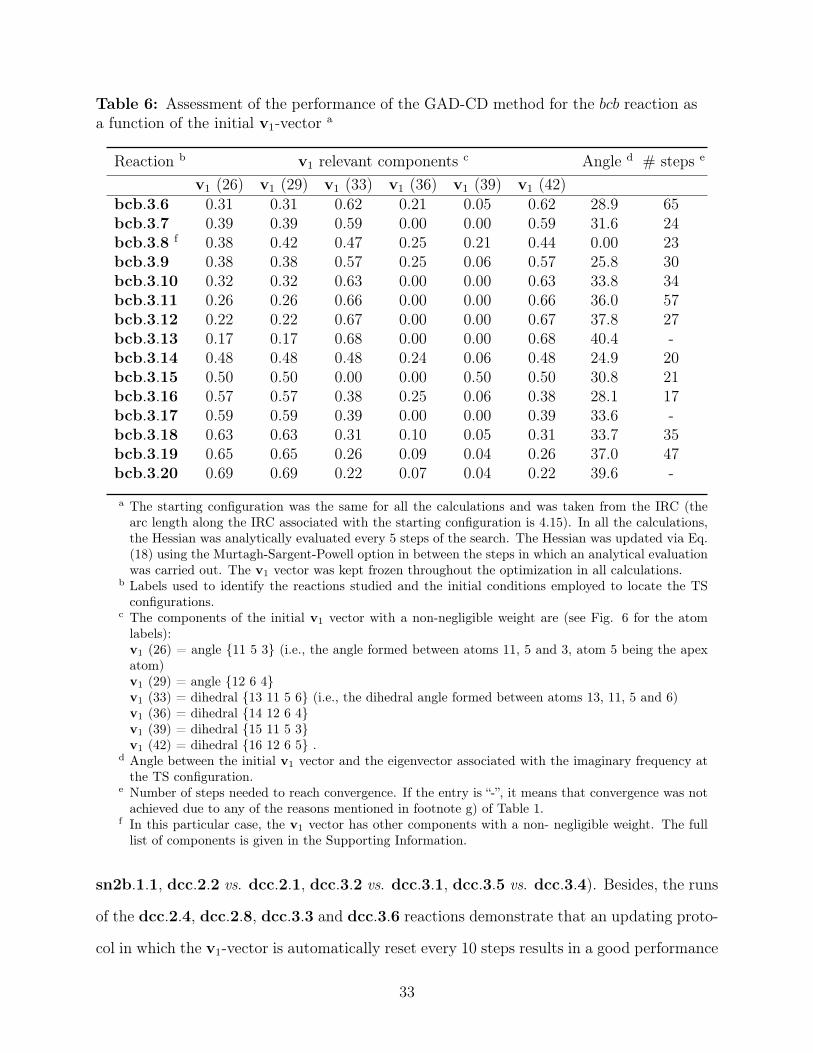
Table 6: Assessment of the performance of the GAD-CD method for the bcb reaction asa function of the initial v1-vector a

Reaction b v1 relevant components c Angle d # steps e

v1 (26) v1 (29) v1 (33) v1 (36) v1 (39) v1 (42)bcb.3.6 0.31 0.31 0.62 0.21 0.05 0.62 28.9 65bcb.3.7 0.39 0.39 0.59 0.00 0.00 0.59 31.6 24bcb.3.8 f 0.38 0.42 0.47 0.25 0.21 0.44 0.00 23bcb.3.9 0.38 0.38 0.57 0.25 0.06 0.57 25.8 30bcb.3.10 0.32 0.32 0.63 0.00 0.00 0.63 33.8 34bcb.3.11 0.26 0.26 0.66 0.00 0.00 0.66 36.0 57bcb.3.12 0.22 0.22 0.67 0.00 0.00 0.67 37.8 27bcb.3.13 0.17 0.17 0.68 0.00 0.00 0.68 40.4 -bcb.3.14 0.48 0.48 0.48 0.24 0.06 0.48 24.9 20bcb.3.15 0.50 0.50 0.00 0.00 0.50 0.50 30.8 21bcb.3.16 0.57 0.57 0.38 0.25 0.06 0.38 28.1 17bcb.3.17 0.59 0.59 0.39 0.00 0.00 0.39 33.6 -bcb.3.18 0.63 0.63 0.31 0.10 0.05 0.31 33.7 35bcb.3.19 0.65 0.65 0.26 0.09 0.04 0.26 37.0 47bcb.3.20 0.69 0.69 0.22 0.07 0.04 0.22 39.6 -

a The starting configuration was the same for all the calculations and was taken from the IRC (thearc length along the IRC associated with the starting configuration is 4.15). In all the calculations,the Hessian was analytically evaluated every 5 steps of the search. The Hessian was updated via Eq.(18) using the Murtagh-Sargent-Powell option in between the steps in which an analytical evaluationwas carried out. The v1 vector was kept frozen throughout the optimization in all calculations.

b Labels used to identify the reactions studied and the initial conditions employed to locate the TSconfigurations.

c The components of the initial v1 vector with a non-negligible weight are (see Fig. 6 for the atomlabels):v1 (26) = angle {11 5 3} (i.e., the angle formed between atoms 11, 5 and 3, atom 5 being the apexatom)v1 (29) = angle {12 6 4}v1 (33) = dihedral {13 11 5 6} (i.e., the dihedral angle formed between atoms 13, 11, 5 and 6)v1 (36) = dihedral {14 12 6 4}v1 (39) = dihedral {15 11 5 3}v1 (42) = dihedral {16 12 6 5} .

d Angle between the initial v1 vector and the eigenvector associated with the imaginary frequency atthe TS configuration.

e Number of steps needed to reach convergence. If the entry is “-”, it means that convergence was notachieved due to any of the reasons mentioned in footnote g) of Table 1.

f In this particular case, the v1 vector has other components with a non- negligible weight. The fulllist of components is given in the Supporting Information.

sn2b.1.1, dcc.2.2 vs. dcc.2.1, dcc.3.2 vs. dcc.3.1, dcc.3.5 vs. dcc.3.4). Besides, the runs

of the dcc.2.4, dcc.2.8, dcc.3.3 and dcc.3.6 reactions demonstrate that an updating proto-

col in which the v1-vector is automatically reset every 10 steps results in a good performance

33

in terms of convergence rate.

In a few cases of the bcb reaction (bcb2.3, bcb.3.1 and bcb3.4 reactions), the v1-vector

featured an unexpected evolution. Specifically, it was observed that this vector becomes very

different with respect to the desired eigenvector of the Hessian matrix as the TS search goes

on. This resulted in a “corrupted” control vector with large weights on components that

are not chemically relevant to drive the reaction, thus leading to failure to locate the TS.

Freezing the v1-vector during the initial steps of the search proved to be an efficient way to

overcome this problem and achieve convergence (see bcb2.5, bcb3.2, bcb3.5) and in some

cases the algorithm converges even if the v1-vector is kept frozen during the whole process

(see bcb2.4, bcb3.3, bcb3.6 and bcb3.7).

Another important aspect of the GAD-CD algorithm is its performance as a function

of the initial choice for the v1-vector. In order to assess such performance, we took the

third starting configuration (i.e, the one lying closer to the reactants configuration) of the

bcb system and we carried out multiple GAD-CD runs with different initial definitions of

the v1-vector for the same starting configuration. As shown in Table 6, there is a wide

range of initial v1 vectors that lead to the same TS. This demonstrates that GAD-CD is a

robust and versatile method for locating TS in molecular systems (see section 5 of Supporting

Information for further evidence).

Finally, we focus on the strong and weak points of the new proposed method compared to

other methods existing in the literature. As explained in Section 2, the family of techniques

based on an eigenvector-following philosophy is one of the most widely used families to locate

TSs. One of the algorithms that fall within this set is the TRIM algorithm70 (implemented,

for instance, in Turbomole60 code). From a conceptual point of view, TRIM is, within the

family of eigenvector following techniques, the closest one to GAC-CD. The main difference

between these two techniques is the way in which the guiding vector is updated during

the location process. A numerical comparison between GAD-CD and the standard TRIM

methods is reported in Section 6 of the Supporting Information. When considering initial

34

configurations close to the TS, the performance of GAD-CD is quite similar to that of

TRIM. In some of the tested cases, GAD-CD takes a few extra iterations (less than 10) to

converge compared to TRIM. This is not surprising if one takes into account that TRIM

was specifically designed for situations in which the initial configuration is close to the TS.

However, the main advantage of GAD-CD over TRIM emerges when considering initial

configurations that are very close to reactants. Indeed, GAD-CD is able to locate the TS of

all systems considered in this study when starting close to reactants (see Tables 1,2,3, and

4), while TRIM fails to do so in the most complex systems (dcc and bcb) even when the full

Hessian is evaluated at each point.

Let us stress again that GAD-CD behaves well even when the Hessian is updated and not

analytically computed, thus making the technique very efficient. The limitations of TRIM

when starting far away from the TS stem from the fact that this method was not designed

to locate TSs in such cases. In fact, it is usually recommended (see, e.g., the manual of

Turbomole60) to use a “double-ended” method to generate an initial guess structure prior to

using TRIM to ensure convergence to the desired TS. In contrast, GAD-CD does not need

the preliminary calculation and works well even when starting from just one of the minima

of the PES. Overall, we conclude that the GAD-CD algorithm possesses good numerical

stability and computational efficiency. Finally, the control over the initial v1-vector together

with the low computational cost associated with the updated Hessian protocol renders GAD-

CD a very powerful method for the automatic exploration of complex PESs by parallel runs

with different initial v1 vectors from a given basin of the PES.

5 Conclusions

We have reported an algorithm, called GAD-CD, to locate saddle points of index one on

multidimensional PESs. This method can be considered an extension of the GAD method

to quadratic order using a restricted step technique and a set of conjugate directions with

35

respect to the Hessian matrix. It is shown that the GAD-CD method is more robust than

the GAD method, requiring not only a smaller number of energy and gradient calculations,

but also achieving converged results independently of the initial control vector in situations

where the GAD method fails to capture the corresponding TS. Although the present form of

the GAD-CD has a higher computational cost than GAD (due to an extra diagonalization at

each step), there may be different ways to make GAD-CD more efficient. This is currently

being investigated.

The GAD-CD method is easily interfaced with standard quantum-chemistry software

such as the widely-spread Turbomole package,60 and provides converged results within a

relatively small number of iteration steps. This has been proven by means of five medium

size molecular systems for which GAD-CD works efficiently even when starting close to

the reactant minima. Its performance remains optimal even when fast updating Hessian

protocols are employed. This opens the door to an automatic exploration of complex PESs.

Hence, we envision our GAD-CD method as being implemented in standard quantum-

chemistry packages and become a useful tool for the localization of transition states in

multidimensional PESs, especially in situations where the high complexity of the associated

topographies difficult the definition of an educated guess structure, close enough to the TS

to be located by standard algorithms.

Acknowledgement

The authors thank to the financial support from the Spanish Ministerio de Economía y

Competitividad, Projects No. CTQ2016-76423-P, CTQ2017-87773-P and Spanish Structures

of Excellence María de Maeztu program through grant MDM-2017-0767 and Generalitat de

Catalunya, Project No. 2017 SGR 348. G.A. acknowledges also financial support from

the European Union’s Horizon 2020 research and innovation programme under the Marie

Sklodowska-Curie grant agreement No 752822.

36

Supporting Information Available

The following files are available free of charge.

• The supporting information file includes:

1. Sets of internal coordinates employed in the calculations of molecular systems.

2. Initial configurations given in both cartesian and internal coordinates.

3. Transition state configurations given in both cartesian and internal coordinates.

4. Initial v1 vectors for all runs.

5. Extra assessments of the performance of GAD-CD as a function of the initial

v1-vector.

6. Comparison between the GAD-CD and TRIM algorithms.

• The code including the interface between GAD-CD and Turbomole60 can be provided

free of charge upon request to one of the corresponding authors.

This material is available free of charge via the Internet at http://pubs.acs.org/.

References

(1) E, W.; Zhou, X. Nonlinearity 2011, 24, 1831–1842.

(2) Liu, B. J. Chem. Phys. 1973, 58, 1925 – 1937.

(3) O’Neil, S. V.; Pearson, P. K.; Schaefer III, H. F.; Bender, C. F. J. Chem. Phys. 1973,

58, 1126 – 1132.

(4) Rothman, M. J.; Lohr, L. L. Chem. Phys. Lett. 1980, 70, 405 – 409.

(5) Williams, I. H.; Maggiora, G. M. J. Mol. Struct. (Theochem) 1982, 89, 365–378.

(6) Quapp, W.; Hirsch, M.; Imig, O.; Heidrich, D. J. Comput. Chem. 1998, 19, 1087–1100.

37

(7) Anglada, J. M.; Besalú, E.; Bofill, J. M.; Crehuet, R. J. Comput. Chem. 2001, 22,

387–406.

(8) Crehuet, R.; Bofill, J. M.; Anglada, J. M. Theor. Chem. Acc. 2002, 107, 130–139.

(9) Hirsch, M.; Quapp, W. J. Math. Chem. 2004, 36, 307–340.

(10) Bofill, J. M.; Quapp, W. J. Chem. Phys. 2011, 134, 074101.

(11) Basilevsky, M.; Shamov, A. Chemical Physics 1981, 60, 347–358.

(12) Hoffmann, D. K.; Nord, R. S.; Ruedenberg, K. Theor. Chim. Acta 1986, 69, 265–280.

(13) Quapp, W. Theor. Chim. Acta 1989, 75, 447 – 460.

(14) Sun, J.-Q.; Ruedenberg, K. J. Chem. Phys. 1993, 98, 9707–9714.

(15) Bofill, J. M.; Quapp, W.; Caballero, M. J. Chem. Theory Comput. 2012, 8, 927–935.

(16) McIver, Jr., J. W.; Komornicki, A. J. Am. Chem. Soc. 1972, 94, 2625 – 2633.

(17) Poppinger, D. Chem. Phys. Lett. 1975, 35, 550 – 554.

(18) Bofill, J. M.; Ribas-Ariño, J.; García, S. P.; Quapp, W. J. Chem. Phys. 2017, 147,

152710 – 152719.

(19) Crippen, G. M.; Scheraga, H. A. Arch. Biochem. Biophys. 1971, 144, 462 – 466.

(20) Pedersen, A.; Hafstein, S. F.; Jónsson, H. SIAM J. Sci. Comput. 2011, 33, 633 – 652.

(21) Cerjan, C. J.; Miller, W. H. J. Chem. Phys. 1981, 75, 2800 – 2806.

(22) Henkelman, G.; Jónsson, H. J. Chem. Phys. 1999, 111, 7010 – 7022.

(23) Ohno, K.; Maeda, S. Chem. Phys. Lett. 2004, 384, 277 – 282.

(24) Shang, C.; Liu, Z.-P. J. Chem. Theory Comput. 2012, 8, 2215 – 2222.

38

(25) Bofill, J. M.; Quapp, W.; Caballero, M. Chem. Phys. Lett. 2013, 583, 203–208.

(26) Samanta, A.; E, W. J. Chem. Phys. 2012, 136, 124104 – 124114.

(27) Quapp, W.; Bofill, J. M. Theor. Chem. Acc. 2014, 133, 1510 – 1523.

(28) Bofill, J. M.; Quapp, W.; Bernuz, E. J. Math. Chem. 2015, 53, 41 – 57.

(29) Bofill, J. M.; Quapp, W. Theor. Chem. Acc. 2016, 135, 11 – 24.

(30) Albareda, G.; Bofill, J. M.; de P.R. Moreira, I.; Quapp, W.; Rubio-Martínez, J. Theor.

Chem. Acc. 2018, 137, 73 – 82.

(31) Fletcher, R. Practical Methods of Optimization; Wiley-Interscience, New York, 1987.

(32) Schlegel, H. B. J. Comput. Chem. 1982, 3, 214 – 218.

(33) Hratchian, H. P.; Schlegel, H. B. In Theory and Applications of Computational Chem-

istry ; Dykstra, C. E., Frenking, G., Kim, K. S., Scuseria, G. E., Eds.; Elsevier: Ams-

terdam, 2005; pp 195–249.

(34) Simons, J.; Jørgensen, P.; Taylor, H.; Ozment, J. J. Phys. Chem. 1983, 87, 2745 –

2753.

(35) Banerjee, A.; Adams, N.; Simons, J.; Shepard, R. J. Phys. Chem. 1985, 89, 52 – 57.

(36) Baker, J. J. Comput. Chem. 1986, 7, 385 – 395.

(37) Culot, P.; Dive, G.; Nguyen, V. H.; Ghuysen, J. M. Theor. Chim. Acta 1992, 82, 189

– 205.

(38) Anglada, J. M.; Bofill, J. M. Int. J. Quantum Chem. 1997, 62, 153 – 165.

(39) Besalú, E.; Bofill, J. M. Theor. Chem. Acc. 1998, 100, 265 – 274.

(40) Sinclair, J. E.; Fletcher, R. J. Phys. C: Solid State Phys. 1974, 7, 864 – 870.

39

(41) Bell, S.; Crighton, J. S.; Fletcher, R. Chem. Phys. Lett. 1981, 82, 122 – 126.

(42) Bell, S.; Crighton, J. S. J. Chem. Phys. 1984, 80, 2464 – 2475.

(43) Halgren, T. A.; Lipscomb, W. N. Chem. Phys. Lett. 1977, 49, 225 – 232.

(44) Peng, C.; Schlegel, H. Isr. J. Chem. 1993, 33, 449 – 454.

(45) Peters, B.; Heyden, A.; Bell, A. T.; Chakraborty, A. J. Chem. Phys. 2004, 120, 7877

– 7886.

(46) Quapp, W. J. Comput. Chem 2007, 28, 1834–1847.

(47) Crehuet, R.; Bofill, J. M. J. Chem. Phys. 2005, 122, 234105–234120.

(48) Aguilar-Mogas, A.; Crehuet, R.; Giménez, X.; Bofill, J. M. Mol. Phys. 2007, 105, 19 –

22.

(49) Quapp, W. J. Theor. Comput. Chem. 2009, 8, 101 – 117.

(50) Aguilar-Mogas, A.; Giménez, X.; Bofill, J. M. J. Comput. Chem. 2010, 31, 2510 – 2525.

(51) Avdoshenko, S. M.; Makarov, D. E. J. Phys. Chem. B 2016, 120, 1537 – 1545.

(52) Zimmerman, P. M. J. Comput. Chem. 2015, 36, 601 – 611.

(53) Powell, M. J. D. Comput. J. 1964, 7, 155 – 162.

(54) Greenstadt, J. Math. Comp. 1970, 24, 1 – 22.

(55) Powell, M. J. D. J. Inst. Maths. Applns. 1971, 7, 21 – 36.

(56) Bofill, J. M. J. Comput. Chem. 1994, 15, 1–11.

(57) Bofill, J. M.; Comajuan, M. J. Comput. Chem. 1995, 16, 1326 – 1338.

(58) Anglada, J. M.; Bofill, J. M. J. Comput. Chem. 1998, 19, 349 – 362.

40

(59) Bofill, J. M. Int. J. Quantum Chem. 2003, 94, 324 – 332.

(60) Ahlrichs, R.; Bär, M.; Häser, M.; Horn, H.; Kölmel, C. Chem. Phys. Lett. 1989, 162,

165 – 169.

(61) Müller, K.; Brown, L. Theor. Chem. Acc. 1979, 53, 75 – 93.

(62) Press, W. H.; Teukolsky, S. A.; Vetterling, W. T.; Flannery, B. P. Numerical Recipes

in Fortran 77: The Art of Scientific Computing ; Cambridge University Press, 1992.

(63) Roth, W. R. Tetrahedron Lett. 1964, 1009 – 1013.

(64) Woodward, R. B.; Hoffmann, R. Angew. Chem. Int. Ed. Engl. 1969, 8, 781 – 853.

(65) Selms, R. C. D.; Combs, C. M. J. Org. Chem. 1963, 28, 2206 – 2210.

(66) Huisgen, R.; Seidel, H. Tetrahedron Lett. 1964, 3381 – 3386.

(67) Quinkert, G.; Opitz, K.; Wiersdorff, W. W.; Finke, M. Tetrahedron Lett. 1965, 3009 –

3016.

(68) Becke, A. J. Chem. Phys. 1993, 98, 5648 – 5652.

(69) Schäfer, A.; Horn, H.; Ahlrichs, R. J. Chem. Phys. 1993, 97, 2571 – 2577.

(70) Helgaker, T. Chem. Phys. Lett. 1991, 182, 503 – 510.

41

Graphical TOC Entry

Gentlest Ascent Dynamics and Conjugate Direction: GAD-CD.The set of arrows shows the evolution of the control vectorfrom an arbitrary guess point to the Transition State in the

Potential Energy Surface.

42