is china’s p/e ratio too low? examining the role of...
TRANSCRIPT

Is China’s P/E Ratio too Low? Examining the Role of Earnings Volatility
Alan G. Huang† and Tony S. Wirjanto‡
This Version: July, 2011
Abstract
We find that China’s P/E ratio is comparable to that of the U.S. S&P 1500 index,
a broad based index covering large, middle, and small capitalization firms. We provide an
explanation as to why China’s seemingly low P/E ratio is not surprising in light of the
economic growth that it has experienced. Specifically, we show that (i) the P/E ratio is
negatively associated with earnings volatility in both the Chinese and U.S. stock markets
with an economically significant magnitude; and (ii) historical earnings volatility is
considerably higher in China than in the U.S. Higher earnings volatility in China offsets
higher growth prospect in setting the P/E ratio, making its P/E ratio much closer to what
is observed empirically than otherwise implied by its growth rate.
JEL Classification: G15, G13, G32 Keywords: P/E ratio; China; U.S.; earnings volatility
† (Corresponding author) School of Accounting and Finance, University of Waterloo, Waterloo, ON N2L 3G1 Canada, email: [email protected], tel: 519-888-4567 ext. 36770, and fax: 519-888-7562. ‡ School of Accounting and Finance, and Department of Statistics and Actuarial Science, University of Waterloo, Waterloo, ON N2L 3G1 Canada, email: [email protected], tel: 519-888-4567 ext. 35210.

Is China’s P/E Ratio too Low?
Examining the Role of Earnings Volatility
Abstract
We find that China’s P/E ratio is comparable to that of the U.S. S&P 1500 index, a broad
based index covering large, middle, and small capitalization firms. We provide an explanation as
to why China’s seemingly low P/E ratio is not surprising in light of the economic growth that it
has experienced. Specifically, we show that (i) the P/E ratio is negatively associated with earnings
volatility in both the Chinese and U.S. stock markets with an economically significant magnitude;
and (ii) historical earnings volatility is considerably higher in China than in the U.S. Higher
earnings volatility in China offsets higher growth prospect in setting the P/E ratio, making its P/E
ratio much closer to what is observed empirically than otherwise implied by its growth rate.

1
1. Introduction
Measuring the price per unit of net income, the price to earnings (P/E) ratio is arguably
one of the most widely used valuation metrics in the financial markets. In traditional textbook
models of corporate finance, such as the Gordon growth model, a higher growth rate implies a
larger P/E ratio since growth rate is positively related to price. Because growth rates in emerging
markets are generally higher than in mature markets, stocks in emerging market are expected to
command higher P/E ratios. It follows that when the Chinese stock markets experienced a
dramatic drop recently, with the Shanghai Composite index falling from the peak of 6,092 on
October 16, 2007 to the bottom of 1,719 on November 3, 2008, many observers of financial
markets have come to argue that the Chinese markets are undervalued on the basis that China has
a P/E ratio comparable to or lower than that in prevailing mature markets, in particular, the U.S.
markets.1
Interestingly, we find that a comparable level of P/E ratio between China and the U.S. is
not unique to the above declining period in China. Instead, a comparison of the historical P/E
ratio between the U.S. and China reveals no substantive difference between the two markets. For
instance, in the period from 1997 to 2007, the U.S. S&P 1500 index firms had a market-wide P/E
ratio of 20.81. In the same period, China had a market-wide P/E ratio of 25.03. A null hypothesis
that China’s P/E ratio is 20% higher than that of the U.S. cannot be rejected at the 5%
significance level. Similar results are obtained when we use firm-level P/E ratios. This small
difference does not seem to reflect the phenomenal economic growth that China has experienced
1 Much of this argument has appeared in popular press. For example, Financial Times reported on June 27,
2008 that: “Yang Yu, the manager of the Harvest Shanghai-Shenzhen 300 Index Fund, yesterday showed
his confidence in the prospect of the A-share market, chiefly because the weighted average price-earnings
ratio (P/E ratio) of the Shanghai-Shenzhen 300 Index had reached about 16 times by June 20, 2008, close to
the international level.”

2
during the past three decades if we base our calculations on traditional pricing formulae.2 It is,
therefore, puzzling to observe that China’s P/E ratio is not much higher than that of the U.S.
This paper provides a simple but intuitive explanation as to why an emerging market such
as China may not require a much higher P/E valuation than a mature market such as the U.S. Our
proposed explanation is based on the volatility of fundamental earnings. In general, volatile
earnings entail higher risk and thus a higher cost of equity, therefore depressing valuation ratios
in a standard discounted cash flow framework. Recent literature provides evidence for the
negative association between operating volatility and valuation ratios. Rountree, Weston, and
Allayannis (2008) show that cash flow volatility is negatively related to Tobin’s q; and the
literature on income smoothing also documents that various forms of income smoothing lead to
higher valuation metrics, of particular interest among which, earnings volatility has a negative
impact on market value (Allayannis and Simko, 2009) and price to earnings ratio (Hunt, Moyer,
and Shelvin, 2005). Last but not the least, in a study closely related to ours, Thomas and Zhang
(2007) directly confirm that a negative relation between P/E and earnings volatility exists for a
large sample of U.S. firms.
We first extend Thomas and Zhang (2007) and show that the P/E ratio is strongly and
inversely related to earnings volatility not only in the U.S. but also in China. While Chinese firms
are expected to have higher growth rates (as implied by its GDP growth), earnings volatility in
China is much higher than in the U.S. These two quantities have a countervailing effect on the
P/E ratio. Specifically, while an expected higher growth rate implies a higher P/E ratio, higher 2 In the presence of growth, the P/E ratio can be written as: ),/()1(/ gkgEP where k is the cost of
equity capital, and g is the growth rate. The U.S. experience is that k is about 7% and g is about 2%, so that
the market-wide P/E is about 20. China’s GDP growth rate has been in the range of 7-9% in the past three
decades. Professor Asmath Damodaran of New York University estimates that China’s long-term country
risk premium is 1.2% and short-term country risk premium is 4%. Using the mean of these two country risk
premium estimates—2.6%, and a low end of growth rate of 7%, the P/E ratio of China should be 41.

3
earnings volatility leads to a lower P/E ratio. Given the well-known pitfalls in comparing P/E
ratios across countries and across time, we also provide evidence that the documented
relationship is robust to a number of proxies for earnings volatility and the P/E ratio, and survives
the controls of firm growth prospects and Fama-French three factors of market, book to market
and size.
The impact of earnings volatility on the P/E ratio is economically significant. In
particular, China not only has larger earnings volatility than the U.S., its P/E ratio is also more
sensitive to earnings volatility. As a result, a much larger portion of the P/E ratio is negatively
affected by earnings volatility in China than in the U.S. We estimate that relative to the U.S.,
earnings volatility additionally reduces China’s P/E ratio by the order of six, making China’s P/E
ratio much closer to that of the U.S., and to what is observed empirically than otherwise implied
by its growth rate.
This paper contributes to the literature in two major ways. Firstly, we point out that the
overall P/E ratio of the Chinese markets is actually close to, rather than much higher than (as is
usually perceived in popular press), the P/E ratio of the U.S. markets. It is interesting to note that
China’s P/E ratio is frequently discussed in popular press but rarely studied in the academic
setting. We attempt to fill this gap by using a comprehensive dataset covering the Chinese
markets. Secondly, we propose to explain the closeness of P/E ratio between the U.S. and China
by earnings volatility. In related studies, Kane, Marcus and Noh (1996) show that the market-
wide U.S. P/E ratio is negatively associated with the market return volatility, and Thomas and
Zhang (2007) document a negative relation between earnings volatility and P/E. We extend these
studies and show that variations in the sensitivity of the P/E ratio to earnings volatility across U.S.
and China are able to explain the seemingly small gap of P/E ratio between the two countries. To

4
the best of our knowledge, this is the first study of its kind.3 Our results can also be extended to
other emerging markets, where earnings volatility is similarly high and P/E ratio may be
negatively affected in a similar fashion.
The remainder of the paper is organized as follows. Section 2 compares the market-wide
and firm-level P/E ratios of the U.S. and Chinese markets. This is followed by a set of regression
analysis to show the sensitivity of the P/E ratio to earnings volatility in Section 3. Section 4
conducts a number of robustness checks, including an alternative valuation metric of the
price/earnings to growth (PEG) ratio, alternative measures of earning volatility and P/E ratio, and
additional considerations on outlier effects and potential scalar problem. Lastly, Section 5
provides some concluding remarks.
2. Market-Wide and Firm-Specific P/E Ratio Differences between China and the U.S.
2.1 Samples
Our China sample is retrieved from the CSMAR (China Stock Market & Accounting
Research) Database, where the coverage of firm accounting and trading data begins in 1991, the
inception year of the stock markets in China. Although the data provides coverage from 1991,
prior to 1995 the markets (both Shenzhen and Shanghai stock exchanges) had only a few listed
firms. Consequently we choose our Chinese sample to start from 1995. Allowing for two years
for the estimation of earnings volatility (to be elaborated later), our Chinese data starts from 1997.
Domestically listed Chinese firms float either A-shares, which are denominated in local
currency (Chinese Yuan), or B-shares, which are denominated in Hong Kong dollar (Shenzhen
3 We searched the ProQuest database with the following two key phrases: “P/E ratio”, and “China”. We
were not able to find academic papers that focus on the Chinese P/E ratio. We also searched these two
phrases in both Google standard and Google Scholar and failed to find such academic papers in the first ten
pages of the search results.

5
Stock Exchange) or U.S. dollar (Shanghai Stock Exchange), or both. The B-share market
accounts for only a small part of the Chinese stock markets, is very illiquid, and has a low P/E
ratio.4 For this reason, we focus on the A-share markets in this paper and exclude firms whose
share structure includes B-shares.
Table I provides the number of firms in our China sample by year after the above screens.
We note that some of the firms drop out due to missing accounting data items. As a result, the
number of the sample firms is slightly smaller than the actual number of listed firms. For example,
at the end of 2007, there were 1,439 firms that listed A-shares. 1,397 of them are included in our
sample.
[Table I about here.]
For the U.S. market, we select the S&P Composite 1500 firms. S&P 1500 covers
approximately 85% of the U.S. market capitalization and combines S&P 500, S&P 400, and S&P
600, which correspond, respectively, to large cap, mid cap and small cap stocks. We choose the
same time period of 1997-2007 for the U.S. sample. The accounting data and stock prices of the
S&P 1500 firms are obtained from Standard and Poor’s Compustat and CRSP, respectively.
Choosing the full sample of China and S&P 1500 for the U.S. provides a suitable match
between the two countries, as both samples cover all sizes of firms. We highlight this point
because a comparison of P/E ratio between China and the U.S. is frequently drawn on the full
sample of the Chinese markets versus S&P 500. As S&P 500 consists of only large firms, such a
comparison may induce a bias if the P/E ratio is related to firm size, as is commonly believed.
4 As of the end of 2007, in the CSMAR data base, there are 106 B-shares firms with a tradable-share
market value of 247 billion Chinese Yuan (with the end-of-year exchange rate of 0.93 Yuan per HK$ and
7.30 Yuan per US$), and 1,439 A-share firms with a tradable-share market value of 9 trillion Yuan. For a
description of the B-share markets, see, e.g., Chan, Menkveld, and Yang (2008).
6
2.2 A Comparison of Market-Wide P/E between China and the U.S.
Figure 1 plots the monthly market-wide P/E ratio for the U.S. and China over our sample
period. In the figure, the market-wide P/E ratio for month t is calculated as:
,
,
,
N
iti
N
iti
Earnings
ME (1)
where N is the number of firms at time t, ME is the market equity of firm i at month t,5 and
Earnings is the trailing 12-month operating earnings.6 The use of operating earnings is consistent
with the literature (see e.g., Thomas and Zhang, 2007); and throughout the paper, we refer to
earnings as earnings from operations. Since at the firm level, negative P/E is not a meaningful
valuation metric (see, e.g., Easton, 2004), we drop all of the observations with negative earnings
from the calculation of market-wide P/E ratio.
[Figure 1 about here.]
We make several observations from Figure 1. First, the P/E ratios of China and the U.S.
tend to move together. As a matter of fact, the (unconditional) correlation of the P/E ratio
between China and the U.S. is as high as 0.74. Second, on average the P/E ratio of China is not
much higher than that of U.S. China’s P/E ratio is higher than that of the U.S. prior to 2003 but is
5 There are two types of shares in China for our sample period: tradable shares that are publicly traded and
non-tradable shares that are privately traded. The market equity of a Chinese firm is calculated as the
product of its market price and its number of total shares outstanding. This calculation assumes that there
is no pricing difference between tradable and non-tradable shares. In reality, this needs not be the case, see,
e.g., Huang and Fung (2005). Using tradable shares only and the pro-rata earnings does not change our
conclusions.
6 To calculate the trailing 12-month earnings, we use quarterly earnings for the U.S. sample and interim
(half-year frequency) earnings for the China sample. We use the interim data for the China sample because
quarterly accounting data were not reported prior to 2002.

7
typically lower than that of the U.S. post 2003. The lower P/E ratio of China post 2003, of course,
reflects the fact that China experienced an extended bear market during that period.
A notable exception in Figure 1 is that China experiences an abnormally high market-
wide P/E in the first half of 1998. This is due to the Asian Financial Crisis, which caused a wide
spread of losses among Chinese firms. For that period, only 101 firms out of the 594 sample firms
survive the screen of positive earnings; furthermore, these positive earnings tend to be small in
magnitude. In contrast, in the second half of 1998, 605 out of the 689 sample firms survive the
positive-earnings screen.
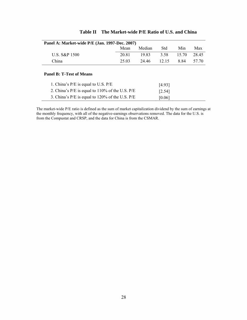
Table II further illustrates the similarity of the P/E ratio between the two markets. Over
the sample period, the mean P/E ratio of the U.S. is 20.81, and of China is 25.03 (Panel A),
indicating that the average value of the market-wide P/E ratio in China is not too much higher
than its counterpart in the U.S.
[Table II about here.]
In Panel B of Table II, we conduct several t-tests for the difference in the mean P/E
between the two countries. Unconditionally, China’s P/E ratio is greater than the U.S. P/E ratio (t-
statistic = 4.93). While the null hypothesis that China’s P/E ratio is equal to 110% of the U.S. P/E
is rejected (t-statistic = 2.54), the null that China’s P/E ratio is 120% of the U.S. P/E is not
rejected (t-statistic of only 0.06).7 In sum, Figure 1 and Table II lead us to conclude that China’s
market-wide P/E ratio is only slightly higher than that of the U.S.
2.3 A Comparison of Firm-Level P/E between China and the U.S.
We now compare the firm-level P/E ratio between China and the U.S. The main
explanatory variable in this paper, earnings volatility, is calculated as the standard deviation of
earnings over the past three years. To match the estimation window of earnings volatility, we use
7 We note that similar test results apply to the median value of the P/E ratio.

8
the average earnings over the same period to calculate individual P/E ratios. Thus, we define
firm-level P/E ratio as a firm’s market equity at the end of the accounting period divided by the
average 12-month trailing earnings over the past three years. We note that although the use of the
average three-year earnings is somewhat unorthodox, in the robustness checks section we report
that our findings are robust to the use of the traditional trailing 12-month earnings measure. As
previously noted, all negative P/E observations have been removed from the sample.
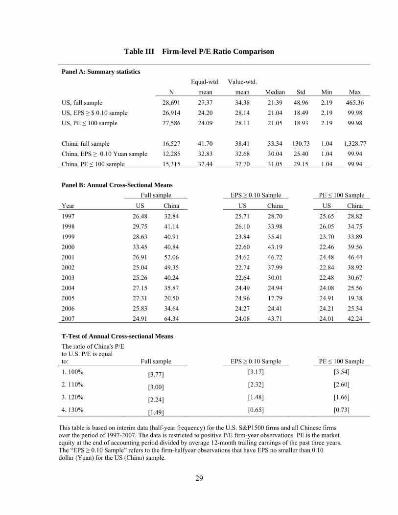
Table III shows the firm-level P/E comparison between the U.S. and China. We first
report the full sample comparison in Panel A and make several observations there. First, the
unconditional mean of firm-specific P/E is larger than the market-wide P/E documented in Table
II for both countries. This is due to small earnings in the individual P/E ratio calculation. The
small earnings problem is particularly acute in China, as firms frequently manage earnings to
report small positive earnings, a fact well documented in the literature.8 This leads to an
extremely high standard deviation in China’s P/E (130.73), and inadvertently makes the equal-
weighted mean of China’s P/E appear much larger than that of the U.S. over the full sample
(41.70 for China vs. 27.37 for the U.S.).
[Table III about here.]
To ameliorate the small earnings problem, we further examine, respectively, the P/E ratio
in two subsamples consisting of the observations with: (1) EPS no smaller than 0.10 USD (Yuan)
for the U.S. (China), and (2) P/E ratio less than 100. As shown in Panel A of Table III, restricting
EPS to no smaller than 0.10 results in a loss of 6% (26%) for the US (China) sample—as
previously noted, the much larger loss of observations of the China sample is because firms in
8 Effective from 1998, Chinese firms reporting consecutive losses may be delisted. For example, firms
reporting three years of consecutive losses will be suspended from listing and trading. Empirical evidence
abounds documenting that firms frequently manage earnings and report small positive earnings to avoid
being delisted; see, for example, Jiang and Wang (2008), and Cheng, Aerts, and Jorissen (2010).
9
China frequently report small positive earnings. In contrast, restricting to P/E ratio less than 100
results in a more comparable reduction in sample size (4% reduction for the U.S. and 7% for
China). We observe that the gap of the equal-weighted mean of P/E between China and the U.S.
for these subsamples is about halved—32.83 versus 24.20 for the EPS-no-smaller-than-0.10
sample, and 32.44 versus 24.09 for the P/E-less-than-100 sample. In sum, controlling for small
earnings makes the P/E ratio between US and China much more comparable.
While one might suspect that the difference between the market-wide and firm-level P/E
ratios is caused by market capitalization, Panel A of Table III shows that this generally is not the
case. The value-weighted mean P/E in the U.S. is larger than its equal-weighted counterpart in
both the full sample and the two subsamples that control for the small-earnings problem,
indicating that S&P500 firms typically do not have lower P/E than S&P400 or S&P600 firms. In
contrast, in China, the value-weighted mean of P/E of the full-sample (EPS-no-smaller-than-0.10
and PE-less-than-100 subsamples) is smaller than (almost equal to) its equal-weighted
counterpart. This brings the gap of P/E between the two countries even closer. For example, the
full sample value-weighted P/E for the U.S. (China) is 34.38 (38.41), a difference of only four
between the two countries.
Panel B of Table III further shows the annual cross-sectional means of the P/E ratio for
the full sample and two subsamples that control for the small-earnings problem. Consistent with
the time-series pattern of the market-wide P/E in Figure 1, the difference of firm-level P/E
between China and U.S. is larger pre-2002, and is smaller or even negative in 2003-2006. We
perform several t-tests for the difference in these annual cross-sectional P/E means. As with the
market-wide P/E comparison, we test various null hypotheses on the ratio of the annual mean P/E
of China to annual mean P/E of the U.S. While the null hypothesis that the full-sample P/E of
China is equal to 120% of the U.S. P/E is rejected (t-statistic = 2.24), the null that the full-sample
P/E of China is equal to 130% of the U.S. P/E is not rejected (t-statistic = 1.49). Similarly, in the
EPS-no-smaller-than-0.10 (PE-less-than-100) sample, the null that the P/E of China is equal to
10
110% (120%) of the U.S. P/E is not rejected; however, the test statistics reject the null that the
P/E of China is 120% of the U.S. P/E for the EPS-no-smaller-than-0.10 sample (t-statistic = 1.48),
and the null that the P/E of China is 130% of the U.S. P/E for the PE-less-than-100 sample (t-
statistic = 0.73). These results are highly consistent with the market-wide results presented in
Table II; in other words, at the firm-level, China’s P/E ratio is not much higher than that of the
U.S. either. In sum, our market-wide and firm-level results both support the observation that
China’s P/E ratio is comparable in size to that of the U.S.
2.4 A “Fed Model” Explanation?
The similarity of the P/E ratio between the U.S. and China shown above contradicts the
popular view that China has a much higher growth rate and, therefore, should require a much
higher P/E ratio. This begs the question as to what factors may have contributed to this result. As
a first step, we examine the explanation that the similarity is due to long-term interest rate
differences between the two countries. This explanation is based on the popular “Fed model” of
equity valuation. According to this model, in equilibrium the long-term treasury yield should be
similar to the earnings yield of the stock market (e.g., Lander, Orphanides, and Douvogiannis,
1997), and therefore there should be a negative association between P/E and long-term risk free
rate. Using the 10-year Treasury bond yield as a proxy for the U.S. long-term interest rate and
over-5-year interest rate of the People’s Bank of China as a proxy for the Chinese long-term
interest rate,9 we find that in the U.S., the correlation between the market-wide P/E ratio and
9 The use of 10-year Treasury bond yield as a proxy for the long-term interest rate for the U.S. is consistent
with the Fed model literature (e.g., Lander et al., 1997). The data for the Chinese long-term interest rate is
from the People’s Bank of China. The Bank issues, and adjusts periodically, guidance interest rates that all
commercial banks in China must observe. Its benchmark bank-lending interest rates have the following
maturities: under-6-month, 6 to 12 months, 1-3 years, 3-5 years, and over-5-year. We choose over-5-year

11
long-term interest rate is 0.15 (with a p-value = 0.09), contradicting the Fed model. In contrast,
this correlation for China is −0.12 (with a p-value = 0.16), consistent with the Fed model. These
findings provide modest support for the Fed model at the country level at best. Furthermore, the
Fed model does not explain the difference of P/E between the two countries. For the model to
explain the cross-country P/E differences documented above, China’s long-term interest rate must
be lower (but not too much lower) than that of the U.S. Instead, Figure 2 shows that China’s long-
term interest rate is almost uniformly higher than that of the U.S. over the sample period. Given
the popularity of the Fed model argument, we control for long-term interest rate for completeness
in the robustness checks section.
[Figure 2 about here.]
In sum, the similarity of the P/E ratio between China and U.S. does not seem to be
explained by interest rate differences between the two countries. In the remainder of this paper,
we provide an explanation based on earnings volatility.
3. P/E Ratio and Earnings Volatility
3.1 Measuring Earnings Volatility
We measure earnings volatility as the standard deviation of earnings to book equity over
the past three years. To this end, we present two measures of earnings: earnings and change in
earnings, where change in earnings refers to change in current earnings relative to that of a year
ago. To enable cross-firm comparison, both earnings measures are scaled by contemporaneous
book equity.
The measurement of earnings volatility requires as many time-series observations as
possible. Thus, ideally, we should use quarterly data for both China and the U.S. However,
interest rate as the proxy for China’s long-term interest rate. The difference between over-5-year and 3-5
years interest rates is typically within 20 basis points.

12
Chinese firms started to report quarterly data only from 2002. Prior to that, they only reported at
annual and half-year (interim) frequencies. We thus use interim data to estimate earnings
volatility. To match our use of interim data for the Chinese markets, we back out the
corresponding interim data for the U.S. markets from the quarterly data. We label the standard
deviation of earnings as EV and the standard deviation of change in earnings as ∆EV.10
Panels A and B of Table IV show the summary statistics of EV, ∆EV, and the control
variables to be included in regression models in subsequent sections. We observe that for both
measures of earnings volatility, the mean earnings volatility of Chinese firms is almost twice as
large as that of the U.S. firms, indicating that earnings of Chinese firms are much more volatile
than earnings of the U.S. firms.
[Table IV about here.]
We further examine the time-series distribution of EV and ∆EV. Figures 3 plots the
means and standard deviations of these variables. In the U.S. sample, there is no notable trend in
EV and ∆EV. For China, we observe that its earnings volatility experiences a sharp decline from
1997 to 2000 and remains relatively stable after 2001. This is perhaps not surprising given what
China had experienced during our sample period: it underwent the Asian Financial Crisis during
1997-1998, and gained accession to the World Trade Organization (WTO) in 2001. While the
Asian Financial Crisis arguably increased firm earnings volatility, the accession to the WTO has
led to stable and phenomenal GDP growth throughout our sample period, contributing, at least in
part, to much lower firm-specific earnings volatility. In untabulated results, we break the sample
period into two sub-periods of pre-2001 and post-2001 (inclusive). None of our conclusions is
10 We require that at least half of the observations are not missing in the estimation window in order to
obtain the estimate of earnings volatility. Furthermore, to remove the effect of outliers, we winsorize the
ratio of earnings (or change in earnings) to book equity at the 1st and 99th percentiles every year. Variables
used in the subsequent regression section, including the P/E ratio, are similarly winsorized.

13
changed for both sub-periods. Given these findings, for the remainder of the paper, we focus on
presenting the full-sample results only.
[Figure 3 about here.]
3.2 A Comparison of Firm-Level Earnings Growth
Before we proceed to examine the relation between P/E and earnings volatility, it is
worthwhile to investigate whether the difference in firm-level earnings growth between the U.S.
and China directly leads to the P/E difference empirically observed in the two countries.
Following the literature (e.g., Nikbakht and Polat, 1998), we measure earnings growth as the
mean year-over-year EPS growth rate over the past three years.11 Interestingly, Panels A and B of
Table II show that the mean and median EPS growth between the two countries are close to each
other; for example, the mean EPS growth of both countries is 0.12. These results seem to echo the
point made by Ritter (2005), where he contends that the world-wide economic growth is
primarily due to the birth of new corporations rather than existing (listed) firms. In other words,
China’s macro-economic growth does not seem to be shared by its listed firms.
While this observation could be valid, it begs a further question: other things else, why
would one expect China’s average firm-level P/E ratio be larger than U.S.’s if the firm growth
rate is about the same? To provide an answer, we argue that it is the expectation of higher EPS
growth of China that leads to its higher P/E ratio, as P/E is rightly a forward-looking measure.
The phenomenal GDP growth of China in the past three decades naturally induces investors to
believe that such growth will spill over to individual firms; and the belief of growth prospect is 11 The EPS for the U.S. firm is from Compustat, adjusted for the cumulative adjustment factor which
accounts for factors that affects shares outstanding such as stock splits, stock dividends, and repurchases,
etc. The EPS for the Chinese firms is calculated as total earnings divided by shares outstanding, with shares
outstanding adjusted for a cumulative adjustment factor (calculated as comparable adjusted market price
with reinvested dividends divided by market price).

14
reflected in a higher firm-level P/E. A further examination of the EPS growth distribution
suggests that this belief is supported by the percentage of firms that enjoy high growth. Figure 4
plots the histogram and reports the skewness and kurtosis of EPS growth in both countries. We
note that, although the mean and median of EPS growth are similar, the EPS growth of the U.S.
firms is much more concentrated around the mean/median, leading to a much smaller kurtosis.
Furthermore, the EPS growth of Chinese firms is much right-skewed, with a skewness of −0.94
(8 times of the mean). In contrast, the EPS growth of US firms is much left-skewed, with a
skewness of 0.59 (5 times of the mean). To interpret these results, earnings of U.S. firms tend to
grow at some common rates (due to smaller kurtosis), and the common growth rates tend to be
larger than the sample mean growth rate (due to positive skewness). Contrarily, earnings growth
of Chinese firms is less clustered and tends to occur at large positive values (due to smaller
kurtosis). The mean of China’s growth rate, however, is tamed by some large, negative
observations (due to large negative skewness). In sum, the EPS growth distribution indicates that
Chinese firms grow at higher speeds more frequently.
[Figure 4 about here.]
To further illustrate the growth pattern of Chinese firms, Panel C of Table IV reports the
percentage of firm-halfyears that have an EPS growth rate from greater than 10% to greater than
100%. Compared to the China sample, the U.S. sample has a higher percentage of observations
that has EPS growth rate greater than 10% (57.6% vs. 52.9%). However, this percentage is
exactly reversed for growth rate greater than 20%; in that case, China has a higher percentage
than the U.S. (42.7% vs. 41.0%). For growth rate grid from greater than 30% to greater than
100%, the pattern remains the same: China has a higher percentage of observations. These results
corroborate the findings in Figure 4—that U.S. firms’ growth rates cluster around the mean
(around 10%) but lack in larger values. In short, Figure 4 and Panel C of Table IV suggest that
Chinese firms are more likely to experience larger, positive growth rates. Other things being
equal, investors conditioning on this information are thus expected to pay higher P/Es for a larger

15
fraction of Chinese stocks. The cross-sectional growth pattern of Chinese firms, coupled with the
perceived growth prospect of the Chinese macro-economy, arguably leads to a higher average P/E
for China.
3.3 The Correlation between P/E and Earnings Volatility
Table V shows the correlation between the P/E ratio and earnings volatility using both the
interim and quarterly data-based earnings volatility. In both the U.S. and China samples, the P/E
ratio is negatively correlated with earnings volatility. In Panel A, which uses the interim data, we
note a negative correlation of −0.049 between P/E and EV for the U.S. The negative correlation
between P/E and earnings volatility increases slightly to −0.058 when earnings volatility is
measured as ∆EV. Since the two measures of earnings volatility are highly correlated (at 0.826),
the similarity of the correlation between P/E and these two measures is not unexpected. When we
examine the China sample, the correlation between P/E and EV is notably larger in absolute
magnitude than that in the U.S.: the P/E-EV correlation is −0.077, and the P/E-∆EV correlation is
−0.079. With the use of quarterly data over the period of 2003:Q2-2007:Q4 in Panel B, the
magnitude of negative correlation between P/E and earnings volatility is increased in both
countries, and the difference in the correlation between the two countries is still notable (−0.077
versus −0.111 when EV is used, and −0.085 versus −0.130 when ∆EV is used). Thus, from Table
V, there is a negative correlation between P/E and earnings volatility; and this negative
correlation is more pronounced in the China sample. Given China’s larger earnings volatility and
larger negative P/E-earnings volatility correlation, if earnings volatility imparts a downward
pressure on firm valuation, other things being equal, China’s P/E ratio should be lower than that
of the U.S.
[Table V about here.]
3.4 Primary Regression Analyses

16
We now perform a set of regression analysis to examine the sensitivity of the P/E ratio to
earnings volatility. We separate the effect of earnings volatility from other commonly used
valuation variables by means of multivariate regressions. The control variables used in the
regressions include earnings growth and the commonly used Fama-French three factors. The
choice of these controls is due to the following considerations. First, P/E is positively related to
earnings growth, or growth opportunities. Second, since P/E is a valuation measure, it makes
sense to control for factors that affect returns or valuation. We choose stock beta, size, and market
to book equity as the return-related control variables, as they correspond, respectively, to the
widely-used Fama-French three asset-pricing factors of market, SMB, and HML. We note that
market to book equity is also frequently used as a proxy for growth opportunities (see, e.g., Gaver
and Gaver, 1993) and could potentially subsume the significance of earnings growth. Finally, to
accommodate the potential macroeconomic effects across countries (such as long-term interest
rate differences), we also add a year dummy for each year. We therefore run the following
regression for both the U.S. and China:
⁄ , , ,
, , , ∑ , (2)
The measurement of the control variables are as follows. Market to book (MB) is
measured as market equity to book equity. Beta is measured as the stock’s historical beta using
the past three-year’s monthly returns. Size is measured as the logarithm of market value of equity.
The hypothesized sign of the coefficient estimate is negative for earnings volatility, positive for
earnings growth, market to book, and size, and negative for beta. The hypothesized signs for beta
and size are based on the observation that higher risk (either larger beta or smaller size) implies
lower valuation (see, e.g., Thomas and Zhang (2007), where the authors use both beta and size as
risk proxies).

17
Table VI presents the regression results for both China and the U.S. We present six
specifications for each country with different sets of control variables. We note that the main
results across the six specifications are highly consistent. The most notable improvement in the
regression fit is obtained when the Fama-French three factors are included as the control variables
and the year dummy variables are used to capture the time effect. Also given that the two
measures of volatility earnings are highly correlated, the results are relatively insensitive to which
measure is used. Accordingly our ensuing discussion of the results will focus on Model 5 of
Table VI in which the level measure of earnings volatility (EV) is used.
[Table VI about here.]
The most striking results from Model 5 are two folds. First, there is a significantly
negative association between P/E and earnings volatility in both markets, even after controlling
for growth potential and risk factors. Second, the sensitivity of the P/E ratio to earnings volatility
is much higher in China than in the U.S. (−101.58 versus −60.97). The stronger association
between earnings volatility and P/E in China is consistent with the simple correlation statistics
reported in Table V. This stronger association, coupled with higher earnings volatility in China,
imparts a much stronger downward pressure on the P/E ratio in China than in the U.S., as
expected.
The differential impacts of earnings volatility on P/E between the U.S. and China are
economically significant. At the margin, a one percent increase in EV (e.g. from 5% to 6%) leads
to a decrease in the P/E ratio of 0.61 in the U.S. and of 1.02 in China. We define an “overall”
effect of earnings volatility as the mean value of earnings volatility multiplied by its coefficient
estimate. The mean of EV in the U.S. regression sample is 0.050, which amounts to an overall
effect of earnings volatility on P/E of 3.04 (= 0.050 × 60.97). In comparison, the mean of EV in
the China sample is 0.089, implying a much larger overall effect of earnings volatility on P/E of
9.04 (= 0.089 × 101.58). The difference of overall effect of earnings volatility between the U.S.
and China is exactly 6 (= 9.04 – 3.04).

18
The economic significance of ∆EV is comparable, as shown in model 6 of Table VI. A
one percent increase in ∆EV leads to a decrease in the P/E ratio of 0.57 in the U.S. and 0.94 in
China. The overall effect of ∆EV in the U.S. is 3.43 (= 0.060 × 57.18), and in China is 9.53 (=
0.101 × 94.34). Again, these results show that compared to the U.S., earnings volatility further
decreases China’s P/E ratio by 6 (= 9.53 − 3.43). In sum, a much larger portion of the P/E ratio is
negatively affected by earnings volatility in China than in the U.S.
The above difference of overall economic significance of earnings volatility is highly
consistent with the P/E ratio difference observed in Tables II and III. Recall that by considering
only the growth rate, the difference in the P/E ratio as implied in the Gordon growth model
between China and the U.S. is about 20 (Footnote 2). Table II shows that the market-wide P/E
difference between the two countries is 5, and Table III shows that the full-sample (EPS-no-
smaller-than-0.10 and PE-less-than-100 samples) firm-level P/E difference is 14 (about 8). These
numbers suggest that the China-U.S. P/E differential between what is predicted by theories and
what is observed empirically has a difference in the order of magnitude of 10. This magnitude is
consistent with the above overall economic significance differential of earnings volatility of the
two countries. Thus, the evidence suggests that earnings volatility offsets growth rate in setting
the P/E ratio, to such a degree that the P/E ratio is rendered close to what is observed.
The signs on the control variables are mostly unremarkable. Growth, as proxied by either
EPS growth or market to book, positively affects P/E in the China sample. In the U.S. sample,
however, the coefficient estimate on EPS growth is negative (although not statistically significant)
in Models 3 to 6. Although at first sight this appears in conflict with some prior studies that show
a positive association between P/E and forecast growth (e.g., Zarowin, 1990), we argue that our
results are actually consistent with the literature. This is because the aggregate effect of growth,
as proxied by the joint significance of EPS growth and market to book, is significantly positive,
as the coefficient estimate on market to book comes with a very large t-statistic. In fact, when we
remove market to book from the regression, the coefficient estimate on EPS growth becomes
19
significantly positive.12 For the other control variables, beta exhibits an unexpectedly positive and
significant impact on the P/E ratio in both markets.13 Finally, size is insignificant for the U.S.
sample and in some specifications, and negative for the China sample. To confirm Thomas and
Zhang (2007) who document a positive relation between P/E and size for the U.S. sample, we
check the unconditional correlation between P/E and size for the U.S. sample and find the sample
correlation is indeed positive at 0.07. For the China sample, it is well recognized that smaller
firms have larger P/E ratios in the press. To confirm this, we note that earlier in Table III, China’s
value-weighted mean of P/E is smaller than its equal-weight counterpart; and we can report,
consistently, that China’s sample correlation between size and P/E is −0.06.
3.5 Pooled Regression Analysis
The results in Table VI treat each country independently and therefore illustrate the
effect of earnings volatility within each country. To further demonstrate the effect of earnings
volatility across both countries, we pool the China and U.S. samples together and run the
following regression:
⁄ , , ,
, , , , ∑ , (3)
12 Consistent with Zarowin (1990), we also use future one-year earnings growth for the U.S. sample. With
the presence of market to book, in most cases, the sign on one-year future earnings growth is also
insignificant. However, when market to book is removed from the regressions, the coefficient estimate on
earnings growth is usually significantly positive. This evidence further supports the view that market to
book captures future growth prospects, consistent with the literature (e.g., Gaver and Gaver, 1993).
13 There are reasons to believe that the beta of the stock for both countries contains substantial
measurement errors. This may have contributed to the unexpectedly positive sign found on the coefficient
estimate of beta. Dropping beta from the regressions does not change the results qualitatively.

20
where ChinaDummy is a dummy variable that equals 1 if the firm is a Chinese firm and 0
otherwise, and size for both countries is expressed in the USD. The results are presented in Table
VII. We continue to observe highly significant and negative signs on both EV and ∆EV, or a
strong inverse relationship between earnings volatility and P/E. Further, consistent with the
results in Table VI, the sign on the term (either EV ×
ChinaDummy or ∆EV × ChinaDummy) is also significantly negative, suggesting that the earnings
volatility effect for the Chinese firms is stronger than for the U.S. firms. Using the previous
definition of economic significance, the additional overall effect of earnings volatility in China
equals the mean of earnings volatility times the coefficient estimate of the term
. In the specifications presented in Table VII, the
coefficient estimate of EV × ChinaDummy is around −100, translating into an impact of −9
(≈−100 × 0.089 of mean EV); and the coefficient estimate of ∆EV × ChinaDummy is around −25,
translating into an impact of −2.5 (≈−25 × 0.101 of mean ∆EV). These degrees of economic
significance are in the same order of magnitude of those provided by the independent regressions
(Table VI).
[Table VII about here.]
4. Robustness Checks and Discussion
4.1 Growth-Adjusted P/E Ratio
In the previous section, we show that the negative P/E-earnings volatility relation is
robust to the control of growth opportunities and Fama-French risk factors. However, it is
important to note that the P/E ratio can present itself as a somewhat misleading valuation measure
for countries with different growth rates, since we expect that this ratio would be higher in
countries that exhibit higher growth rates. Therefore, controlling for EPS growth or market to
book in a regression of the P/E ratio, like the one presented in equation (2), needs not be
sufficient to account for the impact of growth. As a next step, we provide further evidence for

21
growth adjustment. To do this, we use the price/earnings to growth (PEG) ratio, which is defined
as the P/E ratio divided by historical earnings growth. As with the case of P/E, the higher is the
PEG ratio, the higher the valuation.
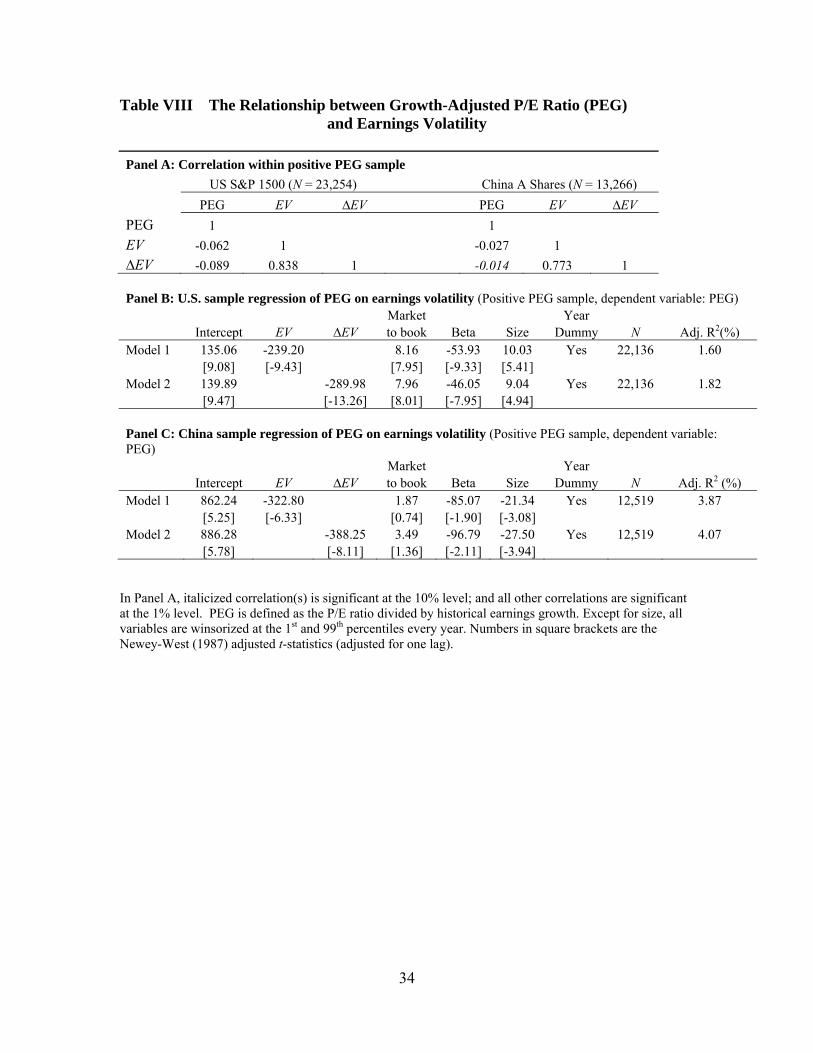
Table VIII shows the relationship between PEG and earnings volatility for the positive
PEG observations. Panel A first shows that the unconditional correlation between PEG and
earnings volatility are still negative for both the U.S. and China. Panels B and C provide,
respectively, the results of the regression of PEG on earnings volatility for the U.S. and China.
We note that the results on earnings volatility are consistent with those using the P/E ratio. That is,
earnings volatility is negatively related to PEG in both the U.S. and China, and the sensitivity of
PEG to earnings volatility in China is larger than in the U.S.
[Table VIII about here.]
4.2 Using Trailing 12-Month Earnings to Calculate P/E
Earlier we use the average earnings of the past three years to calculate the P/E ratio in
order to match the time horizon in our earnings volatility measure. The literature, however,
typically focuses on either trailing 12-month earnings or 12-month forecast earnings. For example,
Ohlson, and Juettner-Nauroth (2005) develop a general model relating price per share to, among
other variables, next year’s expected earnings per share. Since earnings forecasts are generally
not available for Chinese firms in our sample period, as a robustness check, we use the traditional
12-month trailing earnings to calculate P/E instead. The results are shown in Panel A, Table IX.
We find that earnings volatility, measured as either EV or ∆EV, is still significantly negatively
associated with P/E for both the U.S. and China samples under the same set of control variables.
Based on this evidence, we conclude that our results are robust to using trailing 12-month
earnings in the P/E calculation.
[Table IX about here.]

22
4.3 The Small Denominator Problem in the P/E ratio
Earlier we show that our calculation of P/E may suffer from the small denominator
problem when earnings are small, which results in outliers in the dependent variable, the P/E ratio.
Although we winsorize P/E at the 1st and 99th percentiles every year, such a winsorization may
not be sufficient. For example, the maximum P/E ratio in the China sample after the
winsorization is still very large at 1,328.77. We use two ways to address this problem. In the first
instance, we restrict the U.S. (China) sample to EPS no smaller than 0.10 USD (Yuan). In the
second instance, we transform both the P/E ratio (the dependent variable) and earnings volatility
(the independent variable of interest) to percentile ranking valued from 1 to 100 every year. The
results are presented in Panels B and C of Table IX, respectively. We note that all of our
conclusions remain unchanged. In particular, earnings volatility is still negatively related to P/E,
and the sensitivity of P/E to earnings volatility in China is much larger than that in the U.S.
4.3 Scalar Used to Calculate Earnings Volatility
To control for the scalar effect in the calculation of earnings volatility, earlier we use
book equity to deflate earnings. It is possible that our results are driven by the denominator (book
equity) rather than by the numerator (unscaled earnings). To address the potential scalar problem,
we use total assets as an alternative scalar. The results are presented in Panel D, Table IX. None
of our conclusions is changed in this case.
4.4 Controlling for Long-Term Interest Rate
The discounted cash flow model, as well as the “Fed model” discussed earlier, predicts a
negative relationship between P/E and long-term interest rate. Using the 10-year Treasury bond
yield for the U.S. long-term interest rate and over-5-year interest rate of the People’s Bank of
China for the Chinese long-term interest rate, Panel E of Table IX presents the results with

23
interest rate as an additional control variable.14 We note the earnings volatility effect is still very
strong for both the U.S. and China after controlling for long-term interest rate. Compared with the
results that do not control for long-term interest rate (Models 3 and 4 of Table VI), the
magnitudes of coefficient estimates on both EV and ∆EV are actually larger for both China and
the U.S. As such, controlling for long-term interest rate does not alter our conclusions.
4.5 Earnings Comparability between the U.S. and China
The comparison of P/E ratio relies on earnings comparability. Earnings incomparability,
on the other hand, mostly comes from the differences between the U.S. Generally Accepted
Accounting Principles (GAAP) and the Chinese GAAP, of which one key component is when
realized economic profits are reported as earnings (time-shifting of earnings). Consequently,
normalized earnings volatility or cashflow volatility will control for the variation in accounting
methods, as these volatilities directly measure the time-shifting of reported earnings. Our paper
employs earnings volatility, and therefore addresses, at least in part, the earnings comparability
issue.
The concern for earnings comparability is further ameliorated by the harmonization of
accounting standards of the two countries. During our sample period, China had made substantial
progress in bringing its accounting standards on par with the international standards. Two major
pieces of Chinese legislation that cover our sample period are the Accounting Regulation for
Listed Companies, effective from 1998, and the Accounting Standards for Business Enterprise,
14 We do not include year dummies in the regressions in Panel D. Earlier when we used year dummies in
the regressions, we implicitly assumed that year dummies are used to capture macroeconomic variations
across year. Since long-term interest rate is a macroeconomic variable, inclusion of it may no longer
require year dummies in the regression.
24
effective from 2007.15 The former aims at harmonizing the Chinese GAAP with International
Accounting Standards (IAS), and the latter aims at converging China’s accounting standards with
IAS’s International Financial Reporting Standards (IFRS) 2005, which the U.S. Securities and
Exchange Commission is actively considering to adopt for its public firms.16 The converging of
accounting standards across the two countries improves the comparability of reported accounting
numbers. Despite the progress of the Chinese accounting standards, an important caveat remains
that other institutional differences between the two countries such as legal framework, share
capital structure, and corporate governance may weaken the comparability of earnings between
the two countries. Addressing the impact of these institutional differences on the P/E ratio is
beyond the scope of this paper.
5. Concluding Remarks
In this paper, we provide a simple and intuitive explanation as to why the Chinese
markets have a P/E ratio comparable to or only marginally higher than that of the U.S. markets.
We argue that earnings volatility has a countervailing effect against growth rate on the P/E ratio.
While a higher growth rate implies a higher P/E ratio, higher earnings volatility leads to a lower
P/E ratio. We verify the existence of a strong and robust negative P/E-earnings volatility
relationship across a number of measures and model specifications in both countries. Furthermore,
compared with the U.S., China exhibits not only larger earnings volatility but also a higher
sensitivity of P/E to earnings volatility, resulting in a much larger portion of the P/E ratio
negatively affected by earnings volatility. We estimate that earnings volatility explains a
difference in the order of six in the P/E ratio between these two countries, making China’s P/E
ratio much closer to what is observed empirically than otherwise implied by the growth rate of its
macro-economy.
15 Street and Gray (1999), among others, provide evidence on the progress of harmonization. 16 See the following webpage: http://www.sec.gov/rules/other/2010/33-9109.pdf.

25
References:
Allayannis, G. and P. Simko, 2009. Earnings smoothing, analyst following, and firm value,
working paper, University of Virginia.
Chan, K., A. J. Menkveld and Z. Yang, 2008. Information asymmetry and asset prices: Evidence
from the China foreign share discount, Journal of Finance 63, 159-196.
Cheng, P., W. Aerts and A. Jorissen, 2010. Earnings management, asset restructuring, and the
threat of exchange delisting in an earnings-based regulatory regime, Corporate Governance: An
International Review18, 438–456.
Easton, P., 2004. PE ratios, PEG ratios, and estimating the implied expected rate of return on
equity capital, The Accounting Review 79, 73-95.
Huang, A. G., and H. Fung, 2005. Floating the non-floatables in China's stock market: Theory
and design, Emerging Markets Finance and Trade 41, 6-26.
Jiang, G. and H. Wang, 2008. Should earnings thresholds be used as delisting criteria in stock
market? Journal of Accounting and Public Policy 27, 409-419.
Gaver, J. J., and K.M. Gaver, 1993. Additional evidence on the association between the
investment opportunity set and corporate financing, dividend, and compensation policies, Journal
of Accounting and Economics 16, 125-160.
Hunt, A., S. E. Moyer, and T. Shelvin, 2005. Earnings volatility, earnings management, and
equity value, working paper, University of Washington.
Kane, A., A. J. Marcus, and J. Noh, 1996. The P/E multiple and market volatility,
Financial Analysts Journal 52, 16-24.
Lander, J., A. Orphanides, and M. Douvogiannis, 1997. Earnings, forecasts and the predictability
of stock returns: Evidence from trading the S&P, Journal of Portfolio Management 23, 24-35.

26
Newey, W. K., and K. D. West, 1987. A simple, positive semi-definite, heteroskedasticity and
autocorrelation consistent covariance matrix, Econometrica 55, 703-708.
Nikbakht, E., and C. Polat, 1998, A global perspective of P/E ratio determinants: the case of
ADRS, Global Finance Journal 9, 253-267.
Ohlson, J. A., and B.E. Juettner-Nauroth, 2005. Expected EPS and EPS growth as determinants of
value, Review of Accounting Studies 10, 349-365.
Ritter, J., 2005. Economic growth and equity returns, Pacific-Basin Finance Journal 13, 489-503.
Rountree, B., J. Weston, and G. Allayannis, 2008. Do investors value smooth performance?
Journal of Financial Economics 90, 237–251.
Street, D. L., and S. J. Gray, 1999. How wide is the gap between IASC and U.S. GAAP? Impact
of the IASC comparability project and recent international developments. Journal of
International Accounting, Auditing & Taxation 8, 133-164.
Thomas, J. K., and H. Zhang, 2007, Another look at P/E ratios, working paper, Yale University.
Zarowin, P. 1990. What determines earnings-price ratios: revisited. Journal of Accounting,
Auditing, and Finance 5, 439-57.

27
Table I The Number of Sample Firms in the Chinese Markets between 1997 and 2007
Year N 1997 642 1998 745 1999 841 2000 974 2001 1,048 2002 1,108 2003 1,173 2004 1,263 2005 1,268 2006 1,304 2007 1,397
The sample firms exclude firms whose share capital structure includes B-shares.
28
Table II The Market-wide P/E Ratio of U.S. and China
Panel A: Market-wide P/E (Jan. 1997-Dec. 2007) Mean Median Std Min Max
U.S. S&P 1500 20.81 19.83 3.58 15.70 28.45
China 25.03 24.46 12.15 8.84 57.70
Panel B: T-Test of Means
1. China’s P/E is equal to U.S. P/E [4.93]
2. China’s P/E is equal to 110% of the U.S. P/E [2.54]
3. China’s P/E is equal to 120% of the U.S. P/E [0.06]
The market-wide P/E ratio is defined as the sum of market capitalization dividend by the sum of earnings at the monthly frequency, with all of the negative-earnings observations removed. The data for the U.S. is from the Compustat and CRSP, and the data for China is from the CSMAR.
29
Table III Firm-level P/E Ratio Comparison
Panel A: Summary statistics
Equal-wtd. Value-wtd.
N mean mean Median Std Min Max
US, full sample 28,691 27.37 34.38 21.39 48.96 2.19 465.36
US, EPS ≥ $ 0.10 sample 26,914 24.20 28.14 21.04 18.49 2.19 99.98
US, PE ≤ 100 sample 27,586 24.09 28.11 21.05 18.93 2.19 99.98
China, full sample 16,527 41.70 38.41 33.34 130.73 1.04 1,328.77
China, EPS ≥ 0.10 Yuan sample 12,285 32.83 32.68 30.04 25.40 1.04 99.94
China, PE ≤ 100 sample 15,315 32.44 32.70 31.05 29.15 1.04 99.94
Panel B: Annual Cross-Sectional Means
Full sample EPS ≥ 0.10 Sample PE ≤ 100 Sample
Year US China US China US China
1997 26.48 32.84 25.71 28.70 25.65 28.82
1998 29.75 41.14 26.10 33.98 26.05 34.75
1999 28.63 40.91 23.84 35.41 23.70 33.89
2000 33.45 40.84 22.60 43.19 22.46 39.56
2001 26.91 52.06 24.62 46.72 24.48 46.44
2002 25.04 49.35 22.74 37.99 22.84 38.92
2003 25.26 40.24 22.64 30.01 22.48 30.67
2004 27.15 35.87 24.49 24.94 24.08 25.56
2005 27.31 20.50 24.96 17.79 24.91 19.38
2006 25.83 34.64 24.27 24.41 24.21 25.34
2007 24.91 64.34 24.08 43.71 24.01 42.24
T-Test of Annual Cross-sectional Means
The ratio of China's P/E to U.S. P/E is equal to: Full sample EPS ≥ 0.10 Sample PE ≤ 100 Sample
1. 100% [3.77] [3.17] [3.54]
2. 110% [3.00] [2.32] [2.60]
3. 120% [2.24] [1.48] [1.66]
4. 130% [1.49] [0.65] [0.73]
This table is based on interim data (half-year frequency) for the U.S. S&P1500 firms and all Chinese firms over the period of 1997-2007. The data is restricted to positive P/E firm-year observations. PE is the market equity at the end of accounting period divided by average 12-month trailing earnings of the past three years. The “EPS ≥ 0.10 Sample” refers to the firm-halfyear observations that have EPS no smaller than 0.10 dollar (Yuan) for the US (China) sample.

30
Table IV Summary Statistics of Firm-level P/E Ratio, Earnings Volatility, and Control Variables
Panel A: U.S. summary statistics
N MeanStandard deviation
25th percentile Median
75th percentile
EV 28,690 0.05 0.10 0.01 0.026 0.05 ∆EV 28,642 0.06 0.10 0.01 0.030 0.06 EPS growth 28,713 0.12 2.01 -0.04 0.14 0.35 Market to book 28,662 3.34 3.13 1.67 2.42 3.82 Beta 27,344 0.93 0.45 0.61 0.86 1.17 Size (log of million USD) 28,756 7.72 1.50 6.62 7.53 8.67 Panel B: China summary statistics
N MeanStandard deviation
25th percentile Median
75th percentile
EV 16,527 0.09 0.20 0.01 0.026 0.06 ∆EV 15,375 0.10 0.17 0.02 0.034 0.10 EPS growth 16,116 0.12 2.42 -0.14 0.13 0.45 Market to book 17,299 3.89 3.00 1.97 3.10 4.85 Beta 15,374 0.51 0.21 0.35 0.47 0.69 Size (log of CNY) 17,302 21.64 0.92 21.02 21.54 22.11 Size (log of million USD) 17,302 5.72 0.92 5.11 5.62 6.19 Panel C: Percentage of firm-halfyears that have an EPS growth greater than a threshold
Percentage of observations t-stat. of
EPS growth China US Difference difference
≥ 10% 55.2% 59.1% -3.9% [-7.57] ≥ 20% 44.2% 41.7% 2.5% [4.84] ≥ 30% 35.2% 29.5% 5.7% [11.65] ≥ 40% 28.0% 22.1% 5.9% [12.88] ≥ 50% 22.8% 17.7% 5.2% [12.22] ≥ 60% 18.8% 14.7% 4.1% [10.42] ≥ 70% 15.9% 12.6% 3.3% [8.98] ≥ 80% 13.8% 11.1% 2.7% [7.87] ≥ 90% 11.9% 9.8% 2.1% [6.39] ≥ 100% 10.3% 8.9% 1.4% [4.66]
EV (∆EV) is the standard deviation of earnings (year-over-year change in earnings) to book equity over the past three years. EPS growth is measured as the mean year-over-year EPS growth rate over the past three years. Market to book is measured as market equity to book equity. Beta is measured as the stock’s historical beta using the past three-year’s monthly returns. Size is measured as the logarithm of market value of equity. To express the size of Chinese firms in USD, we use the mean exchange ratio of 8.185 CNY/USD during the sample period. Except for size, all variables are winsorized at the 1st and 99th percentiles every year.

31
Table V Sample Correlation between Earnings Volatility and P/E Ratio
Panel A: Interim Data: 1997-2007
US S&P 1500 (N = 28,556) China A Shares (N = 15,375) PE EV ∆EV PE EV ∆EV
PE 1 1
EV -0.049 1 -0.077 1
∆EV -0.058 0.826 1 -0.079 0.752 1
Panel B: Quarterly Data: 2003:Q2-2007:Q4
US S&P 1500 (N = 24,811) China A Shares (N = 10,806) PE EV ∆EV PE EV ∆EV
PE 1 1
EV -0.077 1 -0.111 1
∆EV -0.085 0.843 1 -0.130 0.767 1 This table shows the correlation between the P/E ratio and earnings volatility of the Chinese and U.S. firms. All correlations are significant at the 1% level. PE is defined as market equity at the end of accounting period divided by average 12-month trailing earnings of the past three years. EV (∆EV) is the standard deviation of earnings (year-over-year change in earnings either at quarterly or half-year frequency) to book equity over the past three years.

32
Table VI Regression of P/E on Earnings Volatility
Dependent variable: P/E ratio
Panel A: U.S.
EPS Market Year Adj.
Intercept EV ∆EV Growth to book Beta Size Dummy N R2(%)
Model 1 28.66 -24.62 0.08 No 27,107 0.22
[88.39] [-5.62] [0.77]
Model 2 28.94 -25.43 0.03 No 27,107 0.27
[87.71] [-5.27] [0.12]
Model 3 11.72 -59.68 -0.13 3.7 9.72 -0.35 No 27,107 6.47
[6.61] [-11.46] [-0.49] [16.65] [10.32] [-1.49]
Model 4 11.76 -54.53 -0.21 3.56 10.68 -0.38 No 27,107 6.4
[6.64] [-10.84] [-0.81] [16.45] [11.33] [-1.62]
Model 5 7.30 -60.97 -0.13 3.57 12.35 -0.11 Yes 27,107 6.85
[3.40] [-11.63] [-0.49] [16.58] [11.25] [-0.47]
Model 6 7.25 -57.18 -0.22 3.43 13.55 -0.13 Yes 27,107 6.84
[3.37] [-11.26] [-0.84] [16.42] [12.33] [-0.56]
Panel B: China
EPS Market Year Adj.
Intercept EV ∆EV Growth to book Beta Size Dummy N R2 (%)
Model 1 46.07 -55.41 3.07 No 15,229 0.9
[38.13] [-12.00] [3.39]
Model 2 47.06 -58.24 2.92 No 15,229 0.89
[39.94] [-10.39] [3.22]
Model 3 50.44 -63.97 3.21 4.34 11.47 -1.20 No 15,229 1.73
[1.89] [-12.43] [3.53] [4.66] [2.06] [-0.96]
Model 4 56.39 -78.57 3.02 4.97 11.61 -1.49 No 15,229 1.93
[2.12] [-12.18] [3.32] [5.22] [2.12] [-1.18]
Model 5 137.01 -101.58 3.01 3.78 34.75 -3.17 Yes 15,229 2.51
[4.90] [-13.65] [3.32] [3.87] [4.45] [-2.44]
Model 6 107.6 -94.34 2.89 4.18 35.49 -3.75 Yes 15,229 2.46
[3.87] [-12.39] [3.17] [4.21] [4.59] [-2.87] EPS growth is measured as the mean year-over-year EPS growth rate over the past three years. Market to book is measured as market equity to book equity. Beta is measured as the stock’s historical beta using the past three-year’s monthly returns. Size is measured as the logarithm of market value of equity. Except for size, all variables are winsorized at the 1st and 99th percentiles every year. Numbers in square brackets are the Newey-West (1987) adjusted t-statistics (adjusted for one lag).

Table VII Pooled Regressions for the Relationship between P/E and Earnings Volatility
EV× ∆EV × EPS Market Year Adj. R2
Intercept EV ChinaDummy ∆EV ChinaDummy growth to book Beta Size Dummy N (%)
Model 1 35.27 -49.62 -86.15 0.61 No 42,346 0.90
[77.81] [-10.20] [-4.59] [1.60]
Model 2 34.79 -47.48 -21.06 0.61 No 42,346 0.61
[76.92] [-9.48] [-1.93] [1.57]
Model 3 43.49 -85.27 -138.60 0.57 4.68 3.32 -3.47 No 42,346 3.92
[19.07] [-13.10] [-6.72] [1.41] [13.85] [3.06] [-10.80]
Model 4 38.98 -73.61 -29.79 0.57 4.42 5.01 -3.01 No 42,346 3.24
[17.84] [-12.80] [-2.31] [1.41] [13.35] [4.67] [-9.58]
Model 5 29.82 -51.61 -89.13 0.62 Yes 42,346 1.22
[27.72] [-10.70] [-4.70] [1.61]
Model 6 30.28 -50.40 -18.01 0.59 Yes 42,346 0.89
[28.03] [-10.10] [-1.84] [1.54]
Model 7 36.29 -85.80 -142.47 0.57 4.62 5.09 -3.52 Yes 42,346 4.10
[14.68] [-13.40] [-6.79] [1.43] [13.82] [4.23] [-11.10]
Model 8 32.43 -76.14 -30.02 0.57 4.33 7.48 -3.10 Yes 42,346 3.47
[13.46] [-13.40] [-2.32] [1.40] [13.22] [6.28] [-9.90] This table pools the US and China samples and estimates a single regression. The dependent variable is P/E, measured as the market equity at the end of accounting period divided by average 12-month trailing earnings of the past three years. EV (∆EV) is the standard deviation of earnings (year-over-year change in earnings) to book equity over the past three years. EPS growth is measured as the mean year-over-year EPS growth rate over the past three years. Market to book is measured as market equity to book equity. Beta is measured as the stock’s historical beta using the past three-year’s monthly returns. Size is measured as the logarithm of market value of equity. To express the size of Chinese firms in USD, we use the mean exchange ratio of 8.185 CNY/USD during the sample period. ChinaDummy is dummy variable that equals 1 if the observation is from the China sample and 0 otherwise. Except for size, all variables are winsorized at the 1st and 99th percentiles every year. Numbers in square brackets are the Newey-West (1987) adjusted t-statistics (adjusted for one lag).
34
Table VIII The Relationship between Growth-Adjusted P/E Ratio (PEG) and Earnings Volatility
Panel A: Correlation within positive PEG sample
US S&P 1500 (N = 23,254) China A Shares (N = 13,266)
PEG EV ∆EV PEG EV ∆EV
PEG 1 1
EV -0.062 1 -0.027 1
∆EV -0.089 0.838 1 -0.014 0.773 1 Panel B: U.S. sample regression of PEG on earnings volatility (Positive PEG sample, dependent variable: PEG) Market Year Intercept EV ∆EV to book Beta Size Dummy N Adj. R2(%) Model 1 135.06 -239.20 8.16 -53.93 10.03 Yes 22,136 1.60 [9.08] [-9.43] [7.95] [-9.33] [5.41] Model 2 139.89 -289.98 7.96 -46.05 9.04 Yes 22,136 1.82 [9.47] [-13.26] [8.01] [-7.95] [4.94] Panel C: China sample regression of PEG on earnings volatility (Positive PEG sample, dependent variable: PEG) Market Year Intercept EV ∆EV to book Beta Size Dummy N Adj. R2 (%) Model 1 862.24 -322.80 1.87 -85.07 -21.34 Yes 12,519 3.87 [5.25] [-6.33] [0.74] [-1.90] [-3.08] Model 2 886.28 -388.25 3.49 -96.79 -27.50 Yes 12,519 4.07 [5.78] [-8.11] [1.36] [-2.11] [-3.94]
In Panel A, italicized correlation(s) is significant at the 10% level; and all other correlations are significant at the 1% level. PEG is defined as the P/E ratio divided by historical earnings growth. Except for size, all variables are winsorized at the 1st and 99th percentiles every year. Numbers in square brackets are the Newey-West (1987) adjusted t-statistics (adjusted for one lag).

35
Table IX Robustness Checks
Panel A: Using trailing 12-month earnings instead of average earnings of the past three years for P/E ratio
EPS Market Year Adj. R2
Intercept EV ∆EV growth to book Beta Size Dummy N (%)
U.S. 17.68 -8.40 -0.34 2.03 17.63 -1.26 Yes 27,108 6.97
[10.58] [-3.09] [-1.22] [13.52] [21.20] [-6.69]
16.94 -6.94 -0.37 1.92 17.50 -1.17 Yes 27,107 6.94
[10.13] [-3.53] [-1.36] [13.01] [20.81] [-6.23]
China 138.96 -19.28 5.26 9.23 18.22 -24.62 Yes 15,370 7.92
[18.28] [-3.37] [7.58] [12.00] [2.26] [-17.81]
132.56 -16.72 5.19 9.02 19.13 -24.38 Yes 15,229 7.92
[17.16] [-3.17] [7.47] [11.57] [2.23] [-17.63]
Panel B: Restricting to EPS-no-smaller-than-0.1 sample
EPS Market Year Adj. R2
Intercept EV ∆EV growth to book Beta Size Dummy N (%)
U.S. 7.18 -48.42 -0.34 3.55 13.11 -0.15 Yes 26,647 7.50
[3.48] [-11.10] [-1.41] [16.77] [12.37] [-0.67]
7.06 -44.62 -0.43 3.41 14.26 -0.16 Yes 26,647 7.46
[3.42] [-10.54] [-1.66] [16.57] [13.47] [-0.72]
China 85.17 -77.81 2.16 3.15 15.22 -1.13 Yes 12,196 2.69
[3.63] [-11.11] [1.88] [3.21] [2.30] [-0.99]
61.20 -76.88 2.08 3.46 15.81 -1.49 Yes 12,196 2.69
[2.57] [-10.63] [1.81] [3.50] [2.37] [-1.31]
Panel C: Using P/E and earnings volatility percentile rankings instead of values in regressions
EPS Market Year Adj. R2
Intercept EV ∆EV growth to book Beta Size Dummy N (%)
U.S. 28.42 -0.08 -0.17 2.99 11.67 -0.53 Yes 27,107 15.02
[21.67] [-11.00] [-1.37] [28.93] [21.37] [-2.34]
26.84 -0.05 -0.15 2.88 11.53 -0.60 Yes 27,107 14.63
[20.61] [-6.86] [-1.26] [28.19] [20.79] [-2.80]
China 132.36 -0.34 0.91 3.59 14.65 -3.91 Yes 15,229 17.82
[19.14] [-36.42] [6.55] [19.26] [7.21] [-12.00]
132.71 -0.26 0.92 3.35 16.28 -4.09 Yes 15,229 13.32
[18.54] [-27.12] [6.46] [17.97] [7.67] [-12.17]
Panel D: Using ROA instead of ROE to calculate earnings volatility
EPS Market Year Adj. R2
Intercept EV ∆EV growth to book Beta Size Dummy N (%)
U.S. 6.67 -135.54 -0.08 3.16 13.89 -0.07 Yes 27,107 5.87
[3.01] [-4.26] [-0.29] [15.25] [12.45] [-0.31]
6.47 -109.09 -0.12 3.14 14.38 -0.10 Yes 27,107 5.93
[2.98] [-5.13] [-0.46] [15.14] [12.91] [-0.44]
China 127.57 -185.78 3.11 3.35 32.14 -2.79 Yes 15,370 2.19
[4.58] [-12.98] [3.43] [3.47] [4.17] [-2.15]
91.56 -172.26 3.04 3.51 33.62 -2.93 Yes 15,229 2.06
[3.30] [-11.18] [3.34] [3.57] [4.37] [-2.25]

36
Panel E: Controlling for long-term interest rate
Interest EPS Market Year Adj. R2
Intercept EV ∆EV rate growth to book Beta Size Dummy N (%)
U.S. 11.71 -61.24 -3.52 -0.14 3.82 9.77 -0.42 No 27,107 6.67
[6.83] [-12.38] [-2.45] [-0.56] [17.67] [10.94] [-1.83]
11.68 -55.54 -3.75 -0.22 3.67 10.76 -0.43 No 27,107 6.58
[6.81] [-11.50] [-2.61] [-0.89] [17.40] [12.05] [-1.92]
China 27.82 -81.94 3.03 3.07 4.14 8.43 -2.01 No 15,229 1.95
[1.01] [-13.53] [2.95] [3.44] [4.55] [1.86] [-1.62]
45.42 -80.47 2.40 2.96 4.88 10.28 -1.65 No 15,229 1.96
[1.63] [-12.41] [2.67] [3.31] [5.22] [2.01] [-1.31]
This table provides various robustness checks for the main regressions of Table VI. All variables are the same as Table VI unless otherwise specified. In Panel A, the dependent variable of P/E ratio is defined as the market equity at the end of accounting period divided by the 12-month trailing earnings. In Panel B, the U.S. (China) sample is restricted to EPS no smaller than 0.10 USD (Yuan). In Panel C, P/E and EV (∆EV) is defined as the percentile ranking, valued from 1 to 100, of their raw counterparts every year. In Panel D, EV (∆EV) is the standard deviation of earnings (year-over-year change in earnings) to total assets over the past three years. In Panel E, interest rate for the U.S. sample is the 10-year Treasury bond yield from the St. Louis Federal Reserve and for the China sample is the over-5-year interest rate from the People’s Bank of China. Numbers in square brackets are the Newey-West (1987) adjusted t-statistics (adjusted for one lag).

PE
0
10
20
30
40
50
60
Year97 98 99 00 01 02 03 04 05 06 07 08
PE Ratio: China US
Figure 1: The Market-wide P/E Ratio for the U.S. and China. The market-wide P/Eratio is defined as the sum of market capitalization dividend by the sum of earnings.
37

%
3
4
5
6
7
8
9
10
11
12
13
14
15
16
Jan. 97 to Dec. 0797 98 99 00 01 02 03 04 05 06 07 08
Monthly interest rate: China (over-5-year) US (10-year Treasury yield)
Figure 2: Long-term interest rates of the U.S. and China. The U.S. long-term interest rateis 10-year Treasury yield, and the long-term interest rate of China is the over-5-year interest ratepublished by the People’s Bank of China (the Chinese central bank).
38

0.04
0.05
0.06
0.07
0.08
0.09
0.10
0.11
0.12
Year1997 1998 1999 2000 2001 2002 2003 2004 2005 2006 2007
EV: Std Mean
(a) US’s EV
0.04
0.05
0.06
0.07
0.08
0.09
0.10
0.11
0.12
0.13
Year1997 1998 1999 2000 2001 2002 2003 2004 2005 2006 2007
Delta EV: Std Mean
(b) US’s ∆ EV
0.0
0.1
0.2
0.3
0.4
0.5
0.6
Year1997 1998 1999 2000 2001 2002 2003 2004 2005 2006 2007
EV: Std Mean
(c) China’s EV
0.040.060.080.100.120.140.160.180.200.220.240.260.280.300.320.340.360.380.400.42
Year1997 1998 1999 2000 2001 2002 2003 2004 2005 2006 2007
Delta EV: Std Mean
(d) China’s ∆ EV
Figure 3: Time-series of P/E ratio and earnings volatility. This figure plots the annualcross-sectional means of P/E, EV, and ∆EV of the U.S. sample (Panels (a) and (b)) and the Chinasample (Panels (c) and (d)). The dotted solid line shows the mean, and the gray bar shows thestandard deviation.
39

Mean = 0.12Median = 0.14Min. = -15.28Max. = 13.95Skewness = 0.59Kurtosis = 23.81
(a) US EPS Growth Distribution
Mean = 0.12Median = 0.13Min. = -18.76Max. = 19.49Skewness = -0.94Kurtosis = 33.53
(b) China EPS Growth Distribution
Figure 4: Histogram of EPS growth. This figure plots the histogram, truncated between −2and 2 and expressed as percentage, of EPS growth of the U.S. sample (Panel (a)) and the Chinasample (Panel (b)). The text box in each panel shows the distribution statistics of the EPS growth.
40