laser light scattering || methods of data analysis

V I I METHODS OF DATA

ANALYSIS

7 .1 . NATURE OF THE PROBLEM For a polydisperse system of particles in suspension (or macromolecules in

solution), the first-order electric field time correlation function g{1)

(τ) is related to the characteristics linewidth (Γ) distribution function G(T) through a Laplace transform relation:

g{%) = | °° G(r )e -

rMr, (7.1.1)

where τ denotes the delay time. g{i) (τ) is measured and known. G(T) is the

unknown characteristic linewidth distribution function, which we want to determine. Solving for G(F) from Eq. (7.1.1), either analytically or numerically, is known as Laplace inversion and is the main subject of this chapter. The recovery of G(T) from g

a) (τ) using data that contains noise is an ill-posed

problem. A correlator has a finite delay-time increment Δτ and contains a finite number Ν of delay-time (τ) channels, whether equally or logarithmically spaced in delay time; e.g., a correlator can cover a finite range of delay times w i t h i m in ~ A i , i m a x( ^ τΝ) = Ν Δτ for an equally spaced delay-time correlator, implying that the integration limits of Eq. (7.1.1) cover from r m in to T m ax instead of 0 to oo . Therefore, g

(1) (τ) is bandwidth-limited. The above

illustrations tell us that the measured data g{1) (τ) contains noise and is

243

2 4 4 METHODS OF DATA ANALYSIS CHAPTER VII

bandwidth limited. What the correlator measures is in fact an estimate of the correlation function, i.e., it is a time-averaged time correlation function, measured using the usual optical arrangements that we have discussed in previous chapters (e.g., see Chapter 6).

The ill-conditioned nature of Laplace-transform inversion suggests that we should try to measure the intensity time correlation function G

( 2) (τ) to a high

level of precision (low noise) and over a broad range of delay time (decreasing the bandwidth limitation, which is governed by the unknown G(F)) before we attempt to perform the Laplace-transform inversion according to Eq. (7.1.1). The uninitiated reader may immediately wonder what (1) a high level of precision and (2) a broad range of delay time mean. The following discussions and Section 7.3 represent some guidelines to these two conditions.

The noise can come from the photon-counting statistics and the statistical nature of intensity fluctuations (Saleh and Cardoso, 1973). The photodetection noise can be reduced by increasing the total number of counts per delay-time increment. As

G

( 2»(T) = (n(t)n(t + τ)> = Ns<n( i )>

2( l + J %

( 1» ( T ) |

2) , (7 .1 .2)

the magnitude of G( 2)

(τ) is closely related to the background A( = Ns(n(t))2),

i.e., to the total number of samples, Ns, and the mean number of counts per sample time, <n(i)>. Thus, aside from / %

( 1 )( τ ) |

2, the magnitude of the intensity

correlation-function estimate can be increased by increasing the number of samples, N S, i.e., by increasing the measurement time and /or by increasing the incident light intensity. Furthermore, as the photodetection process is uncorrec ted among neighboring channels, there should be a sufficient number of channels in the measured intensity correlation function, allowing better curve fitting through the centroid of the noise fluctuations. However, in the correlated intensity fluctuations, the intensity-fluctuation noise can be reduced only by increasing the measurement time. In any case, we should recognize that the presence of noise cannot be avoided. Indeed, even computer-simulated intensity correlation data contains noise because of roundoff errors in the computer. We wish to obtain an estimate of G(T), having measured an inevitably noisy and incomplete representation of the intensity time correlation function. Due to the ill-conditioning, the amount of information that can be recovered from the data is quite limited, i.e., small errors in the measurement of G

( 2) (τ) can produce very large errors in the reconstruction of G(T).

Attempts to extract too much information result in physically unreasonable solutions. Therefore, a correct inversion of Eq. (7.1.1) must involve some means of limiting the amount of information requested from the problem. In recent years, much attention has been focused on this inversion problem (Bertero et a/., 1984, 1985; Refs. 18-29 of Chu et al, 1985; Livesey et al. 1986; Vansco et a/., 1988; Dhadwal, 1989; Nyeo and Chu, 1989; Langowski and By ran, 1990).

S E C T I O N 7 .2 A S C H E M A T I C O U T L I N E O F T H E P R O C E D U R E 2 4 5

7.2. A SCHEMATIC OUTLINE OF THE PROCEDURE In an ill-conditioned problem, it is important to know that fitting the data

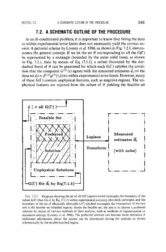
to within experimental error limits does not necessarily yield the correct answer. A pictorial scheme by Livesey et al. 1986, as shown in Fig. 7.2.1, demonstrates the general concept. If we let the set ^ corresponding to all the G(T) be represented by a rectangle (bounded by the outer solid lines), as shown in Fig. 7.2.1, then by means of Eq. (7.1.1), a subset (bounded by the dot-dashed lines) of ^ can be generated for which each G(T) satisfies the condition that the computed G

( 2) (τ) agrees with the measured estimates d{ on the

data set df( = j 81 / 2

l é /( 1 )

( T i ) | ) to within experimental error limits. However, many of these G(T) contain unphysical features, such as negative regions. The un-physical features are rejected from the subset of ^ yielding the feasible set

G [ = a l l G ( T ) }

FIG. 7.2.1 . Diagram showing the set of all G(F) spectra (solid rectangle), the boundary of the subset G(T) that fits dt by Eq. (7 .1 .1) within experimental accuracy (dot-dash rectangle), and the boundary of the set of physically allowable G(T) (dashed rectangle); the intersection of the two sets is the feasible set (stippled region). Inside the feasible set, the aim is to choose a preferred solution by means of various methods of da ta analysis, such as methods of regularization or maximum entropy (Livesey et al. 1 9 8 6 ) . The preferred solution can become more restrictive if additional information about the system can be introduced dur ing the analysis as shown schematically by the double-hatched region.

246 M E T H O D S OF DATA A N A L Y S I S CHAPTER V I I

(stippled region) in which every G(F) yields a computed G( 2)

(τ) in agreement with di and is physically allowable. The various methods of data analysis try to choose a "preferred" solution (hatched region). If additional boundary conditions can be incorporated into the data analysis procedure, a further reduced set of preferred solutions (double-hatched region) can be chosen.

7.3. EXPERIMENTAL CONSIDERATIONS From the discussions in Sections 7.1 and 7.2, it is evident that the measured

estimates dt on the data dt must be treated with care, e.g., dt should cover a range of xt so that T m in and T m ax represent the corresponding values of G

( 2) (τ)

with G(rm a x) ~ 0 and G(Tm i n) ~ 0. In other words, we should cover di so that, as τ ->0, d

2 = β | #

( 1 )( τ ) |

2 -» β. So, we arbitrarily set | #

( 1 )(τ = Δτ ) |

2 ~

0.998. dt must also cover a range of τ such that at T M A X, \g(l) ( i m a x) |

2 < 0.005,

i.e., the agreement between the measured and the computed baseline should agree to within a few tenths of a percent in order to avoid significant distortion of the resultant G(Y) from the Laplace-transform inversion.

In Eq. (7.1.2), the normalization of fef(= G( 2)

(τ^-Λ) by Ns (n(t)}2 suggests

a special importance for the baseline A( = Ns(n(t)}2\ which depends on Ns

and <n(i)> as well as on the delay time over which G( 2)

(τ) is measured, since we want to set G

( 2) (τ = r m a x) close to Ns(n(t)}

2, i.e., to within 0.005β. The

importance of the baseline has been mentioned by many authors (Oliver, 1981; Chu, 1983; Weiner and Tscharnuter, 1985) and treated in a more quantitative manner by Ruf (1989). The relationship between the level of statistical errors in a measured intensity autocorrelation function and the relative size distribution width (uncertainty) has been considered (Kojro, 1990). Errors in the baseline uncertainties play a more complex role than merely shifting g(1) (τ). In addition to covering the proper τ-range and to recognizing the

importance of the baseline before attempting a meaningful data analysis, the statistical errors due to the photodetection process and intensity fluctuations should be minimized by taking short batches of the net intensity correlation function and normalizing the (calculated) baseline for each batch separately (Oliver, 1979); and for long delay times, by considering the difference between <w(i)> and (n(t + τ)>, as has been discussed by Schatzel et al. (1988).

Finally, we must recognize the fact that Eq. (7.1.1) cannot be implemented unless we have good data, i.e., the sample solution must be properly clarified, so that spurious effects, such as contributions due to dust, are absent, and the instrument properly prepared, such that there is no stray light or after pulsing. There is a general saying, "garbage in, garbage out." The ill-conditioning of the Laplace inversion makes data taking especially crucial, as we need very precise data with some ideas on the error limits of our photon correlation measurements in order to reconstruct G(T).

To summarize the experimental conditions for measuring the intensity time correlation function (ICF), we need to consider the following steps.

S E C T I O N 7 .4 B R I E F O U T L I N E O F C U R R E N T D A T A A N A L Y S I S T E C H N I Q U E S 2 4 7

(1) Have a good sample preparation procedure, including clarification of the solution. The presence of foreign particles, such as dust particles, will be reflected in the ICF and consequently G(T). Dust discrimination by electronic means is feasible, provided that one knows the geometry of the scattering volume and the size of the dust particles, i.e., the average transit time for the dust particle to pass through the scattering volume. However, it is advisable to start with a clean system in which only the particles (or macromolecules) of interest are present. As dust particles are usually large, even a small number can influence the scattering behavior of smaller particles at small scattering angles. For dust discrimination by electronic means, we monitor the scattered intensity over a short delay-time increment. While allowing for normal intensity fluctuations, one can set a threshold level indicating the entrance of large dust particles into the scattering volume. The correlator is then shut off* electronically for a preset (transition) time before a resumption of operation. The problem with this type of dust discrimination is that it cannot be entirely objective, because we need to know the threshold level and the dust transit time.

(2) Test the correlator over the delay-time range of interest, making sure that afterpulsing and other electronics problems have been eliminated. Afterpulsing is a serious problem for certain types of photomultipliers operating at short delay-time increments ( < 100 nsec).

(3) Measure the I C F over a broad delay-time range such that, e.g.,

(a) d2 = (τ) |

2 -+ β as τ -+ 0, e.g., \g

{1) (τ = Δτ ) |

2 - 0.998,

(b) d, decay to A at τ = T m a x, e.g., ( i m a x) |2 < 0.005.

(4) Have extra channels with long delays to measure the baseline A experimentally. The measured baseline A should agree with the computed baseline A = Ns (n(t))

2 to within a few tenths of a percent.

(5) It is better to take short batches of the net ICF, each of which has been normalized by a separate (calculated) baseline, and then add the net ICFs together.

(6) For long delay times, the averages of <n(i)> and <w(i + τ)> can be different. Thus, one should use <w(i)> + τ)>, not <n(i)>

2, in the baseline

computation.

7.4. BRIEF OUTLINE OF CURRENT DATA ANALYSIS TECHNIQUES

We may subdivide current data analysis techniques into several operational categories:

(1) Cumulant expansion:

1η|0α ,(τ) | = -Ττ+^μ2τ

2 - 1 μ 3τ

3 + · • · , (7.4.1)


where

Γ = J ' r G i n d r , (7.4.2)

μ , = J V - r ) ' G ( r ) d r . (7A3)

The cumulant expansion (Koppel, 1972) is valid for small τ and sufficiently narrow G(F). One should seldom use parameters beyond μ 3, because over-fitting of data with many parameters in a power-series expansion will render all the parameters, including Γ and μ 2, less precise. This expansion has the advantage of getting information on G(T) in terms of f and μ 2 without a priori knowledge of the form of G(r), and is fairly reliable for a variance μ 2/ Γ

2 < 0.3. The cumulant expansion algorithm is fast and easy to implement.

One often uses its results as a starting point for more detailed data analysis. (2) Known G(T): The ill-conditioned nature of Laplace inversion is

essentially removed if the form of G(T) is known. Thus, for known G(T), the problem is not so difficult and will not be discussed here. It is sufficient to say that one can achieve much better results on the parameters of the distribution function G(F) if its form is known.

(3) Double-exponential distribution:

\gW(T)\ = ^ β χ ρ ί - ^ τ ) + , 4 2e x p ( - r 2T ) , (7.4.4)

where A1 + A2 = 1. With the three unknown parameters Γ ΐ9 Γ 2, and Αγ (or A2\ this is a nonlinear least-squares fit to |#

( 1 )(τ) | . If one knows G(T)

to be a bimodal distribution consisting of two ^-functions, Eq. (7.4.4) should be very easy to use. Without knowing the form of G(T), it is still useful to fit fairly broad G(r) distributions (say with μ 2/ Γ

2 < 0.5). Then, the com

puted A{ and T{ values can be used to compute a meaningful average linewidth (Γ) and variance ( μ 2/ Γ

2) with Γ = ΑίΓί + ^42Γ2 and μ 2/ Γ

2 =

(ΑχΓΐ + Α 2Γ 2) / ( Α 1Γ 1 + Α2Γ2)2 — 1. The double-exponential form can

fit \g{1) (τ)I over a broader range of τ than the cumulant expansion for

broader \g{1) (τ)|. However, its application remains limited.

(4) Method of regularization: This is a smoothing technique that tries to overcome the ill-posed nature of the Laplace-transform inversion. The regularized inversion of the Laplace integral equation requires little prior knowledge on the form of G(r). The most tested and well-documented algorithm has been kindly provided by Provencher (1976,1978,1979,1982a, b, c, 1983) to research workers upon request and is known as C O N T I N . The serious worker in the field who wants to determine reliable Γ and μ2 values should learn how to use C O N T I N , which has a detailed set of instructions.

S E C T I O N 7.4 B R I E F O U T L I N E O F C U R R E N T D A T A A N A L Y S I S T E C H N I Q U E S 249

(5) Method of maximum entropy: The method of maximum entropy (MEM) provides the best possibility for future improvement in data analysis. It can proceed from an unbiased, objective viewpoint and permits the introduction of constraints that reflect the physics of the problem of interest.

Unfortunately, inversion of the Laplace integral equation cannot be understood on an elementary mathematical level. Thus, the following discussions (Sections 7.5-7.6) can be skipped by the less mathematically oriented reader. One should learn how to use the cumulant expansion, the double-exponential fit, and C O N T I N , and watch out for the development of the M E M . In the analysis procedure, always try to generate simulated data sets with different noise levels and deUy-time ranges that are comparable to (and broader than) the measured data set, and test the programs in order to gain confidence in their validity. Objectivity is the key. Normally, one should not try to get more than three parameters ( Γ , μ 2, μ 3) from the fitting procedures.

Many data analysis techniques rely on minimizing the sum of the squares of the normalized residuals. We seek solutions to Eq. (7.1.1) that minimize some measure of the discrepancies between the discrete sample data points di and the corresponding values j S

1 / 2| ^

( 1 )( ^ i ) l that can be calculated from Eq. (7.1.1),

subject to the requirement that the solution be well behaved. The minimization of the L

2 norm of residuals (i.e., least-squares minimization) involves

an iteration scheme that aims at descending the χ2 surface to the minimum.

If a G(T) is estimated by simply minimizing χ2, the solution to Eq. (7.1.1)

may be overfitted, resulting in erroneous G(T) even when χ2 can be fitted to

within experimental error limits, as shown schematically by the dot-dashed rectangle in Fig. 7.2.1. The particular solution chosen could also depend on the computer algorithm or be biased by the choice of starting solution.

In order to remove the ill-conditioning, the correct inversion of Eq. (7.1.1) must involve some means to reduce the size of the feasible set, i.e., to reduce the amount of information requested from the problem; this has been done in a number of ways. The more popular ones, though by no means all, are summarized in the following sections. This summary with comments tries to inform the reader what has been accomplished. The cumulant method (Section 7.4.6), the multiexponential singular-value decomposition (Section 7.5), and the maximum-entropy formalism (Section 7.6) are presented in some detail for those readers interested in learning more.

7.4.1. EIGENVALUE DECOMPOSITION Eigenvalue decomposition of the Laplace kernel coupled with reliable

estimates of the noise in the data can be used to recover estimates of G(T) (McWhirter and Pike, 1978). The eigenvalues are shown to decrease rapidly below the noise level of the data, at which point it becomes meaningless to


extract further knowledge about the characteristic linewidth distribution G(r). Unfortunately, it is difficult to formulate a quantitative description of the noise in the data. The discussions in Section 7.3 have treated some aspects of sources of noise in the measured data, and attempts have been made, at least in the first approximation, to incorporate the noise error in the baseline subtraction (Ruf, 1989). Nevertheless, it would be difficult to unambiguously determine the amount of noise in the measured data and so to determine the number of terms that should be retained in the eigenfunction expansion.

By limiting the amount of information in the beginning so that the support of the solution is restricted (between T m in and T m a x, the upper and lower frequencies of the characteristic linewidth distribution) due to a prior knowledge of the spread of molecular sizes (Bertero et. al, 1982, 1984), Pike and his coworkers proposed to use a sufficiently small number Ν of characteristic linewidths in order to digitize G(T) discretely and to ensure uniqueness of the solution.

Two schemes have been suggested by Pike and his coworkers to interpolate the shape of G(T) between the few (N) exponentials permitted by the eigenvalue decomposition techique. Pike et al (1983) proposed an interpolation formula that sets the coefficients of the eigenfunction expansion to zero beyond a cutoff. An alternative solution (Pike, 1981; Ostrowsky et al, 1981) is to phase-shift the transform coefficient.

Bertero et al (1982), for example, have shown that the obtainable resolution is increased as the support ratio γ ( = T m a x/ r m i n) is decreased. It should be noted that T m in and T m ax refer to the bounds of the true distribution. More information on G(T) can be recovered with the introduction of additional physical constraints. Nevertheless, the sharp truncation at T m in and T m ax produces too much sensitivity to the position of Γ ( = $ΓΟ(Γ)άΓ) within the interval from T m in to T m a x, as well as some unphysical edge effects.

In a recent LS polydispersity analysis of molecular diffusion by Laplace-transform inversion in weighted species, Bertero et al (1985) imposed a profile function f0(T) having the measured mean Γ and polydispersity index Q ( = μ 2/ Γ

2) to localize the recovered solution and to improve its resolution.

The profile function is large in the expected region of the solution and tapers off smoothly to zero on either side, so that the integration in Eq. (7.1.1) is no longer restricted to [ T m i n, r m a x] but is returned to [ 0 , o o ] . The problem becomes

J o

where G(T) = /0(Γ)φ(Γ). Bertero et al. (1985) have, for example, chosen a gamma distribution for f0:

ε-Γ%(Γ)φ(Γ)άΓ, (7.4.5)

(7.4.6)


with g m ax = ( μ 2/ Γ2) = 1/B. There is also a lower limit ô m i n, which is

determined empirically. The reader is referred to the original article for details.

7.4.2. SINGULAR-VALUE DECOMPOSITION The singular-value decomposition technique (Golub and Reinsch, 1970;

Hanson, 1971; Lawson and Hanson, 1974) provides a means of determining the information elements of the actual problem (including constraints) by ordering these elements in decreasing importance. It has been applied by Bertero et al. (for example, see 1982). The problem of how many terms to use before cutoff remains. This is, however, one of the simpler methods. So we shall discuss the technique in some detail later (see Section 7.5).

7.4.3. REGULARIZATION METHODS Regularization methods aim at seeking solutions to Eq. (7.1.1) from a class

of functions that make the inversion of the integral equation well behaved. These pseudosolutions generally correspond to solutions of minimum energy, nonnegativity, or some other reasonable physical constraints. A regularizer may be used to restrict the curvature of G(F) in order to give a smoother distribution. By imposing nonnegativity on the G(T) distribution and by choosing the degree of smoothing based on the Fisher test, Provencher (1976, 1978,1979,1982a,b,c, 1983) has made available an automated procedure that combines regularization with the eigenfunction analysis to yield a thoroughly tested solution to Eq. (7.1.1). The C O N T I N program is well documented and widely used, and has been adapted by workers to IBM P C / A T microcomputers. It is also available through Brookhaven Instruments (New York) for the BI correlators (not an endorsement). A simpler version (Chu et al. 1985), based on the procedure by Miller (1970), is limited to mainly unimodal distributions. Provencher's C O N T I N program should be one of the programs at the disposal of the reader who is interested in using quasielastic light scattering for polydispersity analysis.

7.4.4. METHOD OF MAXIMUM ENTROPY (MEM) The method of maximum entropy has been applied to a variety of problems

in image (or structural) analysis. Its application to the reconstruction of G(T) based on the Shannon-Jaynes entropy provides the best introduction of a priori information for the structure of G(r) and has been explored by several authors (Livesey et al. 1986; Vansco et al., 1988; Nyeo and Chu, 1989). A direct comparison of the present-day methods shows that C O N T I N and the M E M yield comparable results (see Section 7.7). It is likely that with additional knowledge of #

( 1 )(τ) , the M E M could be improved further and could yield

somewhat higher resolving power than C O N T I N (Langowski and Bryan, 1990).


7.4.5. EMPIRICAL FORMS FOR G{T) OR | #( 1 )

( τ ) Ι

If for any reason, such as in a polymerization process, we know the form of G(r), then the parameters of G(T) can be determined more precisely because we can introduce the information directly into Eq. (7.1.1). However, if the calculated curve represents only an analytical approximation to the expected curve, the true solution may now be excluded from the feasible or allowed set of solutions. For example, if G(T) is a truncated Gaussian or Pearson curve, we can generate β\g

il)(τi)\

2 in order to compare it with df. A better comparison

can be made if β is known experimentally, instead of as a fitting parameter. The results with known G(T) can still be elusive if there were too many parameters, as in a Pearson's curve ( Chu et al, 1979).

7.4.6. DIRECT INVERSION TECHNIQUES (CHU ETAL, 1985)

Direct inversion techniques, such as calculating the cumulants (Koppel, 1972) or the moments (Isenberg et al 1973) of G(T) are well suited to reasonably narrow, well-behaved characteristic linewidth distribution functions, but have grave difficulties in handling broad ( μ 2/ Γ

2 > 0.3) or multimodal

distributions in G(T). The following paragraphs are transferred with only three minor changes

from Chu et al (1985, pp. 264, 267-269, 278-287). G(T) is described in terms of a moment expansion:

1η|</( 1 )

(τ)| = - Γτ + ^ μ 2τ2 - ^ μ 3τ

3 + ^ ( μ 4 - 3 μ 2) τ

4

(7.4.1)

where Km(F) is the rath cumulant. Kx = μι = 0, Κ2 = μ2, Κ3 = μ3, and Κ4. = μ4. — 3μ2. One can fit this directly to the measured quantity b( ( = G

( 2 )( T J ) — A), recognizing that a constant (Αβ)

1/2 will be added to

Eq. (7.4.1). Note that Αβ (not A) is an adjustable parameter that will be determined by the algorithm as presented here. This is a straightforward weighted linear least-squares problem, the weighting factors being necessary because the operation of taking the logarithm of the data has affected the (approximately) equal weighting of the data points. In fact, the data points are not equally significant. Jakeman et al (1971) have derived expressions for the variance of the correlation function as a function of delay channel, but only in the limit of single-exponential decays. If we assume that the major source of statistical uncertainty is counting statistics, and that the errors in adjacent channels are uncorrelated, we conclude that the error in a particular channel ought to be approximately constant, since the first channel (with the maximum in the


correlation function) rarely differs by more than 40% from the last. If we introduce a weighting of each data point by another factor corresponding to ft I"

1, additional complications may result, as the net value of the data points

becomes very small near i m a x. Alternatively, we can use the net autocorrelation function directly (after subtracting the baseline) and fit to

ft,- = 4/? exp ι - 1 , 1 , 2( - Γ ι , - + - μ 2τ ,

2- - μ 3τ ,

3 + (7.4.7)

We introduce ft, to distinguish the data vector of this problem from that of ft,. The least-squares problem is a nonlinear one, but has the advantage that the relative statistical weighting of the data is unaffected. For the implementation of the nonlinear least-squares algorithm we have in this case the parameter vector Ρ defined by

Pi = *β,

P2 = Γ, (7.4.8)

P , . , .>2 = K , ( r ) / ( j - 1)!.

The χ2 surface is defined by the value of the sum of the squares of the residuals

with M being the number of delay channels (i.e., data points), M ^ Σ Ι > . - / ( τ ;, Ρ ) ]

2,

i= 1 at the point located by the vector Ρ = ( P l 5P 2, . . . , P n) , with /(τ,·;Ρ) being the value of ft,- calculated from the model at the point τ, where the parameters of the model have the values given by the vector P. Therefore, an initial estimate of Ρ is supplied to the routine (i.e., a starting point at which to evaluate the χ

2

surface), and an appropriate algorithm is used to choose the direction of descent (i.e., to find some suitable modification to Ρ so as to reduce χ

2). Three

methods are in common use. They are the gradient method, the G a u s s -Newton method, and the Levenberg-Marquard t method. Interested readers should refer to Chu et al (1985) and the original references for details.

Eq. (7.4.7) becomes

S, = Λ exp[2( - Ρ 2τ ; + Ρ3τ? - Ρ4τ? + · · · )] , (7.4.9)

and the elements of the Jacobian matrix are

Jn = - β χ ρ [ 2 ( - Ρ 2τ , + Ρ3τ? - Ρ4τ? + · · ·)] = - e x p ( Z ) ,

Jii = 2Ρ1τ,εχρ(Ζ),

Ji.3 = - 2 P 1T I

2e x p ( Z ) ,

Ji4 = 2Ρχτ? exp(Z),

(7.4.10)


where the expansion in Eq. (7.4.7) can be truncated after two, three, or four terms, giving rise to second-, third-, or fourth-order cumulant fits. Starting estimates for the parameters can be provided directly from the data themselves:

Pi=bl9

= HbM 2 2(τ! - τ 1 0) '

where the expression for P2 is derived from Eq. (7.4.7) as τ - • 0. The use of the first and tenth points to determine the initial slope helps to suppress the effect of statistical noise in the data, although the estimate need not be very close for the algorithm to converge. For wider or bimodal distributions, the cumulant approach does not usually describe the data well, and it is not often possible to recover accurately more than the first three cumulants. Nevertheless, the simplicity of the method and the lack of a priori assumptions about the distribution make it suitable as a first step in a more complicated analysis.

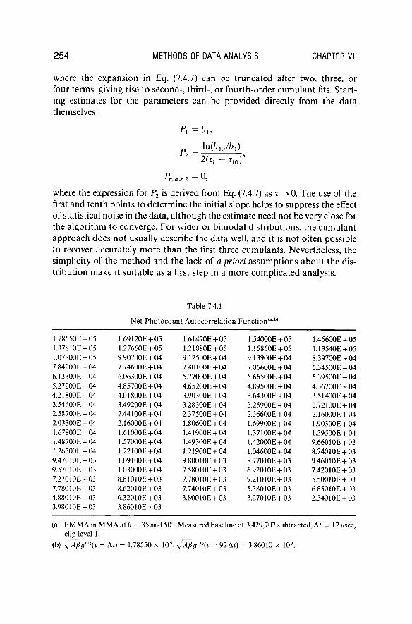
Table 7.4.1

Net Pho tocount Autocorrelat ion Funct ion

1

1.78550E + 05 1.37810E + 05 1.07800E + 05 7.84200E + 04 6.13300E + 04 5.27200E + 04 4.21800E + 04 3.54600E + 04 2.58700E + 04 2.03300E + 04 1.67800E + 04 1.48700E + 04 1.26300E + 04 9.47010E + 03 9.57010E + 03 7.27010E + 03 7.78010E + 03 4.88010E + 03 3.98010E + 03

1.69120E + 05 1.27660E + 05 9.90700E + 04 7.74600E + 04 6.06300E + 04 4.85700E + 04 4.01800E + 04 3.49200E + 04 2.44100E + 04 2.16000E + 04 1.61000E + 04 1.57000E + 04 1.22100E + 04 1.09100E + 04 1.03000E + 04 8.81010E + 03 8.62010E + 03 6.32010E + 03 3.86010E + 03

1.61470E + 05 1.21880E + 05 9.12500E + 04 7.40100E + 04 5.77000E + 04 4.65200E + 04 3.90300E + 04 3.28300E + 04 2.37500E + 04 1.80600E + 04 1.41900E + 04 1.49300E + 04 1.21900E + 04 9.80010E + 03 7.58010E + 03 7.78010E + 03 7.74010E + 03 3.80010E + 03



(a) Ρ Μ Μ Α in M M A at θ = 35 and 50°. Measured baseline of 3,429,707 subtracted, Δί = 12 ^sec, clip level 1.

(b) V Ï Ï / Ï0

( 1 )(T = Δί) = 1.78550 χ 1 0

5; y]~Âf}g

(X\x = 92 At) = 3.86010 χ ΙΟ

3.


x2

λ(Ν) 7 = 1 j = 2 7 = 3 7 = 4

1 . 5 9 5 E + 0 9 1 . 0 0 0 E + 0 1 1 . 7 8 6 E + 0 5 2 . 0 9 6 E + 0 3 0 . 0 0 0 E - 0 1 0 . 0 0 0 E - 0 1

1 . 1 2 2 E + 0 9 1 . 0 0 0 E + 0 1 1 . 7 9 2 E + 0 5 2 . 0 8 5 E + 0 3 3 . 1 3 5 E + 0 4 - 5 . 2 4 3 E + 0 7

6 . 9 6 6 E + 0 8 5 . 0 0 0 E + 0 0 1 . 8 0 1 E + 0 5 2 . 0 7 2 E + 0 3 6 . 7 5 8 E + 0 4 - 1 . 1 3 0 E + 0 8

4 . 7 4 3 E + 0 8 2 . 5 0 0 E + 0 0 1 . 8 1 0 E + 0 5 2 . 0 6 4 E + 0 3 9 . 6 7 7 E + 0 4 - 1 . 6 5 2 E + 0 8

4 . 0 5 8 E + 0 8 1 . 2 5 0 E + 0 0 1 . 8 1 9 E + 0 5 2 . 0 6 5 E + 0 3 1 . 1 1 5 E + 0 5 - 2 . 0 2 0 E + 0 8

3 . 7 4 1 E + 0 8 6 . 2 5 0 E - 0 1 1 . 8 2 9 E + 0 5 2 . 0 7 8 E + 0 3 1 . 1 6 6 E + 0 5 - 2 . 3 2 5 E + 0 8

3 . 4 4 8 E + 0 8 3 . 1 2 5 E - 0 1 1 . 8 3 9 E + 0 5 2 . 0 9 9 E + 0 3 1 . 2 3 0 E + 0 5 - 2 . 6 4 3 E + 0 8

3 . 2 2 7 E + 0 8 1 . 5 6 2 E - 0 1 1 . 8 5 0 E + 0 5 2 . 1 2 6 E + 0 3 1 . 4 1 8 E + 0 5 - 2 . 8 6 7 E + 0 8

3 . 0 8 7 E + 0 8 7 . 8 1 2 E - 0 2 1 . 8 6 0 E + 0 5 2 . 1 5 4 E + 0 3 1 . 8 6 8 E + 0 5 - 2 . 7 6 7 E + 0 8

2 . 9 5 1 E + 0 8 3 . 9 0 6 E - 0 2 1 . 8 6 8 E + 0 5 2 . 1 8 6 E + 0 3 2 . 7 3 1 Ε + 0 5 - 2 . 1 8 2 E + 0 8

2 . 7 8 6 E + 0 8 1 . 9 5 3 E - 0 2 1 . 8 7 6 E + 0 5 2 . 2 2 6 E + 0 3 4 . 1 1 1 E + 05 - 1 . 0 9 8 E + 08

2 . 6 3 6 E + 0 8 9 . 7 6 6 E - 0 3 1 . 8 8 5 E + 0 5 2 . 2 7 6 E + 0 3 5 . 8 8 3 E + 0 5 3 . 3 2 0 E + 0 7

2 . 5 5 7 E + 0 8 4 . 8 8 3 E - 0 3 1 . 8 9 4 E + 0 5 2 . 3 2 3 E + 0 3 7 . 5 5 0 E + 0 5 1 . 6 9 1 E + 08

2 . 5 3 6 E + 0 8 2 . 4 4 1 E - 0 3 1 . 8 9 9 E + 0 5 2 . 3 5 2 E + 0 3 8 . 5 7 3 E + 0 5 2 . 5 3 2 E + 0 8

2 . 5 3 4 E + 0 8 1 . 2 2 1 E - 0 3 1 . 9 0 1 E + 0 5 2 . 3 6 2 E + 0 3 8 . 9 4 0 E + 0 5 2 . 8 3 6 E + 0 8

2 . 5 3 4 E + 0 8 6 . 1 0 4 E - 0 4 1 . 9 0 2 E + 0 5 2 . 3 6 4 E + 0 3 9 . 0 1 0 E + 0 5 2 . 8 9 5 E + 0 8

2 . 5 3 4 E + 0 8 3 . 0 5 2 E - 0 4 1 . 9 0 2 E + 0 5 2 . 3 6 4 E + 0 3 9 . 0 1 7 E + 0 5 2 . 9 0 0 E + 0 8

2 . 5 3 4 E + 0 8 1 . 5 2 6 E - 0 4 1 . 9 0 2 E + 0 5 2 . 3 6 4 E + 0 3 9 . 0 1 7 E + 0 5 2 . 9 0 1 E + 0 8

(a) [G<

2 )(T) - Λ ] = Ρ ι βχ ρ [ 2 ( - Ρ2τ + Ρ 3τ

2- -•··)]· Third-order fit to 9 2 points beginning with

first point. (b) Γ = 2 . 3 6 χ 1 0

3s e c -

1; ju 2/ f

2 = 0 . 3 2 3 .

(c) The iterative sequence used for comput ing the P/s was terminated when none of the pa rameters changed by more than 0 . 1 % between successive iterations.

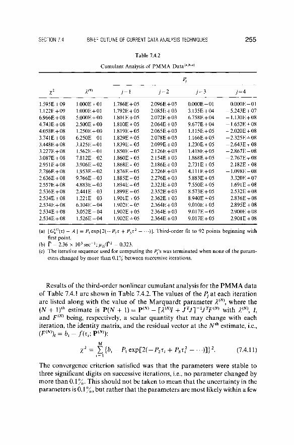
Results of the third-order nonlinear cumulant analysis for the P M M A data of Table 7.4.1 are shown in Table 7.4.2. The values of the Pj at each iteration are listed along with the value of the Marquardt parameter λ

(Ν\ where the

(N + l )th estimate is P(JV + 1) = P

( N) - [A

( iV)7 + J

Tjy

lJTF

m with λ

{Ν\ 7,

and FiN) being, respectively, a scalar quantity that may change with each

iteration, the identity matrix, and the residual vector at the Nth estimate, i.e.,

(F{N))i = bt - /(τ,; P W ) :

M

Χ2=Σ i

bi - Λ β χ ρ [ 2 ( - Ρ 2τ , + Ρ3τ? - • • • ) ]}

2. (7.4.11)

The convergence criterion satisfied was that the parameters were stable to three significant digits on successive iterations, i.e., no parameter changed by more than 0 .1%. This should not be taken to mean that the uncertainty in the parameters is 0.1 %, but rather that the parameters are most likely within a few

Table 7 . 4 . 2

Cumulan t Analysis of P M M A D a t a

( a b c)


tenths of a percent of the values they will eventually converge to. The variance is defined as μ 2/ Γ

2, and a value of 0.323 indicates a reasonably wide dis

tribution for this sample.

7.5. MULTIEXPONENTIAL SINGULAR-VALUE DECOMPOSITION (MSVD)

The MSVD scheme is inferior to C O N T I N , but it is simpler to implement and can be used reasonably successfully for fairly broad unimodal distributions.

In the MSVD approach, G(T) is approximated by a weighted sum of Dirac delta functions:

G(T)= X PjS(r-rj). (7.5.1)

Linear methods fix the location of the ^-function (i.e., the Γ}) and fit for best values of the Py, nonlinear methods allow the Γ} to float as well. The choice of the number of ^-functions n, and hence the number of adjustable parameters (n for the linear approximations, In for the nonlinear), depends upon the method of inversion that is to be used. It must be kept in mind that the amount of information available is limited. Unless the method of inversion includes an appropriate rank-reduction step, the range in G(T) determines n, as the resolution is fixed by the noise on the data. The nonlinear methods rapidly become very time-consuming and are subject to convergence problems as η is increased. In practice it is found that the nonlinear model, where the location of the ^-functions is an adjustable parameter, is essentially limited to the determination of a double-exponential decay, i.e., η = 2. The nonlinear problem can be solved by standard nonlinear least-squares techniques. By writing our model as

G(T) = \νδ(Γ- Γ,) + (1 - νν)(3(Γ - Γ2), (7.5.2)

where w is a normalized weighting factor, we have, after appropriate substitution of Eq. (7.5.2) into Eq. (7.1.1),

bt = Λ exp( - P2TT) + P 3 exp( - P^t)9 (7.5.3)

with the elements of the Jacobian given by

j n = - e x p ( - P 2T t) ,

Ji2 = Ρίτίεχρ(-Ρ2τί)9 Ji3 = - e x p ^ T , . ) ,

S E C T I O N 7.5 M U L T I E X P O N E N T I A L S I N G U L A R - V A L U E D E C O M P O S I T I O N ( M S V D ) 2 5 7

Initial estimates of the parameters can be obtained from the results of the cumulant analysis; we have found it simpler and usually sufficient to use the starting values

P, = P3 = bJX

P2 = Γ/2,

P 4 = 2f,

where Γ is estimated from the initial slope of the correlation function as in the cumulant technique.

The linear least-squares minimization problem can be stated as

C P ~ b, (7.5.5)

where C is the (Μ χ η) curvature matrix, Ρ is the parameter vector of length n9 and b is again the data vector of length M. M and η are, respectively, the number of data points in the net correlation function and the number of adjustable parameters of the model. For example, under the linear multiex-ponential approximation, the elements of C can be determined from comparison of Eqs. (7.1.1) and (7.5.1) with Eq. (7.5.5) to be

c v = e~r^ (7.5.6)

where i and j are the row and column indices, respectively, and the parameters to be determined are the Pj9 i.e., the weighting factors of the ^-functions (see Eq. (7.5.1)). The symbol ~ in Eq. (7.5.5) is intended to imply solution of the overdetermined set of equations subject to the least-squares criterion (minimization of the Euclidean norm of the residual vector ||b — CP | | , where the Euclidean norm of a vector h can be computed from | |h| | = (Σ^

2)112

). Prior to entering the singular-value decomposition routine, we generally scale the columns of C to unit norm in order to improve the numerical stability of the inversion (see for example, Lawson and Hanson, 1974, pp. 185-188). The scaling transforms Eq. (7.5.5) to

Ax ~ b, (7.5.7) where

A = CH (7.5.8) and

x = H1F9 (7.5.9)

with H being a diagonal matrix whose nonzero elements are the reciprocals of the norms of the corresponding column of C,

/ η \ - l / 2 (7.5.10)


The resulting problem (Eq. (7.5.7)) is passed to a singular-value decomposition algorithm (for example, subroutine S V D R S from Appendix C of Lawson and Hanson, 1974), which transforms Eq. (7.5.7) to

t / S F "1x = b, (7.5.11)

where U and V1 are orthogonal matrices and S is a diagonal matrix whose

nonzero elements are the (monotonically decreasing) singular values of the stated problem. The explicit procedure of finding this singular-value decomposition (i.e., determining the matrices U, S, and V~

l) involves the applica

tion of properly chosen orthogonal transformations to the matrix A such that Eq. (7.5.11) holds; details of the procedure may be found in Lawson and Hanson (1974) and will not be discussed further. It is precisely this decomposition that subroutine S V D R S of Lawson ancd Hanson's book accomplishes. Defining the new vectors y and g by

χ = Vy (7.5.12)

and

g = UTb, (7.5.13)

we have

Sy = g . (7.5.14)

The singular-value routine will typically return the matrices V and S and the vector U

Tb. Since S is diagonal, we have immediately

* = (7-5.15)

with Si being the ith singular value, Stj. Equation (7.5.15) represents the full-rank solution to the problem (7.5.7) and

assumes that all singular values are nonzero, i.e., the problem was nonsingular. This is generally not the case, since Eq. (7.5.7) is often pseudorank-deficient in that not all η elements of χ are recoverable as independent resolution elements, due to the data noise. A rank-reduction step is employed to limit the amount of information necessary to express the solution. If we know the problem to be of pseudorank k, we can retain the first k diagonal elements of S and ignore the rest, i.e., we compute the pseudoinverse of 5, S

+, and place zeros in the

locations of S+ that correspond to near-zero singular values st. This is con

sistent with the viewpoint of information theory, since the squares of the singular values are the eigenvalues of the matrix A*A (A* is the adjoint of A) and thus are closely related to the fundamental elements of resolution transmitted through the integral operator of Eq. (7.1.1). Generally, k is unknown; we therefore define a set of "candidate solutions" x

( k) from

S E C T I O N 7.5 M U L T I E X P O N E N T I A L S I N G U L A R - V A L U E D E C O M P O S I T I O N ( M S V D ) 2 5 9

Eq. (7.5.12) as

Vy(k), (7.5.16)

where

O

for 1 < i < fc, for k < i < n.

(7.5.17)

In terms of the original problem (Eq. (7.5.5)) we have a set of candidate solutions for the vector Ρ defined by

Furthermore, this procedure defines a set of residual vectors r(k) such that

There are several criteria for the selection of the particular value of k that can be applied (see Chapters 25 and 26 of Lawson and Hanson, 1974). One that we have found useful is to examine a plot of ln| |r

( f c )| | vs ln | |P

( f c )| | . We

endeavor to select k such that | |r( / c )

| | is sufficiently small without | |P( f c )

| | getting too large. This is directly analogous to the "energy" constraint of some regularization methods. | |h| | denotes the L

2 norm of h(x) on [ x ! , x 2] with

Subroutine S V D R S of Lawson and Hanson would seem to deal satisfactorily with possible numerical problems that might arise during computation. Alternatively the IMSL routine L S V D F or equivalent may be used; again we caution the amateur computer enthusiast against attempting to improve on these routines.

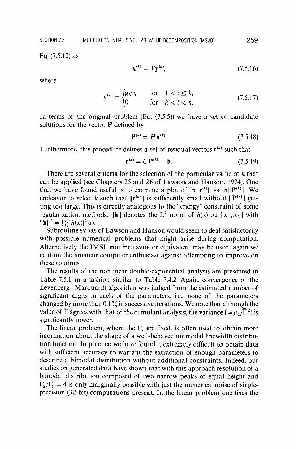
The results of the nonlinear double-exponential analysis are presented in Table 7.5.1 in a fashion similar to Table 7.4.2. Again, convergence of the Levenberg-Marquard t algorithm was judged from the estimated number of significant digits in each of the parameters, i.e., none of the parameters changed by more than 0.1% in successive iterations. We note that although the value of Γ agrees with that of the cumulant analysis, the variance ( = μ 2/ Γ

2) is

significantly lower. The linear problem, where the Γ, are fixed, is often used to obtain more

information about the shape of a well-behaved unimodal linewidth distribution function. In practice we have found it extremely difficult to obtain data with sufficient accuracy to warrant the extraction of enough parameters to describe a bimodal distribution without additional constraints. Indeed, our studies on generated data have shown that with this approach resolution of a bimodal distribution composed of two narrow peaks of equal height and Γ2/Γχ = 4 is only marginally possible with just the numerical noise of single-precision (32-bit) computations present. In the linear problem one fixes the

p(fc) = H xw (7.5.18)

r( k ) = Cp ( k ) _ 5 (7.5.19)

\\h\\2 = i

x

x]\h(x)\2dx.


I

2 j = 1 ) = 2 3 = 3 i = 4

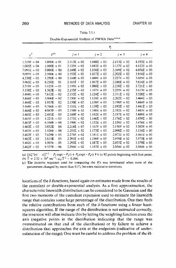
1.519E + 04 1.000E + 01 2. 113E + 02 1.048E + 03 2.113E + 02 4.192E + 03 1.085E + 04 1.000E + 01 2. 125E + 02 1.042E + 03 2.137E + 02 4.122E + 03 7.09 IE + 03 5.000E + 00 2. 140E + 02 1.036E + 03 2.169E + 02 4.036E + 03 5.097E + 03 2.500E + 00 2. 153E + 02 1.037E + 03 2.202E + 02 3.954E + 03 4.339E + 03 1.250E + 00 2. 160E + 02 1.048E + 03 2.227E 02 3.885E + 03 3.965E + 03 6.250E - 01 2. 161E + 02 1.067E + 03 2.240E + 02 3.814E + 03 3.719E + 03 3.125E - 01 2. 159E + 02 1.088E + 03 2.238E + 02 3.721E + 03 3.558E + 03 1.562E - 01 2. 155E + 02 1.107E + 03 2.225E + 02 3.613E + 03 3.484E + 03 7.812E - 02 2. 152E + 02 1.124E + 03 2.211E + 02 3.520E + 03 3.466E + 03 3.906E - 02 2. 150E + 02 1.134E + 03 2.202E + 02 3.464E + 03 3.464E + 03 1.953E - 02 2. 150E + 02 1.138E + 03 2.198E + 02 3.444E + 03 3.464E + 03 9.766E - 03 2. 151E + 02 1.139E + 03 2.195E + 02 3.441E + 03 3.464E + 03 4.883E - 03 2. .154E + 02 1.140E + 03 2.192E + 02 3.443E + 03 3.463E + 03 2.44IE - 03 2. 160E + 02 1.142E + 03 2.187E + 02 3.449E + 03 3.463E + 03 1.221E - 03 2. .171E + 02 1.146E + 03 2.176E + 02 3.459E + 03 3.463E + 03 6.104E - 04 2. 190E + 02 1.152E + 03 2.158E + 02 3.476E + 03 3.463E + 03 3.052E - 04 2. 218E + 02 1.162E + 03 2.130E 02 3.502E + 03 3.463E + 03 1.526E - 04 2. 251E + 02 1.173E + 03 2.098E + 02 3.534E + 03 3.462E + 03 7.629E - 05 2, ,278E + 02 1.181E + 03 2.072E + 02 3.561E + 03 3.462E + 03 3.815E - 05 2. 29 IE + 02 1.186E + 03 2.059E + 02 3.575E + 03 3.462E + 03 1.907E - 05 2. 295E + 02 1.187E + 03 2.055E + 02 3.579E + 03 3.462E + 03 9.537E - 06 2. 296E + 02 1.187E + 03 2.054E + 02 3.580E + 03

(a) [G[

2){T) - ΑΫ

12 = ΡΊ e x p ( - P 2i ) + P 3 exp( - Ρ4τ). Fit to 92 points beginning with first point.

(b) Γ - 2.32 χ 10

3 s e c

- 1; μ2/Τ

2 = 0.266.

(c) The iterative sequence used for comput ing the P/s was terminated when none of the parameters changed by more than 0 .1% between successive iterations.

locations of the (5-functions, based again on estimates made from the results of the cumulant or double-exponential analysis. As a first approximation, the characteristic linewidth distribution can be considered to be Gaussian and the first two moments of the cumulant expansion used to estimate the linewidth range that contains some large percentage of the distribution. One then finds the relative contributions from each of the (5-functions using a linear least-squares algorithm. If the range of the distribution is not estimated correctly, the inversion will often indicate this by letting the weighting function cross the axis (negative points in the distribution indicating that the range was overestimated on that end of the distribution) or by failure to achieve a distribution that approaches the axis at the endpoints (indicative of underestimation of the range). One must be careful to address the problem of the ill-

Table 7.5.1

Double-Exponent ia l Analysis of P M M A D a t a

( a b c)

S E C T I O N 7.5 M U L T I E X P O N E N T I A L S I N G U L A R - V A L U E D E C O M P O S I T I O N ( M S V D ) 261

conditioning properly, however, as the trends described above can be a result of overspecification of the problem rather than true indicators of the proper linewidth range.

The multiexponential problem with fixed ^-functions can be further modified by the introduction of a priori constraints such as nonnegativity, smoothness, etc. In these cases, the problem again becomes a nonlinear one, and the choice of minimization must be made carefully and with a full understanding of the problem of the ill-posedness, since the aim of the introduction of the constraints is to reduce the ill-conditioning, and one must be cognizant of how much improvement has been effected.

Substituting the model (7.5.1) into Eq. (7.1.1) gives

bt= Σ Ρ , β χ ρ ί - Γ , τ , ) . (7.5.20)

In this linear problem, the elements of C are as described in Eq. (7.5.6) above, and the vector Ρ holds the weighting factors Pj.

It should be added here that the eigenvalue analysis of the Laplace transform by McWhirter and Pike (1978) showed that the Γ, should be spaced logarithmically in Γ (i.e., linear spacing in In Γ) to maximize the transmission of information across Eq. (7.1.1). When the ^-functions are spaced unequally, e.g., logarithmically, one should be careful in viewing the results. We have implicitly assumed that the continuous distribution can be sufficiently well represented by the discrete model. It must be kept in mind that the model, and thus the results, are discrete. One cannot draw a line between the points (Γ}, Pj) and expect it to be a picture of the continuous distribution. If it is desired to estimate the behavior of the (assumed to be approximately equivalent) continuous distribution, one must correct for the unequal spacing of the Γ,. This can be done by plotting the points (Γ,-,^/Γ,·) and drawing a continuous curve through them, as has been shown in the figures that show the multi-exponential analysis results (Fig. 7.5.1(a)-(d)), with dashed vertical lines drawn from the Γ-axis to the curve to represent the locations of the functions used in the model. It is imperative to keep in mind that although the output of the algorithm can be a large number of parameters (typically 20), this does not mean that 20 independent parameters have been recovered from the data. Indeed, the vector Ρ is reconstructed from a limited number (fc, typically 3 or 4) of basis functions.

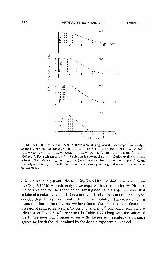
Results of the singular-value decomposition analysis of the multiexponential approximation applied to the P M M A data are shown in Fig. 7.5.1(a)-(d). Initial estimates were obtained from the cumulant results and a little Kentucky windage. In Fig. 7.5.1(a) is shown the k = 3 solution to the problem where the range of G(T) was overestimated. The zeros of G(T) were interpolated and used as improved estimates of the range; this process was repeated


( • )

- l L -ρ

ο

Γ X ID ? S G C

FIG. 7.5.1. Results of the linear multiexponential singular-value decomposit ion analysis of the PMMA da ta of Table 7.4.1. (a) r m in = 50 s e c "

1, r m ax - 10

4 s e c "

1; (b) r m in = 100 s e c

- 1,

rm ax = 8000 s e c "

1; (c) r m in = 135 s e c "

1, T m ax = 7000 s e c "

1; (d) T m in = 260 s e c "

1, Ymax =

5700 s e c "

1. For each range the k = 3 solution is shown; the k = 4 solution exhibited similar

behavior. The values of r m in and r m ax in (b) were estimated from the axis intercepts of (a), and similarly (c) from (b). (d) was the first solution satisfying positivity, and occurred several iterations after (c).

(Fig. 7.5.1(b) and (c)) until the resulting linewidth distribution was nonnega-tive (Fig. 7.5.1(d)). At each analysis, we required that the solution we felt to be the correct one for the range being investigated have a k + 1 solution that exhibited similar behavior. If the k and k + 1 solutions were not similar, we decided that the results did not indicate a true solution. This requirement is overstrict, but is the only one we have found that enables us to detect the occasional misleading results. Values of Γ and μ 2/ Γ

2 computed from the dis

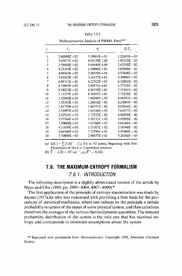
tribution of Fig. 7.5.1(d) are shown in Table 7.5.2 along with the values of the Pj. We note that Γ again agrees with the previous results; the variance agrees well with that determined by the double-exponential method.

S E C T I O N 7 .6 T H E M A X I M U M - E N T R O P Y F O R M A L I S M 2 6 3

Multiexponential Analysis of P M M A D a t a

( aJ

j Γ; PJ Wi

1 2.60000E + 02 3 . 1 9 0 0 1 E - 0 1 1.22693E - 0 3 2 3.05877E + 02 4.45129E + 00 1.45525E - 0 2 3 3.59849E + 02 9.44640E + 00 2.62510E - 0 2 4 4.23345E + 02 1.54904E + 01 3.65906E - 0 2 5 4.98045E + 02 2.28029E + 01 4.57848E-- 0 2 6 5.85925E + 02 3.16337E + 01 5.39894E - 0 2 7 6.89312E + 02 4.22522E + 01 6.12961E - 0 2 8 8.10942E + 02 5.49178E + 01 6.77210E - 0 2 9 9.54033E + 02 6.98258E + 01 7.31901E - 0 2

10 1.12237E + 03 8.70107E + 01 7.75239E-- 0 2 11 1.32042E + 03 1.06200E + 02 8.04292E - 0 2 12 1.55341E + 03 1.26616E + 02 8.15085E - 0 2 13 1.82750E + 03 1.46751E + 02 8.03014E - 0 2 14 2.14997E + 03 1.64188E + 02 7.63677E - 0 2 15 2.52933E + 03 1.75555E + 02 6.94078E - 0 2 16 2.97564E + 03 1.76722E + 02 5.93895E - 0 2 17 3.50069E + 03 1.63260E + 02 4.66364E - 0 2 18 4.11839E + 03 1.31107E + 02 3.18346E - 0 2 19 4.84508E + 03 7.72596E + 01 1.59460E - 0 2 20 5.70000E + 03 2.98877E + 01 5.24346E - 0 5

(a) G{T) = £/5<5(Γ - Γ,·). Fit to 92 points beginning with first. Parameters of the k = 3 candidate solution.

(b) f = 2.30 χ 1 0

3s e c

_ 1; / i 2/ r

2 = 0.262.

7.6. THE MAXIMUM-ENTROPY FORMALISM 7.6.1. INTRODUCTION

The following description is a slightly abbreviated version of the article by Nyeo and Chu (1989, pp. 3999-4004, 4007-4009).*

The first application of the principle of entropy maximization was made by Jaynes (1957a,b), who was concerned with providing a firm basis for the procedures of statistical mechanics, where one induces by the principle a certain probability structure of the states of some physical system, and then calculates therefrom the averages of the various thermodynamic quantities. The induced probability distribution of the system is the only one that has maximal entropy and corresponds to minimum assumptions about the system.

** Reprinted with permission from Macromolecules. Copyright 1989, American Chemical Society.

Table 7.5.2

264 METHODS OF DATA ANALYSIS CHAPTER VII

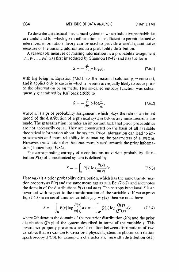
To describe a statistical-mechanical system in which inductive probabilities are useful and for which given information is insufficient to permit deductive inferences, information theory can be used to provide a useful quantitative measure of the missing information in a probability distribution.

A reasonable measure of missing information in a probability assignment ( Ρ Ι , Ρ 2, · · Ί Ρ Ν )

w as fi

fst introduced by Shannon (1948) and has the form

S = - £ A-logPi, (7.6.1)

with log being In. Equation (7.6.1) has the maximal solution pt = constant, and it applies only to cases in which all events are equally likely to occur prior to the observation being made. This so-called entropy function was subsequently generalized by Kullback (1959) to

S = - t P i ^ i - 9 (7.6.2) i=l Qi

where gt is a prior probability assignment, which plays the role of an initial model of the distribution of a physical system before any measurements are made. The generalization includes an important fact: that prior probabilities are not necessarily equal. They are constructed on the basis of all available theoretical information about the system. Prior information can lead to improvements and more reliability in estimating the parameters of a system. However, the solution then becomes more biased towards the prior information (Toutenburg, 1982).

The corresponding entropy of a continuous univariate probability distribution P(x) of a mechanical system is defined by

S = - P(x)log^ldx. (7.6.3) J Ω Mx)

Here m(x) is a prior probability distribution, which has the same transformation property as P(x) and the same meanings as gt in Eq. (7.6.2), and Ω denotes the domain of the distributions P(x) and m(x). The entropy functional S is an invariant with respect to the transformation of the variable x. If we express Eq. (7.6.3) in terms of another variable y, y = y(x), then we must have

S = - f P(x)\og^\dx = - f Q(y)\og^-dy, (7.6.4)

where Ω* denotes the domain of the posterior distribution Q(y) and the prior distribution Q°(y) of the system described in terms of the variable y. This invariance property provides a useful relation between distributions of two variables that we can use to describe a physical system. In photon correlation spectroscopy (PCS), for example, a characteristic linewidth distribution G(T)


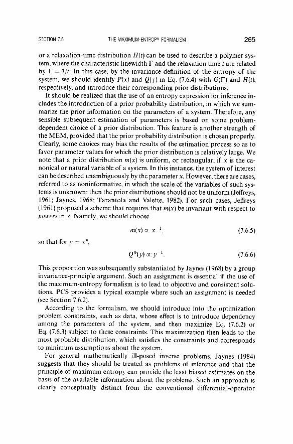
or a relaxation-time distribution H(t) can be used to describe a polymer system, where the characteristic linewidth Γ and the relaxation time t are related by Γ = 1/t. In this case, by the invariance definition of the entropy of the system, we should identify P(x) and Q(y) in Eq. (7.6.4) with G(T) and H(t\ respectively, and introduce their corresponding prior distributions.

It should be realized that the use of an entropy expression for inference includes the introduction of a prior probability distribution, in which we summarize the prior information on the parameters of a system. Therefore, any sensible subsequent estimation of parameters is based on some problem-dependent choice of a prior distribution. This feature is another strength of the M E M , provided that the prior probability distribution is chosen properly. Clearly, some choices may bias the results of the estimation process so as to favor parameter values for which the prior distribution is relatively large. We note that a prior distribution m(x) is uniform, or rectangular, if χ is the canonical or natural variable of a system. In this instance, the system of interest can be described unambiguously by the parameter x. However, there are cases, referred to as noninformative, in which the scale of the variables of such systems is unknown; then the prior distributions should not be uniform (Jeffreys, 1961; Jaynes, 1968; Tarantola and Valette, 1982). For such cases, Jeffreys (1961) proposed a scheme that requires that m(x) be invariant with respect to powers in x. Namely, we should choose

m ( x ) o c x_ 1

, (7.6.5)

so that for y = χ",

Q°{y)Ky-K (7.6.6)

This proposition was subsequently substantiated by Jaynes (1968) by a group invariance-principle argument. Such an assignment is essential if the use of the maximum-entropy formalism is to lead to objective and consistent solutions. PCS provides a typical example where such an assignment is needed (see Section 7.6.2).

According to the formalism, we should introduce into the optimization problem constraints, such as data, whose effect is to introduce dependency among the parameters of the system, and then maximize Eq. (7.6.2) or Eq. (7.6.3) subject to these constraints. This maximization then leads to the most probable distribution, which satisfies the constraints and corresponds to minimum assumptions about the system.

For general mathematically ill-posed inverse problems, Jaynes (1984) suggests that they should be treated as problems of inference and that the principle of maximum entropy can provide the least biased estimates on the basis of the available information about the problems. Such an approach is clearly conceptually distinct from the conventional differential-operator


regularization approach. The major difference is that in the maximum-entropy (regularization) formalism, correlations in the maximal-entropy solution are dictated purely by data and by the nature of a problem, while in the differential-operator formalism, correlations are also effected by our choice of the order of an operator. In the next subsection, we shall describe how the maximum-entropy formalism can be applied to analyzing PCS data.

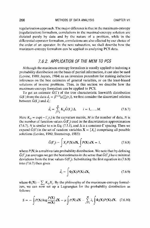
7.6.2. APPLICATION OF THE MEM TO PCS Although the maximum-entropy formalism is usually applied to inducing a

probability distribution on the basis of partial information, it can also be used (Levine, 1980; Jaynes, 1984) as an inversion procedure for making inductive inferences on the best estimates of general variables, or on the least-biased solutions of inverse problems. Thus, in this section we describe how the maximum-entropy formalism can be applied to PCS.

To get an estimate G(T) of the true characteristic linewidth distribution G(T) from the data dt = β

1 1 2^ ^ ^ , we first consider the discretized relation

between G{T}) and d{.

1= £κ0.Ο(Γ,.)Δ, i = l , . . . , M . (7.6.7)

Here Ktj = exp( — Γ,-τ,) is the curvature matrix, M is the number of data, Ν is the number of function values G(Tj) used in the discretization approximation (7.6.7), Ν is similar to η in Eq. (7.5.1), and Δ is a constant-Γ spacing. Then we expand G(V) in the set of random variables X = {Xj} comprising all possible solutions (Levine, 1980; Steenstrup, 1985):

G{Tj) = XjP(X) dX, jV(X) dX = 1, (7.6.8)

where P(X) is a multivariate probability distribution. We note that by defining G(Tj) as averages we get the best estimates in the sense that G(I~}) have minimal deviations from the true values G(I~}). Substituting the first equation in (7.6.8) into (7.6.7) then gives

Γφί(Χ)Ρ(Χ)άΧ9 (7.6.9)

where Ot(X) = Σ7·^ο'^0· By the philosophy of the maximum-entropy formalism, we can now set up a Lagrangian for the probability distribution as follows:

S = P(X)\og^dX - μjp(X)dX - Σ λι|φ,(Χ)Ρ(Χ)«: (7.6.10)


Here, as usual, m(X) is a prior distribution, and μ and k{ are Lagrange multipliers, whose values are fixed by the conditions (7.6.8). Maximizing (7.6.10) with respect to P(X) then leads to the Eule r -Lagrange equation (Jaynes, 1957; Jaynes, 1957; Levine and Tribus, 1979; Levine, 1980)

P(X) = m(X)exp - 1 - μ - Σ W X )

or the partition function

^ = Σλίκυ = exp(l + μ) = m(X) exp

(7.6.11)

dX. (7.6.12)

Equation (7.6.12) is in fact a general expression for an inverse problem. For an inverse problem, we only have to define a prior distribution m(X) and a kernel Ky. By using Eq. (7.6.12), we can calculate G(Tj) and d, by Eq. (7.6.8) and (7.6.9), respectively. But we should remember to relate the experimental data dt with the data estimates dt by some statistic criterion, such as a χ

2 constraint. The χ

2

condition that we shall use is characterized by

Z2 =

d,- - d. = Σ

d; - d; = M, (7.6.13)

which simply indicates that the estimated or predicted and the observed spreads in the observations are, on the average, equal for each channel value.

Equally important is to provide an estimate of the error-squared deviations of of the data dt. A data analysis method without some sort of error estimate is useless. Since a general analytic expression for of, which includes all possible experimental conditions, is not accessible, an approximation is necessary. We shall assume that the squared deviations of the correlation have a Poisson profile, so that the deviations of dt are given by (Bartlett, 1947; Kendall and Stuart, 1968)

_2 1 + ^2

4Ad2

(7.6.14)

Equation (7.6.14) exhibits a reasonable feature of a correlation function: that data at longer delay times have larger of. The form of of can be pivotal in the effective use of the M E M approach. This is a point often overlooked by investigators who want to improve the resolving power of the M E M . (See Appendix 7.B.)

With some prescribed m(X), the Laplace inversion problem now consists of solving Eqs. (7.6.9), (7.6.12), and (7.6.13) for the parameters {^} or { a j . This problem in its present form is numerically inefficient (Alhassid et al., 1978). So instead of solving these equations, we shall use an equivalent but simpler maximum-entropy formalism (Levine, 1980; Steenstrup, 1985). Since a characteristic linewidth distribution is semipositive and bounded, we can take it


as a probability density. Thus, we can define

" Ό: £(Γ;·)Δ

M Mj L

G(

rj )

A

j

as the entropy of our system, where pj is the representative fraction of particles (or macromolecules) with characteristic linewidth in the interval (Γ,· — Δ/2, Tj + Δ/2). Here Δ is a constant spacing and Γ, are equally spaced. However, in this case, the prior model distribution {m,-} is not uniform. As mentioned in Section 7.6.1, the scale of the parameter Γ is α priori unknown. So we should choose m3 oc 1/Γ,·, which is an objective choice. We can take either a characteristic linewidth Γ or a relaxation (or decay) time t (= 1/Γ) as a parameter for describing a system. The objective choice for the prior distribution is then either m, oc 1/Γ, or m J oc 1/tj (cf. Eqs. (7.6.5) and (7.6.6)). Otherwise, the choice of m, = constant would lead to m° oc 1/(ί,·)

2 and not to

ra° = constant, and vice versa. If we now describe the problem in terms of In Γ or In t, we can use objectively a uniform prior distribution. This choice also makes the description of a characteristic linewidth distribution more effective, so that very wide distributions can be better specified. Accordingly, we should define the fractions of particle sizes in the interval (In Γ} — Δ/2, In Γ} + Δ/2) as Fj = GCT^Tj Δ, where Δ = (In — In I"i)/(N — 1) is a spacing in In Γ, and Ν is the number of logarithmically spaced values satisfying In Tj+1 = In Γ} + Δ. Normally, to describe very broad and multimodal distributions, we may take any value of Ν between 30 and 100. (In our program Ν = 81 is used.) The lower and upper bounds Tx and FN are chosen such that G(I"i) and G(FN) are negligibly small. It should be emphasized that in order to define G(T), sample times should be chosen such that the relations ΓΝ = 1/τ1 and Γχ = 0.01/τΜ are approximately satisfied (Provencher, 1979), where τι and τΜ are the delay times of the first and the last channel, respectively. We can now use Fj as our "probabilities" and a uniform prior distribution to define an entropy expression. In this case the Laplace transform simply reads

1 = Σ FjKv> K

i j = e x p i - I » , (7.6.16)

where Ktj is the curvature matrix (kernel). We should note that since in PCS characteristic linewidth distributions are only normalized to V/?, i.e., Σ j Fj — Vj8, the probabilities should be p. = FJ/^JFJ. But the entropy depends only on the form of {Fj} and not on its normalization; thus it is computationally advantageous to use the following definition:


where b and A0 ( = b/e, e = 2.718...) are constants with A0 being a default or predetermined value (Burch et al, 1983; Gull and Skilling, 1984), which in the absence of data constraint is the maximal solution of Eq. (7.6.17). Here we choose A0 = \[β/Ν, so that Fj and A0 are normalized to y/β. The inverse problem now amounts to maximizing Eq. (7.6.17) subject to the χ

2 constraint

(7.6.13) and the transform (7.6.16).

7.6.3. THE MAXIMAL-ENTROPY SOLUTION In this section, we shall briefly describe a quadratic model approximation

for solving the nonlinear maximum-entropy problem and how the solution can be attained.

The problem can be stated as follows: maximize the objective function with respect to the distribution {Fj},

S — j ^ l n ^ - F , ) (7 .6 ,7)

subject to the χ2 constraint

M {2- - d\2

X2=l[\^) =Af, (7.6.13)

where df = Vj5|gf(1)

(Ti)| are the estimates on the data dt and are related to Fj by Eq. (7.6.16). Equations (7.6.13), (7.6.16), and (7.6.17) describe a nonlinearly equality-constrained optimization problem and can be solved by several standard approaches (Wismer and Chattergy, 1978; Harley, 1986; Freeman, 1986; Beightler et al, 1979). For instructional purposes, we briefly describe a quadratic model approximation method described by Burch et al (1983) (see also Skilling and Bryan, 1984; Skilling and Gull, 1985).

The quadratic model approximation approach amounts to first approximating Eqs. (7.6.13) and (7.6.17) as

N rJS 1

N f)

2S

S = S0+ Σ 6Fj + -Y j-—èFjôFk, (7.6.18 ) MdFj 2j%dFjdF k N

dv2 1

N d

2v2

Ϊ ' ' ά + Σ ^ , + -2ΐφ^, (7-6.!9)

where ôFj are the corrections to F ° = A0 (the default value), at which S0, χΐ, and the derivatives of S and χ

2 are evaluated. Note that the χ

2 expansion

terminates at the second derivative and is therefore exact. However, since the entropy function is highly nonlinear, the quadratic expansion of it is only approximately valid locally about F ° = A; that is, the quadratic term in


Eqs. (7.6.18) must be smaller than its preceding terms. It is necessary to set an upper bound on the quadratic term:

- g ^ W S O j C F j , (7.6.20)

which is chosen by practical experience. For nonlinear models, it is necessary to solve for the solution iteratively by

calculating the corrections SFj to the preceding approximate distribution. Thus, in the first iteration we calculate

Fj = f ° + SFj (7.6.21)

and use them as the second estimates at which a new quadratic model approximation can be constructed. Then we define SFj in terms of several search directions (normally three is sufficient) in which we make the expansion:

SFj = Σ (7·6·2 2

)

To achieve efficiently the maximization of S under the χ 2 (7.6.13), the following

simple unit vectors are used (Burch et al, 1983):

Fdv2

e ) * ^ - , (7.6.23)

β^41^""2^)· (7A24)

( 7·

6·

2 5) where ax and a 2 are given by

Oil = -1/2 -1/2

(7.6.26)

so that the first and second quantities in Eq. (7.6.24) are normalized with respect to the metric tensor gjk = ôjk/Fj (ôjk being the Kronecker delta). The metric tensor gjk9 which is minus the second derivative of the entropy function, — ô

2S/dFjdFk, provides a local measure of the magnitude and direction

of the corrections (cf. Eq. (7.6.20)) about some map {Fj}. Thus, it is effective to use this metric tensor for defining local quantities. For instance, the unit vectors (7.6.23)-(7.6.25) are normalized according to

Hell2 = twM = !> A* = 1,2,3. (7.6.27) j.k

S E C T I O N 7.6 T H E M A X I M U M - E N T R O P Y F O R M A L I S M 2 7 1

Substituting the three vectors into Eqs. (7.6.18) and (7.6.19), we can rewrite them in terms of χμ(μ = 1 , 2 , 3 ) , respectively, as

μ — 1 μ, ν

Χ2 = ή + Σ Ο μχ μ+

1- Σ ί μ νχ μχ ν, (7.6.29)

μ — 1 ^ μ, ν

where Ν dS

Ν d

2S

UdFjdFk

The distance constraint (7.6.20) reduces simply to

/ = Σ ν * , Λ < 0 . ΐ | > ? . (7.6.32) μ,ν j

A Lagrangian can now be set up: L(x) = ocS — χ2 — /?/, with α and β being

positive parameters. (We note that we can use instead the Lagrangian L\x) = S — α'χ

2 — β'Ι, with positive parameters a' and β\ which amounts

simply to the rescalings L(x) -> aL'(x), α' = l/α, β' = β/α. Thus, here the use of L(x) is purely for convenience.) Maximizing L(x) leads to a set of coupled equations for χμ. For computational efficiency, we first decouple the components χμ by transforming them (Beightler et a/., 1979; Birkhoff and MacLane, 1965) to an orthogonal set {γμ}, so that the matrices or tensors / ιμν and ίμν become diagonal. By so doing, the Lagrangian now reads

3

L(y) = o c S 0- x

2

0+ Σ ( ° 4 - Φ)>μ

μ = 1 (7.6.33)

1 3

V '

- - Χ ( ( α + 2 ^ ) ^ μν + Λ μ μ) ) ^ ν,

where tildes denote quantities that are orthogonally transformed, δμν is a Kronecker delta, and Α μ μ( μ = 1,2,3) are the diagonal elements of the dia-gonalized matrix of ίμ ν. Maximization of this Lagrangian can be carried out in many ways. For example, the fact that Eq. (7.6.33) is stationary with respect to the variations of γμ leads to the Eule r -Lagrange equations for γμ,

γμ = (α5μ - £μ)(α + 2β + AJ'K (7.6.34)


Equation (7.6.34) gives infinitely many maximal-entropy solutions, which are classified by the parameters α and β. Of all the possible solutions we want to find one that satisfies our statistical criterion and the distance constraint (7.6.32), which is now given by / = Σμγ^μ· But since at each iteration the minimum attainable #

2-value is (cf. Eq. (7.6.33))

*Ln = x l - \ Σ τ5" - (

7·6·3 5

) 1 μ = 1

Αμμ

which can be larger than our required value M, a slightly higher χ2-value is

imposed to provide some flexibility in the iterative procedure:

Û = Û - \ i C

~ - (7.6.36 ) J μ = 1

Αμμ

Thus, the refined χ2-value in the procedure is given by

χ2 = m a x i m u m ^

2, , χ

2 = M). (7.6.37)

How the solution is chosen is briefly described as follows. At each iteration we first set β = 0 and find the largest a-value such that the required χ

2-value

(7.6.37) is attainable. Then the parameter β is increased until the subsequent solution γμ obeys the distance constraint. If the constraint is not satisfied, the X

2-value is increased to χ

2,. The corrections SFj are then obtained by backward

substitution. The required solution {Fj} is the one that satisfies some terminating criteria,

e.g., m a x l ^ - ^ - ^ l <(5t- (7.6.38)

i and

max \Ff + υ

-Ff \ < ôj. (7.6.39 ) j

Alternatively, th e maximal-entrop y solutio n ca n b e selecte d b y usin g th e following criterion :

ï / h w M< 2χ 1 0

"3

· ,7

·6·40)

where and α2 are given in (7.6.26). Equation (7.6.40) is a measure of the degree of entropy maximization, where the tolerance value of 2 x 1 0 "

3 is

determined on practical grounds. We note that a zero tolerance value corresponds to the ideal maximal solution. In addition, the use of quadratic model approximation unavoidably loses the positivity property of the solution in the iterative procedure. Thus, it is necessary to reset any negative values in each iteration to a small but positive number.


For a set of 136 data points, about 6 seconds is needed for an iteration by using a microcomputer with a 12-MHz 80286 math coprocessor and Microsoft F O R T R A N and about 100 iterations are required. By comparison, one second per iteration is needed if an IBM PS/2 model 80 microcomputer is used.

In Section 7.6, we have pedagogically (1) introduced the maximum-entropy formalism, (2) outlined its use in estimating solutions to inverse problems in general and to the Laplace inverse problem in PCS in particular, and (3) described a quadratic model approach for solving the nonlinearly constrained maximum-entropy optimization problem in PCS, and specified how its solution was achieved. The reliability of the formalism has been tested successfully by using several sets of numerically simulated time-correlation-function data corresponding to known characteristic linewidth distributions.

The main thrust of using the maximum-entropy (MEM) formalism lies in its proven objectivity. In this formalism, information in the maximum-entropy solution is dictated purely by the available data, and not by an arbitrarily introduced differential operator such as one may find in the regularization formalism. The maximum-entropy formalism requires introduction of a prior probability distribution in which we can summarize our prior information. For example, any theoretical information about the physical problem of interest can be taken into account here. Such an introduction depends on the nature of the problem. For most problems, the corresponding prior distributions are uniform. In the Laplace inverse problem in PCS, however, the prior distribution is not uniform but oc l /Γ or ocl/ί , depending on whether the characteristic linewidth distribution G(T) or the relaxation-time distribution H(t) is used for describing the system of interest. This choice of prior distribution leads to adopting a log Γ (or log t) description of G(T) (or H(t)) and hence to specifying very broad G(T) (or H(t)) more effectively.

We have described one method for solving the nonlinear maximum-entropy problem, namely the quadratic model approximation (7.6.3). The quadratic model approximation yields an acceptable solution, which is, unfortunately, not positive definite. Better approaches to solving the M E M problem could undoubtedly be devised (e.g., see Section 7.8). It should, however, be emphasized that knowledge of the error deviations of the experimental data can substantially improve the solution for G(r), including the resolution of G(T). This error knowledge on the experimental data depends on subjective evaluation as well as systematic errors, which may be difficult to estimate. Preliminary analysis methods used for estimating or refining error deviations of measured data may introduce unintended bias into our G(r) reconstruction. It remains to be seen what preliminary analysis method can best provide the least biased data deviations. As the analysis must necessarily depend on the physical nature of the experiment, a generalized approach may be difficult to achieve.


In addition to the noise in the measured data, we have alleviated the bandwidth limitation on the experimentally measured time correlation function by insisting on predetermining the value of β and by letting the first-channel value of the correlation function, | #

( 1 )(Δ ί ) |

2, be greater than 0.998 and the

last-channel value, |#( 1 )

( last channel) |2, be less than 0.005.

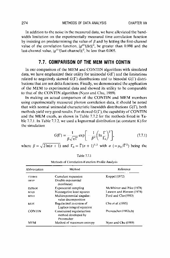
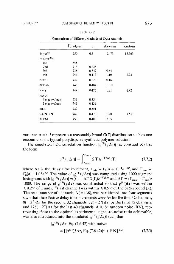
7.7. COMPARISON OF THE MEM WITH CONTIN In our comparison of the M E M and C O N T I N algorithms with simulated

data, we have emphasized their utility for unimodal G(T) and the limitations related to negatively skewed G(T) distributions and to bimodal G(T) distributions that are not delta functions. Finally, we demonstrated the application of the M E M to experimental data and showed its utility to be comparable to that of the C O N T I N algorithm (Nyeo and Chu, 1989).

In making an actual comparison of the C O N T I N and M E M members using experimentally measured photon correlation data, it should be noted that with normal unimodal characteristic linewidth distributions G(T), both methods yield very good results. For skewed G(T), the capability of C O N T I N and the M E M excels, as shown in Table 7.7.2 for the methods listed in Table 7.7.1. In Table 7.7.2, we used a lognormal distribution (at constant K) for the simulation

0 (Γ) = 1

β^/πΓ exp > 0 i (7.7.1)

where β = ^2\η{σ + 1) and Γ0 = Γ(σ + 1 )1 /2

with σ ( = μ 2/ Γ2) being the

Table 7.7.1

Methods of Correla t ion-Funct ion Profile Analysis

Abbreviation Method Reference

CUMFIT Cumulan t expansion Koppel (1972) DEXP Double exponential

(nonlinear) EXPSAM Exponential sampling McWhir ter and Pike (1978) NNLS Nonnegat ive least squares Lawson and Hanson (1974) MSVD Multiexponential singular- Ford and Chu (1983)

value decomposit ion RILIE Regularized inversion of Chu et al (1985)

Laplace integral equat ion C O N T I N Constrained regularization Provencher(1982a,b)

method developed by Provencher

M E M Method of max imum entropy Nyeo and Chu (1989)

S E C T I O N 7 .7 C O M P A R I S O N O F T H E M E M W I T H C O N T I N 2 7 5

Table 7.7.2

Compar ison of Different Methods of D a t a Analysis

Γ, rad/sec σ Skewness Kurtosis

I n p u t

( a) 750 0.5 2.475 15.563

CUMFIT

( B ):

1st 645 2nd 713 0.235 3rd 736 0.349 0.64 4th 744 0.413 1.10 3.73

DEXP 727 0.223 0.167

EXPSAM 743 0.407 1.012

NNLS 749 0.476 1.81 6.92

MSVD:

4 eigenvalues 731 0.354 5 eigenvalues 745 0.436

RILIE 729 0.341

C O N T I N 749 0.476 1.90 7.55

M E M 750 0.488 2.05

variance, σ = 0.5 represents a reasonably broad G(T) distribution such as one encounters in a typical polydisperse synthetic polymer solution.

The simulated field correlation function \g{1)(j Ατ)\ (at constant K) has

the form

ΐ0( 1 )

Ο 'Δτ) | = G(r)e~rjAt

dr9 (7.7.2)

where Δτ is the delay time increment, T m in = Γ0(σ + 1) 1

e 3β

9 and T m ax = Γ0(σ + l)~

1e3p. The value of |^

( 1 )(7"Δτ)| was computed using 1000 segment

histograms with \gw{jAx)\ * £ ( =1 Δ Γ Ο ( ] > - ™

Δ* and ΔΓ = ( r m ax - r m i n) /

1000. The range of g(1)(j Δτ) was constructed so that #

( 1 )(Δτ) was within

^ 0 . 2 % of 1 and #( 1 )

( las t channel) was within ^ 0 . 5 % of the background (A). The total number of channels, N(= 136), was partitioned into four segments such that the effective delay time increments were Δτ for the first 32 channels, 8( = 2

3) Δ τ for the second 32 channels. 32( = 2

5) Δ τ for the third 32 channels,

and 128( = 27) Δ τ for the last 40 channels. A 0 .1% random noise (RN), rep

resenting close to the optimal experimental signal-to-noise ratio achievable, was also introduced into the simulated |^

( 1 )(7*Δτ)| such that

| 0( 1 )

( ; Δ τ , Eq. (7.6.42) with noise)|

= [ | 0( 1 )

( ; Δ τ , Eq. (7.6.42)|2 + R N ]

1 / 2. (7.7.3)


A comparison of two polystyrene species ( M w = 4.48 χ 106 g/mole,

M wM n = 1.14 at 4.7 χ 1 0 "5 g/g, and M w = 2.33 χ 10

5 g/mole, MJMn =

1.06 at 9.5 χ 10~4 g/g) in benzene at 25°C showed comparable findings by

C O N T I N and the M E M (Chu et α/., 1989). Thus, at this time, even with our present algorithm, we can claim the M E M to be at least comparable with C O N T I N . With the improved M E M (Appendix 7.B), the resolution seems to exceed that of C O N T I N . Further improvements (Section 7.8) will continue as we do not yet have a full understanding of the intricate nature of M E M .

7 .8 . M A X I M I M - E N T R O P Y M E T H O D U S I N G A B A Y E S I A N E S T I M A T E F O R T H E

R E G U L A R I Z A T I O N P A R A M E T E R In the introduction to Section 7.4, the reader was reminded that Section 7.6

(on the maximum-entropy formalism) could be skipped by the less mathematically oriented reader. Sections 7.5 and 7.6 were included in this chapter in order to let interested readers see some aspects of the development of one approach to solving the nonlinear maximum-entropy problem. The details for using the M E M approach are complex. For example, by merely changing the form of af from Eq. (7.6.14) to Eq. (7.B.1), we can improve the resolution of M E M as presented in Section 7.6, which, nevertheless, still contains many undesirable features. These could include the problems that the M E M solution in Section 7.6 is very sensitive to baseline fluctuations, and that the G(T) estimates are based on |#

( 1 )(τ) | , which is only indirectly related to the

measured intensity correlation function G( 2 )

( T ) . A new approach to the maximum-entropy analysis has been developed by

using a Bayesian estimate for the regularization parameter. As first suggested by Gull (1989), who showed that the criterion to use χ

2 (Eq. (7.6.13)) tends to

underfit the data, Langowski and Bryan (1990) and Bryan (1990b) reported a new computer program (MEXDLS) specifically designed for dynamic light scattering (DLS) data. With this algorithm (Bryan, 1990a,b), which permitted estimates of the baseline and of the variance of the calculated spectra, a better resolution than C O N T I N could be achieved. Thus, an application of Bayesian statistics to the analysis of intensity time correlation functions seems to be a better approach for retrieving information from multimodal characteristic linewidth distributions. Interested readers should refer to the references for details. It should be noted that there are many volumes of Maximum-Entropy and Bayesian Methods in existence, with the latest two volumes being those edited by Skilling (1989) and by Fougèr e (1990) . Thus , M E M i s on e o f thos e established method s fro m anothe r field. I t i s no t a s eas y a tas k t o transfe r the M E M ove r t o dynami c ligh t scatterin g a s on e migh t expect , especiall y fo r the les s mathematicall y oriente d scientist . Th e reade r shoul d tr y t o obtai n well-tested algorithm s rathe r tha n tryin g t o develo p wha t i s alread y known .

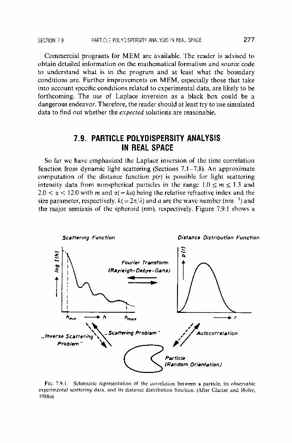
S E C T I O N 7.9 P A R T I C L E P O L Y D I S P E R S I T Y A N A L Y S I S I N R E A L S P A C E 2 7 7

Commercial programs for M E M are available. The reader is advised to obtain detailed information on the mathematical formalism and source code to understand what is in the program and at least what the boundary conditions are. Further improvements on M E M , especially those that take into account specific conditions related to experimental data, are likely to be forthcoming. The use of Laplace inversion as a black box could be a dangerous endeavor. Therefore, the reader should at least try to use simulated data to find out whether the expected solutions are reasonable.

7.9. PARTICLE POLYDISPERSITY ANALYSIS IN REAL SPACE

So far we have emphasized the Laplace inversion of the time correlation function from dynamic light scattering (Sections 7.1-7.8). An approximate computation of the distance function p(r) is possible for light scattering intensity data from nonspherical particles in the range 1.0 < m < 1.3 and 2.0 < α < 12.0 with m and ot( = ka) being the relative refractive index and the size parameter, respectively. k( = 2n/X) and a are the wave number ( n m

- 1) and

the major semiaxis of the spheroid (nm), respectively. Figure 7.9.1 shows a

Scattering Function Distance Distribution Function

FIG . 7.9.1. Schematic representation of the correlation between a particle, its observable experimental scattering data , and its distance distribution function. (After Glat ter and Hofer, 1988a).


schematic representation of the correlation between a particle, its observable experimental data 1(h), and its distance distribution function p(r) with h ( E q E K ) being the scattering vector.

The interpretation of elastic light scattering data in real space for non-spherical and inhomogeneous monodisperse systems (Glatter and Hofer, 1988a) and for the determination of size distributions of polydisperse systems (Glatter and Hofer, 1988b) has been described in some detail.

The inverse scattering problem for p(r) as illustrated in Fig. 7.9.1 has the form 1 00

1(h) hr sin hrdh. (7.9.1) ο

P(r) = 2 In

2

The same truncation problem related to the finite range of h and unavoidable presence of experimental noise are present in the measured time-averaged scattered intensity 1(h). Thus, inversion of 1(h) to get p(r) is an ill-posed problem. Similarly, 1(h) and the size distributions are related by the integrals

1(h) = Dn(R)(j)(h,m,R)dR, (7.9.2)

/(Λ) = | Dm( K ) 0 ( / î , m , K ) ( / ) ( O , m , R ) -1 / 2

^ , (7.9.3)

and

1(h) = I Dx(RW(h,m,R)(l)(<d,m,R)-1 dR

ο

or

1(h) = Di(R)(t>0(h,m,R)dR, (7.9.4)

where Dm(R) and Dn(R) are, respectively, the mass distribution and the number distribution. 0(/i,m,i?) is the scattering function of a particle of size R and relative refractive index m. φ0(Η, R) = φ(Κ m,&)Φ(0, m, R)

1 is the nor

malized 0(/z, m, R). The parameter can be any characteristic dimension of the particle. In the case of spheres, R is the radius. D{(R) ~ R

3Dm(R) ~ R

6Dn(R)

in the Ray le igh -Debye-Gans limit where 2kR(m — 1) « 1, i.e., for small particles with very low relative refractive index. The reader should read the original work (Glatter and Hofer, 1988a,b).

For polydisperse colloids in the presence of interactions, the coupling between scattering power and interactions plays a very important role. Pusey et al. (1982) and Vrij (1982) have considered a hard-sphere mixture based on the Perçus-Yevick approximation. The hard-sphere formalism has been extended to polydisperse colloidal particles of spherosymmetrical arbitrary interaction potential (Licinio and Delaye, 1989).

A P P E N D I X 7.B A N O T H E R P R O P O S E D F O R M FOR σ] 2 7 9

APPENDIX 7.A. (RUF, 1989), RELATION BETWEEN BASELINE UNCERTAINTIES AND df

If we let the measured normalized intensity time correlation function be G

(2)(T)/A, where the accent denotes an estimate of the true value, G

( 2 )( T ) =

G( 2 )

( T , ) + E(xi) with Ε being an error function, and A = ΛΓ8[ίϊ(ί)]2, then

* ^ ( . , + i f ). e ^ _ ^ W é d + £ W i ( 7 A 1) A A AA A

where th e nois e ter m Ε(τ-)/λ is the normalized sum of statistical errors for correlator channel i. More importantly, with AA = A — A and A/A = 1 — (AA/A), the term \_G

2(Ti)/A'](AA/A) represents the deviation of the normal

ized intensity correlation function G(1)(x^lA ( = 1 + df) due to errors in the

baseline AA/A). Thus, a normalization error in the baseline produces a constant shift in G

( 2 )(T f) / i 4 . However, in the Laplace transform, we measure

G( 2 )

( T ; ) , but we need |#( 1 )

(τ ) | such that

A

= G<

2>(T,) G

( 2 )(TT. ) AA | E(TT) {

A A A A

= βϊΟ^Ι2 - ^ ( 1 + W W ) + ! ψ (7.A.2)

A A

. Λ _ ί ί · W » ( . J l ' ) - ¥ + •£ ( ,

',

A J A A

= i i - ^ W ^ +

£ ( T i)

A J A A

Thus, in using di9 the normalization errors AA/A due to baseline uncertainties play a more complex role than merely shifting the first-order electric field correlation function.

APPENDIX 7.B. ANOTHER PROPOSED FORM FOR o - f For a Poisson profile,

1 +df σ} =

4Adf

On closer examination, PCS is seen to be a measure of deviations of Poisson distributions. Thus, statistical fluctuations should be included in the error


deviations. For example, the statistical error can be calculated by considering the signals, which obey a Gaussian distribution. Then af has two features. It is a constant according to the Poisson distribution, but it fluctuates at each data point when compared with the measured data. One proposed form is

which is by no means unique. Its use instead of Eq. (7.6.14) improves the resolution of the M E M . Preliminary simulated tests show that the unproved M E M can resolve two narrow (δ) bimodal distributions with Ti/F2 < 2. Further improvements on the form of af are possible and should be forthcoming.

Alhassid, Y., Agmon, N., and Levine, R. D . (1978). Chem. Phys. Lett. 5 3 , 22. Bartlett, M. S. (1947). Biometrics 3 , 39. Beightler, C. S., Phillips, D. T., and Wilde, D. J. (1979). Foundations of Optimization, 2nd ed.,

Prentice-Hall, Englewood Cliffs, N . J. Bertero, M , Boccaci, P., and Pike, E. R. (1982). Proc. R. Soc. London Ser. A 3 8 3 , 15. Bertero, M., Boccaci, P., and Pike, E. R. (1984). Proc. R. Soc. London Ser. A 3 9 3 , 51. Bertero, M., Brianzi, P., Pike, E. R., de Villiers, G„ Lan, Κ. Η., and Ostrowsky, Ν. (1985). J. Chem.

Phys. 8 2 , 1551. Birkhoff, G. and MacLane, S. (1965). "Survey of Modern Algebra" 3rd ed., MacMil lan, New York. Burch, S. F., Gull, S. F., and Skilling, J. (1983). J. Comp. Vis. Graph. Image Proc. 2 3 , 113. Bryan, R. (1990a). Eur. Biophys. J. 1 8 , 165. Bryan, R. (1990b). In "Maximum-Ent ropy and Bayesian Me thods" (P. F. Fougère , éd.) ,

pp. 221-232 , Dordrecht : Klewe r Academic , Hingham , MA . Chu, Β. (1983). In "The Application of Laser Light Scattering to the Study of Biological Mot ion"

(J. C. Earnshaw and M. W. Steer, eds.), N A T O ASI Vol. A59, pp. 5 3 - 7 6 , Plenum Press, New York and London.

Chu, B., Gulari , E s , and Gulari , Er. (1979). Phys. Scr. 1 9 , 476. Chu, Β , Ford , J. R , and Dhadwal , H. S. (1985). In Methods of Enzymology, Vol. 117 (S. P.

Colowick and N. O. Kaplan, eds.), Chapter 15, pp. 256-297 , Academic Press, New York. Chu, Β., Xu, R , and Nyeo, S.-L. (1989). Part. Part. Syst. Charac. 6 , 34. Dahneke, Β. E , e d , (1983). Essentials of size distribution measurement. In "Measurement of

Suspended Particles by Quasi-elastic Light Scattering," pp. 81 -252 , Wiley, New York. Dhadwal , H. S. (1989). Part. Part. Syst. Charac. 6 , 28. Ford, J. R. and Chu, Β. (1983). In "Proceedings of the 5th Internat ional Conference on Pho ton

Correlation Techniques in Fluid Mechanics" (E. O. Schulz-DuBois, ed.), Springer Ser. Opt . Sc i , p. 303, Springer-Verlag, Berlin and New York.

Fougère, P . F . (ed. ) (1990) . "Maximum-Ent rop y an d Bayesia n Methods , " Da r tmou th , Dordrecht : Klewer Academic , Hingham , MA .

Freeman, T . L . (1986) . In "Numerica l Algori thms " (J . L . M o h a m e d an d J . Walsh , eds.) , Oxfor d University Press , Oxford .

Glatter, O . an d Hofer , M . (1988a) . J. Colloid and Interface Sci. 1 2 2 , 484 . Glatter, O . an d Hofer , M . (1988b) . J. Colloid and Interface Sci. 1 2 2 , 496 .

0.05 (7.B.1)

REFERENCES

R E F E R E N C E S 2 8 1

Golub , G. H. and Reinsch, C. (1970). Numer. Math. 1 4 , 403. Gull, S. F. (1989). In " M a x i m u m Entropy and Bayesian Methods ," (J. Skilling, éd.), pp . 5 3 - 7 1 ,

Dordrecht : Klewer Academic, Hingham, MA. Gull, S. F. and Skilling, J. (1984). IEE Proc. 1 3 1 , 646. Hanson, R. J. (1971). SI AM J. Numer. Anal. 8 , 616. Harley, P. J. (1986). In "Numerical Algori thms" (J. L. Mohamed and J. Walsh, eds.), Oxford

University Press, Oxford. Hobson, A. (1971). "Concepts in Statistical Mechanics," G o r d o n & Breach Science, New York. Isenberg, I , Dyson, R. D., and Hanson, R. (1973). Biophys. J. 1 3 , 1090. Jakeman, E , Pike, E. R., and Swain, S. (1971). J. Phys. A 4 , 517. Jaynes, E. T. (1957a). Phys. Rev. 1 0 6 , 620. Jaynes, E. T. (1957b). Phys. Rev. 1 0 8 , 171. Jaynes, E. T. (1968). IEEE Trans, on Systems Science and Cybernetics SSC -4 , 227. Jaynes, E. T. (1984). In "Inverse Problems" (D. W. McLaughlin, éd.), American Mathemat ical

Society, Providence. Jeffreys, H. (1961). "Theory of Probabili ty," 3rd éd., Oxford University Press, London. Katz, A. (1967). "Principles of Statistical Mechanics: The Information Theory Approach," W. H.

Freeman, San Francisco and London. Kendall, M. G. and Stuart , A. (1968). "The Advanced Theory of Statistics, Vol. 3: Design and

Analysis, and Time-Series," 2nd ed., Hafner, New York. Kojro, Z. (1990). J. Phys. A: Math Gen. 2 3 , 1363. Koppel , D. E. (1972). J. Chem. Phys. 5 7 , 4814. Kullback, S. (1959). "Information Theory and Statistics," Wiley, New York. Landsberg, P. T. (1978). "Thermodynamics and Statistical Mechanics," Oxford University Press,

Oxford. Langowski, J., and Bryan (1990). Prog. Colloid and Polym. Sci. 8 1 , 269. Lawson, C. L. and Hanson, R. J. (1974). "Solving Least Squares Problems," Prentice-Hall,

Englewood Cliffs, N . J. Levine, R. D. (1980). J. Phys. A 1 3 , 91. Levine, R. D and Tribus, M., eds. (1979). "The Max imum Entropy Formalism," conference held at

M I T May 2 - 4 , 1978, M I T Press, Cambridge, Mass. Licinio, P. and Délaye, M. (1989). J. Colloid and Interface Sci. 1 3 2 , 1. Livesey, A. K., Licinio, P , and Délaye, M. (1986). J. Chem. Phys. 8 4 , 5102. McWhirter , J. G. and Pike, E. R. (1978). J. Phys. A; Math. Gen. 1 1 , 1729. Miller, K. (1970). SI AM J. Math. Anal. 1, 52. Nyeo, S.-L. and Chu, Β. (1989). Macromolecules 2 2 , 3998. Oliver, C. J. (1979). J. Phys. A: Math. Gen. 1 2 , 519. Oliver, C. J. (1981). In "Scattering Techniques Applied to Supramolecular and Nonequi l ibr ium

Systems" (S.-H. Chen, B. Chu, and R. Nossal, eds.), N A T O ASI Vol. 373, pp. 121-160, Plenum, New York and London.

Ostrowsky, N., Dornet te , D., Parker , P., and Pike, E. R. (1981). Opt. Acta 2 8 , 1059. Pike, E. R. (1981). In "Scattering Techniques Applied to Supramolecular and Non-equil ibr ium

Systems" (S.-H. Chen, B. Chu and R. Nossal, eds.), p. 179, Plenum, New York. Pike, E. R., Watson, D., and McNeil Watson, F. (1983). In "Measurements of Suspended Particles

by Quasi-elastic light Scattering" (B. E. Dahneke , ed.), Chapter 4, Wiley, New York. Provencher, S. W. (1976a). Biophys. J. 1 6 , 27. Provencher, S. W. (1976b). J. Chem. Phys. 6 4 , 2772. Provencher, S. W., Hendrix, J., DeMaeyer , L., and Paulussen, N . (1978). J. Chem. Phys. 6 9 , 4273. Provencher, S. W. (1979). Makromol. Chem. 1 8 0 , 201. Provencher, S. W. (1982a). Comp. Phys. Comm. 2 7 , 213. Provencher, S. W. (1982b). Comp. Phys. Comm. 2 7 , 229.

2 8 2 M E T H O D S O F D A T A A N A L Y S I S C H A P T E R V I I

Provencher, S. W. (1982c). "CONTIN Users Manua l , " EBL Technical Report DA05, European Molecular Biology Laboratory , Heidelberg.

Provencher, S. W. (1983). In "Proceedings of the 5th Internat ional Conference on P h o t o n Correlation Techniques in Fluid Mechanics" (E. O. Schulz-DuBois, ed.), Springer Ser. Opt . Sc i , p. 322, Springer-Verlag, Berlin and New York.

Pusey, P . N , Fijnaut, Ν. M , and Vrij, A. (1982). J. Chem. Phys. 7 7 , 4270. Ruf, H. (1989). Biophys. J. 5 6 , 67. Saleh, Β. E. A. and Cardoso , M. F. (1973). J. Phys. A: Math. Nucl. Gen. 6 , 1897. Schalzel, K. Drewel, M , and Stimac, S. (1988). J. Modern Optics 3 5 , 711. Schulz-DuBois, E. O , ed. (1983) P h o t o n correlation spectroscopy of Brownian mot ion:

Polydispersity analysis and studies of particle dynamics. In "Proceedings of the 5th International Conference on Pho ton Correlat ion Techniques in Fluid Mechanics," Springer Ser. Opt . Sci , pp. 286 -315 . Springer-Verlag, Berlin and New York.

Skilling, J , ed. (1989). "Maximum-Ent ropy and Bayesian Methods ," Cambridge, England, Dordrecht : Klewer Academic, Hingham, MA.

Skilling, J. and Bryan, R. K. (1984). Mon. Not. R. Astr. Soc. 2 1 1 , 111. Skilling, J. and Gull, S. F. (1985). In "Max imum-Ent ropy and Bayesian Methods in Inverse

Problems" (C. R. Smith and W. T. Grandy , Jr., eds.), D . Reidel, Dordrecht . Steenstrup, S. (1985). Aust. J. Phys. 3 8 , 319. Stock, G. B. (1976). Biophys. J. 1 6 , 535. Stock, G. B. (1978). Biophys. J. 1 8 , 79. Tarantola , A. and Valette, Β. (1982). J. Geophys. 5 0 , 159. Toutenburg, H. (1982). "Pr ior Information in Linear Models," Wiley, Chichester. Vancso, G , Tomka , I , and Vancso-Polacsek, K. (1988). Macromolecules 2 1 , 415. Vrij, A. (1982). J. Colloid and Interface Sci. 9 0 , 110. Wahba , G. (1977). SI AM J. Number. Anal. 1 4 , 651. Weiner, Β. B. and Tscharnuter , W. W. (1987). In "Particle Size Dis t r ibut ions" (T. Provder , ed.),

ACS Symposium Series 332, pp. 4 8 - 6 1 , Amer. Chem. S o c , Washington, D. C. Wismer, D. A. and Chattergy, R. (1978). "Introduct ion to Nonl inear Optimizat ion: A Problem

Solving Approach," Nor th-Hol land , New York.

laser light scattering || methods of data analysis

Documents