life test sample size determination based on probability of decisions

Life Test Sample Size pDetermination Based on P b bilit f D i iProbability of Decisions

(基于决策概率的寿命试验样本容量确定)

Jiliang Zhang(张继良)©2011 ASQ & Presentation ZhangPresented live on Jan 11th, 2012

http://reliabilitycalendar.org/The_Reliability Calendar/Webinars ‐liability_Calendar/Webinars__Chinese/Webinars_‐_Chinese.html

ASQ Reliability DivisionASQ Reliability Division Chinese Webinar SeriesChinese Webinar SeriesOne of the monthly webinarsOne of the monthly webinars

on topics of interest to reliability engineers.

To view recorded webinar (available to ASQ Reliability ) /Division members only) visit asq.org/reliability

To sign up for the free and available to anyone live webinars visit reliabilitycalendar.org and select English Webinars to find links to register for upcoming events

http://reliabilitycalendar.org/The_Reliability Calendar/Webinars ‐liability_Calendar/Webinars__Chinese/Webinars_‐_Chinese.html

16th ISSAT International ConferenceReliability and Quality in Design

Washington, D.C. USAAugust 5-7, 2010Reliability and Quality in Design August 5 7, 2010

Life Test Sample Size Determination Based on Probability of Decisionson Probability of Decisions

Jili ZhJiliang ZhangHewlett-Packard Co.

[email protected]: 208-9549507

2010 ISSAT – Session 5 – Jiliang Zhang 1

General Consideration in Sample Size Determination

Sample Size # of Units + Test DurationSample Size = # of Units + Test Duration

Test type and objectiveReliability growth, evaluation, qualificationMTBF versus durability

Reliability requirement/specificationStatistical confidenceUnit variationCost, schedule, and availabilityResources – testing, engineeringPhase of product developmentp pOther alternatives or additional data – internal, externalApplication

2010 ISSAT – Session 5 – Jiliang Zhang

pp c o

2

Effectiveness of Sample Size IncreaseEffectiveness of Sample Size Increase

The effectiveness of sample size reduces over sample size increase2010 ISSAT – Session 5 – Jiliang Zhang 3

The effectiveness of sample size reduces over sample size increase

Minimum Sample SizeMinimum Sample Size

For exponential distribution

MTBFT r

2

222;1 +−= αχ

Caution: # of failures are unknown prior to the test, hi h i l d fwhich is related to true performance


ContentsContentsProblem StatementGeneral MethodologyExponential Distribution CaseWeibull Distribution with a Known ShapeWeibull Distribution with a Known Shape Parameter CaseConclusions


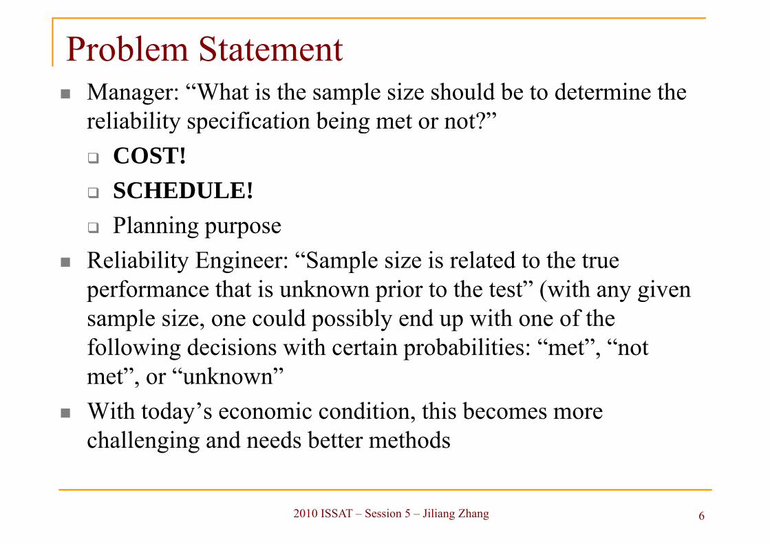
Problem StatementProblem StatementManager: “What is the sample size should be to determine the reliability specification being met or not?”reliability specification being met or not?

COST!SCHEDULE!Planning purpose

Reliability Engineer: “Sample size is related to the true performance that is unknown prior to the test” (with any given sample size, one could possibly end up with one of the following decisions with certain probabilities: “met”, “not met”, or “unknown” With today’s economic condition, this becomes more ychallenging and needs better methods


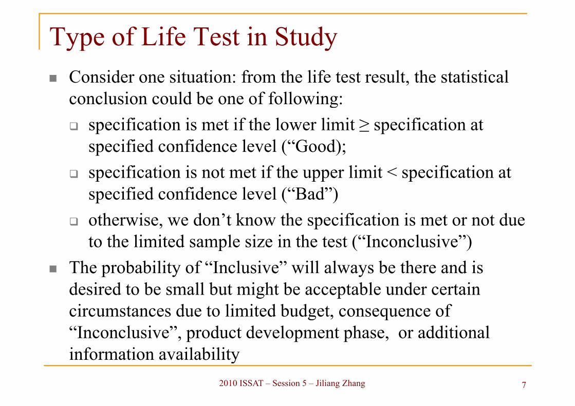
Type of Life Test in StudyType of Life Test in StudyConsider one situation: from the life test result, the statistical conclusion could be one of following:

specification is met if the lower limit ≥ specification at specified confidence level (“Good);specification is not met if the upper limit < specification at p pp pspecified confidence level (“Bad”)otherwise, we don’t know the specification is met or not dueotherwise, we don t know the specification is met or not due to the limited sample size in the test (“Inconclusive”)

The probability of “Inclusive” will always be there and isThe probability of Inclusive will always be there and is desired to be small but might be acceptable under certain circumstances due to limited budget, consequence ofcircumstances due to limited budget, consequence of “Inconclusive”, product development phase, or additional information availability


y7

General MethodologyGeneral MethodologyLink the sample size to the probability of reaching conclusions of “Good” “Bad” and “Inconclusive” if the performance isof Good , Bad , and Inconclusive if the performance is indeed good enough and/or bad enough. Probability of Decision Table:Probability of Decision Table:

Decision Worse-than-ifi ti

Better-than-ifi tispecification

performancespecification performance

“Good” p0GType II Error p1Gp0G p1G

“Inconclusive” p0U p1U

“Bad” p0B p1BType I Error

Note: this is not an acceptance test in which there are only two conclusionscan be drawn: either accept or reject

p0B p1B

can be drawn: either accept or reject

A sample size can be determined if a resulting probability of decision table is acceptable


decision table is acceptable 8

Exponential Distribution Case – CriterionExponential Distribution Case Criterion of Decisions

For a time-censored life test,2T 2T

C i i f d i i i h h l f

222;

12

+

=r

LTm

αχ2

2;11

2

rU

Tmαχ −

=

Criterion of decision with the goal of mG

“Good” or the specification is met if mL1 ≥ mG;“Bad” or the specification is not met if mU1 < mG;“Inconclusive” if mL1 < mG ≤ mU1L1 G ≤ U1.

Define rG be the maximum number of failures that satisfies mL1 ≥ mG, and rB be the minimum number of failures thatmL1 ≥ mG, and rB be the minimum number of failures that satisfies mU1 < mG


d9

Exponential Distribution Case – ProbabilityExponential Distribution Case Probability of Decision Table Calculation

The number of failures within T follows a Poisson distribution. So,

The probability of decision of “Good” is)(

∑−

emT

GrmT

r

The probability of decision of “Bad” is

1,0,!

)|(0

===≤= ∑=

ir

mmmrXPpr

iGiG

The probability of decision of Bad is

1,0,!

)()|( ===≥= ∑

∞

−

ir

emT

mmrXPpmT

r

iBiB

The probability of “Inconclusive” is

!= rBrr

−T T

1,0,!

)()|(

1

1===<<= ∑

−

+=

ir

emT

mmrXrPpB

G

r

rr

mr

iBGiU


Exponential Distribution Case – ExampleExponential Distribution Case ExampleAssume 1 − α = 90%, m0 = mG/2 and m1 = 2mG. Set T/ mG = 7. We , 0 G 1 G Gcan obtain rG = 3 and rB = 11 from the equations in previous slide 6. So, the following probability of decisions table can be obtained from equations in Slide 7:

Decision m0 = mG/2 m1= 2mG

“Good’ 0.1% 53.7%“Inconclusive” 17.4% 46.2%

Note: In this example one may feel the probability of “Inconclusive” when m = 2m

“Bad” 82.5% 0.1%

Note: In this example, one may feel the probability of Inconclusive when m1 = 2mG

is too big. Increasing sample size would reduce this uncertainty. In real case, one can decide to further monitor the performance since this is in the middle of pproduct development , we have additional information, and the consequence of “Inconclusive” may not be that significant.


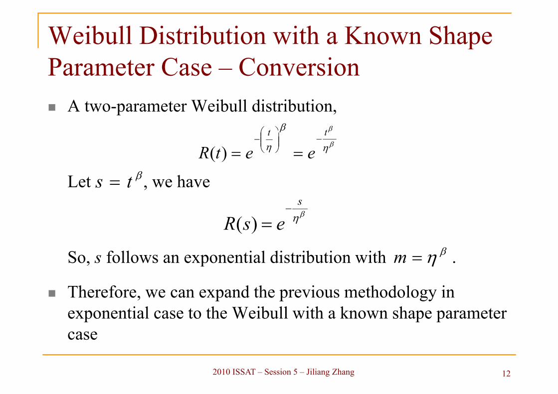
Weibull Distribution with a Known ShapeWeibull Distribution with a Known Shape Parameter Case – Conversion

A two-parameter Weibull distribution, ββ tt ⎞⎛

h

β

β

η

β

ηtt

eetR−⎟⎟

⎠

⎞⎜⎜⎝

⎛−

==)(βLet , we haveβts =

βηs

R−

)(

So, s follows an exponential distribution with .

ηesR =)(βη=mSo, s follows an exponential distribution with .

Therefore, we can expand the previous methodology in

ηm

exponential case to the Weibull with a known shape parameter case


Weibull Distribution Case – Criterion ofWeibull Distribution Case Criterion of Decisions

Let k is the initial number of units

β)( ctkS =k is the initial number of unitstc is predetermined censoring time (k ) i id d l i(k, tc) is considered as a sample size.

For a time-censored life test,

222;

12

+

=r

LS

α

β

χη 2

2;11

2

rU

S

α

β

χη

−

=

Define rG be the maximum number of failures that satisfies ηL1 ≥ ηG and rB the minimum number of failures that satisfies ηU1

22; +rαχ ;

≥ ηG, and rB the minimum number of failures that satisfies ηU1< ηG


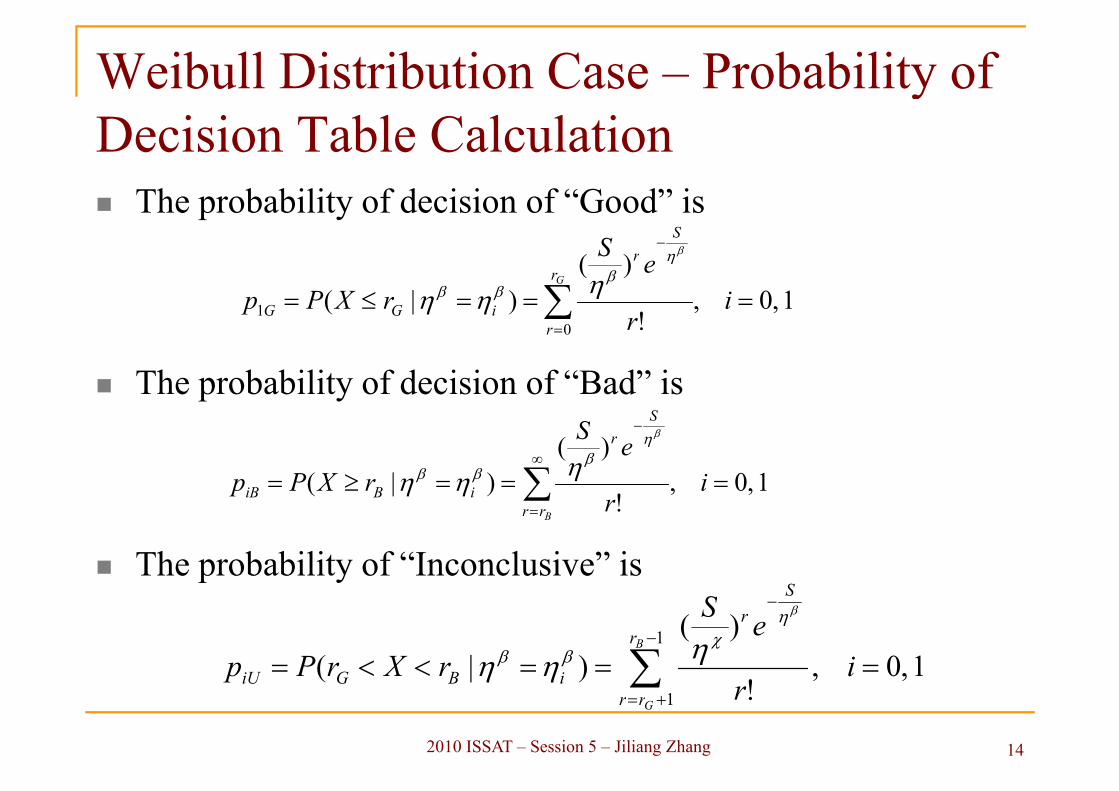
Weibull Distribution Case – Probability ofWeibull Distribution Case Probability of Decision Table Calculation

The probability of decision of “Good” is

)(−

eSS

r βη

1,0,!

)()|(

01 ===≤= ∑

=

ir

erXPp

Gr

riGG

ηβ

ββ ηηη

The probability of decision of “Bad” is

)(−S

Sr βη

1,0,!

)()|( ===≥= ∑

∞

=

ir

eS

rXPpBrr

r

iBiB

ηβ

ββ ηηη

The probability of “Inconclusive” is−

)(S

rS βη

∑−

+=

===<<=1

11,0,

!

)()|(

B

G

r

rr

r

iBGiU ir

eS

rXrPp

βηχ

ββ ηηη


+1Grr

Weibull Distribution Case – ExampleRequired reliability for 25,000 hours is 97.5%. Assume 1 − α = 90%. The time-between-failures follows a two-parameter pWeibull distribution with a known β = 2.0. The required reliability can be converted to required ηG = 157,118 hours or y q ηG ,required = 24,686,000,000. We further assume = /2 and = 2 , which correspond to the reliability of 95.1%

βηGβη0

βηGβη1βηG

and 98.7%, respectively. For tc = 3×25,000 = 75,000 hours and k = 30, we can obtain rG = 3 and rB = 11 from equations in Slide

η1 ηG

10. So, the following probability of decisions table can be obtained from equations in Slide 11:

β βDecision

“Good” 0% 53.4%

βη 0βη1

“Inconclusive” 6.6% 46.6%

“Bad” 93.4% 0%


ConclusionsConclusionsSample size is linked to the probability of decisions or risks of statistical errors or “inconclusive”

Probability of decision table can be used to determine theProbability of decision table can be used to determine the sample size needed

Upper and lower performance as well as values in probability of decision table depends on specific application. Some consideration factors could be

Required reliability or failure consequenceq y qCost of the test and budget availableProduct development phasep pConsequence and the possible action items for “Inconclusive” Additional available information


Additional available information16

life test sample size determination based on probability of decisions

Technology