low-complexity frequency synchronization for wireless ofdm systems
TRANSCRIPT

Low-Complexity Frequency Synchronization forWireless OFDM Systems
PROEFSCHRIFT
ter verkrijging van de graad van doctor aan deTechnische Universiteit Eindhoven, op gezag van de
rector magnificus, prof.dr.ir. C.J. van Duijn, voor eencommissie aangewezen door het College voor
Promoties in het openbaar te verdedigenop maandag 23 november 2009 om 14.00 uur
door
Wu Yan
geboren te Qingdao, China
Dit proefschrift is goedgekeurd door de promotoren:
prof.dr.ir. J.W.M. Bergmansenprof.dr. C.C. Ko
Copromotor:dr. S. Attallah
A catalogue record is available from the Technische Universiteit EindhovenLibrary
Wu, Yan
Low-Complexity Frequency Synchronization for Wireless OFDM Systems /by Wu Yan -Eindhoven : Technische Universiteit Eindhoven, 2009. -Proefschrift. – ISBN: 978-90-386-2068-8NUR 959Subject headings: signal processing \ wireless communications \ frequencysynchronization \ OFDM modulation
c© Copyright 2009 by Wu Yan
All rights reserved. No part of this publication may be reproduced, stored ina retrieval system, or transmitted in any form or by any means, electronic,mechanical, including photocopying , recording, or otherwise, without theprior written permission from the copyright owner.

3
To my wife Liu Ying
and
our little angel who is actively playing in mommy’s womb

4
Samenstelling van de promotiecommissie:
prof.dr.ir. A.C.P.M. Backx, Technische Universiteit Eindhoven, voorzitterprof.dr.ir. J.W.M. Bergmans, Technische Universiteit Eindhoven, promotorprof.dr. C.C. Ko, National University of Singapore, promotordr. S. Attallah, SIM University (UniSIM), copromotorprof.dr.ir. W.C. van Etten, University of Twentedr. G. Leus, Technische Universiteit Delftdr.ir. P.F.M. Smulders, Technische Universiteit Eindhoven

Acknowledgements i
Acknowledgements
First and foremost, I would like to express my sincere gratitude to my mainsupervisor Dr. Samir Attallah. I am grateful to him for introducing me to theNUS-TU/e joint PhD program, for his sustained guidance and encouragementin the past 5 years and for many exciting and enlightening technical discus-sions. I deeply appreciate his understanding of the difficulties I had trying tobalance work and study as a part-time student during my study in Singapore.Besides being an excellent teacher, Samir is always a good friend. I enjoyedmany casual discussions with him on work and life-related matters. I still re-member our shared sympathy on the sending off of Zinedine Zidane in the 2006world cup final. I am also truly grateful to my co-supervisor Prof. dr. ir. JanBergmans. His broad knowledge and deep technical insights have been a con-tinuous source of inspiration. Jan has also shown me the importance of goodscientific writing. I deeply appreciate his most valuable critique, suggestionsand feedback to improve the quality of this thesis and my scientific writing ingeneral. I also very much enjoyed many difficult yet intriguing challenges thathe posed during our discussions. I also would like to thank him for providingme the opportunity to work fulltime in TU/e for my PhD.
I also want to thank a group of wonderful colleagues and friends in Institutefor Infocomm Research (I2R) in Singapore. They are Sumei, Patrick, ChinKeong, Woonhau, Peng Hui, Zhongding, Yuen Chau and many more. Workingwith you guys was a marvelous experience. Specially, I would like to thankSumei for her support, guidance and understanding as a manager and for hervaluable personal advices as a friend. In TU/e, I am also grateful to Prof.Peter Baltus for his expert knowledge in the RF front-end and to Prof. JeanPaul Linnartz for his help on the modeling of antenna mutual coupling andspatial correlation. I would like to acknowledge Yvonne Broers, Anja de Valk-Roulaux and Yvonne van Bokhoven for their kind assistance in administrativematters. I am very grateful to Sjoerd Ypma for meeting me at the railwaystation on a cold winter night on my first day in Eindhoven, and for providingme with so many useful information and tips on the life in the Netherlands.My appreciation goes to the whole SPS group for the pleasant atmospherethey created. I had great fun in the two cycling tours. I am lucky to have fourgreat office mates, Hongming, Wim, Zhangpeng and Hamid. I am indebtedto them for interesting discussions and many good jokes.

ii Acknowledgements
Many thanks go to prof.dr. C.C. Ko, prof.dr.ir. W.C. van Etten, dr. G. Leus,dr.ir. P.F.M. Smulders and prof.dr.ir. A.C.P.M. Backx for being in my doctor-ate committee and for their insightful comments and suggestions.
The love and support I get from my family are beyond what words can de-scribe. I am deeply indebted to my grandma, my parents for their love fromthe first day I came to this world, and for their continuous encouragement,which has been a driving force throughout the years in my study, work anddaily life. I would also like to thank my parents in law for their understand-ing and support. Last and definitely not the least, I would like to thank mywife Liu Ying. She has been most understanding and supportive for my studyand work. I am heartily grateful for her love, for always being by my sideand making me the happiest husband. I will never forget all the sacrifices shemade to help me complete this thesis.
Contents
Acknowledgements i
Summary vii
List of Figures xi
List of Tables xv
List of Abbreviations xvii
List of Symbols xix
1 Introduction 11.1 Overview of Wireless Communication Systems . . . . . . . . . 11.2 Overview of OFDM Systems . . . . . . . . . . . . . . . . . . . 4
1.2.1 Basic Principles of OFDM . . . . . . . . . . . . . . . . . 51.2.2 MIMO-OFDM and Multi-user MIMO-OFDM systems . 10
1.3 Effects of Frequency Synchronization Errors in OFDM Systems 141.4 Status and Challenges in CFO estimation for OFDM systems . 20
1.4.1 CFO estimation for SISO-OFDM systems . . . . . . . . 201.4.2 CFO estimation for MIMO-OFDM systems . . . . . . . 271.4.3 CFO estimation for Multi-user MIMO-OFDM systems . 29
1.5 Outline and Contributions of the Thesis . . . . . . . . . . . . . 291.6 List of Publications by the Author . . . . . . . . . . . . . . . . 31
1.6.1 Journals . . . . . . . . . . . . . . . . . . . . . . . . . . . 311.6.2 Conference Proceedings . . . . . . . . . . . . . . . . . . 32
iv Contents
2 Low-Complexity Blind CFO Estimation for OFDM Systems 332.1 Introduction . . . . . . . . . . . . . . . . . . . . . . . . . . . . . 332.2 Previous Methods . . . . . . . . . . . . . . . . . . . . . . . . . 342.3 Proposed New Factorization Method . . . . . . . . . . . . . . . 372.4 Successive Blind CFO Estimation and Compensation . . . . . . 412.5 Decision-directed Successive Algorithm . . . . . . . . . . . . . . 452.6 Simulation Results . . . . . . . . . . . . . . . . . . . . . . . . . 47
2.6.1 Simulation Results for the New Factorization Method . 482.6.2 Simulation Results for the Successive CFO Estimation
and Compensation Algorithm . . . . . . . . . . . . . . . 512.6.3 Simulation Results for the Decision-directed Algorithm . 53
2.7 Conclusions . . . . . . . . . . . . . . . . . . . . . . . . . . . . . 56
3 Optimal Null Subcarrier Placement for Blind CFO Estima-tion 573.1 Introduction . . . . . . . . . . . . . . . . . . . . . . . . . . . . . 573.2 Placement of Null Subcarriers Based on SNRCFO Maximization 593.3 Placement of Null Subcarriers Based on the Theoretical MSE
Minimization . . . . . . . . . . . . . . . . . . . . . . . . . . . . 693.4 Practical Considerations . . . . . . . . . . . . . . . . . . . . . . 733.5 Simulation Results . . . . . . . . . . . . . . . . . . . . . . . . . 773.6 Conclusion . . . . . . . . . . . . . . . . . . . . . . . . . . . . . 81
4 Clock Signal Generation and Distribution Topologies for MIMOSystems 854.1 Introduction . . . . . . . . . . . . . . . . . . . . . . . . . . . . . 854.2 System Model . . . . . . . . . . . . . . . . . . . . . . . . . . . . 904.3 Power Loss on Microstrip Lines . . . . . . . . . . . . . . . . . . 92
4.3.1 Microstrip Line Analysis Using Quasi-static Method . . 934.3.2 Microstrip Line Analysis using Dispersion Models . . . . 944.3.3 Power Loss Calculation . . . . . . . . . . . . . . . . . . 96
4.4 Power Dissipation for a MIMO Receiver with Four Antennas . 984.4.1 Centralized Generation of GHz Clocks . . . . . . . . . . 984.4.2 Distributed Generation of GHz Clocks . . . . . . . . . . 994.4.3 Centralized RF Processing . . . . . . . . . . . . . . . . . 100
4.5 Comparisons and Discussions . . . . . . . . . . . . . . . . . . . 1014.6 Conclusions . . . . . . . . . . . . . . . . . . . . . . . . . . . . . 105
5 CFO Estimation for MIMO-OFDM Systems 1075.1 Introduction . . . . . . . . . . . . . . . . . . . . . . . . . . . . . 1075.2 System Model . . . . . . . . . . . . . . . . . . . . . . . . . . . . 110

Contents v
5.3 CAZAC Sequences for Joint CFO and Channel Estimation . . 1125.4 MSE Analysis of Channel Estimation with Residual CFO . . . 1175.5 Simulation Results . . . . . . . . . . . . . . . . . . . . . . . . . 1215.6 Effect of Spatial Correlation Related to the Propagation Envi-
ronment . . . . . . . . . . . . . . . . . . . . . . . . . . . . . . . 1235.7 Effect of Mutual Coupling among the Antennas . . . . . . . . . 1295.8 Conclusions . . . . . . . . . . . . . . . . . . . . . . . . . . . . . 134
6 CFO Estimation for Multi-user MIMO-OFDM Uplink UsingCAZAC Sequences 1376.1 Introduction . . . . . . . . . . . . . . . . . . . . . . . . . . . . . 1376.2 System Model . . . . . . . . . . . . . . . . . . . . . . . . . . . . 1416.3 CAZAC Sequences for Multiple CFO’s Estimation . . . . . . . 1436.4 Training Sequence Optimization . . . . . . . . . . . . . . . . . 148
6.4.1 Cost Function Based on SIR . . . . . . . . . . . . . . . 1486.4.2 CFO-Independent Cost Function . . . . . . . . . . . . . 150
6.5 Simulation Results . . . . . . . . . . . . . . . . . . . . . . . . . 1526.6 Conclusions . . . . . . . . . . . . . . . . . . . . . . . . . . . . . 159
7 Conclusions and Future Work 1617.1 Conclusions . . . . . . . . . . . . . . . . . . . . . . . . . . . . . 1617.2 Future Work . . . . . . . . . . . . . . . . . . . . . . . . . . . . 164
References 176
Curriculum vitae 177

vi Contents
Summary vii
Summary
Low-Complexity Frequency Synchronizationfor Wireless OFDM Systems
In the past decade, we have seen a trend in wireless communications fromsupporting only voice and low-rate data services towards supporting high-rate multimedia applications. To support this high demand on data rate,the bandwidth of modern wireless communication systems is normally in theorder of tens of MHz. Because of this large bandwidth, the communicationchannels between the transmitter and the receiver exhibit different responsesat different frequencies, and are called frequency-selective fading channels.The Orthogonal Frequency Division Multiplexing (OFDM) system provides anefficient and robust solution for communication over frequency-selective fadingchannels and has been adopted in various wireless communication standards.The multiple-input and multiple-out (MIMO) OFDM system further increasesthe data rates and robustness of the OFDM system by using multiple transmitand receive antennas. The multi-user MIMO-OFDM system is an extensionof the MIMO-OFDM system to a multi-user context. It enables transmissionand reception of information from multiple users at the same time and in thesame frequency band.
A common drawback of all these wireless OFDM systems is their sensitivity tofrequency synchronization errors in the form of carrier frequency offset (CFO).CFO is an offset between the carrier frequency of the transmitted signal andthe carrier frequency used at the receiver for demodulation. It is caused bythe mismatch between the transmitter and receiver local oscillators and, incase of moving transmitters and/or receivers, also by the Doppler effect ofthe channel. In OFDM systems, CFO causes inter-carrier interference (ICI),which can be several orders larger than the noise sources in the system. Thus,accurate CFO estimation, through frequency synchronization, is essential forensuring adequate performance of OFDM systems. To this end, many CFOestimation and compensation algorithms have been described in the literaturefor a variety of wireless OFDM systems. These algorithms can be broadlydivided into two categories, namely blind algorithms and training-based al-gorithms. For blind CFO estimation algorithms, CFO is estimated using the
viii Summary
statistical properties of the received signal only, without explicit knowledge ofthe transmitted signal. For training-based CFO estimation algorithms, spe-cially designed training signals known to the receiver are transmitted to assistthe receiver in estimating the CFO. A key drawback of blind algorithms istheir high computational complexity. In this thesis, we address this drawbackby developing a particular type of low-complexity blind CFO estimation al-gorithms in the context of single-input single-output (SISO) OFDM systems.For training-based algorithms, the computational complexity is normally lowbecause training sequences can be designed to limit the required computationsat the receiver. A key drawback of training-based algorithms is the trainingoverhead from the transmission of training sequences, as it reduces the effec-tive data throughput of the system. Comparing to SISO-OFDM systems, thetraining overhead for MIMO-OFDM systems is even larger. To address thisdrawback, in this thesis, we propose an efficient training sequence design forMIMO-OFDM systems, which has low training overhead and at the same timepermits low-complexity maximum-likelihood joint CFO and channel estima-tion.
This thesis can be divided into three parts covering different wireless OFDMsystems. In the first part, consisting of Chapters 2 and 3, we study low-complexity blind CFO estimation algorithms in SISO-OFDM systems. Inthe second part, consisting of Chapters 4 and 5, we study CFO estimationfor MIMO-OFDM systems and propose low-overhead training sequences thatalso enable low-complexity joint CFO and channel estimation. In the thirdpart, consisting of Chapter 6, we propose a low-complexity CFO estimationalgorithm in the uplink of multi-user MIMO-OFDM systems using constantamplitude zero autocorrelation (CAZAC) training sequences.
In Chapter 2 and 3 of the thesis, we study how to reduce the computationalcomplexity of a very popular blind CFO estimation algorithm that exploits nullsubcarriers. These are subcarriers at both ends of the allocated spectrum thatare left empty and used as guard bands. Existing algorithms exploiting nullsubcarriers require finding roots of a cost function, which is a high-order poly-nomial. The computational complexity of these algorithms is thus high. Toreduce the computational complexity, we derive a closed-form CFO estimatorby using a low-order Taylor series approximation of the original cost function.We also propose a successive CFO estimation and compensation algorithmto limit the performance degradation due to the Taylor series approximation.The computational complexity of the proposed algorithms is significantly lowerthan that of existing algorithms, while performance is comparable for practicalCFO values. The best null subcarrier placement that maximizes the signal to
Summary ix
noise ratio (SNR) of the CFO estimation is also studied. We show that tomaximize the SNR of CFO estimation, the null subcarriers should be evenlyspaced in an OFDM symbol. Moreover, we prove that this SNR-maximizingnull subcarrier placement also minimizes the theoretical mean square error(MSE), which is an accurate linear approximation of the actual MSE in highSNR regions, of the CFO estimation.
In MIMO systems, there are multiple radio frequency front-ends, which requiremultiple clock signals, at both the transmitter and the receiver. Accordingly,there are different clock signal generation and distribution topologies speci-fying how clock signals are generated and distributed to different front-ends.It is of practical importance to study the pros and cons of these topologiesas they directly affect the design of the front-end architecture and the subse-quent digital signal processing algorithms. To our best knowledge, this typeof study has not been reported in the literature and is presented in Chapter4. We first develop a general mathematical model to calculate the power dis-sipations for different topologies. Using this model, we show that for a typicalwireless LAN system setup studied in this thesis, centralized clock generation,where clock signals are generated centrally using one frequency synthesizer,dissipates less power compared to distributed clock generation, where multi-ple frequency synthesizers are used. Compared to SISO-OFDM systems, thetraining for CFO and channel estimation for MIMO-OFDM systems requiressignificantly larger overhead due to the use of multiple antennas at the trans-mitter and the receiver. To mitigate the reduction in the useful data through-put due to training, it is important to find a training sequence that is shorterand at the same time still permits good performance and low computationalcomplexity. In Chapter 5, we propose an efficient (low-overhead) trainingsequence design using constant amplitude zero autocorrelation (CAZAC) se-quences and study the corresponding joint CFO and channel estimation inMIMO-OFDM systems. We show that using the proposed training sequence,the CFO estimate can be obtained using low-complexity correlation operationsand the performance approaches the Cramer-Rao Bound. Simultaneously, amaximum-likelihood channel estimate can be obtained with simple matrixmultiplications. Moreover, the training overhead is significantly reduced com-pared to existing frequency-domain training sequences. In Chapter 5, we alsostudy how the spatial correlation and antenna mutual coupling affect the per-formance of the CFO estimation in MIMO systems.
In the uplink of multi-user MIMO-OFDM systems, there are multiple CFO val-ues between the centralized clock at the receiver (base station) and the clocksof different users. Maximum-likelihood estimator for these multiple CFO val-

x Summary
ues is not practical because it requires a complexity that grows exponentiallywith the number of users. Some low-complexity methods have been proposedin the literature based on adaptive searching algorithms and importance sam-pling. However, the complexity, though reduced, is still relatively high forpractical implementations. To further reduce the computational complexity,in Chapter 6, we propose a low-complexity sub-optimal CFO estimation algo-rithm using CAZAC training sequences. Using the proposed algorithm, theCFO of each user can be estimated using simple correlation operations and thecomputational complexity grows only linearly with the number of users. Wealso show that multiple CFO values in the uplink cause interference in the CFOestimation of different users using the proposed low-complexity algorithm. Toreduce this interference, we formulate a training sequence optimization prob-lem and find the CAZAC sequences that maximize the signal to interferenceratio.
List of Figures
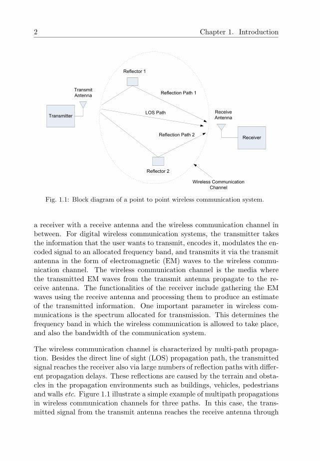
1.1 Block diagram of a point to point wireless communication sys-tem. . . . . . . . . . . . . . . . . . . . . . . . . . . . . . . . . . 2
1.2 Demand for data rate in WLAN systems. . . . . . . . . . . . . 41.3 Block diagram of an OFDM system. . . . . . . . . . . . . . . . 51.4 Amplitude spectra of subcarriers 6 to 10 for an OFDM system
with 16 subcarriers. . . . . . . . . . . . . . . . . . . . . . . . . 91.5 A block diagram of a MIMO-OFDM system. . . . . . . . . . . 131.6 Illustration of a multi-user MIMO-OFDM system. . . . . . . . 131.7 An OFDM receiver with frequency synchronization. . . . . . . 151.8 The packet structure of a IEEE 802.11g data packet. . . . . . 171.9 Effects of CFO in OFDM systems . . . . . . . . . . . . . . . . 181.10 SINR of the received signal in OFDM systems for different CFO
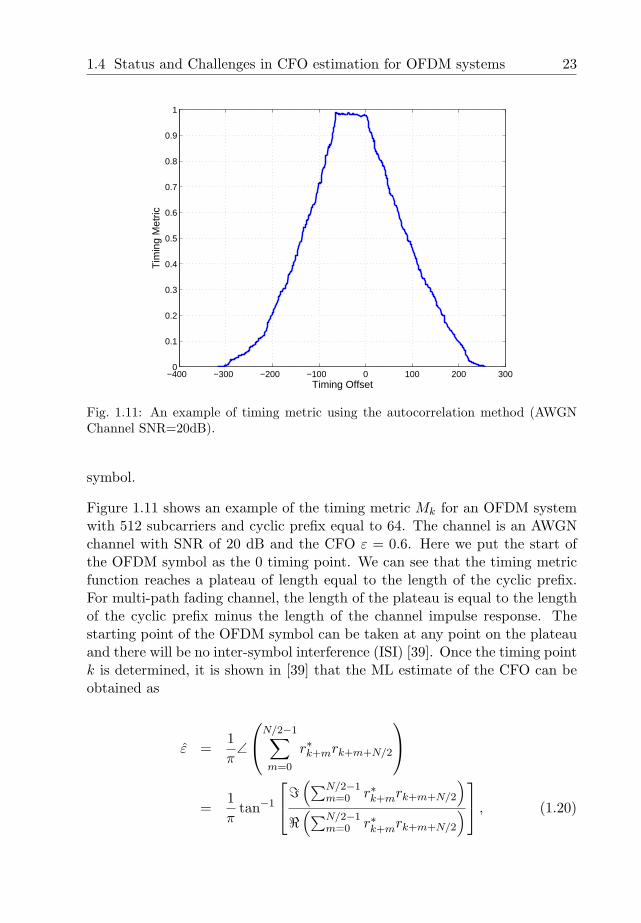
values. . . . . . . . . . . . . . . . . . . . . . . . . . . . . . . . 191.11 An example of timing metric using the autocorrelation method
(AWGN Channel SNR=20dB). . . . . . . . . . . . . . . . . . . 231.12 Typical spectrum of an OFDM system with guard bands (null
subcarriers). . . . . . . . . . . . . . . . . . . . . . . . . . . . . 27
2.1 MSE of CFO estimation using the new method (−0.25ω ≤ φ0 ≤0.25ω). . . . . . . . . . . . . . . . . . . . . . . . . . . . . . . . 48
2.2 MSE of CFO estimation using the new method for evenly placednull subcarriers (−0.5ω ≤ φ0 ≤ 0.5ω). . . . . . . . . . . . . . . 49
2.3 SER with CFO estimation using the new method for evenlyplaced null subcarriers using QPSK modulation (−0.5ω ≤ φ0 ≤0.5ω). . . . . . . . . . . . . . . . . . . . . . . . . . . . . . . . . 50
xii List of Figures
2.4 MSE of CFO estimation using the successive CFO estimationand compensation algorithm (−0.7ω ≤ φ0 ≤ 0.7ω). . . . . . . 52
2.5 SER with CFO estimation using the successive CFO estimationand compensation algorithm for QPSK modulation(−0.7ω ≤φ0 ≤ 0.7ω). . . . . . . . . . . . . . . . . . . . . . . . . . . . . . 52
2.6 Convergence behavior of the successive algorithm (φ0 = 0.7ω,SNR=20dB). . . . . . . . . . . . . . . . . . . . . . . . . . . . . 53
2.7 CFO estimation using the previous method with Q = 1 and thesuccessive algorithm (−0.7ω ≤ φ0 ≤ 0.7ω). . . . . . . . . . . . 54
2.8 SER with CFO estimation using the previous method withQ = 1 and the successive algorithm with QPSK modulation(−0.7ω ≤ φ0 ≤ 0.7ω). . . . . . . . . . . . . . . . . . . . . . . . 54
2.9 CFO estimation using decision-directed algorithm with Q = 1(−0.25ω ≤ φ0 ≤ 0.25ω). . . . . . . . . . . . . . . . . . . . . . . 55
3.1 Illustration of the placement of 3 null-subcarriers. . . . . . . . 643.2 Comparison between the theoretical MSE and the MSE ob-
tained from simulations. . . . . . . . . . . . . . . . . . . . . . 783.3 MSE performance of the CFO estimation using different null
subcarrier placements. . . . . . . . . . . . . . . . . . . . . . . 793.4 SER performance with CFO estimation using different null sub-
carrier placements (QPSK modulation). . . . . . . . . . . . . . 803.5 MSE performance of the CFO estimation for OFDM systems
with guard bands and different number of optimally-placed freenull subcarriers. . . . . . . . . . . . . . . . . . . . . . . . . . . 80
4.1 A typical MIMO receiver with Nr RF front-ends. . . . . . . . . 864.2 A zero-IF receiver RF front-end. . . . . . . . . . . . . . . . . . 874.3 Receiver with centralized generation of GHz clock signals and
distributed frequency down-conversion. . . . . . . . . . . . . . . 884.4 Receiver with distributed generation of GHz clock signals and
distributed frequency down-conversion. . . . . . . . . . . . . . . 894.5 Receiver with centralized RF processing. . . . . . . . . . . . . 894.6 Geometric structure of a microstrip transmission line. . . . . . 924.7 Power loss of microstrip lines using FR4 laminates. . . . . . . . 974.8 Power loss of microstrip lines using the RT/duroidr 5870 high
frequency laminates for millimeter wave frequencies. . . . . . . 984.9 Power dissipation of different clock signal generation and dis-
tribution topologies for the 2.4 GHz band. . . . . . . . . . . . . 1024.10 Power dissipation of different clock signal generation and dis-
tribution topologies for the 5 GHz band. . . . . . . . . . . . . . 102
List of Figures xiii
4.11 Power dissipation of different clock signal generation and dis-tribution topologies for the 60 GHz band. . . . . . . . . . . . . 103
5.1 MSE of CFO estimation using the proposed training sequence. 1225.2 Performance of channel estimation using the proposed CAZAC
sequence in the presence of residual CFO. . . . . . . . . . . . . 1235.3 Received signal for a two-element antenna array spaced d for a
plane wave impinging at angle θ. . . . . . . . . . . . . . . . . . 1255.4 Correlation coefficients for different angular spreads for a fixed
mean AOA of 0o. . . . . . . . . . . . . . . . . . . . . . . . . . . 1285.5 Correlation coefficients for different mean AOA values for a
fixed angular spread of 20o. . . . . . . . . . . . . . . . . . . . . 1295.6 MSE of CFO estimation for different angular spreads for a fixed
mean AOA of 0o. . . . . . . . . . . . . . . . . . . . . . . . . . . 1305.7 MSE of CFO estimation for different mean AOA values for a
fixed angular spread of 20o. . . . . . . . . . . . . . . . . . . . . 1305.8 Effective spatial correlation due to coupling for two λ/2 dipole
antennas with Zload = Z∗s . . . . . . . . . . . . . . . . . . . . . . 1335.9 Power loss due to coupling for two λ/2 dipole antennas with
Zload = Z∗s . . . . . . . . . . . . . . . . . . . . . . . . . . . . . . 1335.10 Effects of mutual coupling on the performance of CFO estimation.134
6.1 Illustration of the multi-user MIMO-OFDM system. . . . . . . 1386.2 MSE of CFO estimation using N = 32 Chu sequences and IEEE
802.11n STF for uniform power delay profile. . . . . . . . . . . 1556.3 Comparison of CFO estimation using N = 31 Chu sequences
and m sequence for uniform power delay profile. . . . . . . . . 1556.4 Comparison of SER using QPSK modulation for CFO estima-
tion using different sequences for uniform power delay profile. 1566.5 Comparison of CFO estimation using different N = 36 CAZAC
sequences for L = 18 channel for uniform power delay profile. 1576.6 Comparison of CFO estimation using different length of optimal
Chu sequences for L = 18 channel for uniform power delayprofile. . . . . . . . . . . . . . . . . . . . . . . . . . . . . . . . 158
6.7 Comparison of useful signal and interference power for differ-ent sequence lengths using Chu sequences (uniform power delayprofile). . . . . . . . . . . . . . . . . . . . . . . . . . . . . . . . 159

xiv List of Figures
List of Tables
2.1 Summary of the closed-form CFO estimator using the new fac-torization method. . . . . . . . . . . . . . . . . . . . . . . . . . 41
2.2 Summary of the proposed successive CFO estimation and com-pensation algorithm. . . . . . . . . . . . . . . . . . . . . . . . . 44
2.3 Summary of the proposed decision-directed successive CFO es-timation and compensation algorithm. . . . . . . . . . . . . . . 47
3.1 Heuristic null subcarrier placement when N is not divisible byd (nl > nu). . . . . . . . . . . . . . . . . . . . . . . . . . . . . . 68
3.2 Heuristic null subcarrier placement for d=4 to 11 for N=64OFDM systems . . . . . . . . . . . . . . . . . . . . . . . . . . . 68
3.3 SNR-optimal free null subcarrier placement for IEEE 802.11asystems . . . . . . . . . . . . . . . . . . . . . . . . . . . . . . . 75
4.1 Parameters of microstrip lines used. . . . . . . . . . . . . . . . 97
5.1 Extra MSE caused by residual CFO for different training se-quence lengths and different number of receive antennas . . . . 121
6.1 Number of possible Frank-Zadoff and Chu sequences for differ-ent sequence lengths. . . . . . . . . . . . . . . . . . . . . . . . . 151

xvi List of Tables

List of Abbreviations
3GPP: 3rd Generation Partnership Project3GPP-LTE: 3rd Generation Partnership Project-Long Term EvolutionADC: Analog to Digital ConverterAGC: Automatic Gain ControllerASA: Adaptive Simulated AnnealingAWGN: Additive White Gaussian NoiseBER: Bit Error RateBPF: Band Pass FilterBPSK: Binary Phase Shift KeyingCAZAC: Constant Amplitude Zero AutoCorrelationCDMA: Code Division Multiple AccessCRB: Cramer-Rao BoundCFO: Carrier Frequency OffsetCP: Cyclic PrefixDAB: Digital Audio BroadcastingDFT: Discrete Fourier TransformDVB: Digital Video BroadcastingEM: ElectromagneticEMF: Electromagnetic FieldsFDM: Frequency Division MultiplexingFIR: Finite Impulse ResponseFFT: Fast Fourier TransformGSM: Global System for Mobile communicationsICI: Inter-Carrier InterferenceIDFT: Inverse Discrete Fourier Transform

xviii List of Abbreviations
IEEE: Institute of Electrical and Electronics EngineersIFFT: Inverse Fast Fourier TransformISI: Inter-Symbol InterferenceLAN: Local Area NetworkLNA: Low Noise AmplifierLO: Local OscillatorLOS: Line of SightLPF: Low Pass FilterMAI: Multiple Access InterferenceMbps: Megabits per secondMEMS: Micro-Electro-Mechanical SystemsML: Maximum LikelihoodMSE: Mean Square ErrorMIMO: Multiple Input Multiple OutputOFDM: Orthogonal Frequency Division MultiplexingOFDMA: Orthogonal Frequency Division Multiple AccessPAS: Power Angular SpectrumPAE: Power Added EfficiencyPAPR: Peak to Average Power RatioPDP: Power Delay Profileppm: parts per millionQAM: Quadrature Amplitude ModulationQPSK: Quadrature Phase Shift KeyingRF: Radio FrequencySER: Symbol Error RateSIR: Signal to Interference RatioSINR: Signal to Interference and Noise RatioSISO: Single Input Single OutputSNR: Signal to Noise RatioSTF: Short Training FiledTEM: Transverse Electro MagneticWiMax: Worldwide Interoperability for Microwave AccessWLAN: Wireless Local Area Network
List of Symbols
∠: angle of a complex numberε: carrier frequency offset normalized with subcarrier spacingε: estimate of the carrier frequency offset ε
γ: signal to noise ratioλ: wavelength of the signalφ: angular carrier frequency offset normalized with subcarrier
spacingφ: estimate of the angular carrier frequency offset φ
σ2s : variance of transmitted digital data symbols
σ2n: variance of the AWGN noise
c: speed of lightEs: average energy of a digital data symbolE: diagonal carrier frequency offset matrixfc: carrier frequency of the signal=: imaginary part of a complex numberI: identity matrixIn: identity matrix of size n× n
N0: power spectrum density of the AWGN noiseNg: length of the cyclic prefix<: real part of a complex numbertr: trace of a matrixW: IDFT matrixwH
i : ith row of the DFT matrix
xx List of Symbols
• Symbols for single-input single-output (SISO) OFDM systems:
d: number of null subcarriers in an OFDM symbolH: diagonal frequency-domain channel matrixHk: diagonal frequency-domain channel matrix for the kth OFDM
symbolICIkli(ε): inter-carrier interference on subcarrier li in the kth OFDM sym-
bol due to a carrier frequency offset of εK: number of OFDM symbols used for carrier frequency offset es-
timationl: vector containing the indices of all null subcarriersN : number of subcarriers in an OFDM symbolP : number of data subcarriers in an OFDM symbolQ: number of terms used in the Taylor series expansionr: received time-domain OFDM symbolrcp: received time-domain OFDM symbol before removing cyclic
prefixrk: kth received time-domain OFDM symbols: transmitted frequency-domain OFDM symbolsk: kth transmitted frequency-domain OFDM symbolSNRCFO: SNR of carrier frequency offset estimationTk: carrier frequency offset compensation matrix for the kth iterationx: transmitted time-domain OFDM symbolxcp: transmitted time-domain OFDM symbol after appending cyclic
prefixy: frequency-domain received OFDM symbolyk
li: frequency-domain received signal on subcarrier li in the kth
OFDM symbol
• Symbols for multiple-input multiple-output (MIMO) OFDM systems:
φd: residual carrier frequency offset after compensationρm,n: correlation coefficient between antennas m and n
Ctx: mutual coupling matrix of all transmit antennasCrx: mutual coupling matrix of all receive antennasH: MIMO channel matrix in flat fading channelsHiid: MIMO channel matrix in flat fading channel assuming all ele-
ments are identically and independently distributed
List of Symbols xxi
H(k): frequency-domain MIMO channel matrix on subcarrier k in aMIMO-OFDM system
Hi,j(k): frequency-domain channel response on subcarrier k between thejth transmit antenna and the ith receive antenna
H: (N×nt)×nr time-domain channel matrix containing the chan-nel impulse responses for all transmit and receive antenna pairs
H: N×nr time-domain channel matrix simplified from H assumingCAZAC training sequences
hi,j : N × 1 vector consisting of the L× 1 channel impulse responsevector between the jth transmit antenna and the ith receiveantenna and a (N − L)× 1 zero vector
hτi,j : vector obtained by circularly shifting hi,j τ elements downwards
hi,j(k): kth tap of the channel impulse response between the jth trans-mit antenna and the ith receive antenna
IL: first L rows of an N ×N identity matrixIL: last N − L rows of an N ×N identity matrixJ0: Bessel function of the first kind and order 0L: number of multipath components in the impulse response of
the channelN : AWGN noise matrix for all the receive antennasN : length of one period of the training sequencent: number of transmit antennasnr: number of receive antennasPAS(θ): power angular spectrum at an angle θ
R: Received signal matrix from all receive antennasRtx: correlation matrix of all transmit antennasRrx: correlation matrix of all receive antennasRr: covariance matrix of the received signalSm: an N ×N circulunt matrix with the first column equal to the
training sequence of the mth transmit antennaS: Matrix containing circulunt training matrices from all transmit
antennasZs: self impedance of the antennaZm: mutual impedance between the antennasZload: loading impedance of the antenna
xxii List of Symbols
• Symbols for power dissipation calculations for different clock signal gen-eration and distribution topologies:
αc: conductor loss of the microstrip lineαd: dielectric loss of the microstrip lineε: dielectric constant of the dielectric substrateεe: effective dielectric constant of the dielectric substrateεe(f): frequency dependent effective dielectric constantµ0: permeability of vacuum, µ0 = 4π × 10−7H/mρ: resistivity of the metal conductor strip material used in the
microstrip lineb: thickness of the dielectric substrate used in the microstrip lineNfs: number of frequency synthesizersNam: number of amplifiersPam: power dissipation of an amplifierPfs: power dissipation of a frequency synthesizerPin: input power of an amplifierPLO: clock signal power at the output of the local oscillatorPout: output power of an amplifierPsp: power loss of the RF splitterPtl: power to compensate the propagation loss of RF signals on the
transmission lineRs: surface resistance of the metal conductor stript: thickness of the metal conductor striptan δ: loss tangent of the dielectric material used in the microstrip
lineW : width of the metal conductor stripWe: effective width of the metal conductor strip considering finite
thickness of the stripZ0: characteristic impedance of the transmission lineZ0e: effective characteristic impedance considering finite thickness
of the stripZ0e(f): frequency dependent effective characteristic impedance consid-
ering finite thickness of the strip
Chapter 1Introduction
In this chapter, we first provide an overview of the wireless communicationsystem and the characteristics of the wireless communication channel. Wethen describe the Orthogonal Frequency Division Multiplexing (OFDM) sys-tem and show its numerous advantages that have made it one of the mostwidely adopted systems for wireless communications. We also briefly intro-duce the Multiple Input Multiple Output (MIMO) OFDM system and themulti-user MIMO-OFDM system, which uses OFDM technology in a multi-antenna and multi-user context to further increase the achievable data ratesin wireless channels. The detrimental effect of frequency synchronization errorin the form of carrier frequency offset (CFO) on the performance of OFDMsystems is described next. We show that to guarantee good performance ofOFDM systems, the CFO must be accurately estimated and compensated. Wethen present a literature review on the frequency synchronization, includingCFO estimation and compensation, for different OFDM systems and high-light specific challenges, which motivate the research work in this thesis. Thischapter concludes by a description of the outline of and contributions in thefollowing chapters of this thesis.
1.1 Overview of Wireless Communication Systems
Figure 1.1 shows a brief block diagram of a point to point wireless communi-cation system. The system consists of a transmitter with a transmit antenna,
2 Chapter 1. Introduction
Transmit
Antenna
Receive
Antenna
Reflector 1
Reflector 2
LOS Path
Reflection Path 1
Reflection Path 2
Wireless Communication
Channel
Receiver
Transmitter
Fig. 1.1: Block diagram of a point to point wireless communication system.
a receiver with a receive antenna and the wireless communication channel inbetween. For digital wireless communication systems, the transmitter takesthe information that the user wants to transmit, encodes it, modulates the en-coded signal to an allocated frequency band, and transmits it via the transmitantenna in the form of electromagnetic (EM) waves to the wireless commu-nication channel. The wireless communication channel is the media wherethe transmitted EM waves from the transmit antenna propagate to the re-ceive antenna. The functionalities of the receiver include gathering the EMwaves using the receive antenna and processing them to produce an estimateof the transmitted information. One important parameter in wireless com-munications is the spectrum allocated for transmission. This determines thefrequency band in which the wireless communication is allowed to take place,and also the bandwidth of the communication system.
The wireless communication channel is characterized by multi-path propaga-tion. Besides the direct line of sight (LOS) propagation path, the transmittedsignal reaches the receiver also via large numbers of reflection paths with differ-ent propagation delays. These reflections are caused by the terrain and obsta-cles in the propagation environments such as buildings, vehicles, pedestriansand walls etc. Figure 1.1 illustrate a simple example of multipath propagationsin wireless communication channels for three paths. In this case, the trans-mitted signal from the transmit antenna reaches the receive antenna through
1.1 Overview of Wireless Communication Systems 3
both the LOS path and the reflection path 1 and 2 from reflector 1 and 2. Dueto the different delays of these propagations paths, the receive antenna willreceive multiple versions of the transmitted signal at slightly different times.In this case, the overall channel can be modeled as the summation of differentchannel components from different propagation paths [1] [2]. The maximumdelay spread of the channel is defined as the difference between the maximumand the minimum delays among different propagation paths. As each pathcomponent has randomly distributed amplitude and phase over time, the am-plitude and phase of the overall channel may experience rapid fluctuationsover a short period of time. This type of channel is called fading channel.
In digital communications, the digital information is mapped to analog wave-forms suitable for transmission over a communication channel using a digitalmodulator [3]. Normally, the digital modulator takes blocks of k binary bitsand maps them to one of M = 2k deterministic analog waveforms. Each blockof k binary bits is called a digital data symbol, while the duration of the analogwaveform corresponds to a digital data symbol is called the symbol duration.When the bandwidth of the system is small, the symbol duration is usuallymuch larger than the maximum delay spread of the channel. In this case, thegain (including both the amplitude and phase) of the overall fading channelcan be modeled as a scalar random variable in the time domain. In the fre-quency domain, this type of channel has a constant (flat) frequency responseover the transmission band and hence, is also called flat fading channel. Whenthe bandwidth of the system is large, the symbol duration is smaller than themaximum delay spread of the channel. In this case, the channel can be viewedas a finite impulse response (FIR) filter with multiple nonzero taps and eachtap is modeled as a random variable. In the frequency domain, the channelresponses at different frequencies in the transmission band are different. Thistype of fading channel is called frequency selective fading channel. In the timedomain, the frequency selective fading channel causes inter-symbol interfer-ence (ISI) in the received signal, which can significantly degrade the systemperformance.
In the past few decades, wireless communication technology has evolved enor-mously, from expensive and exclusive professional (e.g. military) equipmentto today’s omnipresent low-cost consumer systems such as Global System forMobile communications (GSM), Bluetooth, and wireless local area networks(WLAN). We also see a trend in wireless technology from supporting only voiceand low-rate data services towards supporting high-rate multimedia applica-tions. For example, as shown in Figure 1.2, in well under a decade, WLANtechnology has evolved from the first IEEE 802.11b system supporting a peak
4 Chapter 1. Introduction
WLAN Data Rates in Mbit/s
10
100
1,000
10,000
802.11
802.11 b
802.11 a/g
802.11n
2000 2005 2010
802.11 VHT
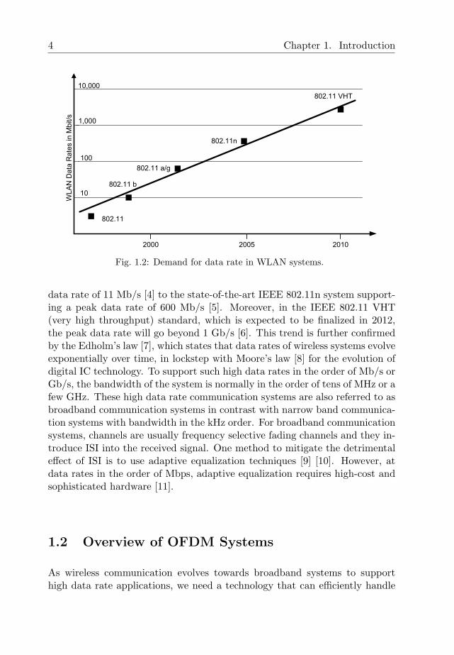
Fig. 1.2: Demand for data rate in WLAN systems.
data rate of 11 Mb/s [4] to the state-of-the-art IEEE 802.11n system support-ing a peak data rate of 600 Mb/s [5]. Moreover, in the IEEE 802.11 VHT(very high throughput) standard, which is expected to be finalized in 2012,the peak data rate will go beyond 1 Gb/s [6]. This trend is further confirmedby the Edholm’s law [7], which states that data rates of wireless systems evolveexponentially over time, in lockstep with Moore’s law [8] for the evolution ofdigital IC technology. To support such high data rates in the order of Mb/s orGb/s, the bandwidth of the system is normally in the order of tens of MHz or afew GHz. These high data rate communication systems are also referred to asbroadband communication systems in contrast with narrow band communica-tion systems with bandwidth in the kHz order. For broadband communicationsystems, channels are usually frequency selective fading channels and they in-troduce ISI into the received signal. One method to mitigate the detrimentaleffect of ISI is to use adaptive equalization techniques [9] [10]. However, atdata rates in the order of Mbps, adaptive equalization requires high-cost andsophisticated hardware [11].
1.2 Overview of OFDM Systems
As wireless communication evolves towards broadband systems to supporthigh data rate applications, we need a technology that can efficiently handle
1.2 Overview of OFDM Systems 5
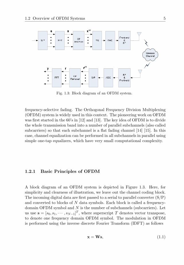
Fig. 1.3: Block diagram of an OFDM system.
frequency-selective fading. The Orthogonal Frequency Division Multiplexing(OFDM) system is widely used in this context. The pioneering work on OFDMwas first started in the 60’s in [12] and [13]. The key idea of OFDM is to dividethe whole transmission band into a number of parallel subchannels (also calledsubcarriers) so that each subchannel is a flat fading channel [14] [15]. In thiscase, channel equalization can be performed in all subchannels in parallel usingsimple one-tap equalizers, which have very small computational complexity.
1.2.1 Basic Principles of OFDM
A block diagram of an OFDM system is depicted in Figure 1.3. Here, forsimplicity and clearness of illustration, we leave out the channel coding block.The incoming digital data are first passed to a serial to parallel converter (S/P)and converted to blocks of N data symbols. Each block is called a frequency-domain OFDM symbol and N is the number of subchannels (subcarriers). Letus use s = [s0, s1, · · · , sN−1]T , where superscript T denotes vector transpose,to denote one frequency domain OFDM symbol. The modulation in OFDMis performed using the inverse discrete Fourier Transform (IDFT) as follows
x = Ws, (1.1)
6 Chapter 1. Introduction
where W denotes the N ×N IDFT matrix, with the (m, n)th element givenby
Wm,n =1√N
exp(j2π
mn
N
).
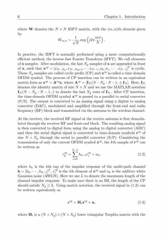
In practice, the IDFT is normally performed using a more computationallyefficient method, the inverse fast Fourier Transform (IFFT). We call elementsof x samples. After modulation, the last Ng samples of x are appended in frontof x, such that xcp = [xN−Ng , xN−Ng+1, · · ·xN−1, x0, x1, · · · , xN−1]T is cyclic.These Ng samples are called cyclic prefix (CP) and xcp is called a time domainOFDM symbol. The process of CP insertion can be written in an equivalentmatrix form as xcp = Acpx, where Acp = [IN (N−Ng : N−1, :); IN ]. Here, IN
denotes the identity matrix of size N ×N and we use the MATLAB notationIN (N −Ng : N − 1, :) to denote the last Ng rows of IN . After CP insertion,the time-domain OFDM symbol xcp is passed to a parallel to serial converter(P/S). The output is converted to an analog signal using a digital to analogconverter (DAC), modulated and amplified through the front-end and radiofrequency (RF) block and transmitted via the antenna to the wireless channel.
At the receiver, the received RF signal at the receive antenna is first demodu-lated through the receiver RF and front-end block. The resulting analog signalis then converted to digital form using the analog to digital converter (ADC)and then the serial digital signal is converted to time-domain symbols rcp ofsize N + Ng through the serial to parallel converter (S/P). Considering thetransmission of only the current OFDM symbol xcp, the kth sample of rcp canbe written as
rcpk =
L−1∑
i=0
hk−ixcpi + nk, (1.2)
where hk is the kth tap of the impulse response of the multi-path channelh = [h0, · · · , hL−1]T , xcp
i is the ith element of xcp and nk is the additive whiteGaussian noise (AWGN). Here we use L to denote the maximum length of thechannel impulse response. To make sure there is no ISI, the length of the CPshould satisfy Ng ≥ L. Using matrix notation, the received signal in (1.2) canbe written equivalently as
rcp = Htxcp + n, (1.3)
where Ht is a (N + Ng)× (N + Ng) lower triangular Toeplitz matrix with the
1.2 Overview of OFDM Systems 7
first column given by [h0, h1, · · · , hL−1, 0, · · · , 0]T as shown below
Ht =
h0 0 · · · 0 · · · 0 0h1 h0 · · · 0 · · · 0 0...
.... . .
.... . .
......
hL−1 hL−2 · · · h0 · · · 0 0...
.... . .
.... . .
......
0 0 · · · 0 · · · h0 00 0 · · · 0 · · · h1 h0
.
At the receiver, the first Ng samples of rcp due to the cyclic prefix are removed,which is indicated by the CP removal block in Figure 1.3. Again this can bewritten in matrix form as r = Dcprcp, where Dcp = [0N×Ng , IN ] with 0N×Ng
denotes a matrix of size N ×Ng whose elements are all 0. Hence, we have thereceived time-domain signal after CP removal given by
r = DcpHtAcpWs + n
= HcWs + n, (1.4)
where Hc = DcpHtAcp. Notice that the effects of CP insertion, channelconvolution and CP removal are combined into a single matrix Hc. It can beeasily shown that Hc is an N ×N circulant matrix given by
Hc =
h0 0 · · · 0 · · · h2 h1
h1 h0 · · · 0 · · · h3 h2...
.... . .
.... . .
......
hL−1 hL−2 · · · h0 · · · 0 0...
.... . .
.... . .
......
0 0 · · · 0 · · · h0 00 0 · · · 0 · · · h1 h0
.
Next the time-domain signal r is transformed to the frequency domain using
8 Chapter 1. Introduction
an N -point FFT. The frequency-domain received signal can be written as
y = WHr = WHHcWs + WHn,
where WH is an N ×N DFT matrix and superscript H denotes matrix Her-mitian. Since Hc is a circulant matrix, it can be diagonalized by the IDFTmatrix as follows
Hc = WHWH ,
where H is a diagonal matrix given by H = diag(WHhc) and hc is the firstcolumn of Hc . In other words, the diagonal elements of H are the DFT of thechannel impulse response h and can be interpreted as the channel frequencyresponses on N subchannels (subcarriers). Using this property, we can re-writethe frequency domain received signal as
y = WHHcWs + WHn = WH(WHWH
)Ws + WHn
= Hs + n′, (1.5)
where n′ is the frequency domain noise term, which is also Gaussian distributedwith zero mean and has the same variance as n. Because H is a diagonalmatrix, we see that different subcarriers are perfectly decoupled after the FFToperation and the frequency selective fading channel can be equalized using asimple one-tap equalizer on each subcarrier individually.
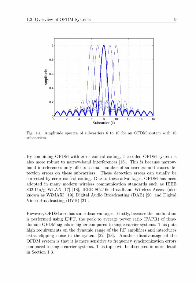
By way of illustration, the amplitude spectra of subcarriers 6 to 10 for anOFDM system with N = 16 are sketched in Figure 1.4. We can see thatthe spectra of different subcarriers are overlapping. At the center of eachsubcarrier, the signals from the other subcarriers are 0. This means thatin OFDM systems, different subcarriers are orthogonal at the center of eachsubcarrier, although their spectra are overlapping.
From above, we can see that in OFDM systems, the frequency selective fadingchannel is divided into a number of flat fading subchannels. As a result,complicated time-domain equalization of the frequency selective fading channelcan be performed equivalently in the frequency domain using a simple one-tapequalizer on each subchannel. Hence, OFDM provides a more efficient methodto handle frequency selective fading compared to single-carrier systems withtime-domain equalizer.
1.2 Overview of OFDM Systems 9
0 2 4 6 8 10 12 14 160
0.2
0.4
0.6
0.8
1
Subcarrier (k)
Am
plitu
de
Fig. 1.4: Amplitude spectra of subcarriers 6 to 10 for an OFDM system with 16subcarriers.
By combining OFDM with error control coding, the coded OFDM system isalso more robust to narrow-band interferences [16]. This is because narrow-band interferences only affects a small number of subcarriers and causes de-tection errors on these subcarriers. These detection errors can usually becorrected by error control coding. Due to these advantages, OFDM has beenadopted in many modern wireless communication standards such as IEEE802.11a/g WLAN [17] [18], IEEE 802.16e Broadband Wireless Access (alsoknown as WiMAX) [19], Digital Audio Broadcasting (DAB) [20] and DigitalVideo Broadcasting (DVB) [21].
However, OFDM also has some disadvantages. Firstly, because the modulationis performed using IDFT, the peak to average power ratio (PAPR) of time-domain OFDM signals is higher compared to single-carrier systems. This putshigh requirements on the dynamic range of the RF amplifiers and introducesextra clipping noise in the system [22] [23]. Another disadvantage of theOFDM system is that it is more sensitive to frequency synchronization errorscompared to single-carrier systems. This topic will be discussed in more detailin Section 1.3.
10 Chapter 1. Introduction
1.2.2 MIMO-OFDM and Multi-user MIMO-OFDM systems
In wireless communications, the term multiple input multiple output (MIMO)refers to systems using multiple transmit and multiple receive antennas. Sincethe discovery in [24] and [25] that the capacity of wireless channels is lin-early proportional to the minimum of the number of transmit and receiveantennas, MIMO has become one of the hottest topics in wireless communi-cations. In academia, thousands of research papers were published addressingcapacity limits, transmission schemes, and receiver signal processing and al-gorithm design. In industry, MIMO has been included in various industrialstandards, including WiMAX (IEEE 802.16e) [19], high-throughput WLAN(IEEE 802.11n) [5] and 3rd Generation Partnership Project (3GPP) [26].
Compared to the single input single output (SISO) system, the use of multipleantennas enables the MIMO system to exploit the extra spatial dimension.One of the many benefits of having this extra spatial dimension can be illus-trated using the following example. For a SISO system with a deterministicchannel h, the received signal can be written as r = hs + n, where s is thetransmitted symbol with symbol energy Es and n is the zero mean AWGNnoise with power spectrum density N0. The well-known Shannon capacity inbits per second per Hertz (bps/Hz) for this channel can be written as
C = log2
(1 +
Es
N0|h|2
)bps/Hz. (1.6)
For a MIMO system with nt transmit and nr receive antennas, the channel isan nr ×nt matrix and the received signal vector from nr receive antennas canbe written as
r1...
rnr
=
H1,1 · · · H1,nt
.... . .
...Hnr,1 · · · Hnr,nt
s1...
snt
+
n1...
nnr
r = Hs + n, (1.7)
where ri is the received signal from the ith receive antenna, and Hi,j is thechannel response between the jth transmit antenna and ith receive antenna.The nt × 1 transmitted signal vector is denoted s with covariance matrixE
(ssH
)= Es/ntInt , where E(•) denotes statistical expectation and Int denotes
1.2 Overview of OFDM Systems 11
identity matrix with size nt×nt. The noise n is an nr×1 vector with covariancematrix given by E
(nnH
)= N0Inr . The capacity of this MIMO channel can
be calculated as [27]
C = log2
[det
(Inr +
Es
ntN0HHH
)]
= log2
[det
(Inr +
Es
ntN0Λ
)]
=RH∑
k=1
(1 +
Es
ntN0λk
)bps/Hz, (1.8)
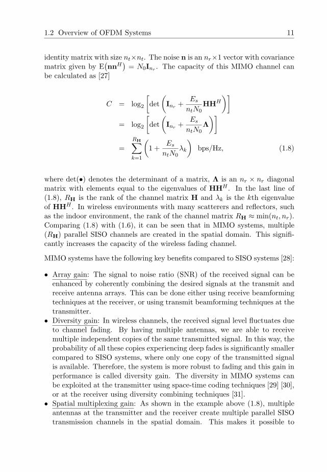
where det(•) denotes the determinant of a matrix, Λ is an nr × nr diagonalmatrix with elements equal to the eigenvalues of HHH . In the last line of(1.8), RH is the rank of the channel matrix H and λk is the kth eigenvalueof HHH . In wireless environments with many scatterers and reflectors, suchas the indoor environment, the rank of the channel matrix RH ≈ min(nt, nr).Comparing (1.8) with (1.6), it can be seen that in MIMO systems, multiple(RH) parallel SISO channels are created in the spatial domain. This signifi-cantly increases the capacity of the wireless fading channel.
MIMO systems have the following key benefits compared to SISO systems [28]:
• Array gain: The signal to noise ratio (SNR) of the received signal can beenhanced by coherently combining the desired signals at the transmit andreceive antenna arrays. This can be done either using receive beamformingtechniques at the receiver, or using transmit beamforming techniques at thetransmitter.
• Diversity gain: In wireless channels, the received signal level fluctuates dueto channel fading. By having multiple antennas, we are able to receivemultiple independent copies of the same transmitted signal. In this way, theprobability of all these copies experiencing deep fades is significantly smallercompared to SISO systems, where only one copy of the transmitted signalis available. Therefore, the system is more robust to fading and this gain inperformance is called diversity gain. The diversity in MIMO systems canbe exploited at the transmitter using space-time coding techniques [29] [30],or at the receiver using diversity combining techniques [31].
• Spatial multiplexing gain: As shown in the example above (1.8), multipleantennas at the transmitter and the receiver create multiple parallel SISOtransmission channels in the spatial domain. This makes it possible to
12 Chapter 1. Introduction
multiplex different data streams on different transmit antennas and achievea higher data rate using the same bandwidth.
• Interference mitigation: In a multi-user environment, interference from otherusers using the same frequency band can severely degrade the performanceof the desired user. This interference can be mitigated using signal process-ing techniques in the spatial dimension provided by MIMO systems. Forexample, using beamforming techniques, the receiver can create beam pat-terns with main lobes pointing to the desired user and with nulls pointingto the interfering users.
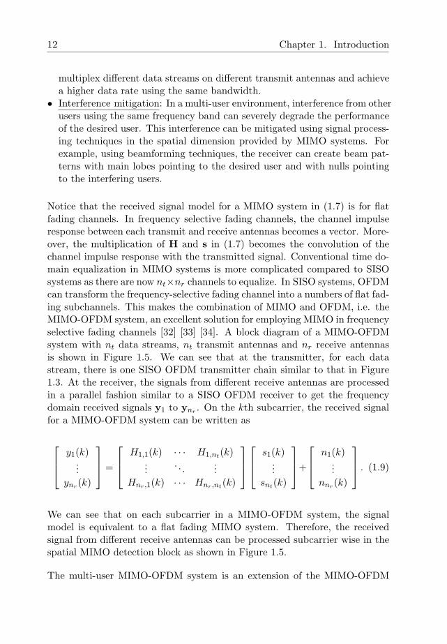
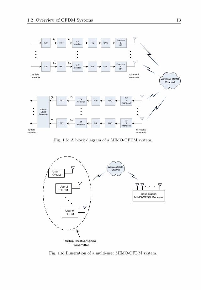
Notice that the received signal model for a MIMO system in (1.7) is for flatfading channels. In frequency selective fading channels, the channel impulseresponse between each transmit and receive antennas becomes a vector. More-over, the multiplication of H and s in (1.7) becomes the convolution of thechannel impulse response with the transmitted signal. Conventional time do-main equalization in MIMO systems is more complicated compared to SISOsystems as there are now nt×nr channels to equalize. In SISO systems, OFDMcan transform the frequency-selective fading channel into a numbers of flat fad-ing subchannels. This makes the combination of MIMO and OFDM, i.e. theMIMO-OFDM system, an excellent solution for employing MIMO in frequencyselective fading channels [32] [33] [34]. A block diagram of a MIMO-OFDMsystem with nt data streams, nt transmit antennas and nr receive antennasis shown in Figure 1.5. We can see that at the transmitter, for each datastream, there is one SISO OFDM transmitter chain similar to that in Figure1.3. At the receiver, the signals from different receive antennas are processedin a parallel fashion similar to a SISO OFDM receiver to get the frequencydomain received signals y1 to ynr . On the kth subcarrier, the received signalfor a MIMO-OFDM system can be written as
y1(k)...
ynr(k)
=
H1,1(k) · · · H1,nt(k)...
. . ....
Hnr,1(k) · · · Hnr,nt(k)
s1(k)...
snt(k)
+
n1(k)...
nnr(k)
. (1.9)
We can see that on each subcarrier in a MIMO-OFDM system, the signalmodel is equivalent to a flat fading MIMO system. Therefore, the receivedsignal from different receive antennas can be processed subcarrier wise in thespatial MIMO detection block as shown in Figure 1.5.
The multi-user MIMO-OFDM system is an extension of the MIMO-OFDM
1.2 Overview of OFDM Systems 13
S/P IFFTCP
InsertionP/S DAC
Front-end
&
RF
nt data
streams
nt transmit
antennasWireless MIMO
Channel
s1 x1
S/P IFFTCP
InsertionP/S DAC
Front-end
&
RF
snt xnt
FFTCP
RemovalS/P ADC
RF
&
Front-end
FFTCP
RemovalS/P ADC
RF
&
Front-end
Spatial
MIMO
Detection
nr receive
antennas
r1
rnr
nt data
streams
y1
ynr
Fig. 1.5: A block diagram of a MIMO-OFDM system.
User nt
OFDM
User 2
OFDM
User 1
OFDM
Base station
MIMO-OFDM Receiver
Virtual Multi-antenna
Transmitter
Wireless MIMO
Channel
Fig. 1.6: Illustration of a multi-user MIMO-OFDM system.
14 Chapter 1. Introduction
system to the multi-user context. An illustration of the multi-user MIMO-OFDM system is shown in Figure 1.6. Here multiple users, each with one ormore transmit antennas, transmit simultaneously using OFDM in the samefrequency band. For clearness of illustration, in Figure 1.6, we only illustratethe case where each user has one transmit antenna. The receiver is a basestation with multiple receive antennas. It uses MIMO-OFDM spatial process-ing techniques to separate the signals from different users. If we view thesignals from different users as signals from different transmit antennas of avirtual multi-antenna transmitter, then the whole system can be viewed asan MIMO-OFDM system. This system is also known as the virtual MIMO-OFDM system [35].
1.3 Effects of Frequency Synchronization Errors in
OFDM Systems
In the previous section, we presented an overview of OFDM and MIMO-OFDMsystems. We highlighted the advantages of OFDM and MIMO-OFDM and alsomentioned that sensitivity to frequency synchronization errors in the form ofcarrier frequency offset (CFO), is a key disadvantage of OFDM systems. Inthis section, we present a more detailed study on the effects of CFO on the per-formance of OFDM systems. As the name suggests, CFO is an offset betweenthe carrier frequency of the transmitted signal and the carrier frequency usedat the receiver for demodulation. In wireless communications, CFO comesmainly from two sources:
• The mismatch between oscillating frequencies of the transmitter and thereceiver local oscillators (LO);
• The Doppler effect of the channel due to relative movement between thetransmitter and the receiver.
In this thesis, we focus on the CFO caused by the mismatch between thetransmitter and receiver local oscillators. At the receiver, the effect of CFO ismitigated through frequency synchronization. Figure 1.7 shows an OFDM re-ceiver with frequency synchronization implemented in both the analog and thedigital domains. The received signal from the receive antenna is first passed tothe receiver front-end. Here, to ensure that the local oscillator at the receiver
1.3 Effects of Frequency Synchronization Errors in OFDM Systems 15
Digital CFO
Estimation
-CP
&
FFTdetector ADC
ry
Receiver
Front-end
Analog
Coarse
Freq Sync
Residual
CFO
tracking
Receive
Antenna
(2 / )j n Ne πε θ+
Crystal Oscillator
Frequency
Synthesizer
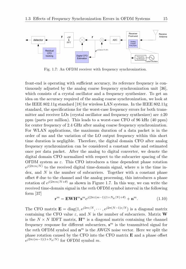
Fig. 1.7: An OFDM receiver with frequency synchronization.
front-end is operating with sufficient accuracy, its reference frequency is con-tinuously adjusted by the analog coarse frequency synchronization unit [36],which consists of a crystal oscillator and a frequency synthesizer. To get anidea on the accuracy required of the analog coarse synchronization, we look atthe IEEE 802.11g standard [18] for wireless LAN systems. In the IEEE 802.11gstandard, the specifications for the worst-case frequency errors for both trans-mitter and receiver LOs (crystal oscillator and frequency synthesizer) are ±20ppm (parts per million). This leads to a worst-case CFO of 96 kHz (40 ppm)for center frequency of 2.4 GHz after analog coarse frequency synchronization.For WLAN applications, the maximum duration of a data packet is in theorder of ms and the variation of the LO output frequency within this shorttime duration is negligible. Therefore, the digital domain CFO after analogfrequency synchronization can be considered a constant value and estimatedonce per data packet. After the analog to digital converter, we denote thedigital domain CFO normalized with respect to the subcarrier spacing of theOFDM system as ε. This CFO introduces a time dependent phase rotationej(2πεn/N) to the received digital time-domain signal, where n is the time in-dex, and N is the number of subcarriers. Together with a constant phaseoffset θ due to the channel and the analog processing, this introduces a phaserotation of ej(2πεn/N+θ) as shown in Figure 1.7. In this way, we can write thereceived time-domain signal in the mth OFDM symbol interval in the followingform [37]
rm = EWHmsmej(2πε(m−1)(1+Ng/N)+θ) + nm. (1.10)
The CFO matrix E = diag(1, ej2πε/N , · · · , ej2π(N−1)ε/N ) is a diagonal matrixcontaining the CFO value ε, and N is the number of subcarriers. Matrix Wis the N ×N IDFT matrix, Hm is a diagonal matrix containing the channelfrequency response for different subcarriers, sm is the transmitted signal forthe mth OFDM symbol and nm is the AWGN noise vector. Here we split thephase rotation caused by the CFO into the CFO matrix E and a phase offsetej2πε(m−1)(1+Ng/N) for OFDM symbol m.
16 Chapter 1. Introduction
Notice from (1.10) that the effects of the CFO ε and the constant phase offsetθ are represented in the following three terms:
1. a constant phase offset ejθ,2. a CFO matrix E,3. a CFO and OFDM symbol index (m) dependent phase offset
ej(2πε(m−1)(1+Ng/N)).
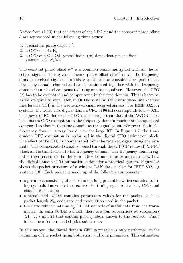
The constant phase offset ejθ is a common scalar multiplied with all the re-ceived signals. This gives the same phase offset of ejθ on all the frequencydomain received signals. In this way, it can be considered as part of thefrequency domain channel and can be estimated together with the frequencydomain channel and compensated using one-tap equalizers. However, the CFO(ε) has to be estimated and compensated in the time domain. This is because,as we are going to show later, in OFDM systems, CFO introduces inter-carrierinterference (ICI) in the frequency-domain received signals. For IEEE 802.11gsystems, the worst-case digital domain CFO of 96 kHz corresponds to ε = 0.31.The power of ICI due to this CFO is much larger than that of the AWGN noise.This makes CFO estimation in the frequency domain much more complicatedcompared to that in the time domain as the signal to interference ratio in thefrequency domain is very low due to the large ICI. In Figure 1.7, the time-domain CFO estimation is performed in the digital CFO estimation block.The effect of the CFO is compensated from the received signal using the esti-mate. The compensated signal is passed through the -CP(CP removal) & FFTblock and is transformed to the frequency domain. The frequency-domain sig-nal is then passed to the detector. Now let us use an example to show howthe digital domain CFO estimation is done for a practical system. Figure 1.8shows the packet structure of a wireless LAN data packet for IEEE 802.11gsystems [18]. Each packet is made up of the following components:
• a preamble, consisting of a short and a long preamble, which contains train-ing symbols known to the receiver for timing synchronization, CFO andchannel estimation;
• a signal field, which contains parameters values for the packet, such aspacket length Np, code rate and modulation used in the packet;
• the data: which contains Np OFDM symbols of useful data from the trans-mitter. In each OFDM symbol, there are four subcarriers at subcarriers-21, -7, 7 and 21 that contain pilot symbols known to the receiver. Thesefour subcarriers are called pilot subcarriers.
In this system, the digital domain CFO estimation is only performed at thebeginning of the packet using both short and long preambles. This estimation
1.3 Effects of Frequency Synchronization Errors in OFDM Systems 17
Signal
Field
OFDM
Symbol 1
OFDM
Symbol 2
OFDM
Symbol Np
Preamble Data: Np OFDM Symbols
Short Preamble Long Preamble
-21 -7 7 21
Subcarrier Number
Pilot 3Pilot 2Pilot 1 Pilot 4
Fig. 1.8: The packet structure of a IEEE 802.11g data packet.
must achieve sufficient accuracy such that ICI due to the residual CFO ∆ε,i.e. the difference between the actual ε and its estimate, is significantly smallerthan the AWGN noise. The constant phase offset ejθ is estimated as part of thechannel using the long preamble. Although the ICI due to ∆ε is insignificant,the residual CFO still causes a OFDM symbol index (m) dependent phaseoffset ej(2π∆ε(m−1)(1+Ng/N)). Different from the constant phase offset ejθ, thisphase offset cannot be estimated using channel estimation, because the channelis only estimated at the beginning of the packet using the long preamble, andcan become significant when the number of OFDM symbols in a packet is large.This phase offset is estimated and compensated in the frequency domain inthe residual CFO tracking block as shown in Figure 1.7 using the four pilotsubcarriers in each OFDM symbol. Notice that this phase offset estimation isdone after the initial CFO estimation and compensation using the preambles,because without the initial CFO estimation and compensation, the ICI fromthe CFO will become too large for the phase offset estimation to work properly.As this block is only necessary for packet-based OFDM systems, where CFOand channel estimations are performed at the beginning of the packet, we usedotted lines in Figure 1.7 to indicate that it is optional. The research work inthis thesis concerns the time domain estimation of the CFO ε.
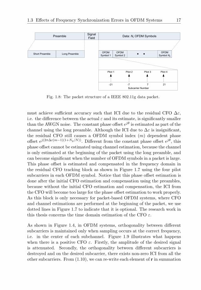
As shown in Figure 1.4, in OFDM systems, orthogonality between differentsubcarriers is maintained only when sampling occurs at the correct frequency,i.e. in the center of each subchannel. Figure 1.9 illustrates what happenswhen there is a positive CFO ε. Firstly, the amplitude of the desired signalis attenuated. Secondly, the orthogonality between different subcarriers isdestroyed and on the desired subcarrier, there exists non-zero ICI from all theother subcarriers. From (1.10), we can re-write each element of r in summation
18 Chapter 1. Introduction
0 2 4 6 8 10 12 14 160
0.2
0.4
0.6
0.8
1
1.2
Subcarrier (k)
Am
plitu
de
AmplitudeAttenuation
Non−zero ICI
ε
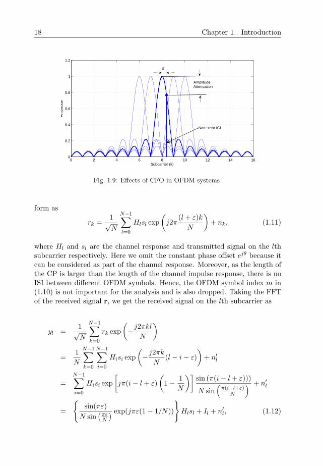
Fig. 1.9: Effects of CFO in OFDM systems
form as
rk =1√N
N−1∑
l=0
Hlsl exp(
j2π(l + ε)k
N
)+ nk, (1.11)
where Hl and sl are the channel response and transmitted signal on the lthsubcarrier respectively. Here we omit the constant phase offset ejθ because itcan be considered as part of the channel response. Moreover, as the length ofthe CP is larger than the length of the channel impulse response, there is noISI between different OFDM symbols. Hence, the OFDM symbol index m in(1.10) is not important for the analysis and is also dropped. Taking the FFTof the received signal r, we get the received signal on the lth subcarrier as
yl =1√N
N−1∑
k=0
rk exp(−j2πkl
N
)
=1N
N−1∑
k=0
N−1∑
i=0
Hisi exp(−j2πk
N(l − i− ε)
)+ n′l
=N−1∑
i=0
Hisi exp[jπ(i− l + ε)
(1− 1
N
)]sin (π(i− l + ε)))
N sin(
π(i−l+ε)N
) + n′l
=
sin(πε)
N sin(
πεN
) exp(jπε(1− 1/N))
Hlsl + Il + n′l, (1.12)
1.3 Effects of Frequency Synchronization Errors in OFDM Systems 19
0 0.1 0.2 0.3 0.4 0.5−5
0
5
10
15
20
25
Frequency Offset (ε)
SIN
R (
dB)
SNR=5dBSNR=10dBSNR=15dBSNR=25dB
Fig. 1.10: SINR of the received signal in OFDM systems for different CFO values.
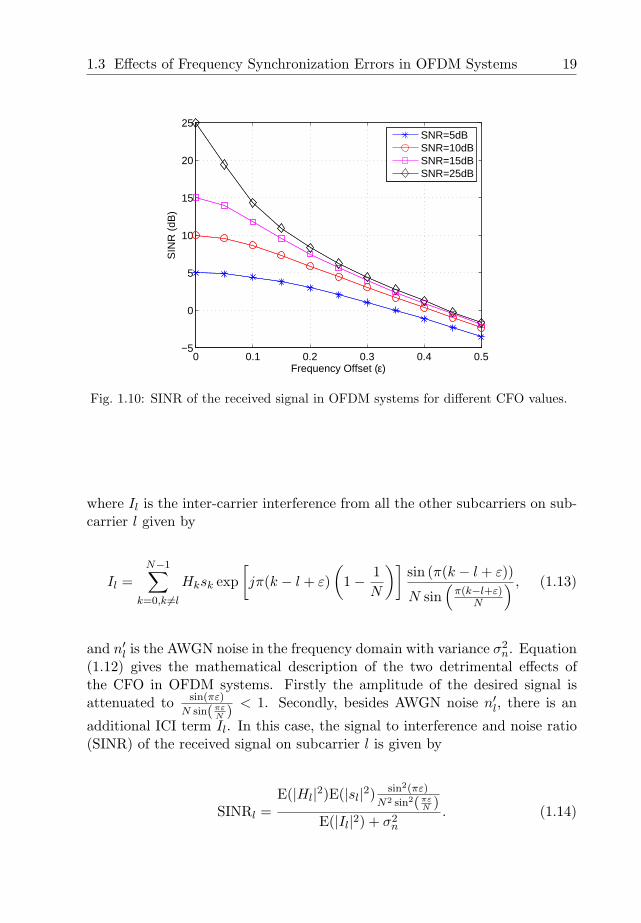
where Il is the inter-carrier interference from all the other subcarriers on sub-carrier l given by
Il =N−1∑
k=0,k 6=l
Hksk exp[jπ(k − l + ε)
(1− 1
N
)]sin (π(k − l + ε))
N sin(
π(k−l+ε)N
) , (1.13)
and n′l is the AWGN noise in the frequency domain with variance σ2n. Equation
(1.12) gives the mathematical description of the two detrimental effects ofthe CFO in OFDM systems. Firstly the amplitude of the desired signal isattenuated to sin(πε)
N sin(πεN ) < 1. Secondly, besides AWGN noise n′l, there is an
additional ICI term Il. In this case, the signal to interference and noise ratio(SINR) of the received signal on subcarrier l is given by
SINRl =E(|Hl|2)E(|sl|2) sin2(πε)
N2 sin2(πεN )
E(|Il|2) + σ2n
. (1.14)
20 Chapter 1. Introduction
In Figure 1.10, we plot the SINR given in (1.14) for an OFDM system with64 subcarriers for different CFO values and for 4 signal to AWGN noise ra-tios (E[|H|2|s|2]/σ2
n ) of 5, 10, 15 and 25 dB. From the figure, we can seethat the SINR degrades significantly as the CFO value increases. As the ICIpower is independent of the AWGN noise power, the ICI causes more degra-dation in high SNR cases compared to low SNR cases. From Figure 1.10,the worst-case CFO of ε = 0.31 in IEEE 802.11g WLAN systems causes adegradation of about 21 dB for SNR of 25 dB. In the same vein, CFO alsocauses significant performance degradation for MIMO-OFDM and multi-userMIMO-OFDM systems. Therefore, to guarantee good performance of OFDMsystems, CFO must be accurately estimated and compensated.
1.4 Status and Challenges in CFO estimation for
OFDM systems
In this section, we present a brief literature review on CFO estimation algo-rithms for OFDM systems. We also identify challenges in the CFO estimationfor SISO, MIMO and multi-user MIMO OFDM systems and motivate theresearch work carried out in this thesis.
1.4.1 CFO estimation for SISO-OFDM systems
The CFO estimation algorithms for SISO-OFDM systems can be broadly di-vided into two categories:
1. Training-based CFO estimation algorithms;2. Blind CFO estimation algorithms.
1.4.1.1 Training based CFO estimation algorithms
In training-based CFO estimation algorithms, specially designed training sig-nals (including preambles and/or pilot subcarriers) known to the receiver areinserted into the data symbols to assist the receiver in estimating the CFO.
1.4 Status and Challenges in CFO estimation for OFDM systems 21
Two well-known training-based CFO estimation algorithms for SISO-OFDMsystems were proposed by P. Moose [38] and by T.M. Schmidl & D.C. Cox [39].
In Moose’s algorithm, two repeated OFDM symbols are transmitted as train-ing symbols. As the second OFDM symbol is identical to the first one, thelast Ng samples of the first OFDM symbol have the same effect as the cyclicprefix for the second OFDM symbol. Hence, it is not necessary to append aCP to the second OFDM symbol. The assumption in this algorithm is thatthe starting point of an OFDM symbol is known. In this case, using similarnotations as in (1.10), the time domain received signals in these two OFDMsymbol intervals can be written as
r =[
EWHsej2πεEWHs
]+ n, (1.15)
where r is a 2N × 1 vector containing received signal for two OFDM symbols.Here we assume a slowly time-varying channel such that the channel withinthe two OFDM symbol intervals can be considered the same. Taking the FFTof the received signals, we get the frequency-domain signals in the two OFDMsymbol intervals given by
y =[
WHEWHsej2πεWHEWHs
]+ n′, (1.16)
where n′ is the frequency domain noise vector, which has the same statisticalproperties as n. In the noiseless condition, the difference between the first andthe second N elements of y is a constant phase shift of ej2πε due to the CFO.It is shown in [38] that the maximum likelihood (ML) estimate of the CFO εis given by
ε =12π
tan−1
∑N−1l=0 =[yl+Ny∗l ]∑N−1l=0 <[yl+Ny∗l ]
, (1.17)
where =(•) and <(•) denote the imaginary and the real parts of a complexnumber respectively and superscript ∗ denotes complex conjugation. It isshown in [38] that this estimate is conditionally unbiased for small CFO values.
22 Chapter 1. Introduction
The mean square error (MSE) of this estimator is given by
MSE(ε) =1
(2π)2Nγ, (1.18)
where
γ =tr
(HHH
)
N
σ2s
σ2n
is the SNR of the received signal. Here we use tr(•) to denote the trace ofa matrix, and σ2
s and σ2n are the power of the transmitted signal and noise
respectively. The acquisition range of this algorithm is limited in ±0.5 subcar-rier spacing. This is smaller than the worst-case CFO of 0.64 in IEEE 802.11awireless LAN systems operating in the 5 GHz band. It is suggested in [38]that the acquisition range can be increased by using shorter repeated frequencydomain training symbols. Decreasing the length of the training symbol by afactor of n will increase the acquisition range n times. On the other hand, from(1.18), we can see that reducing the length of training symbol degrades theMSE of the CFO estimation. The length of the training symbol also needs tobe kept longer than the channel delay spread so as not to cause any distortionwhen estimating the CFO.
One limitation of Moose’s algorithm is that it requires knowledge of the start-ing point of an OFDM symbol. In [39], Schmidl & Cox proposed an algo-rithm that can estimate timing and frequency offset using the same time-domain training sequence. In their method, the time-domain OFDM sym-bol used for training consists of two identical halves, i.e. xk = xk+N/2 fork = 0, · · · , N/2−1. At the receiver, it can be easily shown that rk+N/2 = ejπεrk
for k = 0, · · · , N/2− 1. Here k = 0 corresponds to the index of the first time-domain sample after the CP. Hence, the received signal also consists of twoidentical halves, except for a phase difference ejπε that is caused by the CFO.To determine the start of the OFDM symbol, in [39], a timing metric is cal-culated as
Mk =
∣∣∣∑N/2−1m=0 r∗k+mrk+m+N/2
∣∣∣2
∑N/2−1m=0
∣∣rk+m+N/2
∣∣2 . (1.19)
We can see that the numerator of M(k) in (1.19) is an autocorrelation functionof the received signal in a window of size N/2, while the denominator in (1.19)is a normalization constant equal to the power of the second-half of the training
1.4 Status and Challenges in CFO estimation for OFDM systems 23
−400 −300 −200 −100 0 100 200 3000
0.1
0.2
0.3
0.4
0.5
0.6
0.7
0.8
0.9
1
Timing Offset
Tim
ing
Met
ric
Fig. 1.11: An example of timing metric using the autocorrelation method (AWGNChannel SNR=20dB).
symbol.
Figure 1.11 shows an example of the timing metric Mk for an OFDM systemwith 512 subcarriers and cyclic prefix equal to 64. The channel is an AWGNchannel with SNR of 20 dB and the CFO ε = 0.6. Here we put the start ofthe OFDM symbol as the 0 timing point. We can see that the timing metricfunction reaches a plateau of length equal to the length of the cyclic prefix.For multi-path fading channel, the length of the plateau is equal to the lengthof the cyclic prefix minus the length of the channel impulse response. Thestarting point of the OFDM symbol can be taken at any point on the plateauand there will be no inter-symbol interference (ISI) [39]. Once the timing pointk is determined, it is shown in [39] that the ML estimate of the CFO can beobtained as
ε =1π
∠
N/2−1∑
m=0
r∗k+mrk+m+N/2
=1π
tan−1
=
(∑N/2−1m=0 r∗k+mrk+m+N/2
)
<(∑N/2−1
m=0 r∗k+mrk+m+N/2
) , (1.20)
24 Chapter 1. Introduction
where ∠(•) denotes the angle of a complex number. The CFO estimator in(1.20) has an acquisition range of ±1 subcarrier spacing and the MSE of theCFO estimation is given by [39]
MSE(ε) =2
π2Nγ, (1.21)
which has a similar expression as the frequency domain method in (1.18).
Both methods in [38] and [39] use periodic training sequences in either thefrequency or the time domain to estimate the CFO in OFDM systems. Inboth methods, the ML CFO estimate can be obtained using simple correlationoperations as shown in (1.17) and (1.20). Compared to the frequency domainmethod in [38], the time domain method in [39] has two advantages. Firstly,timing synchronization can be obtained using the same training sequence.Secondly, frequency synchronization is performed in the time domain, thusit saves the complexity of FFT operations required in the frequency domainmethods. As a result, time-domain periodic training sequences have beenadopted in various wireless standards as the training sequence for timing andCFO estimation [17] [18] [5]. In [40], the authors extended the CFO estimationusing periodic sequences to the case where the number of periods is largerthan 2. A more practical treatment on CFO and timing estimation in OFDMsystems was given in [41]. The acquisition range of CFO values and methodto resolve the ambiguity in CFO estimation were addressed in [42]. In [43]and [44], the CFO and timing estimation algorithms were studied specificallyin the context of IEEE 802.11 training sequences. The Cramer-Rao bounds(CRB) for CFO estimation using a general and a periodic training sequencein frequency selective fading channels were derived in [45].
In summary, the use of periodic training sequences for CFO estimation inSISO-OFDM systems has been extensively studied in both theoretical andpractical aspects. Moreover, the computational complexity required for CFOestimation in SISO-OFDM systems is already very small. Therefore, in thisthesis, we will not further study the training-based CFO estimation in SISO-OFDM systems. However, training-based CFO estimation algorithms havesome limitations. The training sequence used for CFO estimation is an ex-tra overhead for transmission and it reduces the effective data throughput ofthe system. For a typical application like IEEE 802.11a/g WLAN, the totaloverhead used for CFO estimation and residual CFO tracking, including boththe short preamble and the pilots, is about 10% of the total data throughput.
1.4 Status and Challenges in CFO estimation for OFDM systems 25
The WLAN system is designed for low mobility applications, in which theCFO can be assumed to be constant within a packet. In the case of mobilesystems, the CFO becomes time varying due to the Doppler effect of the chan-nel [46]. This requires more frequent transmission of training sequences, whichfurther reduces the data throughput. To avoid this problem, in this thesis, westudy another class of CFO estimation algorithms, namely blind algorithms,for SISO-OFDM systems. Blind algorithms do not require training sequencesand hence have no training overhead. The disadvantage is that their compu-tational complexity is normally higher than that of training-based algorithms.A detailed overview on blind CFO estimation algorithms for SISO-OFDMsystems is given in Section 1.4.1.2.
For MIMO-OFDM and multi-user MIMO-OFDM systems, the computationalcomplexity for blind algorithms becomes too high for practical implementa-tions. Therefore, in Chapter 5 and Chapter 6, we will come back to training-based algorithms. We will study low complexity CFO estimation algorithmsfor MIMO-OFDM and multi-user MIMO-OFDM systems using periodic train-ing sequences.
1.4.1.2 Blind CFO estimation algorithms
Blind CFO estimation algorithms are a class of algorithms where the CFO isestimated using the statistical properties of the received signal only, withoutexplicit knowledge of the transmitted signal. Therefore, it does not requiretraining sequences. In SISO-OFDM systems, blind CFO estimation algorithmsusually make use of some special properties of OFDM symbols such as thecyclic prefix in the time domain and guard null subcarriers in the frequencydomain.
In [47], the authors proposed a CFO estimation algorithm making use of thetime-domain cyclic prefix in OFDM systems. For an AWGN channel, thereceived time-domain OFDM signal has the following property
Er∗krk+N = σ2s exp(j2πε) + σ2
n, (1.22)
if k is in the part of the OFDM symbol that corresponds to the cyclic prefix.Based on this property, the authors showed that a maximum-likelihood CFO
26 Chapter 1. Introduction
estimator is given by
ε =12π
∠
t+Ng−1∑
k=t
r∗krk+N
, (1.23)
where t is the start of the cyclic prefix portion of the received signal. From(1.23), we can see that CFO estimation only requires the computation of theautocorrelation of the received signal. Therefore, the computational complex-ity is low. However, there are a few drawbacks of this method. Firstly, if thechannel is dispersive, the number of terms in (1.23) is equal to the differenceof CP length and the length of the channel impulse response. In this case,the MSE of the CFO estimation is degraded compared to that in flat fadingchannels. Secondly the acquisition range of this method is limited to ±0.5subcarrier spacing.
Another popular blind CFO estimation method was proposed by Liu andTureli in [37]. This method makes use of the frequency-domain characteris-tics of OFDM systems. Figure 1.12 shows the spectrum of a practical OFDMsystem with N subcarriers. In this system, there are d1 and d2 subcarriersat two ends of the allocated spectrum that are left empty and used as guardbands to avoid aliasing to the adjacent channels [17]. We will refer to the non-data-carrying subcarriers as null subcarriers and we call the data-carryingsubcarriers data subcarriers. In the absence of noise and ICI, the receivedsignal on the null subcarriers should be 0. Based on this observation, Liuand Tureli proposed a blind CFO estimation algorithm based on the mini-mization of the received signal power on null subcarriers [37]. It was shownin [48] that this CFO estimation method is optimal in the ML sense. Becauseit makes use of the frequency-domain characteristics of OFDM systems, itsperformance is not affected by the length of the channel impulse response.Moreover, compared to the method in [47], it is more robust against timingerrors. A disadvantage of the algorithm is its computational complexity. Thisis because the cost function in the minimization problem in [37] is a polyno-mial with the complex variable of order 2(N − 1). For a typical application,like wireless LAN, N = 64 [17]. Hence, the order of the cost function becomes126, and the computational complexity required to find the minimum is veryhigh. Therefore, it is important to find methods to reduce the computationalcomplexity of the blind algorithm in [37] to make it implementable in practice.Moreover, it is also important that the reduction in complexity does not leadto big performance degradations. Finding such a solution is a technical chal-
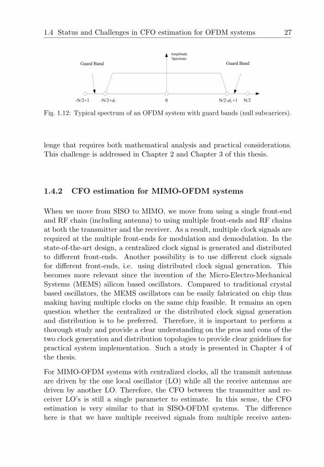
1.4 Status and Challenges in CFO estimation for OFDM systems 27
-N/2+1 0 N/2-N/2+d1 N/2-d2+1
Guard Band Guard Band
Amplitude
Spectrum
Fig. 1.12: Typical spectrum of an OFDM system with guard bands (null subcarriers).
lenge that requires both mathematical analysis and practical considerations.This challenge is addressed in Chapter 2 and Chapter 3 of this thesis.
1.4.2 CFO estimation for MIMO-OFDM systems
When we move from SISO to MIMO, we move from using a single front-endand RF chain (including antenna) to using multiple front-ends and RF chainsat both the transmitter and the receiver. As a result, multiple clock signals arerequired at the multiple front-ends for modulation and demodulation. In thestate-of-the-art design, a centralized clock signal is generated and distributedto different front-ends. Another possibility is to use different clock signalsfor different front-ends, i.e. using distributed clock signal generation. Thisbecomes more relevant since the invention of the Micro-Electro-MechanicalSystems (MEMS) silicon based oscillators. Compared to traditional crystalbased oscillators, the MEMS oscillators can be easily fabricated on chip thusmaking having multiple clocks on the same chip feasible. It remains an openquestion whether the centralized or the distributed clock signal generationand distribution is to be preferred. Therefore, it is important to perform athorough study and provide a clear understanding on the pros and cons of thetwo clock generation and distribution topologies to provide clear guidelines forpractical system implementation. Such a study is presented in Chapter 4 ofthe thesis.
For MIMO-OFDM systems with centralized clocks, all the transmit antennasare driven by the one local oscillator (LO) while all the receive antennas aredriven by another LO. Therefore, the CFO between the transmitter and re-ceiver LO’s is still a single parameter to estimate. In this sense, the CFOestimation is very similar to that in SISO-OFDM systems. The differencehere is that we have multiple received signals from multiple receive anten-
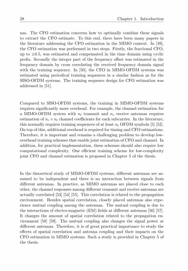
28 Chapter 1. Introduction
nas. The CFO estimation concerns how to optimally combine these signalsto extract the CFO estimate. To this end, there have been many papers inthe literature addressing the CFO estimation in the MIMO context. In [49],the CFO estimation was performed in two steps. Firstly, the fractional CFO,up to ±0.5, was estimated and compensated in the time domain using cyclicprefix. Secondly the integer part of the frequency offset was estimated in thefrequency domain by cross correlating the received frequency domain signalwith the training sequence. In [50], the CFO in MIMO-OFDM systems wasestimated using periodical training sequences in a similar fashion as for theSISO-OFDM systems. The training sequence design for CFO estimation wasaddressed in [51].
Compared to SISO-OFDM systems, the training in MIMO-OFDM systemsrequires significantly more overhead. For example, the channel estimation fora MIMO-OFDM system with nt transmit and nr receive antennas requiresestimation of nr×nt channel coefficients for each subcarrier. In the literature,this normally requires training sequences of at least nt OFDM symbols [5] [52].On top of this, additional overhead is required for timing and CFO estimations.Therefore, it is important and remains a challenging problem to develop low-overhead training schemes that enable joint estimation of CFO and channel. Inaddition, for practical implementation, these schemes should also require lowcomputational complexity. One efficient training scheme for low-complexityjoint CFO and channel estimation is proposed in Chapter 5 of the thesis.
In the theoretical study of MIMO-OFDM systems, different antennas are as-sumed to be independent and there is no interaction between signals fromdifferent antennas. In practice, as MIMO antennas are placed close to eachother, the channel responses among different transmit and receive antennas areactually correlated [53] [54] [55]. This correlation is related to the propagationenvironment. Besides spatial correlation, closely placed antennas also expe-rience mutual coupling among the antennas. The mutual coupling is due tothe interactions of electro-magnetic (EM) fields at different antennas [56] [57].It changes the amount of spatial correlation related to the propagation en-vironment [58] [59]. The mutual coupling also changes the signal power atdifferent antennas. Therefore, it is of great practical importance to study theeffects of spatial correlation and antenna coupling and their impacts on theCFO estimation in MIMO systems. Such a study is provided in Chapter 5 ofthe thesis.
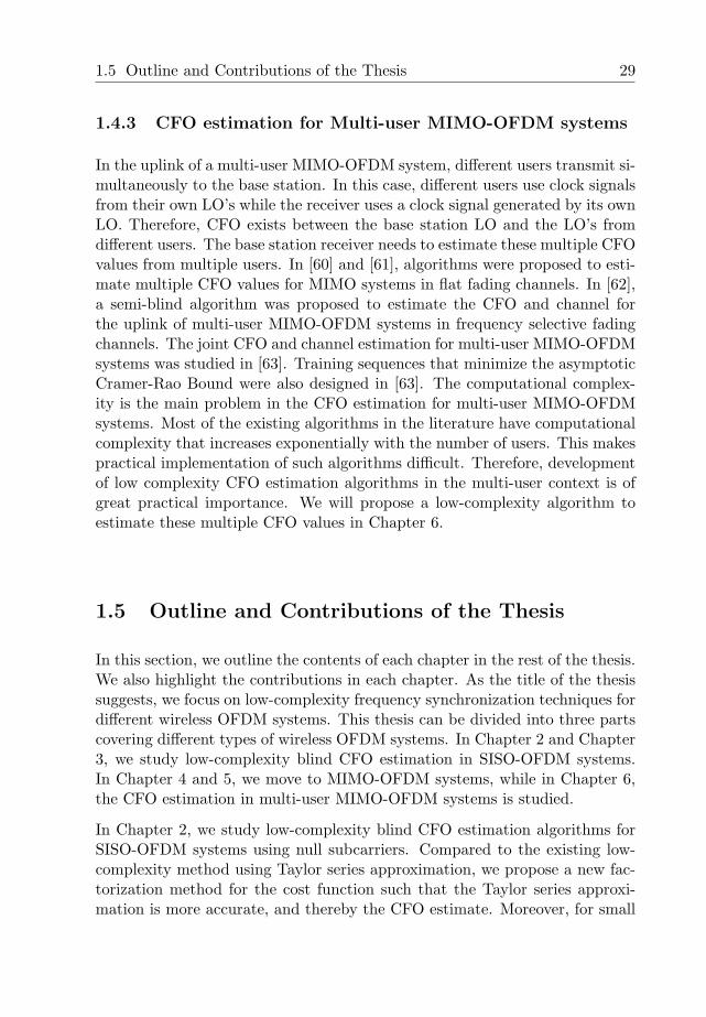
1.5 Outline and Contributions of the Thesis 29
1.4.3 CFO estimation for Multi-user MIMO-OFDM systems
In the uplink of a multi-user MIMO-OFDM system, different users transmit si-multaneously to the base station. In this case, different users use clock signalsfrom their own LO’s while the receiver uses a clock signal generated by its ownLO. Therefore, CFO exists between the base station LO and the LO’s fromdifferent users. The base station receiver needs to estimate these multiple CFOvalues from multiple users. In [60] and [61], algorithms were proposed to esti-mate multiple CFO values for MIMO systems in flat fading channels. In [62],a semi-blind algorithm was proposed to estimate the CFO and channel forthe uplink of multi-user MIMO-OFDM systems in frequency selective fadingchannels. The joint CFO and channel estimation for multi-user MIMO-OFDMsystems was studied in [63]. Training sequences that minimize the asymptoticCramer-Rao Bound were also designed in [63]. The computational complex-ity is the main problem in the CFO estimation for multi-user MIMO-OFDMsystems. Most of the existing algorithms in the literature have computationalcomplexity that increases exponentially with the number of users. This makespractical implementation of such algorithms difficult. Therefore, developmentof low complexity CFO estimation algorithms in the multi-user context is ofgreat practical importance. We will propose a low-complexity algorithm toestimate these multiple CFO values in Chapter 6.
1.5 Outline and Contributions of the Thesis
In this section, we outline the contents of each chapter in the rest of the thesis.We also highlight the contributions in each chapter. As the title of the thesissuggests, we focus on low-complexity frequency synchronization techniques fordifferent wireless OFDM systems. This thesis can be divided into three partscovering different types of wireless OFDM systems. In Chapter 2 and Chapter3, we study low-complexity blind CFO estimation in SISO-OFDM systems.In Chapter 4 and 5, we move to MIMO-OFDM systems, while in Chapter 6,the CFO estimation in multi-user MIMO-OFDM systems is studied.
In Chapter 2, we study low-complexity blind CFO estimation algorithms forSISO-OFDM systems using null subcarriers. Compared to the existing low-complexity method using Taylor series approximation, we propose a new fac-torization method for the cost function such that the Taylor series approxi-mation is more accurate, and thereby the CFO estimate. Moreover, for small
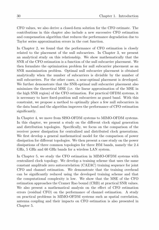
30 Chapter 1. Introduction
CFO values, we also derive a closed-form solution for the CFO estimate. Thecontributions in this chapter also include a new successive CFO estimationand compensation algorithm that reduces the performance degradation due toTaylor series approximation errors in the cost function.
In Chapter 2, we found that the performance of CFO estimation is closelyrelated to the placement of the null subcarriers. In Chapter 3, we presentan analytical study on this relationship. We show mathematically that theSNR of the CFO estimation is a function of the null subcarrier placement. Wethen formulate the optimization problem for null subcarrier placement as anSNR maximization problem. Optimal null subcarrier placement is obtainedanalytically when the number of subcarriers is divisible by the number ofnull subcarriers. For the other cases, a near-optimal placement is developed.We further demonstrate that the SNR-optimal null subcarrier placement alsominimizes the theoretical MSE (i.e. the linear approximation of the MSE inthe high SNR region) of the CFO estimation. For practical OFDM systems, itis necessary to have fixed-position null subcarriers as guard band. With thisconstraint, we propose a method to optimally place a few null subcarriers inthe data band and the algorithm improves the performance of CFO estimationsignificantly.
In Chapter 4, we move from SISO-OFDM systems to MIMO-OFDM systems.In this chapter, we present a study on the different clock signal generationand distribution topologies. Specifically, we focus on the comparison of thereceiver power dissipation for centralized and distributed clock generations.We first develop a general mathematical model for the comparison of powerdissipation for different topologies. We then present a case study on the powerdissipations of three common topologies for three ISM bands, namely the 2.4GHz, 5 GHz and 60 GHz bands for a wireless LAN system.
In Chapter 5, we study the CFO estimation in MIMO-OFDM systems withcentralized clock topology. We develop a training scheme that uses the sameconstant amplitude zero autocorrelation (CAZAC) training sequence for jointCFO and channel estimation. We demonstrate that the training overheadcan be significantly reduced using the developed training scheme and thatthe computational complexity is low. We show that the MSE of the CFOestimation approaches the Cramer Rao bound (CRB) at practical SNR values.We also present a mathematical analysis on the effect of CFO estimationerrors (residual CFO) on the performance of channel estimation. A studyon practical problems in MIMO-OFDM systems such as spatial correlation,antenna coupling and their impacts on CFO estimation is also presented inChapter 5.
1.6 List of Publications by the Author 31
The CFO estimation for multi-user MIMO-OFDM systems is studied in Chap-ter 6. We first derive the ML CFO estimator and show that the computationalcomplexity grows exponentially with the number of users. To reduce this com-plexity, we develop a sub-optimal CFO estimation algorithm using constantamplitude zero autocorrelation (CAZAC) sequences, the complexity of whichgrows only linearly with the number of users. The multiple CFO values in theuplink cause interference in the CFO estimation of different users using the pro-posed low-complexity algorithm.. To mitigate this interference, we propose amethod to find the CAZAC sequence that maximize the signal-to-interferenceratio for different classes of CAZAC sequences.
The concluding remarks of this thesis in given in Chapter 7 together withsuggestions for possible future work.
1.6 List of Publications by the Author
The research work carried out in this thesis has resulted in the following pub-lications.
1.6.1 Journals
1. S. Attallah, Y. Wu, and J.W.M. Bergmans, “Low complexity blind esti-mation of residual carrier offset in OFDM-based wireless LAN systems”,IET Communications, vol. 1, no. 4, pp. 604-611, Aug. 2007.Chapter 2
2. Y. Wu, S. Attallah, and J.W.M. Bergmans, “On the optimality of the nullsubcarrier placement for blind carrier offset estimation in OFDM systems”,IEEE Trans. Veh. Technol., vol. 58, no. 4, pp. 2109-2115, May 2009.Chapter 3
3. Y. Wu, J.W.M. Bergmans, and S. Attallah, “Carrier frequency offset es-timation for multi-user MIMO OFDM uplink using CAZAC sequences:performance and sequence optimization”, submitted to IEEE Trans. Sig-nal Process. .Chapter 6
32 Chapter 1. Introduction
1.6.2 Conference Proceedings
1. Y. Wu, S. Attallah, and J.W.M. Bergmans, “Blind iterative carrier offsetestimation for OFDM systems”, in Proc. IEEE International Symposiumon Signal Processing and its Applications, vol. 1, pp. 123-126, Aug. 2005.Chapter 2
2. Y. Wu, S. Attallah, and J.W.M. Bergmans, “On the SNR-optimal nullsubcarrier placement for blind carrier offset estimation in OFDM systems”,in Proc. IEEE Global Telecommunications Conference, Nov. 2006.Chapter 3
3. S. Attallah, Y. Wu, and J.W.M. Bergmans, “Low complexity blind residualcarrier offset estimation in OFDM-based wireless LAN systems”, in Proc.IEEE Wireless Communications and Networking Conference, pp. 1970-1975, Mar. 2007.Chapter 2
4. Y. Wu, S. Attallah, and J.W.M. Bergmans, “Efficient training sequencefor joint carrier frequency offset and channel estimation for MIMO-OFDMsystems”, in Proc. IEEE International Conference on Communications,pp. 2604-2609, Jun. 2007Chapter 5
5. Y. Wu, J.P. Linnartz, J.W.M. Bergmans, and S. Attallah, “Effects of an-tenna mutual coupling on the performance of MIMO systems”, in Proc.29th Symposium on Information Theory in the Benelux, pp. 207- 214,May 2008.Chapter 5
6. Y. Wu, S. Attallah, and J.W.M. Bergmans, “Carrier Frequency offset esti-mation for multi-user MIMO OFDM uplink using CAZAC sequences”, Ac-cepted IEEE Wireless Communications and Networking Conference, Apr.2009.Chapter 6
Chapter 2Low-Complexity Blind CFO
Estimation for OFDM Systems
2.1 Introduction
The presence of carrier frequency offset (CFO) in an orthogonal frequency di-vision multiplexing (OFDM) system leads to a loss of orthogonality betweensubcarriers. This introduces inter-subcarrier interference (ICI) and degradesthe system performance significantly. Therefore, to guarantee good perfor-mance of OFDM systems, the CFO must be accurately estimated and com-pensated. Compared to training-based CFO estimation algorithms, blind CFOestimation algorithms have the advantage that no extra training symbols arerequired. In the literature, Liu and Tureli [37] proposed a blind CFO esti-mation algorithm exploiting null subcarriers. These are subcarriers at bothends of the spectrum that are left empty and used as guard bands. The al-gorithm in [37] estimates the CFO through minimizing the received signalpower on these null subcarriers. However, a drawback of the algorithm is itshigh computational complexity. To reduce this complexity, a low-complexityalgorithm was proposed in [64], which uses Taylor series approximation of the
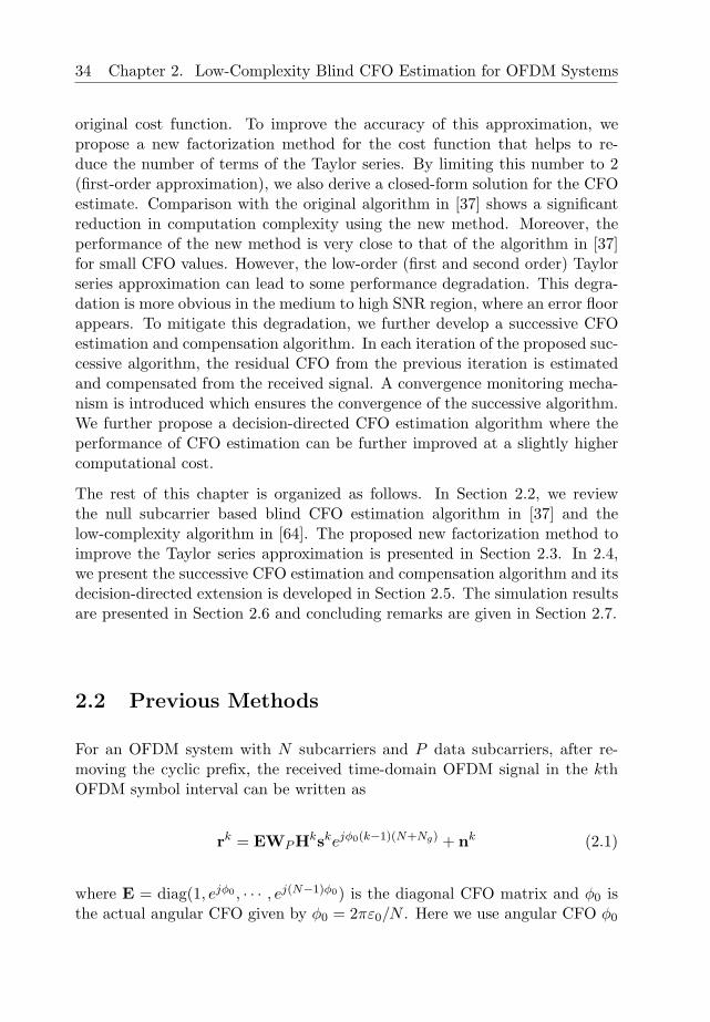
34 Chapter 2. Low-Complexity Blind CFO Estimation for OFDM Systems
original cost function. To improve the accuracy of this approximation, wepropose a new factorization method for the cost function that helps to re-duce the number of terms of the Taylor series. By limiting this number to 2(first-order approximation), we also derive a closed-form solution for the CFOestimate. Comparison with the original algorithm in [37] shows a significantreduction in computation complexity using the new method. Moreover, theperformance of the new method is very close to that of the algorithm in [37]for small CFO values. However, the low-order (first and second order) Taylorseries approximation can lead to some performance degradation. This degra-dation is more obvious in the medium to high SNR region, where an error floorappears. To mitigate this degradation, we further develop a successive CFOestimation and compensation algorithm. In each iteration of the proposed suc-cessive algorithm, the residual CFO from the previous iteration is estimatedand compensated from the received signal. A convergence monitoring mecha-nism is introduced which ensures the convergence of the successive algorithm.We further propose a decision-directed CFO estimation algorithm where theperformance of CFO estimation can be further improved at a slightly highercomputational cost.
The rest of this chapter is organized as follows. In Section 2.2, we reviewthe null subcarrier based blind CFO estimation algorithm in [37] and thelow-complexity algorithm in [64]. The proposed new factorization method toimprove the Taylor series approximation is presented in Section 2.3. In 2.4,we present the successive CFO estimation and compensation algorithm and itsdecision-directed extension is developed in Section 2.5. The simulation resultsare presented in Section 2.6 and concluding remarks are given in Section 2.7.
2.2 Previous Methods
For an OFDM system with N subcarriers and P data subcarriers, after re-moving the cyclic prefix, the received time-domain OFDM signal in the kthOFDM symbol interval can be written as
rk = EWPHkskejφ0(k−1)(N+Ng) + nk (2.1)
where E = diag(1, ejφ0 , · · · , ej(N−1)φ0) is the diagonal CFO matrix and φ0 isthe actual angular CFO given by φ0 = 2πε0/N . Here we use angular CFO φ0
2.2 Previous Methods 35
to simplify notification so that in later derivations, we need not deal with theconstant factor 2π/N to the original CFO ε. The difference between (2.1) and(1.10) is that s is a P × 1 vector containing the transmitted signal on the Pdata subcarriers. Correspondingly, H is a P × P diagonal matrix containingthe channel responses on the P data subcarriers and WP is a N×P submatrixthat is obtained from the N×N IDFT matrix W by extracting the P columnsthat correspond to the data subcarriers. Let us define l = [l1, l2, · · · ld] as thenull subcarrier indices and d = N − P as the number of null subcarriers.
In [37], Liu and Tureli showed that a CFO estimate can be obtained from theminimization of a cost function J (z) given by
J (z) =K∑
k=1
d∑
i=1
∥∥∥wHliZ−1rk
∥∥∥2, (2.2)
where K is the total number of OFDM symbols used for CFO estimation, wHli
is the lith row of the DFT matrix and Z = diag(1, z, z2, · · · , z(N−1)
)with
z = ejφ. Here φ is the trial value for the actual CFO φ0. Using (2.2), it canbe shown that z = ejφ0 is a zero of J (z) in the absence of noise.
This algorithm is shown to have a good performance as compared to Cramer-Rao bound (CRB) [37] and its acquisition range for CFO is much larger thanthat of the blind CFO estimation algorithm using the cyclic prefix [47]. It isshown in [37] that the CFO estimate that minimizes the cost function in (2.2)can be attained by using either a MUSIC-like search algorithm or a rootingmethod. The practical aspects of this blind CFO estimation algorithm and itsexperimental implementations are further studied in [65]. The identifiability ofCFO using this algorithm is studied in [48] and [66]. A major disadvantage ofthis algorithm is its high computational complexity. The cost function J (z)represents a polynomial of order 2(N − 1) in the complex variable z. Fora typical application, like wireless LAN (IEEE 802.11a standard), N = 64.Hence, the order of J (z) becomes 126, and the computational complexityrequired to find its roots is very high. To reduce this complexity, an ESPRIT-like method is proposed in [67]. However, the computational complexity isstill very high as a subspace computation is required.
In [64], a method is proposed to reduce the computational complexity of themethod in [37]. This algorithm exploits the fact that the inverse diagonal
36 Chapter 2. Low-Complexity Blind CFO Estimation for OFDM Systems
matrix Z−1 in (2.2) can be re-written as follows
Z−1 = diag(1, e−jφ, e−j2φ, · · · , e−j(N−1)φ
)
= e−jφ(N−1)/2diag(ejφ
(N−1)2 , ejφ
(N−3)2 , · · · , ejφ
(1−N)2
).
(2.3)
Taking into account the fact that the residual CFO after analog coarse fre-quency synchronization tends to be very small in practice, using Taylor seriesexpansion of an exponential function, we have
Z−1 ≈ e−jφ(N−1)/2 ×Q∑
n=0
(jφ)n
2nn!Dn (2.4)
where D = diag((N − 1), (N − 3), · · · , (1 − N)) and Q is a suitable integer(Q ¿ N) such that the error due to the series truncation in (2.4) is negligible[64]. The assumption of small residual CFO in the digital domain is justified,on the one hand, by the use of a coarse synchronization at the analog partof the receiver [36] [68] and, on the other hand, by the precision of currentlyavailable crystal oscillators [69]. In IEEE 802.11a WLAN standard [17], theprecision of the carrier frequency at both the transmitter and the receiver is±20 ppm maximum. This leads to a worst case CFO value of ±0.64 subcarrierspacing or φ0 = 0.063 at a carrier frequency of fc = 5 GHz. Furthermore,the accuracy of the LO’s has been further improved in recent years. In thecomparison criterion document of the IEEE 802.11n high-throughput wirelessLAN working group [70], the CFO value between the transmitter and receiverLO’s has been strengthened to 13.675 ppm which corresponds to normalizedCFO value of φ0 = 0.023 at fc = 5 GHz. All these facts show that theassumption of |φ| ¿ 1 is valid in practice. Now using (2.4) in (2.2) and lettingai,n(k) = wH
liDnrk, we get the approximated cost function given by
J2Q(φ) =2Q∑
l=0
clφl (2.5)
where the polynomial coefficients cl are given by
2.3 Proposed New Factorization Method 37
cl =(
j
2
)l l∑
m=0
(−1)m
(l −m)!m!
d∑
i=1
K∑
k=1
ai,l−m(k)a∗i,m(k) (2.6)
with ai,l(k) = 0 for l > Q. The new cost function (2.5) is a polynomial ofthe real variable φ of degree 2Q. In addition, it has been proven in [64] thatall the polynomial coefficients are real-valued. The minimization of (2.5) canbe carried out by setting the derivative to 0 and using some standard rootingmethods to search for the CFO estimate. Since Q ¿ N , the computationalcomplexity required to find the root of (2.5) is significantly lower than thatfor the original problem. Moreover, as both φ and the polynomial coefficientsare real, the rooting methods require only real arithmetic operations. This onits own provides large computational savings.
2.3 Proposed New Factorization Method
The factorization in (2.3) is aimed at increasing the denominators of the Taylorseries terms in (2.4) by a factor of 2n so that a good approximation to Z−1 canbe achieved with a limited number of terms. Next, we will propose anotherfactorization method which allows us to increase this number to (2n)2 = 4n
and more if needed. Based on (2.3), we can write
Z−1 = e−jφ(N−1)/2(E1 + E2), (2.7)
where
E1 = diag(ejφ
(N−1)2 , ejφ
(N−3)2 , · · · , ejφ 1
2 , 0, · · · , 0)
= ejφ(N−1)/4diag(ejφ
(N−1)4 , · · · , ejφ
(3−N)4 , 0, · · · , 0
),
E2 = diag(0, · · · , 0, e−jφ 1
2 · · · , ejφ(1−N)
2
)
= ejφ(1−N)/4diag(0, · · · , 0, ejφ
(N−3)4 , · · · , ejφ
(1−N)4
). (2.8)
38 Chapter 2. Low-Complexity Blind CFO Estimation for OFDM Systems
Now, using Taylor series expansion in (2.8), we obtain
E1 =+∞∑
m=0
(jφ)m
4mm!(N − 1)m
+∞∑
n=0
(jφ)n
4nn!Dn
1
=+∞∑
m=0
+∞∑
n=0
(jφ)n+m
4n+mn!m!(N − 1)mDn
1 ,
(2.9)
where
Dn1 = diag((N − 1)n, (N − 5)n, · · · (3−N)n, 0, · · · , 0). (2.10)
Similarly, we can show that
E2 =+∞∑
m=0
+∞∑
n=0
(−1)m (jφ)n+m
4n+mn!m!(N − 1)mDn
2 , (2.11)
where
Dn2 = diag(0, · · · , 0, (N − 3)n, (N − 7)n, · · · (1−N)n). (2.12)
Substituting (2.9) and (2.11) into (2.7) leads to
Z−1 = ejφ(N−1)/2+∞∑
m=0
+∞∑
n=0
(jφ)n+m
4n+mn!m!(N − 1)m [Dn
1 + (−1)mDn2 ] . (2.13)
If the Taylor series of each exponential is truncated to a suitable number ofQ terms, then equation (2.13) can be approximated by the following matrixpolynomial
Z−1 ≈ ejφ(N−1)/22Q∑
q=0
Cqφq, (2.14)
2.3 Proposed New Factorization Method 39
where
Cq =(
j
4
)q q∑
m=0
(N − 1)m
m!(q −m)!
[D(q−m)
1 + (−1)mD(q−m)2
]. (2.15)
Note that Cq is a non-zero matrix for q = 0, 1, · · · 2Q and it is equal to thezero-matrix for q > 2Q. To simplify the calculations, let us define the scalarbi,q(k) as follows
bi,q(k) = wHliCqrk. (2.16)
Now, let us substitute (2.14) into the cost function (2.2). This leads to thenew approximate cost function
J (z = ejφ) ≈ J4Q(φ) =2Q∑
r=0
2Q∑
l=0
φl+rd∑
i=1
K∑
k=1
bi,l(k)b∗i,r(k)
=4Q∑
q=0
dqφq,
(2.17)
where the polynomial coefficients are given by
dq =q∑
s=0
d∑
i=1
K∑
k=1
bi,q−s(k)b∗i,s(k). (2.18)
We can notice that bi,l(k) = 0 for l > 2Q as Cl is a zero matrix for l > 2Q.Moreover, it is straightforward to show that dq = d∗q . Hence, all the coefficientsof the polynomial are real-valued.
In practice, the residual CFO can be so small that only a very limited numberof terms is needed for the Taylor series approximation. In this case, we cancompute directly the CFO through a simple formula as follows. For Q = 1,the cost function polynomial is of degree four and its derivative with respect toφ is a cubic polynomial whose zeroes or roots can be computed directly usingCardano’s formula [71]. To this end, we should first rewrite the derivative of
40 Chapter 2. Low-Complexity Blind CFO Estimation for OFDM Systems
the cost function as follows:
14d4
∂J4Q(φ)∂φ
= φ3 + uφ2 + vφ + r = 0, (2.19)
whereu =
3d3
4d4, v =
d2
2d4, r =
d1
4d4. (2.20)
Now, let us compute
a = (3v − u2)/3, b = (2u3 − 9uv + 27r)/27,
S =
(− b
2+
√b2
4+
a3
27
)1/3
, T =
(− b
2−
√b2
4+
a3
27
)1/3
.
(2.21)Finally, the three roots are given by [71]
φ1 = (S + T )− u
3,
φ2 = −12(S + T ) + j
√3
2(S − T )− u
3,
φ3 = −12(S + T )− j
√3
2(S − T )− u
3.
(2.22)
Once the three roots are determined, we substitute them in (2.17) and choosethe one that leads to the minimum of J4(φ) as the CFO estimate. As we arelooking for a real solution, we should test only the real roots for the minimum.The complex-valued roots need not be tested. It is worthwhile to mentionthat for a cubic polynomial with real coefficients as in our case, at least oneof the roots will always be real [72]. The summary of this algorithm is givenin Table 2.1.
To complete our discussion, we need to examine closely the computationalcomplexity of the proposed algorithm. Since Q = 1, the computational com-plexity due to (2.20), (2.21) and (2.22) is negligible as compared to the com-plexity of computing the 5 polynomial coefficients d0 to d4. Every coefficientdq requires the computation of bi,q(k) in (2.16), where we can easily noticethat Cq is just a diagonal matrix and both wH
liand y(k) are just vectors.
As a result, the computational complexity for obtaining the polynomial coef-
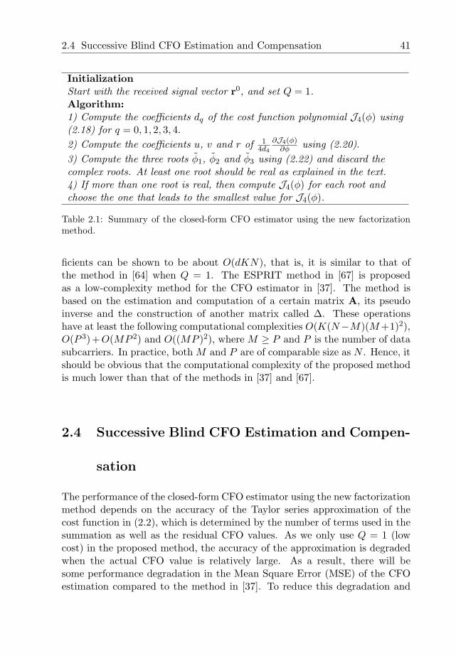
2.4 Successive Blind CFO Estimation and Compensation 41
InitializationStart with the received signal vector r0, and set Q = 1.Algorithm:1) Compute the coefficients dq of the cost function polynomial J4(φ) using(2.18) for q = 0, 1, 2, 3, 4.2) Compute the coefficients u, v and r of 1
4d4
∂J4(φ)∂φ using (2.20).
3) Compute the three roots φ1, φ2 and φ3 using (2.22) and discard thecomplex roots. At least one root should be real as explained in the text.4) If more than one root is real, then compute J4(φ) for each root andchoose the one that leads to the smallest value for J4(φ).
Table 2.1: Summary of the closed-form CFO estimator using the new factorizationmethod.
ficients can be shown to be about O(dKN), that is, it is similar to that ofthe method in [64] when Q = 1. The ESPRIT method in [67] is proposedas a low-complexity method for the CFO estimator in [37]. The method isbased on the estimation and computation of a certain matrix A, its pseudoinverse and the construction of another matrix called ∆. These operationshave at least the following computational complexities O(K(N−M)(M +1)2),O(P 3)+O(MP 2) and O((MP )2), where M ≥ P and P is the number of datasubcarriers. In practice, both M and P are of comparable size as N . Hence, itshould be obvious that the computational complexity of the proposed methodis much lower than that of the methods in [37] and [67].
2.4 Successive Blind CFO Estimation and Compen-
sation
The performance of the closed-form CFO estimator using the new factorizationmethod depends on the accuracy of the Taylor series approximation of thecost function in (2.2), which is determined by the number of terms used in thesummation as well as the residual CFO values. As we only use Q = 1 (lowcost) in the proposed method, the accuracy of the approximation is degradedwhen the actual CFO value is relatively large. As a result, there will besome performance degradation in the Mean Square Error (MSE) of the CFOestimation compared to the method in [37]. To reduce this degradation and
42 Chapter 2. Low-Complexity Blind CFO Estimation for OFDM Systems
further improve the performance of the proposed method, we present, in thissection, an effective successive CFO estimation and compensation algorithm.
In the first iteration of the algorithm, we use the proposed method to findan initial estimate of the CFO, say φ0. Then, the CFO compensation can beperformed on the received signal rk. To this end, let us define the CFO com-pensation matrix in the first iteration as T1 = diag(1, e−jφ0 , · · · , e−j(N−1)φ0).The time-domain received signal after the CFO compensation can thus bewritten as
rk = T1e−jφ0(k−1)(N+Ng)rk
= E1WPHskejφ1(k−1)(N+Ng) +(nk
)′, (2.23)
where E1 = diag(1, ejφ1 , ej2φ1 , · · · , ej(N−1)φ1) denotes the residual CFO matrixwith φ1 = φ0− φ0 representing the residual CFO after the first iteration. Thenoise vector
(nk
)′ = T1e−jφ0(k−1)(N+Ng)nk.
Let us consider the residual CFO after the first iteration E1ejφ1(k−1)(N+Ng) in
(2.23). It is obvious that when the CFO estimation is perfect, we should haveφ0 = φ0 and φ1 = 0. In this case, we have E1e
jφ1(k−1)(N+Ng) = I. Next, weconsider the case where the CFO is not perfectly estimated (φ0 6= φ0) but itis close enough to φ0 for the following condition to hold
|φ1| =∣∣∣φ0 − φ0
∣∣∣ < |φ0| . (2.24)
Note that the mean of the noise term n′(k) after CFO compensation is E(n′(k)) =0 = E(n(k)), and its covariance matrix can be calculated as
R = E(T1e
−jφ0(k−1)(N+Ng)nk(nk
)Hejφ0(k−1)(N+Ng)TH
1
)
= T1e−jφ0(k−1)(N+Ng)E
(nk
(nk
)H)
ejφ0(k−1)(N+Ng)T1H
= σ2nT1e
−jφ0(k−1)(N+Ng)Iejφ0(k−1)(N+Ng)TH1
= σ2nI, (2.25)
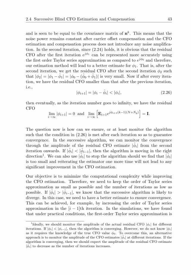
2.4 Successive Blind CFO Estimation and Compensation 43
and is seen to be equal to the covariance matrix of nk. This means that thenoise power remains constant after carrier offset compensation and the CFOestimation and compensation process does not introduce any noise amplifica-tion. In the second iteration, since (2.24) holds, it is obvious that the residualCFO after the first iteration ejφ1 can be represented more accurately usingthe first order Taylor series approximation as compared to ejφ0 and therefore,our estimation method will lead to a better estimate for φ1. That is, after thesecond iteration, we get the residual CFO after the second iteration φ2 suchthat |φ2| = |φ1− φ1| = |φ0− (φ0 + φ1)| is very small. Now if after every itera-tion, we have the residual CFO smaller than that after the previous iteration,i.e.,
|φi+1| = |φi − φi| < |φi|, (2.26)
then eventually, as the iteration number goes to infinity, we have the residualCFO
limi→∞
|φi+1| = 0 and limi→∞
[Ei+1e
jφi+1(k−1)(N+Ng)]
= I.
The question now is how can we ensure, or at least monitor the algorithmsuch that the condition in (2.26) is met after each iteration so as to guaranteeconvergence. In the successive algorithm, we can monitor the convergencethrough the amplitude of the residual CFO estimate |φi| from the seconditeration onwards. If |φi| < |φi−1|, then the algorithm is moving in the rightdirection1. We can also use |φi| to stop the algorithm should we find that |φi|is too small and reiterating the estimator one more time will not lead to anysignificant improvement in the CFO estimation.
Our objective is to minimize the computational complexity while improvingthe CFO estimation. Therefore, we need to keep the order of Taylor seriesapproximation as small as possible and the number of iterations as low aspossible. If |φi| > |φi−1|, we know that the successive algorithm is likely todiverge. In this case, we need to have a better estimate to ensure convergence.This can be achieved, for example, by increasing the order of Taylor seriesapproximation in the [i − 1]th iteration. In the simulations, we have foundthat under practical conditions, the first-order Taylor series approximation is
1Ideally, we should monitor the amplitude of the actual residual CFO |φi| for differentiterations. If |φi| < |φi−1|, then the algorithm is converging. However, we do not know |φi|as it requires the knowledge of the true CFO value φ0. To overcome this, an alternativeapproach is to monitor the amplitude of the CFO estimates |φi| at different iterations. If thealgorithm is converging, then we should expect the amplitude of the residual CFO estimate|φi| to decrease as the number of iterations increases.
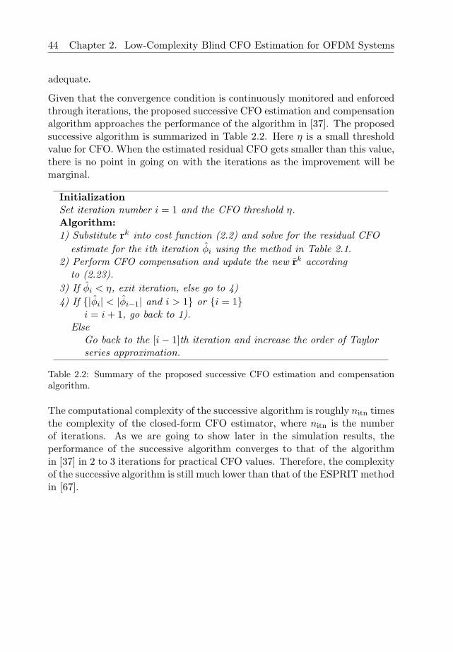
44 Chapter 2. Low-Complexity Blind CFO Estimation for OFDM Systems
adequate.
Given that the convergence condition is continuously monitored and enforcedthrough iterations, the proposed successive CFO estimation and compensationalgorithm approaches the performance of the algorithm in [37]. The proposedsuccessive algorithm is summarized in Table 2.2. Here η is a small thresholdvalue for CFO. When the estimated residual CFO gets smaller than this value,there is no point in going on with the iterations as the improvement will bemarginal.
InitializationSet iteration number i = 1 and the CFO threshold η.Algorithm:1) Substitute rk into cost function (2.2) and solve for the residual CFO
estimate for the ith iteration φi using the method in Table 2.1.2) Perform CFO compensation and update the new rk according
to (2.23).3) If φi < η, exit iteration, else go to 4)4) If |φi| < |φi−1| and i > 1 or i = 1
i = i + 1, go back to 1).Else
Go back to the [i− 1]th iteration and increase the order of Taylorseries approximation.
Table 2.2: Summary of the proposed successive CFO estimation and compensationalgorithm.
The computational complexity of the successive algorithm is roughly nitn timesthe complexity of the closed-form CFO estimator, where nitn is the numberof iterations. As we are going to show later in the simulation results, theperformance of the successive algorithm converges to that of the algorithmin [37] in 2 to 3 iterations for practical CFO values. Therefore, the complexityof the successive algorithm is still much lower than that of the ESPRIT methodin [67].
2.5 Decision-directed Successive Algorithm 45
2.5 Decision-directed Successive Algorithm
Due to averaging, the MSE of the CFO estimation gets smaller as the numberof null subcarriers, i.e., d used in cost function (2.2), gets larger. In practice,we cannot afford to have many null subcarriers in one OFDM symbol as thisreduces the bandwidth efficiency. However, if the CFO estimation is accuratein the initial iteration, by performing CFO compensation and OFDM detectionon a set of high SNR data subcarriers, we are able to obtain relatively accurateestimates sk of the transmitted signals sk on these high-SNR subcarriers. Here,in order to keep the computational complexity low, we limit ourselves to thecase where only 1 OFDM symbol is used for CFO estimation, i.e. K = 1 as in(2.2)and later in the simulation results section, we will show that K = 1 givesus good performance for all the proposed algorithms. In this case, we can dropthe OFDM symbol index k in all the following formulations. Let us denotethe selected high-SNR data subcarriers as d and the set of null subcarriersas l. We can thus use a decision-directed method and re-formulate the costfunction as
J (z) =∑
i∈d
∥∥wHi Z−1r− hisi
∥∥2+
∑
i∈l
∥∥wHi Z−1r
∥∥2, (2.27)
where hi, si are the channel response and detected signal on subcarrier i.The two terms in the summation in (2.27) correspond to the cost functionon the selected data subcarriers and the null subcarriers. Using Taylor seriesexpansion as before, the decision-directed cost function is given by
J (φ) =∑
i∈d
∥∥∥∥∥wHi
+∞∑
n=0
(jφ)n
n!Dn
dr− hisi
∥∥∥∥∥
2
+ J4Q(φ), (2.28)
where Dd = diag(0,−1,−2, · · · , 1−N) and here we use subscript d to denotedecision-directed. The function J4Q(φ) is the same cost function on the nullsubcarriers given in (2.17). Comparing (2.28) to (2.3), we can see that forthe data subcarriers, we can no longer bring e−jφ
(N−1)2 out of the modulus
operation. Therefore, in the Taylor series summation, we do not have the 2n
term in the denominator. As a result, the amplitudes of higher-order terms donot decay as fast as for (2.2) and we need to include more terms in the Taylorseries summation in order to get a good approximation of Z−1.
46 Chapter 2. Low-Complexity Blind CFO Estimation for OFDM Systems
Suppose we use M terms in the Taylors series approximation and set ai,n =wH
i Dndr, then the cost function in (2.28) can be expanded as
J (φ) =∑
i∈d
[M∑
n=0
M∑
m=0
(jφ)n
n!((jφ)m)∗
m!ai,na∗i,m
−2Re
(M∑
n=1
(jφ)n
n!ai,n (h(i)s(i))∗
)+ |hisi|2
]+ J4Q(φ),
(2.29)
where Re(•) denotes the real part of a complex number. Here, we assumethe channel to be known at the receiver 2. In practice, the decision-directedmethod is only invoked starting from the second iteration onwards as thedetected symbol is only available after the first iteration. That means thatan initial CFO estimate is already obtained in the first iteration. Therefore,what the decision-directed method needs to estimate is only the residual CFO,which is much smaller than φ0. Note that the cost function of data subcarriersis a function of φ with order 2M . In practice, we can set M = 2 such that thecost functions of the data subcarriers and the null subcarriers are both of order4. The overall cost function in (2.29) is therefore also order 4 and we can usethe proposed closed-form solution to find the φ that minimizes the total cost.However, the coefficients of the polynomial need to be re-calculated accordingto (2.29). Note that to ensure convergence of the algorithm, we again need tomonitor the amplitude of the CFO estimate |φi| after different iterations.
The complexity of the decision-directed blind CFO estimation technique ishigher because more subcarriers are used in the cost function calculation. Inpractice, the size of d should be chosen such that a good trade-off betweencomplexity and performance is achieved. The decision-directed CFO estima-tion algorithm can be summarized as shown in Table 2.3.
2The channel can also be estimated blindly using blind channel estimation methods suchas [73].
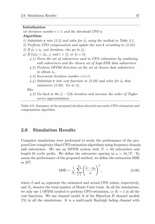
2.6 Simulation Results 47
Initializationset iteration number i = 1 and the threshold CFO ηAlgorithm:1) Substitute r into (2.2) and solve for φi using the method in Table 2.1.2) Perform CFO compensation and update the new r according to (2.23).3) If φi < η, exit iteration, else go to 4).4) If |φi| < |φi−1| and i > 1 or i = 1
4.1) Form the set of subcarriers used in CFO estimation by combiningnull subcarriers and the chosen set of high-SNR data subcarriers.
4.2) Perform OFDM detection on the set of chosen data subcarriersto obtain si.
4.3) Increment iteration number i=i+1.4.4) Substitute r into cost function in (2.29) and solve for φi that
minimizes (2.29). Go to 2).Else
4.5) Go back to the [i− 1]th iteration and increase the order of Taylorseries approximation.
Table 2.3: Summary of the proposed decision-directed successive CFO estimation andcompensation algorithm.
2.6 Simulation Results
Computer simulations were performed to study the performance of the pro-posed low-complexity blind CFO estimation algorithms using frequency-domainnull subcarriers. We use an OFDM system with N = 64 subcarriers andlength-16 cyclic prefix. We define the subcarrier spacing as ω = 2π/N . Toassess the performance of the proposed method, we define the estimation MSEas [67]
MSE =1
Ns
Ns∑
i=1
(φ− φ0
ω
)2
, (2.30)
where φ and φ0 represent the estimated and actual CFO values, respectively,and Ns denotes the total number of Monte Carlo trials. In all the simulations,we only use 1 OFDM symbol to perform CFO estimation, i.e K = 1 in all thecost functions. We use channel model A of the HiperLan II channel models[74] in all the simulations. It is a multi-path Rayleigh fading channel with
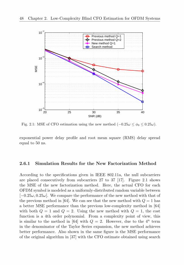
48 Chapter 2. Low-Complexity Blind CFO Estimation for OFDM Systems
20 25 30 35 4010
−5
10−4
10−3
10−2
SNR (dB)
MS
E
Previous method Q=1Previous method Q=2New method Q=1Search method
Fig. 2.1: MSE of CFO estimation using the new method (−0.25ω ≤ φ0 ≤ 0.25ω).
exponential power delay profile and root mean square (RMS) delay spreadequal to 50 ns.
2.6.1 Simulation Results for the New Factorization Method
According to the specifications given in IEEE 802.11a, the null subcarriersare placed consecutively from subcarriers 27 to 37 [17]. Figure 2.1 showsthe MSE of the new factorization method. Here, the actual CFO for eachOFDM symbol is modeled as a uniformly-distributed random variable between[−0.25ω, 0.25ω]. We compare the performance of the new method with that ofthe previous method in [64]. We can see that the new method with Q = 1 hasa better MSE performance than the previous low-complexity method in [64]with both Q = 1 and Q = 2. Using the new method with Q = 1, the costfunction is a 4th order polynomial. From a complexity point of view, thisis similar to the method in [64] with Q = 2. However, due to the 4n termin the denominator of the Taylor Series expansion, the new method achievesbetter performance. Also shown in the same figure is the MSE performanceof the original algorithm in [37] with the CFO estimate obtained using search
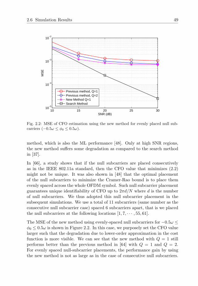
2.6 Simulation Results 49
10 15 20 25 3010
−5
10−4
10−3
10−2
SNR (dB)
MS
E
Previous method, Q=1Previous method, Q=2New Method Q=1Search Method
Fig. 2.2: MSE of CFO estimation using the new method for evenly placed null sub-carriers (−0.5ω ≤ φ0 ≤ 0.5ω).
method, which is also the ML performance [48]. Only at high SNR regions,the new method suffers some degradation as compared to the search methodin [37].
In [66], a study shows that if the null subcarriers are placed consecutivelyas in the IEEE 802.11a standard, then the CFO value that minimizes (2.2)might not be unique. It was also shown in [48] that the optimal placementof the null subcarriers to minimize the Cramer-Rao bound is to place themevenly spaced across the whole OFDM symbol. Such null subcarrier placementguarantees unique identifiability of CFO up to 2πd/N where d is the numberof null subcarriers. We thus adopted this null subcarrier placement in thesubsequent simulations. We use a total of 11 subcarriers (same number as theconsecutive null subcarrier case) spaced 6 subcarriers apart, that is we placedthe null subcarriers at the following locations [1, 7, · · · , 55, 61].
The MSE of the new method using evenly-spaced null subcarriers for −0.5ω ≤φ0 ≤ 0.5ω is shown in Figure 2.2. In this case, we purposely set the CFO valuelarger such that the degradation due to lower-order approximation in the costfunction is more visible. We can see that the new method with Q = 1 stillperforms better than the previous method in [64] with Q = 1 and Q = 2.For evenly spaced null-subcarrier placements, the performance gain by usingthe new method is not as large as in the case of consecutive null subcarriers.
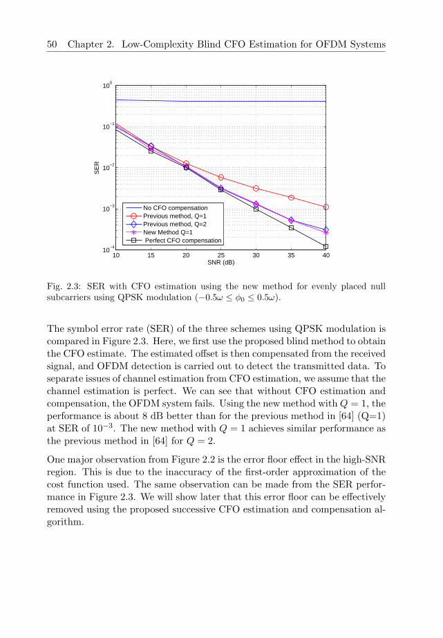
50 Chapter 2. Low-Complexity Blind CFO Estimation for OFDM Systems
10 15 20 25 30 35 4010
−4
10−3
10−2
10−1
100
SNR (dB)
SE
R
No CFO compensationPrevious method, Q=1Previous method, Q=2New Method Q=1 Perfect CFO compensation
Fig. 2.3: SER with CFO estimation using the new method for evenly placed nullsubcarriers using QPSK modulation (−0.5ω ≤ φ0 ≤ 0.5ω).
The symbol error rate (SER) of the three schemes using QPSK modulation iscompared in Figure 2.3. Here, we first use the proposed blind method to obtainthe CFO estimate. The estimated offset is then compensated from the receivedsignal, and OFDM detection is carried out to detect the transmitted data. Toseparate issues of channel estimation from CFO estimation, we assume that thechannel estimation is perfect. We can see that without CFO estimation andcompensation, the OFDM system fails. Using the new method with Q = 1, theperformance is about 8 dB better than for the previous method in [64] (Q=1)at SER of 10−3. The new method with Q = 1 achieves similar performance asthe previous method in [64] for Q = 2.
One major observation from Figure 2.2 is the error floor effect in the high-SNRregion. This is due to the inaccuracy of the first-order approximation of thecost function used. The same observation can be made from the SER perfor-mance in Figure 2.3. We will show later that this error floor can be effectivelyremoved using the proposed successive CFO estimation and compensation al-gorithm.
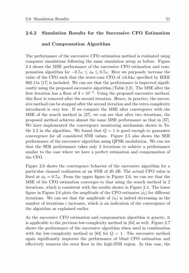
2.6 Simulation Results 51
2.6.2 Simulation Results for the Successive CFO Estimation
and Compensation Algorithm
The performance of the successive CFO estimation method is evaluated usingcomputer simulations following the same simulation setup as before. Figure2.4 shows the MSE performance of the successive CFO estimation and com-pensation algorithm for −0.7ω ≤ φ0 ≤ 0.7ω. Here we purposely increase thevalue of the CFO such that the worst-case CFO of ±0.64ω specified by IEEE802.11a [17] is included. We can see that the performance is improved signifi-cantly using the proposed successive algorithm (Table 2.2). The MSE after thefirst iteration has a floor of 3× 10⁻³. Using the proposed successive method,this floor is removed after the second iteration. Hence, in practice, the succes-sive method can be stopped after the second iteration and the extra complexityintroduced is very low. If we compare the MSE after convergence with theMSE of the search method in [37], we can see that after two iterations, theproposed method achieves almost the same MSE performance as that in [37].We have implemented the convergence monitoring mechanism shown in Ta-ble 2.2 in the algorithm. We found that Q = 1 is good enough to guaranteeconvergence for all considered SNR values. Figure 2.5 also shows the SERperformance of the successive algorithm using QPSK modulation. We can seethat the SER performance takes only 2 iterations to achieve a performancesimilar to the case where we have a perfect estimation and compensation ofthe CFO.
Figure 2.6 shows the convergence behavior of the successive algorithm for aparticular channel realization at an SNR of 20 dB. The actual CFO value isfixed at φ0 = 0.7ω. From the upper figure in Figure 2.6, we can see that theMSE of the CFO estimation converges to that using the search method in 2iterations, which is consistent with the results shown in Figure 2.4. The lowerfigure in Figure 2.6 plots the amplitude of the CFO estimates |φi| for differentiterations. We can see that the amplitude of |φi| is indeed decreasing as thenumber of iterations i increases, which is an indication of the convergence ofthe algorithm as explained earlier.
As the successive CFO estimation and compensation algorithm is generic, itis applicable to the previous low-complexity method in [64] as well. Figure 2.7shows the performance of the successive algorithm when used in combinationwith the low-complexity method in [64] for Q = 1. The successive methodagain significantly improves the performance of blind CFO estimation andeffectively removes the error floor in the high-SNR region. In this case, the
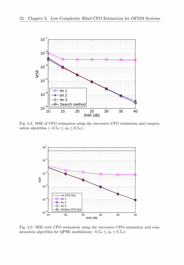
52 Chapter 2. Low-Complexity Blind CFO Estimation for OFDM Systems
10 15 20 25 30 35 4010
−6
10−5
10−4
10−3
10−2
10−1
SNR (dB)
MS
E
itn 1itn 2itn 3Search method
Fig. 2.4: MSE of CFO estimation using the successive CFO estimation and compen-sation algorithm (−0.7ω ≤ φ0 ≤ 0.7ω).
15 20 25 30 35 4010
−5
10−4
10−3
10−2
10−1
100
SNR (dB)
SE
R
no CFO Estitn 1itn 2itn 3Perfect CFO Est
Fig. 2.5: SER with CFO estimation using the successive CFO estimation and com-pensation algorithm for QPSK modulation(−0.7ω ≤ φ0 ≤ 0.7ω).
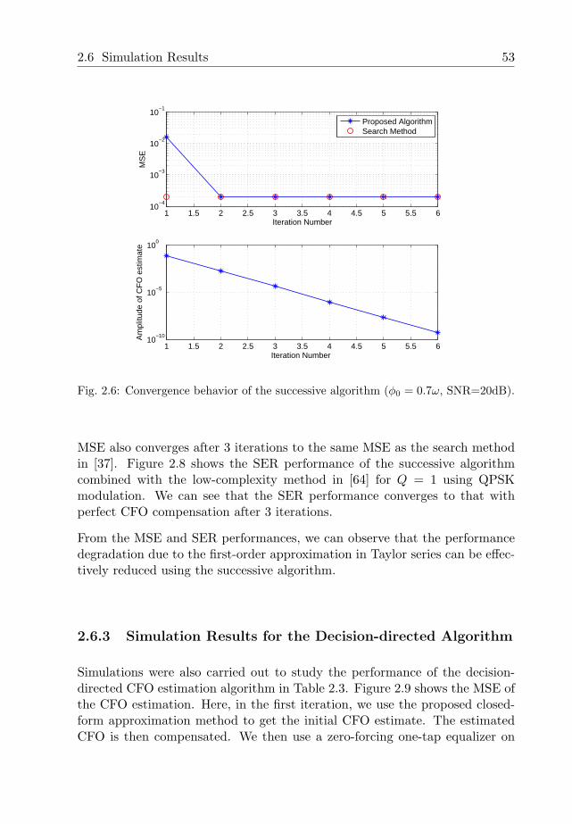
2.6 Simulation Results 53
1 1.5 2 2.5 3 3.5 4 4.5 5 5.5 610
−4
10−3
10−2
10−1
Iteration Number
MS
E
Proposed AlgorithmSearch Method
1 1.5 2 2.5 3 3.5 4 4.5 5 5.5 610
−10
10−5
100
Iteration Number
Am
plitu
de o
f CF
O e
stim
ate
Fig. 2.6: Convergence behavior of the successive algorithm (φ0 = 0.7ω, SNR=20dB).
MSE also converges after 3 iterations to the same MSE as the search methodin [37]. Figure 2.8 shows the SER performance of the successive algorithmcombined with the low-complexity method in [64] for Q = 1 using QPSKmodulation. We can see that the SER performance converges to that withperfect CFO compensation after 3 iterations.
From the MSE and SER performances, we can observe that the performancedegradation due to the first-order approximation in Taylor series can be effec-tively reduced using the successive algorithm.
2.6.3 Simulation Results for the Decision-directed Algorithm
Simulations were also carried out to study the performance of the decision-directed CFO estimation algorithm in Table 2.3. Figure 2.9 shows the MSE ofthe CFO estimation. Here, in the first iteration, we use the proposed closed-form approximation method to get the initial CFO estimate. The estimatedCFO is then compensated. We then use a zero-forcing one-tap equalizer on
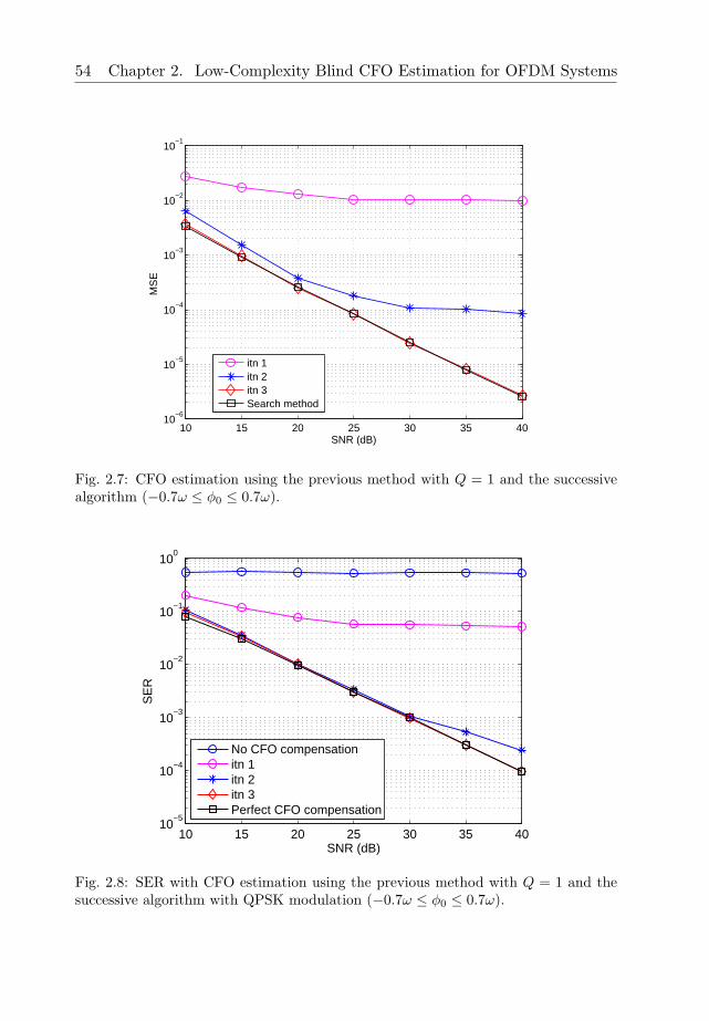
54 Chapter 2. Low-Complexity Blind CFO Estimation for OFDM Systems
10 15 20 25 30 35 4010
−6
10−5
10−4
10−3
10−2
10−1
SNR (dB)
MS
E
itn 1itn 2itn 3Search method
Fig. 2.7: CFO estimation using the previous method with Q = 1 and the successivealgorithm (−0.7ω ≤ φ0 ≤ 0.7ω).
10 15 20 25 30 35 4010
−5
10−4
10−3
10−2
10−1
100
SNR (dB)
SE
R
No CFO compensationitn 1itn 2itn 3Perfect CFO compensation
Fig. 2.8: SER with CFO estimation using the previous method with Q = 1 and thesuccessive algorithm with QPSK modulation (−0.7ω ≤ φ0 ≤ 0.7ω).
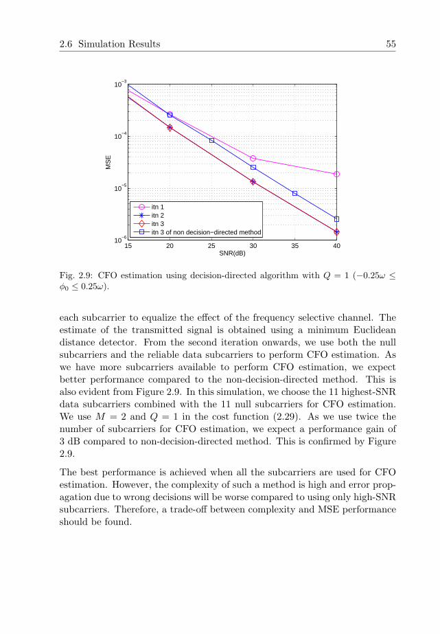
2.6 Simulation Results 55
15 20 25 30 35 4010
−6
10−5
10−4
10−3
SNR(dB)
MS
E
itn 1itn 2itn 3itn 3 of non decision−directed method
Fig. 2.9: CFO estimation using decision-directed algorithm with Q = 1 (−0.25ω ≤φ0 ≤ 0.25ω).
each subcarrier to equalize the effect of the frequency selective channel. Theestimate of the transmitted signal is obtained using a minimum Euclideandistance detector. From the second iteration onwards, we use both the nullsubcarriers and the reliable data subcarriers to perform CFO estimation. Aswe have more subcarriers available to perform CFO estimation, we expectbetter performance compared to the non-decision-directed method. This isalso evident from Figure 2.9. In this simulation, we choose the 11 highest-SNRdata subcarriers combined with the 11 null subcarriers for CFO estimation.We use M = 2 and Q = 1 in the cost function (2.29). As we use twice thenumber of subcarriers for CFO estimation, we expect a performance gain of3 dB compared to non-decision-directed method. This is confirmed by Figure2.9.
The best performance is achieved when all the subcarriers are used for CFOestimation. However, the complexity of such a method is high and error prop-agation due to wrong decisions will be worse compared to using only high-SNRsubcarriers. Therefore, a trade-off between complexity and MSE performanceshould be found.
56 Chapter 2. Low-Complexity Blind CFO Estimation for OFDM Systems
2.7 Conclusions
In this chapter, we developed a new factorization method to approximate thecost function for blind CFO estimation in OFDM systems using null subcar-riers. Using this new method, we further derived closed-form solutions for theCFO estimate using a first-order Taylor series approximation. This new CFOestimator reduces the computational complexity of the CFO estimation sig-nificantly. We also proposed a successive CFO estimation and compensationalgorithm which further improves the performance of the new CFO estima-tor. Indeed, using the proposed successive algorithm, we were able to achievesimilar performance as the method in [37] yet at a much lower computationalcomplexity. A decision-directed extension of the successive algorithm was alsogiven, which achieves even better performance at the cost of slightly highercomputational complexity.
Chapter 3Optimal Null Subcarrier Placement
for Blind CFO Estimation
3.1 Introduction
In Chapter 2, we studied the blind CFO estimation algorithm using null sub-carriers by Liu and Tureli [37] and proposed new algorithms to reduce thecomputational complexity when the CFO is small. In this chapter, we presenta mathematical analysis on the relationship between the placement of null sub-carriers and the performance of the CFO estimation. A previous work in [66]showed that consecutively placed null subcarriers at both ends of the spectrumdoes not guarantee unique solution for the CFO estimates. The identifiabilityof the CFO estimator in [37] with different null subcarrier placement is furtherstudied in [48]. Moreover, it was also shown that equally spaced null subcarrierplacement minimizes the Cramer Rao bound (CRB) of the CFO estimation.As the CRB is not always achievable for practical CFO estimation schemes, inthis chapter, we study the relationship between the null subcarrier placementand the following two more practical performance-related parameters
58Chapter 3. Optimal Null Subcarrier Placement for Blind CFO Estimation
• SNR of the CFO estimation;• Theoretical MSE of the CFO estimation, which is a linear approximation
of the actual MSE of CFO estimation in the high SNR region.
Based on the obtained relationship, we find the null subcarrier placement thatmaximizes the SNR and minimizes the theoretical MSE, respectively. We showthat the two optimization problems are equivalent and a single optimal nullsubcarrier placement exists. For the case when the number of subcarriers isdivisible by the number of null subcarriers, the exact optimal placement can befound. Interestingly, this is also the null subcarrier placement that minimizesthe CRB as given in [48]. When the number of subcarriers is not divisibleby the number of null subcarriers, it is difficult to prove the optimality of thenull subcarrier placement due to the integer constraints on the null subcarrierpositions. However, we will develop a heuristic procedure on how to place thenull subcarriers where good performance can still be achieved. We verify thatthe null subcarrier placement obtained using the proposed heuristic procedureis indeed optimal using exhaustive computer search when the number of nullsubcarriers is small. We also extend the optimization problem to a practicalOFDM system where guard bands are required at both ends of the spectrum.In this case, if given a few more null subcarriers that can be inserted freelyin the OFDM symbol, we show how to place them to guarantee the SNRoptimality in the CFO estimation. We show from computer simulations thatwith the proposed null subcarrier placement, the performance of the CFOestimation can be significantly improved. We further show that for practicalOFDM systems with guard bands, introduction of a few extra null subcarriersleads to much better performance of the blind CFO estimation.
The rest of this chapter is organized as follows. In Section 3.2, we study therelationship between the null subcarrier placement and the SNR of the CFOestimation. We find the null subcarrier placement that maximizes this SNR,which we call SNRCFO to distinguish it from the SNR of the received signal. InSection 3.3, we derive the theoretical MSE of the CFO estimation and obtainits relationship with the null subcarrier placement. We then show that thenull subcarrier placement that minimizes the theoretical MSE also maximizesthe SNRCFO. Optimal null subcarrier placement for practical OFDM systemswith guard bands is studied in Section 3.4. In Section 3.5, we present computersimulation results and conclusions are drawn in Section 3.6.
3.2 Placement of Null Subcarriers Based on SNRCFO Maximization 59
3.2 Placement of Null Subcarriers Based on SNRCFO
Maximization
For an OFDM system with a CFO value of ε0, the received frequency domainsignal on a null subcarrier li of OFDM symbol m can be written as
ymli
= wHlirm =
N−1∑
n=0,n6∈lm
hmn sm
n Cmn−li
(ε0) + nmli
= ICImli (ε0) + nmli
, (3.1)
where wHli
is the lith row of the DFT matrix, and rm is the time domainreceived signal for the mth OFDM symbol given in (2.1). We use hm
liand
smli
to denote the channel response and transmitted data on subcarrier li ofOFDM symbol m. Vector lm contains indices of all the null subcarriers inOFDM symbol m. The ICI due to CFO of ε0 on subcarrier li is denoted asICImli (ε0) and nm
liis the AWGN noise. The value of Cm
k (ε0) is given by [75]
Cmk (ε0) =
sin [π(k + ε0)]N sin
[πN (k + ε0)
] exp (jπ(k + ε0)(1− 1/N))
exp (j2πε0(m− 1)(1 + Ng/N)) . (3.2)
Using (3.1), the cost function in (2.2), which is the summation of the receivedsignal power over all the null subcarriers, can be equivalently re-written as
J (ε) =K∑
m=1
d∑
i=1
∣∣∣wHli
diag(1, e−j2πε/N , e−j2π2ε/N , · · · , e−j2π(N−1)ε/N )rm∣∣∣2
=K∑
m=1
d∑
i=1
∣∣ICImli (ε0 − ε) + nmli
∣∣2
=K∑
m=1
d∑
i=1
∣∣∣∣∣∣
N−1∑
n=0,n6∈lm
hmn sm
n Cmn−li
(ε0 − ε) + nmli
∣∣∣∣∣∣
2
.
(3.3)
60Chapter 3. Optimal Null Subcarrier Placement for Blind CFO Estimation
Correspondingly, the estimate of the CFO is given by
ε = arg minεJ (ε). (3.4)
Note that the received signal on a null subcarrier li in (3.1) is the sum of ICImliand nm
li. In these two terms, ICImli is the useful signal term which we can
use to estimate the CFO ε0, and nmli
is the noise term, which is uncorrelatedwith ICImli . Therefore, using (3.1) we can define an objective function, calledSNRCFO as
SNRCFO =E
(∑Km=1
∑di=1
∣∣ICImli (ε0)∣∣2
)
E(∑K
m=1
∑di=1
∣∣∣nmli
∣∣∣2) , (3.5)
where E denotes statistical expectation. Note that the objective function canbe interpreted as the SNR of the CFO estimation. The power of ICI onsubcarrier li in OFDM symbol m can be written as
E∣∣ICImli (ε0)
∣∣2 = E
∣∣∣∣∣∣
N−1∑
n=0,n6∈lm
hmn sm
n Cmn−li
(ε0)
∣∣∣∣∣∣
2
=
N−1∑
n=0,n6∈lm
E|hmn sm
n |2sin2 [π(n− li + ε0)]
N2 sin2[
πN (n− li + ε0)
] . (3.6)
We note from (3.6) that the power of ICI for the mth OFDM symbol dependsonly on the signals in OFDM symbol m and is not affected by the other OFDMsymbols. We also assume that the channels from different OFDM symbolshave the same statistical distribution and are independent of the transmittedsignal. As a result, E|hm
n smn |2 becomes independent of the OFDM symbol
index m. As the noise in OFDM symbol m is also independent of the noisein other OFDM symbols, the SNRCFO optimization from the null subcarrierplacements for K OFDM symbols can be performed on each OFDM symbolindependently. Therefore, the optimization only needs to be performed forone OFDM symbol. From now on, for ease of notation, we drop the OFDMsymbol index m. In this case, the null subcarrier placement l that maximizesthe SNRCFO in (3.5) can be found by
3.2 Placement of Null Subcarriers Based on SNRCFO Maximization 61
l = arg maxl
(SNRCFO) = arg maxl
E
(∑di=1 |ICIli(ε0)|2
)
E(∑d
i=1 |nli |2)
. (3.7)
The noise variance is the same for all the subcarriers, therefore, the denom-inator of (3.7) is independent of the null subcarrier selection l. Accordingly,the optimization of the null subcarrier placement reduces to
l = arg maxl
E
(d∑
i=1
|ICIli(ε0)|2)
= arg maxl
E
d∑
i=1
∣∣∣∣∣∣
N−1∑
n=0,n6∈l
hnsnCn−li(ε0)
∣∣∣∣∣∣
2
= arg maxl
d∑
i=1
N−1∑
n=0,n6∈l
E|hnsn|2 sin2 [π(n− li + ε0)]N2 sin2
[πN (n− li + ε0)
]
= arg maxl
d∑
i=1
N−1∑
n=0,n6∈l
1sin2
[πN (n− li + ε0)
] , (3.8)
as E|hnsn|2 = E|hn|2E|sn|2 is independent of the null subcarrier place-ment. Here, without apriori knowledge of the channels, we assume thatthe channels at different subcarriers hn have the same average power andthis makes E|hn|2 independent of the subcarrier index n. The numeratorsin2 [π(n− li + ε0)]] is equal to sin2(πε0). Hence, it is also independent of thenull subcarrier placement. In practice, ε0 is normally modeled as a randomvariable with a uniform distribution [67] as follows
p(ε0) =
12θ , ε0 ∈ [−θ, θ)0, elsewhere,
(3.9)
where θ is the magnitude of the worst case CFO. In this case, the cost function,
62Chapter 3. Optimal Null Subcarrier Placement for Blind CFO Estimation
averaging over the random variable ε0, can be written as
l = arg maxl
∫ +θ
−θ
d∑
i=1
N−1∑
n=0,n6∈l
1sin2
[πN (n− li + ε0)
] p(ε0)dε0
= arg maxl
d∑
i=1
N−1∑
n=0,n6∈l
12θ
N
πf(n− li)
, (3.10)
where f(k) is given by
f(k) =[cot
( π
N(k − θ)
)− cot
( π
N(k + θ)
)]
for k = −(N − 1),−(N − 2) · · · ,−1, 1, 2, · · · , N − 1. (3.11)
Note that k = n − li 6= 0 for n 6∈ l. It can be easily shown that f(k) has thefollowing two properties:
1. f(k) is periodic with period N , i.e. f(k) = f(k + N). Therefore, for thesubsequent optimization, we only need to consider the function f(k) overone period, i.e. k = 1, 2, · · · , N − 1.
2. f(k) is an even function of k, i.e. f(k) = f(−k) for any integer k.
Discarding the constants in (3.10), we can re-write the optimization problemin the following form
l = arg maxl
d∑
i=1
N−1∑
n=0,n6∈l
f(n− li)
= arg maxl
d∑
i=1
N−1∑
n=0
f(n− li)−∑
n∈l,n6=li
f(n− li)− f(0)
. (3.12)
We can notice that the third term in (3.12), that is f(0), is independent of land hence can be dropped. Now, we prove that the first term in the summationc1 =
∑N−1n=0 f(n− li) in (3.12) is also independent of li.

3.2 Placement of Null Subcarriers Based on SNRCFO Maximization 63
Proof. Let k be any arbitrary positive integer between 1 and N − 1, then
N−1∑
n=0
f(n− li) =k−1∑
n=0
f(n− li) +N−1∑
n=k
f(n− li).
Using the periodicity of f(k), we can write
N−1∑
n=0
f(n− li) =N+k−1∑
n=N
f(n− li) +N−1∑
n=k
f(n− li)
=N−1∑
m=0
f(m + k − li). (3.13)
Since (3.13) holds for arbitrary k ∈ [1, N − 1], it holds for k = li. Substituting
k = li in (3.13), we get
c1 =N−1∑
n=0
f(n− li) =N−1∑
m=0
f(m + li − li) =N−1∑
m=0
f(m).
This proves that c1 is independent of li.
Therefore, the cost function in (3.12) can be simplified to
l = arg minl
d∑
i=1
∑
n∈l,n6=li
f(n− li)
= arg min
l
d∑
i=1
d∑
j=1,j 6=i
f(li − lj)
.(3.14)
Notice that the new cost function in (3.14) depends only on the spacing, not theabsolute positions, of the null subcarriers. Let us define the spacing between
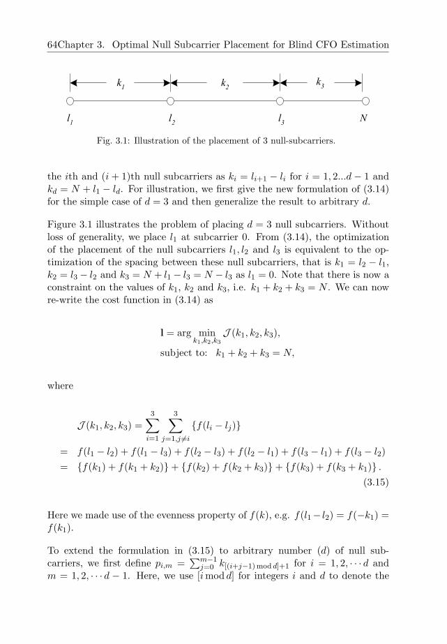
64Chapter 3. Optimal Null Subcarrier Placement for Blind CFO Estimation
l1
l2
l3
k1
k2
k3
N
Fig. 3.1: Illustration of the placement of 3 null-subcarriers.
the ith and (i + 1)th null subcarriers as ki = li+1 − li for i = 1, 2...d − 1 andkd = N + l1 − ld. For illustration, we first give the new formulation of (3.14)for the simple case of d = 3 and then generalize the result to arbitrary d.
Figure 3.1 illustrates the problem of placing d = 3 null subcarriers. Withoutloss of generality, we place l1 at subcarrier 0. From (3.14), the optimizationof the placement of the null subcarriers l1, l2 and l3 is equivalent to the op-timization of the spacing between these null subcarriers, that is k1 = l2 − l1,k2 = l3 − l2 and k3 = N + l1 − l3 = N − l3 as l1 = 0. Note that there is now aconstraint on the values of k1, k2 and k3, i.e. k1 + k2 + k3 = N . We can nowre-write the cost function in (3.14) as
l = arg mink1,k2,k3
J (k1, k2, k3),
subject to: k1 + k2 + k3 = N,
where
J (k1, k2, k3) =3∑
i=1
3∑
j=1,j 6=i
f(li − lj)
= f(l1 − l2) + f(l1 − l3) + f(l2 − l3) + f(l2 − l1) + f(l3 − l1) + f(l3 − l2)= f(k1) + f(k1 + k2)+ f(k2) + f(k2 + k3)+ f(k3) + f(k3 + k1) .
(3.15)
Here we made use of the evenness property of f(k), e.g. f(l1− l2) = f(−k1) =f(k1).
To extend the formulation in (3.15) to arbitrary number (d) of null sub-carriers, we first define pi,m =
∑m−1j=0 k[(i+j−1)mod d]+1 for i = 1, 2, · · · d and
m = 1, 2, · · · d − 1. Here, we use [i mod d] for integers i and d to denote the
3.2 Placement of Null Subcarriers Based on SNRCFO Maximization 65
integer remainder of i/d. The subscript i indicates the k index of the firstterm in the summation, because [(i + 0 − 1)mod d] + 1 = i. The subscriptm indicates the total number of terms in the summation. Therefore, pi,m isactually the spacing between the ith null-subcarrier and its mth neighbouringnull subcarrier to the right in the cyclic sense1. Therefore, the contribution tothe total cost function due to a particular null subcarrier i is the summation off(li−lj) from all its d−1 neighbouring null subcarriers, i.e.
∑dj=1,j 6=i f(li−lj).
As pi,m is the spacing between the ith null subcarrier and its mth neighbouringnull subcarrier, we can write
∑dj=1,j 6=i f(li − lj) =
∑d−1m=1 f(pi,m). Summing
this over all the d null subcarriers, i.e. d possible values of i, the new costfunction can be written as
J (k1, k2, · · · , kd) =d∑
i=1
d−1∑
m=1
f(pi,m) =d−1∑
m=1
d∑
i=1
f(pi,m)
subject to:d∑
i=1
ki = N. (3.16)
Notice that the optimization problem in (3.16) has all variables being positiveintegers. Such an integer programming problem is difficult to solve analyti-cally. Therefore, we first relax the constraints on all ki’s being positive integersand assume them to be positive real numbers. This approach has been com-monly used in finding the optimal bit allocations for multiuser or multicarriersystems, see for example [76]. For ease of analysis, we also assume that θ < 1so that k − θ > 0 and k + θ < N are satisfied for all possible values of k. Itcan be easily shown that if θ < 1 is satisfied, the double derivative of f(k)with respect to k, d2
dk2 f(k) > 0 for 1 < k < N − 1. Therefore, f(k) is a convexfunction for 1 < k < N −1 and θ < 1. It is stated in [77] that if f(k) is convexfor k1, k2, · · · , kd, and given λ1, λ2, · · · , λd with λ1 + λ2 + · · ·+ λd = 1, then
f(λ1k1 + λ2k2 + · · ·+ λdkd) ≤ λ1f(k1) + λ2f(k2) + · · ·+ λdf(kd). (3.17)
This relationship is also known as the Jensen inequality. By setting λ1 = λ2 =
1The length of the cycle is d as there are only d null subcarriers.
66Chapter 3. Optimal Null Subcarrier Placement for Blind CFO Estimation
· · · = λd = 1d , we have
1d
d∑
i=1
f(pi,m) ≥ f
(1d
d∑
i=1
pi,m
)= f
(mN
d
)for m = 1, 2, · · · d− 1. (3.18)
Here we make use of the fact that∑d
i=1 pi,m = mN because∑d
i=1 ki = N .When k1 = k2 = · · · = kd = N
d , the equality in (3.18) holds for all the valuesof m. Therefore, we get
J (k1, k2, · · · , kd) =d−1∑
m=1
d∑
i=1
f(pi,m)
≥
d−1∑
m=1
d
f
(mN
d
). (3.19)
This cost function is minimized when k1 = k2 = · · · = kd = Nd . This means
that the null subcarriers should be placed evenly-spaced across the wholeOFDM symbol.
If Nd is an integer, the null subcarriers should be placed N
d apart to maximizeSNRCFO. Therefore, in system design when we can freely choose the numberof null subcarriers d, we should always choose d such that N
d is an integerto ensure the optimality of null subcarrier placement. However, for systemswhere N is not divisible by d, it turns out difficult to prove the optimality of aparticular null subcarrier placement because of the integer constraints on thevalues of ki’s. However, from the optimal solution for real ki, we know that tomaximize the SNRCFO, the spacing between the null subcarriers should be aseven as possible. In the following, we propose a heuristic procedure to achievethis.
Let kl = bNd c and ku = dN
d e where kl and ku are both integers. Here we usebxc to denote the largest integer that is smaller than or equal to x, while dxedenotes the smallest integer that is larger than or equal to x. We know thatto achieve close to even spacing between the null subcarriers, all the ki valuesshould be chosen as either kl or ku. Next we determine how many ki’s shouldtake the value kl and how many ki’s should take the value ku and we use nl
and nu to denote these two numbers respectively. The values of nl and nu can
3.2 Placement of Null Subcarriers Based on SNRCFO Maximization 67
be obtained by solving
nl + nu = dnl × kl + nu × ku = N.
Now the problem of placing the null subcarriers is equivalent to placing thesenl kl’s and nu ku’s as evenly as possible. It is obvious that if we place all thekl’s consecutively and all the ku’s consecutively, the spacing between the nullsubcarriers will not be very even. They should be placed alternately in someway. Without loss of generality, let us assume nl ≥ nu. If nl
nu= q is an integer,
we should group q kl’s followed by one ku into one group and place nu of suchgroups as illustrated in Table 3.1. Otherwise, we let ql = b nl
nuc. In this case,
we should have two kinds of placing groups. The type 1 group consists of ql
kl’s followed by one ku and the type 2 group consists of ql + 1 kl’s followed byone ku. The number of type 1 groups gl and number of type 2 groups gu canbe obtained by solving
gl + gu = nu
gl × ql + gu × (ql + 1) = nl.
These two types of groups should be placed alternately. A summary of thisheuristic placement method is given in Table 3.1.
Let us illustrate this procedure with an example. Suppose we want to place10 null subcarriers for an OFDM system with N = 64 subcarriers. We firstcalculate kl = b64
10c = 6 and ku = d6410e = 7. We can also get nl = 6, nu = 4.
Now we need to place these 6 kl’s and 4 k′us as evenly as possible. Next wedetermine ql = b1.5c = 1, gl = 2 and gu = 2. In this case, the ki’s should bedivided into two types of groups. The type one group consists of one (ql) kl
followed by one ku, while the type 2 group consists of two (ql+1) kl followed byone ku. And these two types of groups should be placed alternately. Therefore,the spacing between the null subcarriers should be [6 7 6 6 7 6 7 6 6 7]. Hence,one possible null subcarrier placement using this heuristic approach is [0 6 1319 25 32 38 45 51 57].2
The null subcarrier placement for d = 4 to d = 11 null subcarriers for an
2Because the positions of the null subcarriers can be cyclically shifted without affectingthe value of the cost function, there are multiple solutions to the null subcarrier placement.What we have here is just one possible placement.
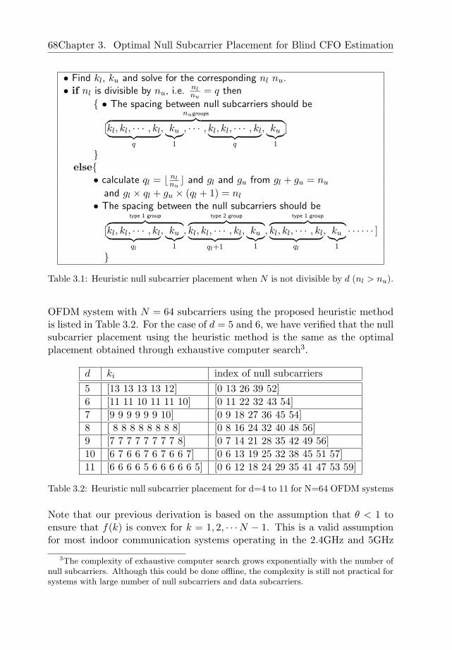
68Chapter 3. Optimal Null Subcarrier Placement for Blind CFO Estimation
• Find kl, ku and solve for the corresponding nl nu.• if nl is divisible by nu, i.e. nl
nu= q then
• The spacing between null subcarriers should be
[
nugroups︷ ︸︸ ︷kl, kl, · · · , kl︸ ︷︷ ︸
q
, ku︸︷︷︸1
, · · · , kl, kl, · · · , kl︸ ︷︷ ︸q
, ku︸︷︷︸1
]
else
• calculate ql = b nlnuc and gl and gu from gl + gu = nu
and gl × ql + gu × (ql + 1) = nl
• The spacing between the null subcarriers should be
[
type 1 group︷ ︸︸ ︷kl, kl, · · · , kl︸ ︷︷ ︸
ql
, ku︸︷︷︸1
,
type 2 group︷ ︸︸ ︷kl, kl, · · · , kl︸ ︷︷ ︸
ql+1
, ku︸︷︷︸1
,
type 1 group︷ ︸︸ ︷kl, kl, · · · , kl︸ ︷︷ ︸
ql
, ku︸︷︷︸1
· · · · · · ]
Table 3.1: Heuristic null subcarrier placement when N is not divisible by d (nl > nu).
OFDM system with N = 64 subcarriers using the proposed heuristic methodis listed in Table 3.2. For the case of d = 5 and 6, we have verified that the nullsubcarrier placement using the heuristic method is the same as the optimalplacement obtained through exhaustive computer search3.
d ki index of null subcarriers5 [13 13 13 13 12] [0 13 26 39 52]6 [11 11 10 11 11 10] [0 11 22 32 43 54]7 [9 9 9 9 9 9 10] [0 9 18 27 36 45 54]8 [ 8 8 8 8 8 8 8 8] [0 8 16 24 32 40 48 56]9 [7 7 7 7 7 7 7 7 8] [0 7 14 21 28 35 42 49 56]10 [6 7 6 6 7 6 7 6 6 7] [0 6 13 19 25 32 38 45 51 57]11 [6 6 6 6 5 6 6 6 6 6 5] [0 6 12 18 24 29 35 41 47 53 59]
Table 3.2: Heuristic null subcarrier placement for d=4 to 11 for N=64 OFDM systems
Note that our previous derivation is based on the assumption that θ < 1 toensure that f(k) is convex for k = 1, 2, · · ·N − 1. This is a valid assumptionfor most indoor communication systems operating in the 2.4GHz and 5GHz
3The complexity of exhaustive computer search grows exponentially with the number ofnull subcarriers. Although this could be done offline, the complexity is still not practical forsystems with large number of null subcarriers and data subcarriers.
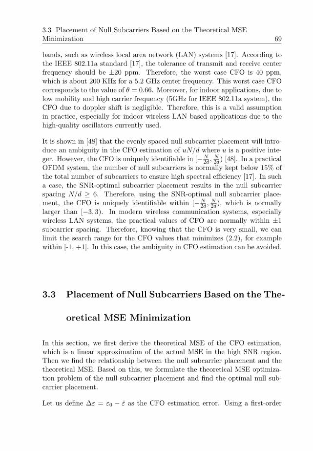
3.3 Placement of Null Subcarriers Based on the Theoretical MSEMinimization 69
bands, such as wireless local area network (LAN) systems [17]. According tothe IEEE 802.11a standard [17], the tolerance of transmit and receive centerfrequency should be ±20 ppm. Therefore, the worst case CFO is 40 ppm,which is about 200 KHz for a 5.2 GHz center frequency. This worst case CFOcorresponds to the value of θ = 0.66. Moreover, for indoor applications, due tolow mobility and high carrier frequency (5GHz for IEEE 802.11a system), theCFO due to doppler shift is negligible. Therefore, this is a valid assumptionin practice, especially for indoor wireless LAN based applications due to thehigh-quality oscillators currently used.
It is shown in [48] that the evenly spaced null subcarrier placement will intro-duce an ambiguity in the CFO estimation of uN/d where u is a positive inte-ger. However, the CFO is uniquely identifiable in [−N
2d , N2d) [48]. In a practical
OFDM system, the number of null subcarriers is normally kept below 15% ofthe total number of subcarriers to ensure high spectral efficiency [17]. In sucha case, the SNR-optimal subcarrier placement results in the null subcarrierspacing N/d ≥ 6. Therefore, using the SNR-optimal null subcarrier place-ment, the CFO is uniquely identifiable within [−N
2d , N2d), which is normally
larger than [−3, 3). In modern wireless communication systems, especiallywireless LAN systems, the practical values of CFO are normally within ±1subcarrier spacing. Therefore, knowing that the CFO is very small, we canlimit the search range for the CFO values that minimizes (2.2), for examplewithin [-1, +1]. In this case, the ambiguity in CFO estimation can be avoided.
3.3 Placement of Null Subcarriers Based on the The-
oretical MSE Minimization
In this section, we first derive the theoretical MSE of the CFO estimation,which is a linear approximation of the actual MSE in the high SNR region.Then we find the relationship between the null subcarrier placement and thetheoretical MSE. Based on this, we formulate the theoretical MSE optimiza-tion problem of the null subcarrier placement and find the optimal null sub-carrier placement.
Let us define ∆ε = ε0 − ε as the CFO estimation error. Using a first-order
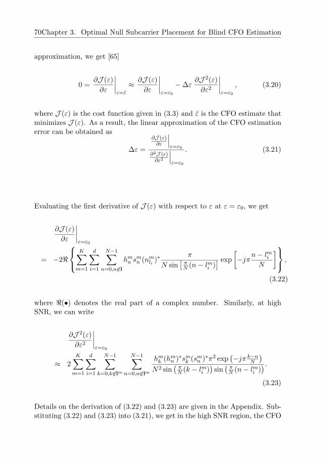
70Chapter 3. Optimal Null Subcarrier Placement for Blind CFO Estimation
approximation, we get [65]
0 =∂J (ε)
∂ε
∣∣∣∣ε=ε
≈ ∂J (ε)∂ε
∣∣∣∣ε=ε0
−∆ε∂J 2(ε)
∂ε2
∣∣∣∣ε=ε0
, (3.20)
where J (ε) is the cost function given in (3.3) and ε is the CFO estimate thatminimizes J (ε). As a result, the linear approximation of the CFO estimationerror can be obtained as
∆ε =
∂J (ε)∂ε
∣∣∣ε=ε0
∂2J (ε)∂ε2
∣∣∣ε=ε0
. (3.21)
Evaluating the first derivative of J (ε) with respect to ε at ε = ε0, we get
∂J (ε)∂ε
∣∣∣∣ε=ε0
= −2<
K∑
m=1
d∑
i=1
N−1∑
n=0,n6∈l
hmn sm
n (nmli
)∗π
N sin[
πN (n− lmi )
] exp[−jπ
n− lmiN
] ,
(3.22)
where <(•) denotes the real part of a complex number. Similarly, at highSNR, we can write
∂J 2(ε)∂ε2
∣∣∣∣ε=ε0
≈ 2K∑
m=1
d∑
i=1
N−1∑
k=0,k 6∈lm
N−1∑
n=0,n6∈lm
hmk (hm
n )∗smk (sm
n )∗π2 exp(−jπ k−n
N
)
N2 sin(
πN (k − lmi )
)sin
(πN (n− lmi )
) .
(3.23)
Details on the derivation of (3.22) and (3.23) are given in the Appendix. Sub-stituting (3.22) and (3.23) into (3.21), we get in the high SNR region, the CFO
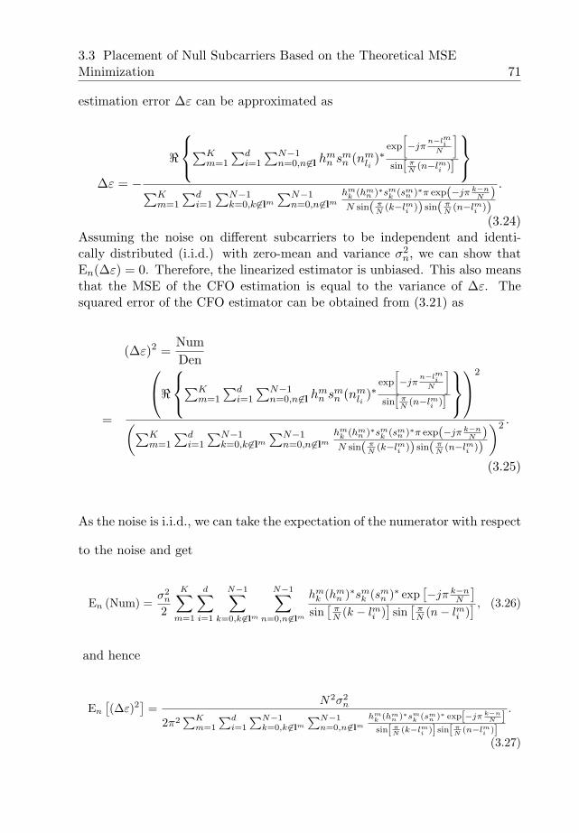
3.3 Placement of Null Subcarriers Based on the Theoretical MSEMinimization 71
estimation error ∆ε can be approximated as
∆ε = −<
∑Km=1
∑di=1
∑N−1n=0,n6∈l h
mn sm
n (nmli
)∗exp
[−jπ
n−lmiN
]
sin[ πN
(n−lmi )]
∑Km=1
∑di=1
∑N−1k=0,k 6∈lm
∑N−1n=0,n6∈lm
hmk (hm
n )∗smk (sm
n )∗π exp(−jπ k−nN )
N sin( πN
(k−lmi )) sin( πN
(n−lmi ))
.
(3.24)Assuming the noise on different subcarriers to be independent and identi-cally distributed (i.i.d.) with zero-mean and variance σ2
n, we can show thatEn(∆ε) = 0. Therefore, the linearized estimator is unbiased. This also meansthat the MSE of the CFO estimation is equal to the variance of ∆ε. Thesquared error of the CFO estimator can be obtained from (3.21) as
(∆ε)2 =NumDen
=
<
∑Km=1
∑di=1
∑N−1n=0,n6∈l h
mn sm
n (nmli
)∗exp
[−jπ
n−lmiN
]
sin[ πN
(n−lmi )]
2
(∑Km=1
∑di=1
∑N−1k=0,k 6∈lm
∑N−1n=0,n6∈lm
hmk (hm
n )∗smk (sm
n )∗π exp(−jπ k−nN )
N sin( πN
(k−lmi )) sin( πN
(n−lmi ))
)2 .
(3.25)
As the noise is i.i.d., we can take the expectation of the numerator with respect
to the noise and get
En (Num) =σ2
n
2
K∑m=1
d∑
i=1
N−1∑
k=0,k 6∈lm
N−1∑
n=0,n 6∈lm
hmk (hm
n )∗smk (sm
n )∗ exp[−jπ k−n
N
]
sin[
πN (k − lmi )
]sin
[πN (n− lmi )
] , (3.26)
and hence
En
[(∆ε)2
]=
N2σ2n
2π2∑K
m=1
∑di=1
∑N−1k=0,k 6∈lm
∑N−1n=0,n 6∈lm
hmk (hm
n )∗smk (sm
n )∗ exp[−jπ k−nN ]
sin[ πN (k−lmi )] sin[ π
N (n−lmi )]
.
(3.27)
72Chapter 3. Optimal Null Subcarrier Placement for Blind CFO Estimation
Let us assume that the transmitted signal smk is i.i.d. with zero-mean and
unit-variance, i.e. E[smk (sm
n )∗] = δ(k − n), where δ(•) denotes the dirac deltafunction. Averaging En
[(∆ε)2
]over transmitted signal leads us to
Lemma 1: In the high SNR region, the theoretical MSE of the CFO estimationfor a realization of a multipath channel h for K OFDM symbols is
MSE(ε|h) = En,s
[(∆ε)2|h]
=N2σ2
n
2π2∑K
m=1
∑di=1
∑N−1n=0,n6∈lm |hm
n |2 1sin2[ π
N(n−lmi )]
.
(3.28)Now we average the theoretical MSE over different realizations of channel h.Similar as before, we assume that channel response on each subcarrier is zero-mean with unit variance, i.e. E(hm
n )=0 and E(|hmn |2)=1 for n = 0, 1, · · · , N−1
and m = 1, · · · ,K, we get the following result:
Lemma 2: In the high SNR region, the theoretical MSE of the CFO estimationis
MSE(ε) = En,s,h
[(∆ε)2
]=
N2σ2n
2π2∑K
m=1
∑di=1
∑N−1n=0,n6∈lm
1sin2[ π
N(n−lmi )]
. (3.29)
Now, let us look at the null subcarrier optimization problem again. The nullsubcarrier placement that minimizes the theoretical MSE can be formulatedas
l = arg minl
(MSE) = arg maxl
K∑
m=1
d∑
i=1
N−1∑
n=0,n6∈lm
1sin2
[πN (n− lmi )
] . (3.30)
If∑d
i=1
∑N−1n=0,n6∈lm
1sin2[ π
N(n−lmi )] is maximized for every value of m, i.e. for each
OFDM symbol, then the cost function in (3.30) is maximized. Therefore, theoptimization problem over K OFDM symbols is equivalent to the optimization
3.4 Practical Considerations 73
in one OFDM symbol given by
l = arg minl
(MSE) = arg maxl
d∑
i=1
N−1∑
n=0,n6∈l
1sin2
[πN (n− li)
]
= arg maxl
d∑
i=1
N−1∑
n=0,n6∈l
g(n− li)
, (3.31)
where g(k) = 1sin2[ π
N(n−li)] . It is straight-forward to show that g(k) is also
periodic with period of N . Using a similar approach as in Section 3.2, the costfunction in (3.31) can be simplified to
l = arg maxl
c1 −
d∑
i=1
∑
n∈l,n6=li
g(n− li)
= arg minl
d∑
i=1
d∑
j=1,j 6=i
g(li − lj)
. (3.32)
It can also be shown that g(x) is a convex function of real number x for1 < x < N − 1. Therefore, the cost function in (3.32) is essentially of thesame form as the cost function in (3.14) as g(x) and f(x) are both convex.This means the optimal null subcarrier placement l that minimize both costfunctions are the same. Thus we have proven
Proposition: The null subcarrier placement that maximizes the SNR of CFOestimation defined in (3.5) also minimizes the theoretical MSE of the CFOestimation given in (3.29).
3.4 Practical Considerations
For practical OFDM systems, it is usually necessary to place some null sub-carriers consecutively at both ends of the spectrum as guard bands. We callthese null subcarriers the guard null subcarriers. In this section, we show
74Chapter 3. Optimal Null Subcarrier Placement for Blind CFO Estimation
that given the fixed positions of the guard null subcarriers, if there are a fewnull subcarriers to place freely in the OFDM symbol for the purpose of CFOestimation, which we call free null subcarriers, how we should place them tomaximize SNRCFO.
Figure 1.12 illustrates an OFDM system having two guard bands with d1
and d2 null subcarriers respectively. Here, we have re-arranged the OFDMsubcarrier index from −N/2 + 1 to N/2 such that the purpose of the guardbands is more obvious. However, such re-arrangement does not affect theformulation of the cost function due to the circular symmetry of the OFDMsystem. Suppose that we have dn free null subcarriers that we can place freelybetween subcarrier −N/2 + d1 and N/2− d2 + 1, the whole set of all the nullsubcarriers becomes
l = [l1, l2, · · · , ld1 , ld1+1, · · · , ld1+dn , ld1+dn+1, · · · , ld],
where d = d1 + d2 + dn is the total number of null subcarriers. Again wedefine ki = li+1 − li as the spacing between the li+1th null subcarrier and thelth null subcarrier and pi,m =
∑m−1j=0 k[(i+j−1) mod d]+1 as the spacing between
the ith null-subcarrier and its mth neighbouring null subcarrier to the right inthe cyclic sense. Notice that given the positions of the guard null subcarriersfixed at both ends of the spectrum, the positions of the free null subcarriersare uniquely determined by the following quantities:
• The spacing kd1 between the left most free null subcarrier ld1+1 and theright most guard null subcarrier in the left guard band ld1 ,
• The spacing kd1+dn between the right most free null subcarrier ld1+dn andthe left most guard null subcarrier in the right guard band ld1+dn+1,
• The spacing kd1+1 · · · kd1+dn−1 between the free null subcarriers.
Following a similar procedure as in Section 3.2, we obtain the cost function ofnull subcarrier placement for an OFDM system with guard band as
J (kd1 , kd1+1, · · · , kd1+dn) =d∑
i=1
d−1∑
m=1
f(pi,m)
subject to:d∑
i=1
ki = N. (3.33)
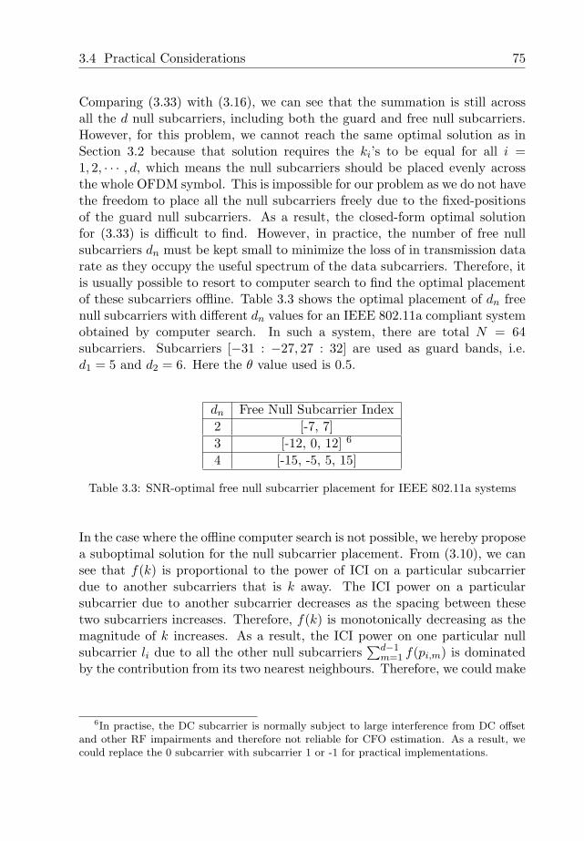
3.4 Practical Considerations 75
Comparing (3.33) with (3.16), we can see that the summation is still acrossall the d null subcarriers, including both the guard and free null subcarriers.However, for this problem, we cannot reach the same optimal solution as inSection 3.2 because that solution requires the ki’s to be equal for all i =1, 2, · · · , d, which means the null subcarriers should be placed evenly acrossthe whole OFDM symbol. This is impossible for our problem as we do not havethe freedom to place all the null subcarriers freely due to the fixed-positionsof the guard null subcarriers. As a result, the closed-form optimal solutionfor (3.33) is difficult to find. However, in practice, the number of free nullsubcarriers dn must be kept small to minimize the loss of in transmission datarate as they occupy the useful spectrum of the data subcarriers. Therefore, itis usually possible to resort to computer search to find the optimal placementof these subcarriers offline. Table 3.3 shows the optimal placement of dn freenull subcarriers with different dn values for an IEEE 802.11a compliant systemobtained by computer search. In such a system, there are total N = 64subcarriers. Subcarriers [−31 : −27, 27 : 32] are used as guard bands, i.e.d1 = 5 and d2 = 6. Here the θ value used is 0.5.
dn Free Null Subcarrier Index2 [-7, 7]3 [-12, 0, 12] 6
4 [-15, -5, 5, 15]
Table 3.3: SNR-optimal free null subcarrier placement for IEEE 802.11a systems
In the case where the offline computer search is not possible, we hereby proposea suboptimal solution for the null subcarrier placement. From (3.10), we cansee that f(k) is proportional to the power of ICI on a particular subcarrierdue to another subcarriers that is k away. The ICI power on a particularsubcarrier due to another subcarrier decreases as the spacing between thesetwo subcarriers increases. Therefore, f(k) is monotonically decreasing as themagnitude of k increases. As a result, the ICI power on one particular nullsubcarrier li due to all the other null subcarriers
∑d−1m=1 f(pi,m) is dominated
by the contribution from its two nearest neighbours. Therefore, we could make
6In practise, the DC subcarrier is normally subject to large interference from DC offsetand other RF impairments and therefore not reliable for CFO estimation. As a result, wecould replace the 0 subcarrier with subcarrier 1 or -1 for practical implementations.
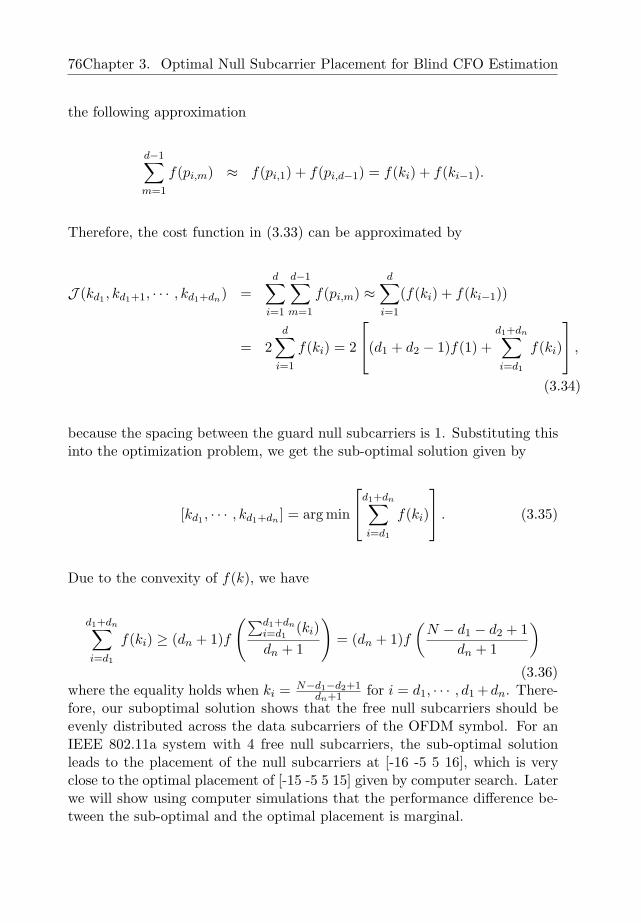
76Chapter 3. Optimal Null Subcarrier Placement for Blind CFO Estimation
the following approximation
d−1∑
m=1
f(pi,m) ≈ f(pi,1) + f(pi,d−1) = f(ki) + f(ki−1).
Therefore, the cost function in (3.33) can be approximated by
J (kd1 , kd1+1, · · · , kd1+dn) =d∑
i=1
d−1∑
m=1
f(pi,m) ≈d∑
i=1
(f(ki) + f(ki−1))
= 2d∑
i=1
f(ki) = 2
(d1 + d2 − 1)f(1) +
d1+dn∑
i=d1
f(ki)
,
(3.34)
because the spacing between the guard null subcarriers is 1. Substituting thisinto the optimization problem, we get the sub-optimal solution given by
[kd1 , · · · , kd1+dn ] = arg min
d1+dn∑
i=d1
f(ki)
. (3.35)
Due to the convexity of f(k), we have
d1+dn∑
i=d1
f(ki) ≥ (dn + 1)f
(∑d1+dni=d1
(ki)dn + 1
)= (dn + 1)f
(N − d1 − d2 + 1
dn + 1
)
(3.36)where the equality holds when ki = N−d1−d2+1
dn+1 for i = d1, · · · , d1 +dn. There-fore, our suboptimal solution shows that the free null subcarriers should beevenly distributed across the data subcarriers of the OFDM symbol. For anIEEE 802.11a system with 4 free null subcarriers, the sub-optimal solutionleads to the placement of the null subcarriers at [-16 -5 5 16], which is veryclose to the optimal placement of [-15 -5 5 15] given by computer search. Laterwe will show using computer simulations that the performance difference be-tween the sub-optimal and the optimal placement is marginal.
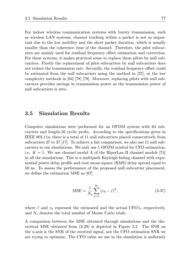
3.5 Simulation Results 77
For indoor wireless communication systems with bursty transmission, suchas wireless LAN systems, channel tracking within a packet is not so impor-tant due to the low mobility and the short packet duration, which is usuallysmaller than the coherence time of the channel. Therefore, the pilot subcar-riers are mainly used for residual frequency offset estimation and correction.For these systems, it makes practical sense to replace these pilots by null sub-carriers. Firstly the replacement of pilot subcarriers by null subcarriers doesnot reduce the transmission rate. Secondly, the residual frequency offset couldbe estimated from the null subcarriers using the method in [37], or the lowcomplexity methods in [64] [78] [79]. Moreover, replacing pilots with null sub-carriers provides savings in transmission power as the transmission power ofnull subcarriers is zero.
3.5 Simulation Results
Computer simulations were performed for an OFDM system with 64 sub-carriers and length-16 cyclic prefix. According to the specifications given inIEEE 802.11a, there is a total of 11 null subcarriers placed consecutively fromsubcarriers 27 to 37 [17]. To achieve a fair comparison, we also use 11 null sub-carriers in our simulations. We only use 1 OFDM symbol for CFO estimation,i.e. K = 1. We use channel model A of the HiperLan II channel models [74]in all the simulations. This is a multipath Rayleigh fading channel with expo-nential power delay profile and root mean square (RMS) delay spread equal to50 ns. To assess the performance of the proposed null subcarrier placement,we define the estimation MSE as [67]
MSE =1
Ns
Ns∑
i=1
(ε0 − ε)2 , (3.37)
where ε and ε0 represent the estimated and the actual CFO’s, respectively,and Ns denotes the total number of Monte Carlo trials.
A comparison between the MSE obtained through simulations and the the-oretical MSE obtained from (3.29) is depicted in Figure 3.2. The SNR onthe x-axis is the SNR of the received signal, not the CFO estimation SNR weare trying to optimize. The CFO value we use in the simulation is uniformly
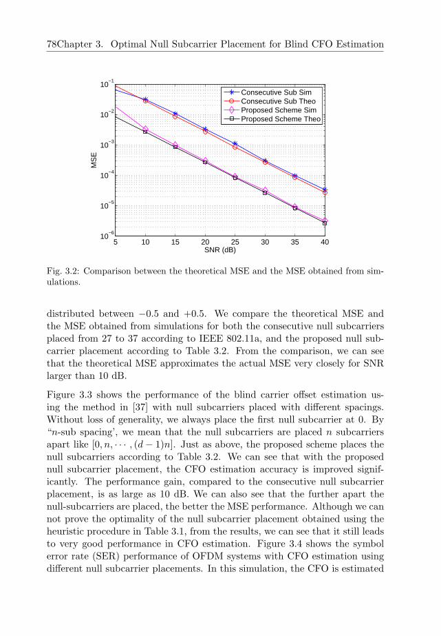
78Chapter 3. Optimal Null Subcarrier Placement for Blind CFO Estimation
5 10 15 20 25 30 35 4010
−6
10−5
10−4
10−3
10−2
10−1
SNR (dB)
MS
E
Consecutive Sub SimConsecutive Sub TheoProposed Scheme SimProposed Scheme Theo
Fig. 3.2: Comparison between the theoretical MSE and the MSE obtained from sim-ulations.
distributed between −0.5 and +0.5. We compare the theoretical MSE andthe MSE obtained from simulations for both the consecutive null subcarriersplaced from 27 to 37 according to IEEE 802.11a, and the proposed null sub-carrier placement according to Table 3.2. From the comparison, we can seethat the theoretical MSE approximates the actual MSE very closely for SNRlarger than 10 dB.
Figure 3.3 shows the performance of the blind carrier offset estimation us-ing the method in [37] with null subcarriers placed with different spacings.Without loss of generality, we always place the first null subcarrier at 0. By“n-sub spacing’, we mean that the null subcarriers are placed n subcarriersapart like [0, n, · · · , (d− 1)n]. Just as above, the proposed scheme places thenull subcarriers according to Table 3.2. We can see that with the proposednull subcarrier placement, the CFO estimation accuracy is improved signif-icantly. The performance gain, compared to the consecutive null subcarrierplacement, is as large as 10 dB. We can also see that the further apart thenull-subcarriers are placed, the better the MSE performance. Although we cannot prove the optimality of the null subcarrier placement obtained using theheuristic procedure in Table 3.1, from the results, we can see that it still leadsto very good performance in CFO estimation. Figure 3.4 shows the symbolerror rate (SER) performance of OFDM systems with CFO estimation usingdifferent null subcarrier placements. In this simulation, the CFO is estimated
3.5 Simulation Results 79
5 7.5 10 12.5 15 17.5 2010
−4
10−3
10−2
10−1
SNR (dB)
MS
E
Consecutive sub2−sub spacing3−sub spacing4−sub spacingProposed Scheme
Fig. 3.3: MSE performance of the CFO estimation using different null subcarrierplacements.
using the method in [37] and compensated. We use QPSK modulation andassume perfect channel estimation. A performance gain of about 3.5 dB canbe achieved using the proposed placement compared to consecutively-placednull subcarriers.
Figure 3.5 shows the improvement in CFO estimation achieved by introducinga few optimally-placed free null subcarriers besides the guard null subcarriers.The system follows IEEE 802.11a specifications with 11 guard null subcarri-ers. The CFO value we used in the simulation is again uniformly distributedbetween −0.5 and +0.5. We can see by introducing 2 extra free null sub-carriers, the performance of the CFO estimation can be improved by 5 dBcompared to using guard null subcarriers alone. The performance can be fur-ther improved by introducing more free null subcarriers. The gain, on theother hand, becomes smaller as the number of free null subcarriers increases.We also compared the performance of using 4 free null subcarriers with theoptimal placement by computer search and the sub-optimal placement by us-ing the approximated cost function. The results show that the performancedifference between these two placement is rather marginal.
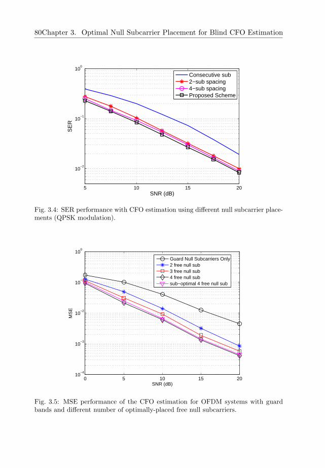
80Chapter 3. Optimal Null Subcarrier Placement for Blind CFO Estimation
5 10 15 20
10−2
10−1
100
SNR (dB)
SE
R
Consecutive sub2−sub spacing4−sub spacingProposed Scheme
Fig. 3.4: SER performance with CFO estimation using different null subcarrier place-ments (QPSK modulation).
0 5 10 15 2010
−4
10−3
10−2
10−1
100
SNR (dB)
MS
E
Guard Null Subcarriers Only2 free null sub3 free null sub4 free null subsub−optimal 4 free null sub
Fig. 3.5: MSE performance of the CFO estimation for OFDM systems with guardbands and different number of optimally-placed free null subcarriers.
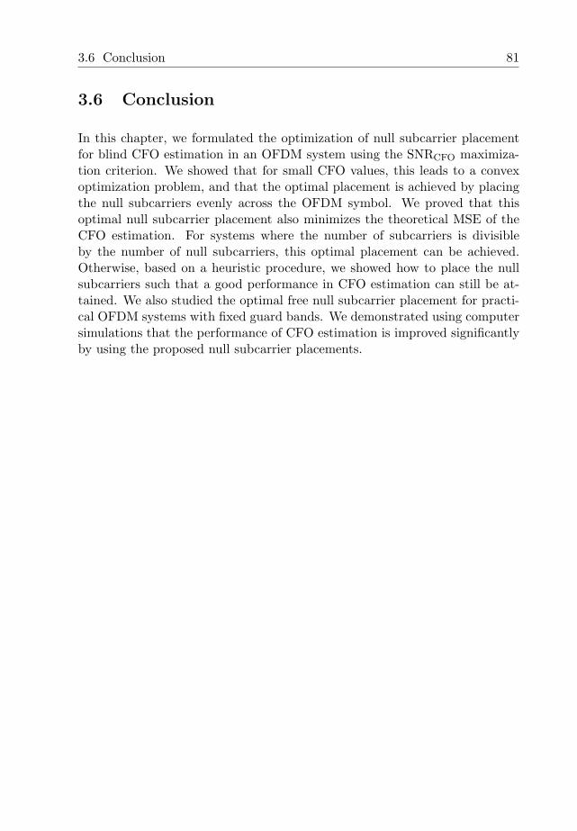
3.6 Conclusion 81
3.6 Conclusion
In this chapter, we formulated the optimization of null subcarrier placementfor blind CFO estimation in an OFDM system using the SNRCFO maximiza-tion criterion. We showed that for small CFO values, this leads to a convexoptimization problem, and that the optimal placement is achieved by placingthe null subcarriers evenly across the OFDM symbol. We proved that thisoptimal null subcarrier placement also minimizes the theoretical MSE of theCFO estimation. For systems where the number of subcarriers is divisibleby the number of null subcarriers, this optimal placement can be achieved.Otherwise, based on a heuristic procedure, we showed how to place the nullsubcarriers such that a good performance in CFO estimation can still be at-tained. We also studied the optimal free null subcarrier placement for practi-cal OFDM systems with fixed guard bands. We demonstrated using computersimulations that the performance of CFO estimation is improved significantlyby using the proposed null subcarrier placements.
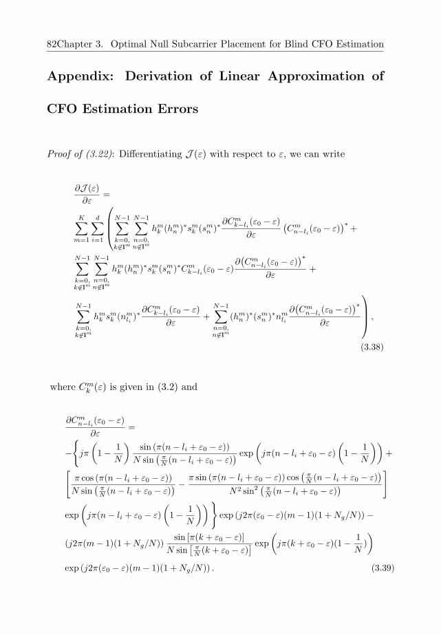
82Chapter 3. Optimal Null Subcarrier Placement for Blind CFO Estimation
Appendix: Derivation of Linear Approximation of
CFO Estimation Errors
Proof of (3.22): Differentiating J (ε) with respect to ε, we can write
∂J (ε)∂ε
=
K∑m=1
d∑
i=1
N−1∑
k=0,k 6∈lm
N−1∑n=0,n6∈lm
hmk (hm
n )∗smk (sm
n )∗∂Cm
k−li(ε0 − ε)∂ε
(Cm
n−li(ε0 − ε))∗+
N−1∑
k=0,k 6∈lm
N−1∑n=0,n 6∈lm
hmk (hm
n )∗smk (sm
n )∗Cmk−li(ε0 − ε)
∂(Cm
n−li(ε0 − ε)
)∗∂ε
+
N−1∑
k=0,k 6∈lm
hmk sm
k (nmli )∗
∂Cmk−li
(ε0 − ε)∂ε
+N−1∑n=0,n6∈lm
(hmn )∗(sm
n )∗nmli
∂(Cm
n−li(ε0 − ε)
)∗∂ε
,
(3.38)
where Cmk (ε) is given in (3.2) and
∂Cmn−li
(ε0 − ε)∂ε
=
−
jπ
(1− 1
N
)sin (π(n− li + ε0 − ε))
N sin(
πN (n− li + ε0 − ε)
) exp(
jπ(n− li + ε0 − ε)(
1− 1N
))+
[π cos (π(n− li + ε0 − ε))
N sin(
πN (n− li + ε0 − ε)
) − π sin (π(n− li + ε0 − ε)) cos(
πN (n− li + ε0 − ε)
)
N2 sin2(
πN (n− li + ε0 − ε)
)]
exp(
jπ(n− li + ε0 − ε)(
1− 1N
))exp (j2π(ε0 − ε)(m− 1)(1 + Ng/N))−
(j2π(m− 1)(1 + Ng/N))sin [π(k + ε0 − ε)]
N sin[
πN (k + ε0 − ε)
] exp(
jπ(k + ε0 − ε)(1− 1N
))
exp (j2π(ε0 − ε)(m− 1)(1 + Ng/N)) . (3.39)
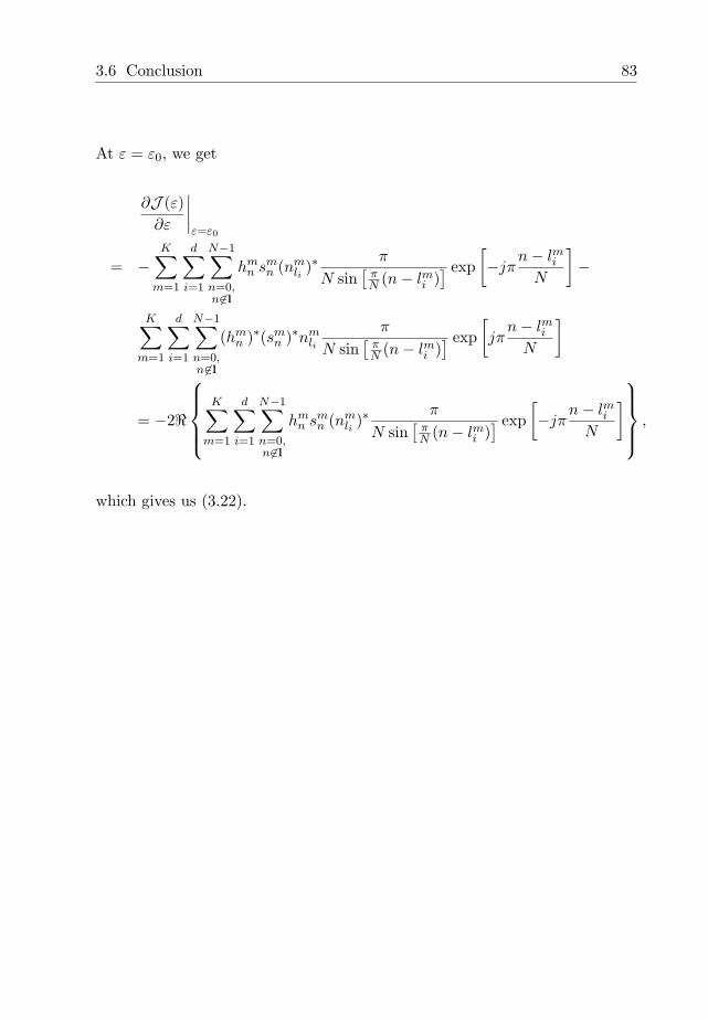
3.6 Conclusion 83
At ε = ε0, we get
∂J (ε)∂ε
∣∣∣∣ε=ε0
= −K∑
m=1
d∑
i=1
N−1∑
n=0,n 6∈l
hmn sm
n (nmli
)∗π
N sin[
πN (n− lmi )
] exp[−jπ
n− lmiN
]−
K∑
m=1
d∑
i=1
N−1∑
n=0,n 6∈l
(hmn )∗(sm
n )∗nmli
π
N sin[
πN (n− lmi )
] exp[jπ
n− lmiN
]
= −2<
K∑
m=1
d∑
i=1
N−1∑
n=0,n 6∈l
hmn sm
n (nmli
)∗π
N sin[
πN (n− lmi )
] exp[−jπ
n− lmiN
]
,
which gives us (3.22).
84Chapter 3. Optimal Null Subcarrier Placement for Blind CFO Estimation
Proof of (3.23): Differentiating (3.38) one more time, we obtain
∂2J (ε)∂ε2
=K∑
m=1
d∑
i=1
2
N−1∑
k=0,k 6∈lm
N−1∑n=0,n 6∈lm
hmk (hm
n )∗smk (sm
n )∗∂Cm
k−li(ε0 − ε)∂ε
∂(Cm
n−li(ε0 − ε)
)∗∂ε
+
N−1∑
k=0,k 6∈lm
hmk sm
k (nmli )∗
∂2Cmk−li
(ε0 − ε)∂ε2
+N−1∑n=0,n6∈l
(hmn )∗(sm
n )∗nmli
∂2(Cm
n−li(ε0 − ε)
)∗∂ε2
.
(3.40)
Similarly to [65], we can assume high SNR. i.e. |hnsn|2 À |nli |2. In this case,the second and third terms in (3.40) are much smaller than the first term andhence can be dropped in the approximation. Again at ε = ε0, we get thefollowing approximation
∂J 2(ε)∂ε2
∣∣∣∣ε=ε0
≈ 2K∑
m=1
d∑
i=1
N−1∑
k=0,k 6∈lm
N−1∑
n=0,n 6∈lm
hmk (hm
n )∗smk (sm
n )∗∂Cm
k−li(ε0 − ε)∂ε
∂(Cm
n−li(ε0 − ε)
)∗∂ε
= 2K∑
m=1
d∑
i=1
N−1∑
k=0,k 6∈lm
N−1∑
n=0,n 6∈lm
hmk (hm
n )∗smk (sm
n )∗π2 exp
(−jπ k−nN
)
N2 sin(
πN (k − lmi )
)sin
(πN (n− lmi )
) ,
(3.41)
which leads to (3.23).
Chapter 4Clock Signal Generation and
Distribution Topologies for MIMO
Systems
4.1 Introduction
It was discovered in [24] and [25] that, in rich scattering propagation envi-ronment with many reflectors and scatterers, the capacity of wireless fadingchannels is linearly proportional to the number of antennas. Since then, themultiple input and multiple output (MIMO) system, where multiple antennasare used at both the transmitter and the receiver, has received vast attentionin both academia and industry. MIMO can be used to increase the throughputof wireless systems by using spatial multiplexing techniques [80] [81]. MIMOcan also be used to reduce the system sensitivity to fading through the use ofspace-time coding techniques [29] [30]. To support these multiple antennas,
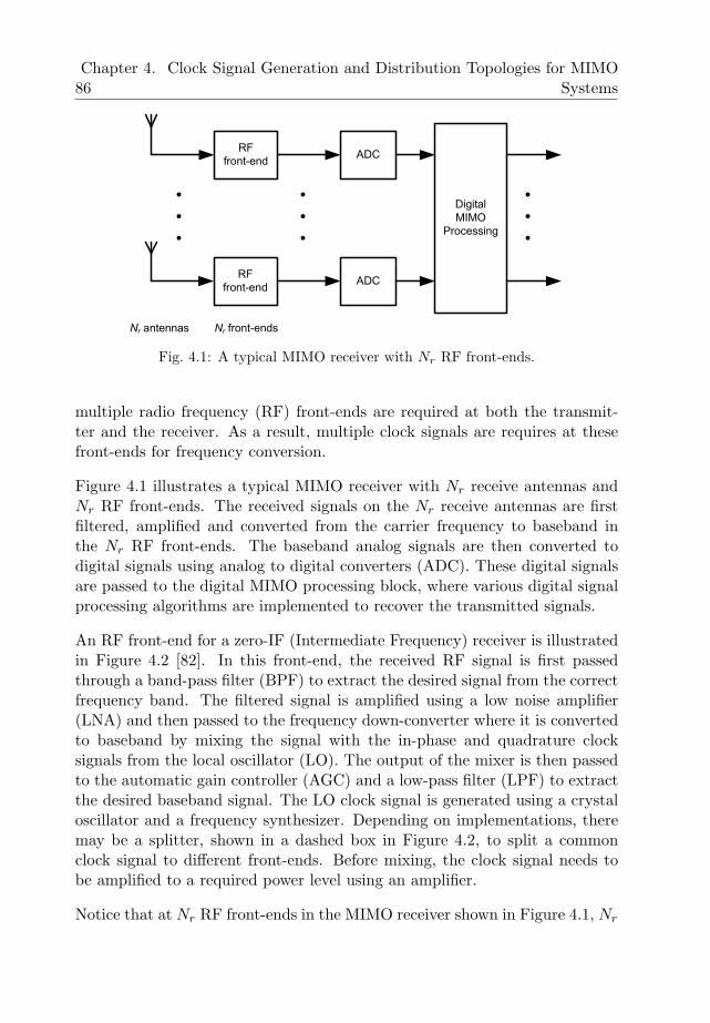
86Chapter 4. Clock Signal Generation and Distribution Topologies for MIMO
Systems
RF
front-endADC
ADC
Digital
MIMO
Processing
RF
front-end
Nr antennas Nr front-ends
Fig. 4.1: A typical MIMO receiver with Nr RF front-ends.
multiple radio frequency (RF) front-ends are required at both the transmit-ter and the receiver. As a result, multiple clock signals are requires at thesefront-ends for frequency conversion.
Figure 4.1 illustrates a typical MIMO receiver with Nr receive antennas andNr RF front-ends. The received signals on the Nr receive antennas are firstfiltered, amplified and converted from the carrier frequency to baseband inthe Nr RF front-ends. The baseband analog signals are then converted todigital signals using analog to digital converters (ADC). These digital signalsare passed to the digital MIMO processing block, where various digital signalprocessing algorithms are implemented to recover the transmitted signals.
An RF front-end for a zero-IF (Intermediate Frequency) receiver is illustratedin Figure 4.2 [82]. In this front-end, the received RF signal is first passedthrough a band-pass filter (BPF) to extract the desired signal from the correctfrequency band. The filtered signal is amplified using a low noise amplifier(LNA) and then passed to the frequency down-converter where it is convertedto baseband by mixing the signal with the in-phase and quadrature clocksignals from the local oscillator (LO). The output of the mixer is then passedto the automatic gain controller (AGC) and a low-pass filter (LPF) to extractthe desired baseband signal. The LO clock signal is generated using a crystaloscillator and a frequency synthesizer. Depending on implementations, theremay be a splitter, shown in a dashed box in Figure 4.2, to split a commonclock signal to different front-ends. Before mixing, the clock signal needs tobe amplified to a required power level using an amplifier.
Notice that at Nr RF front-ends in the MIMO receiver shown in Figure 4.1, Nr
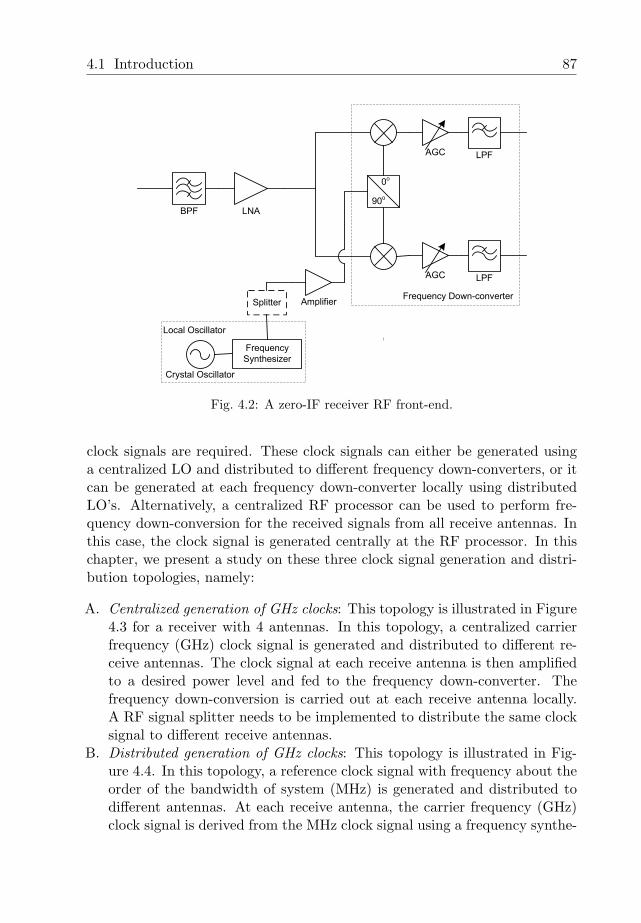
4.1 Introduction 87
LNABPF
LPF
Amplifier
AGC
LPFAGC
0o
90o
Frequency Down-converter
Crystal Oscillator
Frequency
Synthesizer
Local Oscillator
Splitter
Fig. 4.2: A zero-IF receiver RF front-end.
clock signals are required. These clock signals can either be generated usinga centralized LO and distributed to different frequency down-converters, or itcan be generated at each frequency down-converter locally using distributedLO’s. Alternatively, a centralized RF processor can be used to perform fre-quency down-conversion for the received signals from all receive antennas. Inthis case, the clock signal is generated centrally at the RF processor. In thischapter, we present a study on these three clock signal generation and distri-bution topologies, namely:
A. Centralized generation of GHz clocks: This topology is illustrated in Figure4.3 for a receiver with 4 antennas. In this topology, a centralized carrierfrequency (GHz) clock signal is generated and distributed to different re-ceive antennas. The clock signal at each receive antenna is then amplifiedto a desired power level and fed to the frequency down-converter. Thefrequency down-conversion is carried out at each receive antenna locally.A RF signal splitter needs to be implemented to distribute the same clocksignal to different receive antennas.
B. Distributed generation of GHz clocks: This topology is illustrated in Fig-ure 4.4. In this topology, a reference clock signal with frequency about theorder of the bandwidth of system (MHz) is generated and distributed todifferent antennas. At each receive antenna, the carrier frequency (GHz)clock signal is derived from the MHz clock signal using a frequency synthe-
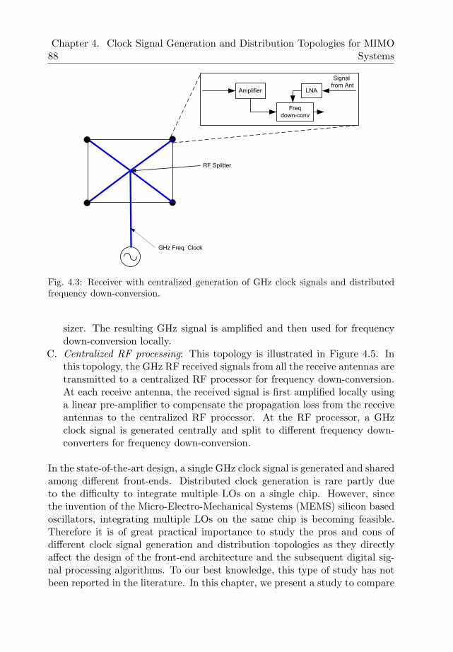
88Chapter 4. Clock Signal Generation and Distribution Topologies for MIMO
Systems
Amplifier
Freq
down-conv
LNA
Signal
from Ant
GHz Freq. Clock
RF Splitter
Fig. 4.3: Receiver with centralized generation of GHz clock signals and distributedfrequency down-conversion.
sizer. The resulting GHz signal is amplified and then used for frequencydown-conversion locally.
C. Centralized RF processing: This topology is illustrated in Figure 4.5. Inthis topology, the GHz RF received signals from all the receive antennas aretransmitted to a centralized RF processor for frequency down-conversion.At each receive antenna, the received signal is first amplified locally usinga linear pre-amplifier to compensate the propagation loss from the receiveantennas to the centralized RF processor. At the RF processor, a GHzclock signal is generated centrally and split to different frequency down-converters for frequency down-conversion.
In the state-of-the-art design, a single GHz clock signal is generated and sharedamong different front-ends. Distributed clock generation is rare partly dueto the difficulty to integrate multiple LOs on a single chip. However, sincethe invention of the Micro-Electro-Mechanical Systems (MEMS) silicon basedoscillators, integrating multiple LOs on the same chip is becoming feasible.Therefore it is of great practical importance to study the pros and cons ofdifferent clock signal generation and distribution topologies as they directlyaffect the design of the front-end architecture and the subsequent digital sig-nal processing algorithms. To our best knowledge, this type of study has notbeen reported in the literature. In this chapter, we present a study to compare
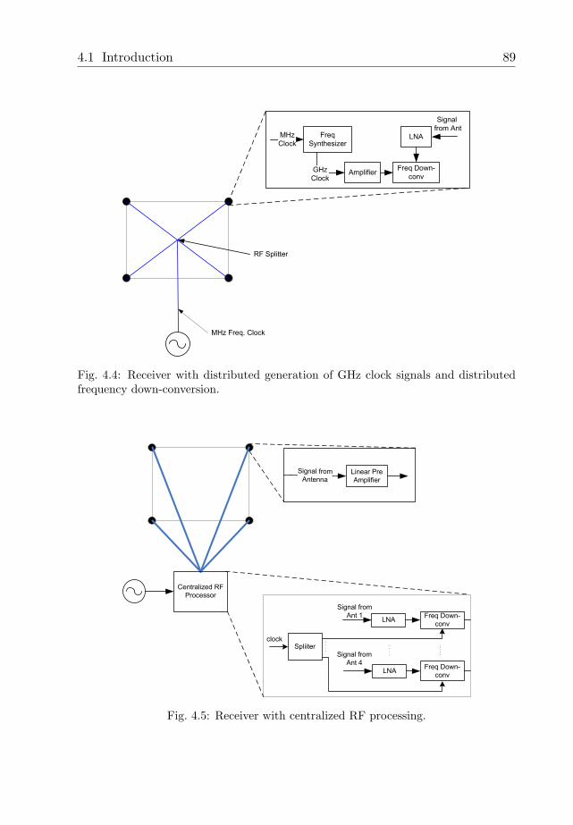
4.1 Introduction 89
MHz Freq. Clock
RF Splitter
Freq
Synthesizer
MHz
Clock
Freq Down-
convGHz
Clock
LNA
Signal
from Ant
Amplifier
Fig. 4.4: Receiver with distributed generation of GHz clock signals and distributedfrequency down-conversion.
Centralized RF
Processor
Linear Pre
Amplifier
Signal from Antenna
LNAFreq Down-
conv
Signal from
Ant 1
LNA
Signal from
Ant 4
Spliiterclock
Freq Down-
conv
Fig. 4.5: Receiver with centralized RF processing.
90Chapter 4. Clock Signal Generation and Distribution Topologies for MIMO
Systems
the above three topologies, with special emphasis on their respective powerdissipations. This is because the receiver power dissipation is becoming a ma-jor bottleneck in implementing a MIMO receiver. We first propose a generalsystem model to calculate the power dissipations for all topologies. We splitthe overall power dissipation into power dissipations at different parts of thefront-end. We then present a specific case study of the front-end power dis-sipation for a MIMO receiver with 4 receive antennas operating in three ISMbands at 2.4 GHz, 5 GHz and 60 GHz for the different clock signal gener-ation and distribution topologies. The results of the case study show thatthe frequency synthesizer dominates the total power dissipation. Therefore,to reduce power dissipation, the number of frequency synthesizers should bekept to 1. In this case, centralized clock generation is preferred. On the otherhand, the distributed topology has the big advantage that there is no carrierfrequency (GHz) RF signals traveling in the system. Compared to systemswith centralized clock topologies, where expensive materials and sophisticateddesign, such as shielding, have to be used to handle these RF signals, thedistributed clock topology allows the use of low-cost materials and simplifieddesigns.
The rest of this chapter is organized as follows. In Section 4.2, we presentthe general system model for the front-end power dissipation calculation andoutline the assumptions we used. Part of the total power dissipation of thefront-end is used to compensated the propagation loss of RF signals on mi-crostrip transmission lines in the receiver. A method to calculate this loss ispresented in Section 4.3. In Section 4.4, we present a case study on the powerdissipations of the three clock signal generation and distribution topologieslisted above for a MIMO receiver with 4 receive antennas for different carrierfrequencies. The comparison and discussions on the three topologies are givenin Section 4.5. Section 4.6 concludes this chapter.
4.2 System Model
In this section, we propose a general system model for calculating the powerdissipations for different clock signal generation and distribution topologies.From Figure 4.2, we can see that the RF band-pass filtering, LNA and thefrequency down-converter blocks are common blocks to the front-end and thustheir power dissipations are independent of clock signal generation and dis-tribution topologies. We can therefore neglect these parts in the power dis-
4.2 System Model 91
sipation comparison. The following factors do affect the power dissipation ofdifferent clock signal generation and distribution topologies:
1. Power dissipation of the frequency synthesizer, Pfs.2. Power to compensate the propagation loss of RF signals on the
transmission line, Ptl. RF signals are distributed to different parts ofthe receiver using transmission lines. They suffer power loss propagatingfrom the output of the LO to the input of the frequency down-converters(as in topology A and B) or from the receive antenna to the centralized RFprocessor (as in Topology C). The power of the RF signals, hence, needsto be increased to compensate for this loss. This loss consists of both thedielectric and the conductor losses and is dependent on the frequency ofthe RF signal, the type of the transmission line used and the distance RFsignals travel to the frequency down-converter. A method to calculate thispower loss will be described in Section 4.3.
3. Power loss of the RF splitter, Psp. For some clock signal generationand distribution topologies, it is necessary to use a RF splitter to split acommon clock signal to different front-ends at different receive antennas.The power loss of the RF splitter consists of two components. The first isthe difference between the input signal power of the RF splitter and theoutput signal power on one output branch. This component depends onthe number of branches of the splitter. The second is the implementationloss of the RF splitter and is a fixed parameter per branch. In this chapter,we assume an implementation loss of 1.5 dB per branch.
4. Power dissipation of the clock signal amplifier, Pam. The powerdissipation of the amplifier is determined by the power added efficiency(PAE) defined as [83]
PAE =Pout − Pin
Pam, (4.1)
where Pin and Pout are the input and output powers of the amplifier. Theefficiency of the power amplifier is about 30% to 35 % and we use 30% inthis chapter.
Let us use Pck to denote the required clock signal power before the clocksignal amplifier. The corresponding clock signal power at the output of thelocal oscillator PLO is given by
PLO = Pck + Ptl + Psp. (4.2)
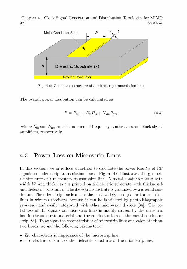
92Chapter 4. Clock Signal Generation and Distribution Topologies for MIMO
Systems
Ground Conductor
Dielectric Substrate ( )b
WMetal Conductor Strip t
Fig. 4.6: Geometric structure of a microstrip transmission line.
The overall power dissipation can be calculated as
P = PLO + NfsPfs + NamPam, (4.3)
where Nfs and Nam are the numbers of frequency synthesizers and clock signalamplifiers, respectively.
4.3 Power Loss on Microstrip Lines
In this section, we introduce a method to calculate the power loss Ptl of RFsignals on microstrip transmission lines. Figure 4.6 illustrates the geomet-ric structure of a microstrip transmission line. A metal conductor strip withwidth W and thickness t is printed on a dielectric substrate with thickness band dielectric constant ε. The dielectric substrate is grounded by a ground con-ductor. The microstrip line is one of the most widely used planar transmissionlines in wireless receivers, because it can be fabricated by photolithographicprocesses and easily integrated with other microwave devices [84]. The to-tal loss of RF signals on microstrip lines is mainly caused by the dielectricloss in the substrate material and the conductor loss on the metal conductorstrip [84]. To analyze the characteristics of microstrip lines and calculate thesetwo losses, we use the following parameters:
• Z0: characteristic impedance of the microstrip line;• ε: dielectric constant of the dielectric substrate of the microstrip line;
4.3 Power Loss on Microstrip Lines 93
• b: thickness of the dielectric substrate;• tan δ: loss tangent of the dielectric material used in the substrate;• t: thickness of the metal conductor strip;• W : width of the metal conductor strip;• ρ: resistivity of the metal conductor strip material;• Rs: surface resistance of the metal conductor strip;• µ0: permeability of vacuum, µ0 = 4π × 10−7H/m;• c: speed of light, c = 3× 10⁸m/s;• fc: carrier frequency of the received signal;• λ: wavelength of the received signal λ = c
fc.
4.3.1 Microstrip Line Analysis Using Quasi-static Method
In the analysis of the characteristics of microstrip lines using a quasi-staticmethod, the propagation mode of electro-magnetic (EM) waves on the mi-crostrip lines is assumed to be purely Transverse Electro Magnetic (TEM) orvery close to TEM (quasi-TEM) [85] [86]. The analysis using this method isfound to be accurate for frequencies below the X-band (8 GHz to 12 GHz). Inthe quasi-static method, both the characteristic impedance and the effectivedielectric constant of microstrip lines are considered invariant to frequency.
We assume a characteristic impedance Z0 of 50 Ω. Given Z0 and dielectricconstant ε, the line width can be found by [84] [86]:
W
b=
8 exp(A)
exp(2A)−2 for Wb < 2,
2π
[B − 1− ln(2B − 1) + ε−1
2ε
ln(B − 1) + 0.39− 0.61
ε
]for W
b > 2.
(4.4)In (4.4),
A , Z0
60
√ε + 1
2+
ε− 1ε + 1
(0.23 +
0.11ε
), and
B , 377π
2Z0√
ε.
Having determined the width W of the microstrip line, the effective dielectric
94Chapter 4. Clock Signal Generation and Distribution Topologies for MIMO
Systems
constant can be approximated by [87]
εe =ε + 1
2+
ε− 12
F (W/b), (4.5)
where
F (W/b) =
1√1+12b/W
+ 0.04(1−W/b)2 for Wb ≤ 1,
1√1+12b/W
for Wb ≥ 1.
Both (4.4) and (4.5) are based on the assumption of infinitely thin metal con-ductor strip thickness, i.e. t ≈ 0. For metal conductor strip with finite thick-ness t, the effective width of the metal conductor strip We can be calculatedas [88]
We =
W + 1.25π t
[1 + ln
(4πW
t
)]for W
b ≤ 1/2π,
W + 1.25π t
[1 + ln
(2bt
)]for W
b ≥ 1/2π.(4.6)
The characteristic impedance can then be obtained as [88]
Z0e =
60√εe
ln(
8bWe
+ We4b
)for W
b ≤ 1,120π√
εe[We/b+1.393+0.667 ln(We/b+1.444)] for Wb ≥ 1,
(4.7)
where εe is the effective dielectric constant given by
εe =ε + 1
2+
ε− 12
F (W/b)− C, (4.8)
withC =
ε + 14.6
t/b√W/b
.
4.3.2 Microstrip Line Analysis using Dispersion Models
The quasi-static method does not consider the non-TEM propagation modeon microstrip lines. The non-TEM propagation mode causes both the effec-tive dielectric constant εe and the characteristic impedance Z0e to become
4.3 Power Loss on Microstrip Lines 95
frequency-dependent. This effect is known as dispersion. The dispersion ef-fect becomes non-negligible for millimeter waves, i.e. for frequencies in theorder of tens of GHz and above. Exact evaluation of the effect of dispersionrequires a full wave analysis of the microstrip configuration which is complexand normally does not lead to any closed-form solutions [86]. To simplifythe analysis, several quasi-empirical models, also known as dispersion mod-els, were developed in the literature to provide closed-form solutions on thefrequency dependency of εe and Z0e .
An accurate dispersion model for the frequency-dependent effective dielectricconstant εe(f) was developed by Kobayashi [89] and can be expressed as:
εe(f) = ε− ε− εe1 + (f/f50)
m , (4.9)
wheref50 =
fk,TM0
0.75 + [0.75− (0.332/ε1.73)]W/b,
fk,TM0 =c tan−1
(ε√
εe−1ε−εe
)
2πb√
ε− εe,
m = m0mc,
m0 = 1 +1
1 +√
W/b+ 0.32
(1
1 +√
W/h
)3
, and
mc =
1 + 1.4
1+W/b
[0.15− 0.235 exp
(−0.45f
f50
)]for W
b ≤ 0.7,
1 for Wb > 0.7.
A dispersion model for the frequency-dependent characteristic impedance Z0e(f)was developed by Hammerstad and Jensen [90] and is given by
Z0e(f) = Z0eεe(f)− 1
εe − 1
√εe
εe(f). (4.10)
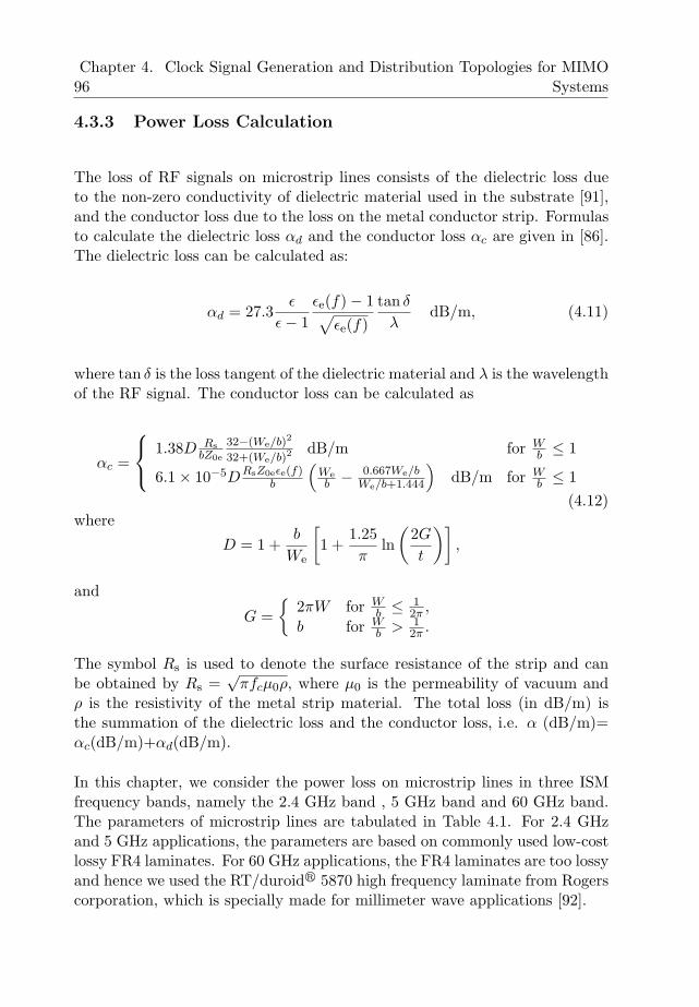
96Chapter 4. Clock Signal Generation and Distribution Topologies for MIMO
Systems
4.3.3 Power Loss Calculation
The loss of RF signals on microstrip lines consists of the dielectric loss dueto the non-zero conductivity of dielectric material used in the substrate [91],and the conductor loss due to the loss on the metal conductor strip. Formulasto calculate the dielectric loss αd and the conductor loss αc are given in [86].The dielectric loss can be calculated as:
αd = 27.3ε
ε− 1εe(f)− 1√
εe(f)tan δ
λdB/m, (4.11)
where tan δ is the loss tangent of the dielectric material and λ is the wavelengthof the RF signal. The conductor loss can be calculated as
αc =
1.38D RsbZ0e
32−(We/b)2
32+(We/b)2dB/m for W
b ≤ 1
6.1× 10⁻⁵DRsZ0eεe(f)b
(Web − 0.667We/b
We/b+1.444
)dB/m for W
b ≤ 1(4.12)
where
D = 1 +b
We
[1 +
1.25π
ln(
2G
t
)],
and
G =
2πW for Wb ≤ 1
2π ,
b for Wb > 1
2π .
The symbol Rs is used to denote the surface resistance of the strip and canbe obtained by Rs =
√πfcµ0ρ, where µ0 is the permeability of vacuum and
ρ is the resistivity of the metal strip material. The total loss (in dB/m) isthe summation of the dielectric loss and the conductor loss, i.e. α (dB/m)=αc(dB/m)+αd(dB/m).
In this chapter, we consider the power loss on microstrip lines in three ISMfrequency bands, namely the 2.4 GHz band , 5 GHz band and 60 GHz band.The parameters of microstrip lines are tabulated in Table 4.1. For 2.4 GHzand 5 GHz applications, the parameters are based on commonly used low-costlossy FR4 laminates. For 60 GHz applications, the FR4 laminates are too lossyand hence we used the RT/duroidr 5870 high frequency laminate from Rogerscorporation, which is specially made for millimeter wave applications [92].
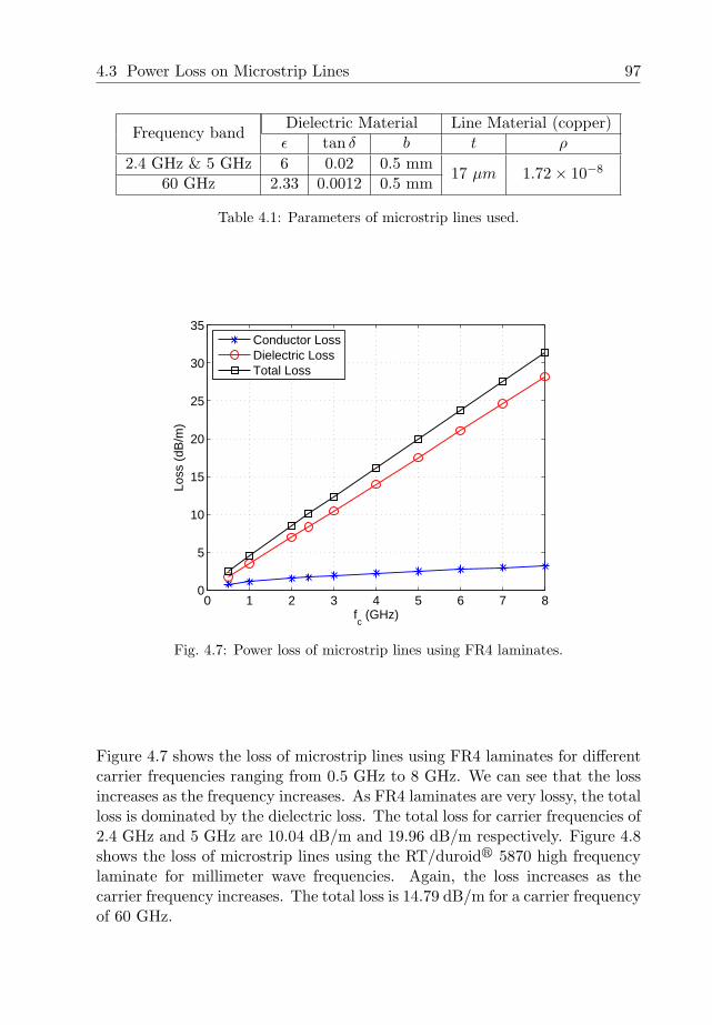
4.3 Power Loss on Microstrip Lines 97
Frequency bandDielectric Material Line Material (copper)ε tan δ b t ρ
2.4 GHz & 5 GHz 6 0.02 0.5 mm17 µm 1.72× 10⁻⁸
60 GHz 2.33 0.0012 0.5 mm
Table 4.1: Parameters of microstrip lines used.
0 1 2 3 4 5 6 7 80
5
10
15
20
25
30
35
fc (GHz)
Loss
(dB
/m)
Conductor LossDielectric LossTotal Loss
Fig. 4.7: Power loss of microstrip lines using FR4 laminates.
Figure 4.7 shows the loss of microstrip lines using FR4 laminates for differentcarrier frequencies ranging from 0.5 GHz to 8 GHz. We can see that the lossincreases as the frequency increases. As FR4 laminates are very lossy, the totalloss is dominated by the dielectric loss. The total loss for carrier frequencies of2.4 GHz and 5 GHz are 10.04 dB/m and 19.96 dB/m respectively. Figure 4.8shows the loss of microstrip lines using the RT/duroidr 5870 high frequencylaminate for millimeter wave frequencies. Again, the loss increases as thecarrier frequency increases. The total loss is 14.79 dB/m for a carrier frequencyof 60 GHz.
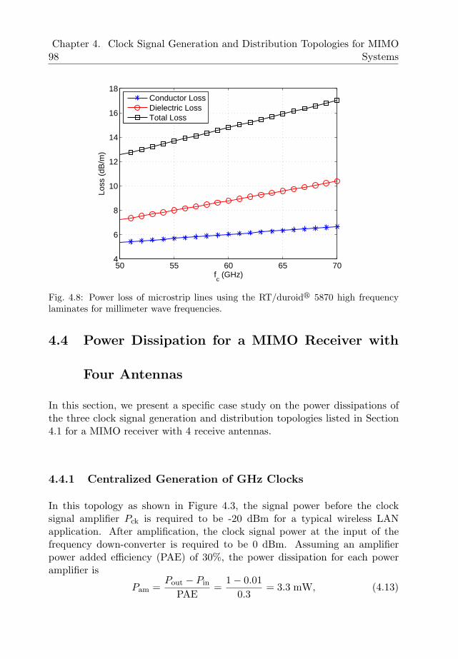
98Chapter 4. Clock Signal Generation and Distribution Topologies for MIMO
Systems
50 55 60 65 704
6
8
10
12
14
16
18
fc (GHz)
Loss
(dB
/m)
Conductor LossDielectric LossTotal Loss
Fig. 4.8: Power loss of microstrip lines using the RT/duroidr 5870 high frequencylaminates for millimeter wave frequencies.
4.4 Power Dissipation for a MIMO Receiver with
Four Antennas
In this section, we present a specific case study on the power dissipations ofthe three clock signal generation and distribution topologies listed in Section4.1 for a MIMO receiver with 4 receive antennas.
4.4.1 Centralized Generation of GHz Clocks
In this topology as shown in Figure 4.3, the signal power before the clocksignal amplifier Pck is required to be -20 dBm for a typical wireless LANapplication. After amplification, the clock signal power at the input of thefrequency down-converter is required to be 0 dBm. Assuming an amplifierpower added efficiency (PAE) of 30%, the power dissipation for each poweramplifier is
Pam =Pout − Pin
PAE=
1− 0.010.3
= 3.3 mW, (4.13)
4.4 Power Dissipation for a MIMO Receiver with Four Antennas 99
and the number of amplifiers needed Nam = 4.
Assuming the distance between the centralized clock and the clock signalamplifier at the antenna is d meters, the loss on the transmission line isPtl = [α(fc)× d] dB. As the RF splitter needs to split one common clocksignal to 4 branches, the total splitter loss is Psp = 1.5 + 10 log10 4 = 7.5dB. Therefore, the clock signal power required at the output of the frequencysynthesizer is
PLO = Pck + Ptl + Psp = −20 + α(fc)× d + 7.5= [−12.5 + α(fc)× d] dBm. (4.14)
For centralized clock-signal generation, only one frequency synthesizer is re-quired, i.e. Nfs = 1. In this chapter, we assume that the power dissipation ofthe frequency synthesizer Pfs = 17 mW, which is typical for a wireless LANreceiver. Therefore, the total power dissipation for this topology is given by
P = PLO + NfsPfs + NamPam
= 0.056× 10α(fc)d/10 + 1× 17 + 4× 3.3=
[0.056× 10α(fc)d/10 + 30.2
]mW. (4.15)
4.4.2 Distributed Generation of GHz Clocks
In this topology as shown in Figure 4.4, only a MHz reference clock signalis generated centrally and distributed to different receive antennas. Due tothe low frequency of the reference clock signal, the loss on microstrip linesis negligible. The splitter loss is 7.5 dB and is the same as for topology A.Therefore, the LO output signal power is
PLO = Pck + Ptl + Psp = −20 + 0 + 7.5= −12.5 dBm = 0.056 mW. (4.16)
Similar to topology A, an amplifier is required to amplify the clock signal tothe desired 0 dBm power level. The power dissipation of the amplifier is the
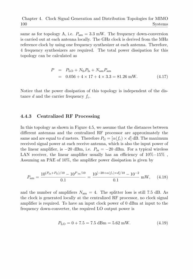
100Chapter 4. Clock Signal Generation and Distribution Topologies for MIMO
Systems
same as for topology A, i.e. Pam = 3.3 mW. The frequency down-conversionis carried out at each antenna locally. The GHz clock is derived from the MHzreference clock by using one frequency synthesizer at each antenna. Therefore,4 frequency synthesizers are required. The total power dissipation for thistopology can be calculated as
P = PLO + NfsPfs + NamPam
= 0.056 + 4× 17 + 4× 3.3 = 81.26 mW. (4.17)
Notice that the power dissipation of this topology is independent of the dis-tance d and the carrier frequency fc.
4.4.3 Centralized RF Processing
In this topology as shown in Figure 4.5, we assume that the distances betweendifferent antennas and the centralized RF processor are approximately thesame and are equal to d meters. Therefore Ptl = [α(fc)× d] dB. The maximumreceived signal power at each receive antenna, which is also the input power ofthe linear amplifier, is −20 dBm, i.e. Pin = −20 dBm. For a typical wirelessLAN receiver, the linear amplifier usually has an efficiency of 10%−15% ,Assuming an PAE of 10%, the amplifier power dissipation is given by
Pam =10(Pin+Ptl)/10 − 10P in/10
0.1=
10[−20+α(fc)×d]/10 − 10−2
0.1mW, (4.18)
and the number of amplifiers Nam = 4. The splitter loss is still 7.5 dB. Asthe clock is generated locally at the centralized RF processor, no clock signalamplifier is required. To have an input clock power of 0 dBm at input to thefrequency down-converter, the required LO output power is
PLO = 0 + 7.5 = 7.5 dBm = 5.62 mW. (4.19)
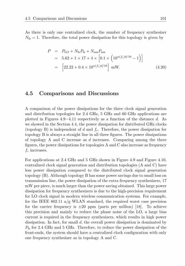
4.5 Comparisons and Discussions 101
As there is only one centralized clock, the number of frequency synthesizerNfs = 1. Therefore, the total power dissipation for this topology is given by
P = PLO + NfsPfs + NamPam
= 5.62 + 1× 17 + 4×[0.1×
(10α(fc)d/10 − 1
)]
=[22.22 + 0.4× 10α(fc)d/10
]mW. (4.20)
4.5 Comparisons and Discussions
A comparison of the power dissipations for the three clock signal generationand distribution topologies for 2.4 GHz, 5 GHz and 60 GHz applications areplotted in Figures 4.9−4.11 respectively as a function of the distance d. Aswe showed in the Section 4.4, the power dissipation for distributed GHz clocks(topology B) is independent of d and fc. Therefore, the power dissipation fortopology B is always a straight line in all three figures. The power dissipationsof topology A and C increase as d increases. Comparing among the threefigures, the power dissipations for topologies A and C also increase as frequencyfc increases.
For applications at 2.4 GHz and 5 GHz shown in Figure 4.9 and Figure 4.10,centralized clock signal generation and distribution topologies (A and C) haveless power dissipation compared to the distributed clock signal generationtopology (B). Although topology B has some power savings due to small loss ontransmission line, the power dissipation of the extra frequency synthesizers, 17mW per piece, is much larger than the power saving obtained. This large powerdissipation for frequency synthesizers is due to the high-precision requirementfor LO clock signal in modern wireless communication systems. For example,for the IEEE 802.11 a/g WLAN standard, the required worst case precisionfor the carrier frequency is ±20 ppm (parts per million) [18]. To achievethis precision and mainly to reduce the phase noise of the LO, a large biascurrent is required in the frequency synthesizers, which results in high powerdissipation. In fact, for small d, the overall power dissipation is dominated byPfs for 2.4 GHz and 5 GHz. Therefore, to reduce the power dissipation of thefront-ends, the system should have a centralized clock configuration with onlyone frequency synthesizer as in topology A and C.
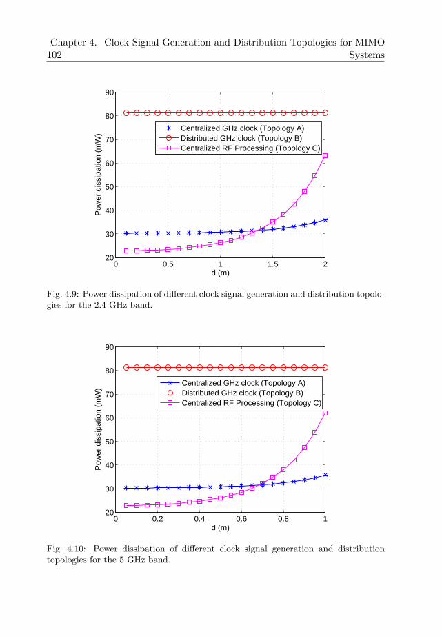
102Chapter 4. Clock Signal Generation and Distribution Topologies for MIMO
Systems
0 0.5 1 1.5 220
30
40
50
60
70
80
90
d (m)
Pow
er d
issi
patio
n (m
W)
Centralized GHz clock (Topology A)Distributed GHz clock (Topology B)Centralized RF Processing (Topology C)
Fig. 4.9: Power dissipation of different clock signal generation and distribution topolo-gies for the 2.4 GHz band.
0 0.2 0.4 0.6 0.8 120
30
40
50
60
70
80
90
d (m)
Pow
er d
issi
patio
n (m
W)
Centralized GHz clock (Topology A)Distributed GHz clock (Topology B)Centralized RF Processing (Topology C)
Fig. 4.10: Power dissipation of different clock signal generation and distributiontopologies for the 5 GHz band.
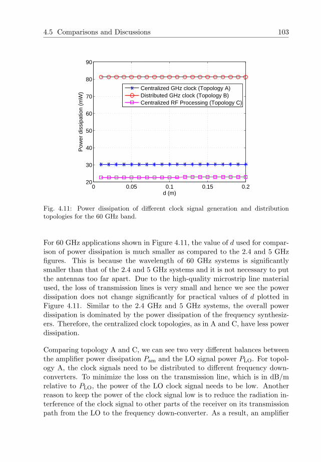
4.5 Comparisons and Discussions 103
0 0.05 0.1 0.15 0.220
30
40
50
60
70
80
90
d (m)
Pow
er d
issi
patio
n (m
W)
Centralized GHz clock (Topology A)Distributed GHz clock (Topology B)Centralized RF Processing (Topology C)
Fig. 4.11: Power dissipation of different clock signal generation and distributiontopologies for the 60 GHz band.
For 60 GHz applications shown in Figure 4.11, the value of d used for compar-ison of power dissipation is much smaller as compared to the 2.4 and 5 GHzfigures. This is because the wavelength of 60 GHz systems is significantlysmaller than that of the 2.4 and 5 GHz systems and it is not necessary to putthe antennas too far apart. Due to the high-quality microstrip line materialused, the loss of transmission lines is very small and hence we see the powerdissipation does not change significantly for practical values of d plotted inFigure 4.11. Similar to the 2.4 GHz and 5 GHz systems, the overall powerdissipation is dominated by the power dissipation of the frequency synthesiz-ers. Therefore, the centralized clock topologies, as in A and C, have less powerdissipation.
Comparing topology A and C, we can see two very different balances betweenthe amplifier power dissipation Pam and the LO signal power PLO. For topol-ogy A, the clock signals need to be distributed to different frequency down-converters. To minimize the loss on the transmission line, which is in dB/mrelative to PLO, the power of the LO clock signal needs to be low. Anotherreason to keep the power of the clock signal low is to reduce the radiation in-terference of the clock signal to other parts of the receiver on its transmissionpath from the LO to the frequency down-converter. As a result, an amplifier
104Chapter 4. Clock Signal Generation and Distribution Topologies for MIMO
Systems
with large gain, hence large power dissipation, is needed at each frequencydown-converter to amplify the clock signal to the desired power level. Here,the power dissipation of the amplifier Pam is fixed while the power of the LOsignals PLO is dependent on d and fc. For topology C, the frequency down-conversion is carried out locally at the centralized RF processor. Therefore,the LO clock signal can be generated directly to meet the power requirementof the frequency down-converter. The LO signal power PLO is thus fixed. Thelinear amplifiers in topology C need to compensate the loss on the transmis-sion line, hence, Pam is dependent on d and fc. Comparing (4.15) and (4.20),we can see that for small d, the overall power dissipation is dominated by thed-independent power and topology C consumes less power. As d increases,the loss on the transmission line increases. For topology C, this loss is com-pensated using a linear amplifier. As the efficiency of this linear amplifier islower than the clock signal amplifier used in topology A and B, more poweris needed to amplify the signal by the same amount. Therefore, the powerdissipation of topology C increases at a faster rate with respect to d. Hence,for larger d, topology A consumes less power.
In summary, we can see that for the typical system studied, the power dissipa-tion of frequency synthesizers dominates the overall power dissipation in theRF front-end. At a result, for a MIMO receiver, the centralized clock signalgeneration and distribution, which uses only one frequency synthesizer, haslower power dissipation compared to distributed clock signal generation. Inthis chapter, as an example, we only considered a very specific system setupusing microstrip lines with fixed parameters. In practice, the designer shouldrecalculate the power dissipations using the general model in Section 4.2 withsystem specific parameters and determine which topology gives the least powerdissipation.
Besides power dissipation, there are other practical considerations that affectthe choice of clock signal generation and distribution topologies. For example,in a receiver using topology A or C, sophisticated design efforts are needed tohandle the GHz RF signals distributed in the receiver. Special care needs to betaken for shielding these signals to avoid interference to the other parts of thereceiver. Moreover expensive materials are needed to reduce the loss of theseRF signals. In topology B, the RF clock signal generation and frequencydown-conversion are both performed locally at each antenna. As a result,there is no RF signals being transmitted in the system. Hence, requirementson shielding are greatly relaxed and cheaper material can be used. In this case,the distributed clock signal generation has the potential to greatly reduce thedesign complexity and the receiver cost.
4.6 Conclusions 105
4.6 Conclusions
In this chapter, we studied the pros and cons of different clock signal generationand distribution topologies in a MIMO receiver. We proposed a general systemmodel to calculate the power dissipation of a MIMO RF front-end using thesetopologies. We compared the power dissipations for three commonly usedclock signal generation and distribution topologies for a MIMO receiver with4 antennas for different carrier frequencies. The results showed that for thetypical system setup studied, the frequency synthesizer dominates the overallpower dissipation of the front-end. As a result, centralized clock generationand distribution topologies, where only one frequency synthesizer is used, haveless power dissipation compared to distributed clock generation topologies,where multiple frequency synthesizers are needed. However, the distributedclock generation topologies have the potential to reduce the complexity andcost of the receiver front-end because the frequency down-conversion is doneat the antennas and there are no GHz RF signals distributed in the system.

106Chapter 4. Clock Signal Generation and Distribution Topologies for MIMO
Systems
Chapter 5CFO Estimation for MIMO-OFDM
Systems
5.1 Introduction
Multiple-input multiple-output systems increase the capacity of rich scatter-ing wireless fading channels enormously by using multiple antennas at boththe transmitter and the receiver [24] [25] [81]. Most of the early studies on thecapacity of MIMO systems were based on the assumption of flat-fading chan-nels. For frequency-selective fading channels, combining MIMO with OFDMprovides an effective solution. MIMO-OFDM transforms a frequency selec-tive MIMO system to a number of flat fading MIMO systems on differentsubcarriers. Therefore, MIMO-OFDM has been adopted in various industrialstandards for wireless communications, such as IEEE 802.11n high-throughputwireless LAN [5], IEEE 802.16 WiMAX [19] and 3GPP long term evolution(3GPP-LTE) [26].
Similar to single-input single-output (SISO) OFDM systems, carrier frequencyoffset (CFO) is still a major impairment for MIMO-OFDM systems. It de-
108 Chapter 5. CFO Estimation for MIMO-OFDM Systems
stroys the orthogonality between different subcarriers and causes inter-carrierinterference (ICI). ICI can cause severe degradation to the system performanceif not properly compensated. Therefore, accurate estimation and compen-sation of CFO is essential for both SISO and MIMO OFDM systems. Forsingle-user MIMO-OFDM systems, as we have shown in Chapter 4, a central-ized clock generation topology requires lower power dissipation compared toa distributed clock generation topology. In the centralized clock generationtopology, all the transmit antennas are driven by a centralized local oscilla-tor (LO) and so are all the receive antennas. As a result, the CFO betweenthe transmitter LO and the receiver LO is a single scalar parameter. Hence,the CFO estimation in this system is very similar to SISO-OFDM systems.Some CFO estimation algorithms for MIMO-OFDM systems are proposedin [34] [49] [50] [93].
Channel estimation for MIMO-OFDM systems is more complicated than forSISO-OFDM systems. For a MIMO-OFDM system with nt transmit and nr
receive antennas, nr×nt channel responses must be estimated per subcarrier.To estimate the channel responses between a certain receive antenna and dif-ferent transmit antennas using training sequences, the receiver must be able todistinguish between the training sequences from different transmit antennas.Therefore, for training-based channel estimation, some orthogonality amongtraining sequences from different transmit antennas is required. In [52], afrequency-domain orthogonal training sequence design is proposed. The train-ing sequences from different transmit antennas occupy different subcarriers.The length of the training sequence must be at least nt OFDM symbols to getthe channel estimate on all the subcarriers. Another approach uses orthogonalWalsh-Hadamard spreading codes to spread one training sequence to differ-ent OFDM symbols such that the training sequences from different transmitantennas are orthogonal in the code domain [5] [94]. This approach againrequires a training sequence of at least nt OFDM symbols. Both approachesrequire significantly larger overhead for channel estimation compared to SISO-OFDM systems. In [93], a time domain training sequence design is proposedfor MIMO-OFDM systems. This time domain approach requires only train-ing sequences of length nt × L, where L is the length of the channel impulseresponse and is much smaller than the OFDM symbol length. However, theproposed training sequences are impulses in time and hence have very highpeak to average power ratio (PAPR).
In this chapter, we propose to use constant amplitude zero autocorrelation(CAZAC) sequences, which have constant amplitude elements and zero auto-correlation for any nonzero circular shifts, for joint CFO and channel estima-
5.1 Introduction 109
tion for MIMO-OFDM systems. We first formulate the Maximum-Likelihood(ML) CFO and channel estimator. Similar to [49] [50], we show that MLCFO estimate can be obtained with low computational complexity by trans-mitting two periods of the same training sequence. After compensating theestimated CFO, the channel estimation can be performed in the time domain.The advantages of the proposed training sequences are:
• One training sequence for both CFO and channel estimation.• No calculation of matrix inversion is required to obtain channel estimates.• Significantly reduced training overhead. The minimum length required for
channel estimation is only nt × L.• The PAPR of the training sequence in time domain is 1.
The residual CFO after CFO compensation degrades the performance of thechannel estimation. In this chapter, we also derive an approximation on themean square error (MSE) of channel estimation in the presence of the residualCFO. We show from computer simulations that this approximation is accu-rate. From the approximation, we can see that the degradation caused by theresidual CFO in the channel estimation is negligible.
In the study of MIMO and MIMO-OFDM systems, a common assumptionused in the literature is that the channel responses between different trans-mit and receive antennas are statistically independent. In practice, due tothe close proximity among the antennas, the channel responses are spatiallycorrelated [53] [55] [95]. The spatial correlation is related to the propagationenvironment. It is a function of the distributions of angle of arrival (AOA)at the receive antennas and the angle of departure (AOD) at the transmitantennas. Besides this spatial correlation, the electromagnetic (EM) fields atclosely-placed antennas also interact with each other and cause mutual cou-pling among the antennas [56] [57]. This coupling changes the spatial corre-lation and also the power of the transmitted/received signals at the antennas.In this chapter, we present a study on the effects of spatial correlation and mu-tual coupling and in particular, their impacts on the performance of the CFOestimation. The simulation results show that spatial correlation degrades theperformance of the CFO estimation. Mutual coupling has two effects. Firstlyit reduces the spatial correlation, which is beneficial. On the other hand, italso reduces the power of the desired signal, which is detrimental. Simula-tions results show that the combined effects of mutual coupling introducesadditional degradation on CFO estimation.
The rest of this chapter is organized as follows. In Section 5.2, we developthe system model for the MIMO-OFDM system and derive the ML CFO
110 Chapter 5. CFO Estimation for MIMO-OFDM Systems
and channel estimators. We then propose the CAZAC training sequence andderive the simplified ML CFO and channel estimators in Section 5.3. We alsoshow that using the proposed training sequence, the training overhead canbe significantly reduced compared to conventional frequency-domain training.In Section 5.4 we analyze the MSE of the channel estimation in the presenceof the residual CFO. An accurate closed-form approximation on the MSE isderived. Simulation results on the performance of the joint CFO and channelestimator are presented in Section 5.5. In Section 5.6, we study the effect ofspatial correlations and its impact on the performance of CFO estimation. Theeffect of mutual coupling is studied in Section 5.7. The concluding remarksare given in Section 5.8.
5.2 System Model
In this chapter, we study a single-user MIMO-OFDM system with a centralizedclock at both the transmitter and the receiver. In this case, the CFO can bequantified by a single parameter φ. We assume perfect timing synchronizationhas been achieved. In this case, the received signal at the ith receive antennacan be written as
ri(k) = ejφk 1√nt
nt∑
m=1
L−1∑
d=0
hi,m(d)sm(k − d) + ni(k), (5.1)
where k is the time index, nt is the number of transmit antennas, L is thelength of the impulse response of the multi-path channel, hi,m(d) is the dthtap of the channel impulse response between the ith receive antenna and themth transmit antenna, sm is the transmitted signal from the mth transmitantenna and ni(k) is the AWGN noise. Here we assume that the power of sm
for all m is 1, and 1/√
nt is used to normalize the total transmission powerfrom all antennas to 1. We consider a training sequence of length N and cyclicprefix (CP) of length L. After removing the cyclic prefix, we can write thereceived signal at the ith receive antenna in an equivalent matrix form as
ri =1√nt
nt∑
m=1
E(φ)Smhi,m + ni (5.2)
5.2 System Model 111
where E(φ) is the CFO matrix, which is a diagonal matrix with diagonalelements equal to [1, exp(jφ), · · · , exp(j(N − 1)φ)]. We use Sm to denote thetransmitted signal matrix from the mth transmit antenna. This is a circulantmatrix with the first column defined by [sm(0), sm(1), · · · , sm(N−1)]T , wherewe use superscript T to denote vector/matrix transpose. Here we assumeN > L, so the channel vector between the mth transmit antenna and theith receive antenna hi,m is a N × 1 vector obtained by appending the L × 1channel impulse response [hi,m(0), · · · , hi,m(L− 1)]T vector with N −L zeros,i.e. hi,m = [hi,m(0), · · · , hi,m(L − 1), 0, · · · , 0]T . The AWGN noise at the ithreceive antenna is denoted as ni.
Gathering the received signal from all the receive antennas, we get
R = E(φ)SH + N , (5.3)
whereR = [r1 · · · , rnr ]N×nr ,
S =1√nt
[S1, · · · ,Snt ]N×(N×nt)
H =
H1...
Hnt
(N×nt)×nr
,
with Hi = [h1,i, · · · ,hnr,i]N×nr. For ease of understanding, we use a sub-script inside curved brackets to denote dimensions of matrices. The noisematrix is given by N = [n1, · · · ,nnr ].
Because the noise is Gaussian and uncorrelated, the likelihood function for theCFO φ and the channel matrix H can be written as
Λ(φ, H) =1
(πσ2n)N×nr
exp− 1
σ2n
∥∥∥R−E(φ)SH∥∥∥
2
, (5.4)
where φ and H are trial values for φ and H and σ2n is the variance of the re-
ceiver AWGN noise. The maximum-likelihood estimates for CFO and channelcan be obtained by finding the φ and H that maximize (5.4).
112 Chapter 5. CFO Estimation for MIMO-OFDM Systems
5.3 CAZAC Sequences for Joint CFO and Channel
Estimation
We propose to use constant amplitude zero autocorrelation (CAZAC) se-quences for joint CFO and channel estimation in MIMO-OFDM systems. Eachelement of a CAZAC sequence has a amplitude equal to one, i.e. constant am-plitude. The autocorrelation of a length-N CAZAC sequence s1 satisfies
R(k) =N−1∑
n=0
s1(n)s∗1(nª k) =
N k = 0;0 k 6= 0.
(5.5)
where ª denotes circular subtraction and superscript ∗ denotes complex con-jugation. This means that the CAZAC sequence is orthogonal to all non-zerocircular shifts. Let S1 be a circulant matrix with the first column equal to[s1(0), s1(1), · · · , s1(N − 1)]T . The autocorrelation property of the CAZACsequence can be written in an equivalent matrix form as
SH1 S1 = NI, (5.6)
where superscript H denotes conjugate transpose. This means that S1 is botha unitary (subject to a normalization constant N) and a circulant matrix.Commonly used CAZAC sequences include the Frank-Zadoff sequences [96],the Chu sequences [97] and the S&H sequences [98].
We use s1 as the training sequence from the first transmit antenna. Thetraining sequence from the mth transmit antenna is a circularly shifted versionof s1, i.e. sm(n) = [s1(n ª τm)]T , where τm is the shift value. It is straight-forward to show that the cross-correlation between the training sequences fromdifferent transmit antennas satisfies
SHi Sj = Iτj−τi (5.7)
where Iτj−τi denotes a matrix resulting from circularly shifting the one ele-ments of the identify matrix to the right by τj − τi. Note that the matrixSm can be obtained by circularly shifting the rows of S1 τm rows downwards.
5.3 CAZAC Sequences for Joint CFO and Channel Estimation 113
Hence, we haveSmhi,m = S1hτm
i,m, (5.8)
where hτmi,m = [hi,m(N − τm), · · · , hi,m(0), · · ·hi,m(N − τm−1)]T is obtained by
circularly shifting hi,m τm rows downwards. Making use of this property, wecan rewrite the received signal at receive antenna i as
ri =1√nt
E(φ)nt∑
m=1
Smhi,m =1√nt
E(φ)S1
nt∑
m=1
hτmi,m. (5.9)
Collecting the received signals from all receive antennas, we get
R =1√nt
E(φ)S1H+ N , (5.10)
where
H =
[nt∑
m=1
hτm1,m,
nt∑
m=1
hτm2,m, · · · ,
nt∑
m=1
hτmnr,m
]
N×nr.
From (5.10), we can see that by using CAZAC training sequence, the channelimpulse responses are contained in a smaller matrix H of size N × nr ascompare to the (N × nt)× nr channel matrix H in the more general receivedsignal model in (5.3).
Without loss of generality, let us examine the first column of the H matrix,∑ntm=1 hτm
1,m. We know that only the first L elements in the N × 1 vectorh1,m are nonzero. We choose the length of the CAZAC sequence N such thatN ≥ nt × L and we can make τm − τm−1 ≥ L for m = 2, · · · , nt. In thiscase, there will be no overlap between the non-zero channel impulse responsesfrom different transmit antennas. As a result, after obtaining the estimateof the first column of H, i.e.
∑ntm=1 hτm
1,m, we can obtain the channel impulseresponses from different transmit antennas by taking appropriate elements ofthe column. The same principle applies to the other columns of H. In thiscase, the estimation of the channel impulse responses between all the transmitand receive antenna pairs is converted equivalently to the estimation of matrixH.
In [38] and [39], CFO estimation methods using periodic training sequences
114 Chapter 5. CFO Estimation for MIMO-OFDM Systems
were proposed. Here, we adopt a similar approach. We successively transmittwo periods of training sequences in time, i.e. the training sequence from theith transmit antenna, xi = [sT
i , sTi ]T , is of length 2N . Assuming the channel
does not change within the duration of 2N , the received signal can be writtenas:
R2N×nr = E(φ)2N×2NX2N×NHN×nr + N 2N×nr, (5.11)
where
X =1√nt
[S1
S1
].
Using the received signal model given in (5.11), the likelihood function of theCFO φ and the channel response H can be written as
Λ(φ, H) =1
(πσ2n)2N×nr
exp− 1
σ2n
tr
[R−E(φ)XH]H
[R−E(φ)XH]
(5.12)
where tr denotes the trace of a matrix.
Following a similar approach as in [45], we find that by keeping φ fixed, theML estimate of the channel H is given by
H(φ) =(XHX
)−1XHEH(φ)R. (5.13)
Substituting (5.13) into (5.12), and after some algebraic manipulations we getthe ML estimator of the CFO φ is given by
φ = arg maxφ
tr
RHE(φ)BEH(φ)R
, (5.14)
5.3 CAZAC Sequences for Joint CFO and Channel Estimation 115
where
B = X(XHX
)−1XH =
12N
[S1
S1
]IN×N
[SH
1 ,SH1
]
=12
[IN×N IN×NIN×N IN×N
]. (5.15)
We can also rewrite E(φ) and R in the following form
E(φ) =[
E1(φ) 00 ejNφE1(φ)
],
where E1(φ) = diag[1, ejφ, · · · , ej(N−1)φ] and
R =[ R1
R2
],
where R1 denotes the first N rows of R and R2 denotes rows N + 1 to 2Nof R. Substituting these new expressions into (5.14), we can further simplifythe cost function for CFO estimation to
J (φ) = <
ejNφtr(RH2 R1)
, (5.16)
where <(•) denotes the real part of a complex number. Correspondingly, theML estimate of φ is given by
φ = arg maxφ<
ejNφtr(RH
2 R1)
. (5.17)
Using scalar notations, the ML CFO estimator in (5.17) can be written equiv-alently as
φ =1N
∠
N∑
k=1
nr∑
m=1
r∗m(k)rm(k + N)
, (5.18)
116 Chapter 5. CFO Estimation for MIMO-OFDM Systems
where ∠(•) denotes the angle of a complex number and rm(k) denotes thereceived signal from the mth receive antenna at time k. This ML estimate isvery similar in form to its SISO counterpart as shown in [39] [45] and it canbe easily obtained using low-complexity correlation operations.
The performance of the ML CFO estimator for SISO-OFDM systems hasbeen extensively studied in the literature [38], [39], [45]. Following a similarapproach as in SISO-OFDM systems, we can show that the Cramer-Rao Bound(CRB) of the CFO estimation is given by [50]
E[(φ− φ)2] ≥ CRB =1
nrN3γ, (5.19)
where γ is the SNR per receive antenna. Notice that the CRB decays withN3 and hence in practice, only small values of N are needed.
Having obtained the CFO estimate φ, we can simply plug it into (5.13) to getthe channel estimate as follows
H =(XHX
)−1XHEH(φ)R =
nt
2NXHEH(φ)R
=√
nt
2N
[SH
1 ,SH1
][
EH1 (φ) 00 e−jNφEH
1 (φ)
][ R1
R2
]
=√
nt
2N
(SH
1 EH1 (φ)R1 + e−jNφSH
1 EH1 (φ)R2
). (5.20)
From (5.20), we can see that the channel estimate can be obtained using sim-ple matrix multiplications. Due to the orthogonal property of the S1 matrix,a complicated matrix inversion can be avoided. This provides a large savingin the computational complexity of channel estimation. Another advantageof this training sequence is the low overhead. For channel estimation alone,we only need training sequences of length N where N ≥ nt × L. By compar-ison, the conventional frequency-domain channel estimation requires trainingsequence of length at least nt × M , where M is the length of the OFDMsymbol. In a practical OFDM system, the length L of the channel impulseresponse is similar to the length of the cyclic prefix, which is much smallerthan the length of the OFDM symbol M . Therefore, by using the proposedtraining sequence for channel estimation, we can reduce the training overheadby a factor of (M/L− 1). Moreover, the training signal is constant-amplitude
5.4 MSE Analysis of Channel Estimation with Residual CFO 117
in time and therefore has peak to average power ratio equal to 1.
5.4 MSE Analysis of Channel Estimation with Resid-
ual CFO
In practical systems, there exists some residual CFO after CFO compensationdue to the inaccuracy of the CFO estimation. In this section, we examine howthe residual CFO affects the performance of the channel estimation.
Substituting the expression for R1 and R2 into (5.20) and denoting the resid-ual CFO (φ− φ) by φd, we get
H =1
2N
(SH
1 E1(φd)S1H+√
ntSH1 EH
1 (φ)N 1
+ ejNφdSH1 E1(φd)S1H+ e−jNφ√ntSH
1 EH1 (φ)N 2
),
(5.21)
where N 1 contains the first N rows of N in (5.11) and N 2 contains rows N +1to 2N of N . As EH
1 (φ) is a unitary matrix, EH1 (φ)N 1 is statistically the same
as N 1. Similarly e−jNφEH1 (φ)N 2 is statistically the same as N 2. Therefore,
for ease of notation, we still use N 1 and N 2 to denote the new noise. Withthis simplification of notation, the channel estimate can be rewritten as
H =1
2N
(1 + ejNφd
)SH
1 E1(φd)S1H+√
nt
2N(SH
1 N 1 + SH1 N 2). (5.22)
The MSE of the channel estimation is given by
MSE =1
Nnrtr
E
[(H− H)H(H− H)
], (5.23)
where E[•] denotes statistical expectation over the AWGN noise.
118 Chapter 5. CFO Estimation for MIMO-OFDM Systems
When the CFO estimation is perfect, i.e. φd = 0, it can be easily shown that
MSE =nt
4N2
1Nnr
trE
[N H1 S1SH
1 N 1
]+ E
[N H2 S1SH
1 N 2
]
=ntσ
2n
2N. (5.24)
Making use of the Taylor’s series expansion, we can write the exponentialfunction as eφ = 1 +
∑∞k=1
φk
k! . Substituting this into (5.22), we get
H =1 + δ
NSH
1 (I + ∆(φd))S1H+N ′
N, (5.25)
where δ = 1/2∑∞
k=1(jNφd)k
k! and ∆(φd) is a diagonal matrix with the nth
element equal to∑∞
k=1(j(n−1)φd)k
k! . Here we use one AWGN noise matrix N ′
to denote√
nt
2 (SH1 N 1 +SH
1 N 2). Note that the variance of each element of N ′
is Nnt2 σ2
n. Using this new expression, we can write the difference between thechannel estimate and the actual channel as
H − H =N ′
N+Hδ +
1 + δ
NSH
1 ∆(φd)S1H. (5.26)
Here the first term N ′N is the estimation error caused by the AWGN noise
while the last two terms in the summation describe the extra estimation errorcaused by the residual CFO error φd.
Using (5.26), we can show that the MSE of the channel estimation is given by
MSE =1
N3nr
N2|δ|2tr ΨH+ 2N< [
(δ∗ + |δ|2)tr [∆(φd)S1ΨHSH
1
]]
+ |1 + δ|2tr [∆(φd)H∆(φd)S1ΨHSH
1
]+
ntσ2n
2N.
(5.27)
where ΨH = E(HHH). The details of the derivation is given in the ap-
5.4 MSE Analysis of Channel Estimation with Residual CFO 119
pendix of this chapter. Now let us assume that the channels between differ-ent transmit and receive antennas are uncorrelated in space and the differentpaths in the multi-path channel are also uncorrelated. We define pi,m =[pi,m(1), · · · , pi,m(N)]T as the power delay profile of the channel between themth transmit antenna and the ith receive antenna. Since the length of thechannel impulse response is L, pi,m(N) = 0 for N > L− 1. Using this, we canwrite
ΨH = E(HHH) = diag
[nt∑
i=1
(nr∑
k=1
pk,i(nª τi)
)], (5.28)
where pk,i(nªτi) denotes a vector obtained by circularly shift pk,i τi elementsdownwards. We normalize the channel such that the total transmit signalpower equals the receive signal power per receive antenna. As a result, thepower of the channel taps between all the transmit and receive antenna pairsadds up to nt × nr. Therefore, we have
tr[ΨH] = ntnr.
We further define F = S1ΨHSH1 . It can be shown that the ith diagonal
element of F, F (i, i) is given by
F (i, i) =N∑
m=1
Ψ(j, j) = tr[ΨH] = ntnr. (5.29)
As ∆(φd) is a diagonal matrix, we have
tr[∆(φd)S1ΨHSH
1
]= ntnrtr [∆(φd)] ,
and similarly
tr[∆(φd)H∆(φd)S1ΨHSH
1
]= ntnrtr
[∆(φd)H∆(φd)
].
As we are going to show later from the simulations, the performance of CFOestimation reaches the CRB at SNRs of practical interest. Therefore, the
120 Chapter 5. CFO Estimation for MIMO-OFDM Systems
residual CFO value φd is usually very small. We can use a first-order Taylorseries expansion to get a good approximation of the exponential function, i.e.δ = 1/2
∑∞k=1
(jNφd)k
k! ≈ jNφd/2 and ∆(φd) ≈ diag[0, jφd, j2φd, · · · , j(N −1)φd]. Substituting these into (5.27), we get
MSE =ntσ
2n
2N+ 2<
(N − 1)φ2
dnt
4+
jN(N − 1)φ3dnt
8
+(
1 +N2φ2
d
4
)nt(N − 1)(2N − 1)φ2
d
6N2+
ntNφ2d
4
=ntσ
2n
2N+
nt
(9N3 − 2N2 − 6N + 2
)
12N2φ2
d +nt(N − 1)(2N − 1)
24φ4
d
≈ ntσ2n
2N+
nt
(9N3 − 2N2 − 6N + 2
)
12N2φ2
d. (5.30)
Here we drop the φ4d term in the MSE expression because the estimation error
φd is very small in practical SNR regions and higher-order terms have onlynegligible contribution to the overall MSE. As we are going to show laterusing simulations, the variance of φd touches the CRB at moderate to highSNR regions. Therefore, we can approximate φ2
d in (5.30) with the CRBexpression, i.e.
φ2d ≈
1nrN3γ
.
Substituting this into (5.30), we get the MSE of channel estimation in thepresence of residual CFO φd given by
MSE ≈ ntσ2n
2N+
nt
(9N3 − 2N2 − 6N + 2
)
12N5γnr
= σ2n
(nt
2N+
nt
(9N3 − 2N2 − 6N + 2
)
12N5nr
). (5.31)
The first term in (5.31) is the MSE due to the AWGN noise while the secondterm is the extra MSE caused by the residual CFO φd. The ratio between
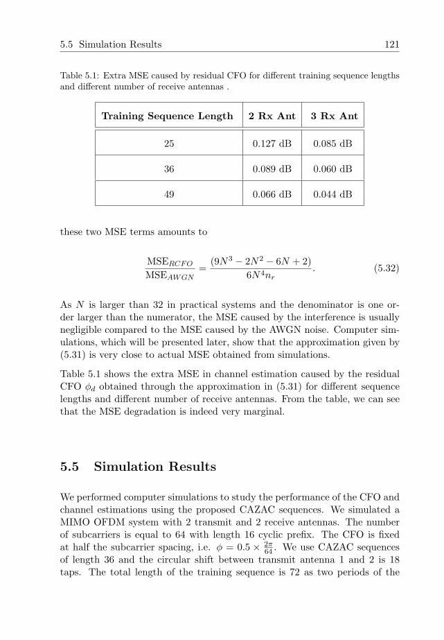
5.5 Simulation Results 121
Table 5.1: Extra MSE caused by residual CFO for different training sequence lengthsand different number of receive antennas .
Training Sequence Length 2 Rx Ant 3 Rx Ant
25 0.127 dB 0.085 dB
36 0.089 dB 0.060 dB
49 0.066 dB 0.044 dB
these two MSE terms amounts to
MSERCFO
MSEAWGN=
(9N3 − 2N2 − 6N + 2)6N4nr
. (5.32)
As N is larger than 32 in practical systems and the denominator is one or-der larger than the numerator, the MSE caused by the interference is usuallynegligible compared to the MSE caused by the AWGN noise. Computer sim-ulations, which will be presented later, show that the approximation given by(5.31) is very close to actual MSE obtained from simulations.
Table 5.1 shows the extra MSE in channel estimation caused by the residualCFO φd obtained through the approximation in (5.31) for different sequencelengths and different number of receive antennas. From the table, we can seethat the MSE degradation is indeed very marginal.
5.5 Simulation Results
We performed computer simulations to study the performance of the CFO andchannel estimations using the proposed CAZAC sequences. We simulated aMIMO OFDM system with 2 transmit and 2 receive antennas. The numberof subcarriers is equal to 64 with length 16 cyclic prefix. The CFO is fixedat half the subcarrier spacing, i.e. φ = 0.5 × 2π
64 . We use CAZAC sequencesof length 36 and the circular shift between transmit antenna 1 and 2 is 18taps. The total length of the training sequence is 72 as two periods of the
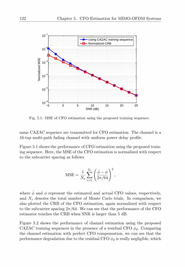
122 Chapter 5. CFO Estimation for MIMO-OFDM Systems
−5 0 5 10 15 20 2510
−6
10−5
10−4
10−3
10−2
10−1
SNR (dB)
Nor
mal
ized
MS
E
Using CAZAC training sequenceNormalized CRB
Fig. 5.1: MSE of CFO estimation using the proposed training sequence.
same CAZAC sequence are transmitted for CFO estimation. The channel is a16-tap multi-path fading channel with uniform power delay profile.
Figure 5.1 shows the performance of CFO estimation using the proposed train-ing sequence. Here, the MSE of the CFO estimation is normalized with respectto the subcarrier spacing as follows
MSE =1
Ns
Ns∑
i=1
(φ− φ
2π/64
)2
,
where φ and φ represent the estimated and actual CFO values, respectively,and Ns denotes the total number of Monte Carlo trials. In comparison, wealso plotted the CRB of the CFO estimation, again normalized with respectto the subcarrier spacing 2π/64. We can see that the performance of the CFOestimator touches the CRB when SNR is larger than 5 dB.
Figure 5.2 shows the performance of channel estimation using the proposedCAZAC training sequences in the presence of a residual CFO φd. Comparingthe channel estimation with perfect CFO compensation, we can see that theperformance degradation due to the residual CFO φd is really negligible, which
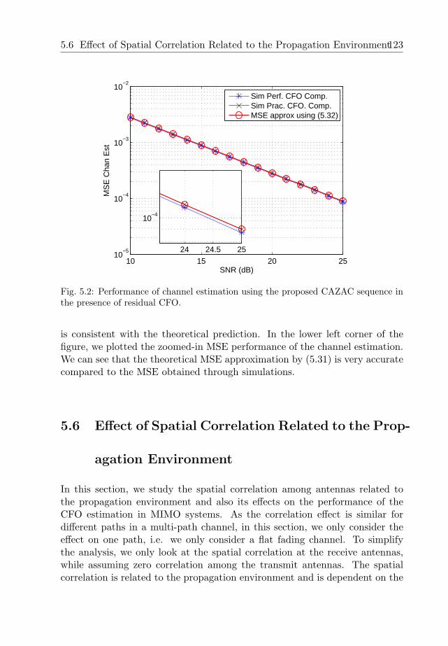
5.6 Effect of Spatial Correlation Related to the Propagation Environment123
10 15 20 2510
−5
10−4
10−3
10−2
SNR (dB)
MS
E C
han
Est
Sim Perf. CFO Comp.Sim Prac. CFO. Comp.MSE approx using (5.32)
24 24.5 25
10−4
Fig. 5.2: Performance of channel estimation using the proposed CAZAC sequence inthe presence of residual CFO.
is consistent with the theoretical prediction. In the lower left corner of thefigure, we plotted the zoomed-in MSE performance of the channel estimation.We can see that the theoretical MSE approximation by (5.31) is very accuratecompared to the MSE obtained through simulations.
5.6 Effect of Spatial Correlation Related to the Prop-
agation Environment
In this section, we study the spatial correlation among antennas related tothe propagation environment and also its effects on the performance of theCFO estimation in MIMO systems. As the correlation effect is similar fordifferent paths in a multi-path channel, in this section, we only consider theeffect on one path, i.e. we only consider a flat fading channel. To simplifythe analysis, we only look at the spatial correlation at the receive antennas,while assuming zero correlation among the transmit antennas. The spatialcorrelation is related to the propagation environment and is dependent on the
124 Chapter 5. CFO Estimation for MIMO-OFDM Systems
distributions of angle of arrival (AOA) and angle of departure (AOD), whichare specified by the power angular spectrum (PAS). We study how PAS affectsthe performance of CFO estimation. For a Laplacian PAS, which is a goodmodel for the indoor propagation environment [99] [100], we also study howthe performance of CFO estimation is affected by the mean AOA values.
We consider a MIMO system with Nt transmit and Nr receive antennas in flatfading channels. The received signal on nr receive antennas can be written as
r = Hs + n (5.33)
where s is the transmitted signal from nt transmit antennas, H is the nr × nt
channel matrix with the i, jth element Hi,j as the channel response betweenthe jth transmit antenna and the ith receive antenna and n is the AWGNnoise. In practice, MIMO channels are correlated in the spatial domain. Suchcorrelation can be modeled as [101]
H = [Rrx]1/2 Hiid
([Rtx]
1/2)T
, (5.34)
where Hiid is the channel matrix generated using independent, identically, dis-tributed (i.i.d.) zero-mean complex Gaussian random variables. The transmitand receive correlation matrices are denoted as Rtx and Rrx respectively. Fora 3× 3 channel, the two matrices take on the following form [101]
Rtx =
1 ρtx,1,2 ρtx,1,3
ρtx,2,1 1 ρtx,2,3
ρtx,3,1 ρtx,3,2 1
,
Rrx =
1 ρrx,1,2 ρrx,1,3
ρrx,2,1 1 ρrx,2,3
ρrx,3,1 ρrx,3,2 1
, (5.35)
where ρtx,i,j is the correlation coefficient between the ith and jth transmitantennas and ρrx,i,j is the correlation coefficient between the ith and jth receiveantennas. The spatial correlation is determined by the PAS of AOA at thereceiver and the PAS of the AOD at the transmitter.
In the derivation of the spatial correlation, we consider a two-antenna receiver
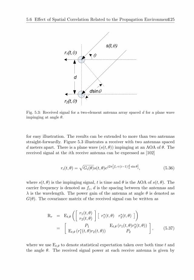
5.6 Effect of Spatial Correlation Related to the Propagation Environment125
s(t,
d
dsin
r1(t,
r2(t,
Fig. 5.3: Received signal for a two-element antenna array spaced d for a plane waveimpinging at angle θ.
for easy illustration. The results can be extended to more than two antennasstraight-forwardly. Figure 5.3 illustrates a receiver with two antennas spacedd meters apart. There is a plane wave (s(t, θ)) impinging at an AOA of θ. Thereceived signal at the ith receive antenna can be expressed as [102]
ri(t, θ) =√
Gi(θ)s(t, θ)ej2π[fc+(i−1) dλ
sin θ], (5.36)
where s(t, θ) is the impinging signal, t is time and θ is the AOA of s(t, θ). Thecarrier frequency is denoted as fc, d is the spacing between the antennas andλ is the wavelength. The power gain of the antenna at angle θ is denoted asG(θ). The covariance matrix of the received signal can be written as
Rr = Et,θ
([r1(t, θ)r2(t, θ)
] [r∗1(t, θ) r∗2(t, θ)
])
=[
P1 Et,θ (r1(t, θ)r∗2(t, θ))Et,θ (r∗1(t, θ)r2(t, θ)) P2
], (5.37)
where we use Et,θ to denote statistical expectation taken over both time t andthe angle θ. The received signal power at each receive antenna is given by
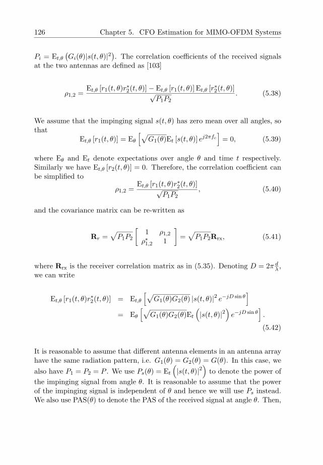
126 Chapter 5. CFO Estimation for MIMO-OFDM Systems
Pi = Et,θ
(Gi(θ)|s(t, θ)|2
). The correlation coefficients of the received signals
at the two antennas are defined as [103]
ρ1,2 =Et,θ [r1(t, θ)r∗2(t, θ)]− Et,θ [r1(t, θ)] Et,θ [r∗2(t, θ)]√
P1P2. (5.38)
We assume that the impinging signal s(t, θ) has zero mean over all angles, sothat
Et,θ [r1(t, θ)] = Eθ
[√G1(θ)Et [s(t, θ)] ej2πfc
]= 0, (5.39)
where Eθ and Et denote expectations over angle θ and time t respectively.Similarly we have Et,θ [r2(t, θ)] = 0. Therefore, the correlation coefficient canbe simplified to
ρ1,2 =Et,θ [r1(t, θ)r∗2(t, θ)]√
P1P2, (5.40)
and the covariance matrix can be re-written as
Rr =√
P1P2
[1 ρ1,2
ρ∗1,2 1
]=
√P1P2Rrx, (5.41)
where Rrx is the receiver correlation matrix as in (5.35). Denoting D = 2π dλ ,
we can write
Et,θ [r1(t, θ)r∗2(t, θ)] = Et,θ
[√G1(θ)G2(θ) |s(t, θ)|2 e−jD sin θ
]
= Eθ
[√G1(θ)G2(θ)Et
(|s(t, θ)|2
)e−jD sin θ
].
(5.42)
It is reasonable to assume that different antenna elements in an antenna arrayhave the same radiation pattern, i.e. G1(θ) = G2(θ) = G(θ). In this case, wealso have P1 = P2 = P . We use Ps(θ) = Et
(|s(t, θ)|2
)to denote the power of
the impinging signal from angle θ. It is reasonable to assume that the powerof the impinging signal is independent of θ and hence we will use Ps instead.We also use PAS(θ) to denote the PAS of the received signal at angle θ. Then,
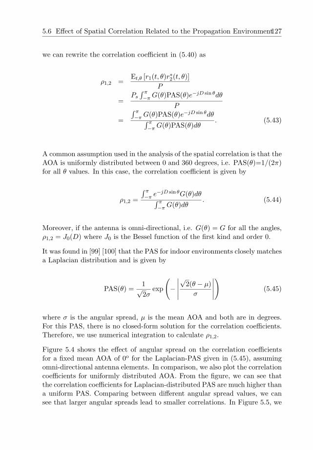
5.6 Effect of Spatial Correlation Related to the Propagation Environment127
we can rewrite the correlation coefficient in (5.40) as
ρ1,2 =Et,θ [r1(t, θ)r∗2(t, θ)]
P
=Ps
∫ π−π G(θ)PAS(θ)e−jD sin θdθ
P
=
∫ π−π G(θ)PAS(θ)e−jD sin θdθ∫ π
−π G(θ)PAS(θ)dθ. (5.43)
A common assumption used in the analysis of the spatial correlation is that theAOA is uniformly distributed between 0 and 360 degrees, i.e. PAS(θ)=1/(2π)for all θ values. In this case, the correlation coefficient is given by
ρ1,2 =
∫ π−π e−jD sin θG(θ)dθ∫ π
−π G(θ)dθ. (5.44)
Moreover, if the antenna is omni-directional, i.e. G(θ) = G for all the angles,ρ1,2 = J0(D) where J0 is the Bessel function of the first kind and order 0.
It was found in [99] [100] that the PAS for indoor environments closely matchesa Laplacian distribution and is given by
PAS(θ) =1√2σ
exp
(−
∣∣∣∣∣
√2(θ − µ)
σ
∣∣∣∣∣
)(5.45)
where σ is the angular spread, µ is the mean AOA and both are in degrees.For this PAS, there is no closed-form solution for the correlation coefficients.Therefore, we use numerical integration to calculate ρ1,2.
Figure 5.4 shows the effect of angular spread on the correlation coefficientsfor a fixed mean AOA of 0o for the Laplacian-PAS given in (5.45), assumingomni-directional antenna elements. In comparison, we also plot the correlationcoefficients for uniformly distributed AOA. From the figure, we can see thatthe correlation coefficients for Laplacian-distributed PAS are much higher thana uniform PAS. Comparing between different angular spread values, we cansee that larger angular spreads lead to smaller correlations. In Figure 5.5, we
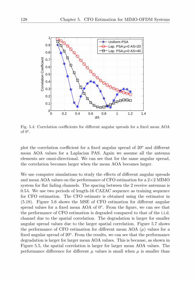
128 Chapter 5. CFO Estimation for MIMO-OFDM Systems
0 0.2 0.4 0.6 0.8 1 1.2 1.40
0.1
0.2
0.3
0.4
0.5
0.6
0.7
0.8
0.9
1
d/λ
Cor
rela
tion
Coe
ffici
ent
Uniform PSALap. PSA µ=0 AS=20Lap. PSA µ=0 AS=40
Fig. 5.4: Correlation coefficients for different angular spreads for a fixed mean AOAof 0o.
plot the correlation coefficient for a fixed angular spread of 20o and differentmean AOA values for a Laplacian PAS. Again we assume all the antennaelements are omni-directional. We can see that for the same angular spread,the correlation becomes larger when the mean AOA becomes larger.
We use computer simulations to study the effects of different angular spreadsand mean AOA values on the performance of CFO estimation for a 2×2 MIMOsystem for flat fading channels. The spacing between the 2 receive antennas is0.5λ. We use two periods of length-16 CAZAC sequence as training sequencefor CFO estimation. The CFO estimate is obtained using the estimator in(5.18). Figure 5.6 shows the MSE of CFO estimation for different angularspread values for a fixed mean AOA of 0o. From the figure, we can see thatthe performance of CFO estimation is degraded compared to that of the i.i.d.channel due to the spatial correlation. The degradation is larger for smallerangular spread values due to the larger spatial correlation. Figure 5.7 showsthe performance of CFO estimation for different mean AOA (µ) values for afixed angular spread of 20o. From the results, we can see that the performancedegradation is larger for larger mean AOA values. This is because, as shown inFigure 5.5, the spatial correlation is larger for larger mean AOA values. Theperformance difference for different µ values is small when µ is smaller than
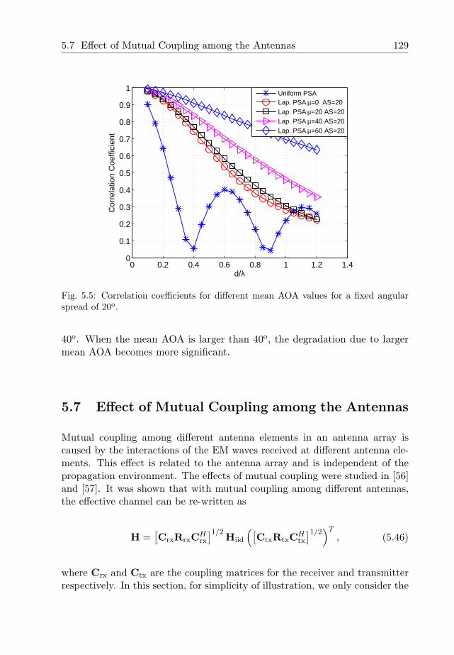
5.7 Effect of Mutual Coupling among the Antennas 129
0 0.2 0.4 0.6 0.8 1 1.2 1.40
0.1
0.2
0.3
0.4
0.5
0.6
0.7
0.8
0.9
1
d/λ
Cor
rela
tion
Coe
ffici
ent
Uniform PSALap. PSA µ=0 AS=20Lap. PSA µ=20 AS=20Lap. PSA µ=40 AS=20Lap. PSA µ=60 AS=20
Fig. 5.5: Correlation coefficients for different mean AOA values for a fixed angularspread of 20o.
40o. When the mean AOA is larger than 40o, the degradation due to largermean AOA becomes more significant.
5.7 Effect of Mutual Coupling among the Antennas
Mutual coupling among different antenna elements in an antenna array iscaused by the interactions of the EM waves received at different antenna ele-ments. This effect is related to the antenna array and is independent of thepropagation environment. The effects of mutual coupling were studied in [56]and [57]. It was shown that with mutual coupling among different antennas,the effective channel can be re-written as
H =[CrxRrxCH
rx
]1/2Hiid
([CtxRtxCH
tx
]1/2)T
, (5.46)
where Crx and Ctx are the coupling matrices for the receiver and transmitterrespectively. In this section, for simplicity of illustration, we only consider the
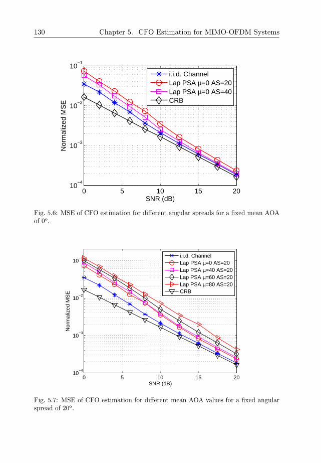
130 Chapter 5. CFO Estimation for MIMO-OFDM Systems
0 5 10 15 2010
−4
10−3
10−2
10−1
SNR (dB)
Nor
mal
ized
MS
E
i.i.d. ChannelLap PSA µ=0 AS=20Lap PSA µ=0 AS=40CRB
Fig. 5.6: MSE of CFO estimation for different angular spreads for a fixed mean AOAof 0o.
0 5 10 15 2010
−4
10−3
10−2
10−1
SNR (dB)
Nor
mal
ized
MS
E
i.i.d. ChannelLap PSA µ=0 AS=20Lap PSA µ=40 AS=20Lap PSA µ=60 AS=20Lap PSA µ=80 AS=20CRB
Fig. 5.7: MSE of CFO estimation for different mean AOA values for a fixed angularspread of 20o.
5.7 Effect of Mutual Coupling among the Antennas 131
effects of propagation environments and mutual coupling at the receiver. Inthis case, the effective channel can be simplified to
H =[CRCH
]1/2Hiid. (5.47)
Here we dropped the subscript of rx for simplicity of illustration. In [58] [59][104], it was shown that mutual coupling reduces the spatial correlation be-tween the antennas. On the other hand, mutual coupling also results in powerloss on the desired signal when the two antennas are placed too close [105].Next, we look at the overall effects of mutual coupling on the performance ofCFO estimation in MIMO systems.
In this study, we consider a receiver with two dipole antennas with the follow-ing parameters:
• l: length of the dipole antenna;• D: D = 2π d
λ where d is the spacing between the two antennas and λ is thewavelength;
• Zs = Rs + jXs: self impedance of the antenna;• Zm = Rm + jXm: mutual impedance between the antennas due to mutual
coupling;• Zload = Rload + jXload: loading impedance of the antennas.
From [56], the coupling matrix in (5.47) is given by
C = (Zload + Zs)[
Zload + Zs Zm
Zm Zload + Zs
]−1
. (5.48)
In this study, we assume that the loading impedance is matched to the selfimpedance of the antenna, i.e. Zload = Z∗s . The mutual impedance Zm is afunction of the dipole length l, the antenna spacing D and the antenna place-ment configuration. The mutual impedance can be calculated numericallyusing the induced Electromagnetic Fields (EMF) method [106]. Combiningthe effect of coupling with the spatial correlation related to the propagation
132 Chapter 5. CFO Estimation for MIMO-OFDM Systems
environment, we have
CRCH =[
C1,1 C1,2
C2,1 C2,2
] [1 ρ1,2
ρ2,1 1
] [C∗
1,1 C∗2,1
C∗1,2 C∗
2,2
]
= P
[1 ρ1,2
ρ2,1 1
]. (5.49)
From (5.49), we can see that there are two effects from mutual coupling.Firstly, the mutual coupling changes the spatial correlation. Secondly, thereceived signal power is scaled by P .
The effective correlation (|ρ1,2|) as a function of the antenna spacing for a2-antenna receiver is depicted in Figure 5.8. Here, we assume two dipoleantennas with length l = 0.5λ placed side by side. For such antennas, the self-impedance is Zs = (73 + j42)Ω [106]. We also assume that the AOA has auniform distribution from 0 to 360o. We can see that with the effect of mutualcoupling, the spatial correlation between the antennas is reduced. The powerP as a function of the antenna spacing is shown in Figure 5.9. The plot showsthat the system suffers significant power loss if the two antennas are spacedtoo closely. The power loss becomes insignificant when the antenna spacingis about 1λ. In summary, the effect of mutual coupling is two-fold. Firstlyit reduces the spatial correlation between the antennas, which is a desirableeffect. On the other hand, it introduces extra power loss, which is undesirable.
We used computer simulations to investigate the combined effect of mutualcoupling on the performance of the CFO estimation. We simulated a 2 × 2MIMO system for flat fading channels. We assume the transmit antennasare independent and only consider the effect of coupling at the receiver. Thespacing between two receive antenna is 0.5λ. We also assume an uniformlydistributed AOA at the receiver. The performance of CFO estimation with andwithout considering the effect of coupling is compared in Figure 5.10. We cansee that the spatial correlation introduced by the propagation environmentdegrades the MSE performance as compared to the i.i.d. channel. Mutualcoupling adds additional degradation to the performance. This means thatthe detrimental effect due to the power loss (as shown in Figure 5.9) is largerthan the beneficial effect due to reduced spatial correlation (as shown in Figure5.8).
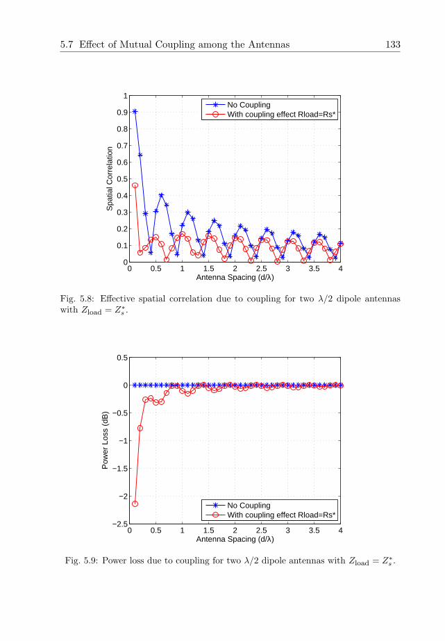
5.7 Effect of Mutual Coupling among the Antennas 133
0 0.5 1 1.5 2 2.5 3 3.5 40
0.1
0.2
0.3
0.4
0.5
0.6
0.7
0.8
0.9
1
Antenna Spacing (d/λ)
Spa
tial C
orre
latio
n
No CouplingWith coupling effect Rload=Rs*
Fig. 5.8: Effective spatial correlation due to coupling for two λ/2 dipole antennaswith Zload = Z∗s .
0 0.5 1 1.5 2 2.5 3 3.5 4−2.5
−2
−1.5
−1
−0.5
0
0.5
Antenna Spacing (d/λ)
Pow
er L
oss
(dB
)
No CouplingWith coupling effect Rload=Rs*
Fig. 5.9: Power loss due to coupling for two λ/2 dipole antennas with Zload = Z∗s .
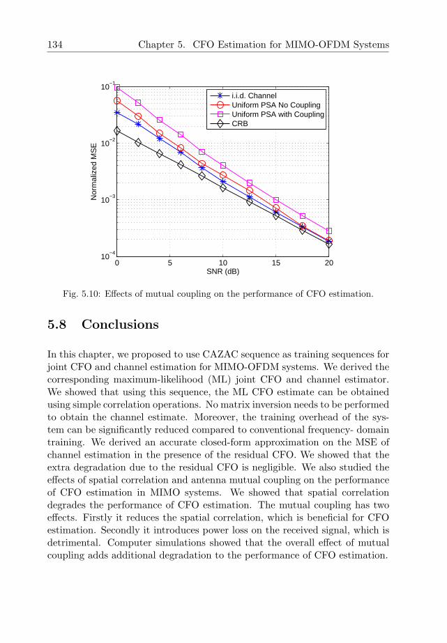
134 Chapter 5. CFO Estimation for MIMO-OFDM Systems
0 5 10 15 2010
−4
10−3
10−2
10−1
SNR (dB)
Nor
mal
ized
MS
E
i.i.d. ChannelUniform PSA No CouplingUniform PSA with CouplingCRB
Fig. 5.10: Effects of mutual coupling on the performance of CFO estimation.
5.8 Conclusions
In this chapter, we proposed to use CAZAC sequence as training sequences forjoint CFO and channel estimation for MIMO-OFDM systems. We derived thecorresponding maximum-likelihood (ML) joint CFO and channel estimator.We showed that using this sequence, the ML CFO estimate can be obtainedusing simple correlation operations. No matrix inversion needs to be performedto obtain the channel estimate. Moreover, the training overhead of the sys-tem can be significantly reduced compared to conventional frequency- domaintraining. We derived an accurate closed-form approximation on the MSE ofchannel estimation in the presence of the residual CFO. We showed that theextra degradation due to the residual CFO is negligible. We also studied theeffects of spatial correlation and antenna mutual coupling on the performanceof CFO estimation in MIMO systems. We showed that spatial correlationdegrades the performance of CFO estimation. The mutual coupling has twoeffects. Firstly it reduces the spatial correlation, which is beneficial for CFOestimation. Secondly it introduces power loss on the received signal, which isdetrimental. Computer simulations showed that the overall effect of mutualcoupling adds additional degradation to the performance of CFO estimation.
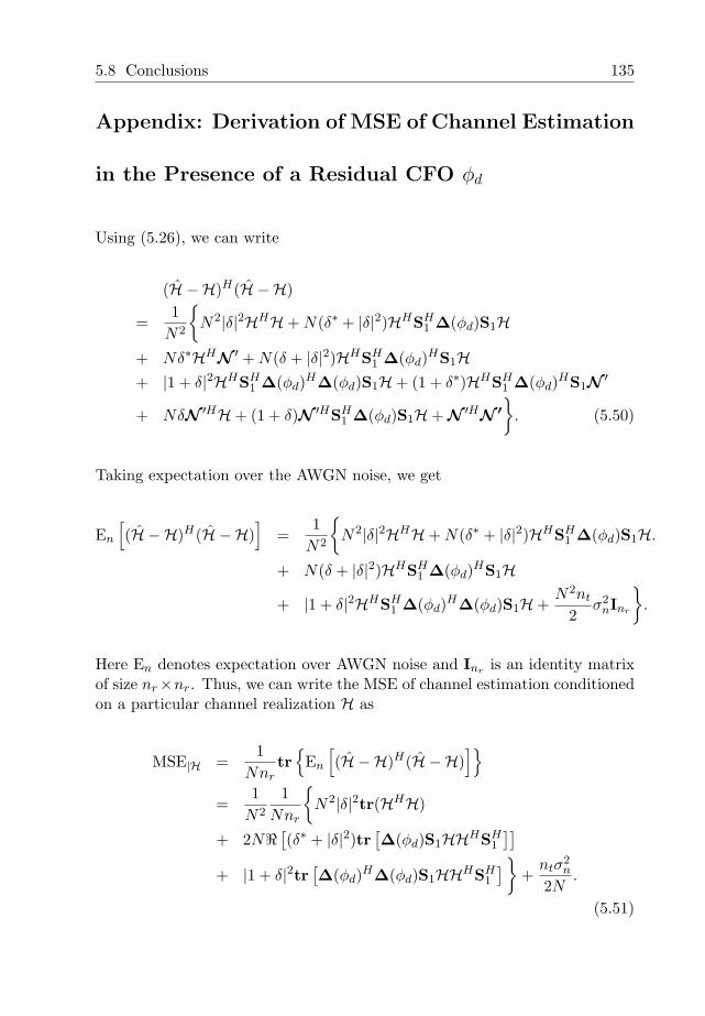
5.8 Conclusions 135
Appendix: Derivation of MSE of Channel Estimation
in the Presence of a Residual CFO φd
Using (5.26), we can write
(H − H)H(H − H)
=1
N2
N2|δ|2HHH+ N(δ∗ + |δ|2)HHSH
1 ∆(φd)S1H
+ Nδ∗HHN ′ + N(δ + |δ|2)HHSH1 ∆(φd)HS1H
+ |1 + δ|2HHSH1 ∆(φd)H∆(φd)S1H+ (1 + δ∗)HHSH
1 ∆(φd)HS1N ′
+ NδN ′HH+ (1 + δ)N ′HSH1 ∆(φd)S1H+ N ′HN ′
. (5.50)
Taking expectation over the AWGN noise, we get
En
[(H − H)H(H − H)
]=
1N2
N2|δ|2HHH+ N(δ∗ + |δ|2)HHSH
1 ∆(φd)S1H.
+ N(δ + |δ|2)HHSH1 ∆(φd)HS1H
+ |1 + δ|2HHSH1 ∆(φd)H∆(φd)S1H+
N2nt
2σ2
nInr
.
Here En denotes expectation over AWGN noise and Inr is an identity matrixof size nr×nr. Thus, we can write the MSE of channel estimation conditionedon a particular channel realization H as
MSE|H =1
Nnrtr
En
[(H − H)H(H − H)
]
=1
N2
1Nnr
N2|δ|2tr(HHH)
+ 2N< [(δ∗ + |δ|2)tr [
∆(φd)S1HHHSH1
]]
+ |1 + δ|2tr [∆(φd)H∆(φd)S1HHHSH
1
]+
ntσ2n
2N.
(5.51)
136 Chapter 5. CFO Estimation for MIMO-OFDM Systems
Now averaging the MSE of the channel estimation over all the channel real-izations, we get
MSE = EHMSE|H
=1
N3nr
N2|δ|2tr ΨH+ 2N< [
(δ∗ + |δ|2)tr [∆(φd)S1ΨHSH
1
]]
+ |1 + δ|2tr [∆(φd)H∆(φd)S1ΨHSH
1
]+
ntσ2n
2N,
(5.52)
where ΨH = E(HHH).
Chapter 6CFO Estimation for Multi-user
MIMO-OFDM Uplink Using
CAZAC Sequences
6.1 Introduction
The multi-user MIMO-OFDM system can be considered as an extension of theMIMO-OFDM system to the multi-user context. In the multi-user MIMO-OFDM system shown in Figure 6.1, multiple users, each with one or multipleantennas, transmit simultaneously using OFDM in the same frequency band.For clearness of illustration, in Figure 6.1, we only illustrate the case whereeach user has one transmit antenna. The receiver is a base station equippedwith multiple antennas. It uses spatial processing techniques to separate thesignals of different users. If we view the signals from different users as signalsfrom different transmit antennas of a virtual transmitter, then the whole sys-
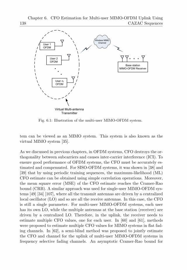
138Chapter 6. CFO Estimation for Multi-user MIMO-OFDM Uplink Using
CAZAC Sequences
User nt
OFDM
User 2
OFDM
User 1
OFDM
Base station
MIMO-OFDM Receiver
Virtual Multi-antenna
Transmitter
Wireless MIMO
Channel
Fig. 6.1: Illustration of the multi-user MIMO-OFDM system.
tem can be viewed as an MIMO system. This system is also known as thevirtual MIMO system [35].
As we discussed in previous chapters, in OFDM systems, CFO destroys the or-thogonality between subcarriers and causes inter-carrier interference (ICI). Toensure good performance of OFDM systems, the CFO must be accurately es-timated and compensated. For SISO-OFDM systems, it was shown in [38] and[39] that by using periodic training sequences, the maximum-likelihood (ML)CFO estimate can be obtained using simple correlation operations. Moreover,the mean square error (MSE) of the CFO estimate reaches the Cramer-Raobound (CRB). A similar approach was used for single-user MIMO-OFDM sys-tems [49] [34] [107], where all the transmit antennas are driven by a centralizedlocal oscillator (LO) and so are all the receive antennas. In this case, the CFOis still a single parameter. For multi-user MIMO-OFDM systems, each userhas its own LO, while the multiple antennas at the base station (receiver) aredriven by a centralized LO. Therefore, in the uplink, the receiver needs toestimate multiple CFO values, one for each user. In [60] and [61], methodswere proposed to estimate multiple CFO values for MIMO systems in flat fad-ing channels. In [62], a semi-blind method was proposed to jointly estimatethe CFO and channel for the uplink of multi-user MIMO-OFDM systems infrequency selective fading channels. An asymptotic Cramer-Rao bound for
6.1 Introduction 139
joint CFO and channel estimation in the uplink of MIMO-Orthogonal Fre-quency Division Multiple Access (OFDMA) system was derived in [108] andtraining strategies that minimize the asymptotic CRB were studied. In [109], areduced-complexity CFO and channel estimator was proposed for the uplink ofMIMO-OFDMA systems using an approximation of the ML cost function anda Newton search algorithm. It was also shown that the reduced-complexitymethod is asymptotically efficient. The joint CFO and channel estimationfor multi-user MIMO-OFDM systems was studied in [63]. Training sequencesthat minimize the asymptotic CRB were also designed in [63].
It is known in the literature that the computational complexity for obtain-ing the ML CFO estimates in the uplink of multi-user MIMO-OFDM systemgrows exponentially with the number of users [63] [109]. A low-complexityalgorithm was proposed in [63] for CFO estimation in the uplink of multi-userMIMO OFDM systems based on importance sampling. However, the complex-ity required to generate sufficient samples for importance sampling may stillbe high for practical implementations. In this chapter, we study algorithmsthat can further reduce the computational complexity of the CFO estimation.In particular, we propose a low-complexity CFO estimation algorithm usingconstant amplitude zero autocorrelation (CAZAC) training sequences. Fol-lowing a similar approach as in [45], we first derive the ML estimator for themultiple CFO values in frequency selective-fading channels. Obtaining theML estimates requires a search over all possible CFO values and the computa-tional complexity is prohibitive for practical implementations. To reduce thecomputational complexity, we propose a sub-optimal algorithm using CAZACtraining sequences. Using the proposed algorithm, the CFO estimates for dif-ferent users can be obtained using simple correlation operations similar tosingle-user MIMO-OFDM systems. Moreover, the computational complexityof the algorithm grows only linearly with the number of users. However, weshow that multiple CFO values in the uplink introduce multiple access interfer-ence (MAI) in the CFO estimation using the proposed algorithm. This causesan irreducible error floor in the MSE performance. We derive an expressionfor the signal to multiple access interference ratio (SIR) in the presence ofmultiple CFO values. To reduce the MAI, we find the training sequences thatmaximize the SIR. Note that the training sequence optimization problem wetry to solve in this chapter is different from those in [63] and [108], wheretraining sequences are optimized to minimize the CRB. In this chapter, wetry to find the training sequences that maximize the SIR due to multiple CFOvalues specially for the proposed low-complexity CFO estimation algorithmusing CAZAC training sequences. The optimal training sequences turn out tobe dependent on the actual CFO values from different users. This is obviously
140Chapter 6. CFO Estimation for Multi-user MIMO-OFDM Uplink Using
CAZAC Sequences
not practical as it is not possible to know the CFO values and hence selectthe optimal training sequences in advance. To remove this dependency, wepropose a new cost function, which is the Taylor’s series approximation of theoriginal cost function. The new cost function is independent of the actual CFOvalues and is an accurate approximation of the original SIR based cost func-tion for small CFO values. Using the new cost function, we obtain the optimaltraining sequences for the following three classes of CAZAC sequences:
• the Frank & Zadoff sequences [96];• the Chu Sequences [97];• the polyphase sequences by Sueshiro and Hatori (S&H Sequences) [98].
Both the Frank & Zadoff sequences and the S&H sequences exist for sequencelength N = K2, where N is the length of the sequence and K is a positiveinteger larger than 1, while Chu sequences exist for any integer length N > 1.For both the Frank & Zadoff and the Chu sequences, there are a finite num-ber of sequences for each sequence length. Therefore, the optimal sequencescan be obtained using an off-line search among these sequences. However, forS& H sequences, there are infinitely many possible sequences. As the opti-mization problem for the S& H sequences cannot be solved analytically, weresort to a numerical method to obtain a near-optimal solution. To this end,we use the adaptive simulated annealing (ASA) technique [110]. For smallsequence lengths, for example N = 16 and N = 36, we are able to use ex-haustive search to verify that the solution obtained using ASA is globallyoptimal. We use computer simulations to evaluate the performance of theproposed CFO estimation algorithm using CAZAC sequences. We first com-pare the performance using CAZAC sequences with the performance using twoother sequences with good correlation properties, namely, the IEEE 802.11nshort training field (STF) [5] and the m sequences [111]. The results showthat the error floor using CAZAC sequences is more than 10 times smallercompared to the other two sequences. Comparing among the three classesof CAZAC sequences, we find that the performance of the Chu sequences isbetter than the Frank & Zadoff sequences due to the larger degree of freedomin the sequence construction. The S&H sequences have the largest number ofdegree of freedom in the construction of the CAZAC sequences. However, thesimulation results show that they have only very marginal performance gaincompared to the Chu sequences. This makes Chu sequences a good choicefor practical implementation due to its simple construction and flexibility insequence lengths. By using the identified optimal sequences, the error floorin the CFO estimation is significantly lower compared to using a randomlyselected CAZAC sequence.
6.2 System Model 141
The rest of this chapter is organized as follows. In Section 6.2, we present thesystem model and derive the ML estimator for the multiple CFO values. Thesub-optimal CFO estimation algorithm using CAZAC sequences is proposedin Section 6.3. The training sequence optimization problem is formulated inSection 6.4 and methods are given to obtain the optimal training sequence.In Section 6.5, we present the computer simulation results and Section 6.6concludes the chapter.
6.2 System Model
In this chapter, we study a multi-user MIMO-OFDM system with nt users. Forsimplicity of illustration and analysis, we assume that each user has a singletransmit antenna. The base station has nr receive antennas, where nr ≥ nt.The received signal at the ith receive antenna can be written as
ri(k) =nt∑
m=1
(ejφmk
L−1∑
d=0
hi,m(d)sm(k − d)
)+ ni(k), (6.1)
where φm is the CFO of the mth user, k is the time index, and L is the lengthof the channel impulse response. The d-th tap of the channel impulse responsebetween the mth user and the ith receive antenna is denoted as hi,m(d), sm
denotes the transmitted signal from the mth user and ni is the additive whiteGaussian noise (AWGN) at the ith receive antenna. Here we assume theinitial phase for each user is absorbed in the channel impulse response. From(6.1), we can see that we have nt different CFO values (φm’s) to estimate. Weconsider a training sequence of length N and cyclic prefix (CP) of length L.The received signal after removal of CP can be written in an equivalent matrixform
ri =nt∑
m=1
E(φm)Smhi,m + ni (6.2)
where ri = [ri(0), · · · , ri(N −1)]T and superscript T denotes vector transpose.The CFO matrix of user m is denoted E(φm) and is a diagonal matrix with di-agonal elements equal to [1, exp(jφm), · · · , exp(j(N−1)φm)]. We use Sm to de-note the transmitted signal matrix for the mth user. This is an N×N circulantmatrix with the first column defined by [sm(0), sm(1), sm(2), · · · , sm(N−1)]T .
142Chapter 6. CFO Estimation for Multi-user MIMO-OFDM Uplink Using
CAZAC Sequences
Here we assume N > L so the channel vector between the mth user and theith receive antenna hi,m is a N × 1 vector by appending the L × 1 channelimpulse response [hi,m(0), · · · , hi,m(L− 1)]T vector with N − L zeros.
Using this system model, the received signals from all nr receive antennas canbe written as
R = A(φ)H + N , (6.3)
whereR = [r1 · · · , rnr ]N×nr ,
A(φ) = [E(φ1)S1, · · · ,E(φnt)Snt ]N×(N×nt) .
For clearness of presentation, we use subscripts inside curved brackets to de-note the sizes of corresponding matrices. The vector φ = [φ1, · · · , φnt ] is theCFO vector containing the CFO values from all users, and the channels of allusers are stacked into the channel matrix H given as
H =
H1...
Hnt
(N×nt)×nr
,
with Hi = [h1,i, · · · ,hnr,i]N×nr being the channel matrix for the ith user.The AWGN noise matrix is given by N = [n1, · · · ,nnr ].
Because the noise is Gaussian and uncorrelated, the likelihood function for thechannel H and CFO values φ can be written as
Λ(H, φ) =1
(πσ2n)N×nr
exp− 1
σ2n
∥∥∥R−A(φ)H∥∥∥
2
, (6.4)
where H and φ are trial values for H and φ and σ2n is the variance of the
AWGN noise. Following a similar approach as in [45], we find that for a fixed
6.3 CAZAC Sequences for Multiple CFO’s Estimation 143
CFO vector φ, the ML estimate of the channel matrix is given by
H(φ) =[AH(φ)A(φ)
]−1AH(φ)R, (6.5)
where superscript H denotes matrix Hermitian. Substituting (6.5) into (6.4)and after some algebraic manipulations, we obtain that the ML estimate ofthe CFO vector φ is given by
φ = arg maxφ
tr
(RHB(φ)R
), (6.6)
withB(φ) = A(φ)
[AH(φ)A(φ)
]−1AH(φ),
and tr (•) denotes the trace of a matrix. To obtain the ML estimate of theCFO vector φ, a search needs to be performed over the possible ranges of CFOvalues of all the users. The complexity of this search grows exponentially withthe number of users and hence the search is not practical.
6.3 CAZAC Sequences for Multiple CFO’s Estima-
tion
To reduce the complexity of the CFO estimation for multi-user MIMO-OFDMsystems, in this section, we propose a sub-optimal algorithm using CAZACsequences as training sequences. CAZAC sequences are special sequences withconstant amplitude elements and zero autocorrelation for any non-zero circularshifts. This means for a length-N CAZAC sequence, we have s(n) = exp(jθn)and the auto-correlation
R(k) =N∑
n=1
s(n)s∗(nª k) =
N k = 0;0 k 6= 0.
(6.7)
144Chapter 6. CFO Estimation for Multi-user MIMO-OFDM Uplink Using
CAZAC Sequences
for all values of k = 0, 1, · · · , N − 1. Here we use ª to denote circular sub-traction and superscript ∗ denotes complex conjugation. Let S be a circulantmatrix with the first column equal to [s(0), s(1), · · · , s(N−1)]T . The autocor-relation property of CAZAC sequences can be written in an equivalent matrixform as
SHS = NIN , (6.8)
where IN is the identity matrix of size N × N . This means that S is both aunitary (up to a normalization factor of N) and a circulant matrix.
In [112], we showed that for single-user MIMO-OFDM systems, using CAZACsequences as training sequences reduces overhead for channel estimation whileachieving Cramer Rao Bound (CRB) performance in the CFO estimation.Here, we extend this approach to the estimation of multiple CFO values inthe uplink of multi-user MIMO-OFDM systems. Let the training sequence ofthe first user be s1. The training sequence of the mth user is the circularly-shifted version of the first user, i.e. sm(n) = [s1(nª τm)]T , where τm denotesthe shift value. It is straightforward to show that the training sequences fordifferent users have the following properties:
• The autocorrelation of the training sequence for the ith user satisfies
SHi Si = NIN (6.9)
for i = 1, · · · , nt.• The cross correlation between training sequences of the ith and jth users
satisfiesSH
i Sj = NIτj−τi (6.10)
where Iτj−τi denotes a matrix which results from circularly shifting the oneelements of the identify matrix to the right by τj − τi positions.
For SISO-OFDM systems, an efficient CFO estimation technique is to useperiodic training sequences [38] [39]. In this chapter, we extend this approachto multi-user MIMO-OFDM systems. In this case, each user transmits twoperiods of the same training sequences and the received signal over two periods
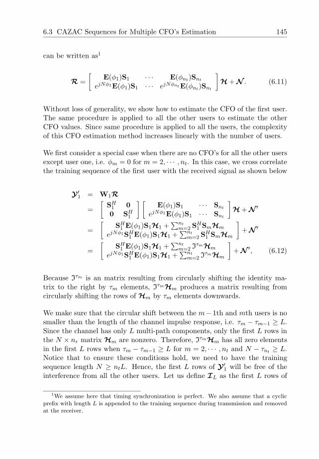
6.3 CAZAC Sequences for Multiple CFO’s Estimation 145
can be written as1
R =[
E(φ1)S1 · · · E(φnt)Snt
ejNφ1E(φ1)S1 · · · ejNφntE(φnt)Snt
]H + N . (6.11)
Without loss of generality, we show how to estimate the CFO of the first user.The same procedure is applied to all the other users to estimate the otherCFO values. Since same procedure is applied to all the users, the complexityof this CFO estimation method increases linearly with the number of users.
We first consider a special case when there are no CFO’s for all the other usersexcept user one, i.e. φm = 0 for m = 2, · · · , nt. In this case, we cross correlatethe training sequence of the first user with the received signal as shown below
Y ′1 = W1R
=[
SH1 00 SH
1
] [E(φ1)S1 · · · Snt
ejNφ1E(φ1)S1 · · · Snt
]H + N ′
=[
SH1 E(φ1)S1H1 +
∑ntm=2 SH
1 SmHm
ejNφ1SH1 E(φ1)S1H1 +
∑ntm=2 SH
1 SmHm
]+ N ′
=[
SH1 E(φ1)S1H1 +
∑ntm=2 IτmHm
ejNφ1SH1 E(φ1)S1H1 +
∑ntm=2 IτmHm
]+ N ′, (6.12)
Because Iτm is an matrix resulting from circularly shifting the identity ma-trix to the right by τm elements, IτmHm produces a matrix resulting fromcircularly shifting the rows of Hm by τm elements downwards.
We make sure that the circular shift between the m− 1th and mth users is nosmaller than the length of the channel impulse response, i.e. τm − τm−1 ≥ L.Since the channel has only L multi-path components, only the first L rows inthe N × nr matrix Hm are nonzero. Therefore, IτmHm has all zero elementsin the first L rows when τm − τm−1 ≥ L for m = 2, · · · , nt and N − τnt ≥ L.Notice that to ensure these conditions hold, we need to have the trainingsequence length N ≥ ntL. Hence, the first L rows of Y ′
1 will be free of theinterference from all the other users. Let us define IL as the first L rows of
1We assume here that timing synchronization is perfect. We also assume that a cyclicprefix with length L is appended to the training sequence during transmission and removedat the receiver.
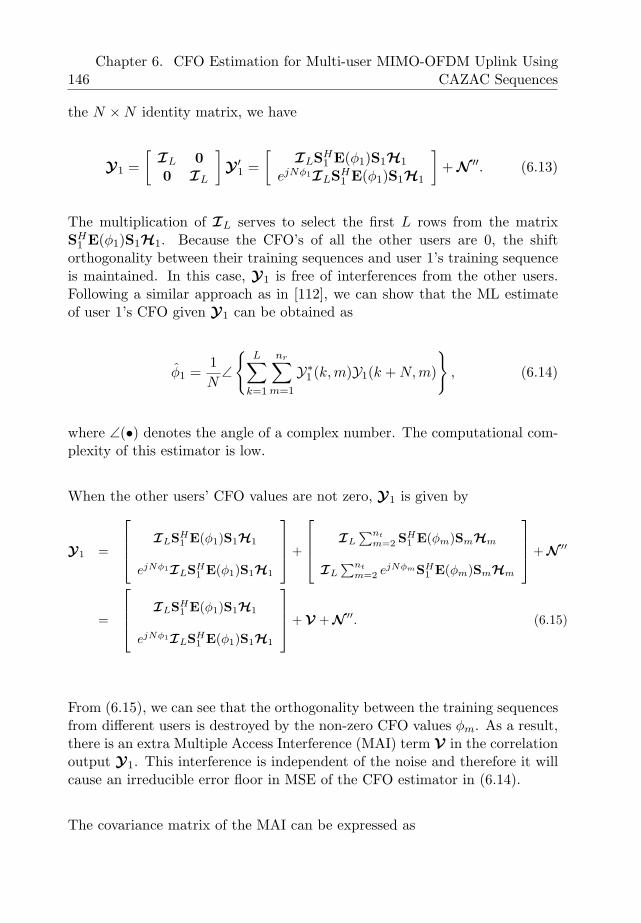
146Chapter 6. CFO Estimation for Multi-user MIMO-OFDM Uplink Using
CAZAC Sequences
the N ×N identity matrix, we have
Y1 =[ IL 0
0 IL
]Y ′
1 =[ ILSH
1 E(φ1)S1H1
ejNφ1ILSH1 E(φ1)S1H1
]+ N ′′. (6.13)
The multiplication of IL serves to select the first L rows from the matrixSH
1 E(φ1)S1H1. Because the CFO’s of all the other users are 0, the shiftorthogonality between their training sequences and user 1’s training sequenceis maintained. In this case, Y1 is free of interferences from the other users.Following a similar approach as in [112], we can show that the ML estimateof user 1’s CFO given Y1 can be obtained as
φ1 =1N
∠
L∑
k=1
nr∑
m=1
Y∗1 (k, m)Y1(k + N, m)
, (6.14)
where ∠(•) denotes the angle of a complex number. The computational com-plexity of this estimator is low.
When the other users’ CFO values are not zero, Y1 is given by
Y1 =
ILSH1 E(φ1)S1H1
ejNφ1ILSH1 E(φ1)S1H1
+
IL
∑nt
m=2 SH1 E(φm)SmHm
IL
∑nt
m=2 ejNφmSH1 E(φm)SmHm
+ N ′′
=
ILSH1 E(φ1)S1H1
ejNφ1ILSH1 E(φ1)S1H1
+ V + N ′′. (6.15)
From (6.15), we can see that the orthogonality between the training sequencesfrom different users is destroyed by the non-zero CFO values φm. As a result,there is an extra Multiple Access Interference (MAI) term V in the correlationoutput Y1. This interference is independent of the noise and therefore it willcause an irreducible error floor in MSE of the CFO estimator in (6.14).
The covariance matrix of the MAI can be expressed as
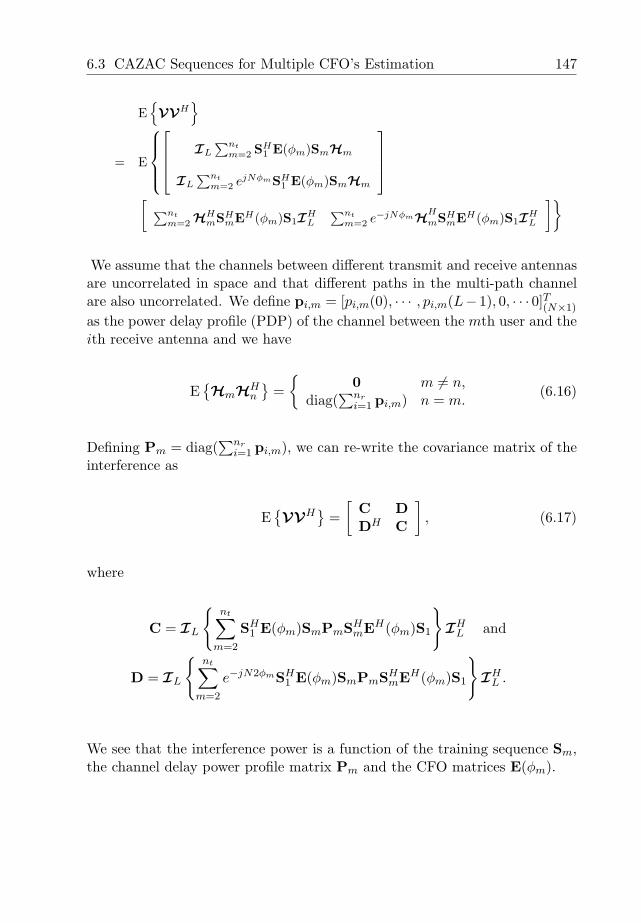
6.3 CAZAC Sequences for Multiple CFO’s Estimation 147
E
VVH
= E
IL
∑nt
m=2 SH1 E(φm)SmHm
IL
∑nt
m=2 ejNφmSH1 E(φm)SmHm
[∑nt
m=2 HHmSH
mEH(φm)S1IHL
∑nt
m=2 e−jNφmHHmSH
mEH(φm)S1IHL
]
We assume that the channels between different transmit and receive antennasare uncorrelated in space and that different paths in the multi-path channelare also uncorrelated. We define pi,m = [pi,m(0), · · · , pi,m(L− 1), 0, · · · 0]T(N×1)
as the power delay profile (PDP) of the channel between the mth user and theith receive antenna and we have
EHmHH
n
=
0 m 6= n,
diag(∑nr
i=1 pi,m) n = m.(6.16)
Defining Pm = diag(∑nr
i=1 pi,m), we can re-write the covariance matrix of theinterference as
EVVH
=
[C DDH C
], (6.17)
where
C = IL
nt∑
m=2
SH1 E(φm)SmPmSH
mEH(φm)S1
IH
L and
D = IL
nt∑
m=2
e−jN2φmSH1 E(φm)SmPmSH
mEH(φm)S1
IH
L .
We see that the interference power is a function of the training sequence Sm,the channel delay power profile matrix Pm and the CFO matrices E(φm).
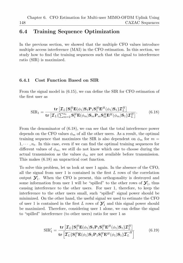
148Chapter 6. CFO Estimation for Multi-user MIMO-OFDM Uplink Using
CAZAC Sequences
6.4 Training Sequence Optimization
In the previous section, we showed that the multiple CFO values introducemultiple access interference (MAI) in the CFO estimation. In this section, westudy how to find the training sequences such that the signal to interferenceratio (SIR) is maximized.
6.4.1 Cost Function Based on SIR
From the signal model in (6.15), we can define the SIR for CFO estimation ofthe first user as
SIR1 =tr
[ILSH1 E(φ1)S1P1SH
1 EH(φ1)S1IHL
]
tr[IL
∑ntm=2 SH
1 E(φm)SmPmSHmEH(φm)S1IH
L
] . (6.18)
From the denominator of (6.18), we can see that the total interference powerdepends on the CFO values φm of all the other users. As a result, the optimaltraining sequence that maximizes the SIR is also dependent on φm for m =1, · · · , nt. In this case, even if we can find the optimal training sequences fordifferent values of φm, we still do not know which one to choose during theactual transmission as the values φm are not available before transmission.This makes (6.18) an unpractical cost function.
To solve this problem, let us look at user 1 again. In the absence of the CFO,all the signal from user 1 is contained in the first L rows of the correlationoutput Y ′
1. When the CFO is present, this orthogonality is destroyed andsome information from user 1 will be “spilled” to the other rows of Y ′
1, thuscausing interference to the other users. For user 1, therefore, to keep theinterference to the other users small, such “spilled” signal power should beminimized. On the other hand, the useful signal we used to estimate the CFOof user 1 is contained in the first L rows of Y ′
1 and this signal power shouldbe maximized. Therefore, considering user 1 alone, we can define the signalto “spilled” interference (to other users) ratio for user 1 as
SIR′1 =tr
[ILSH1 E(φ1)S1P1SH
1 EH(φ1)S1IHL
]
tr[ILSH
1 E(φ1)S1P1SH1 EH(φ1)S1IL
H] (6.19)
6.4 Training Sequence Optimization 149
where IL is the complement of IL, i.e. IL is the last N−L rows of the N×Nidentity matrix.
The denominator in (6.19) can be expressed as
tr[ILSH
1 E(φ1)S1P1SH1 EH(φ1)S1IL
H]
= Ntr[S1P1SH
1
]− tr[ILSH
1 E(φ1)S1P1SH1 EH(φ1)S1IL
H]
= N2tr [P1]− tr[ILSH
1 E(φ1)S1P1SH1 EH(φ1)S1IL
H].
Substituting this into (6.19), we have
SIR′1 =tr
[ILSH1 E(φ1)S1P1SH
1 EH(φ1)S1IHL
]
N2tr[P1]− tr[ILSH
1 E(φ1)S1P1SH1 EH(φ1)S1IH
L
] .
(6.20)
Now we can define the training sequence optimization problem as
Sopt = arg maxS1
SIR′1
= arg maxS1
tr[ILSH
1 E(φ1)S1P1SH1 EH(φ1)S1IH
L
]
N2tr[P1]− tr[ILSH
1 E(φ1)S1P1SH1 EH(φ1)S1IH
L
]
= arg minS1
N2tr[P1]− tr[ILSH
1 E(φ1)S1P1SH1 EH(φ1)S1IH
L
]
tr[ILSH
1 E(φ1)S1P1SH1 EH(φ1)S1IH
L
]
= arg minS1
N2tr[P1]
tr[ILSH
1 E(φ1)S1P1SH1 EH(φ1)S1IH
L
] − 1
= arg maxS1
tr
[ILSH
1 E(φ1)S1P1SH1 EH(φ1)S1IH
L
]. (6.21)
From (6.21), we can see that the optimal training sequence depends on thepower delay profile P1 and the actual CFO value φ1. The channel delay profileis an environment-dependent statistical property that does not change very
150Chapter 6. CFO Estimation for Multi-user MIMO-OFDM Uplink Using
CAZAC Sequences
frequently. Therefore, in practice, we can store a few training sequences fordifferent typical power delay profiles at the transmitter and select the one thatmatches the actual channel delay profile. On the other hand, it is impossibleto know the actual CFO φ in advance to select the optimal training sequence.Next, we will propose a new cost function based on SIR approximation whichcan remove the dependency on the actual CFO φ1 in the optimization.
6.4.2 CFO-Independent Cost Function
Let us assume that the CFO value φ is small. In this case, we can approximatethe exponential function in the original cost function by its first-order Taylorseries expansion, i.e. exp(jφ) ≈ 1 + jφ. Therefore, we have
E(φ1) ≈ IN + jφ1N, (6.22)
where N is a diagonal matrix given by N =diag[0, 1, 2, · · · , N − 1]. Using thisapproximation, we get
SHE(φ)SPSHEH(φ)S ≈ SH(I + jφN)SPSH(I− jφN)S= P + jφSHNSP− jφPSHNS + φ2SHNSPSHNS.
(6.23)
Here we omitted the subscript 1 for clearness of presentation. Therefore, theoptimization problem can be approximated as
Sopt = arg maxS
tr
[IL
(P + jφSHNSP− jφPS
HNS + φ2SHNSPS
HNS
)IH
L
].
(6.24)
Notice that the first term P in the summation is independent of S and hencecan be dropped. It can be shown that the diagonal elements of the second termjφSHNSP are constant and independent of S. Therefore tr
[IL(jφSHNSP)IH
L
]
is also independent of S and hence can be dropped from the cost function. Thesame applies to the third term −jφPS
HNS, which is the conjugate of the sec-
ond term. Therefore, the final form of the optimization using Taylor’s series
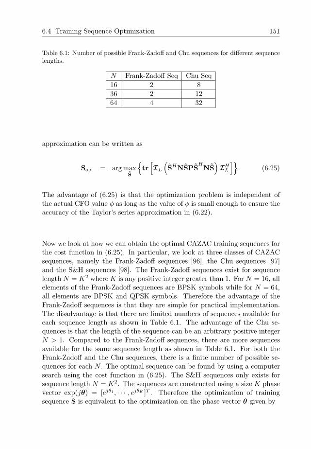
6.4 Training Sequence Optimization 151
Table 6.1: Number of possible Frank-Zadoff and Chu sequences for different sequencelengths.
N Frank-Zadoff Seq Chu Seq16 2 836 2 1264 4 32
approximation can be written as
Sopt = arg maxS
tr
[IL
(SHNSPS
HNS
)IH
L
]. (6.25)
The advantage of (6.25) is that the optimization problem is independent ofthe actual CFO value φ as long as the value of φ is small enough to ensure theaccuracy of the Taylor’s series approximation in (6.22).
Now we look at how we can obtain the optimal CAZAC training sequences forthe cost function in (6.25). In particular, we look at three classes of CAZACsequences, namely the Frank-Zadoff sequences [96], the Chu sequences [97]and the S&H sequences [98]. The Frank-Zadoff sequences exist for sequencelength N = K2 where K is any positive integer greater than 1. For N = 16, allelements of the Frank-Zadoff sequences are BPSK symbols while for N = 64,all elements are BPSK and QPSK symbols. Therefore the advantage of theFrank-Zadoff sequences is that they are simple for practical implementation.The disadvantage is that there are limited numbers of sequences available foreach sequence length as shown in Table 6.1. The advantage of the Chu se-quences is that the length of the sequence can be an arbitrary positive integerN > 1. Compared to the Frank-Zadoff sequences, there are more sequencesavailable for the same sequence length as shown in Table 6.1. For both theFrank-Zadoff and the Chu sequences, there is a finite number of possible se-quences for each N . The optimal sequence can be found by using a computersearch using the cost function in (6.25). The S&H sequences only exists forsequence length N = K2. The sequences are constructed using a size K phasevector exp(jθ) = [ejθ1 , · · · , ejθK ]T . Therefore the optimization of trainingsequence S is equivalent to the optimization on the phase vector θ given by
152Chapter 6. CFO Estimation for Multi-user MIMO-OFDM Uplink Using
CAZAC Sequences
θ = arg maxθ
J (θ)
with
J (θ) = tr[IL
(SH(θ)NS(θ)PS
H(θ)NS(θ)
)IH
L
]. (6.26)
Notice that each element of the phase vector can take any values in the interval[0, 2π). From the construction of the S&H sequence [98], it can be easily showthat S(θ + ψ) = ejψS(θ), where θ + ψ = [θ1 + ψ, · · · , θK + ψ]T . Hence,from (6.26), we can get J (θ) = J (θ + ψ). By letting ψ = −θ1, the originaloptimization problem over the K-dimension phase vector θ = [θ1, θ2, · · · , θK ]T
can be simplified to the optimization over a (K − 1)-dimension phase vectorθ′ = [0, θ′1, · · · , θ′K−1]
T where θ′k = θk+1 − θ1.
Since there is an infinite number of possible S&H sequences for each sequencelength, it is impossible to use exhaustive computer search to obtain the opti-mal sequence. We resort to numerical methods and use the adaptive simulatedannealing (ASA) method [110] to find a near-optimal sequence. To test thenear-optimality of the sequence obtained using the ASA, for smaller sequencelengths of N = 16 and N = 36, we use exhaustive computer search to ob-tain the globally optimal S&H sequence 2. The obtained sequence throughcomputer search is consistent with the sequence obtained using ASA and thissuggests the effectiveness of the ASA in approaching the globally optimal se-quence.
6.5 Simulation Results
In this section, we use computer simulations to study the performance of theCFO estimation using CAZAC sequences and demonstrate the performancegain achieved by using optimal training sequences. In the simulations, weassume a multi-user MIMO-OFDM systems with two users. Each user hasone transmit antenna and the base station has two receive antennas. We
2Because CFO values are continuous variables, strictly speaking, it is not possible toobtain the exact optimum using exhaustive computer search, because the search works withdiscrete variables. If we keep the step size in the search small enough, we can be sure thatthe obtained ”optimum” is very close to the actual optimum and can be practically assumedto be the actual optimum.
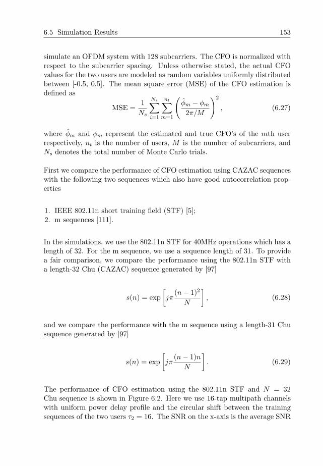
6.5 Simulation Results 153
simulate an OFDM system with 128 subcarriers. The CFO is normalized withrespect to the subcarrier spacing. Unless otherwise stated, the actual CFOvalues for the two users are modeled as random variables uniformly distributedbetween [-0.5, 0.5]. The mean square error (MSE) of the CFO estimation isdefined as
MSE =1
Ns
Ns∑
i=1
nt∑
m=1
(φm − φm
2π/M
)2
, (6.27)
where φm and φm represent the estimated and true CFO’s of the mth userrespectively, nt is the number of users, M is the number of subcarriers, andNs denotes the total number of Monte Carlo trials.
First we compare the performance of CFO estimation using CAZAC sequenceswith the following two sequences which also have good autocorrelation prop-erties
1. IEEE 802.11n short training field (STF) [5];2. m sequences [111].
In the simulations, we use the 802.11n STF for 40MHz operations which has alength of 32. For the m sequence, we use a sequence length of 31. To providea fair comparison, we compare the performance using the 802.11n STF witha length-32 Chu (CAZAC) sequence generated by [97]
s(n) = exp[jπ
(n− 1)2
N
], (6.28)
and we compare the performance with the m sequence using a length-31 Chusequence generated by [97]
s(n) = exp[jπ
(n− 1)nN
]. (6.29)
The performance of CFO estimation using the 802.11n STF and N = 32Chu sequence is shown in Figure 6.2. Here we use 16-tap multipath channelswith uniform power delay profile and the circular shift between the trainingsequences of the two users τ2 = 16. The SNR on the x-axis is the average SNR
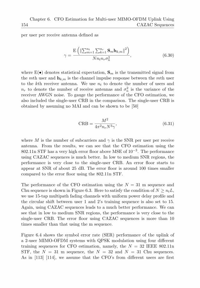
154Chapter 6. CFO Estimation for Multi-user MIMO-OFDM Uplink Using
CAZAC Sequences
per user per receive antenna defined as
γ =E
(‖∑nt
m=1
∑nrk=1 Smhk,m‖2
)
Nntnrσ2n
, (6.30)
where E(•) denotes statistical expectation, Sm is the transmitted signal fromthe mth user and hk,m is the channel impulse response between the mth userto the kth receiver antenna. We use nt to denote the number of users andnr to denote the number of receive antennas and σ2
n is the variance of thereceiver AWGN noise. To gauge the performance of the CFO estimation, wealso included the single-user CRB in the comparison. The single-user CRB isobtained by assuming no MAI and can be shown to be [50]
CRB =M2
4π2nrN3γ, (6.31)
where M is the number of subcarriers and γ is the SNR per user per receiveantenna. From the results, we can see that the CFO estimation using the802.11n STF has a very high error floor above MSE of 10−3. The performanceusing CAZAC sequences is much better. In low to medium SNR regions, theperformance is very close to the single-user CRB. An error floor starts toappear at SNR of about 25 dB. The error floor is around 100 times smallercompared to the error floor using the 802.11n STF.
The performance of the CFO estimation using the N = 31 m sequence andChu sequence is shown in Figure 6.3. Here to satisfy the condition of N ≥ ntL,we use 15-tap multipath fading channels with uniform power delay profile andthe circular shift between user 1 and 2’s training sequence is also set to 15.Again, using CAZAC sequences leads to a much better performance. We cansee that in low to medium SNR regions, the performance is very close to thesingle-user CRB. The error floor using CAZAC sequences is more than 10times smaller than that using the m sequence.
Figure 6.4 shows the symbol error rate (SER) performance of the uplink ofa 2-user MIMO-OFDM systems with QPSK modulation using four differenttraining sequences for CFO estimation, namely, the N = 32 IEEE 802.11nSTF, the N = 31 m sequence, the N = 32 and N = 31 Chu sequences.As in [113] [114], we assume that the CFO’s from different users are first
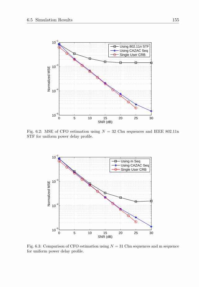
6.5 Simulation Results 155
0 5 10 15 20 25 3010
−5
10−4
10−3
10−2
SNR (dB)
Nor
mal
ized
MS
E
Using 802.11n STFUsing CAZAC SeqSingle User CRB
Fig. 6.2: MSE of CFO estimation using N = 32 Chu sequences and IEEE 802.11nSTF for uniform power delay profile.
0 5 10 15 20 25 3010
−5
10−4
10−3
10−2
SNR (dB)
Nor
mal
ized
MS
E
Using m SeqUsing CAZAC SeqSingle User CRB
Fig. 6.3: Comparison of CFO estimation using N = 31 Chu sequences and m sequencefor uniform power delay profile.
156Chapter 6. CFO Estimation for Multi-user MIMO-OFDM Uplink Using
CAZAC Sequences
5 10 15 20 25 30 35
10−4
10−3
10−2
10−1
100
SNR (dB)
SE
R
No CFO EstCFO Est Using N=32 11n STFCFO Est Using N=31 m seqCFO Est using N=32 Chu seqCFO Est using N=31 Chu seqPerf. CFO Est
Fig. 6.4: Comparison of SER using QPSK modulation for CFO estimation usingdifferent sequences for uniform power delay profile.
estimated at the base station using the proposed algorithm and transmittedback to different users using a downlink control channel. These CFO’s arepre-compensated at each user’s transmitter and the SER is measured at thereceiver for this transmission. We assume perfect channel knowledge at thereceiver and linear minimum mean square error (LMMSE) detection is used.We can see that the system fails if there is no CFO estimation. Due to thehigh error floor in the CFO estimation using the IEEE 802.11n STF, the SERperformance is very poor. The performance using m sequence is better and hasan error floor at SER of 0.002. The performance using the two Chu sequencesdoes not have any error floor and is very close to the performance of perfectCFO estimation for SNR above 15 dB.
The performance of CFO estimation using different CAZAC sequences is com-pared in Figure 6.5. Here we fix the sequence length to 36 and the multi-pathchannel has L = 18 taps with uniform power delay profile. Comparing theperformances of the optimal Chu sequence and the optimal Frank-Zadoff se-quence, we can see that the error floor of the Chu sequence is smaller. Thisis because there are more possible Chu sequences compared to Frank-Zadoffsequences and hence more degrees of freedom in the optimization. However,comparing the performance of the optimal Chu sequence with that of the op-timal S&H sequences, we can see that the additional degrees of freedom in the
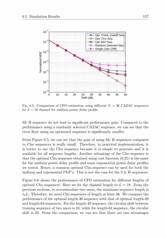
6.5 Simulation Results 157
5 10 15 20 25 30 35 40 45 5010
−8
10−7
10−6
10−5
10−4
10−3
10−2
SNR (dB)
Nor
mal
ized
MS
E
Opt. Frank−Zadoff SeqOpt. Chu SeqOpt S&H SeqRandom Selected SeqSingle User CRB
Fig. 6.5: Comparison of CFO estimation using different N = 36 CAZAC sequencesfor L = 18 channel for uniform power delay profile.
S& H sequence do not lead to significant performance gain. Compared to theperformance using a randomly selected CAZAC sequence, we can see that theerror floor using an optimized sequence is significantly smaller.
From Figure 6.5, we can see that the gain of using S& H sequences comparedto Chu sequences is really small. Therefore, in practical implementation, itis better to use the Chu sequence because it is simple to generate and it isavailable for all sequence lengths. Another advantage of the Chu sequence isthat the optimal Chu sequence obtained using cost function (6.25) is the samefor the uniform power delay profile and some exponential power delay profileswe tested. Hence, a common optimal Chu sequence can be used for both theuniform and exponential PDP’s. This is not the case for the S & H sequences.
Figure 6.6 shows the performance of CFO estimation for different lengths ofoptimal Chu sequences. Here we fix the channel length to L = 18. From theprevious sections, to accommodate two users, the minimum sequence length isntL. Therefore, we need Chu sequences of length at least 36. We compare theperformance of the optimal length-36 sequence with that of optimal length-49and length-64 sequences. For the length-49 sequence, the circular shift betweentraining sequence of two users is 24, while for length-64 sequence, the circularshift is 32. From the comparison, we can see that there are two advantages
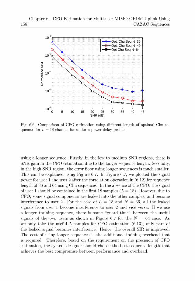
158Chapter 6. CFO Estimation for Multi-user MIMO-OFDM Uplink Using
CAZAC Sequences
0 5 10 15 20 25 30 35 40 4510
−6
10−5
10−4
10−3
10−2
SNR (dB)
Nor
mal
ized
MS
E
Opt. Chu Seq N=36Opt. Chu Seq N=49Opt Chu Seq N=64
Fig. 6.6: Comparison of CFO estimation using different length of optimal Chu se-quences for L = 18 channel for uniform power delay profile.
using a longer sequence. Firstly, in the low to medium SNR regions, there isSNR gain in the CFO estimation due to the longer sequence length. Secondly,in the high SNR region, the error floor using longer sequences is much smaller.This can be explained using Figure 6.7. In Figure 6.7, we plotted the signalpower for user 1 and user 2 after the correlation operation in (6.12) for sequencelength of 36 and 64 using Chu sequences. In the absence of the CFO, the signalof user 1 should be contained in the first 18 samples (L = 18). However, due toCFO, some signal components are leaked into the other samples, and becomeinterference to user 2. For the case of L = 18 and N = 36, all the leakedsignals from user 1 become interference to user 2 and vice versa. If we usea longer training sequence, there is some “guard time” between the usefulsignals of the two users as shown in Figure 6.7 for the N = 64 case. Aswe only take the useful L samples for CFO estimation (6.13), only part ofthe leaked signal becomes interference. Hence, the overall SIR is improved.The cost of using longer sequences is the additional training overhead thatis required. Therefore, based on the requirement on the precision of CFOestimation, the system designer should choose the best sequence length thatachieves the best compromise between performance and overhead.
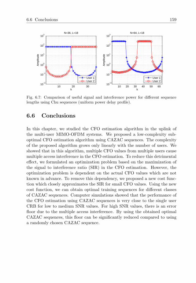
6.6 Conclusions 159
10 20 3010
−2
10−1
100
101
102
103
k
Am
plitu
de
N=36, L=18
User 1User 2
10 20 30 40 50 6010
−2
10−1
100
101
102
103
k
Am
plitu
de
N=64, L=18
User 1User 2
Fig. 6.7: Comparison of useful signal and interference power for different sequencelengths using Chu sequences (uniform power delay profile).
6.6 Conclusions
In this chapter, we studied the CFO estimation algorithm in the uplink ofthe multi-user MIMO-OFDM systems. We proposed a low-complexity sub-optimal CFO estimation algorithm using CAZAC sequences. The complexityof the proposed algorithm grows only linearly with the number of users. Weshowed that in this algorithm, multiple CFO values from multiple users causemultiple access interference in the CFO estimation. To reduce this detrimentaleffect, we formulated an optimization problem based on the maximization ofthe signal to interference ratio (SIR) in the CFO estimation. However, theoptimization problem is dependent on the actual CFO values which are notknown in advance. To remove this dependency, we proposed a new cost func-tion which closely approximates the SIR for small CFO values. Using the newcost function, we can obtain optimal training sequences for different classesof CAZAC sequences. Computer simulations showed that the performance ofthe CFO estimation using CAZAC sequences is very close to the single userCRB for low to medium SNR values. For high SNR values, there is an errorfloor due to the multiple access interference. By using the obtained optimalCAZAC sequences, this floor can be significantly reduced compared to usinga randomly chosen CAZAC sequence.

160Chapter 6. CFO Estimation for Multi-user MIMO-OFDM Uplink Using
CAZAC Sequences
Chapter 7Conclusions and Future Work
7.1 Conclusions
Sensitivity to carrier frequency offset (CFO) is a major drawback of orthogo-nal frequency division multiplexing (OFDM) systems. In this thesis, we studylow-complexity frequency synchronization techniques that can accurately esti-mate the CFO for wireless OFDM systems. The focus is on finding frequencysynchronization techniques that achieve a good balance between performanceand computational complexity. We developed CFO estimation algorithms forvarious wireless OFDM systems that can be implemented with low complexity,and at the same time achieve close to maximum-likelihood (ML) or Cramer-Rao Bound (CRB) performance for practical CFO values.
In Chapters 2 and 3 of the thesis, we studied low-complexity blind CFO esti-mation algorithms that exploit frequency-domain null subcarriers, which aresubcarriers that are left empty. Existing algorithms of this type have a highcomputational complexity because the cost function of CFO estimation is ahigh-order polynomial and a search method is needed to find the CFO esti-mate. By using a low-order Taylor series approximation of the cost function,we derived a closed-form solution for the CFO estimate. We also developeda new factorization of the cost function such that the error between the orig-inal cost function and the low-order Taylor series approximation is reduced.
162 Chapter 7. Conclusions and Future Work
We noticed that when the CFO is large, the approximation error still causessome performance degradation in CFO estimation especially in the high SNRregion. To reduce this degradation, we further developed a successive algo-rithm, in which the CFO is estimated and compensated successively in severaliterations. A convergence monitoring method was implemented to ensure thatthe CFO obtained using the successive algorithm converges to the same CFOobtained using the high-complexity search method. We showed using com-puter simulations that the proposed successive algorithm achieves the sameperformance as the search method in 2 to 3 iterations. The computationalcomplexity of the developed algorithm is significantly lower than that usingthe search method. In the literature, it was shown that the CRB of the CFOestimation is minimized if the null subcarriers are placed with equal spacing inan OFDM symbol. In our study in Chapter 3, we found that the signal to noiseratio (SNR) of the CFO estimation is related to the null subcarrier placement.To gain additional insight on the best null subcarrier placement, we studiedthe null subcarrier placement that maximizes this SNR. For small CFO val-ues, we showed that this optimization problem is convex and the SNR of theCFO estimation is maximized when the null subcarriers are evenly spaced.This is consistent with the null subcarrier placement that minimizes the CRB.However, when the number of subcarriers is not divisible by the number ofnull subcarriers, it is not possible to place null subcarriers with even spac-ing. To solve this practical problem, we proposed a heuristic null subcarrierplacement, which still leads to good performance in the CFO estimation. Forpractical OFDM systems where two guard bands are required at both ends ofthe spectrum, we showed that by placing a few null subcarriers optimally in-side the data band, the performance of the CFO estimation can be significantlyimproved.
In Chapters 4 and 5, we studied frequency synchronization for multiple inputmultiple output (MIMO) OFDM systems. In MIMO systems, there are mul-tiple front-ends at both the transmitter and the receiver. As a result, thereare different clock signal generation and distribution topologies specifying howclock signals are generated and distributed to different front-ends. In Chapter4, we presented a study on the power dissipations of three commonly usedtopologies. We first developed a general system model to calculate the powerdissipations for different topologies. We then presented a case study on thepower dissipations of a MIMO receiver with 4 antennas in the 2.4 GHz, 5 GHzand 60 GHz bands using different clock signal generation and distributiontopologies. The results showed that, because of the high power dissipationof the frequency synthesizer, the centralized clock signal generation, whereonly one frequency synthesizer is used, consumes less power compared to dis-
7.1 Conclusions 163
tributed clock signal generation. On the other hand, distributed clock gener-ation topologies have the potential to reduce the complexity and cost of thereceiver front-end because there are no GHz RF signals distributed in the sys-tem. In Chapter 5, we proposed an efficient training sequence design for jointCFO and channel estimation in MIMO-OFDM systems using centralized clocksignal generation and distribution. We showed that using the proposed train-ing sequence, the ML CFO and channel estimates can be obtained with lowcomputational complexity. The training overhead is also significantly lowerthan for the conventional frequency-domain training sequence. Moreover, wederived an accurate closed-form approximation of the performance of channelestimation in the presence of residual CFO. In Chapter 5, we also studied theeffects of spatial correlation and antenna mutual coupling on the performanceof CFO estimation in MIMO systems. We showed that spatial correlation de-grades the performance of CFO estimation. Antenna mutual coupling has twoeffects. Firstly, it reduces spatial correlation, which is beneficial. Secondlyit also reduces the power of the received signal, which is detrimental. Com-puter simulations showed that the combined effect of mutual coupling addsadditional degradation to the CFO estimation performance.
In Chapter 6, we studied the frequency synchronization in the uplink of multi-user MIMO-OFDM systems. We proposed a low-complexity CFO estimationalgorithm using constant amplitude zero autocorrelation (CAZAC) trainingsequences. We showed that using the proposed algorithm, the CFO estimatesof different users can be obtained using simple correlation operations. Thecomputational complexity of the proposed algorithm is much lower than ex-isting algorithms in the literature, while the performance is close to optimum.Moreover, the computational complexity of the proposed algorithm only growslinearly with the number of users. However, we showed that multiple CFO’scause multiple access interference (MAI) in the CFO estimation of differentusers using the proposed low-complexity algorithm. This leads to an errorfloor in the mean square error (MSE) of the CFO estimates. To reduce thisdegradation, we formulated an optimization problem to find the training se-quences that maximize the signal to multiple access interference ratio (SIR).However, the optimal training sequences depend on the actual CFO values,which are not known in advance. To solve this problem, we developed a newcost function that closely approximates the SIR for small CFO values and isindependent of the actual CFO values. We showed using computer simula-tions that the performance of CFO estimation using the proposed CAZACsequences reaches the single user CRB for low to medium SNR regions. Byusing the proposed optimal CAZAC sequence, the error floor in the high SNRregion is much lower than for a randomly selected CAZAC sequence.
164 Chapter 7. Conclusions and Future Work
7.2 Future Work
In this section, we would like to make the following recommendations on thepossible future work based on the research carried out in this thesis.
• In practical wireless OFDM systems, it is usually required by industrialstandards to have guard bands at both ends of the spectrum to avoid alias-ing to the adjacent bands and also to avoid interference from the adjacentbands. In this case, the frequency responses of training sequences on thesubcarriers in the guard bands are required to be zero. We did not considerthis constraint, which must be satisfied in a practical OFDM system, in thedesign of CAZAC training sequences in MIMO-OFDM systems. Therefore,it is of practical importance to investigate whether there are CAZAC se-quences that satisfy this constraint. If not, then it would be interesting tosee what other sequences we should use and how to construct and optimizethem. In designing a good training sequence with the guard band con-straint, we believe there is a trade-off between small guard band responseand small auto-correlation of the sequence. Therefore, it is interesting toinvestigate how we can formulate this trade-off and find a good practicaltraining sequence. Moreover, the constant amplitude requirement on theCAZAC training sequence is not essential as long as the peak to averagepower ratio (PAPR) of the training sequence is reasonably small. Thus, wecan relax the constant amplitude constraint in the training sequence design,which gives us additional degrees of freedom.
• Due to time constraints, in this thesis, we did not consider channel estima-tion for different users in the uplink of multi-user MIMO-OFDM systemsusing CAZAC sequences. It is worthwhile to study the joint CFO andchannel estimation and the effect of residual CFO on the channel estima-tion in the multi-user systems. This study will aid us in the design of asingle training sequence for joint CFO and channel estimation in the up-link of multi-user MIMO-OFDM systems. Moreover, a comparison withthe results obtained in Chapter 5 for single-user MIMO-OFDM systemscan provide us with additional insights on the training sequence design formulti-user systems.
• In Chapter 6, when we studied the symbol error rate (SER) performancein the uplink of multi-user MIMO-OFDM systems, we assumed there is adownlink control link, using which the CFO values for different users are sentback to the transmitter and pre-compensated. It is an interesting problemto study how CFO compensation can be performed at the receiver. In thiscase, the communication of the CFO values back to the transmitter is not
7.2 Future Work 165
necessary and the system design can be simplified significantly. However,the CFO compensation in a multi-user receiver is not trivial, as compensat-ing one user’s CFO might worsen the CFO of another user. If CFO’s canbe successfully compensated with low complexity, we can re-estimate theresidual CFO’s using the compensated received signal and obtain a betterCFO estimates. This is because the multiple access interference (MAI) forthe CFO estimation in multi-user MIMO-OFDM systems is directly relatedto the amplitude of the CFO. If the initial CFO’s are estimated with suf-ficient accuracy, after CFO compensation, the residual CFO’s are smallerthan the initial CFO and hence introduce less MAI. Therefore, the residualCFO’s can be estimated with better accuracy. In this way, we can re-usethe successive CFO estimation and compensation algorithm developed inChapter 2 in the uplink multi-user MIMO-OFDM systems to improve theperformance of the CFO estimation.
• Recently, cooperative wireless communication has become a hot researchtopic. In a cooperative wireless communication system, different wirelessnodes in a communication network cooperate to enhance the quality of thecommunication link between any two nodes. There are many papers in theliterature focusing on transmission strategies to maximize the link through-put or minimize the bit error rate of the transmission. Most of these papersassume perfect timing and frequency synchronization. In practice, bothtiming and frequency synchronization in cooperative communication sys-tems are difficult due to the distributed nature of the wireless nodes andalso the potentially large number of nodes in the network. Due to this dif-ficulty, many transmission strategies have been designed considering onlyasynchronous communication, which has inferior performance compared toa fully synchronized system. Since the algorithms we proposed in Chap-ter 6 are targeted to multi-user communication systems, it is interestingto investigate their applicability in and possible extensions to cooperativecommunication systems.

166 Chapter 7. Conclusions and Future Work
Bibliography
[1] T. S. Rappaport, Wireless communications principles & practice. Pren-tice Hall Inc., 1996.
[2] W. Jakes, Microwave mobile communications. IEEE Press, 1994.
[3] J. G. Proakis, Digital communications, 4th ed. McGraw-Hill, 2001.
[4] IEEE 802.11b-1999 Higher Speed Physical Layer Extension in the 2.4GHz band, IEEE Std., Feb. 1999.
[5] IEEE P802.11n/D1.10 Wireless LAN Medium Access Control (MAC)and Physical Layer (PHY) specifications: Enhancements for HigherThroughput, IEEE Std., Feb 2007.
[6] E. Perahia, “IEEE P802.11 Wireless LANs VHT 60 GHz PAR plus5C’s,” IEEE 802.11 document IEEE 802.11-08/0806r7, Oct. 2008.
[7] S. Cherry, “Edholm’s law of bandwidth,” IEEE Spectr., vol. 41, no. 7,pp. 58–60, July 2004.
[8] G. Moore, “Cramming more components onto integrated circuits,” Elec-tronics, vol. 38, no. 8, April 1965.
[9] E. A. Lee and D. G. Messerschnitt, Digital communication, 2nd ed.Kluwer Academic Publishers, 1999.
[10] S. Haykin, Adaptive filter theory, 4th ed. Prentice Hall Inc., 2002.
[11] R. Prasad, OFDM for wireless communications systems. Artech HouseInc., 2004.
168 Bibliography
[12] R. Chang, “Synthesis of band-limited orthogonal signals for multi-channel data transmission,” Bell Syst. Tech. Journal, vol. 45, pp. 1775–1796, Dec 1966.
[13] B. Saltzberg, “Performance of an efficient parallel data transmission sys-tem,” IEEE Trans. Commun. Technol., vol. 15, no. 6, pp. 805–811, De-cember 1967.
[14] J. A. C. Bingham, “Multicarrier modulation for data transmission: anidea whose time has come,” IEEE Commun. Mag., vol. 28, no. 5, pp.5–14, May 1990.
[15] J. M. Cioffi, “A multicarrier primer,” ANSI TlEl.4 Committee Contri-bution, pp. 91–157, Nov. 1991.
[16] W. Y. Zou and Y. Wu, “COFDM: an overview,” IEEE Trans. Broadcast.,vol. 41, no. 1, pp. 1–8, March 1995.
[17] IEEE 802.11a: Wireless LAN Medium Access Control (MAC) and Phys-ical Layer (PHY) Specifications: High-speed Physical Layer in the 5GHzBand, IEEE Std., Sep 1999.
[18] IEEE 802.11g: Wireless LAN Medium Access Control (MAC) and Phys-ical Layer (PHY) Specifications: Amendment 4: Further Higher DataRate Extension in the 2.4 GHz Band, IEEE Std., June 2003.
[19] IEEE 802.16e: Air Interface for Fixed and Mobile Broadband WirelessAccess Systems Amendment 2: Physical and Medium Access ControlLayers for Combined Fixed and Mobile Operation in Licensed Bands,IEEE Std., 2006.
[20] ETS 300 401: Radio broadcasting systems;digital audio broadcasting(DAB) to mobile, portable and fixed receivers, ETSI Std., May 1997.
[21] ETS 300 744: Digital video broadcasting (DVB); framing structure chan-nel coding and modulation for digital terrestrial television (DVB-T),ETSI Std., Nov. 1996.
[22] J. Tellado, Multicarrier modulation with low PAR: applications to DSLand wireless. Kluwer Academic Publishers, 2000.
[23] Y. Wu, “Peak power reduction schemes for ADSL applications,” Mas-ter’s thesis, National University of Singapore, 2001.
Bibliography 169
[24] G. Foschini and M.J.Gans, “On limits of wireless communications in afading environment when using multiple antennas,” Wireless personalcommunications, vol. 6, no. 3, pp. 331–335, March 1998.
[25] I. Telatar, “Capacity of multi-antenna gaussian channels,” EuropeanTrans. Telecommun. Related Technol., vol. 10, pp. 585–595, Nov-Dec1999.
[26] 3GPP TS 36.201: Evolved Universal Terrestrial Radio Access (E-UTRA): Long Term Evolution (LTE) physical layer: General descrip-tion, 3GPP Std., 2008.
[27] A. Paulraj, R. Nabar, and D. Gore, Introduction to space-time wirelesscommunications. Cambridge University Press, 2003.
[28] E. Biglieri, R. Calderbank, A. Constantinides, A. Goldsmith, A. Paulraj,and H. V. Poor, MIMO wireless communications. Cambridge UniveristyPress, 2007.
[29] V. Tarokh, N. Seshadri, and A. Calderbank, “Space-time codes for highdata rate wireless communication: performance criterion and code con-struction,” IEEE Trans. Inf. Theory, vol. 44, no. 2, pp. 744–765, March1998.
[30] S. Alamouti, “A simple transmit diversity technique for wireless commu-nications,” IEEE J. Sel. Areas Commun., vol. 16, no. 8, pp. 1451–1458,Oct 1998.
[31] G. Stuber, Principles of mobile communication. Kluwer Academic Pub-lishers, 2001.
[32] D. Agrawal, V. Tarokh, A. Naguib, and N. Seshadri, “Space-time codedOFDM for high data-rate wireless communication over wideband chan-nels,” in Proc. 48th IEEE Vehicular Technology Conference VTC 98,vol. 3, 18–21 May 1998, pp. 2232–2236.
[33] H. Sampath, S. Talwar, J. Tellado, V. Erceg, and A. Paulraj, “A fourth-generation MIMO-OFDM broadband wireless system: design, perfor-mance, and field trial results,” IEEE Commun. Mag., vol. 40, no. 9, pp.143–149, Sep 2002.
[34] G. Stuber, J. Barry, S. McLaughlin, Y. Li, M. Ingram, and T. Pratt,“Broadband MIMO-OFDM wireless communications,” Proc. IEEE,vol. 92, no. 2, pp. 271–294, 2004.
170 Bibliography
[35] M. Dohler, E. Lefranc, and H. Aghvami, “Virtual antenna arrays forfuture mobile communication systems,” in IEEE ICT, Beijing, China,2002.
[36] K. Fazel and S. Kaiser, Multi-carrier and spread spectrum systems. JohnWiley & Sons Ltd, 2003.
[37] H. Liu and U. Tureli, “A high efficiency carrier estimator for OFDMcommunications,” IEEE Commun. Lett., vol. 2, pp. 104–106, Apr 1998.
[38] P. Moose, “A technique for orthogonal frequency division multiplexingfrequency offset correction,” IEEE Trans. Commun., vol. 42, no. 10, pp.2908–2914, Oct 1994.
[39] T. Schmidl and D. Cox, “Robust frequency and timing synchronizationfor OFDM,” IEEE Trans. Commun., vol. 45, no. 12, pp. 1613–1621, Dec1997.
[40] M. Morelli and U. Mengali, “An improved frequency offset estimator forOFDM applications,” IEEE Commun. Lett., vol. 3, no. 3, pp. 75–77,March 1999.
[41] M. Speth, S. A. Fechtel, G. Fock, and H. Meyr, “Optimum receiverdesign for wireless broad-band systems using OFDM. I,” IEEE Trans.Commun., vol. 47, no. 11, pp. 1668–1677, Nov. 1999.
[42] M. Morelli, A. N. D’Andrea, and U. Mengali, “Frequency ambiguityresolution in OFDM systems,” IEEE Commun. Lett., vol. 4, no. 4, pp.134–136, April 2000.
[43] J. Li, G. Liu, and G. B. Giannakis, “Carrier frequency offset estimationfor OFDM-based WLANs,” IEEE Signal Process. Lett., vol. 8, no. 3, pp.80–82, March 2001.
[44] E. G. Larsson, G. Liu, J. Li, and G. B. Giannakis, “Joint symbol timingand channel estimation for OFDM based WLANs,” IEEE Commun.Lett., vol. 5, no. 8, pp. 325–327, Aug. 2001.
[45] M. Morelli and U. Mengali, “Carrier-frequency estimation for transmis-sions over selective channles,” IEEE Trans. Commun., vol. 48, no. 9, pp.1580–1589, Sept. 2000.
[46] Y. Yu, A. P. Petropulu, H. V. Poor, and V. Koivunen, “Blind estima-tion of multiple carrier frequency offsets,” in Proc. IEEE 18th Interna-tional Symposium on Personal, Indoor and Mobile Radio Communica-tions PIMRC 2007, 3–7 Sept. 2007, pp. 1–5.
Bibliography 171
[47] J. van de Beek, M. Sandell, and P. O. Borjesson, “Ml estimation of timeand frequency offset in OFDM systems,” IEEE Trans. Signal Process.,vol. 45, no. 7, pp. 1800–1805, Jul 1997.
[48] M. Ghogho, A. Swami, and G. Giannakis, “Optimized null-subcarrierselection for CFO estimation in OFDM over frequency-selective fadingchannels,” in Proc. IEEE Globecom 2001, vol. 1, Nov 2001, pp. 202–206.
[49] A. Mody and G. Stuber, “Synchronization for MIMO OFDM systems,”in Proc. IEEE Global Telecommuncations Conference 2001, vol. 1, Nov2001, pp. 509 – 513.
[50] T. Schenk and A. van Zelst, “Frequency synchronization for MIMOOFDM wireless LAN systems,” in Proceedings IEEE Vehicular Tech-nology Conference (VTC) 2003 Fall, vol. 2, Oct 2003, pp. 781–785.
[51] Y. Jiang, H. Minn, X. Gao, X. You, and Y. Li, “Frequency offset esti-mation and training sequence design for MIMO OFDM,” IEEE Trans.Wireless Commun., vol. 7, no. 4, pp. 1244–1254, April 2008.
[52] S. A. Mujtaba and et. al., “IEEE 802.11-04/0889r7 TGn Sync proposaltechnical specification,” July 2005.
[53] D. Shiu, G. Foschini, M. Gans, and J. Kahn, “Fading correlation and itseffect on the capacity of multielement antenna sysetms,” IEEE Trans.Commun., vol. 48, no. 3, pp. 502–513, Mar. 2000.
[54] X. Mestre, J. R. Fonollosa, and A. Pages-Zamora, “Capacity of MIMOchannels: asymptotic evaluation under correlated fading,” IEEE J. Sel.Areas Commun., vol. 21, no. 5, pp. 829–838, June 2003.
[55] H. Shin and J. H. Lee, “Capacity of multiple-antenna fading channels:spatial fading correlation, double scattering, and keyhole,” IEEE Trans.Inf. Theory, vol. 49, no. 10, pp. 2636–2647, Oct. 2003.
[56] I. Gupta and A. A. Ksienski, “Effect of mutual coupling on the perfor-mance of adaptive arrays,” IEEE Trans. Antennas Propag., vol. AP-31,no. 5, pp. 785–791, Sept. 1983.
[57] R. Vaughan and J. Andersen, “Antenna diversity in mobile communica-tions,” IEEE Trans. Veh. Technol., vol. VT-36, no. 4, pp. 149–172, Nov.1987.
[58] T.Svantesson, “The effects of mutual coupling using a linear array of thindipoles of finite length,” in IEEE SP Workshop on Statistical Signal andArray Processing, Sept. 1998, pp. 232–235.
172 Bibliography
[59] R. R. Ramirez and F. De Flaviis, “A mutual coupling study of linearpolarized microstrip antennas for use in BLAST wireless communica-tions architecture,” in Proc. IEEE Antennas and Propagation SocietyInternational Symposium, vol. 2, 16–21 July 2000, pp. 490–493.
[60] O. Besson and P. Stoica, “On parameter estimation of MIMO flat-fadingchannels with frequency offsets,” IEEE Trans. Signal Process., vol. 51,no. 3, pp. 602–613, Mar. 2003.
[61] Y. Yao and T.-S. Ng, “Correlation-based frequency offset estimation inMIMO system,” in Proc. VTC 2003-Fall Vehicular Technology Confer-ence 2003 IEEE 58th, vol. 1, 2003, pp. 438–442 Vol.1.
[62] Y. Zeng, A. Leyman, and T.-S. Ng, “Joint semiblind frequency offset andchannel estimation for multiuser MIMO-OFDM uplink,” IEEE Trans.Commun., vol. 55, no. 12, pp. 2270–2278, 2007.
[63] J. Chen, Y. C. Wu, S. Ma, and T. S. Ng, “Joint CFO and channelestimation for multiuser MIMO-OFDM systems with optimal trainingsequences,” IEEE Trans. Signal Process., vol. 56, no. 8, pp. 4008–4019,Aug. 2008.
[64] S. Attallah, “Blind estimation of residual carrier offset in OFDM sys-tems,” IEEE Signal Process. Lett., vol. 11, no. 2, pp. 216–219, Feb 2004.
[65] U. Tureli, D. Kivanc, and H. Liu, “Experimental and analytical studieson a high-resolution OFDM carrier fequency offset estimator,” IEEETrans. Veh. Technol., vol. 50, no. 2, pp. 629–643, Mar 2001.
[66] X. Ma, C. Tepedelenlioglu, G. Giannakis, and S. Barbarossa, “Non-data-aided carrier offset estimators for OFDM with null subcarriers: denti-fiability, algorithms, and performance,” IEEE J. Sel. Areas Commun.,vol. 9, no. 12, pp. 2504–2515, Dec 2001.
[67] U. Tureli, H. Liu, and M. Zoltowski, “OFDM blind carrier offset esti-mation:ESPRIT,” vol. 48, pp. 1459–1461, Sep 2000.
[68] H. Meyr, M. Moeneclaey, and S. A. Fechtel, Digital communication re-ceivers. John Wiley & Sons, Inc., 1998.
[69] D. M. Pozar, Microwave and RF design of wireless systems. John Wiley& Sons, Inc., 2001.
[70] A. Stephens, “IEEE 802.11 TGn comparison criteria,” IEEE 802.11 doc-ument 802.11-03/814r31, July 2004.
Bibliography 173
[71] E. W. Weisstein, CRC concise encyclopedia of mathematics, 2nd ed.Chapman & Hall / CRC, 2003.
[72] C. Lanczos, Applied analysis. New York: Dover Publications Inc, 1988.
[73] C. Li and S. Roy, “Subspace-based blind channel estimation for OFDMby exploiting virtual carriers,” IEEE Trans. Wireless Commun., vol. 2,no. 1, pp. 141–150, Jan 2003.
[74] J. Medbo, H. Hallenberg, and J.-E. Berg, “Propagation characteristicsat 5 GHz in typical radio-LAN scenarios,” in Proc. IEEE VehicularTechnology Conference Spring 1999, vol. 1, May 1999, pp. 185–189.
[75] K. Sathananthan and C. Tellambura, “Probability of error calculation ofOFDM systems with frequency offset,” IEEE Trans. Commun., vol. 49,no. 11, pp. 1884–1888, Nov 2001.
[76] C. Y. Wong, R. Cheng, K. Lataief, and R. Murch, “Multiuser OFDMwith adaptive subcarrier, bit, and power allocation,” IEEE J. Sel. AreasCommun., vol. 17, no. 10, pp. 1747–1758, 1999.
[77] S. Boyd and L. Vandenberghe, Convex optimization. Cambridge Uni-veristy Press, 2004.
[78] Y. Wu, S. Attallah, and J. W. M. Bergmans, “Blind iterative carrier off-set estimation for OFDM systems,” in Proc. Eighth International Sym-posium on Signal Processing and Its Applications, vol. 1, August 28–31,2005, pp. 123–126.
[79] S. Attallah, Y. Wu, and J. W. M. Bergmans, “Low complexity blind es-timation of residual carrier offset in orthogonal frequency division multi-plexing based,” IET Communications, vol. 1, no. 4, pp. 604–611, August2007.
[80] G. J. Foschini, “Layered space-time architecture for wireless communi-cations in a fading environment when using multi-element antennas,”Bell Labs Technical Journal, vol. 1, no. 2, pp. 41–59, Autumn 1996.
[81] G. Foschini, G. Golden, R. Valenzuela, and P. Wolniansky, “Simplifiedprocessing for high spectral efficiency wireless communication employingmulti-element arrays,” IEEE J. Sel. Areas Commun., vol. 17, no. 11, pp.1841–1852, 1999.
[82] Y. Sun, Ed., Wireless communication circuits and systems. IEE Lon-don, 2004.
174 Bibliography
[83] D. Leenaerts, J. van der Tang, and C. Vaucher, Circuit design for RFtransceivers. Kluwer Academic Publishers, 2001.
[84] D. Pozar, Microwave engineering, 3rd ed. John Wiley & Sons, Inc.,2005.
[85] N. Kinayman and M. Aksun, Modern microwave circuits. Artech HouseInc., 2005.
[86] K. Gupta, R. Garg, I. Bahl, and P. Bhartia, Microstrip lines and slotlines, 2nd ed. Artech House Inc., 1996.
[87] E. O. Hammerstad, “Equations for microstrip circuit design,” in Proc.5th European Microwave Conference, Oct. 1975, pp. 268–272.
[88] I. J. Bahl and R. Garg, “Simple and accurate formulas for a microstripwith finite strip thickness,” Proc. IEEE, vol. 65, no. 11, pp. 1611–1612,Nov. 1977.
[89] M. Kobayashi, “A dispersion formula satisfying recent requirements inmicrostrip CAD,” IEEE Trans. Microw. Theory Tech., vol. 36, no. 8,pp. 1246–1250, Aug. 1988.
[90] E. Hammerstad and O. Jensen, “Accurate models for microstripcomputer-aided design,” in Proc. MTT-S International Microwave Sym-posium Digest, vol. 80, no. 1, May 1980, pp. 407–409.
[91] S. Liao, Microwave devices and circuits, 3rd ed. Prentice Hall Inc.,1990.
[92] Data sheet: RT/ duroid 5870/5880 high frequency laminates, RogersCorporation, www.rogerscorporation.com.
[93] Y. Li, “Optimum training sequences for OFDM systems with multipletransmit antennas,” in IEEE Global Telecommunications Conference,vol. 3, Dec 2000, pp. 1478–1482.
[94] S. Sun, I. Wiemer, C. Ho, and T. T. Tjhung, “Training sequence assistedchannel estimation for MIMO OFDM,” in Proceedings IEEE WirelessCommunications and Networking Conference, vol. 1, 2003, pp. 38–43.
[95] D. Tse and P. Viswanath, Fundamentals of wireless communication.Cambridge Univeristy Press, 2005.
[96] R. Frank, S. Zadoff, and R. Heimiller, “Phase shift pulse codes withgood periodic correlation properties (corresp.),” IRE Transactions onInformation Theory, vol. 8, no. 6, pp. 381–382, 1962.
Bibliography 175
[97] D. Chu, “Polyphase codes with good periodic correlation properties (cor-resp.),” IEEE Trans. Inf. Theory, vol. 18, no. 4, pp. 531–532, 1972.
[98] N. Sueshiro and M. Hatori, “Modulatable orthogonal seqeuences andtheir application to SSMA systems,” IEEE Trans. Inf. Theory, vol. 34,no. 1, pp. 93–100, Jan 1988.
[99] Q. Spencer, B. Jeffs, M. Jensen, and A. Swindlehurst, “Modeling thestatistical time and angle of arrival characteristics of an indoor multipathchannel,” IEEE J. Sel. Areas Commun., vol. 18, no. 3, pp. 347–360, 2000.
[100] C. C. Chong, D. I. Laurenson, and S. McLaughlin, “Statistical character-ization of the 5.2 GHz wideband directional indoor propagation channelswith clustering and correlation properties,” in Proc. VTC 2002-Fall Ve-hicular Technology Conference 2002 IEEE 56th, vol. 1, 24–28 Sept. 2002,pp. 629–633.
[101] V. Erceg and et.al., “TGn channel models,” IEEE 802.11 document802.11-03/940r4, May 2004.
[102] L. Schumacher and B. Raghothaman, “Closed-form expressions for thecorrelation coefficient of directive antennas impinged by a multimodaltruncated Laplacian PAS,” IEEE Trans. Wireless Commun., vol. 4,no. 4, pp. 1351–1359, 2005.
[103] A. Papoulis and S. U. Pillai, Probability, random variables and stochasticprocesses, 4th ed. McGraw-Hill, 2002.
[104] C. Waldschmidt, J. v. Hagen, and W. Wiesbeck, “Influence and mod-elling of mutual coupling in MIMO and diversity systems,” in Proc. IEEEAntennas and Propagation Society International Symposium, vol. 3, 16–21 June 2002, p. 190.
[105] B. Clerckx, C. Craeye, D. Vanhoenacker-Janvier, and C. Oestges, “Im-pact of antenna coupling on 2× 2 MIMO communications,” IEEE Trans.Veh. Technol., vol. 56, no. 3, pp. 1009–1018, May 2007.
[106] C. A. Balanis, Antenna theory : analysis and design, 2nd ed. JohnWiley & Sons, Inc., 1997.
[107] A. van Zelst and T. Schenk, “Implementation of a MIMO OFDM-basedwireless LAN system,” IEEE Trans. Signal Process., vol. 52, no. 2, pp.483–494, Feb 2004.
[108] S. Sezginer, P. Bianchi, and W. Hachem, “Asymptotic Cramer-Raobounds and training design for uplink MIMO-OFDMA systems with
176 Bibliography
frequency offsets,” IEEE Trans. Signal Process., vol. 55, no. 7, pp. 3606–3622, July 2007.
[109] S. Sezginer and P. Bianchi, “Asymptotically efficient reduced complexityfrequency offset and channel estimators for uplink MIMO-OFDMA sys-tems,” IEEE Trans. Signal Process., vol. 56, no. 3, pp. 964–979, March2008.
[110] L. Ingber, “Adaptive simulated annealing (ASA),” Global optimiza-tion C-code, Caltech Alumni Association, Pasadena, CA (1993). URLhttp://www.ingber.com.
[111] S. Solomon and G. Gong, Signal design for good correlation: for wirelesscommunication, cryptography, and radar. Cambridge Univeristy Press,2005.
[112] Y. Wu, S. Attallah, and J. W. M. Bergmans, “Efficient training sequencefor joint carrier fequency offset and channel estimation for MIMO-OFDM systems,” in Proc. IEEE International Conference on Commu-nications ICC ’07, 2007, pp. 2604–2609.
[113] J. J. van de Beek, P. O. Borjesson, M. L. Boucheret, D. Landstrom,J. M. Arenas, P. Odling, C. Ostberg, M. Wahlqvist, and S. K. Wilson,“A time and frequency synchronization scheme for multiuser OFDM,”IEEE J. Sel. Areas Commun., vol. 17, no. 11, pp. 1900–1914, Nov. 1999.
[114] M. Morelli, “Timing and frequency synchronization for the uplink of anOFDMA system,” IEEE Trans. Commun., vol. 52, no. 2, pp. 296–306,Feb. 2004.

Curriculum vitae
Wu Yan was born in Qingdao, China in 1975. He received the B. Eng. (first-class Honours) and the M. Eng degrees from the department of ElectricalEngineering, National University of Singapore (NUS) in 1999 and 2001 re-spectively. He was with the Institute for Infocomm Research (I2R), A∗STAR,Singapore from March 2001 to January 2008. In August 2004, he was enrolledinto the joint-PhD program between NUS and Technische Universiteit Eind-hoven (TU/e). Since January 2008, he has been working full-time in the SignalProcessing Systems (SPS) group in the department of Electrical Engineering,TU/e as a PhD candidate. His research interest mainly lies in signal process-ing, including timing and frequency synchronizations, detection, space-timeprocessing, for multicarrier communication systems.