modelado en matlab y simulink
TRANSCRIPT
8/17/2019 Modelado en Matlab y Simulink
http://slidepdf.com/reader/full/modelado-en-matlab-y-simulink 1/25
Modelado con Matlab y Simulink
Luis Sánchez
8/17/2019 Modelado en Matlab y Simulink
http://slidepdf.com/reader/full/modelado-en-matlab-y-simulink 2/25
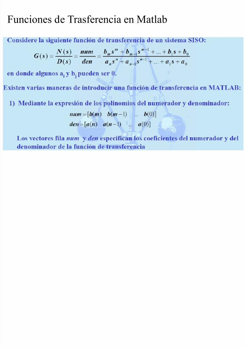
Funciones de Trasferencia en Matlab

8/17/2019 Modelado en Matlab y Simulink
http://slidepdf.com/reader/full/modelado-en-matlab-y-simulink 3/25
Funciones de Trasferencia enMatlab

8/17/2019 Modelado en Matlab y Simulink
http://slidepdf.com/reader/full/modelado-en-matlab-y-simulink 4/25
Ejemplos
Escribir en Matlab las siguientes funciones de
trasferencia:

8/17/2019 Modelado en Matlab y Simulink
http://slidepdf.com/reader/full/modelado-en-matlab-y-simulink 5/25
Conversin de una funcin de trasferencia a
formato !anancia"polo"cero y viceversa
8/17/2019 Modelado en Matlab y Simulink
http://slidepdf.com/reader/full/modelado-en-matlab-y-simulink 6/25
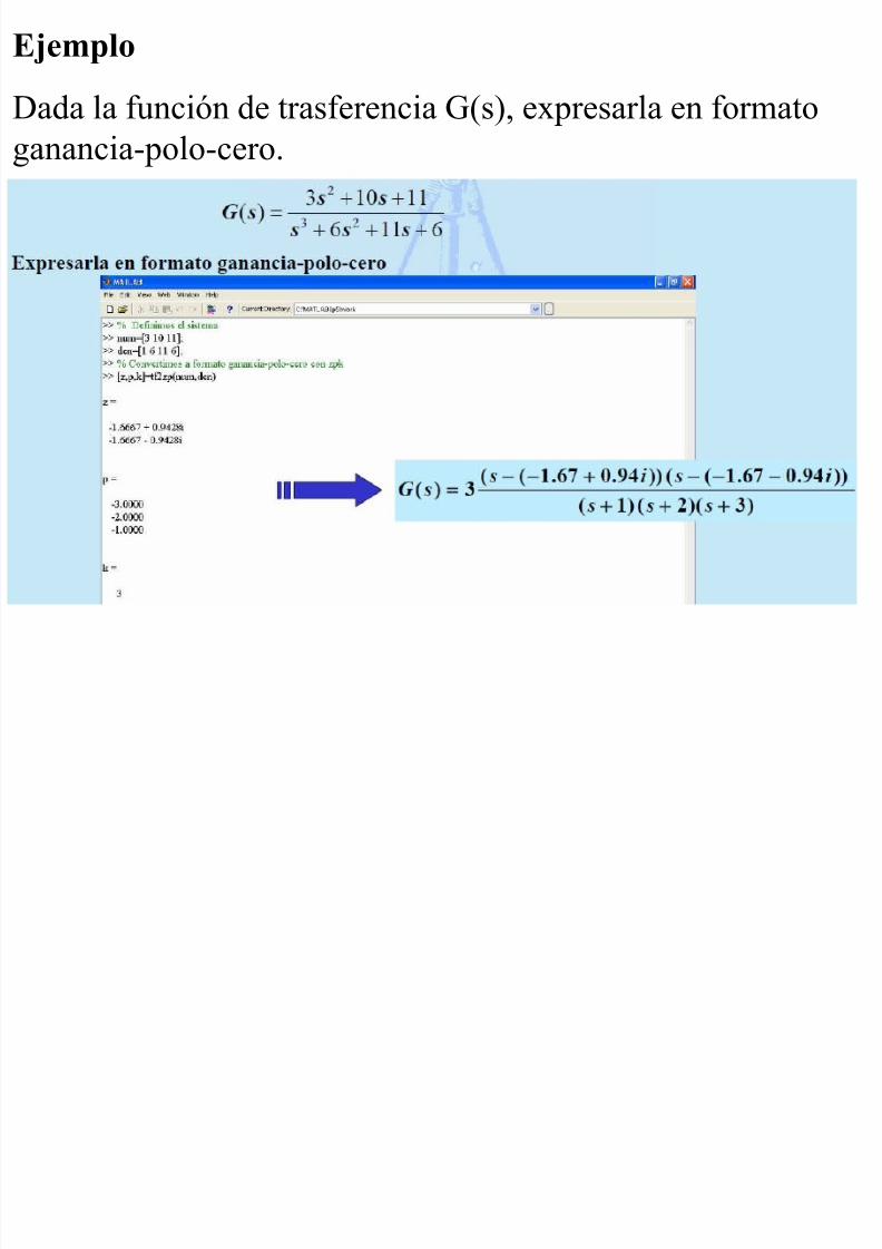
Ejemplo
#ada la funcin de trasferencia $%s&' e(presarla en formato
!anancia"polo"cero)
8/17/2019 Modelado en Matlab y Simulink
http://slidepdf.com/reader/full/modelado-en-matlab-y-simulink 7/25
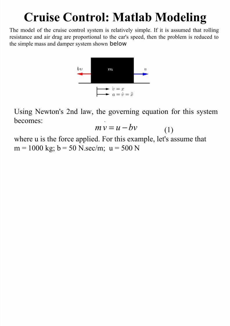
Cruise Control: Matlab Modeling
*sin! +e,ton-s .nd la,' the !overnin! e/uation for this system
becomes0 %1&
,here u is the force applied) For this e(ample' let-s assume that
m 2 1333 k!4 b 2 53 +)sec6m4 u 2 533 +
The model of the cruise control system is relatively simple) 7f it is assumed that rollin!
resistance and air dra! are proportional to the car-s speed' then the problem is reduced to
the simple mass and damper system sho,n below
bvuvm −=)
8/17/2019 Modelado en Matlab y Simulink
http://slidepdf.com/reader/full/modelado-en-matlab-y-simulink 8/25
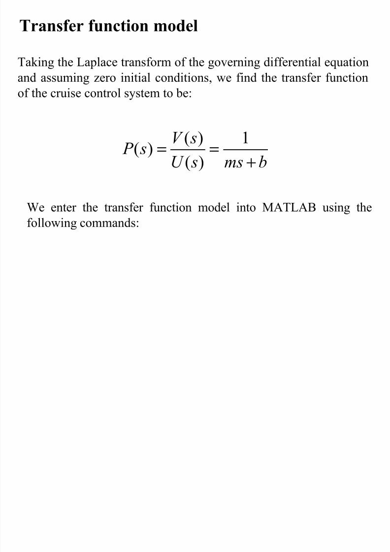
Transfer function model
Takin! the Laplace transform of the !overnin! differential e/uationand assumin! zero initial conditions' ,e find the transfer function
of the cruise control system to be0
bms sU
sV s P +
== 1&%&%&%
8e enter the transfer function model into M9TL9: usin! thefollo,in! commands0
8/17/2019 Modelado en Matlab y Simulink
http://slidepdf.com/reader/full/modelado-en-matlab-y-simulink 9/25
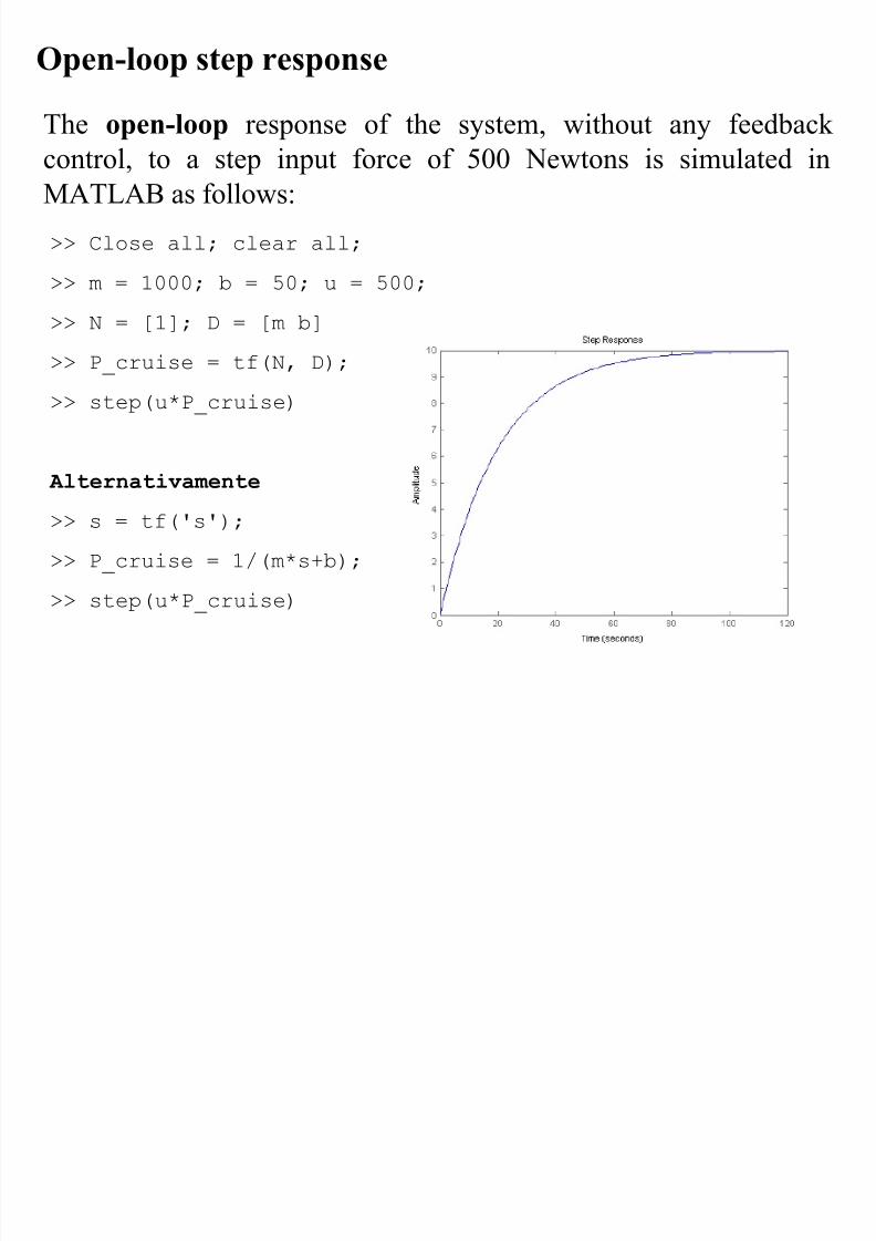
Open-loop step response
The open-loop response of the system' ,ithout any feedback
control' to a step input force of 533 +e,tons is simulated inM9TL9: as follo,s0
>> Close all; clear all;
>> m = 1000; b = 50; u = 500;
>> N = [1]; D = [m b]
>> P_cruise = tf(N, D);
>> step(uP_cruise)
Alternativamente
>> s = tf(!s!);
>> P_cruise = 1"(ms#b);
>> step(uP_cruise)

8/17/2019 Modelado en Matlab y Simulink
http://slidepdf.com/reader/full/modelado-en-matlab-y-simulink 10/25
Building the model in simulink
This system ,ill be modeled by summin! the forces actin! on the mass and inte!ratin! the
acceleration to !ive the velocity) ;pen Simulink and open a ne, model ,indo,) First' ,e ,ill
model the inte!ral of acceleration)
∫ = vdt dt
dv
<7nsert an 7nte!rator :lock %from the Continuous library& and dra, lines to and from its input
and output terminals)<Label the input line =vdot= and the output line =v= as sho,n belo,) To add such a label'
double click in the empty space just above the line)

8/17/2019 Modelado en Matlab y Simulink
http://slidepdf.com/reader/full/modelado-en-matlab-y-simulink 11/25
Since the acceleration %dv6dt& is e/ual to the sum of the forces divided by mass' ,e
,ill divide the incomin! si!nal by the mass)<7nsert a $ain block %from the Math ;perations library& connected to the 7nte!rator
block input line and dra, a line leadin! to the input of the $ain block)
<Edit the $ain block by double"clickin! on it and chan!e its value to =16m=)<Chan!e the label of the $ain block to =inertia= by clickin! on the ,ord =$ain=
underneath the block)
8/17/2019 Modelado en Matlab y Simulink
http://slidepdf.com/reader/full/modelado-en-matlab-y-simulink 12/25
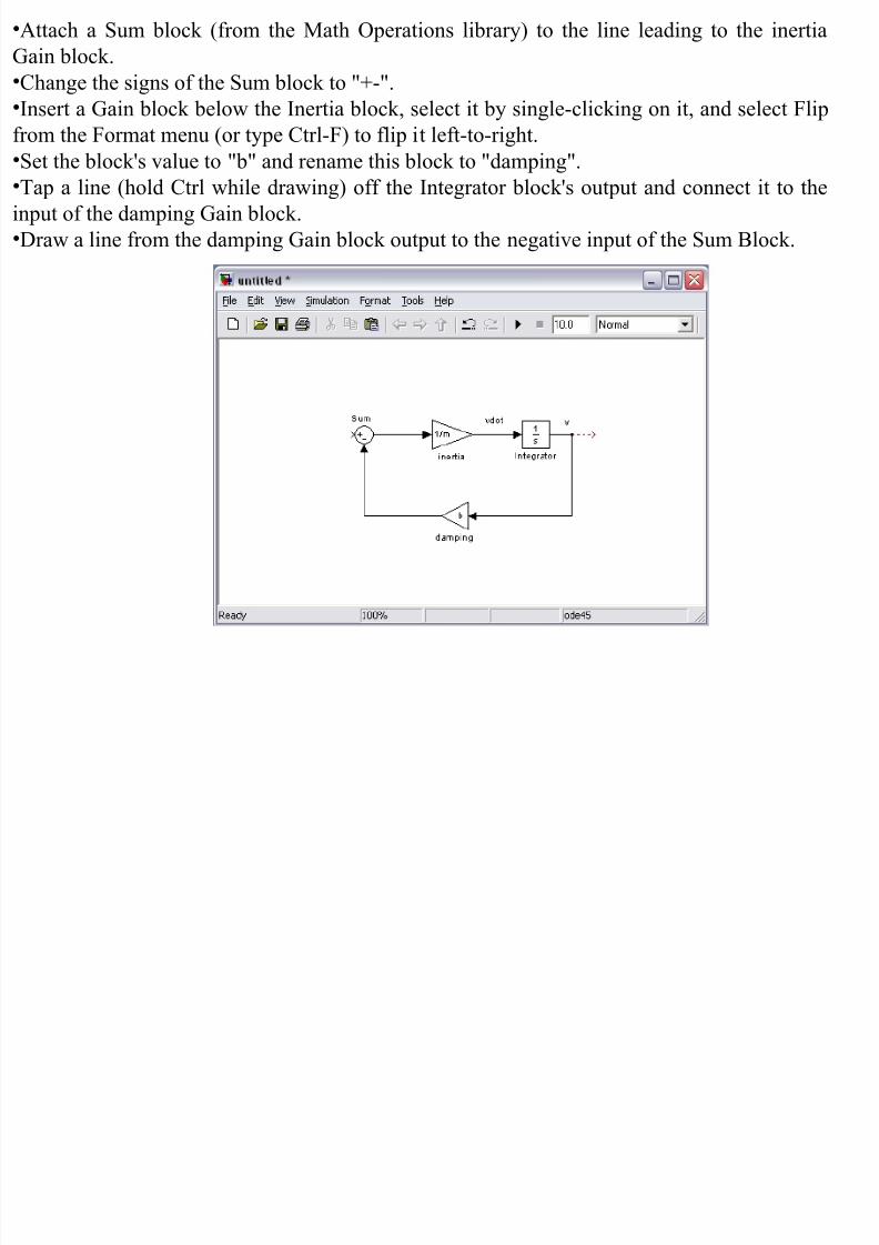
<9ttach a Sum block %from the Math ;perations library& to the line leadin! to the inertia
$ain block)
<Chan!e the si!ns of the Sum block to =>"=)<7nsert a $ain block belo, the 7nertia block' select it by sin!le"clickin! on it' and select Flip
from the Format menu %or type Ctrl"F& to flip it left"to"ri!ht)
<Set the block-s value to =b= and rename this block to =dampin!=)<Tap a line %hold Ctrl ,hile dra,in!& off the 7nte!rator block-s output and connect it to the
input of the dampin! $ain block)
<#ra, a line from the dampin! $ain block output to the ne!ative input of the Sum :lock)

8/17/2019 Modelado en Matlab y Simulink
http://slidepdf.com/reader/full/modelado-en-matlab-y-simulink 13/25
The second force acting on the mass is the control input, u. We will apply astep input.•Insert a tep bloc! "from the ources library# and connect it with a line tothe positi$e input of the um %loc!.• To $iew the output $elocity, insert a cope bloc! "from the in!s library#connected to the output of the Integrator.
8/17/2019 Modelado en Matlab y Simulink
http://slidepdf.com/reader/full/modelado-en-matlab-y-simulink 14/25
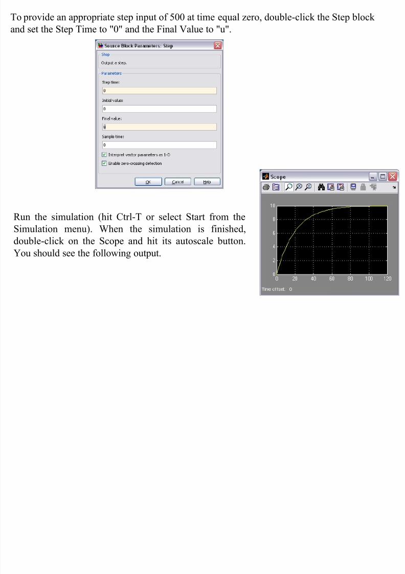
To provide an appropriate step input of 533 at time e/ual zero' double"click the Step block
and set the Step Time to =3= and the Final ?alue to =u=)
@un the simulation %hit Ctrl"T or select Start from the
Simulation menu&) 8hen the simulation is finished'
double"click on the Scope and hit its autoscale button)
Aou should see the follo,in! output)

8/17/2019 Modelado en Matlab y Simulink
http://slidepdf.com/reader/full/modelado-en-matlab-y-simulink 15/25
Modelado en Simulink de . blo/ues
acoplados
#eterminar las E#;s para los . blo/ues %5 Min&
The system that is bein!
analyzed is sho, in the
follo,in! dia!ram
7n the above' is to be taken as each of the follo,in!1) *nit impulse force)
.) *nit step force)
B) Sin%,t&
7t is re/uired to nd (1 y (. usin! Matlab-s Simulink soft,are for the analysis)

8/17/2019 Modelado en Matlab y Simulink
http://slidepdf.com/reader/full/modelado-en-matlab-y-simulink 16/25
Modelado en Simulink de .blo/ue
acoplados

8/17/2019 Modelado en Matlab y Simulink
http://slidepdf.com/reader/full/modelado-en-matlab-y-simulink 17/25
Modelado en Simulink

8/17/2019 Modelado en Matlab y Simulink
http://slidepdf.com/reader/full/modelado-en-matlab-y-simulink 18/25
DC Motor Speed: Simulink Modeling
9 common actuator in control systems is the #C motor) 7t directly provides rotary motion
and' coupled ,ith ,heels or drums and cables' can provide translational motion) The
electric circuit of the armature and the free"body dia!ram of the rotor are sho,n in the
follo,in! fi!ure0
For this e(ample' ,e ,ill assume that the input of the system is the volta!e source %V &
applied to the motor-s armature' ,hile the output is the rotational speed of the shaft
d%theta&6dt) The rotor and shaft are assumed to be ri!id) 8e further assume a viscous
friction model' that is' the friction tor/ue is proportional to shaft an!ular velocity)

8/17/2019 Modelado en Matlab y Simulink
http://slidepdf.com/reader/full/modelado-en-matlab-y-simulink 19/25
Darámetros fsicos para nuestro ejemplo son0
%& Moment of inertia of the rotor 3)31 k!)mG.
%b& Motor viscous friction constant 3)1 +)m)s
% K e& Electromotive force constant 3)31 ?6rad6sec
% K t& Motor tor/ue constant 3)31 +)m69mp
%@& Electric resistance 1 ;hm
%L& Electric inductance 3)5 H
i K T t =
)
θ e
K e =
Tor/ue %T &0
La fuerza electromotriz de
retroceso %e&0

8/17/2019 Modelado en Matlab y Simulink
http://slidepdf.com/reader/full/modelado-en-matlab-y-simulink 20/25
unci!n de trasferencia
Las ecuaciones diferenciales /ue !obiernan el sistema son0
dt
d KeV eV Ri
dt
di L
i K T dt d b
dt d J
t
θ
θ θ
−+=−+=+
==+.
.
9pplyin! the Laplace transform' the above modelin! e/uations can be e(pressed in terms of the Laplace variable s)
&%&%&%&%
&%&%&%
s K sV s I R LS
s I K sb Js s
e
t
θ
θ
−=+
=+
The open&loop transfer function by eliminating I"s# between the twoabo$e e'uations, where the rotational speed is considered the outputand the armature $oltage is considered the input, is:.
et
t
K K b Js R Ls
K
sV
s
−++=
&%I&%&%
&%)
θ

8/17/2019 Modelado en Matlab y Simulink
http://slidepdf.com/reader/full/modelado-en-matlab-y-simulink 21/25
Constru"endo el modelo con Simulink
This system ,ill be modeled by summin! the tor/ues actin! on the
rotor inertia and inte!ratin! the acceleration to !ive velocity) 9lso'
Jirchoff-s la,s ,ill be applied to the armature circuit) First' ,e ,ill
model the inte!rals of the rotational acceleration and of the rate of
chan!e of the armature current)
dt
d dt
dt
d θ θ =∫ .
.
idt
dt
di=∫
&%1
&%1.
.
.
.
dt
d KeV Ri
Ldt
dieV Ri
dt
di L
dt
d bi K
dt
d J
dt
d bT
dt
d J
t
θ
θ θ θ θ
−+−=⇒−+−=
−=⇒−=

8/17/2019 Modelado en Matlab y Simulink
http://slidepdf.com/reader/full/modelado-en-matlab-y-simulink 22/25
To build the simulation model' open Simulink and open a
ne, model ,indo,)

8/17/2019 Modelado en Matlab y Simulink
http://slidepdf.com/reader/full/modelado-en-matlab-y-simulink 23/25

8/17/2019 Modelado en Matlab y Simulink
http://slidepdf.com/reader/full/modelado-en-matlab-y-simulink 24/25

8/17/2019 Modelado en Matlab y Simulink
http://slidepdf.com/reader/full/modelado-en-matlab-y-simulink 25/25