money in the equilibrium of banking · [email protected] abstract in most banking models, money is...

Money in the equilibrium of banking NORGES BANKRESEARCH

22 | 2015

AUTHORS: JIN CAO AND GERHARD ILLING

WORKING PAPER

NORGES BANK

WORKING PAPERXX | 2014

RAPPORTNAVN

2

Working papers fra Norges Bank, fra 1992/1 til 2009/2 kan bestilles over e-post: [email protected]

Fra 1999 og senere er publikasjonene tilgjengelige på www.norges-bank.no Working papers inneholder forskningsarbeider og utredninger som vanligvis ikke har fått sin endelige form. Hensikten er blant annet at forfatteren kan motta kommentarer fra kolleger og andre interesserte. Synspunkter og konklusjoner i arbeidene står for forfatternes regning.

Working papers from Norges Bank, from 1992/1 to 2009/2 can be ordered by e-mail:[email protected]

Working papers from 1999 onwards are available on www.norges-bank.no

Norges Bank’s working papers present research projects and reports (not usually in their final form) and are intended inter alia to enable the author to benefit from the comments of colleagues and other interested parties. Views and conclusions expressed in working papers are the responsibility of the authors alone.

ISSN 1502-819-0 (online) ISBN 978-82-7553-889-3 (online)

1

Money in the Equilibrium of Banking1

Jin Cao

Research Department, Norges Bank, Bankplassen 2, P. O. Box 1179 Sentrum, N-0107 Oslo, Norway

and CESifo, Germany

[email protected]

Gerhard Illing

Seminar für Makroökonomie, Ludwig-Maximilians-Universität München, Ludwigstrasse 28/012

(Rgb.), D-80539 Munich, Germany and CESifo, Germany

[email protected]

Abstract

In most banking models, money is merely modeled as a medium of transactions, but in reality, money

is also the most liquid asset for banks. Central banks do not only passively supply money to meet

demand for transactions, as often assumed in these models, instead they also actively inject liquidity

into market, taking banks’ illiquid assets as collateral. We examine both roles of money in an

integrated framework, in which banks are subject to aggregate illiquidity risk. With fixed nominal

deposit contracts, the monetary economy with an active central bank can replicate constrained efficient

allocation. This allocation, however, cannot be implemented in market equilibrium without additional

regulation: Due to moral hazard problems, banks invest excessively in illiquid assets, forcing the

central bank to provide liquidity at low interest rates. We show that interest rate policy to reduce

systemic liquidity risk on its own is dynamically inconsistent. Instead, the constrained efficient

solution can be achieved by imposing an ex ante liquidity coverage requirement.

Keywords: Central banking; liquidity facility; systemic liquidity risk

JEL classification: G21; G28

1 Introduction

After the financial crisis in 2008, concerns about financial stability and the disruption of financial

intermediation have become a key focus for central banks. Unconventional monetary policy measures

such as credit easing try to prevent systemic banking crises. At the same time, there are increasing

concerns that accommodative monetary policy with ample liquidity provision may encourage

excessive risk taking, resulting in a rapid increase in the leverage of financial intermediation and so

endangering financial stability in the future. Our paper tries to analyze the feedback mechanism

between central bank actions and banks’ incentives to cope with liquidity risk in a fiat money

economy.

Traditional banking models are real models without fiat money. Even though they provide useful

insights on the sources of financial instability, they are silent on the question of what impact liquidity

1 This working paper should not be reported as representing the views of Norges Bank. The views expressed are

those of the authors and do not necessarily reflect those of Norges Bank. The authors thank Farooq Akram,

Valeriya Dinger, Artashes Karapetyan and participants in various seminars for very helpful comments.

2

provision via fiat money has on financial stability in reality. Recently, several studies, such as Allen et

al. (2014) and Skeie (2008), try to fill this gap. In these models, money is mostly used only as the

medium for transactions. The central bank merely issues bank notes passively to meet the money

demand for transactions (in Allen et al., 2014 even the banks are passive: they pass deposits to firms

which make decisions on investment portfolios). As a result, the (constrained) efficient equilibrium

can always be achieved as long as depositors’ nominal claims are met: In these models, monetary

economy either replicates the first best allocation in the real economy – since money is only used as

the medium for transaction, or improves social welfare by eliminating costly bank runs – as long as the

central bank issues sufficient fiat money so that all the banks can meet their nominal deposit contracts.

However, in reality fiat money is not only the medium for transactions, but also the most liquid asset

in the banking sector. Central banks take a much more active role by providing liquidity to the

economy. Traditionally, the quantity theory of money focuses on the role of money as medium of

transactions, with the price level being determined by the aggregate supply of money. The New

Keynesian (“Woodfordian”) monetary theory focuses on interest rate adjustments as mechanism for

stabilizing the price level. However, in both perspectives banks essentially do nothing more than

passively transmitting money into the real economy. The contribution of this paper is to capture both

perspectives in one framework, analyzing the impact of banks’ strategies on money demand, inflation,

and financial stability in a purely monetary economy.

Apart from monetizing transactions, central banks also conduct active monetary policy, using short-

term interest rates to affect banks’ refinancing cost in the market for liquidity. Here, banks use their

illiquid assets – which provide return in the future – as collateral to raise money as liquid asset in order

to meet depositors’ demand for liquidity today. Now the role of central bank has been significantly

changed in our model: It is no longer a passive provider of fiat money, but an active player of maturity

transformation in banking. Money as liquidity and the central bank’s monetary policy practice have

profound implications for financial stability: Banks can now react actively to the path of the central

bank’s policy rate, exploiting the central bank’s liquidity facilities to reshuffle resources across

periods, whenever possible, by increasing the share of high-yield illiquid assets in their investment

portfolios. Such strategic feedback between the central bank’s monetary policy and banks’ investment

decisions, as this paper shows, may become a source of systemic risk such that banks are engaged in

excessive liquidity risks and the economy gets stuck in an inferior equilibrium.

In this paper, we start with a baseline model of a real economy, where banks are involved in maturity

transformation: Impatient depositors get paid by return from banks’ short (liquid) assets, and banks

can roll over their debts by borrowing from the liquidity market, using their long (illiquid) assets as

collateral. Banks therefore have an incentive to hold liquid assets to meet depositors’ demand for

idiosyncratic risks, while negative aggregate liquidity shocks lead to aggregate liquidity shortages and

trigger system-wide bank runs, generating huge social costs. Using the same setup, we show that in a

decentralized monetary economy with the central bank providing money both as medium of

transaction as well as bank liquidity, banks can get access to liquidity through the central bank’s

interday loans, using their long maturity assets as collateral. Costly bank runs will be then eliminated

and the constrained efficient allocation can be replicated. However, this allocation cannot be

implemented as dynamic consistent equilibrium due to the moral hazard arising from the central

bank’s commitment to provide standing liquidity facilities: Banks will always have the incentive to

invest excessively in illiquid assets, leaving the depositors too low real return; the constrained efficient

equilibrium breaks down, and the monetary economy ends up in an inferior equilibrium. To restore

constrained efficiency, we argue that the central bank’s liquidity facility should not be conditioned on

3

the banks’ liquidity due to the time-inconsistency problem; instead, liquidity support should be made

contingent on the banks’ fulfilling liquidity constraints as entry requirement.

1.1 Related literature

Freixas, Martin and Skeie (2011) analyze the efficiency of the interbank lending market in allocating

funds and the optimal policy of a central bank in response to liquidity shocks. They show that, during

an aggregate liquidity crisis, central banks need to manage both interest rates and liquidity injection

(the aggregate volume of liquidity). In their model, failure to cut interest rates during a crisis erodes

financial stability by increasing the probability of bank runs. They do not, however, address the

feedback mechanism between the central bank’s policy and the incentives of the banking system to

invest in private provision of liquid assets.

Allen, Carletti and Gale (2014) introduce nominal contracts in a banking model with idiosyncratic and

aggregate liquidity risk. They show that the first-best efficient allocation can be achieved in a

decentralized banking system when the central bank accommodates the demands of the private sector

for fiat money. In their model, variations in the price level allow full sharing of aggregate risks. Their

paper, however, does not analyze how financial intermediaries react ex ante to anticipated liquidity

injections by the central bank. The probability of an aggregate liquidity shock is not affected by the

amount of private investment in liquid assets. In contrast, our paper focuses explicitly on the

endogenous response of private banks to liquidity injections. We show that they engage in activities

creating systemic risk by investing in less liquid assets.

Our paper extends Cao and Illing (2011). That paper characterizes incentives for private liquidity

provision in a static framework when the central bank mitigates the fragility of the financial system

arising from banks liquidity transformation via nominal deposit contracts. Here, we analyze a repeated

setting of Cao and Illing (2011), focusing on the case where systemic shocks are extremely rare

events. In case of a systemic shock, the central bank, trying to prevent costly bank runs, provides

additional paper money to the banks. Lender of last resort policy prevents interest rates from shooting

up in case of systemic risk, ensuring that banks are always able to pay out their nominal commitments.

We show that the central bank may be forced to keep interest rates low for an extended period,

crowding out private liquidity provision.

1.2 Structure of the paper

Section 2 presents the structure of the model in a real economy and characterizes the constrained

efficient solution. Section 3 shows that in a decentralized monetary economy with the central bank

providing money both as medium of transaction as well as bank liquidity, costly bank runs can be

eliminated and the constrained efficient allocation can be replicated. However, section 4 shows that

this allocation cannot be implemented as dynamic consistent equilibrium due to the moral hazard

arising from the central bank’s commitment to provide standing liquidity facilities, and section 5

further shows that the same result holds in the long-run equilibrium. Section 6 proposes liquidity

requirement as solution to restore efficiency in the monetary economy. Section 7 concludes.

2 The real economy

4

In this section we consider the real economy. Following Cao and Illing (2011), we describe the source

of liquidity risk and, as the baseline result for the rest of the paper, characterize the constrained

efficient allocation.

2.1 The model setup

Consider the following economy with three types of risk-neutral agents: depositors, banks (run by

bank managers), and entrepreneurs. The economy extends over three periods, 𝑡 = 0, 1, 2, and the

details of timing will be explained later. We assume that:

(i) There is a continuum of depositors, each being endowed with one unit of resources at 𝑡 = 0. They

will be willing to deposit in banks as long as the real return is (weakly) larger than 1. Depositors are

impatient: they want to withdraw and consume at 𝑡 = 1; in contrast, banks and entrepreneurs are

indifferent between consuming at 𝑡 = 1 and 𝑡 = 2;

(ii) There is a finite number 𝑁 of active banks participating in Bertrand competition, competing for

depositors’ deposits at 𝑡 = 0. Using these deposits, banks as financial intermediaries can fund the

projects of entrepreneurs;

(iii) There is a continuum of entrepreneurs, and there are sufficiently many entrepreneurs competing

for funds so that bank deposits are scarce. Each of the entrepreneurs runs one of two types of projects:

• Safe projects, which are realized early at 𝑡 = 1 with a safe return 𝑅1 > 1.

• Risky projects, which give a higher return 𝑅2 > 𝑅1 > 1. With probability 𝑝, these projects will be

realized at 𝑡 = 1, but the return may be delayed (with probability 1 − 𝑝) until 𝑡 = 2. Therefore, in

the aggregate, the share 𝑝 of type 2 projects will be realized early. The value of 𝑝, however, is not

known at 𝑡 = 0. It will only be revealed between period 0 and 1 at some intermediate period, 𝑡 = 1

2.

In the following, we are interested in the case of aggregate shocks to all risky projects (but we will

discuss idiosyncratic shocks later): The value of 𝑝 can be either 𝑝𝐻 or 𝑝𝐿 with 𝑝𝐻 > 𝑝𝐿. The “good”

state with 𝑝 = 𝑝𝐻will be realized with probability 𝜋. Since the “bad” state, or the “crisis” state, is rare,

we assume that 𝜋 is almost 12. In the following, we further assume that 1 < 𝑝𝑠𝑅2 < 𝑅1 (𝑠 ∈ {𝐻, 𝐿})

to focus on the relevant case.3

At 𝑡 = 0 banks compete for depositors by offering them fixed deposit contracts that promise a return

𝑑0 at 𝑡 = 1. At the same time, banks decide the proportion 𝛼 of deposits to be invested in the safe

assets. Depositors have rational expectations: they deposit in banks that offer them the highest

expected return.

At 𝑡 =1

2 the value of 𝑝 is revealed, and this is public information. Given the value of 𝑝, if one bank

will not be able to meet its depositors’ claims at 𝑡 = 1, the depositors will run on the bank at 𝑡 =1

2

because of first-come-first-served rule. If a bank experiences a run at this date, it has to liquidate all

2 As long as 𝜋 ∈ (

𝛾𝐸[𝑅𝐿]−𝑐

𝛾𝐸[𝑅𝐻]−𝑐, 1) with 𝐸[𝑅𝑠] = 𝛼𝑠𝑅1 + (1 − 𝛼𝑠)𝑅2 (𝑠 ∈ {𝐿, 𝐻}) and 𝛼𝑠 =

𝛾−𝑝𝑠

𝛾−𝑝𝑠+(1−𝛾)𝑅1𝑅2

. This

allows us to focus on the case that the cost of bank failure is small enough that banks can take more

liquidity risk instead of investing higher share on liquid assets to avoid bank runs completely. 3 In that case, depositors care about the share invested in liquid projects. On the other hand, due to

financial frictions captured by the hold-up problem as characterized at the end of this section,

depositors gain from banks also investing some share in illiquid projects.

5

unmatured assets, i.e., both safe and risky projects. Each unit of liquidated asset yields a poor return

𝑐 < 1.

If there is no bank run, banks collect a proportion 𝛾 from the return of early projects (safe projects plus

those risky projects that return early) and early entrepreneurs retain the rest (the implication of 𝛾 will

be explained later). To maximize depositors’ return, banks can raise more funds from early

entrepreneurs in the liquidity market: banks borrow from early entrepreneurs, promising a borrowing

rate 𝑟 and using their late projects as collateral. Since entrepreneurs are indifferent between consuming

at 𝑡 = 1 and 𝑡 = 2, they will be willing to lend to banks as long as 𝑟 ≥ 1. Banks make payouts to

depositors using the return collected from early projects and the liquidity borrowed from the liquidity

market.

At 𝑡 = 2 banks collect return from late projects and pay back early entrepreneurs.

If there were no financial friction, depositors would contract directly with entrepreneurs, investing

entirely in the safe projects, and receive all the return at 𝑡 = 1. However, due to hold-up problems as

modeled in Hart and Moore (1994), entrepreneurs can only commit to pay a fraction 𝛾 of their return

(assume that 𝛾𝑅𝑖 > 1). Banks as financial intermediaries are assumed to have better collection skills

(higher 𝛾) than depositors, so that depositors become better off by depositing their endowments in

banks. However, as is shown in Diamond and Rajan (2001), banks then have the incentive to abuse

their collection skills and force depositors to renegotiate at 𝑡 = 1, resulting in a breakdown of deposit

contracts. To avoid this, banks need to offer fixed deposit contracts, as is assumed in this paper, and

depositors are entitled to run once they perceive that banks cannot meet the contracts, leaving all

banks’ assets destroyed. The threat of bank run is thus a device to discipline banks to respect deposit

contracts.

2.2 The constrained efficient allocation

The baseline of the model is the constrained efficient allocation, achieved from the solution of the

social planner’s problem. This will be the reference point for the market equilibrium characterized in

the next section, when banks serve as financial intermediaries. Assume that the social planner has the

same collection skill (the same 𝛾) as banks, and she maximizes the depositors’ real return by choosing

a portfolio of safe and risky assets. The result is characterized in the following proposition:

Proposition 1 The constrained efficient allocation is featured by

(1) At 𝑡 = 0 the planner invests a share 𝛼𝐻 =𝛾−𝑝𝐻

𝛾−𝑝𝐻+(1−𝛾)𝑅1𝑅2

on the safe assets, and the depositors’

expected return at 𝑡 = 1 is 𝐸[𝑅(𝛼𝐻)] = 𝜋𝛾𝐸[𝑅𝐻] + (1 − 𝜋)𝛾𝐸[𝑅𝐿];

(2) When 𝑝𝐿 is realized at 𝑡 =1

2, depositors’ return at 𝑡 = 1 is 𝛼𝐻𝑅1 + (1 − 𝛼𝐻)𝑝𝐿𝑅2 <

𝛾[𝛼𝐻𝑅1 + (1 − 𝛼𝐻)𝑅2].

Proof See Appendix.

Since the social planner cannot reshuffle resources between periods, and depositors only value

consumption at 𝑡 = 1, a share of the funds should be invested in safe projects. However, depositors

will also benefit from social planner’s holding of risky assets, since social planner can raise additional

liquidity from early entrepreneurs and maximize depositors’ return, using the delayed risky projects as

collateral. Given that the likelihood of a bad state is low, the social planner should choose the

investment portfolio such that it maximizes depositors’ return in the good state; while in the bad state,

6

the abundant delayed projects allow social planner to use all the funds held by the early entrepreneurs

at 𝑡 = 1 and return to depositors, even though depositors’ return is lower than that in the good state.

2.3 Market equilibrium

In this section we consider a decentralized economy and characterize market equilibrium with banks.

The equilibrium consists of banks’ strategic profiles (𝛼𝑖∗, 𝑑0𝑖

∗ ), ∀𝑖 ∈ {1, … , 𝑁}, that satisfy the

following conditions:

Profit maximization of banks At 𝑡 = 0 every bank chooses its optimal proportion of investment in

liquid assets 𝛼𝑖∗ and deposit contract 𝑑0𝑖

∗ to maximize its expected return. That is, the bank makes

lower profit if it chooses any different strategic profile

Π𝑖(𝛼𝑖, 𝑑0𝑖) < Π𝑖(𝛼𝑖∗, 𝑑0𝑖

∗ ), ∀(𝛼𝑖, 𝑑0𝑖) ≠ (𝛼𝑖∗, 𝑑0𝑖

∗ );

Zero profit No bank makes positive profit, as a result of Bertrand competition;

Return maximization of depositors At 𝑡 = 0 depositors deposit their endowments at those banks

offering the highest expected return;

Market clearing At 𝑡 = 1, if there is no bank run, the liquidity market is cleared by the interest rate 𝑟

which is offered to the early entrepreneurs by banks.

Since the bad state is a low probability event, banks can take more liquidity risk to maximize their

return in the good state, ignoring the liquidation cost in the bad state. Banks’ return is maximized

when they can obtain the most liquidity at the lowest interest rate. Under the market clearing

condition, the equilibrium interest rate is determined by the value of banks’ late projects and the

volume of liquidity (the rent retained by early entrepreneurs) – both are functions of 𝛼. In the end,

banks’ decision problem boils down to choosing the optimal 𝛼 so that banks can borrow in the

liquidity market at the lowest cost. The equilibrium can be characterized by the following proposition:

Proposition 2 Market equilibrium in the decentralized real economy is featured by

(1) At 𝑡 = 0 all banks set 𝛼∗ = 𝛼𝐻 and offer 𝑑0∗ = 𝛾𝐸[𝑅𝐻];

(2) When 𝑝𝐻 is revealed, banks raise liquidity from the liquidity market at 𝑡 = 1 at interest rate

𝑟 = 1 and repay depositors; when 𝑝𝐿 is revealed, banks experience runs and have to liquidate

both safe and risky projects at 𝑡 =1

2;

(3) Depositors’ expected return is 𝜋𝛾𝐸[𝑅𝐻] + (1 − 𝜋)𝑐, which is inferior to that in the

constrained efficient allocation.

Proof See Appendix.

Compared with the constrained efficient solution as characterized in the previous section, it is evident

that in the decentralized economy banks do have the incentive to hold the same share of liquid assets

in their investment portfolio, which maximizes depositors’ return in the good state. However, when

the bad state is revealed at 𝑡 =1

2 and there is an aggregate liquidity shortage in the economy, banks

cannot raise sufficient funding in the liquidity market. Although banks hold enough delayed projects

which may serve as good collateral, depositors will run the bank, resulting in socially costly

liquidation of all assets. In the next section, we show that costly bank run can be eliminated in a

7

monetary economy, where there is a central bank providing money both as medium of transaction and

bank liquidity, so the constrained efficient solution can be replicated.

3 Constrained efficiency in a decentralized monetary economy

In this section, we show that the constrained efficient allocation can be replicated in a decentralized

monetary economy, improving efficiency compared with that under market equilibrium.

From now on, following the model outlined in the previous section, assume there is a central bank

acting as monetary authority, with all deposit contracts being written in nominal terms. We distinguish

two roles of money:

(1) Money as medium of transaction. In our monetary economy, all the transactions are

committed via exchanges of cash versus goods. Fiat money is issued by the central bank to

facilitate the transactions (“monetizing the economy”), and the quantity of money in

circulation is equal to the transaction demand for money. For simplicity, we assume that the

quantity of money issued in each period is equal to the quantity of real goods in transaction,

thus normalizing the price level in the absence of additional liquidity provision to 1.

(2) Money as liquidity. Banks can borrow additional fiat money from the central bank to meet

their demand for liquidity subject to the central bank’s policy rate, using their illiquid assets as

collateral.

Motivated by these two roles of money, monetary policy of the central bank is conducted through the

following two kinds of operations:

(1) Money as medium of transaction is issued through intraday loans to banks during the period.

Its quantity is equal to the quantity of real goods in transaction, and banks have to pay back

the loans in the end of the period. This is the working mechanism of Allen, Carletti and Gale

(2014);

(2) On the other hand, central bank is also a crucial liquidity provider to the banking sector:

Money as liquidity is injected into the economy through interday loans to banks subject to the

policy rate, using banks’ long assets as collateral. The loans are paid back one period later,

after the return of long assets materializes.

8

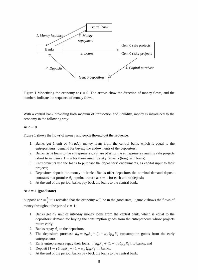
Figure 1 Monetizing the economy at 𝑡 = 0. The arrows show the direction of money flows, and the

numbers indicate the sequence of money flows.

With a central bank providing both medium of transaction and liquidity, money is introduced to the

economy in the following way:

At 𝒕 = 𝟎

Figure 1 shows the flows of money and goods throughout the sequence:

1. Banks get 1 unit of intraday money loans from the central bank, which is equal to the

entrepreneurs’ demand for buying the endowments of the depositors;

2. Banks issue loans to the entrepreneurs, a share of 𝛼 for the entrepreneurs running safe projects

(short term loans), 1 − 𝛼 for those running risky projects (long term loans);

3. Entrepreneurs use the loans to purchase the depositors’ endowments, as capital input to their

projects;

4. Depositors deposit the money in banks. Banks offer depositors the nominal demand deposit

contracts that promise 𝑑0 nominal return at 𝑡 = 1 for each unit of deposit;

5. At the end of the period, banks pay back the loans to the central bank.

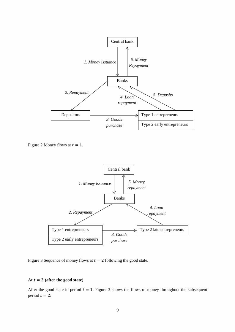
At 𝒕 = 𝟏 (good state)

Suppose at 𝑡 =1

2 it is revealed that the economy will be in the good state, Figure 2 shows the flows of

money throughout the period 𝑡 = 1:

1. Banks get 𝑑0 unit of intraday money loans from the central bank, which is equal to the

depositors’ demand for buying the consumption goods from the entrepreneurs whose projects

return early;

2. Banks repay 𝑑0 to the depositors;

3. The depositors purchase 𝑑0 = 𝛼𝐻𝑅1 + (1 − 𝛼𝐻)𝑝𝐻𝑅2 consumption goods from the early

entrepreneurs;

4. Early entrepreneurs repay their loans, 𝛾[𝛼𝐻𝑅1 + (1 − 𝛼𝐻)𝑝𝐻𝑅2], to banks, and

5. Deposit (1 − 𝛾)[𝛼𝐻𝑅1 + (1 − 𝛼𝐻)𝑝𝐻𝑅2] in banks;


Central bank

Banks Gen. 0 safe projects

Gen. 0 risky projects

Gen. 0 depositors

1. Money issuance

2. Loans

3. Capital purchase 4. Deposits

5. Money

repayment

9

Figure 2 Money flows at 𝑡 = 1.

Figure 3 Sequence of money flows at 𝑡 = 2 following the good state.

At 𝒕 = 𝟐 (after the good state)

After the good state in period 𝑡 = 1, Figure 3 shows the flows of money throughout the subsequent

period 𝑡 = 2:

Central bank

Banks

Type 1 entrepreneurs

Type 2 early entrepreneurs

Depositors

1. Money issuance

2. Repayment 5. Deposits

3. Goods

purchase

4. Loan

repayment

6. Money

Repayment

Banks



Type 2 late entrepreneurs

2. Repayment

3. Goods

purchase

4. Loan

repayment

Central bank

1. Money issuance 5. Money

repayment

10

1. Banks get (1 − 𝛾)[𝛼𝐻𝑅1 + (1 − 𝛼𝐻)𝑝𝐻𝑅2] unit of intraday money loans from the central

bank, which is equal to early entrepreneurs’ demand for buying the consumption goods from

late entrepreneurs;

2. Banks repay (1 − 𝛾)[𝛼𝐻𝑅1 + (1 − 𝛼𝐻)𝑝𝐻𝑅2] to early entrepreneurs;

3. Early entrepreneurs purchase (1 − 𝛾)[𝛼𝐻𝑅1 + (1 − 𝛼𝐻)𝑝𝐻𝑅2] = 𝛾(1 − 𝛼𝐻)(1 − 𝑝𝐻)𝑅2

consumption goods from the late entrepreneurs;

4. Late entrepreneurs repay their loans, 𝛾(1 − 𝛼𝐻)(1 − 𝑝𝐻)𝑅2, to banks;

5. At the end of the period, banks pay back all the loans to the central bank.

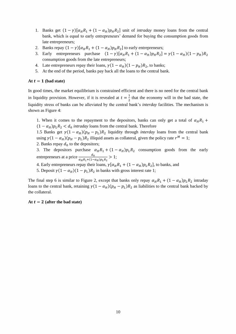
At 𝒕 = 𝟏 (bad state)

In good times, the market equilibrium is constrained efficient and there is no need for the central bank

in liquidity provision. However, if it is revealed at 𝑡 =1

2 that the economy will in the bad state, the

liquidity stress of banks can be alleviated by the central bank’s interday facilities. The mechanism is

shown as Figure 4:

1. When it comes to the repayment to the depositors, banks can only get a total of 𝛼𝐻𝑅1 +

(1 − 𝛼𝐻)𝑝𝐿𝑅2 < 𝑑0 intraday loans from the central bank. Therefore

1.5 Banks get 𝛾(1 − 𝛼𝐻)(𝑝𝐻 − 𝑝𝐿)𝑅2 liquidity through interday loans from the central bank

using 𝛾(1 − 𝛼𝐻)(𝑝𝐻 − 𝑝𝐿)𝑅2 illiquid assets as collateral, given the policy rate 𝑟𝑀 = 1;

2. Banks repay 𝑑0 to the depositors;

3. The depositors purchase 𝛼𝐻𝑅1 + (1 − 𝛼𝐻)𝑝𝐿𝑅2 consumption goods from the early

entrepreneurs at a price 𝑑0

𝛼𝐻𝑅1+(1−𝛼𝐻)𝑝𝐿𝑅2> 1;

4. Early entrepreneurs repay their loans, 𝛾[𝛼𝐻𝑅1 + (1 − 𝛼𝐻)𝑝𝐿𝑅2], to banks, and

5. Deposit 𝛾(1 − 𝛼𝐻)(1 − 𝑝𝐿)𝑅2 in banks with gross interest rate 1;

The final step 6 is similar to Figure 2, except that banks only repay 𝛼𝐻𝑅1 + (1 − 𝛼𝐻)𝑝𝐿𝑅2 intraday

loans to the central bank, retaining 𝛾(1 − 𝛼𝐻)(𝑝𝐻 − 𝑝𝐿)𝑅2 as liabilities to the central bank backed by

the collateral.

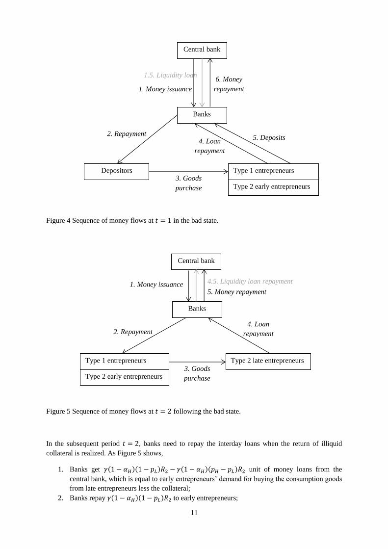
At 𝒕 = 𝟐 (after the bad state)

11

Figure 4 Sequence of money flows at 𝑡 = 1 in the bad state.

Figure 5 Sequence of money flows at 𝑡 = 2 following the bad state.

In the subsequent period 𝑡 = 2, banks need to repay the interday loans when the return of illiquid

collateral is realized. As Figure 5 shows,

1. Banks get 𝛾(1 − 𝛼𝐻)(1 − 𝑝𝐿)𝑅2 − 𝛾(1 − 𝛼𝐻)(𝑝𝐻 − 𝑝𝐿)𝑅2 unit of money loans from the

central bank, which is equal to early entrepreneurs’ demand for buying the consumption goods

from late entrepreneurs less the collateral;

2. Banks repay 𝛾(1 − 𝛼𝐻)(1 − 𝑝𝐿)𝑅2 to early entrepreneurs;

Central bank

Banks



Depositors

1. Money issuance

2. Repayment 5. Deposits

3. Goods

purchase

4. Loan

repayment

6. Money

repayment

1.5. Liquidity loan

Banks



Type 2 late entrepreneurs

2. Repayment

3. Goods

purchase

4. Loan

repayment

Central bank

1. Money issuance 5. Money repayment

4.5. Liquidity loan repayment

12

3. Early entrepreneurs purchase 𝛾(1 − 𝛼𝐻)(1 − 𝑝𝐿)𝑅2 consumption goods from late

entrepreneurs;

4. Late entrepreneurs repay their loans, 𝛾(1 − 𝛼𝐻)(1 − 𝑝𝐿)𝑅2, to banks.

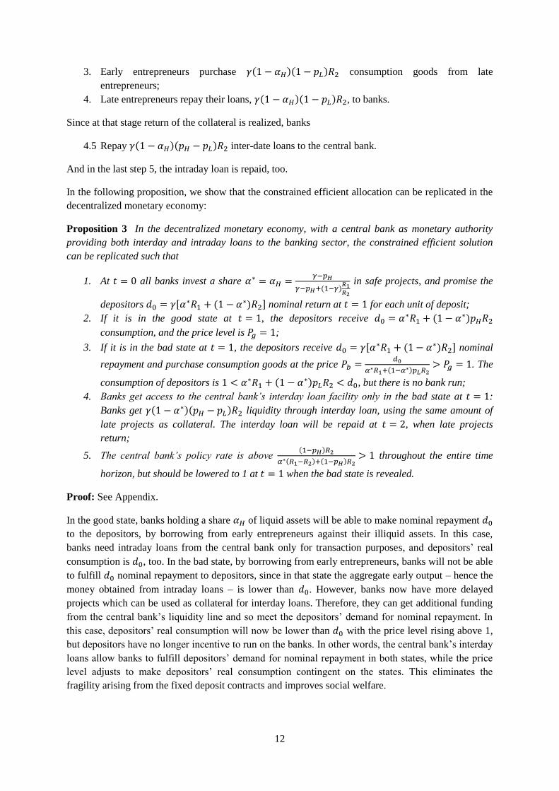
Since at that stage return of the collateral is realized, banks

4.5 Repay 𝛾(1 − 𝛼𝐻)(𝑝𝐻 − 𝑝𝐿)𝑅2 inter-date loans to the central bank.

And in the last step 5, the intraday loan is repaid, too.

In the following proposition, we show that the constrained efficient allocation can be replicated in the

decentralized monetary economy:

Proposition 3 In the decentralized monetary economy, with a central bank as monetary authority

providing both interday and intraday loans to the banking sector, the constrained efficient solution

can be replicated such that

1. At 𝑡 = 0 all banks invest a share 𝛼∗ = 𝛼𝐻 =𝛾−𝑝𝐻


in safe projects, and promise the

depositors 𝑑0 = 𝛾[𝛼∗𝑅1 + (1 − 𝛼∗)𝑅2] nominal return at 𝑡 = 1 for each unit of deposit;

2. If it is in the good state at 𝑡 = 1, the depositors receive 𝑑0 = 𝛼∗𝑅1 + (1 − 𝛼∗)𝑝𝐻𝑅2

consumption, and the price level is 𝑃𝑔 = 1;

3. If it is in the bad state at 𝑡 = 1, the depositors receive 𝑑0 = 𝛾[𝛼∗𝑅1 + (1 − 𝛼∗)𝑅2] nominal

repayment and purchase consumption goods at the price 𝑃𝑏 =𝑑0

𝛼∗𝑅1+(1−𝛼∗)𝑝𝐿𝑅2> 𝑃𝑔 = 1. The

consumption of depositors is 1 < 𝛼∗𝑅1 + (1 − 𝛼∗)𝑝𝐿𝑅2 < 𝑑0, but there is no bank run;

4. Banks get access to the central bank’s interday loan facility only in the bad state at 𝑡 = 1:

Banks get 𝛾(1 − 𝛼∗)(𝑝𝐻 − 𝑝𝐿)𝑅2 liquidity through interday loan, using the same amount of

late projects as collateral. The interday loan will be repaid at 𝑡 = 2, when late projects

return;

5. The central bank’s policy rate is above (1−𝑝𝐻)𝑅2

𝛼∗(𝑅1−𝑅2)+(1−𝑝𝐻)𝑅2> 1 throughout the entire time

horizon, but should be lowered to 1 at 𝑡 = 1 when the bad state is revealed.

Proof: See Appendix.

In the good state, banks holding a share 𝛼𝐻 of liquid assets will be able to make nominal repayment 𝑑0

to the depositors, by borrowing from early entrepreneurs against their illiquid assets. In this case,

banks need intraday loans from the central bank only for transaction purposes, and depositors’ real

consumption is 𝑑0, too. In the bad state, by borrowing from early entrepreneurs, banks will not be able

to fulfill 𝑑0 nominal repayment to depositors, since in that state the aggregate early output – hence the

money obtained from intraday loans – is lower than 𝑑0. However, banks now have more delayed

projects which can be used as collateral for interday loans. Therefore, they can get additional funding

from the central bank’s liquidity line and so meet the depositors’ demand for nominal repayment. In

this case, depositors’ real consumption will now be lower than 𝑑0 with the price level rising above 1,

but depositors have no longer incentive to run on the banks. In other words, the central bank’s interday

loans allow banks to fulfill depositors’ demand for nominal repayment in both states, while the price

level adjusts to make depositors’ real consumption contingent on the states. This eliminates the

fragility arising from the fixed deposit contracts and improves social welfare.

13

4 Market equilibrium in the monetary economy and systemic liquidity risk

The key mechanism to replicate the constraint efficient solution hinges on the central bank’s interest

rate policy, which works through the liquidity facility. The policy rate should be so high in the normal

state that banks are induced to implement the first best equilibrium, while it should be low enough in

the crisis state that banks are guaranteed for sufficient liquidity through the central bank’s liquidity

facility.

However, the central bank’s commitment to a high policy rate in the normal state, which intends to

deter banks’ incentive to over-invest in illiquid assets, is an noncredible threat. Since the social cost of

bank failure is too high, it is ex post optimal for the central bank to bail out the illiquid banks even in

the normal state. Such a time-inconsistency problem is characterized by the following proposition:

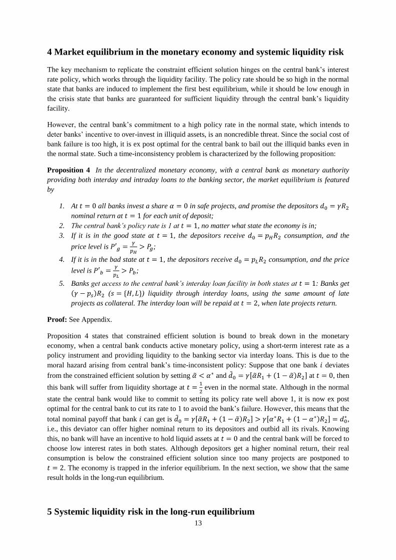
Proposition 4 In the decentralized monetary economy, with a central bank as monetary authority

providing both interday and intraday loans to the banking sector, the market equilibrium is featured

by

1. At 𝑡 = 0 all banks invest a share 𝛼 = 0 in safe projects, and promise the depositors 𝑑0 = 𝛾𝑅2

nominal return at 𝑡 = 1 for each unit of deposit;

2. The central bank’s policy rate is 1 at 𝑡 = 1, no matter what state the economy is in;

3. If it is in the good state at 𝑡 = 1, the depositors receive 𝑑0 = 𝑝𝐻𝑅2 consumption, and the

price level is 𝑃′𝑔 =𝛾

𝑝𝐻> 𝑃𝑔;

4. If it is in the bad state at 𝑡 = 1, the depositors receive 𝑑0 = 𝑝𝐿𝑅2 consumption, and the price

level is 𝑃′𝑏 =𝛾

𝑝𝐿> 𝑃𝑏;

5. Banks get access to the central bank’s interday loan facility in both states at 𝑡 = 1: Banks get

(𝛾 − 𝑝𝑠)𝑅2 (𝑠 = {𝐻, 𝐿}) liquidity through interday loans, using the same amount of late

projects as collateral. The interday loan will be repaid at 𝑡 = 2, when late projects return.


Proposition 4 states that constrained efficient solution is bound to break down in the monetary

economy, when a central bank conducts active monetary policy, using a short-term interest rate as a

policy instrument and providing liquidity to the banking sector via interday loans. This is due to the

moral hazard arising from central bank’s time-inconsistent policy: Suppose that one bank 𝑖 deviates

from the constrained efficient solution by setting �̃� < 𝛼∗ and �̃�0 = 𝛾[�̃�𝑅1 + (1 − �̃�)𝑅2] at 𝑡 = 0, then

this bank will suffer from liquidity shortage at 𝑡 =1

2 even in the normal state. Although in the normal

state the central bank would like to commit to setting its policy rate well above 1, it is now ex post

optimal for the central bank to cut its rate to 1 to avoid the bank’s failure. However, this means that the

total nominal payoff that bank 𝑖 can get is �̃�0 = 𝛾[�̃�𝑅1 + (1 − �̃�)𝑅2] > 𝛾[𝛼∗𝑅1 + (1 − 𝛼∗)𝑅2] = 𝑑0∗ ,

i.e., this deviator can offer higher nominal return to its depositors and outbid all its rivals. Knowing

this, no bank will have an incentive to hold liquid assets at 𝑡 = 0 and the central bank will be forced to

choose low interest rates in both states. Although depositors get a higher nominal return, their real

consumption is below the constrained efficient solution since too many projects are postponed to

𝑡 = 2. The economy is trapped in the inferior equilibrium. In the next section, we show that the same

result holds in the long-run equilibrium.

5 Systemic liquidity risk in the long-run equilibrium

14

Now suppose that the monetary model extends to multiple periods, 𝑡 ∈ {0, … , 𝑇}. The settings remain

almost the same, except that depositors and entrepreneurs come from overlapping generations, while

banks are infinitely-lived. Assume that

(1) There is a continuum of depositors born in each period 𝑡, call them generation 𝑡 depositors.

Each depositor lives for up to two dates — “young” and “old”: she deposits her endowment in

a bank when she is young, and she consumes when she is old. There is no population growth;

(2) There is a continuum of entrepreneurs born in each period 𝑡 — call them generation 𝑡

entrepreneurs — each running either a safe or a risky project. Each entrepreneur lives for up to

three periods — “young”, “middle age” and “old”: she works on one project (call it project 𝑡)

when she is young, then consumes the proceeds later;

(3) There is a finite number 𝑁 of active banks engaged in Bertrand competition in the deposit

market by offering fixed nominal deposit contracts 𝑑0,𝑡 to generation 𝑡 depositors. When a

bank experiences a run, it can be restructured and restart its business in the next period.

At each intermediate period 𝑡 +1

2, the state of the world 𝑝𝑡 ∈ {𝑝𝐻 , 𝑝𝐿} for date 𝑡 + 1 is revealed. To

focus on the illiquidity risk, we further assume that the crisis state is a low probability event, that is,

𝜋 → 1. With a central bank providing both medium of transaction and liquidity, the constrained

efficiency can be implemented in the following way:

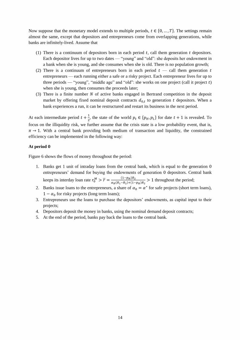
At period 𝟎

Figure 6 shows the flows of money throughout the period:

1. Banks get 1 unit of intraday loans from the central bank, which is equal to the generation 0

entrepreneurs’ demand for buying the endowments of generation 0 depositors. Central bank

keeps its interday loan rate 𝑟0𝑀 > 𝑟 =

(1−𝑝𝐻)𝑅2

𝛼𝐻(𝑅1−𝑅2)+(1−𝑝𝐻)𝑅2> 1 throughout the period;

2. Banks issue loans to the entrepreneurs, a share of 𝛼0 = 𝛼∗ for safe projects (short term loans),

1 − 𝛼0 for risky projects (long term loans);

3. Entrepreneurs use the loans to purchase the depositors’ endowments, as capital input to their

projects;

4. Depositors deposit the money in banks, using the nominal demand deposit contracts;


15

Figure 6 Monetizing the economy at 𝑡 = 0. The arrows show the direction of money flows, and the

numbers indicate the timing of money flows.

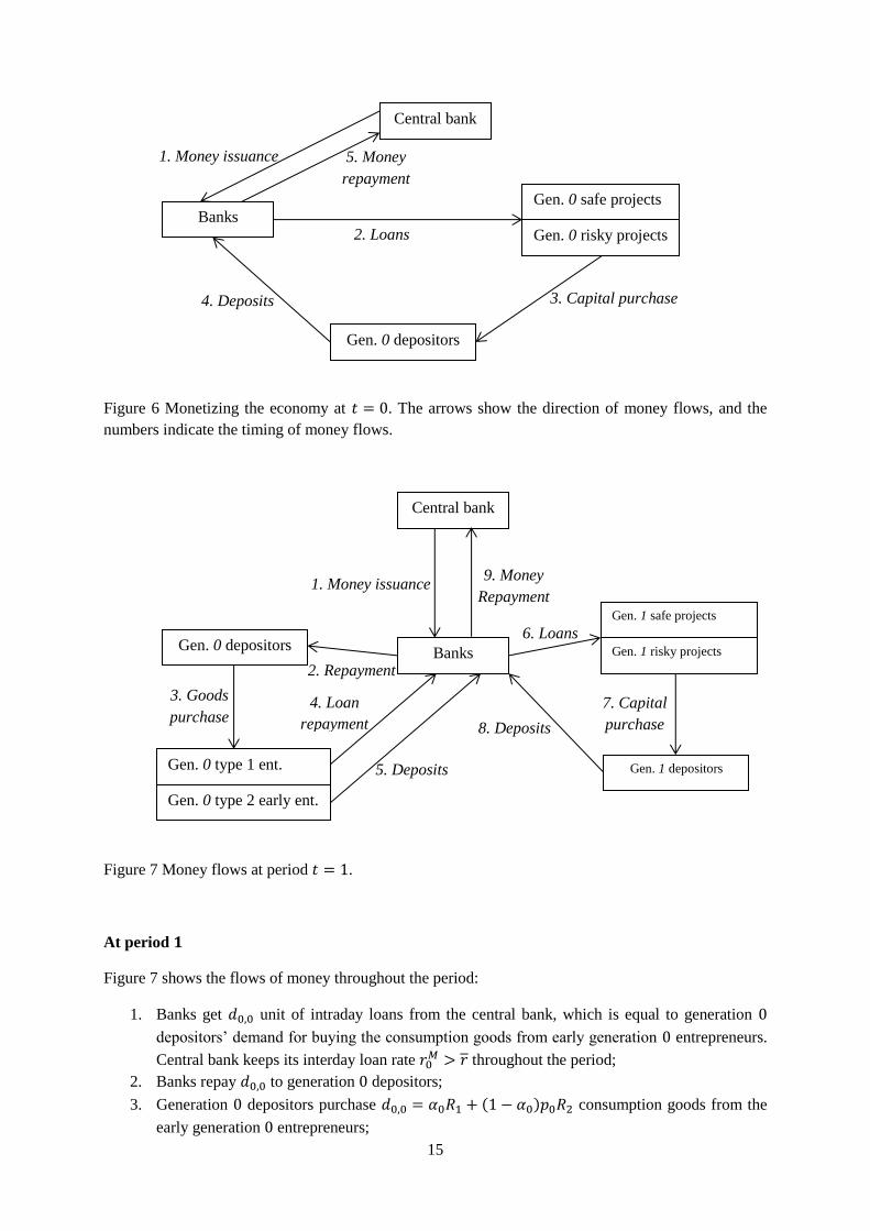
Figure 7 Money flows at period 𝑡 = 1.

At period 𝟏


1. Banks get 𝑑0,0 unit of intraday loans from the central bank, which is equal to generation 0

depositors’ demand for buying the consumption goods from early generation 0 entrepreneurs.

Central bank keeps its interday loan rate 𝑟0𝑀 > 𝑟 throughout the period;

2. Banks repay 𝑑0,0 to generation 0 depositors;

3. Generation 0 depositors purchase 𝑑0,0 = 𝛼0𝑅1 + (1 − 𝛼0)𝑝0𝑅2 consumption goods from the

early generation 0 entrepreneurs;

Central bank

Banks

Gen. 0 type 1 ent.

Gen. 0 type 2 early ent.

Gen. 0 depositors

1. Money issuance

2. Repayment

7. Capital

purchase

5. Deposits

3. Goods

purchase 4. Loan

repayment

Gen. 1 depositors

Gen. 1 safe projects


6. Loans

8. Deposits

9. Money

Repayment

Central bank

Banks Gen. 0 safe projects


Gen. 0 depositors

1. Money issuance

2. Loans

3. Capital purchase 4. Deposits

5. Money

repayment

16

4. Early generation 0 entrepreneurs repay their loans, 𝛾[𝛼0𝑅1 + (1 − 𝛼0)𝑝0𝑅2], to banks, and

5. Deposit (1 − 𝛾)[𝛼0𝑅1 + (1 − 𝛼0)𝑝0𝑅2] in banks;

6. Banks issue loans to generation 1 entrepreneurs, a share of 𝛼1 = 𝛼∗ for safe projects (short

term loans), 1 − 𝛼1 for risky projects (long term loans);

7. Generation 1 entrepreneurs use the loans to purchase generation 1 depositors’ endowments, as

capital input to their projects;

8. Generation 1 depositors deposit the money in banks, using the nominal demand deposit

contracts;


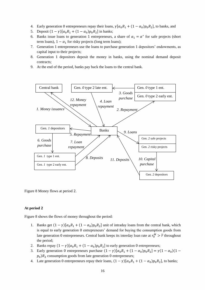
Figure 8 Money flows at period 2.

At period 𝟐


1. Banks get (1 − 𝛾)[𝛼0𝑅1 + (1 − 𝛼0)𝑝0𝑅2] unit of intraday loans from the central bank, which

is equal to early generation 0 entrepreneurs’ demand for buying the consumption goods from

late generation 0 entrepreneurs. Central bank keeps its interday loan rate at 𝑟0𝑀 > 𝑟 throughout

the period;

2. Banks repay (1 − 𝛾)[𝛼0𝑅1 + (1 − 𝛼0)𝑝0𝑅2] to early generation 0 entrepreneurs;

3. Early generation 0 entrepreneurs purchase (1 − 𝛾)[𝛼0𝑅1 + (1 − 𝛼0)𝑝0𝑅2] = 𝛾(1 − 𝛼0)(1 −

𝑝0)𝑅2 consumption goods from late generation 0 entrepreneurs;

4. Late generation 0 entrepreneurs repay their loans, (1 − 𝛾)[𝛼0𝑅1 + (1 − 𝛼0)𝑝0𝑅2], to banks;

Banks

Gen. 1 type 1 ent.


Gen. 1 depositors

5. Repayment

10. Capital

purchase

8. Deposits

6. Goods

purchase 7. Loan

repayment

Gen. 2 depositors

Gen. 2 safe projects


9. Loans

11. Deposits

Gen. 0 type 1 ent.


Gen. 0 type 2 late ent.

2. Repayment

3. Goods

purchase 4. Loan

repayment

Central bank

1. Money issuance

12. Money

repayment

17

5. Banks get 𝑑0,1 − 𝛾(1 − 𝛼0)(1 − 𝑝0)𝑅2 more unit of money of intraday loans from the central

bank and repay 𝑑0,1 to generation 1 depositors;

6. Generation 1 depositors purchase 𝑑0,1 = 𝛼1𝑅1 + (1 − 𝛼1)𝑝1𝑅2 consumption goods from the

early generation 1 entrepreneurs;

7. Early generation 1 entrepreneurs repay their loans, 𝛾[𝛼1𝑅1 + (1 − 𝛼1)𝑝1𝑅2], to banks, and

8. Deposit (1 − 𝛾)[𝛼1𝑅1 + (1 − 𝛼1)𝑝1𝑅2] in banks with gross interest rate 1;

9. Banks issue loans to generation 2 entrepreneurs, a share of 𝛼2 = 𝛼∗ for safe projects (short

term loans), 1 − 𝛼2 for risky projects (long term loans);

10. Generation 2 entrepreneurs use the loans to purchase generation 2 depositors’ endowments, as

capital input to their projects;

11. Generation 2 depositors deposit the money in banks, using the nominal demand deposit

contracts;

12. At the end of the period, banks pay back all the loans to the central bank.

For any period 2 ≤ 𝜏 ≤ 𝑇 after period 2, the intraday money flows are similar as those in period 2, as

long as the economy is in the normal state, with 𝛼𝜏 = 𝛼∗. However, it makes difference when the

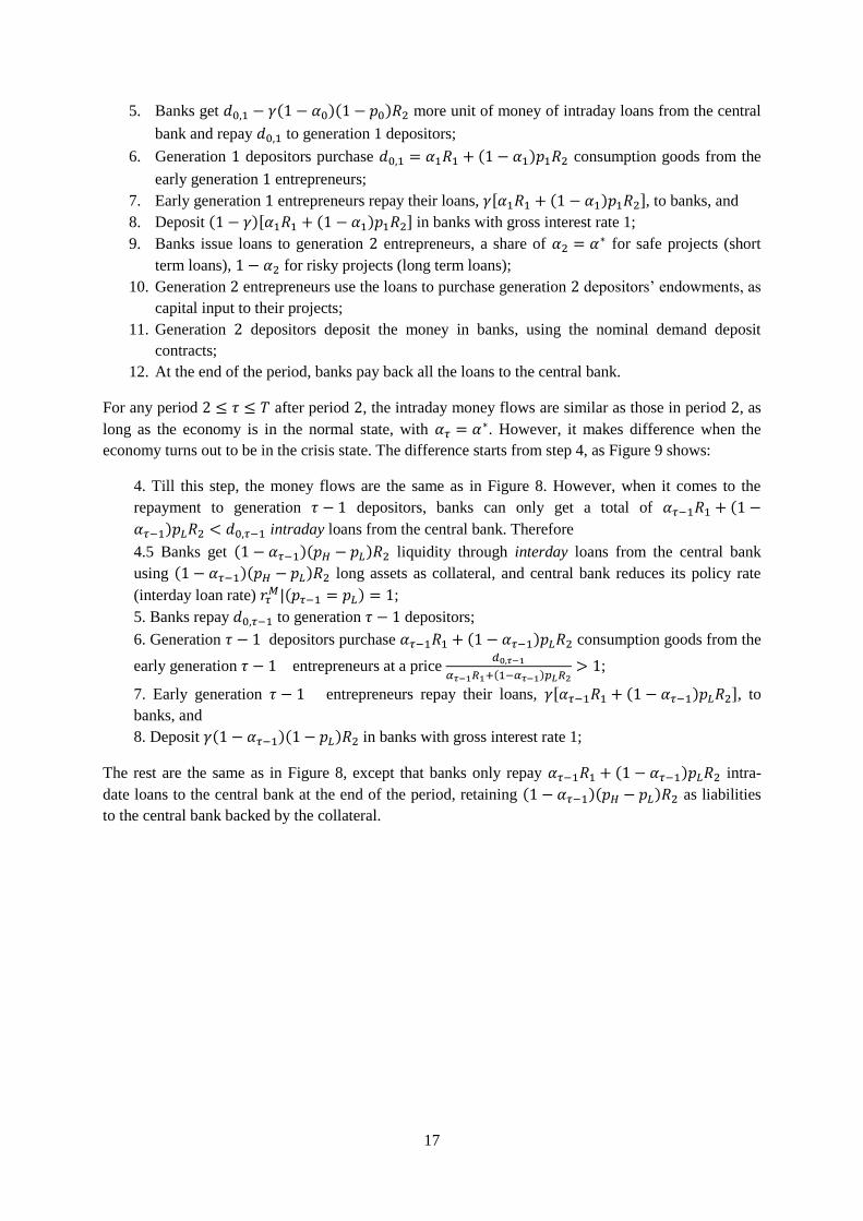
economy turns out to be in the crisis state. The difference starts from step 4, as Figure 9 shows:

4. Till this step, the money flows are the same as in Figure 8. However, when it comes to the

repayment to generation 𝜏 − 1 depositors, banks can only get a total of 𝛼𝜏−1𝑅1 + (1 −

𝛼𝜏−1)𝑝𝐿𝑅2 < 𝑑0,𝜏−1 intraday loans from the central bank. Therefore

4.5 Banks get (1 − 𝛼𝜏−1)(𝑝𝐻 − 𝑝𝐿)𝑅2 liquidity through interday loans from the central bank

using (1 − 𝛼𝜏−1)(𝑝𝐻 − 𝑝𝐿)𝑅2 long assets as collateral, and central bank reduces its policy rate

(interday loan rate) 𝑟𝜏𝑀|(𝑝𝜏−1 = 𝑝𝐿) = 1;

5. Banks repay 𝑑0,𝜏−1 to generation 𝜏 − 1 depositors;

6. Generation 𝜏 − 1 depositors purchase 𝛼𝜏−1𝑅1 + (1 − 𝛼𝜏−1)𝑝𝐿𝑅2 consumption goods from the

early generation 𝜏 − 1 entrepreneurs at a price 𝑑0,𝜏−1

𝛼𝜏−1𝑅1+(1−𝛼𝜏−1)𝑝𝐿𝑅2> 1;

7. Early generation 𝜏 − 1 entrepreneurs repay their loans, 𝛾[𝛼𝜏−1𝑅1 + (1 − 𝛼𝜏−1)𝑝𝐿𝑅2], to

banks, and

8. Deposit 𝛾(1 − 𝛼𝜏−1)(1 − 𝑝𝐿)𝑅2 in banks with gross interest rate 1;

The rest are the same as in Figure 8, except that banks only repay 𝛼𝜏−1𝑅1 + (1 − 𝛼𝜏−1)𝑝𝐿𝑅2 intra-

date loans to the central bank at the end of the period, retaining (1 − 𝛼𝜏−1)(𝑝𝐻 − 𝑝𝐿)𝑅2 as liabilities

to the central bank backed by the collateral.

18

Figure 9 Money flows at any period 𝜏 in the crisis state.

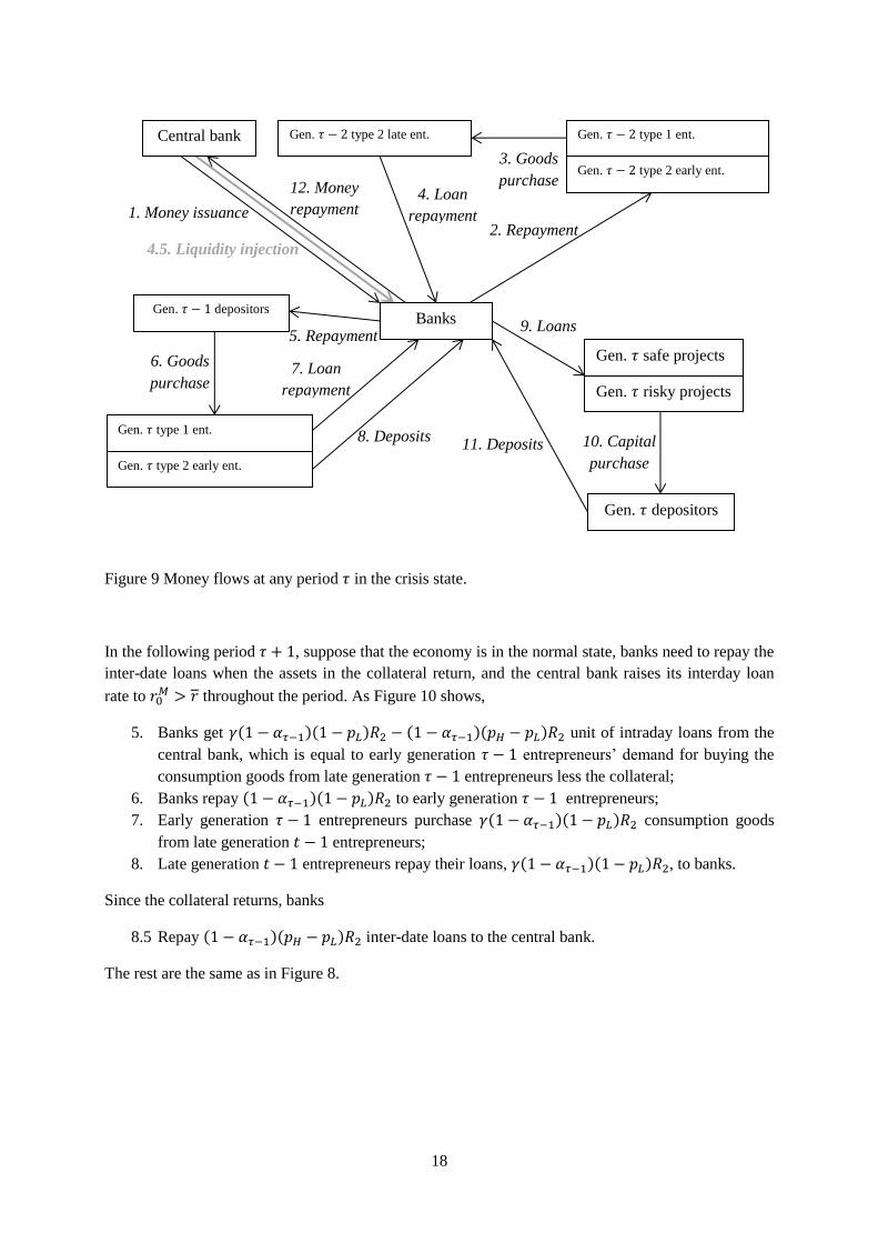
In the following period 𝜏 + 1, suppose that the economy is in the normal state, banks need to repay the

inter-date loans when the assets in the collateral return, and the central bank raises its interday loan

rate to 𝑟0𝑀 > 𝑟 throughout the period. As Figure 10 shows,

5. Banks get 𝛾(1 − 𝛼𝜏−1)(1 − 𝑝𝐿)𝑅2 − (1 − 𝛼𝜏−1)(𝑝𝐻 − 𝑝𝐿)𝑅2 unit of intraday loans from the

central bank, which is equal to early generation 𝜏 − 1 entrepreneurs’ demand for buying the

consumption goods from late generation 𝜏 − 1 entrepreneurs less the collateral;

6. Banks repay (1 − 𝛼𝜏−1)(1 − 𝑝𝐿)𝑅2 to early generation 𝜏 − 1 entrepreneurs;

7. Early generation 𝜏 − 1 entrepreneurs purchase 𝛾(1 − 𝛼𝜏−1)(1 − 𝑝𝐿)𝑅2 consumption goods

from late generation 𝑡 − 1 entrepreneurs;

8. Late generation 𝑡 − 1 entrepreneurs repay their loans, 𝛾(1 − 𝛼𝜏−1)(1 − 𝑝𝐿)𝑅2, to banks.

Since the collateral returns, banks

8.5 Repay (1 − 𝛼𝜏−1)(𝑝𝐻 − 𝑝𝐿)𝑅2 inter-date loans to the central bank.

The rest are the same as in Figure 8.

Gen. 𝜏 type 1 ent.

Gen. 𝜏 type 2 early ent.

Gen. 𝜏 − 1 depositors

5. Repayment

10. Capital

purchase

8. Deposits

6. Goods

purchase 7. Loan

repayment

Gen. 𝜏 depositors

Gen. 𝜏 safe projects

Gen. 𝜏 risky projects

9. Loans

11. Deposits

Gen. 𝜏 − 2 type 1 ent.

Gen. 𝜏 − 2 type 2 early ent.

Gen. 𝜏 − 2 type 2 late ent.

2. Repayment

3. Goods

purchase 4. Loan

repayment 1. Money issuance

12. Money

repayment

Banks

Central bank

4.5. Liquidity injection

19

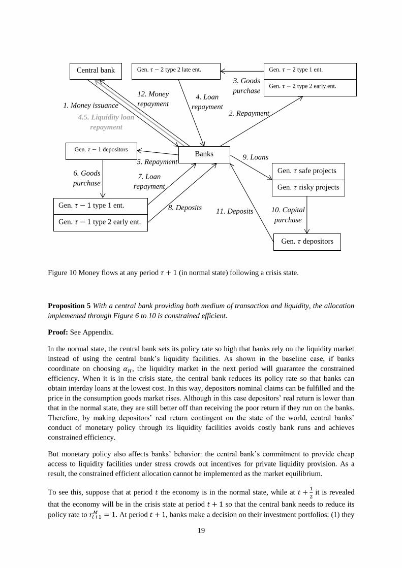
Figure 10 Money flows at any period 𝜏 + 1 (in normal state) following a crisis state.

Proposition 5 With a central bank providing both medium of transaction and liquidity, the allocation

implemented through Figure 6 to 10 is constrained efficient.


In the normal state, the central bank sets its policy rate so high that banks rely on the liquidity market

instead of using the central bank’s liquidity facilities. As shown in the baseline case, if banks

coordinate on choosing 𝛼𝐻, the liquidity market in the next period will guarantee the constrained

efficiency. When it is in the crisis state, the central bank reduces its policy rate so that banks can

obtain interday loans at the lowest cost. In this way, depositors nominal claims can be fulfilled and the

price in the consumption goods market rises. Although in this case depositors’ real return is lower than

that in the normal state, they are still better off than receiving the poor return if they run on the banks.

Therefore, by making depositors’ real return contingent on the state of the world, central banks’

conduct of monetary policy through its liquidity facilities avoids costly bank runs and achieves

constrained efficiency.

But monetary policy also affects banks’ behavior: the central bank’s commitment to provide cheap

access to liquidity facilities under stress crowds out incentives for private liquidity provision. As a

result, the constrained efficient allocation cannot be implemented as the market equilibrium.

To see this, suppose that at period 𝑡 the economy is in the normal state, while at 𝑡 +1

2 it is revealed

that the economy will be in the crisis state at period 𝑡 + 1 so that the central bank needs to reduce its

policy rate to 𝑟𝑡+1𝑀 = 1. At period 𝑡 + 1, banks make a decision on their investment portfolios: (1) they



Gen. 𝜏 − 1 depositors

5. Repayment

10. Capital

purchase

8. Deposits

6. Goods

purchase 7. Loan

repayment

Gen. 𝜏 depositors

Gen. 𝜏 safe projects

Gen. 𝜏 risky projects

9. Loans

11. Deposits



Gen. 𝜏 − 2 type 2 late ent.

2. Repayment

3. Goods

purchase 4. Loan

repayment 1. Money issuance

12. Money

repayment

Banks

Central bank

4.5. Liquidity loan

repayment

20

can either invest 𝛼∗ = 𝛼𝐻 as is suggested by the constrained efficient allocation, (2) or nothing in

liquid assets, 𝛼∗ = 0. Then at period 𝑡 + 2 (most likely, the economy is in the normal state), when the

central bank raises its policy rate to 𝑟𝑡+2𝑀 > 𝑟, if banks opted for (1), they will (be most likely to)

survive since they can get obtain sufficient funding from liquidity market, while if banks opt for (2),

they will become insolvent and experience runs since they cannot raise enough liquidity to fulfill

depositors’ claims. However, if central bank remains its policy rate as 𝑟𝑡+2𝑀 = 1, banks will survive

under both (1) and (2) since they can access to cheap liquidity from central bank.

Ex post, central bank will be indifferent between 𝑟𝑡+2𝑀 > 𝑟 and 𝑟𝑡+2

𝑀 = 1 under (1) since banks receive

the same payoff, 𝛾[𝛼𝐻𝑅1 + (1 − 𝛼𝐻)𝑅2]; under (2), it will prefer 𝑟𝑡+2𝑀 = 1 to 𝑟𝑡+2

𝑀 > 𝑟 to avoid costly

bank runs. However, knowing this, banks will strictly prefer 𝛼∗ = 0 to 𝛼∗ = 𝛼𝐻 at period 𝑡 + 1, since

their payoff is strictly higher, 𝛾𝑅2 > 𝛾[𝛼𝐻𝑅1 + (1 − 𝛼𝐻)𝑅2]. Therefore, in the dynamic consistent

market equilibrium, banks choose 𝛼∗ = 0 and central bank remains 𝑟𝑡𝑀 = 1. By backward induction,

this applies for all 𝑡 ∈ {0, … , 𝑇}.

Notice that in such equilibrium, although depositors receive higher nominal return 𝛾𝑅2 >

𝛾[𝛼𝐻𝑅1 + (1 − 𝛼𝐻)𝑅2], their real consumption 𝛾𝑝𝑡𝑅2 is lower, 𝛾𝑝𝑡𝑅2 < 𝛼𝐻𝑅1 + (1 − 𝛼𝐻)𝑝𝑡𝑅2. This

is due to the fact that all resources are invested in the illiquid assets so that the early return for

depositors is too low. That is, depositors are worse off in the dynamic consistent market equilibrium.

In summary, the dynamic consistent market equilibrium can be characterized in the following

proposition:

Proposition 6 With a central bank providing both medium of transaction and liquidity, the unique

dynamic consistent market equilibrium is characterized by

(1) Banks choose 𝛼𝑡 = 0 and offer nominal deposit contracts 𝑑0𝑡 = 𝛾𝑅2 to depositors, ∀𝑡 ∈

{0, … , 𝑇};

(2) Central bank sets 𝑟𝑡𝑀 = 1, irrespective to the signals observed at 𝑡 −

1

2;

(3) Depositors become worse off than they are under the constrained efficient allocation.


It can be also easily seen that the same conclusion holds even if the time horizon is infinite:

Corollary The dynamic consistent market equilibrium remains the same when 𝑇 → +∞.

6 Discussion

In this section, we discuss two extensions of the model. First, instead of aggregate liquidity shocks, we

assume that liquidity shocks are idiosyncratic to the banks. We show in this case, the market will reach

constrained efficient allocation even in the real economy, while efficiency again breaks down in the

monetary economy. Then we discuss adequate mechanism design to implement constrained efficiency

in the monetary economy. We show that monetary policy rule fails to work due to time inconsistency

problem, and ex ante liquidity requirement is needed to implement the constrained efficient outcome.

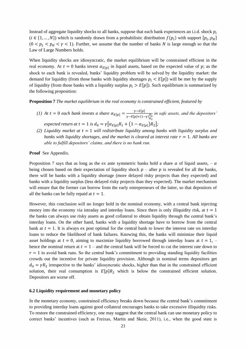
6.1 Idiosyncratic liquidity shocks

21

Instead of aggregate liquidity shocks to all banks, suppose that each bank experiences an i.i.d. shock 𝑝𝑖

(𝑖 ∈ {1, … , 𝑁}) which is randomly drawn from a probabilistic distribution 𝑓(𝑝𝑖) with support [𝑝𝐿 , 𝑝𝐻]

(0 < 𝑝𝐿 < 𝑝𝐻 < 𝛾 < 1). Further, we assume that the number of banks 𝑁 is large enough so that the

Law of Large Numbers holds.

When liquidity shocks are idiosyncratic, the market equilibrium will be constrained efficient in the

real economy. At 𝑡 = 0 banks invest 𝛼𝐸[𝑝] in liquid assets, based on the expected value of 𝑝; as the

shock to each bank is revealed, banks’ liquidity problem will be solved by the liquidity market: the

demand for liquidity (from those banks with liquidity shortages 𝑝𝑖 < 𝐸[𝑝]) will be met by the supply

of liquidity (from those banks with a liquidity surplus 𝑝𝑖 > 𝐸[𝑝]). Such equilibrium is summarized by

the following proposition:

Proposition 7 The market equilibrium in the real economy is constrained efficient, featured by

(1) At 𝑡 = 0 each bank invests a share 𝛼𝐸[𝑝] =𝛾−𝐸[𝑝]

𝛾−𝐸[𝑝]+(1−𝛾)𝑅1𝑅2

in safe assets, and the depositors’

expected return at 𝑡 = 1 is 𝑑0 = 𝛾[𝛼𝐸[𝑝]𝑅1 + (1 − 𝛼𝐸[𝑝])𝑅2];

(2) Liquidity market at 𝑡 = 1 will redistribute liquidity among banks with liquidity surplus and

banks with liquidity shortages, and the market is cleared at interest rate 𝑟 = 1. All banks are

able to fulfill depositors’ claims, and there is no bank run.

Proof See Appendix.

Proposition 7 says that as long as the ex ante symmetric banks hold a share 𝛼 of liquid assets, – 𝛼

being chosen based on their expectation of liquidity shock 𝑝 – after 𝑝 is revealed for all the banks,

there will be banks with a liquidity shortage (more delayed risky projects than they expected) and

banks with a liquidity surplus (less delayed risky projects than they expected). The market mechanism

will ensure that the former can borrow from the early entrepreneurs of the latter, so that depositors of

all the banks can be fully repaid at 𝑡 = 1.

However, this conclusion will no longer hold in the nominal economy, with a central bank injecting

money into the economy via intraday and interday loans. Since there is only illiquidity risk, at 𝑡 = 1

the banks can always use risky assets as good collateral to obtain liquidity through the central bank’s

interday loans. On the other hand, banks with a liquidity shortage have to borrow from the central

bank at 𝑡 = 1. It is always ex post optimal for the central bank to lower the interest rate on interday

loans to reduce the likelihood of bank failures. Knowing this, the banks will minimize their liquid

asset holdings at 𝑡 = 0, aiming to maximize liquidity borrowed through interday loans at 𝑡 = 1, –

hence the nominal return at 𝑡 = 1 – and the central bank will be forced to cut the interest rate down to

𝑟 = 1 to avoid bank runs. So the central bank’s commitment to providing standing liquidity facilities

crowds out the incentive for private liquidity provision. Although in nominal terms depositors get

𝑑0 = 𝛾𝑅2 irrespective to the banks’ idiosyncratic shocks, higher than that in the constrained efficient

solution, their real consumption is 𝐸[𝑝]𝑅2 which is below the constrained efficient solution.

Depositors are worse off.

6.2 Liquidity requirement and monetary policy

In the monetary economy, constrained efficiency breaks down because the central bank’s commitment

to providing interday loans against good collateral encourages banks to take excessive illiquidity risks.

To restore the constrained efficiency, one may suggest that the central bank can use monetary policy to

correct banks’ incentives (such as Freixas, Martin and Skeie, 2011), i.e., when the good state is

22

observed, the policy rate should be prohibitively high so that banks need to borrow from the liquidity

market; while when the bad state is observed, the policy rate should be low enough that banks can

survive through the central bank’s liquidity facilities. Knowing this, banks will have the incentive to

hold liquid assets so that the market mechanism works to allocate liquidity in the good state, and

costly bank runs will be eliminated in the bad state since banks can access the central bank’s liquidity

facilities at low cost.

Unfortunately, such a monetary policy rule fails to work in our dynamic setup since the rule itself is

not credible: If banks do not hold enough liquid assets at 𝑡 = 0, ex post it is always optimal for the

central bank to reduce the policy rate at 𝑡 = 1 to avoid a costly bank run. Knowing this, banks will not

invest in liquid assets at 𝑡 = 0 and the central bank will be forced to set the policy rate at 1 despite the

state of the economy. Owing to the time inconsistency problem, the proposed monetary policy fails to

rescue the economy from the inferior equilibrium.

To avoid supporting banks with excessive investment in illiquid assets, one might suggest that the

central bank should commit to provide interday loans only to those banks who hold sufficient liquid

assets, i.e., 𝛼 ≥ 𝛼∗ in our model. However, such a policy suffers from the same time inconsistency

problem: If one bank doesn’t hold enough liquid assets, 𝛼 < 𝛼∗, at 𝑡 = 0, it is still ex post optimal for

the central bank to allow the bank to access interday loans and avoid costly liquidation from any bank

runs. Therefore, there will be no incentive for banks to hold liquidity in the first place.

Therefore, rather than relying on implausible commitment mechanisms, the solution to fixing the time

inconstancy problem and restoring constrained efficiency in the monetary economy is to combine an

ex ante liquidity requirement with ex post liquidity facilities. In the first place, banks should be

obliged to meet a certain requirement to hold liquid assets (such as the Liquidity Coverage Ratio

defined in Basel III) in the normal time, and when there is a systemic liquidity shortage, the central

bank commits to providing liquidity through interday loans and eliminates bank runs. This deters the

moral hazard that banks are engaged in investing in excessive illiquid assets, raises depositors’

expected real return and restores constrained efficiency.

7 Conclusion

Our paper developed a framework for analyzing the roles of money in banking, both as a medium for

transactions and as bank liquidity. In the model, banks provide a maturity transformation service to

depositors. With fixed deposit contracts and aggregate liquidity risk, the fragile structure of banking

triggers bank runs in the bad state, leading to socially costly liquidation.

Ideally, in a monetary economy with nominal deposit contracts, a central bank conducting active

monetary policy can eliminate such costly liquidation and replicate the first best solution. Money is

issued by the central bank through (1) intraday loans to the bank, as a medium facilitating transaction,

and (2) interday loans to banks, or standing liquidity facilities, to accommodate their demand for

liquidity, using illiquid long assets as collateral. In good times, banks can borrow from the liquidity

market to meet depositors’ demand; while in bad times when banks suffer from liquidity shortage, the

central bank will inject liquidity to the market through liquidity facilities, making sure banks can still

fulfill their nominal deposit contracts. The central bank’s policy rate should be high in good times to

encourage the efficient market outcome, while it should be low in bad times to avoid runs.

Unfortunately, such a scheme cannot be an equilibrium market outcome. Absent liquidity regulation,

banks always have incentives to invest excessively in illiquid assets and obtain liquidity from the

23

central bank to maximize depositors’ nominal return. Banks are more likely to have liquidity shortages

even in good times. So the central bank will be forced to reduce its policy rate to prevent bank failure.

As a result, the economy will end up in an inferior equilibrium: banks overinvest in illiquid assets, the

central bank has to keep policy rate low, and depositors are worse off through lower real consumption.

We show that using interest rate rules to deter banks’ excessive risk taking is not credible for

implementing the constrained efficient allocation, because of a time inconsistency problem: Once

banks engage in excessive liquidity risks ex ante, it is always ex post optimal for the central bank to

reduce the interest rate. An additional instrument, such as imposing a liquidity coverage requirement

ex ante, is needed to restore efficiency in the monetary equilibrium.

Appendix

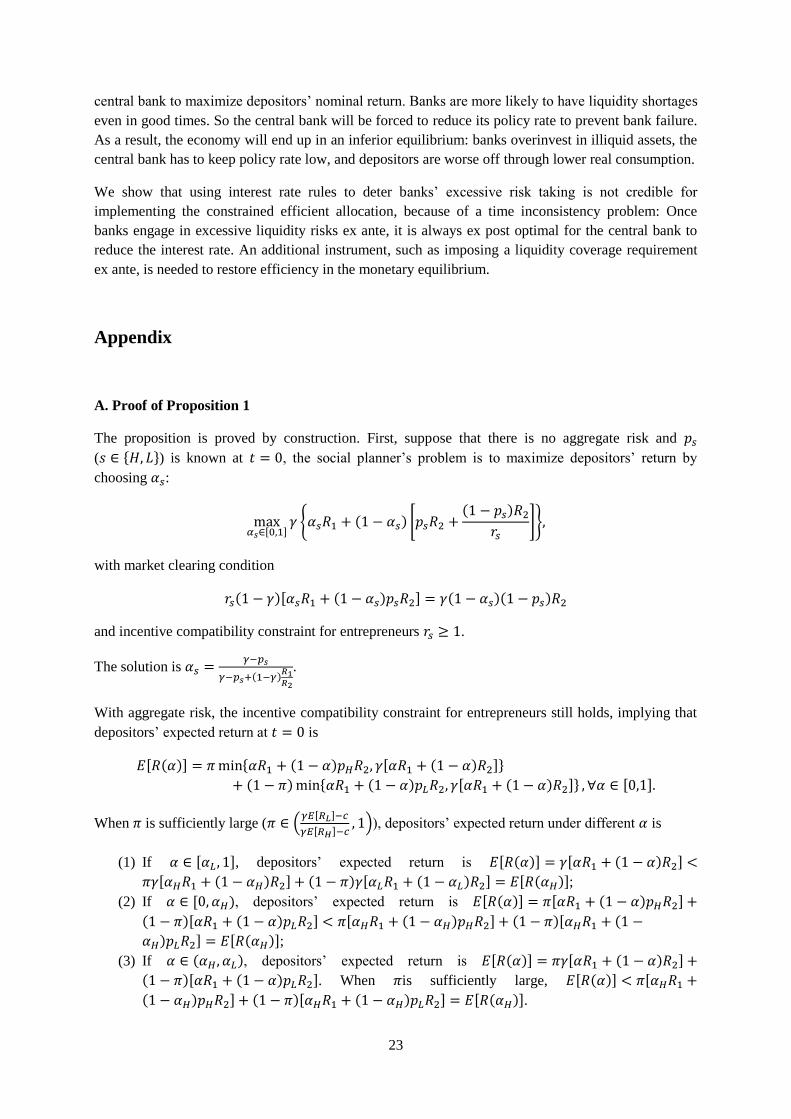
A. Proof of Proposition 1

The proposition is proved by construction. First, suppose that there is no aggregate risk and 𝑝𝑠

(𝑠 ∈ {𝐻, 𝐿}) is known at 𝑡 = 0, the social planner’s problem is to maximize depositors’ return by

choosing 𝛼𝑠:

max𝛼𝑠∈[0,1]

𝛾 {𝛼𝑠𝑅1 + (1 − 𝛼𝑠) [𝑝𝑠𝑅2 +(1 − 𝑝𝑠)𝑅2

𝑟𝑠]},

with market clearing condition

𝑟𝑠(1 − 𝛾)[𝛼𝑠𝑅1 + (1 − 𝛼𝑠)𝑝𝑠𝑅2] = 𝛾(1 − 𝛼𝑠)(1 − 𝑝𝑠)𝑅2

and incentive compatibility constraint for entrepreneurs 𝑟𝑠 ≥ 1.

The solution is 𝛼𝑠 =𝛾−𝑝𝑠

𝛾−𝑝𝑠+(1−𝛾)𝑅1𝑅2

.

With aggregate risk, the incentive compatibility constraint for entrepreneurs still holds, implying that

depositors’ expected return at 𝑡 = 0 is

𝐸[𝑅(𝛼)] = 𝜋 min{𝛼𝑅1 + (1 − 𝛼)𝑝𝐻𝑅2, 𝛾[𝛼𝑅1 + (1 − 𝛼)𝑅2]}

+ (1 − 𝜋) min{𝛼𝑅1 + (1 − 𝛼)𝑝𝐿𝑅2, 𝛾[𝛼𝑅1 + (1 − 𝛼)𝑅2]} , ∀𝛼 ∈ [0,1].

When 𝜋 is sufficiently large (𝜋 ∈ (𝛾𝐸[𝑅𝐿]−𝑐

𝛾𝐸[𝑅𝐻]−𝑐, 1)), depositors’ expected return under different 𝛼 is

(1) If 𝛼 ∈ [𝛼𝐿 , 1], depositors’ expected return is 𝐸[𝑅(𝛼)] = 𝛾[𝛼𝑅1 + (1 − 𝛼)𝑅2] <

𝜋𝛾[𝛼𝐻𝑅1 + (1 − 𝛼𝐻)𝑅2] + (1 − 𝜋)𝛾[𝛼𝐿𝑅1 + (1 − 𝛼𝐿)𝑅2] = 𝐸[𝑅(𝛼𝐻)];

(2) If 𝛼 ∈ [0, 𝛼𝐻), depositors’ expected return is 𝐸[𝑅(𝛼)] = 𝜋[𝛼𝑅1 + (1 − 𝛼)𝑝𝐻𝑅2] +

(1 − 𝜋)[𝛼𝑅1 + (1 − 𝛼)𝑝𝐿𝑅2] < 𝜋[𝛼𝐻𝑅1 + (1 − 𝛼𝐻)𝑝𝐻𝑅2] + (1 − 𝜋)[𝛼𝐻𝑅1 + (1 −

𝛼𝐻)𝑝𝐿𝑅2] = 𝐸[𝑅(𝛼𝐻)];

(3) If 𝛼 ∈ (𝛼𝐻 , 𝛼𝐿), depositors’ expected return is 𝐸[𝑅(𝛼)] = 𝜋𝛾[𝛼𝑅1 + (1 − 𝛼)𝑅2] +

(1 − 𝜋)[𝛼𝑅1 + (1 − 𝛼)𝑝𝐿𝑅2]. When 𝜋is sufficiently large, 𝐸[𝑅(𝛼)] < 𝜋[𝛼𝐻𝑅1 +

(1 − 𝛼𝐻)𝑝𝐻𝑅2] + (1 − 𝜋)[𝛼𝐻𝑅1 + (1 − 𝛼𝐻)𝑝𝐿𝑅2] = 𝐸[𝑅(𝛼𝐻)].

24

Therefore, when 𝜋 is sufficiently large, choosing 𝛼𝐻 maximizes depositors’ expected return.

B. Proof of Proposition 2

To show that the allocation is the market equilibrium in the real economy, we need to show that the

allocation is feasible and it is not profitable for any bank to deviate unilaterally.

If all banks choose 𝛼∗ = 𝛼𝐻, when 𝑝𝐻 is revealed, depositors will get a maximized return, 𝑑0∗ =

𝛾𝐸[𝑅𝐻], and this is exactly the solution to the planner’s problem. However, when 𝑝𝐿 is revealed at

𝑡 =1

2, banks can at most collect 𝛼𝐻𝑅1 + (1 − 𝛼𝐻)𝑝𝐿𝑅2 < 𝑑0

∗ from early entrepreneurs and liquidity

market at 𝑡 = 1. This triggers a bank run at 𝑡 =1

2, forcing banks to liquidate both safe and risky

projects for an inferior return 𝑐. Therefore, depositors’ expected return at 𝑡 = 0 is 𝛾𝜋𝐸[𝑅𝐻] +

(1 − 𝜋)𝑐 < 𝛾𝜋𝐸[𝑅𝐻] + (1 − 𝜋)[𝛼𝐻𝑅1 + (1 − 𝛼𝐻)𝑝𝐿𝑅2] = 𝐸[𝑅(𝛼𝐻)], inferior to the planner’s

solution.

Suppose one bank 𝑖 chooses 𝛼𝑖 ≠ 𝛼𝐻:

(1) If 𝛼𝑖 < 𝛼𝐻, when 𝑝𝐻 is revealed, the interest rate in liquidity market at 𝑡 = 1 is determined by

𝑟′{(1 − 𝛾)[𝛼𝑖𝑅1 + (1 − 𝛼𝑖)𝑝𝐻𝑅2] + (𝑁 − 1)(1 − 𝛾)[𝛼𝐻𝑅1 + (1 − 𝛼𝐻)𝑝𝐻𝑅2]}

= 𝛾(1 − 𝛼𝑖)(1 − 𝑝𝐻)𝑅2 + (𝑁 − 1)𝛾(1 − 𝛼𝐻)(1 − 𝑝𝐻)𝑅2.

Remember that in the planner’s problem, the equilibrium interest rate is determined by

𝑟𝐻(1 − 𝛾)[𝛼𝐻𝑅1 + (1 − 𝛼𝐻)𝑝𝐻𝑅2] = 𝛾(1 − 𝛼𝐻)(1 − 𝑝𝐻)𝑅2,

and 𝑟𝐻 = 1. Therefore, 𝑟′ > 1. For the non-deviators, their return at 𝑡 = 1 becomes

𝛾 {𝛼𝐻𝑅1 + (1 − 𝛼𝐻) [𝑝𝐻𝑅2 +(1 − 𝑝𝐻)𝑅2

𝑟′]} < 𝑑0

∗

When 𝑝𝐿 is revealed, both deviator and non-deviators will experience runs.

Knowing that non-deviators will not even be able to meet the contracted 𝑑0∗ at 𝑡 = 1, the

depositors will only deposit at bank 𝑖 at 𝑡 = 0. If so, the deposit return that bank 𝑖 can offer is

𝑑0𝑖 = 𝛼𝑖𝑅1 + (1 − 𝛼𝑖)𝑝𝐻𝑅2 < 𝑑0∗ ,

implying that the deviator becomes worse off;

(2) If 𝛼𝑖 > 𝛼𝐻, when 𝑝𝐻 is revealed, the aggregate liquidity supply at 𝑡 = 1 exceeds aggregate

liquidity demand because

(1 − 𝛾)[𝛼𝑖𝑅1 + (1 − 𝛼𝑖)𝑝𝐻𝑅2] + (𝑁 − 1)(1 − 𝛾)[𝛼𝐻𝑅1 + (1 − 𝛼𝐻)𝑝𝐻𝑅2]

> 𝑁(1 − 𝛾)[𝛼𝐻𝑅1 + (1 − 𝛼𝐻)𝑝𝐻𝑅2] = 𝑁𝛾(1 − 𝛼𝐻)(1 − 𝑝𝐻)𝑅2,

Implying that the liquidity market interest rate remains at 𝑟 = 1 and non-deviators are able to

meet 𝑑0∗ at 𝑡 = 1. However, the deviator’s return at 𝑡 = 1 is

𝑑0𝑖 = 𝛾[𝛼𝑖𝑅1 + (1 − 𝛼𝑖)𝑅2] < 𝑑0∗ .

When 𝑝𝐿 is revealed, non-deviator banks experience liquidity shortages and bid up the

liquidity market interest rate. As a result, even if the deviator invests more in liquid assets, it

cannot meet the deposit contract either. Therefore, both deviator and non-deviators will

experience runs.

25

Since the expected return from non-deviator banks is higher than that from the deviator,

implying that the deviator will not get any deposit at 𝑡 = 0 and is hence worse off.

Therefore the suggested allocation is indeed the market equilibrium in real economy.

C. Proof of Proposition 3

By investing a share 𝛼∗ = 𝛼𝐻 =𝛾−𝑝𝐻


at 𝑡 = 0 on the safe projects, at 𝑡 = 1

(1) If it is in the good state, banks collect 𝛾[𝛼𝐻𝑅1 + (1 − 𝛼𝐻)𝑝𝐻𝑅2] real return from early

entrepreneurs. Using the late projects (1 − 𝛼𝐻)(1 − 𝑝𝐻)𝑅2 = (1 − 𝛾)[𝛼𝐻𝑅1 + (1 −

𝛼𝐻)𝑝𝐻𝑅2] as collateral, the banks are able to borrow (1 − 𝛾)[𝛼𝐻𝑅1 + (1 − 𝛼𝐻)𝑝𝐻𝑅2] from

the early entrepreneurs at the interest rate 𝑟𝑔 = 1. The central bank’s aggregate supply of

money to the banks through intraday loans is thus 𝑀𝑔 = 𝛾[𝛼𝐻𝑅1 + (1 − 𝛼𝐻)𝑝𝐻𝑅2] +

(1 − 𝛾)[𝛼𝐻𝑅1 + (1 − 𝛼𝐻)𝑝𝐻𝑅2] = 𝛼𝐻𝑅1 + (1 − 𝛼𝐻)𝑝𝐻𝑅2 = 𝛾[𝛼𝐻𝑅1 + (1 − 𝛼𝐻)𝑅2] = 𝑑0,

the same as the depositors’ nominal return. On the other hand, the aggregate output at 𝑡 = 1 is

𝑌𝑔 = 𝛼𝐻𝑅1 + (1 − 𝛼𝐻)𝑝𝐻𝑅2, the aggregate demand for money in goods transaction 𝑃𝑔𝑌𝑔 =

𝑀𝑔 implies that the price level is 𝑃𝑔 = 1;

(2) If it is in the bad state, banks collect 𝛾[𝛼𝐻𝑅1 + (1 − 𝛼𝐻)𝑝𝐿𝑅2] real return from early

entrepreneurs. Using (1 − 𝛾)[𝛼𝐻𝑅1 + (1 − 𝛼𝐻)𝑝𝐿𝑅2] late projects as collateral, the banks are

able to borrow (1 − 𝛾)[𝛼𝐻𝑅1 + (1 − 𝛼𝐻)𝑝𝐿𝑅2] from the early entrepreneurs at the interest

rate 𝑟𝑏 = 1. The central bank’s aggregate supply of money to the banks through intraday loans

is thus 𝛾[𝛼𝐻𝑅1 + (1 − 𝛼𝐻)𝑝𝐿𝑅2] + (1 − 𝛾)[𝛼𝐻𝑅1 + (1 − 𝛼𝐻)𝑝𝐿𝑅2] = 𝛼𝐻𝑅1 +

(1 − 𝛼𝐻)𝑝𝐿𝑅2. The banks can further borrow from the central bank at 𝑟𝑀 = 1 through

interday loans, using the rest of late projects 𝛾(1 − 𝛼𝐻)(𝑝𝐻 − 𝑝𝐿)𝑅2 as collateral. In the end,

the depositors’ nominal return, or aggregate money supply in the economy, is 𝑀𝑏 =

𝛾[𝛼𝐻𝑅1 + (1 − 𝛼𝐻)𝑝𝐿𝑅2] + (1 − 𝛾)[𝛼𝐻𝑅1 + (1 − 𝛼𝐻)𝑝𝐿𝑅2] + 𝛾(1 − 𝛼𝐻)(𝑝𝐻 − 𝑝𝐿)𝑅2 =

𝛼𝐻𝑅1 + (1 − 𝛼𝐻)𝑝𝐻𝑅2 = 𝛾[𝛼𝐻𝑅1 + (1 − 𝛼𝐻)𝑅2] = 𝑑0, the same as that is promised in the

deposit contracts. On the other hand, the aggregate output at 𝑡 = 1 is now 𝑌𝑏 = 𝛼𝐻𝑅1 +

(1 − 𝛼𝐻)𝑝𝐿𝑅2, the aggregate demand for money in goods transaction 𝑃𝑏𝑌𝑏 = 𝑀𝑏 implies that

the price level is 𝑃𝑏 =𝑑0

𝛼𝐻𝑅1+(1−𝛼𝐻)𝑝𝐿𝑅2=

𝛼𝐻𝑅1+(1−𝛼𝐻)𝑝𝐻𝑅2

𝛼𝐻𝑅1+(1−𝛼𝐻)𝑝𝐿𝑅2> 1.

Furthermore, there will be no bank run in such a decentralized monetary economy. In the good state,

the depositors receive 𝑑0 nominal repayment and the same amount of real consumption, so there will

be no incentive to run on the bank. In the bad state, the depositors get at most 𝛼𝐻𝑅1 + (1 −

𝛼𝐻)𝑝𝐿𝑅2 < 𝑑0 consumption; however, if they run on the bank at 𝑡 =1

2, they can only get 𝑐 < 1 <

𝛼𝐻𝑅1 + (1 − 𝛼𝐻)𝑝𝐿𝑅2 real consumption. Therefore, they will prefer not to run on the bank and wait

instead to get 𝑑0 nominal repayment at 𝑡 = 1.

The banks’ nominal repayment to depositors at 𝑡 = 1 is 𝑑𝑠 = 𝛾 {𝛼𝐻𝑅1 + (1 − 𝛼𝐻) [𝑝𝑠𝑅2 +(1−𝑝𝑠)𝑅2

𝑟𝑠]},

in which 𝑟𝑠 is the rate of the banks’ borrowing from entrepreneurs and / or the central bank in the state

𝑠 ∈ {𝐻, 𝐿}:

(1) In the bad state, if the banks only borrow from early entrepreneurs, market clearing condition

𝑟𝐿(1 − 𝛾)[𝛼𝐻𝑅1 + (1 − 𝛼𝐻)𝑝𝐿𝑅2] = 𝛾(1 − 𝛼𝐻)(1 − 𝑝𝐿)𝑅2

implies that 𝑟𝐿 > 1, hence 𝑑𝐿 < 𝑑0. However, if the central bank commits to setting 𝑟𝑀 = 1

for its interday loans so that banks can borrow from both early entrepreneurs and the central

26

bank, depositors’ nominal repayment will be 𝑑𝐿 = 𝑑0 since 𝑟𝐿 = 𝑟𝑀 = 1. The constrained

efficiency is achieved;

(2) In the good state, if the central bank’s policy rate is 𝑟𝑔𝑀 =

(1−𝑝𝐻)𝑅2

𝛼∗(𝑅1−𝑅2)+(1−𝑝𝐻)𝑅2> 1, the banks

will only borrow from the early entrepreneurs at the rate 𝑟𝐻 =𝛾(1−𝛼𝐻)(1−𝑝𝐻)𝑅2

(1−𝛾)[𝛼𝐻𝑅1+(1−𝛼𝐻)𝑝𝐻𝑅2]= 1.

The depositors’ nominal repayment is therefore 𝑑𝐻 = 𝑑0 and the constrained efficiency is

achieved.

D. Proof of Proposition 4

The proposition is proved by backward induction. The game consists of two subgames:

(1) At 𝑡 = 1, for the banks with strategic profile (𝛼, 𝑑0), the central bank needs to set its policy

rate 𝑟𝑆𝑀 that maximizes the banks’ return in the state 𝑠 ∈ {𝐻, 𝐿}, i.e.

max𝑟𝑆

𝑀𝛾 {𝛼𝑅1 + (1 − 𝛼) [𝑝𝑠𝑅2 +

(1 − 𝑝𝑠)𝑅2

𝑟𝑠]}

in which 𝑟𝑠 = min{𝑟𝑠0, 𝑟𝑆

𝑀}. The banks may borrow from the entrepreneurs at the rate 𝑟𝑠0,

which is determined by 𝑟𝑠0 =

𝛾(1−𝛼)(1−𝑝𝑠)𝑅2

(1−𝛾)[𝛼𝑅1+(1−𝛼)𝑝𝑠𝑅2], and 𝑟𝑠

0 ≥ 1 to allow entrepreneurs to

participate. Obviously, the central bank’s optimal policy rate is 𝑟𝑆𝑀 = 1 irrespective of the

state;

(2) Known that 𝑟𝑠 = 𝑟𝑆𝑀 = 1 at 𝑡 = 1, the banks’ problem at 𝑡 = 0 is to choose the strategic

profile (𝛼, 𝑑0) that maximizes depositors’ nominal return, i.e.

max(𝛼,𝑑0)

𝑑0 = 𝛾 {𝛼𝑅1 + (1 − 𝛼) [𝑝𝑠𝑅2 +(1 − 𝑝𝑠)𝑅2

𝑟𝑠]} = 𝛾{𝛼𝑅1 + (1 − 𝛼)𝑅2}.

Since 𝑅2 > 𝑅1, it is optimal to set 𝛼 = 0 and 𝑑0 = 𝛾𝑅2.

As for the aggregate real output and price level,

(1) In the good state, banks collect 𝛾𝑝𝐻𝑅2 real return from early entrepreneurs. Using part of the

late projects (1 − 𝛾)𝑝𝐻𝑅2 as collateral, the banks are able to borrow (1 − 𝛾)𝑝𝐻𝑅2 from the

early entrepreneurs at the interest rate 𝑟′𝑔 = 1. The central bank’s aggregate supply of money

to the banks through intraday loans is thus 𝛾𝑝𝐻𝑅2 + (1 − 𝛾)𝑝𝐻𝑅2 = 𝑝𝐻𝑅2, The banks can

further borrow from the central bank at 𝑟𝑀 = 1 through interday loans, using the rest of late

projects 𝛾(1 − 𝑝𝐻)𝑅2 − (1 − 𝛾)𝑝𝐻𝑅2 = (𝛾 − 𝑝𝐻)𝑅2 as collateral. In the end, the depositors’

nominal return, or aggregate money supply in the economy, is 𝑀′𝑔 = 𝛾𝑝𝐻𝑅2 + 𝛾(1 −

𝑝𝐻)𝑅2 = 𝛾𝑅2 = 𝑑0, the same as that is promised in the deposit contracts. On the other hand,

the aggregate output at 𝑡 = 1 is now 𝑌′𝑔 = 𝑝𝐻𝑅2, the aggregate demand for money in goods

transaction 𝑃′𝑔𝑌′𝑔 = 𝑀′𝑔 implies that the price level is 𝑃′𝑔 =𝛾

𝑝𝐻> 𝑃𝑔 = 1;

(2) In the bad state, banks collect 𝛾𝑝𝐿𝑅2 real return from early entrepreneurs. Using part of the

late projects (1 − 𝛾)𝑝𝐿𝑅2 as collateral, the banks are able to borrow (1 − 𝛾)𝑝𝐿𝑅2 from the

early entrepreneurs at the interest rate 𝑟′𝑏 = 1. The central bank’s aggregate supply of money

to the banks through intraday loans is thus 𝛾𝑝𝐿𝑅2 + (1 − 𝛾)𝑝𝐿𝑅2 = 𝑝𝐿𝑅2, The banks can

further borrow from the central bank at 𝑟𝑀 = 1 through interday loans, using the rest of late

projects 𝛾(1 − 𝑝𝐿)𝑅2 − (1 − 𝛾)𝑝𝐿𝑅2 = (𝛾 − 𝑝𝐿)𝑅2 as collateral. In the end, the depositors’

nominal return, or aggregate money supply in the economy, is 𝑀′𝑏 = 𝛾𝑝𝐿𝑅2 + 𝛾(1 −

𝑝𝐿)𝑅2 = 𝛾𝑅2 = 𝑑0, the same as that is promised in the deposit contracts. On the other hand,

the aggregate output at 𝑡 = 1 is now 𝑌′𝑏 = 𝑝𝐿𝑅2, the aggregate demand for money in goods

27

transaction 𝑃′𝑏𝑌′𝑏 = 𝑀′𝑏 implies that the price level is 𝑃′𝑏 =𝛾

𝑝𝐿=

𝛾[𝛼𝐻𝑅1+(1−𝛼𝐻)𝑅2]

𝑝𝐿[𝛼𝐻𝑅1+(1−𝛼𝐻)𝑅2]=


𝑝𝐿[𝛼𝐻𝑅1+(1−𝛼𝐻)𝑅2]>


𝛼𝐻𝑅1+(1−𝛼𝐻)𝑝𝐿𝑅2= 𝑃𝑏.

E. Proof of Proposition 5

Since the planner’s problem is symmetric at any 𝑡, it is the same as the one in the static model

characterized in section 2. The allocation implemented through Figure 6 to 10 is the same as in

Proposition 1, therefore, it replicates the constrained efficient solution.

F. Proof of Proposition 6

The proposition is proved by backward induction. At any period 𝑡

(1) If the banks choose (𝛼∗, 𝑑0∗)

a. If the central bank chooses 𝑟𝑡+1𝑀 = 1, banks’ nominal return is 𝑑0

∗ despite the state at

𝑡 + 1;

b. If the central bank chooses 𝑟𝑡+1𝑀 > 1, banks’ nominal return is 𝑑0

∗ in the good state,

while in the bad state the maximal nominal return is 𝛾 [𝛼∗𝑅1 + (1 − 𝛼∗)𝑝𝐿𝑅1 +

(1−𝛼∗)(1−𝑝𝐿)𝑅1

𝑟𝑡+1𝑀 ] < 𝑑0

∗ so that banks will experience runs. Banks’ expected nominal

return at 𝑡 is therefore 𝜋𝑑0∗ + (1 − 𝜋)𝑐 < 𝑑0

∗;

(2) If the banks choose (�̃�, �̃�0) ≠ (𝛼∗, 𝑑0∗)

a. If the central bank chooses 𝑟𝑡+1𝑀 = 1, banks’ nominal return is �̃�0 = 𝛾[�̃�𝑅1 +

(1 − �̃�)𝑅2] which is maximized at �̃� = 0. In this case, �̃�0 = 𝛾𝑅2 > 𝑑0∗;

b. If the central bank chooses 𝑟𝑡+1𝑀 > 1, banks’ nominal return is , �̃�0 = max {�̃�𝑅1 +

(1 − �̃�)𝑝𝑅2, 𝛾 [�̃�𝑅1 + (1 − �̃�)𝑝𝑅1 +(1−�̃�)(1−𝑝)𝑅1

𝑟𝑡+1𝑀 ]} < 𝑑0

∗.

The unique subgame perfect equilibrium is that bankers choose 𝛼 = 0, 𝑑0 = 𝛾𝑅2 at 𝑡, and the central

bank stays with 𝑟𝑡+1𝑀 = 1, irrespective of the signal observed at 𝑡 + 1.5. However, the real return the

investors receive is 𝑝𝑅2 < 𝑑0∗.

G. Proof of Proposition 7

Under idiosyncratic liquidity shocks, the social planner’s problem is to maximize depositors’ expected

return by choosing 𝛼𝑖 for bank 𝑖 at 𝑡 = 0:

max𝛼𝑖∈[0,1]

𝑑0 = 𝐸0 [𝛾 {𝛼𝑖𝑅1 + (1 − 𝛼𝑖) [𝑝𝑖𝑅2 +(1 − 𝑝𝑖)𝑅2

𝑟]}],

with market clearing condition

𝑟 ∑(1 − 𝛾)[𝛼𝑖𝑅1 + (1 − 𝛼𝑖)𝑝𝑖𝑅2]

𝑁

𝑖=1

= ∑ 𝛾(1 − 𝛼𝑖)(1 − 𝑝𝑖)𝑅2

𝑁

𝑖=1

and incentive compatibility constraint for entrepreneurs 𝑟 ≥ 1.

28

The solution is 𝛼𝑖 =𝛾−𝐸[𝑝]

𝛾−𝐸[𝑝]+(1−𝛾)𝑅1𝑅2

, 𝑑0 = 𝛾[𝛼𝐸[𝑝]𝑅1 + (1 − 𝛼𝐸[𝑝])𝑅2] and 𝑟 = 1.

In the market equilibrium, bank 𝑖’s problem is to maximize its depositors’ expected return by choosing

𝛼𝑖 at 𝑡 = 0:

max𝛼𝑖∈[0,1]

𝑑0 = 𝐸0 [𝛾 {𝛼𝑖𝑅1 + (1 − 𝛼𝑖) [𝑝𝑖𝑅2 +(1 − 𝑝𝑖)𝑅2

𝑟]}],

taking into account the market clearing condition

𝑟 ∑(1 − 𝛾)[𝛼𝑖𝑅1 + (1 − 𝛼𝑖)𝑝𝑖𝑅2]

𝑁

𝑖=1

= ∑ 𝛾(1 − 𝛼𝑖)(1 − 𝑝𝑖)𝑅2

𝑁

𝑖=1

and incentive compatibility constraint for entrepreneurs 𝑟 ≥ 1.

Since all the banks are ex ante symmetric, bank 𝑖’s problem in the market equilibrium is the same as

the social planner’s problem, the solution should be the same and constrained efficient. In addition,

depositors’ return 𝑑0 doesn’t depend on the bank’s realized liquidity shock 𝑝𝑖, therefore, there is no

bank run.

References

Allen, F., Carletti, E. and Gale, D. (2009), Interbank market liquidity and central bank intervention,

Journal of Monetary Economics 56, 639-652.

Allen, F., Carletti, E. and Gale, D. (2014), Money, financial stability and efficiency, Journal of

Economic Theory 149, 100-127.

Diamond, D. and Rajan, R. (2001), Liquidity risk, liquidity creation and financial fragility: a theory of

banking, Journal of Political Economy 109, 2431-2465.

Diamond, D. and Rajan, R. (2006), Money in a theory of banking, American Economic Review 96, 30-

53.

Diamond, D. W. and Rajan, R. G. (2012), Illiquid banks, financial stability, and interest rate policy,

Journal of Political Economy 120, 552-591.

Freixas, X., Martin, A. and Skeie, D. (2011), Bank liquidity, interbank markets, and monetary policy,

Review of Financial Studies 24, 2656-2692.

Hart, O. and Moore, J. (1994), A Theory of debt based on the inalienability of human capital,

Quarterly Journal of Economics 109, 841-79.

Skeie, D. (2008), Banking with nominal deposits and inside money, Journal of Financial

Intermediation 17, 562-584.

money in the equilibrium of banking · [email protected] abstract in most banking models, money is...

Documents