multilevel scheduling of computations
TRANSCRIPT
Multilevel Scheduling of Computations
on Parallel Large-scale Systems
Inauguraldissertation
zur
Erlangung der Würde eines Doktors der Philosophie
vorgelegt der
Philosophisch-Naturwissenschaftlichen Fakultät
der Universität Basel
von Ahmed Hamdy Mohamed Eleliemy
Basel, 2021
Originaldokument gespeichert auf dem Dokumentenserverder Universität Basel
edoc.unibas.ch
Genehmigt von der Philosophisch-Naturwissenschaftlichen Fakultätauf Antrag von
Prof. Dr. Florina M. Ciorba, First SupervisorProf. Dr. Heiko Schuldt, Second SupervisorProf. Dr. Wolfgang E. Nagel, External Expert
Basel, den 02.03.2021
Prof. Dr. Marcel Mayor, Dekan


to the soul of my parents

Abstract
Computational scientists are eager to utilize computing resources to executetheir applications to advance their understanding of various complex phenom-ena. This eagerness drives the rapid technological development in high per-formance computing (HPC). Modern HPC systems exhibit rapid growth in thenumber of cores per computing node and the number of computing nodes persystem. As such, modern HPC systems offer additional levels of hardware par-allelism at the core, node, and system levels. Each level requires and employs tech-niques for appropriate scheduling of the computational work at the respectivelevel. These scheduling techniques work separately without coordination, and eachtechnique is designed to achieve specific performance targets. Currently, the ab-sence of coordination between schedulers at different levels is an open research prob-lem. In many cases, independent scheduling decisions degrade applications’performance and signify inefficient resources’ usage of contemporary HPC sys-tems. To solve this problem, we formulate the following research question: Howcan the multilevel parallelism of a modern HPC system be exploited through schedulingto improve the performance of computationally-intensive applications and to enhance theutilization of HPC resources?
Understanding the relation between the different scheduling levels is crucialfor solving the aforementioned research question. However, it is challenged by(1) the absence of methods, models, and tools that allow examining and an-alyzing the interaction and the mutual impact of these scheduling levels, and(2) the different nature and performance targets of each of these scheduling lev-els. This doctoral dissertation addresses these challenges in the context of twospecific scheduling classes: queuing-based job scheduling at the batch-level anddynamic loop self-scheduling (DLS) at the application-level. We propose and eval-uate a multilevel scheduling (MLS) prototype that solves the problem by bridgingthe schedulers at these scheduling levels. The MLS prototype aims to decreaseapplications’ execution time and increase system utilization. It employs two novelscheduling approaches that have been introduced by this doctoral dissertation:(1) the distributed chunk-calculation approach (DCA) and (2) the resourceful coordi-nation approach (RCA) to achieve performance targets.
At the application-level, DCA addresses the scalability challenge associatedwith existing DLS implementation approaches while maintaining a global schedul-ing overview that is important to achieve global optimal scheduling decisions.
viii Abstract
We apply DCA to several DLS techniques, and we show how it benefits applica-tions’ execution time (the first goal of the MLS prototype).
At the batch-level, RCA enables application schedulers to share their allo-cated but idle computing resources with other applications through a batch sys-tem. The significance of RCA is that it leverages and combines the advantagesof node sharing and dynamic resource and job management. It offers an effi-cient resource sharing (of idle resources only) and avoids shrink and expansionoperations on the application side. RCA allows batch systems to reassign com-puting resources once they become free (the second goal of the MLS prototype).By employing DCA and RCA, the MLS prototype answers the research questionand shows a creative and useful way of exploiting the multilevel parallelism ofmodern HPC systems through scheduling.
This doctoral dissertation advances the state-of-the-art by demonstrating theusefulness and the performance potential of coordinated scheduling decisionsat different levels. We also designed and implement a set of methods and tools,which we make available for the community to analyze the mutual impact ofdecision at different levels of scheduling.

Acknowledgements
I see my work as a result of the unconditional support and love of many people,and I am so grateful to them. I appreciate the continuous support of my researchadvisors: Prof. Dr. Florina M. Ciorba and Prof. Dr. Heiko Schuldt. Prof. Ciorbadedicated time and valuable resources for me to complete this work. She alsoguided me with her fruitful discussions and comments that shaped my researchin its best form. I am also so grateful to Prof. Schuldt, who supported me inmany ways more what he thinks.
Many thanks go to my friends: Antonio Maffia, Danilo Guerrera, Ali Mo-hammed, Jonas Korndörfer, Aurélien Cavelan, and Michal Grabarczyk The morn-ing coffees and the joyful discussions we had together are priceless for me andwill never be forgotten. Having such a good company helped me in avoidingstress and depression when things were not going as expected.
Special thanks go to my brother and sister, who supported me from theearly days of my childhood and till now. My lovely wife, Omnia, thanks. Youencouraged me and believed in me when no one else believed. Finally, my son,Noureldin, my daughter, Laila, since you came to my world and till I leave it,will remain the motivation behind any success I achieve.
This work was partly supported by the Swiss National Science Foundation,which is also thankfully acknowledged.

Contents
Abstract vii
Acknowledgements ix
List of Figures xiii
List of Tables xvii
1 Introduction 11.1 Motivation . . . . . . . . . . . . . . . . . . . . . . . . . . . . . . . . . 31.2 Problem Statement and Research Question . . . . . . . . . . . . . . 31.3 Scope of the Dissertation . . . . . . . . . . . . . . . . . . . . . . . . . 51.4 Research Approach . . . . . . . . . . . . . . . . . . . . . . . . . . . . 6
1.4.1 Evaluation Methodology . . . . . . . . . . . . . . . . . . . . . 81.5 Contributions . . . . . . . . . . . . . . . . . . . . . . . . . . . . . . . 91.6 Outline of the Thesis . . . . . . . . . . . . . . . . . . . . . . . . . . . 111.7 Publications . . . . . . . . . . . . . . . . . . . . . . . . . . . . . . . . 12
2 Scheduling in HPC Systems 152.1 Application Level Scheduling (ALS) . . . . . . . . . . . . . . . . . . 15
2.1.1 Static Loop Scheduling (SLS) . . . . . . . . . . . . . . . . . . 172.1.2 Dynamic Loop Self-scheduling (DLS) . . . . . . . . . . . . . 172.1.3 Performance Metrics . . . . . . . . . . . . . . . . . . . . . . . 22
2.2 Batch Level Scheduling (BLS) . . . . . . . . . . . . . . . . . . . . . . 242.2.1 Static vs. Dynamic Batch Systems . . . . . . . . . . . . . . . 242.2.2 Planning vs. Queuing Batch Systems . . . . . . . . . . . . . 252.2.3 Queuing-based Job Scheduling . . . . . . . . . . . . . . . . . 252.2.4 Other Job Scheduling Techniques . . . . . . . . . . . . . . . . 262.2.5 Performance Metrics . . . . . . . . . . . . . . . . . . . . . . . 26
2.3 Related State of the Art in Scheduling . . . . . . . . . . . . . . . . . 27
3 Two-level Scheduling Simulator 313.1 Application and Batch Level Scheduling Simulations . . . . . . . . 313.2 Proposed Scheduling Simulation Approach . . . . . . . . . . . . . . 393.3 Bridging an ALS Simulator with a BLS Simulator . . . . . . . . . . 40
xii Contents
3.4 From High Level to Detailed HPC Workload Representation . . . . 433.5 Performance Evaluation and Discussion . . . . . . . . . . . . . . . . 443.6 Summary . . . . . . . . . . . . . . . . . . . . . . . . . . . . . . . . . . 49
4 Distributed Chunk Calculation Approach (DCA) 514.1 Execution Models of DLS Techniques . . . . . . . . . . . . . . . . . 514.2 From Centralized to Decentralized DLS Techniques . . . . . . . . . 544.3 Distribution of the Chunk Calculation . . . . . . . . . . . . . . . . . 574.4 Performance Evaluation and Discussion . . . . . . . . . . . . . . . . 604.5 Summary . . . . . . . . . . . . . . . . . . . . . . . . . . . . . . . . . . 67
5 Hierarchical Distributed Chunk Calculation Approach (HDCA) 695.1 Hierarchical DLS Techniques . . . . . . . . . . . . . . . . . . . . . . 705.2 Maintaining Local Work Queues . . . . . . . . . . . . . . . . . . . . 715.3 Performance Evaluation and Discussion . . . . . . . . . . . . . . . . 735.4 Summary . . . . . . . . . . . . . . . . . . . . . . . . . . . . . . . . . . 80
6 Resourceful Coordination Approach (RCA) for Multilevel Scheduling 816.1 Coordination Between ALS and BLS . . . . . . . . . . . . . . . . . . 816.2 RCA Applied to a BLS Simulator and an ALS Simulator . . . . . . 836.3 Performance Evaluation and Discussion . . . . . . . . . . . . . . . . 866.4 Summary . . . . . . . . . . . . . . . . . . . . . . . . . . . . . . . . . . 94
7 The Multilevel Scheduling (MLS) Prototype 957.1 DCA in a Scheduling and Load Balancing Library . . . . . . . . . . 96
7.1.1 Performance Assessment of DCA in LB4MPI . . . . . . . . . 987.2 RCA in a Production Batch Scheduler . . . . . . . . . . . . . . . . . 1037.3 Performance Evaluation and Discussion . . . . . . . . . . . . . . . . 106
8 Conclusions and Future Work 1098.1 Conclusions . . . . . . . . . . . . . . . . . . . . . . . . . . . . . . . . 1098.2 Future Work . . . . . . . . . . . . . . . . . . . . . . . . . . . . . . . . 111
Bibliography 113
List of Figures
1.1 Total number of cores in the top-ranked HPC system between 1996and 2020. . . . . . . . . . . . . . . . . . . . . . . . . . . . . . . . . . . . . 2
1.2 Multiple levels of hardware parallelism of the Fugaku supercomputer. 2
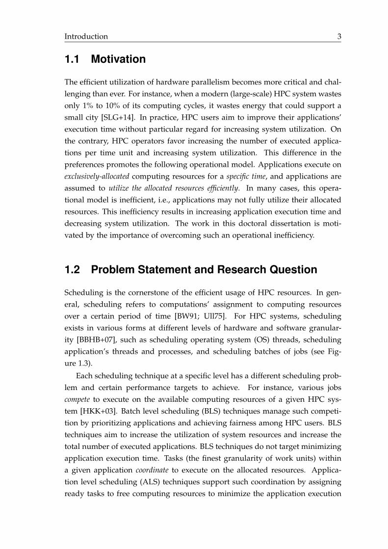
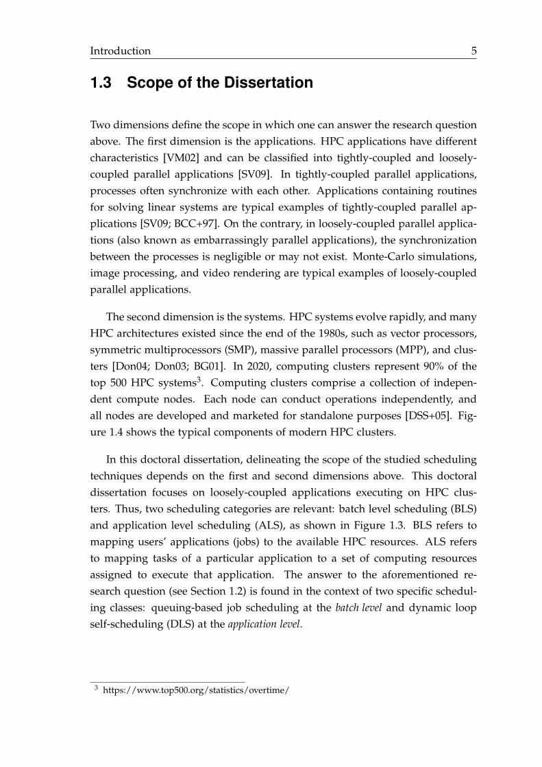
1.3 Clustering of multilevel scheduling (MLS) into batch level schedul-ing (BLS) and application level scheduling (ALS) . . . . . . . . . . . . 4
1.4 System components of modern HPC clusters. . . . . . . . . . . . . . . . 6
1.5 The four research stages of the work presented in this doctoral dis-sertation . . . . . . . . . . . . . . . . . . . . . . . . . . . . . . . . . . . . 7
2.1 Chunk sizes generated by different DLS techniques. . . . . . . . . . . . 23
3.1 The execution workflow of the SimGrid simulator and the proposedextensions to support BLS. . . . . . . . . . . . . . . . . . . . . . . . . . . 34
3.2 The execution workflow of the GridSim simulator and the proposedextensions to support ALS. . . . . . . . . . . . . . . . . . . . . . . . . . 35
3.3 Performance of the SimGrid and GridSim simulators in terms of sim-ulation wall clock time for the selected ALS techniques. . . . . . . . . . 37
3.4 Performance of the SimGrid and GridSim simulators in terms of sim-ulation wall clock time for the selected BLS techniques. . . . . . . . . . 38
3.5 Bridging simulator instances. . . . . . . . . . . . . . . . . . . . . . . . . 39
3.6 The two-level scheduling simulator. . . . . . . . . . . . . . . . . . . . . 42
3.7 The system makespan of the W 241 workload for several BLS-ALS com-
binations. . . . . . . . . . . . . . . . . . . . . . . . . . . . . . . . . . . . . 45
3.8 The system makespan of the W 242 workload for several BLS-ALS com-
binations. . . . . . . . . . . . . . . . . . . . . . . . . . . . . . . . . . . . . 45
3.9 Effect of changing the task variation factor Υ considering the W 241
workload. . . . . . . . . . . . . . . . . . . . . . . . . . . . . . . . . . . . . 46
3.10 Effect of changing the task variation factor Υ considering the W 242
workload. . . . . . . . . . . . . . . . . . . . . . . . . . . . . . . . . . . . . 46
3.11 The ratio between system makespan w/ and w/o task variation Υconsidering the W 24
1 workload. . . . . . . . . . . . . . . . . . . . . . . . 47
3.12 The ratio between system makespan w/ and w/o task variation Υconsidering the W 24
2 workload. . . . . . . . . . . . . . . . . . . . . . . . 47
xiv List of Figures
3.13 Snapshot of the Vampir visualization tool showing the generatedOTF2 trace of the proposed two-level scheduling simulator. . . . . . . 48
3.14 The simulation wall clock time of the two-level scheduling simulator. 49
4.1 Variants of the master-worker execution model, as reported in theliterature. . . . . . . . . . . . . . . . . . . . . . . . . . . . . . . . . . . . . 53
4.2 Schematic execution of the proposed distributed chunk calculationapproach (DCA). . . . . . . . . . . . . . . . . . . . . . . . . . . . . . . . 58
4.3 The proposed DCA. . . . . . . . . . . . . . . . . . . . . . . . . . . . . . . 59
4.4 Performance of the proposed DCA vs. the existing master-workerbased approach for PSIA. . . . . . . . . . . . . . . . . . . . . . . . . . . 65
4.5 Performance of the proposed DCA vs. the existing master-workerbased approach for Mandelbrot. . . . . . . . . . . . . . . . . . . . . . . 66
5.1 The proposed hierarchical distributed chunk calculation approach(HDCA). . . . . . . . . . . . . . . . . . . . . . . . . . . . . . . . . . . . . 72
5.2 The undesired synchronization with the MPI+OpenMP implementa-tion approach. . . . . . . . . . . . . . . . . . . . . . . . . . . . . . . . . . 73
5.3 An ideal execution scenario at the shared-memory level. . . . . . . . . 73
5.4 Parallel execution time of the main loop using STATIC at the firstlevel of scheduling (inter-node scheduling). . . . . . . . . . . . . . . . . 75
5.5 Parallel execution time of the main loop using GSS at the first level ofscheduling (inter-node scheduling). . . . . . . . . . . . . . . . . . . . . 77
5.6 Parallel execution time of the main loop using TSS at the first level ofscheduling (inter-node scheduling). . . . . . . . . . . . . . . . . . . . . 78
5.7 Parallel execution time of the main loop using FAC2 at the first levelof scheduling (inter-node scheduling). . . . . . . . . . . . . . . . . . . . 79
6.1 Proposed resourceful coordination approach (RCA). . . . . . . . . . . . 82
6.2 ESP job arrival scheme. . . . . . . . . . . . . . . . . . . . . . . . . . . . . 87
6.3 Load imbalance profile of the jobs within the ESP-PSIA and ESP-Mandelbrotworkloads. . . . . . . . . . . . . . . . . . . . . . . . . . . . . . . . . . . . 88
6.4 System utilization for the ESP-PSIA workload. . . . . . . . . . . . . . . 90
6.5 System utilization for the ESP-Mandelbrot workload. . . . . . . . . . . 90
6.6 Visualization (obtained using Vampir) of the execution trace of theESP-Mandelbrot workload. . . . . . . . . . . . . . . . . . . . . . . . . . 92
6.7 Visualization (obtained using Vampir) of the execution trace of theESP-PSIA workload. . . . . . . . . . . . . . . . . . . . . . . . . . . . . . 93
List of Figures xv
7.1 The MLS prototype. . . . . . . . . . . . . . . . . . . . . . . . . . . . . . . 957.2 The centralized chunk calculation approach (CCA) in LB4MPI. . . . . 977.3 The distribution chunk calculation approach (DCA) in LB4MPI. . . . . 977.4 Parallel application execution time of PSIA in the three slowdown
scenarios. . . . . . . . . . . . . . . . . . . . . . . . . . . . . . . . . . . . . 1017.5 Parallel application execution time of Mandelbrot in the three slow-
down scenarios. . . . . . . . . . . . . . . . . . . . . . . . . . . . . . . . . 1027.6 The main components of Slurm. . . . . . . . . . . . . . . . . . . . . . . 1047.7 System makespan of the ESP (Mandelbrot) with different application
level scheduling techniques. Slurm is configured to use FCFS for BLS. 108

List of Tables
2.1 Notation used to describe the selected loop scheduling techniques . . 16
3.1 Notation of the proposed connection layer for the two-level schedul-ing simulation approach . . . . . . . . . . . . . . . . . . . . . . . . . . . 41
3.2 Characteristics of the workloads selected from the parallel workloadarchive (PWA) . . . . . . . . . . . . . . . . . . . . . . . . . . . . . . . . . 44
4.1 Execution parameters of PSIA and Mandelbrot selected to evaluatethe proposed DCA . . . . . . . . . . . . . . . . . . . . . . . . . . . . . . 61
4.2 Ratios between the KNL and Xeon core count . . . . . . . . . . . . . . 62
5.1 Mapping between the DLS techniques and the OpenMP scheduleclause options . . . . . . . . . . . . . . . . . . . . . . . . . . . . . . . . . 74
6.1 Characteristics of the two implemented versions of the ESP systembenchmark: ESP-PSIA and ESP-Mandelbrot. . . . . . . . . . . . . . . . 86
7.1 Software and hardware components of the MLS cluster . . . . . . . . . 107


List of Tables xix

1Introduction
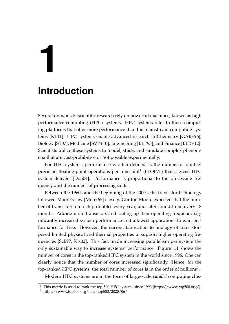
Several domains of scientific research rely on powerful machines, known as highperformance computing (HPC) systems. HPC systems refer to those comput-ing platforms that offer more performance than the mainstream computing sys-tems [KT11]. HPC systems enable advanced research in Chemistry [GAB+96],Biology [ST07], Medicine [SVP+10], Engineering [BLP95], and Finance [BLR+12].Scientists utilize these systems to model, study, and simulate complex phenom-ena that are cost-prohibitive or not possible experimentally.
For HPC systems, performance is often defined as the number of double-precision floating-point operations per time unit1 (FLOP/s) that a given HPCsystem delivers [Don04]. Performance is proportional to the processing fre-quency and the number of processing units.
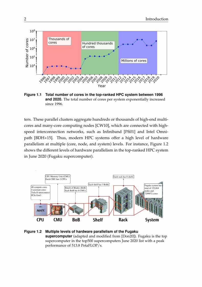
Between the 1960s and the beginning of the 2000s, the transistor technologyfollowed Moore’s law [Moo+65] closely. Gordon Moore expected that the num-ber of transistors on a chip doubles every year, and later found to be every 18months. Adding more transistors and scaling up their operating frequency sig-nificantly increased system performance and allowed applications to gain per-formance for free. However, the current fabrication technology of transistorsposed limited physical and thermal properties to support higher operating fre-quencies [Sch97; Kis02]. This fact made increasing parallelism per system theonly sustainable way to increase systems’ performance. Figure 1.1 shows thenumber of cores in the top-ranked HPC system in the world since 1996. One canclearly notice that the number of cores increased significantly. Hence, for thetop-ranked HPC systems, the total number of cores is in the order of millions2.
Modern HPC systems are in the form of large-scale parallel computing clus-
1 This metric is used to rank the top 500 HPC systems since 1993 (https://www.top500.org/)2 https://www.top500.org/lists/top500/2020/06/
2 Introduction
199619
9719
9819
9920
0020
0120
0220
0320
0420
0520
0620
0720
0820
0920
1020
1120
1220
1320
1420
1520
1620
1720
1820
1920
20
Year
104
105
106
107
108Nu
mbe
r of c
ores Thousands of
cores Hundred thousands of cores
Millions of cores
Figure 1.1 Total number of cores in the top-ranked HPC system between 1996and 2020. The total number of cores per system exponentially increasedsince 1996.
ters. These parallel clusters aggregate hundreds or thousands of high-end multi-cores and many-core computing nodes [CW10], which are connected with high-speed interconnection networks, such as Infiniband [Pfi01] and Intel Omni-path [BDH+15]. Thus, modern HPC systems offer a high level of hardwareparallelism at multiple (core, node, and system) levels. For instance, Figure 1.2shows the different levels of hardware parallelism in the top-ranked HPC systemin June 2020 (Fugaku supercomputer).
48 compute cores4 assistant cores Tofu-D interconnectPCIe Gen3
CPU Memory Unit (CMU)Each CMU has 2 CPUs
Bunch of Blades (BoB)Each BoB has 8 CMUs
Each shelf has 3 BoBs
Each rack has 8 shelfs
Fugaku system has total of 152,064 nodes and 7299072 cores
Figure 1.2 Multiple levels of hardware parallelism of the Fugakusupercomputer (adapted and modified from [Don20]). Fugaku is the topsupercomputer in the top500 supercomputers June 2020 list with a peakperformance of 513.8 PetaFLOP/s.
Introduction 3
1.1 Motivation
The efficient utilization of hardware parallelism becomes more critical and chal-lenging than ever. For instance, when a modern (large-scale) HPC system wastesonly 1% to 10% of its computing cycles, it wastes energy that could support asmall city [SLG+14]. In practice, HPC users aim to improve their applications’execution time without particular regard for increasing system utilization. Onthe contrary, HPC operators favor increasing the number of executed applica-tions per time unit and increasing system utilization. This difference in thepreferences promotes the following operational model. Applications execute onexclusively-allocated computing resources for a specific time, and applications areassumed to utilize the allocated resources efficiently. In many cases, this opera-tional model is inefficient, i.e., applications may not fully utilize their allocatedresources. This inefficiency results in increasing application execution time anddecreasing system utilization. The work in this doctoral dissertation is moti-vated by the importance of overcoming such an operational inefficiency.
1.2 Problem Statement and Research Question
Scheduling is the cornerstone of the efficient usage of HPC resources. In gen-eral, scheduling refers to computations’ assignment to computing resourcesover a certain period of time [BW91; Ull75]. For HPC systems, schedulingexists in various forms at different levels of hardware and software granular-ity [BBHB+07], such as scheduling operating system (OS) threads, schedulingapplication’s threads and processes, and scheduling batches of jobs (see Fig-ure 1.3).
Each scheduling technique at a specific level has a different scheduling prob-lem and certain performance targets to achieve. For instance, various jobscompete to execute on the available computing resources of a given HPC sys-tem [HKK+03]. Batch level scheduling (BLS) techniques manage such competi-tion by prioritizing applications and achieving fairness among HPC users. BLStechniques aim to increase the utilization of system resources and increase thetotal number of executed applications. BLS techniques do not target minimizingapplication execution time. Tasks (the finest granularity of work units) withina given application coordinate to execute on the allocated resources. Applica-tion level scheduling (ALS) techniques support such coordination by assigningready tasks to free computing resources to minimize the application execution
4 Introduction
time [BBHB+07]. ALS techniques aim to decrease application execution time.ALS techniques do not target increasing system utilization. Batch and applica-tion scheduling techniques work separately without coordination.
In 1993, the absence of coordination between job, task, and thread schedulersat the operating system (OS) and application levels was identified and solved forsystems of that time (multiprocessor computers with shared memory) [Nag93].However, for modern HPC systems, non-coordinated scheduling decisions ofbatch and application schedulers is still relevant and remains an open researchproblem [BBHB+07; DGGL+18].
Multilevel scheduling (MLS) refers to exchanging scheduling information be-tween scheduling levels, such as batch, application, and OS level. MLS helps inrefining scheduling decisions at a certain level based on the available informa-tion about the current scheduling workload at other levels. We formulate thefollowing research question to address the problem of coordination absence be-tween schedulers at different scheduling levels: How can MLS exploit the multiplelevels of hardware parallelism of a modern HPC system to enhance scientific applica-tions’ performance and increase utilization of HPC resources?
OSthread
Application
Local batch
Globalbatch
CoreNode
Cluster
Grid
Leve
ls of
sof
twar
e pa
ralle
lism
Levels of hardware parallelism
Global job
Thread
OS level scheduling
Batch level scheduling
Processlevel scheduling
Multilevel scheduling
Local job
Process/Thread
Appl
icatio
n le
vel s
ched
ulin
g
Threadlevel scheduling
Grid level scheduling
Figure 1.3 Clustering of multilevel scheduling (MLS) into batch levelscheduling (BLS) and application level scheduling (ALS)
Introduction 5
1.3 Scope of the Dissertation
Two dimensions define the scope in which one can answer the research questionabove. The first dimension is the applications. HPC applications have differentcharacteristics [VM02] and can be classified into tightly-coupled and loosely-coupled parallel applications [SV09]. In tightly-coupled parallel applications,processes often synchronize with each other. Applications containing routinesfor solving linear systems are typical examples of tightly-coupled parallel ap-plications [SV09; BCC+97]. On the contrary, in loosely-coupled parallel applica-tions (also known as embarrassingly parallel applications), the synchronizationbetween the processes is negligible or may not exist. Monte-Carlo simulations,image processing, and video rendering are typical examples of loosely-coupledparallel applications.
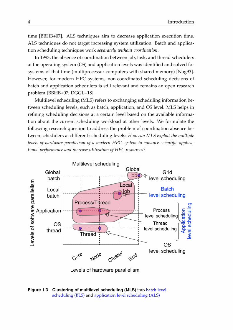
The second dimension is the systems. HPC systems evolve rapidly, and manyHPC architectures existed since the end of the 1980s, such as vector processors,symmetric multiprocessors (SMP), massive parallel processors (MPP), and clus-ters [Don04; Don03; BG01]. In 2020, computing clusters represent 90% of thetop 500 HPC systems3. Computing clusters comprise a collection of indepen-dent compute nodes. Each node can conduct operations independently, andall nodes are developed and marketed for standalone purposes [DSS+05]. Fig-ure 1.4 shows the typical components of modern HPC clusters.
In this doctoral dissertation, delineating the scope of the studied schedulingtechniques depends on the first and second dimensions above. This doctoraldissertation focuses on loosely-coupled applications executing on HPC clus-ters. Thus, two scheduling categories are relevant: batch level scheduling (BLS)and application level scheduling (ALS), as shown in Figure 1.3. BLS refers tomapping users’ applications (jobs) to the available HPC resources. ALS refersto mapping tasks of a particular application to a set of computing resourcesassigned to execute that application. The answer to the aforementioned re-search question (see Section 1.2) is found in the context of two specific schedul-ing classes: queuing-based job scheduling at the batch level and dynamic loopself-scheduling (DLS) at the application level.
3 https://www.top500.org/statistics/overtime/
6 Introduction
Compute node 1
Compute node n
Compute node 2
Clus
ter i
nter
conn
ectio
n ne
twor
k Compute node 3
Resource and job management system (RJMS) Main controller daemon
Operating system
Compute resources Network interface
RMJS
ut
ilitie
s
Head nodeHPC users
Compute resources
RMJS
da
emon
Network interface
User applications
Parallel runtime systems
Operating system
RMJS
da
emon
Network interface
User applications
Parallel runtime systems
Operating system
RMJS
da
emon User applications
Parallel runtime systems
Operating system
Compute resources
RMJS
da
emon
Network interface
User applications
Parallel runtime systems
Operating system
Compute resources
Compute resources Network interface
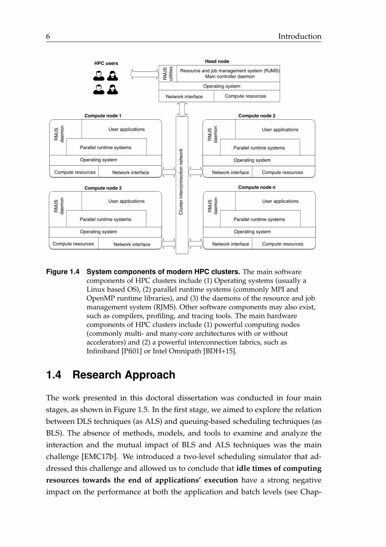
Figure 1.4 System components of modern HPC clusters. The main softwarecomponents of HPC clusters include (1) Operating systems (usually aLinux based OS), (2) parallel runtime systems (commonly MPI andOpenMP runtime libraries), and (3) the daemons of the resource and jobmanagement system (RJMS). Other software components may also exist,such as compilers, profiling, and tracing tools. The main hardwarecomponents of HPC clusters include (1) powerful computing nodes(commonly multi- and many-core architectures with or withoutaccelerators) and (2) a powerful interconnection fabrics, such asInfiniband [Pfi01] or Intel Omnipath [BDH+15].
1.4 Research Approach
The work presented in this doctoral dissertation was conducted in four mainstages, as shown in Figure 1.5. In the first stage, we aimed to explore the relationbetween DLS techniques (as ALS) and queuing-based scheduling techniques (asBLS). The absence of methods, models, and tools to examine and analyze theinteraction and the mutual impact of BLS and ALS techniques was the mainchallenge [EMC17b]. We introduced a two-level scheduling simulator that ad-dressed this challenge and allowed us to conclude that idle times of computingresources towards the end of applications’ execution have a strong negativeimpact on the performance at both the application and batch levels (see Chap-
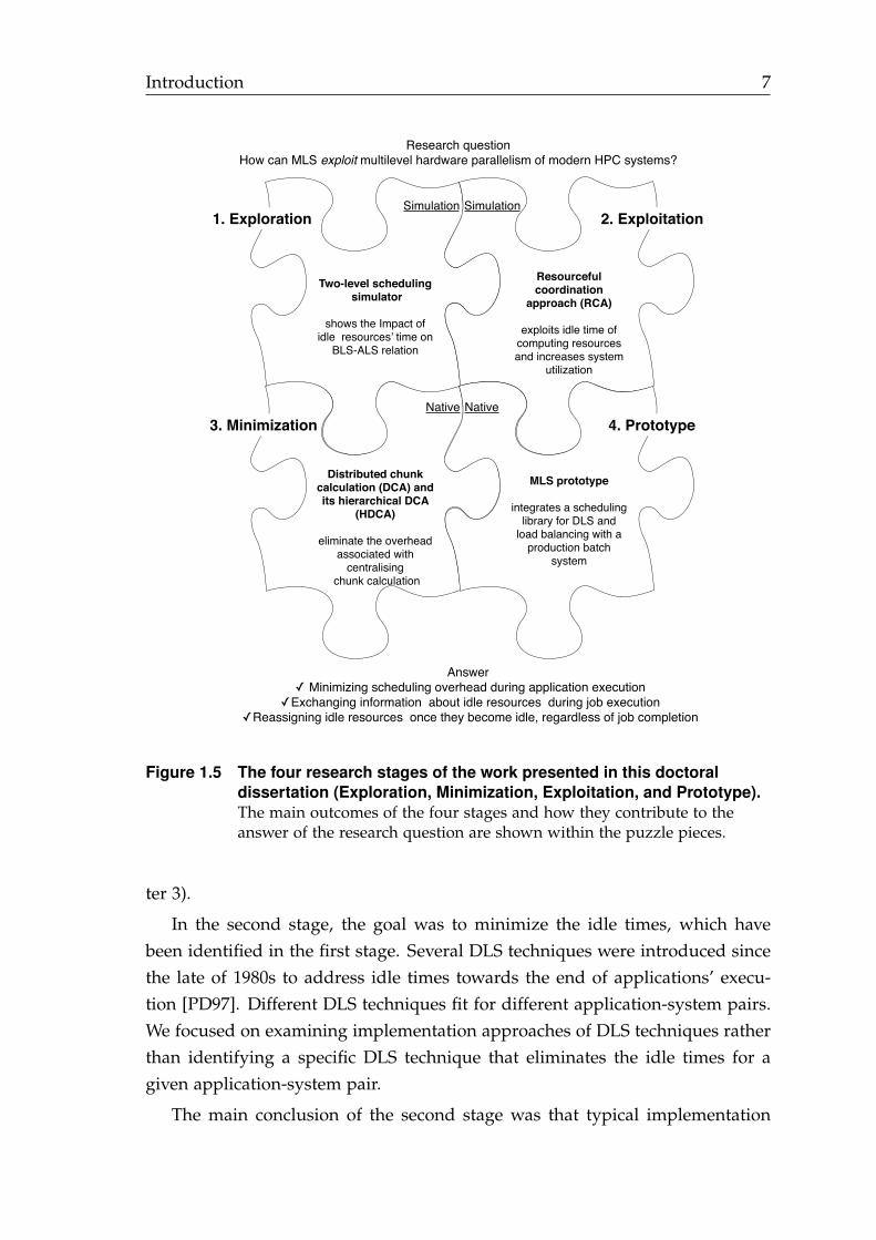
Introduction 7
Two-level scheduling simulator
shows the Impact of idle resources’ time on
BLS-ALS relation
Distributed chunk calculation (DCA) and its hierarchical DCA
(HDCA)
eliminate the overhead associated with
centralising chunk calculation
Resourceful coordination
approach (RCA)
exploits idle time of computing resources and increases system
utilization
MLS prototype
integrates a scheduling library for DLS and
load balancing with a production batch
system
1. Exploration
3. Minimization
2. Exploitation
4. Prototype
Research questionHow can MLS exploit multilevel hardware parallelism of modern HPC systems?
Answer ✓ Minimizing scheduling overhead during application execution
✓Exchanging information about idle resources during job execution✓Reassigning idle resources once they become idle, regardless of job completion
Simulation Simulation
Native Native
Figure 1.5 The four research stages of the work presented in this doctoraldissertation (Exploration, Minimization, Exploitation, and Prototype).The main outcomes of the four stages and how they contribute to theanswer of the research question are shown within the puzzle pieces.
ter 3).
In the second stage, the goal was to minimize the idle times, which havebeen identified in the first stage. Several DLS techniques were introduced sincethe late of 1980s to address idle times towards the end of applications’ execu-tion [PD97]. Different DLS techniques fit for different application-system pairs.We focused on examining implementation approaches of DLS techniques ratherthan identifying a specific DLS technique that eliminates the idle times for agiven application-system pair.
The main conclusion of the second stage was that typical implementation
8 Introduction
approaches of DLS techniques introduce additional overhead, which contributesto idle times of computing resources. We introduced a distributed chunk cal-culation approach (DCA) and its hierarchical version (HDCA) to eliminate theadditional overhead. DCA avoids the overhead of centralizing chunk calculationand assignment at a single computing resource (see Chapters 4 and 5).
Achieving a perfectly balanced execution of a given parallel loop is an ex-tremely challenging task [BVD03]. DLS techniques allow PEs to have nearlyequal finishing times by assigning chunks of independent loop iteration to freeprocessing elements (PEs). However, achieving the exact same finishing time ispractically infeasible [MC20].
In the third stage, the goal was to exploit idle time when PEs do not have thesame finishing times. We introduced a resourceful coordination approach (RCA)that allows one application to share its idle computing resources with other ap-plications through the batch system. RCA solves the problem discussed in Sec-tion 1.2 by enabling coordination between the application and batch schedulers(see Chapter 6). The coordination, in this case, refers to sharing informationabout idle computing resources (by application schedulers) and decisions of re-assigning these computing resources to other pending applications (by the batchscheduler).
In the last stage, we provided a scheduling prototype that combines all ourproposed scheduling approaches. For instance, DCA was implemented in anMPI-based scheduling library, called LB4MPI [MEC+20; MC20]. Also, RCA wasimplemented in a production batch scheduler, called Slurm [YJG03]. Notifica-tion messages were sent from LB4MPI to Slurm once a resource becomes idle,and consequently, Slurm was able to reassign that resource to other pendingjobs. By combining DCA and RCA, the scheduling prototype presented in Chap-ter 7 represents a production scheduler that employs MLS to exploit modern HPCsystems efficiently.
1.4.1 Evaluation Methodology
The work presented in this doctoral dissertation was evaluated via simulationand native experiments. Both evaluation methods are used to assess perfor-mance of scheduling techniques. Simulation experiments allow exploration ofvarious scenarios with minimum cost. For instance, executing large workloadson an HPC system requires the full reservation of that system and can takeseveral days to complete. In the exploration stage (see Figure 1.5), we evalu-ated twelve combinations of four ALS and three BLS techniques. The cost of
Introduction 9
executing such experiments as native experiments is not affordable, i.e., one ex-periment takes 13 days (see Chapter 3). Similarly, for the exploitation stage (seeFigure 1.5), the proposed RCA at the batch level was evaluated via simulation(see Chapter 6).
The main advantage of native experiments is the realistic and trustworthyresults [BFM+06]. Native experiments let scheduling techniques experience allvariability of a real execution environment, which can be abstracted, simplified,or ignored in simulation. In the minimization stage (see Figure 1.5), we exploitedsuch an advantage and evaluated the proposed DCA and HDCA via nativeexperiments (see Chapters 4 and 5). We also used native experiments to assessthe potential of the MLS prototype (see Chapter 7).
1.5 Contributions
Throughout the work in this doctoral dissertation, the following contributionshave been made to solve the research problem discussed in Section 1.2.
1. Two-level scheduling simulation approach: A novel simulation approachthat bridges two different scheduling simulators by exchanging schedulinginformation among the bridged scheduling simulators [EMC17b]. The pro-posed approach is exemplified with a two-level simulator that bridges twowell-known simulators: SimGrid [EMC16; MEC+20] for ALS and Grid-Sim [KMR07; KR10] for BLS. The newly introduced two-level schedulingsimulator stores simulation events produced by both simulators. It alsointegrates all simulation events into a single file in the OTF2 [EWG+11]format. This format is compatible with trace visualization tools, such asVampir [KBD+08].
The significance of this contribution is: enabling the simulations of HPCworkloads at fine (tasks within applications) and coarse (jobs within aworkload) scales, i.e., it allowed us to explore the relation between ALS andBLS techniques by examining various combinations of these techniques(see Chapter 3). The two-level simulation approach contributes to thesolution of the MLS problem by identifying idle times of computing re-sources as a root-cause of the performance degradation at that batch andapplication levels. Thus, our research focused on coordinating schedul-ing decisions between batch and application schedulers to minimize andexploit these idle times.
10 Introduction
2. Distributed chunk calculation approach (DCA): The proposed DCA en-sures that every PE can calculate its chunk independently, i.e., the calcu-lated chunk size at any PE does not rely on any information about thechunk size calculated at other PEs. The proposed DCA requires all DLStechniques to have a straightforward chunk calculation formula. A straight-forward chunk calculation formula requires only constants and input parame-ters, and it does not require prior information about previously calculatedchunk sizes. We provide the mathematical transformation needed to en-sure that all the chunk calculation formulas of the selected DLS techniquesare straightforward formulas (see Chapter 4).
The significance of this contribution is replacing the common master-worker execution model that is used mainly to implement DLS techniqueson distributed-memory systems. The proposed DCA overcomes certain well-known limitations of the master-worker model. The DCA contributesto the solution of the MLS problem by providing a generic executionmodel that eliminates the overhead of centralizing chunk calculation andassignment on a single computing resource. Thus, it reduces idle times ofcomputing resources.
3. Hierarchical distributed chunk calculation approach (HDCA): DLS tech-niques assume a centralized work queue. All PEs obtain chunks of iterationto execute from that work queue. Similar to the hierarchical master-workerexecution model for DLS [WYL+12], HDCA maintains local work queuesfor each group of PEs that share the same physical memory address space.The local work queues are always filled with new work from the globalcentral queue. The novelty of the proposed HDCA is that the responsi-bility of maintaining local work queues is shared among all PEs withinthe same group. In the hierarchical master-worker execution model, suchresponsibility is assigned only to specific PEs (local masters).
The significance of this contribution is enabling efficient and scalable im-plementations of hierarchical DLS techniques. The HDCA contributes tothe solution of the MLS problem by eliminating another source of over-head, and consequently, minimizing idle times of computing resources.
4. Resourceful coordination approach (RCA): RCA enables the cooperationbetween the currently independent batch and application level schedulers.RCA enables application schedulers to share their allocated but idle com-puting resources with other applications through the batch system. RCA
Introduction 11
avoids resource shrinking operations and associated performance penaltiestypical of dynamic resource and job management systems.
The significance of this contribution is that the proposed RCA increasesthe entire system utilization and decreases the system makespan whenthe applications suffer from a severe load imbalance. For long-executingHPC applications, the proposed RCA showed that exploiting idle times ofcomputing resources (which are in the order of a few seconds) can signif-icantly improve the entire system utilization. To the best of our knowl-edge and prior to this work, it was commonly accepted that the shortidle times of computing resources can only be exploited by Big Data work-loads [MGG+17]. RCA highlights the potential of exploring such idle timesfor HPC workloads as well (see Chapter 6). The RCA contributes to thesolution of the MLS problem by providing a mechanism to coordinatescheduling decisions of batch and application schedulers to exploit idletimes of computing resources [EC21].
5. The multilevel scheduling (MLS) prototype: is a software solution thatimplements the MLS concepts and addresses the absence of coordination be-tween schedulers at different levels by employing:
a) The proposed DCA to minimize application execution times.
b) The proposed RCA to increase system utilization.
The MLS prototype connects the job scheduler of Slurm [YJG03] with theLB4MPI scheduling library [MEC+20; MC20].
The MLS prototype contributes to the solution of the MLS problem by gath-ering, implementing, and applying all the contributions of this doctoral disser-tation in a production HPC environment, i.e., the MLS prototype confirms theusefulness of the MLS solution in real HPC production systems.
1.6 Outline of the Thesis
The remainder of this doctoral dissertation is organized as follows. In Chapter 2,the two selected scheduling classes of queuing-based scheduling (at the batchlevel) and dynamic loop scheduling (at the application level) are introduced.Chapter 2 also focuses on the performance goals for each scheduling class andvarious performance metrics used in the literature to assess the techniques ofboth scheduling classes.

12 Introduction
Chapter 3 describes the first contribution of this doctoral work, which is thetwo-level scheduling simulation approach. The need and advantages of bridgingtwo different simulators [MEC+20; KMR07] are discussed. The limited benefitof existing HPC workload traces for the two-level simulation is also discussed.The strategy of using a task variation factor to overcome such a limitation is pre-sented. The chapter ends with a performance evaluation of twelve combinationsof four DLS techniques and three queuing-based scheduling techniques.
The distributed chunk calculation approach [EC19a] and its hierarchical ver-sion [EC19b] are described in Chapters 4 and 5, respectively. Both chapters startby discussing the limitations of existing DLS implementations that motivate theproposed DCA and HDCA. Both chapters end with a performance evaluationof the proposed approach in different scenarios.
The resourceful coordination approach (RCA) is described in Chapter 6 withdetails on how it is integrated into the Slurm simulator [SIJ+17]. Chapter 6 alsodescribes how the effective system performance (ESP) benchmark [WOK+00b]is used to assess the proposed RCA in simulation.
In Chapter 7, the MLS prototype is introduced. The detailed modificationsand extensions made to LB4MPI and Slurm are presented and discussed. Thechapter ends with an evaluation and discussion regarding the performance ofthe MLS prototype. Chapter 8 presents the conclusion of this thesis and anoutlook on future research.
1.7 Publications
Following is a list of the publications that are directly and tightly-connected tothe contributions of this doctoral dissertation.
[EC21] A. Eleliemy and F. M. Ciorba. A Resourceful coordination Approach forMultilevel Scheduling. In Proceedings of the International Conference onHigh Performance Computing & Simulation (HPCS 2021), virtual event,2021.
[EC20] A. Eleliemy and F. M. Ciorba. A Distributed Chunk Calculation Approachfor Self-scheduling of Parallel Applications on Distributed-memory Sys-tems. Journal of Computational Science (JOCS), 2021.
[EC19b] A. Eleliemy and F. M. Ciorba. Hierarchical Dynamic Loop Schedulingon Distributed-Memory Systems Using an MPI+MPI Approach. In Pro-
Introduction 13
ceedings of the 20th IEEE International Workshop on Parallel and Dis-tributed Scientific and Engineering Computing (PDSEC 2019) of the 33rdIEEE International Parallel and Distributed Processing Symposium Work-shops and PhD Forum (IPDPSW 2019), Rio de Janeiro, Brazil, 2019.
[EC19a] A. Eleliemy and F. M. Ciorba. Dynamic Loop Scheduling Using MPI Passive-Target Remote Memory Access. In Proceedings of the 27th EuromicroInternational Conference on Parallel, Distributed and Networked-based(PDP 2019), Pavia, Italy, 2019.
[EMC17b] A. Eleliemy, A. Mohammed, and F. M. Ciorba. Exploring the RelationBetween Two Levels of Scheduling Using a Novel Simulation Approach.In the proceedings of the 16th International Symposium on Parallel andDistributed Computing (ISPDC 2017), Innsbruck, Austria, 2017.
[EMC17a] A. Eleliemy, A. Mohammed, and F. M. Ciorba. Efficient Generation of Par-allel Spin-images Using Dynamic Loop Scheduling. In Proceedings of the8th International Workshop on Multicore and Multithreaded Architecturesand Algorithms (M2A2 2017) in conjunction with the 19th IEEE Interna-tional Conference for High Performance Computing and Communications(HPCC 2017), Bangkok, Thailand, 2017.
During my doctoral work, I have also contributed to other research efforts.I consider the following publications, which I have co-authored, are indirectlyrelated to my doctoral work. I could make benefit of them to my work in simu-lation, performance analysis, and scheduling in general. These publications areas follows:
[MEC+20] A. Mohammed, A. Eleliemy, F. M. Ciorba, F. Kasielke, and I. Banicescu. AnApproach for Realistically Simulating the Performance of Scientific Ap-plications on High Performance Computing Systems. Journal of FutureGeneration Computer Systems (FGCS), 111:617–633, 2020.
[MEC+18] A. Mohammed, A. Eleliemy, and F. M. Ciorba. Experimental Verifica-tion and Analysis of Dynamic Loop Scheduling in Scientific Applications.In Proceedings of the 17th International Symposium on Parallel and Dis-tributed Computing (ISPDC 2018), Geneva, 2018.
[MEC18] A. Mohammed, A. Eleliemy, and F. M. Ciorba. Performance Reproductionand Prediction of Selected Dynamic Loop Scheduling Experiments. In Pro-

14 Introduction
ceedings of the International Conference on High Performance Computing& Simulation (HPCS 2018), Orléans, France, 2018.
[EFM+16] A. Eleliemy, M. Fayze, R. Mehmood, I. Katib, and N. Aljohani Loadbal-ancing on Parallel Heterogeneous Architectures: Spin-image Algorithm onCPU and MIC. In Proceedings of the 9th Eurosim Congress on Modelingand Simulation (EUROSIM 2016), Oulu, Finland, 2016.
2Scheduling in HPC Systems
Scheduling can be defined as mapping units of work to computing resourcesover a specific period of time [BW91; Ull75]. Scheduling exists in various formsat different levels of hardware parallelism of HPC systems (core, node, andsystem). Hence, each level requires and employs techniques for appropriatescheduling of the computational work at the respective level [BBHB+07].
This chapter focuses on dynamic loop self-scheduling (DLS) at the appli-cation level and queuing-based job scheduling at the batch level. The mostwell-known techniques from each class are presented in this chapter. Moreover,the performance metrics that can be used to assess those scheduling techniquesare reviewed.
2.1 Application Level Scheduling (ALS)
An application refers to a computer program that executes on one or multiplecomputing resources to accomplish a specific job. Computer applications oftenconsist of multiple tasks representing the finest granularity of computations. Atask cannot be divided into a finer granularity and cannot execute on multiplecomputing resources simultaneously. Application level scheduling (ALS) refersto mapping tasks of a particular application to a set of computing resourcesassigned to execute that application.
The majority of applications that execute on HPC systems are scientific appli-cations that often contain large computationally-intensive parallel loops. Theseloops represent the prime source of parallelism, and their execution dominatesthe entire application performance [FTY+90]. Scientific applications, such ascomputational field simulation on unstructured grids, N-body, and Monte-Carlo
16 Scheduling in HPC Systems
simulations, are typical examples in which loop scheduling is crucial for the per-formance [BVD03; BFH95]. In the context of loop scheduling, a loop iterationis the finest granularity that can be mapped to a computing resource. Hence, aloop iteration can refer to a task.
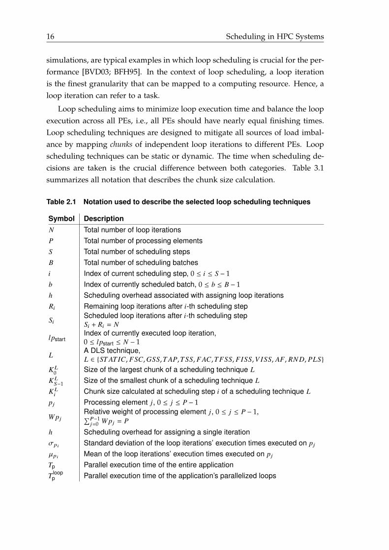
Loop scheduling aims to minimize loop execution time and balance the loopexecution across all PEs, i.e., all PEs should have nearly equal finishing times.Loop scheduling techniques are designed to mitigate all sources of load imbal-ance by mapping chunks of independent loop iterations to different PEs. Loopscheduling techniques can be static or dynamic. The time when scheduling de-cisions are taken is the crucial difference between both categories. Table 3.1summarizes all notation that describes the chunk size calculation.
Table 2.1 Notation used to describe the selected loop scheduling techniques
Symbol DescriptionN Total number of loop iterationsP Total number of processing elementsS Total number of scheduling stepsB Total number of scheduling batchesi Index of current scheduling step, 0 ≤ i ≤ S − 1b Index of currently scheduled batch, 0 ≤ b ≤ B − 1h Scheduling overhead associated with assigning loop iterationsRi Remaining loop iterations after i-th scheduling step
SiScheduled loop iterations after i-th scheduling stepSi + Ri = N
lpstartIndex of currently executed loop iteration,0 ≤ lpstart ≤ N − 1
LA DLS technique,L ∈ {ST AT IC, FSC, GSS, T AP, T SS, F AC, T FSS, FISS, V ISS, AF, RN D, PLS}
KL0 Size of the largest chunk of a scheduling technique L
KLS−1 Size of the smallest chunk of a scheduling technique L
KLi Chunk size calculated at scheduling step i of a scheduling technique L
pj Processing element j, 0 ≤ j ≤ P − 1
W pjRelative weight of processing element j, 0 ≤ j ≤ P − 1,∑P−1
j=0 W pj = P
h Scheduling overhead for assigning a single iterationσpi Standard deviation of the loop iterations’ execution times executed on pj
µpi Mean of the loop iterations’ execution times executed on pj
Tp Parallel execution time of the entire applicationT loop
p Parallel execution time of the application’s parallelized loops
Scheduling in HPC Systems 17
2.1.1 Static Loop Scheduling (SLS)
Static loop scheduling (SLS) takes scheduling decisions before application ex-ecution. The chunk sizes and their assignment are known before the execu-tion. Block, cyclic and block-cyclic represent various examples of SLS tech-niques [LTS+93]. Block [LTS+93], also known as STATIC, is a straightforwardtechnique that divides the loop into P chunks of equal size, as shown in Eq. 2.1.Each chunk is assigned to a corresponding PE, i.e., the ith chunk is assigned tothe ith PE.
K ST AT ICi =
NP
(2.1)
Cyclic and block-cyclic also assign the same amount of loop iterations to eachPE, i.e., each PE gets a total number of iterations that is equal to N
P . However,in cyclic, the loop iterations are distributed one by one in a cyclic fashion. Incontrast, block-cyclic scheduling distributes blocks of loop iterations in a cyclicfashion. Because SLS techniques take scheduling decisions before applicationexecution, they incur the minimum scheduling overhead, and they have lesscapability to balance the execution of loops in highly irregular execution envi-ronments.
2.1.2 Dynamic Loop Self-scheduling (DLS)
Dynamic loop scheduling-self (DLS) techniques take scheduling decisions dur-ing application execution. Compared to SLS, DLS techniques incur significantscheduling overhead, but they are more capable of balancing the loop execu-tion than SLS techniques, especially in highly irregular execution environments.DLS techniques have been used in different applications, such as N-body sim-ulation [BFH95], computational fluid dynamics [BVD03], solar map genera-tion [BWA16], spin-image generation [EMC17a], and heat conduction [BV02].Furthermore, DLS techniques can be divided into non-adaptive and adaptivetechniques.
2.1.2.1 Non-adaptive DLS
The non-adaptive techniques utilize the information that is obtained before theapplication execution. The non-adaptive techniques include self-scheduling (SS) [PPC86],fixed size self-scheduling (FSC) [KW85], guided self-scheduling (GSS) [PK87],taper (TAP) [Luc92], trapezoid self-scheduling (TSS) [TN93], factoring (FAC) [FHSF92],weighted factoring (WF) [FHSU+96] trapezoid factoring self-scheduling (TFSS) [CAB+01],
18 Scheduling in HPC Systems
fixed increase self-scheduling (FISS) [PD97], variable increase self-scheduling (VISS) [PD97],random (RND) [CIB18], and performance-based loop scheduling (PLS) [SYT07].
SS [PPC86] is a dynamic self-scheduling technique where the chunk sizeis always one iteration, as shown in Eq. 2.2. SS has the highest schedulingoverhead because it has the maximum number of chunks, i.e., the total numberof chunks is N . However, SS can achieve a highly load-balanced execution inhighly irregular execution environments.
K SSi = 1 (2.2)
As a middle point between STATIC and SS, FSC assumes an optimal chunksize that achieves a balanced execution of loop iterations with the smallest over-head. To calculate such an optimal chunk size, FSC considers the variabilityin iterations’ execution time and the scheduling overhead of assigning loop it-erations to be known before applications’ execution. Eq. 2.3 shows how FSCcalculates the optimal chunk size.
KFSCi =
√2 · N · h
σ · P ·√
log P(2.3)
GSS [PK87] is also a compromise between the highest load balancing that canbe achieved using SS and the lowest scheduling overhead incurred by STATIC.Unlike FSC, GSS assigns decreasing chunk sizes to balance loop executionsamong all PEs. At every scheduling step, GSS assigns a chunk that is equalto the number of remaining loop iterations divided by the total number of PEs,as shown in Eq. 2.4.
KGSSi =
Ri
P, where
Ri = N −i−1∑j=0
kGSSj
(2.4)
TAP [Luc92] is based on a probabilistic analysis that represents a generalcase of GSS. It considers the average of loop iterations’ execution time µ and thestandard deviation σ to achieve a higher load balance than GSS. Eq. 2.5 showshow TAP tunes the GSS chunk size based on µ and σ.
KT APi = KGSS
i +v2α
2− vα ·
√2 · KGSS
i +v2α
4, where
vα =α · σ
µ
(2.5)
Scheduling in HPC Systems 19
TSS [TN93] assigns decreasing chunk sizes similar to GSS. However, TSSuses a linear function to decrement chunk sizes. This linearity results in lowscheduling overhead in each scheduling step compared to GSS. Eq. 2.6 showsthe linear function of TSS.
KT SSi = KT SS
i−1 −
⎢⎢⎢⎢⎢⎣
KT SS0 − KT SS
S−1
S − 1
⎥⎥⎥⎥⎥⎦, where
S =⎡⎢⎢⎢⎢⎢
2 · NKT SS
0 + KT SSS−1
⎤⎥⎥⎥⎥⎥KT SS
0 =
⌈N
2 · P
⌉, KT SS
S−1 = 1
(2.6)
FAC [FHSF92] schedules the loop iterations in batches of equally-sized chunks.FAC evolved from comprehensive probabilistic analyses, and it assumes priorknowledge about µ and σ. Another practical implementation of FAC denoted,FAC2, assigns half of the remaining loop iterations for every batch, as shown inEq. 2.7. The initial chunk size of FAC2 is half of the initial chunk size of GSS.If more time-consuming loop iterations are at the beginning of the loop, FAC2may better balance their execution than GSS.
KF AC2i =
⎧⎪⎨⎪⎩
⌈Ri
2·P
⌉, if i mod P = 0
KF AC2i−1 , otherwise.
, where
Ri = N −i−1∑j=0
kF AC2j
(2.7)
WF [FHSU+96] is based on FAC. However, each PE executes variably-sizedchunks of a given batch according to its relative weights. The processor weights,Wpj , are determined prior to applications’ execution and do not change duringthe execution. WF2 is the practical implementation of WF that is based on FAC2,as shown in Eq 2.8.
KW F2i = KF AC2
i ·Wpj (2.8)
TFSS [CAB+01] combines certain characteristics of TSS [TN93] and FAC [FHSF92].Similar to FAC, TFSS schedules loop iterations in batches of equally-sized chunks.However, it does not follow the analysis of FAC, i.e., every batch is not half ofthe remaining number of iterations. Batches in TFSS decrease linearly, similar tochunk sizes in TSS. As shown in Eq. 2.9, TFSS calculates the chunk size as thesum of the next P chunks that would have been computed by the TSS dividedby P.
KTFSSi =
⎧⎪⎪⎨⎪⎪⎩
∑i+P−1j=i KTSS
j
P if i mod P = 0KTFSS
i−1 , otherwise.(2.9)
20 Scheduling in HPC Systems
GSS [PK87], TAP [Luc92], TSS [TN93], FAC [FHSF92], and TFSS[CAB+01]employ a decreasing chunk size pattern. This pattern introduces additionalscheduling overhead due to the small chunk sizes towards the end of the loopexecution. On distributed-memory systems, the additional scheduling overheadis more substantial than on shared-memory systems. FISS [PD97] is the firstscheduling technique devised explicitly for distributed-memory systems. FISSfollows an increasing chunk size pattern calculated as in Eq. 2.10. FISS dependson an initial value B defined by the user (suggested to be equal to the FAC’stotal number of batches).
KFISSi = KFISS
i−1 + ⌈2 · N · (1 − B
2+B )P · B · (B − 1)
⌉, where
KFISS0 =
N(2 + B) · P
(2.10)
VISS [PD97] follows an increasing pattern of chunk sizes. Unlike FISS, VISSrelaxes the requirement of defining an initial value B. VISS works similarly toFAC2, but instead of decreasing the chunk size, VISS increments the chunk sizeby a factor of two per scheduling step. Eq. 2.11 shows the chunk calculation ofVISS.
KV ISSi =
⎧⎪⎪⎨⎪⎪⎩
KV ISSi−1 +
KV ISSi−12 if i mod P = 0
KV ISSi−1 , otherwise.
, where
KV ISS0 = KFISS
0
(2.11)
RND [CIB18] is a DLS technique that utilizes a uniform random distributionto arbitrarily choose a chunk size between specific lower and upper bounds.The lower and the upper bounds were suggested to be N
100·P and N2·P , respec-
tively [CIB18]. In the current work, we suggest a lower and an upper boundas 1 and N
P , respectively. These bounds make RND have an equal probabilityof selecting any chunk size between the chunk size of STATIC and the chunksize of SS, which are the two extremes of DLS techniques in terms of schedulingoverhead and load balancing. Eq. 2.12 represents the integer range of the RNDchunk sizes.
K RN Di ∈ [1, N/P] (2.12)
PLS [SYT07] combines the advantages of SLS and DLS. It divides the loopinto two parts. The first loop part is scheduled statically. In contrast, the secondpart is scheduled dynamically using GSS. The static workload ratio (SWR) isused to determine the amount of the iterations to be statically scheduled. SWR iscalculated as the ratio between minimum and maximum iteration execution time
Scheduling in HPC Systems 21
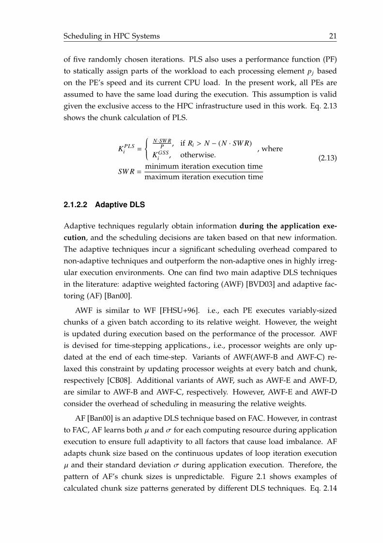
of five randomly chosen iterations. PLS also uses a performance function (PF)to statically assign parts of the workload to each processing element p j basedon the PE’s speed and its current CPU load. In the present work, all PEs areassumed to have the same load during the execution. This assumption is validgiven the exclusive access to the HPC infrastructure used in this work. Eq. 2.13shows the chunk calculation of PLS.
K PLSi =
⎧⎪⎨⎪⎩
N ·SW RP , if Ri > N − (N · SW R)
KGSSi , otherwise.
, where
SW R =minimum iteration execution timemaximum iteration execution time
(2.13)
2.1.2.2 Adaptive DLS
Adaptive techniques regularly obtain information during the application exe-cution, and the scheduling decisions are taken based on that new information.The adaptive techniques incur a significant scheduling overhead compared tonon-adaptive techniques and outperform the non-adaptive ones in highly irreg-ular execution environments. One can find two main adaptive DLS techniquesin the literature: adaptive weighted factoring (AWF) [BVD03] and adaptive fac-toring (AF) [Ban00].
AWF is similar to WF [FHSU+96]. i.e., each PE executes variably-sizedchunks of a given batch according to its relative weight. However, the weightis updated during execution based on the performance of the processor. AWFis devised for time-stepping applications., i.e., processor weights are only up-dated at the end of each time-step. Variants of AWF(AWF-B and AWF-C) re-laxed this constraint by updating processor weights at every batch and chunk,respectively [CB08]. Additional variants of AWF, such as AWF-E and AWF-D,are similar to AWF-B and AWF-C, respectively. However, AWF-E and AWF-Dconsider the overhead of scheduling in measuring the relative weights.
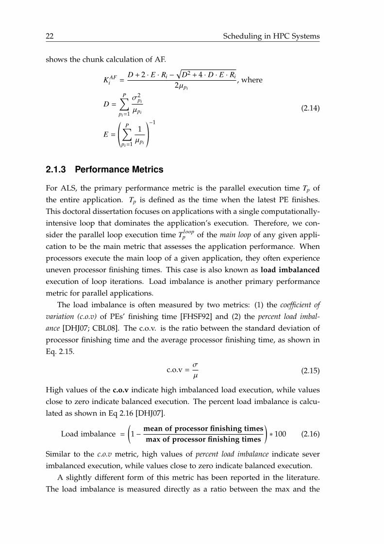
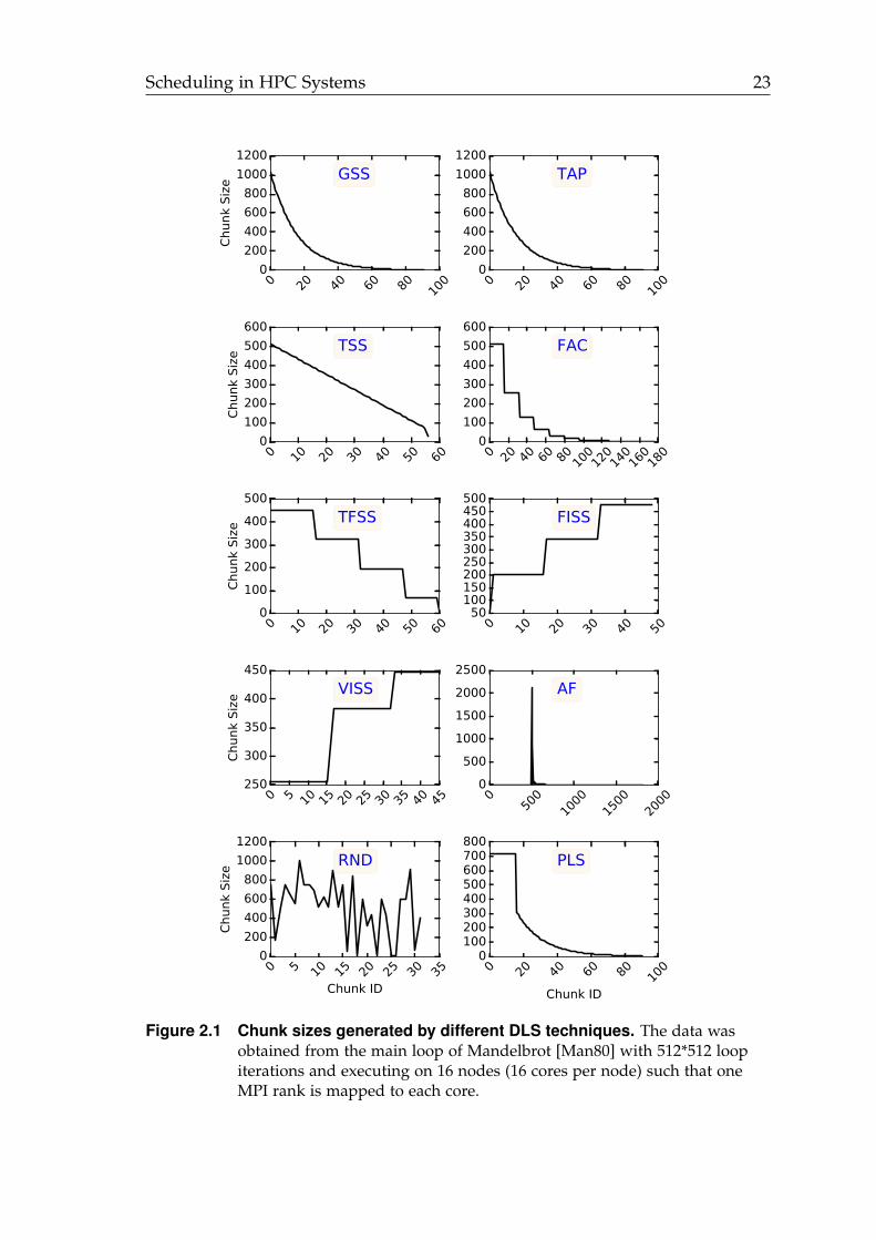
AF [Ban00] is an adaptive DLS technique based on FAC. However, in contrastto FAC, AF learns both µ and σ for each computing resource during applicationexecution to ensure full adaptivity to all factors that cause load imbalance. AFadapts chunk size based on the continuous updates of loop iteration executionµ and their standard deviation σ during application execution. Therefore, thepattern of AF’s chunk sizes is unpredictable. Figure 2.1 shows examples ofcalculated chunk size patterns generated by different DLS techniques. Eq. 2.14
22 Scheduling in HPC Systems
shows the chunk calculation of AF.
K AFi =
D + 2 · E · Ri −√
D2 + 4 · D · E · Ri
2µpi, where
D =P∑
pi=1
σ2pi
µpi
E = *.,
P∑pi=1
1µpi
+/-
−1
(2.14)
2.1.3 Performance Metrics
For ALS, the primary performance metric is the parallel execution time Tp ofthe entire application. Tp is defined as the time when the latest PE finishes.This doctoral dissertation focuses on applications with a single computationally-intensive loop that dominates the application’s execution. Therefore, we con-sider the parallel loop execution time T loop
p of the main loop of any given appli-cation to be the main metric that assesses the application performance. Whenprocessors execute the main loop of a given application, they often experienceuneven processor finishing times. This case is also known as load imbalancedexecution of loop iterations. Load imbalance is another primary performancemetric for parallel applications.
The load imbalance is often measured by two metrics: (1) the coefficient ofvariation (c.o.v) of PEs’ finishing time [FHSF92] and (2) the percent load imbal-ance [DHJ07; CBL08]. The c.o.v. is the ratio between the standard deviation ofprocessor finishing time and the average processor finishing time, as shown inEq. 2.15.
c.o.v =σ
µ(2.15)
High values of the c.o.v indicate high imbalanced load execution, while valuesclose to zero indicate balanced execution. The percent load imbalance is calcu-lated as shown in Eq 2.16 [DHJ07].
Load imbalance =(1 −
mean of processor finishing timesmax of processor finishing times
)∗ 100 (2.16)
Similar to the c.o.v metric, high values of percent load imbalance indicate severimbalanced execution, while values close to zero indicate balanced execution.
A slightly different form of this metric has been reported in the literature.The load imbalance is measured directly as a ratio between the max and the
Scheduling in HPC Systems 23
0 20 40 60 80 100
0
200
400
600
800
1000
1200
Chunk
Siz
e
GSS
0 20 40 60 80 100
0
200
400
600
800
1000
1200
TAP
0 10 20 30 40 50 600
100
200
300
400
500
600
Chunk
Siz
e
TSS
0 20 40 60 80 100
120
140
160
180
0
100
200
300
400
500
600
FAC
0 10 20 30 40 50 600
100
200
300
400
500
Chunk
Siz
e
TFSS
0 10 20 30 40 5050
100150200250300350400450500
FISS
0 5 10 15 20 25 30 35 40 45250
300
350
400
450
Chunk
Siz
e
VISS
050
010
0015
0020
000
500
1000
1500
2000
2500
AF
0 5 10 15 20 25 30 35
Chunk ID
0
200
400
600
800
1000
1200
Chunk
Siz
e
RND
0 20 40 60 80 100
Chunk ID
0100200300400500600700800
PLS
Figure 2.1 Chunk sizes generated by different DLS techniques. The data wasobtained from the main loop of Mandelbrot [Man80] with 512*512 loopiterations and executing on 16 nodes (16 cores per node) such that oneMPI rank is mapped to each core.
24 Scheduling in HPC Systems
mean of processor finishing times [PGW+17]. In that case, the metric is called(max/mean), and when the value of max/mean is close to one, the load executionis balanced.
2.2 Batch Level Scheduling (BLS)
Users of HPC systems execute their applications as batch jobs. A batch job repre-sents a request of specific computing resources for a limited time to execute particularapplication binaries [FBP15][Rod17, page. 6]. Batch level scheduling (BLS) refersto mapping users’ jobs to the available HPC resources. Resource and job man-agement systems (RJMSs), also known as a batch system, are critical componentsof HPC systems. RJMSs are responsible for BLS, job life cycle management, re-source management, and job execution [RBA+18]. One may consider RJMSs asoperating systems for HPC systems [GH12]. There are two different classifi-cations of RJMSs: (1) static vs. dynamic [FR96; PIR+14] and (2) planning vs.queuing [HKK+03] systems.
2.2.1 Static vs. Dynamic Batch Systems
Static RJMSs are systems that provide static resource allocation to jobs, i.e., theresource allocation cannot be changed once the job starts. In contrast, dynamicRJMS change resource allocation during job execution. The concept of staticand dynamic resource allocation is tightly coupled with the four types of batchjobs [FRS+97]: (1) Rigid jobs which are the most common type of job foundin HPC systems. A Rigid job is a request for a specific number of computingresources that are necessary to execute the application binaries. (2) Moldablejobs which are similar to rigid jobs. However, RJMSs have the flexibility tochange the number of the requested computing resources before the applicationstarts. Once applications start, the batch system cannot change their resourceallocation. (3) Malleable jobs which refer to the preferred jobs for any batchsystem, i.e., the resource allocation of a malleable job can be changed by thebatch system at any time. (4) Evolving jobs which refer to jobs that request anadditional computing resource from the batch system during their execution.Static RJMSs support the first two types of jobs (rigid and moldable jobs), whiledynamic RJMS support the other two types (malleable and evolving jobs). Mostbatch systems support only static allocation [PIR+14]. A few production batchsystems, such as Slurm [YJG03], only provide certain sort of support for dynamic
Scheduling in HPC Systems 25
allocation. In Slurm, resource expansion is done by allowing a running job tosubmit a new job with a dependency indicator and merging the allocations.Slurm requires all the resources assigned dynamically for the job to be releasedtogether [Pra16, page. 17].
2.2.2 Planning vs. Queuing Batch Systems
Planning batch systems, such as the computing center software (CCS) [KR01],create a schedule with start times of all requests. The execution estimate of sub-mitted jobs is a mandatory information for planning systems. With every in-coming request or request that ends before it was estimated, planning systemscompute a new schedule. The earliest suitable gap (ESG) and local search (LS)based optimization routine are examples of planning-based scheduling [KR11].
Queuing batch systems, such as Slurm [YJG03] and PBS [Hen95], hold sev-eral queues with different configurations (limits on requested resources or onrequested time). Users of queuing batch systems submit their queues to spe-cific queues. Batch queuing systems assign free resources to the waiting jobs inthe queues. They apply various queuing-based job scheduling techniques, alsoknown as priority scheduling techniques, to select a job for execution. First comefirst serve (FCFS), earliest deadline first (EDF), and shortest job first (SJF) are ex-amples of queuing-based scheduling [KMR07; ABS+11]. Most of the existingbatch systems are queuing systems [HKK+03].
2.2.3 Queuing-based Job Scheduling
In FCFS, the batch scheduler sorts the queue based on the job submission time.Jobs with the earliest submission time become at the head of the queue. InEDF, the batch scheduler sorts the queue based on the job due date (deadline).The job with the soonest deadline becomes the head of the queue. In SJF, thebatch scheduler sorts the queue based on the job expected execution time. Thejob with the minimum expected execution becomes the head of the queue. Thebatch system does not start the job at the head of the queue unless all its requiredresources are free. In many cases, the available resources may be sufficient tostart other jobs rather than the job at the head of the queue. These cases motivatethe backfilling (BF) scheduling technique [FW98].
BF is a supporting scheduling technique that allows scheduling of jobs outof order from a given queue as long as those jobs do not delay the start time ofjobs placed at the beginning of the queue [FW98]. BF helps to execute small jobs
26 Scheduling in HPC Systems
(which request a small number of computing resources) when insufficient avail-able computing resources are needed to execute the highest priority jobs. BF isclassified into conservative BF and EASY BF. Conservative BF only chooses forexecution the small jobs (with short execution time and requests a few comput-ing resources) that their execution will not cause a delay to any of the waitingjobs, including the job at the head of the queue. In contrast, EASY BF onlyensures that the waiting job at the queue’s head will not be delayed when thesmall jobs are executed.
Most of the production batch systems, such as Slurm [YJG03], LSF [IBM16],and PBS [Hen95], allow user to define custom priority scheduling. For instance,the batch system may be configured to higher priorities to the jobs submittedby a certain user or group of users. Also, many fairness policies may be ap-plied. For instance, a fair-share scheduling technique prioritizes queued jobssuch that an under-serviced user is scheduled first. The goal of such a fair-sharescheduling technique is maintaining the same average job waiting time acrossall users.
2.2.4 Other Job Scheduling Techniques
Gang scheduling [FR95; FJ97] allows all jobs to execute concurrently on the sameset of computing resources using a time-slicing mechanism. Each job receivesthe request computing resources for a time slice (quantum). The scheduler thenswitches the context to allow another job to execute on the same computing re-sources set for another quantum. Gang scheduling relies on stopping one ormore low-priority jobs to let high-priority jobs execute (also known as Preemp-tion).
Bin packing [CGJ83] scheduling selects groups of jobs to launch simultane-ously on one or a set of computing resources. The packed jobs are selectedto maximize the utilization of the allocated resources. Gang and bin packingscheduling are not commonly used. FCFS and EASY BF are the most commonjob scheduling techniques for real productions HPC system [GGR+15].
2.2.5 Performance Metrics
System makespan (Tbatch) is measured as the total execution time of the entirebatch. System makespan is shown in Eq. 2.17 where Ti is the time when the firstjob starts and Tj is the time when the last job in the batch completes.
Tbatch = Tj −Ti (2.17)
Scheduling in HPC Systems 27
Short system makespan indicates better system performance. However, onemay not be able to use it to assess the HPC systems’ scheduling techniques. Inproduction, HPC systems continuously accept new jobs as users submit them.Hence, there is no fixed workload with a specific end. System utilization (SU)is a crucial metric that one may use to assess batch systems’ performance. Itrefers to the percentage of the resources used over a time frame [FTK14; Xha10].Eq. 6.1 shows the calculation of SU where Tk is the time that a computing re-source k spent executing jobs, P is the total number the computing resources.SU ranges from 0% to 100%.
SU =∑P−1
k=0 Tk
P ∗Tbatch∗ 100% (2.18)
Higher values of system utilization indicate better system performance.System throughput measures the number of jobs completed per unit time.
Batch schedulers should maintain high values of system throughput. Hence,they indicate better system availability.
Average job waiting time is the average time that jobs spend waiting forresources before execution. Eq. 2.19 shows the job average waiting time, whereJ start
i and J submiti are the start and the submit time of job Ji, respectively, and N
is the total number of jobs.
Average job waiting time =∑N−1
i=0 J starti − J submit
i
N(2.19)
A lower average waiting time indicates better system performance.
2.3 Related State of the Art in Scheduling
The dynamic resource ownership management (DROM) is a recent research ef-fort that allows RMJS to address efficient resource usage challenge [DGGL+18].DROM provides effortless malleability for RMJS that requires no change in ap-plications’ source codes. DROM exploits the finest level of parallelism to sup-port application malleability, i.e., changing the number of the threads assignedto a computing resource to create a new room for other applications on thesame computing resource. One may use DROM with load balancing librariessimilar to LeWI [GCL09] (LeWI is a runtime library that uses standard mech-anisms, such as OMPT [Ope20] to monitor application execution.). LeWI canenhance application performance and increase resource utilization of individ-ual computing nodes. A holistic dynamic scheduling policy, called slowdown
28 Scheduling in HPC Systems
driven (SD-policy) [DJC19] was proposed based on DROM. The SD-policy ap-plies backfilling by selecting small jobs to share nodes with other running jobs.The SD-policy depends on DROM to achieve efficient node-sharing.
DROM and the LeWI library are similar to the MLS prototype because theytarget the same challenge of efficient resource usage. However, DROM relieson the malleability of the parallel runtime systems used by the applications,such as OpenMP or OmpSs to change the number of active threads withoutaffecting running applications. This may not be suitable for applications thatdo not use a malleable parallel runtime system, such as the message-passinginterface (MPI). In contrast, the MLS prototype does not require applicationsto be malleable. Furthermore, it enables coordination between the schedulingof different applications via batch systems. For instance, waiting or runningapplications (need more computing resources) may communicate their needs tothe RJMS, which requests other MPI-based applications to stop scheduling anyworkload on the required computing resources certain period. In this scenario,the schedulers of different applications coordinate with each other through theRJMS. When an application scheduler decides not to schedule any workload ona particular resource, the process can be entirely suspended by the operatingsystem, and other applications can use their computing resource.
A notable research effort implemented an elastic execution framework forMPI applications [CMHG+16]. The framework introduced certain extensionsto the MPI standard and to Slurm [YJG03]. These extensions permit a dynamicchange of the number of processes of a given application in a way that addressesseveral challenges of the original dynamic process support of the MPI standard.The elastic framework requires application scientists to use the new MPI func-tions to support application malleability. Such a requirement could be a draw-back or a limitation of the elastic MPI framework. A large-scale study that ex-amined more than one hundred MPI applications showed that most of the MPIapplications only use MPI 1.0 features [LMM+19]. For instance, non-blockingcollectives and neighborhood collectives are MPI 3.0 features and found to be inless than 1% of the examined applications. The cost of rewriting working codescan be one of the reasons behind that fact.
This elastic MPI framework has the same goals as the MLS prototype. How-ever, the MLS prototype shifts the responsibility of releasing or requesting com-puting resource to the application scheduler rather than the application codeitself. Moreover, in the MLS prototype, allowing one application to share idlecomputing resources with other applications does not require shrinking opera-

Scheduling in HPC Systems 29
tions at that application’s side, which keeps overhead low.

3Two-level Scheduling Simulator
Studying mutual impacts of various scheduling levels requires conducting sev-eral exploratory experiments. These experiments involve trials of many combi-nations of scheduling techniques. In many cases, the associated cost of such anexploratory study is unaffordable. Simulation approaches mitigate such costsand enable the study of complex systems [STL+15; MEC+20].
This chapter introduces a novel scheduling simulation approach that bridgestwo different scheduling simulators by exchanging scheduling information amongthem [EMC17b]. Based on our approach, we have developed and assessed atwo-level scheduling simulator that employs well-known simulation toolkits:SimGrid [CGL+14] and GridSim [BM02]. Our two-level scheduling simula-tor enables the simulations of HPC workloads at fine (tasks within applica-tions) and coarse (jobs within a workload) scales. We visualize the simulationevents collected from both simulators by converting them into an OTF2-basedtrace [EWG+11] that is compatible with trace visualization tools, such as Vam-pir [KBD+08].
3.1 Application and Batch Level SchedulingSimulations
SimGrid [CGL+14] is a widely used simulation toolkit for ALS [HCB17; SBS+13;BSC+12]. SimGrid supports the development of parallel and distributed appli-cations in heterogeneous and homogeneous environments. Recent releases ofSimGrid have three different interfaces: MetaSimGrid (MSG), SimDag (SD), andSimulated MPI (SMPI). MSG simulates applications as a group of concurrentprocesses. SD simulates directed acyclic graphs (DAGs). SMPI executes un-
32 Two-level Scheduling Simulator
modified applications written using the message passing interface (MPI) in asimulation mode. SimGrid also has a new interface called S4U that is plannedto replace the other three interfaces in the future.
GridSim [BM02] is another simulation toolkit that is widely used for BLS.GridSim facilitates simulation of grids, clusters, and single processing elements.It offers support for a broad range of heterogeneous resources, including sharedand distributed memory architectures. GridSim is built on top of a reliablediscrete event simulation library called SimJava [How98]. The GridSim toolkitis fully implemented in Java, which promotes its portability and extensibility.
We use a SimGrid-based scheduling simulator that is based on the SD in-terface [EMC16] for the ALS simulations. This specific SimGrid simulator hasthe advantage of being experimentally verified and capable of achieving a closeagreement to native executions in various scenarios [MEC+18; MEC+20]. For theBLS simulations herein, we use a GridSim-based scheduling simulator, calledAlea [KMR07; KR10; KSS19]. This GridSim-based simulator has the advantageof offering a wide range of implemented and verified BLS techniques, such asFCFS, EDF, SJF, and BF [FW98].
The SimGrid [CGL+14] and GridSim [BM02] simulation toolkits are prefer-ably used (not restricted) to support ALS and BLS, respectively. Certain re-search efforts (described below) studied extensions of one of these two simula-tion toolkits to support the simulation of other scheduling levels.
3.1.0.1 ALS Simulation Based on a BLS Simulation Toolkit
Alea [KMR07] is a GridSim-based simulator. A remarkable research effort [SBC+11]extended Alea to support ALS. Four scheduling techniques were implementedin the extension, including SS [PPC86], FSC [KW85], GSS [PK87], and FAC [FHSF92].The extension carried over all the Alea’s advantages to the ALS domain, suchas application tasks being expressed in standard workload format (SWF) [Fei20]and the effect of system failures being examined with different ALS techniques.However, the extension supported ALS in such a way that it can no longer sup-port BLS.
3.1.0.2 BLS Simulation Based on an ALS Simulation Toolkit
Simbatch [Can08] is a SimGrid-based simulator. Simbatch uses the MSG inter-face of SimGrid to support simulations and the development of BLS techniques.Simbatch’s uniqueness comes from the fact that it swaps the focus of SimGridfrom the ALS perspective to the BLS perspective. However, Simbatch supports
Two-level Scheduling Simulator 33
two basic batch scheduling techniques FCFS [ABS+11] and BF [FW98]. Further-more, Simbatch cannot support ALS.
Both SimGrid [CGL+14] and GridSim [BM02] have been used to support ALSand BLS simulation. However, none of these simulators was used to supportholistic simulation. In the context of this doctoral dissertation, holistic simula-tion refers to ALS and BLS’s simultaneous simulation. This simulation is essen-tial to understand the BLS-ALS relation and exploit the multilevel parallelismaspect of contemporary HPC systems.
Two critical questions arise: (1) Which simulator should we extend to sup-port BLS-ALS simulations? And (2) How does the selected simulator supportBLS-ALS simulations? The answer of the first question is not straightforward,because the selected simulator has to be the most suitable one for both BLSand ALS. An important question raises regarding how suitability is defined andmeasured. Both the SimGrid [EMC16] and GridSim [BM02] are event-basedsimulators, i.e., both will have the same simulation results when one simulatesthe same events as the other. Therefore, we judge the “suitability” with thefollowing two evaluation criteria: (1) the simulation wall clock and (2) the cus-tomization effort. The simulation wall clock is the time one simulator takes toconduct the simulation and produce the simulation results. The customizationeffort is the development effort associated with extending a simulator to supportALS or BLS simulation. The customization effort is proportional to the numberof lines of code.
Figures 3.1 and 3.2 show the proposed extensions (in the GridSim [BM02]and SimGrid [CGL+14] simulators) that enable simulation of ALS and BLS. Theextensions in both simulators rely on a flag called the ALS switch. If a usersets the ALS switch to true, the simulation is considered as an ALS simula-tion; otherwise, it is considered as a BLS simulation. One may wonder aboutthe reason for having such a flag, i.e., can we extend each of the two simula-tors by implementing scheduling techniques at both levels directly? Of course,both simulators require implementing the scheduling techniques at both lev-els. For instance, we have implemented ALS techniques, such as FSC [KW85],GSS [PK87], and FAC [FHSF92], for the GridSim simulator. Also, we have imple-mented BLS techniques, such as FCFS, SJF, and EDF, for the SimGrid simulator.However, the implementation of these scheduling techniques in both simulatorsis insufficient to enable simulation of ALS and BLS. The entire simulation flowin both cases is not the same.
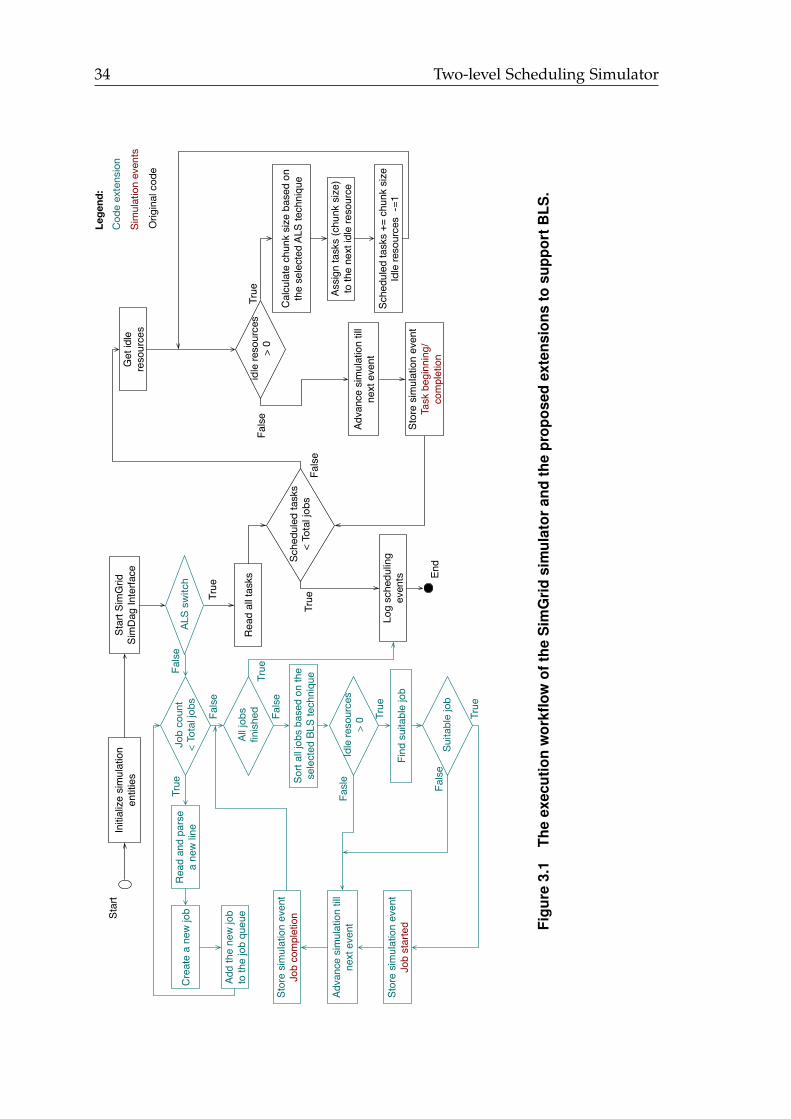
34 Two-level Scheduling Simulator
Initi
aliz
e si
mul
atio
n en
titie
sSt
art S
imG
rid
Sim
Dag
Inte
rface
ALS
switc
hFa
lse
True
Job
coun
t<
Tota
l job
sR
ead
and
pars
e a
new
line
Tr
ue
True
Add
the
new
job
to th
e jo
b qu
eue
Cre
ate
a ne
w jo
b
All j
obs
finis
hed Fa
lse
Sort
all j
obs
base
d on
the
sele
cted
BLS
tech
niqu
e
Idle
reso
urce
s >
0 True
Fals
e
Log
sche
dulin
g ev
ents
Fi
nd s
uita
ble
job
Suita
ble
job
Adva
nce
sim
ulat
ion
till
next
eve
ntFa
sle
Stor
e si
mul
atio
n ev
ent
Job
com
plet
ion
Stor
e si
mul
atio
n ev
ent
Job
star
ted
True
Rea
d al
l tas
ks
Sche
dule
d ta
sks
< To
tal j
obs
Get
idle
re
sour
ces
Fals
eTr
ue
idle
reso
urce
s >
0Tr
ue
Cal
cula
te c
hunk
siz
e ba
sed
on
the
sele
cted
ALS
tech
niqu
e
Assi
gn ta
sks
(chu
nk s
ize)
to th
e ne
xt id
le re
sour
ceAd
vanc
e si
mul
atio
n til
lne
xt e
vent
Fals
e
Sche
dule
d ta
sks
+= c
hunk
siz
eId
le re
sour
ces
-=1
Stor
e si
mul
atio
n ev
ent
Task
beg
inni
ng/
com
plet
ion
Cod
e ex
tens
ion
Lege
nd:
Sim
ulat
ion
even
tsO
rigin
al c
ode
Fals
e
Star
t
End
Figu
re3.
1Th
eex
ecut
ion
wor
kflow
ofth
eS
imG
rid
sim
ulat
oran
dth
epr
opos
edex
tens
ions
tosu
ppor
tBLS
.
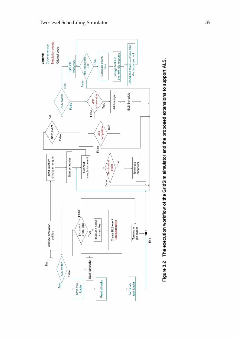
Two-level Scheduling Simulator 35
Initi
aliz
e si
mul
atio
n en
titie
sSt
art G
ridSi
m
sim
ulat
ion
engi
ne
Star
t tas
k lo
ader
Star
t sch
edul
er
ALS
switc
h
Star
t job
load
er
True
Fals
e
Rea
d al
l tas
ks
Term
inat
e ta
sk lo
ader
job
coun
t<
tota
l job
s
Rea
d an
d pa
rse
a ne
w li
ne
True
Fals
e
Term
inat
e jo
b lo
ader
Cre
ate
BLS
even
t Jo
b su
bmis
sion
New
_eve
ntTr
ue
ALS
switc
hFa
lse Jo
b co
mpl
etio
n
True
Get
nex
t si
mul
atio
n ev
ent
True
Term
inat
ion
even
t
Fals
e
True
Term
inat
e sc
hedu
ler
Job
subm
issi
on
Fals
e
True
Add
new
job
BLS
Sche
dule
Fals
e
Cod
e ex
tens
ion
Lege
nd:
Sim
ulat
ion
even
tsO
rigin
al c
ode
Fals
e
Fals
e
Get
idle
re
sour
ces
idle
_res
ourc
es
> 0 Tr
ue
Cal
cula
te c
hunk
si
ze
Assi
gn ta
sks
toth
e ne
xt id
le re
sour
ce
Sche
dule
d ta
sks
+= c
hunk
siz
eId
le re
sour
ces
-=1
Star
t
End
Figu
re3.
2Th
eex
ecut
ion
wor
kflow
ofth
eG
ridS
imsi
mul
ator
and
the
prop
osed
exte
nsio
nsto
supp
ortA
LS.
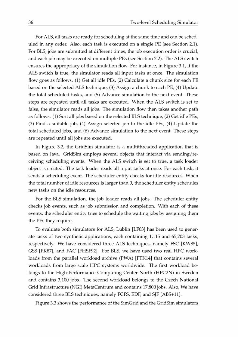
36 Two-level Scheduling Simulator
For ALS, all tasks are ready for scheduling at the same time and can be sched-uled in any order. Also, each task is executed on a single PE (see Section 2.1).For BLS, jobs are submitted at different times, the job execution order is crucial,and each job may be executed on multiple PEs (see Section 2.2). The ALS switchensures the appropriacy of the simulation flow. For instance, in Figure 3.1, if theALS switch is true, the simulator reads all input tasks at once. The simulationflow goes as follows. (1) Get all idle PEs, (2) Calculate a chunk size for each PEbased on the selected ALS technique, (3) Assign a chunk to each PE, (4) Updatethe total scheduled tasks, and (5) Advance simulation to the next event. Thesesteps are repeated until all tasks are executed. When the ALS switch is set tofalse, the simulator reads all jobs. The simulation flow then takes another pathas follows. (1) Sort all jobs based on the selected BLS technique, (2) Get idle PEs,(3) Find a suitable job, (4) Assign selected job to the idle PEs, (4) Update thetotal scheduled jobs, and (6) Advance simulation to the next event. These stepsare repeated until all jobs are executed.
In Figure 3.2, the GridSim simulator is a multithreaded application that isbased on Java. GridSim employs several objects that interact via sending/re-ceiving scheduling events. When the ALS switch is set to true, a task loaderobject is created. The task loader reads all input tasks at once. For each task, itsends a scheduling event. The scheduler entity checks for idle resources. Whenthe total number of idle resources is larger than 0, the scheduler entity schedulesnew tasks on the idle resources.
For the BLS simulation, the job loader reads all jobs. The scheduler entitychecks job events, such as job submission and completion. With each of theseevents, the scheduler entity tries to schedule the waiting jobs by assigning themthe PEs they require.
To evaluate both simulators for ALS, Lublin [LF03] has been used to gener-ate tasks of two synthetic applications, each containing 1,115 and 65,703 tasks,respectively. We have considered three ALS techniques, namely FSC [KW85],GSS [PK87], and FAC [FHSF92]. For BLS, we have used two real HPC work-loads from the parallel workload archive (PWA) [FTK14] that contains severalworkloads from large scale HPC systems worldwide. The first workload be-longs to the High-Performance Computing Center North (HPC2N) in Swedenand contains 3,100 jobs. The second workload belongs to the Czech NationalGrid Infrastructure (NGI) MetaCentrum and contains 17,800 jobs. Also, We haveconsidered three BLS techniques, namely FCFS, EDF, and SJF [ABS+11].
Figure 3.3 shows the performance of the SimGrid and the GridSim simulators
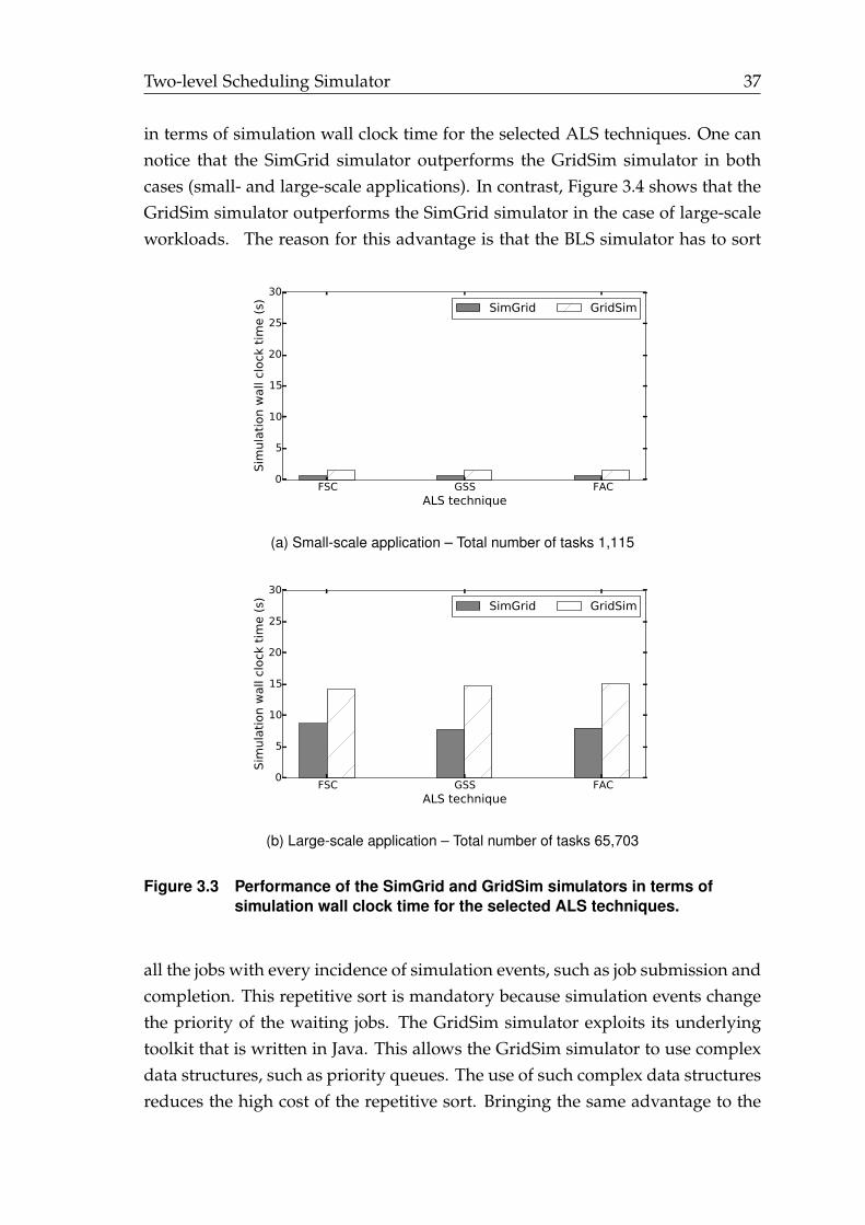
Two-level Scheduling Simulator 37
in terms of simulation wall clock time for the selected ALS techniques. One cannotice that the SimGrid simulator outperforms the GridSim simulator in bothcases (small- and large-scale applications). In contrast, Figure 3.4 shows that theGridSim simulator outperforms the SimGrid simulator in the case of large-scaleworkloads. The reason for this advantage is that the BLS simulator has to sort
FSC GSS FACALS technique
0
5
10
15
20
25
30
Sim
ula
tion w
all
clock
tim
e (
s) SimGrid GridSim
(a) Small-scale application – Total number of tasks 1,115
FSC GSS FACALS technique
0
5
10
15
20
25
30
Sim
ula
tion w
all
clock
tim
e (
s) SimGrid GridSim
(b) Large-scale application – Total number of tasks 65,703
Figure 3.3 Performance of the SimGrid and GridSim simulators in terms ofsimulation wall clock time for the selected ALS techniques.
all the jobs with every incidence of simulation events, such as job submission andcompletion. This repetitive sort is mandatory because simulation events changethe priority of the waiting jobs. The GridSim simulator exploits its underlyingtoolkit that is written in Java. This allows the GridSim simulator to use complexdata structures, such as priority queues. The use of such complex data structuresreduces the high cost of the repetitive sort. Bringing the same advantage to the
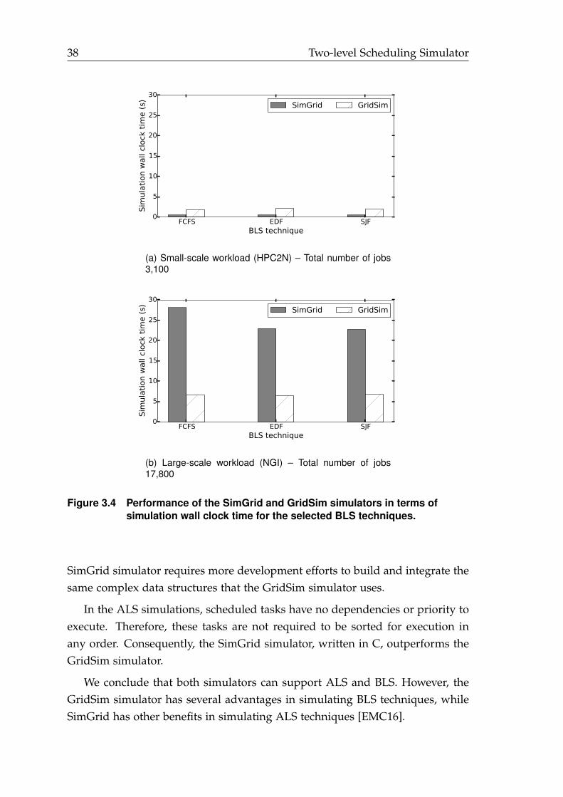
38 Two-level Scheduling Simulator
FCFS EDF SJFBLS technique
0
5
10
15
20
25
30
Sim
ula
tion w
all
clock
tim
e (
s) SimGrid GridSim
(a) Small-scale workload (HPC2N) – Total number of jobs3,100
FCFS EDF SJFBLS technique
0
5
10
15
20
25
30
Sim
ula
tion w
all
clock
tim
e (
s) SimGrid GridSim
(b) Large-scale workload (NGI) – Total number of jobs17,800
Figure 3.4 Performance of the SimGrid and GridSim simulators in terms ofsimulation wall clock time for the selected BLS techniques.
SimGrid simulator requires more development efforts to build and integrate thesame complex data structures that the GridSim simulator uses.
In the ALS simulations, scheduled tasks have no dependencies or priority toexecute. Therefore, these tasks are not required to be sorted for execution inany order. Consequently, the SimGrid simulator, written in C, outperforms theGridSim simulator.
We conclude that both simulators can support ALS and BLS. However, theGridSim simulator has several advantages in simulating BLS techniques, whileSimGrid has other benefits in simulating ALS techniques [EMC16].
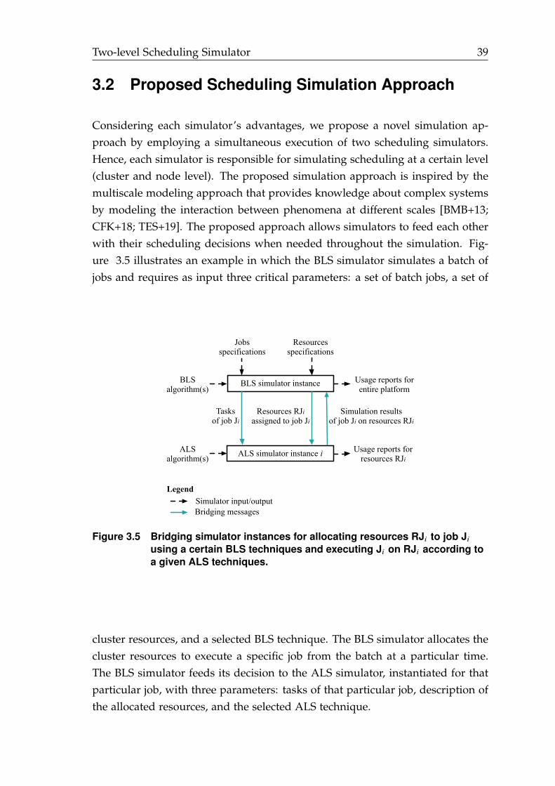
Two-level Scheduling Simulator 39
3.2 Proposed Scheduling Simulation Approach
Considering each simulator’s advantages, we propose a novel simulation ap-proach by employing a simultaneous execution of two scheduling simulators.Hence, each simulator is responsible for simulating scheduling at a certain level(cluster and node level). The proposed simulation approach is inspired by themultiscale modeling approach that provides knowledge about complex systemsby modeling the interaction between phenomena at different scales [BMB+13;CFK+18; TES+19]. The proposed approach allows simulators to feed each otherwith their scheduling decisions when needed throughout the simulation. Fig-ure 3.5 illustrates an example in which the BLS simulator simulates a batch ofjobs and requires as input three critical parameters: a set of batch jobs, a set of
BLS simulator instance
Jobs specifications
Resourcesspecifications
BLSalgorithm(s)
Tasks of job Ji
Resources RJi assigned to job Ji
ALS simulator instance i
Simulation resultsof job Ji on resources RJi
ALSalgorithm(s)
Usage reports forentire platform
Usage reports for resources RJi
LegendSimulator input/outputBridging messages
Figure 3.5 Bridging simulator instances for allocating resources RJi to job Ji
using a certain BLS techniques and executing Ji on RJi according toa given ALS techniques.
cluster resources, and a selected BLS technique. The BLS simulator allocates thecluster resources to execute a specific job from the batch at a particular time.The BLS simulator feeds its decision to the ALS simulator, instantiated for thatparticular job, with three parameters: tasks of that particular job, description ofthe allocated resources, and the selected ALS technique.
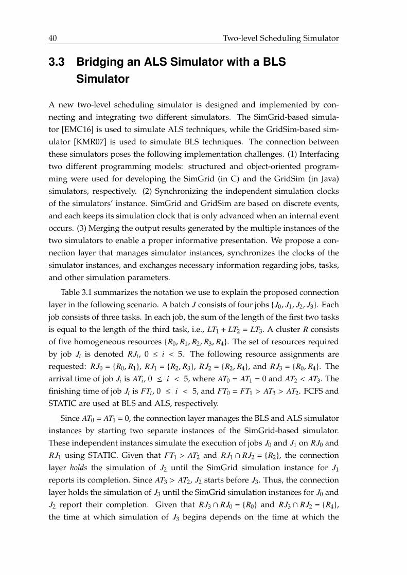
40 Two-level Scheduling Simulator
3.3 Bridging an ALS Simulator with a BLSSimulator
A new two-level scheduling simulator is designed and implemented by con-necting and integrating two different simulators. The SimGrid-based simula-tor [EMC16] is used to simulate ALS techniques, while the GridSim-based sim-ulator [KMR07] is used to simulate BLS techniques. The connection betweenthese simulators poses the following implementation challenges. (1) Interfacingtwo different programming models: structured and object-oriented program-ming were used for developing the SimGrid (in C) and the GridSim (in Java)simulators, respectively. (2) Synchronizing the independent simulation clocksof the simulators’ instance. SimGrid and GridSim are based on discrete events,and each keeps its simulation clock that is only advanced when an internal eventoccurs. (3) Merging the output results generated by the multiple instances of thetwo simulators to enable a proper informative presentation. We propose a con-nection layer that manages simulator instances, synchronizes the clocks of thesimulator instances, and exchanges necessary information regarding jobs, tasks,and other simulation parameters.
Table 3.1 summarizes the notation we use to explain the proposed connectionlayer in the following scenario. A batch J consists of four jobs {J0, J1, J2, J3}. Eachjob consists of three tasks. In each job, the sum of the length of the first two tasksis equal to the length of the third task, i.e., LT1 + LT2 = LT3. A cluster R consistsof five homogeneous resources {R0, R1, R2, R3, R4}. The set of resources requiredby job Ji is denoted RJi, 0 ≤ i < 5. The following resource assignments arerequested: RJ0 = {R0, R1}, RJ1 = {R2, R3}, RJ2 = {R2, R4}, and RJ3 = {R0, R4}. Thearrival time of job Ji is ATi, 0 ≤ i < 5, where AT0 = AT1 = 0 and AT2 < AT3. Thefinishing time of job Ji is FTi, 0 ≤ i < 5, and FT0 = FT1 > AT3 > AT2. FCFS andSTATIC are used at BLS and ALS, respectively.
Since AT0 = AT1 = 0, the connection layer manages the BLS and ALS simulatorinstances by starting two separate instances of the SimGrid-based simulator.These independent instances simulate the execution of jobs J0 and J1 on RJ0 andRJ1 using STATIC. Given that FT1 > AT2 and RJ1 ∩ RJ2 = {R2}, the connectionlayer holds the simulation of J2 until the SimGrid simulation instance for J1
reports its completion. Since AT3 > AT2, J2 starts before J3. Thus, the connectionlayer holds the simulation of J3 until the SimGrid simulation instances for J0 andJ2 report their completion. Given that RJ3 ∩ RJ0 = {R0} and RJ3 ∩ RJ2 = {R4},the time at which simulation of J3 begins depends on the time at which the
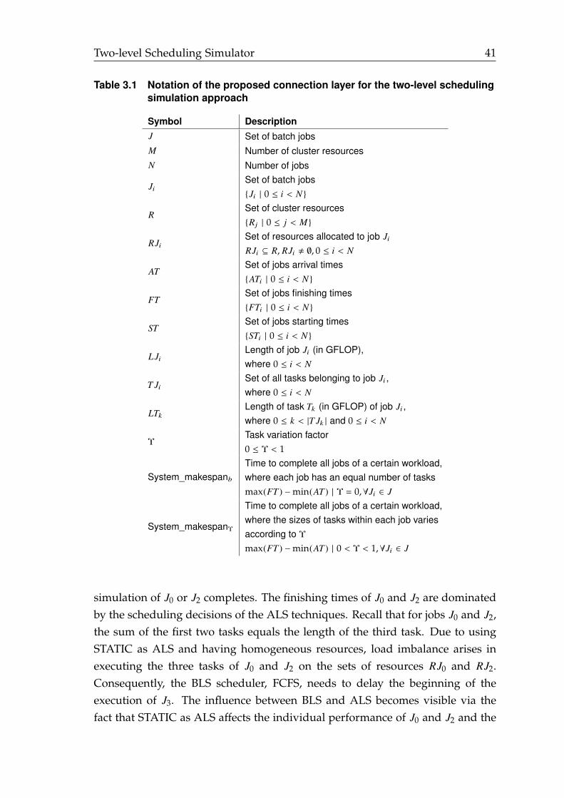
Two-level Scheduling Simulator 41
Table 3.1 Notation of the proposed connection layer for the two-level schedulingsimulation approach
Symbol DescriptionJ Set of batch jobsM Number of cluster resourcesN Number of jobs
JiSet of batch jobs{Ji | 0 ≤ i < N }
RSet of cluster resources{Rj | 0 ≤ j < M }
RJiSet of resources allocated to job JiRJi ⊆ R, RJi , ∅, 0 ≤ i < N
ATSet of jobs arrival times{ATi | 0 ≤ i < N }
FTSet of jobs finishing times{FTi | 0 ≤ i < N }
STSet of jobs starting times{STi | 0 ≤ i < N }
LJiLength of job Ji (in GFLOP),where 0 ≤ i < N
T JiSet of all tasks belonging to job Ji ,where 0 ≤ i < N
LTkLength of task Tk (in GFLOP) of job Ji ,where 0 ≤ k < |T Jk | and 0 ≤ i < N
ΥTask variation factor0 ≤ Υ < 1
System_makespanb
Time to complete all jobs of a certain workload,where each job has an equal number of tasksmax(FT ) −min(AT ) | Υ = 0,∀Ji ∈ J
System_makespanΥ
Time to complete all jobs of a certain workload,where the sizes of tasks within each job variesaccording to Υmax(FT ) −min(AT ) | 0 < Υ < 1,∀Ji ∈ J
simulation of J0 or J2 completes. The finishing times of J0 and J2 are dominatedby the scheduling decisions of the ALS techniques. Recall that for jobs J0 and J2,the sum of the first two tasks equals the length of the third task. Due to usingSTATIC as ALS and having homogeneous resources, load imbalance arises inexecuting the three tasks of J0 and J2 on the sets of resources RJ0 and RJ2.Consequently, the BLS scheduler, FCFS, needs to delay the beginning of theexecution of J3. The influence between BLS and ALS becomes visible via thefact that STATIC as ALS affects the individual performance of J0 and J2 and the

42 Two-level Scheduling Simulator
performance achieved by FCFS, as well. In this scenario, if the FCFS techniquepassed certain information to the STATIC technique to prioritize the release ofresources, the STATIC technique would assign the smallest chunk of tasks to theresources needed to be released for other jobs, such as R0 and R4.
The connection layer synchronizes the running simulators using two strate-gies: simulation suspend/resume and event injection, as illustrated in Figure 3.6.A simulation suspend/resume entity registered in GridSim-based is used to sus-pend and resume the BLS simulation. It performs a busy loop that ends if andonly if all running instances of the SimGrid-based simulator report their com-pletion and results. Because the suspend entity is a registered GridSim entity, itsbusy loop can pause the simulation clock of the GridSim-based simulator untilthe busy loop ends.
SimGrid-SD simulation process SimGrid-SD simulation process
Job completion
GridSim-Alea simulation process
Suspend simulation
Job execution report
Execution report
Starting parameters
Execution report
Job submission
Legend
Job loader entity
GridSim simulation engine
Scheduler entity
Simulation suspend/resume
entity
Job submission
Job submission
BLScommunication
manager
GridSim entityregistration
Job execution update
Job execution report
GridSim entityregistration
GridSim entityregistration
ALS communication
manager
Job simulation using given ALS on allocated resources
Internal GridSim events
Internal synchronization events of the connection layerConnection layer entities
External messages of the connection layer
BLS simulator instance
ALS simulator instance 1 ALS simulator instance N
. . .
Job execution update
Starting parameters
Job simulation using given ALS on allocated resources
ALS communication
manager
Simulation clock within a simulation instance
Figure 3.6 The two-level scheduling simulator. The two-level simulator consists ofa single BLS and several ALS simulation instances. The connection layersynchronizes the independent simulation clocks of the GridSim andSimGrid simulators.
The internal synchronization events in Figure 3.6 are created by the BLS com-munication manager and used to update the simulation suspend/resume entity.
Two-level Scheduling Simulator 43
Thus, the suspend/resume entity can incrementally inject the execution reportsof the running SimGrid simulation instances into the GridSim engine (see Figure3.6). Furthermore, the suspend/resume entity can end the GridSim engine busyloop when there are no more running SimGrid simulation instances. The sim-ulation suspend/resume entity injects the execution reports as GridSim events.Therefore, the GridSim engine can use them to advance its simulation clock.Figure 3.6 depicts the GridSim and SimGrid simulators’ independent simula-tion clocks and their synchronization by connection layer..
The connection layer uses socket-based communication and application ar-guments to exchange the information between the GridSim simulator and theSimGrid simulator instances. The connection layer launches SimGrid simulatorinstances as independent application processes and passes certain parameters asapplication arguments to each established process.
3.4 From High Level to Detailed HPC WorkloadRepresentation
A holistic simulation of ALS and BLS requires information relevant to both lev-els. For the available HPC workloads [FTK14], it is often the case of keepingonly the information relevant to BLS. The workloads in PWA [Fei05] only keepsinformation such as job ID, submission time, wait time, allocated resources anduser ID. Additional details regarding the ALS are essential. For instance, ALSsimulations require details regarding the characteristics of the application andthe number of parallel tasks within the application.
Since this information is not presented in the PWA workloads, we make thefollowing assumptions:
1. All jobs in the workload are computationally-intensive. Consequently, allcommunication or I/O tasks that may exist in the original jobs are notconsidered. This assumption is not a limitation of the proposed approach.It is simply used to convert the existing workloads to one of the possiblecases where jobs are computationally-intensive, as such jobs are among themain incentives for using HPC systems.
2. Although the number of tasks and the length of each task are application-dependent, we consider the case of ideal parallelism. All available hard-ware parallelism is exploited, execution is perfectly load balanced, com-munication is virtually instantaneous, and the resources allocated to tasks
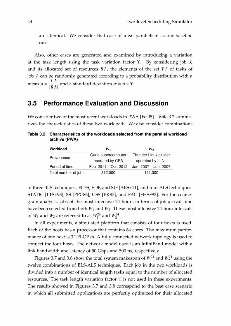
44 Two-level Scheduling Simulator
are identical. We consider that case of ideal parallelism as our baselinecase.
Also, other cases are generated and examined by introducing a variationat the task length using the task variation factor Υ. By considering job Ji
and its allocated set of resources RJi, the elements of the set T Ji of tasks ofjob Ji can be randomly generated according to a probability distribution with a
mean µ =LJi
|RJi |and a standard deviation σ = µ×Υ.
3.5 Performance Evaluation and Discussion
We consider two of the most recent workloads in PWA [Fei05]. Table 3.2 summa-rizes the characteristics of these two workloads. We also consider combinations
Table 3.2 Characteristics of the workloads selected from the parallel workloadarchive (PWA)
Workload W1 W2
ProvenanceCurie supercomputer
operated by CEAThunder Linux cluster
operated by LLNLPeriod of time Feb, 2011 – Oct, 2012 Jan, 2007 – Jun, 2007Total number of jobs 312,000 121,000
of three BLS techniques: FCFS, EDF, and SJF [ABS+11], and four ALS techniques:STATIC [LTS+93], SS [PPC86], GSS [PK87], and FAC [FHSF92]. For the coarse-grain analysis, jobs of the most intensive 24 hours in terms of job arrival timehave been selected from both W1 and W2. These most intensive 24-hour intervalsof W1 and W2 are referred to as W 24
1 and W 242 .
In all experiments, a simulated platform that consists of four hosts is used.Each of the hosts has a processor that contains 64 cores. The maximum perfor-mance of one host is 3 TFLOP/s. A fully connected network topology is used toconnect the four hosts. The network model used is an InfiniBand model with alink bandwidth and latency of 50 Gbps and 500 ns, respectively.
Figures 3.7 and 3.8 show the total system makespan of W 241 and W 24
2 using thetwelve combinations of BLS-ALS techniques. Each job in the two workloads isdivided into a number of identical length tasks equal to the number of allocatedresources. The task length variation factor Υ is not used in these experiments.The results showed in Figures 3.7 and 3.8 correspond to the best case scenarioin which all submitted applications are perfectly optimized for their allocated
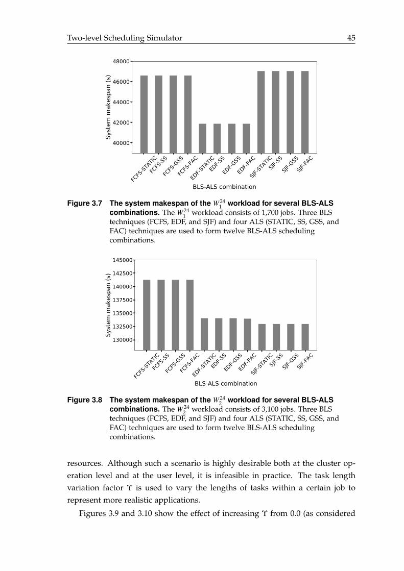
Two-level Scheduling Simulator 45
FCFS
-STATIC
FCFS
-SS
FCFS
-GSS
FCFS
-FAC
EDF-S
TATICED
F-SS
EDF-G
SS
EDF-F
AC
SJF-ST
ATICSJF
-SS
SJF-GSS
SJF-FA
C
BLS-ALS combination
40000
42000
44000
46000
48000
Syst
em m
akes
pan
(s)
Figure 3.7 The system makespan of the W 241 workload for several BLS-ALS
combinations. The W 241 workload consists of 1,700 jobs. Three BLS
techniques (FCFS, EDF, and SJF) and four ALS (STATIC, SS, GSS, andFAC) techniques are used to form twelve BLS-ALS schedulingcombinations.
FCFS
-STATIC
FCFS
-SS
FCFS
-GSS
FCFS
-FAC
EDF-S
TATICED
F-SS
EDF-G
SS
EDF-F
AC
SJF-ST
ATICSJF
-SS
SJF-GSS
SJF-FA
C
BLS-ALS combination
130000
132500
135000
137500
140000
142500
145000
Syst
em m
akes
pan
(s)
Figure 3.8 The system makespan of the W 242 workload for several BLS-ALS
combinations. The W 242 workload consists of 3,100 jobs. Three BLS
techniques (FCFS, EDF, and SJF) and four ALS (STATIC, SS, GSS, andFAC) techniques are used to form twelve BLS-ALS schedulingcombinations.
resources. Although such a scenario is highly desirable both at the cluster op-eration level and at the user level, it is infeasible in practice. The task lengthvariation factor Υ is used to vary the lengths of tasks within a certain job torepresent more realistic applications.
Figures 3.9 and 3.10 show the effect of increasing Υ from 0.0 (as considered
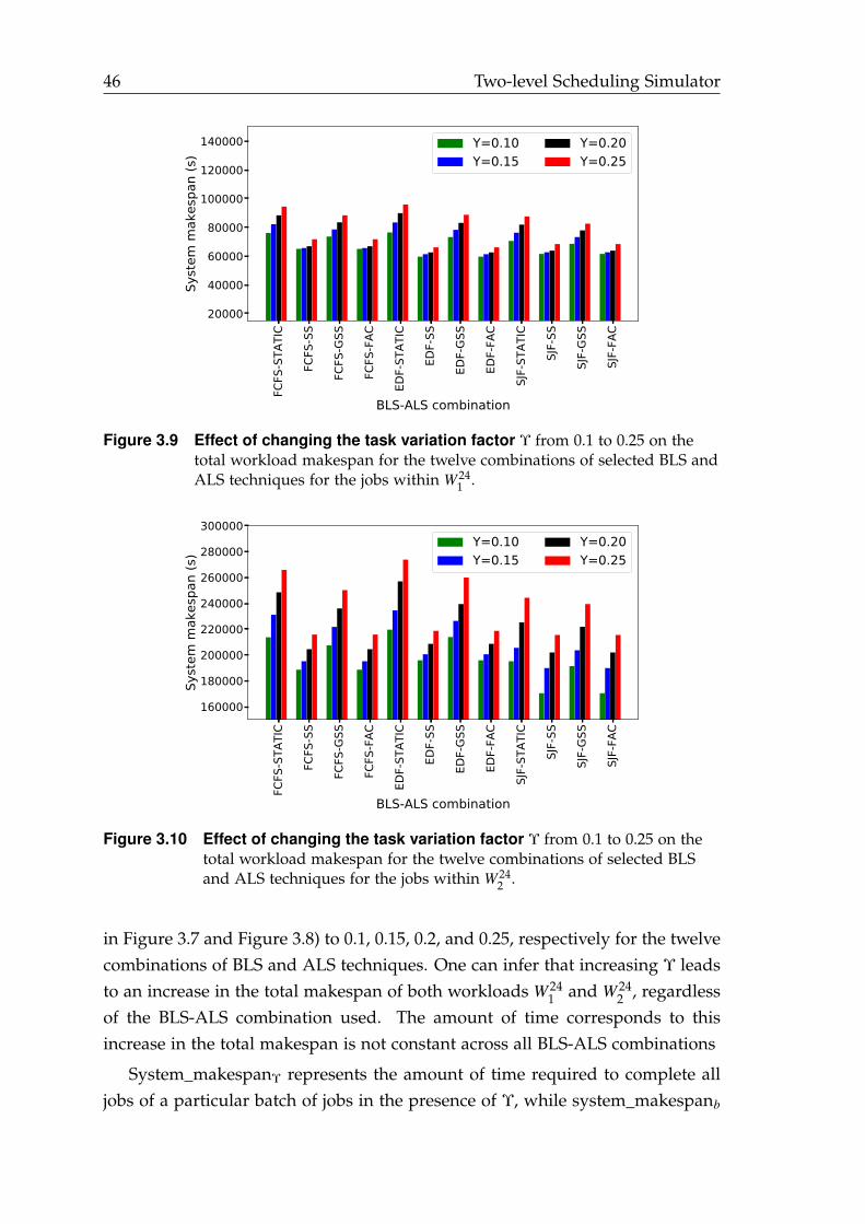
46 Two-level Scheduling Simulator
FCFS
-STA
TIC
FCFS
-SS
FCFS
-GSS
FCFS
-FAC
EDF-
STAT
IC
EDF-
SS
EDF-
GSS
EDF-
FAC
SJF-
STAT
IC
SJF-
SS
SJF-
GSS
SJF-
FAC
BLS-ALS combination
20000
40000
60000
80000
100000
120000
140000
Syst
em m
akes
pan
(s)
=0.10=0.15
=0.20=0.25
Figure 3.9 Effect of changing the task variation factor Υ from 0.1 to 0.25 on thetotal workload makespan for the twelve combinations of selected BLS andALS techniques for the jobs within W 24
1 .
FCFS
-STA
TIC
FCFS
-SS
FCFS
-GSS
FCFS
-FAC
EDF-
STAT
IC
EDF-
SS
EDF-
GSS
EDF-
FAC
SJF-
STAT
IC
SJF-
SS
SJF-
GSS
SJF-
FAC
BLS-ALS combination
160000
180000
200000
220000
240000
260000
280000
300000
Syst
em m
akes
pan
(s)
=0.10=0.15
=0.20=0.25
Figure 3.10 Effect of changing the task variation factor Υ from 0.1 to 0.25 on thetotal workload makespan for the twelve combinations of selected BLSand ALS techniques for the jobs within W 24
2 .
in Figure 3.7 and Figure 3.8) to 0.1, 0.15, 0.2, and 0.25, respectively for the twelvecombinations of BLS and ALS techniques. One can infer that increasing Υ leadsto an increase in the total makespan of both workloads W 24
1 and W 242 , regardless
of the BLS-ALS combination used. The amount of time corresponds to thisincrease in the total makespan is not constant across all BLS-ALS combinations
System_makespanΥ represents the amount of time required to complete alljobs of a particular batch of jobs in the presence of Υ, while system_makespanb
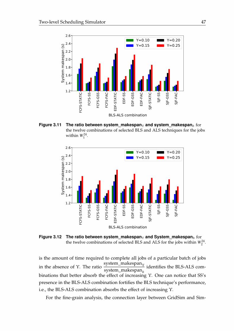
Two-level Scheduling Simulator 47
FCFS
-STA
TIC
FCFS
-SS
FCFS
-GSS
FCFS
-FAC
EDF-
STAT
IC
EDF-
SS
EDF-
GSS
EDF-
FAC
SJF-
STAT
IC
SJF-
SS
SJF-
GSS
SJF-
FAC
BLS-ALS combination
1.2
1.4
1.6
1.8
2.0
2.2
2.4
2.6
Syst
em m
akes
pan
(s)
=0.10=0.15
=0.20=0.25
Figure 3.11 The ratio between system_makespanΥ and system_makespanb forthe twelve combinations of selected BLS and ALS techniques for the jobswithin W 24
1 .
FCFS
-STA
TIC
FCFS
-SS
FCFS
-GSS
FCFS
-FAC
EDF-
STAT
IC
EDF-
SS
EDF-
GSS
EDF-
FAC
SJF-
STAT
IC
SJF-
SS
SJF-
GSS
SJF-
FAC
BLS-ALS combination
1.2
1.4
1.6
1.8
2.0
2.2
2.4
2.6
Syst
em m
akes
pan
(s)
=0.10=0.15
=0.20=0.25
Figure 3.12 The ratio between system_makespanΥ and System_makespanb forthe twelve combinations of selected BLS and ALS for the jobs within W 24
2 .
is the amount of time required to complete all jobs of a particular batch of jobs
in the absence of Υ. The ratiosystem_makespan
Υ
system_makespanbidentifies the BLS-ALS com-
binations that better absorb the effect of increasing Υ. One can notice that SS’spresence in the BLS-ALS combination fortifies the BLS technique’s performance,i.e., the BLS-ALS combination absorbs the effect of increasing Υ.
For the fine-grain analysis, the connection layer between GridSim and Sim-
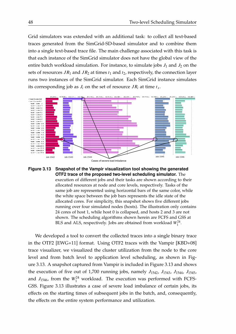
48 Two-level Scheduling Simulator
Grid simulators was extended with an additional task: to collect all text-basedtraces generated from the SimGrid-SD-based simulator and to combine theminto a single text-based trace file. The main challenge associated with this task isthat each instance of the SimGrid simulator does not have the global view of theentire batch workload simulation. For instance, to simulate jobs J1 and J2 on thesets of resources JR1 and JR2 at times t1 and t2, respectively, the connection layerruns two instances of the SimGrid simulator. Each SimGrid instance simulatesits corresponding job as Ji on the set of resource JRi at time tx .
Cases of severe load imbalance Job1542 Job1543 Job1544 Job1545 Job1546
Figure 3.13 Snapshot of the Vampir visualization tool showing the generatedOTF2 trace of the proposed two-level scheduling simulator. Theexecution of different jobs and their tasks are shown according to theirallocated resources at node and core levels, respectively. Tasks of thesame job are represented using horizontal bars of the same color, whilethe white space between the job bars represents the idle state of theallocated cores. For simplicity, this snapshot shows five different jobsrunning over four simulated nodes (hosts). The illustration only contains24 cores of host 1, while host 0 is collapsed, and hosts 2 and 3 are notshown. The scheduling algorithms shown herein are FCFS and GSS atBLS and ALS, respectively. Jobs are obtained from workload W 24
1 .
We developed a tool to convert the collected traces into a single binary tracein the OTF2 [EWG+11] format. Using OTF2 traces with the Vampir [KBD+08]trace visualizer, we visualized the cluster utilization from the node to the corelevel and from batch level to application level scheduling, as shown in Fig-ure 3.13. A snapshot captured from Vampir is included in Figure 3.13 and showsthe execution of five out of 1,700 running jobs, namely J1542, J1543, J1544, J1545,and J1546, from the W 24
1 workload. The execution was performed with FCFS-GSS. Figure 3.13 illustrates a case of severe load imbalance of certain jobs, itseffects on the starting times of subsequent jobs in the batch, and, consequently,the effects on the entire system performance and utilization.
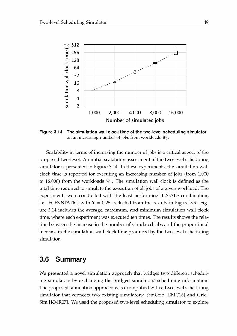
Two-level Scheduling Simulator 49
248163264128256512
1,000 2,000 4,000 8,000 16,000
Simulationwallclocktime(s)
Numberofsimulatedjobs
Figure 3.14 The simulation wall clock time of the two-level scheduling simulatoron an increasing number of jobs from workloads W1.
Scalability in terms of increasing the number of jobs is a critical aspect of theproposed two-level. An initial scalability assessment of the two-level schedulingsimulator is presented in Figure 3.14. In these experiments, the simulation wallclock time is reported for executing an increasing number of jobs (from 1,000to 16,000) from the workloads W1. The simulation wall clock is defined as thetotal time required to simulate the execution of all jobs of a given workload. Theexperiments were conducted with the least performing BLS-ALS combination,i.e., FCFS-STATIC, with Υ = 0.25. selected from the results in Figure 3.9. Fig-ure 3.14 includes the average, maximum, and minimum simulation wall clocktime, where each experiment was executed ten times. The results shows the rela-tion between the increase in the number of simulated jobs and the proportionalincrease in the simulation wall clock time produced by the two-level schedulingsimulator.
3.6 Summary
We presented a novel simulation approach that bridges two different schedul-ing simulators by exchanging the bridged simulators’ scheduling information.The proposed simulation approach was exemplified with a two-level schedulingsimulator that connects two existing simulators: SimGrid [EMC16] and Grid-Sim [KMR07]. We used the proposed two-level scheduling simulator to explore

50 Two-level Scheduling Simulator
twelve combinations of 4 ALS techniques and 3 BLS techniques. We concludethat ALS techniques affect the performance of their applications and the perfor-mance of the entire batch system. Hence, the overall performance of any givenBLS technique is affected by the load imbalance at every individual job.
This conclusion guides our work into the following directions: (1) avoidingor minimizing load imbalance, and if it is not avoidable, (2) exploiting loadimbalance. The first direction is covered by the work presented in Chapters 4and 5, and the second direction is covered by the work presented in Chapter 6.
4Distributed Chunk CalculationApproach (DCA)
The advancements in modern HPC systems at both hardware and software lev-els raise questions regarding the benefits of these advancements for successfultechniques proposed in the past. We need to revisit and re-evaluate these tech-niques to fully leverage modern HPC systems’ capabilities at both hardwareand software levels. As discussed in Chapter 1, we focus on DLS techniquesat the application level. We showed in Chapter 3 that DLS techniques have asubstantial impact on application performance and batch system performance.
This chapter examines the typical execution approaches for DLS techniques,specifically the master-worker execution model. We discuss the influence ofcentralizing the chunk calculation at the master on the DLS techniques’ perfor-mance. Motivated by the advancements in the MPI [For20] standard, we proposea distributed chunk calculation approach (DCA) [EC19a] to eliminate the use ofthe master-worker model. The DCA contributes to our envisioned MLS solutionby minimizing the idle time of computing resources.
4.1 Execution Models of DLS Techniques
The self-scheduling aspect is the distinguishing aspect of all DLS techniques.Self-scheduling means that once a PE becomes free, it calculates a new chunkof loop iterations to be executed. The calculated chunk size is not associatedwith a specific set of loop iterations. The PE must synchronize with all otherPEs to map the calculated chunk size to a specific set of unscheduled loop it-erations. There are two operations at every scheduling step: chunk calculation
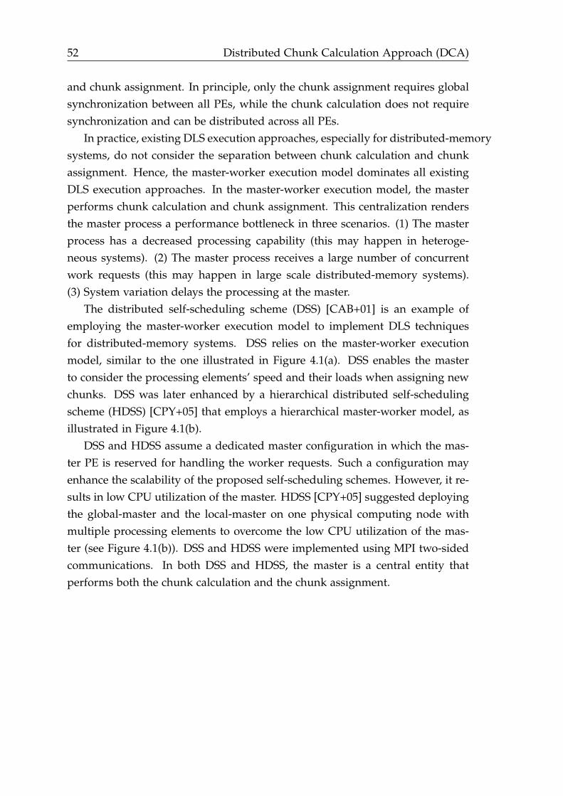
52 Distributed Chunk Calculation Approach (DCA)
and chunk assignment. In principle, only the chunk assignment requires globalsynchronization between all PEs, while the chunk calculation does not requiresynchronization and can be distributed across all PEs.
In practice, existing DLS execution approaches, especially for distributed-memorysystems, do not consider the separation between chunk calculation and chunkassignment. Hence, the master-worker execution model dominates all existingDLS execution approaches. In the master-worker execution model, the masterperforms chunk calculation and chunk assignment. This centralization rendersthe master process a performance bottleneck in three scenarios. (1) The masterprocess has a decreased processing capability (this may happen in heteroge-neous systems). (2) The master process receives a large number of concurrentwork requests (this may happen in large scale distributed-memory systems).(3) System variation delays the processing at the master.
The distributed self-scheduling scheme (DSS) [CAB+01] is an example ofemploying the master-worker execution model to implement DLS techniquesfor distributed-memory systems. DSS relies on the master-worker executionmodel, similar to the one illustrated in Figure 4.1(a). DSS enables the masterto consider the processing elements’ speed and their loads when assigning newchunks. DSS was later enhanced by a hierarchical distributed self-schedulingscheme (HDSS) [CPY+05] that employs a hierarchical master-worker model, asillustrated in Figure 4.1(b).
DSS and HDSS assume a dedicated master configuration in which the mas-ter PE is reserved for handling the worker requests. Such a configuration mayenhance the scalability of the proposed self-scheduling schemes. However, it re-sults in low CPU utilization of the master. HDSS [CPY+05] suggested deployingthe global-master and the local-master on one physical computing node withmultiple processing elements to overcome the low CPU utilization of the mas-ter (see Figure 4.1(b)). DSS and HDSS were implemented using MPI two-sidedcommunications. In both DSS and HDSS, the master is a central entity thatperforms both the chunk calculation and the chunk assignment.

Distributed Chunk Calculation Approach (DCA) 53
p 0
p 0p 1
p P-1
...
Req
uest
w
ork
Assi
gnw
ork
Assi
gnw
ork
Req
uest
w
ork
(a)
Con
vent
iona
lm
as-
ter
wor
ker
exec
utio
nm
odel
p 0
p 0p k
p P-1
Req
uest
w
ork
Assi
gnw
ork
p 0 p j
p kR
eque
st
wor
k
Assi
gnw
ork
Req
uest
w
ork
Assi
gnw
ork Req
uest
w
ork
Assi
gnw
ork
...
...
(b)
Glo
bala
ndlo
calm
aste
rsar
elo
cate
don
asi
ngle
phys
ical
com
pute
node
p 0p k
p P-1
Req
uest
w
ork
Assi
gnw
ork
p 0 p j
p kR
eque
st
wor
kAs
sign
wor
k
Req
uest
w
ork
Assi
gnw
ork R
eque
st
wor
kAs
sign
wor
k
p 0
...
...
(c)
Loca
lm
aste
rsar
edi
strib
uted
acro
ssm
ultip
leph
ysic
alco
mpu
teno
des
LEG
EN
D Glo
bal m
aste
rLo
cal m
aste
rB
usy
wor
ker
Ava
ilabl
e an
d re
ques
ting
wor
ker
Two-
side
d m
essa
ges
Phy
sica
l com
pute
nod
e
Figu
re4.
1Va
rian
tsof
the
mas
ter-
wor
ker
exec
utio
nm
odel
,as
repo
rted
inth
elit
erat
ure.
Rep
licat
ion
ofce
rtai
npr
oces
sing
elem
ents
isju
stto
indi
cate
thei
rdo
uble
role
whe
reth
em
aste
rpa
rtic
ipat
esin
the
com
puta
tion
asa
wor
ker.
54 Distributed Chunk Calculation Approach (DCA)
Another MPI-based library that implements several DLS techniques is calledthe load balancing tool (LB tool) [CB05]. At the conceptual level, the LB toolis based on a single-level master-worker execution model (see Figure 4.1(a)).However, it does not assume a dedicated master. It introduces the breakAfter(user-defined) parameter and indicates how many iterations the master shouldexecute before serving pending worker requests. This parameter is required fordividing the time of the master between computation and servicing of worker re-quests. The optimal value of this parameter is application- and system-dependent.The LB tool also employs two-sided MPI communications.
LB4MPI [MEC+20; MC20] is an extension of the LB tool [CB05] that includescertain bug fixes and additional DLS techniques. Both LB and LB4MPI employa master-worker execution in which the master is a central entity that performsboth the chunk calculation and the chunk assignment operations.
The dynamic load balancing library (DLBL) [BCP+05] is another MPI-basedlibrary used for cluster computing. It is based on a parallel runtime environ-ment for multicomputer applications (PREMA) [BCC+04]. DLBL is the first toolthat employed MPI one-sided communication for implementing DLS techniques.Similar to the LB tool, the DLBL employs a master-worker execution model. Themaster expects work requests. It then calculates the chunk’s size to be assignedand, subsequently, calls a handler function on the worker side. The worker isresponsible for obtaining the new chunk data without any further involvementfrom the master. This means that the master is still a central entity that performsboth chunk calculation and chunk assignment.
4.2 From Centralized to Decentralized DLSTechniques
The idea of DCA is to ensure that the calculated chunk size at a specific PE doesnot rely on any information about the chunk size calculated at any other PE.The chunk calculation formulas (Eq. 2.1 to 2.13) can be classified into straight-forward and recursive formulas. A straightforward chunk calculation formulaonly requires some constants and input parameters. A recursive chunk calcula-tion formula requires information about previously calculated chunk sizes. Forinstance, STATIC, SS, FSC, and RND have straightforward chunk calculation for-mulas that do not require any information about previously calculated chunks,while GSS [PK87], TAP [Luc92], TSS [TN93], FAC [FHSF92], TFSS [CAB+01],FISS [PD97], VISS [PD97], AF [Ban00], and PLS [SYT07] employ recursive chunk

Distributed Chunk Calculation Approach (DCA) 55
calculation formulas. Certain transformations are required to convert these re-cursive formulas into straightforward formulas to enable DCA. For GSS andFAC, the transformations were already introduced in the literature [FHSF92](Eq. 4.1 and 4.2).
K′GSS
i =
⎡⎢⎢⎢⎢⎢
(P − 1
P
) i
·NP
⎤⎥⎥⎥⎥⎥(4.1)
K′FAC2
i =
⎡⎢⎢⎢⎢⎢
(12
) inew
·NP
⎤⎥⎥⎥⎥⎥, inew =
⌊iP
⌋+ 1 (4.2)
As shown in Eq. 2.5, TAP calculates KGSSi and tunes that value based on µ, σ,
and α. Based on Eq. 4.1, the chunk calculation formula of TSS can be expressedas a straightforward formula as follows.
K′T AP
i = K′GSS
i +v2α
2− vα ·
√2 · K′GSS
i +v2α
4, where
vα =α · σ
µ
(4.3)
For TSS, a straightforward formula for the chunk calculation is shown inEq. 4.4.
K′TSS
i = KT SS0 − i · ⌊
KT SS0 − KT SS
S−1
S − 1⌋ (4.4)
The mathematical derivation that converts Eq. 2.6 into Eq. 4.4 is as follows. TheTSS chunk calculation formula can be represented as follows, where C is a con-stant.
KT SSi = KT SS
i−1 −C
C =⎢⎢⎢⎢⎢⎣
KT SS0 − KT SS
S−1
S − 1
⎥⎥⎥⎥⎥⎦KT SS
1 = KT SS0 −C
KT SS2 = KT SS
1 −C = (KT SS0 −C) −C = KT SS
0 − 2 ·C
KT SSi = KT SS
0 − i ·C
KT SSi = KT SS
0 − i · ⌊KT SS
0 − KT SSS−1
S − 1⌋ = K′
TSS
i
TFSS [CAB+01] is devised based on TSS [TN93] and FAC [FHSF92]. There-fore, the straightforward formula of TSS (see Eq. 2.6) can be used to derive thestraightforward formula of TFSS, as shown in Eq. 4.5.
K′TFSS
i =
∑i+P−1j=i K′
TSS
j
P(4.5)
56 Distributed Chunk Calculation Approach (DCA)
For FISS [PD97], a straightforward formula for the chunk calculation is shownin Eq. 4.6.
K′FISS
i = KFISS0 + i · ⌈
2 · N · (1 − B2+B )
P · B · (B − 1)⌉ (4.6)
The mathematical derivation that converts Eq. 2.10 into Eq. 4.6 is as follows.Given that A is a constant, the FISS chunk calculation formula can be representedas follows, where C is a constant.
KFISSi = KFISS
i−1 +C
C = ⌈2 · N · (1 − B
2+B )P · B · (B − 1)
⌉
KFISS1 = KFISS
0 +C
KFISS2 = KFISS
1 +C = (KFISS0 +C) +C = KFISS
0 + 2 ·C
KFISSi = KFISS
0 + i ·C
KFISSi = KFISS
0 + i · ⌈2 · N · (1 − B
2+B )P · B · (B − 1)
⌉ = K′FISS
i
For VISS [PD97], a straightforward formula for the chunk calculation isshown in Eq. 4.7.
K′V ISS
i = KFISS0 ·
1 − (0.5)inew
0.5, where i > 0
inew = i mod P
K′V ISS
0 = KFISS0
(4.7)
To derive Eq. 4.7, we calculate KV ISS1 , KV ISS
2 , and KV ISS3 , according to Eq. 2.11.
KV ISS1 = KFISS
0 +KFISS
0
2, assume KFISS
0 = a
KV ISS1 = a +
a2
KV ISS2 = KV ISS
1 +KV ISS
1
2= (a +
a2
) + (a + a
2
2)
KV ISS3 = KV ISS
2 +KV ISS
2
2= ((a +
a2
) + (a + a
2
2)) +
((a + a2 ) + ( a+ a
22 ))
2According to the geomertic summation theorem
KV ISSi = KFISS
0 ·1 − (0.5)i
0.5since VISS assigns chunks in batches
KV ISSi = KFISS
0 ·1 − (0.5)inew
0.5= K′
V ISS
i , where i > 0,
and inew = i mod P.
Distributed Chunk Calculation Approach (DCA) 57
For PLS, the loop iteration space is divided into two parts. In the first part,the PLS chunk calculation formula is equivalent to STATIC, i.e., the chunk calcu-lation formula is a straightforward formula that is ready to support DCA. In thesecond part, PLS uses the GSS chunk calculation formula. Therefore, we replaceKGSS
i in Eq. 2.13 with K′GSS
i from Eq. 4.1 to derive the PLS chunk calculation(Eq. 4.8).
K′PLS
i =⎧⎪⎨⎪⎩
N ·SW RP , if Ri > N − (N · SW R)
K′GSS
i , otherwise.(4.8)
AF adapts the calculated chunk size according to µpi and σpi , which can bedetermined only during loop execution. Moreover, at every scheduling step,AF uses Ri with µpi and σpi to calculate the chunk size. This leads to an unpre-dictable pattern of chunk sizes and makes it impossible to find a straightforwardformula for AF. Accordingly, we could not determine a way to implement AFwith a fully distributed chunk calculation. In our implementation, AF with DCArequires additional synchronization of Ri across all PEs. All PEs can simultane-ously calculate D and E from Eq. 2.14. However, each PE needs to synchronizewith all other PEs to calculate each K AF
i .
4.3 Distribution of the Chunk Calculation
In the proposed DCA, we replace the master role with a coordinator role. Thecoordinator holds a central work queue that contains the global scheduling in-formation, such as the last scheduling step i and the last loop index start lpstart.One can consider the value of the last scheduling step i as the only requiredinput parameter for the newly derived chunk calculation formulas (see Sec-tion 4.2). DCA has three major steps:Step 1. Workers synchronize through the coordinator to exclusively get a localcopy of i and increment the global i by one.Step 2. Workers use their local copies of i to calculate their chunk sizes.Step 3. Workers synchronize once again to exclusively get a local copy of the lastloop index start lpstart and increment the global lpstart by the calculated chunksize.At that point, every worker can execute loop iterations from lpstart to lpstart +
the calculated chunk size. In the proposed DCA, the coordinator acts like aworker with one exception that is holding the central work queue.
Figure 4.2 illustrates the DLS execution using the proposed DCA. Processorsp0 and p1 calculate K0 and K1 simultaneously. The time required to calculate K0
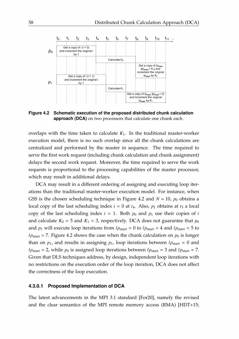
58 Distributed Chunk Calculation Approach (DCA)
t2t1 t3 t4 t5 t6t0
p0
p1
Get a copy of i (i = 0)and increment the original i
by 1
Get a copy of i (i = 1)and increment the original i
by 1
Calculate K0
Calculate K1
Get a copy of lpstart (lpstart= 0)and increment the original
lpstart by K1
Get a copy of lpstart(lpstart= K1) and
increment the original lpstart by K0
t7 t8 t9 t10 t11 …
Figure 4.2 Schematic execution of the proposed distributed chunk calculationapproach (DCA) on two processors that calculate one chunk each.
overlaps with the time taken to calculate K1. In the traditional master-workerexecution model, there is no such overlap since all the chunk calculations arecentralized and performed by the master in sequence. The time required toserve the first work request (including chunk calculation and chunk assignment)delays the second work request. Moreover, the time required to serve the workrequests is proportional to the processing capabilities of the master processor,which may result in additional delays.
DCA may result in a different ordering of assigning and executing loop iter-ations than the traditional master-worker execution model. For instance, whenGSS is the chosen scheduling technique in Figure 4.2 and N = 10, p0 obtains alocal copy of the last scheduling index i = 0 at t4. Also, p1 obtains at t5 a localcopy of the last scheduling index i = 1. Both p0 and p1 use their copies of i
and calculate K0 = 5 and K1 = 3, respectively. DCA does not guarantee that p0
and p1 will execute loop iterations from lpstart = 0 to lpstart = 4 and lpstart = 5 tolpstart = 7. Figure 4.2 shows the case when the chunk calculation on p0 is longerthan on p1, and results in assigning p1, loop iterations between lpstart = 0 andlpstart = 2, while p0 is assigned loop iterations between lpstart = 3 and lpstart = 7.Given that DLS techniques address, by design, independent loop iterations withno restrictions on the execution order of the loop iteration, DCA does not affectthe correctness of the loop execution.
4.3.0.1 Proposed Implementation of DCA
The latest advancements in the MPI 3.1 standard [For20], namely the revisedand the clear semantics of the MPI remote memory access (RMA) [HDT+15;

Distributed Chunk Calculation Approach (DCA) 59
ZBG16], enabled its usage in different scientific applications [HGC14; SWZ+16;ZG16]. The MPI RMA model, also known as one-sided communication, pro-vides the necessary function calls to implement the proposed DCA. In the MPIRMA model, each process’s memory is by default private, and other processescannot directly access it. The MPI RMA model allows MPI processes to exposedifferent regions of their memory, called windows. One MPI process (origin) candirectly access a memory window without any involvement of the other (target)process that owns the window.
The MPI RMA has two synchronization modes: passive- and active-target. Inthe active-target synchronization, the target process determines the time bound-aries, called epochs, when its window can be accessed. In the passive-targetsynchronization, the target process has no time limits when its window canbe accessed. The DCA can benefit from the passive-target synchronization be-cause it requires a minimal amount of synchronization, and it efficiently allowsthe most significant overlap of computation and communication. Moreover, ityields the development of DLS techniques for distributed-memory systems tobe very similar to their original implementations for shared-memory systems.
Figure 4.3 illustrates the main steps of the proposed DCA as follows. (1) theprocessing element p j obtains a copy of the last scheduling step index, i, andatomically increments the global i by one. (2) p j only uses its local copy of i
(before the increment) to calculate Ki with the new derived straightforwardformulas for the selected DLS technique. (3) p j obtains a copy of the lastloop index start, lpstart, and atomically accumulates the size of the calculated
p0 p1p0 pp-1...
Last scheduling step i
(1)Get a copy of iand increment the original i by 1
(3) Get a copy of lpstartand increment the original lpstart
by Ki
(3) Get a copy of lpstartand increment the original lpstart
by Ki
Last start loop index lpstart
(1)Get a copy of iand increment the original i by 1
(2) CalculateKi
(2) Calculate Ki
LEGENDCoordinator
Busy worker Atomic operationsPhysical compute node
Chunk-calculationAvailable and requesting worker Memory region
Memory ownership relation
Figure 4.3 The proposed DCA using MPI RMA and passive-target synchronization.
60 Distributed Chunk Calculation Approach (DCA)
chunk, Ki, into it. Finally, p j executes loop iterations between lpstart (before ac-cumulation) and min(lpstart + Ki, N). The atomic operations in Steps 1 and 3guarantee the exclusive access to i and lpstart. The coordinator MPI processcan use MPI_Win_create to expose the shared variables, such as i and lpstart, toall other MPI processes. The passive-target synchronization mode (MPI_Win_-lock(MPI_LOCK_SHARED)) can be used with certain MPI atomic operations, suchas MPI_Get_accumulate, to grant the exclusive access to i and lpstart by all MPIprocesses.
4.4 Performance Evaluation and Discussion
We evaluated two implementations. The first implementation, denoted One_-
Sided_DLS, employs the proposed DCA, and uses one-sided MPI communicationin the passive-target synchronization mode. The second implementation, de-noted Two_Sided_DLS, employs a master-worker model and uses the two-sidedMPI communication. Both implementations assume a non-dedicated coordina-tor (or a non-dedicated master) processing element.
We considered two computationally-intensive parallel applications in theevaluation. The first application, called PSIA [EFM+16; EMC17a], uses a parallelversion of the well-known spin-image algorithm (SIA) [Joh97]. SIA converts a3D object into a set of 2D images. The generated 2D images can be used asdescriptive features of the 3D object. The second application calculates the Man-delbrot set [Man80]. The Mandelbrot set is used to represent geometric shapesthat have the self-similarity property at various scales. Studying such shapesis essential and of interest in different domains, such as biology, medicine, andchemistry [JTS09].
Both applications contain a single large parallel loop that dominates theirexecution times. Algorithm 4.1 and 4.2 show the pseudocodes of both applica-tions.
Table 4.1 summarizes the execution parameters used for both selected appli-cations. These parameters were selected empirically to guarantee a reasonableaverage iteration execution time that is larger than 0.2 for PISA and 0.02 secondsfor Mandelbrot.
Two types of computing resources are used in our evaluation. The first type,denoted KNL, refers to a standalone Intel Xeon Phi 7210 manycore processorswith 64 cores, 96 GB RAM (flat mode configuration), and 1.3 GHz CPU fre-quency. The second type, denoted Xeon, refers to two-socket Intel Xeon E5-2640
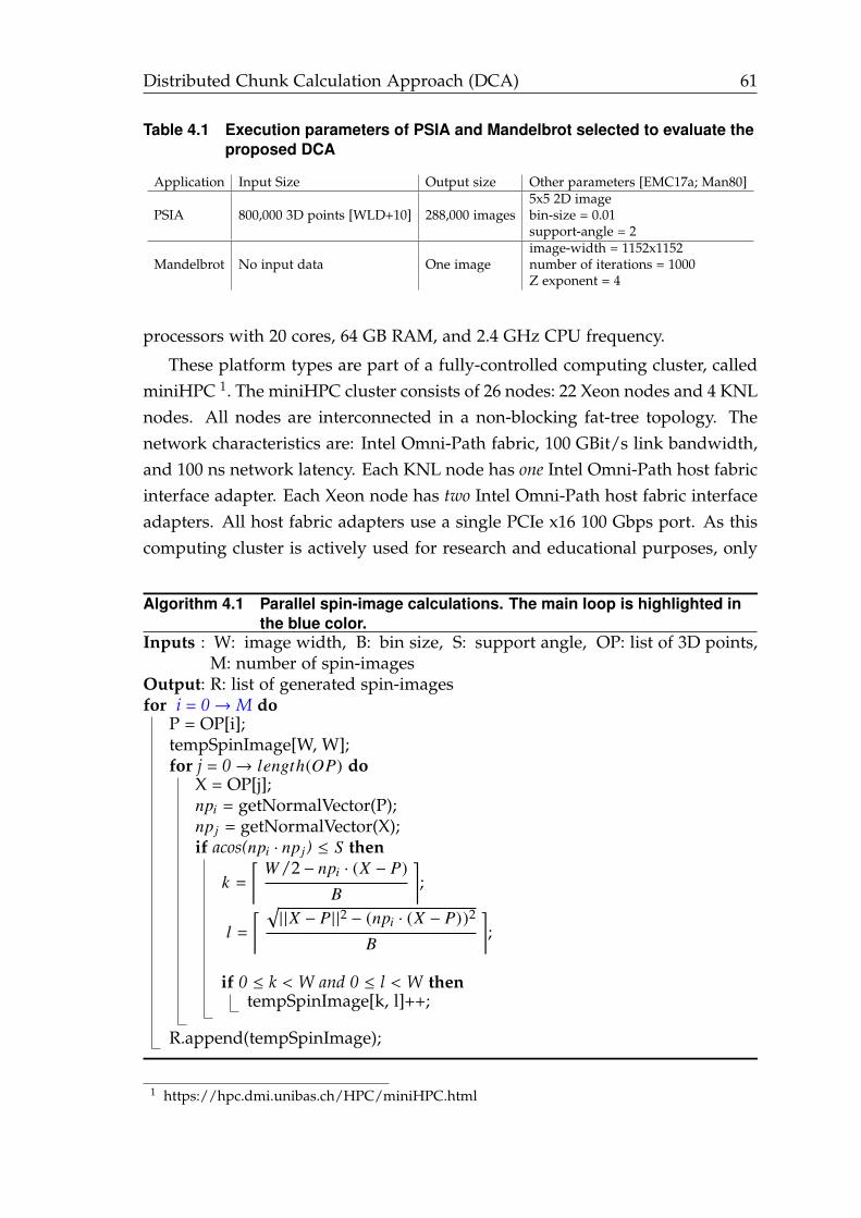
Distributed Chunk Calculation Approach (DCA) 61
Table 4.1 Execution parameters of PSIA and Mandelbrot selected to evaluate theproposed DCA
Application Input Size Output size Other parameters [EMC17a; Man80]
PSIA 800,000 3D points [WLD+10] 288,000 images5x5 2D imagebin-size = 0.01support-angle = 2
Mandelbrot No input data One imageimage-width = 1152x1152number of iterations = 1000Z exponent = 4
processors with 20 cores, 64 GB RAM, and 2.4 GHz CPU frequency.
These platform types are part of a fully-controlled computing cluster, calledminiHPC 1. The miniHPC cluster consists of 26 nodes: 22 Xeon nodes and 4 KNLnodes. All nodes are interconnected in a non-blocking fat-tree topology. Thenetwork characteristics are: Intel Omni-Path fabric, 100 GBit/s link bandwidth,and 100 ns network latency. Each KNL node has one Intel Omni-Path host fabricinterface adapter. Each Xeon node has two Intel Omni-Path host fabric interfaceadapters. All host fabric adapters use a single PCIe x16 100 Gbps port. As thiscomputing cluster is actively used for research and educational purposes, only
Algorithm 4.1 Parallel spin-image calculations. The main loop is highlighted inthe blue color.
Inputs : W: image width, B: bin size, S: support angle, OP: list of 3D points,M: number of spin-images
Output: R: list of generated spin-imagesfor i = 0→M do
P = OP[i];tempSpinImage[W, W];for j = 0→ length(OP) do
X = OP[j];npi = getNormalVector(P);np j = getNormalVector(X);if acos(npi · np j) ≤ S then
k =⌈ W/2 − npi · (X − P)
B
⌉;
l =⌈ √| |X − P | |2 − (npi · (X − P))2
B
⌉;
if 0 ≤ k < W and 0 ≤ l < W thentempSpinImage[k, l]++;
R.append(tempSpinImage);
1 https://hpc.dmi.unibas.ch/HPC/miniHPC.html
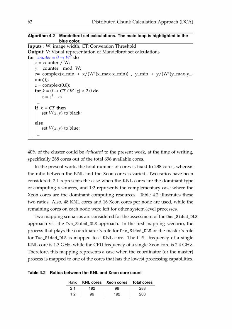
62 Distributed Chunk Calculation Approach (DCA)
Algorithm 4.2 Mandelbrot set calculations. The main loop is highlighted in theblue color.
Inputs : W: image width, CT: Conversion ThresholdOutput: V: Visual representation of Mandelbrot set calculationsfor counter = 0→ W 2 do
x = counter / W;y = counter mod W;c= complex(x_min + x/(W*(x_max-x_min)) , y_min + y/(W*(y_max-y_-min)));z = complex(0,0);for k = 0→ CT OR |z | < 2.0 do
z = z4 + c;
if k = CT thenset V (x, y) to black;
elseset V (x, y) to blue;
40% of the cluster could be dedicated to the present work, at the time of writing,specifically 288 cores out of the total 696 available cores.
In the present work, the total number of cores is fixed to 288 cores, whereasthe ratio between the KNL and the Xeon cores is varied. Two ratios have beenconsidered: 2:1 represents the case when the KNL cores are the dominant typeof computing resources, and 1:2 represents the complementary case where theXeon cores are the dominant computing resources. Table 4.2 illustrates thesetwo ratios. Also, 48 KNL cores and 16 Xeon cores per node are used, while theremaining cores on each node were left for other system-level processes.
Two mapping scenarios are considered for the assessment of the One_Sided_DLSapproach vs. the Two_Sided_DLS approach. In the first mapping scenario, theprocess that plays the coordinator’s role for One_Sided_DLS or the master’s rolefor Two_Sided_DLS is mapped to a KNL core. The CPU frequency of a singleKNL core is 1.3 GHz, while the CPU frequency of a single Xeon core is 2.4 GHz.Therefore, this mapping represents a case when the coordinator (or the master)process is mapped to one of the cores that has the lowest processing capabilities.
Table 4.2 Ratios between the KNL and Xeon core count
Ratio KNL cores Xeon cores Total cores2:1 192 96 2881:2 96 192 288
Distributed Chunk Calculation Approach (DCA) 63
In the second mapping scenario, the process that plays the coordinator’s role (orthe master) is mapped to a Xeon core, which is the most powerful processingelement in the considered system.
Comparing the results of both scenarios shows the adverse impact of re-duced processing capabilities of the master on the performance of the DLStechniques using Two_Sided_DLS. On the contrary, the same mapping for thecoordinator process did not affect the performance of the DLS techniques usingOne_Sided_DLS.
The straightforward parallelization (STATIC) is used as a baseline to assessthe performance of the selected DLS techniques on the target heterogeneouscomputing platform. STATIC assigns ⌈N/P⌉ loop iterations to each processingelement. The considered implementation of STATIC follows the self-schedulingexecution model where every worker obtains a single chunk of size ⌈N/P⌉ loopiterations at the beginning of the application execution. By employing STATIC,the percentage of the parallel execution time of the selected applications’ mainloops T loop
p are 98% and 99.4% of the parallel execution times for PSIA andMandelbrot, respectively. Such high percentages show that the performance ofboth applications is dominated by the execution time of the main loop. Hence,for the remaining results in this section, the analysis concentrates on the parallelloop execution time, T loop
p . All experiments were repeated 20 times, and themedian results are reported in all figures.
For the PSIA application, Figure 4.4(a) shows that SS, GSS, and TSS im-plemented with One_Sided_DLS outperformed their respective versions usingTwo_Sided_DLS. For instance, when the ratio of the KNL cores to the Xeon coreswas 2:1, the parallel loop execution time, T loop
p , of SS required 109 and 233 sec-onds with One_Sided_DLS and Two_Sided_DLS, respectively. Similarly, when theratio was 2:1, the parallel loop execution time, T loop
p , of GSS and TSS increasedfrom 185 and 125 seconds to 236 and 136 seconds, respectively.
When the ratio was 1:2, the total processing capabilities of the system in-creased because the number of Xeon cores increased. However, the parallel loopexecution time, T loop
p , of SS, GSS, and TSS implemented using Two_Sided_DLS
did not take the advantage of increasing the total number of Xeon cores. For in-stance, using One_Sided_DLS, changing the ratio from 2:1 to 1:2 reduced the T loop
p
of SS from 109 to 68.5 seconds. FAC2 and WF behaved similarly using both,One_Sided_DLS and Two_Sided_DLS.
The performance degradation of the DLS techniques with Two_Sided_DLS isdue to mapping the master to a KNL core, which has the lowest processing ca-
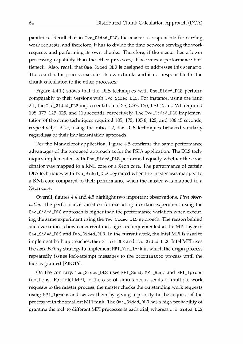
64 Distributed Chunk Calculation Approach (DCA)
pabilities. Recall that in Two_Sided_DLS, the master is responsible for servingwork requests, and therefore, it has to divide the time between serving the workrequests and performing its own chunks. Therefore, if the master has a lowerprocessing capability than the other processes, it becomes a performance bot-tleneck. Also, recall that One_Sided_DLS is designed to addresses this scenario.The coordinator process executes its own chunks and is not responsible for thechunk calculation to the other processes.
Figure 4.4(b) shows that the DLS techniques with One_Sided_DLS performcomparably to their versions with Two_Sided_DLS. For instance, using the ratio2:1, the One_Sided_DLS implementation of SS, GSS, TSS, FAC2, and WF required108, 177, 125, 125, and 110 seconds, respectively. The Two_Sided_DLS implemen-tation of the same techniques required 105, 175, 135.6, 125, and 106.45 seconds,respectively. Also, using the ratio 1:2, the DLS techniques behaved similarlyregardless of their implementation approach.
For the Mandelbrot application, Figure 4.5 confirms the same performanceadvantages of the proposed approach as for the PSIA application. The DLS tech-niques implemented with One_Sided_DLS performed equally whether the coor-dinator was mapped to a KNL core or a Xeon core. The performance of certainDLS techniques with Two_Sided_DLS degraded when the master was mapped toa KNL core compared to their performance when the master was mapped to aXeon core.
Overall, figures 4.4 and 4.5 highlight two important observations. First obser-vation: the performance variation for executing a certain experiment using theOne_Sided_DLS approach is higher than the performance variation when execut-ing the same experiment using the Two_Sided_DLS approach. The reason behindsuch variation is how concurrent messages are implemented at the MPI layer inOne_Sided_DLS and Two_Sided_DLS. In the current work, the Intel MPI is used toimplement both approaches, One_Sided_DLS and Two_Sided_DLS. Intel MPI usesthe Lock Polling strategy to implement MPI_Win_lock in which the origin processrepeatedly issues lock-attempt messages to the coordinator process until thelock is granted [ZBG16].
On the contrary, Two_Sided_DLS uses MPI_Send, MPI_Recv and MPI_Iprobe
functions. For Intel MPI, in the case of simultaneous sends of multiple workrequests to the master process, the master checks the outstanding work requestsusing MPI_Iprobe and serves them by giving a priority to the request of theprocess with the smallest MPI rank. The One_Sided_DLS has a high probability ofgranting the lock to different MPI processes at each trial, whereas Two_Sided_DLS
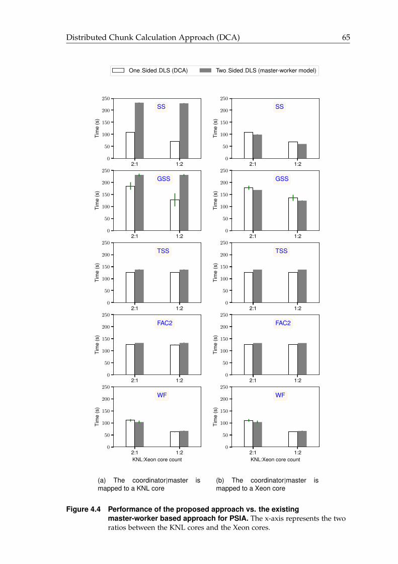
Distributed Chunk Calculation Approach (DCA) 65
2:1 1:20
20
40
60
80
Tim
e(s
)SS
One Sided DLS (DCA) Two Sided DLS (master-worker model)
2:1 1:20
20
40
60
80
Tim
e(s
)
GSS
2:1 1:20
20
40
60
80
Tim
e(s
)
TSS
2:1 1:20
20
40
60
80
Tim
e(s
)
FAC2
2:1 1:2KNL:Xeon core count
0
20
40
60
80
Tim
e(s
)
WF
2:1 1:20
50
100
150
200
250Ti
me
(s)
SS
2:1 1:20
50
100
150
200
250
Tim
e(s
)
GSS
2:1 1:20
50
100
150
200
250
Tim
e(s
)
TSS
2:1 1:20
50
100
150
200
250
Tim
e(s
)
FAC2
2:1 1:2KNL:Xeon core count
0
50
100
150
200
250
Tim
e(s
)
WF
(a) The coordinator|master ismapped to a KNL core
2:1 1:20
50
100
150
200
250
Tim
e(s
)
SS
2:1 1:20
50
100
150
200
250
Tim
e(s
)
GSS
2:1 1:20
50
100
150
200
250
Tim
e(s
)
TSS
2:1 1:20
50
100
150
200
250
Tim
e(s
)
FAC2
2:1 1:2KNL:Xeon core count
0
50
100
150
200
250
Tim
e(s
)
WF
(b) The coordinator|master ismapped to a Xeon core
Figure 4.4 Performance of the proposed approach vs. the existingmaster-worker based approach for PSIA. The x-axis represents the tworatios between the KNL cores and the Xeon cores.
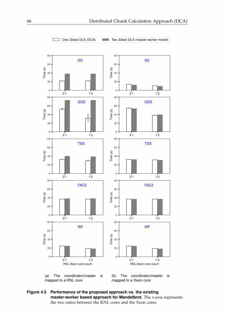
66 Distributed Chunk Calculation Approach (DCA)
2:1 1:20
20
40
60
80
Tim
e(s
)
SS
One Sided DLS (DCA) Two Sided DLS (master-worker model)
2:1 1:20
20
40
60
80
Tim
e(s
)
GSS
2:1 1:20
20
40
60
80
Tim
e(s
)
TSS
2:1 1:20
20
40
60
80
Tim
e(s
)
FAC2
2:1 1:2KNL:Xeon core count
0
20
40
60
80
Tim
e(s
)
WF
2:1 1:20
20
40
60
80
Tim
e(s
)
SS
2:1 1:20
20
40
60
80
Tim
e(s
)
GSS
2:1 1:20
20
40
60
80
Tim
e(s
)
TSS
2:1 1:20
20
40
60
80
Tim
e(s
)
FAC2
2:1 1:2KNL:Xeon core count
0
20
40
60
80
Tim
e(s
)
WF
(a) The coordinator|master ismapped to a KNL core
2:1 1:20
20
40
60
80
Tim
e(s
)
SS
2:1 1:20
20
40
60
80
Tim
e(s
)
GSS
2:1 1:20
20
40
60
80
Tim
e(s
)
TSS
2:1 1:20
20
40
60
80
Tim
e(s
)
FAC2
2:1 1:2KNL:Xeon core count
0
20
40
60
80
Tim
e(s
)
WF
(b) The coordinator|master ismapped to a Xeon core
Figure 4.5 Performance of the proposed approach vs. the existingmaster-worker based approach for Mandelbrot. The x-axis representsthe two ratios between the KNL cores and the Xeon cores.
Distributed Chunk Calculation Approach (DCA) 67
always prioritizes requests from the process with the smallest MPI rank. TheGSS has the largest non-linear decrement among the decrements of the selectedDLS techniques. Therefore, GSS is highly-sensitive to the chunk assignment.
Second observation: FAC2 and WF exhibit a reduced sensitivity to mappingthe master to a KNL or to a Xeon core. This low sensitivity could be due to thefactoring-based nature of these techniques. Among all the assessed DLS tech-niques, FAC2 and WF assign chunks in batches, which increases the possibilityfor the master to have chunks of the same size as the other processing elements.
4.5 Summary
The distributed chunk calculation approach (DCA) [EC19a] can be applied todifferent DLS techniques. DCA requires the mathematical chunk calculationformulas to be straightforward, i.e., they must only depend on constants andthe index of the last scheduling step i. Many DLS techniques have their math-ematical chunk calculation formulas in a recursive format, i.e., they depend onthe value of previously calculated chunk sizes [Luc92; TN93; CAB+01; PD97;Ban00]. However, we provided the mathematical transformations to changethese recursive formulas into straightforward formulas.
We implemented the proposed DCA using MPI RMA and passive targetsynchronization mode to exploit the latest advancements in the MPI standard(MPI 3.1). When the master was not mapped to the processing element withthe highest computing power, the results showed that the DLS techniques im-plemented with the proposed DCA outperformed their corresponding ones thatwere implemented with the conventional master-worker model execution model.When the master was mapped to the processing element with the highest com-puting power, the results showed that the DLS techniques implemented withthe proposed DCA performed competitively against their corresponding onesthat were implemented with the conventional master-worker model executionmodel. We conclude that the proposed DCA has a strong performance potentialfor irregular execution environment.

5Hierarchical Distributed ChunkCalculation Approach (HDCA)
As discussed in Chapter 4, DLS techniques typically employ a master-workerexecution model [CB05; BCP+05; CBR+04]. This model includes a processingentity called master. The master responsible for calculating and assigning chunksof loop iterations to all the other entities (workers). This model has scalinglimitations [CBR+04], and therefore, the DLS techniques have evolved to employa hierarchical master-worker execution model [CPY+05]. This model includestwo levels of masters: global and local masters. The global master calculatesand assigns chunks to local masters. Then, each of them becomes responsiblefor calculating and assigning sub-chunks to its group of workers. The globalmaster and local masters may exploit different DLS techniques. The use of DLStechniques at two levels is also referred to as a hierarchical DLS technique.
Hybrid MPI+OpenMP is a common programming approach to implementhierarchical DLS techniques. However, it has specific performance challenges,such as the added overhead for managing two levels of parallelism using twodifferent runtime systems. The OpenMP threads (workers) require synchro-nization before requesting and executing chunks, i.e., only the main thread isallowed to call MPI communication functions, such as MPI_Send and MPI_-Receive [WYL+12]. Otherwise, a complex implementation is needed to allowindividual OpenMP threads to perform MPI calls.
In this chapter, we propose a novel approach for designing and develop-ing hierarchical DLS techniques for distributed-memory systems. It extendsthe proposed DCA [EC19a] by allowing any group of workers that reside on ashared-memory system to form a shared work queue. The novelty of the pro-posed approach lies in the fact that the work queue’s responsibility is shared
70 Hierarchical Distributed Chunk Calculation Approach (HDCA)
among the workers of the group rather than one specific entity (local master).
We consider the shared-memory features offered in the MPI-3 standard. Thisfeature enables assigning chunks to individual MPI processes in two stages. Inthe first stage, the fastest MPI process within a compute node obtains a chunkbased on a selected DLS technique and then uses the obtained chunk to fill alocal shared queue. In the second stage, the MPI processes within the sameshared-memory system use a different or a similar DLS technique to obtainsub-chucks from the shared local work queue.
5.1 Hierarchical DLS Techniques
In the master-worker execution model, the number of requests that could be re-ceived by the master process is proportional to the total number of workers. Fora large number of workers, the master may simultaneously receive a large num-ber of work requests, and if the handling of the work requests is inefficient, themaster becomes a performance bottleneck. To overcome such limitation, certainresearch efforts proposed the use of the hierarchical master-worker approach.For instance, a distributed self-scheduling scheme (HDSS) using the hierarchi-cal master-worker model was introduced [CPY+05]. Unlike the LB-tool, HDSSdedicated the master process for handling the worker requests. The proposedscheme was implemented using MPI and its classical two-sided communication.
Another research effort discussed the adverse impact of the foreman-worker(master-worker) model [CBR+04] on DLS techniques. The authors suggesteda new execution model using processor groups. The idea was to form a fewgroups of processors, where each group executes a specified portion of the iter-ation space using the master-worker model. The master process of each grouphas to periodically update a global master process called manager. The mastersupdate the manager with the ratio of the remaining iterations and the availableworkers. When the reported ratio exceeds a certain threshold, the manager mi-grates workers between processor groups. Migrating workers to a certain groupmay result in a large number of workers within that group. This research ef-fort [CBR+04] is similar to our proposed HDCA [EC19b] as both balance theloop execution using two levels scheduling levels. However, the present workdiffers by exploiting different DLS techniques at the first level, while the sug-gested execution model in [CBR+04] statically divides the loop iteration spaceamong processor groups. Moreover, the present work avoids worker migrationthat may result in performance degradation when the cost of managing and
Hierarchical Distributed Chunk Calculation Approach (HDCA) 71
serving requests from the migrated workers becomes relatively large. The sug-gested execution model was implemented using MPI, and it did not take theadvantage of the shared-memory between processing elements.
Modern HPC systems are clusters of multi- and many-core systems con-nected via high-speed interconnection networks [CW10]. Developers often com-bine two different programming models to target such systems. A common ap-proach is to use MPI [For20] for inter-node communication and OpenMP [Boa18]for programming the shared-memory systems [SB01]. In the context of DLStechniques, the hierarchical loop scheduling (HLS) [WYL+12] was one of theearliest efforts to use the MPI+OpenMP programming model. In HLS, a freeworker (MPI process) requests a chunk from the master rank, which calculatesand assigns the chunk based on a certain performance function [SYT07]. Theworkers (MPI processes) locally use OpenMP loop scheduling techniques, suchas static, dynamic, and guided to execute the assigned chunk.
5.2 Maintaining Local Work Queues
The proposed approach applies two DLS techniques at the intra- and inter-nodelevels as follows. One MPI process creates a global shared-memory region calledthe global work queue. This global queue stores information regarding thelatest scheduling step and the total scheduled loop iterations [EC19a]. UsingMPI_Win_allocate_shared, the MPI processes within one compute node cre-ate another shared-memory region called the local work queue. This local queuestores information regarding the latest scheduling step and the total scheduledloop iterations by the MPI processes within that physical node. Whenever anMPI process becomes free, it obtains a sub-chunk from the local work queue. Ifthere are no sub-chunks, the MPI process tries to obtain a chunk from the globalwork queue and fills the empty local work queue. In the proposed HDCA, theMPI processes do not wait for each other to fill the local work queue. The re-sponsibility of obtaining work is not assigned to a specific MPI process, as thefastest MPI process always takes this responsibility. Figure 5.1 illustrates theproposed HDCA using the MPI shared memory feature, known as MPI+MPIapproach [HDB+13].
Unlike existing MPI+OpenMP implementations of DLS techniques, the pro-posed approach avoids the implicit synchronization that is required at the endchunks’ execution. Figure 5.2 illustrates the undesired implicit thread synchro-nization when using the MPI+OpenMP approach. OpenMP Thread 1 finished
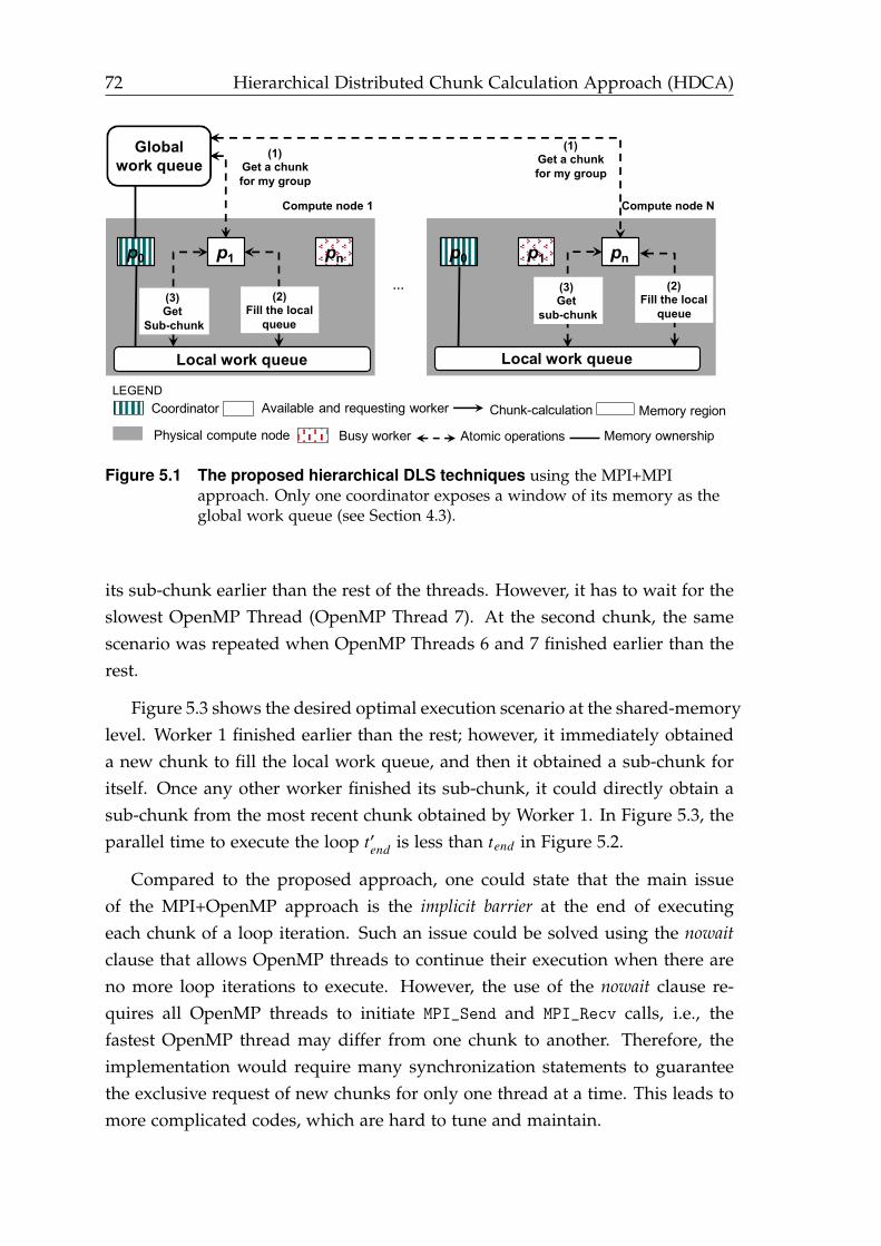
72 Hierarchical Distributed Chunk Calculation Approach (HDCA)
p0 pn…p0
Global work queue
Local work queue
p1
(2) Fill the local
queue
pn p1
(1) Get a chunk for my group
(3) Get
Sub-chunk
(1) Get a chunk for my group
(3) Get
sub-chunk
Local work queue
(2) Fill the local
queue
Compute node 1 Compute node N
…
LEGENDCoordinator
Busy worker Atomic operationsPhysical compute node
Chunk-calculationAvailable and requesting worker Memory region
Memory ownership
Figure 5.1 The proposed hierarchical DLS techniques using the MPI+MPIapproach. Only one coordinator exposes a window of its memory as theglobal work queue (see Section 4.3).
its sub-chunk earlier than the rest of the threads. However, it has to wait for theslowest OpenMP Thread (OpenMP Thread 7). At the second chunk, the samescenario was repeated when OpenMP Threads 6 and 7 finished earlier than therest.
Figure 5.3 shows the desired optimal execution scenario at the shared-memorylevel. Worker 1 finished earlier than the rest; however, it immediately obtaineda new chunk to fill the local work queue, and then it obtained a sub-chunk foritself. Once any other worker finished its sub-chunk, it could directly obtain asub-chunk from the most recent chunk obtained by Worker 1. In Figure 5.3, theparallel time to execute the loop t′end is less than tend in Figure 5.2.
Compared to the proposed approach, one could state that the main issueof the MPI+OpenMP approach is the implicit barrier at the end of executingeach chunk of a loop iteration. Such an issue could be solved using the nowaitclause that allows OpenMP threads to continue their execution when there areno more loop iterations to execute. However, the use of the nowait clause re-quires all OpenMP threads to initiate MPI_Send and MPI_Recv calls, i.e., thefastest OpenMP thread may differ from one chunk to another. Therefore, theimplementation would require many synchronization statements to guaranteethe exclusive request of new chunks for only one thread at a time. This leads tomore complicated codes, which are hard to tune and maintain.
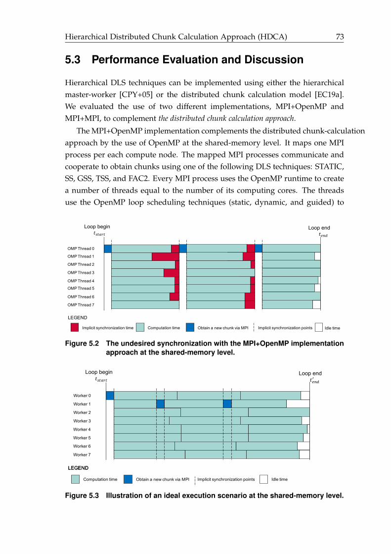
Hierarchical Distributed Chunk Calculation Approach (HDCA) 73
5.3 Performance Evaluation and Discussion
Hierarchical DLS techniques can be implemented using either the hierarchicalmaster-worker [CPY+05] or the distributed chunk calculation model [EC19a].We evaluated the use of two different implementations, MPI+OpenMP andMPI+MPI, to complement the distributed chunk calculation approach.
The MPI+OpenMP implementation complements the distributed chunk-calculationapproach by the use of OpenMP at the shared-memory level. It maps one MPIprocess per each compute node. The mapped MPI processes communicate andcooperate to obtain chunks using one of the following DLS techniques: STATIC,SS, GSS, TSS, and FAC2. Every MPI process uses the OpenMP runtime to createa number of threads equal to the number of its computing cores. The threadsuse the OpenMP loop scheduling techniques (static, dynamic, and guided) to
Idle time
OMP Thread 0
OMP Thread 1
OMP Thread 2
OMP Thread 3
OMP Thread 4
OMP Thread 5
OMP Thread 6
OMP Thread 7
LEGEND
Implicit synchronization time Computation time Obtain a new chunk via MPI
Loop begin𝑡"#$%#
Loop end𝑡&'(
Implicit synchronization points
Figure 5.2 The undesired synchronization with the MPI+OpenMP implementationapproach at the shared-memory level.
Worker 0
Worker 1
Worker 2
Worker 3
Worker 4
Worker 5
Worker 6
Worker 7
Loop begin𝑡"#$%#
Loop end𝑡&'()
LEGENDLEGEND
Computation time Obtain a new chunk via MPI Implicit synchronization points Idle time
Figure 5.3 Illustration of an ideal execution scenario at the shared-memory level.
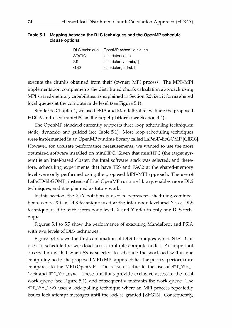
74 Hierarchical Distributed Chunk Calculation Approach (HDCA)
Table 5.1 Mapping between the DLS techniques and the OpenMP scheduleclause options
DLS technique OpenMP schedule clauseSTATIC schedule(static)SS schedule(dynamic,1)GSS schedule(guided,1)
execute the chunks obtained from their (owner) MPI process. The MPI+MPIimplementation complements the distributed chunk calculation approach usingMPI shared-memory capabilities, as explained in Section 5.2, i.e., it forms sharedlocal queues at the compute node level (see Figure 5.1).
Similar to Chapter 4, we used PSIA and Mandelbrot to evaluate the proposedHDCA and used miniHPC as the target platform (see Section 4.4).
The OpenMP standard currently supports three loop scheduling techniques:static, dynamic, and guided (see Table 5.1). More loop scheduling techniqueswere implemented in an OpenMP runtime library called LaPeSD-libGOMP [CIB18].However, for accurate performance measurements, we wanted to use the mostoptimized software installed on miniHPC. Given that miniHPC (the target sys-tem) is an Intel-based cluster, the Intel software stack was selected, and there-fore, scheduling experiments that have TSS and FAC2 at the shared-memorylevel were only performed using the proposed MPI+MPI approach. The use ofLaPeSD-libGOMP, instead of Intel OpenMP runtime library, enables more DLStechniques, and it is planned as future work.
In this section, the X+Y notation is used to represent scheduling combina-tions, where X is a DLS technique used at the inter-node level and Y is a DLStechnique used to at the intra-node level. X and Y refer to only one DLS tech-nique.
Figures 5.4 to 5.7 show the performance of executing Mandelbrot and PSIAwith two levels of DLS techniques.
Figure 5.4 shows the first combination of DLS techniques where STATIC isused to schedule the workload across multiple compute nodes. An importantobservation is that when SS is selected to schedule the workload within onecomputing node, the proposed MPI+MPI approach has the poorest performancecompared to the MPI+OpenMP. The reason is due to the use of MPI_Win_-
lock and MPI_Win_sync. These functions provide exclusive access to the localwork queue (see Figure 5.1), and consequently, maintain the work queue. TheMPI_Win_lock uses a lock polling technique where an MPI process repeatedlyissues lock-attempt messages until the lock is granted [ZBG16]. Consequently,
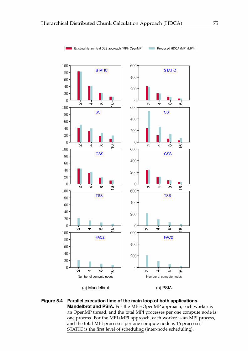
Hierarchical Distributed Chunk Calculation Approach (HDCA) 75
2 4 8 16
0
200
400
600Ti
me
(s)
STATIC
Existing hierarchical DLS approach (MPI+OpenMP) Proposed HDCA (MPI+MPI)
2 4 8 16
0
200
400
600
Tim
e(s
)
SS2 4 8 16
0
200
400
600
Tim
e(s
)
GSS
2 4 8 16
0
200
400
600
Tim
e(s
)
TSS
2 4 8 16
Number of compute nodes
0
200
400
600
Tim
e(s
)
FAC2
2 4 8 16
0
20
40
60
80
100
Tim
e(s
)
STATIC
2 4 8 16
0
20
40
60
80
100
Tim
e(s
)
SS
2 4 8 16
0
20
40
60
80
100
Tim
e(s
)
GSS
2 4 8 16
0
20
40
60
80
100
Tim
e(s
)
TSS
2 4 8 16
Number of compute nodes
0
20
40
60
80
100
Tim
e(s
)
FAC2
(a) Mandelbrot
2 4 8 16
0
200
400
600
Tim
e(s
)
STATIC
2 4 8 16
0
200
400
600
Tim
e(s
)
SS
2 4 8 160
200
400
600
Tim
e(s
)
GSS
2 4 8 16
0
200
400
600
Tim
e(s
)
TSS
2 4 8 16
Number of compute nodes
0
200
400
600
Tim
e(s
)
FAC2
(b) PSIA
Figure 5.4 Parallel execution time of the main loop of both applications,Mandelbrot and PSIA. For the MPI+OpenMP approach, each worker isan OpenMP thread, and the total MPI processes per one compute node isone process. For the MPI+MPI approach, each worker is an MPI process,and the total MPI processes per one compute node is 16 processes.STATIC is the first level of scheduling (inter-node scheduling).
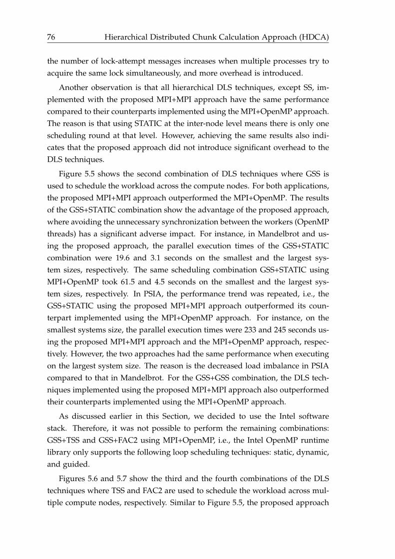
76 Hierarchical Distributed Chunk Calculation Approach (HDCA)
the number of lock-attempt messages increases when multiple processes try toacquire the same lock simultaneously, and more overhead is introduced.
Another observation is that all hierarchical DLS techniques, except SS, im-plemented with the proposed MPI+MPI approach have the same performancecompared to their counterparts implemented using the MPI+OpenMP approach.The reason is that using STATIC at the inter-node level means there is only onescheduling round at that level. However, achieving the same results also indi-cates that the proposed approach did not introduce significant overhead to theDLS techniques.
Figure 5.5 shows the second combination of DLS techniques where GSS isused to schedule the workload across the compute nodes. For both applications,the proposed MPI+MPI approach outperformed the MPI+OpenMP. The resultsof the GSS+STATIC combination show the advantage of the proposed approach,where avoiding the unnecessary synchronization between the workers (OpenMPthreads) has a significant adverse impact. For instance, in Mandelbrot and us-ing the proposed approach, the parallel execution times of the GSS+STATICcombination were 19.6 and 3.1 seconds on the smallest and the largest sys-tem sizes, respectively. The same scheduling combination GSS+STATIC usingMPI+OpenMP took 61.5 and 4.5 seconds on the smallest and the largest sys-tem sizes, respectively. In PSIA, the performance trend was repeated, i.e., theGSS+STATIC using the proposed MPI+MPI approach outperformed its coun-terpart implemented using the MPI+OpenMP approach. For instance, on thesmallest systems size, the parallel execution times were 233 and 245 seconds us-ing the proposed MPI+MPI approach and the MPI+OpenMP approach, respec-tively. However, the two approaches had the same performance when executingon the largest system size. The reason is the decreased load imbalance in PSIAcompared to that in Mandelbrot. For the GSS+GSS combination, the DLS tech-niques implemented using the proposed MPI+MPI approach also outperformedtheir counterparts implemented using the MPI+OpenMP approach.
As discussed earlier in this Section, we decided to use the Intel softwarestack. Therefore, it was not possible to perform the remaining combinations:GSS+TSS and GSS+FAC2 using MPI+OpenMP, i.e., the Intel OpenMP runtimelibrary only supports the following loop scheduling techniques: static, dynamic,and guided.
Figures 5.6 and 5.7 show the third and the fourth combinations of the DLStechniques where TSS and FAC2 are used to schedule the workload across mul-tiple compute nodes, respectively. Similar to Figure 5.5, the proposed approach
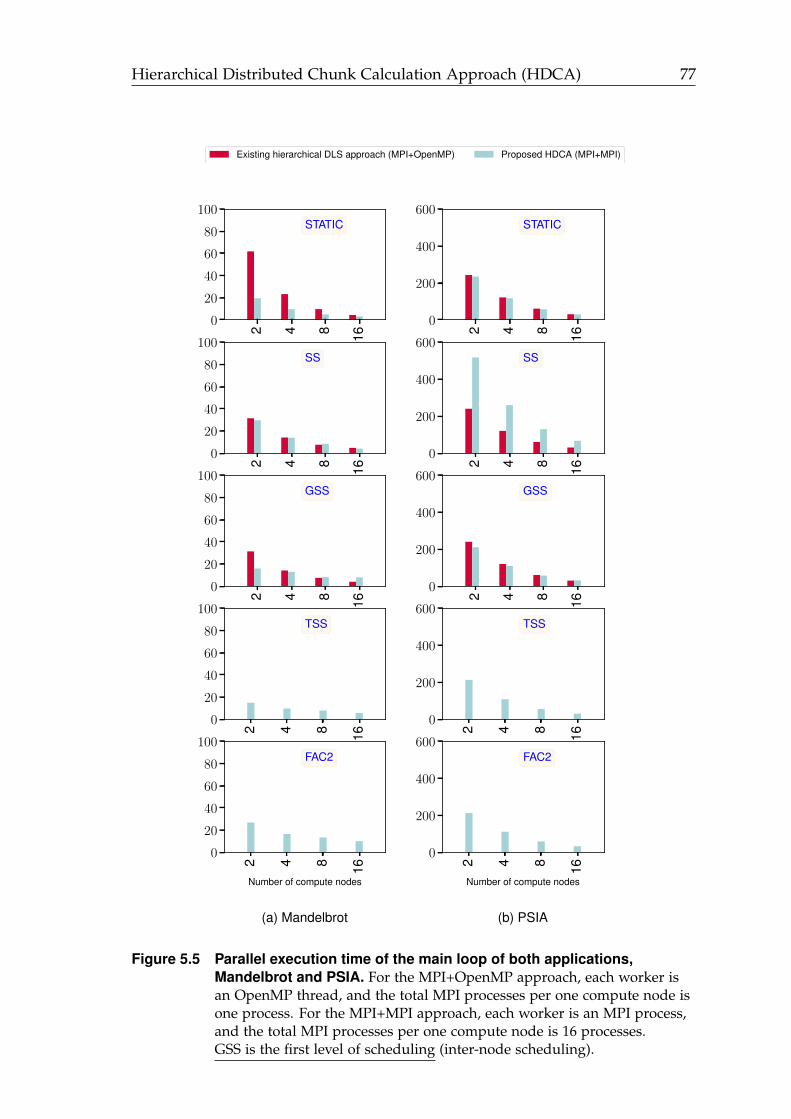
Hierarchical Distributed Chunk Calculation Approach (HDCA) 77
2 4 8 16
0
200
400
600Ti
me
(s)
STATIC
Existing hierarchical DLS approach (MPI+OpenMP) Proposed HDCA (MPI+MPI)
2 4 8 16
0
200
400
600
Tim
e(s
)
SS2 4 8 16
0
200
400
600
Tim
e(s
)
GSS
2 4 8 16
0
200
400
600
Tim
e(s
)
TSS
2 4 8 16
Number of compute nodes
0
200
400
600
Tim
e(s
)
FAC2
2 4 8 16
0
20
40
60
80
100
Tim
e(s
)
STATIC
2 4 8 16
0
20
40
60
80
100
Tim
e(s
)
SS
2 4 8 16
0
20
40
60
80
100
Tim
e(s
)
GSS
2 4 8 16
0
20
40
60
80
100
Tim
e(s
)
TSS
2 4 8 16
Number of compute nodes
0
20
40
60
80
100
Tim
e(s
)
FAC2
(a) Mandelbrot
2 4 8 16
0
200
400
600
Tim
e(s
)
STATIC
2 4 8 16
0
200
400
600
Tim
e(s
)
SS
2 4 8 160
200
400
600
Tim
e(s
)
GSS
2 4 8 16
0
200
400
600
Tim
e(s
)
TSS
2 4 8 16
Number of compute nodes
0
200
400
600
Tim
e(s
)
FAC2
(b) PSIA
Figure 5.5 Parallel execution time of the main loop of both applications,Mandelbrot and PSIA. For the MPI+OpenMP approach, each worker isan OpenMP thread, and the total MPI processes per one compute node isone process. For the MPI+MPI approach, each worker is an MPI process,and the total MPI processes per one compute node is 16 processes.GSS is the first level of scheduling (inter-node scheduling).
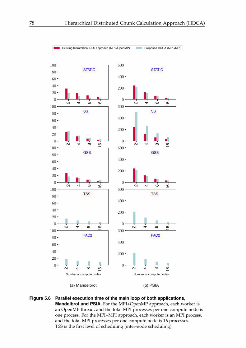
78 Hierarchical Distributed Chunk Calculation Approach (HDCA)
2 4 8 16
0
200
400
600
Tim
e(s
)
STATIC
Existing hierarchical DLS approach (MPI+OpenMP) Proposed HDCA (MPI+MPI)
2 4 8 16
0
200
400
600
Tim
e(s
)
SS
2 4 8 16
0
200
400
600
Tim
e(s
)
GSS
2 4 8 160
200
400
600
Tim
e(s
)
TSS
2 4 8 16
Number of compute nodes
0
200
400
600
Tim
e(s
)
FAC2
2 4 8 160
20
40
60
80
100
Tim
e(s
)
STATIC2 4 8 16
0
20
40
60
80
100
Tim
e(s
)
SS
2 4 8 16
0
20
40
60
80
100
Tim
e(s
)
GSS
2 4 8 16
0
20
40
60
80
100
Tim
e(s
)
TSS
2 4 8 16
Number of compute nodes
0
20
40
60
80
100
Tim
e(s
)
FAC2
(a) Mandelbrot
2 4 8 16
0
200
400
600
Tim
e(s
)
STATIC
2 4 8 16
0
200
400
600
Tim
e(s
)SS
2 4 8 16
0
200
400
600
Tim
e(s
)
GSS
2 4 8 16
0
200
400
600
Tim
e(s
)
TSS
2 4 8 16
Number of compute nodes
0
200
400
600
Tim
e(s
)
FAC2
(b) PSIA
Figure 5.6 Parallel execution time of the main loop of both applications,Mandelbrot and PSIA. For the MPI+OpenMP approach, each worker isan OpenMP thread, and the total MPI processes per one compute node isone process. For the MPI+MPI approach, each worker is an MPI process,and the total MPI processes per one compute node is 16 processes.TSS is the first level of scheduling (inter-node scheduling).
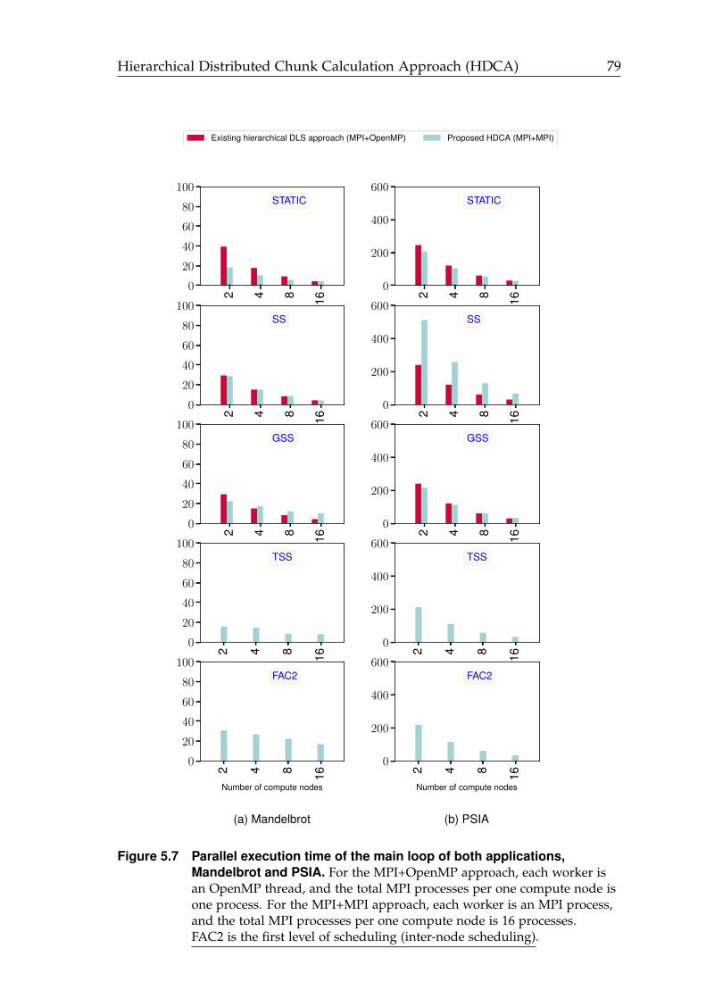
Hierarchical Distributed Chunk Calculation Approach (HDCA) 79
2 4 8 16
0
200
400
600Ti
me
(s)
STATIC
Existing hierarchical DLS approach (MPI+OpenMP) Proposed HDCA (MPI+MPI)
2 4 8 16
0
200
400
600
Tim
e(s
)
SS2 4 8 16
0
200
400
600
Tim
e(s
)
GSS
2 4 8 16
0
200
400
600
Tim
e(s
)
TSS
2 4 8 16
Number of compute nodes
0
200
400
600
Tim
e(s
)
FAC2
2 4 8 16
0
20
40
60
80
100
Tim
e(s
)
STATIC
2 4 8 16
0
20
40
60
80
100
Tim
e(s
)
SS
2 4 8 16
0
20
40
60
80
100
Tim
e(s
)
GSS
2 4 8 16
0
20
40
60
80
100
Tim
e(s
)
TSS
2 4 8 16
Number of compute nodes
0
20
40
60
80
100
Tim
e(s
)
FAC2
(a) Mandelbrot
2 4 8 16
0
200
400
600
Tim
e(s
)
STATIC
2 4 8 16
0
200
400
600
Tim
e(s
)
SS
2 4 8 160
200
400
600
Tim
e(s
)
GSS
2 4 8 16
0
200
400
600
Tim
e(s
)
TSS
2 4 8 16
Number of compute nodes
0
200
400
600
Tim
e(s
)
FAC2
(b) PSIA
Figure 5.7 Parallel execution time of the main loop of both applications,Mandelbrot and PSIA. For the MPI+OpenMP approach, each worker isan OpenMP thread, and the total MPI processes per one compute node isone process. For the MPI+MPI approach, each worker is an MPI process,and the total MPI processes per one compute node is 16 processes.FAC2 is the first level of scheduling (inter-node scheduling).
80 Hierarchical Distributed Chunk Calculation Approach (HDCA)
significantly outperformed the MPI+OpenMP approach when STATIC is se-lected for scheduling the computational workload within one compute node.For the rest of the scheduling combinations, both approaches have the sameperformance. The only exception is when applying SS at the shared-memorylevel. The proposed approach has the worst performance compared to theMPI+OpenMP approach. The reason is that SS achieves the maximum load bal-ance, and most of the workers (OpenMP threads) finish at the same time. Thisscenario will avoid the long synchronization time before getting new chunks.
The last observation is related to the performance of the PSIA when applyingany combination that has the SS using the proposed approach. PSIA has lessload imbalance than Mandelbrot, and the proposed approach has a significantoverhead when employing SS. Consequently, the adverse impact of the largeassociated scheduling overhead of SS is more visible in PSIA than Mandelbrot.
5.4 Summary
The implementation of hierarchical DLS techniques is essential to enable scal-able application performance. Because of the centralized work queue (loop it-erations), efficient implementations of hierarchical DLS techniques may be bet-ter than non-hierarchical ones. When STATIC is used for the intra-node levelscheduling, the proposed HDCA that employs the MPI+MPI approach outper-formed the one that uses the hybrid MPI+OpenMP approach. This highlightsand confirms the capability of our proposed HDCA to eliminate the unrequiredsynchronization at the intra-node level. On the contrary, the MPI+MPI ap-proach shows a limited performance when many MPI processes on the sameshared-memory system try to access the local work queue simultaneously. Theimportant observation of the present work is that the scheduling overhead asso-ciated with using MPI shared-memory to implement DLS techniques is higherthan OpenMP. Therefore, the use of the MPI+MPI approach is only recom-mended for developing hierarchical DLS techniques when its associated over-head is less than the synchronization overhead associated with the use of OpenMP.
6Resourceful Coordination Approach(RCA) for Multilevel Scheduling
The multilevel Scheduling (MLS) refers to exchanging scheduling informationbetween all scheduling levels, such as batch, application, and thread level. MLShelps to refine scheduling decisions at a certain level based on the availableinformation regarding the current scheduling workload at other levels. We pro-pose a resourceful coordination approach (RCA) that enables the cooperationbetween, currently independent, batch- and application-level schedulers. RCAenables application schedulers to share their allocated but idle computing re-sources with other applications through the batch system. With enabling thiscoordination, RCA avoids resource shrinking operations and associated perfor-mance penalties that are typical of dynamic resource and job management sys-tems. To evaluate RCA, we bridged a Slurm-based simulator(at the batch-level)and a SimGrid-based simulator flowing the same principle of the two-level sim-ulation approach that we presented in Chapter 3.
6.1 Coordination Between ALS and BLS
The resourceful coordination approach (RCA) requires information exchangebetween batch and application schedulers: (1) From the application schedulersto the batch scheduler. The application schedulers report the status of their freecomputing resources and the remaining amount of work. (2) From the batchscheduler to the application schedulers. The batch scheduler can take advantageof knowing the execution history of certain applications and can benefit fromadditional hints that the user may provide, such as expected applications’ exe-
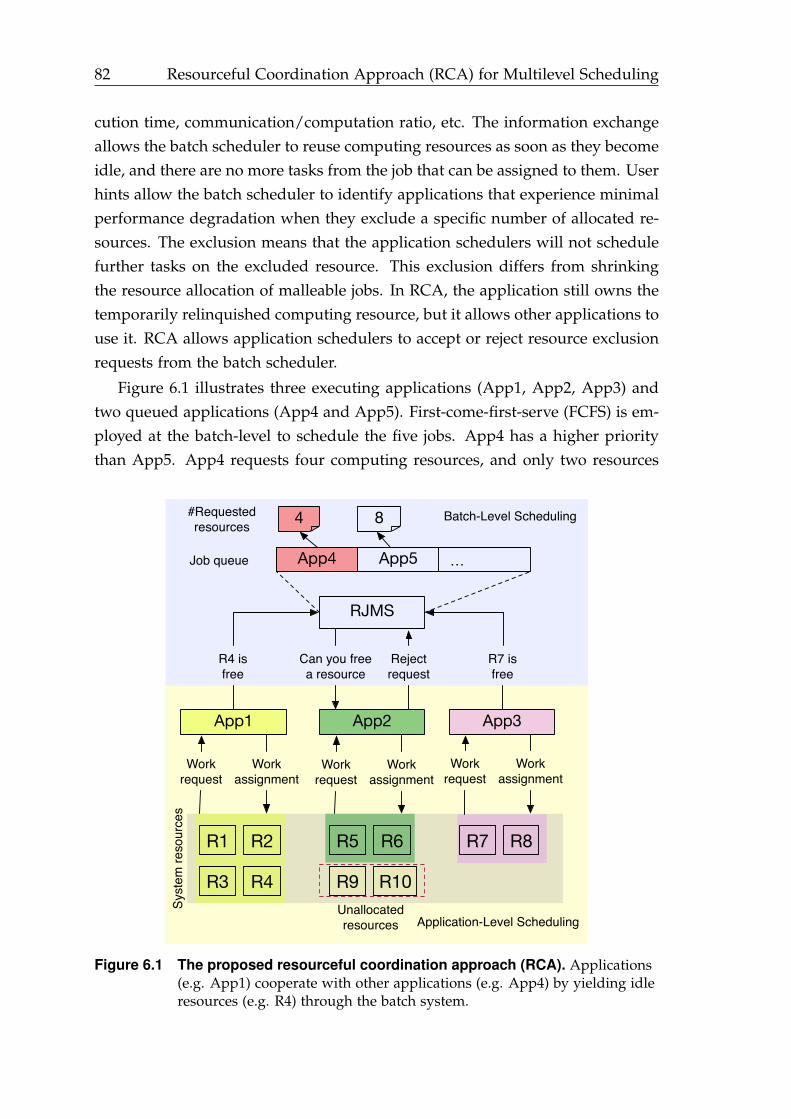
82 Resourceful Coordination Approach (RCA) for Multilevel Scheduling
cution time, communication/computation ratio, etc. The information exchangeallows the batch scheduler to reuse computing resources as soon as they becomeidle, and there are no more tasks from the job that can be assigned to them. Userhints allow the batch scheduler to identify applications that experience minimalperformance degradation when they exclude a specific number of allocated re-sources. The exclusion means that the application schedulers will not schedulefurther tasks on the excluded resource. This exclusion differs from shrinkingthe resource allocation of malleable jobs. In RCA, the application still owns thetemporarily relinquished computing resource, but it allows other applications touse it. RCA allows application schedulers to accept or reject resource exclusionrequests from the batch scheduler.
Figure 6.1 illustrates three executing applications (App1, App2, App3) andtwo queued applications (App4 and App5). First-come-first-serve (FCFS) is em-ployed at the batch-level to schedule the five jobs. App4 has a higher prioritythan App5. App4 requests four computing resources, and only two resources
App4Job queue App5 …
#Requestedresources 4 8
App1
R1 R2
R3 R4
App2 App3
R5 R6 R7 R8
R9 R10
Syst
em re
sour
ces
R4 is free
Rejectrequest
RJMS
R7 is free
Unallocated resources
Workrequest
Workassignment
Batch-Level Scheduling
Application-Level Scheduling
Can you freea resource
Workrequest
Workassignment
Workrequest
Workassignment
Figure 6.1 The proposed resourceful coordination approach (RCA). Applications(e.g. App1) cooperate with other applications (e.g. App4) by yielding idleresources (e.g. R4) through the batch system.
Resourceful Coordination Approach (RCA) for Multilevel Scheduling 83
are available: R9 and R10. However, the batch system cannot start App4 dueto insufficient free resources. Assuming that BF [FW98] is enabled, the batchsystem launches any job from the queue that requests at most two resources.In the example, App5 requests eight resources, and no other applications ex-ist in the queue. Existing batch scheduling systems would leave App4 waitingin the queue and R9 and R10 idle until one of the executing applications fin-ish. In contrast, in RCA, the batch system receives information form applicationschedulers during applications’ execution. App1 and App3 report that R4 andR7 became free. R4 and R7 can be reassigned to other applications through thebatch system. The information from App1 and App3 may be reported at differ-ent times. Once the batch system receives these two reports, and if App4 is stillin the queue, the batch system can assign R4, R9, R10, and R7 to App4, whichcan then begin execution.
The batch system can identify (based on applications’ execution history) ap-plications that can relinquish specific resources without performance degrada-tion. In the example illustrated in Figure 6.1, the batch system identified App2as such an application. The application scheduler of App2 rejected the requestand did not release any resources. In RCA, the batch scheduler does not con-trol the ALS decisions. Application schedulers can reject the release of resourcerequests. Accepting or rejecting batch requests can be seen as a higher level ofcooperation than reporting resource idle time that can be enabled or disabledbased on users’ preferences. Moreover, the batch system leaves the decision re-garding which resource to be freed to the application scheduler. RCA aims toseparate the concerns between BLS and ALS. BLS tries to provide the requirednumber of resources to waiting jobs, while ALS decides which resource(s) is(are) ready to be released right away.
6.2 RCA Applied to a BLS Simulator and an ALSSimulator
Design details: At batch-level scheduling, the current work employs the widelyused Slurm simulator [Luc11]. The current work extends and modifies one ofthe latest versions of the Slurm simulator [SDI+18]. Listing 6.1 shows the modi-fications required to support RCA.
In Algorithm 6.1, Line 2 shows the new code that has been added to al-low the Slurm simulator to read ALS information, such as the ALS schedulingmethod. Line 3 represents the modified code that extends the Slurm simula-
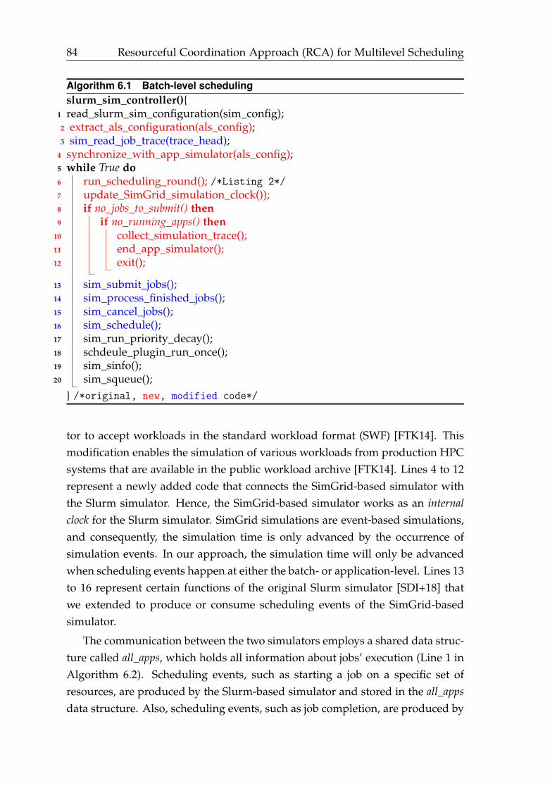
84 Resourceful Coordination Approach (RCA) for Multilevel Scheduling
Algorithm 6.1 Batch-level schedulingslurm_sim_controller(){
1 read_slurm_sim_configuration(sim_config);2 extract_als_configuration(als_config);3 sim_read_job_trace(trace_head);
4 synchronize_with_app_simulator(als_config);5 while True do6 run_scheduling_round(); /*Listing 2*/7 update_SimGrid_simulation_clock());8 if no_jobs_to_submit() then9 if no_running_apps() then
10 collect_simulation_trace();11 end_app_simulator();12 exit();
13 sim_submit_jobs();14 sim_process_finished_jobs();15 sim_cancel_jobs();16 sim_schedule();17 sim_run_priority_decay();18 schdeule_plugin_run_once();19 sim_sinfo();20 sim_squeue();
} /*original, new, modified code*/
tor to accept workloads in the standard workload format (SWF) [FTK14]. Thismodification enables the simulation of various workloads from production HPCsystems that are available in the public workload archive [FTK14]. Lines 4 to 12represent a newly added code that connects the SimGrid-based simulator withthe Slurm simulator. Hence, the SimGrid-based simulator works as an internalclock for the Slurm simulator. SimGrid simulations are event-based simulations,and consequently, the simulation time is only advanced by the occurrence ofsimulation events. In our approach, the simulation time will only be advancedwhen scheduling events happen at either the batch- or application-level. Lines 13to 16 represent certain functions of the original Slurm simulator [SDI+18] thatwe extended to produce or consume scheduling events of the SimGrid-basedsimulator.
The communication between the two simulators employs a shared data struc-ture called all_apps, which holds all information about jobs’ execution (Line 1 inAlgorithm 6.2). Scheduling events, such as starting a job on a specific set ofresources, are produced by the Slurm-based simulator and stored in the all_appsdata structure. Also, scheduling events, such as job completion, are produced by
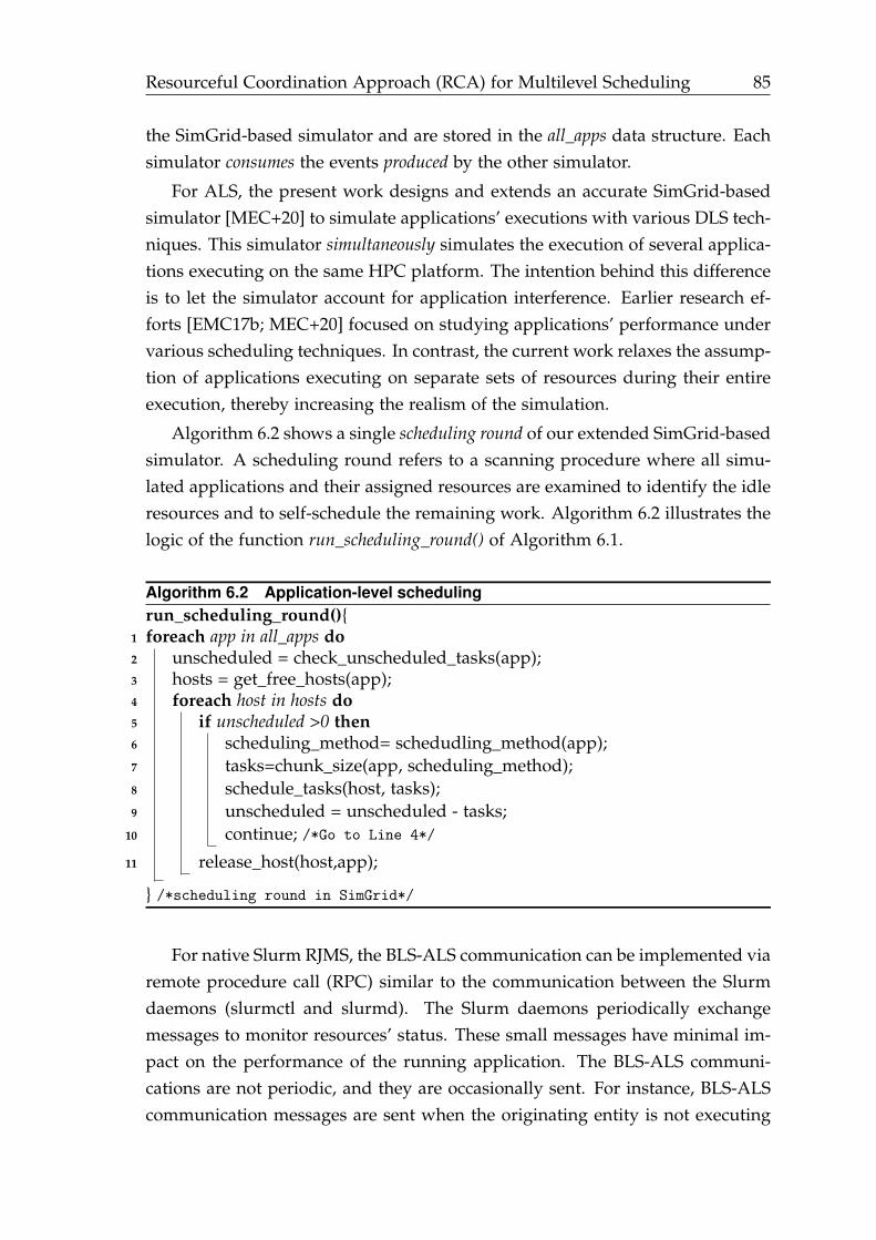
Resourceful Coordination Approach (RCA) for Multilevel Scheduling 85
the SimGrid-based simulator and are stored in the all_apps data structure. Eachsimulator consumes the events produced by the other simulator.
For ALS, the present work designs and extends an accurate SimGrid-basedsimulator [MEC+20] to simulate applications’ executions with various DLS tech-niques. This simulator simultaneously simulates the execution of several applica-tions executing on the same HPC platform. The intention behind this differenceis to let the simulator account for application interference. Earlier research ef-forts [EMC17b; MEC+20] focused on studying applications’ performance undervarious scheduling techniques. In contrast, the current work relaxes the assump-tion of applications executing on separate sets of resources during their entireexecution, thereby increasing the realism of the simulation.
Algorithm 6.2 shows a single scheduling round of our extended SimGrid-basedsimulator. A scheduling round refers to a scanning procedure where all simu-lated applications and their assigned resources are examined to identify the idleresources and to self-schedule the remaining work. Algorithm 6.2 illustrates thelogic of the function run_scheduling_round() of Algorithm 6.1.
Algorithm 6.2 Application-level schedulingrun_scheduling_round(){
1 foreach app in all_apps do2 unscheduled = check_unscheduled_tasks(app);3 hosts = get_free_hosts(app);4 foreach host in hosts do5 if unscheduled >0 then6 scheduling_method= schedudling_method(app);7 tasks=chunk_size(app, scheduling_method);8 schedule_tasks(host, tasks);9 unscheduled = unscheduled - tasks;
10 continue; /*Go to Line 4*/
11 release_host(host,app);
} /*scheduling round in SimGrid*/
For native Slurm RJMS, the BLS-ALS communication can be implemented viaremote procedure call (RPC) similar to the communication between the Slurmdaemons (slurmctl and slurmd). The Slurm daemons periodically exchangemessages to monitor resources’ status. These small messages have minimal im-pact on the performance of the running application. The BLS-ALS communi-cations are not periodic, and they are occasionally sent. For instance, BLS-ALScommunication messages are sent when the originating entity is not executing
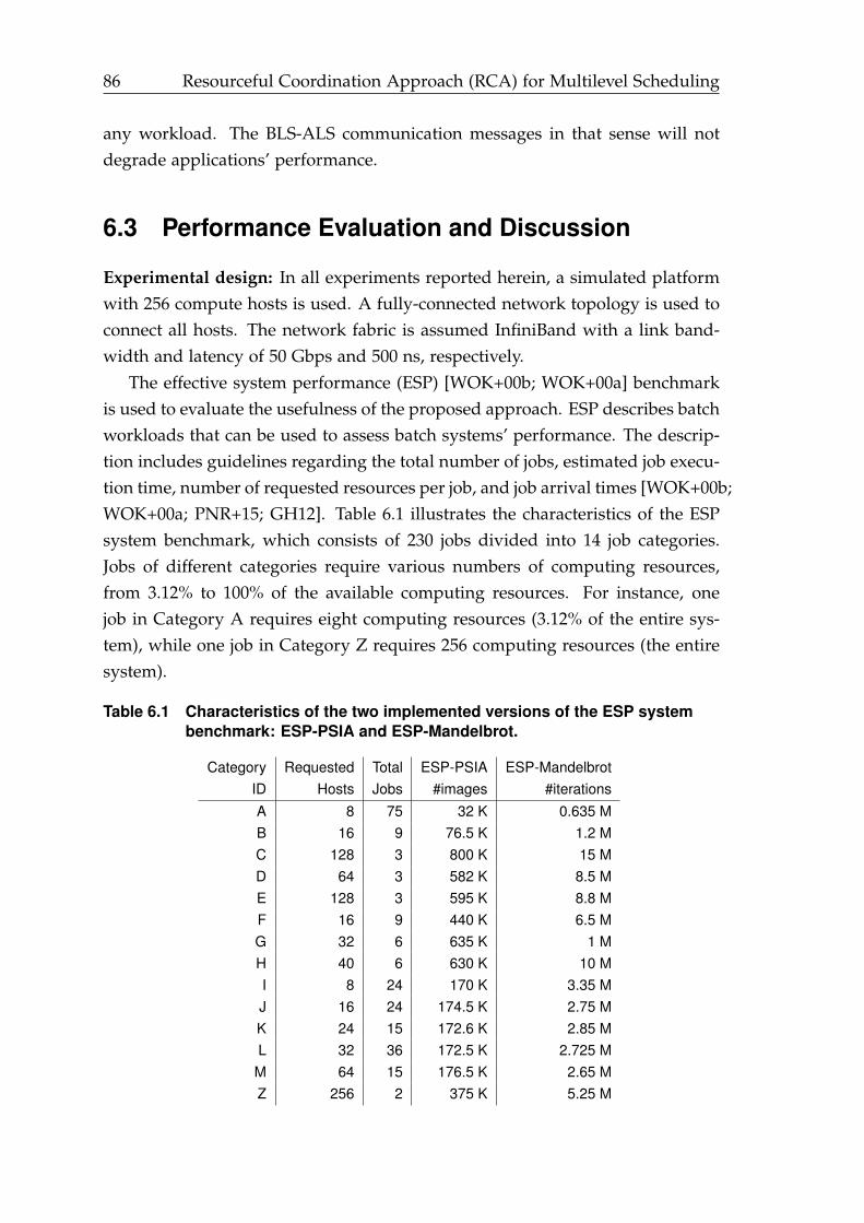
86 Resourceful Coordination Approach (RCA) for Multilevel Scheduling
any workload. The BLS-ALS communication messages in that sense will notdegrade applications’ performance.
6.3 Performance Evaluation and Discussion
Experimental design: In all experiments reported herein, a simulated platformwith 256 compute hosts is used. A fully-connected network topology is used toconnect all hosts. The network fabric is assumed InfiniBand with a link band-width and latency of 50 Gbps and 500 ns, respectively.
The effective system performance (ESP) [WOK+00b; WOK+00a] benchmarkis used to evaluate the usefulness of the proposed approach. ESP describes batchworkloads that can be used to assess batch systems’ performance. The descrip-tion includes guidelines regarding the total number of jobs, estimated job execu-tion time, number of requested resources per job, and job arrival times [WOK+00b;WOK+00a; PNR+15; GH12]. Table 6.1 illustrates the characteristics of the ESPsystem benchmark, which consists of 230 jobs divided into 14 job categories.Jobs of different categories require various numbers of computing resources,from 3.12% to 100% of the available computing resources. For instance, onejob in Category A requires eight computing resources (3.12% of the entire sys-tem), while one job in Category Z requires 256 computing resources (the entiresystem).
Table 6.1 Characteristics of the two implemented versions of the ESP systembenchmark: ESP-PSIA and ESP-Mandelbrot.
CategoryID
RequestedHosts
TotalJobs
ESP-PSIA#images
ESP-Mandelbrot#iterations
A 8 75 32 K 0.635 MB 16 9 76.5 K 1.2 MC 128 3 800 K 15 MD 64 3 582 K 8.5 ME 128 3 595 K 8.8 MF 16 9 440 K 6.5 MG 32 6 635 K 1 MH 40 6 630 K 10 MI 8 24 170 K 3.35 MJ 16 24 174.5 K 2.75 MK 24 15 172.6 K 2.85 ML 32 36 172.5 K 2.725 MM 64 15 176.5 K 2.65 MZ 256 2 375 K 5.25 M
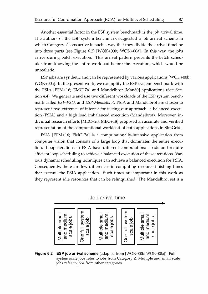
Resourceful Coordination Approach (RCA) for Multilevel Scheduling 87
Another essential factor in the ESP system benchmark is the job arrival time.The authors of the ESP system benchmark suggested a job arrival scheme inwhich Category Z jobs arrive in such a way that they divide the arrival timelineinto three parts (see Figure 6.2) [WOK+00b; WOK+00a]. In this way, the jobsarrive during batch execution. This arrival pattern prevents the batch sched-uler from knowing the entire workload before the execution, which would beunrealistic.
ESP jobs are synthetic and can be represented by various applications [WOK+00b;WOK+00a]. In the present work, we exemplify the ESP system benchmark withthe PSIA [EFM+16; EMC17a] and Mandelbrot [Man80] applications (See Sec-tion 4.4). We generate and use two different workloads of the ESP system bench-mark called ESP-PSIA and ESP-Mandelbrot. PSIA and Mandelbrot are chosen torepresent two extremes of interest for testing our approach: a balanced execu-tion (PSIA) and a high load imbalanced execution (Mandelbrot). Moreover, in-dividual research efforts [MEC+20; MEC+18] proposed an accurate and verifiedrepresentation of the computational workload of both applications in SimGrid.
PSIA [EFM+16; EMC17a] is a computationally-intensive application fromcomputer vision that consists of a large loop that dominates the entire execu-tion. Loop iterations in PSIA have different computational loads and requireefficient loop scheduling to achieve a balanced execution of these iterations. Var-ious dynamic scheduling techniques can achieve a balanced execution for PSIA.Consequently, there are few differences in computing resource finishing timesthat execute the PSIA application. Such times are important in this work asthey represent idle resources that can be relinquished. The Mandelbrot set is a
Mul
tiple
sm
all
and
med
ium
sc
ale
jobs
One
full
syst
em
scal
e jo
b
Job arrival time
Mul
tiple
sm
all
and
med
ium
sc
ale
jobs
One
full
syst
em
scal
e jo
b
Mul
tiple
sm
all
and
med
ium
sc
ale
jobs
Figure 6.2 ESP job arrival scheme (adapted from [WOK+00b; WOK+00a]). Fullsystem scale jobs refer to jobs from Category Z. Multiple and small scalejobs refer to jobs from other categories.
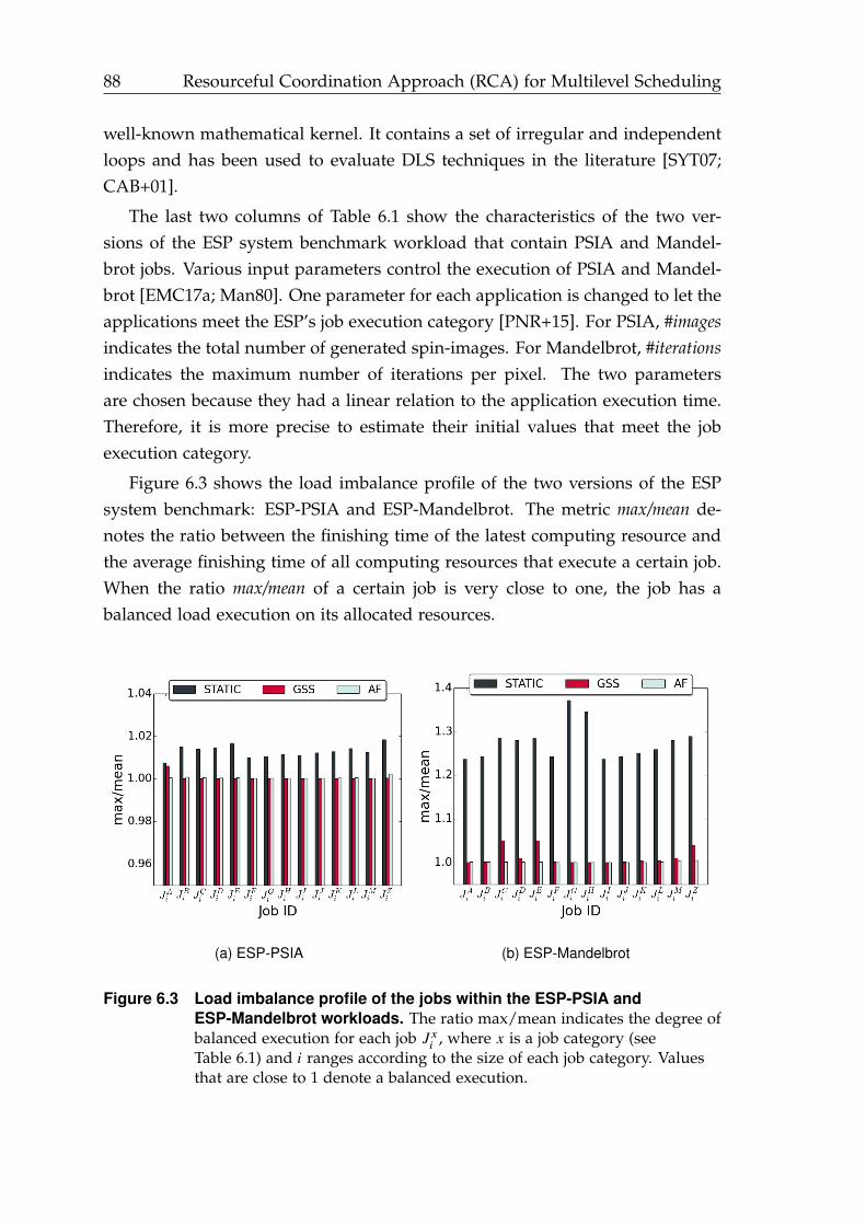
88 Resourceful Coordination Approach (RCA) for Multilevel Scheduling
well-known mathematical kernel. It contains a set of irregular and independentloops and has been used to evaluate DLS techniques in the literature [SYT07;CAB+01].
The last two columns of Table 6.1 show the characteristics of the two ver-sions of the ESP system benchmark workload that contain PSIA and Mandel-brot jobs. Various input parameters control the execution of PSIA and Mandel-brot [EMC17a; Man80]. One parameter for each application is changed to let theapplications meet the ESP’s job execution category [PNR+15]. For PSIA, #imagesindicates the total number of generated spin-images. For Mandelbrot, #iterationsindicates the maximum number of iterations per pixel. The two parametersare chosen because they had a linear relation to the application execution time.Therefore, it is more precise to estimate their initial values that meet the jobexecution category.
Figure 6.3 shows the load imbalance profile of the two versions of the ESPsystem benchmark: ESP-PSIA and ESP-Mandelbrot. The metric max/mean de-notes the ratio between the finishing time of the latest computing resource andthe average finishing time of all computing resources that execute a certain job.When the ratio max/mean of a certain job is very close to one, the job has abalanced load execution on its allocated resources.
(a) ESP-PSIA (b) ESP-Mandelbrot
Figure 6.3 Load imbalance profile of the jobs within the ESP-PSIA andESP-Mandelbrot workloads. The ratio max/mean indicates the degree ofbalanced execution for each job Jx
i , where x is a job category (seeTable 6.1) and i ranges according to the size of each job category. Valuesthat are close to 1 denote a balanced execution.
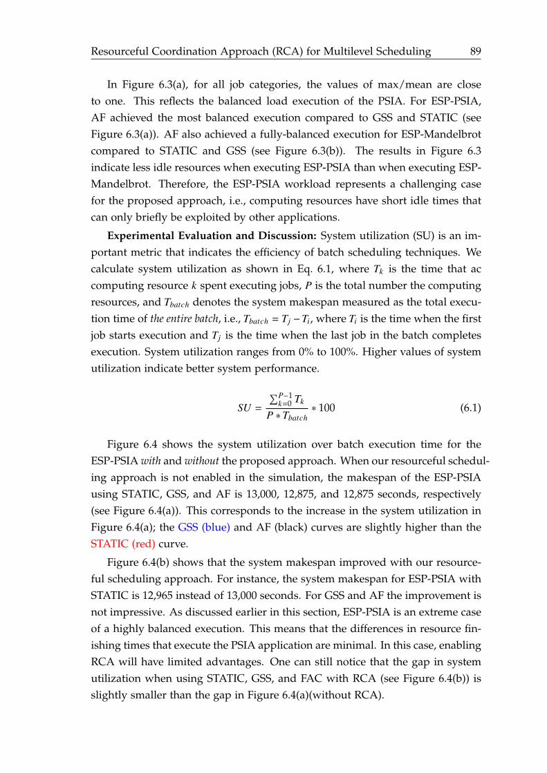
Resourceful Coordination Approach (RCA) for Multilevel Scheduling 89
In Figure 6.3(a), for all job categories, the values of max/mean are closeto one. This reflects the balanced load execution of the PSIA. For ESP-PSIA,AF achieved the most balanced execution compared to GSS and STATIC (seeFigure 6.3(a)). AF also achieved a fully-balanced execution for ESP-Mandelbrotcompared to STATIC and GSS (see Figure 6.3(b)). The results in Figure 6.3indicate less idle resources when executing ESP-PSIA than when executing ESP-Mandelbrot. Therefore, the ESP-PSIA workload represents a challenging casefor the proposed approach, i.e., computing resources have short idle times thatcan only briefly be exploited by other applications.
Experimental Evaluation and Discussion: System utilization (SU) is an im-portant metric that indicates the efficiency of batch scheduling techniques. Wecalculate system utilization as shown in Eq. 6.1, where Tk is the time that accomputing resource k spent executing jobs, P is the total number the computingresources, and Tbatch denotes the system makespan measured as the total execu-tion time of the entire batch, i.e., Tbatch = Tj −Ti, where Ti is the time when the firstjob starts execution and Tj is the time when the last job in the batch completesexecution. System utilization ranges from 0% to 100%. Higher values of systemutilization indicate better system performance.
SU =∑P−1
k=0 Tk
P ∗Tbatch∗ 100 (6.1)
Figure 6.4 shows the system utilization over batch execution time for theESP-PSIA with and without the proposed approach. When our resourceful schedul-ing approach is not enabled in the simulation, the makespan of the ESP-PSIAusing STATIC, GSS, and AF is 13,000, 12,875, and 12,875 seconds, respectively(see Figure 6.4(a)). This corresponds to the increase in the system utilization inFigure 6.4(a); the GSS (blue) and AF (black) curves are slightly higher than theSTATIC (red) curve.
Figure 6.4(b) shows that the system makespan improved with our resource-ful scheduling approach. For instance, the system makespan for ESP-PSIA withSTATIC is 12,965 instead of 13,000 seconds. For GSS and AF the improvement isnot impressive. As discussed earlier in this section, ESP-PSIA is an extreme caseof a highly balanced execution. This means that the differences in resource fin-ishing times that execute the PSIA application are minimal. In this case, enablingRCA will have limited advantages. One can still notice that the gap in systemutilization when using STATIC, GSS, and FAC with RCA (see Figure 6.4(b)) isslightly smaller than the gap in Figure 6.4(a)(without RCA).
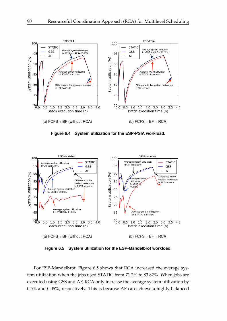
90 Resourceful Coordination Approach (RCA) for Multilevel Scheduling
(a) FCFS + BF (without RCA) (b) FCFS + BF + RCA
Figure 6.4 System utilization for the ESP-PSIA workload.
(a) FCFS + BF (without RCA) (b) FCFS + BF + RCA
Figure 6.5 System utilization for the ESP-Mandelbrot workload.
For ESP-Mandelbrot, Figure 6.5 shows that RCA increased the average sys-tem utilization when the jobs used STATIC from 71.2% to 83.82%. When jobs areexecuted using GSS and AF, RCA only increase the average system utilization by0.5% and 0.05%, respectively. This is because AF can achieve a highly balanced
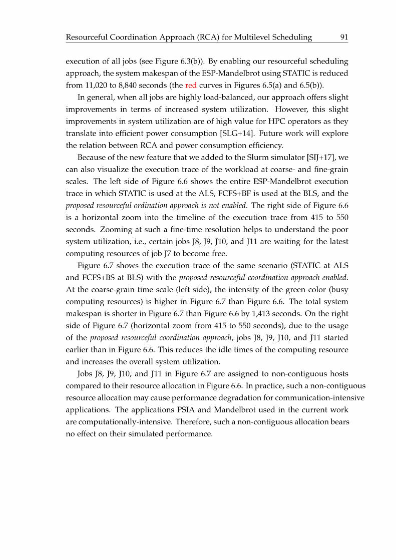
Resourceful Coordination Approach (RCA) for Multilevel Scheduling 91
execution of all jobs (see Figure 6.3(b)). By enabling our resourceful schedulingapproach, the system makespan of the ESP-Mandelbrot using STATIC is reducedfrom 11,020 to 8,840 seconds (the red curves in Figures 6.5(a) and 6.5(b)).
In general, when all jobs are highly load-balanced, our approach offers slightimprovements in terms of increased system utilization. However, this slightimprovements in system utilization are of high value for HPC operators as theytranslate into efficient power consumption [SLG+14]. Future work will explorethe relation between RCA and power consumption efficiency.
Because of the new feature that we added to the Slurm simulator [SIJ+17], wecan also visualize the execution trace of the workload at coarse- and fine-grainscales. The left side of Figure 6.6 shows the entire ESP-Mandelbrot executiontrace in which STATIC is used at the ALS, FCFS+BF is used at the BLS, and theproposed resourceful ordination approach is not enabled. The right side of Figure 6.6is a horizontal zoom into the timeline of the execution trace from 415 to 550seconds. Zooming at such a fine-time resolution helps to understand the poorsystem utilization, i.e., certain jobs J8, J9, J10, and J11 are waiting for the latestcomputing resources of job J7 to become free.
Figure 6.7 shows the execution trace of the same scenario (STATIC at ALSand FCFS+BS at BLS) with the proposed resourceful coordination approach enabled.At the coarse-grain time scale (left side), the intensity of the green color (busycomputing resources) is higher in Figure 6.7 than Figure 6.6. The total systemmakespan is shorter in Figure 6.7 than Figure 6.6 by 1,413 seconds. On the rightside of Figure 6.7 (horizontal zoom from 415 to 550 seconds), due to the usageof the proposed resourceful coordination approach, jobs J8, J9, J10, and J11 startedearlier than in Figure 6.6. This reduces the idle times of the computing resourceand increases the overall system utilization.
Jobs J8, J9, J10, and J11 in Figure 6.7 are assigned to non-contiguous hostscompared to their resource allocation in Figure 6.6. In practice, such a non-contiguousresource allocation may cause performance degradation for communication-intensiveapplications. The applications PSIA and Mandelbrot used in the current workare computationally-intensive. Therefore, such a non-contiguous allocation bearsno effect on their simulated performance.
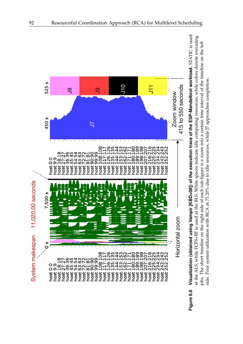
92 Resourceful Coordination Approach (RCA) for Multilevel Scheduling
Hor
izont
al z
oom
Zo
om w
indo
w
415
to 5
50 s
econ
ds
J3
J1J4 J5 J6 J7
Syst
em m
akes
pan
J7J9 J1
0
J11
11,0
20.0
0 se
cond
s
J8
Figu
re6.
6V
isua
lizat
ion
(obt
aine
dus
ing
Vam
pir
[KB
D+0
8])o
fthe
exec
utio
ntr
ace
ofth
eE
SP
-Man
delb
rotw
orkl
oad.
STA
TIC
isus
edat
the
ALS
,whi
leFC
FS+B
Fis
used
atth
eBL
S.W
hite
spac
esin
dica
teid
leco
mpu
ting
reso
urce
s,w
hile
colo
rsde
note
exec
utin
gjo
bs.T
hesh
ort
tim
elin
eon
the
righ
tsi
deof
each
sub-
figur
eis
azo
omin
toa
cert
ain
tim
ein
terv
alof
the
tim
elin
eon
the
left
side
.Poo
rsy
stem
utili
zati
onw
ith
RC
Aat
71.2
0%du
eto
idle
reso
urce
s,w
hile
J7ap
proa
ches
com
plet
ion.
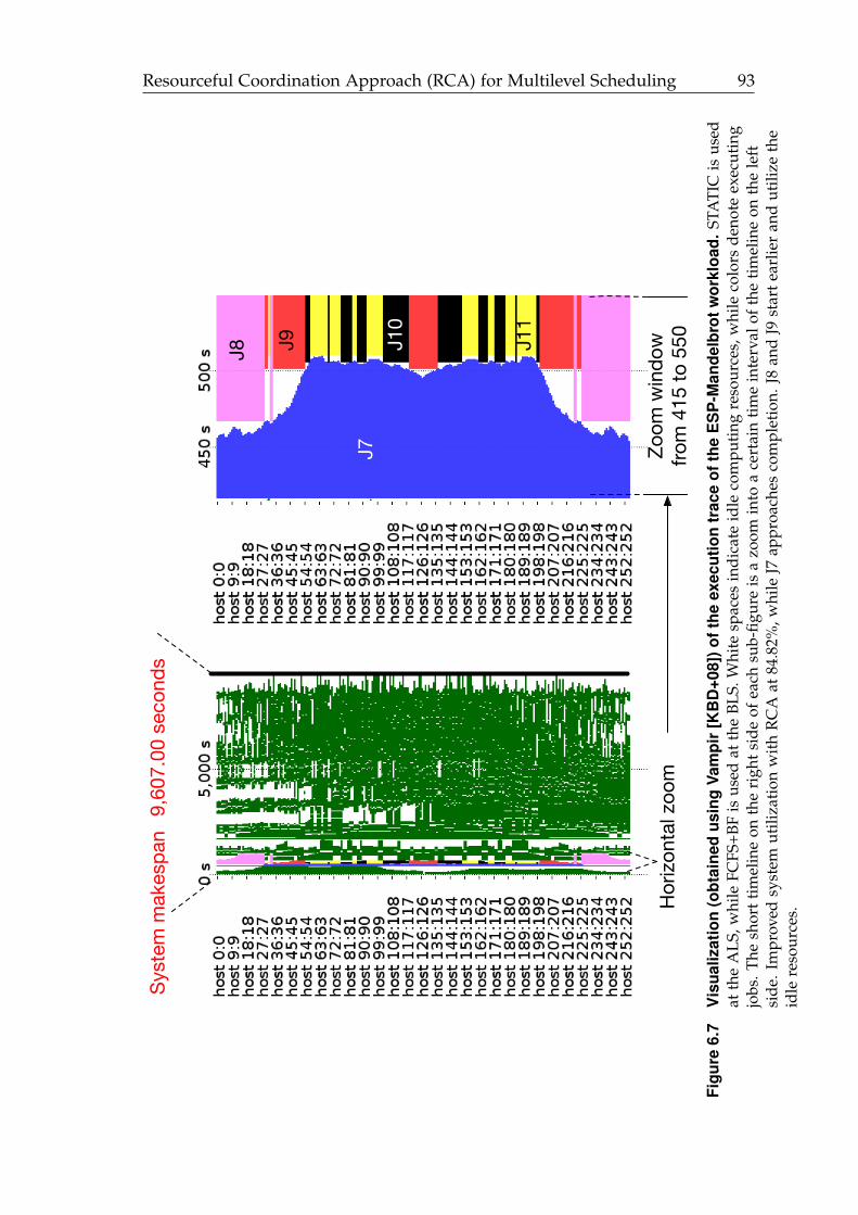
Resourceful Coordination Approach (RCA) for Multilevel Scheduling 93
Horiz
onta
l zoo
m
Zoom
win
dow
fro
m 4
15 to
550
J3
J1
J4 J5 J6
JOB7
J10
9,60
7.00
sec
onds
J7
J8 J9 J10
J11
Syst
em m
akes
pan
Figu
re6.
7V
isua
lizat
ion
(obt
aine
dus
ing
Vam
pir
[KB
D+0
8])o
fthe
exec
utio
ntr
ace
ofth
eE
SP
-Man
delb
rotw
orkl
oad.
STA
TIC
isus
edat
the
ALS
,whi
leFC
FS+B
Fis
used
atth
eBL
S.W
hite
spac
esin
dica
teid
leco
mpu
ting
reso
urce
s,w
hile
colo
rsde
note
exec
utin
gjo
bs.T
hesh
ort
tim
elin
eon
the
righ
tsi
deof
each
sub-
figur
eis
azo
omin
toa
cert
ain
tim
ein
terv
alof
the
tim
elin
eon
the
left
side
.Im
prov
edsy
stem
utili
zati
onw
ith
RC
Aat
84.8
2%,w
hile
J7ap
proa
ches
com
plet
ion.
J8an
dJ9
star
tea
rlie
ran
dut
ilize
the
idle
reso
urce
s.
94 Resourceful Coordination Approach (RCA) for Multilevel Scheduling
6.4 Summary
This chapter showed the resourceful coordination approach (RCA) that allowsapplication schedulers to cooperate by involving the batch scheduler. The pro-posed approach is implemented in a two-level scheduling simulator using realis-tic and well-known simulators (a Slurm-based simulator [SIJ+17] and a SimGrid-basedsimulator [MEC+20]). The effective system performance (ESP) benchmark wasused to assess the proposed approach. ESP jobs were instantiated with the par-allel spin-image generation and the Mandelbrot set.
RCA increased the entire system utilization by 12.6% and decreased the sys-tem makespan by the same percentage when the applications had a severe loadimbalance. System utilization was slightly improved by 0.05% when applicationshad balanced execution. These improvements are of high value for HPC oper-ators as they translate to efficient power consumption [SLG+14]. The presentwork also shows that for long-executing HPC applications, exploiting comput-ing resources’ idle times (in the order of a few seconds) can significantly improvethe entire system utilization. Prior to this work, it was commonly accepted thatshort computing resource idle times filled by Big Data workloads [MGG+17].The current work highlighted the potential of exploring such idle times also forHPC workloads as well.
The proposed extensions to the Slurm-simulator [SIJ+17] enabled the visualanalysis of the workload execution at coarse- and fine-grain temporal resolu-tions using Vampir [KBD+08]. With RCA, the visual analysis showed that idleresources were exploited efficiently and jobs were not assigned to contiguouscomputing resources. Such a non-contiguous resource allocation may cause per-formance degradation of communication-intensive applications, which were notin the scope of the present work but planned as future work.
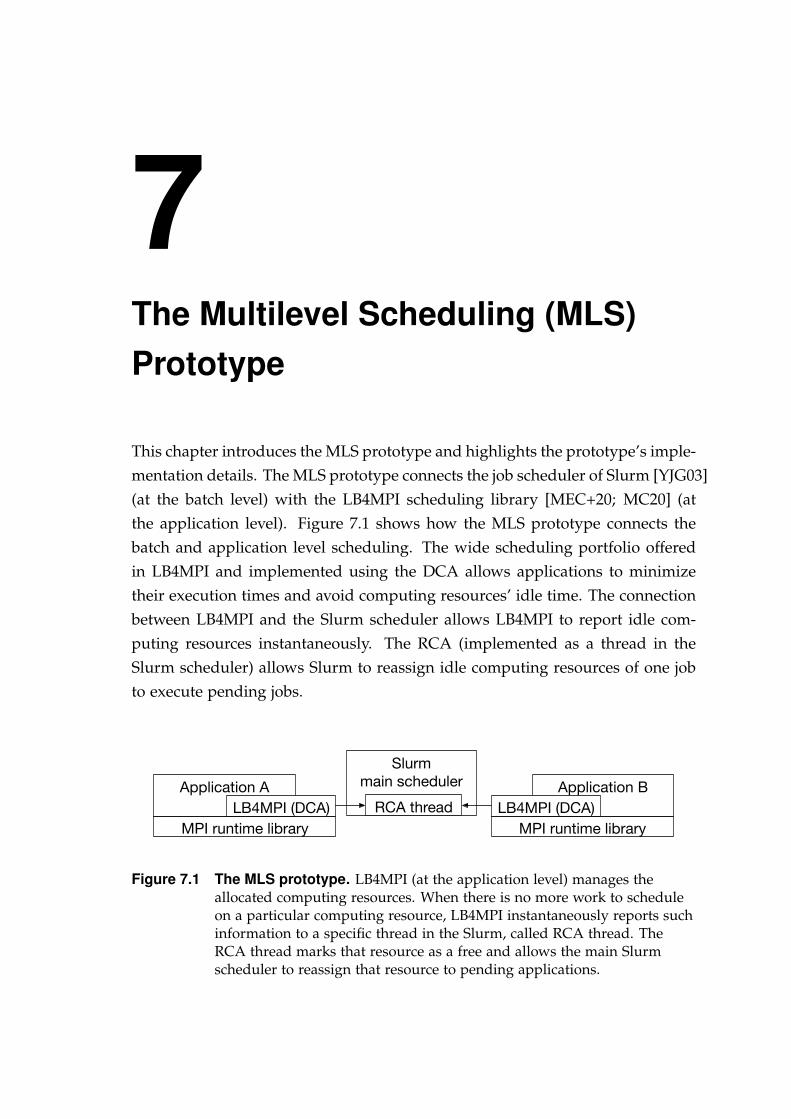
7The Multilevel Scheduling (MLS)Prototype
This chapter introduces the MLS prototype and highlights the prototype’s imple-mentation details. The MLS prototype connects the job scheduler of Slurm [YJG03](at the batch level) with the LB4MPI scheduling library [MEC+20; MC20] (atthe application level). Figure 7.1 shows how the MLS prototype connects thebatch and application level scheduling. The wide scheduling portfolio offeredin LB4MPI and implemented using the DCA allows applications to minimizetheir execution times and avoid computing resources’ idle time. The connectionbetween LB4MPI and the Slurm scheduler allows LB4MPI to report idle com-puting resources instantaneously. The RCA (implemented as a thread in theSlurm scheduler) allows Slurm to reassign idle computing resources of one jobto execute pending jobs.
Slurm main scheduler
MPI runtime library
Application ALB4MPI (DCA) RCA thread
MPI runtime library
Application BLB4MPI (DCA)
Figure 7.1 The MLS prototype. LB4MPI (at the application level) manages theallocated computing resources. When there is no more work to scheduleon a particular computing resource, LB4MPI instantaneously reports suchinformation to a specific thread in the Slurm, called RCA thread. TheRCA thread marks that resource as a free and allows the main Slurmscheduler to reassign that resource to pending applications.
96 The Multilevel Scheduling (MLS) Prototype
7.1 DCA in a Scheduling and Load BalancingLibrary
LB4MPI 1 [MEC+20; MC20] is a recent MPI-based library for loop schedulingand dynamic load balancing. LB4MPI extends the LB tool [CB05] by includingcertain bug fixes and additional DLS techniques. LB4MPI has been used to en-hance the performance of various scientific applications [MC20]. We extend theLB4MPI in two directions: (1) We enable the support of DCA. All the DLS tech-niques originally supported in LB4MPI were implemented with a centralizedchunk calculation approach (CCA), as shown in Figure 7.2. We re-implementthem with DCA, as shown in Figure 7.3. (2) We add six additional DLS tech-niques and implement them with CCA and DCA. These DLS techniques areTAP [Luc92], TFSS [CAB+01], FISS [PD97], VISS [PD97], RND [CIB18], andPLS [SYT07].
LB4MPI has six API functions: DLS_Parameters_Setup, DLS_StartLoop, DLS_-Terminated, DLS_StartChunk, DLS_EndChunk, and DLS_EndLoop. For backwardcompatibility reasons, our extension of LB4MPI maintained the six originalAPIs and their signature. However, we added a new API: Configure_Chunk_-Calculation_Mode that selects between CCA and DCA. We changed each of thesix APIs’ functionality to include a condition that checks the selected approach(CCA or DCA). When the selected approach is CCA, the six APIs work as in theoriginal LB4MPI. For instance, DLS_StartChunk calls either DLS_StartChunk_-
Centralized or DLS_StartChunk_Decentralized based on the selected approach.DLS_StartChunk_Centralized is a function that wraps the original CCA of LB4MPI,while DLS_StartChunk_Decentralized provides the newly added functionalitythat supports DCA.
One can use LB4MPI as in Listing 7.1. One important observation regardingListing 7.1 is that LB4MPI does not perform any data exchange related to theallocated chunks. LB4MPI assumes that each MPI process has access to the dataassociated with the loop iterations it executes. The simplest way to ensure thevalidity of this assumption is to replicate the data of all loop iterations across allMPI processes. Users can also centralize or distribute data of the loop iterationsacross all MPI processes. In this case, however, users need to provide a wayto their applications to exchange the required data associated with the loopiterations.
When a worker calls DLS_EndLoop, this means that LB4MPI will not sched-
1 https://github.com/unibas-dmi-hpc/DLS4LB.git
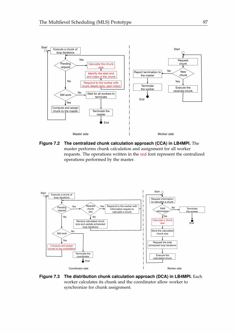
The Multilevel Scheduling (MLS) Prototype 97
Execute a chunk of loop iterations
Pending request
Calculate the chunk size
Identify the start and end index of the chunk
Respond to the worker with chunk details (size, start index)
Compute and assignchunk to the master
Start
Request chunk
New chunk
Start
No
Still work Wait for all workers to terminate
Terminate the master
Yes
Yes
End
Yes
NoReport termination to the master
Terminatethe worker
End
Execute the received chunkNo
Master side Worker side
Figure 7.2 The centralized chunk calculation approach (CCA) in LB4MPI. Themaster performs chunk calculation and assignment for all workerrequests. The operations written in the red font represent the centralizedoperations performed by the master.
Execute a chunk of loop iterations
Pending request
Compute and assignchunk to the coordinator
Start
Request information to calculate a chunk
Valid information
Start
No
Still work
Terminate the coordinator
Yes
Yes
End
Yes
Terminatethe worker
End
Execute the calculated chunk
Coordinator side Worker side
Request chunkinfo
Respond to the worker with information require to
calculate a chunk
Yes
Receive calculated chunk size and update scheduled
loop iterations
No
No
Calculate a chunk size
Send the calculated chunk size
Request the total scheduled loop iterations
No
Figure 7.3 The distribution chunk calculation approach (DCA) in LB4MPI. Eachworker calculates its chunk and the coordinator allow worker tosynchronize for chunk assignment.
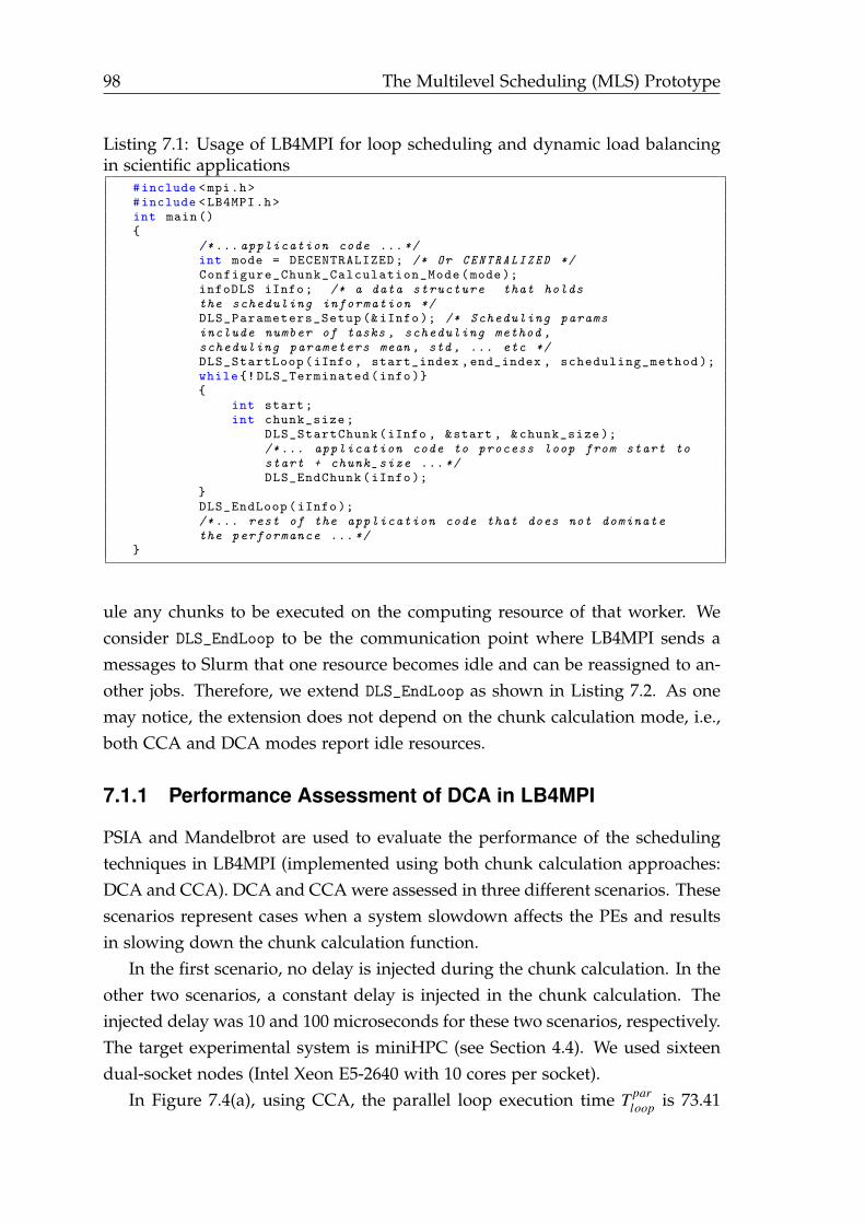
98 The Multilevel Scheduling (MLS) Prototype
Listing 7.1: Usage of LB4MPI for loop scheduling and dynamic load balancingin scientific applications
#include <mpi.h>#include <LB4MPI.h>int main(){
/*... application code ...*/int mode = DECENTRALIZED; /* Or CENTRALIZED */Configure_Chunk_Calculation_Mode(mode);infoDLS iInfo; /* a data structure that holdsthe scheduling information */DLS_Parameters_Setup (&iInfo ); /* Scheduling paramsinclude number of tasks , scheduling method ,scheduling parameters mean , std , ... etc */DLS_StartLoop(iInfo , start_index ,end_index , scheduling_method );while{! DLS_Terminated(info)}{
int start;int chunk_size;
DLS_StartChunk(iInfo , &start , &chunk_size );/*... application code to process loop from start tostart + chunk_size ...*/DLS_EndChunk(iInfo);
}DLS_EndLoop(iInfo );/*... rest of the application code that does not dominatethe performance ...*/
}
ule any chunks to be executed on the computing resource of that worker. Weconsider DLS_EndLoop to be the communication point where LB4MPI sends amessages to Slurm that one resource becomes idle and can be reassigned to an-other jobs. Therefore, we extend DLS_EndLoop as shown in Listing 7.2. As onemay notice, the extension does not depend on the chunk calculation mode, i.e.,both CCA and DCA modes report idle resources.
7.1.1 Performance Assessment of DCA in LB4MPI
PSIA and Mandelbrot are used to evaluate the performance of the schedulingtechniques in LB4MPI (implemented using both chunk calculation approaches:DCA and CCA). DCA and CCA were assessed in three different scenarios. Thesescenarios represent cases when a system slowdown affects the PEs and resultsin slowing down the chunk calculation function.
In the first scenario, no delay is injected during the chunk calculation. In theother two scenarios, a constant delay is injected in the chunk calculation. Theinjected delay was 10 and 100 microseconds for these two scenarios, respectively.The target experimental system is miniHPC (see Section 4.4). We used sixteendual-socket nodes (Intel Xeon E5-2640 with 10 cores per socket).
In Figure 7.4(a), using CCA, the parallel loop execution time T parloop is 73.41
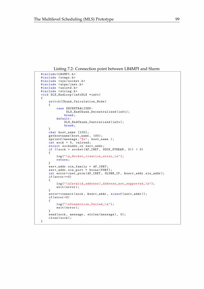
The Multilevel Scheduling (MLS) Prototype 99
Listing 7.2: Connection point between LB4MPI and Slurm#include <LB4MPI.h>#include <utmpx.h>#include <sys/socket.h>#include <arpa/inet.h>#include <unistd.h>#include <string.h>void DLS_EndLoop(infoDLS *info){
switch(Chunk_Calculation_Mode){
case DECENTRALIZED:DLS_EndChunk_Decentralized(info);
break;default:
DLS_EndChunk_Centralized(info);break;
}char host_name [100];gethostname(host_name , 100);sprintf(message ,"%s", host_name );int sock = 0, valread;struct sockaddr_in serv_addr;if ((sock = socket(AF_INET , SOCK_STREAM , 0)) < 0){
log("\n␣Socket␣creation␣error␣\n");return;
}serv_addr.sin_family = AF_INET;serv_addr.sin_port = htons(PORT);int error=inet_pton(AF_INET , SLURM_IP , &serv_addr.sin_addr );if(error <=0){
log("\nInvalid␣address/␣Address␣not␣supported␣\n");exit(error );
}error=connect(sock , &serv_addr , sizeof(serv_addr ));if(error <0){
log("\nConnection␣Failed␣\n");exit(error );
}send(sock , message , strlen(message), 0);close(sock);
}
100 The Multilevel Scheduling (MLS) Prototype
seconds with STATIC, while the best T parloop is 69.37 with FAC2. With FAC2, the
performance of PSIA is enhanced by 5.5%. Other techniques achieve compa-rable performance. For instance, T par
loop is 69.53 seconds with PLS. In contrast,other techniques degrade the performance of PSIA. GSS and RND degrade thePSIA performance by 2.7% and 61.2% compared STATIC. For the DCA, one canmake the same observations regarding the best and the worst techniques. TheCCA and DCA versions of all techniques are comparable to each other, i.e., thedifference in performance ranges from 2% to 3%.
Figures 7.4(b) and 7.4(c) show the performance of both CCA and DCA withdifferent techniques for PSIA when the injected delay is 10 and 100 microsec-onds, respectively. In Figure 7.4(b), one can notice that when the injected delayis 10 microseconds, the performance differences between CCA and DCA withall techniques range from 2% to 3%. Considering the variation in T par
loop of the 20repetitions of each experiment, one observes that both approaches still have acomparable performance.
For the largest injected delay, the DLS techniques implemented with CCAare more sensitive than the DLS techniques implemented with DCA (see Fig-ure 7.4(c)). For Mandelbrot, one can notice the same behavior, i.e., when thereis no injected delay or when the inject delay is 10 microseconds, the perfor-mance differences between CCA and DCA with all techniques are minor (seeFigures 7.5(a) and 7.5(b)). In contrast, Figure 7.5(c) shows that the DCA versionof all the DLS techniques is more capable of maintaining its performance thanthe CCA version.
Another interesting observation is the poor AF performance with CCA (seeFigure 7.5(c)). AF is an adaptive technique, and it accounts for all sources ofload imbalance that affect applications during the execution. However, AF onlyconsiders mupi and σpi. Since we inject the delay in the chunk calculation func-tion, AF cannot account for such a delay, and it works similarly to the case ofno injected delay. Considering the Mandelbrot application’s characteristics, themajority of the AF chunks are equal to 1 loop iterations. This fine chunk sizeleads to an increased number of chunks, i.e., the performance significantly de-creased because the injected delay is proportional to the total number of chunks.For PSIA, the corresponding AF implementation (with CCA) does not have thesame extreme poor performance (see Figure 7.4(c)) because the AF chunk sizesin the case of PSIA are larger than the chunk sizes in the case of Mandelbrot.
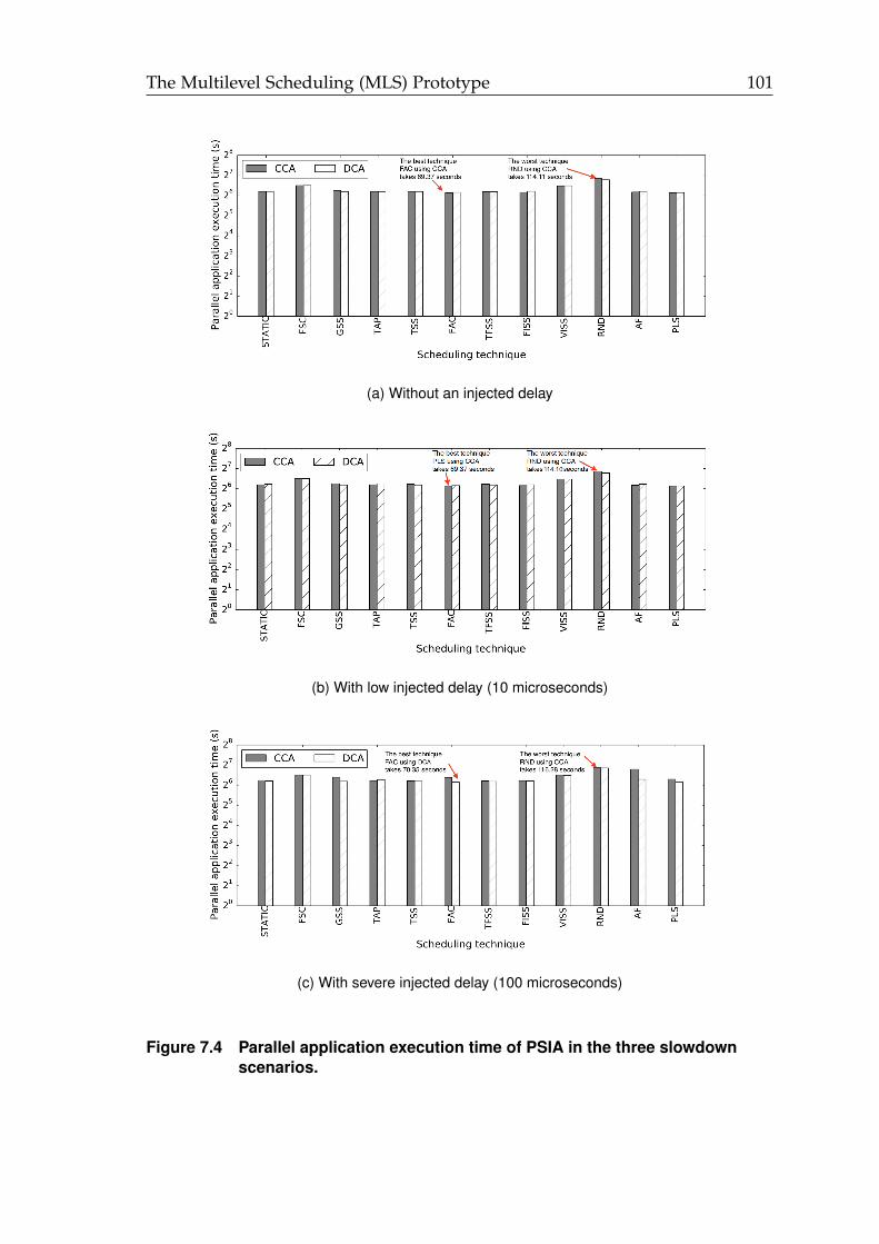
The Multilevel Scheduling (MLS) Prototype 101
(a) Without an injected delay
(b) With low injected delay (10 microseconds)
(c) With severe injected delay (100 microseconds)
Figure 7.4 Parallel application execution time of PSIA in the three slowdownscenarios.
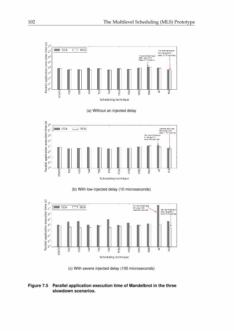
102 The Multilevel Scheduling (MLS) Prototype
(a) Without an injected delay
(b) With low injected delay (10 microseconds)
(c) With severe injected delay (100 microseconds)
Figure 7.5 Parallel application execution time of Mandelbrot in the threeslowdown scenarios.
The Multilevel Scheduling (MLS) Prototype 103
7.2 RCA in a Production Batch Scheduler
Slurm is an open-source software, which is commonly used to manage HPCclusters in government laboratories, universities, and companies worldwide.Since Slurm was introduced in 2003 and until now, its usage constantly spreadsin the HPC community. For instance, in 2013, Slurm was used on 50% of theten most powerful supercomputers [Sch20]. Slurm has a unique design thatrelies on three components that interact to manage jobs’ execution and systemresources. Figure 7.6 shows the main three components of Slurm: slurmctld,slurmd, and slurmdbd.
The slurmd component is a multithreaded daemon (a process that executesin the background). Each computing node executes a single slurmd daemon.Every slurmd daemon notifies about the status of its compute node. The slurmddaemons are responsible for executing jobs on their resources and exchangingjob and node status with the slurmctld daemon (main controller).
The slurmdbd component is another daemon that is responsible for storingthe job accounting information. The job accounting information includes jobarrival time, request resource, start time, execution time, etc. The user can queryjob accounting information with a command utility, called sacct. The slurmdbdeither interfaces with a database server to store the job accounting informationor directly writes job information to an ordinary file as plain text.
The slurmctld component, also known as the main controller, is the centralcomponent of Slurm. It has three responsibilities:
– Polling slurmd daemons to receive their periodic updates to ensures thatnodes their intended configuration
– Gathering nodes into local groups, called partitions. The partitions areused to apply a common configuration to a group of compute nodes.For instance, jobs submitted to a specific partition should finish executionwithin a time limit.
– Scheduling jobs by accepting user jobs, assigning jobs to compute nodes,and adding pending jobs in a priority ordered queue. Jobs can be pendingbecause there are insufficient compute nodes to start.
The slurmctld daemon has a unique multithreaded design that preferably re-quires the slurmctld daemon to execute on a dedicated node, called a headnode. The slurmctld daemon carries out its responsibilities by spinning off sev-eral threads. Certain threads have the lifetime of the slurmctld daemon.
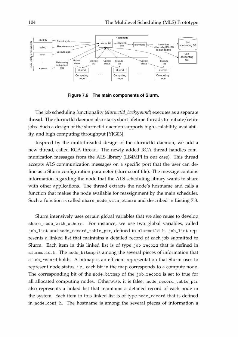
104 The Multilevel Scheduling (MLS) Prototype
Head node
slurmctld slurmdbdStore job info
Computing node
slurmd
Computing node
slurmd
Computing node
slurmd
Updatestatus
Execute job
Execute job
Updatestatus
Updatestatus
Execute job
Job accounting DBInsert data
either in MySQL DBor plain text file
Job accounting
file
salloc
sbatch
srun
squeue
Submit a job
Allocate resource
Execute a job
List running and queued
jobsuser
util
ity c
omm
ands
Figure 7.6 The main components of Slurm.
The job scheduling functionality (slurmctld_background) executes as a separatethread. The slurmctld daemon also starts short lifetime threads to initiate/retirejobs. Such a design of the slurmctld daemon supports high scalability, availabil-ity, and high computing throughput [YJG03].
Inspired by the multithreaded design of the slurmctld daemon, we add anew thread, called RCA thread. The newly added RCA thread handles com-munication messages from the ALS library (LB4MPI in our case). This threadaccepts ALS communication messages on a specific port that the user can de-fine as a Slurm configuration parameter (slurm.conf file). The message containsinformation regarding the node that the ALS scheduling library wants to sharewith other applications. The thread extracts the node’s hostname and calls afunction that makes the node available for reassignment by the main scheduler.Such a function is called share_node_with_others and described in Listing 7.3.
Slurm intensively uses certain global variables that we also reuse to developshare_node_with_others. For instance, we use two global variables, calledjob_list and node_record_table_ptr, defined in slurmctld.h. job_list rep-resents a linked list that maintains a detailed record of each job submitted toSlurm. Each item in this linked list is of type job_record that is defined inslurmctld.h. The node_bitmap is among the several pieces of information thata job_record holds. A bitmap is an efficient representation that Slurm uses torepresent node status, i.e., each bit in the map corresponds to a compute node.The corresponding bit of the node_bitmap of the job_record is set to true forall allocated computing nodes. Otherwise, it is false. node_record_table_ptr
also represents a linked list that maintains a detailed record of each node inthe system. Each item in this linked list is of type node_record that is definedin node_conf.h. The hostname is among the several pieces of information a
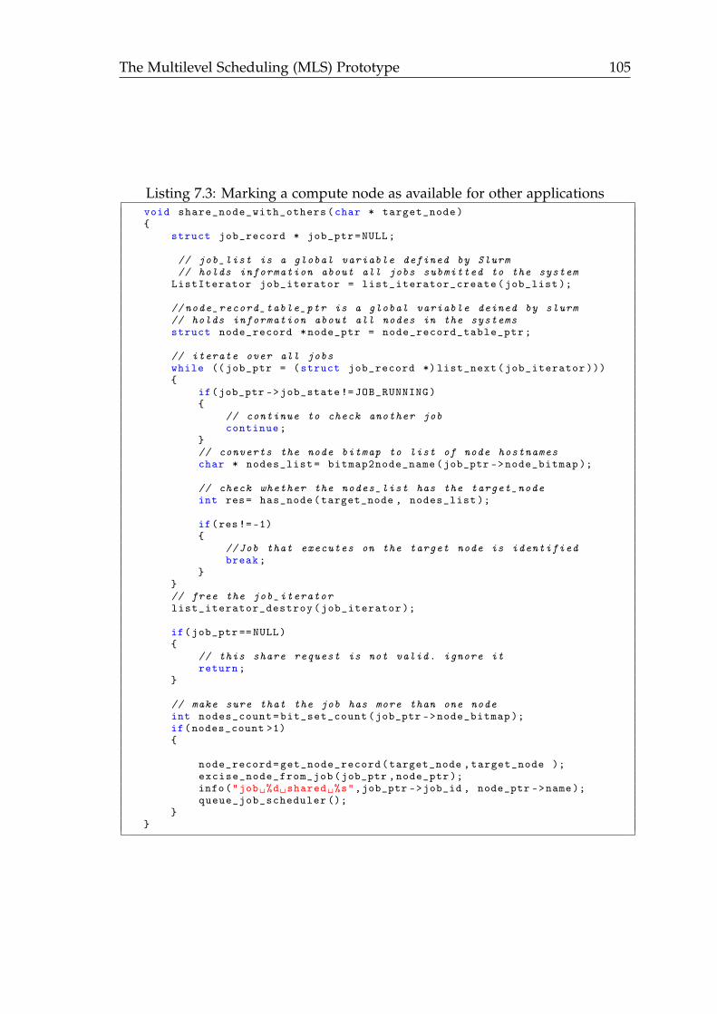
The Multilevel Scheduling (MLS) Prototype 105
Listing 7.3: Marking a compute node as available for other applicationsvoid share_node_with_others(char * target_node){
struct job_record * job_ptr=NULL;
// job_list is a global variable defined by Slurm// holds information about all jobs submitted to the system
ListIterator job_iterator = list_iterator_create(job_list );
// node_record_table_ptr is a global variable deined by slurm// holds information about all nodes in the systemsstruct node_record *node_ptr = node_record_table_ptr;
// iterate over all jobswhile (( job_ptr = (struct job_record *) list_next(job_iterator ))){
if(job_ptr ->job_state != JOB_RUNNING){
// continue to check another jobcontinue;
}// converts the node bitmap to list of node hostnameschar * nodes_list= bitmap2node_name(job_ptr ->node_bitmap );
// check whether the nodes_list has the target_nodeint res= has_node(target_node , nodes_list );
if(res!=-1){
//Job that executes on the target node is identifiedbreak;
}}// free the job_iteratorlist_iterator_destroy(job_iterator );
if(job_ptr ==NULL){
// this share request is not valid. ignore itreturn;
}
// make sure that the job has more than one nodeint nodes_count=bit_set_count(job_ptr ->node_bitmap );if(nodes_count >1){
node_record=get_node_record(target_node ,target_node );excise_node_from_job(job_ptr ,node_ptr );info("job␣%d␣shared␣%s",job_ptr ->job_id , node_ptr ->name);queue_job_scheduler ();
}}
106 The Multilevel Scheduling (MLS) Prototype
node_record holds.
The incoming messages (from the ALS library) contain only the hostname ofthe node to be shared. The message has no information about the job itself(job id, allocated nodes, start time, execution constraints, etc.). The logic inshare_node_with_others has two parts; the first part is to identify the job thatis associated with the incoming message; the second part is to free and reassignthe resource(s) identified in the incoming message.
In the first part, the code iterates overall jobs in the job_list, and uses thenode_bitmap of each job_record in the job_list to check whether the hostnamein the message belongs to the current job allocation. Once this check returnstrue, the current job_record represents the target job. We also identify thetarget node record by checking the hostname of each job_record in the node_-
record_table_ptr.
In the second part, we use certain functions that are defined in the Slurmsource code. The first function is excise_node_from_job. This function takesthe two input parameters (job_record and node_record) that have been identi-fied in the first part. The two parameters are used by excise_node_from_job toremove the given node from the allocation of the given job as follows. It marksthe node’s corresponding bit in the Slurm’s global bitmaps (idle_node_bitmap,avail_node_bitmap). Marking nodes as available and idle does not mean thatthe job binaries have been killed on the node, i.e., the job executes and ownsthe allocation. However, the scheduling library at the application level will notschedule any tasks on the node. Thus, the node can be shared with other appli-cations via the batch level scheduler.
As discussed before, Slurm has a multithreaded design in which the primaryscheduling function runs on a separate thread. The scheduling thread is peri-odically awakened or whenever scheduling events occur, such as job arrival andcompletion. Therefore, share_node_with_others calls a Slurm function, calledqueue_job_scheduler that immediately causes the main scheduling thread towake up.
7.3 Performance Evaluation and Discussion
Evaluating the MLS prototype in a production system is challenging because itmeans interrupting and disturbing the original RMJS of that production system.Furthermore, all Slurm daemons require root privileges to execute appropri-ately. Therefore, 16 compute nodes were segregated from miniHPC [Cio18] and
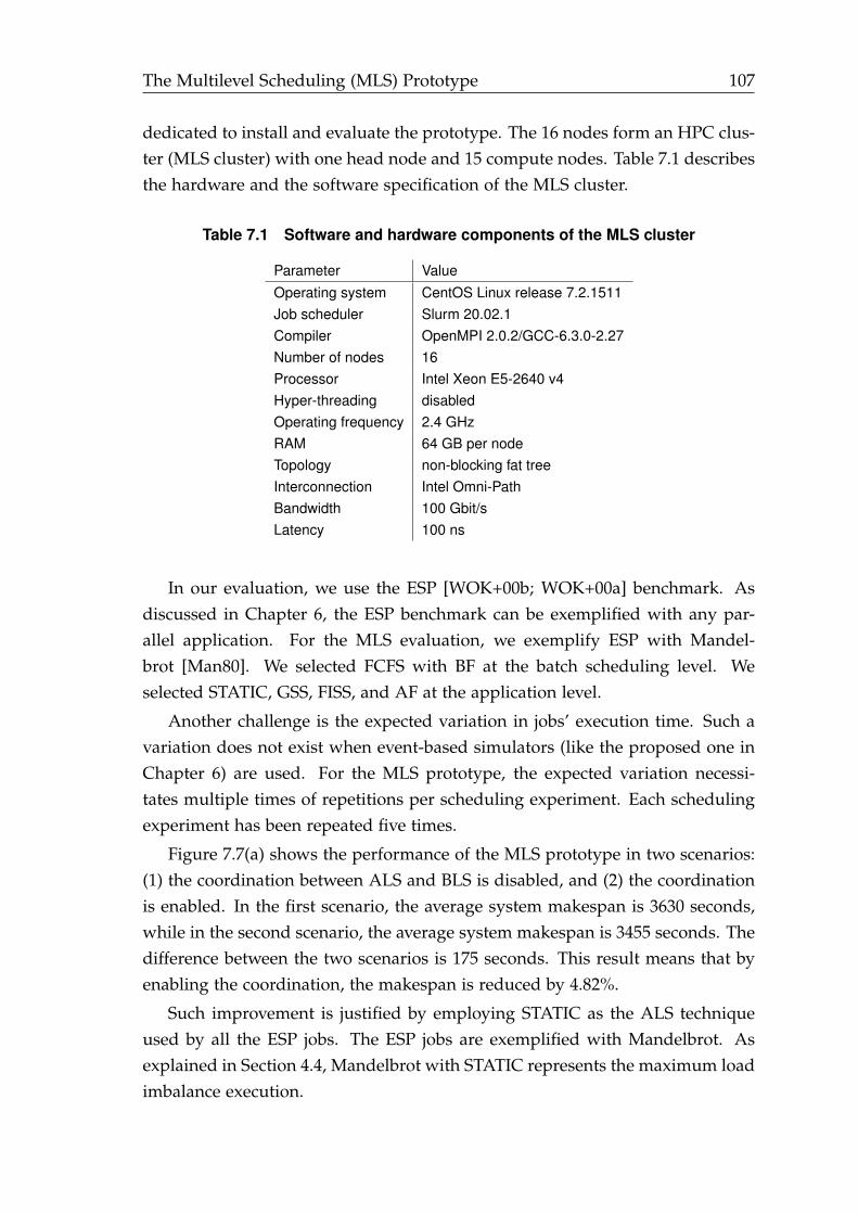
The Multilevel Scheduling (MLS) Prototype 107
dedicated to install and evaluate the prototype. The 16 nodes form an HPC clus-ter (MLS cluster) with one head node and 15 compute nodes. Table 7.1 describesthe hardware and the software specification of the MLS cluster.
Table 7.1 Software and hardware components of the MLS cluster
Parameter ValueOperating system CentOS Linux release 7.2.1511Job scheduler Slurm 20.02.1Compiler OpenMPI 2.0.2/GCC-6.3.0-2.27Number of nodes 16Processor Intel Xeon E5-2640 v4Hyper-threading disabledOperating frequency 2.4 GHzRAM 64 GB per nodeTopology non-blocking fat treeInterconnection Intel Omni-PathBandwidth 100 Gbit/sLatency 100 ns
In our evaluation, we use the ESP [WOK+00b; WOK+00a] benchmark. Asdiscussed in Chapter 6, the ESP benchmark can be exemplified with any par-allel application. For the MLS evaluation, we exemplify ESP with Mandel-brot [Man80]. We selected FCFS with BF at the batch scheduling level. Weselected STATIC, GSS, FISS, and AF at the application level.
Another challenge is the expected variation in jobs’ execution time. Such avariation does not exist when event-based simulators (like the proposed one inChapter 6) are used. For the MLS prototype, the expected variation necessi-tates multiple times of repetitions per scheduling experiment. Each schedulingexperiment has been repeated five times.
Figure 7.7(a) shows the performance of the MLS prototype in two scenarios:(1) the coordination between ALS and BLS is disabled, and (2) the coordinationis enabled. In the first scenario, the average system makespan is 3630 seconds,while in the second scenario, the average system makespan is 3455 seconds. Thedifference between the two scenarios is 175 seconds. This result means that byenabling the coordination, the makespan is reduced by 4.82%.
Such improvement is justified by employing STATIC as the ALS techniqueused by all the ESP jobs. The ESP jobs are exemplified with Mandelbrot. Asexplained in Section 4.4, Mandelbrot with STATIC represents the maximum loadimbalance execution.
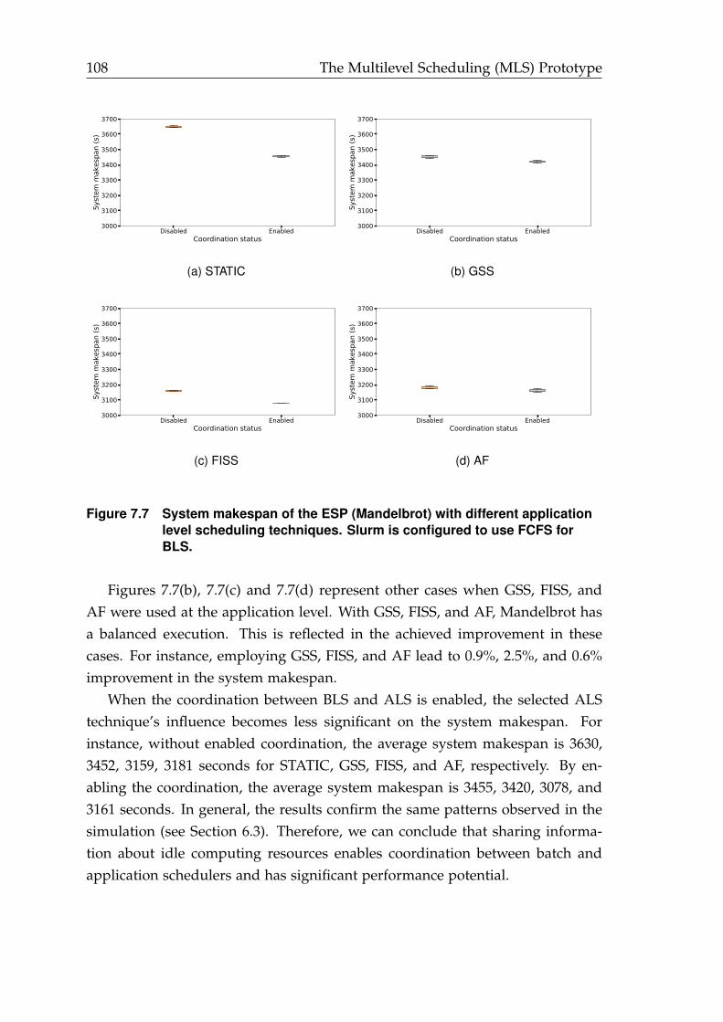
108 The Multilevel Scheduling (MLS) Prototype
Disabled EnabledCoordination status
3000
3100
3200
3300
3400
3500
3600
3700
Syst
em m
akes
pan
(s)
(a) STATIC
Disabled EnabledCoordination status
3000
3100
3200
3300
3400
3500
3600
3700
Syst
em m
akes
pan
(s)
(b) GSS
Disabled EnabledCoordination status
3000
3100
3200
3300
3400
3500
3600
3700
Syst
em m
akes
pan
(s)
(c) FISS
Disabled EnabledCoordination status
3000
3100
3200
3300
3400
3500
3600
3700
Syst
em m
akes
pan
(s)
(d) AF
Figure 7.7 System makespan of the ESP (Mandelbrot) with different applicationlevel scheduling techniques. Slurm is configured to use FCFS forBLS.
Figures 7.7(b), 7.7(c) and 7.7(d) represent other cases when GSS, FISS, andAF were used at the application level. With GSS, FISS, and AF, Mandelbrot hasa balanced execution. This is reflected in the achieved improvement in thesecases. For instance, employing GSS, FISS, and AF lead to 0.9%, 2.5%, and 0.6%improvement in the system makespan.
When the coordination between BLS and ALS is enabled, the selected ALStechnique’s influence becomes less significant on the system makespan. Forinstance, without enabled coordination, the average system makespan is 3630,3452, 3159, 3181 seconds for STATIC, GSS, FISS, and AF, respectively. By en-abling the coordination, the average system makespan is 3455, 3420, 3078, and3161 seconds. In general, the results confirm the same patterns observed in thesimulation (see Section 6.3). Therefore, we can conclude that sharing informa-tion about idle computing resources enables coordination between batch andapplication schedulers and has significant performance potential.
8Conclusions and Future Work
This chapter describes and summarizes the main conclusions that came out ofthe work presented in this doctoral dissertation. This chapter also outlines thefuture extensions of this work.
8.1 Conclusions
Throughout this doctoral dissertation, it has been shown that idle times of com-puting resources towards the end of applications’ execution negatively impactperformance at the batch and application levels. Idle times degrade performanceat the batch level because they decrease system utilization. They also degradeperformance at the application level because they increase applications’ execu-tion time. Therefore, a coordination between schedulers at various levels ofhardware parallelism exploits these idle times.
This conclusion is supported by analyzing simulation results of an exploratorystudy, which has been conducted on workload traces obtained from large-scaleHPC systems in production. The exploratory study includes twelve combina-tions of three BLS and four ALS techniques and is enabled by the two-levelscheduling simulator proposed in Chapter 3.
The two-level scheduling simulator connects two well-known simulators (Grid-Sim and SimGrid), i.e., each simulator is responsible for a certain schedulinglevel. By collecting the simulation events of both simulators and storing theseevents in an OTF2 format, we are able to visualize using Vampir [KBD+08], forthe first time, the system utilization from system to core level. This visualiza-tion allowed us to conclude that coordination absence between BLS and ALStechniques hinders exploiting idle times of computing resources.
110 Conclusions and Future Work
Also, we have learned that the standard workload format (SWF), which wasused to store workload traces for the past two decades, is of limited usefulnessfor simulating BLS and ALS. SWF does not preserve any information abouthow applications schedule their tasks on the allocated resources. To overcomethis limitation, we have proposed the task variation factor that varies the tasks’length within a certain application randomly (see Chapter 3). However, the pro-posed task variation factor does not eliminate the need for storing additionalinformation about how applications schedule their tasks on the allocated re-sources.
Dynamic loop scheduling (DLS) techniques are essential to improve applica-tions’ performance by mitigating all sources of load imbalance. We examinedand assessed the performance of twelve well-known DLS techniques at the ap-plication level. We highlighted a shift in their development. Originally, DLStechniques are devised for shared-memory systems. In the middle of the 1990s,Beowulf clusters and the first MPI standard appeared. Since that time, DLS tech-niques have been implemented on distributed-memory systems by employing amaster-worker execution model that centralizes chunk calculation and chunkassignment at the master side.
We have concluded that the centralization of chunk calculation and chunkassignment contributes to idle times of computing resources, i.e., a worker waitsfor the master to calculate and assign work to all other workers. Thus, the dis-tribution of chunk calculation across all workers is essential for applications’performance. We proposed a distributed chunk calculation approach (DCA)and its hierarchical DCA (HDCA). For both approaches, we have presented theneed for straightforward formulas that do not depend on any information aboutpreviously calculated chunks. We have shown the mathematical transformationrequired to change the formulas of the considered DLS techniques into straight-forward formulas. We recommend to use these straightforward formulas andthe DCA approach for implementing DLS techniques.
Both approaches (DCA and HDCA) are implemented on distributed-memorysystems using the latest features (one-sided communications and MPI sharedmemory) of the latest MPI standard (MPI 3.1). One primary lesson learned isthat the performance of these latest features significantly depends on the MPIruntime library. For instance, the lock polling strategy (employed by Intel MPI)significantly increases scheduling overhead (see Chapter 4). Also, when a largenumber of MPI processes simultaneously access a shared-memory region, theassociated overhead of such an access is higher than the overhead associated
Conclusions and Future Work 111
with simultaneous access of OpenMP threads (see Chapter 5).
In practice, we have observed and learned that none of the considered DLStechniques completely eliminates load imbalance. The considered DLS tech-niques allow computing resources to have nearly equal finishing times, butcomputing resources do not have the exact finishing times, i.e., certain comput-ing resources experience idle times. In this case, we have proposed a resourcefulcoordination approach (RCA) that allows batch systems to exploit computing re-sources once they become free. RCA leverages and combines the advantages ofnode sharing and dynamic resource and job management. It offers an efficientresource sharing (of idle resources only) and avoids shrinkage and expansionoperations on the application side (see Chapter 6).
Employing DCA and RCA in the MLS prototype confirms and promotesour primary conclusion: enabling coordination between batch and applicationschedulers via exchanging scheduling information is crucial to fully exploitcomputing resources of modern HPC systems (see Chapter 7).
8.2 Future Work
Possible extensions can be explored based on the work presented in this the-sis. These possible extensions cover various research directions. In the DLSdirection, recent research efforts [KCY+] expanded specific OpenMP runtime li-braries by adding more DLS techniques. One possible extension is to apply theproposed DCA in such libraries. We also discussed and implemented specificDLS techniques (TFSS, PLS, FISS, and VISS) in the LB4MPI library (see Chap-ters 4 and 7). These techniques have not yet been implemented in any of theOpenMP runtime. Adding these techniques to OpenMP runtime libraries, suchas LLVM, is essential as it widens the scheduling portfolio for selecting the bestperforming scheduling.
Few DLS techniques, such as self-adapting scheduling (SAS) [RCA+06], weredesigned to support scheduling tasks with data dependencies. These techniquesconsider a centralized chunk calculation. Furthermore, they have never beenimplemented in any OpenMP runtime library nor any MPI scheduling library.One immediate extension to our work is to study the potential of applying theproposed DCA to such techniques and implement them in the LLVM OpenMPruntime library and in the LB4MPI library.
Another exciting research direction is how to eliminate the required synchro-nization for the work assignment in the DLS techniques. All DLS techniques

112 Conclusions and Future Work
(except Fractiling [BFH95]) assume a central work queue that necessitates syn-chronization for the work assignment between all workers.
In the direction of batch scheduling, the proposed RCA allows applications toshare their idle computing resources with other applications through the batchsystem. One future extension is to develop batch techniques that use such idleresources to achieve specific performance targets. For instance, a batch techniquethat reuses these idle resources to execute only jobs with short execution timemay increase system throughput.
Furthermore, the current doctoral dissertation focused on idle resource timestowards the end of applications’ execution. One future extension is to study ex-ploiting idle resource times during applications’ execution. Such idle times existin communication-intensive applications, i.e., data transfer between computenodes happens frequently, and in many cases, compute nodes often remain idleuntil the data transfer completes.
With the existing computer technology, parallelism remains the gateway forHPC. Future HPC systems will continue to offer massive parallelism at the core,node, and system levels. Various scheduling techniques are employed to sched-ule computations across all parallelism levels. In this doctoral dissertation, weaddressed the following research problem: the absence of coordination betweenschedulers at different scheduling levels in HPC systems. We have shown how mul-tilevel scheduling efficiently exploits multiple levels of hardware parallelism ofmodern HPC systems.
Bibliography
[ABS+11] Zafril Rizal M. Azmi, Kamalrulnizam Abu Bakar, Mohd ShahirShamsir, Wan Nurulsafawati Manan, and Abdul Hanan Abdul-lah. Scheduling Grid Jobs Using Priority Rule Algorithms andGap Filling Techniques. Journal of Advanced Science and Technology,37:61–76, 2011.
[BSC+12] Mahadevan Balasubramanian, Nitin Sukhija, Florina M. Ciorba,Ioana Banicescu, and Srishti Srivastava. Towards the Scalabilityof Dynamic Loop Scheduling Techniques via Discrete Event Sim-ulation. In Proceedings of the International Parallel and DistributedProcessing Symposium Workshops, 2012, pages 1343–1351.
[BCP+05] Ioana Banicescu, Ricolindo L. Cariño, Jaderick P. Pabico, andMahadevan Balasubramaniam. Design and Implementation of aNovel Dynamic Load Balancing Library for Cluster Computing.Journal of Parallel Computing, 31(7):736–756, 2005.
[BFH95] Ioana Banicescu and Susan Flynn Hummel. Balancing ProcessorLoads and Exploiting Data Locality in N-body Simulations. InProceedings of the International Conference for High Performance Com-puting, Networking, Storage, and Analysis, 1995, pages 43–43.
[BV02] Ioana Banicescu and Vijay Velusamy. Load Balancing Highly Ir-regular Computations With the Adaptive Factoring. In Proceedingsof the International Parallel and Distributed Processing Symposium,2002, 12 pp.
[BVD03] Ioana Banicescu, Vijay Velusamy, and Johnny Devaprasad. Onthe Scalability of Dynamic Scheduling Scientific ApplicationsWith Adaptive Weighted Factoring. Journal of Cluster Computing,6(3):215–226, 2003.
[Ban00] Banicescu, Ioana and Liu, Zhijun. Adaptive Factoring: A Dy-namic Scheduling Method Tuned to the Rate of Weight Changes.In Proceedings of the High performance computing Symposium, 2000,pages 122–129.
114 Bibliography
[BFM+06] Marinho P. Barcellos, Giovani Facchini, Hisham H. Muhammad,Guilherme B. Bedin, and Paulo Luft. Bridging the gap betweensimulation and experimental evaluation in computer networks.In Proceedings of the Annual Simulation Symposium, 2006, 8–pp.
[BCC+04] Kevin Barker, Andrey Chernikov, Nikos Chrisochoides, and Ke-shav Pingali. A Load Balancing Framework for Adaptive andAsynchronous Applications. IEEE Transactions on Parallel and Dis-tributed Systems, 15(2):183–192, 2004.
[BW91] Katherine M. Baumgartner and Benjamin W. Wah. Computerscheduling algorithms: past, present and future. Journal of Infor-mation Sciences, 57:319–345, 1991.
[BG01] Gordon Bell and Jim Gray. High Performance Computing: Crays,Clusters, and Centers. What Next? Communications of the ACM,2001.
[BLR+12] Wes E. Bethel, David Leinweber, Oliver Rübel, and Kesheng Wu.Federal Market Information Technology in the Post–FlashCrashEra: Roles for Supercomputing. The Journal of Trading, 7(2):9–25,2012.
[BLP95] Prashanth B. Bhat, Young Won Lim, and Viktor K. Prasanna. Is-sues in using heterogeneous hpc systems for embedded real timesignal processing applications. In Proceedings of the InternationalWorkshop on Real-Time Computing Systems and Applications, 1995,pages 134–141.
[BDH+15] Mark S. Birrittella, Mark Debbage, Ram Huggahalli, James Kunz,Tom Lovett, Todd Rimmer, Keith D. Underwood, and Robert C.Zak. Intel Omni-Path Architecture: Enabling scalable, high per-formance fabrics. In Proceedings of the Annual Symposium on High-Performance Interconnects, 2015, pages 1–9.
[BCC+97] Susan L. Blackford, Jaeyoung Choi, Andy Cleary, EduardoD’Azevedo, James Demmel, Inderjit Dhillon, Jack Dongarra, SvenHammarling, Greg Henry, Antoine Petitet, et al. ScaLAPACKUsers’ Guide, 1997.
[BBHB+07] Guy E. Blelloch, Lenore Blum, Mor Harchol-Balter, and RobertHarper. Multiscale Scheduling: Integrating Competitive and Co-operative Scheduling in Theory and in Practice. http://lambda-
Bibliography 115
the-ultimate.org/node/2337. [Online; accessed 08 August 2020].2007.
[Boa18] OpenMP Architecture Review Board. OpenMP Application Pro-gramming Interface. https://www.openmp.org/wp- content/uploads/OpenMP-API-Specification-5.0.pdf. [Online; accessed23 August 2020]. 2018.
[BMB+13] Joris Borgdorff, Mariusz Mamonski, Bartosz Bosak, Derek Groen,Mohamed Ben Belgacem, Krzysztof Kurowski, and Alfons GHoekstra. Multiscale Computing With the Multiscale ModelingLibrary and Runtime Environment. Journal of Procedia ComputerScience, 18:1097–1105, 2013.
[BWA16] Anthony Boulmier, John White, and Nabil Abdennadher. Towardsa Cloud Based Decision Support System for Solar Map Genera-tion. In Proceedings of the International Conference on Cloud Comput-ing Technology and Science, 2016, pages 230–236.
[BM02] Rajkumar Buyya and Manzur Murshed. GridSim: A Toolkit forthe Modeling and Simulation of Distributed Resource Manage-ment and Scheduling for Grid Computing. Journal of Concur-rency and Computation: Practice and Experience, 14(13-15):1175–1220,2002.
[Can08] Caniou, Yves and Gay, J. -S. Simbatch: An API for Simulatingand Predicting the Performance of Parallel Resources Managedby Batch Systems. In Proceedings of the European Conference on Par-allel Processing, 2008, pages 223–234.
[CB05] Ricolindo L. Cariño and Ioana Banicescu. A Load BalancingTool for Distributed Parallel Loops. Journal of Cluster Computing,8(4):313–321, 2005.
[CB08] Ricolindo L. Cariño and Ioana Banicescu. Dynamic Load Balanc-ing With Adaptive Factoring Methods in Scientific Applications.Journal of Supercomputing, 44(1):41–63, 2008.
[CBR+04] Ricolindo L. Cariño, Ioana Banicescu, Thomas Rauber, andGudula Rünger. Dynamic loop scheduling with processor groups.In Proceedings of the 17th international conference on parallel and dis-tributed computing systems. 2004, pages 78–84.
116 Bibliography
[CGL+14] Henri Casanova, Arnaud Giersch, Arnaud Legrand, Martin Quin-son, and Frédéric Suter. Versatile, Scalable, and Accurate Simula-tion of Distributed Applications and Patforms. Journal of Paralleland Distributed Computing, 74(10):2899–2917, 2014.
[CBL08] Marc Casas, Rosa Badia, and Jesús Labarta. Automatic Analysisof Speedup of MPI Applications. In Proceedings of the InternationalConference on Supercomputing, 2008, pages 349–358.
[CFK+18] Bastien Chopard, Jean-Luc Falcone, Pierre Kunzli, Lourens Veen,and Alfons Hoekstra. Multiscale Modeling: Recent Progress andOpen Questions. Journal of Multiscale and Multidisciplinary Model-ing, Experiments and Design, 1(1):57–68, 2018.
[CW10] Martin J. Chorley and David W. Walker. Performance Analysisof a Hybrid MPI/OpenMP Application on Multi-core clusters.Journal of Computational Science, 1(3):168–174, 2010.
[CAB+01] Anthony T. Chronopoulos, Razvan Andonie, Manuel Benche, andDaniel Grosu. A Class of Loop Self-scheduling for HeterogeneousClusters. In Proceedings of International Conference on Cluster Com-puting, 2001, pages 282–291.
[CPY+05] Anthony T. Chronopoulos, Satish Penmatsa, Ning Yu, and Du Yu.Scalable Loop Self-scheduling Schemes for Heterogeneous Clus-ters. Journal of Computational Science and Engineering, 1(2-4):110–117, 2005.
[CIB18] Florina M. Ciorba, Christian Iwainsky, and Patrick Buder.OpenMP Loop Scheduling Revisited: Making a Case for MoreSchedules. In Proceedings of the 2018 international workshop onopenmp, 2018, pages 21–36.
[Cio18] Ciorba, Florina M. The miniHPC Cluster. https : / / hpc . dmi .
unibas.ch/HPC/miniHPC.html. [Online; accessed 08 August 2020].2018.
[CGJ83] Edward G. Coffman Jr, Michael R. Garey, and David S. Johnson.Dynamic Bin Packing. SIAM Journal on Computing, 12(2):227–258,1983.
Bibliography 117
[CMHG+16] Isaías Comprés, Ao Mo-Hellenbrand, Michael Gerndt, and Hans-Joachim Bungartz. Infrastructure and API Extensions for ElasticExecution of MPI Applications. In Proceedings of the European MPIUsers’ Group Meeting, 2016, pages 82–97.
[DGGL+18] Marco D’Amico, Marta Garcia-Gasulla, Víctor López, AnaJokanovic, Raül Sirvent, and Julita Corbalan. DROM: Enabling Ef-ficient and Effortless Malleability for Resource Managers. In Pro-ceedings of the International Conference on Parallel Processing Com-panion, 2018, pages 1–10.
[DJC19] Marco D’Amico, Ana Jokanovic, and Julita Corbalan. Holisticslowdown driven scheduling and resource management for mal-leable jobs. In Proceedings of the International Conference on ParallelProcessing, 2019, page 31.
[DHJ07] Luiz DeRose, Bill Homer, and Dean Johnson. Detecting Appli-cation Load Imbalance on High End Massively Parallel Systems.In Proceedings of European Conference on Parallel Processing, 2007,pages 150–159.
[Don03] Jack Dongarra. High Performance Computing Trends and SelfAdapting Numerical Software. In Proceedings of the InternationalSymposium on High Performance Computing, 2003, pages 1–9.
[Don04] Jack Dongarra. The Boole Lecture. Trends in High PerformanceComputing. Computer Journal, 47(4):399–403, 2004.
[Don20] Jack Dongarra. Report on The Fujitsu Fugaku System. https://www.icl.utk.edu/files/publications/2020/icl-utk-1379-
2020.pdf. [Online; accessed 02 September 2020]. 2020.
[DSS+05] Jack Dongarra, Thomas Sterling, Horst Simon, and ErichStrohmaier. High-performance Computing: Clusters, Constella-tions, MPPs, and Future Directions. Computing in science & engi-neering, 7(2):51–59, 2005.
[EC19a] Ahmed Eleliemy and Florina M. Ciorba. Dynamic Loop Schedul-ing Using MPI Passive-Target Remote Memory Access. In Proceed-ings of the Euromicro International Conference on Parallel, Distributedand Network-based Processing, 2019, pages 75–82.
118 Bibliography
[EC19b] Ahmed Eleliemy and Florina M. Ciorba. Hierarchical DynamicLoop Self-Scheduling on Distributed-Memory Systems Using anMPI+MPI Approach. In Proceedings of the International Parallel andDistributed Processing Symposium Workshops, 2019, pages 689–697.
[EC20] Ahmed Eleliemy and Florina M. Ciorba. A Distributed ChunkCalculation Approach for Self-scheduling of Parallel Applicationson Distributed-memory Systems. Journal of Computational Science,2020, revised and resubmitted.
[EC21] Ahmed Eleliemy and Florina M Ciorba. A Resourceful Coordi-nation Approach for Multilevel Scheduling. In Proceedings of theInternational Conference on High Performance Computing & Simula-tion, 2021.
[EFM+16] Ahmed Eleliemy, Mahmoud Fayze, Rashid Mehmood, Iyad.Katib, and Naif Aljohani. Loadbalancing on Parallel Heteroge-neous Architectures: Spin-image Algorithm on CPU and MIC. InProceedings of the 9th EUROSIM Congress on Modelling and Simula-tion, 2016, pages 623–628.
[EMC16] Ahmed Eleliemy, Ali Mohammed, and Florina M. Ciorba. Sim-ulating Batch and Application Level Scheduling Using GridSimand SimGrid. Extended Abstract at the International Confer-ence for High Performance Computing, Networking, Storage, andAnalysis. 2016.
[EMC17a] Ahmed Eleliemy, Ali Mohammed, and Florina M. Ciorba. Effi-cient Generation of Parallel Spin-images Using Dynamic LoopScheduling. In Proceedings of the 8th International Workshop on Mul-ticore and Multithreaded Architectures and Algorithms in conjunctionwith the 19th IEEE International Conference for High PerformanceComputing and Communications, 2017, page 8.
[EMC17b] Ahmed Eleliemy, Ali Mohammed, and Florina M. Ciorba. Explor-ing the Relation between Two Levels of Scheduling Using a NovelSimulation Approach. In Proceedings of the International Symposiumon Parallel and Distributed Computing, 2017, pages 26–33.
[EWG+11] Dominic Eschweiler, Michael Wagner, Markus Geimer, AndreasKnüpfer, Wolfgang E. Nagel, and Felix Wolf. Open Trace Format2: The Next Generation of Scalable Trace Formats and Support
Bibliography 119
Libraries. In Proceedings of the International Conference on ParallelComputing, 2011, pages 481–490.
[FTY+90] Zhixi Fang, Peiyi Tang, Pen-Chung Yew, and Chuan-Qi Zhu.Dynamic Processor Self-scheduling for General Parallel NestedLoops. IEEE Transactions on Computers, 39(7):919–929, 1990.
[Fei05] Dror G. Feitelson. Parallel Workloads Archive.http://www.cs.huji.ac.il/labs/parallel/workload/. [Online;accessed 08 August 2020]. 2005.
[Fei20] Dror G. Feitelson. Standard Workload Format. http://www.cs.huji.ac.il/labs/parallel/workload/swf.html. [Online; ac-cessed 08 August 2020]. 2020.
[FJ97] Dror G. Feitelson and Morris A Jettee. Improved Utilizationand Responsiveness with Gang Scheduling. In Proceedings of theWorkshop on Job Scheduling Strategies for Parallel Processing, 1997,pages 238–261.
[FR95] Dror G. Feitelson and Larry Rudolph. Parallel Job Scheduling: Is-sues and Approaches. In Proceedings of the Workshop on Job Schedul-ing Strategies for Parallel Processing, 1995, pages 1–18.
[FR96] Dror G. Feitelson and Larry Rudolph. Toward Convergence inJob Schedulers for Parallel Supercomputers. In Proceedings of theWorkshop on Job Scheduling Strategies for Parallel Processing, 1996,pages 1–26.
[FRS+97] Dror G. Feitelson, Larry Rudolph, Uwe Schwiegelshohn, KennethC Sevcik, and Parkson Wong. Theory and Practice in Parallel JobSscheduling. In Proceedings of the Workshop on Job Scheduling Strate-gies for Parallel Processing, 1997, pages 1–34.
[FTK14] Dror G. Feitelson, Dan Tsafrir, and David Krakov. Experiencewith using the Parallel Workloads Archive. Journal of parallel anddistributed computing, 74(10):2967–2982, 2014.
[FW98] Dror G. Feitelson and Ahuva Mu’alem Weil. Utilization and Pre-dictability in Scheduling the IBM SP2 With Backfilling. In Proceed-ings of the Merged International Parallel Processing Symposium andSymposium on Parallel and Distributed Processing, 1998, pages 542–546.
120 Bibliography
[FBP15] Edson Flórez, Carlos J. Barrios, and Johnatan E. Pecero. Methodsfor Job Scheduling on Computational Grids: Review and Com-parison. In Proceedings of latin american high performance computingconference, 2015, pages 19–33.
[FHSU+96] Susan Flynn Hummel, Jeanette Schmidt, R. N. Uma, and JoelWein. Load-sharing in Heterogeneous Systems via Weighted Fac-toring. In Proceedings of the 8th annual ACM symposium on Parallelalgorithms and architectures, 1996, pages 318–328.
[FHSF92] Susan Flynn Hummel, Edith Schonberg, and Lawrence E. Flynn.Factoring: A Method for Scheduling Parallel Loops. Journal ofCommunications of the ACM, 35(8):90–101, 1992.
[For20] MPI Forum. Message-Passing Interface. https : / / www . mpi -
forum.org. [Online; accessed 23 August 2020]. 2020.
[GCL09] Marta Garcia, Julita Corbalan, and Jesus Labarta. LeWI: A Run-time Balancing Algorithm for Nested Parallelism. In Proceedings ofthe International Conference on Parallel Processing, 2009, pages 526–533.
[GGR+15] Eric Gaussier, David Glesser, Valentin Reis, and Denis Trys-tram. Improving Backfilling by Using Machine Learning to Pre-dict Running Times. In Proceedings of the International Conferencefor High Performance Computing, Networking, Storage and Analysis,2015, pages 1–10.
[GH12] Yiannis Georgiou and Matthieu Hautreux. Evaluating Scalabilityand Efficiency of the Resource and Job Management System onLarge HPC Clusters. In Proceedings of the Workshop on Job Schedul-ing Strategies for Parallel Processing, 2012, pages 134–156.
[GAB+96] Martyn F. Guest, Edoardo Apra, David E. Bernholdt, Herbert A.Früchtl, Robert J. Harrison, Ricky A. Kendall, RA Kutteh, X. Long,John B. Nicholas, Jeffrey A. Nichols, et al. High-performanceComputing in Chemistry: NW Chem. Future Generation ComputerSystems, 12(4):273–289, 1996.
[HGC14] Jeff R. Hammond, Sayan Ghosh, and Barbara M. Chapman. Im-plementing OpenSHMEM Using MPI-3 One-sided Communica-tion. In Proceedings on the Workshop on OpenSHMEM and RelatedTechnologies, 2014, pages 44–58.

Bibliography 121
[Hen95] Robert L. Henderson. Job Scheduling Under the Portable BatchSystem. In Proceedings of the Workshop on Job Scheduling Strategiesfor Parallel Processing, 1995, pages 279–294.
[HDB+13] Torsten Hoefler, James Dinan, Darius Buntinas, Pavan Balaji,Brian Barrett, Ron Brightwell, William Gropp, Vivek Kale, andRajeev Thakur. MPI + MPI: a new hybrid approach to par-allel programming with MPI plus shared memory. Computing,95(12):1121–1136, 2013.
[HDT+15] Torsten Hoefler, James Dinan, Rajeev Thakur, Brian Barrett, Pa-van Balaji, William Gropp, and Keith Underwood. Remote Mem-ory Access Programming in MPI-3. ACM Transactions on ParallelComputing, 2(2):9, 2015.
[HCB17] Franziska Hoffeins, Florina M. Ciorba, and Ioana Banicescu. Ex-amining the Reproducibility of Using Dynamic Loop Schedul-ing Techniques in Scientific Applications. In International Paralleland Distributed Processing Symposium Workshops, 2017, pages 1579–1587.
[HKK+03] Matthias Hovestadt, Odej Kao, Axel Keller, and Achim Streit.Scheduling in HPC Resource Management Systems: Queuing vs.Planning. In Proceedings of the Workshop on Job Scheduling Strategiesfor Parallel Processing, 2003, pages 1–20.
[How98] Howell, Fred and McNab, Ross. A Discrete Event Simulation Li-brary for Java. In Proceedings of the International Conference on Web-based Modeling and Simulation, 1998, page 6.
[IBM16] IBM LSF. Queue-Level User-based Fairshare. [Online; accessed 13August 2020]. 2016.
[Joh97] Andrew E. Johnson. Spin-Images: A Representation for 3-D Sur-face Matching. PhD thesis. Robotics Institute, Carnegie MellonUniversity, 1997.
[JTS09] Raka Jovanovic, Milan Tuba, and Dana Simian. A New Visualiza-tion Algorithm for the Mandelbrot Set. In Proceedings of the 10thWSEAS International Conference on Mathematics and Computers inBiology and Chemistry, 2009, pages 162–166.
122 Bibliography
[KR01] Axel Keller and Alexander Reinefeld. Anatomy of A ResourceManagement System for HPC Clusters. Annual review of scalablecomputing, 3(1):1–31, 2001.
[KT11] Volodymyr Kindratenko and Pedro Trancoso. Trends in High-performance Computing. Computing in science & engineering,13(3):92–95, 2011.
[Kis02] Laszlo B Kish. End of Moore’s Law: Thermal (Noise) Death of In-tegration in Micro and Nano Electronics. Physics Letters A, 305(3-4):144–149, 2002.
[KMR07] Dalibor Klusácek, Ludek Matyska, and Hana Rudová. Alea–GridScheduling Simulation Environment. In Proceedings of the Inter-national Conference on Parallel Processing and Applied Mathematics,2007, pages 1029–1038.
[KR10] Dalibor Klusácek and Hana Rudová. Alea 2: Job Scheduling Sim-ulator. In Proceedings of the International Conference on SimulationTools and Techniques, 2010, page 61.
[KR11] Dalibor Klusácek and Hana Rudová. Efficient Grid SchedulingThrough the Incremental Schedule-based Approach. Journal Com-putational Intelligence, 27(1):4–22, 2011.
[KSS19] Dalibor Klusácek, Mehmet Soysal, and Frédéric Suter. Alea -Complex Job Scheduling Simulator. In Proceedings of the Inter-national Conference on Parallel Processing and Applied Mathematics,2019, pages 217–229.
[KBD+08] Andreas Knüpfer, Holger Brunst, Jens Doleschal, Matthias Ju-renz, Matthias Lieber, Holger Mickler, Matthias S Müller, andWolfgang E. Nagel. The Vampir Performance Analysis Tool-set.In Proceedings of the International Workshop on Parallel Tools for HighPerformance Computing, 2008, pages 139–155.
[KCY+] Jonas H. Müller Korndörfer, Florina M. Ciorba, Akan Yilmaz,Christian Iwainsky, Johannes Doerfert, Hal Finkel, Vivek Kale,and Michael Klemm. A Runtime Approach for Dynamic LoadBalancing of OpenMP Parallel Loops in LLVM. Poster at Interna-tional Conference on High Performance Computing, Networking,Storage and Analysis.
Bibliography 123
[KW85] Clyde P. Kruskal and Alan Weiss. Allocating Independent Sub-tasks on Parallel Processors. IEEE Transactions on Software Engi-neering, SE-11(10):1001–1016, 1985.
[LMM+19] Ignacio Laguna, Ryan Marshall, Kathryn Mohror, Martin Rue-fenacht, Anthony Skjellum, and Nawrin Sultana. A Large-scaleStudy of MPI Usage in Open-source HPC Applications. In Pro-ceedings of the International Conference for High Performance Comput-ing, Networking, Storage and Analysis, 2019, page 31.
[LTS+93] H. Li, S. Tandri, M. Stumm, and K. C. Sevcik. Locality and loopscheduling on numa multiprocessors. In Proceedings of the interna-tional conference on parallel processing, 1993, pages 140–147.
[LF03] Uri Lublin and Dror G. Feitelson. The workload on parallel su-percomputers: modeling the characteristics of rigid jobs. Journalof Parallel and Distributed Computing, 63(11):18, 2003.
[Luc92] Steven Lucco. A Dynamic Scheduling Method for Irregular Paral-lel Programs. In Proceedings of the ACM Conference on ProgrammingLanguage Design and Implementation, 1992, pages 200–211.
[Luc11] Alejandro Lucero. Simulation of Batch Scheduling Using RealProduction-ready Software Tools. In Proceedings of the 5th IBER-GRID, 2011.
[Man80] Benoit B. Mandelbrot. Fractal Aspects of the Iteration of z →Λz (1-z) for Complex Λ and z. Journal of Annals of the New YorkAcademy of Sciences, 357(1):249–259, 1980.
[MGG+17] Michael Mercier, David Glesser, Yiannis Georgiou, and OlivierRichard. Big Data and HPC collocation: Using HPC Idle Re-sources for Big Data Analytics. In Proceedings of International Con-ference on Big Data, 2017, pages 347–352.
[MC20] Ali Mohammed and Florina M. Ciorba. SimAS: A Simulation-assisted Approach for the Scheduling Algorithm Selection UnderPerturbations. Concurrency and Computation: Practice and Experi-ence, 32(15):e5648, 2020.
[MEC18] Ali Mohammed, Ahmed Eleliemy, and Florina M. Ciorba. Perfor-mance Reproduction and Prediction of Selected Dynamic LoopScheduling Experiments. In Proceedings of the international confer-
124 Bibliography
ence on high performance computing & simulation, 2018, pages 398–405.
[MEC+18] Ali Mohammed, Ahmed Eleliemy, Florina M. Ciorba, FranziskaKasielke, and Ioana Banicescu. Experimental verification andAnalysis of Dynamic Loop Scheduling in Scientific Applications.In Proceedings of the international symposium on parallel and dis-tributed computing, 2018, pages 141–148.
[MEC+20] Ali Mohammed, Ahmed Eleliemy, Florina M. Ciorba, FranziskaKasielke, and Ioana Banicescu. An Approach for RealisticallySimulating the Performance of Scientific Applications on highPerformance Computing Systems. Journal of Future GenerationComputer Systems, 111:617–633, 2020.
[Moo+65] Gordon E. Moore et al. Cramming More Components onto Inte-grated Circuits. 1965.
[Nag93] Wolfgang E. Nagel. A Distributed Scheduler System for Multi-processor Computers with Shared memory: Investigations intothe Scheduling of Parallel Programs. PhD thesis. RWTH Aachen,1993, pages 1, 174.
[Ope20] OpenMP Architecture Review Board. OpenMP Application Pro-gramming Interface. https://www.openmp.org/wp- content/uploads/OpenMP-API-Specification-5.0.pdf. [Online; accessed10 September 2020]. 2020.
[PGW+17] Arnab K. Paul, Arpit Goyal, Feiyi Wang, Sarp Oral, Ali R. Butt,Michael J. Brim, and Sangeetha B. Srinivasa. I/o Load Balancingfor Big Data HPC Applications. In Proceedings of the internationalconference on big data (big data), 2017, pages 233–242.
[PPC86] Tang Peiyi and Yew Pen-Chung. Processor Self-scheduling forMultiple-nested Parallel Loops. In Proceedings of the InternationalConference on Parallel Processing, 1986, pages 528–535.
[Pfi01] Gregory F. Pfister. An introduction to the Infiniband architecture.High Performance Mass Storage and Parallel I/O, 42:617–632, 2001.
[PD97] Teebu Philip and Chita R Das. Evaluation of Loop Scheduling Al-gorithms on Distributed Memory Systems. In Proceedings of theInternational Conference on Parallel and Distributed Computing Sys-tems, 1997, pages 76–94.
Bibliography 125
[PK87] Constantine D. Polychronopoulos and David J. Kuck. GuidedSelf-Scheduling: A Practical Scheduling Scheme for Parallel Su-percomputers. IEEE Transactions on Computers, 100(12):1425–1439,1987.
[Pra16] Suraj Prabhakaran. Dynamic Resource Management and JobScheduling for High Performance Computing. PhD thesis. Tech-nische Universität Darmstadt, 2016.
[PIR+14] Suraj Prabhakaran, Mohsin Iqbal, Sebastian Rinke, ChristianWindisch, and Felix Wolf. A Batch System With Fair Schedulingfor Evolving Applications. In Proceedings of the International Con-ference on Parallel Processing, 2014, pages 351–360.
[PNR+15] Suraj Prabhakaran, Marcel Neumann, Sebastian Rinke, Felix Wolf,Abhishek Gupta, and Laxmikant V Kale. A Batch System WithEfficient Adaptive Scheduling for Malleable and Evolving Appli-cations. In Proceedings of the International Parallel and DistributedProcessing Symposium, 2015, pages 429–438.
[RBA+18] Albert Reuther, Chansup Byun, William Arcand, David Bestor,Bill Bergeron, Matthew Hubbell, Michael Jones, Peter Michaleas,Andrew Prout, Antonio Rosa, et al. Scalable System Schedulingfor HPC and Big Data. Journal of Parallel and Distributed Computing,111:76–92, 2018.
[RCA+06] I. Riakotakis, F. M. Ciorba, T. Andronikos, and G. Papakonstanti-nou. Self-adapting Scheduling for Tasks with Dependencies inStochastic Environments. In Proceedings of the International Confer-ence on Cluster Computing, 2006, pages 1–8.
[Rod17] Gonzalo P. Rodrigo. HPC Scheduling in a Brave New World. PhDthesis. Umeå Universitet, 2017.
[ST07] K. Y. Sanbonmatsu and C. S. Tung. High Performance Computingin Biology: Multimillion Atom Simulations of Nanoscale Systems.Journal of Structural Biology, 157(3):470–480, 2007.
[SV09] H. A. Sanjay and Sathish S Vadhiyar. A Strategy for SchedulingTightly Coupled Parallel Applications on Clusters. Concurrencyand Computation: Practice and Experience, 21(18):2491–2517, 2009.

126 Bibliography
[SLG+14] Osman Sarood, Akhil Langer, Abhishek Gupta, and LaxmikantKale. Maximizing Throughput of Overprovisioned HPC DataCenters Under a Strict Power Budget. In Proceedings of the Interna-tional Conference for High Performance Computing, Networking, Stor-age and Analysis, 2014, pages 807–818.
[Sch97] Robert R. Schaller. Moore’s Law: Past, Present and Future. IEEESpectrum, 34(6):52–59, 1997.
[Sch20] SchedMD. SchedMD: Slurm Development and Support. https://slurm.schedmd.com/pdfs/schedmd_slurm_data.pdf. [Online;accessed 26 August 2020]. 2020.
[SWZ+16] Hongzhang Shan, Samuel Williams, Yili Zheng, Weiqun Zhang,Bei Wang, Stephane Ethier, and Zhengji Zhao. Experiences of Ap-plying One-sided Communication to Nearest-neighbor Commu-nication. In Proceedings of the Workshop on PGAS Applications, 2016,pages 17–24.
[SYT07] Wen-Chung Shih, Chao-Tung Yang, and Shian-Shyong Tseng. APerformance-based Parallel Loop Scheduling on Grid Environ-ments. Journal of Supercomputing, 41(3):247–267, 2007.
[SDI+18] Nikolay A. Simakov, Robert L. DeLeon, Martins D. Innus,Matthew D. Jones, Joseph P. White, Steven M. Gallo, Abani K. Pa-tra, and Thomas R. Furlani. Slurm Simulator: Improving SlurmScheduler Performance on Large HPC Systems by Utilization ofmultiple Controllers and Node Sharing. In, Proceedings of the Prac-tice and Experience on Advanced Research Computing, pages 1–8,2018.
[SIJ+17] Nikolay A. Simakov, Martins D. Innus, Matthew D. Jones, RobertL. DeLeon, Joseph P. White, Steven M. Gallo, Abani K. Patra,and Thomas R. Furlani. A Slurm Simulator: Implementation andParametric Analysis. In Proceedings of the International Workshop onPerformance Modeling, Benchmarking and Simulation of High Perfor-mance Computer Systems, 2017, pages 197–217.
[SB01] Lorna Smith and Mark Bull. Development of mixed modeMPI/OpenMP applications. Scientific Programming, 9(2-3):83–98,2001.
Bibliography 127
[SBC+11] Srishti Srivastava, Ioana Banicescu, Florina M. Ciorba, and Wolf-gang E. Nagel. Enhancing the Functionality of a GridSim-basedScheduler for Effective Use with Large-Scale Scientific Applica-tions. In Proceedings of the International Symposium on Parallel andDistributed Computing, 2011, pages 86–93.
[STL+15] Luka Stanisic, Samuel Thibault, Arnaud Legrand, Brice Videau,and Jean-François Méhaut. Faithful Performance Prediction of aDynamic Task-based Runtime system for Heterogeneous Multi-core Architectures. Concurrency and Computation: Practice and Ex-perience, 27(16):4075–4090, 2015.
[SVP+10] Tony Stöcker, Kaveh Vahedipour, Daniel Pflugfelder, and N JonShah. High-performance Computing MRI Simulations. Magneticresonance in medicine, 64(1):186–193, 2010.
[SBS+13] Nitin Sukhija, Ioana Banicescu, Srishti Srivastava, and Florina M.Ciorba. Evaluating the Flexibility of Dynamic Loop Schedulingon Heterogeneous Systems in the Presence of Fluctuating LoadUsing SimGrid. In Proceedings of the International Parallel and Dis-tributed Processing Symposium Workshops, 2013, pages 1429–1438.
[TES+19] A. Totounferoush, N. Ebrahimi Pour, J. Schröder, S. Roller,and M. Mehl. A New Load Balancing Approach for CoupledMulti-Physics Simulations. In Proceedings of the international par-allel and distributed processing symposium workshops (ipdpsw), 2019,pages 676–682.
[TN93] Ten H. Tzen and Lionel M. Ni. Trapezoid Self-Scheduling: A Prac-tical Scheduling Scheme for Parallel Compilers. IEEE Transactionson Parallel and Distributed Systems, 4(1):87–98, 1993.
[Ull75] J. D. Ullman. NP-complete Scheduling Problems. Journal of Com-puter and System Sciences, 10(3):384–393, 1975.
[VM02] Jeffrey S. Vetter and Frank Mueller. Communication Characteris-tics of Large-scale Scientific Applications for Contemporary Clus-ter Architectures. In Proceedings of the International Parallel and Dis-tributed Processing Symposium, 2002, 10–pp.
[WLD+10] K. Wang, G. Lavoué, F. Denis, A. Baskurt, and X. He. A Bench-mark for 3D Mesh Watermarking. In Proceedings of the 9th IEEEInternational Conference on Shape Modeling and Applications, 2010,pages 231–235.
128 Bibliography
[WOK+00a] Adrian T. Wong, Leonid Oliker, William Kramer, Teresa L. Kaltz,and David H. Bailey. ESP: A System Utilization Benchmark. InProceedings of the International Conference on Supercomputing, 2000,pages 15–19.
[WOK+00b] Adrian T. Wong, Leonid Oliker, William Kramer, Teresa L. Kaltz,and David H. Bailey. System Utilization Benchmark on the CrayT3E and IBM SP. In Proceedings of the Workshop on Job SchedulingStrategies for Parallel Processing, 2000, pages 56–67.
[WYL+12] Chao-Chin Wu, Chao-Tung Yang, Kuan-Chou Lai, and Po-HsunChiu. Designing Parallel Loop Self-scheduling Schemes Using theHybrid MPI and OpenMP Programming Model for Multi-coreGrid Systems. Journal of Supercomputing, 59(1):42–60, 2012.
[Xha10] Xhafa, Fatos and Abraham, Ajith. Computational Models andHeuristic Methods for Grid Scheduling Problems. Future Gener-ation Computer Systems, 26(4):608–621, 2010.
[YJG03] Andy B. Yoo, Morris A. Jette, and Mark Grondona. Slurm: Sim-ple Linux Utility for Resource Management. In Proceedings of theWorkshop on Job Scheduling Strategies for Parallel Processing, 2003,pages 44–60.
[ZBG16] Xin Zhao, Pavan Balaji, and William Gropp. Scalability Chal-lenges in Current MPI One-Sided Implementations. In Proceedingsof International Symposium on Parallel and Distributed Computing,2016, pages 38–47.
[ZG16] Huan Zhou and José Gracia. Asynchronous Progress Design for aMPI-based PGAS One-sided Communication System. In Proceed-ings of the International Conference on Parallel and Distributed Sys-tems, 2016, pages 999–1006.
Index
AF, 21Alea, 32ALS, 5, 15AWF, 21AWF-B, 21AWF-C, 21AWF-D, 21AWF-E, 21
BF, 25BLS, 5, 24
c.o.v., 22CCA, 96CCS, 25
DCA, 10DLS, 5, 15, 17DSS, 52
EASY BF, 26EDF, 25ESG, 25ESP, 86ESP-Mandelbrot, 87ESP-PSIA, 87
FAC, 17, 19FAC2, 19FCFS, 25FISS, 18, 20FLOP/s, 1FSC, 17, 18Fugaku, 2
GridSim, 32GSS, 17, 18
HDCA, 10HDSS, 52HPC, 1
job, 24
LB tool, 54LSF, 26Lublin, 36
MLS, 4, 81, 95MPI, 32MSG, 31
PBS, 26percent load imbalance, 22Performance, 1PEs, 8PLS, 18, 20PWA, 36, 43, 44
RCA, 10, 81RJMSs, 24RMA, 58RND, 18, 20
S4U, 32Scheduling, 3, 15SD, 31SimGrid, 31SJF, 25SLS, 17Slurm, 26slurmctld, 103slurmd, 103slurmdbd, 103SMPI, 31

130 Index
SS, 17, 18STATIC, 17SU, 27SWF, 32SWR, 20
TAP, 17, 18TFSS, 17, 19TSS, 17, 18
VISS, 18, 20
WF, 17, 19WF2, 19