non-linear strogatz 4

8/3/2019 Non-Linear Strogatz 4

http://slidepdf.com/reader/full/non-linear-strogatz-4 1/4

Non-Linear Dynamics Homework Solutions

Week 4: Strogatz Portion

February 3, 2009

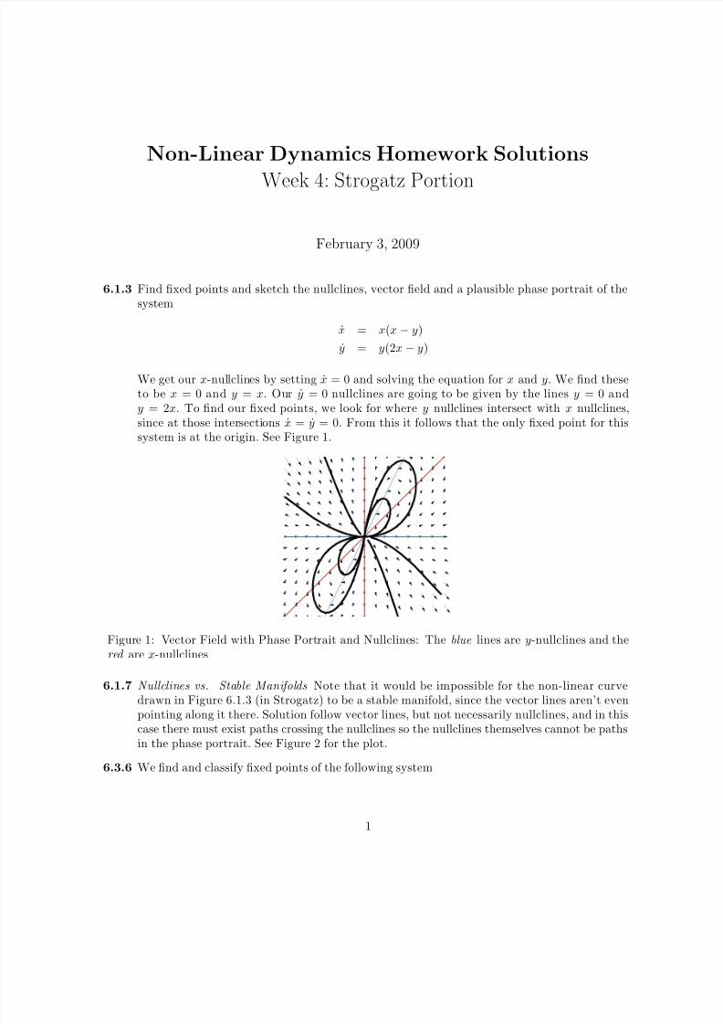
6.1.3 Find fixed points and sketch the nullclines, vector field and a plausible phase portrait of thesystem

x = x(x − y)

y = y(2x − y)

We get our x-nullclines by setting x = 0 and solving the equation for x and y. We find theseto be x = 0 and y = x. Our y = 0 nullclines are going to be given by the lines y = 0 andy = 2x. To find our fixed points, we look for where y nullclines intersect with x nullclines,since at those intersections x = y = 0. From this it follows that the only fixed point for thissystem is at the origin. See Figure 1.

Figure 1: Vector Field with Phase Portrait and Nullclines: The blue lines are y-nullclines and thered are x-nullclines

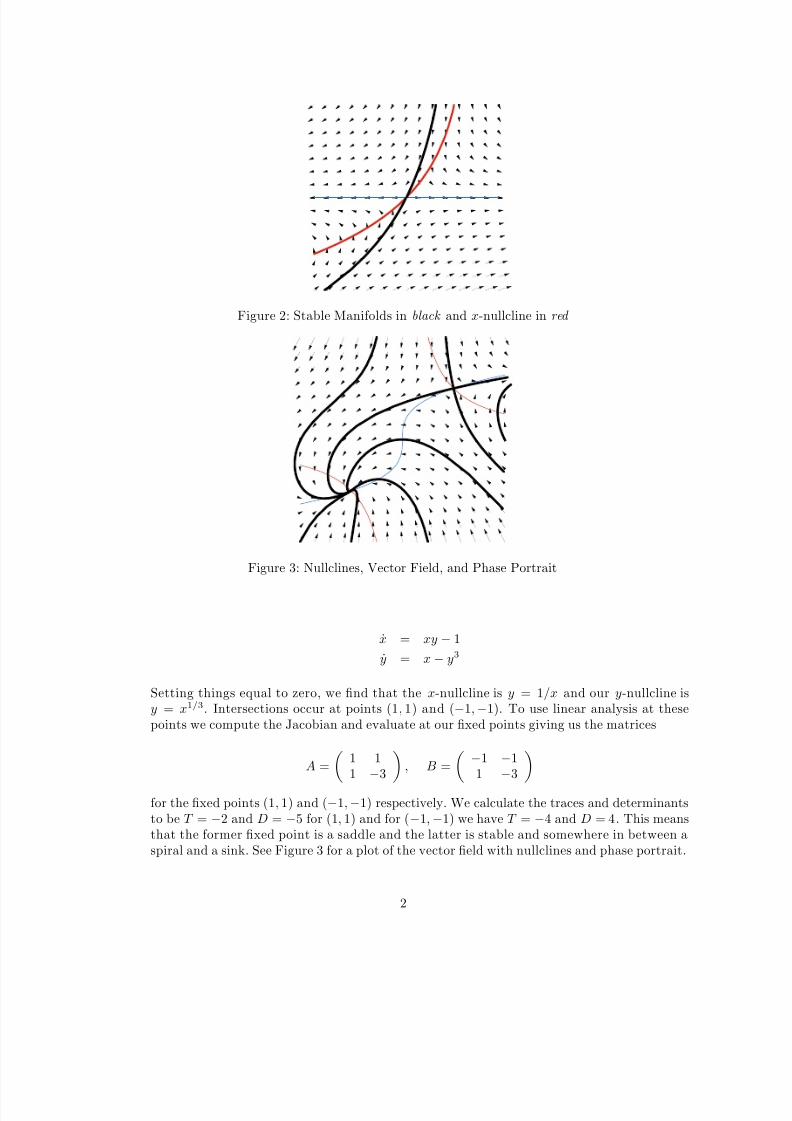
6.1.7 Nullclines vs. Stable Manifolds Note that it would be impossible for the non-linear curvedrawn in Figure 6.1.3 (in Strogatz) to be a stable manifold, since the vector lines aren’t even

pointing along it there. Solution follow vector lines, but not necessarily nullclines, and in thiscase there must exist paths crossing the nullclines so the nullclines themselves cannot be pathsin the phase portrait. See Figure 2 for the plot.

6.3.6 We find and classify fixed points of the following system

1



Figure 2: Stable Manifolds in black and x-nullcline in red

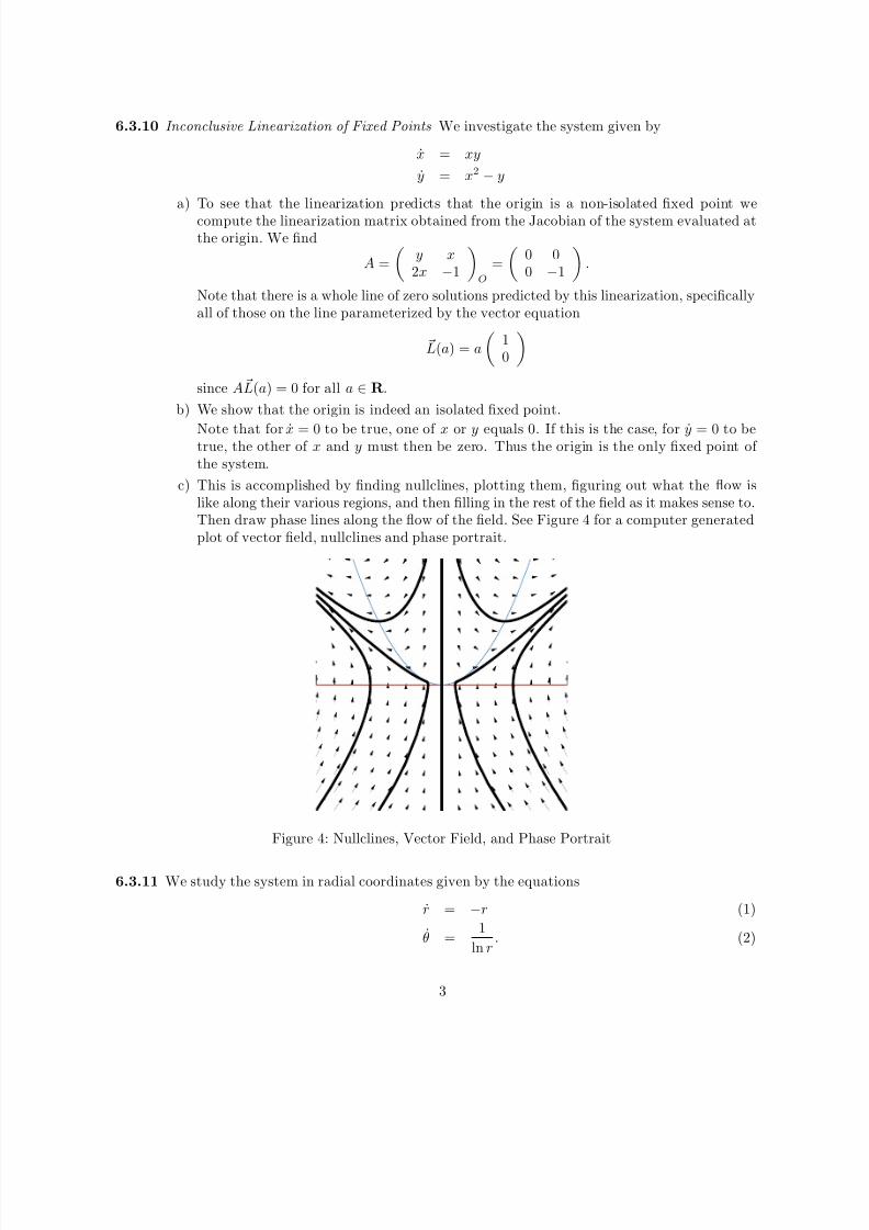
Figure 3: Nullclines, Vector Field, and Phase Portrait

x = xy − 1

y = x − y3

Setting things equal to zero, we find that the x-nullcline is y = 1/x and our y-nullcline isy = x1/3. Intersections occur at points (1, 1) and (−1, −1). To use linear analysis at thesepoints we compute the Jacobian and evaluate at our fixed points giving us the matrices

A =

1 11 −3

, B =

−1 −11 −3

for the fixed points (1, 1) and (−1, −1) respectively. We calculate the traces and determinantsto be T = −2 and D = −5 for (1, 1) and for (−1, −1) we have T = −4 and D = 4. This meansthat the former fixed point is a saddle and the latter is stable and somewhere in between aspiral and a sink. See Figure 3 for a plot of the vector field with nullclines and phase portrait.

2



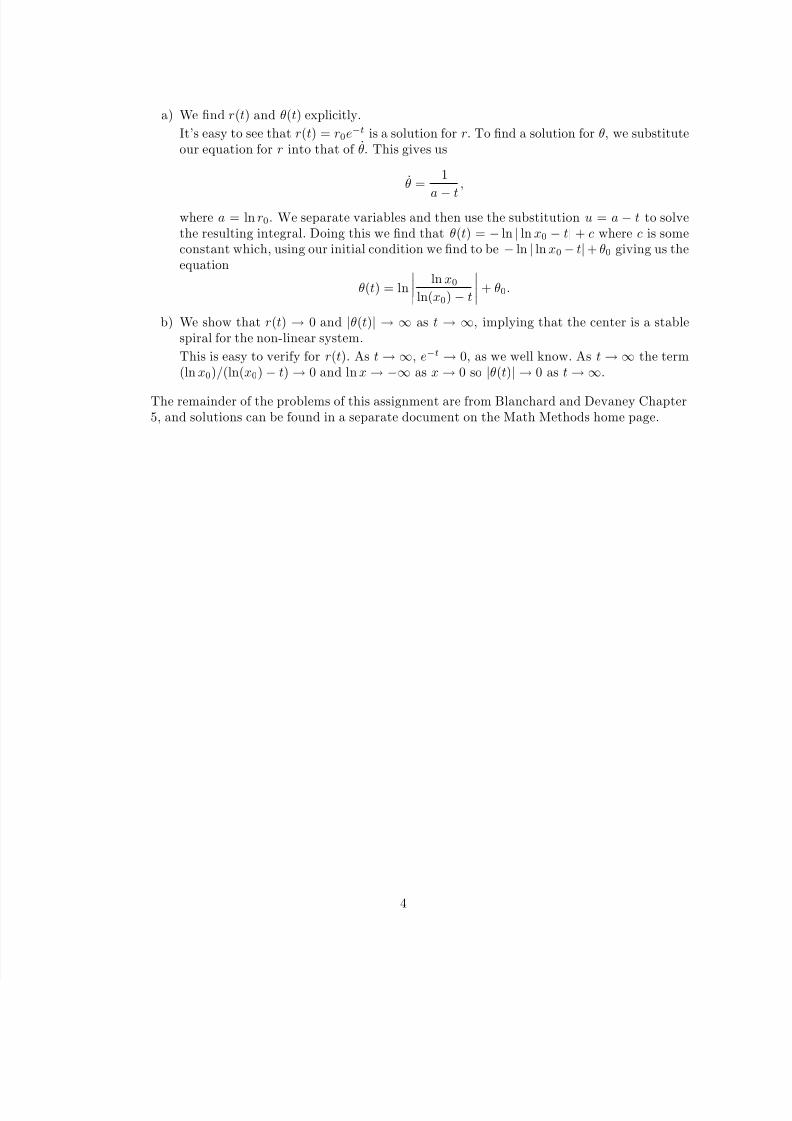
6.3.10 Inconclusive Linearization of Fixed Points We investigate the system given by

x = xy

y = x2 − y

a) To see that the linearization predicts that the origin is a non-isolated fixed point we

compute the linearization matrix obtained from the Jacobian of the system evaluated atthe origin. We find

A =

y x

2x −1

O

=

0 00 −1

.

Note that there is a whole line of zero solutions predicted by this linearization, specificallyall of those on the line parameterized by the vector equation

L(a) = a

10

since A L(a) = 0 for all a ∈ R.

b) We show that the origin is indeed an isolated fixed point.

Note that for x = 0 to be true, one of x or y equals 0. If this is the case, for y = 0 to betrue, the other of x and y must then be zero. Thus the origin is the only fixed point of the system.

c) This is accomplished by finding nullclines, plotting them, figuring out what the flow islike along their various regions, and then filling in the rest of the field as it makes sense to.Then draw phase lines along the flow of the field. See Figure 4 for a computer generatedplot of vector field, nullclines and phase portrait.

Figure 4: Nullclines, Vector Field, and Phase Portrait

6.3.11 We study the system in radial coordinates given by the equations

r = −r (1)

θ =1

ln r. (2)

3



a) We find r(t) and θ(t) explicitly.

It’s easy to see that r(t) = r0e−t is a solution for r. To find a solution for θ, we substituteour equation for r into that of θ. This gives us

θ =1

a − t

,

where a = ln r0. We separate variables and then use the substitution u = a − t to solvethe resulting integral. Doing this we find that θ(t) = − ln | ln x0 − t| + c where c is someconstant which, using our initial condition we find to be − ln | ln x0 − t| + θ0 giving us theequation

θ(t) = ln

ln x0

ln(x0) − t

+ θ0.

b) We show that r(t) → 0 and |θ(t)| → ∞ as t → ∞, implying that the center is a stablespiral for the non-linear system.

This is easy to verify for r(t). As t → ∞, e−t → 0, as we well know. As t → ∞ the term(ln x0)/(ln(x0) − t) → 0 and ln x → −∞ as x → 0 so |θ(t)| → 0 as t → ∞.

The remainder of the problems of this assignment are from Blanchard and Devaney Chapter5, and solutions can be found in a separate document on the Math Methods home page.

4

non-linear strogatz 4

Documents