optical co sensors for the investigation of the global
TRANSCRIPT

Dipl.
Optical CO2 Sensors for the
Zur Erlangung des akademischen Grades
„Doktorin der technischen Wissenschaften
Univ.-Prof. Dipl.
Institut für analytische Chemie und Lebensmittelchemie
Dipl.-Ing. Susanne Schutting, BSc.
Sensors for the Investigation of the Global Carbon Dioxide Cycle
DISSERTATION
Zur Erlangung des akademischen Grades
Doktorin der technischen Wissenschaften“
eingereicht an der
Technischen Universität Graz
Betreuer
Prof. Dipl.-Chem. Dr. rer.nat., Ingo Klimant
Institut für analytische Chemie und Lebensmittelchemie
Graz, Juli 2015
Investigation of the Global
“
nat., Ingo Klimant
Institut für analytische Chemie und Lebensmittelchemie


Dissertation S. Schutting
I
EIDESSTATTLICHE ERKLÄRUNG
Ich erkläre an Eides statt, dass ich die vorliegende Arbeit selbstständig verfasst, andere als die angegebenen Quellen/Hilfsmittel nicht benutzt, und die den benutzten Quellen wörtlich und inhaltlich entnommenen Stellen als solche kenntlich gemacht habe. Das in TUGRAZonline hochgeladene Textdokument ist mit der vorliegenden Dissertation identisch.
STATUTORY DECLARATION
I declare that I have authored this thesis independently, that I have not used other than the declared sources/resources and that I have explicitly marked all material which has been quoted either literally or by content from the used sources.
Datum/Date Unterschrift/Signature

Dissertation S. Schutting
II

Dissertation S. Schutting
III
Der genießt wahre Muße, der Zeit hat, den Zustand seiner Seele zu fördern.
& Es ist nicht wichtig, was Du betrachtest, sondern was Du siehst.
Henry David Thoreau

Dissertation S. Schutting
IV

Dissertation S. Schutting
V
Zusammenfassung
CO2 ist neben dem pH-Wert und Sauerstoff einer der wichtigsten Parameter für Umwelt und Industrie. Der Fokus dieses Projektes lag auf der Detektion von Kohlenstoffdioxid mittels optischen Plastik-Typ Sensoren, basierend auf pH-sensitiven Indikator-Farbstoffen. Derzeit hauptsächlich als Indikator verwendet wird 8-hydroxypyrene-1,3,6-trisulfonat (HPTS), jedoch besteht große Nachfrage an alternativen pH-sensitiven Farbstoffen mit verbesserten optischen Eigenschaften. In Kapitel 1 wird eine neue Farbstoffklasse, basierend auf Diketo-Pyrrolo-Pyrrolen (DPPs), vorgestellt. Diese DPP-Farbstoffe weisen hohe Quantenausbeuten, hohe pKs-Werte und gute Photostabilität auf. Diese Farbstoffe sind selbst-referenzierend und daher ideal für ratiometrische Messungen. Sensoren, die auf diesen DPPs basieren, können mittels Absorptions- oder Fluoreszenzmessungen ausgelesen werden. Durch unterschiedliche Startpigmente bzw. Substituenten können die dynamischen Bereiche der Sensoren angepasst werden. Kapitel 2 präsentiert einen hoch sensitiven CO2 Sensor, dessen Fluoreszenzeigenschaften mittels kommerziell erhältlicher RGB Kamera ausgelesen werden können. Eine zweite Klasse von pH-sensitiven Indikator-Farbstoffen wird in Kapitel 3 präsentiert. Die Verwendung dieser di-OH-aza-BODIPYs in optischen CO2 Sensoren ermöglicht die Messung im nahen Infrarot-Bereich (NIR). Diese ebenfalls selbst-referenzierenden Farbstoffe zeigen außergewöhnliche Photostabilität und hohe pKs-Werte, welche durch das Substitutionsmuster variiert werden können. Sensoren, welche darauf basieren, können mittels Absorption oder absorptionsmoduliertem Inner-Filter-Effekt ausgelesen werden. Kapitel 4 präsentiert den Prototypen eines Multifaser-Sensors (MuFO) mit 100 frei positionierbaren optischen Fasern für die CO2 Messung mit nur einer Anregungsquelle und Auslesung mit einer kommerziell erhältlichen Digitalkamera.

Dissertation S. Schutting
VI

Dissertation S. Schutting
VII
Abstract
Carbon dioxide is one of the most important parameters, besides pH and oxygen, for environmental and industrial monitoring. This project focused on optical plastic type sensors based on pH-sensitive indicator dyes for its detection. Up to now, state-of-the-art CO2 sensors are almost exclusively based on the pH-indicator 8-hydroxypyrene-1,3,6-trisulfonate (HPTS), but alternative self-referencing (dual-emitting) indicator dyes are highly desired. Chapter 1 presents a new class of indicator dyes based on diketo-pyrrolo-pyrroles (DPPs). Those dyes feature high fluorescence quantum yields, high pKa values and good photostability. Both the protonated and the deprotonated form are excitable in the blue part of the spectrum. Hence, those self-referenced dyes are excellently suitable for ratiometric measurements. Sensors based on those dyes can be read out via absorption or via fluorescence intensity. By diversifying the starting pigments and using different substituents the optical CO2 sensors were tuned to cover different dynamic ranges. A highly sensitive CO2 sensor was prepared and presented in chapter 2. Its fluorescence properties perfectly match the color channels of commercially available RGB cameras. Chapter 3 presents a second class of new indicator dyes based on BF2-chelated tetraarylazadipyrromethenes (aza-BODIPYs). The use of di-OH-aza-BODIPY dyes in carbon dioxide sensors enables measurements in the near infrared (NIR) region. These dyes show very high pKa values and excellent photostability. Carbon dioxide sensors based on those self-referenced aza-BODIPYs can be read out via absorption modulated inner filter effect. The dynamic ranges of the carbon dioxide sensors can be individually tuned by using di-OH-aza-BODIPY dyes with different substituents. Chapter 4 presents a prototype of a multiple fiber optics (MuFO) device with not one, but 100 freely positionable fibers excitable with one collective excitation source and read-out via imaging with a commercially available digital camera.

Dissertation S. Schutting
VIII

Dissertation S. Schutting
IX
Acknowledgement
THANK YOU, Ingo and Sergey. You were the most inspiring supervisors I could get. Your ideology, enthusiasm and passion for your work carried me along every single day and motivated me for new steps.
To the “old crew“- Klaus, Birgit, Lisi, Daniel, Babsi N., Tobi A. and B., Tijana, Torsten, Lego-Philipp, Gerda and Michela: Thank you for making me feel a member of this working group from the first day on. I enjoyed every discussion (serious or not), every lunch, every minute with you at this institute. Klaus, winning the first ACFC badminton cup with you as my partner was an honor. Birgit, your “Bloody Mary” was and will be the best of all! Lisi, not a single day is going by where I am not getting hungry at 11:30, thanks to you. Daniiiel, you are the perfect example of the loveliest confused professor in the world. Michela, with pleasure I learned the correct pronunciation of the word “comment” from you, especially because it took you at least 20 tries. Tobi A., thank you for drinking at least half of my drinks at the “Glühweinstand”. Tobi B., I love your cheese fondue, but eating it with friends like you makes it really special. Babsi N., your lab journals were the most accurate ones I have ever seen. Torsten, thank you for eating my raisin bread… without you I would have gained just too much weight. Tijana, your dry humor is unique and Philipp, I have never seen anybody before sitting on a table while having his diploma exam. And Gerda, your vocal and rhythmic arts were and always will be outstanding.
To the “new crew”- Mokka-Berni, blonde Berni, Ulli, Willy, David, Martin, Peter, Philipp (small), Heidi, Josef, Shiwen, Christoph, Eva, Rahel, Pia, Silvia, Anna and Larissa: Thank you all for accompanying me during my last years/months at the institute. Ulli, you were one of the most pleasant office mates I´ve ever had. Heidi, you are such a nice person… please, stay as you are. Special thanks to my beer-buddy David and my soccer-match-ticket-dealer Phips! Martin, the jungle camp would not have been so funny without you. Peter, my “favorite librarian” and social-activity-organizing-partner, thank you. Mokka-Berni, you are an excellent whisky-buddy, although you are mixing it sometimes with energy drinks. Josef, you are one of the most helpful and social people I know, thank you. Shiwen, do not forget your passport. Eva, I am sure you will make the best sticking-together CO2 sensor layers ever known. Blonde Berni, thanks for introducing me to the park house and for the delicious toast sessions. Willy, I have only two words for you: “mustard-colored jeans”… made my day. Christoph, I have never messed up so many “Quiz duell”-matches as I did while I was playing against you. Silvia, your sunny nature lightens up every single day. Rahel, I will miss your chocolate cake. Pia, thank you for your tireless dedication. Anna, I will miss the chats in the tram. ;) Larissa, you are one of the most adorable persons I´ve ever met.

Dissertation S. Schutting
X
To the “everlasting crew”- Eveline, Manuela, Iris, Erika, Marion: You are the heart of the institute. Please, never stop to be so helpful and dedicated. I have no words to describe how badly I will miss you.
Special thanks to Jan and Günter! From the MPI to the TU, I appreciated and enjoyed every discussion during work and chat during the breaks.
Last but not least, the “round-about crew”- Herbert, Helmar, Paul, Nina, Iris, Andrea, Sigi, Claudia, Erich, Barbara S. and Barbara P.-Z.: Herbert, I would have not been able to print anything without you. Helmar, Sigi, Iris and Nina, thank you for the puzzle evenings… although I think I will never go to Venice. Andrea, thank you for helping me during the lab course. Erich and Barbara S., I enjoyed your lectures. Your passion for food chemistry was absolutely infectious. Babsi P.-Z., thank you for organizing the dancing lessons. Paul and Claudia, you are so lovely people. Please, stay as you are.
Thank you all. You became friends, not only colleagues.
To the four most important persons in my life: Mum, Dad, Chri and Julia. I can not and don´t want to imagine how life would be without you. Thank you for the talks, the patience, the hours filled with love and happiness, for being as you are and for taking me as I am.

Dissertation S. Schutting
XI
Table of Contents
Theoretical Background ................................................................................................................ 1
Scope of the Thesis ................................................................................................................... 1
Carbon Dioxide and the Marine Ecosystem .............................................................................. 3
The Global Carbon Cycle ...................................................................................................... 3
Atmospheric Carbon Dioxide ............................................................................................... 3
Sources of Carbon Dioxide ................................................................................................... 4
Carbon Dioxide in the Ocean ................................................................................................ 4
Consequences of the CO2 Increase ........................................................................................ 7
Calculations ............................................................................................................................. 11
Conversion of ppm to µmol/l .............................................................................................. 12
Calculation of [CO2], [HCO3-] and [CO3
2-] ......................................................................... 13
Basics ...................................................................................................................................... 16
Absorption ........................................................................................................................... 16
Luminescence ...................................................................................................................... 16
Sensors ................................................................................................................................ 19
Optical Chemical Sensors ....................................................................................................... 21
Sensor Geometries .............................................................................................................. 22
Measurement Principles ...................................................................................................... 23
Materials .............................................................................................................................. 24
Matrices ............................................................................................................................... 25
Indicators ............................................................................................................................. 26
Carbon Dioxide Sensor Preparation .................................................................................... 30
Fields of Application - Optical Carbon Dioxide Sensors .................................................... 31
Comparison: Carbon Dioxide Detection Methods for Marine Applications .......................... 32
Introduction ......................................................................................................................... 32
Technical Comparison ........................................................................................................ 34
HydroC (CONTROS GmbH) .............................................................................................. 35
GasPro - Dissolved CO2 Probes (Sapienza University of Rome) ....................................... 37
Optical Chemical Sensors/ MuFO (Graz University of Technology) ................................. 39
Severinghaus CO2 Sensors – Microelectrode MI 720 (Microelectrodes Inc.) .................... 41
Experiences from Users ...................................................................................................... 44
Results - Overview ...................................................................................................................... 47
Chapter 1 - Diketo-Pyrrolo-Pyrrole Dyes as New Colorimetric and Fluorescent pH Indicators for Optical Carbon Dioxide Sensors .................................................................. 47

Dissertation S. Schutting
XII
Chapter 2 - New Highly Fluorescent pH Indicator for Ratiometric RGB Imaging of pCO2 ............................................................................................................................................. 47
Chapter 3 - NIR Optical Carbon Dioxide Sensors Based on Highly Photostable Dihydroxy-aza-BODIPY Dyes .............................................................................................................. 47
Chapter 4 - Multi-Branched Optical Carbon Dioxide Sensors for Marine Applications .... 48
Chapter 1 ..................................................................................................................................... 49
Scope of this chapter ............................................................................................................... 49
Diketo-Pyrrolo-Pyrrole Dyes as New Colorimetric and Fluorescent pH Indicators for Optical Carbon Dioxide Sensors .............................................................................................................. 51
Introduction ............................................................................................................................. 51
Experimental ........................................................................................................................... 53
Materials. ............................................................................................................................. 53
Synthesis of 3,6-bis[4´(3´)-disulfo-1,1´-biphenyl-4-yl]-2,5-dihydropyrrolo[3,4-c]pyrrole-1,4-dione dipotassium salt (1). ............................................................................................ 54
Synthesis of 3,6-bis[4´-bis(2-ethylhexyl)sulfonylamide-1,1´-biphenyl-4-yl]-2,5-dihydropyrrolo[3,4-c]pyrrole-1,4-dione (2). ....................................................................... 54
Synthesis of 3-(phenyl)-6-(4-bis(2-ethylhexyl)sulfonylamide-phenyl)-2,5-dihydropyrrolo[3,4-c]pyrrole-1,4-dione (3) and 3,6-bis[4-bis(2-ethylhexyl)sulfonylamide-phenyl]-2,5-dihydropyrrolo[3,4-c]pyrrole-1,4-dione (4)..................................................... 55
Preparation of the Sensing Foils. ......................................................................................... 56
Methods. .............................................................................................................................. 56
Results and Discussion ............................................................................................................ 58
Synthesis. ............................................................................................................................. 58
Properties of the Disulfonate 1. ........................................................................................... 59
Photophysical Properties of the Sulfonamides. ................................................................... 60
Photostability. ...................................................................................................................... 62
Carbon Dioxide Sensors. ..................................................................................................... 63
Comparison of the Optical and Sensing Properties with State-of-the-art Sensors. ............. 66
Sensor Response Times and Reproducibility. ..................................................................... 68
Conclusions ............................................................................................................................. 69
Acknowledgements ................................................................................................................. 70
Supporting Information ........................................................................................................... 71
Chapter 2 ..................................................................................................................................... 85
Scope of this chapter ............................................................................................................... 85
New Highly Fluorescent pH Indicator for Ratiometric RGB Imaging of pCO2 ......................... 87
Introduction ............................................................................................................................. 87
Experimental Details ............................................................................................................... 89

Dissertation S. Schutting
XIII
Materials .............................................................................................................................. 89
Synthesis of 2-hydro-5-tert-butylbenzyl-3,6-bis(4-tert-butyl-phenyl)-pyrrolo[3,4-c]pyrrole-1,4-dione (DPPtBu3) ........................................................................................................... 89
Preparation of the Planar Optodes ....................................................................................... 90
Methods ............................................................................................................................... 90
Results and Discussion ............................................................................................................ 91
Synthesis ............................................................................................................................. 91
Photophysical Properties ..................................................................................................... 92
Carbon Dioxide Sensors ...................................................................................................... 94
Photostability ...................................................................................................................... 97
RGB Imaging ...................................................................................................................... 98
Conclusions ............................................................................................................................. 99
Acknowledgments ................................................................................................................... 99
Supporting Information ......................................................................................................... 100
Chapter 3 ................................................................................................................................... 103
Scope of this chapter ............................................................................................................. 103
NIR Optical Carbon Dioxide Sensors Based on Highly Photostable Dihydroxy-aza-BODIPY Dyes .......................................................................................................................................... 105
Introduction ........................................................................................................................... 105
Experimental ......................................................................................................................... 107
Materials ............................................................................................................................ 107
Synthesis of 3,7-bis(4-butoxyphenyl)-5,5-difluoro-1,9-diphenyl-5H-4λ4,5λ4-dipyrrolo[1,2-c:2',1'-ƒ][1,3,5,2]triazaborinine (di-butoxy-complex) ....................................................... 108
Synthesis of 4,4'-(5,5-difluoro-1,9-diphenyl-5H-4λ4,5λ4-dipyrrolo[1,2-c:2',1'-ƒ][1,3,5,2]triazaborinine-3,7-diyl)bis(2-chlorophenol) (di-Cl-di-OH-complex) .............. 109
Synthesis of 4,4'-(5,5-difluoro-1,9-diphenyl-5H-4λ4,5λ4-dipyrrolo[1,2-c:2',1'-ƒ][1,3,5,2]triazaborinine-3,7-diyl)bis(3-fluorophenol) (di-F-di-OH-complex) ................ 110
Synthesis of 4,4'-(5,5-difluoro-1,9-diphenyl-5H-4λ4,5λ4-dipyrrolo[1,2-c:2',1'-ƒ][1,3,5,2]triazaborinine-3,7-diyl)diphenol (di-OH-complex).......................................... 111
Synthesis of the 4,4'-(5,5-difluoro-1,9-diphenyl-5H-4λ4,5λ4-dipyrrolo[1,2-c:2',1'-ƒ][1,3,5,2]triazaborinine-3,7-diyl)bis(2-methylphenol) (di-CH3-di-OH-complex) .......... 111
Staining of PS-Microparticles ........................................................................................... 112
Sensor Preparation ............................................................................................................ 112
Methods ............................................................................................................................. 113
Results and Discussion .......................................................................................................... 114
Synthesis ........................................................................................................................... 114
Photophysical Properties ................................................................................................... 115
Dissertation S. Schutting
XIV
Carbon Dioxide Sensors .................................................................................................... 117
Luminescence-based Ratiometric Read-out using IFE (Inner-Filter Effect) based Sensors ........................................................................................................................................... 121
Carbon Dioxide Production/Consumption of a Hebe Plant ............................................... 122
Conclusion ............................................................................................................................. 124
Acknowledgment .................................................................................................................. 124
Supporting Information ......................................................................................................... 125
Chapter 4 ................................................................................................................................... 137
Scope of this chapter ............................................................................................................. 137
Multi-Branched Optical Carbon Dioxide Sensors for Marine Applications ............................. 139
Introduction ........................................................................................................................... 139
Experimental ......................................................................................................................... 140
Materials ............................................................................................................................ 140
Sensing Chemistry ............................................................................................................. 142
Methods ............................................................................................................................. 143
Results and Discussion .......................................................................................................... 144
Principle ............................................................................................................................ 144
Sensing Chemistry ............................................................................................................. 145
Calibration and Temperature Dependence ........................................................................ 147
LOD and Response Time .................................................................................................. 149
Carbon Dioxide Dynamics at Panarea Island (Sicily, Italy) .............................................. 149
Conclusion and Outlook ........................................................................................................ 152
Acknowledgment .................................................................................................................. 153
Supporting Information ......................................................................................................... 154
Conclusion and Outlook ............................................................................................................ 161
References ................................................................................................................................. 165
Appendix A ............................................................................................................................... 177
List of Figures ....................................................................................................................... 177
List of Schemes ..................................................................................................................... 179
List of Tables ......................................................................................................................... 179
Appendix B – Curriculum Vitae ............................................................................................... 180

Theoretical Background S. Schutting
1
Theoretical Background
Scope of the Thesis
Carbon dioxide is one of the most important parameters concerning different processes
in nature, science and industry. Whereas by oxygen monitoring only aerobic activities
can be observed, also anaerobic activities are observeable by monitoring carbon
dioxide. 98% of the worlds carbon dioxide deposits are stored in the deeper oceans. The
increasing carbon dioxide level causes problems like global warming (greenhouse
effect) or the acidification of the oceans. The latter causes not only a lowered pH, but
also several consequences on the oceans flora and fauna.
For marine science the demands on detection methods can range from the atmospheric
pCO2 level (0.04 kPa ≈ 400 µatm in the gas phase ≈ 11.6 µmol/l in seawater at 298.15
K) to very high pCO2 values, e.g. in the vicinity of volcanic seeps. Especially for field
experiments where time, equipment and staff are limited, it is important that the method
is easily adaptable to the respective conditions of the experiment and that it gives as
much simultaneous information as possible concerning spatial and temporal distribution
of the analyte concentration.
Routine detection techniques of CO2 like infrared (IR) spectroscopy, gas
chromatography (GC) or the Severinghaus electrode are well established, but suffer
from different drawbacks. Although several new concepts of chemosensors for the
detection of CO2 were published in recent years, optical plastic type sensors are the
most common ones. These sensors consist of a pH-sensitive indicator dye and a base
(acting as lipophilic buffer), embedded in a polymer matrix and represent a promising
alternative to the known routine techniques. The dynamic range of the CO2 sensors can
be tuned by varying the pKa value of the indicator dye, by using different bases or
matrix materials. Up to now, state-of-the-art CO2 sensors are almost exclusively based
on the fluorescent pH-indicator 8-hydroxypyrene-1,3,6-trisulfonate (HPTS), the base
tetraoctyl ammonium hydroxide (TOAOH) and ethyl cellulose as matrix material.
Alternative materials, especially self-referencing (dual-emitting) indicators with spectral
properties in the visible range, as well as in the NIR region are presented in this thesis.

Theoretical Background S. Schutting
2

Theoretical Background S. Schutting
3
Carbon Dioxide and the Marine Ecosystem
The Global Carbon Cycle
The global carbon cycle describes the exchange of carbon (as CO2, CO, CH4, organic
matter, fossil fuels, etc.) between the reservoirs, which are acting either as source
(release of carbon) or sink (uptake of carbon). The major reservoirs of carbon on earth
are: the atmosphere, the oceans and the terrestrial system (also: the lithosphere, the
aquatic biosphere and fossil fuels),1,2 where the largest and dominating reservoir – the
oceans – and the terrestrial system are linked via the atmosphere.3
Figure I shows an overview of the carbon reservoirs, their capacities and the fluxes and
rates inbetween. Especially the anthropogenic impact has left a big footprint on the
global carbon cycle during the last two to three centuries. The development of new
machines and technologies during the industrial revolution brought a strong increase in
carbon fluxes, in particular concerning carbon dioxide and methane.
Figure I. Global carbon cycle.4 Red: anthropogenic fluxes; Black: natural fluxes (before industrial revolution).
Atmospheric Carbon Dioxide
One of the strongest leverage effects to the global carbon cycle is the atmospheric CO2
level and its interactions with the cycle. Its changing rate is highly affected by
anthropogenic influences, biogeochemical and climatological processes.1 Here, the main
focus will be the balance between atmospheric carbon dioxide and the ocean, which is
the major sink for CO2.3

Theoretical Background S. Schutting
4
Sources of Carbon Dioxide
As mentioned before, the carbon reservoirs (either sink or source) are linked to each
other and exchange carbon and/or carbon dioxide. However, there are several big
sources – natural or anthropogenic - of carbon dioxide. Especially during the last two
centuries the anthropogenic sources had a high impact on earth´s atmosphere pCO2
level:
- Natural sources: The biggest (short-term) natural sources for carbon dioxide are
volcanic carbon dioxide seeps,5 total global emission of CO2 from soils,6 decay
of organic matter, heterotrophic respiration and natural fires.7 Ice core analysis
showed that the atmospheric CO2 level altered several times between 180 and
280 µatm before the industrial revolution in the 19th century.8 Therefore, even
for short-term exposures with high levels of carbon dioxide, such as during
volcanic activities, no significant long-term effects were recordable.
- Anthropogenic sources: The level of atmospheric CO2 is strongly affected by
human activities. In the 18th/19th century, when industry started to introduce
more efficient manufacturing machines and processes, the anthropogenic impact
on the atmospheric carbon dioxide level increased rapidly and led to a sharp
increase of atmospheric CO2 up to more than 360 µatm.8,9 Today, the major
sources for anthropogenic CO2 are: anthropogenic deforestation,4,10,11 iron and
steel production,12 agricultural economy,2 burning fossil-fuels2,4,11 and cement-
manufacturing emissions.4,13 All these sources transport carbon from the
terrestrial reservoir to the atmosphere as carbon dioxide and therefore affect the
carbon dioxide level of the ocean.
Carbon Dioxide in the Ocean
CO2 is exchanged across the ocean-atmosphere interface, even forced by strong and
continuous winds over the ocean surface.2 Thus, the atmospheric carbon dioxide level is
in a dynamic equilibrium with the surface layer of the oceans, which is influenced by
different processes, such as upwelling (nutrient-rich upward current from the deep sea),
downwelling (nutrient-rich downward current to the deep sea), vertical diffusion,
advection and gravitational drift of biogenic materials.2 The major driving forces are:

Theoretical Background S. Schutting
5
- Chemical processes:
Dissolution in water (figure II): After CO2 is dissolved in water, it forms carbonic
acid H2CO3. This formation is the slowest step in these equilibria series compared
to the ionization of the carbonic acid, which is much faster and yields bicarbonate
ions and protons.14 Bicarbonate is the dominant species. Firstly, bicarbonate can
dissociate to carbonate ions and protons, but carbonate ions can also be
reprotonated by the protons build during the dissociation of carbonic acid. In this
case the concentration of carbonate is lowered again.
The equilibria between the three species – bicarbonate ions ~90%, carbonate ions
~10% and unionized dissolved carbon dioxide <1% at a pH of ~8.29,14 – are in
balance with other acid-base equilibria (e.g. boric acid) and the pH value of the
ocean. Although it seems sometimes, as the pH is influencing the equilibria of the
carbonate cycle, the opposite is the truth – the carbonate system acts as buffer of
the ocean. The carbonate equilibria, the pKa values for carbonic acid, the relation
to pH and to the boric acid equilibrium can also be seen in the Bjerrum plot in
figure II (right).15
The sum of the concentrations of unionized dissolved carbon dioxide, HCO3- and
CO32- is also known as the (total) dissolved inorganic carbon CT and is only ~2
mmol/kg (surface layer, North Atlantic).14,16
Carbon dioxide shows increased solubility in cold seawater with higher density
and salinity. When the water is sinking down, the carbon dioxide is transported to
deeper depths.
Figure II. Left: Reactions of carbon dioxide in water.14,16 Right: the Bjerrum plot15 (DIC = 2.1 mmol/kg, S = 35, T = 25°C). Here, pKa1 and pKa2 of carbonic acid are 5.86 and 8.92, respectively.
Theoretical Background S. Schutting
6
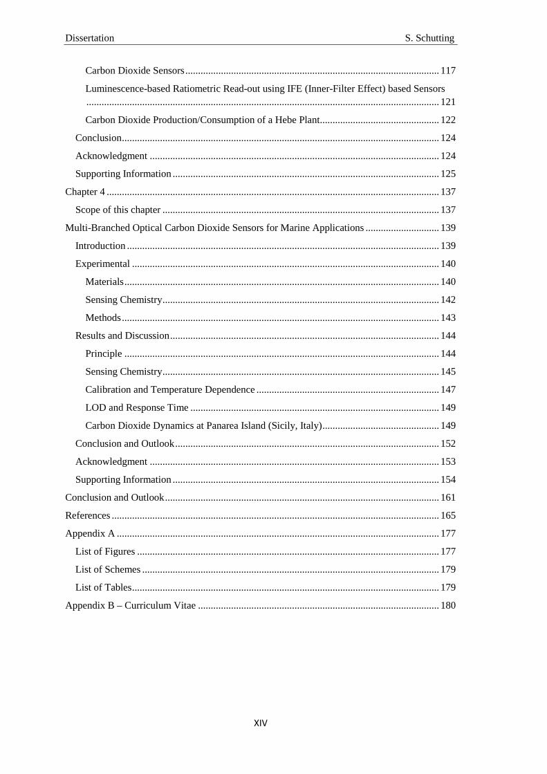
- Biological processes (figure III):
The organic biological pump:2 CO2 uptake is also forced by biological processes,
such as the carbon dioxide consumption during phytoplankton photosynthesis in
depths of the ocean where light can still penetrate. Inorganic compounds and
organic matter are produced. This is also called primary production.2 The
products are then transported (via sinking, advection or mixing) to the deep sea,
where they re-mineralize or are decomposed by bacteria. The transfer rate from
the surface layer to the deep sea is called new production.2 Via upwelling CO2 is
partially transferred back to the surface layer of the ocean.
The carbonate pump1,17,18 is a special case of the organic biological pump. CaCO3
shells can be built by different planktonic species. Afterwards they sink to the
seafloor (gravitational drift of biogenic materials)2 and can re-dissolve, because
CaCO3 shows increased solubility in colder water and under higher pressure.9
Again, via upwelling CO2 is only partially transferred back to the surface layer of
the ocean. Thus, CO32- is “pumped” to deeper layers of the ocean. The three main
producers for CaCO3 are coccolithophores, foraminifera and euthecosomatous
pteropods,9 whereas 23-56% of the total open marine CaCO3 flux are covered by
planktonic foraminifera.18
Figure III. Scheme of the responsible biological processes for the uptake/storage of carbon dioxide in the ocean.
The upper layer of the ocean is defined as an almost homogeneous layer of seawater,
which shows only small changes in temperature and density in dependence to the depth.
The depth of this layer is often called isothermal layer depth (ILD) in case of limitation

Theoretical Background S. Schutting
7
by temperature changes or mixed layer depth (MLD) in case of limitation by density
changes.19
The above described processes are displaying the major paths of storing carbon/ carbon
dioxide in the deeper ocean. Thus, the lower part of the oceans is enriched with CO2 and
is overlaid with the upper layer containing less carbon dioxide. Therefore, the upper
layer is acting as a barrier between the atmosphere and the lower ocean layer3 and CO2
from the lower layer can not re-equlibrate with the atmosphere. Nowadays, there are
~720 Gt of carbon dioxide in the atmosphere, but more than the fiftyfold in the lower
ocean layer.1
More or less one third of the anthropogenic produced atmospheric carbon dioxide is
absorbed by the oceans13 and can there be stored in different ways:2
- As dissolved inorganic carbon (DIC or CT): the sum of dissolved CO2, carbonic
acid, bicarbonate ions and carbonate ions
- As dissolved organic carbon (DOC): small and large molecules (simply
hydrocarbons to polysaccharides)20
- As particulate organic carbon (POC): the sum of living organisms and fragments
of dead plants and animals
Consequences of the CO2 Increase
The level of atmospheric CO2 is expected to be 730 µatm to over 1000 µatm by the end
of 2100, which would lead to a drop of the oceans pH of 0.3 to 0.4 units.21,22 Influences
of the elevated pCO2 will thus be definitely amplified and are discussed in this section.
As carbon dioxide is the most important greenhouse gas besides methane, tropospheric
ozone, nitrous oxid and chlorofluorocarbons (CFCs), it is a decisive parameter
concerning global warming, also known as greenhouse effect.11,23,24
Here, solar infrared radiation is needed for many natural processes and is absorbed by
the earth’s atmosphere and surface. To keep the energy and/or heat balance at
equilibrium thermal radiation is re-emitted by the earth’s surface. Molecules, such as
carbon dioxide, absorb the thermal radiation and are therefore responsible for the warm
up of the first layer of the atmosphere – the troposphere (10-15 km), where the
Theoretical Background S. Schutting
8
greenhouse effect mainly happens.11
Global warming can cause various effects, e.g. melting of ice caps, that causes a noise
increase in the oceans and a rise of the sea level.3,25 Tropical forests for example tend to
increase the respiration rate, decrease the growth and show increased natural fire risk.7
This again leads to higher levels of atmospheric carbon dioxide, which is only partially
compensated by the ocean reservoir.
The likelihood of extreme events like floodings or extended droughts is enhanced by
global climate change.26 In consequence, natural or man-made water reservoirs are
increasingly stressed. They show higher temperature, increased evaporation, decreased
precipitation and up-concentration related eutrophication.26,27 Additionally, the
magnitude of high and low water level is influenced by agricultural economy, as more
water is needed during dry periods.28 These affects can lead to a dramatic decline of the
reservoirs or even to their disappearance.
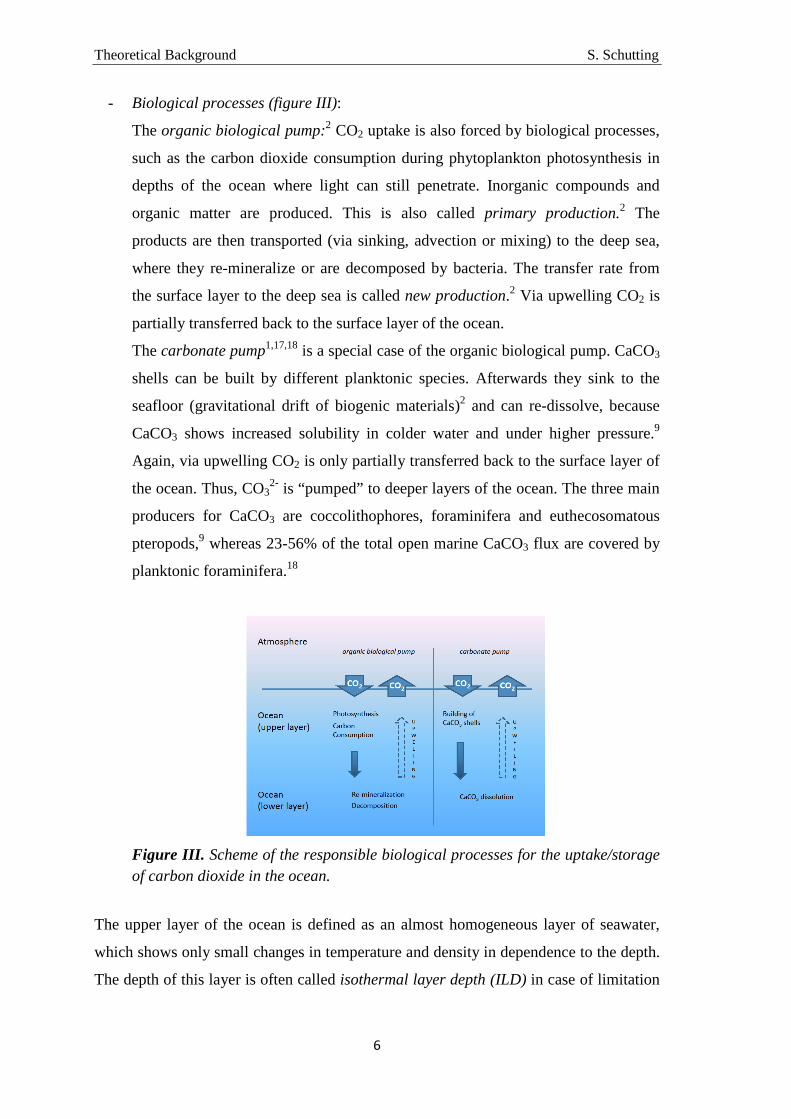
CO2 enhanced uptake by the oceans leads to an increase of the TC and a correlated
increase in proton concentration.9 This carbon dioxide increase leading to a lowered pH
value is also called ocean acidification or seawater acidification.9 A widely known
factor to express the CO2-buffering via pH lowering is the Revelle factor (also buffer
factor) Rf.15 It describes the uptake capacity of carbon dioxide in the oceans when the
level of atmospheric CO2 rises and was well explained by Zeebe and Wolf-Gladrow.15
�� =������ �� ������
���
�����������
Concerning the flora and fauna, on the one hand, the acidification causes a decrease of
the saturation of CaCO3 and therefore has an impact on the calcification rates.9 This
means, that – as mentioned before – the uptake of CO2 lowers the concentration of
carbonate ions. Calcifying species like corals, molluscs, echinoderms and crustaceans9
build their skeletons and shells using Ca2+ and CO32- ions. As the Ca2+ concentration in
seawater is almost constant (although depending on the salinity), the limiting factor for
these species is the concentration of carbonate ions.9 Hence, calcifying species are
increasingly restricted in building their CaCO3 shells. Additionally, if there are less
Theoretical Background S. Schutting
9
shells built, less CO32- is transported to the deeper oceans and therefore, stays in the
upper ocean layer and in the atmosphere.
The acidification affects the acid-base physiology of the extracellular body fluids of the
animals, e.g. blood, haemolymph or coelomic fluid,29 and lowers the pH value of the
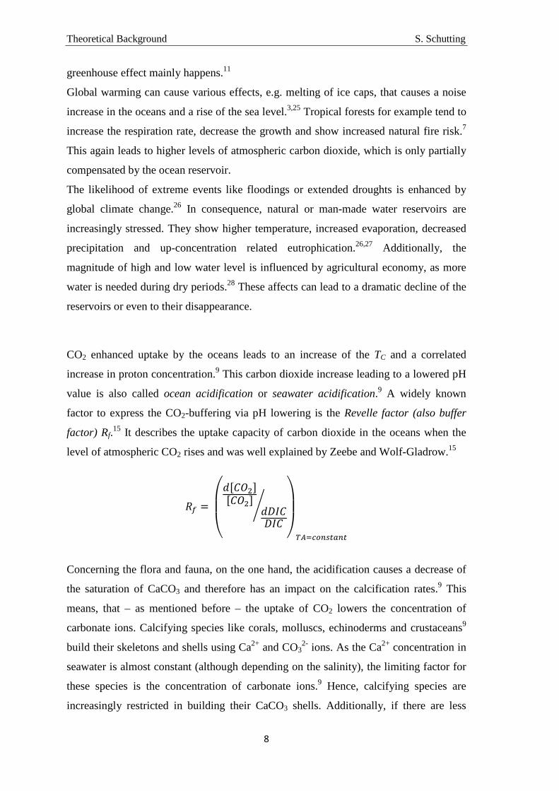
blood. An increase of pCO2 in the blood is also called hypercapnia.9 As a consequence
the oxygen binding of some species is influenced negatively. This relation is descriped
by the Bohr coefficient CB (P50 = pO2 required to achieve 50% oxygen saturation of the
respiratory protein).9,30
� =∆� !"#$∆%&
Some species are able to suppress their metabolism to counteract low pH or high pCO2
values by reducing their protein synthesis.9 Although reversible at short-term exposure,
this affects the growth and reproductive potential in a negative way and is even worse at
long-term exposure. Hence, the reproducibility is restricted and leads sooner or later to a
decrease of the diversity of species.
Fishes are affected concerning their olfactory senses. For example, several coral reef
fishes get susceptible for predation, as well as predator fishes change their hunting
behavior.21,31 Even fish species, e.g. cod, which show CO2 independent behavior to the
smell of predatory or non-predatory fishes, may e.g. change their movements.32
According to de Baar and Stoll3 the uptake of CO2 in the oceans will be affected, as the
chemical dissolution processes will decrease with rising carbon dioxide level and the
biological processes (carbonate pump, etc.) will probably stay constant or show a slight
increase.
Although there are more disadvantages, also the advantages of the increasing CO2 level
should be mentioned, e.g. a CO2 related decrease of ammonia33 or seagrass that shows
increased photosynthetic rates and net productivity and thus, features great affinity to
areas with elevated pCO2 values.34,35
However, one should be aware of the fact that a dramatic decrease of the human caused
global CO2 emissions will not automatically end in an immediate drop of the
atmospheric carbon dioxide level. The capacity of the oceans might be as high to take
up a big part of the anthropogenic carbon dioxide, but this might take a long time. De
Baar and Stoll already discussed this problem in 1992: “Only after several thousands to

Theoretical Background S. Schutting
10
millions of years most, but not all, of the fossil fuel CO2 will be taken up by the
oceans.”3
So called carbon (dioxide) capture and storage (CCS) strategies are under development,
but not yet fully investigated concerning their long-term consequences. A definition of
CCS was provided by a special report – IPCC Special Report on Carbon Dioxide
Capture and Storage – on this topic of the Intergovernmental Panel on Climate Change
(IPCC): “Carbon dioxide (CO2) capture and storage (CCS) is a process consisting of
the separation of CO2 from industrial and energy-related sources, transport to a
storage location and long-term isolation from the atmosphere.”
One of these strategies would be the sub-seabed geological storage of carbon dioxide.
Here, carbon dioxide is collected and pumped into sub-seabed geological formations,
e.g. the porous formations remaining from oil drilling rigs. Deep sea injection strategies
were already discussed in 1992 from de Baar and Stoll.3 Here, CO2 is collected and
pumped into deeper ocean layers. However, scientists are still investigating the
consequences, if carbon dioxide erupts quickly due to geological formation fractures or
if it is transported back to the upper ocean layer and the atmosphere.

Theoretical Background S. Schutting
11
Calculations
It was already mentioned, that although the upper layer of the ocean is in a dynamic
equilibrium with the atmosphere, the biggest part of the carbon dioxide is stored in the
deeper layers of the ocean. Numerical, almost 98% of the carbon dioxide are stored in
the ocean, due to its further reactions in water.15 The carbonate system is influenced by
various factors, such as temperature, salinity or other species in the seawater that show
acid-base equilibria, e.g. boric acid (table I). The focus of this thesis is the detection of
carbon dioxide in seawater, but not only the concentration of dissolved carbon dioxide
is of great interest, but also the concentrations of HCO3- and CO3
2- ions are. The
equations to describe and calculate the carbonate system are well collected and
explained by Zeebe and Wolf-Gladrow in CO2 in Seawater: Equilibrium, Kinetics,
Isotopes.15 The following section is an extraction of this book and should give an
overview of how to calculate the ratios between the species of the carbonate system –
dissolved CO2, HCO3- and CO3
2-.
Table I. Averaged standard chemical composition of seawater at a salinity of 35.15,16
Ion g/kg mol/kg Cl- 19.3524 0.54586 Na+ 10.7837 0.46906
Mg2+ 1.2837 0.05282 SO4
2- 2.7123 0.02824 Ca2+ 0.4121 0.01028 K+ 0.3991 0.01021
CO2 0.0004 0.00001 HCO3
- 0.1080 0.00177 CO3
2- 0.0156 0.00026 B(OH)3 0.0198 0.00032 B(OH)4
- 0.0079 0.00010 Br- 0.0673 0.00084 Sr2+ 0.0079 0.00009 F- 0.0013 0.00007
OH- 0.0002 0.00001 ∑ 35.1717 1.11994
Ionic Strength 0.69734
Theoretical Background S. Schutting
12
Initially, a few definitions have to be mentioned:
The sum of the species of the carbonate system (dissolved CO2 incl. H2CO3, HCO3- and
CO32-) is called dissolved inorganic carbon, shortly DIC. Other abbreviations are ∑CO2,
TCO2 or CT. This terms focus on the carbon.
DIC = [CO2] + [HCO3-] + [CO3
2-]
The carbonate alkalinity (CA) focuses on the charges, is part of the total alkalinity and
is defined as:
CA = [HCO3-] + 2*[CO3
2-]
The total alkalinity (TA or AT) also focuses on the charges and includes also boron
compounds and others:
TA = [HCO3-] + 2*[CO3
2-] + [B(OH)4-] + [OH-] – [H+] + minor components
In total, the carbonate system can be calculated via six variables: DIC, CA, [H+], [CO2],
[HCO3-] and [CO3
2-], where two have to be known to enable the calculation of the
remaining four.
Conversion of ppm to µmol/l
To express the concentration of carbon dioxide several units are used. Companies are
mostly using the unit ppm, where one has to define which ppm is meant: mg CO2/l or
volume percent*10000 at 1 atmosphere (sometimes ppmv). Scientists usually prefer
molarity units, e.g. mol/l, mmol/l or µmol/l.
The conversion of ppm (volume percent*10000 at 1 atmosphere) to molarity can be
carried out by using Henrys law, where the molarity of a dissolved gas is calculated
from its partial pressure in the gas phase above the solution.
'�( =)* ∙ ,
Where f Fugacity of the substance [atm]
caq Concentration of the substance in solution [mol/kg]
kH Henry constant [mol/kg*atm]

Theoretical Background S. Schutting
13
The Henry constant shows significant temperature dependence. Zeebe and Wolf-
Gladrow recommend the calculation of Weiss (1974):15
ln )* =9345.176 − 60.2409 + 23.3585 ∙ ln = 6100> + ?∙ @0.023517 − 0.00023656 ∙ 6 + 0.0047036 ∙ = 6100>
�A Where kH Henry constant dependent on the temperature [mol/kg*atm]
T Temperature [K]
S Salinity; ~35 g salt/kg seawater (see table I) [g/kg]
The molarity of carbon dioxide at different temperatures will be calculated as an
example. The results are shown in table II. The atmospheric level of carbon dioxide is
~400 ppm, which is equal to ~400 µatm (400 ppm = 400 µatm = 0.0004 atm). As the
result of the Henrys law calculation gives mol/kg, this unit is converted to mol/l
considering the density of seawater, being higher than that of freshwater.
Table II. Temperatures from 20-30°C, the respective Henry constants, the carbon dioxide concentration in µmol/kg and µg/kg, the seawater density and the CO2 concentrations in µmol/l and µg/l, calculated from the atmospheric level of CO2 (0.0004 atm) at a salinity of 35.1717.
Temperature
[°C] [K]
ln kH
kH
[mol/kg*atm]
Seawater Density
[g/l]
c(CO2)aq
[µmol/l]
c(CO2)aq
[µg/l]
20.00 293.15 -3.430 0.03238 1024.8 13.27 584.1 25.00 298.15 -3.563 0.02837 1023.3 11.61 511.0 30.00 303.15 -3.683 0.02515 1021.7 10.28 452.3
Calculation of [CO2], [HCO 3-] and [CO3
2-]
The equilibria between the species [CO2], [HCO3-] and [CO3
2-] show two equilibrium
constants K1 and K2, also called first and second dissociation constants of carbonic acid.
BC = &�DE ∙ &F ��
B� = �D�E ∙ &F &�DE
Theoretical Background S. Schutting
14
There are several equations for the calculation of K1 and K2. Zeebe and Wolf-Gladrow
recommend the equations from Roy et al.:16
lnBC = 2.83655 − 2307.12666 − 1.5529413 ∙ �GH6I − =0.207608410 + 4.04846 >∙ √? + 0.0846834 ∙ ? − 0.00654208 ∙ K?D + �GH1 − 0.001005 ∙ ?I
ln B� =−9.226508 −3351.61066 − 0.2005743 ∙ lnH6I− =0.106901773 + 23.97226 > ∙ √? + 0.1130822 ∙ ? − 0.00846934∙ K?D + �GH1 − 0.001005 ∙ ?I
Where K1,2 Equilibrium constants (1st and 2nd dissociation constants of carbonic acid)
T Temperature [K]
S Salinity; ~35 g salt/kg seawater (see table I) [g/kg]
For a salinity of ~35 and a temperature of 25°C (298.15 K) lnK1 should give -13.4847
and lnK2 should give -20.5504.
As mentioned, by knowing two variables of the carbonate system, the remaining four
can be calculated. Here, the calculation of the carbonate system is shown based on
known pH and CO2 concentration (from direct measurement).
%& =−� !&F �� = �� ∙ =1 + BC&F + BC ∙ B�&F � >
Where DIC dissolved inorganic carbon [mol/l]
[H+] proton concentration calculated from the measured pH [mol/l]
[CO2] concentration of dissolved CO2, incl. [H2CO3] [mol/l]
Using the DIC, the proton concentration and the equilibrium constants, the
concentrations of HCO3- and CO3
2- and the carbonate alkalinity can be calculated.
Theoretical Background S. Schutting
15
&�DE = ��=1 + &F BC + B�&F >
�D�E = ��=1 + &F B� + &F �BC ∙ B�>
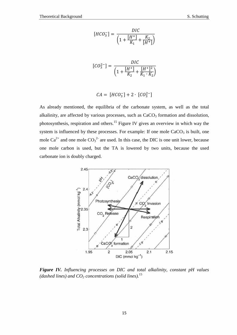
L = &�DE + 2 ∙ �D�E As already mentioned, the equilibria of the carbonate system, as well as the total
alkalinity, are affected by various processes, such as CaCO3 formation and dissolution,
photosynthesis, respiration and others.15 Figure IV gives an overview in which way the
system is influenced by these processes. For example: If one mole CaCO3 is built, one
mole Ca2+ and one mole CO32- are used. In this case, the DIC is one unit lower, because
one mole carbon is used, but the TA is lowered by two units, because the used
carbonate ion is doubly charged.
Figure IV. Influencing processes on DIC and total alkalinity, constant pH values (dashed lines) and CO2 concentrations (solid lines).15
Theoretical Background S. Schutting
16
Basics
Absorption
If a molecule absorbs photons, an electron can undergo a transition from the ground
state to an excited state, this means a transition from the highest occupied molecule
orbital to the lowest unoccupied orbital (HOMO → LUMO). There are several
electronic transitions, which can be lined up according to their energy:36
n → π* < π → π* < n → σ* < σ → π* < σ → σ*
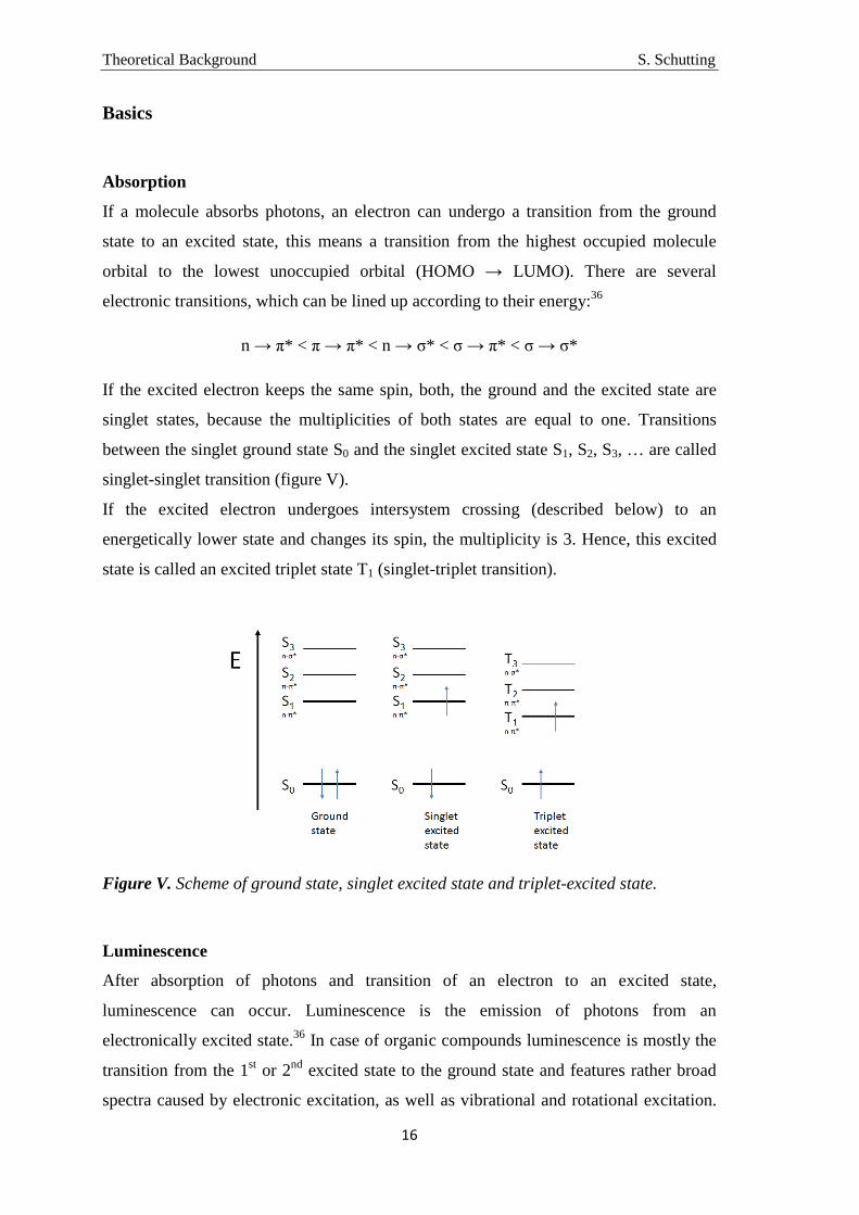
If the excited electron keeps the same spin, both, the ground and the excited state are
singlet states, because the multiplicities of both states are equal to one. Transitions
between the singlet ground state S0 and the singlet excited state S1, S2, S3, … are called
singlet-singlet transition (figure V).
If the excited electron undergoes intersystem crossing (described below) to an
energetically lower state and changes its spin, the multiplicity is 3. Hence, this excited
state is called an excited triplet state T1 (singlet-triplet transition).
Figure V. Scheme of ground state, singlet excited state and triplet-excited state.
Luminescence
After absorption of photons and transition of an electron to an excited state,
luminescence can occur. Luminescence is the emission of photons from an
electronically excited state.36 In case of organic compounds luminescence is mostly the
transition from the 1st or 2nd excited state to the ground state and features rather broad
spectra caused by electronic excitation, as well as vibrational and rotational excitation.
Theoretical Background S. Schutting
17
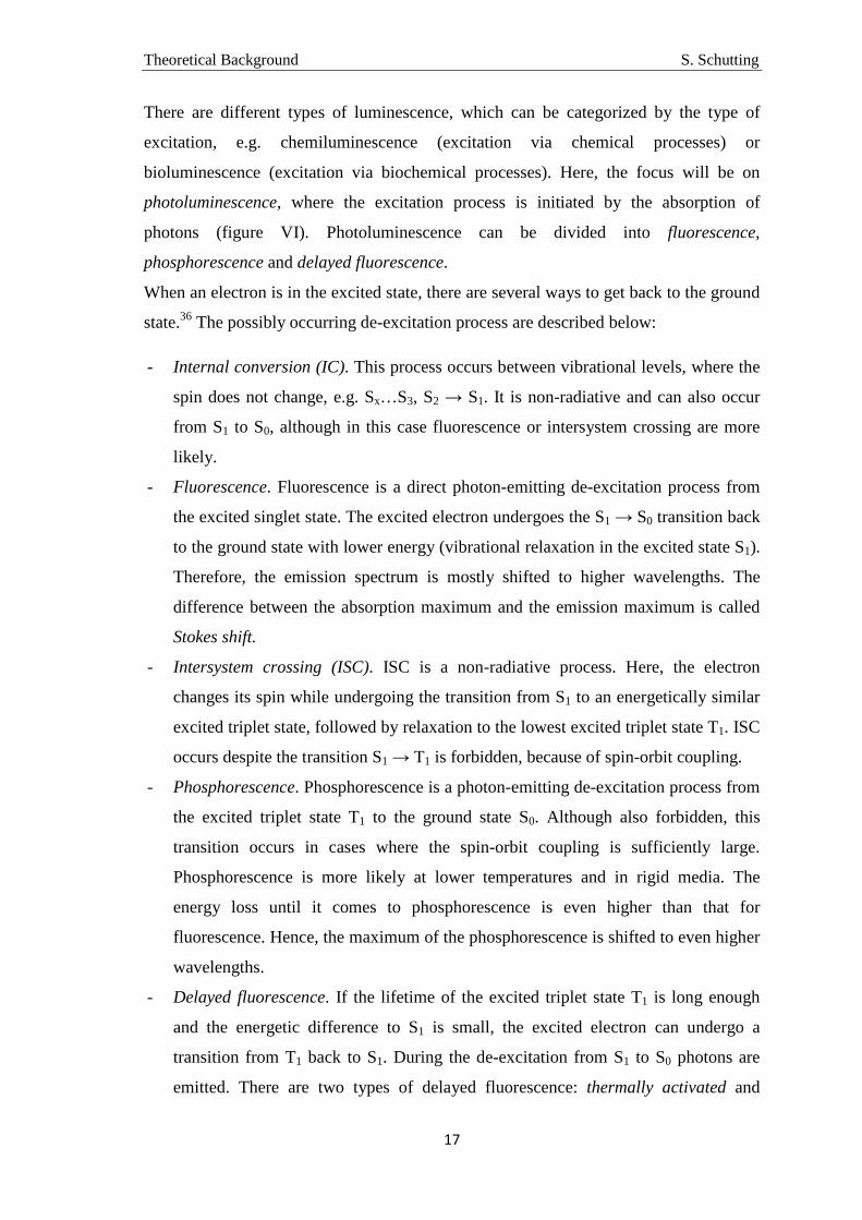
There are different types of luminescence, which can be categorized by the type of
excitation, e.g. chemiluminescence (excitation via chemical processes) or
bioluminescence (excitation via biochemical processes). Here, the focus will be on
photoluminescence, where the excitation process is initiated by the absorption of
photons (figure VI). Photoluminescence can be divided into fluorescence,
phosphorescence and delayed fluorescence.
When an electron is in the excited state, there are several ways to get back to the ground
state.36 The possibly occurring de-excitation process are described below:
- Internal conversion (IC). This process occurs between vibrational levels, where the
spin does not change, e.g. Sx…S3, S2 → S1. It is non-radiative and can also occur
from S1 to S0, although in this case fluorescence or intersystem crossing are more
likely.
- Fluorescence. Fluorescence is a direct photon-emitting de-excitation process from
the excited singlet state. The excited electron undergoes the S1 → S0 transition back
to the ground state with lower energy (vibrational relaxation in the excited state S1).
Therefore, the emission spectrum is mostly shifted to higher wavelengths. The
difference between the absorption maximum and the emission maximum is called
Stokes shift.
- Intersystem crossing (ISC). ISC is a non-radiative process. Here, the electron
changes its spin while undergoing the transition from S1 to an energetically similar
excited triplet state, followed by relaxation to the lowest excited triplet state T1. ISC
occurs despite the transition S1 → T1 is forbidden, because of spin-orbit coupling.
- Phosphorescence. Phosphorescence is a photon-emitting de-excitation process from
the excited triplet state T1 to the ground state S0. Although also forbidden, this
transition occurs in cases where the spin-orbit coupling is sufficiently large.
Phosphorescence is more likely at lower temperatures and in rigid media. The
energy loss until it comes to phosphorescence is even higher than that for
fluorescence. Hence, the maximum of the phosphorescence is shifted to even higher
wavelengths.
- Delayed fluorescence. If the lifetime of the excited triplet state T1 is long enough
and the energetic difference to S1 is small, the excited electron can undergo a
transition from T1 back to S1. During the de-excitation from S1 to S0 photons are
emitted. There are two types of delayed fluorescence: thermally activated and

Theoretical Background S. Schutting
18
triplet-triplet annihilation (TTA) initiated. Thermally activated means the
occurrence of the process is enhanced at higher temperatures. This process is also
called E-type delayed fluorescence (first observed with eosin).36 TTA means a
collision between two molecules in the excited triplet state (occurs in highly
concentrated samples). One of the molecules is then directly and non-radiative de-
excited to the ground state S0, whereas the other molecule undergoes a transition
back to the excited singlet state S1. This process is also called P-type delayed
fluorescence (first observed with pyrene).36 Spectrally delayed fluorescence
displays the same characteristics as “normal fluorescence”.
Figure VI . Perrin-Jablonski diagram.
Besides these de-excitation possibilities, there are several competitive ways of de-
excitation:36 intramolecular charge transfer, conformational change, electron transfer,
proton transfer, energy transfer, excimer formation, exciplex formation or
photochemical transformation.
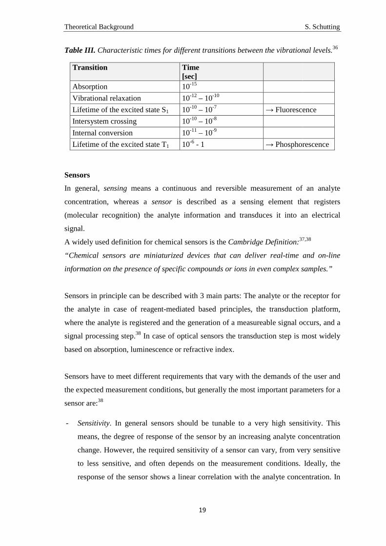
Table III shows the characteristic times for the transitions between the vibrational
levels. One should notice that absorption is the fastest, followed by vibrational
relaxation. In general, photon absorption is as fast as photon emission. In case of
fluorescence the enhanced time is caused by a short remain in the excited state. More
processes, like intersystem crossing and again short remains in the excited states, lead to
even longer times in case of phosphorescence and delayed fluorescence, although
delayed fluorescence shows the same spectral characteristics as fluorescence.
Theoretical Background S. Schutting
19
Table III. Characteristic times for different transitions between the vibrational levels.36
Transition Time [sec]
Absorption 10-15
Vibrational relaxation 10-12 – 10-10
Lifetime of the excited state S1 10-10 – 10-7 → Fluorescence
Intersystem crossing 10-10 – 10-8
Internal conversion 10-11 – 10-9
Lifetime of the excited state T1 10-6 - 1 → Phosphorescence
Sensors
In general, sensing means a continuous and reversible measurement of an analyte
concentration, whereas a sensor is described as a sensing element that registers
(molecular recognition) the analyte information and transduces it into an electrical
signal.
A widely used definition for chemical sensors is the Cambridge Definition:37,38
“Chemical sensors are miniaturized devices that can deliver real-time and on-line
information on the presence of specific compounds or ions in even complex samples.”
Sensors in principle can be described with 3 main parts: The analyte or the receptor for
the analyte in case of reagent-mediated based principles, the transduction platform,
where the analyte is registered and the generation of a measureable signal occurs, and a
signal processing step.38 In case of optical sensors the transduction step is most widely
based on absorption, luminescence or refractive index.
Sensors have to meet different requirements that vary with the demands of the user and
the expected measurement conditions, but generally the most important parameters for a
sensor are:38
- Sensitivity. In general sensors should be tunable to a very high sensitivity. This
means, the degree of response of the sensor by an increasing analyte concentration
change. However, the required sensitivity of a sensor can vary, from very sensitive
to less sensitive, and often depends on the measurement conditions. Ideally, the
response of the sensor shows a linear correlation with the analyte concentration. In

Theoretical Background S. Schutting
20
case of optical sensors the linear range is sometimes only a small section of the
allover dynamic range.
- Selectivity (Cross-sensitivity). The sensor should selectively and accurate respond to
the analyte that is in demand and should not be interfered by other species with
sometimes analyte-similar properties.
- Stability. The long-term stability during measurements or during long-term storage
is a very important parameter in different fields, e.g. storage of glucose sensor
stripes for diabetes patients or long-term measurements of the ocean acidification.
- Robustness. Sensors are sometimes applied under harsh conditions, such as high
temperatures, high pressure or extreme mechanical stress, and should ideally
withstand them.
Besides these parameters, a sensor system should be easy to miniaturize and free of
drifts, this means an appropriate protection against interferences should be applied, too.
A sensor should feature fast response and recovery times and easy-to-use-facilities.
Ideally, materials, production, maintenance and use should be cheap.

Theoretical Background S. Schutting
21
Optical Chemical Sensors
In case of optical chemical sensors the transduction mechanism is based on optical
properties of the analyte itself or an analyte-sensitive intermediate (here called
indicators or indicator dyes). Although there are challenges to meet, optical chemical
sensors show several advantages in comparison to routine techniques (e.g.
electrochemical sensors).
Challenges:
- In general, the indicator dyes (in case of reagent-mediated sensors) should feature
good photostability (bleaching prevention), high molar absorption coefficients and
quantum yields (high brightness), the possibility to tune their sensitivity and they
should be compatible with commercially available (low-cost) light sources, e.g.
LEDs. Ideally, they feature self-referencing spectral properties and the structural
conditions for a covalent coupling to the matrix.
- Matrix materials should show a low pH-dependent swelling and the possibility of
covalent coupling of the indicator to prevent leaching. The water uptake should be
high for pH sensors, but low for CO2 sensors. In case of multi-layer systems the
adhesion between the single layers and the support (fiber or planar support) should
be robust against mechanical and chemical stress.
- Optical pH sensors show dependency on the ionic strength and a narrow dynamic
rang (pKa ±1.5 pH unit).39
Advantages:
- In general, optical chemical sensors are easy to miniaturize and inexpensive.
- Via fiber optics measurements can be carried out in certain distances to the sample
site.
- The read-out can be carried out in a non-contact mode via an optical window, e.g.
in food packaging applications.
- There is no need for a separated reference element (as e.g. in precision
electrochemical sensors). Analyte-insensitive reference materials can be combined
with the analyte-sensitive chemistry in one sensing layer or one makes use of self-
referencing indicators. Self-referencing indicators are more robust and counteract
signal changes caused by leaching, photodegradation or aggregation.

Theoretical Background S. Schutting
22
- Optical sensors do not suffer from interferences of magnetic fields.
- Plastic type CO2 sensors are less affected by the ionic strength, than e.g. the
Severinghaus electrode.
- Optical sensors are easily tunable concerning their dynamic range and sensitivity. In
case of optical carbon dioxide sensors, the sensitivity of the sensors can be tuned
via the indicator (pKa value), the matrix and the base.
Optical chemical sensors can be influenced by various parameters, such as the sample
composition, temperature, sample polarity, viscosity or electrochemical properties. On
one hand, this enables optical sensors to measure these parameters, but on the other
hand, measurements are also influenced by them. Hence, experiments/measurements
should be carried out thoughtfully with respect to possible cross-talks.
Sensor Geometries
Optical chemical sensors can be manufactured in different geometries. The most
popular category is the fiber optic chemical sensor (FOCS) platform,38 using optical
fibers to guide the optical signal back and forward to the sample. FOCS can be divided
into active and passive formats. Active describes a direct modification of the fiber itself,
whereas for passive formats the fiber is only used for the transport of the optical signal.
Passive FOCS are often combined with a planar optode system at the end of the fiber.
Planar waveguide chemical sensor (PWCS) platforms represent the second biggest
category. Here, the actual sensing element is placed on a support (glass or plastic),
which can act as wave guiding element or only as support.
Both types, FOCS and PWCS are using mostly the transduction mechanisms of
absorption and luminescence. Colorimetric measurements (absorption) show lower
sensitivity, but are highly robust. Especially when the color change is preferred to be
also visible with the naked eye, absorption based sensors are widely used. Fluorescence
measurements are highly sensitive, cheap, easy to miniaturize and easy to carry out e.g.
excitation and emission light can be guided through the same fiber and can be separated
via an optical filter system. Besides, also the utilization of reflection or refractometric
principles is common.

Theoretical Background S. Schutting
23
Measurement Principles
One can distinguish between direct and reagent-mediated sensing.38 Direct sensing uses
the intrinsic optical properties of the analyte itself, such as absorption or luminescence.
In case of reagent-mediated sensors the optical properties of an analyte-sensitive
intermediate agent are utilized (indicator dye or indicator), especially when the analyte
does not show any useful optical properties. One third category, that should be noted,
are ionophore-based sensors. These sensors are not only based on an analyte-sensitive
intermediate. The analyte is registered by a receptor (ionophore), which does not show
any photophysical changes itself, but initiates another secondary process with respective
spectral changes.40,41
However, there are several sensing principles that can be made use of, especially for
reagent-mediated sensing. This thesis focuses on absorptive and fluorescence based
principles using pH-sensitive indicator dyes.
The following list shows an overview of the most popular principles:
- Absorption. Here, an analyte-dependent change (increase, decrease or ratiometric)
of the absorption maximum (UV-Vis range or near infrared) is observed.
Colorimetric measurements are generally very robust, but less sensitive than
fluorescence based principles. Absorption based optical sensors are used especially
when the color change should be visible with the naked eye.
- Luminescence. Luminescence in general represents a versatile and promising tool
for detection (directly or reagent-mediated). Not only its intensity can be used, but
also the spectral properties, its polarization or its temporal behavior. Thus,
luminescence enables a wide field of applications, e.g. monitoring at high sample
throughput or imaging.
In case of fluorescence, the analyte-dependent changes of different parameters, e.g.
decay time, energy transfer, quenching efficiency, intensity, polarization can be
used. Fluorescence based methods feature high sensitivity and are relatively easy to
realize.
Phosphorescent emitters are often used as references or as secondary emitters for
colorimetric indicators (Inner-filter effect).42
- Refractive index (Reflection). For measuring the refractive index (RI), the optical
fiber is partially decladded, light is sent through and detected on the opposite fiber
end. Thus, the refractive index of the investigated sample is measured.43,44 A special
Theoretical Background S. Schutting
24
case of these kind of sensors is the surface plasmon resonance (SPR) technique.
SPR is also based on the measurements of the refractive index of a thin layer of the
sample of interest, which is adsorbed on a metal layer.45 Via the thickness and
composition of the metal layer the sensitivity of the sensor can be tuned.46,47
- Reflectometry (Backscattering). This technique is based on the reflected
(backscattered) light response of the investigated sample after an initial light
impulse. It is also called optical time domain reflectometry.48
Materials
Optical chemical sensors can be tuned and enhanced for the requirements of the
measurement via “twisting screws” like the matrix or the indicator. In general, the
adhesion of the sensing chemistry to the wave guiding elements (fiber or planar support)
should be good and the support materials should not absorb light or show background
fluorescence.
Demands like high photostability, chemical stability, high molar absorption coefficients,
high quantum yields, compatibility with low-cost excitation sources and a tunable
sensitivity occur in case of the indicator dyes, which are the core components of
reagent-mediated optical sensors. Indicators with absorption/ luminescence intensity
maxima in the near infrared (NIR) region are highly desirable for several reasons, e.g.
dramatically reduced autofluorescence, low light scattering and the availability of low-
cost excitation sources and photodetectors.
Quantitatively, the matrix is the main component of an optical sensor. The indicator dye
(and possible other additives) is immobilized in the matrix. The easiest way of
immobilization is to simply embed the indicator. However, to prevent e.g. leaching, it is
preferred to immobilize the indicator dye via covalent coupling. Thus, leaching is
prevented, signal stability is enhanced, signal drifts diminished and long-term
applications are promoted. Hence, matrix materials should feature the structural
possibility for covalent coupling, as well as the indicators. Additionally, matrices should
be mechanically and chemically stable and they should take up adequate water (high
uptake for pH sensors; low uptake for CO2 sensors), but should display a low pH-
dependency of the swelling (in case of pH sensors) and the required permeability or
analyte-dissolving properties.
Theoretical Background S. Schutting
25
In this thesis optical carbon dioxide sensors based on pH-sensitive indicator dyes are
used. In the following sections state-of-the-art materials for optical pCO2 sensors will be
described. Additionally, caused by the relation to optical pH-sensors, materials for these
sensors will be briefly described, too.
Matrices
pH-sensors. For an optical pH sensor the matrix should be able to take up water and
therefore should be proton-permeable. Hence, the major part of optical pH sensors uses
hydrophilic matrix materials,39 such as cellulose and its acetates, polyurethane
hydrogels or polyacrylamides, but there are also less hydrophilic or even hydrophobic
alternatives, like sol-gels (less hydrophilic) or poly(vinyl chloride) (hydrophobic). The
latter category requires proton carriers, such as tetraphenylborate or similar.39
Carbon dioxide sensors. In earlier days, so called wet sensors based on buffer systems
were used, separated from the sample via a gas-permeable and ion-impermeable
membrane. When the water vapor pressure or the osmotic pressure of the sample was
extremely different to the sensor system, hydration/dehydration occurred and
recalibration was necessary.49 Additionally these systems suffered from intensity loss at
high pCO2 values and very slow response times at low pCO2 levels.
To overcome the drawbacks of the wet sensors, so called dry sensors, where plastic type
sensors developed by Mills et al.50,51 are the most common ones, were developed. Here,
the indicator dye is embedded in the polymer matrix together with a base (lipophilic
buffer), mainly a quaternary ammonium hydroxide. For optical carbon dioxide sensors
the water uptake of the matrix should be low. Hence, the polymer matrix should be
rather hydrophobic, permeable for carbon dioxide and impermeable for charged species
like protons, to prevent interferences by the pH of the (aqueous) sample. If the sensor
matrix itself can not fully meet these demands, a protection layer, e.g. silicone, is
necessary and acts as proton barrier. State-of-the-art polymer for optical carbon dioxide
sensors is ethyl cellulose with varying ethoxyl contents, although it shows a quite strong
temperature dependency and sensors show rather moderate long-term stability. Hence,
alternatives like amorphous perfluorinated polymers (PTFE derivatives) are under
investigation.

Theoretical Background S. Schutting
26
Indicators
Indicator dyes show ideally different spectral or photophysical properties with changing
analyte concentration. For both, optical pH and carbon dioxide sensors, the pKa value of
the indicator dye can give information about the dynamic range of the sensor. In case of
pH sensors, the optical sensors show the highest sensitivity in the equivalence point of
the titration/ calibration curve (pH = pKa; see also Henderson-Hasselbalch equation).
Hence, the rule of thumb means the dynamic range is ~pKa ± 1.5 pH unit, with respect
to the fact that the pKa value can be influenced by the environment, e.g. by the matrix.
For carbon dioxide sensors the rule of thumb says the higher the pKa value of the
indicator, the higher the sensitivity. The higher the pKa values the less carbon dioxide is
necessary to protonate the indicator, although this rule is rather applicable if one
compares indicators with similar structures.
Generally, one can classify pH-sensitive indicators as PPT (photoinduced proton
transfer) indicators, PET (photoinduced electron transfer) indicators or no PPT/ no PET
indicators.
- Indicators that show PPT (figure VII), e.g. 1-hydroxypyrene-3,6,8-trisulfonate
(HPTS; proton donor; pKa*< pKa ), have a different electron density in the excited
state than in the ground state. Therefore, they show different pKa values in the
excited state than in the ground state (lower pKa for proton donor molecules; higher
pKa for proton acceptors). This leads to a rather fast deprotonation (donors) or
protonation (acceptors) of the molecule. According to this acid-base behavior, both,
the absorption and luminescence spectra feature pH-dependency.
Figure VII . Scheme of photoinduced proton transfer (PPT)36 of an acidic dye (donor molecule; pKa*< pK a). Ka and Ka*: protolysis equilibrium values in the ground/excited state.

Theoretical Background S. Schutting
27
- PET indicators are chromophores (fluorophores) that become pH-sensitive by
attaching phenols or amines to their structure, also called PET-groups.52–55 These
PET-groups are acting as electron donors and hence, reduce the excited fluorophore
(photoinduced reduction). Hence, fluorescence is enhanced with increasing
protonation of the PET-group (figure VIII).
Figure VIII . Scheme of photoinduced electron transfer (PET).
- Indicators that show no PPT or PET feature still changes in absorption and
luminescence spectra related to a pH change. Although, this is not based on an acid-
base behavior, but on several processes, e.g. protolysis and lactonization equilibria
in case of fluorescein and its derivatives.
Common colorimetric pH-sensitive indicators for the UV-Vis range are
triphenylmethane dyes like thymol-blue56,57 or m-cresol-purple57,58 or phenol-red.59–61
Widely used fluorescent pH-sensitive indicators for the UV-Vis range are fluorescein
and its derivatives,62 coumarin and its derivatives63 or 1-hydroxypyrene-3,6,8-
trisulfonate (HPTS; excitable in the blue range of the spectrum) and its
derivatives.50,57,64–67
Common pH-sensitive indicators for the near infrared (NIR) region would be SNARF
(seminaphthorhodafluors) dyes,68 cyanine dyes69,70 or aza-BODIPY indicators.71
Carbon dioxide sensors. For optical carbon dioxide sensors based on the acid-base
chemistry of pH-sensitive indicator dyes (described above) state-of-the-art indicators
are thymol-blue, m-cresol-purple and especially HPTS (table IV) for fluorescence based
sensors.

Theoretical Background S. Schutting
28
Thymol-blue and m-cresol-purple are displaying two protonation steps, that means two
pKa values, where the first one is too low to show up in optical carbon dioxide sensors.
Here, only the pKa2 values are relevant for the dynamics of the optical sensors. Both
dyes show a rather low photostability and are only colorimetric indicators. To enable
luminescence read-out systems based on these dyes, one could make use of the so called
inner-filter effect, where the light of one or more secondary emitters is filtered
according to the pH-dependent colorimetric change of the indicator (figure IX).
Figure IX . Scheme of the inner-filter-effect. Left: layer system of the sensor. Right: Spectral theory.
HPTS was for a long time the indicator of choice for optical carbon dioxide sensors,
because of an ideal pKa value, high stability and a large stokes shift (~60 nm for the
ionic form in solution; see table IV).49 However, HPTS suffers from maxima at rather
short wavelengths for both forms, where only the ionic form is excitable in the blue part
of the spectrum. Addition of reference materials is often necessary to achieve reliable
measurements, but photobleaching (indicator, reference dye or both) can cause a
dramatic ratio change in this scheme.
Hence, alternative self-referencing (dual-emitting) indicators which overcome these
drawbacks, preferably in the NIR region, are highly desired.
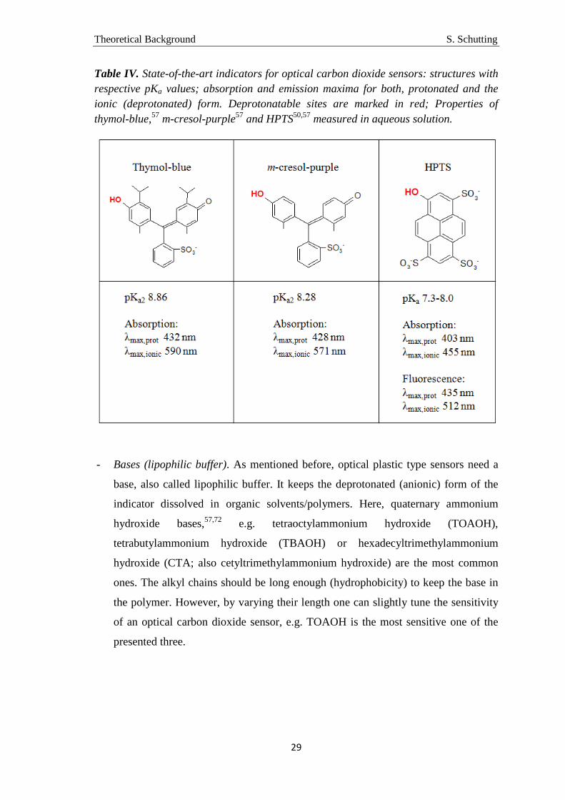
Theoretical Background S. Schutting
29
Table IV. State-of-the-art indicators for optical carbon dioxide sensors: structures with respective pKa values; absorption and emission maxima for both, protonated and the ionic (deprotonated) form. Deprotonatable sites are marked in red; Properties of thymol-blue,57 m-cresol-purple57 and HPTS50,57 measured in aqueous solution.
- Bases (lipophilic buffer). As mentioned before, optical plastic type sensors need a
base, also called lipophilic buffer. It keeps the deprotonated (anionic) form of the
indicator dissolved in organic solvents/polymers. Here, quaternary ammonium
hydroxide bases,57,72 e.g. tetraoctylammonium hydroxide (TOAOH),
tetrabutylammonium hydroxide (TBAOH) or hexadecyltrimethylammonium
hydroxide (CTA; also cetyltrimethylammonium hydroxide) are the most common
ones. The alkyl chains should be long enough (hydrophobicity) to keep the base in
the polymer. However, by varying their length one can slightly tune the sensitivity
of an optical carbon dioxide sensor, e.g. TOAOH is the most sensitive one of the
presented three.
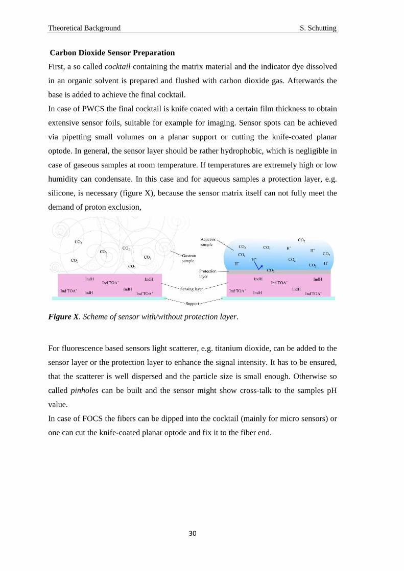
Theoretical Background S. Schutting
30
Carbon Dioxide Sensor Preparation
First, a so called cocktail containing the matrix material and the indicator dye dissolved
in an organic solvent is prepared and flushed with carbon dioxide gas. Afterwards the
base is added to achieve the final cocktail.
In case of PWCS the final cocktail is knife coated with a certain film thickness to obtain
extensive sensor foils, suitable for example for imaging. Sensor spots can be achieved
via pipetting small volumes on a planar support or cutting the knife-coated planar
optode. In general, the sensor layer should be rather hydrophobic, which is negligible in
case of gaseous samples at room temperature. If temperatures are extremely high or low
humidity can condensate. In this case and for aqueous samples a protection layer, e.g.
silicone, is necessary (figure X), because the sensor matrix itself can not fully meet the
demand of proton exclusion,
Figure X. Scheme of sensor with/without protection layer.
For fluorescence based sensors light scatterer, e.g. titanium dioxide, can be added to the
sensor layer or the protection layer to enhance the signal intensity. It has to be ensured,
that the scatterer is well dispersed and the particle size is small enough. Otherwise so
called pinholes can be built and the sensor might show cross-talk to the samples pH
value.
In case of FOCS the fibers can be dipped into the cocktail (mainly for micro sensors) or
one can cut the knife-coated planar optode and fix it to the fiber end.

Theoretical Background S. Schutting
31
Fields of Application - Optical Carbon Dioxide Sensors
Optical carbon dioxide sensors represent a promising tool for a variety of applications,
such as:
- Biotechnology (bioprocess monitoring)
- Medicine (capnography; blood gas analysis)
- Environmental science (monitoring of atmospheric carbon dioxide levels and
environmental processes)
- Meterological science
- Marine science (observation and investigation of ocean acidification and its effects
on the marine ecosystem)
- Chemical industry (process monitoring and controlling)
- Food and beverage science/industry (controlled atmosphere packaging; gas
diffusion into packages)
Fields like capnography or food packaging are dealing with rather high pCO2 values
and require less sensitive sensors, e.g. the pCO2 value of the exhaled air of the human
body contains around 3 to 6 kPa. Modern food packaging methods, also called MAP
(modified atmosphere packaging),73–75 use defined gas atmospheres, where oxygen is
excluded. The artificial atmosphere can be pure carbon dioxide, e.g. for bakeries,75 or a
mixture of nitrogen and carbon dioxide. In the case of vegetables and fruits the pCO2
value should be kept around ~5 kPa.73
In marine science the sensors have to meet different requirements. The atmospheric
level of pCO2 (0.04 kPa ≈ 400 µatm in the gas phase ≈ 11.6 µmol/l in seawater at
298.15 K), which is in equilibrium with the upper layer of the ocean requires very
sensitive sensors. On the other hand, there are volcanically active sites, e.g. the Aeolian
Islands (Sicily, Italy) in the Tyrrhenian Sea, where carbon dioxide is outgasing from the
seafloor, either continuous (bubbling) or discontinuous (CO2 enriched pore water
affected by tides). Around these seeps the pCO2 value in the seawater can reach
increased levels (up to several thousand µatm).

Theoretical Background S. Schutting
32
Comparison: Carbon Dioxide Detection Methods for Marine Applications
Introduction
So far only optical chemical sensors from the so called plastic type were discussed, as
the focus of this thesis was on these sensors. This section will give an overview on
routine techniques for measuring carbon dioxide in marine environments based on a
technical report written by S. Schutting and D. de Beer (2013; deliverable number D3.2
of the EU-project ECO2 (project number 265847); Technical report on chemical sensor
performance; DOI 10.3289/ECO2_D3.2.).
Technical data sheets were obtained from the homepages of CONTROS GmbH
(www.contros.eu) and Microelectrodes Inc. (www.microelectrodes.com). Additionally,
written requests via email were sent to CONTROS GmbH to Melanie Herrmann. Data
and information about the GasPro – dissolved CO2 probes were received from S.
Graziani (Sapienza University of Rome – CERI).
After a brief description of the most widely used sensing techniques for carbon dioxide,
commercially available sensing techniques will be compared in detail with alternative
prototype devices – the GasPro – dissolved CO2 probes and the multi-branched optical
carbon dioxide sensor system (MuFO; see also chapter 4) – concerning operational
parameters of the sensors and sensing systems.
The technical information will be complemented with experiences from users. In 2012
the HydroC device from CONTROS, the MuFO, the GasPro – dissolved CO2 probe and
a profiler with different electrodes were tested on a field trip at Panarea Island (Sicily,
Italy). Here, the feedback of the diving team is summarized. In 2013 the MuFO device
was used for a lab experiment at SAMS (Scottish Association for Marine Science)
Institute in Oban (Scotland) and the feedback of the users is also summarized.
Carbon dioxide can be measured optically or electrochemically. The most relevant
detection method based on electrochemistry is the Severinghaus electrode. Optical
techniques are infrared spectroscopy, spectrophotometry or optical chemical sensors.
Severinghaus electrode. The Severinghaus electrode was developed in the late 1950´s
and was long time the method of choice for measuring pCO2 in solutions, especially in
blood.76–78 It consists of a pH glass electrode, which is placed in a buffer chamber
Theoretical Background S. Schutting
33
(mostly sodium bicarbonate solution). The buffer is separated from the sample via a
hydrophobic gas-permeable and ion-impermeable membrane, where CO2 can enter the
chamber, but ions can not. CO2 then reacts with the buffer solution in the following
way:
CO2 + H2O ↔ H2CO3 ↔ HCO3- + H+
The protons change the pH value within the buffer chamber. Thus, the CO2 caused pH
change is measured by the pH electrode.
The Severinghaus electrode shows excellent selectivity.79 However, compared to optical
chemical sensors based on the same reaction principle, the electrode suffers from
electromagnetic interferences and has a slower response.
Infrared (IR) spectroscopy. IR spectroscopy is a direct measurement method. An
infrared spectrum is like a fingerprint of a molecule, as in case of carbon dioxide.
Organic molecules absorb infrared radiation and convert it into energy of molecular
vibration. Carbon dioxide shows characteristic vibrations at 2349 cm-1 (asymmetrical
stretch) and at 546 cm-1 (bending vibration), which are observable in the IR spectrum,
because of a dipole change.80 The symmetrical stretch at 1735 cm-1 is inactive in the IR,
because it does not change the dipole of the molecule.
IR spectroscopy is used in several fields as detection method of choice,81 for example
medicine (capnography),82,83 investigation of the carbon cycle (soil respiration)84 and
others. It is a fast61 and non destructive method, but is mostly suitable for measurements
in gaseous phase85,86 since water causes a significant interference. The instruments are
usually rather bulky and expensive.
Sepctrophotometry. This detection technique is an indirect measurement making use of
the pH affecting property of carbon dioxide by applying spectrophotometry within an
equilibrated pH-sensitive dye solution of known characteristics.87,88
The compared optical carbon dioxide sensors are based on the following principle:
CO2 + H2O + Ind-TOA+ ↔ TOA+HCO3- + IndH
In these so called plastic type sensors50,51,57,89 the indicator dye (Ind-; IndH) is
embedded in the polymer matrix together with a base (TOA+; lipophilic buffer). When
CO2 and water form bicarbonate ions and protons, the protons are changing the

Theoretical Background S. Schutting
34
protonation state of the indicator dye. The indicator ideally features different spectral
properties for both, the protonated and ionic (deprotonated) form, which can be used for
analysis. Materials (matrices, indicators and bases), measurement principles, as well as
sensor geometries have been already discussed in previous chapters of this thesis. These
optical carbon dioxide sensors feature low affection by ionic strength, are easy to
miniaturize and are therefore, a promising alternative to the presented up-to-now-
routine techniques.
Besides these techniques, carbon dioxide can also be analyzed via Gas chromatography
(GC). Gas chromatography is a very popular detection method for carbon dioxide and
other greenhouse gases.90 State-of-the-art equipment would be e.g. PORAPLOT Q or
PORAPLOT Q UltiMetal from Agilent Technologies (www.agilent.com) and a thermal
conductivity detector (TCD) or a barrier ionization discharge (BID) detector.
It shows high sensitivity and high sample trough-put,90 but in case of non-gaseous
samples, for example seawater, a respective sample preparation or accurate sampling is
necessary. Therefore, a direct on-line measurement, e.g. in marine science, is hardly
realizable and the sample preparation is mostly cost- and time consuming.
Technical Comparison
Here, a comparison concerning operational parameters of the carbon dioxide sensors
and sensing systems listed below will be shown and summarized in table V in the end of
this section. Companies and developing scientists often provide the measuring range of
their devices in ppm without specifying which ppm is meant: either mg CO2/l or volume
percent* 10000 at 1 atm. In the following section the units given from the manufacturer
will be listed, as well as a respective concentration in µmol/l or similar. The carbon
dioxide concentration can be calculated from partial pressure, temperature and salinity.
Hence, the accuracy of the CO2 measurements is not only dependent on the sensors
behavior, but also on the accuracy of these parameters. Compared systems will be:
- HydroC from CONTROS GmbH
- GasPro (dissolved CO2 probes) from Sapienza University of Rome
- Optical chemical sensors (MuFO) from Graz University of Technology
- Severinghaus CO2 sensors (microelectrode MI 720) from Microelectrodes Inc.
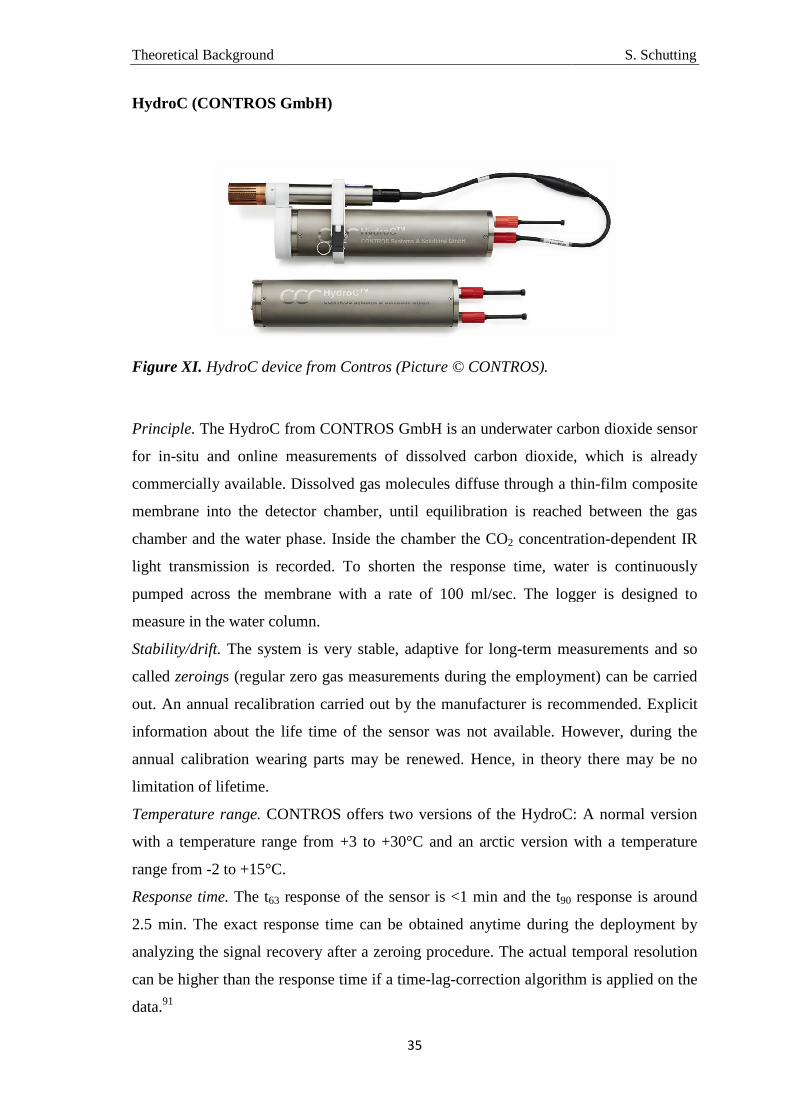
Theoretical Background
HydroC (CONTROS GmbH)
Figure XI. HydroC device from Contros (Picture ©
Principle. The HydroC from CONTROS GmbH
for in-situ and online measurements of dissolved
commercially available. Dissolved gas molecules diffuse through a thin
membrane into the detector chamber, until equilibration is reached between
chamber and the water phase. In
light transmission is recorded. To shorten the response time, water is continuously
pumped across the membrane with a rate of 100 ml/
measure in the water column.
Stability/drift. The system is very stable,
called zeroings (regular zero gas measurements during the employment) can be carried
out. An annual recalibration
information about the life time of the sensor was not available. However,
annual calibration wearing parts may be renewed. Hence, in theory there may be no
limitation of lifetime.
Temperature range. CONTROS offers
with a temperature range from +3 to +30°C and an arctic version with a temperature
range from -2 to +15°C.
Response time. The t63 response of the sensor is <1 min and the t
2.5 min. The exact response time can be obtained anytime during the deployment by
analyzing the signal recovery after a zeroing procedure. The
can be higher than the response time if a time
data.91
35
GmbH)
vice from Contros (Picture © CONTROS).
from CONTROS GmbH is an underwater carbon d
situ and online measurements of dissolved carbon dioxide
commercially available. Dissolved gas molecules diffuse through a thin
membrane into the detector chamber, until equilibration is reached between
phase. Inside the chamber the CO2 concentration
light transmission is recorded. To shorten the response time, water is continuously
pumped across the membrane with a rate of 100 ml/sec. The logger is designed to
measure in the water column.
The system is very stable, adaptive for long-term measurements and so
(regular zero gas measurements during the employment) can be carried
ration carried out by the manufacturer is recommended
information about the life time of the sensor was not available. However,
annual calibration wearing parts may be renewed. Hence, in theory there may be no
CONTROS offers two versions of the HydroC:
with a temperature range from +3 to +30°C and an arctic version with a temperature
response of the sensor is <1 min and the t90
ct response time can be obtained anytime during the deployment by
analyzing the signal recovery after a zeroing procedure. The actual temporal resolution
can be higher than the response time if a time-lag-correction algorithm is applied on the
S. Schutting
is an underwater carbon dioxide sensor
carbon dioxide, which is already
commercially available. Dissolved gas molecules diffuse through a thin-film composite
membrane into the detector chamber, until equilibration is reached between the gas
concentration-dependent IR
light transmission is recorded. To shorten the response time, water is continuously
. The logger is designed to
term measurements and so
(regular zero gas measurements during the employment) can be carried
is recommended. Explicit
information about the life time of the sensor was not available. However, during the
annual calibration wearing parts may be renewed. Hence, in theory there may be no
two versions of the HydroC: A normal version
with a temperature range from +3 to +30°C and an arctic version with a temperature
response is around
ct response time can be obtained anytime during the deployment by
actual temporal resolution
correction algorithm is applied on the

Theoretical Background S. Schutting
36
Measuring range. The standard measuring range is from 200 to 1000 ppm or, if
required, the calibration can be extended up to 6000 ppm. As calculation in mg/l would
result in an impossible range for dissolved CO2 (200-6000 mg CO2/l), it is assumed, that
this values correlate to 6.8*10-3 to 3.4*10-2 mmol/l and 2.0*10-1 mmol/l, respectively.
Maintenance. The HydroC device has a power consumption of 300 mA and additionally
600 mA for the water pump. The power consumption can be customized by using the
integrated sleep mode and a smaller (less consumable) water pump, as well as by
adapting the temperature control settings of the sensor. The device can be powered
either via cable, by non-rechargeable batteries or by rechargeable batteries. The latter
can be charged via cable while they are inside of the housing. The membrane should be
changed (by the user) every 3 months in case of continuous use or when strong fouling
occurs. An annual recalibration of the HydroC device is recommended.
Deployment. CONTROS offers the HydroC device as a “Plug and Play” system
including the software, a sensor manual and an USB adapter, as well as a connection
cable for configuration or lab purposes. The HydroC can be easily handled under water
by only one person. Besides stationary measurements on moorings, it can be used for
transect measurements by trawling, scuba divers, an AUV (autonomous underwater
vehicle) or a ROV (remotely operated underwater vehicle). Measurements in the
sediment are not possible. Due to different types and sizes of power sources, the
deployment time depends on the frequency of measurements and the power
consumption of the device. The turnover time can be only one hour, including data
download, data check and battery exchange.
Userfriendliness. The system shows high accuracy (1%), it has an internal datalogger
and can be connected to other devices, e.g. a CTD (conductivity, temperature and depth
measuring device). The software is understandable and easy to use. Data can be
processed fast. Additionally, CONTROS offers assistence for an optimal configuration
of the device to meet the requirements of the user.
Depth. The device can be used up to 6000 m water depth.
Size. ø 90 x 376 mm, 4.7 kg in air (2.2 kg in water)
Costs. The HydroC device is commercially available for around 24000 € (Generation II
with Sea-Bird pump SBE-5T, 2000 m depth rating, 200-1000 ppm, RS 232, +3 to
+30°C, SubConn connector, internal datalogger) including an accessories kit (software
detect 2.0 incl. manual, 3 spare membranes, USB 2.0 to RS 232 adapter, sensor manual

Theoretical Background
and certification), cable equipment and offshore case. 5 membranes are available for
500 €. An annual recalibration costs 1750 €.
GasPro - Dissolved CO
Figure XII. The GasPro
Principle. The GasPro device
for long-term monitoring applications and is
configurations are in use to meet the requireme
conditions and experimental demands. The device measure
the gas phase or in the soil.
pressure of the surrounding dissolved gas is measur
molecules diffuse through a TeflonAF membrane into the
chamber. The detector is a 20 mm ø CO
“GasPro-pCO2” for deployment in marine environments up to a depth of 50
presented. The device is designed for long
with low power consumption. Thus, pumps are usually not integrated in the system,
although they can be adapted for a faster response e.g. during short
Stability/drift. Although, there is usually no artificial hydrodynamics (no pumps) that
can enhance the prevention of biofilm growth, the membrane material is rather resistant
against biofouling. In case of highly eutrophic environments an occasi
the membrane is recommended to prevent drifts. No zeroing can be performed with this
37
and certification), cable equipment and offshore case. 5 membranes are available for
€. An annual recalibration costs 1750 €.
CO2 Probes (Sapienza University of Rome)
The GasPro - Dissolved CO2 probe.
GasPro device is a small, light-weight, accurate and
term monitoring applications and is in continuous development.
configurations are in use to meet the requirements of different environments, site
conditions and experimental demands. The device measures dissolved CO
the gas phase or in the soil. In case of measurements in the water phase the partial
pressure of the surrounding dissolved gas is measured. Here, the d
molecules diffuse through a TeflonAF membrane into the small
chamber. The detector is a 20 mm ø CO2-NDIR cell. In the following, the model
for deployment in marine environments up to a depth of 50
presented. The device is designed for long-term applications and therefore, developed
with low power consumption. Thus, pumps are usually not integrated in the system,
although they can be adapted for a faster response e.g. during short-term meas
Although, there is usually no artificial hydrodynamics (no pumps) that
can enhance the prevention of biofilm growth, the membrane material is rather resistant
In case of highly eutrophic environments an occasi
the membrane is recommended to prevent drifts. No zeroing can be performed with this
S. Schutting
and certification), cable equipment and offshore case. 5 membranes are available for
and low-cost prototype
in continuous development. Different
nts of different environments, site
dissolved CO2 in water, in
In case of measurements in the water phase the partial
ed. Here, the dissolved gas
small-volume detector
In the following, the model
for deployment in marine environments up to a depth of 50 to 60 m is
term applications and therefore, developed
with low power consumption. Thus, pumps are usually not integrated in the system,
term measurements.
Although, there is usually no artificial hydrodynamics (no pumps) that
can enhance the prevention of biofilm growth, the membrane material is rather resistant
In case of highly eutrophic environments an occasional cleaning of
the membrane is recommended to prevent drifts. No zeroing can be performed with this
Theoretical Background S. Schutting
38
system. The sensors and logger are highly robust. So far no failure was observed during
deployment. No data on the total life time of the system is available.
Temperature range. The probe operates at temperatures from 0 to 40°C.
Response time. The sensor shows a t90 response time of 40 sec. However, the unit
response time depends on gas diffusion rates across the membrane and equilibration
between the gas volume of the sensor chamber and the surrounding water. Without
pumps the systems response depends on currents and concentration gradients, with a
minimum of ~2 min being required.
Measuring range. The measuring range (zero resolution 1 ppm) is 0 to 5000 ppm (0 to
1.7*10-1 mmol/l) with a full scale resolution of 15 ppm (5.1*10-4 mmol/l). If required,
the device can be calibrated to higher ranges.
Maintenance. The device can be powered either by non-rechargeable batteries for long-
term applications (must be replaced after approx. 4000 measurements) or by
rechargeable batteries (chargeable via a cable). The loggers require 2 batteries. The
integrated data logger and low power consumption (6-12 VDC; warm-up 2-30 min/40
mA) of the sensor make it suitable for long-term monitoring with sample frequencies of
either 1/min, 1/10min, 1/hour, 1/day, 1/week or 1/month. The data format is ASCII with
real time clock information (date, hour, minute, second; resolution: 1 sec).
Deployment. Besides batteries no exchange of parts is needed between deployments. If
the batteries need to be exchanged, the turnover time is about 1 hour, including removal
of biofouling. The GasPro device can be used as stand-alone (SD-card as removable
memory) or connected to control units for data transmission in real time. Downloading
of 4000 data points takes approximately 10 minutes. The operation time depends on the
measurement interval. When measuring every 10 minutes, the batteries will have
sufficient power for at least 4 weeks. When the interval is longer, the deployment time
can be proportionally longer.
Userfriendliness. As it is a prototype the software is simple, the interface may be
improved and manuals are not available. The servicing, calibration and redeployment
can be done by only one person. Without a pump the battery life was very long and the
device could be shifted from location to location without need of battery change.
Depth. Under water it can be used at operation depths of 60 m (standard), 100 m or 200
m.
Size. ø 78 x 283 mm, 0.7 kg in air (slightly positively buoyant in seawater).

Theoretical Background
Costs. The material costs for the dissolved CO
of work not included). 2 batteries for loggers
housing materials and the machining for the different prototypes the costs can vary
widely.
Optical Chemical Sensors/
Figure XIII. Optical chemical sensors combined with the multicarbon dioxide sensor system (bundles of 20 fibers each.
Principle. This sensor system featu
collective excitation source and read
the habitat, within the range of the optode length. It can thus provide the CO
in many sites within that habitat, in
corals, etc. The measurement principle is based on optical chemosensing.
of the multi-branched optical carbon dioxide sensor system is described in more detail
in chapter 4 of this thesis
Stability/drift. The photostability of the used dye
poisoning of the sensor are
sensing foils on the fiber
39
The material costs for the dissolved CO2 probe up to now are appr. 2500
. 2 batteries for loggers cost 27 € each. Depending on both the
housing materials and the machining for the different prototypes the costs can vary
ensors/ MuFO (Graz University of Technology
Optical chemical sensors combined with the multicarbon dioxide sensor system (see also chapter 4). 100 optodes positioned o
s each.
This sensor system features 100 freely positionable
excitation source and read-out. The optodes can be positioned anywhere in
the habitat, within the range of the optode length. It can thus provide the CO
that habitat, including e.g. sediments, watercolumn, musselbeds,
corals, etc. The measurement principle is based on optical chemosensing.
branched optical carbon dioxide sensor system is described in more detail
of this thesis.
The photostability of the used dye and the protection ability against
poisoning of the sensor are the limiting factors during long-term measurements. The
ensing foils on the fiber tips should be exchanged periodically (time interval depends
S. Schutting
obe up to now are appr. 2500 € (hours
€ each. Depending on both the
housing materials and the machining for the different prototypes the costs can vary
versity of Technology)
Optical chemical sensors combined with the multi-branched optical 100 optodes positioned on a stick in
res 100 freely positionable CO2 optodes with
out. The optodes can be positioned anywhere in
the habitat, within the range of the optode length. It can thus provide the CO2 dynamics
sediments, watercolumn, musselbeds,
corals, etc. The measurement principle is based on optical chemosensing. The principle
branched optical carbon dioxide sensor system is described in more detail
and the protection ability against
term measurements. The
tips should be exchanged periodically (time interval depends
Theoretical Background S. Schutting
40
on the dye and the illumination intervals). Information about the life time is not yet
available as the development of the MuFO system is still ongoing.
Temperature range. So far the optical sensors of the prototype were tested in a
temperature range from +5 to +35°C. Their temperature-dependence is quite high.
Therefore it is necessary to either calibrate at the same temperature as the measurement
(if the measurement temperature is expected to be rather constant) or to develop a
mathematical description of the temperature-dependence. In the latter case the
temperature has to be monitored next to the sensors to include it later on in the data
analysis.
Response time. Generally, the optical CO2 sensors measure continuously. In case of
alternating pCO2 values in the laboratory the t90 response time was about 20 sec. At
lower pCO2 values the response times can be even longer.
Measuring range. The measuring range of the optodes can be adjusted to the
requirement of the user starting from ~200 ppm (6.8*10-3 mmol/l) up to a few thousand
ppm (e.g. 5000 ppm = 1.7*10-1 mmol/l) by choosing the suitable dye for the desired
concentration range.
Maintenance. The accumulators of the MuFO have to be charged via cable after appr.
24 h of permanent use (duration of charging: ~10 h). The accumulators of the camera
have to be recharged or exchanged every 9 h (duration of charging: ~2 h) and are the
limiting factor for the deployment length. Data are saved to the SD card of the camera.
For both, charging the camera batteries and downloading the data, the camera has to be
removed from the MuFO housing, after which the camera has to be refocused. Thus the
turnover time between deployments is approximately 10 hours.
Deployment. The MuFO prototype has an operating software and manuals for the sensor
preparation, the calibration, the general handling and the software. Connected to a
computer it can be controlled manually, e.g. for lab-applications, or programmed for an
auto-start for a later measurement, e.g. for the diving team. The sensor tips are flexible,
robust and well protected by metal sleeves. The contact surface is very small (ø ~1.5
mm). Thus, the optodes can be used for profiling too, either in a fixed array of sensors
or by using a single optode that penetrates the sediments step wise. Measurements in the
gas phase are possible, too.
Userfriendliness. After long-term measurements the amount of produced data is huge.
Therefore, the analysis can take quite a long time. The positioning of the sensors is
complicated.

Theoretical Background
Depth. Up to now the optical sensors were tested in water depths down to 20 m.
Size. ø 280 x 400 mm; fiber
Costs. Optodes are inexpensive (
Price-calculation depends strongly on the
material costs for the MuFO
Severinghaus CO2 Sensors
Figure XIV. The Severinghaus COMicroelectrodes Inc.)
Principle. The Severinghaus electrode is an electrochemical sensor for CO
measurements. It is a pH electrode in a chamber with buffer solution (usually a 1 mM
NaHCO3 solution with a pH of 8.2). Through a membrane the CO
chamber can equilibrate with the sample. The pH in the chamber shifts proportionally to
the samples CO2 level and this pH is measured.
Stability/drift. The sensors have a tendency to drift of appr
in the concentration range below 200 µM, the electrode shows a drift of about 1
per day). Therefore, they must be calibrated regularly. This limits their application for
long term monitoring, although they
sensing surface is small, the sensitivity to biofouling is very limited.
used for several weeks to months, after which the membrane should be exchanged. The
pH transducer has a life time of appr. 1 year. During measurements weak volatile acids
can cause interferences.
Temperature range. This information was not available.
Response time. According to the specifications, the pCO
time of less than 1 min. However, stabilization times of several minutes are more
typical. Therefore, measurements that are made frequen
41
now the optical sensors were tested in water depths down to 20 m.
fiber length 5-6 m
expensive (selfmade sensing foils cost up to a few
calculation depends strongly on the material costs of the read
material costs for the MuFO up to now are around 3000 € (hours of work not included
Sensors – Microelectrode MI 720 (Microelectrodes Inc.
The Severinghaus CO2 sensor microelectrode MI 720 (Pictur
The Severinghaus electrode is an electrochemical sensor for CO
measurements. It is a pH electrode in a chamber with buffer solution (usually a 1 mM
solution with a pH of 8.2). Through a membrane the CO2 concent
chamber can equilibrate with the sample. The pH in the chamber shifts proportionally to
and this pH is measured.
The sensors have a tendency to drift of appr. 1 mV/day (w
ion range below 200 µM, the electrode shows a drift of about 1
Therefore, they must be calibrated regularly. This limits their application for
long term monitoring, although they are well applicable to monitor dynamics. As the
e is small, the sensitivity to biofouling is very limited.
used for several weeks to months, after which the membrane should be exchanged. The
pH transducer has a life time of appr. 1 year. During measurements weak volatile acids
This information was not available.
According to the specifications, the pCO2 microelectrode has a response
time of less than 1 min. However, stabilization times of several minutes are more
fore, measurements that are made frequently are best binned over 3 min
S. Schutting
now the optical sensors were tested in water depths down to 20 m.
s cost up to a few € per sensor).
the read-out device. The
hours of work not included).
Microelectrodes Inc.)
sensor microelectrode MI 720 (Picture ©
The Severinghaus electrode is an electrochemical sensor for CO2
measurements. It is a pH electrode in a chamber with buffer solution (usually a 1 mM
concentration in this
chamber can equilibrate with the sample. The pH in the chamber shifts proportionally to
1 mV/day (when measuring
ion range below 200 µM, the electrode shows a drift of about 1-3 µM
Therefore, they must be calibrated regularly. This limits their application for
to monitor dynamics. As the
e is small, the sensitivity to biofouling is very limited. The sensors can be
used for several weeks to months, after which the membrane should be exchanged. The
pH transducer has a life time of appr. 1 year. During measurements weak volatile acids
microelectrode has a response
time of less than 1 min. However, stabilization times of several minutes are more
tly are best binned over 3 min.

Theoretical Background S. Schutting
42
Measuring range. The sensors behave log-linear from ca 3 µmol/l to 30 mmol/l, this
means from below air saturation to CO2 saturated water. The data sheet from the
company indicates a range of 0.1-100 mmol/l and 4.4-440 ppm, both may be a mistake.
Upon request, the company elucidated that the sensors are tested at 0.1 and 30% carbon
dioxide in a gas mixture.
Maintenance. The maintenance depends on the electronic loggers on which they are
mounted. The company provides an amplifier (MV-ADPT Millivolt Adapter) with a
battery life of 5 years. The loggers will need further battery power for data acquisition
and storage. This will depend on the brand of logger. When the amplifier MV-ADPT
Millivolt Adapter is used for the primary amplification, the battery charging or
exchange depends further entirely on the logger system in which it is embedded. Also
the downloading of the data depends on the logger system. The time needed for
maintenance of the sensor between deployments is approximately 30 minutes. The
chamber with membrane has to be regularly exchanged, which is a very simple
operation. After this exchange the sensor must be recalibrated.
Deployment. The servicing, calibration and redeployment can be done by only one
person. When mounted on basic loggers, deployment can be done by scuba diving or
snorkeling. The sensors can measure in the water column and inside sediments.
Userfriendliness. Electrodes are easy to handle. They are small and do not need
complicated software solutions.
Depth. The electrode can be pressure compensated and can be used in water depths
from at least 2000 m. High pressure will affect the sensor offset, thus an in situ
calibration is needed. For this a water sample from the deployment depth must be taken
and analyzed for pH, DIC and alkalinity. From the appropriate equilibrium values the
total carbonate system can be calculated, including the pCO2.15
Size. ø 6 x 86 mm
Costs. A pCO2 microelectrode from Microelectrodes Inc. is commercially available for
490 USD (≈ 366 €). Additionally, the costs for a logger house plus electronics need to
be included. The preamplifier costs 199 USD (≈ 149 €).
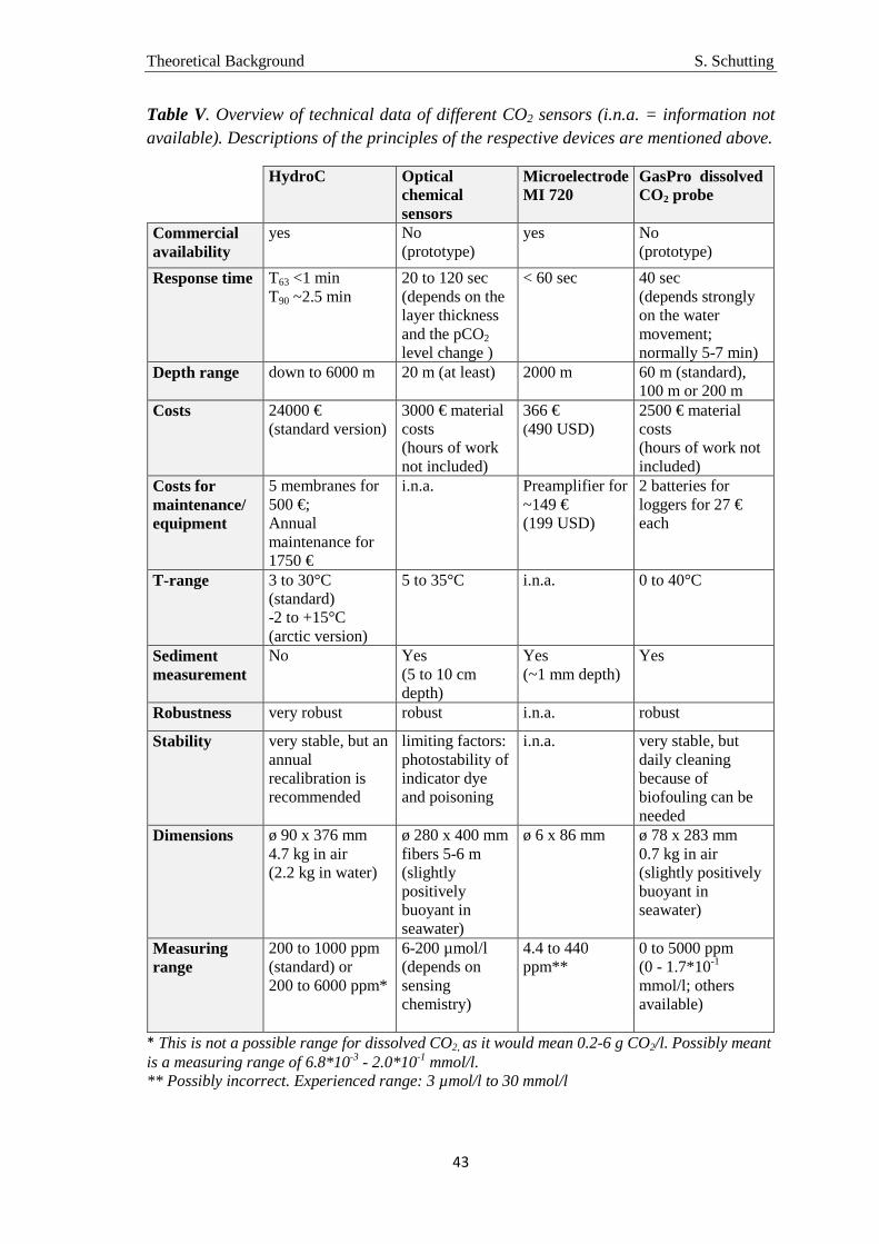
Theoretical Background S. Schutting
43
Table V. Overview of technical data of different CO2 sensors (i.n.a. = information not available). Descriptions of the principles of the respective devices are mentioned above.
HydroC Optical chemical sensors
Microelectrode MI 720
GasPro dissolved CO2 probe
Commercial availability
yes No (prototype)
yes No (prototype)
Response time T63 <1 min T90 ~2.5 min
20 to 120 sec (depends on the layer thickness and the pCO2 level change )
< 60 sec 40 sec (depends strongly on the water movement; normally 5-7 min)
Depth range down to 6000 m 20 m (at least) 2000 m 60 m (standard), 100 m or 200 m
Costs 24000 € (standard version)
3000 € material costs (hours of work not included)
366 € (490 USD)
2500 € material costs (hours of work not included)
Costs for maintenance/ equipment
5 membranes for 500 €; Annual maintenance for 1750 €
i.n.a. Preamplifier for ~149 € (199 USD)
2 batteries for loggers for 27 € each
T-range 3 to 30°C (standard) -2 to +15°C (arctic version)
5 to 35°C i.n.a. 0 to 40°C
Sediment measurement
No Yes (5 to 10 cm depth)
Yes (~1 mm depth)
Yes
Robustness very robust robust i.n.a. robust
Stability very stable, but an annual recalibration is recommended
limiting factors: photostability of indicator dye and poisoning
i.n.a. very stable, but daily cleaning because of biofouling can be needed
Dimensions ø 90 x 376 mm 4.7 kg in air (2.2 kg in water)
ø 280 x 400 mm fibers 5-6 m (slightly positively buoyant in seawater)
ø 6 x 86 mm
ø 78 x 283 mm 0.7 kg in air (slightly positively buoyant in seawater)
Measuring range
200 to 1000 ppm (standard) or 200 to 6000 ppm*
6-200 µmol/l (depends on sensing chemistry)
4.4 to 440 ppm**
0 to 5000 ppm (0 - 1.7*10-1 mmol/l; others available)
* This is not a possible range for dissolved CO2, as it would mean 0.2-6 g CO2/l. Possibly meant is a measuring range of 6.8*10-3 - 2.0*10-1 mmol/l. ** Possibly incorrect. Experienced range: 3 µmol/l to 30 mmol/l

Theoretical Background S. Schutting
44
Experiences from Users
In 2012 the compared devices CONTROS HydroC, Optodes (MuFO), the GasPro –
dissolved CO2 probe and a profiler equipped with different glass electrodes were tested
all together off Panarea Island (Sicily, Italy). In the submarine exhalative field located
east of Panarea Island, the devices were tested at different sites with different
geochemical characteristics. Sites with and without CO2 seeping were studied. The
diving teams operating with the devices were from the HYDRA Institute (Elba, Italy)
and GEOMAR/CONTROS (Kiel, Germany). The GasPro device was also used during a
field trip to CO2 seeps in a coral reef in New Guinea.
In 2013 the multi-branched optical carbon dioxide sensor system (MuFO) was applied
again off Panarea Island. Additionally, it was tested at the SAMS (Scottish Association
for Marine Science; Oban, Scotland) from Anna Lichtschlag and Peter Taylor in a lab
experiment.
The divers and scientists gave the following feedback:
HydroC. The HydroC device from CONTROS was small and very well manageable
under water for the divers. On one occasion the battery was incorrectly connected and
consequently the device did not log data. In the meantime measures have been taken to
avoid this problem. The very short response time enabled measurements of the
dynamics better than the GasPro device.
GasPro. A pump can be attached to the GasPro device, resulting in similar response
times than the HydroC. The GasPro was easy to handle, because of its small
dimensions. Because of its low weight it was slightly positively buoyant in seawater and
the divers had to attach additional weight on the device. Near seeps with strongly
reducing fluid chemistry biofouling occurred on the membrane, that had to be removed
every 3 days (it should be noted, that all sensors suffered from biofouling near these
seeps). Use of an external pump would have reduced biofouling of the membrane.
Biofouling is most easily removed with freshwater. On one occasion a logger had
stopped after 10 measurements. A file with settings appeared empty, probably because
of mishandling of the software. The file was replaced with one from another logger,
after which the problem was solved and did not reoccur.
Comparison HydroC and GasPro. The HydroC and the GasPro are compareable
devices. The HydroC is more expensive, but this version with pump has a shorter

Theoretical Background S. Schutting
45
response time, is supported by the services of the company, can be auto-zeroed to
compensate for drift and can be used at much larger depths. The tested version of the
GasPro device was a low-cost solution with basic (and reliable) performance. Therefore,
it can be used in larger numbers, e.g. to monitor carbon dioxide dynamics in a
heterogeneous habitat surrounding a seep. Also the GasPro can be equipped with a
pump to reduce response times. Obviously, the use of pumps will compromise the
battery life and thereby user-friendliness. Both systems are versatile with respect to
power solutions; different batteries or external power supplies can be used.
MuFO. On land the MuFO system was difficult to handle, because of the 5-6 m long
optical fibers and the weight – because of slightly positively buoyant behavior in
seawater, additional weights were necessary (~8 kg). These weights made it extra heavy
on land. Later the optical fibers were fixed to a frame, which made handling and
deployment easier. During the lab experiment the system was good to handle in
principle. The battery change was complicated, because the camera had to be removed
from the device every time. After changing the batteries of the camera it had to be
focused again. The software was easy to understand and to handle, but the amount of
data was huge and therefore, analysis took a long time.
Microelectrode. The microsensor profiler with the Severinghaus pCO2 sensor was big
and heavy on land. The divers found it difficult to transport. Special care had to be
taken to prevent breaking of the electrodes on the bottom. Under water it was easy to
handle except in case of high currents. The profiler was designed for deployments by
winch from research vessels and can be mounted with ten different sensors. However, it
is not the most elegant solution for divers. It would be possible to mount the electrodes
to small loggers that can easily be handled by divers. The CO2 electrode from
Microelectrodes Inc. suffered from a higher drift than the CONTROS and GasPro
devices. Advantageous was that it can be used for profiling and thus, can obtain data
from inside the sediments or can be coupled to benthic (micro)biology. Another
advantage was its price and ease of maintenance. Also, it could be easily mounted on a
multisensor logger, thus the CO2 signals can be compared with other parameters.

Theoretical Background S. Schutting
46
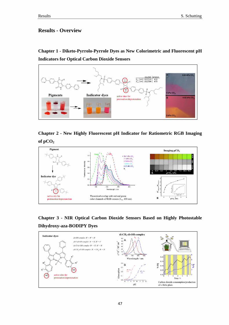
Results S. Schutting
47
Results - Overview
Chapter 1 - Diketo-Pyrrolo-Pyrrole Dyes as New Colorimetric and Fluorescent pH
Indicators for Optical Carbon Dioxide Sensors
Chapter 2 - New Highly Fluorescent pH Indicator for Ratiometric RGB Imaging
of pCO2
Chapter 3 - NIR Optical Carbon Dioxide Sensors Based on Highly Photostable
Dihydroxy-aza-BODIPY Dyes
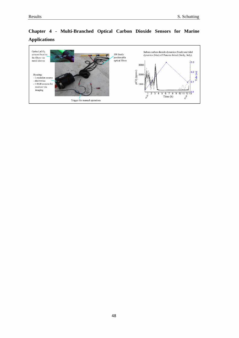
Results S. Schutting
48
Chapter 4 - Multi-Branched Optical Carbon Dioxide Sensors for Marine
Applications
Chapter 1 S. Schutting
49
Chapter 1
Scope of this chapter
Optical plastic type sensors consist of a pH-sensitive indicator dye and a base,
embedded in a polymer matrix and represent a promising alternative to the known
routine detection techniques of carbon dioxide. Up to now, state-of-the-art CO2 sensors
are almost exclusively based on the fluorescent pH-indicator 8-hydroxypyrene-1,3,6-
trisulfonate (HPTS).
Although HPTS features high fluorescence quantum yields (~1), good photostability, a
pKa value meeting the demands for physiological measurements and a large Stokes shift
(~60 nm in solution and ~50 nm embedded in ethyl cellulose), it suffers from different
drawbacks, such as only moderate absorption coefficients (24000 M-1cm-1) or
absorption and emission maxima at rather short wavelengths. Thus, ratiometric read-out
is only enabled, if the exciation wavelength is chosen in the UV region of the spectrum.
If this is not the case, addition of reference materials is required for reliable
measurements, but here, photobleaching of the indicator dye, the reference or both can
cause significant changes in the signals and the respective ratio.
In the following chapter a new indicator class based on diketo-pyrrolo-pyrroles is
presented. These dyes meet the requirements of high molar absorption coefficients, high
quantum yields for the protonated (neutral) forms, larger Stokes shifts than HPTS, good
photostability and absorption and emission spectra at higher wavelengths. Additionally,
they feature tuneable pKa values according to their substitution pattern. Hence, they
represent a promising alternative pH-sensitive indicator class to HPTS.
Despite these advantages, DPP indicators can be improved. Their sensitivity can be
further tuned to meet the users demands, their photostability could be improved, as well
as the quantum yields of the deprotonated (ionic) forms.

Chapter 1 S. Schutting
50

Chapter 1 S. Schutting
51
Diketo-Pyrrolo-Pyrrole Dyes as New Colorimetric and Fluorescent pH Indicators for Optical Carbon Dioxide Sensors
This chapter was published in Analytical Chemistry, 2013, 85, 3271- 3279; doi: 10.1021/ac303595v
Authors: Susanne Schutting, Sergey M. Borisov and Ingo Klimant
New indicators for optical CO2 sensors are synthesized in two steps from the
commercially available diketo-pyrrolo-pyrrole (DPP) pigments Irgazin Ruby and
Irgazin Scarlet. After introduction of bis(2-ethylhexyl) sulfonamide groups via a simple
two-step synthesis the pigments are rendered highly soluble in organic solvents and in
polymers and show pH-dependent absorption and emission spectra. The new indicators
have molar absorption coefficients in a 20000-50000 M-1cm-1 range, possess quantum
yields close to unity and feature good photostability. The indicators along with a
quaternary ammonium base are embedded into ethyl cellulose to give optical carbon
dioxide sensors. The absorption and emission spectra of the deprotonated form are
bathochromically shifted by more than 100 nm compared to the protonated form (λmax
absorption 496-550 nm; λmax emission 564-587 nm). This enables colorimetric read-out
and self-referenced ratiometric fluorescence intensity measurements. Importantly, the
dynamic range of the sensors based on the new indicators is significantly different (0-10
kPa and 1-100 kPa CO2) which enables a broad variety of applications.
Introduction
Carbon dioxide is one of the most important analytes on earth. Therefore its detection is
an important task in many fields, e.g. in biotechnology for controlling the fermentation
processes in bioreactors,92,93 in medicine for monitoring the CO2 content in patients
breath,61,94 in marine research for investigating long-term consequences of ocean
acidification for underwater flora and fauna9,95–98 and in food packaging for controlling
the gas content in modified atmosphere packaging.99 The Severinghaus electrode shows
Chapter 1 S. Schutting
52
linearity in a range between 1 kPa and 11 kPa,77 but it is not well applicable to measure
low pCO2 (e.g. the usual marine levels of about 0.04 kPa or 400 ppm), it suffers from
the electromagnetic interferences and can only be applied in aqueous solutions. IR
analyzers are robust and fast,61 but are mostly suitable for CO2 detection in gases85,86
since interference from water is very significant. On the other hand, optical CO2
chemosensors represent promising analytical tools which can be realized in the form of
fiber-optic sensors or planar optodes suitable for imaging applications.51 Most
colorimetric sensors rely on triphenylmethane dyes.57,89,100 The inner filter effect101–104
and Förster Resonance Energy Transfer (FRET)105,106 have been used to convert the
colorimetric sensors into the luminescence intensity-based ones. The read-out via
fluorescence intensity and high cross-sensitivity to oxygen are severe limitations of the
first and the second scheme, respectively. The latter also refers to a phosphorescent
carbon dioxide probe.107 One of the most popular fluorescent pH indicators for CO2
sensors is 8-hydroxypyrene-1,3,6-trisulfonate (HPTS).50 It is known for its high
fluorescence quantum yield of ~1,108,109 good photostability,64 and large Stokes´
shift.64,110 Thus, HPTS was used in numerous pCO2 sensors in a variety of applications.
So called plastic type sensors on HPTS basis (which typically make use of the indicator
and a quaternary ammonium base in a hydrophobic polymer or a sol-gel) are popular
due to the flexibility of formats, fast dynamic response and simplicity in
preparation,51,65,66,89,111–113 but those of Severinghaus type were also reported.114 The
disadvantages of HPTS include moderate molar absorption coefficients (24000 M-1cm-
1)115 and the fact that ratiometric measurement is only possible if the UV light is used
for the excitation. Several alternative sensing concepts have been proposed recently.
They explore the changes in the microenvironment during the carbamate formation
monitored with help of a microviscosity probe116 or aggregation-induced emission.117 In
a similar concept the change in microenvironment due to the protonation of an amidine
is detected via a solvatochromic probe.118 Notably, all these new probes operate at
rather high pCO2 and mostly rely on the measurements of fluorescence intensity, only
the probe reported by Wolfbeis and co-workers is suitable for ratiometric read-out.118
Diketo-pyrrolo-pyrrole (DPP) pigments were discovered in the 1980s and since that
time mainly used as low cost pigments for applications with high-quality demands.119,120
DPPs are applied in biophotonics and optoelectronics121 for preparation of low bandgap
conjugated polymers122–125 or copolymers used in semiconductors.126 Only a few
fluorescent probes based on DPP chromophores have been reported so far.127,128

Chapter 1 S. Schutting
53
Particularly Qu et al. proposed a fluoride probe based on deprotonation of the lactam in
the DPP chromophore which resulted in a bathochromic shift of the absorption and
emission spectra. We perceived that DPP chromophores could be suitable for designing
optical carbon dioxide sensors since they rely on an acid base equilibrium. In this study
we present a new alternative class of pH sensitive indicators for CO2 sensors, which are
based on diketo-pyrrolo-pyrrole dyes that are rendered highly soluble in organic
solvents and in polymers by introducing dialkyl sulfonamide groups. The indicators
show significantly different absorption and emission spectra for the neutral and
deprotonated form which enables colorimetric read-out and self-referenced ratiometric
fluorescence intensity measurements. The sensors also feature tunable sensitivity, large
relative signal change at low pCO2 and good photostability.
Experimental
Materials.
3,6-bis(1,1´-biphenyl)-2,5-dihydropyrrolo[3,4-c]pyrrole-1,4-dione (Irgazin Ruby), 3,6-
bis-phenyl-2,5-dihydropyrrolo[3,4-c]pyrrole-1,4-dione (Irgazin Scarlet), 1,6,7,12-
tetraphenoxy-N,N´-bis(2,6-diisopropylphenyl)-perylene-3,4:9,10-tertracarboxylic
bisimide (Lumogen-Red) and N,N´-bis(2,6-diisopropylphenyl)-perylene-3,4:9,10-
tertracarboxylic bisimide (Lumogen-Orange) were purchased from Kremer Pigments
(Germany, www.kremer-pigmente.com). The purity of these materials is confirmed by
the elementary analysis (Table S1 of the supporting information). Chlorosulfonic acid
has been received from Fluka (Sigma-Aldrich, www.sigmaaldrich.com). Ethyl cellulose
(EC49, ethoxyl content 49%), dimethylformamide (anhydrous), sodium sulfate
(anhydrous), triethylamine, sodium 8-hydroxy-pyrene-1,3,6-trifulfonate (HPTS),
tetrakis(decyl)ammonium hydroxide (TDA, 10% in methanol) and tetraoctylammonium
hydroxide solution (TOAOH, 20% in methanol) were obtained from Sigma-Aldrich.
The silicone components vinyl terminated polydimethylsiloxane (viscosity 1000 cSt.),
(25-35% methylhydrosiloxane)-dimethylsiloxane copolymer (viscosity 25-35 cSt.),
1,3,5,7-tetravinyl-1,3,5,7-tetramethylcyclotetrasiloxane, the platinum-
divinyltetramethyldisiloxane complex, anhydrous diethyl ether and bis(2-
ethylhexyl)amine were received from ABCR (Germany, www.abcr.de). Ultrafine
titanium dioxide P170 was purchased from Kemira (www.kemira.com). Nitrogen, 5%

Chapter 1 S. Schutting
54
carbon dioxide in nitrogen, 0.2% carbon dioxide in nitrogen and carbon dioxide (all of
99.999% purity) were obtained from Air Liquide (Austria, www.airliquide.at).
HPTS(TOA)3 was prepared as reported previously.112 Toluene, tetrahydrofuran (THF),
ethanol and hexane were purchased from VWR (Austria, www.vwr.com). Poly(ethylene
terephthalate) (PET) support Melinex 505 was obtained from Pütz (Germany,
www.puetz-folien.com). Silica-gel, as well as the buffer salts 2-(cyclohexylamino)-
ethansulfonic acid (CHES) and cyclohexylaminopropansulfonic acid (CAPS) were
received from Roth (www.carlroth.com). For HPLC experiments methanol picograde
was purchased from LGC Standards (www.lgcstandards.com) and de-ionized water was
filtered via a Barnstead NANOpure ultrapure water system for HPLC experiments.
Synthesis of 3,6-bis[4´(3´)-disulfo-1,1´-biphenyl-4-yl]-2,5-dihydropyrrolo[3,4-
c]pyrrole-1,4-dione dipotassium salt (1).
Irgazin Ruby (1 g, 2.3 mmol) was stirred in chlorosulfonic acid (10 ml, 150 mmol) for 4
h at 60 °C. The mixture was cooled to ambient temperature, pipetted on ice and washed
with cold deionized water until reaching a neutral pH. The centrifuged sediment was
then hydrolyzed in 250 ml of a mixture of deionized water (180 ml), acetone (30 ml)
and dimethylformamide (40 ml) and potassium carbonate was added until reaching a
slightly basic pH. After the solvent mixture was evaporated under reduced pressure, the
crude product was dissolved in a mixture of water:methanol (HPLC grade, 1:1) and
purified via semi-preparative high performance liquid chromatography eluting isocratic
with a H2O:MeOH (55:45) to obtain a dark violet powder of 1. Matrix assisted laser
desorption/ionization – time of flight (MALDI-TOF) for 1: m/z of [MH]+ found 676.99,
calculated 676.99; m/z of [MK]+ found 714.94, calculated 714.94. 1H NMR spectra
indicate formation of a mixture of isomers containing sulfo-groups in position 5 and 6
of the biphenyl.
Synthesis of 3,6-bis[4´-bis(2-ethylhexyl)sulfonylamide-1,1´-biphenyl-4-yl]-2,5-
dihydropyrrolo[3,4-c]pyrrole-1,4-dione (2).
Irgazin Ruby (1 g, 2.3 mmol) was stirred in chlorosulfonic acid (7 ml, 105 mmol) for 3
h at 60 °C. The mixture was cooled to ambient temperature, pipetted on ice and washed
with cold de-ionized water until reaching a neutral pH. The sediment was collected via

Chapter 1 S. Schutting
55
centrifugation and was washed three times with diethyl ether:tetrahydrafurane (10:1).
The sediment was dissolved in anhydrous dimethylformamide (50 ml) and bis(2-
ethylhexyl)amine (4 ml, 13 mmol) and triethylamine (3 ml, 22 mmol) were added. The
mixture was stirred overnight at ambient temperature, diluted with deionized water and
neutralized with acetic acid. The dye was extracted with dichloromethane, hydrochloric
acid, ethanol and sodium chloride where added to facilitate the phase separation. The
organic phase was collected, dried over anhydrous sodium sulfate and evaporated to
dryness under reduced pressure. The crude product was purified via column
chromatography on silica gel using toluene/tetrahydrofuran (95:5). The product was
dissolved in dichloromethane and precipitated with hexane to give a dark red powder
(0.69 g, 29% of theoretical yield of 2). MALDI-TOF: m/z of [MH]+ found 1047.6,
calculated 1047.6. 1H NMR (300MHz, CDCl3) δ 8.46 (s, 4H), 7.81 (m, 4H), 7.69 (m,
8H), 3.06-2.88 (m, 8H), 1.61 (s, 4H), 1.26-1.21 (m, 32H), 0.85-0.80 (m, 24H). Analysis
for C62H86S2N4O6 found: C68.96, H7.28, N7.11, calculated: C69.00, H7.66, N7.10.
Synthesis of 3-(phenyl)-6-(4-bis(2-ethylhexyl)sulfonylamide-phenyl)-2,5-
dihydropyrrolo[3,4-c]pyrrole-1,4-dione (3) and 3,6-bis[4-bis(2-
ethylhexyl)sulfonylamide-phenyl]-2,5-dihydropyrrolo[3,4-c]pyrrole-1,4-dione (4).
Irgazin Scarlet (2 g, 6.9 mmol) was dispersed in the mixture of sulfuryl chloride (2 ml,
24 mmol) and chlorosulfonic acid (6 ml, 90 mmol) and was stirred for 12 h at 65 °C.
The protocol used for the preparation of 2 was followed, but 10 ml (33 mmol) of bis(2-
ethylhexyl)amine and 4 ml (29 mmol) triethylamine were used instead. The crude
products were purified via column chromatography on silica gel eluting with a gradient
of toluene:acetone (75:25) to obtain 3 and 97:3 to obtain 4. The products were
recrystallized from n-butanol to give 3 as dark red crystals (0.54 g, 13% of theoretical
yield of 3) and 4 as an orange powder (0.4 g, 6% of theoretical yield of 4). MALDI-
TOF for 3: m/z of [MH]+ found 592.3214, calculated 592.3209. 1H NMR (300MHz,
DMSO-d6) δ 8.52 (s, 1H), 8.46 (t, 2H), 8.34 (dd, 2H), 7.87 (d, 2H), 7.84-7.69 (m, 2H),
2.95 (m, 4H), 1.57 (m, 2H), 1.44-1.08 (m, 16H), 0.85 (m, 12H). Analysis for
C34H45SN3O4 (3) found: C 70.66, H 8.09, N 5.29, calculated: C 71.09, H 8.28, N 5.35.
MALDI-TOF for 4: m/z of [MH]+ found 895.5469, calculated 895.5441. 1H NMR
(300MHz, CDCl3) δ 8.43 (d, 4H), 7.82 (m, 4H), 2.98-2.89 (m, 8H), 1.55 (m, 4H), 1.44-
Chapter 1 S. Schutting
56
1.01 (m, 32H), 0.84 (m, 24H). Analysis for C50H78S2N4O6 (4) found: C 67.24, H 8.65, N
6.12, calculated: C 67.08, H 8.78, N 6.26.
Preparation of the Sensing Foils.
“Cocktail 1” containing X mg dye and 100 µl tetraoctylammonium hydroxide solution
(20% TOAOH in MeOH) was purged with carbon dioxide gas. “Cocktail 2” containing
200 mg ethyl cellulose dissolved in 3800 mg of a toluene:ethanol mixture (6:4) was
added to the “cocktail 1”. For the absorption measurements X was 2.4 mg (1.2%w/w in
respect to the polymer) in case of 2 and 3.0 mg (1.5%w/w) for 3 and 4. For the emission
measurements X was 0.8 mg (0.4%w/w) for 2 and 0.5 mg (0.25%w/w) for 3 and 4. The
resulting mixture was knife-coated on a dust-free PET support. A sensing film of ~7.5
µm thickness was obtained after evaporation of the solvent. The sensing film was
covered with a gas-permeable ~22 µm thick silicone layer by knife-coating “cocktail 3”
consisting of 800 mg vinyl terminated polydimethylsiloxane, 32 µl (25-35%
methylhydrosiloxane)-dimethylsiloxane copolymer, 2 µl 1,3,5,7-tetravinyl-1,3,5,7-
tetramethylcyclotetrasiloxane and 4 µl platinum-divinyltetramethyldisiloxane complex
dissolved in 1600 mg hexane. For emission measurements a similar layer was prepared
but 200 mg of titanium dioxide were dispersed in “cocktail 3”. The silicon layers were
kept in an oven (60 °C) for 10-15 min to complete polymerization.
Methods. 1H NMR spectra were recorded on a 300 MHz instrument (Bruker) in CDCl3 and
DMSO-d6 with TMS as standard. Absorption spectra were recorded on a Cary 50 UV-
Vis Spectrophotometer (www.varianinc.com). The determination of the molar
absorption coefficients was carried out as an average of 3 independent measurements.
Fluorescence spectra were recorded on a Hitachi F-7000 fluorescence spectrometer
(www.hitachi.com) equipped with a red-sensitive photomultiplier R928 from
Hamamatsu (www.hamamatsu.com). The relative fluorescence quantum yields were
determined according to Demas and Crosby.129 The solutions of Lumogen-Orange (Φ ≈
1) and Lumogen-Red (Φ ≈ 0.96)130,131 in chloroform were used as standards for the
protonated and the deprotonated form, respectively. The absolute fluorescence quantum
yields were determined on a Fluorolog3 fluorescence spectrometer (www.horiba.com)
equipped with a NIR-sensitive photomultipier R2658 from Hamamatsu (300-1050 nm)
Chapter 1 S. Schutting
57
and an integrating sphere (Horiba). Three independent measurements were performed
for determination of the relative and the absolute quantum yields and the average value
obtained in the two methods was used. In case of the sensing materials only the absolute
quantum yields were determined. Photobleaching experiments were performed by
irradiating the samples (2.5 ml) with the light of a high-power 10 W LED array (λmax
458 nm, 3 LEDs, www.led-tech.de) operated at 6 W input power. A lens (Edmund
optics, www.edmundoptics.de) was used to focus the light of the LED array on the glass
cuvette (photon flux: ∼4600 µmol⋅s-1⋅m2 as determined with a Li-250A light meter from
Li-COR, www.licor.com). The photodegradation profiles were obtained by monitoring
the absorption spectra of the respective dye dissolved in tetrahydrofuran. For
experiments with ratiometric read-out a two-phase lock-in amplifier (SR830,
www.thinksrs.com) and a home-made device consisting of two separate detection
channels, which was described previously in detail,132 were used. Each detection
channel was equipped with a photomultiplier module H9306-02 from Hamamatsu. A
450 nm LED (www.roithner-laser.com) combined with a short-pass BG-12 filter served
as an excitation source. The emission of the neutral form was filtered through HC
562/40 band-pass filter (www.ahf.de) and an RG-630 long-pass filter from Schott was
used for the deprotonated form. A four-armed optical filter bundle (www.leoni-fiber-
optics.com) was used to guide the excitation light to the sensing foil and to guide back
the emission to the two detection channels. Gas calibration mixtures were obtained
using a gas mixing device from MKS (www.mksinst.com). The gas mixture was
humified to about 100% relative humidity prior entering the calibration chamber.
Temperature was controlled by a cryostat ThermoHaake DC50. Semi-preparative HPLC
was performed on a Knauer Smartline Instrument with Autosampler 3800 (Manager
5000, Pump 1000, UV Diode Array Detector 2600 and Fraction Collector Teledyne Isco
Foxy Jr. FC100 modules) equipped with a Machery-Nagel VP 125/21 Nucleodur 100-5
C18 ec column (internal diameter: 21.0mm) with a VP 20/16 Nucleodur C18 ec pre-
column at a flow rate of 13ml/min. The pH of the buffer solutions (CHES and CAPS)
was controlled by a digital pH meter (InoLab pH/ion, www.wtw.com) calibrated at 25
°C with standard buffers of pH 7.0 and pH 4.0 (www.wtw.com). The buffers were
adjusted to constant ionic strength (IS = 0.05 M) using sodium chloride as the
background electrolyte.

Chapter 1 S. Schutting
58
Results and Discussion
Synthesis.
We expected the diketo-pyrrolo-pyrrole chromophore to be pH-sensitive due to the
deprotonation of the lactam ring. Preliminary experiments with suspensions of DPP
pigments confirmed this hypothesis. However, DPP pigments are known to have planar
structure and possess very poor solubility in the organic solvents.133 In fact the DPP
dyes are mostly applied as non-soluble pigments in paints. The low solubility prevents
the dyes from application as indicators in optical sensors. Typically, the DPP pigments
are rendered soluble by an alkylation of the lactam nitrogen atoms134 but this
modification is of course not suitable for preparation of pH indicators. A water-soluble
disulfonate 1 (Scheme 1.1) was prepared via chlorosulfonation of the commercially
available pigment Irgazin Ruby (Pigment Red 264) and subsequent hydrolysis of the
product in aqueous medium. This dye was found to be pH sensitive and was used for the
estimation of the pKa (see below). A simple 2-step strategy was established to convert
the DPP pigments into lipophilic pH indicators highly soluble in organic solvents and
polymers (Scheme 1.1) and thus to make the dyes suitable for application in plastic
carbon dioxide sensors. Two different pigments containing phenyl or biphenyl
substituents in the 3,6 position of the DPP were used. The chloro-sulfonation (first step)
was carried out with large excess of chlorosulfuric acid to prevent possible hydrolysis
during sulfonation. The chlorosulfonation of Irgazin Scarlet (Pigment Red 255, DPP)
proved to be more difficult than for Irgazin Ruby and required addition of sulfuryl
chloride to achieve acceptable yields. To minimize the formation of side products due to
hydrolysis the second step (reaction with a branched secondary amine) was performed
without thorough purification of the chlorosulfonated intermediate.
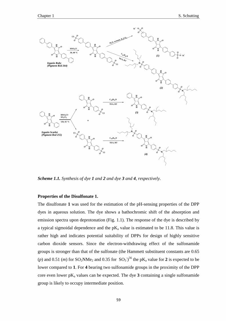
Chapter 1 S. Schutting
59
HN
NH
O
O
HN
NH
O
O
HSO3Cl
3h, 60 °C
S
S
O
O
Cl
O
O
ClHN
NH
O
O
S
S
O
O
O
O
O
O
K+
K+
TEA, RT
H 2O, acetone, K 2C
O3
(2)
(1)
HN
NH
O
O
HSO3Cl+SO2Cl2
12h, 65 °C
HN
NH
O
O
SO
O
Cl
HN
NH
O
O
S
S
O
O
Cl
O
O
Cl
+
HN
NH
O
O
SO
O
HN
NH
O
O
S
S
O
O
O
O
HN
NH
O
O
S
S
O
O
N
O
O
N
C16H
35N
N
N
N
(3)
(4)
C16H35N
TEA, RT
C16H35N
TEA, RT
Irgazin Ruby(Pigment Red 264)
Irgazin Scarlet(Pigment Red 255)
Scheme 1.1. Synthesis of dye 1 and 2 and dye 3 and 4, respectively.
Properties of the Disulfonate 1.
The disulfonate 1 was used for the estimation of the pH-sensing properties of the DPP
dyes in aqueous solution. The dye shows a bathochromic shift of the absorption and
emission spectra upon deprotonation (Fig. 1.1). The response of the dye is described by
a typical sigmoidal dependence and the pKa value is estimated to be 11.8. This value is
rather high and indicates potential suitability of DPPs for design of highly sensitive
carbon dioxide sensors. Since the electron-withdrawing effect of the sulfonamide
groups is stronger than that of the sulfonate (the Hammett substituent constants are 0.65
(p) and 0.51 (m) for SO2NMe2 and 0.35 for SO3-)56 the pKa value for 2 is expected to be
lower compared to 1. For 4 bearing two sulfonamide groups in the proximity of the DPP
core even lower pKa values can be expected. The dye 3 containing a single sulfonamide
group is likely to occupy intermediate position.
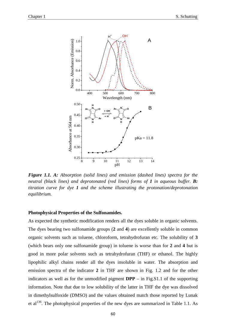
Chapter 1 S. Schutting
60
400 500 600 700 8000.0
0.2
0.4
0.6
0.8
1.0
8 9 10 11 12 13 140.25
0.30
0.35
0.40
0.45
0.50B
Nor
m. A
bsor
bance
(E
mis
sion
)
Wavelength (nm)
H+ OH-
A
Abs
orba
nce a
t 564
nm
pH
pKa = 11.8
NH
NH
O
O
Ar
Ar
N-
NH
O
O Ar
Ar+ OH
-
+ H+
Figure 1.1. A: Absorption (solid lines) and emission (dashed lines) spectra for the neutral (black lines) and deprotonated (red lines) forms of 1 in aqueous buffer. B: titration curve for dye 1 and the scheme illustrating the protonation/deprotonation equilibrium.
Photophysical Properties of the Sulfonamides.
As expected the synthetic modification renders all the dyes soluble in organic solvents.
The dyes bearing two sulfonamide groups (2 and 4) are excellently soluble in common
organic solvents such as toluene, chloroform, tetrahydrofuran etc. The solubility of 3
(which bears only one sulfonamide group) in toluene is worse than for 2 and 4 but is
good in more polar solvents such as tetrahydrofuran (THF) or ethanol. The highly
lipophilic alkyl chains render all the dyes insoluble in water. The absorption and
emission spectra of the indicator 2 in THF are shown in Fig. 1.2 and for the other
indicators as well as for the unmodified pigment DPP – in Fig.S1.1 of the supporting
information. Note that due to low solubility of the latter in THF the dye was dissolved
in dimethylsulfoxide (DMSO) and the values obtained match those reported by Lunak
et al136. The photophysical properties of the new dyes are summarized in Table 1.1. As
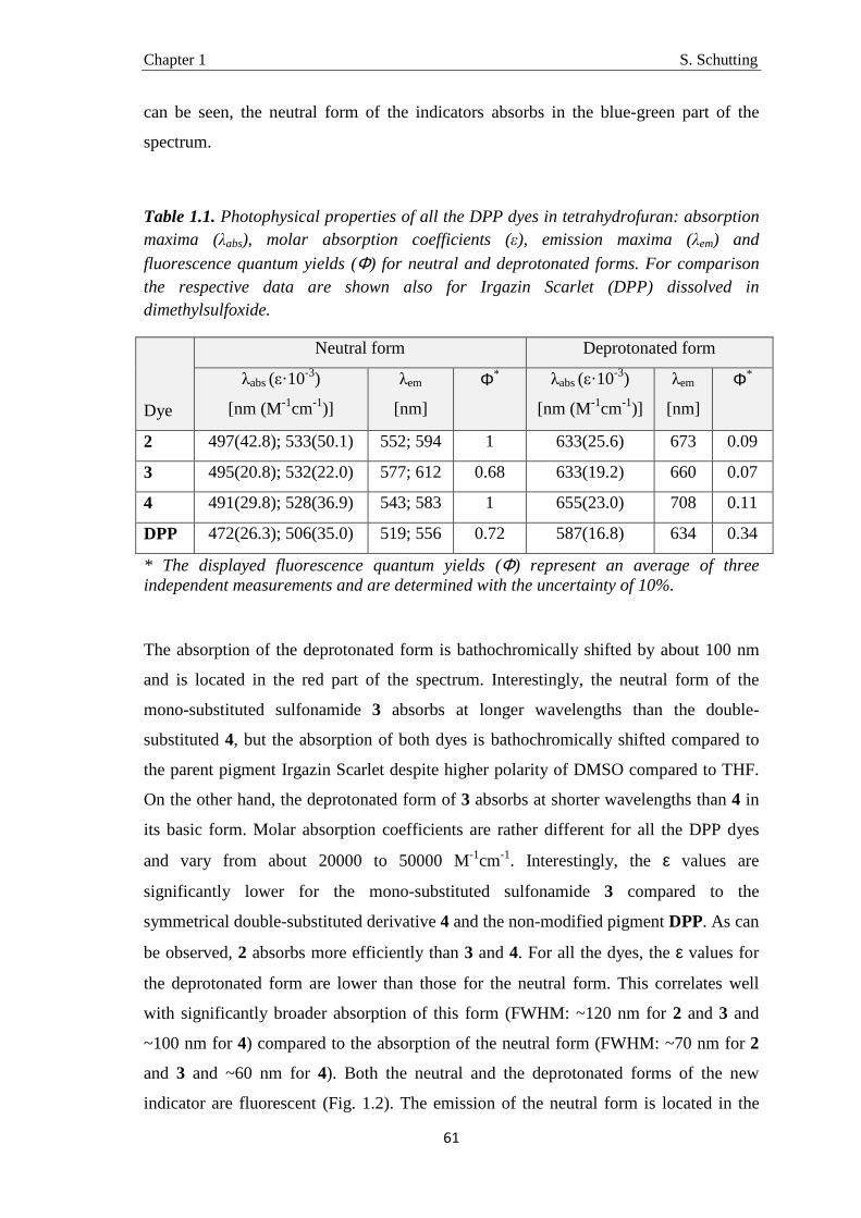
Chapter 1 S. Schutting
61
can be seen, the neutral form of the indicators absorbs in the blue-green part of the
spectrum.
Table 1.1. Photophysical properties of all the DPP dyes in tetrahydrofuran: absorption maxima (λabs), molar absorption coefficients (ε), emission maxima (λem) and
fluorescence quantum yields (Φ) for neutral and deprotonated forms. For comparison the respective data are shown also for Irgazin Scarlet (DPP) dissolved in dimethylsulfoxide.
Dye
Neutral form Deprotonated form
λabs (ε·10-3)
[nm (M-1cm-1)]
λem
[nm]
Φ*
λabs (ε·10-3)
[nm (M-1cm-1)]
λem
[nm]
Φ*
2 497(42.8); 533(50.1) 552; 594 1 633(25.6) 673 0.09
3 495(20.8); 532(22.0) 577; 612 0.68 633(19.2) 660 0.07
4 491(29.8); 528(36.9) 543; 583 1 655(23.0) 708 0.11
DPP 472(26.3); 506(35.0) 519; 556 0.72 587(16.8) 634 0.34
* The displayed fluorescence quantum yields (Φ) represent an average of three independent measurements and are determined with the uncertainty of 10%.
The absorption of the deprotonated form is bathochromically shifted by about 100 nm
and is located in the red part of the spectrum. Interestingly, the neutral form of the
mono-substituted sulfonamide 3 absorbs at longer wavelengths than the double-
substituted 4, but the absorption of both dyes is bathochromically shifted compared to
the parent pigment Irgazin Scarlet despite higher polarity of DMSO compared to THF.
On the other hand, the deprotonated form of 3 absorbs at shorter wavelengths than 4 in
its basic form. Molar absorption coefficients are rather different for all the DPP dyes
and vary from about 20000 to 50000 M-1cm-1. Interestingly, the ε values are
significantly lower for the mono-substituted sulfonamide 3 compared to the
symmetrical double-substituted derivative 4 and the non-modified pigment DPP. As can
be observed, 2 absorbs more efficiently than 3 and 4. For all the dyes, the ε values for
the deprotonated form are lower than those for the neutral form. This correlates well
with significantly broader absorption of this form (FWHM: ~120 nm for 2 and 3 and
~100 nm for 4) compared to the absorption of the neutral form (FWHM: ~70 nm for 2
and 3 and ~60 nm for 4). Both the neutral and the deprotonated forms of the new
indicator are fluorescent (Fig. 1.2). The emission of the neutral form is located in the

Chapter 1 S. Schutting
62
yellow-orange part of the spectrum and is very strong. In fact, the fluorescence quantum
yields Φ for the symmetrical double-substituted sulfonamides 2 and 4 are close to unity.
The fluorescence of the neutral form of 3 is less efficient (Φ = 0.68). The Stokes´ shifts
are rather small for symmetrical 2 and 4 (19 nm and 15 nm, respectively) and are
slightly larger for 3 (35 nm). However, this is of less relevance for the sensing
applications since very efficient excitation in the second band (located about 30 nm
shorter than the most intense absorption band) is possible for all the indicators. In
solutions the fluorescence of the deprotonated form is much weaker than that of the
neutral form (Φ = 0.07-0.11, Table 1.1).
400 500 600 700 8000.0
0.2
0.4
0.6
0.8
1.0OH-H+
Norm
. A
bso
rbance
&
Em
issi
on
Wavelength (nm)
Figure 1.2. Absorption (solid lines) and emission (dashed lines) spectra for the neutral (black lines) and deprotonated (red lines) forms of 2 in tetrahydrofuran.
Photostability.
Photobleaching experiments were carried out for the THF solutions of the dyes. A high
power blue LED array (λmax 458 nm) was used for the excitation of the neutral form. 8-
hydroxy-pyrene-1,3,6-trisulfonate in its lipophilic tetraoctylammonium ion pair
(HPTS(TOA)3) which is the most common state-of-the-art indicator for plastic carbon
dioxide sensors was used for comparison. The photodegradation profiles are displayed
in fig. S1.2. All DPP dyes showed significantly better photostability than HPTS(TOA)3.
The photostability of the doubly-substituted sulfonamides 2 and 4 was much higher than
for the mono-substituted 3 which correlates well both to the amount of electron-
withdrawing sulfonamide groups and the fluorescence quantum yields. Therefore, it can

Chapter 1 S. Schutting
63
not be concluded whether lower photostability of 3 compared to that for 2 and 4 is due
to higher probability of photooxidation processes (due to higher electron density on the
DPP core) or the photodegradation pathways involving the formation of the triplet
states.
Carbon Dioxide Sensors.
The indicators along with tetraoctylammonium hydroxide were embedded in ethyl
cellulose to obtain plastic carbon dioxide sensors. Clearly, the sensors respond to carbon
dioxide in altering their color (blue in the absence of CO2 and pink in the presence of
CO2) which enables colorimetric detection of carbon dioxide (Fig. 1.3).
Figure 1.3. Photographic images of the planar optode based on 2 in EC49 under ambient air and a flux of 5 kPa carbon dioxide: (A) under ambient light; (B) in the darkness under UV light (365 nm).
Distinct changes in the fluorescence color (from deep red to orange) are also evident.
Fig. 1.4 and Fig. S1.3 show the absorption and the emission spectra of the sensing
materials based on 2-4. Although the major trends established for THF solutions are
preserved also in the solid state sensors it is evident that the absorption of the
deprotonated form becomes narrower compared to the solutions. A shoulder in the
absorption spectrum at about 560 nm is also clearly visible. The presence of several
isosbestic points indicates that only two forms of an indicator are present in the acid-
base equilibrium.
Importantly, the fluorescence quantum yields of the deprotonated form nearly double in
ethyl cellulose (Table 1.2) and reach ∼0.2 which enables sufficient signal for the
ratiometric measurements. For all the sensors the fluorescence emission intensities for

Chapter 1 S. Schutting
64
both the neutral and the deprotonated form were increasing with CO2 concentration
(Fig. 1.4, Fig S1.3). The increase in the intensity of the deprotonated form is explained
by more efficient absorption of the neutral form at the excitation wavelength (e.g. λexc
505 nm for 2) and rather efficient Förster Resonance Energy Transfer (FRET) at this
dye concentration (0.4% w/w for 2). This is due to very good overlap between the
emission of the neutral form and the absorption of the deprotonated form. FRET may
also be the reason for lower quantum yields determined in ethyl cellulose for the neutral
form of the dyes compared to the solution measurements (Tables 1.1 and 1.2).
Table 1.2. Photophysical properties of all the DPP dyes in ethyl cellulose film (EC49): absorption maxima (λabs), molar absorption coefficients (ε), emission maxima (λem) and
fluorescence quantum yields (Φ) for the neutral and deprotonated forms.
Dye
Neutral form Deprotonated form
λabs
[nm]
λem
[nm]
Φ
λabs
[nm]
λem
[nm]
Φ
2 505; 541 565 0.64 606 653 0.19
3 516; 550 587 0.64 597 641 0.18
4 496; 534 564 1 615 682 0.17
As can be seen (Fig. S1.4) dye concentration barely affects the colorimetric read-out but
is crucial for the emission measurements due to FRET. In fact, in case of high dye
concentration (1.2% w/w) the emission spectrum is dominated by the deprotonated form
at pCO2 below 5 kPa. On the other hand, in case of low dye concentration the neutral
form clearly dominates the emission at this pCO2 (Fig. S1.4). Thus, the dynamic range
of the sensing materials using emission read-out can be tuned by adjusting the
concentration of the indicators. Fig. 1.4 also shows the respective calibration plots for
the sensors based on 2-4. Despite rather different structure of 2 and 3 the sensors show
comparable sensitivity. Both sensors operate in the dynamic range from 0 to 10 kPa
CO2 and retain dynamics at atmospheric pCO2 of 0.04 kPa. At lower carbon dioxide
levels it is very difficult to ensure that the system (flow through cell, gas mixing device,
connectors etc.) is completely decarbonated and thus some contamination with CO2 can
be observed. In fact, the experimental values at very low pCO2 deviate from the
expected linear dependence (Fig. S1.5). Therefore, determination of the Limit of
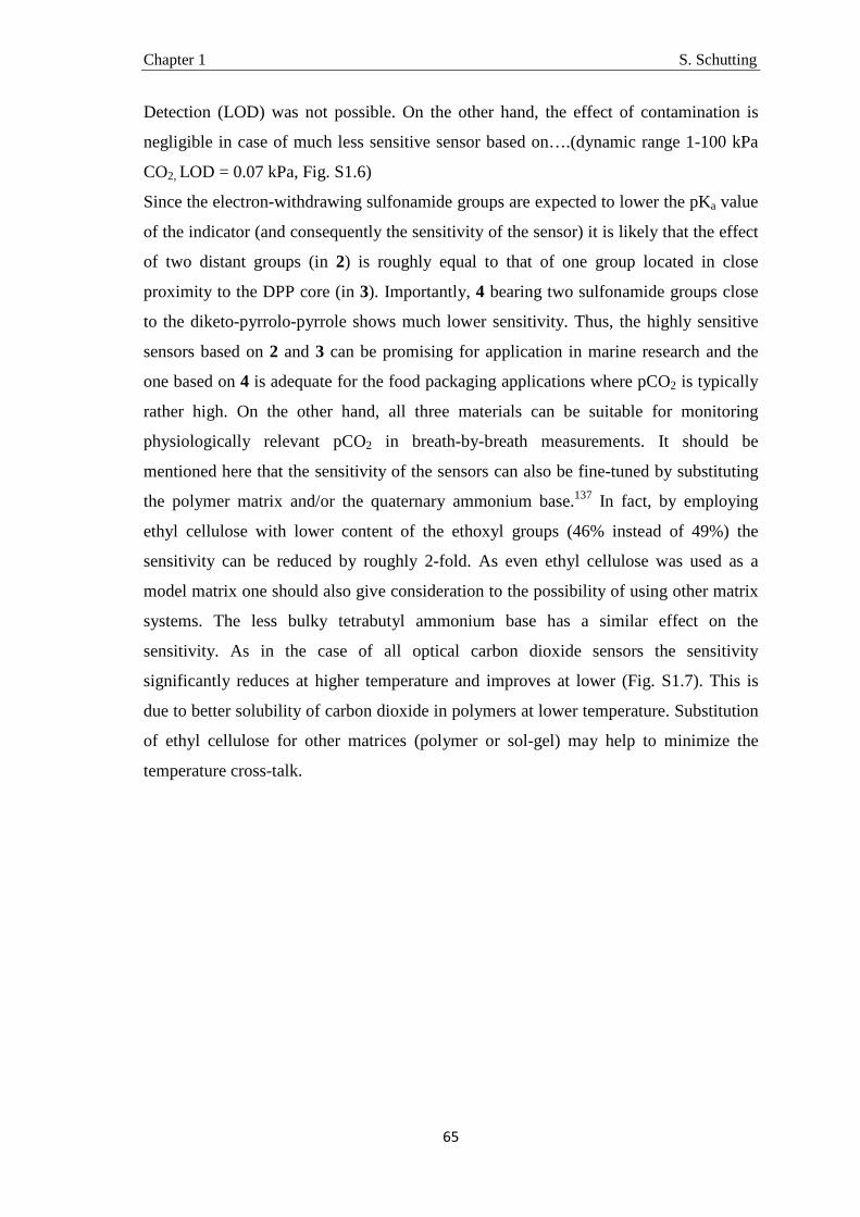
Chapter 1 S. Schutting
65
Detection (LOD) was not possible. On the other hand, the effect of contamination is
negligible in case of much less sensitive sensor based on….(dynamic range 1-100 kPa
CO2, LOD = 0.07 kPa, Fig. S1.6)
Since the electron-withdrawing sulfonamide groups are expected to lower the pKa value
of the indicator (and consequently the sensitivity of the sensor) it is likely that the effect
of two distant groups (in 2) is roughly equal to that of one group located in close
proximity to the DPP core (in 3). Importantly, 4 bearing two sulfonamide groups close
to the diketo-pyrrolo-pyrrole shows much lower sensitivity. Thus, the highly sensitive
sensors based on 2 and 3 can be promising for application in marine research and the
one based on 4 is adequate for the food packaging applications where pCO2 is typically
rather high. On the other hand, all three materials can be suitable for monitoring
physiologically relevant pCO2 in breath-by-breath measurements. It should be
mentioned here that the sensitivity of the sensors can also be fine-tuned by substituting
the polymer matrix and/or the quaternary ammonium base.137 In fact, by employing
ethyl cellulose with lower content of the ethoxyl groups (46% instead of 49%) the
sensitivity can be reduced by roughly 2-fold. As even ethyl cellulose was used as a
model matrix one should also give consideration to the possibility of using other matrix
systems. The less bulky tetrabutyl ammonium base has a similar effect on the
sensitivity. As in the case of all optical carbon dioxide sensors the sensitivity
significantly reduces at higher temperature and improves at lower (Fig. S1.7). This is
due to better solubility of carbon dioxide in polymers at lower temperature. Substitution
of ethyl cellulose for other matrices (polymer or sol-gel) may help to minimize the
temperature cross-talk.

Chapter 1 S. Schutting
66
400 450 500 550 600 6500.0
0.2
0.4
0.6
0.8
1.0
550 600 650 700 750 8000.0
0.2
0.4
0.6
0.8
1.0
0 1 2 3 4 5024
68
101214
0 1 2 3 4 5
0.0
0.5
1.0
1.5
0 5 10 15 20 25 30 350
5
10
15
20
0 5 10 15 20 25 30 35
0.2
0.4
0.6
0.8
1.0
1.2C
B
Nor
m.
Abso
rbanc
e
Wavelength (nm)
pCO2 (kPa)00.49
1.964.91
A∆λ∆λ∆λ∆λ2
Norm
. E
mis
sion
Wavelength (nm)
pCO2 (kPa)
00.491.964.91
∆λ∆λ∆λ∆λ1
pCO2 (kPa)
4
2
Ratio
Aneu
tra
l/Adep
rot
F
E
pCO2 (kPa)
Ratio
I neu
tra
l/Idep
rot
4
2
D
4
3
Ratio
Aneu
tra
l/Adep
rot
pCO2 (kPa)
ABSORBANCE EMISSION
4
3
pCO2 (kPa)
Ratio
I neu
tral/
I de
prot
Figure 1.4. Absorption (A) and emission (D) spectra for the carbon dioxide sensor based on 2 (25 °C). Calibration curves for the sensors based on 2-4: the ratio of
absorption (B and C) and fluorescence intensity (E and F) in the λmax of the absorption
and emission spectra (λexc 505 nm for 2, 510 nm for 3 and 495 nm for 4), respectively, of the neutral and deprotonated forms of the indicators (25 °C).
Comparison of the Optical and Sensing Properties with State-of-the-art Sensors.
Since HPTS is one of the most frequently used fluorescent pH indicators for CO2
sensors a comparison between the sensors based on this indicator and the new DPP
indicators is interesting. Generally, the new indicators and HPTS show comparable
molar absorption coefficients. The fluorescence quantum yields of the neutral form of
the DPP indicators are comparable to the Φ for HPTS but the deprotonated forms of the
former possess lower brightness. The 2-wavelength absorption/reflectance
measurements are possible for both indicator classes, but for DPPs the wavelength is
significantly longer. In fact, the absorption maximum of the protonated form of HPTS is
located in the UV region (395 nm). The DPPs are excellently suitable for ratiometric
emission measurements under blue excitation, whereas only unreferenced
measurements of fluorescence intensity are possible for HPTS under the same
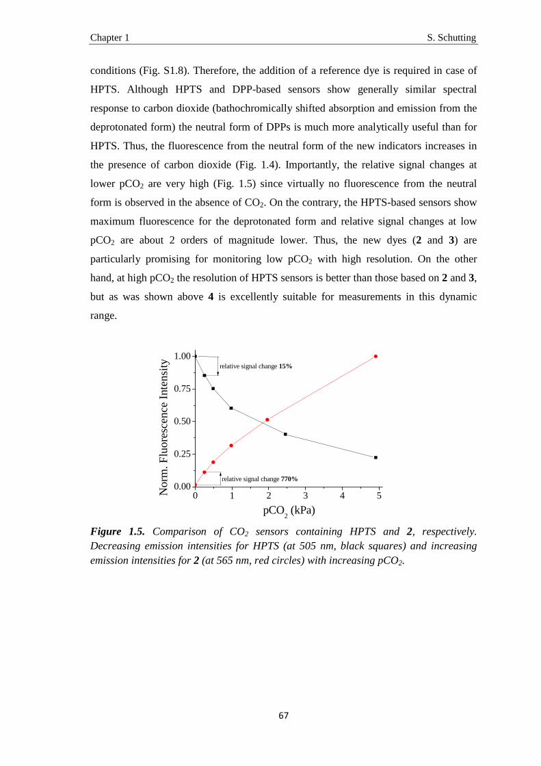
Chapter 1 S. Schutting
67
conditions (Fig. S1.8). Therefore, the addition of a reference dye is required in case of
HPTS. Although HPTS and DPP-based sensors show generally similar spectral
response to carbon dioxide (bathochromically shifted absorption and emission from the
deprotonated form) the neutral form of DPPs is much more analytically useful than for
HPTS. Thus, the fluorescence from the neutral form of the new indicators increases in
the presence of carbon dioxide (Fig. 1.4). Importantly, the relative signal changes at
lower pCO2 are very high (Fig. 1.5) since virtually no fluorescence from the neutral
form is observed in the absence of CO2. On the contrary, the HPTS-based sensors show
maximum fluorescence for the deprotonated form and relative signal changes at low
pCO2 are about 2 orders of magnitude lower. Thus, the new dyes (2 and 3) are
particularly promising for monitoring low pCO2 with high resolution. On the other
hand, at high pCO2 the resolution of HPTS sensors is better than those based on 2 and 3,
but as was shown above 4 is excellently suitable for measurements in this dynamic
range.
0 1 2 3 4 50.00
0.25
0.50
0.75
1.00
relative signal change 770%
Norm
. F
luore
scence
Int
ensi
ty
pCO2 (kPa)
relative signal change 15%
Figure 1.5. Comparison of CO2 sensors containing HPTS and 2, respectively. Decreasing emission intensities for HPTS (at 505 nm, black squares) and increasing emission intensities for 2 (at 565 nm, red circles) with increasing pCO2.

Chapter 1 S. Schutting
68
Sensor Response Times and Reproducibility.
The dynamic response was estimated by abruptly changing the pCO2 from 0.25 kPa to
4.91 kPa and back for 2 and 3 and from 4.91 kPa to 98.13 kPa and back for 4. The t90
time (time needed for 90% of the signal change to occur) was estimated to be about 90 s
and about 40 s for the response and recovery, respectively. Evidently, the response and
recovery times are influenced by the thickness of the sensing layer and the thickness of
the silicon layer. The thicknesses of both can be reduced to enable faster response,
however higher concentration of the indicator will be necessary to ensure sufficient S/N
ratio. The dynamic range of the material is expected to shift due to more efficient FRET
at higher dye concentration albeit only for the fluorescence measurements. Evidently,
increasing the dye concentration will not significantly influence the dynamic range upon
colorimetric measurement. To demonstrate the reproducibility of the sensors we
performed prolong measurements with alternating pCO2 using 450 nm LED for the
excitation and detecting fluorescence in 2 channels: 542-582 nm for isolating the
emission of the neutral form and >630 nm for the basic form, respectively. The ratio of
the intensities in the two channels served as an analytical parameter. All the sensors
show highly reproducible response without a noticeable drift (Fig. 1.6, Fig. S1.9 and
S1.10). Importantly, the sensors based on 2 and 3 show excellent photostability (no
degradation of fluorescence intensity for the neutral and deprotonated forms) even
within several hours of continuous excitation. In case of 4 a very minor drift due to
photobleaching is observed after 5 h of continuous read-out. Importantly,
photobleaching of the indicator reduces its concentration and therefore FRET efficiency
which can result in the drift of calibration plots. However it should be mentioned here
that we used continuous irradiation in order to access the photostability. Typically, a
short pulse of 100 ms is more than sufficient to access the fluorescence intensity in both
channels and the acquisition will be performed once in several seconds. Thus, the
operating lifetime of the sensors can be extended by several orders of magnitude.
Comparison with the sensors based on HPTS(TOA)3 reveal rather strong drift due to
significantly faster photobleaching of the dye in identical conditions (Fig. S1.11).
Chapter 1 S. Schutting
69
0.0 0.5 1.0 1.5 2.0 2.5 3.0
50
100
150
0.0 0.5 1.0 1.5 2.0 2.5 3.00.0
0.5
1.0
1.5
2.0
4.91 kPa
Flu
ores
cence
Int
ensi
ty (
a.u.)
Time (h)
0.25 kPa
Rat
io I n
eutr
al/I d
epro
t
Time (h)
4.91 kPa
0.25 kPa
Figure 1.6. Above: Fluorescence intensity for the neutral (black line) and deprotonated (red line) forms of 2 (up) and Below: calculated ratio Ineutral/Ideprot (down) for pCO2 alternating between 0.25 kPa and 4.91 kPa under continuous excitation with 450 nm LED (25 °C). The optical windows correspond to those in Fig. 1.4D. Note that the curves do not reflect the dynamic response times since a set-up ensuring 100% humidity was used which significantly slows complete gas exchange in the measurement chamber.
Conclusions
In conclusion, we synthesized and characterized a new class of pH sensitive indicator
dyes for optical CO2 sensors. A simple two-step-synthesis was presented starting from
low-cost diketo-pyrrolo-pyrrole pigments. Chemical modification led to the lipophilic
dyes highly soluble in organic solvents and in polymers. The prepared sensors show
characteristic absorption and emission bands for the neutral and the deprotonated forms
and are suitable for absorption/reflectance measurements and for ratiometric 2-
wavelength emission measurements under blue excitation. The sensors can also be used
Chapter 1 S. Schutting
70
for colorimetric semi-quantitative measurements and for imaging of carbon dioxide
distribution on surfaces. The sensors feature excellent photostability and large relative
signal change at low pCO2. The sensitivity could be tuned over a wide range by using
sulfonamide substituents differing in position and quantity. The new dyes represent a
promising alternative to the state-of-the-art indicators such as absorption-based
triphenylmethane dyes and fluorescent 8-hydroxy-1,3,6-trisulfonate.
Acknowledgements
This work was supported by 7th framework EU project ECO2. We thank Robert Saf
(Institute for Chemistry and Technology of Materials, Graz University of Technology,
Austria) for mass spectrometry investigation of dyes 1-4 and Jakob Pletz (Institute of
Organic Chemistry) for purification of 1 via semi-preparative HPLC.

Chapter 1 S. Schutting
71
Supporting Information
to Diketo-Pyrrolo-Pyrrole Dyes as New Colorimetric and Fluorescent pH Indicators for Optical Carbon Dioxide Sensors
400 450 500 550 600 650 700 750 8000.0
0.2
0.4
0.6
0.8
1.0
400 450 500 550 600 650 700 750 8000.0
0.2
0.4
0.6
0.8
1.0
400 450 500 550 600 650 700 750 8000.0
0.2
0.4
0.6
0.8
1.0
Wavelength (nm)
4
OH-H+
No
rm.
Ab
sorb
ance
& E
mis
sio
nN
orm
. Ab
sorb
an
ce&
Em
issi
on
No
rm. A
bso
rba
nce
&
Em
issi
on
OH-H+
Wavelength (nm)
3
Wavelength (nm)
DPP
OH-H+
Figure S1.1. Absorption (solid lines) and emission (dashed lines) spectra for the neutral (black lines) and deprotonated (red lines) forms of 3 and 4 in tetrahydrofuran and DPP in dimethylsulfoxide.
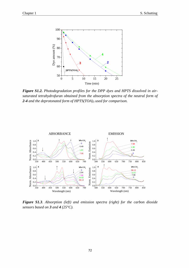
Chapter 1 S. Schutting
72
0 5 10 15 20 2550
60
70
80
90
100
4
2
Dye
am
oun
t (%
)
Time (min)
HPTS(TOA)3
3
Figure S1.2. Photodegradation profiles for the DPP dyes and HPTS dissolved in air-saturated tetrahydrofuran obtained from the absorption spectra of the neutral form of 2-4 and the deprotonated form of HPTS(TOA)3 used for comparison.
350 400 450 500 550 600 650 7000.0
0.2
0.4
0.6
0.8
1.0
500 550 600 650 700 750 800 8500.0
0.2
0.4
0.6
0.8
1.0
350 400 450 500 550 600 650 7000.0
0.2
0.4
0.6
0.8
1.0
500 550 600 650 700 750 800 8500.0
0.2
0.4
0.6
0.8
1.0
98.13
No
rm. A
bso
rban
ce 4 kPa CO2
2.940
7.0814.62
kPa CO2
07.0814.6298.13
No
rm.
Em
issi
on 4
Wavelength (nm)
No
rm.
Ab
sorb
an
ce 30
0.49
1.96
7.08
kPa CO2
Wavelength (nm)
EMISSION
Nor
m.
Em
issi
on 3 kPa CO
2
0
0.49
1.96
7.08
ABSORBANCE
Figure S1.3. Absorption (left) and emission spectra (right) for the carbon dioxide sensors based on 3 and 4 (25°C).
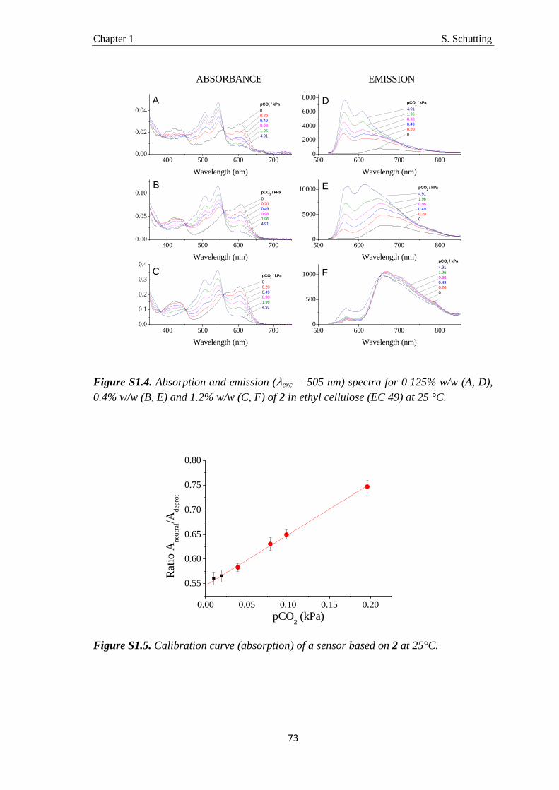
Chapter 1 S. Schutting
73
400 500 600 7000.00
0.02
0.04
500 600 700 8000
2000
4000
6000
8000
400 500 600 7000.00
0.05
0.10
500 600 700 8000
5000
10000
400 500 600 7000.0
0.1
0.2
0.3
0.4
500 600 700 8000
500
1000
Wavelength (nm)
A pCO2 / kPa
00.200.490.981.964.91
pCO2 / kPa
4.911.960.980.490.200
Wavelength (nm)
D
Wavelength (nm)
BpCO
2 / kPa
00.200.490.981.964.91
pCO2 / kPa
4.911.960.980.490.200
pCO2 / kPa
4.911.960.980.490.200
Wavelength (nm)
E
Wavelength (nm)
ABSORBANCE EMISSION
CpCO2 / kPa
00.200.490.981.964.91
Wavelength (nm)
F
Figure S1.4. Absorption and emission (λexc = 505 nm) spectra for 0.125% w/w (A, D), 0.4% w/w (B, E) and 1.2% w/w (C, F) of 2 in ethyl cellulose (EC 49) at 25 °C.
0.00 0.05 0.10 0.15 0.20
0.55
0.60
0.65
0.70
0.75
0.80
Ratio
An
eutr
al/A
depr
ot
pCO2 (kPa)
Figure S1.5. Calibration curve (absorption) of a sensor based on 2 at 25°C.

Chapter 1 S. Schutting
74
0 2 4
0.5
1.0
1.5
Ra
tio A
neut
ral/A
depr
ot
pCO2 (kPa)
Figure S1.6. Calibration curve (absorption) of a sensor based on 4 at 25°C. Calculated LOD 0.07 kPa.
0 1 2 3 4 5
0.0
0.2
0.4
0.6
0.8
1.0
Nor
m. F
luore
scen
ce In
tens
ity
at 5
65 n
m
pCO2 (kPa)
Figure S1.7. Temperature dependence for the CO2 sensor containing dye 2 in EC49 with TOAOH as base calibrated at 25 °C (red circles) and at 5°C (black squares).
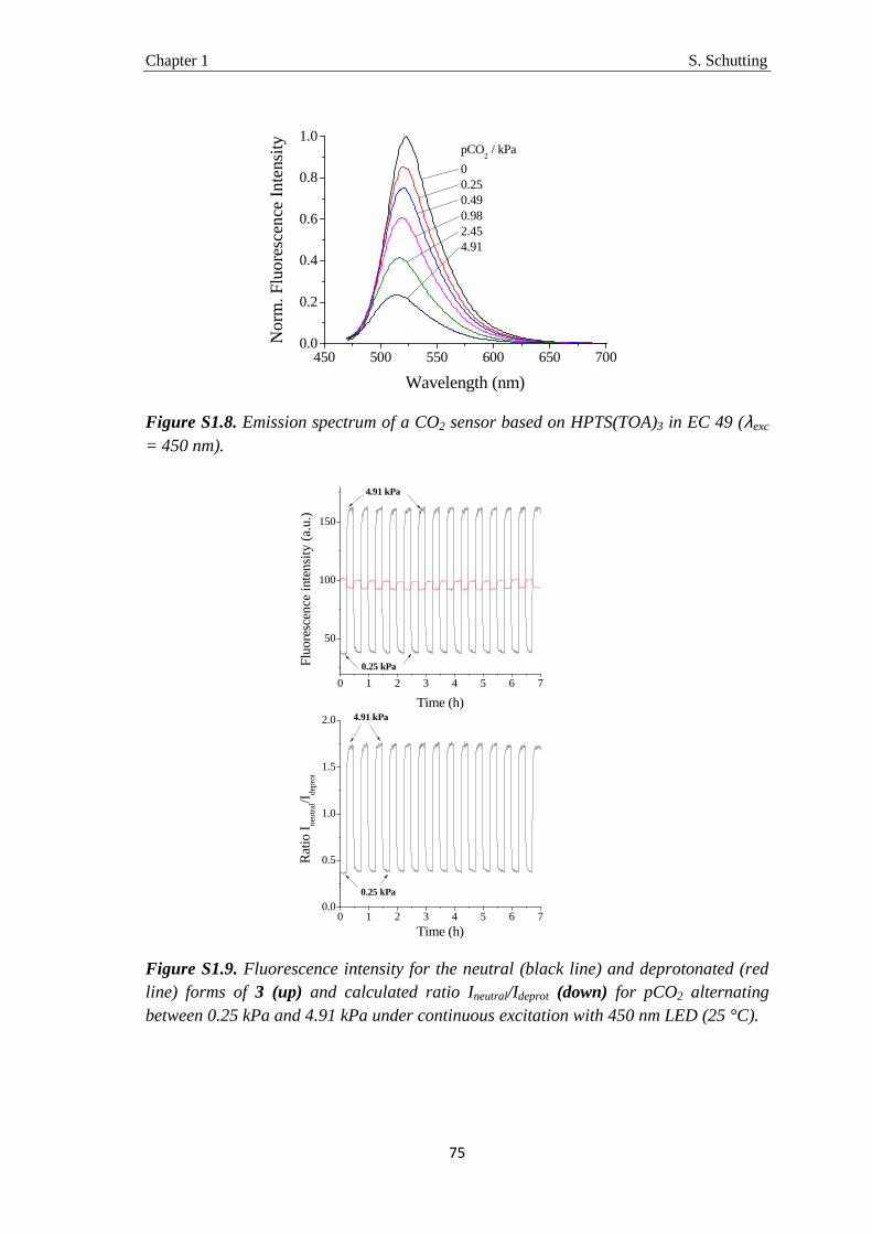
Chapter 1 S. Schutting
75
450 500 550 600 650 7000.0
0.2
0.4
0.6
0.8
1.0
No
rm.
Flu
ore
scen
ce In
tens
ity
Wavelength (nm)
pCO2 / kPa
00.250.490.982.454.91
Figure S1.8. Emission spectrum of a CO2 sensor based on HPTS(TOA)3 in EC 49 (λexc = 450 nm).
0 1 2 3 4 5 6 7
50
100
150
0 1 2 3 4 5 6 70.0
0.5
1.0
1.5
2.0
Flu
ores
cen
ce in
ten
sity
(a.
u.)
Time (h)
0.25 kPa
4.91 kPa
Rat
io I n
eutr
al/I
dep
rot
Time (h)
0.25 kPa
4.91 kPa
Figure S1.9. Fluorescence intensity for the neutral (black line) and deprotonated (red line) forms of 3 (up) and calculated ratio Ineutral/Ideprot (down) for pCO2 alternating between 0.25 kPa and 4.91 kPa under continuous excitation with 450 nm LED (25 °C).
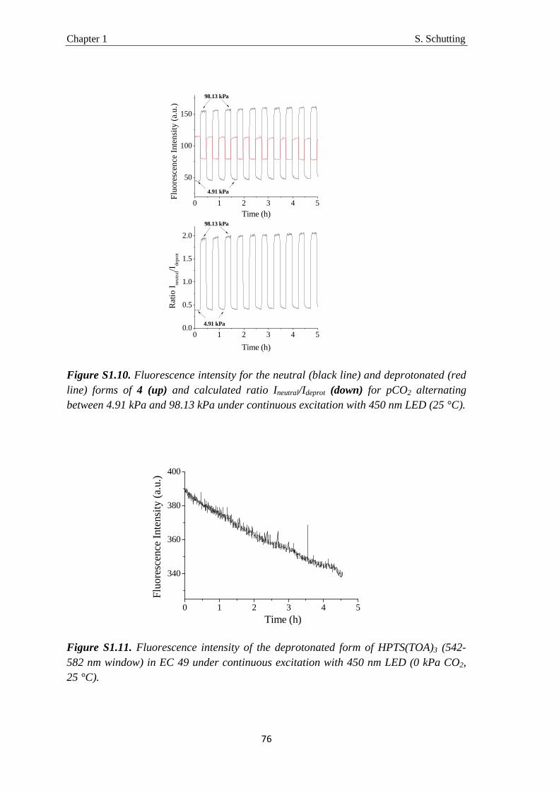
Chapter 1 S. Schutting
76
0 1 2 3 4 5
50
100
150
0 1 2 3 4 50.0
0.5
1.0
1.5
2.0
Flu
ore
scen
ce I
nten
sity
(a.
u.)
Time (h)
Rat
io I n
eutr
al/I de
pro
t
Time (h)
98.13 kPa
4.91 kPa
98.13 kPa
4.91 kPa
Figure S1.10. Fluorescence intensity for the neutral (black line) and deprotonated (red line) forms of 4 (up) and calculated ratio Ineutral/Ideprot (down) for pCO2 alternating between 4.91 kPa and 98.13 kPa under continuous excitation with 450 nm LED (25 °C).
0 1 2 3 4 5
340
360
380
400
Flu
ores
cen
ce In
tens
ity (
a.u
.)
Time (h)
Figure S1.11. Fluorescence intensity of the deprotonated form of HPTS(TOA)3 (542-582 nm window) in EC 49 under continuous excitation with 450 nm LED (0 kPa CO2, 25 °C).

Chapter 1 S. Schutting
77
Figure S1.12. 1H NMR spectrum of 1 (300 MHz, DMSO-d6).
Figure S1.13. 1H 1H COSY NMR spectrum of 1 (DMSO-d6).

Chapter 1 S. Schutting
78
m/z560 580 600 620 640 660 680 700 720 740 760 780 800 820 840 860 880
%
0
100
20121122_Schutting_alpha 66 (1.100) Sb (99,20.00 ); Cm ((40:46+66:71+75:81+84:89)) TOF LD+ 4.63e3677.0
676.0
714.9
678.0
679.0
680.0
715.9
716.9
717.9
Figure S1.14. MALDI-TOF mass spectrum of 1.
m/z620 630 640 650 660 670 680 690 700 710 720 730 740 750 760 770 780
%
0
100
%
0
100
%
0
100
20121122_Schutting_alpha (0.017) Is (0.05,0.01) C30H18K2N2O8S2K TOF LD+ 5.10e12714.9416
716.9407
717.9430
20121122_Schutting_alpha (0.017) Is (0.05,0.01) C30H18K2N2O8S2H TOF LD+ 5.47e12676.9857
677.9888
20121122_Schutting_alpha 66 (1.100) Sb (99,20.00 ); Cm ((40:46+66:71+75:81+84:89)) TOF LD+ 4.63e3676.9900
675.9839
714.9446
677.9902
678.9905
679.9918
715.9470
717.9454
Experimental
Theoretical isotope pattern [MH]+
Theoretical isotope pattern [MK]+
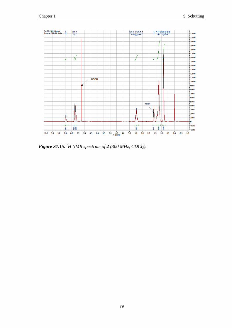
Chapter 1 S. Schutting
79
Figure S1.15. 1H NMR spectrum of 2 (300 MHz, CDCl3).
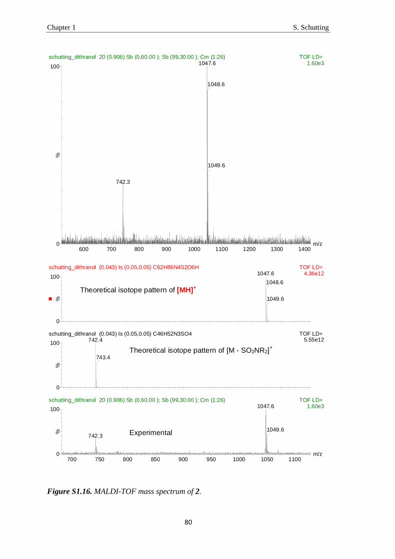
Chapter 1 S. Schutting
80
Figure S1.16. MALDI-TOF mass spectrum of 2.
m/z700 750 800 850 900 950 1000 1050 1100
%
0
100
%
0
100
%
0
100
schutting_dithranol (0.043) Is (0.05,0.05) C62H86N4S2O6H TOF LD+ 4.36e121047.6
1048.6
1049.6
schutting_dithranol (0.043) Is (0.05,0.05) C46H52N3SO4 TOF LD+ 5.55e12742.4
743.4
schutting_dithranol 20 (0.906) Sb (0,60.00 ); Sb (99,30.00 ); Cm (1:26) TOF LD+ 1.60e31047.6
742.31049.6
m/z600 700 800 900 1000 1100 1200 1300 1400
%
0
100
schutting_dithranol 20 (0.906) Sb (0,60.00 ); Sb (99,30.00 ); Cm (1:26) TOF LD+ 1.60e31047.6
742.3
1048.6
1049.6
Experimental
Theoretical isotope pattern of [MH]+
Theoretical isotope pattern of [M - SO2NR2]+

Chapter 1 S. Schutting
81
m/z480 500 520 540 560 580 600 620 640 660 680 700 720 740 760 780
%
0
100
mphdkppmonosa 2 (0.097) Cn (Cen,1, 20.00, Ht); Sb (99,10.00 ); Cm (1:39) TOF LD+ 1.67e4592.3
591.3 593.3
594.3
614.3
Figure S1.17. 1H NMR spectrum of 3 (300 MHz, DMSO-d6).

Chapter 1 S. Schutting
82
Figure S1.18. MALDI-TOF mass spectrum of 3.
Figure S1.19. 1H NMR spectrum of 4 (300 MHz, CDCl3).
m/z550 560 570 580 590 600 610 620 630 640
%
0
100
%
0
100
mphdkppmonosa (0.048) Is (0.05,0.05) C34H45N3O4SH TOF LD+ 6.35e12592.3209
593.3240
mphdkppmonosa 2 (0.097) Cn (Cen,1, 20.00, Ht); Sb (99,10.00 ); Cm (1:39) TOF LD+ 1.67e4592.3214
Experimental

Chapter 1 S. Schutting
83
Figure S1.20. MALDI-TOF mass spectrum of 4.
m/z830 840 850 860 870 880 890 900 910 920 930 940 950 960 970
%
0
100
%
0
100
mphdkppdisa (0.048) Is (0.05,0.05) C50H78N4O6S2H TOF LD+ 4.99e12895.5441
896.5472
mphdkppdisa 40 (1.933) Cn (Cen,1, 70.00, Ht); Sb (99,10.00 ); Cm (1:43) TOF LD+ 1.35e4895.5469
896.5515
m/z600 700 800 900 1000 1100 1200 1300
%
0
100
mphdkppdisa 40 (1.933) Cn (Cen,1, 70.00, Ht); Sb (99,10.00 ); Cm (1:43) TOF LD+ 1.35e4895.5
894.5779.4591.3
896.6
897.6
898.6
899.5
Experimental
Theoretical isotope pattern of [MH]+
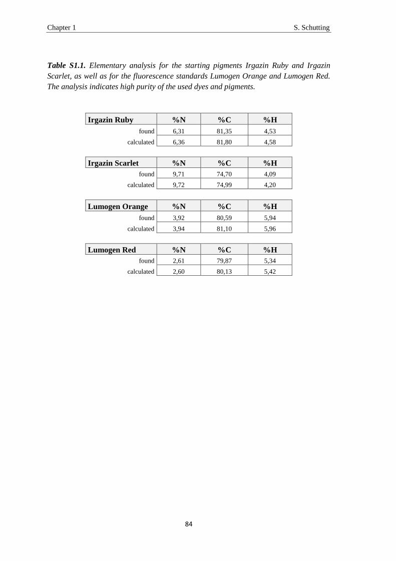
Chapter 1 S. Schutting
84
Table S1.1. Elementary analysis for the starting pigments Irgazin Ruby and Irgazin Scarlet, as well as for the fluorescence standards Lumogen Orange and Lumogen Red. The analysis indicates high purity of the used dyes and pigments.
Irgazin Ruby %N %C %H found 6,31 81,35 4,53
calculated 6,36 81,80 4,58
Irgazin Scarlet %N %C %H found 9,71 74,70 4,09
calculated 9,72 74,99 4,20
Lumogen Orange %N %C %H found 3,92 80,59 5,94
calculated 3,94 81,10 5,96
Lumogen Red %N %C %H found 2,61 79,87 5,34
calculated 2,60 80,13 5,42
Chapter 2 S. Schutting
85
Chapter 2
Scope of this chapter
In the previous chapter a new indicator class based on diketo-pyrrolo-pyrroles was
presented. It was shown, that this class is a promising alternative to known state-of-the-
art indicators, such as HPTS. It was also shown, that there are still demands to meet,
such as high quantum yields for the deprotonated indicator forms or even higher
sensitivity.
In chapter 2, an enhancement of this indicator class will be presented. The pKa value of
the new indicator was even more increased due to substitution with electron-donating
groups. Thus, the presented carbon dioxide sensors featured extremely high sensitivity.
Furthermore, the spectral properties were tuned to match the color channels of a
commercially available red/green/blue (RGB) camera enabling read-out via imaging.
Additionally, the quantum yields for both, the protonated and the deprotonated form, are
very high.

Chapter 2 S. Schutting
86
Chapter 2 S. Schutting
87
New Highly Fluorescent pH Indicator for Ratiometric RGB Imaging of pCO2
This chapter was published in Methods and Applications in Fluorescence, 2014, 2, 1- 8; doi: 10.1088/2050-6120/2/2/024001
Authors: Susanne Schutting, Ingo Klimant, Dirk de Beer and Sergey M. Borisov
A new diketo-pyrrolo-pyrrole (DPP) indicator dye for optical sensing of carbon dioxide
is prepared via a simple 1 step synthesis from commercially available low cost
“Pigment Orange 73”. The pigment is modified via alkylation of one of the lactam
nitrogens with a tert-butylbenzyl group. The indicator dye is highly soluble in organic
solvents and in polymers and shows pH-dependent absorption (λmax 501 and 572 nm
for the protonated and deprotonated form, respectively) and emission spectra (λmax
524 and 605 nm for the protonated and deprotonated form, respectively). Both the
protonated and the deprotonated form show high fluorescence quantum yields (Φprot
0.86; Φdeprot 0.66). Hence, colorimetric read-out and ratiometric fluorescence
intensity measurements are possible. The emission of the two forms of the indicator
excellently matches the response of the green and the red channel of an RGB camera.
This enables imaging of carbon dioxide distribution with simple and low cost optical
set-up. The sensor based on the new DPP dye shows very high sensitivity and is
particularly promising for monitoring of atmospheric levels of carbon dioxide.
Introduction
Carbon dioxide is one of the most important parameters for environmental monitoring,
marine research and oceanography. The increase of carbon dioxide concentration in the
oceans causes acidification, which severely affects the flora and fauna therein.9,14,96–
98,138 The analytical tools for detection of dissolved carbon dioxide are limited to only a
few such as the Severinghaus electrode77 or IR analyzers. The former suffers from
electromagnetic interferences and has slow response. IR analyzers are fast,61 but are

Chapter 2 S. Schutting
88
mostly suitable for measurements in gaseous phase85,86 since water causes a significant
interference. Several new concepts of carbon dioxide chemosensors were published in
recent years;116–118,139,140 however so called ‘plastic type’ sensors remain the most
common ones.51,89 These materials contain a pH-sensitive dye and a base (most
commonly a quaternary ammonium base) dissolved in a polymer matrix. The pH
indicator responds to the analyte by altering its optical properties, mostly the absorption
or emission characteristics. In case of the fluorescent sensors referencing of the
fluorescence intensity is required to enable reliable measurements. This can be achieved
by adding a second analyte-insensitive dye which emission spectrum is clearly
separated from that of the indicator (ratiometric read-out) or which luminescence decay
time is significantly different from the lifetime of the indicator (dual lifetime
referencing scheme).141–143 In both schemes photobleaching (indicator, reference dye or
both) causes a dramatic change of the emission ratio of the indicator and the reference
dye. Therefore, self-referencing indicator dyes are highly desirable; however only a few
such dyes have been reported.144–147 Spectral compatibility with commercially available
red/green/blue (RGB) cameras is also of great interest. The read-out with RGB cameras
is a simple and low cost technique for imaging different parameters such as CO2,148
pH149–152 or oxygen,153–156 to name only a few. Recently, we presented a new class of
pH-sensitive indicator dyes based on diketo-pyrrolo-pyrroles (DPPs).152,157 DPPs are
usually insoluble in organic solvents and are mainly used as pigments.119 The soluble
derivatives (mainly N-alkylated dyes)120,158–164 are also of much practical interest and
are applied e.g. in photovoltaics.158–160 So far only a few applications of DPPs as
fluorescent probes are found in the literature.127,128,152,165 The new DPP-based pH
indicators were shown to be highly promising for application in optical pH and carbon
dioxide sensors.152,157 Particularly, dual emission from the protonated and deprotonated
forms enabled ratiometric read-out, but the emission from the deprotonated form was
much weaker than that of the protonated form (Φprot ≈ 1 and Φdeprot ≈ 0.1).
Unfortunately, these dually emitting dyes were not fully compatible with the green and
red channels of the digital cameras.166 In this study, we present a new DPP-based pH
indicator which overcomes these drawbacks. It will be shown that the new dye
possesses high fluorescence quantum yields for both the protonated and the
deprotonated form and is excellently suitable for the RGB read-out. The CO2 sensor
shows very high sensitivity and is particularly useful for monitoring atmospheric levels
of the analyte.
Chapter 2 S. Schutting
89
Experimental Details
Materials
1,4-diketo-3,6-bis(4-tert-butyl-phenyl)-2,5-dihydro pyrrolo[3,4-c]pyrrole (Pigment
Orange 73), 1,6,7,12-tetraphenoxy-N,N´-bis(2,6-diisopropylphenyl)-perylene-3,4:9,10-
tertracarboxylic bisimide (Lumogen-Red) and N,N´-bis(2,6-diisopropylphenyl)-
perylene-3,4:9,10-tertracarboxylic bisimide (Lumogen-Orange) were purchased from
Kremer Pigments (Germany, www.kremer-pigmente.com). Ethyl cellulose 49 (EC49,
ethoxyl content 49%), sodium sulfate (anhydrous), sodium tert-butoxide, 4-tert-
butylbenzyl bromide, tetraoctylammonium hydroxide solution (TOAOH, 20% in
methanol) and anhydrous dimethylformamide were obtained from Sigma-Aldrich
(www.sigmaaldrich.com). All other solvents were purchased from VWR (Austria,
www.vwr.com). The silicone components: vinyl terminated polydimethylsiloxane
(viscosity 1000 cSt.), (25-35% methylhydrosiloxane)-dimethylsiloxane copolymer
(viscosity 25-35 cSt.), 1,3,5,7-tetravinyl-1,3,5,7-tetramethylcyclotetrasiloxane and the
platinum-divinyltetramethyldisiloxane complex were received from ABCR (Germany,
www.abcr.de). Ultrafine hydrophobic titanium dioxide P170 was purchased from
Kemira (www.kemira.com). High purity nitrogen, 5% carbon dioxide in nitrogen, 0.2%
carbon dioxide in nitrogen and carbon dioxide were obtained from Air Liquide (Austria,
www.airliquide.at). Poly(ethylene terephthalate) (PET) support Melinex 505 was
obtained from Pütz (Germany, www.puetz-folien.com). Silica-gel was received from
Roth (www.carlroth.com). Synthesis of BiPh-DiSA (3,6-bis[4´-bis(2-
ethylhexyl)sulfonylamide-1,1´-biphenyl-4-yl]-2,5-dihydropyrrolo[3,4-c]pyrrole-1,4-
dione) and MoPh-DiSA (3,6-bis[4-bis(2-ethylhexyl)sulfonylamide-phenyl]-2,5-
dihydropyrrolo[3,4-c]pyrrole-1,4-dione) was described before.157
Synthesis of 2-hydro-5-tert-butylbenzyl-3,6-bis(4-tert-butyl-phenyl)-pyrrolo[3,4-
c]pyrrole-1,4-dione (DPPtBu3)
Pigment Orange 73 (2 g, 4.9 mmol) and sodium tert-butoxide (0.96 g, 10 mmol) were
dissolved in anhydrous dimethylformamide (80 ml). 4-tert-butylbenzyl bromide (1.1 ml,
6.0 mmol) was added dropwise. After stirring for 8 h at 60 °C the mixture was diluted
with deionized water. The dye was extracted with dichloromethane and hydrochloric
acid and sodium chloride were added to facilitate the phase separation. The organic

Chapter 2 S. Schutting
90
phase was collected, dried over anhydrous sodium sulfate and evaporated to dryness
under reduced pressure. The crude product was purified via column chromatography on
silica gel using dichloromethane/tetrahydrofuran (98:2). The product was dissolved in
dichloromethane and precipitated with hexane to give an orange powder (0.23 g, 8.3%
of theoretical yield of DPPtBu3). DI-EI-TOF: m/z of [MH]+ found 546.3259, calculated
546.3246. 1H NMR (300MHz, CDCl3) δ 9.38 (s, 1H), 8.28 (d, 2H), 7.77 (d, 2H), 7.53
(d, 2H), 7.50 (d, 2H), 7.34 (d, 2H), 7.16 (d, 2H), 5.04 (s, 2H), 1.35 (s, 18H), 1.30 (s,
9H). Analysis for C37H42N2O2 found: C81.12, H7.59, N5.12, calculated: C81.28, H7.74,
N5.12.
Preparation of the Planar Optodes
“Cocktail 1” containing X mg of the dye and 100 µl the tetraoctylammonium hydroxide
solution (20% TOAOH in methanol) was purged with carbon dioxide gas. X was 3.0
mg and 0.5 mg for the absorption and emission measurements, respectively. “Cocktail
2” containing 200 mg ethyl cellulose (EC49) dissolved in 3800 mg of a toluene:ethanol
mixture (6:4 w/w) was added to the “cocktail 1”. The resulting solution was knife-
coated on a dust-free PET or glass support. A sensing film of ~7.5 µm thickness was
obtained after evaporation of the solvent. The sensing film was covered with a gas-
permeable ~22 µm-thick silicone layer by knife-coating “cocktail 3” consisting of 800
mg vinyl terminated polydimethylsiloxane, 32 µl (25-35% methylhydrosiloxane)-
dimethylsiloxane copolymer, 2 µl 1,3,5,7-tetravinyl-1,3,5,7-
tetramethylcyclotetrasiloxane and 4 µl platinum-divinyltetramethyldisiloxane complex
dissolved in 1600 mg hexane. For emission measurements a similar layer was prepared
but 200 mg of titanium dioxide were dispersed in “cocktail 3”. The sensors were kept in
an oven (60 °C) for 10-15 min to complete polymerization of the silicone rubber.
Methods 1H NMR spectra were recorded on a 300 MHz instrument (Bruker) in CDCl3 with TMS
as standard. Absorption spectra were recorded on a Cary 50 UV-Vis spectrophotometer
(www.varianinc.com). Determination of the molar absorption coefficients was carried
out as an average of 3 independent measurements. Photobleaching experiments were
performed by irradiating the samples (2.5 ml) with the light of a high-power 10 W LED
array (λmax 458 nm, 3 LEDs, www.led-tech.de) operated at 6 W input power. A lens

Chapter 2 S. Schutting
91
(Edmund optics, www.edmundoptics.de) was used to focus the light of the LED array
on the glass cuvette (photon flux: ∼4000 µmol⋅s-1⋅m-2 as determined with a Li-250A
light meter from Li-COR, www.licor.com). The photodegradation profiles were
obtained by monitoring the absorption spectra of the respective dye dissolved in
tetrahydrofuran and represented an average from three independent experiments. The
solutions were homogenized by shaking after each illumination period. Fluorescence
spectra were recorded on a Hitachi F-7000 fluorescence spectrometer
(www.hitachi.com) equipped with a red-sensitive photomultiplier R928 from
Hamamatsu (www.hamamatsu.com). Relative fluorescence quantum yields were
determined according to Demas and Crosby.129 The solutions of Lumogen-Orange (Φ ≈
1) and Lumogen-Red (Φ ≈ 0.96)130,131 in chloroform were used as standards for the
protonated and the deprotonated form, respectively. Three independent measurements
were performed for determination of the relative quantum yields and the average value
obtained was used. In case of the sensing materials only the absolute quantum yields
were determined. These measurements were performed on a Fluorolog3 fluorescence
spectrometer (www.horiba.com) equipped with a NIR-sensitive photomultiplier R2658
from Hamamatsu (300-1050 nm) and an integrating sphere (Horiba).
Gas calibration mixtures were obtained using a gas mixing device from MKS
(www.mksinst.com). The gas mixture was humidified to about 85% relative humidity
(saturated KCl solution) prior entering the calibration chamber. Temperature was
controlled by a cryostat ThermoHaake DC50. Photographic images were acquired with
a Canon 5D camera equipped with a Canon 24-105L objective and two layers of a LEE
plastic filter “spring yellow”. The same high-power 10 W LED array (λmax 458 nm, 3
LEDs, www.led-tech.de) as for the photodegradation experiments combined with a
short-pass BG-12 filter served as an excitation source.
Results and Discussion
Synthesis
The DPP chromophores possess planar structure and are poorly soluble in organic
solvents.133 Low solubility prevents the dyes from application as indicators in optical
sensors. We previously demonstrated that the dyes are pH-sensitive due to the

Chapter 2 S. Schutting
92
deprotonation of the lactam nitrogen.152,157 Modification of the phenyl rings with bulky
substituents rendered the pigments soluble in organic solvents and polymers and the pH
sensitivity was preserved. On the other hand, alkylation of both lactam nitrogens is
another simple way to greatly enhance the solubility of DPPs.134 Evidently such
modification renders the DPPs pH-insensitive. Mono-N-alkylation of the commercially
available Pigment Orange 73 (scheme 2.1) with a tert-butylbenzyl-group preserves pH
sensitivity and dramatically improves the solubility of the dye in such common solvents
as toluene, tetrahydrofuran (THF), dichloromethane, chloroform, etc. Thus, the dye
becomes suitable for application in optical plastic carbon dioxide sensors.
Scheme 2.1. Synthesis of DPPtBu3 starting from Pigment Orange 73.
Photophysical Properties
Absorption and emission spectra for DPPtBu3 dissolved in THF are shown in figure 2.1.
The protonated form of the dye absorbs in the blue and emits in the green part of the
electromagnetic spectrum. Absorption and emission spectra for the deprotonated form
are bathochromically shifted by ~70 nm compared to the protonated form. This is about
50 nm less than in case of previously reported DPP dye MoPh-DiSA (3,6-bis[4-bis(2-
ethylhexyl)sulfonylamide-phenyl]-2,5-dihydropyrrolo[3,4-c]pyrrole-1,4-dione, table
2.1).157 The mono-alkylated dye shows spectral maxima at shorter wavelengths than not
alkylated MoPh-DiSA. The molar absorption coefficients are typical for the DPP dyes
(table 2.1). The fluorescence quantum yields are rather high and are comparable for
both forms of DPPtBu3 (table 2.1). On the contrary, the emission of the deprotonated
form of MoPh-DiSA is much weaker than the emission of the protonated form.

Chapter 2 S. Schutting
93
400 500 600 700 8000.0
0.2
0.4
0.6
0.8
1.0
400 500 600 700 8000.0
0.2
0.4
0.6
0.8
1.0N
orm
. A
bsor
banc
e&
Flu
ores
cen
ce I
nte
nsity
Wavelength (nm)
N
NH
O
O
protonated Ind
A
B
N
N-
O
O
Nor
m.
Abs
orba
nce
& F
luor
esc
ence
Inte
nsity
Wavelength (nm)
deprotonated Ind-
Figure 2.1. Absorption (solid lines) and emission (λexc 430nm, dashed lines) spectra of the protonated form (A) and the deprotonated form (B) of DPPtBu3 in THF.
Table 2.1. Comparison of the photophysical properties of DPPtBu3 and the DPP dye MoPh-DiSA in tetrahydrofuran (THF) at 25 °C.
Protonated form Deprotonated form
Dye λabs (ε·10-3)
[nm (M -1cm-1)]
λem
[nm]
ΦΦΦΦ
λabs (ε·10-3)
[nm (M -1cm-1)]
λem
[nm]
ΦΦΦΦ
DPPtBu3 472(25.2); 501(26.8) 524 0.86 572(17.6) 605 0.66
MoPh-DiSA 491(29.8); 528(36.9) 543;583 1 655(23.0) 708 0.11
DPPtBu3 is highly soluble in organic solvents, but is not soluble in water. Therefore,
determination of the pKa in aqueous buffers is not possible. The pKa value in a mixture
of tetrahydrofuran and aqueous buffer (1:1 v/v) was estimated to be rather high (~12.7;
supporting information, figure S2.1). It should be noted that this is very rough
estimation because of the high content of organic solvent and the alkali error of the pH
electrode at high pH. The pKa value for DPPtBu3 is likely to be higher than that for the
recently presented DPP dye (3,6-bis[4´(3´)-disulfo-1,1´-biphenyl-4-yl]-2,5-

Chapter 2 S. Schutting
94
dihydropyrrolo[3,4-c]pyrrole-1,4-dione dipotassium salt)157 which showed a pKa of
~11.8 since electron-donating tert-butyl groups of DPPtBu3 are expected to elevate the
dissociation constant.
Carbon Dioxide Sensors
DPPtBu3 and the base tetraoctylammonium hydroxide (TOAOH) were non-covalently
entrapped in an ethyl cellulose (EC49) matrix to obtain plastic type carbon dioxide
sensors. The response of the sensor can be described by the following equation:
Ind-TOA+ + CO2 + H2O ↔ IndH + TOA+HCO3-
It is essential that the carbon dioxide sensors are kept humid during the measurements
to enable reversible and reliable response (supporting information, figure S2.3). The
sensors respond to increasing pCO2 with a color change from pink in the absence of
CO2 to yellow in the presence of CO2. This corresponds to the change in the absorption
spectra of the sensing material (figure 2.2A). Isosbestic points (IP) at 430 nm and 522
nm are clearly visible which indicates that only two forms of the dye are present in the
acid-base equilibrium. The sensor shows red fluorescence at low pCO2 and green
fluorescence at high pCO2 (figure 2.2B). For emission measurements commercially
available intense LEDs emitting at wavelengths between 430 nm and 470 nm are
suitable as excitation sources. As can be seen, the emission intensity of the deprotonated
form decreases, whereas the intensity of the protonated form increases with increasing
pCO2 (figure 2.2C). Importantly, virtually no fluorescence of the protonated form (λmax
529 nm) is detectable in the absence of carbon dioxide, so that the relative signal
changes are very high at low pCO2. Comparison of the absorption and emission spectra
(figure 2.2A and 2.2B) indicates the effect of Förster resonance energy transfer (FRET)
from the protonated form of the indicator to its deprotonated form. Indeed, the emission
spectrum of the former and the absorption spectrum of the latter show almost perfect
overlap (figure 2.1). The dye concentration dramatically affects the emission due to
FRET (supporting information, figure S2.4). For example, in case of high dye
concentration (1.5% w/w) the emission spectrum is dominated by the deprotonated form
at pCO2 below 5 kPa. Hence, the dynamic range of the sensing materials relying on
fluorescence intensity read-out can be tuned by adjusting the concentration of the

Chapter 2 S. Schutting
95
indicator dye. Highly sensitive fluorescent sensors are obtained only for relatively low
dye concentrations.
400 500 600 7000.0
0.2
0.4
0.6
0.8
1.0
500 600 700 8000.0
0.2
0.4
0.6
0.8
1.0
0.0 2.5 5.0 7.5 10.0
0.0
0.2
0.4
0.6
0.8
C
B
Abs
orba
nce
Wavelength (nm)
0 kPa CO2
0.2 kPa CO2
0.5 kPa CO2
1.0 kPa CO2
2.5 kPa CO2
98.1 kPa CO2
AF
luor
esce
nce
Inte
nsity
(a.
u.)
Wavelength (nm)
GREENRED 98.1 kPa CO
2
7.1 kPa CO2
2.5 kPa CO2
1.0 kPa CO2
0.25 kPa CO2
0 kPa CO2
Flu
ores
cenc
e In
tens
ity
at 5
29
nm
& 6
30 n
m (
a.u.
)
pCO2 (kPa)
!
Figure 2.2. Absorption (A) and emission (B) spectra (λexc 430 nm) of the CO2 sensor based on DPPtBu3 in ethyl cellulose 49 and TOAOH as base including the spectral sensitivity for the green and the red detection channels of the RGB camera (green and red dotted lines, B). (C) the fluorescence intensity changes for the protonated form (at 529 nm, black curve) and the deprotonated form (at 630 nm, blue curve) with increasing pCO2, the fit is performed according to the exponential growth/decay model, respectively; high relative signal changes at low pCO2 values (red box and exclamation mark) are indicated.

Chapter 2 S. Schutting
96
Compared to the solution the spectral properties of the indicator are mostly preserved
(figure 2.1 and figure 2.2). The fluorescence quantum yields are high (Φ ≈ 1.0 and 0.63)
for the protonated form and the deprotonated form, respectively. Carbon dioxide sensors
based on DPPtBu3 are highly sensitive to pCO2 at 25°C (red box and exclamation mark
in figure 2.2C). Due to better solubility of CO2 at lower temperatures, the sensitivity is
even higher at 5°C (figure 2.3). It should be mentioned that rather strong temperature
dependence is common for the plastic type carbon dioxide sensors,61 but development
of the materials with lower temperature cross-talk was beyond the scope of this study.
Low levels of pCO2 need to be measured in a completely decarbonated system – from
gas lines, gas mixing device and humidifier to the flow-through cell – which is difficult
to achieve in practice. Particularly, precise calibration at the atmospheric level of 0.04
kPa pCO2 and lower is challenging. The exchange of PET foil to gas-impermeable glass
support improved the linearity at low pCO2, but did not solve the contamination
problem entirely. This is well observable in the absorption measurements where such
contamination results in larger deviation than during fluorescence measurements
influenced by FRET (figure 2.3B and 2.3D, respectively). Determination of the limit of
detection (LOD) was therefore not possible. Nevertheless, it can be concluded that the
sensor shows excellent response at atmospheric levels (pCO2 0.04 kPa ≈ 400 ppm in the
gas phase ≈ 11.6 µmol/L in water at 298.15 K) of carbon dioxide and therefore is highly
promising for e.g. oceanographic applications.
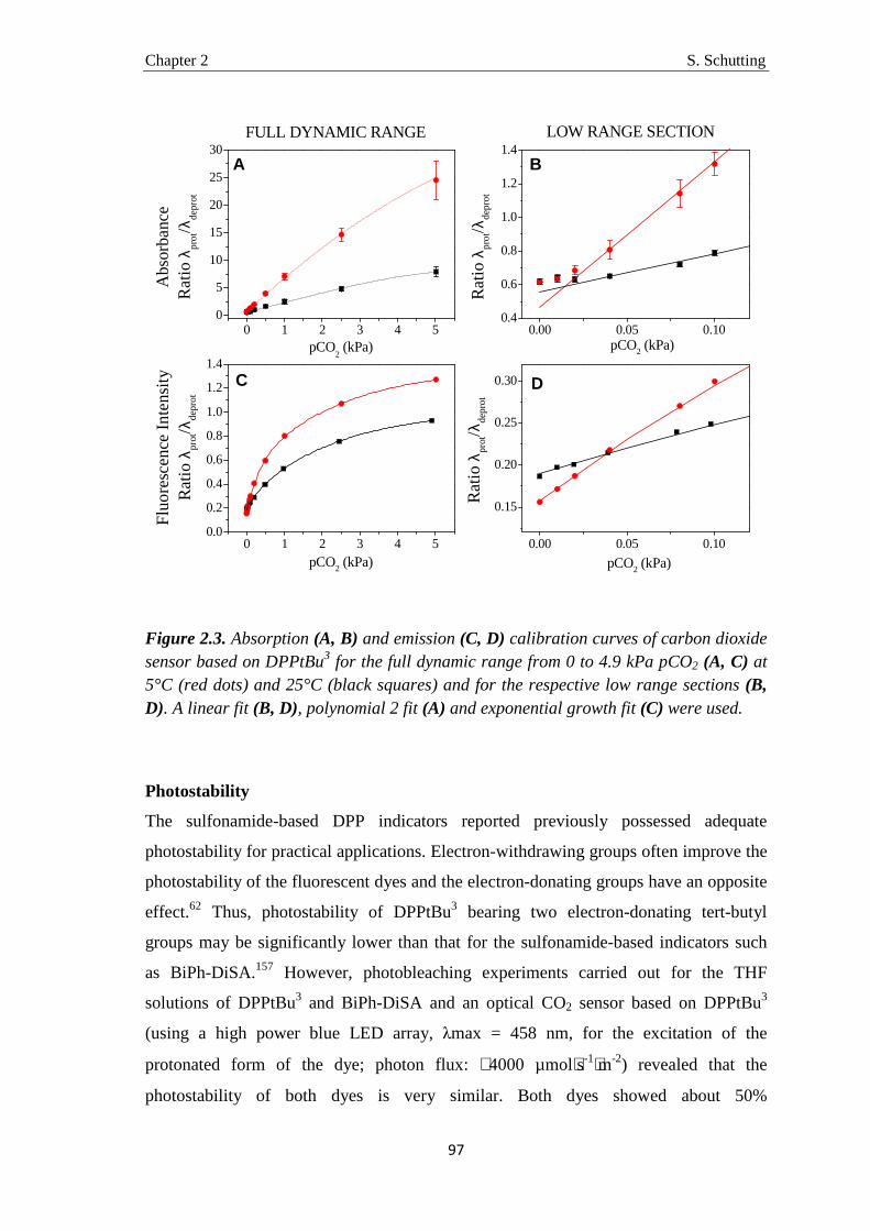
Chapter 2 S. Schutting
97
0 1 2 3 4 50.0
0.2
0.4
0.6
0.8
1.0
1.2
1.4
Flu
ore
sce
nce
Inte
nsity
Ra
tio λ pr
ot/λ
depr
ot
pCO2 (kPa)
A
0.00 0.05 0.10
0.15
0.20
0.25
0.30
B
Ra
tio λ pr
ot/λ
depr
ot
pCO2 (kPa)
0 1 2 3 4 50
5
10
15
20
25
30LOW RANGE SECTION
C
Abs
orba
nce
Ra
tio λ pr
ot/λ
depr
ot
pCO2 (kPa)
FULL DYNAMIC RANGE
0.00 0.05 0.100.4
0.6
0.8
1.0
1.2
1.4
D
Ra
tio λ pr
ot/λ
depr
ot
pCO2 (kPa)
Figure 2.3. Absorption (A, B) and emission (C, D) calibration curves of carbon dioxide sensor based on DPPtBu3 for the full dynamic range from 0 to 4.9 kPa pCO2 (A, C) at 5°C (red dots) and 25°C (black squares) and for the respective low range sections (B, D). A linear fit (B, D), polynomial 2 fit (A) and exponential growth fit (C) were used.
Photostability
The sulfonamide-based DPP indicators reported previously possessed adequate
photostability for practical applications. Electron-withdrawing groups often improve the
photostability of the fluorescent dyes and the electron-donating groups have an opposite
effect.62 Thus, photostability of DPPtBu3 bearing two electron-donating tert-butyl
groups may be significantly lower than that for the sulfonamide-based indicators such
as BiPh-DiSA.157 However, photobleaching experiments carried out for the THF
solutions of DPPtBu3 and BiPh-DiSA and an optical CO2 sensor based on DPPtBu3
(using a high power blue LED array, λmax = 458 nm, for the excitation of the
protonated form of the dye; photon flux: ∼4000 µmol⋅s-1⋅m-2) revealed that the
photostability of both dyes is very similar. Both dyes showed about 50%
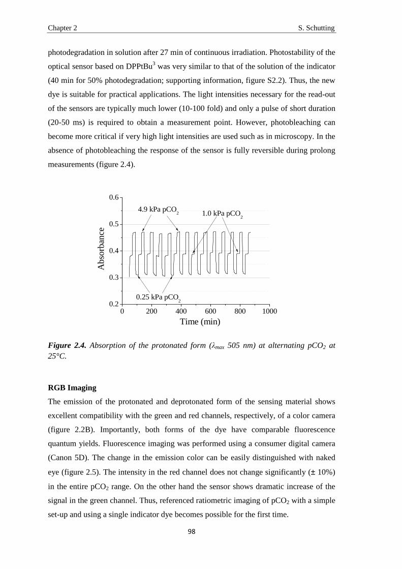
Chapter 2 S. Schutting
98
photodegradation in solution after 27 min of continuous irradiation. Photostability of the
optical sensor based on DPPtBu3 was very similar to that of the solution of the indicator
(40 min for 50% photodegradation; supporting information, figure S2.2). Thus, the new
dye is suitable for practical applications. The light intensities necessary for the read-out
of the sensors are typically much lower (10-100 fold) and only a pulse of short duration
(20-50 ms) is required to obtain a measurement point. However, photobleaching can
become more critical if very high light intensities are used such as in microscopy. In the
absence of photobleaching the response of the sensor is fully reversible during prolong
measurements (figure 2.4).
0 200 400 600 800 10000.2
0.3
0.4
0.5
0.6
1.0 kPa pCO2
4.9 kPa pCO2
Abso
rbance
Time (min)
0.25 kPa pCO2
Figure 2.4. Absorption of the protonated form (λmax 505 nm) at alternating pCO2 at 25°C.
RGB Imaging
The emission of the protonated and deprotonated form of the sensing material shows
excellent compatibility with the green and red channels, respectively, of a color camera
(figure 2.2B). Importantly, both forms of the dye have comparable fluorescence
quantum yields. Fluorescence imaging was performed using a consumer digital camera
(Canon 5D). The change in the emission color can be easily distinguished with naked
eye (figure 2.5). The intensity in the red channel does not change significantly (± 10%)
in the entire pCO2 range. On the other hand the sensor shows dramatic increase of the
signal in the green channel. Thus, referenced ratiometric imaging of pCO2 with a simple
set-up and using a single indicator dye becomes possible for the first time.

Chapter 2 S. Schutting
99
Figure 2.5. Photographic images of the planar optode based on DPPtBu3 under illumination with a 458-nm LED array acquired with a Canon 5D digital camera equipped with a long-pass “spring yellow” filter (Leefilters) (A) and the respective calibration plot for the ratio of fluorescence intensities for the red and green channel (B). The insert shows the curve for low pCO2 range.
Conclusions
A new pH-sensitive indicator dye based on a diketo-pyrrolo-pyrrole chromophore is
presented. A low cost starting pigment was chemically modified in one step via N-
alkylation. The resulting dye is well soluble in organic solvents and polymers and is
highly promising for preparation of carbon dioxide sensors. The features include high
fluorescence quantum yields for the protonated and the deprotonated form of the dye
and excellent compatibility of both emissions with the green and red channels of an
RGB camera. These properties enable self-referenced ratiometric imaging of pCO2 with
a single indicator. The optode shows excellent sensitivity at atmospheric levels of
carbon dioxide. This makes the sensor a promising analytical tool for application in
environmental monitoring, marine research and oceanography, for example for
monitoring of ocean acidification.
Acknowledgments
This work was supported by 7th framework EU project ECO2. We thank Robert Saf
(Institute for Chemistry and Technology of Materials, Graz University of Technology,
Austria) for mass spectrometry investigation.

Chapter 2 S. Schutting
100
Supporting Information
to New Highly Fluorescent pH Indicator for Ratiometric RGB Imaging of pCO2
10 11 12 13 14
0.2
0.3
0.4A
bso
rba
nce
at 4
97
nm
pH
pKa ~ 12.7
Figure S2.1. pKa value estimation carried out in a mixture of tetrahydrofuran and buffer (1:1).
0 10 20 30 4050
60
70
80
90
100
Dye
Am
oun
t (%
)
Time (min)
DPPtBu3 in EC49BiPh-DiSA in THF
DPPtBu3 in THF
Figure S2.2. Photodegradation profiles for DPPtBu3 and BiPh-DiSA dissolved in air-saturated tetrahydrofuran (red dots and black squares, respectively) and for DPPtBu3 embedded in ethyl cellulose (blue triangles) obtained from the absorption spectra of the protonated form. The data points represent an average value from 3 independent experiments.

Chapter 2 S. Schutting
101
0 50 100 150 200 250 3000.1
0.2
0.3
0.25 kPa pCO2 1.0 kPa pCO
2A
bso
rba
nce
Time (min)
4.9 kPa pCO2
Figure S2.3. Absorption of the protonated form (505 nm) at alternating levels of pCO2 (0.25 kPa, 1.0 kPa and 5.0kPa) at 25°C under dry conditions.
500 600 700 8000.0
0.2
0.4
0.6
0.8
1.0
500 600 700 8000.0
0.2
0.4
0.6
0.8
1.0
500 600 700 8000.0
0.2
0.4
0.6
0.8
1.0
N2
0.25 kPa CO2
1.0 kPa CO2
2.5 kPa CO2
Norm
. Flu
ore
scence
Inte
nsi
ty
Wavelength / nm
4.9 kPa CO2
A
B
4.9 kPa CO2
Norm
. Flu
ore
scence
Inte
nsi
ty
Wavelength / nm
N2
1.0 kPa CO2
2.5 kPa CO2
C
Norm
. Flu
ore
scence
Inte
nsi
ty
Wavelength / nm
N2
2.5 kPa CO2
4.9 kPa CO2
Figure S2.4. Emission (λexc = 430 nm) spectra for 0.25% w/w (A), 0.75% w/w (B) and 1.5% w/w (C) of DPPtBu3 in ethyl cellulose (EC 49) at 25 °C.

Chapter 2 S. Schutting
102
Chapter 3 S. Schutting
103
Chapter 3
Scope of this chapter
Optical chemosensors operating in the near-infrared (NIR) region of the spectrum are
under investigation because of several advantages, e.g. low light scattering, dramatically
reduced autofluorescence and availability of low-cost optical components (excitation
sources, photodetectors, filters). As BF2-chelated tetraarylazadipyrromethenes – aza-
BODIPYs – were found out to be promising pH-sensitive indicators in the NIR region,
they were further investigated and developed for the application in optical carbon
dioxide sensors.
In chapter 3 a new pH-sensitive indicator class – the di-OH-aza-BODIPY class –
suitable for optical CO2 sensors is presented. These colorimetric and self-referencing
dyes feature extremely high photostability, high molar absorption coefficients and
tuneable sensitivity depending on their substitution pattern. Luminescence based read-
out was enabled by making use of the inner-filter effect.
Further development of this class could possibly lead to luminescent indicators, which
would make luminescence based read-out easier and are therefore highly desireable.

Chapter 3 S. Schutting
104
Chapter 3 S. Schutting
105
NIR Optical Carbon Dioxide Sensors Based on Highly Photostable Dihydroxy-aza-BODIPY Dyes
This chapter was published in Materials Chemistry C, 2015, 3, 5474-5483, doi: 10.1039/c5tc00346f
Authors: Susanne Schutting, Tijana Jokic, Martin Strobl, Sergey M. Borisov, Dirk de Beer and Ingo Klimant
A new class of pH-sensitive indicator dyes for optical carbon dioxide sensors based on
di-OH-aza-BODIPYs is presented. These colorimetric indicators show absorption
maxima in the near infrared range (λmax 670-700 nm for the neutral form, λmax 725-760
nm for the mono-anionic form, λmax 785-830 nm for the di-anionic form), high molar
absorption coefficients up to 77000 M-1cm-1 and unmatched photostability. Depending
on the electron-withdrawing or electron-donating effect of the substituents the pKa
values are tunable (8.7-10.7). Therefore, optical carbon dioxide sensors based on the
presented dyes cover diverse dynamic ranges (0.007-2 kPa; 0.18-20 kPa and 0.2-100
kPa), which enables different applications varying from marine science and
environmental monitoring to food packaging. The sensors are outstandingly photostable
in absence and presence of carbon dioxide and can be read out via absorption or via
luminescence-based ratiometric scheme using absorption-modulated inner-filter effect.
Monitoring of the carbon dioxide production/consumption of a Hebe plant is
demonstrated.
Introduction
Carbon dioxide is one of the most important parameters in many scientific and
industrial fields, such as medicine,61,167,168 marine science,95,96,98,169 food packaging,99
bio processing92,93 or environmental and industrial monitoring.170 Routine techniques of
CO2 quantification like infrared (IR) spectroscopy, gas chromatography (GC) or the
Severinghaus electrode are well established, but suffer from different drawbacks.49,171
Chapter 3 S. Schutting
106
For instance IR spectroscopy is mainly used for gas samples,85,86 because of strong
interferences of water and the Severinghaus electrode is strongly affected by osmotic
effects. A promising alternative are carbon dioxide chemosensors,41,116–118,139,140,172,173
where so called plastic type sensors are the most common ones.51,65,66,89,111–113,174 The
core of this type of sensor is a pH-sensitive indicator dye. It is embedded in a polymer
matrix together with a base (mainly a quaternary ammonium base) and responds to
carbon dioxide by changing its spectral properties according to degree of protonation.
Read-out of these sensors can be carried out via absorption or luminescence intensity. In
case of a fluorescent indicator dye referencing of the fluorescence intensity is necessary
to achieve reliable results. This can be realized by using an analyte-insensitive reference
dye with different spectral properties to the indicator, either a different emission
spectrum or a different luminescence decay time. Although necessary in many cases,
the addition of reference materials can cause dramatic ratio changes when
photobleaching of one dye (reference or indicator) or both occurs. Therefore, self-
referencing indicator dyes are highly desired for ratiometric read-out. However, only a
few self-referencing dyes (absorption and fluorescence intensity) where published so
far.71,144–147,157,175 Optical carbon dioxide sensors are also of great interest in biological
applications.
Here, indicators with absorption/fluorescence intensity maxima in the infrared (IR) or
near-infrared (NIR) region are preferred, because of several advantages, e.g. low light
scattering, dramatically reduced autofluorescence and availability of low-cost excitation
sources and photodetectors. Recently our group presented pH-sensitive BF2-chelated
tetraarylazadipyrromethene indicators (aza-BODIPYs).71 This indicator class represents
an interesting alternative to state-of-the-art dyes for biological applications like SNARF
indicators68 or cyanine dyes.69,70 The aza-BODIPYs showed absorption/fluorescence
intensity spectra in the near-infrared region and were highly photostable. Although pH-
sensitive, these dyes could not be used for optical carbon dioxide sensors. Here, the
formation of the ion pair was irreversible and the indicator could not be protonated
anymore, even at 100% CO2. In this study we present a new class of pH-sensitive
indicator dyes suitable for optical carbon dioxide sensors, the di-OH-aza-BODIPYs
containing two de-/protonatable hydroxyl groups. It will be shown, that the pKa values
of the di-OH-aza-BODIPYs can be tuned by using different substituents with either
electron-withdrawing or electron-donating effect. Luminescence-based ratiometric read-
out can be realized via absorption-modulated inner-filter effect.102,176–178 An application

Chapter 3 S. Schutting
107
example demonstrating the carbon dioxide production/consumption of a Hebe plant will
also be presented.
Experimental
Materials
Ethyl cellulose (EC49, ethoxyl content 49%), thymol-blue (A.C.S. reagent), m-cresol-
purple (indicator grade), poly(styrene-co-divinylbenzene) microspheres (8 µm mean
particle size; PS-microparticles), 3´-chloro-4´-hydroxyacetophenone, ammonium
acetate, benzaldehyde, N,N-diisopropylethylamine (DIPEA), dry dichloromethane,
boron trifluoride diethyl etherate, MOPS buffer salt, sodium sulfate (anhydrous) and
tetraoctylammonium hydroxide solution (TOAOH, 20% in methanol) were obtained
from Sigma-Aldrich (www.sigmaaldrich.com). Deuterated dimethyl sulfoxide (DMSO-
d6) was purchased from Euriso-top (www.eurisotop.com). Perfluorodecalin (98%; cis
and trans), 1-butanol (99%, BuOH) and nitromethane were received from ABCR
(Germany, www.abcr.de), Hyflon AD 60 from Solvay (www.solvay.com). Nitrogen,
2% oxygen in nitrogen, 5% carbon dioxide in nitrogen, 0.2% carbon dioxide in
nitrogen, argon and carbon dioxide (all of 99.999% purity) were obtained from Air
Liquide (Austria, www.airliquide.at). Toluene, ethanol (EtOH), tetrahydrofuran (THF),
hydrochloric acid (37%), dichloromethane (DCM) and hexane were purchased from
VWR (Austria, www.vwr.com). 3´-methyl-4-hydroxyacetophenone, 4´-
butoxyacetophenone and 2-fluoro-4-hydroxyacetophenone were from TCI Europe
(www.tcichemicals.com). Poly(ethylene terephthalate) (PET) support Melinex 505 was
obtained from Pütz (Germany, www.puetz-folien.com). Potassium chloride, potassium
carbonate (pro analysi), potassium hydroxide and silica gel 60 (0.063-0.200 mm) were
received from Merck (www.merck.at). Sodium hydroxide, ethyl acetate, the buffer salts
CHES, MES and CAPS were purchased from Roth (www.carlroth.com). De-ionized
water was filtered via a Barnstead NANOpure ultrapure water system. 1-(4-
hydroxyphenyl)-4-nitro-3-phenylbutan-1-one (compound 1b) was synthesized
according to Jokic et al.71 Silanized Egyptian Blue particles were prepared according to
the literature procedure.42
Chapter 3 S. Schutting
108
Synthesis of 3,7-bis(4-butoxyphenyl)-5,5-difluoro-1,9-diphenyl-5H-4λ4,5λ4-
dipyrrolo[1,2-c:2',1'-ƒ][1,3,5,2]triazaborinine (di-butoxy-complex)
(E)-1-(4-butoxyphenyl)-3-phenylprop-2-en-1-one (compound a): 4’-
butoxyacetophenone (1 eq, 2.00 g, 15.5 mmol) was dissolved in absolute ethanol (15
ml). Benzaldehyde (1 eq, 1580 µL, 15.5 mmol) and potassium hydroxide (3 eq, 2.61 g,
46.4 mmol in 5 ml H2O) were added to the solution and the reaction was stirred at room
temperature for 12 h. Then, the reaction solution/suspension was acidified with 0.1 M
HCl and the resulting precipitate was collected by filtration and was washed with water
three times (3 x 100 ml). The precipitate was dried on a rotary evaporator and was used
for the next step without further purification (3.87 g, 89.2 %). 1-(4-butoxyphenyl)-4-
nitro-3-phenylbutan-1-one (compound b): A solution of (E)-1-(4-butoxyphenyl)-3-
phenylprop-2-en-1-one (1 eq, 3.87 g, 13.8 mmol), nitromethane (20 eq, 14.8 ml, 276
mmol) and KOH (0.3 eq, 0.232 g, 4.1 mmol) in 30 ml absolute ethanol was heated
under reflux for 12 h. After cooling to room temperature the solvent was removed on a
rotary evaporator. The resulting oily residue was acidified with 0.1 M HCl and was
partitioned with ethyl acetate and water in a separating funnel. The organic layer was
separated, dried over sodium sulfate and the solvent removed under reduced pressure
(4.035 g, 85.7 %). (5Z)-5-(4-butoxyphenyl)-N-(5-(4-butoxyphenyl)-3-phenyl-2H-pyrrol-
2-ylidene)-3-phenyl-1H-pyrrol-2-amine (c): Compound b (1 eq, 2.5 g, 7.33 mmol) and
ammonium acetate (35 eq, 19.77 g, 256 mmol) were dissolved in 50 ml 1-butanol and
the reaction solution was heated under reflux for 24 h. The reaction was cooled to room
temperature and the solvent removed under reduced pressure. Then, the solid was
redissolved in DCM and washed with water three times (3 x 100 ml). The crude solid
was purified by column chromatography on silica gel eluting with DCM/cyclohexane
(1:1 v/v). The product was recrystallized from a hexane/THF mixture to give metallic
blue crystals (983 mg, 45.4%). 1H NMR (300 MHz, CDCl3) δ 8.06 (d, J =7.1 Hz, 4 H),
7.88-7.83 (m, 4 H), 7.44-7.31 (m, 6 H), 7.11 (s, 2 H), 7.02 ( d, J = 8.8 Hz, 4 H), 4.06 (t,
J = 6.5 Hz, 4 H), 1.91-1.72 (q, J = 8.5 Hz, 4 H), 1.6-1.48 (m, 4 H), 1.01 (t, J = 7.4 Hz, 6
H). 3,7-bis(4-butoxyphenyl)-5,5-difluoro-1,9-diphenyl-5H-4λ4,5λ4-dipyrrolo[1,2-c:2',1'-
ƒ][1,3,5,2]triazaborinine: Compound c (1 eq, 300 mg, 0.51 mmol) was dissolved in
200 ml dry DCM. N,N-Diisopropylethylamine (DIPEA, 10 eq, 839 µL, 5.06 mmol) and
boron trifluoride diethyl etherate (15 eq, 953 µL, 7.58 mmol) were added and the
reaction solution was stirred under nitrogen for 12 h. The green solution was washed

Chapter 3 S. Schutting
109
with water three times (3 x 200 ml) and dried over anhydrous sodium sulfate. The crude
product was purified by column chromatography on silica-gel eluting with
DCM/cyclohexane (1:1 v/v). The product was recrystallized from a hexane/THF
mixture to give metallic red needles (179 mg, 55.2%). 1H NMR (300 MHz, CDCl3) δ
8.09 - 8.05 (m, 8 H), 7.49 - 7.38 (m, 6 H), 7.04 - 6.98 (m, 6 H), 4.07 – 4.02 (t, J = 6.4
Hz, 4 H), 1.58 – 1.45 (q, J = 14.4 Hz, 4 H), 1.62 – 1.42 (m, 4 H), 1.02 – 0.97 (t, J = 7.4
Hz, 6 H). Electron impact-direct insertion-time of flight (DI-EI-TOF): m/z of [M]+
found 641.3007, calc. 641.3032.
Synthesis of 4,4'-(5,5-difluoro-1,9-diphenyl-5H-4λ4,5λ4-dipyrrolo[1,2-c:2',1'-
ƒ][1,3,5,2]triazaborinine-3,7-diyl)bis(2-chlorophenol) (di-Cl-di-OH-complex)
1-(3-chloro-4-hydroxyphenyl)-3-phenylpropenone (compound 1a): 3´-chloro-4´-
hydroxyacetophenone (1 eq, 2 g, 11.7 mmol) and benzaldehyde (1 eq, 1.24 g, 11.7
mmol) were dissolved in 10 ml ethanol absolute. 10 ml of aqueous potassium hydroxide
solution (3 eq, 1.96 g, 35.1 mmol) were added dropwise. The resulting solution was
stirred for 8-12 h, during which the product precipitated as the potassium salt. The
solution/suspension was poured into 10 ml hydrochloric acid (1 M) and further
concentrated hydrochloric acid was added until the solution was acidic. The obtained
yellow solid was washed with water and used for further synthesis without purification
(2.33 g, 77%). 1-(3-chloro-4-hydroxyphenyl)-4-nitro-3-phenylbutan-1-one (compound
1b): A solution of compound 1a (1 eq, 2 g, 7.7 mmol), nitromethane (20 eq, 8.35 ml,
154.7 mmol) and potassium hydroxide (1.2 eq, 0.52 g, 9.28 mmol) in 10 ml ethanol was
heated at 60°C under reflux for 12 h. After cooling to room temperature, the solvent was
removed in vacuo and the oily residue obtained was acidified with hydrochloric acid (4
M) and partitioned between ethyl acetate (50 ml) and de-ionized water (50 ml). The
organic layer was separated, dried over anhydrous sodium sulfate and evaporated under
reduced pressure. The obtained product was used for further synthesis without
purification (2.4g, 97.2%). [5-(3-chloro-4-hydroxyphenyl)-3-phenyl-1H-pyrrol-2-yl]-[5-
(3-chloro-4-hydroxyphenyl)-3-phenylpyrrol-2-ylidene]amine (compound 1c):
Compound 1b (1 eq, 2.02 g, 8.76 mmol) and ammonium acetate (35 eq, 19.03 g, 307
mmol) in 50 ml 1-butanol were heated under reflux for 24 h. The reaction was cooled to
room temperature, salt was removed by extraction with de-ionized water/DCM and the
product was purified by column chromatography on silica gel eluting with 5% ethyl

Chapter 3 S. Schutting
110
acetate/DCM (after eluting impurities with hexane, 20% DCM/hexane, 1% ethyl
acetate/DCM and 2% ethyl acetate/DCM) to yield 1c as a blue-black solid. The product
was recrystallized from a hexane/THF mixture to give metallic green crystals (0.097 g,
5.77%). 1H NMR (300 MHz, DMSO-d6) δ 8.09 (d, J = 7.6 Hz, 6H), 7.90 (d, J = 8.5 Hz,
2H), 7.62 (s, 2H), 7.54 – 7.32 (m, 6H), 7.19 (d, J = 8.5 Hz, 2H). EI-DI-TOF: m/z [MH]+
found 549.1007, calc. 549.1011. 4,4'-(5,5-difluoro-1,9-diphenyl-5H-4λ4,5λ4-
dipyrrolo[1,2-c:2',1'-ƒ][1,3,5,2]triazaborinine-3,7-diyl)bis(2-chlorophenol) (di-Cl-di-
OH-complex): Compound 1c (0.017 g, 0.07 mmol) was dissolved in 50 ml of dry DCM,
treated with DIPEA (10 eq, 0.053 ml, 0.32 mmol) and boron trifluoride diethyletherate
(15 eq, 0.061 ml, 0.48 mmol) and stirred under argon for 24 h. Purification was carried
out via column chromatography on silica gel eluting with 2% ethanol/DCM (after
eluting impurities with DCM). Recrystallization from hexane/THF gave the final
product di-Cl-di-OH-complex as a metallic red solid (0.008 g, 44%). 1H NMR (300
MHz, DMSO-d6) δ 8.29 (s, 2H), 8.16 (d, J = 7.0 Hz, 4H), 8.03 (d, J = 8.7 Hz, 2H), 7.65
(s, 2H), 7.60 – 7.41 (m, 6H), 7.13 (d, J = 8.7 Hz, 2H). EI-DI-TOF: m/z [MH]+ found
597.0968, calc. 597.0999.
Synthesis of 4,4'-(5,5-difluoro-1,9-diphenyl-5H-4λ4,5λ4-dipyrrolo[1,2-c:2',1'-
ƒ][1,3,5,2]triazaborinine-3,7-diyl)bis(3-fluorophenol) (di-F-di-OH-complex)
The synthesis was performed analogously to that of di-Cl-di-OH-complex, but starting
from 2´-fluoro-4´-hydroxyacetophenone (728 mg). Step 1 and 2 yielded 1.033 g
(90.2%) and 1.28 g (99.4%) of the crude product, respectively. After synthesis step 3,
the crude product was purified by column chromatography on silica gel eluting with 4%
THF/DCM to yield [5-(2-fluoro-4-hydroxyphenyl)-3-phenyl-1H-pyrrol-2-yl]-[5-(2-
fluoro-4-hydroxyphenyl)-3-phenylpyrrol-2-ylidene]amine 2c as a blue-black solid. The
product was recrystallized from a hexane/THF mixture to give metallic green crystals
(0.23 g, 20.9%). 1H NMR (300 MHz, DMSO-d6) δ 8.04-8.06 (d, J = 7.0 Hz, 6H), 7.35-
7.47 (m, 8H), 6.78-6.86 (m, 4H). DI-EI-TOF: m/z of [M] + found 517.1626, calc.
517.1602. 4,4'-(5,5-difluoro-1,9-diphenyl-5H-4λ4,5λ4-dipyrrolo[1,2-c:2',1'-
ƒ][1,3,5,2]triazaborinine-3,7-diyl)bis(3-fluorophenol) (di-F-di-OH-complex) was
synthesized using the same procedure. Purification was carried out via column
chromatography on silica gel eluting with 4% THF/DCM. Recrystallization from
hexane/THF gave the final product di-F-di-OH-complex as a metallic red solid (0.044 g,
Chapter 3 S. Schutting
111
19.6%). 1H NMR (300 MHz, DMSO-d6) δ 8.12 (d, J = 7.0 Hz, 4H), 7.82 (t, J = 8.7 Hz,
2H), 7.56-7.48 (q, J = 9.4, 7.9 Hz, 6H), 7.31 (d, J = 3.4 Hz, 2H), 6.77 (d, J = 10.7 Hz,
4H). DI-EI-TOF: m/z of [M]+ found 565.1615, calc. 565.1591.
Synthesis of 4,4'-(5,5-difluoro-1,9-diphenyl-5H-4λ4,5λ4-dipyrrolo[1,2-c:2',1'-
ƒ][1,3,5,2]triazaborinine-3,7-diyl)diphenol (di-OH-complex)
Compound 3a 1-(4-hydroxyphenyl)-3-phenylpropenone was commercially available.
Further synthesis steps were performed analogously to the synthesis steps of the di-Cl-
di-OH-complex. Synthesis of compound 3b gave 2.06 g (80%) of the crude product,
starting from 2.02 g of 4’-hydroxychalcone. The crude 3c was purified by column
chromatography on silica gel eluting with 4% THF/DCM to yield [5-(4-
hydroxyphenyl)-3-phenyl-1H-pyrrol-2-yl]-[5-(4-hydroxyphenyl)-3-phenylpyrrol-2-
ylidene]amine as a blue-black solid. The product was recrystallized from a hexane/THF
mixture to give metallic green crystals (0.41 g, 23.5%). 1H NMR (300 MHz, DMSO-
d6), δ 8.09 (d, J = 7.3 Hz, 4H), 7.93 (d, J = 8.6 Hz, 4H), 7.53 (s, 2H), 7.42 (m, 6H), 7.01
(d, J = 8.6 Hz, 4H). EI-DI-TOF: m/z [MH]+ found 481.1773, calc. 481.179. Purification
of 4,4'-(5,5-difluoro-1,9-diphenyl-5H-4λ4,5λ4-dipyrrolo[1,2-c:2',1'-
ƒ][1,3,5,2]triazaborinine-3,7-diyl)diphenol was carried out via column chromatography
on silica gel eluting with DCM/ethyl acetate (4:1). Recrystallization from hexane/THF
gave the final product di-OH-complex as a metallic red solid (0.26 g, 57.8%). 1H NMR
(300 MHz, DMSO-d6) δ 8.13 (dd, J = 18.6, 8.0 Hz, 8H), 7.65 – 7.39 (m, 8H), 6.95 (d, J
= 8.8 Hz, 4H). EI-DI-TOF: m/z [MH]+ found 529.1771, calc. 529.1779.
Synthesis of the 4,4'-(5,5-difluoro-1,9-diphenyl-5H-4λ4,5λ4-dipyrrolo[1,2-c:2',1'-
ƒ][1,3,5,2]triazaborinine-3,7-diyl)bis(2-methylphenol) (di-CH 3-di-OH-complex)
The synthesis was carried out analogously to that of di-Cl-di-OH-complex, starting
from 3´-methyl-4´-hydroxyacetophenone (1.88 g). Step 1 and 2 yielded 2.77 g (93%)
and 1.84 g (53%) of the crude product, respectively. After synthesis step 3, the crude
product was purified by column chromatography on silica gel eluting with 5% ethyl
acetate/DCM (after eluting impurities with hexane/DCM 1:1, DCM) to yield [5-(3-
methyl-4-hydroxyphenyl)-3-phenyl-1H-pyrrol-2-yl]-[5-(3-methyl-4-hydroxyphenyl)-3-
phenylpyrrol-2-ylidene]amine 4c as a blue-black solid. The product was recrystallized
from a hexane/THF mixture to give metallic green crystals (0.091 g, 5.8%). 1H NMR

Chapter 3 S. Schutting
112
(300 MHz, DMSO-d6) δ 8.10 (d, J = 7.3 Hz, 4H), 7.91 – 7.75 (m, 4H), 7.57 – 7.33 (m,
8H), 7.00 (d, J = 8.4 Hz, 2H), 2.29 (s, 6H). EI-DI-TOF: m/z [MH]+ found 509.2086,
calc. 509.2103. Purification of 4,4'-(5,5-difluoro-1,9-diphenyl-5H-4λ4,5λ4-
dipyrrolo[1,2-c:2',1'-ƒ][1,3,5,2]triazaborinine-3,7-diyl)bis(2-methylphenol) was carried
out via column chromatography on silica gel eluting with 5% ethyl acetate/DCM (after
eluting impurities with DCM, 1% ethyl acetate/DCM and 2% ethyl acetate/DCM).
Recrystallization from hexane/THF gave the final product di-CH3-di-OH-complex as a
metallic red solid (0.04 g, 40%). 1H NMR (300 MHz, DMSO-d6) δ 8.16 (d, J = 7.2 Hz,
4H), 8.08 – 7.90 (m, 4H), 7.52 (m, 8H), 6.95 (d, J = 8.5 Hz, 2H), 2.22 (s, 6H). EI-DI-
TOF: m/z [MH]+ found 557.2082, calc. 557.2092.
Staining of PS-Microparticles
0.50 g PS-particles were dispersed in a solution of 5 mg (1% w/w in respect to the PS-
particles) di-butoxy-complex in 10 ml tetrahydrofuran (THF) and stirred for 1.5 h. Then
8 ml of de-ionized water were added dropwise. After 10 min of stirring the dispersion
was transferred rapidly into a beaker with 50 ml of de-ionized water. The dispersion
was again stirred for 10 min. Then the particles were filtered through a cellulose filter
and rewashed with 20 ml ethanol. Afterwards the particles were transferred into a
milling cup and were overlaid with a mixture of ethanol/de-ionized water (1:1) to
diminish friction and to enhance heat dissipation during grinding in the planet mill. The
particles were washed with ethanol and dried in the oven at 70°C.
Sensor Preparation
Absorption: a “cocktail” containing 100 mg ethyl cellulose and 1 mg dye (1% w/w in
respect to the polymer) dissolved in a toluene: ethanol mixture (6:4 v/v, 1.9 g) was
purged with carbon dioxide. Afterwards 100 µl tetraoctylammonium hydroxide solution
(20% w/w TOAOH in MeOH) were added. The “cocktail” was knife-coated on a dust-
free PET support. A sensing film of ~7 µm thickness was obtained after evaporation of
the solvent. For luminescence-based measurements a second layer was added to the
absorption-based sensing foils. To prepare the “cocktail” for the second layer, 0.180 g
Hyflon AD 60 were dissolved in 2.820 g perfluorodecalin, which was washed prior to
use with 1 mol l-1 potassium carbonate solution. Then 0.360 g Egyptian Blue powder
(200% w/w with respect to the polymer) and 0.054 g stained PS-particles (30% w/w in

Chapter 3 S. Schutting
113
respect to the polymer) were dispersed homogeneously in the Hyflon solution. The
thickness of this layer after evaporation of the solvent was estimated to be ~4.5 µm.
Methods 1H NMR spectra were recorded on a 300 MHz instrument (Bruker) in DMSO-d6 with
TMS as standard. Absorption spectra were recorded on a Cary 50 UV-Vis
spectrophotometer (Varian). The determination of the molar absorption coefficients was
carried out as an average of three independent measurements. Fluorescence spectra were
recorded on a Fluorolog3 fluorescence spectrometer (Horiba) equipped with a NIR-
sensitive photomultiplier R2658 from Hamamatsu (300-1050 nm). Photobleaching
experiments were performed by irradiating the sensor foils in a glass cuvette with the
light of a high-power 10 W LED array (λmax 458 nm, 3 LEDs, www.LED-TECH.de)
operated at 6 W input power. A lens (Edmund Optics) was used to focus the light of the
LED array on the glass cuvette (photon flux: ~3900 µmol s-1 m-2 as determined with a
Li-250A light meter from Li-COR). The photodegradation profiles were obtained by
monitoring the absorption spectra of a sensor foil based on the respective dye. The
cuvette was flushed with either carbon dioxide gas for the mono-anionic form, or with
nitrogen for the di-anionic form and sealed. Thymol-blue and m-cresol-purple were
used for comparison. In case of the anionic form of thymol-blue, m-cresol-purple, the
di-OH-complex and the di-CH3-di-OH-complex (di-anionic forms) sodium hydroxide
was placed at the bottom of the cuvette to capture carbon dioxide traces. Gas calibration
mixtures were obtained using a gas mixing device from MKS (www.mksinst.com). The
gas mixture was humidified to about 85% relative humidity, using silica gel soaked with
a saturated potassium chloride solution, prior to entering the calibration chamber.
Temperature was controlled by a cryostat ThermoHaake DC50. Dyed particles were
filtered through cellulose filters type 113A from Roth (www.carlroth.com). Particle
milling was carried out using an 80 ml milling cup, zirconia spheres (Ø 5 mm) and a
Pulverisette 6 planet mill from Fritsch (www.fritsch.de). For the determination of the
pKa values titration curves in aqueous buffer/ethanol mixtures (1:1) were measured and
the average value of the point of inflection obtained was used. For the
production/consumption measurements of carbon dioxide two Firesting-Mini devices
and an oxygen trace sensor from PyroScience (www.pyro-science.com) were used.
Illumination of the sample was performed with 3 commercially available halogen bulb
Chapter 3 S. Schutting
114
lamps with an averaged photon flux of ~217 µmol s-1 m-2 per lamp. The plant was
positioned in a glass desiccator, which was flushed with a gas mixture of 2% oxygen in
nitrogen.
Results and Discussion
Synthesis
As reported by Jokic et al.71 there are two ways for the preparation of
azadipyrromethenes to obtain either asymmetrical179 or symmetrical180 chromophores.
The previously published asymmetrical dyes bearing one hydroxyl group were proved
to be promising pH indicators.71 Unfortunately, they were found to be unsuitable for
optical carbon dioxide sensors. The ion pair built between the hydroxyl group and the
tetraoctylammonium base was comparatively strong. Even after exposure of the sensors
to pure carbon dioxide, the amount of CO2 was not enough to achieve re-protonation of
the indicators and only after exposure to strong acid vapors (e.g. hydrochloric acid) the
indicators were irreversibly re-protonatable.
Dissociation of both hydroxyl groups in symmetrical azadipyrromethenes was expected
to be more difficult compared to the mono-hydroxy derivatives since two ion pairs with
bulky cations would be built upon deprotonation. Therefore, this new class of pH
indicators potentially suitable for CO2 sensing was investigated. The starting point of
our synthesis were diaryl-α,β-unsaturated ketones (chalcones) either commercially
available or readily made by an aldol condensation of the corresponding aldehyde and
acetophenone (Scheme 3.1). The Michael addition of nitromethane to the chalcones,
with KOH as base, yields the 1,3-diaryl-4-nitrobutan-1-ones in essentially quantitative
yields. Their condensation with ammonium acetate in refluxing butanol gave the
azadipyrromethenes. Finally, the azadipyrromethenes were converted to the
corresponding BF2 chelates via reaction with BF2-etherate using diisopropylethylamine
as a base at room temperature for 24 h, giving yields ranging from 20-70%.
Chapter 3 S. Schutting
115
R1
OH
OR2
+
O
OH
R1
OR2
EtOH/H2O
RT, 12 h
3 eq KOH
OH
R1
ONO2
R2
OH
R1
OR2
EtOH/H2O
60°C, 12 h
1.2 eq KOH
CH3NO2 excess
Compound a
Compound b
2 eqOH
R1
ONO2
R2
NH
N
R1
OH
N
R1
OH
R2
R2
Compound c
BuOH/H2O
100°C, 24 h
CH3COONH4
NH
N
R1
OH
N
R1
OH
R2
R2
dry DCM, Argon
RT, 24 h
10 eq DIPEA
BF3 . Et2O excess
N
N
R1
OH
N
R1
OH
BF
FR2
R2
BF2 chelate
di-OH-complex: R1 = R2 = H
di-F-di-OH-complex: R1 = H, R2 = F
di-Cl-di-OH-complex: R1 = Cl, R2 = H
di-CH3-di-OH-complex: R1 = CH3, R2 = H
Scheme 3.1. 4-step-synthesis of the di-OH-aza-BODIPY chelates.
Photophysical Properties
Dissolved in an ethanol/aqueous buffer mixture (1:1) all di-OH-aza-BODIPY dyes
showed absorption spectra corresponding to the two protonation steps of the hydroxyl
groups (figure 3.1). The neutral forms showed maxima at 670-700 nm and the mono-
Chapter 3 S. Schutting
116
anionic forms at 725-760 nm. The di-anionic forms were again bathochromically shifted
for approximately 60 nm (λmax 785-830 nm). Generally, the di-CH3-di-OH-complex
bearing electron-donating methyl groups showed absorption maxima shifted to higher
wavelengths compared to the non-substituted di-OH-complex (table 3.1). In contrast,
complexes bearing electron-withdrawing groups displayed absorption maxima at shorter
wavelengths.
600 700 800 9000
10
20
30
40
50
60
6 7 8 9 10 11 12 130.0
0.1
0.2
0.3
0.4λλλλ2
ε*1
0-3 (
M-1cm
-1)
Wavelength (nm)
λλλλ1
A B
pKa2 at λ
2
10.34
Ab
sorb
ance
pH
pKa1 at λ
1
8.18
Figure 3.1. (A) Absorption spectra for the neutral (black line, pH 6.4), the mono-anionic (red line, pH 9.3) and the di-anionic (blue line, pH 12.8) forms of the di-OH-complex dissolved in ethanol/aqueous buffer mixture (1:1) at 25°C and (B) the titration curves for pKa1 determined at 745 nm (red) and pKa2 at 805 nm (blue), respectively.
An overview for the spectroscopic properties of the presented dyes is given in table 1.
Molar absorption coefficients are rather high: 55000-77000 M-1cm-1. pKa determination
was carried out in a mixture of ethanol/aqueous buffer solution (1:1). For all di-OH-aza-
BODIPY dyes two protonation steps can be observed (table 3.1). Here, the complex
with electron-donating methyl groups in ortho-position to the hydroxyl groups showed
the highest pKa values, followed by the non-substituted di-OH-complex. Electron-
withdrawing chlorine atoms located in proximity of the hydroxyl groups (ortho-
position) have the strongest impact on the pKa values, whereas the electron-withdrawing
effect of fluorine atoms in the meta-position is significantly lower.
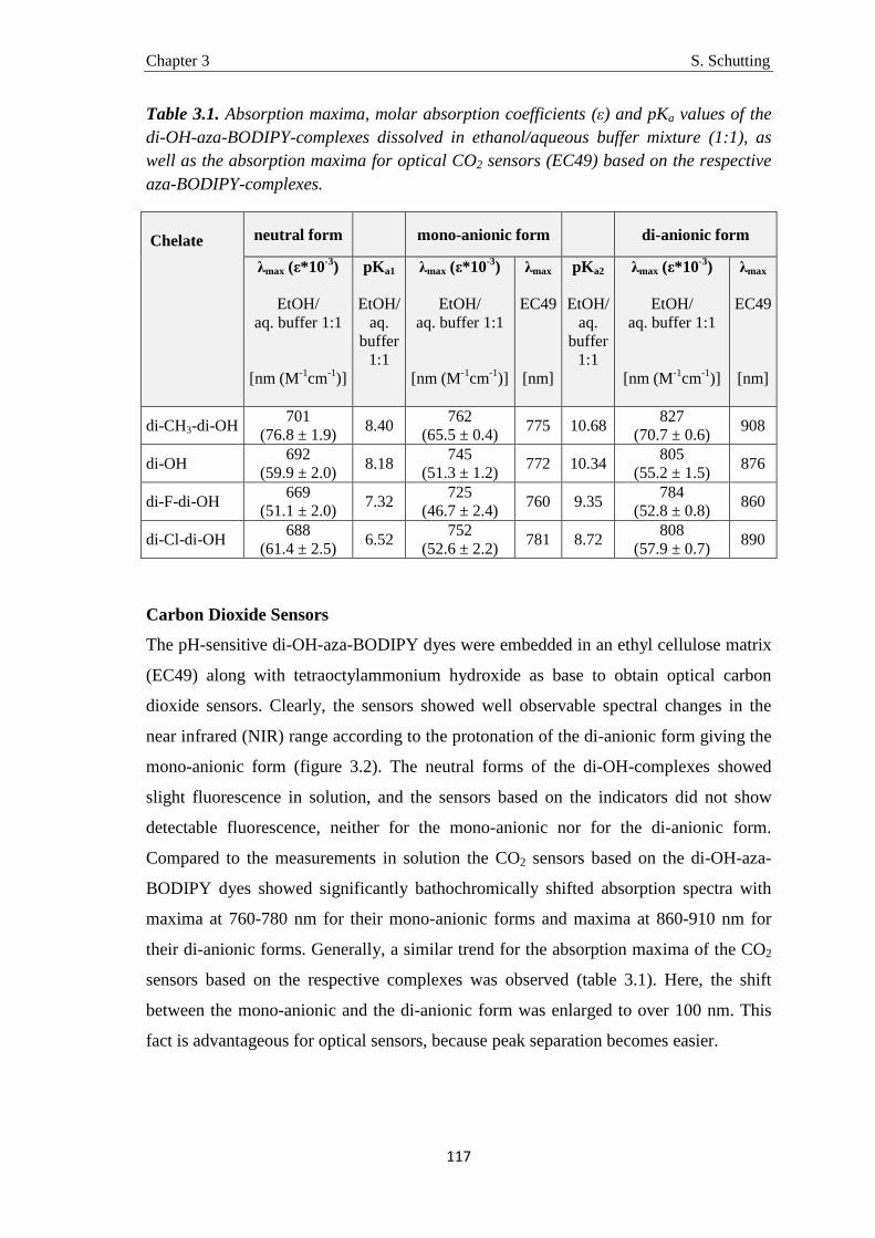
Chapter 3 S. Schutting
117
Table 3.1. Absorption maxima, molar absorption coefficients (ε) and pKa values of the di-OH-aza-BODIPY-complexes dissolved in ethanol/aqueous buffer mixture (1:1), as well as the absorption maxima for optical CO2 sensors (EC49) based on the respective aza-BODIPY-complexes.
Chelate neutral form
mono-anionic form
di-anionic form
λmax (ε*10-3)
EtOH/ aq. buffer 1:1
[nm (M-1cm-1)]
pK a1
EtOH/ aq.
buffer 1:1
λmax (ε*10-3)
EtOH/ aq. buffer 1:1
[nm (M-1cm-1)]
λmax
EC49
[nm]
pK a2
EtOH/ aq.
buffer 1:1
λmax (ε*10-3)
EtOH/ aq. buffer 1:1
[nm (M-1cm-1)]
λmax
EC49
[nm]
di-CH3-di-OH 701
(76.8 ± 1.9) 8.40
762 (65.5 ± 0.4)
775 10.68 827
(70.7 ± 0.6) 908
di-OH 692
(59.9 ± 2.0) 8.18
745 (51.3 ± 1.2)
772 10.34 805
(55.2 ± 1.5) 876
di-F-di-OH 669
(51.1 ± 2.0) 7.32
725 (46.7 ± 2.4)
760 9.35 784
(52.8 ± 0.8) 860
di-Cl-di-OH 688
(61.4 ± 2.5) 6.52
752 (52.6 ± 2.2)
781 8.72 808
(57.9 ± 0.7) 890
Carbon Dioxide Sensors
The pH-sensitive di-OH-aza-BODIPY dyes were embedded in an ethyl cellulose matrix
(EC49) along with tetraoctylammonium hydroxide as base to obtain optical carbon
dioxide sensors. Clearly, the sensors showed well observable spectral changes in the
near infrared (NIR) range according to the protonation of the di-anionic form giving the
mono-anionic form (figure 3.2). The neutral forms of the di-OH-complexes showed
slight fluorescence in solution, and the sensors based on the indicators did not show
detectable fluorescence, neither for the mono-anionic nor for the di-anionic form.
Compared to the measurements in solution the CO2 sensors based on the di-OH-aza-
BODIPY dyes showed significantly bathochromically shifted absorption spectra with
maxima at 760-780 nm for their mono-anionic forms and maxima at 860-910 nm for
their di-anionic forms. Generally, a similar trend for the absorption maxima of the CO2
sensors based on the respective complexes was observed (table 3.1). Here, the shift
between the mono-anionic and the di-anionic form was enlarged to over 100 nm. This
fact is advantageous for optical sensors, because peak separation becomes easier.

Chapter 3 S. Schutting
118
600 700 800 900 10000.0
0.2
0.4
0.6
0.8
600 700 800 900 10000.0
0.2
0.4
0.6
0.8
Abs
orba
nce
Wavelength (nm)
N2
2.5 kPa CO2
7.1 kPa CO2
14.6 kPa CO2
31.2 kPa CO2
98.1 kPa CO2
A
BAbs
N2
0.04 kPa CO2
0.1 kPa CO2
0.2 kPa CO2
0.5 kPa CO2
4.9 kPa CO2
Abs
orba
nce
Wavelength (nm)
Abs0
Figure 3.2. Absorption spectra of optical carbon dioxide sensors based on (A) the di-Cl-di-OH-complex and (B) the di-CH3-di-OH-complex in EC49 (base: TOAOH) at 25°C at various pCO2 values.
Despite that all di-OH-aza-BODIPY dyes showed two protonation steps in aqueous
solution, only one protonation step was observed in optical sensors based on these
indicators. In fact, in absence of carbon dioxide both hydroxyl groups build ion pairs
with the quaternary ammonium base and the spectra for the di-anionic forms are
observable. The mono-anionic form is built in presence of carbon dioxide and is stable
even at 100% CO2. Spectra for the neutral forms are not observable anymore (figure
3.2). Therefore, the pKa2 values measured in solution are most relevant for optical
carbon dioxide sensors based on the di-OH-aza-BODIPY dyes. Indeed, these values
correlate very well with the sensitivities of the optical CO2 sensors (table 3.1, figure
3.3). The sensitivity increases in the following order: di-Cl-di-OH < di-F-di-OH < di-
OH < di-CH3-di-OH. Notably, for the most sensitive sensor based on di-CH3-di-OH

Chapter 3 S. Schutting
119
about 25% of the overall signal change is observed already at atmospheric pCO2 which
is, to the best of our knowledge, one of the highest sensitivities reported so far. Di-F-di-
OH and di-Cl-di-OH complexes bearing electron-withdrawing groups displayed
diminished pKa2 values of 9.35 and 8.72, respectively, and enabled measurements up to
100% CO2. These great differences in sensitivity lead to a broad range of applications,
varying from food packaging and capnography for di-F-di-OH and di-Cl-di-OH
complexes to environmental monitoring for di-OH and di-CH3-di-OH complexes.
Figure 3.3 shows the increasing absorption of the mono-anionic form in relation to the
absorption at 0 kPa (Abs-Abs0) carbon dioxide (see figure 3.2 B). The higher the
sensitivity of the sensor, the steeper the respective calibration curves in figure 3.3 and
the lower the amount of carbon dioxide necessary to fully protonate the sensor. Sensors
based on the di-Cl-di-OH-complex and the di-F-di-OH-complex showed limits of
detection (LOD) of 0.19 kPa and 0.18 kPa, respectively. However, determining the
LOD value for very sensitive sensors can be very challenging. For measurements of low
levels of carbon dioxide the measuring system (gas mixer, gas lines, flow cell, etc.) has
to be completely decarbonized, which is very difficult to achieve in reality. Especially
for atmospheric levels of pCO2 (0.04 kPa ≈ 400 µatm in the gas phase ≈ 11.6 µmol l-1 in
water at 298.15 K) and below, traces of environmental carbon dioxide disturbed the
measurements for sensors based on the di-CH3-di-OH-complex and the di-OH-complex.
Hence, the determined LODs for these two complexes (0.011 kPa for di-OH and 0.007
kPa for di-CH3-di-OH) were only rough estimations.

Chapter 3 S. Schutting
120
0 1 2 3 4 5
0.0
0.1
0.2
0.3
0.4
0.0 0.2 0.4 0.6
0.0
0.1
0.2
0.3
0 20 40 60 80 100
0.0
0.1
0.2
0.3
0 2 4 6 8 10
0.0
0.1
di-OHA
bs
- A
bs 0
pCO2 (kPa)
di-CH3-di-OH
A
di-OH
Ab
s -
Ab
s 0
pCO2 (kPa)
di-CH3-di-OHC
DB di-F-di-OH
Ab
s -
Ab
s 0
pCO2 (kPa)
di-Cl-di-OH
di-F-di-OH
Ab
s -
Ab
s 0
pCO2 (kPa)
di-Cl-di-OH
Figure 3.3. (A) Calibration curves (absorption – absorption at 0 kPa of the mono-anionic form) for the carbon dioxide sensors based on di-OH-complex (black) and di-CH3-di-OH-complex (green) and (B) di-Cl-di-OH-complex (blue) and di-F-di-OH-complex (red) 25°C under humid conditions with the respective “zoom-in” sections (C and D).
Photodegradation profiles of the carbon dioxide sensors were obtained from the
absorption spectra after illuminating the sensor foils with a high-power LED array (λmax
458 nm). For comparison, state-of-the-art indicator dyes such as m-cresol-purple,
thymol-blue and HPTS were used (supporting information, figure S3.1). The
photostability of both the mono-anionic and the di-anionic form were investigated.
Therefore, the cuvette was filled either with pure carbon dioxide (mono-anionic form)
or with pure nitrogen (di-anionic form). Clearly, all of the di-OH-aza-BODIPY dyes
showed outstanding photostability, much better than the reference indicators embedded
in the same ethyl cellulose matrix. After 1.5 h of illumination the presented dyes
showed hardly any photobleaching effects for both the mono-anionic and di-anionic
form, whereas m-cresol-purple (neutral form), thymol-blue (neutral form) and HPTS
(only anionic form) were degraded to less than 80%. The anionic forms of m-cresol-
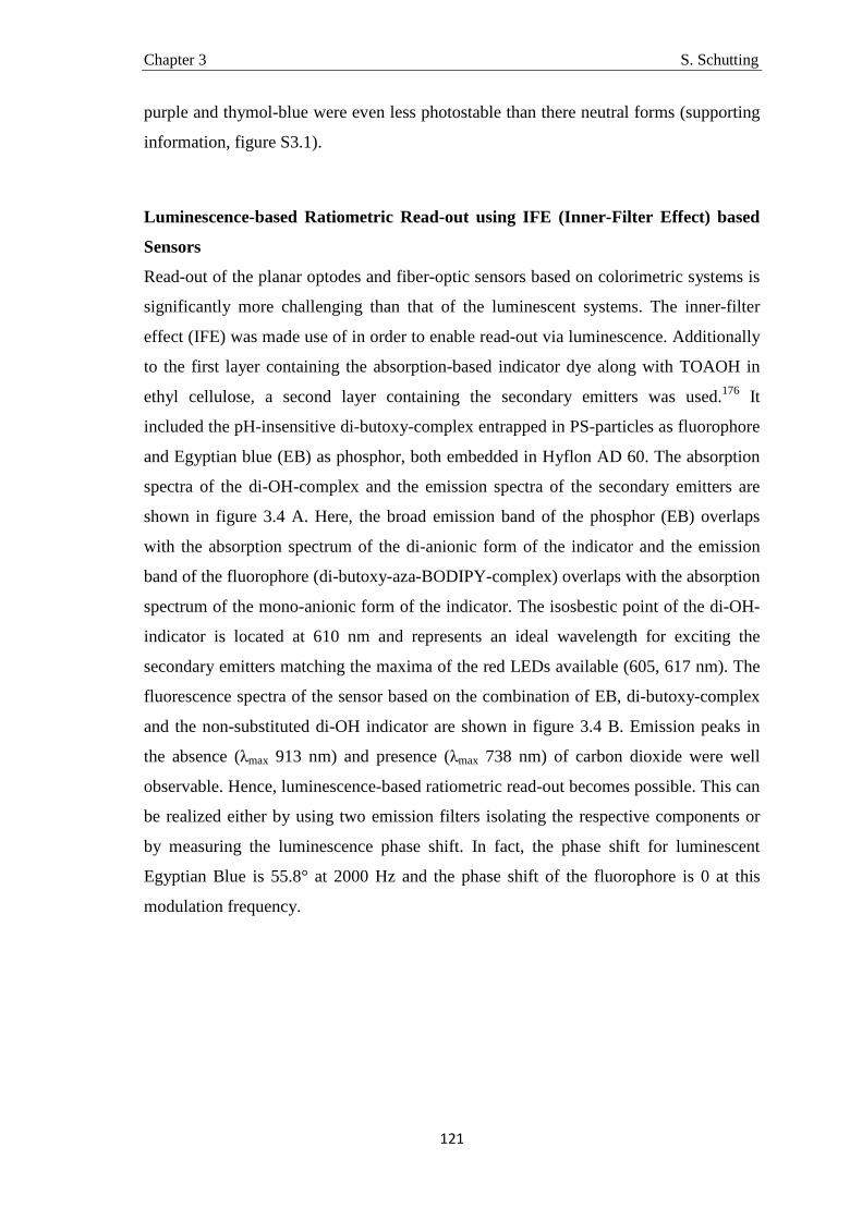
Chapter 3 S. Schutting
121
purple and thymol-blue were even less photostable than there neutral forms (supporting
information, figure S3.1).
Luminescence-based Ratiometric Read-out using IFE (Inner-Filter Effect) based
Sensors
Read-out of the planar optodes and fiber-optic sensors based on colorimetric systems is
significantly more challenging than that of the luminescent systems. The inner-filter
effect (IFE) was made use of in order to enable read-out via luminescence. Additionally
to the first layer containing the absorption-based indicator dye along with TOAOH in
ethyl cellulose, a second layer containing the secondary emitters was used.176 It
included the pH-insensitive di-butoxy-complex entrapped in PS-particles as fluorophore
and Egyptian blue (EB) as phosphor, both embedded in Hyflon AD 60. The absorption
spectra of the di-OH-complex and the emission spectra of the secondary emitters are
shown in figure 3.4 A. Here, the broad emission band of the phosphor (EB) overlaps
with the absorption spectrum of the di-anionic form of the indicator and the emission
band of the fluorophore (di-butoxy-aza-BODIPY-complex) overlaps with the absorption
spectrum of the mono-anionic form of the indicator. The isosbestic point of the di-OH-
indicator is located at 610 nm and represents an ideal wavelength for exciting the
secondary emitters matching the maxima of the red LEDs available (605, 617 nm). The
fluorescence spectra of the sensor based on the combination of EB, di-butoxy-complex
and the non-substituted di-OH indicator are shown in figure 3.4 B. Emission peaks in
the absence (λmax 913 nm) and presence (λmax 738 nm) of carbon dioxide were well
observable. Hence, luminescence-based ratiometric read-out becomes possible. This can
be realized either by using two emission filters isolating the respective components or
by measuring the luminescence phase shift. In fact, the phase shift for luminescent
Egyptian Blue is 55.8° at 2000 Hz and the phase shift of the fluorophore is 0 at this
modulation frequency.
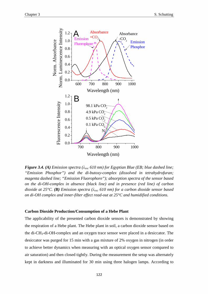
Chapter 3 S. Schutting
122
600 700 800 900 10000.0
0.2
0.4
0.6
0.8
1.0
1.2
700 800 900 10000.0
0.2
0.4
0.6
0.8
1.0
1.2 B
No
rm. A
bso
rban
ceN
orm
. Lu
min
esce
nce
Inte
nsi
ty
Wavelength (nm)
Emission Fluorophore Emission
Phosphor
Absorbance+CO
2
Absorbance-CO
2
A
98.1 kPa CO2
4.9 kPa CO2
0.5 kPa CO2
0.1 kPa CO2
N2
Flu
ore
scen
ce In
ten
sity
Wavelength (nm)
Figure 3.4. (A) Emission spectra (λexc 610 nm) for Egyptian Blue (EB; blue dashed line; “Emission Phosphor”) and the di-butoxy-complex (dissolved in tetrahydrofuran; magenta dashed line; “Emission Fluorophore”); absorption spectra of the sensor based on the di-OH-complex in absence (black line) and in presence (red line) of carbon dioxide at 25°C. (B) Emission spectra (λexc 610 nm) for a carbon dioxide sensor based on di-OH complex and inner-filter effect read-out at 25°C and humidified conditions.
Carbon Dioxide Production/Consumption of a Hebe Plant
The applicability of the presented carbon dioxide sensors is demonstrated by showing
the respiration of a Hebe plant. The Hebe plant in soil, a carbon dioxide sensor based on
the di-CH3-di-OH-complex and an oxygen trace sensor were placed in a desiccator. The
desiccator was purged for 15 min with a gas mixture of 2% oxygen in nitrogen (in order
to achieve better dynamics when measuring with an optical oxygen sensor compared to
air saturation) and then closed tightly. During the measurement the setup was alternately
kept in darkness and illuminated for 30 min using three halogen lamps. According to
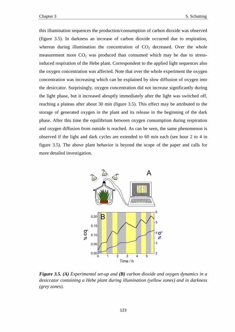
Chapter 3 S. Schutting
123
this illumination sequences the production/consumption of carbon dioxide was observed
(figure 3.5). In darkness an increase of carbon dioxide occurred due to respiration,
whereas during illumination the concentration of CO2 decreased. Over the whole
measurement more CO2 was produced than consumed which may be due to stress-
induced respiration of the Hebe plant. Correspondent to the applied light sequences also
the oxygen concentration was affected. Note that over the whole experiment the oxygen
concentration was increasing which can be explained by slow diffusion of oxygen into
the desiccator. Surprisingly, oxygen concentration did not increase significantly during
the light phase, but it increased abruptly immediately after the light was switched off,
reaching a plateau after about 30 min (figure 3.5). This effect may be attributed to the
storage of generated oxygen in the plant and its release in the beginning of the dark
phase. After this time the equilibrium between oxygen consumption during respiration
and oxygen diffusion from outside is reached. As can be seen, the same phenomenon is
observed if the light and dark cycles are extended to 60 min each (see hour 2 to 4 in
figure 3.5). The above plant behavior is beyond the scope of the paper and calls for
more detailed investigation.
Figure 3.5. (A) Experimental set-up and (B) carbon dioxide and oxygen dynamics in a desiccator containing a Hebe plant during illumination (yellow zones) and in darkness (grey zones).

Chapter 3 S. Schutting
124
Conclusion
A new class of colorimetric pH-sensitive indicators for carbon dioxide sensors is
presented. The di-OH-aza-BODIPY dyes show characteristic CO2-dependent absorption
spectra in the near-infrared region. In addition to the remarkable photostability of the
indicators and the high molar absorption coefficients, the dynamic ranges of the sensors
can be tuned via electron-donating and electron-withdrawing substituents. This enables
a broad range of applications from environmental monitoring to food packaging or
capnography. The sensors based on di-CH3-di-OH-aza-BODIPY belong to the most
sensitive ever reported and resolve well below atmospheric CO2 levels. Absorption-
modulated inner-filter effect was used to enable referenced luminescence-based
ratiometric read-out. As an example the production/consumption of carbon dioxide of a
Hebe plant was demonstrated.
Acknowledgment
This work was supported by 7th framework EU projects ECO2 (project number
265847) and SenseOCEAN (project number 614141).

Chapter 3 S. Schutting
125
Supporting Information
to NIR Optical Carbon Dioxide Sensors Based on Highly Photostable Dihydroxy-aza-BODIPY Dyes
0 20 40 60 80
50
60
70
80
90
100
Dye
am
ou
nt (
%)
Time (min)
HPTS(deprot)
Thymol-blue(prot)
m-Cresol-purple(prot)
Figure S3.1. Photodegradation profiles for carbon dioxide sensors (EC49; base: TOAOH; T=25°C) based on the di-OH-aza-BODIPY dyes (black), m-cresol-purple (red triangles), thymol-blue (green dots) obtained from the absorption spectra of the respective neutral form and the absorption spectra of the deprotonated forms of the di-Cl-di-OH-complex (cyan) and HPTS(TOA)3 (blue stars).

Chapter 3 S. Schutting
126
Figure S3.2. EI-DI Mass spectrum of 3,7-bis(4-butoxyphenyl)-5,5-difluoro-1,9-diphenyl-5H-4λ4,5λ4-dipyrrolo[1,2-c:2',1'-ƒ][1,3,5,2]triazaborinine (di-butoxy-complex).
m/z60 80 100 120 140 160 180 200 220 240 260 280 300 320 340 360 380 400 420 440 460 480 500 520 540 560 580 600 620 640 660
%
0
100
Strobl Dibutoxy-Komplex 198 (3.300) AM (Cen,2, 70.00, Ht,6800.0,0.00,0.70); Sm (SG, 1x3.00); Cm (172:198-1:38) TOF MS EI+ 1.74e4641.3
528.2
64.0
57.1
527.2
77.0 119.0105.0177.1 500.2204.1 232.1
529.2
640.3
584.2
530.2
585.3
586.3
642.3
643.3
m/z634 635 636 637 638 639 640 641 642 643 644 645 646 647 648 649 650 651 652
%
0
100
%
0
100
Strobl Dibutoxy-Komplex (0.017) Is (0.10,0.01) C40H38BF2N3O2 TOF MS EI+ 5.62e12641.3032
640.3062
642.3062
643.3091
Strobl Dibutoxy-Komplex 198 (3.300) AM (Cen,2, 70.00, Ht,6800.0,0.00,0.70); Sm (SG, 1x3.00); Cm (172:198-1:38) TOF MS EI+ 1.74e4641.3007
640.3057
642.3071
643.3129
Theoretical isotope pattern M+
Experimental
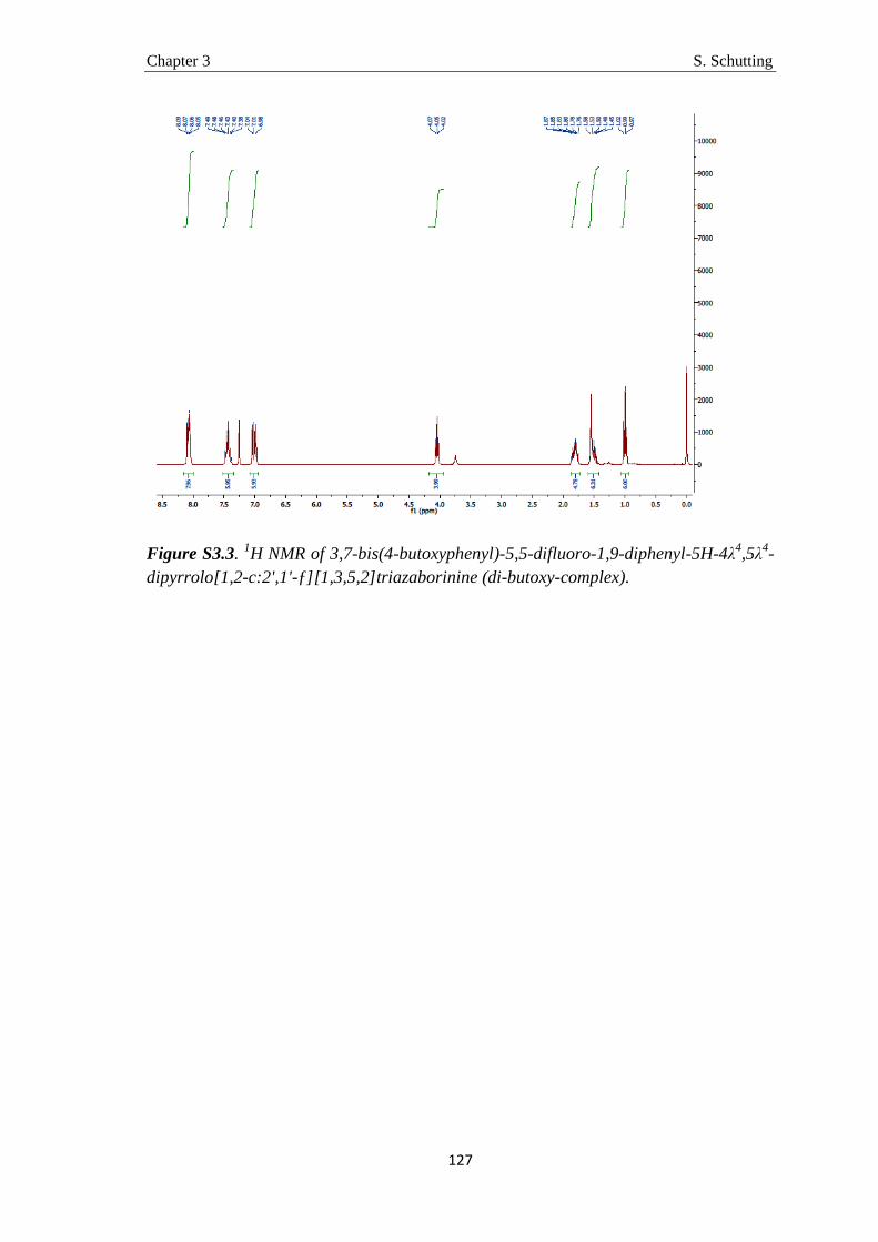
Chapter 3 S. Schutting
127
Figure S3.3. 1H NMR of 3,7-bis(4-butoxyphenyl)-5,5-difluoro-1,9-diphenyl-5H-4λ4,5λ4-dipyrrolo[1,2-c:2',1'-ƒ][1,3,5,2]triazaborinine (di-butoxy-complex).

Chapter 3 S. Schutting
128
Figure S3.4. EI-DI Mass spectrum of 4,4'-(5,5-difluoro-1,9-diphenyl-5H-4λ4,5λ4-dipyrrolo[1,2-c:2',1'-ƒ][1,3,5,2]triazaborinine-3,7-diyl)diphenol (di-OH-complex).
m/z50 100 150 200 250 300 350 400 450 500 550 600 650 700 750 800
%
0
100
%
0
100
Schutting_di-OH-complex_ b (0.017) Is (0.05,1.00) C32H22BF2N3O2 TOF MS EI+ 6.02e12529.1779
528.1810
530.1808
531.1838
Schutting_di-OH-complex_ b 88 (1.467) Cm (84:90-61:73) TOF MS EI+ 977529.1771
121.0306104.0263 528.1793
122.0983264.5829207.0804
232.0803 265.0973 481.1893361.1349 378.1666
530.1805
531.1847575.9734
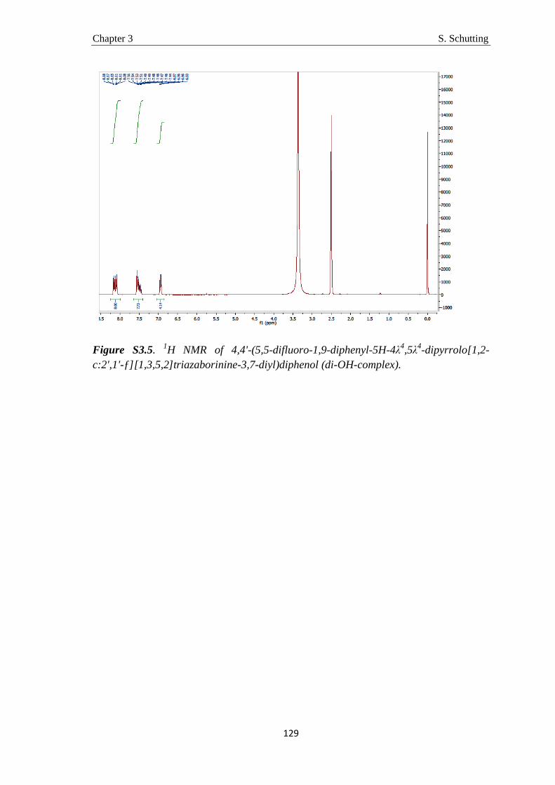
Chapter 3 S. Schutting
129
Figure S3.5. 1H NMR of 4,4'-(5,5-difluoro-1,9-diphenyl-5H-4λ4,5λ4-dipyrrolo[1,2-c:2',1'-ƒ][1,3,5,2]triazaborinine-3,7-diyl)diphenol (di-OH-complex).

Chapter 3 S. Schutting
130
Figure S3.6. DI-EI Mass spectrum of 4,4'-(5,5-difluoro-1,9-diphenyl-5H-4λ4,5λ4-dipyrrolo[1,2-c:2',1'-ƒ][1,3,5,2]triazaborinine-3,7-diyl)bis(3-fluorophenol) (di-F-di-OH-complex).
m/z60 80 100 120 140 160 180 200 220 240 260 280 300 320 340 360 380 400 420 440 460 480 500 520 540 560 580 600
%
0
100
Strobl Probe 1 123 (2.050) Cm (123:126-106:111) TOF MS EI+ 1.34e3565.2
564.2
250.176.0 103.079.0 137.0230.1202.1
282.6265.1
566.2
567.2
m/z548 550 552 554 556 558 560 562 564 566 568 570 572 574 576 578 580 582 584 586
%
0
100
%
0
100
Strobl Probe 1 (0.017) Is (0.10,0.01) C32H20BF4N3O2 TOF MS EI+ 6.03e12565.1591
564.1621
566.1620
567.1649
Strobl Probe 1 123 (2.050) Cm (123:126-106:111) TOF MS EI+ 1.34e3565.1615
564.1620
566.1672
567.1647
Theoretical isotope pattern M+
Experimental

Chapter 3 S. Schutting
131
Figure S3.7. 1H NMR of 4,4'-(5,5-difluoro-1,9-diphenyl-5H-4λ4,5λ4-dipyrrolo[1,2-c:2',1'-ƒ][1,3,5,2]triazaborinine-3,7-diyl)bis(3-fluorophenol) (di-F-di-OH-complex).
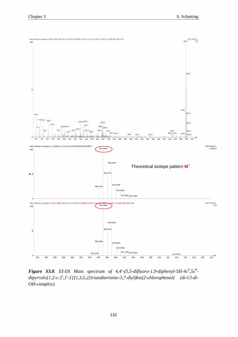
Chapter 3 S. Schutting
132
Figure S3.8. EI-DI Mass spectrum of 4,4'-(5,5-difluoro-1,9-diphenyl-5H-4λ4,5λ4-dipyrrolo[1,2-c:2',1'-ƒ][1,3,5,2]triazaborinine-3,7-diyl)bis(2-chlorophenol) (di-Cl-di-OH-complex).
m/z60 80 100 120 140 160 180 200 220 240 260 280 300 320 340 360 380 400 420 440 460 480 500 520 540 560 580 600 620
%
0
100
Jokic dichloro complex 4 96 (1.600) AM (Cen,4, 60.00, Ht,6800.0,0.00,0.70); Sm (SG, 1x3.00); Cm (95:100-104:110) TOF MS EI+ 750597.1
596.1
60.0
85.077.0
72.1
105.0
86.1
219.1
118.1155.0
141.1
163.1
218.1202.1
176.1
228.0299.0
232.1298.5
241.0 295.1258.1
299.5
319.1 549.1324.1 548.1
395.1341.1
423.1 470.1552.1 595.1
599.1
600.1
601.1
602.1
603.1
m/z582 584 586 588 590 592 594 596 598 600 602 604 606 608 610 612 614 616 618 620 622
%
0
100
%
0
100
Jokic dichloro complex 4 (0.083) Is (0.10,0.01) C32H20Cl2N3O2BF2 TOF MS EI+ 3.46e12597.0999
596.1030
599.0978
598.1021
600.1000
601.0967
602.0981 603.1006
Jokic dichloro complex 4 96 (1.600) AM (Cen,4, 60.00, Ht,6800.0,0.00,0.70); Sm (SG, 1x3.00); Cm (95:100-104:110) TOF MS EI+ 750597.0968
596.0994
595.1038
599.0932
598.1002
600.0955
601.0992
602.1005 603.0959613.9741
Theoretical isotope pattern M+
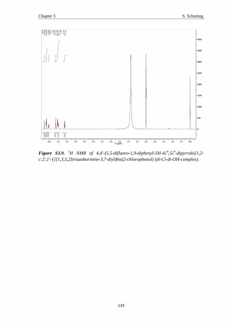
Chapter 3 S. Schutting
133
Figure S3.9. 1H NMR of 4,4'-(5,5-difluoro-1,9-diphenyl-5H-4λ4,5λ4-dipyrrolo[1,2-c:2',1'-ƒ][1,3,5,2]triazaborinine-3,7-diyl)bis(2-chlorophenol) (di-Cl-di-OH-complex).

Chapter 3 S. Schutting
134
Figure S3.10. EI-DI Mass spectrum of 4,4'-(5,5-difluoro-1,9-diphenyl-5H-4λ4,5λ4-dipyrrolo[1,2-c:2',1'-ƒ][1,3,5,2]triazaborinine-3,7-diyl)bis(2-methylphenol) (di-CH3-di-OH-complex).
m/z50 75 100 125 150 175 200 225 250 275 300 325 350 375 400 425 450 475 500 525 550 575 600
%
0
100
%
0
100
Schutting_di_CH3_di_OH_complex_b (0.017) Is (0.05,1.00) C34H26N3O2BF2 TOF MS EI+ 5.92e12557.2092
556.2122
558.2122
559.2151
Schutting_di_CH3_di_OH_complex_b 121 (2.017) Cm (121:126-98:107) TOF MS EI+ 1.28e3557.2082
69.0701 122.0933
134.0574556.2123
239.2401
229.1105137.1286
192.1776
319.3266
299.2628276.2725
327.2932
355.0738 429.0912 509.1943444.4307
558.2112
559.2184
614.9946
Theoretical isotope pattern M+
Experimental
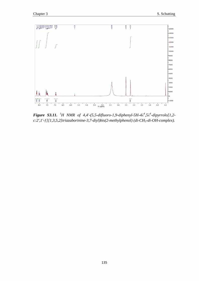
Chapter 3 S. Schutting
135
Figure S3.11. 1H NMR of 4,4'-(5,5-difluoro-1,9-diphenyl-5H-4λ4,5λ4-dipyrrolo[1,2-c:2',1'-ƒ][1,3,5,2]triazaborinine-3,7-diyl)bis(2-methylphenol) (di-CH3-di-OH-complex).

Chapter 3 S. Schutting
136

Chapter 4 S. Schutting
137
Chapter 4
Scope of this chapter
In chapter 4 a possible application of optical carbon dioxide sensors in marine
environments is presented. The device was constructed to especially meet the demands
of field experiments in marine science, where time, staff, and equipment are limited. It
should give as much simultaneous information as possible concerning spatial and
temporal distribution of the analyte concentration. Thus, one hundred optical fiber
sensors for carbon dioxide with one collective excitation source and imaging read-out
were attached to the housing containing the RGB camera and the electronics.
Characterization of the device was first carried out under lab conditions.
Afterwards, the prototype was tested under real conditions off Panarea Island (Sicily,
Italy). Panarea Island is located in the southern Tyrrhenian Sea north of Sicily and is
known to be in a volcanically active area, as for example in 2002 a huge underwater
outbreak of carbon dioxide occurred and still carbon dioxide is outgasing there from the
seafloor. It is not yet definitely known if the CO2 reaches the seawater either
continuously and point-by-point via bubbles, or discontinuously via tidally affected
pore-water dynamics. To answer this question, the multi-branched sensor device was
applied off Panarea Island (Sicily, Italy).

Chapter 4 S. Schutting
138
Chapter 4 S. Schutting
139
Multi-Branched Optical Carbon Dioxide Sensors for Marine Applications
The distribution of CO2 in natural waters can vary significantly within small areas due
to physical, chemical and biological processes. To achieve more information about
these systems, simultaneous detection of CO2 concentration at many different positions
is highly desired. In this contribution a multi-branched optical carbon dioxide sensor
system is presented. The ends of 100 optical fibers are coated with optical carbon
dioxide sensing foils, which – after excitation – emit light in either the red or the green
part of the spectrum according to the ambient pCO2. These ends are freely moveable,
whereas the opposite ends are reunited in a polished fiber head building a 10 x 10
matrix of fiber spots. This fiber head is positioned in front of a commercially available
red/green/blue (RGB) camera, which enables read-out via imaging. Images are then
divided in their color channels, which contain the analytical information. Here, the
intensity in the red and green channel is used (ratio red/green). The system was tested
off Panarea Island (Sicily, Italy), which is located in the Tyrrhenian Sea in a
volcanically active area, where carbon dioxide is outgasing from the seafloor. A
significant effect of tides, but no correlation with photosynthesis was observed via the
measured CO2 dynamics.
Introduction
It is known that increasing carbon dioxide concentrations in the atmosphere cause
elevated CO2 levels in the oceans. Marine scientists are investigating this phenomenon -
also known as ocean acidification - and its strong effects on the marine ecosystem.9,181–
186 Therefore, an appropriate detection method is necessary. Especially for field
experiments where time, equipment and staff are limited, it is important that the method
is easily adaptable to the respective conditions of the experiment and that it gives as
much simultaneous information as possible concerning spatial and temporal distribution
of the analyte concentration.
Chapter 4 S. Schutting
140
Optical chemosensors116–118,139,140 are ascending and promising detection tools for
analytes such as pH,143,150,152,187–189 oxygen155,190–193 or carbon
dioxide.61,92,111,132,167,171,194 The most common ones for carbon dioxide are so called
plastic type sensors51,65,66,89,112,113 with a pH-sensitive indicator dye as core-component
of the sensing film. The indicator shows changing spectral properties – absorption
and/or luminescence properties – due to its degree of protonation. If an experiment
requires a certain mobility of the sensor, to measure in small volumes, to be non-invasiv
or to overcome a certain distance, the application of fiber optodes195–198 becomes
preferable. Here, optical fibers, either made of glass or polymer, guide the excitation
light to the sensing element (foil or coated tip) and the emitted light back. If
simultaneous detection at more than one measurement point is required, those optical
fibers can also be used in so called multi-fiber arrays.190,199,200
In 2012 Fischer and Koop-Jakobsen published the multiple fiber optode (MuFO), a
novel system for simultaneous analysis of multiple fiber optic oxygen sensors.201 The
device was based on simultaneous lifetime imaging of optical sensing foils, which were
based on the principle of oxygen quenching of a fluorescent indicator dye enabling
measurements at 100 positions at the same time. As the used principle was not
applicable for carbon dioxide, the read-out method had to be adapted for optical CO2
sensors, which are based on a pH-sensitive indicator dye. Here, an enhancement of the
previous device, enabling simultaneous interrogation of one hundred optical carbon
dioxide fiber optodes based on imaging read-out, is presented.
Experimental
Materials
Ethyl cellulose (EC49, ethoxyl content 49%), thymol-blue (A.C.S. reagent), m-cresol-
purple (indicator grade) and tetraoctylammonium hydroxide solution (TOAOH, 20% in
methanol) were obtained from Sigma-Aldrich (www.sigmaaldrich.com). Nitrogen, 5%
carbon dioxide in nitrogen, 0.2% carbon dioxide in nitrogen, argon and carbon dioxide
(all of 99.9990% purity) were obtained from Air Liquide (Austria, www.airliquide.at).
Toluene, ethanol (EtOH), sodium chloride, sodium bicarbonate and hexane were
purchased from VWR (Austria, www.vwr.com). Poly(ethylene terephthalate) (PET)

Chapter 4 S. Schutting
141
support Melinex 505 was obtained from Pütz (Germany, www.puetz-folien.com). The
buffer salts di-sodium phosphate (≥ 99%, p.a.) and monopotassium phosphate (p.a.)
were purchased from ROTH (www.carlroth.com) and MERCK (www.merck.at),
respectively. The silicone components vinyl terminated polydimethylsiloxane (viscosity
1000 cSt.), (25-35% methylhydrosiloxane)-dimethylsiloxane copolymer (viscosity 25-
35 cSt.), 1,3,5,7-tetravinyl-1,3,5,7-tetramethylcyclotetrasiloxanen and the platinum-
divinyltetramethyldisiloxane complex were received from ABCR (Germany,
www.abcr.de). The pigments brick-red and lemon-yellow were purchased from Kremer
Pigments (Germany, www.kremer-pigmente.com). Black silicone-rubber ELASTOSIL
N189 was obtained from Wacker (www.wacker.com). De-ionized water was filtered via
a Barnstead NANOpure ultrapure water system. The optical plastic fibers LUMINOUS
(type C-1000; Ø 2.2 mm) from Asahi Chemical Japan were ordered via Sojitz Europe
plc. (www.sojitz.de). The material for the metal sleeves, a stainless steel pipe (inner
Ø2.2 mm; type 1.4571), was purchased from SW-Stahl (www.sw-stahl.de). The RGB
camera (type EOS 1000D, internal infrared filter removed) and the objective (type EF-S
60 mm) were from Canon (www.canon.at). A SDHC card (32 GB) from Sandisk
(www.sandisk.de) was used for image-storage during the measurements. LEDs (type
LUXEON Rebel LXML PB01 0030, blue 470 nm, 75l m; incl. LED star board) were
purchased from LUMITRONIX LED-Technik GmbH (www.leds.de) and the respective
LED driver from PCB components (www.pcb-components.de). Optical filter DT-Blue
and the NIR blocking filter Calflex X were obtained from Qioptiq (www.qioptiq-
shop.com). A 500 nm long pass filter from Schott (www.schott.com) and a LEE plastic
filter (medium yellow; www.leefilters.com) were used in front of the camera. The
material for the housing and the fiber head ERTACETAL (POM C, Polyoxymethylen)
was purchased from ARTHUR KRÜGER GmbH (www.arthur-krueger.de). The cutting
pliers Rennsteig 600 001 3 was obtained from (www.rennsteig.com/de). Electronics:
USB/ LAN converter (4x) was received from Sharkoon (www.sharkoon.com) and the
LAN switch (FS105 5 Port 10/100MBit) from Netgear (www.netgear.at). Accumulator
packs 4x 16Ah 3.2C cells (Headway 40160SE) were obtained from Lipopower
(www.lipopower.de).
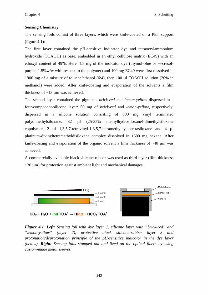
Chapter 4 S. Schutting
142
Sensing Chemistry
The sensing foils consist of three layers, which were knife-coated on a PET support
(figure 4.1):
The first layer contained the pH-sensitive indicator dye and tetraoctylammonium
hydroxide (TOAOH) as base, embedded in an ethyl cellulose matrix (EC49) with an
ethoxyl content of 49%. Here, 1.5 mg of the indicator dye (thymol-blue or m-cresol-
purple; 1.5%w/w with respect to the polymer) and 100 mg EC49 were first dissolved in
1900 mg of a mixture of toluene/ethanol (6:4), then 100 µl TOAOH solution (20% in
methanol) were added. After knife-coating and evaporation of the solvents a film
thickness of ~13 µm was achieved.
The second layer contained the pigments brick-red and lemon-yellow dispersed in a
four-component-silicone layer: 50 mg of brick-red and lemon-yellow, respectively,
dispersed in a silicone solution consisting of 800 mg vinyl terminated
polydimethylsiloxane, 32 µl (25-35% methylhydrosiloxane)-dimethylsiloxane
copolymer, 2 µl 1,3,5,7-tetravinyl-1,3,5,7-tetramethylcyclotetrasiloxane and 4 µl
platinum-divinyltetramethyldisiloxane complex dissolved in 1600 mg hexane. After
knife-coating and evaporation of the organic solvent a film thickness of ~40 µm was
achieved.
A commercially available black silicone-rubber was used as third layer (film thickness
~30 µm) for protection against ambient light and mechanical damages.
Figure 4.1. Left: Sensing foil with dye layer 1, silicone layer with “brick-red” and “lemon-yellow” (layer 2), protective black silicone-rubber layer 3 and protonation/deprotonation principle of the pH-sensitive indicator in the dye layer (below). Right: Sensing foils stamped out and fixed on the optical fibers by using custom-made metal sleeves.

Chapter 4 S. Schutting
143
Methods
Characterization of the sensing chemistry: Absorption spectra were recorded on a Cary
50 UV-vis spectrophotometer (www.varianinc.com). Photobleaching experiments were
performed by irradiating the sensor foils in a glass cuvette with light of a high-power 10
W LED array (λmax 458 nm, 3 LEDs, LED-TECH.de) operated at 6 W input power. A
lens (Edmund Optics) was used to focus the light of the LED array on the glass cuvette
(photon flux: ~3900 µmol s-1 m-2 as determined with a Li-250A light meter from Li-
COR). The photodegradation profiles were obtained by monitoring the absorption
spectra of a sensor foil based on the respective dye. The cuvette was flushed with either
carbon dioxide gas for the protonated form, or with nitrogen for the deprotonated form
and sealed with Parafilm. Fluorescence intensity measurements of the sensing foils were
recorded on a Hitachi F-7000 Fluorescence spectrometer (www.hitachi.com) equipped
with a red-sensitive photomultiplier R928 from Hamamatsu (www.hamamatsu.com).
Gas calibration mixtures were obtained using a gas mixing device from MKS
(www.mksinst.com). The gas mixture was humidified to about 85% relative humidity
(saturated KCl solution) prior entering the calibration chamber. Temperature was
controlled by a cryostat ThermoHaake DC50. The phosphate buffer solution (~700 mM)
was composed of 13.60 g di-sodium phosphate, 0.72 g monopotassium phosphate and
35.06 g sodium chloride dissolved in 1000 ml of de-ionized water and showed a pH
value of 7.7-7.8. Calibration measurements were carried out by flushing the phosphate
buffer solution first with pure nitrogen gas until a plateau was reached. Afterwards a
solution of 1.59 g sodium bicarbonate dissolved in 50 ml of de-ionized water was added
stepwise to give increasing levels of carbon dioxide concentration.
The multi-branched optical carbon dioxide sensing device was built similar to the
MuFO device from Fischer and Koop-Jakobson,201 except for the read-out via RGB
camera and the sensing chemistry: The electronic system, the RGB camera (EOS
1000D, internal infrared filter removed) and the excitation sources (3 LEDS, 470 nm)
were positioned in a cylindrical housing made of POM. The camera was equipped with
a macro objective (type EF-S 60 mm), a Calflex X filter, a LEE plastic filter (medium-
yellow) and a 500 nm long pass filter in front of the objective to avoid excitation light
and wavelengths >500 nm. The 3 LEDs (470 nm) for excitation were positioned on a
metal ring in equal distance/angle to each other around the objective of the RGB camera
and filtered through a optical DT-Blue filter. They were focused on the 10 x 10 matrix
Chapter 4 S. Schutting
144
of the fiber head (photon flux: 22.7 µmol s-1 m-2; determined with a Li-250A light meter
from Li-COR, www.licor.com). A custom-made trigger source was used to trigger and
synchronize camera and LED excitation. One end of every waveguiding fiber (cut to 5.5
m length) was stripped (~4 cm) and positioned in the fiber head in the pre-drilled 10 x
10 matrix (within an area of 15 x 15 mm). Fixation was performed by gluing. The fiber
head and the integrated fibers were polished all together using commercially available
polishing materials. The moveable ends of the fibers were cut with cutting pliers for
polymer optical fibers to ensure a plain cut surface. The sensing foils were stamped out
and fixed on the optical fibers by using custom-made metal sleeves (length 2 cm; inner
Ø2.2 mm; stainless steel type 1.4571). Analysis of the color channels of the images
were carried out using a home-made matlab script (see supporting information).
Results and Discussion
Principle
The device consists of three main parts (figure 4.2): (1) the housing, containing the
electronic assembly, the collective excitation source and the RGB camera; (2) the
waveguiding fibers and the fiber head; (3) the sensing foils on the freely moveable end
of every fiber (figure 4.1).
As mentioned before, the system is based on the principle of a pH-sensitive indicator
dye, which is protonated/ deprotonated in presence/ absence of carbon dioxide
according to the following principle:
CO2 + H2O + Ind-TOA+ ↔ IndH + TOA+HCO3-
The indicator dye (Ind-; IndH) is embedded in a polymer matrix together with a base
(TOA+). This sensing foil is fixed on the freely moveable end of each of the optical
fibers. The fibers guide the excitation light from 3 LEDs to the sensing foils and the
emitted light back to the fiber head, which is positioned in front of the housing. The
RGB camera takes images of the fiber head. These images are then divided in their
color channels, which contain the analytical information. For this device the blue
channel was used for excitation and the ratio of the red and the green channel was used

Chapter 4 S. Schutting
145
for analysis of the pCO2 level. The analysis of the images was carried out using a home-
made matlab script (see supporting information).
Figure 4.2. Above: Principle of the multi-branched optical carbon dioxide sensing device and electronical system. Below: Scheme of the 10 x 10 matrix; (A) fixation of the fiber head to the (B) housing with camera and excitation LEDs inside.
Sensing Chemistry
The self-referencing colorimetric triphenylmethane dyes thymol-blue and m-cresol-
purple were used as pH-sensitive indicators. Those indicators are well known and often

Chapter 4 S. Schutting
146
used for optical carbon dioxide sensors.57,58 Both dyes show similar absorption maxima,
but generally, sensors based on thymol-blue display higher sensitivity than sensors
based on m-cresol-purple, due to the slightly higher pKa value of thymol-blue (table IV).
Hence, sensors based on both indicators were investigated to demonstrate the
adaptability of the system to applications with different requirements concerning pCO2
ranges.
To realize a fluorescence based ratiometric read-out within the red and green color
channel of the RGB camera166 the pigments brick-red and lemon-yellow were used as
secondary emitters in the silicone layer to enable an inner-filter effect based system.
The emission of lemon-yellow overlaps only slightly with the absorption of the
protonated form of the indicator, but the emission of the pigment brick-red matches the
absorption of the deprotonated form of the indicator and furthermore, causes a big
change of the final emission spectra of the sensor. This overall signal of the sensing
foils matched the corresponding color channels of the camera, were only small changes
in the green channel were observed, but rather high changes occured in the red color
channel (figure 4.3).
400 500 600 7000.0
0.4
0.8
1.2
500 600 700 8000.0
0.4
0.8
1.2
Abs -CO2
No
rm. F
luo
resc
ence
Inte
nsi
tyN
orm
. Abs
orb
ance
Wavelength (nm)
emission ofsecondary emitters
Abs +CO2
A B
no CO2
No
rm. F
luo
resc
ence
Inte
nsi
ty
Wavelength (nm)
GREEN RED
CO2
Figure 4.3. (A) Overlap of the emission spectra of the mixture of the secondary emitters (1:1; brick-red and lemon-yellow) and the absorption spectra of the protonated and deprotonated form of thymol-blue (embedded in EC49 with TOAOH as base). (B) Emission spectra of the sensing foil based on thymol-blue in absence (“no CO2”) and presence (“CO2”) of carbon dioxide at 25°C (λexc 470 nm) under humid conditions and red (red dashed line) and green (green dashed line) color channels of a commercially available RGB camera.
Photobleaching experiments were carried out for sensing foils based on thymol-blue and
m-cresol-purple. A high power blue LED array (λmax = 458 nm) was used for the

Chapter 4 S. Schutting
147
excitation of the neutral forms of the indicators. 8-Hydroxy-pyrene-1,3,6-trisulfonate
(HPTS), which is the most common state-of-the-art indicator50,57,64,65,67 for plastic
carbon dioxide sensors, was used for comparison. Since only the deprotonated form of
HPTS is absorbing at 458 nm, only the photodegradation profiles of this form are used
for comparison. For thymol-blue and m-cresol-purple both, the protonated and the
deprotonated form are absorbing light at 458 nm. Photodegradation profils are displayed
in figure 4.4. Generally the protonated form of the indicator is more photostable than
the deprotonated form, but m-cresol-purple showed slightly better photostability than
thymol-blue – protonated as well as deprotonated. The photostability of both thymol-
blue and m-cresol-purple (protonated and deprotonated form, each) was higher than the
deprotonated form of HPTS.
0 20 40 60 8050
60
70
80
90
100
(D) (C)
Dye
am
ount
(%
)
Time (min)
(E)
(B)
(A)
Figure 4.4. Photodegradation profiles for carbon dioxide sensors (EC49; base: TOAOH; T = 25°C) based on (A) m-cresol-purple (protonated form, red filled triangles), (B) thymol-blue (protonated form, green dots), (C) m-cresol-purple (deprotonated form, magenta triangles), (D) thymol-blue (deprotonated form, orange circles) and (E) HPTS (deprotonated form, blue stars) obtained from the absorption spectra of the respective form of the respective dye under humid conditions.
Calibration and Temperature Dependence
The calibration was carried out in a phosphate buffer solution (S = 35; ~700 mM),
which was first decarbonated (flushing with nitrogen gas) until the sensors reached a
plateau. Afterwards, a sodium hydrogen carbonate solution (0.36 mol/l) was added
stepwise to reach CO2 concentrations from ~150 to 46520 µatm (~3 to 370 µmol/l).

Chapter 4 S. Schutting
148
Sensing foils based on thymol-blue showed slightly higher sensitivity than sensors
based on m-cresol-purple (figure 4.5).
0 20000 400001,4
1,6
1,8
2,0
2,2
2,4
2,6
0 20000 40000
2,2
2,4
2,6
2,8
3,0
3,2
3,4
3,6
Inte
nsity
RE
D/In
tens
ityG
RE
EN
pCO2 (µatm)
A B
Inte
nsity
RE
D/In
tens
ityG
RE
EN
pCO2 (µatm)
Figure 4.5. Calibration curves for sensing foils based on thymol-blue (A) and m-cresol-purple (B) at 25°C in a phosphate buffer solution (S = 35; ~700 mM); read-out via imaging using a commercially available RGB camera.
It is well known, that all optical carbon dioxide sensors show temperature dependent
sensitivity, which is increasing with decreasing temperature and vice versa. Using other
matrix materials instead of ethyl cellulose may diminish this temperature cross-talk, as
the reason for the dependence is a better solubility of carbon dioxide at lower
temperatures. Nevertheless, for the calibration of sensing foils based on thymol-blue
(and m-cresol-purple) in ethyl cellulose the temperature was kept constantly at 25°C
during lab experiments. In case of different temperatures expected for the following
field experiment the temperatures were adjusted accordingly for every deployment.
The metal sleeves were additionally sealed with black silicone rubber to prevent
entering of seawater into the sensing foils from the backend of the sleeves. This
technique was tested prior with a sensing chemistry based on the di-OH-aza-BODIPY
dyes presented in chapter 3. The optodes were calibrated before and after storage in
H3PO4 (0.1 mmol/l) for 14 h. Calibration curves showed similar behavior before and
after the storage, respectively. Thus, no invasion of the aqueos medium occurred
(supporting information, figure S4.1).
Chapter 4 S. Schutting
149
LOD and Response Time
The determination of the limit of detection (LOD) was also carried out using a
phosphate buffer solution, which was flushed with pure nitrogen gas. Sensors based on
thymol-blue and on m-cresol-purple showed LOD values of 51 µatm and 126 µatm,
respectively.
For the determination of the response time the fiber ends coated with sensing foil were
immerged alternately in phosphate buffer solution in two graduated cylinders. One was
treated with pure nitrogen gas and the other one with pure carbon dioxide gas. The t90
time (time needed for 90% of the signal to occur) for sensing foils based on both
thymol-blue and m-cresol-purple was about 19 seconds. Obviously, the response time is
affected by the thickness of the sensing layers. Therefore, one could reduce the t90 time
by using thinner sensing layers, but has to deal with decreased signal intensity dynamics
caused by a thinner dye layer.
Improvement of the system could be realized using fluorescent pH-sensitive indicator
dyes, which match also the color channels of the RGB camera, e.g. the recently
presented diketo-pyrrolo-pyrrole dyes (chapter 1 and 2 of this thesis).157,175 This could
also reduce the response/ recovery times because of the reduced number of layers, as
only one dye layer and a protective layer would be necessary. Additionally, it would
decrease the sensor thickness.
Carbon Dioxide Dynamics at Panarea Island (Sicily, Italy)
In 2013 the multi-branched optical carbon dioxide sensor device was taken to Panarea
Island (Sicily, Italy) for a scientific cruise to measure pCO2 under real conditions.
Panarea Island is located in the north of Sicily in the Tyrrhenian Sea and is known to be
located in a volcanically active area. Carbon dioxide is outgasing there from the
seafloor. It is not yet definitely known if the CO2 reaches the seawater either
continuously and point-by-point via bubbles, or discontinuously via tidally affected
pore-water dynamics. The multi-branched sensor device was applied off Panarea Island
to answer this question.
The sensors were combined in 5 bundles of 20 sensors each, distributed along a pole
(length 2 m), that was placed flat out on the seafloor near seeps, crossing seagrass
patches and active seepage (figure 4.6).

Chapter 4 S. Schutting
150
Figure 4.6. MuFO device at the sea ground with fiber bundles positioned over sea grass and sand. (image © HYDRA)
The system was deployed 6 times at three different sampling sites, once during the night
and once during the day, respectively. The first sampling site Grey Minus featured grey
colored sediment and no obvious outgasing (bubbling) from the seafloor. Hence, it was
chosen as reference site. The second site Grey Plus also showed grey colored sediment,
but slight bubbling, whereas the third site Red Plus showed red colored sediment and
moderate to strong bubbling (figure 4.7).
At the reference site both measurements, day time and night time, displayed rather
typical pCO2 levels of 350 to 400 µatm, which correlates well with the atmospheric
carbon dioxide level.
At the Grey Plus site the pCO2 resembled the level of Grey Minus during the day time
measurement, but showed small fluctuations. During the night excursions up to 700
µatm were observed.
At the Red Plus site the pCO2 level was similar to Grey Minus and Grey Plus during the
day time measurement. During the night time measurement, all sensors showed strong
simultaneous excursions, especially during the first 4 hours of the measurement. The
excursions were much faster than the tidal dynamics and had an amplitude up to 3000
µatm. Afterwards a sudden decrease to levels ~400 µatm was observable (figure 4.7).

Chapter 4 S. Schutting
151
0 1 2 3 4 5 6300
400
500
0.0
0.1
0.2
0.3
0.4
0 1 2 3 4 5 6 7300
400
500
0.0
0.1
0.2
0.3
0.4
0 1 2 3 4 5 6 7300
400
500
0.0
0.1
0.2
0.3
0.4
0 1 2 3 4 5 6 7 8300
400
500
600
700
0.0
0.1
0.2
0.3
0.4
0 1 2 3 4 5 6300
400
500
0.0
0.1
0.2
0.3
0.4
0 2 4 6 8 10 12
1000
2000
3000
0.0
0.1
0.2
0.3
0.4
GR
EY
MIN
US
pCO
2 (µ
atm
)
12:42 17:42
16:25 21:25
GR
EY
PLU
SpC
O2
(µa
tm)
12:20 18:20 16:51 22:51
NIGHT TIME
15:29
RE
D P
LUS
pCO
2 (µ
atm
)
Time (h)10:29
DAY TIME
Time (h)17:26 03:26
Tide
(m)
Tide
(m)
Tide
(m)
Figure 4.7. Above: Scheme of the fiber bundle positioning along the pole: bundle 1 and
2 over seagrass; bundle 3, 4 and 5 over sediment. Below: Carbon dioxide dynamics
during 6 deployments of the multi-branched sensor: 3 sampling sites “Grey Minus“
(1.line), “Grey Plus” (2.line) and “Red Plus” (3.line), measured during day time (left
column) and during night time (right column), respectively. Displayed are 5 signals per
graph representing the mean value of one sensor bundle: bundle 1 (black) and bundle 2
(red) were positioned over seagrass; bundle 3 (green), bundle 4 (blue) and bundle 5
(magenta) were positioned over sediment.

Chapter 4 S. Schutting
152
Despite the heterogeneous habitats (seagrass patches and seeps) we found no evidence
of horizontal heterogeneity. The dynamics were the same in all channels. The CO2
levels did vary significantly with tide at all three sampling sites. This confirmed the
observations with loggers from a previous cruise in 2012, where low tides correlated
with elevated carbon dioxide levels, lowered pH values and decreased redox potential.
Furthermore, we found no effect of photosynthesis on the CO2 signals. Bundle 1 and 2
showed similar pCO2 values than bundle 3, 4 and 5, respectively.
The simultaneous behavior of all sensors and the correlation with tides indicated, that
the elevated pCO2 values are the result of tidally affected pore-water dynamics. A
detailed comparison of all data loggers during this field experiment, giving information
about temperature, pressure, etc, will be discussed in a final publication debating this
issue.
Conclusion and Outlook
A multi-branched optical carbon dioxide sensor was presented. The device features 100
freely positionable optical CO2 sensors, which are excited and read out collectively on
the opposite end of the waveguiding optical fibers. This enables measurements with a
high spatial resolution. The dynamic range of the sensors can be adjusted to different
dynamic ranges from “normal” atmospheric level up to very high pCO2 values, e.g. at
CO2 seeps. Read-out was carried out via imaging with a commercially available RGB
camera. As an example the marine carbon dioxide dynamics at Panarea Island (Sicily,
Italy) were demonstrated. From the obtained data we can conclude that the CO2 levels
around seeps are controlled by tides, but are not influenced by even strong
photosynthesis. As additionally all sensors showed simultaneous dynamics, it is
concluded, that the carbon dioxide level is affected by tidally driven pore-water
dynamics, which is enriched with CO2, rather than by bubbling. More detailed
comparison of data giving information about temperature, pressure, redox potential, etc.
from the same field experiment will be provided in a final publication combining all
information to corroborate this ecological question.

Chapter 4 S. Schutting
153
Acknowledgment
This work was supported by 7th framework EU project ECO2 (project number 265847).
We thank Günter Mistlberger (Institute of Analytical Chemistry and Food Chemistry)
for the matlab analysis of the images, Miriam Weber and the HYDRA team (HYDRA
Institute for Marine Sciences) for doing all the dives with the device at Panarea Island.
Chapter 4 S. Schutting
154
Supporting Information
to Multi-branched optical carbon dioxide sensors for marine applications
0 5000 10000 1500030
32
34
36
38
40
42
0 5000 10000 1500030
32
34
36
38
40
42
0 5000 10000 1500030
32
34
36
38
40
42
0 5000 10000 1500030
32
34
36
38
40
42
dp
hi
Optode 1 Optode 3
dp
hi
dp
hi
pCO2 (µatm)pCO
2 (µatm)
Optode 2
dp
hi
pCO2 (µatm)
Optode 4
pCO2 (µatm)
Figure S4.1. Calibration curves of four sealed optodes before (black squares) and after (red dots) storage in H3PO4 (0.1 mmol/l) for 14 hours.
Matlab script for analysis of the color channels of the images (written by Günter
Mistlberger):
%% Script for processing MuFO data
% USAGE: navigate to the folder containing the data and run the script
%
% Version 0.1 (2014-01-16) (c) G. Mistlberger & S. Schutting
% Working for evaluation.
% Version 0.2 (2015-02-16) (c) G. Mistlberger & S. Schutting
% Minor improvements and code clean-up
% house keeping
clear
close all
% defining variables
darkimage_filename = 'DARKIMAGE.CR2'; % file name of the darkimage
roisize = 50; % size of the region of interest
scaling_factor = 4; % scaling factor

Chapter 4 S. Schutting
155
GM = GM_load_standard_settings; % loading standard settings
GM_colormap = jet(256); % defining a colormap for later
% save evaluation figures true or false
% save_figures = true;
save_figures = false;
% Find all raw image files with the pattern IMG*.CR2) in the current directory
files = dir('IMG*.CR2');
if isempty(files) % if no files were found throw an error and exit
error('No ''IMG*.CR2'' image files found in this directory! Will quit here.')
end
% calculate number of files
no_files = numel(files);
% extract file names
fnames = cell(no_files,1); % preallocating space for the filenames
date_time = fnames; % preallocating space for date_time
for fc = 1:no_files
fnames{fc,1} = files(fc).name;
date_time{fc,1} = files(fc).date;
end
% check if there is a special dark image to be subtracted from all images
if isempty( dir( darkimage_filename ) )
fprintf('Dark image %s not found. Assuming alternating dark and bright images.',darkimage_filename)
is_calibration = 0;
else
darkimage = imread(darkimage_filename);
fprintf('Dark image %s found. Running in calibration mode.',darkimage_filename)
is_calibration = 2;
end
%%
% open one image for roi selection
hf1 = figure;
if is_calibration
temp_image = imread(fnames{round(no_files/2)}); % choose some image in the middle
else % otherwise use the 10th image
temp_image = imread(fnames{10});
end
% show the temporary image
imshow(temp_image);
% select the rectangle around
hpoly = impoly;
t_pos = wait(hpoly);
% hide the polygone after transmission of positions
set(hpoly,'Visible','Off')
% get x and y positions of the 4 points
xt = t_pos(:,1);
yt = t_pos(:,2);
% define the number of spots in x and y direction and the spot size
% (diameter)
answer = inputdlg({'Spots in X-direction?','Spots in Y-direction?','Spot diameter (px)'},'Define Spot
numbers in X and Y direction',1,{'10','5',num2str(roisize)});
nx = str2double(answer{1});
ny = str2double(answer{2});
roisize = str2double(answer{3});

Chapter 4 S. Schutting
156
% calculate the number of spots
no_spots = nx*ny;
% interpolating x and y positions of the spot centers in the first and
% last column
x_firstcolumn = linspace(xt(1),xt(4),ny);
x_lastcolumn = linspace(xt(2),xt(3),ny);
y_firstcolumn = linspace(yt(1),yt(4),ny);
y_lastcolumn = linspace(yt(2),yt(3),ny);
% pre-allocating space for xv, yv
xv = zeros(ny,nx);
yv = xv;
% calculating the centers of all selected spots
for yc = 1:ny;
xv(yc,:) = linspace(x_firstcolumn(yc),x_lastcolumn(yc),nx);
yv(yc,:) = linspace(y_firstcolumn(yc),y_lastcolumn(yc),nx);
end
% allocate space for BW_mask image and hcirc
BW_mask_image_temp = zeros(size(temp_image(:,:,1)));
hcirc = cell(numel(xv),1);
BW_mask = cell(numel(xv),1);
% for each spot, generate a circular BW mask
for spotcounter = 1:numel(xv) % for each spot
% plot circles to show where data is taken
viscircles([xv(spotcounter) yv(spotcounter)], roisize/2,'EdgeColor','w','LineWidth',1);
hold on
% label the spots
text(xv(spotcounter),yv(spotcounter),sprintf('%d',spotcounter),'FontSize',roisize/scaling_factor,'Color','
w','HorizontalAlignment','center');
% generate an ellipse for the current spot to get vertices
hcirc{spotcounter} = imellipse(gca,[xv(spotcounter)-roisize/2 yv(spotcounter)-roisize/2 roisize
roisize]);
api=iptgetapi(hcirc{spotcounter});
vert=api.getVertices();
set(hcirc{spotcounter},'Visible','Off')
% generate Black/White mask using the vertices
BW_mask{spotcounter} =
poly2mask(vert(:,1),vert(:,2),size(temp_image(:,:,1),1),size(temp_image(:,:,1),2));
BW_mask_image_temp = BW_mask_image_temp + BW_mask{spotcounter};
end
% wait one second
pause(1);
set(gcf,'inverthardcopy','off')
saveas(hf1,'spot_numbering.pdf')
close(hf1);
%% Mathematical calculations
% progress calculation (for long calculations)
progress = ones(size(BW_mask_image_temp));
% full screen figure
h_temp_figure = figure('units','normalized','outerposition',[0 0 1 1]);
% wait shortly
pause(0.01);

Chapter 4 S. Schutting
157
if is_calibration
% initializing the time vector
time_vector = zeros(no_files,1);
% preallocating space
Ratio = zeros(no_files,no_spots);
hp = zeros(size(Ratio,2),1);
for fc = 1:no_files % for each file
% calculating the progress of the calculation
progress(:,1:ceil(fc/no_files*size(progress,2))) = 0;
% generate the time vector by calculating the difference to the
% starting point (in seconds)
time_vector(fc,1) = (datenum(date_time{fc})-datenum(date_time{1}))*24*3600;
% get current image and dark image
curr_image = imread(fnames{fc});
curr_dark_image = darkimage;
% subtracting the dark image
im_corr = curr_image - darkimage;
% calculating R/G ratio
im_ratio = double(im_corr(:,:,1))./double(im_corr(:,:,2));
% replace INF and NaN values by zero
im_ratio(isinf(im_ratio)) = 0;
im_ratio(isnan(im_ratio)) = 0;
% ratio image for plotting (replace zero by NaN)
im_ratio_plot = im_ratio.*BW_mask_image_temp;
im_ratio_plot(im_ratio_plot == 0) = NaN;
% calculation of average ratios in all spots
for spot_count = 1:no_spots
curr_average_ratio =
sum(sum(im_ratio.*double(BW_mask{spot_count})))./double(sum(sum(BW_mask{spot_count})));
% print result for information
fprintf('R(av) in Spot#%d (file#: %d): %0.4f \n',spot_count,fc,curr_average_ratio)
% save result in 'Ratio' array
Ratio(fc,spot_count) = curr_average_ratio;
end
% make figure 'h_temp_figure' the current figure
figure(h_temp_figure);
% generate 3x3 subplot and show current image in the first subplot
subplot(3,3,1), imshow(curr_image)
hold on
% draw spot circles in the image
for spotcounter=1:numel(xv)
viscircles([xv(spotcounter) yv(spotcounter)], roisize/2,'EdgeColor','w','LineWidth',1);
end
hold off
% title
title(sprintf('Current image (%s)',fnames{fc}),'Interpreter','none');
% show dark image in subplot 2

Chapter 4 S. Schutting
158
subplot(3,3,2), imshow(darkimage), title(sprintf('Dark image
(%s)',darkimage_filename),'Interpreter','none');
% show image - dark image in subplot 3
subplot(3,3,3), imshow(im_corr), title('Image - Dark Image');
% show dark image corrected red channel in subplot 4
subplot(3,3,4), imshow(im_corr(:,:,1)), title('Red Channel');
% show dark image corrected green channel in subplot 5
subplot(3,3,5), imshow(im_corr(:,:,2)), title('Green Channel');
% show ratio image in subplot 6
subplot(3,3,6), imshow(im_ratio_plot)
colormap(jet), title('R/G image');
% plot calibration in subplot 7
subplot(3,3,7)
hp = zeros(size(Ratio,2),1);
for pc = 1:size(Ratio,2)
% get current colorbar index
cidx = ceil(pc/size(Ratio,2)*size(GM_colormap,1));
% plot
hp(pc) = plot( ...
1:size(Ratio,1),Ratio(:,pc),'-', ...
'Marker','o', ...
'Color',GM_colormap(cidx,:));
hold on
end
hold off
xlim([0 size(Ratio,1)+1])
title('Ratio vs. Time in each spot');
xlabel('Frame');
ylabel('R/G Ratio');
% plot the progress of the evaluation
subplot(3,3,9), imshow(progress), title('Progress');
% export current figure if the option was chosen in the preamble
if save_figures
fig_name = sprintf('Fig_%s.jpg',strrep(fnames{fc},'.CR2',''));
set(gcf,'inverthardcopy','off')
saveas(h_temp_figure,fig_name)
else
drawnow
end
end
else % if measurement, NOT calibration
% check if the file number is even
if mod(no_files,2) ~= 0
error('Odd number of image files (%d) detected. Check your files.',no_files)
end
% initializing the time vector
time_vector = zeros(no_files/2,1);
% preallocating space
Ratio((fc+1)/2,spot_count) = zeros(no_files/2,no_spots);
hp = zeros(size(Ratio,2),1);
for fc = 1:2:no_files
% calculating the progress of the calculation
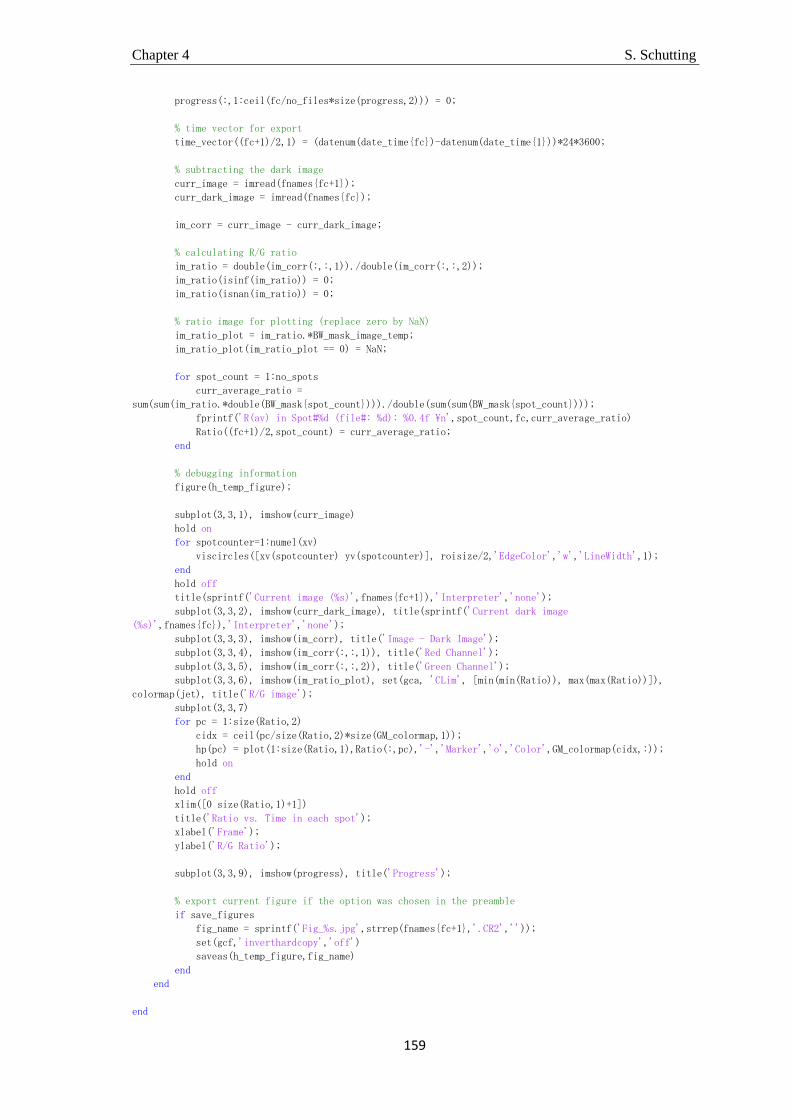
Chapter 4 S. Schutting
159
progress(:,1:ceil(fc/no_files*size(progress,2))) = 0;
% time vector for export
time_vector((fc+1)/2,1) = (datenum(date_time{fc})-datenum(date_time{1}))*24*3600;
% subtracting the dark image
curr_image = imread(fnames{fc+1});
curr_dark_image = imread(fnames{fc});
im_corr = curr_image - curr_dark_image;
% calculating R/G ratio
im_ratio = double(im_corr(:,:,1))./double(im_corr(:,:,2));
im_ratio(isinf(im_ratio)) = 0;
im_ratio(isnan(im_ratio)) = 0;
% ratio image for plotting (replace zero by NaN)
im_ratio_plot = im_ratio.*BW_mask_image_temp;
im_ratio_plot(im_ratio_plot == 0) = NaN;
for spot_count = 1:no_spots
curr_average_ratio =
sum(sum(im_ratio.*double(BW_mask{spot_count})))./double(sum(sum(BW_mask{spot_count})));
fprintf('R(av) in Spot#%d (file#: %d): %0.4f \n',spot_count,fc,curr_average_ratio)
Ratio((fc+1)/2,spot_count) = curr_average_ratio;
end
% debugging information
figure(h_temp_figure);
subplot(3,3,1), imshow(curr_image)
hold on
for spotcounter=1:numel(xv)
viscircles([xv(spotcounter) yv(spotcounter)], roisize/2,'EdgeColor','w','LineWidth',1);
end
hold off
title(sprintf('Current image (%s)',fnames{fc+1}),'Interpreter','none');
subplot(3,3,2), imshow(curr_dark_image), title(sprintf('Current dark image
(%s)',fnames{fc}),'Interpreter','none');
subplot(3,3,3), imshow(im_corr), title('Image - Dark Image');
subplot(3,3,4), imshow(im_corr(:,:,1)), title('Red Channel');
subplot(3,3,5), imshow(im_corr(:,:,2)), title('Green Channel');
subplot(3,3,6), imshow(im_ratio_plot), set(gca, 'CLim', [min(min(Ratio)), max(max(Ratio))]),
colormap(jet), title('R/G image');
subplot(3,3,7)
for pc = 1:size(Ratio,2)
cidx = ceil(pc/size(Ratio,2)*size(GM_colormap,1));
hp(pc) = plot(1:size(Ratio,1),Ratio(:,pc),'-','Marker','o','Color',GM_colormap(cidx,:));
hold on
end
hold off
xlim([0 size(Ratio,1)+1])
title('Ratio vs. Time in each spot');
xlabel('Frame');
ylabel('R/G Ratio');
subplot(3,3,9), imshow(progress), title('Progress');
% export current figure if the option was chosen in the preamble
if save_figures
fig_name = sprintf('Fig_%s.jpg',strrep(fnames{fc+1},'.CR2',''));
set(gcf,'inverthardcopy','off')
saveas(h_temp_figure,fig_name)
end
end
end

Chapter 4 S. Schutting
160
%% Genarate array containing the time vector with the respective ratios
Ratio_final = [time_vector Ratio];
%% Data and Figure export
% preallocating data of legend array
legend_array = cell(no_spots,1);
hf_plot = figure('units','normalized','outerposition',[0 0 1 1]);
% plot ratio trends vs image number in each spot
for pc = 1:no_spots
cidx = ceil(pc/size(Ratio,2)*size(GM_colormap,1));
hp(pc) = plot(1:size(Ratio,1),Ratio(:,pc),'-','Marker','o','Color',GM_colormap(cidx,:));
hold on
grid on
legend_array{pc} = sprintf('spot %d',pc);
end
hold off
title(sprintf('Ratio plot'));
legend(legend_array,'Location','EO')
saveas(gcf,sprintf('%s_Ratio_plot.pdf',datestr(datenum(date),29)))
% export data
ratio_data_filename = sprintf('%s_ratio_data.csv',datestr(datenum(date),29));
csvwrite(ratio_data_filename,Ratio_final);

Conclusion and Outlook S. Schutting
161
Conclusion and Outlook
A new pH-sensitive indicator class based on diketo-pyrrolo-pyrroles (DPPs) was
introduced (chapter 1 and 2). The new indicators were convenient to synthesize from
low-cost starting materials and feature high solubility in organic solvents and polymers,
good photostability, high quantum yields and tunable sensitivity (pKa values) due to
their substitution pattern. Even very high sensitivity was achieved by introducing
electron-donating groups. The indicators show self-referencing (dual-emitting)
absorption and fluorescence spectra in the visible range after excitation in the blue range
of the spectrum. They are usable for imaging applications after tuning their spectral
properties to meet the color channels of commercially available RGB cameras (chapter
2). The presented indicator class represents a promising alternative to state-of-the-art
indicators, e.g. HPTS.
Here, different starting materials and substituents would lead to a broader range of
possible indicator dyes. Thus, photostability and quantum yields of the deprotonated
forms could maybe improved. The DPP indicator of chapter 2 may be combined with
the multi-branched optical carbon dioxide sensor (chapter 4). The dual-emitting
properties of this dye fit perfectly to the color channels of the RGB camera and would
lead to less layers of the sensing foils (no inner-filter effect system needed) and
therefore to thinner layers and faster response times.
Furthermore, a second class of pH-sensitive indicators based on di-OH-aza-BODIPYs
was introduced (chapter 3). Using these indicators in optical carbon dioxide sensors
enables measurements in the near infrared (NIR) region, where background signals are
diminished, light scattering is low and low-cost excitation sources can be used. The
dyes feature very high and tunable pKa values (high/tunable sensitivity), excellent
photostability and absorption maxima in the NIR region. Luminescence based read-out
can be realized by making use of the inner-filter effect.
This class could also be expanded by using more different substituents. This could lead
to optimized spectral properties for low-cost materials, e.g. excitations sources (LEDs),
detectors or filters. Achieving fluorescent indicator dyes in the NIR region would enable
luminescence based read-out without needing an inner-filter effect based multi-layer

Conclusion and Outlook S. Schutting
162
system. This would combine the advantages of the NIR region with luminescence based
read-out techniques.
In the end, a multi-branched optical carbon dioxide sensor was presented, possessing
not one, but 100 freely positionable optical fibers with one collective excitation source
and imaging read-out via the color channels of an RGB camera (chapter 4). This enables
measurements with a very high spatial resolution. The applicability was demonstrated
by measuring the subsea CO2 dynamics off Panarea Island (Sicily, Italy).
Of course, this device is only a prototype and there are several improvement
possibilities: A housing made of titanium would be more stable against pressure. Hence,
the device would be applicable for deep sea measurements. As titanium is rather
expensive, the size of the device should be diminished. Thus, the spatial demands
within the housing (excitation, electronical system, camera, etc.) have to be minimized
and optimized. Data download should be enabled via cable connection to save time and
to avoid the refocusing of the camera. Up to now, the camera was fixed with only one
screw and was displaced sideways when the device was hit by greater impacts.
Therefore, the camera fixation should be extended to an (at least) two-point fixation. As
already mentioned, the combination with self-referencing and fluorescent indicator dyes
would lead to less layers of the sensing foils and therefore, to thinner and faster sensors.
Both of the presented indicator classes and the multi-branched optical carbon dioxide
sensor are promising alternatives to their respective state-of-the-art materials/devices.
Nevertheless, one should spend respect to the fact that there are still difficulties to
overcome when it comes to practical applications:
Poisoning. The pH-sensitive indicator dyes used in this thesis show changing spectral
properties according to their degree of protonation. It does not matter if the protons are
released because of the reaction mechanism with carbon dioxide or by the reaction of
e.g. weak volatile acids entering the matrix. These volatile acids can enter the protection
layer and the matrix because they are not charged. Afterwards, they dissociate and
protonate the indicator. As the remaining species are charged they can not leave the
sensor again. Hence, the indicator dye stays protonated. This so called poisoning causes
an increasing signal as consequence of an increasing degree of protonation of the

Conclusion and Outlook S. Schutting
163
indicator. In marine science H2S represents the most widespread example of a weak
volatile acid causing this problem. Protection layers for this issue are highly desired.
Adhesion of layers. As mentioned in the introduction the sensing chemistry should stick
to the support and should withstand chemical, thermal and mechanical stress. In the
majority of cases the sensing chemistry consists not only of one, but two or more layers.
The requirements for adhesion are even more difficult to meet with increasing number
of layers, especially when they display different properties concerning water uptake or
their temperature dependent expansion coefficients. For example, if a multi layer system
is exposed to altering or extreme temperatures, the single layers expand different and
thus, lose their adhesion. This makes the development of protection layers even more
complicated, but not negligible.
Stability. Sensors should feature chemical, thermal and mechanical stability. During
practical applications conditions can be harsh, long-lasting and show extreme
fluctuations.
Response time. Sensors should response fast and reversible. In marine science for
example divers are performing transect measurements, where the sensor is moved over
a certain path over the seafloor. If the sensors show too long response times these kind
of measurements are not feasible.
Cross-talks. Optical chemical sensors can measure various parameters, but this means
on the other hand that these parameters can influence the sensor. One should know the
possible influences of temperature, viscosity or electrochemical properties of the sensor
system and should plan experiments with respect to those influences.
Biofouling. If sensors are applied in marine environments, microorganisms tend to build
biofilms on the devices. Microelectrodes are less affected. When such a biofilm is built
on the sensor-sample interface, e.g. a membrane or an optode, it can falsify the
measurement results, e.g. oxygen consumption of the biofilm in front of an oxygen
sensor. Biofilms can lead to an increase of the response time, to possible cross-talks to
substances produced by the films or to poisoning of the sensor. Most widely discussed
strategies to prevent the building of biofouling are copper meshes covering the part to
be protected or silver ions. A solution for this problem is highly desired.
Conclusion and Outlook S. Schutting
164
Protection layers. The protection layers should meet several demands. They should act
as ion barrier to prevent cross-talks to the samples pH or other ionic species. Ambient
light should be excluded from the measurement. For example during sediment
measurements light scattering caused by the sediment can occur. This can change the
signal ratio and thus, the measurement results. Ideally, protection layers should stop
species like H2S (see above). They should be as thin as possible (response times!), but
stable against mechanical stress – ideally, even more as the layers below. They should
withstand scratching or impacts as e.g. in case of measurements in the sediment.
Additionally, they should feature good adhesion to the layer below and/or to the
support, similar expansion coefficients and similar water uptake. If the protection layer
is prepared with organic solvents, one has to pay attention that those are not dissolving
the upper part of the covered layer. Additionally, the indicator dye – if not covalently
coupled - should not be forced to migrate into the protection layer.
Protection layers are a significant part of optical sensing systems. Hence, one should not
underestimate the importance of this part of the sensor and should investigate great care
into the development.

References S. Schutting
165
References
(1) Falkowski, P.; Scholes, R. J.; Boyle, E.; Canadell, J.; Canfield, D.; Elser, J.; Gruber, N.;
Hibbard, K.; Hogberg, P.; Linder, S.; Mackenzie, F. T.; Moore, B.; Pedersen, T.; Rosenthal,
Y.; Seitzinger, S.; Smetacek, V.; Steffen, W. Science 2000, 290 (5490), 291–296.
(2) Post, W.; Peng, T.; Emanuel, W.; King, A.; Dale, V.; Deangelis, D. Am. Sci. 1990, 78 (4),
310–326.
(3) Baar, H. J. W. de; Stoll, M. H. C. In Climate and Energy: The Feasibility of Controlling CO2
Emissions; Okken, P. A., Swart, R. J., Zwerver, S., Eds.; Springer Netherlands, 1989; pp
143–177.
(4) Change, I. P. on C. Climate Change 2007 - The Physical Science Basis: Working Group I
Contribution to the Fourth Assessment Report of the IPCC; Cambridge University Press,
2007.
(5) Hall-Spencer, J. M.; Rodolfo-Metalpa, R.; Martin, S.; Ransome, E.; Fine, M.; Turner, S.
M.; Rowley, S. J.; Tedesco, D.; Buia, M.-C. Nature 2008, 454 (7200), 96–99.
(6) Schlesinger, W. H.; Andrews, J. A. Biogeochemistry 2000, 48 (1), 7–20.
(7) Field, C. B.; Raupach, M. R.; MacKenzie, S. H. The Global Carbon Cycle: Integrating
Humans, Climate, and the Natural World, New.; Island Pr: Washington, 2004.
(8) Fischer, null; Wahlen, null; Smith, null; Mastroianni, null; Deck, null. Science 1999,
283 (5408), 1712–1714.
(9) Fabry, V. J.; Seibel, B. A.; Feely, R. A.; Orr, J. C. Ices J. Mar. Sci. 2008, 65 (3), 414–432.
(10) Cramer, W.; Bondeau, A.; Schaphoff, S.; Lucht, W.; Smith, B.; Sitch, S. Philos. Trans. R.
Soc. Lond. Ser. B-Biol. Sci. 2004, 359 (1443), 331–343.
(11) Dickinson, R. E.; Cicerone, R. J. Nature 1986, 319 (6049), 109–115.
(12) Juntueng, S.; Towprayoon, S.; Chiarakorn, S. Resour. Conserv. Recycl. 2014, 87, 46–56.
(13) Sabine, C. L.; Feely, R. A.; Gruber, N.; Key, R. M.; Lee, K.; Bullister, J. L.; Wanninkhof, R.;
Wong, C. S.; Wallace, D. W. R.; Tilbrook, B.; Millero, F. J.; Peng, T. H.; Kozyr, A.; Ono, T.;
Rios, A. F. Science 2004, 305 (5682), 367–371.
(14) Riebesell, U.; Fabry, V. J.; Hansson, L.; Gattuso, J.-P. Guide to best practices for ocean
acidification research and data reporting; Luxembourg: Publications Office of the
European Union, 2011.
(15) Zeebe, R. E.; Wolf-Gladrow, D. CO2 in Seawater: Equilibrium, Kinetics, Isotopes:
Equilibrium, Kinetics, Isotopes; Elsevier, 2001.
(16) Dickson, A. G.; Sabine, C. L.; Christian, J. R. Guide to Best Practices for Ocean CO2
measurements; PICES Special Publication 3, 2007.
References S. Schutting
166
(17) Salmon, K. H.; Anand, P.; Sexton, P. F.; Conte, M. Biogeosciences 2015, 12 (1), 223–235.
(18) Schiebel, R. Glob. Biogeochem. Cycles 2002, 16 (4), 1065.
(19) Kara, A. B.; Rochford, P. A.; Hurlburt, H. E. J. Geophys. Res. Oceans 2000, 105 (C7),
16803–16821.
(20) Sugimura, Y.; Suzuki, Y. Mar. Chem. 1988, 24 (2), 105–131.
(21) Cripps, I. L.; Munday, P. L.; McCormick, M. I. Plos One 2011, 6 (7), e22736.
(22) Caldeira, K.; Wickett, M. E. J. Geophys. Res. Oceans 2005, 110 (C9), C09S04.
(23) Cox, P. M.; Betts, R. A.; Jones, C. D.; Spall, S. A.; Totterdell, I. J. Nature 2000, 408 (6809),
184–187.
(24) Rayner, P. J.; Stavert, A.; Scholze, M.; Ahlström, A.; Allison, C. E.; Law, R. M.
Biogeosciences 2015, 12 (3), 835–844.
(25) Pettit, E. C.; Lee, K. M.; Brann, J. P.; Nystuen, J. A.; Wilson, P. S.; O’Neel, S. Geophys. Res.
Lett. 2015, 42 (7), 2309–2316.
(26) Jeppesen, E.; Brucet, S.; Naselli-Flores, L.; Papastergiadou, E.; Stefanidis, K.; Noges, T.;
Noges, P.; Attayde, J. L.; Zohary, T.; Coppens, J.; Bucak, T.; Menezes, R. F.; Sousa Freitas,
F. R.; Kernan, M.; Sondergaard, M.; Beklioglu, M. Hydrobiologia 2015, 750 (1), 201–227.
(27) Moss, B.; Kosten, S.; Meerhoff, M.; Battarbee, R. W.; Jeppesen, E.; Mazzeo, N.; Havens,
K.; Lacerot, G.; Liu, Z.; De Meester, L.; Paerl, H.; Scheffer, M. Inland Waters 2011, 1 (2),
101–105.
(28) De Silva, C. S.; Weatherhead, E. K.; Knox, J. W.; Rodriguez-Diaz, J. A. Agric. Water
Manag. 2007, 93 (1-2), 19–29.
(29) Widdicombe, S.; Spicer, J. I. J. Exp. Mar. Biol. Ecol. 2008, 366 (1–2), 187–197.
(30) Lapennas, G. N. Respir. Physiol. 1983, 54 (2), 161–172.
(31) Dixson, D. L.; Munday, P. L.; Jones, G. P. Ecol. Lett. 2010, 13 (1), 68–75.
(32) Jutfelt, F.; Hedgaerde, M. Front. Zool. 2013, 10, 81.
(33) Wyatt, N. J.; Kitidis, V.; Woodward, E. M. S.; Rees, A. P.; Widdicombe, S.; Lohan, M. J.
Plankton Res. 2010, 32 (5), 631–641.
(34) Hassenrueck, C.; Hofmann, L. C.; Bischof, K.; Ramette, A. Environ. Microbiol. Rep. 2015,
7 (3), 516–525.
(35) Ow, Y. X.; Collier, C. J.; Uthicke, S. Mar. Biol. 2015, 162 (5), 1005–1017.
(36) Valeur, P. D. B. Molecular Fluorescence: Principles and Applications; 2001.

References S. Schutting
167
(37) Wolfbeis, O. S. Anal. Chem. 2006, 78 (12), 3859–3874.
(38) McDonagh, C.; Burke, C. S.; MacCraith, B. D. Chem. Rev. 2008, 108 (2), 400–422.
(39) Wolfbeis, O. S. J. Mater. Chem. 2005, 15 (27-28), 2657–2669.
(40) Mistlberger, G.; Crespo, G. A.; Bakker, E. Annu. Rev. Anal. Chem. Vol 7 2014, 7, 483–512.
(41) Xie, X.; Pawlak, M.; Tercier-Waeber, M.-L.; Bakker, E. Anal. Chem. 2012, 84 (7), 3163–
3169.
(42) Borisov, S. M.; Wuerth, C.; Resch-Genger, U.; Klimant, I. Anal. Chem. 2013, 85 (19),
9371–9377.
(43) Fukano, H.; Hashimoto, T.; Taue, S. Jpn. J. Appl. Phys. 2014, 53 (4), 04EG05.
(44) Takeo, T.; Hattori, H. Jpn. J. Appl. Phys. Part 1-Regul. Pap. Short Notes Rev. Pap. 1982,
21 (10), 1509–1512.
(45) Pattnaik, P. Appl. Biochem. Biotechnol. 2005, 126 (2), 79–92.
(46) Ciprian, D.; Hlubina, P. Opt. Sens. Detect. Ii 2012, 8439, 843927.
(47) Singh, S.; Gupta, B. D. Meas. Sci. Technol. 2010, 21 (11), 115202.
(48) Healey, P. J. Light. Technol. 1985, 3 (4), 876–886.
(49) Mills, A.; Hodgen, S. Adv. Concepts Fluoresc. Spectrosc. Pt Small Mol. Sens. 2005, 9, 119–
161.
(50) Mills, A.; Chang, Q. Analyst 1993, 118 (7), 839–843.
(51) Mills, A.; Chang, Q.; Mcmurray, N. Anal. Chem. 1992, 64 (13), 1383–1389.
(52) Aigner, D.; Freunberger, S. A.; Wilkening, M.; Saf, R.; Borisov, S. M.; Klimant, I. Anal.
Chem. 2014, 86 (18), 9293–9300.
(53) Aigner, D.; Borisov, S. M.; Orriach Fernandez, F. J.; Fernandez Sanchez, J. F.; Saf, R.;
Klimant, I. Talanta 2012, 99, 194–201.
(54) Gareis, T.; Huber, C.; Wolfbeis, O. S.; Daub, J. Chem. Commun. 1997, No. 18, 1717–1718.
(55) de Silva, A. P.; Gunaratne, H. Q. N.; Gunnlaugsson, T.; Huxley, A. J. M.; McCoy, C. P.;
Rademacher, J. T.; Rice, T. E. Chem. Rev. 1997, 97 (5), 1515–1566.
(56) Zaggout, F. R.; El-Nahhal, I. M.; Qaraman, A. E.-F. A.; Dahoudi, N. Al. Mater. Lett. 2006,
60 (29-30), 3463–3467.
(57) Mills, A.; Chang, Q. Anal. Chim. Acta 1994, 285 (1-2), 113–123.
(58) Chierici, M.; Fransson, A.; Anderson, L. G. Mar. Chem. 1999, 65 (3-4), 281–290.

References S. Schutting
168
(59) Peterson, J. I.; Goldstein, S. R.; Fitzgerald, R. V.; Buckhold, D. K. Anal. Chem. 1980, 52 (6),
864–869.
(60) Zaggout, F. R. Mater. Lett. 2006, 60 (8), 1026–1030.
(61) Mills, A.; Lepre, A.; Wild, L. Sens. Actuators B-Chem. 1997, 39 (1-3), 419–425.
(62) Weidgans, B. M.; Krause, C.; Klimant, I.; Wolfbeis, O. S. Analyst 2004, 129 (7), 645–650.
(63) Vasylevska, A. S.; Karasyov, A. A.; Borisov, S. M.; Krause, C. Anal. Bioanal. Chem. 2007,
387 (6), 2131–2141.
(64) Choi, M. F. J. Photochem. Photobiol. -Chem. 1997, 104 (1-3), 207–212.
(65) Bultzingslowen, C. von; McEvoy, A. K.; McDonagh, C.; MacCraith, B. D.; Klimant, I.;
Krause, C.; Wolfbeis, O. S. Analyst 2002, 127 (11), 1478–1483.
(66) Oter, O.; Ertekin, K.; Derinkuyu, S. Talanta 2008, 76 (3), 557–563.
(67) Kermis, H. R.; Kostov, Y.; Harms, P.; Rao, G. Biotechnol. Prog. 2002, 18 (5), 1047–1053.
(68) Borisov, S. M.; Gatterer, K.; Klimant, I. Analyst 2010, 135 (7), 1711–1717.
(69) Briggs, M. S.; Burns, D. D.; Cooper, M. E.; Gregory, S. J. Chem. Commun. 2000, No. 23,
2323–2324.
(70) Cooper, M. E.; Gregory, S.; Adie, E.; Kalinka, S. J. Fluoresc. 2002, 12 (3-4), 425–429.
(71) Jokic, T.; Borisov, S. M.; Saf, R.; Nielsen, D. A.; Kühl, M.; Klimant, I. Anal. Chem. 2012, 84
(15), 6723–6730.
(72) Cajlakovic, M.; Suppan, M.; Pressler, H.; Ribitsch, V.; Bellouard, F.; Rault, S. 2011 Fifth
Int. Conf. Sens. Technol. ICST 2011 2011, 411–416.
(73) Antala, D. K.; Varshney, A. K.; Davara, P. R.; Sangani, V. P. Packag. Technol. Sci. 2015, 28
(6), 557–564.
(74) Rai, D. R.; Oberoi, H. S.; Baboo, B. J. Food Sci. Technol.-Mysore 2002, 39 (3), 199–207.
(75) Del Valle Rodriguez Castilla, M.; Jordano, R. Alimentaria 1997, 35 (285), 79–99.
(76) Stow, R. W.; Baer, R. F.; Randall, B. F. Arch. Phys. Med. Rehabil. 1957, 38 (10), 646–650.
(77) Severinghaus, J. W.; Bradley, A. F. J. Appl. Physiol. 1958, 13 (3), 515–520.
(78) Nunn, J. F. Proc. R. Soc. Med. 1960, 53 (3), 180–182.
(79) Suzuki, H.; Arakawa, H.; Sasaki, S.; Karube, I. Anal. Chem. 1999, 71 (9), 1737–1743.
(80) Hesse, M.; Meier, H.; Zeeh, B. Spektroskopische Methoden in der organischen Chemie,
7., überarb. A.; Thieme, Stuttgart, 2005.

References S. Schutting
169
(81) Wang, X.-D.; Wolfbeis, O. S. Anal. Chem. 2013, 85 (2), 487–508.
(82) E Farish, S. J. Anesth. Clin. Res. 2013, 04 (03).
(83) Park, C. S.; Kwak, J. G.; Lee, C.; Lee, C.-H.; Lee, S. K.; Kim, Y. L. Perfus.-Uk 2011, 26 (6),
524–528.
(84) Zhi-hua, T.; Yang, Z.; Li-wen, Z.; Guo-dong, J.; Li-hua, C.; Xin-xiao, Y. Spectrosc. Spectr.
Anal. 2015, 35 (4), 997–1000.
(85) Clegg, M.; Sullivan, C.; Eastin, J. Plant Physiol. 1978, 62 (6), 924–926.
(86) Arieli, R.; Ertracht, O.; Daskalovic, Y. J. Appl. Physiol. 1999, 86 (2), 647–650.
(87) Degrandpre, M.; Hammar, T.; Smith, S.; Sayles, F. Limnol. Oceanogr. 1995, 40 (5), 969–
975.
(88) Lefevre, N.; Ciabrini, J.; Michard, G.; Brient, B.; Duchaffaut, M.; Merlivat, L. Mar. Chem.
1993, 42 (3-4), 189–198.
(89) Mills, A.; Monaf, L. Analyst 1996, 121 (4), 535–540.
(90) Ekeberg, D.; Ogner, G.; Fongen, M.; Joner, E. J.; Wickstrøm, T. J. Environ. Monit. 2004, 6
(7), 621–623.
(91) Fietzek, P.; Fiedler, B.; Steinhoff, T.; Koertzinger, A. J. Atmospheric Ocean. Technol.
2014, 31 (1), 181–196.
(92) Weigl, B.; Holobar, A.; Trettnak, W.; Klimant, I.; Kraus, H.; Oleary, P.; Wolfbeis, O. J.
Biotechnol. 1994, 32 (2), 127–138.
(93) Beuermann, T.; Egly, D.; Geoerg, D.; Klug, K. I.; Storhas, W.; Methner, F.-J. J. Biosci.
Bioeng. 2012, 113 (3), 399–405.
(94) Murray, I. P.; Modell, J. H. Anesthesiology 1983, 59 (4), 344–346.
(95) Rost, B.; Zondervan, I.; WolfGladrow, D. Mar. Ecol. Prog. Ser. 2008, 373, 227–237.
(96) Fabricius, K. E.; Langdon, C.; Uthicke, S.; Humphrey, C.; Noonan, S.; ath, G. De’; Okazaki,
R.; Muehllehner, N.; Glas, M. S.; Lough, J. M. Nat. Clim. Change 2011, 1 (3), 165–169.
(97) Orr, J. C.; Fabry, V. J.; Aumont, O.; Bopp, L.; Doney, S. C.; Feely, R. A.; Gnanadesikan, A.;
Gruber, N.; Ishida, A.; Joos, F.; Key, R. M.; Lindsay, K.; Maier-Reimer, E.; Matear, R.;
Monfray, P.; Mouchet, A.; Najjar, R. G.; Plattner, G.-K.; Rodgers, K. B.; Sabine, C. L.;
Sarmiento, J. L.; Schlitzer, R.; Slater, R. D.; Totterdell, I. J.; Weirig, M.-F.; Yamanaka, Y.;
Yool, A. Nature 2005, 437 (7059), 681–686.
(98) Doney, S. C.; Fabry, V. J.; Feely, R. A.; Kleypas, J. A. In Annual Review of Marine Science;
Annual Reviews: Palo Alto, 2009; Vol. 1, pp 169–192.
(99) Puligundla, P.; Jung, J.; Ko, S. Food Control 2012, 25 (1), 328–333.

References S. Schutting
170
(100) Oter, O.; Ertekin, K.; Topkaya, D.; Alp, S. Sens. Actuators B-Chem. 2006, 117 (1), 295–
301.
(101) Nakamura, N.; Amao, Y. Sens. Actuators B-Chem. 2003, 92 (1-2), 98–101.
(102) Perez de Vargas-Sansalvador, I. M.; Carvajal, M. A.; Roldan-Munoz, O. M.; Banqueri, J.;
Fernandez-Ramos, M. D.; Capitan-Vallvey, L. F. Anal. Chim. Acta 2009, 655 (1-2), 66–74.
(103) Perez de Vargas-Sansalvador, I. M.; Martinez-Olmos, A.; Palma, A. J.; Dolores
Fernandez-Ramos, M.; Fermin Capitan-Vallvey, L. Microchim. Acta 2011, 172 (3-4), 455–
464.
(104) Ali, R.; Saleh, S. M.; Meier, R. J.; Azab, H. A.; Abdelgawad, I. I.; Wolfbeis, O. S. Sens.
Actuators B Chem. 2010, 150 (1), 126–131.
(105) Neurauter, G.; Klimant, I.; Wolfbeis, O. S. Anal. Chim. Acta 1999, 382 (1-2), 67–75.
(106) Bultzingslowen, C. von; McEvoy, A. K.; McDonagh, C.; MacCraith, B. D. Anal. Chim. Acta
2003, 480 (2), 275–283.
(107) Marazuela, M. D.; Moreno-Bondi, M. C.; Orellana, G. Appl. Spectrosc. 1998, 52 (10),
1314–1320.
(108) Schulman, S.; Chen, S.; Bai, F.; Leiner, M.; Weis, L.; Wolfbeis, O. Anal. Chim. Acta 1995,
304 (2), 165–170.
(109) Wolfbeis, O.; Weis, L.; Leiner, M.; Ziegler, W. Anal. Chem. 1988, 60 (19), 2028–2030.
(110) Spry, D. B.; Goun, A.; Fayer, M. D. J. Phys. Chem. A 2007, 111 (2), 230–237.
(111) Wolfbeis, O. S.; Kovács, B.; Goswami, K.; Klainer, S. M. Microchim. Acta 1998, 129 (3),
181–188.
(112) Borisov, S. M.; Krause, C.; Arain, S.; Wolfbeis, O. S. Adv. Mater. 2006, 18 (12), 1511–
1516.
(113) Dansby-Sparks, R. N.; Jin, J.; Mechery, S. J.; Sampathkumaran, U.; Owen, T. W.; Yu, B. D.;
Goswami, K.; Hong, K.; Grant, J.; Xue, Z.-L. Anal. Chem. 2010, 82 (2), 593–600.
(114) Zhujun, Z.; Seitz, W. R. Anal. Chim. Acta 1984, 160 (0), 305–309.
(115) Haugland, R. P. The Molecular Probes Handbook - A guide to Fluorescent Probes and
Labeling Technologies, Tenth Edition.; Invitrogen Corp.: USA, 2005.
(116) Pandey, S.; Baker, S. N.; Pandey, S.; Baker, G. A. Chem. Commun. 2012, 48 (56), 7043–
7045.
(117) Liu, Y.; Tang, Y.; Barashkov, N. N.; Irgibaeva, I. S.; Lam, J. W. Y.; Hu, R.; Birimzhanova, D.;
Yu, Y.; Tang, B. Z. J. Am. Chem. Soc. 2010, 132 (40), 13951–13953.
References S. Schutting
171
(118) Ali, R.; Lang, T.; Saleh, S. M.; Meier, R. J.; Wolfbeis, O. S. Anal. Chem. 2011, 83 (8), 2846–
2851.
(119) Zollinger, H. Color Chemistry: Syntheses, Properties, and Applications of Organic Dyes
and Pigments; John Wiley & Sons, 2003.
(120) Luňák Jr., S.; Vala, M.; Vyňuchal, J.; Ouzzane, I.; Horáková, P.; Možíšková, P.; Eliáš, Z.;
Weiter, M. Dyes Pigments 2011, 91 (3), 269–278.
(121) Wang, B.; He, N.; Li, B.; Jiang, S.; Qu, Y.; Qu, S.; Hua, J. Aust. J. Chem. 2012, 65 (4), 387–
394.
(122) Zhu, Y.; Rabindranath, A. R.; Beyerlein, T.; Tieke, B. Macromolecules 2007, 40 (19),
6981–6989.
(123) Cao, D. R.; Liu, Q. L.; Zeng, W. J.; Han, S. H.; Peng, J. B.; Liu, S. P. J. Polym. Sci. Part -
Polym. Chem. 2006, 44 (8), 2395–2405.
(124) Rabindranath, A. R.; Zhu, Y.; Heim, I.; Tieke, B. Macromolecules 2006, 39 (24), 8250–
8256.
(125) Zhu, Y.; Heim, I.; Tieke, B. Macromol. Chem. Phys. 2006, 207 (23), 2206–2214.
(126) Zhang, X.; Richter, L. J.; DeLongchamp, D. M.; Kline, R. J.; Hammond, M. R.; McCulloch,
I.; Heeney, M.; Ashraf, R. S.; Smith, J. N.; Anthopoulos, T. D.; Schroeder, B.; Geerts, Y. H.;
Fischer, D. A.; Toney, M. F. J. Am. Chem. Soc. 2011, 133 (38), 15073–15084.
(127) Qu, Y.; Hua, J.; Tian, H. Org. Lett. 2010, 12 (15), 3320–3323.
(128) Jeong, Y.-H.; Lee, C.-H.; Jang, W.-D. Chem.- Asian J. 2012, 7 (7), 1562–1566.
(129) Demas, J.; Crosby, G. J. Phys. Chem. 1971, 75 (8), 991 – &.
(130) Seybold, G.; Wagenblast, G. Dyes Pigments 1989, 11 (4), 303–317.
(131) Ford, W. J. Photochem. 1987, 37 (1), 189–204.
(132) Borisov, S. M.; Seifner, R.; Klimant, I. Anal. Bioanal. Chem. 2011, 400 (8), 2463–2474.
(133) Vala, M.; Vynuchal, J.; Toman, P.; Weiter, M.; Lunak, S. Dyes Pigments 2010, 84 (2),
176–182.
(134) Vala, M.; Weiter, M.; Vynuchal, J.; Toman, P.; Lunak, S. J. Fluoresc. 2008, 18 (6), 1181–
1186.
(135) Hansch, C.; Leo, A.; Taft, R. W. Chem. Rev. 1991, 91 (2), 165–195.
(136) Lunak, S.; Vynuchal, J.; Vala, M.; Havel, L.; Hrdina, R. Dyes Pigments 2009, 82 (2), 102–
108.
(137) Apostolidis, A. Combinatorial Approach for Development of Optical Gas Sensors -
Concept and Application of High-Throughput Experimentation, Universität Regensburg:
References S. Schutting
172
Regensburg, 2004.
(138) Rost, B.; Zondervan, I.; Wolf-Gladrow, D. Mar. Ecol. Prog. Ser. 2008, 373, 227–237.
(139) García-Fresnadillo, D.; Marazuela, M. D.; Moreno-Bondi, M. C.; Orellana, G. Langmuir
1999, 15 (19), 6451–6459.
(140) Hong, W.; Chen, Y.; Feng, X.; Yan, Y.; Hu, X.; Zhao, B.; Zhang, F.; Zhang, D.; Xu, Z.; Lai, Y.
Chem. Commun. 2013, 49 (74), 8229–8231.
(141) Mayr, T.; Klimant, I.; Wolfbeis, O. S.; Werner, T. Anal. Chim. Acta 2002, 462 (1), 1–10.
(142) Huber, C.; Klimant, I.; Krause, C.; Wolfbeis, O. S. Anal. Chem. 2001, 73 (9), 2097–2103.
(143) Liebsch, G.; Klimant, I.; Krause, C.; Wolfbeis, O. S. Anal. Chem. 2001, 73 (17), 4354–
4363.
(144) Xu, Z.; Rollins, A.; Alcala, R.; Marchant, R. E. J. Biomed. Mater. Res. 1998, 39 (1), 9–15.
(145) Hunter, R. C.; Beveridge, T. J. Appl. Environ. Microbiol. 2005, 71 (5), 2501–2510.
(146) Spitzer, K. W.; Skolnick, R. L.; Peercy, B. E.; Keener, J. P.; Vaughan-Jones, R. D. J. Physiol.
2002, 541 (1), 159–167.
(147) Ramshesh, V. K.; Lemasters, J. J. In Mitochondrial Bioenergetics: Methods and Protocols;
Palmeira, C. M., Moreno, A. J., Eds.; 2012; Vol. 810, pp 243–248.
(148) Liebsch, G.; Klimant, I.; Frank, B.; Holst, G.; Wolfbeis, O. S. Appl. Spectrosc. 2000, 54 (4),
548–559.
(149) Wang, X.; Meier, R. J.; Wolfbeis, O. S. Angew. Chem. Int. Ed. 2013, 52 (1), 406–409.
(150) Schreml, S.; Meier, R. J.; Wolfbeis, O. S.; Landthaler, M.; Szeimies, R.-M.; Babilas, P.
Proc. Natl. Acad. Sci. U. S. A. 2011, 108 (6), 2432–2437.
(151) Peng, H.; Stolwijk, J. A.; Sun, L.-N.; Wegener, J.; Wolfbeis, O. S. Angew. Chem.-Int. Ed.
2010, 49 (25), 4246–4249.
(152) Aigner, D.; Ungerboeck, B.; Mayr, T.; Saf, R.; Klimant, I.; Borisov, S. M. J. Mater. Chem. C
2013, 1 (36), 5685–5693.
(153) Wang, X.; Meier, R. J.; Link, M.; Wolfbeis, O. S. Angew. Chem. Int. Ed. 2010, 49 (29),
4907–4909.
(154) Kondrashina, A.; Dmitriev, R.; Borisov, S. M.; Klimant, I.; O´Brien, I.; Nolan, Y. M.;
Zhdanov, A.; Papkovsky, D. Adv. Funtional Mater. 22, 4931–4939.
(155) Larsen, M.; Borisov, S. M.; Grunwald, B.; Klimant, I.; Glud, R. N. Limnol. Oceanogr.-
Methods 2011, 9, 348–360.

References S. Schutting
173
(156) Staal, M.; Borisov, S. M.; Rickelt, L. F.; Klimant, I.; Kuhl, M. J. Microbiol. Methods 2011,
85 (1), 67–74.
(157) Schutting, S.; Borisov, S. M.; Klimant, I. Anal. Chem. 2013, 85 (6), 3271–3279.
(158) Wong, W. W. H.; Subbiah, J.; Puniredd, S. R.; Purushothaman, B.; Pisula, W.; Kirby, N.;
Müllen, K.; Jones, D. J.; Holmes, A. B. J. Mater. Chem. 2012, 22 (39), 21131–21137.
(159) Qu, S.; Wu, W.; Hua, J.; Kong, C.; Long, Y.; Tian, H. J. Phys. Chem. C 2010, 114 (2), 1343–
1349.
(160) Qu, S.; Tian, H. Chem. Commun. 2012, 48 (25), 3039–3051.
(161) Langhals, H.; Potrawa, T.; Nöth, H.; Linti, G. Angew. Chem. Int. Ed. Engl. 1989, 28 (4),
478–480.
(162) Langhals, H.; Grundei, T.; Potrawa, T.; Polborn, K. Liebigs Ann. 1996, 1996 (5), 679–682.
(163) Lorenz, I.-P.; Limmert, M.; Mayer, P.; Piotrowski, H.; Langhals, H.; Poppe, M.; Polborn, K.
Chem. – Eur. J. 2002, 8 (17), 4047–4055.
(164) Langhals, H.; Limmert, M.; Lorenz, I.-P.; Mayer, P.; Piotrowski, H.; Polborn, K. Eur. J.
Inorg. Chem. 2000, 2000 (11), 2345–2349.
(165) Yamagata, T.; Kuwabara, J.; Kanbara, T. Tetrahedron Lett. 2010, 51 (12), 1596–1599.
(166) Lebourgeois, V.; Bégué, A.; Labbé, S.; Mallavan, B.; Prévot, L.; Roux, B. Sensors 2008, 8
(11), 7300–7322.
(167) Zhao, D.; Miller, D.; Xian, X.; Tsow, F.; Forzani, E. S. Sens. Actuators B Chem. 2014, 195,
171–176.
(168) Trivedi, S.; Mehta, H.; Kashyap, R. Indian J. Crit. Care Med. 2014, 18 (6), 348.
(169) Punt, A. E.; Poljak, D.; Dalton, M. G.; Foy, R. J. Ecol. Model. 2014, 285, 39–53.
(170) Carroll, A. G.; Przeslawski, R.; Radke, L. C.; Black, J. R.; Picard, K.; Moreau, J. W.; Haese,
R. R.; Nichol, S. Cont. Shelf Res. 2014, 83, 116–128.
(171) Zosel, J.; Oelßner, W.; Decker, M.; Gerlach, G.; Guth, U. Meas. Sci. Technol. 2011, 22 (7),
072001.
(172) Xu, L. Q.; Zhang, B.; Sun, M.; Hong, L.; Neoh, K.-G.; Kang, E.-T.; Fu, G. D. J. Mater. Chem.
A 2013, 1 (4), 1207–1212.
(173) Xu, Q.; Lee, S.; Cho, Y.; Kim, M. H.; Bouffard, J.; Yoon, J. J. Am. Chem. Soc. 2013, 135
(47), 17751–17754.
(174) Borchert, N. B.; Kerry, J. P.; Papkovsky, D. B. Sens. Actuators B Chem. 2013, 176, 157–
165.

References S. Schutting
174
(175) Schutting, S.; Klimant, I.; Beer, D. de; Borisov, S. M. Methods Appl. Fluoresc. 2014, 2 (2),
024001.
(176) Borisov, S. M.; Klimant, I. Anal. Chim. Acta 2013, 787, 219–225.
(177) Nakamura, N.; Amao, Y. Anal. Bioanal. Chem. 2003, 376 (5), 642–646.
(178) Amao, Y.; Nakamura, N. Sens. Actuators B Chem. 2004, 100 (3), 347–351.
(179) Hall, M. J.; McDonnell, S. O.; Killoran, J.; O’Shea, D. F. J. Org. Chem. 2005, 70 (14), 5571–
5578.
(180) Gorman, A.; Killoran, J.; O’Shea, C.; Kenna, T.; Gallagher, W. M.; O’Shea, D. F. J. Am.
Chem. Soc. 2004, 126 (34), 10619–10631.
(181) Oliver, A. E.; Newbold, L. K.; Whiteley, A. S.; van der Gast, C. J. Environ. Microbiol. Rep.
2014, 6 (6), 574–582.
(182) Pedersen, S. A.; Vage, V. T.; Olsen, A. J.; Hammer, K. M.; Altin, D. J. Toxicol. Environ.
Health-Part -Curr. Issues 2014, 77 (9-11), 535–549.
(183) Hutchins, D. A.; Fu, F.-X.; Webb, E. A.; Walworth, N.; Tagliabue, A. Nat. Geosci. 2013, 6
(9), 790–795.
(184) Iguchi, A.; Kumagai, N. H.; Nakamura, T.; Suzuki, A.; Sakai, K.; Nojiri, Y. Mar. Pollut. Bull.
2014, 89 (1-2), 348–355.
(185) Heuer, R. M.; Grosell, M. Am. J. Physiol.-Regul. Integr. Comp. Physiol. 2014, 307 (9),
R1061–R1084.
(186) Green, L.; Jutfelt, F. Biol. Lett. 2014, 10 (9), 20140538.
(187) Wencel, D.; Abel, T.; McDonagh, C. Anal. Chem. 2014, 86 (1), 15–29.
(188) Aigner, D.; Borisov, S. M.; Klimant, I. Anal. Bioanal. Chem. 2011, 400 (8), 2475–2485.
(189) Zhujun, Z.; Seitz, W. Anal. Chim. Acta 1984, 160 (JUN), 47–55.
(190) Hecht, H.; Kolling, A. Sens. Actuators B-Chem. 2001, 81 (1), 76–82.
(191) Stich, M. I. J.; Borisov, S. M.; Henne, U.; Schaeferling, M. Sens. Actuators B-Chem. 2009,
139 (1), 204–207.
(192) Stahl, H.; Warnken, K. W.; Sochaczewski, L.; Glud, R. N.; Davison, W.; Zhang, H. Limnol.
Oceanogr. Methods 2012, 10, 389–401.
(193) Lippitsch, M.; Pusterhofer, J.; Leiner, M.; Wolfbeis, O. Anal. Chim. Acta 1988, 205 (1-2),
1–6.
(194) Muller, B.; Hauser, P. C. Analyst 1996, 121 (3), 339–343.

References S. Schutting
175
(195) Preininger, C.; Klimant, I.; Wolfbeis, O. S. Anal. Chem. 1994, 66 (11), 1841–1846.
(196) Klimant, I.; Meyer, V.; Kuhl, M. Limnol. Oceanogr. 1995, 40 (6), 1159–1165.
(197) Warner, M. Anal. Chem. 1986, 58 (7), A766 – &.
(198) Jordan, D. M.; Walt, D. R.; Milanovich, F. P. Anal. Chem. 1987, 59 (3), 437–439.
(199) Holst, G.; Glud, R. N.; Kühl, M.; Klimant, I. Sens. Actuators B Chem. 1997, 38 (1–3), 122–
129.
(200) Yi, Z.; Zhong, Z.; Reardon, K. F.; Wang, W.; Katragadda, M.; Lear, K. L. Proc. SPIE - Int.
Soc. Opt. Eng. 2010, 7559, 75590T (6 pp.).
(201) Fischer, J. P.; Koop-Jakobsen, K. Sens. Actuators B Chem. 2012, 168, 354–359.

References S. Schutting
176
Appendix S. Schutting
177
Appendix A
List of Figures
Figure I. Global carbon cycle. 3 Figure II. Reactions of carbon dioxide in water. 5 Figure III. Scheme of the responsible biological processes. 6 Figure IV. Influencing processes on DIC and total alkalinity. 15 Figure V. Scheme of ground state, singlet excited state and triplet-excited state. 16 Figure VI . Perrin-Jablonski diagram. 18 Figure VII . Scheme of photoinduced proton transfer (PPT). 26 Figure VIII . Scheme of photoinduced electron transfer (PET). 27 Figure IX . Scheme of the inner-filter-effect. 28 Figure X. Scheme of sensor with/without protection layer. 30 Figure XI. HydroC device from Contros (Picture from CONTROS). 35 Figure XII. The GasPro - Dissolved CO2 probe. 37 Figure XIII. Optical chemical sensors. 39 Figure XIV. The Severinghaus CO2 sensor. 41 Figure 1.1. Watersoluble DPP - pKa determination. 60 Figure 1.2. Abs and em spectra of DPP dye 2. 62 Figure 1.3. Photographic images of the planar optode. 63 Figure 1.4. Calibration curves for the sensors based on DPP 2-4. 66 Figure 1.5. Comparison of CO2 sensors containing HPTS and dye 2. 67 Figure 1.6. Fluorescence intensity for alternating pCO2 values. 69 Figure S1.1. Abs and em spectra for DPP dye 3 and 4. 71 Figure S1.2. Photodegradation profiles. Figure S1.3. Abs and emspectra for CO2 sensors (dye 3 and 4). 72 Figure S1.4. Abs and em spectra for different dye concentrations. Figure S1.5. Calibration curve of a sensor based on 2. 73 Figure S1.6. Calibration curve of a sensor based on 4. Figure S1.7. Temperature dependence for the CO2 sensor. 74 Figure S1.8. Em spectrum of a CO2 sensor based on HPTS(TOA)3. Figure S1.9. Fluorescence intensity for alternating pCO2. 75 Figure S1.10. Fluorescence intensity for alternating pCO2. Figure S1.11. Fluorescence intensity of HPTS(TOA)3. 76 Figure S1.12. 1H NMR spectrum of 1. Figure S1.13. 1H 1H COSY NMR spectrum of 1. 77 Figure S1.14. MALDI-TOF mass spectrum of 1. 78 Figure S1.15. 1H NMR spectrum of 2. 79 Figure S1.16. MALDI-TOF mass spectrum of 2. 80 Figure S1.17. 1H NMR spectrum of 3. 81 Figure S1.18. MALDI-TOF mass spectrum of 3. 81/82
Appendix S. Schutting
178
Figure S1.19. 1H NMR spectrum of 4. 82 Figure S1.20. MALDI-TOF mass spectrum of 4. 83 Figure 2.1. Abs and em spectra DPPtBu3 in THF. 93 Figure 2.2. Abs and em spectra of the CO2 sensor based on DPPtBu3. 95 Figure 2.3. Calibration curves of carbon dioxide sensor based on DPPtBu3. 97 Figure 2.4. Abs at alternating pCO2. 98 Figure 2.5. Photographic images of a sensor based on DPPtBu3. 99 Figure S2.1. pKa value estimation. Figure S2.2. Photodegradation profiles. 100 Figure S2.3. Abs at alternating levels of pCO2 (dry conditions). Figure S2.4. Em spectra for different dye concentrations. 101 Figure 3.1. Abs spectra and titration curves. 116 Figure 3.2. Abs spectra of CO2 sensors. 118 Figure 3.3. Calibration curves. 120 Figure 3.4. Theory of the inner-filter effect. 122 Figure 3.5. CO2 dynamics of a Hebe plant. 123 Figure S3.1. Photodegradation profiles di-OH-aza-BODIPY. 125 Figure S3.2. EI-DI MS of the di-butoxy-complex. 126 Figure S3.3. 1H NMR of the di-butoxy-complex. 127 Figure S3.4. EI-DI MS of the di-OH-complex. 128 Figure S3.5. 1H NMR of di-OH-complex. 129 Figure S3.6. DI-EI MS of the di-F-di-OH-complex. 130 Figure S3.7. 1H NMR of the di-F-di-OH-complex. 131 Figure S3.8. EI-DI MS of the di-Cl-di-OH-complex. 132 Figure S3.9. 1H NMR of the di-Cl-di-OH-complex. 133 Figure S3.10. EI-DI MS of the di-CH3-di-OH-complex. 134 Figure S3.11. 1H NMR of the di-CH3-di-OH-complex. 135 Figure 4.1. Scheme of a sensing foil. 142 Figure 4.2. Principle of the MuFO. 145 Figure 4.3. Theory of inner-filter effect. 146 Figure 4.4. Photodegradation profiles. 147 Figure 4.5. Calibration curves of the MuFO. 148 Figure 4.6. MuFO underwater. 150 Figure 4.7. Bundle positioning and CO2 dynamics at Panarea Island. 151 Figure S4.1. Calibration curves after sealing of metal sleeves. ….154

Appendix S. Schutting
179
List of Schemes
Scheme 1.1. Synthesis of DPP dyes 1 and 2 and dye 3 and 4. 59 Scheme 2.1. Synthesis of DPPtBu3. 92 Scheme 3.1. 4-step-synthesis of the di-OH-aza-BODIPY chelates. 115
List of Tables
Table I. Averaged standard chemical composition of seawater. 11 Table II. T-dependent Henry constants and CO2 concentration. 13 Table III. Characteristic times of transitions. 19 Table IV. State-of-the-art indicators for optical CO2 sensors. 29 Table V. Technical data of different CO2 sensors. 43 Table 1.1. Photophysical properties of all the DPP dyes in THF. 61 Table 1.2. Photophysical properties of all the DPP dyes in EC49. 64 Table S1.1. Elementary analysis for the DPP starting pigments. 84 Table 2.1. Comparison of the photophysical properties. 93 Table 3.1. Photophysical properties of the di-OH-aza-BODIPY dyes. 117

Appendix S. Schutting
180
Appendix B – Curriculum Vitae
Susanne Schutting
Born on December 14, 1986 (Leoben, Austria) Marital Status: unmarried Nationality: Austria
Current Address: Dr.-Theodor-Körnerstraße 23/6 8600 Bruck an der Mur Austria
Permanent Address: Mürzstraße 1 8641 St. Marein im Mürztal Austria
Practical Experience:
- Aug. 2014 to present TU Graz – Graz University of Technology (Institute of Analytical Chemistry and Food Chemistry; university assistant/PhD student)
- Aug. 2011 to Jul. 2014 TU Graz (Institute of Analytical Chemistry and Food Chemistry; project assistant/ PhD student)
- Oct. 2010 to Jul. 2011 RCPE- Research Centre Pharmaceutical Engineering (and Institute for Process and Particle Engineering; project member)
- Jul. 2010 to Sep. 2010 RCPE (trainee)
- May 2010 to Jun. 2010 TU Graz (Institute of Analytical Chemistry; undergraduate project assistant)
- Oct. 2009 to Jan. 2010 TU Graz (Institute of Analytical Chemistry; student assistant)
- Jun. 2008 to Jan. 2010 Company “4a medicom”
- Oct. 2007 to Apr. 2010 Catering Service “Ivents”
- Feb. 2005 to Jul. 2006 Catering Service “S-Events”
Educational Background:
- Aug. 2011 to present PhD studies at TU Graz (“Optical carbon dioxide sensors for marine applications”); oral examination expected in Sep./Oct. 2015

Appendix S. Schutting
181
- Oct. 2010 to Jun. 2011 Master thesis at TU Graz (“Development of zinc electrodes for rechargeable zinc-air-batteries“)
- 2009 to 2011 TU Graz, Master studies Technical Chemistry
- 2006 to 2009 TU Graz, Bachelor studies Chemistry (focus: Technical Chemistry)
- Year 2001/02 to 2005/06 HTL-Kapfenberg – College of Materials Engineering in Kapfenberg (focus: Polymer and Environmental Engineering)
Special Skills:
- Driving licence (A, B) - Languages: German (native), English (fluent), Italian (basic) - Advanced computer skills in: MS Word, MS Power Point, MS Excel, Origin,
Inkscape - Competence Training for Student Assistants: Group Management,
Communication, Teamwork and Motivation
Articles:
2015 NIR Optical Carbon Dioxide Sensors based on Highly Photostable Dihydroxy-aza-BODIPY Dyes; S. Schutting, T. Jokic, M. Strobl, S. M. Borisov, D. de Beer, I. Klimant; J. Mater. Chem. C, 2015, 3, 5474-5483
2014 New Highly Fluorescent pH Indicator for Ratiometric RGB Imaging of pCO2; S.Schutting, I. Klimant, D. de Beer, S. M. Borisov; Methods Appl. Fluoresc., 2014, 2, 1-8
2013 Diketo-Pyrrolo-Pyrrole Dyes as New Colorimetric and Fluorescent pH Indicators for Optical Carbon Dioxide Sensors; S. Schutting, S. M. Borisov, I. Klimant; Anal. Chem., 2013, 85, 3271-3279
Poster Presentations:
2015 Neuartige optische pCO2-Sensoren basierend auf BF2-Chelatverbindungen von Dihydroxy-aza-Dipyrromethenen; E. Fritzsche, S. Schutting, T. Jokic, M. Strobl, S. M. Borisov, I.Klimant; at the ANAKON conference; Graz (Austria), 23/03/2015
New High Performance Optical pCO2 Sensors based on BF2-CHelates of Dihydroxy-aza-Dipyrromethene; E. Fritzsche, S. Schutting, T. Jokic, M. Strobl, S. M. Borisov, I.Klimant; at the Aquatic Science Meeting; Granada (Spain), 23/02/2015
Appendix S. Schutting
182
2014 A Multiple Fibre Optic Device for Monitoring Carbon Dioxide in Marine Environments; S. Schutting, J. P. Fischer, S. M. Borisov, D. de Beer, I. Klimant; at the 3rd annual project meeting (ECO2 project); Salina Island (Italy), 02/06/2014
2013 Highly Fluorescent Diketo-Pyrrolo-Pyrrole Dyes for Optical pH and CO2 Sensors; S. Schutting, D. Aigner, S. M. Borisov, I. Klimant; at the Methods and Applications of Fluorescence conference; Genova (Italy), 08/09/2013
2012 Diketo-Pyrrolo-Pyrrole Dyes as New pH Indicators for Optical CO2 Sensors in Marine Research; S. Schutting, S. M. Borisov, I. Klimant; at the Europt(r)ode XI conference; Barcelona (Spain), 01/04/2012
2011 Novel Materials for Electrically Rechargeable Zinc-Air-Batteries; S. Weinberger, G. Rabenstein, V. Hacker, K. Fröhlich, F. B. Wede, D. Movrin, S. Schutting, W. Taucher-Mautner, F. Duff; at the 4th International Summer School on Advanced Studies of Polymer Electrolyte Fuel Cells; Yokohama (Japan), 05/09/2011
New Electrode Materials for the Rechargeable Zinc-Air-Battery; S. Weinberger, G. Rabenstein, V. Hacker, K. Fröhlich, F. Duff, F. B. Wede, S. Schutting, W. Taucher-Mautner, D. Movrin, P. Janewit; at the 62nd annual meeting of the International Society of Electrochemistry; Niigata (Japan), 11/09/2011
Oral Presentations:
2014 Novel BF2-Chelated Tetraarylazadipyrromethene Dyes for Optical Sensing of pH and Carbon Dioxide; S. M. Borisov, T. Jokic, M. Strobl, S. Schutting, I. Klimant; at the 8th International Conference on Porphyrins and Phthalocyanines (ICPP-8); Istanbul (Turkey), 24/06/2014
Optical Carbon Dioxide Sensors based on Novel Indicator Dyes with Outstanding Photophysical Properties; S. Schutting, T. Jokic, M. Strobl, S. M. Borisov, D. de Beer, I. Klimant; at the Europt(r)ode XII conference; Athens (Greece), 13/04/2014
2011 Development of Zinc-Electrodes for Rechargeable Zinc-Air-Batteries; S. Schutting, W. Taucher-Mautner, K. Fröhlich, S. Weinberger, V. Hacker; at the 14th Austrian Chemistry Days; Linz (Austria), 26/09/2011
Optimized Carrier Particles for Dry Powder Inhalers by the Use of Spray Drying; E. Littringer, A. Mescher, H. Schröttner, S. Schutting, P. Walzel, N. A. Urbanetz; at the 5th International Congress on Pharmaceutical Engineering; Graz (Austria), 29/09/2011