positive quaternion kähler manifolds
TRANSCRIPT
Manuel Amann
Positive Quaternion Kahler Manifolds
2009

Mathematik
Positive Quaternion Kahler Manifolds
Inaugural-Dissertationzur Erlangung des Doktorgrades
der Naturwissenschaften im FachbereichMathematik und Informatik
der Mathematisch-Naturwissenschaftlichen Fakultatder Westfalischen Wilhelms-Universitat Munster
vorgelegt vonManuel Amann
aus Bad Mergentheim
2009

Dekan: Prof. Dr. Dr. h.c. Joachim CuntzErster Gutachter: Prof. Dr. Burkhard WilkingZweiter Gutachter: Prof. Dr. Anand DessaiTag der mundlichen Prufung: 10. Juli 2009Tag der Promotion: 10. Juli 2009
Fur meine Eltern
Rita und Paul
und meinen Bruder
Benedikt

When the hurlyburly’s done,When the battle’s lost and won.
William Shakespeare, “Macbeth”

Preface
Positive Quaternion Kahler Geometry lies in the intersection of very classical yetrather different fields in mathematics. Despite its geometrical setting which involvesfundamental definitions from Riemannian geometry, it was soon discovered to beaccessible by methods from (differential) topology, symplectic geometry and complexalgebraic geometry even. Indeed, it is an astounding fact that the whole theory canentirely be encoded in terms of Fano contact geometry. This approach led to somehighly prominent and outstanding results.
Aside from that, recent results have revealed in-depth connections to the theory ofpositively curved Riemannian manifolds. Furthermore, the conjectural existence ofsymmetry groups, which is confirmed in low dimensions, sets the stage for equivariantmethods in cohomology, homotopy and Index Theory.
The interplay of these highly dissimilar theories contributes to the appeal and thebeauty of Positive Quaternion Kahler Geometry. Indeed, once in a while one may gainthe impression of having a short glimpse at the dull flame of real mathematical insight.
Quaternion Kahler Manifolds settle in the highly remarkable class of special geome-tries. Hereby one refers to Riemannian manifolds with special holonomy among whichKahler manifolds, Calabi–Yau manifolds or Joyce manifolds are to be mentioned asthe most prominent examples. Whilst the latter—i.e. manifolds with G2-holonomy orSpin(7)-holonomy—seem to be extremely far from being symmetric in general, it isprobably the central question in Positive Quaternion Kahler Geometry whether everysuch manifold is a symmetric space. This question was formulated in the affirmativein a fundamental conjecture by LeBrun and Salamon. It forms the basic motivationfor the thesis.
The conjectural rigidity of the objects of research seems to be reflected by thevariety of methods that can be applied—especially if these methods are rather “far
ii Preface
away from the original definition”. For example, the existence of symmetries on theone hand contributes to the structural regularity of the manifolds; on the other handdoes it permit a less analytical and more topological approach. The existence ofvarious rigidity theorems and topological recognition theorems backs the idea thatthe structure imposed by special holonomy and positive scalar curvature is restrictiveenough to permit a classification of Positive Quaternion Kahler Manifolds. We shallcontribute some more results of this kind.
Conceptually, the thesis splits into two parts: On the one hand we are interestedin classification results, (mainly) in low dimensions, which has led to chapters 2 and4. On the other hand we extend the spectrum of methods used to study PositiveQuaternion Kahler Manifolds by an approach via Rational Homotopy Theory. Theoutcome of this enterprise is depicted in chapter 3.
To be more precise, results obtained feature
• the formality of Positive Quaternion Kahler Manifolds—which is obtained by anin-depth analysis of spherical fibrations in general,
• the discovery and documentation (with counter-examples) of a crucial mistakein the existing “classification” in dimension 12,
• new techniques of how to detect plenty of new examples of non-formal homoge-neous spaces,
• recognition theorems for HP20 and HP24,
• a partial classification result in dimension 20,
• a recognition theorem for the real Grassmannian Gr4(Rn+4), which proves thatthe main conjecture, which suggests the symmetry of Positive Quaternion KahlerManifolds, can (almost always) be decided from the dimension of the isometrygroup
• and results on rationally elliptic Positive Quaternion Kahler Manifolds andrationally elliptic Joyce manifolds.
Moreover, we depict a method of how to find an upper bound for the Euler characteristicof a Positive Quaternion Kahler Manifold under the isometric action of a sufficientlylarge torus. This makes use of a classification of S1-fixed-point components andZ2-fixed-point components of Wolf spaces which we provide. Furthermore, we reprovethe vanishing of the elliptic genus of the real Grassmannian Gr4(Rn+4) for n odd.
The methods applied comprise Rational Homotopy Theory, Index Theory, elementsfrom the theory of transformation groups and equivariant cohomology as well as Lietheory.
Preface iii
In the first chapter we give an elementary introduction to the subject, we recallbasic notions and we recapitulate known facts of Positive Quaternion Kahler Geometry,Index Theory and Rational Homotopy Theory. As we want to keep the thesis accessibleto a larger audience ranging from Riemannian geometers to algebraic topologists, weshall be concerned to give an easily comprehensible and detailed outline of the concepts.In order to keep the proofs of the main theorems of subsequent chapters compact andcomparatively short, we establish and elaborate some crucial but not standard theoryin the introductory chapter already. We shall eagerly provide detailed proofs wheneverdifferent concepts are brought together or when ambiguities arise (in the literature).
Chapter 2 is devoted to a depiction of an error that was committed by Herrera andHerrera within the process of classifying 12-dimensional Positive Quaternion KahlerManifolds. As this classification was highly accredited, and since not only the resultbut also the erroneous method of proof were used several times since then, it seems tobe of importance to document the mistake in all adequate clarity. This will be doneby giving various counter-examples for the different stages in the proof—varying frompurely algebraic examples to geometric ones—as well as for the result, i.e. for the maintool used by Herrera and Herrera, itself. So we shall derive
Theorem. There is an isometric involution on Gr4(R7) having Gr2(R5) and HP1
as fixed-point components. The difference in dimension of the fixed-point componentsis not divisible by 4 which implies that the Z2-action is neither even nor odd.
We shall see that this will contradict what was asserted by Herrera and Herrera. Itis the central counter-example to an argument which resulted in the assertion thatthe A-genus of a π2-finite oriented compact connected smooth manifold M2n with aneffective smooth S1-action vanishes. We even obtain
Theorem. For any k > 1 there exists a smooth simply-connected 4k-dimensionalπ2-finite manifold M4k with smooth effective S1-action and A(M4k)[M4k] 6= 0.
This chapter is closely connected to the chapters B and D of the appendix, wherenot only a more global view on the main counter-example is provided (cf. chapterB), but where we also discuss what still might be true within the setting of PositiveQuaternion Kahler Manifolds (cf. chapter D)—judging from the symmetric examples.(The main tool of Herrera and Herrera was formulated in a more general context.)This will also serve as a justification for some assumptions we shall make in chapter 4.
In the third chapter we establish the formality of Positive Quaternion KahlerManifolds.
Theorem. A Positive Quaternion Kahler Manifold is a formal space. The twistorfibration is a formal map.
For this we shall investigate under which circumstances the formality of the totalspace of a spherical fibration suffices to prove formality for the base space. An
iv Preface
application to the twistor fibration proves the main geometric result. The formality ofPositive Quaternion Kahler Manifolds can be seen as another indication for the mainconjecture, as symmetric spaces are formal. Besides, the question of formality seemsto be a recurring topic of interest within the field of special holonomy.
This discussion will be presented in a far more general context than actually necessaryfor the main result: We shall investigate how formality properties of base space andtotal space are related for both even-dimensional and odd-dimensional fibre spheres.Moreover, we shall discuss the formality of the fibration itself. It will become clearthat the case of even-dimensional fibres is completely distinct from the one withodd-dimensional fibres, where hardly no relations appear at all.
This topic will naturally lead us to the problem of finding construction principles fornon-formal homogeneous spaces. Although a lot of homogeneous spaces were identifiedas being formal, there seems to be a real lack of non-formal examples. As we do notwant to get too technical at this point of the thesis let us just mention a few of themost prominent examples we discovered:
Theorem. The spaces
Sp(n)SU(n)
SO(2n)SU(n)
SU(p+ q)SU(p)× SU(q)
are non-formal for n ≥ 7, n ≥ 8 and p+ q ≥ 4 respectively.
The techniques elaborated and the many examples will then also permit to find an(elliptic) non-formal homogeneous spaces in each dimension greater than or equal to72.
Apart from simple reproofs of the formality of Positive Quaternion Kahler Manifoldsin low dimensions, the following sections are mainly dedicated to elliptic manifolds.We shall prove
Theorem. An elliptic 16-dimensional Positive Quaternion Kahler Manifold is ratio-nally a homology Wolf space.
Theorem. There are no compact elliptic Spin(7)-manifolds. An elliptic simply-connected compact irreducible G2-manifold is a formal space.
In chapter 4 we provide several classification theorems: First of all, we prove
Theorem. A 20-dimensional Positive Quaternion Kahler Manifold M20 is homotheticto HP5 provided b4(M) = 1. A 24-dimensional Positive Quaternion Kahler ManifoldM24 is homothetic to HP6 provided b4(M) = 1.
Next we establish a partial classification result for 20-dimensional Positive QuaternionKahler Manifolds.
Theorem. A 20-dimensional Positive Quaternion Kahler Manifold M withA(M)[M ] = 0 satisfying dim Isom(M) 6∈ 15, 22, 29 is a Wolf space.
Preface v
This will be done in two major steps. First we combine several known relationsfrom Index Theory and twistor theory to get a grip on possible isometry groups. Asa second step we shall use Lie theory to determine the isometry type of the PositiveQuaternion Kahler Manifold from there. The techniques in the second step permit ageneralisation to nearly arbitrary dimensions. So we shall prove a recognition theoremfor the real Grassmannian—a first one of its kind. This will make clear that in orderto see whether a Positive Quaternion Kahler Manifold is symmetric or not it suffices tocompute the dimension of its isometry group—which itself permits an interpretationas an index of a twisted Dirac operator.
Theorem. For almost every n it holds: A Positive Quaternion Kahler Manifold M4n
is symmetric if and only if dim Isom(M) > n2+5n+122 .
We remark that the mistakes in the literature which we spotted—cf. chapter 2and page 21—turned out to be extremely detrimental to the classification result indimension 20—not exclusively but mainly. As we did not only use the main and mostprominent results that might still be true in the special case of Positive QuaternionKahler Manifolds, but also intermediate conclusions which are definitely wrong, itwas no longer possible to sustain a more elaborate form of the classification theoremwithout unnatural assumptions. So what was true before, now remains a conjecture:If the Euler characteristic of M20 is restricted from above (by a suitable bound whichprobably needs not be very small), then M20 is symmetric.
In the appendix we compute the rational cohomology structure of Wolf spaces.Moreover, we provide a classification of S1-fixed point components and Z2-fixed pointcomponents of Wolf spaces, which illustrates and generalises the examples in chapter2. It seems that such a classification can not be found in the literature. This maypave the way for equivariant methods.
As a first application of these data we give a technique of how to restrict theEuler characteristic of a Positive Quaternion Kahler Manifold from above under theassumption of a sufficiently large torus rank of the isometry group. This leads tooptimal bounds in low dimensions and we do a showcase computation for dimension16 with an isometric four-torus action. Due to the fact that the classification indimension 12 does no longer exist, we need to suppose that A(M)[M ] = 0 for allπ2-finite 12-dimensional Positive Quaternion Kahler Manifolds. Then we obtain
Theorem. A 16-dimensional Positive Quaternion Kahler Manifold admitting an iso-metric action of a 4-torus satisfies χ(M) ∈ 12, 15 and (b4, b6, b8) ∈ (3, 0, 4), (3, 2, 3)unless M ∈ HP4,Gr2(C6).
This kind of result can be obtained under a smaller torus rank and we shall alsoindicate how to generalise it to arbitrary dimensions.
We then compute the elliptic genus of the real Grassmannian, which will serveas a justification for the assumptions we make in chapter 4. In particular we see
vi Preface
that the elliptic genus vanishes on all 20-dimensional Wolf spaces and so does theA-genus in particular. This also clarifies the situation on the existing examples ofPositive Quaternion Kahler Manifolds after the general results have proved to bewrong (cf. chapter 2). This result, however, is interesting for its own sake, as themethod of proof seems to be more direct than a recently published one (cf. [36]).
Finally, we provide preparatory computations in dimension 16—which served toprove recognition theorems for HP4—and we comment on further known relationsthat can easily be reproved.
Acknowledgement
First and foremost I am deeply grateful to Anand Dessai for his constant supportand encouragement that would not even abate with a thousand kilometres distancebetween us after he moved to Fribourg, Switzerland. I am equally thankful to BurkhardWilking for the very warm welcome he gave me in the differential geometry group, formaking it possible for me to stay in Munster and for all the fruitful discussions we had.
Moreover, I want to express my gratitude to the topology group and the differentialgeometry group in Munster: Not only was it an inspiring time from a mathematicalpoint of view, I also enjoyed very much the creative atmosphere and all the activitiesranging from canoeing to bowling. I thank all the friends I made in Munster and inFribourg during may several stays for making this time unforgettable.
I had a lot of interesting and clarifying discussions with Uwe Semmelmann andGregor Weingart. Thank you very much!
Moreover, I thank Christoph Bohm, Fuquan Fang, Kathryn Hess Bellwald, MichaelJoachim, Claude LeBrun and John Oprea for the nice conversations we had.
I am very grateful to my dear friends Markus Forster and Jan Swoboda not only forthe various helpful annotations they communicated to me after proofreading previousversions of the manuscript but also for the moral support they provided.
Last but definitely not least, I want to express my deep gratitude to my parentsRita and Paul and to my brother Benedikt for their never-ending patience, sympathyand support.
Contents
1. Introduction 11.1. All the way to Positive Quaternion Kahler Geometry . . . . . . . . . . 1
What’s wrong with Positive Quaternion Kahler Geometry? . . 211.2. A brief history of Rational Homotopy Theory . . . . . . . . . . . . . . 22
2. Dimension Twelve—a “Disclassification” 45
3. Rational Homotopy Theory 553.1. Formality and spherical fibrations . . . . . . . . . . . . . . . . . . . . . 56
3.1.1. Even-dimensional fibres . . . . . . . . . . . . . . . . . . . . . . 573.1.2. Odd-dimensional fibres . . . . . . . . . . . . . . . . . . . . . . . 86
3.2. Non-formal homogeneous spaces . . . . . . . . . . . . . . . . . . . . . 923.3. Pure models and Lefschetz-like properties . . . . . . . . . . . . . . . . 1133.4. Low dimensions . . . . . . . . . . . . . . . . . . . . . . . . . . . . . . . 122
3.4.1. Formality . . . . . . . . . . . . . . . . . . . . . . . . . . . . . . 1233.4.2. Ellipticity . . . . . . . . . . . . . . . . . . . . . . . . . . . . . . 126
4. Classification Results 1294.1. Preparations . . . . . . . . . . . . . . . . . . . . . . . . . . . . . . . . 1294.2. Recognising quaternionic projective spaces . . . . . . . . . . . . . . . . 141
4.2.1. Dimension 16 . . . . . . . . . . . . . . . . . . . . . . . . . . . . 1424.2.2. Dimension 20 . . . . . . . . . . . . . . . . . . . . . . . . . . . . 1434.2.3. Dimension 24 . . . . . . . . . . . . . . . . . . . . . . . . . . . . 144
4.3. Properties of interest . . . . . . . . . . . . . . . . . . . . . . . . . . . . 1454.4. Classification results in dimension 20 . . . . . . . . . . . . . . . . . . . 1534.5. A recognition theorem for the real Grassmannian . . . . . . . . . . . . 161
viii Contents
A. Cohomology of Wolf Spaces 173
B. Isometric Group Actions on Wolf Spaces 181B.1. Isometric circle actions . . . . . . . . . . . . . . . . . . . . . . . . . . 181B.2. Isometric involutions . . . . . . . . . . . . . . . . . . . . . . . . . . . . 187B.3. Clearing ambiguities . . . . . . . . . . . . . . . . . . . . . . . . . . . . 193
C. The Euler Characteristic 199
D. The Elliptic Genus of Wolf Spaces 211
E. Indices in Dimension 16 223E.1. Preliminaries . . . . . . . . . . . . . . . . . . . . . . . . . . . . . . . . 223E.2. Reproofs of known relations . . . . . . . . . . . . . . . . . . . . . . . . 227
Bibliography 231
Notation Index 237
Index 239
1
Introduction
This chapter is devoted to a brief depiction of Positive Quaternion Kahler Geometryand of Rational Homotopy Theory. We shall give basic definitions and we shall sketchconcepts and techniques that arise. We shall outline properties of the objects inquestion that turn out to be of importance in the thesis. Definitions that appearin different forms in the literature will be discussed and several proofs that clarifythe situation are provided. Furthermore, we shall comment on ambiguities we foundduring the study of the literature. Moreover, we shall elaborate several argumentsthat will simplify the proofs of the main theorems in the subsequent chapters.
For the general facts stated in the next section we recommend the textbooks [18],[45], [46], [5] and the survey articles [66], [67].
1.1. All the way to Positive Quaternion Kahler Geometry
Let (M, g) be a Riemannian manifold, i.e. a smooth manifold M with Riemannianmetric g. One may generalise the intuitive notion of “parallel transport” knownfrom Euclidean space to parallel transport on M : Given a (piecewise) smooth curveγ : [0, 1]→ M with starting point γ(0) = x, end point γ(1) = y and starting vectorv ∈ TxM in the tangent space at x one obtains a unique parallel vector field s along γ.This yields a vector Pγ(v) = s(1) in TyM , the translation of v.
Denote by X (M) the smooth vector fields on M , i.e. the smooth sections of thetangent bundle TM . The notion of parallel transport is made precise by means of theconcept of a connection, an R-bilinear map
∇ : X (M)×X (M)→ X (M)
2 1 Introduction
tensorial in the first component
∇fXY = f∇XY
for f ∈ C∞(M) and derivative in the second one
∇X(fY ) = X(f) · Y + f∇XY
One may now show that there is exactly one connection that additionally is metric
Xg(Y,Z) = g(∇XY,Z) + g(Y,∇XZ)
and torsion-free
∇XY −∇YX = [X,Y ]
This connection is called the Levi–Civita connection ∇g. Since ∇g is tensorial in thefirst component, its value depends on the vector in the point only. Thus we may call avector field s : [0, 1]→ TM , t 7→ s(t) ∈ Tc(t)M along a curve γ : [0, 1]→M parallelif
∇gγs = 0
for the velocity field γ(t) = ddtγ(t) ∈ Tγ(t)M . A starting vector v ∈ Tx(M) may always
be extended along the curve γ to a unique parallel vector field s, since the conditionfor this may be formulated as a first-order ordinary differential equation.
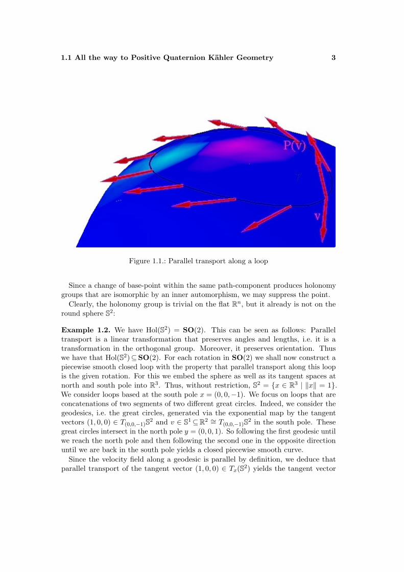
Let us now focus on closed loops based at some x ∈M—cf. figure 1.1. Then paralleltransport is a linear transformation of TxM . We may concatenate two loops γ1, γ2 toγ1 ∗ γ2 as usual. We obtain:
Pγ1∗γ2 = Pγ2 Pγ1
Parallel transport along the “inverse loop” γ−1(t) := γ(1 − t) leads to the inversetransformation:
Pγ−1 = P−1γ
Parallel transport along the constant curve is the identity transformation.
This leads to the following crucial definition:
Definition 1.1. The group
Holx(M, g) = Pγ | γ is a closed loop based at x⊆GL(TxM)
is called the holonomy group of M (at x).
1.1 All the way to Positive Quaternion Kahler Geometry 3
Figure 1.1.: Parallel transport along a loop
Since a change of base-point within the same path-component produces holonomygroups that are isomorphic by an inner automorphism, we may suppress the point.
Clearly, the holonomy group is trivial on the flat Rn, but it already is not on theround sphere S2:
Example 1.2. We have Hol(S2) = SO(2). This can be seen as follows: Paralleltransport is a linear transformation that preserves angles and lengths, i.e. it is atransformation in the orthogonal group. Moreover, it preserves orientation. Thuswe have that Hol(S2)⊆SO(2). For each rotation in SO(2) we shall now construct apiecewise smooth closed loop with the property that parallel transport along this loopis the given rotation. For this we embed the sphere as well as its tangent spaces atnorth and south pole into R3. Thus, without restriction, S2 = x ∈ R3 | ‖x‖ = 1.We consider loops based at the south pole x = (0, 0,−1). We focus on loops that areconcatenations of two segments of two different great circles. Indeed, we consider thegeodesics, i.e. the great circles, generated via the exponential map by the tangentvectors (1, 0, 0) ∈ T(0,0,−1)S2 and v ∈ S1⊆R2 ∼= T(0,0,−1)S2 in the south pole. Thesegreat circles intersect in the north pole y = (0, 0, 1). So following the first geodesic untilwe reach the north pole and then following the second one in the opposite directionuntil we are back in the south pole yields a closed piecewise smooth curve.
Since the velocity field along a geodesic is parallel by definition, we deduce thatparallel transport of the tangent vector (1, 0, 0) ∈ Tx(S2) yields the tangent vector
4 1 Introduction
(−1, 0, 0) in y. (Parallel transport of v along the second geodesic yields −v.) As paralleltransport P preserves angles we see that parallel transport of (−1, 0, 0) ∈ Ty(S2) alongthe inverse second great circle yields the vector P (1, 0, 0) = v2 ∈ S1⊆C ∼= Tx(S2),i.e. the vector in S1 determined by the fact that ^(P (1, 0, 0), (1, 0, 0)) = 2·^(v, (1, 0, 0)).Thus by a suitable choice of v we may realise any given rotation in SO(2).
Recall that a simply-connected Riemannian manifold is irreducible if it does notdecompose as a Cartesian product. It is non-symmetric if it does not admit aninvolutive isometry sp, a geodesic symmetry, for every point p ∈M having this pointas an isolated fixed-point.
We cite the following celebrated theorem due to Berger, 1955—cf. corollary [5].10.92,p. 300:
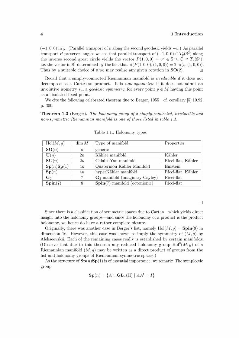
Theorem 1.3 (Berger). The holonomy group of a simply-connected, irreducible andnon-symmetric Riemannian manifold is one of those listed in table 1.1.
Table 1.1.: Holonomy types
Hol(M, g) dimM Type of manifold PropertiesSO(n) n genericU(n) 2n Kahler manifold KahlerSU(n) 2n Calabi–Yau manifold Ricci-flat, KahlerSp(n)Sp(1) 4n Quaternion Kahler Manifold EinsteinSp(n) 4n hyperKahler manifold Ricci-flat, KahlerG2 7 G2 manifold (imaginary Cayley) Ricci-flatSpin(7) 8 Spin(7) manifold (octonionic) Ricci-flat
Since there is a classification of symmetric spaces due to Cartan—which yields directinsight into the holonomy groups—and since the holonomy of a product is the productholonomy, we hence do have a rather complete picture.
Originally, there was another case in Berger’s list, namely Hol(M, g) = Spin(9) indimension 16. However, this case was shown to imply the symmetry of (M, g) byAlekseevskii. Each of the remaining cases really is established by certain manifolds.(Observe that due to this theorem any reduced holonomy group Hol0(M, g) of aRiemannian manifold (M, g) may be written as a direct product of groups from thelist and holonomy groups of Riemannian symmetric spaces.)
As the structure of Sp(n)Sp(1) is of essential importance, we remark: The symplecticgroup
Sp(n) = A⊆GLn(H) | AAt = I

1.1 All the way to Positive Quaternion Kahler Geometry 5
(with quaternionic conjugation defined by (i, j, k) 7→ (−i,−j,−k)) is the quaternionicanalogue of the real respectively complex groups O(n) and U(n). By Sp(n)Sp(1)we denote the group φ(Sp(n)× Sp(1)), where φ : Sp(n)× Sp(1)→ GL2n(C) is therepresentation given by φ((A, h))(x) = Axh−1 with kernel kerφ = 〈−id,−1〉. Thus wehave:
Sp(n)Sp(1) := φ(Sp(n)× Sp(1)) = Sp(n)×Z2 Sp(1) = (Sp(n)× Sp(1))/〈(−id,−1)〉
Definition 1.4. A Quaternion Kahler Manifold is a connected oriented Riemannianmanifold (M4n, g) with holonomy group contained in Sp(n)Sp(1). If n = 1 weadditionally require M to be Einstein and self-dual.
One may use the Levi–Civita connection to define different notions of curvature.Classically, there are three different concepts: sectional curvature, Ricci curvature andscalar curvature, which arise as contractions of the curvature tensor. Indeed, one maydefine the Ricci tensor as the first contraction
Ric(X,Y ) =4n∑i=1
R(Ei, X, Y,Ei)
of the Riemannian curvature tensor
R(X,Y, Z,W ) = g(∇gX∇gY Z −∇
gY∇
gXZ −∇
g[X,Y ]Z,W )
(The vector fields Ei form a local orthonormal basis.) Scalar curvature is the secondcontraction, i.e. the trace
scal(p) =4n∑i=1
Ricp(Ei, Ei)
of the Ricci tensor, where the Ei are orthonormal coordinate vector fields. (By theargument and index p we stress the fact that scalar curvature depends on the pointp ∈ M only.) The sectional curvature along a plane generated by two orthonormalvectors v and w is given by
K(v, w) = R(v, w,w, v)
(This is well-defined, as R(X,Y )Z in a point depends on the values of X, Y , Z in thepoint only.) Ricci-curvature is defined as
ric(v) = Ric(v, v)

6 1 Introduction
Scalar curvature is the weakest notion, sectional curvature the strongest one. A nicedescription of scalar curvature scal(p) is the following one:
Vol(Bε(p))Vol(BEucl
ε (0))= 1− scal(p)
6(n+ 2)ε2 +O(ε4)
That is, scalar curvature measures volume distortion to a certain degree.Quaternion Kahler Manifolds are Einstein (cf. [5].14.39, p. 403), i.e. the Ricci tensor
is a multiple of the metric tensor. Thus we compute
scal(p) =4n∑i=1
Ric(Ei, Ei) = k ·4n∑i=1
gp(Ei, Ei) = 4k · n
and the scalar curvature is constant. This leads to the following crucial definition.
Definition 1.5. A Positive Quaternion Kahler Manifold is a Quaternion KahlerManifold with complete metric and positive scalar curvature.
We present some clarifying facts:
• Just to avoid confusion: A Quaternion Kahler Manifold needs not be Kahlerianin general, since Sp(n)Sp(1) * U(2n). No Positive Quaternion Kahler Manifoldadmits a compatible complex structure (cf. [67].1.3, p. 88).
• The structure group reduces to Sp(n), i.e. M is (locally) hyperKahler if andonly if the scalar curvature vanishes (cf. [5].14.45.a, p. 406 or [67].1.2, p. 87).Little is known in the case of negative scalar curvature.
• A Positive Quaternion Kahler Manifold is necessarily compact and simply-connected (cf. [66], p. 158 and [66].6.6, p. 163).
• A compact orientable (locally) Quaternion Kahler Manifold with positive sec-tional curvature is isometric to the canonical quaternionic projective space(cf. theorem [5].14.43, p. 406).
The only known examples up to now are given by the so-called Wolf spaces , which areall symmetric and which are the only homogeneous examples as a result of Alekseevskiishows (cf. [5].14.56, p. 409). There is an astonishing relation between Wolf spaces andcomplex simple Lie algebras. Indeed, there is a well-understood construction principlewhich involves Lie groups. So there are three infinite series of Wolf spaces and somefurther spaces corresponding to the exceptional Lie algebras (cf. table 1.2). We nowstate the crucial conjecture that motivates the biggest part of our work in this field.
Conjecture 1.6 (LeBrun, Salamon). Every Positive Quaternion Kahler Manifold isa Wolf space.
This conjecture is backed by the following remarkable theorem by Salamon andLeBrun.
1.1 All the way to Positive Quaternion Kahler Geometry 7
Table 1.2.: Wolf spaces
Wolf space M dimM
HPn = Sp(n+ 1)/Sp(n)× Sp(1) 4nGr2(Cn+2) = U(n+ 2)/U(n)×U(2) ordinary type 4nGr4(Rn+4) = SO(n+ 4)/SO(n)× SO(4) 4nG2/SO(4) 8F4/Sp(3)Sp(1) 28E6/SU(6)Sp(1) exceptional type 40E7/Spin(12)Sp(1) 64E8/E7Sp(1) 112
Theorem 1.7 (Finiteness). There are only finitely many Positive Quaternion KahlerManifolds in each dimension.
Proof. See theorem [54].0.1, p. 110, which itself makes use of a classification resultby Wisniewski—see below.
A confirmation of the conjecture (cf. 1.6) has been achieved in dimensions four(Hitchin) and eight (Poon–Salamon, LeBrun–Salamon); if the fourth Betti numberequals one it was shown that in dimensions 12 and 16 the manifold is a quaternionicprojective space—cf. theorem [67].2.1, p. 89.
As we already remarked, it is an astounding fact that the theory of Positive Quater-nion Kahler Manifolds may completely be transcribed to an equivalent theory incomplex geometry. This is done via the twistor space Z of the Positive QuaternionKahler Manifold M . As this connection will be of importance for us, we shall depictsome possible constructions of Z.
Locally the structure bundle with fibre Sp(n)Sp(1) may be lifted to its doublecovering with fibre Sp(n)× Sp(1). The only space that permits such a global lift isthe quaternionic projective space; and, in general, the obstruction to the lifting is aclass in second integral homology generating a Z2-subgroup.
So locally one may use the standard representation of Sp(1) on C2 to associate avector bundle H. In general H does not exist globally but its complex projectivisationZ = PC(H) does. In particular, we obtain the twistor fibration
CP1 → PC(H)→M
An alternative construction of the same manifold Z, which we may also use to shedsome more light on the structure of M , is the following: A hyperKahler manifold maybe defined by three complex structures I, J , K behaving like the unit quaternions i, j,
8 1 Introduction
k, i.e. IJ = −JI = K and I2 = J2 = −id and such that the manifold is Kahlerianwith respect to each of them. On a Quaternion Kahler Manifold M we do not havethese structures globally but only locally. That is, we have a subbundle of the bundleEnd(TM) locally generated by the almost complex structures I, J and K. This canbe seen as follows:
Again locally we lift the Sp(n)Sp(1)-principal bundle to an Sp(n)× Sp(1) bundle.Now we may use the adjoint representation to associate a vector bundle to theprincipal bundle: Indeed, we have the map φ : Sp(1)→ Aut(Sp(1)) given by g 7→ φgwith φg(h) = ghg−1. Since each φg is an automorphism of Sp(1), it induces a mapAdg on the tangent space of the identity element preserving the Lie bracket, i.e. anautomorphism of the Lie algebra sp(1). The map Ad : Sp(1)→ Aut(sp(1)) given byg 7→ Adg is the requested representation.
Note that the center of Sp(1) is ±1. Hence we have φ+1 = φ−1 and ker Ad = ±1.This permits to associate a bundle with respect to the hence well-defined action
(g1, g2) · (p, s) = ((g1, g2) · p,Adg2s)
with p ∈ P , the Sp(n)Sp(1)-principal bundle, s ∈ sp(1) and (g1, g2) ∈ Sp(n)Sp(1).So this globally associates the (three-dimensional) real vector bundle E′, the quotientof P × sp(1) by this action, to the adjoint representation of Sp(1).
Moreover, the Lie algebra of Sp(1) is just
sp(1) = h ∈ H | h+ h = 0.
So sp(1) has the structure of the imaginary quaternions. This means that locally E′
has three sections I, J and K as requested, i.e. three endomorphisms of H with therespective commutating properties. (One may view E′⊆End(TM) as the subbundlegenerated by the three locally defined almost complex structures I, J , K—cf. [5],p. 412.) The twistor space Z of M now is just the unit sphere bundle S(E′) associatedto E′. The twistor fibration is just
S2 → S(E′)→M
(Comparing this bundle to its version above we need to remark that clearly CP1 ∼= S2.)A similar construction leads to a 3-Sasakian manifold S1-fibring over Z (cf. [28]).
As an example one may observe that on HPn we have a global lift of Sp(n)Sp(1)and that the vector bundle associated to Sp(1) is just the tautological bundle. Nowcomplex projectivisation of this bundle yields the complex projective space CP2n+2
and the twistor fibration is just the canonical projection.More generally, on Wolf spaces one obtains the following: The Wolf space may be
written as G/KSp(1) (cf. the table on [5], p. 409) and its corresponding twistor spaceis given as G/KU(1) with the twistor fibration being the canonical projection.
1.1 All the way to Positive Quaternion Kahler Geometry 9
For the construction of the twistor space we used local lifts of Sp(n)Sp(1) toSp(n) × Sp(1). Then there are the standard complex representations of Sp(n) onC2n and of Sp(1) on C2. The bundles associated to these actions will be calledE respectively H. That is, define a right action of Sp(n) on the direct productPSp(n) × C2n of the (local) principal Sp(n)-bundle PSp(n) with C2n by the pointwiseconstruction
(p, v) · g := (p · g, %(g−1)v)
where % is the standard representation of Sp(n). Then form the quotient
E = (PSp(n) × C2n)/Sp(n)
Do the same for
H = (PSp(1) × C2)/Sp(1).
Moreover, we obtain the following formula for the complexified tangent bundle TCMof the Positive Quaternion Kahler Manifold M (cf. [67], p. 93):
TCM = E ⊗H
The bundles E and H arise from self-dual representations and so their odd-degreeChern classes vanish. The Chern classes of E will be denoted by
c2i := c2i(E) ∈ H2i(M)
and
u := −c2(H) ∈ H4(M)
We explicitly draw the reader’s attention to the definition of u as the negative secondChern class of H. We fix this notation once and for all. (By abuse of notation we shallsometimes equally denote a representative of the cohomology class u by u.)
Cohomology will always be taken with rational coefficients unless speci-fied differently.
The quaternionic volume
v = (4u)n ∈ H4n(M4n)
is integral and satisfies 1 ≤ v ≤ 4n—cf. [67], p. 114 and corollary [68].3.5, p. 7.
Let us now state some important facts about twistor spaces.
Theorem 1.8. The twistor space Z of a Positive Quaternion Kahler Manifold is asimply-connected compact Kahler Einstein Fano contact manifold.
10 1 Introduction
Proof. See theorem [54].1.2, p. 113.
The classification of twistor spaces is equivalent to the classification of the manifoldsthemselves. For this recall that two Riemannian manifolds (M1, g1) and (M2, g2) arecalled homothetic if there exists a diffeomorphism φ : M1 →M2 such that the inducedmetric satisfies φ∗g2 = cg1 for some constant c > 0. The map φ then is a homothety.
Theorem 1.9. Two Positive Quaternion Kahler Manifolds are homothetic if and onlyif their twistor spaces are biholomorphic.
Proof. See theorems [54].3.2, p. 119 and [66].4.3, p. 155.
Furthermore, note the following theorem:
Theorem 1.10. If Z is a compact Kahler Einstein manifold with a holomorphiccontact structure, then Z is the twistor space of some Quaternion Kahler Manifold.
Proof. See theorem [67].5.3, p. 102.
Twistor theory has proved to be very fruitful. Apart from the finiteness result(cf. 1.7) above, many properties of Positive Quaternion Kahler Manifolds were gainedvia Fano contact geometry. In the same vein the fact that M is simply-connectedfollows from the result that π1(Z) = 0 via the long exact homotopy sequence: Indeed,the manifold Z has a finite fundamental group—cf. the theorem of Myers, corollary[18].3.2, p. 202—and, as it is Fano, it does not possess finite coverings by the Kodairavanishing theorem—cf. [32], p. 154 and [54], p. 114. Thus we have that π1(Z) = 0.Let us now illustrate the strength of this theory with yet another example.
For Fano manifolds Z there is a contraction theorem which guarantees that there isalways a map of varieties Z → X decreasing the second Betti number by one whilstthe kernel of H2(Z,R)→ H2(X,R) is generated by the class of a rational holomorphiccurve CP1⊆Z. If the second Betti number is one, i.e. b2(Z) = 1, this theorem virtuallydoes not provide any information at all, since X may be taken to be a point. A famoustheorem by Wisniewski now classifies the cases in which b2(Z) > 1 and, surprisingly, itonly yields three possibilities for Z. In the case of contact varieties Z we even obtain
Theorem 1.11. Let Z be a Fano contact manifold satisfying b2(Z) > 1, thenZ = P(T ∗CPn+1).
Proof. See corollary [54].4.2, p. 122.
This is a major tool for the following corollary which, in particular, can be considereda recognition theorem for the complex Grassmannian.
Corollary 1.12 (Strong rigidity). Let (M, g) be a Positive Quaternion Kahler Mani-fold. Then either
π2(M) =
0 iff M ∼= HPn
Z iff M ∼= Gr2(Cn+2)finite with 〈ε〉 ∼= Z2-torsion contained in π2(M) otherwise
1.1 All the way to Positive Quaternion Kahler Geometry 11
Proof. See theorems [54].0.2, p. 110, and [67].5.5, p. 103.
Via the Hurewicz theorem we may identify π2(M) with H2(M,Z). Using universalcoefficients we obtain that H2(M,Z2) is the two-torsion in H2(M,Z), as M is simply-connected. The element ε now corresponds to the obstruction to a global lifting ofSp(n)Sp(1) to Sp(n)× Sp(1) as defined on [66], p. 149. If such a lifting exists, it isshown in theorem [66].6.3, p. 160–162, that the isometry group of the manifold hasto be very large; large enough to identify the manifold as the quaternionic projectivespace.
Let us now collect cohomological properties of Positive Quaternion Kahler ManifoldsM4n. By bi = dimH i(M) we shall denote the Betti numbers of M .
Recall the class u = −c2(H). There is a cohomology class l ∈ H2(Z)—representedby a Kahler form—which generates H∗(Z) as an H∗(M)-module under the restrictionthat l2 = u (cf. [66], p. 148 (and (2.6) on that page), [35], p. 356). This class is givenby l = 1
2c1(L2) for a certain bundle L2 as on [66], p. 148.We shall mainly use the terminology z = l. With respect to this form, the manifold
Z—as it is a Kahler manifold—satisfies the Hard-Lefschetz property: The morphism
Lk : Hn−k(Z,R)→ Hn+k(Z,R) Lk([α]) = [zk ∧ α]
is an isomorphism.
Theorem 1.13 (Cohomological properties). A Positive Quaternion Kahler ManifoldM satisfies:
• Odd-degree Betti numbers vanish, i.e. b2i+1 = 0 for i ≥ 0.
• The identity
n−1∑p=0
(6p(n− 1− p)− (n− 1)(n− 3)
)b2p =
12n(n− 1)b2n
holds and specialises to
2b2 = b6(1.1)−1 + 3b2 + 3b4 − b6 = 2b8(1.2)
−4 + 5b2 + 8b4 + 5b6 − 4b8 = 5b10(1.3)
in dimension 12, 16 and 20 respectively.
12 1 Introduction
• The twistor fibration yields an isomorphism of H∗(M)-modules
H∗(Z) ∼= H∗(M)⊗H∗(S2) ∼= H∗(M)⊕H∗(M)z
• A Positive Quaternion Kahler Manifold M4n 6∼= Gr2(Cn+2) is rationally 3-connected.
• The rational/real cohomology algebra possesses an analogue of the Hard-Lefschetzproperty, i.e. with the four-form u ∈ H4(M) from above the morphism
Lk : Hn−k(M,R)→ Hn+k(M,R) Lk(α) = uk ∧ α
is an isomorphism. In particular, we obtain
bi−4 ≤ bi
for (even) i ≤ 2n. A generator in top cohomology H4n(M) is given by un. Thisdefines a canonical orientation.
Proof. The first point is proven in theorem [66].6.6, p. 163, where it is shown thatthe Hodge decomposition of the twistor space is concentrated in terms Hp,p(Z). Thesecond item is due to [65].5.4, p. 403. The third assertion follows from our remarkbefore stating the theorem. It is actually a consequence of the Hirsch lemma, sincethe spectral sequence of the fibration obviously degenerates at the E2-term (due tovanishing of odd-degree cohomology groups of M).
The manifold M is simply-connected. Due to corollary 1.12 we have that b2 = 0for Mn 6∼= Gr2(Cn+2). By the first point of this theorem we obtain that b3 = 0. SoMn 6∼= Gr2(Cn+2) is rationally 3-connected by the Whitehead theorem.
The Hard-Lefschetz property of M follows from the Hard-Lefschetz property of Z:Indeed, the class z ∈ H2(Z) is a Kahler class and thus M has the Hard-Lefschetzproperty with respect to the class 0 6= u = z2 ∈ H4(M).
So for a Positive Quaternion Kahler Manifold M it is equivalent to demand that Mbe rationally 3-connected—i.e. to have that π1(M)⊗Q = π2(M)⊗Q = π3(M)⊗Q = 0—and to require that M be π2-finite—i.e. to suppose that π2(M) <∞.
The following consequence is as simple as it is astonishing.
Lemma 1.14. Let M be rationally 3-connected of dimension 20 with b4 ≤ 5. Then itholds:
b6 = b10 ∨ (b4, b8) ∈ (1, 1), (2, 3), (3, 5), (4, 7), (5, 9)(1.4)
Proof. By assumption b2 = 0. Equation (1.3) becomes
4(2b4 − b8 − 1) = 5(b10 − b6)
1.1 All the way to Positive Quaternion Kahler Geometry 13
where the right hand side is non-negative due to Hard-Lefschetz (cf. 1.13). Hence theterm 2b4 − b8 − 1 must either be a positive multiple of 5 or zero. Since also b8 ≥ b4,the first case may not occur for b4 ≤ 5. Thus it holds that b6 = b10. The existence ofthe form 0 6= [u] ∈ H4(M) show that b4 ≥ 1.
A recognition theorem which relates cohomology to isometry type is the following:
Theorem 1.15. Let M be a Positive Quaternion Kahler Manifold. If dimM ≤ 16and b4(M) = 1, then M is homothetic to the quaternionic projective space.
Proof. See theorem [67].2.1.ii, p. 89.
We remark that after corollary 1.12—the “strong rigidity” theorem—this is thesecond type of theorem that relates information from algebraic topology to the isometrytype of M . If we wanted to be laconic, we could say that this gives us a feeling ofeven “stronger rigidity”. Section 4.2 of chapter 4 is devoted to this kind of recognitiontheorems. In particular, we shall generalise the theorem in corollary 4.4 respectivelytheorem 4.5 to dimensions 20 and 24 respectively.
Another property of Positive Quaternion Kahler Manifolds related to their coho-mology is the definiteness of the generalised intersection form, which is a symmetricbilinear form. This result was obtained by Fujiki (cf. [27]). He asserted negative orpositive definiteness depending on degrees. Nagano and Takeuchi claim the positivedefiniteness of the intersection form in [61]. So we see that the sign depends on choices.
We shall reprove a precise formulation with our conventions. The theorem will be aconsequence of the Hodge–Riemann bilinear relations on the twistor space Z. Againwe shall use (a representative of) the form u = −c2(H) and the Kahler form l = c1(L).The orientations are naturally given by un on M respectively by l2n+1 on Z.
Theorem 1.16. The generalised intersection form
Q(x, y) = (−1)r/2∫Mx ∧ y ∧ un−r/2
for [x], [y] ∈ Hr(M4n,R) with even r ≥ 0 is positive definite. In particular, thesignature of the manifold satisfies
sign(M) = (−1)nb2n(M)
Proof. Recall that the Hodge decomposition of the twistor space Z of real dimension4n+ 2 is given by
Hr(Z,C) = Hr/2,r/2(Z),
14 1 Introduction
for all r ≥ 0; i.e. all the groups Hp,q(Z) with p 6= q vanish—cf. the proof of theorem[66].6.6, p. 163, respectively formula (6.4) on that page. We consider the Lefschetzdecomposition (cf. [32], p. 122) on the complex cohomology of Z:
Hr(Z,C) = Hr/2,r/2(Z) =∑
s≥maxr−(2n+1),0
LsHr/2−s,r/2−s0 (Z)
where H∗0 (·) denotes primitive cohomology (cf. [32], p. 122) and Ls(x) = ls ∧ x.Recall the twistor fibration CP1 → Z
π−→M with the Leray-Serre spectral sequencedegenerating at the E2-term. Thus for r ∈ Z we obtain that
Hr(Z,R) = π∗Hr(M,R)⊕ π∗Hr−2(M,R) · l
This formula holds with real coefficients. Tensoring with C makes it valid withcomplex coefficients. More precisely, we obtain the subalgebra (π∗Hr(M,R))⊗ C of(complexified) real forms. That is, an element in (π∗Hr(M,R)) ⊗ C is of the formη + η for η ∈ Hr(Z,R).
We combine this with the Lefschetz decomposition of Z and compute
Hr(Z,C) =
∑s≥maxr−(2n+1),0
s even
LsHr/2−s,r/2−s0 (Z)
+
∑s≥maxr−(2n+1),0
s even
LsHr/2−s,r/2−s0 (Z)
· lSince l2 = u this grading actually enforces
π∗Hr(M,C) =∑
s≥maxr−(2n+1),0s even
LsHr/2−s,r/2−s0 (Z)(1.5)
From theorem [75].V.6.1, p. 203, we cite that—on a compact Kahler manifold X (ofreal dimension 2k)—the form
Q(η, µ) =∑
maxs≥(r−k),0
(−1)[r(r+1)/2]+s
∫XLk−r+2s(ηs ∧ µs)
with Lefschetz decompositions η =∑Lsηs ∈ Hr(X,C) and µ =
∑Lsµs ∈ Hr(X,C),
i.e. with primitive ηs, µs, satisfies
Q(η, Jη) > 0
1.1 All the way to Positive Quaternion Kahler Geometry 15
for η 6= 0 and J =∑
p,q ip−qΠp,q with canonical projections
Πp,q : Hp+q(X,C)→ Hp,q(X).
So in the case of the twistor space X = Z we have J = id, since Hp,p(Z) =H2p(Z,C). Let 0 6= η = Lsη′ be a real form in H2p(Z,C), i.e. η = η′ + η′ as aboveand η = η, with primitive η′. Then we have that η ∈ Hp,p(Z), which is equivalent toη′ ∈ Hp−s,p−s
0 (Z) = H2(p−s)0 (Z,C). Hence it holds that
Q(η, η) = Q(η, Jη) > 0
So we obtain (with r = 2p):
0 < Q(η, η)
= (−1)[2p(2p+1)/2]+s
∫ZL2n+1−2p+2s(η′ ∧ η′)
= (−1)s+p∫Zl2(n−p+s)+1 ∧ η′ ∧ η′
= (−1)s+p∫Zl2(n−p)+1 ∧ η ∧ η
(1.6)
Now let η be an arbitrary element in π∗Hr(M,R)⊗C. Then η is real and accordingto (1.5) we have
η =∑s even
ls ∧ ηs
with primitive ηs.Hence by (1.6) we derive that
0 <∑s even
(−1)s+p∫Zl2(n−p+s)+1 ∧ ηs ∧ ηs
=∑s even
(−1)p∫Zl2(n−p+s)+1 ∧ ηs ∧ ηs
= (−1)r/2∫Zl2n−r+1 ∧ η ∧ η
for 0 6= η ∈ π∗Hr(M,C). The twistor transform finally yields the assertion as we have:
(−1)r/2∫Mun−r/2 ∧ η ∧ η = (−1)r/2
∫Zl2n−r+1 ∧ η ∧ η > 0
16 1 Introduction
We remark that in low dimensions (dimM ≤ 20) this result fits to the computationof the signature of the Positive Quaternion Kahler Manifold M via the L-genus(combined with further equations obtained by Index Theory)—cf. chapter 4.
An oriented compact manifold M4n is called spin if its SO(4n)-structure bundlelifts to a Spin(4n)-bundle, or equivalently, its second Stiefel-Whitney class w2(M) = 0vanishes. A vector bundle E → M is called spin if w1(E) = w2(E) = 0. (Thus amanifold is spin iff its tangent bundle is spin.)
Positive Quaternion Kahler Manifolds M4n 6= HPn are spin if and only if n is even.Indeed, the second Stiefel-Whitney class w2(M) satisfies
w2(M) =
ε for odd n
0 for even n
where ε is the obstruction class to a global lifting of Sp(n)Sp(1)—cf. proposition[66].2.3, p. 148.
Now Index Theory enters the stage. This approach led to some striking results andis likely to be fruitful in the future, too: Via Index Theory an alternative proof of theclassification in dimension 8 was obtained (cf. theorem [54].5.4, p. 129), theorem 1.15was established and the relations on Betti numbers in theorem 1.13 were found. Theresults on the isometry groups in dimensions 12 and 16 in theorem 1.18 below are alsoa consequence of Index Theory.
Let us briefly mention some basic notions from Index Theory. For general referencewe recommend the textbooks [40] and [52].
A genus φ is a ring homomorphism φ : Ω⊗Q→ R from the rationalised orientedcobordism ring Ω⊗Q into an integral domain R over Q.
Let Q(x) = 1 + a2x2 + a4x
4 + . . . be an even power series with coefficients in R.Assume the xi to have degree 2. The product Q(x1) · · · · ·Q(xn) is symmetric in the x2
i .Therefore it may be expressed as a series in the elementary symmetric polynomials piof the x2
i . The term of degree 4r is given by Kr(p1, . . . , pr), i.e.
Q(x1) · · · · ·Q(xn) =1 +K1(p1) +K2(p1, p2) + . . .
+Kn(p1, . . . , pn) +Kn+1(p1, . . . , pn, 0) + . . .
On a compact oriented differentiable manifold M4n the genus φQ : Ω ⊗ Q → Rasociated to the power series Q is defined by
φQ(M) = Kn(p1, . . . , pn)[M ]
where pi = pi(M) ∈ H4i(M,Z) are the Pontryagin classes of M . (On such manifoldswith dimension not divisible by four the genus is set to zero.)
1.1 All the way to Positive Quaternion Kahler Geometry 17
Prescribing the values of a genus on the complex projective spaces leads to a powerseries Q as above. As a consequence we see that there is a one-to-one correspondencebetween such power series and genera.
The genus φQ corresponding to the power series Q(x) = x/2sinh(x/2) is called the
A-genus; the genus φQ corresponding to Q(x) = xtanhx is the L-genus.
On a 4n-dimensional spin manifold M one may define an elliptic differential operator
D/ : Γ(S+)→ Γ(S−)
called the Dirac operator . (The spinor bundle S of TM splits into the eigenbundlesS+ and S− of a certain involution in the Clifford bundle Cl(M) of the tangent bundleTM .) The index of D/ is given by
ind(D/) = kerD/− cokerD/
In the same way one may construct twisted Dirac operators: In order to obtain atwisted Dirac operator locally defined by
D/(E) : Γ(S+ ⊗ E)→ Γ(S− ⊗ E)
we may use a similar definition for certain vector bundles E.As a consequence of the famous Atiyah–Singer Index Theorem we obtain
ind(D/(E)) = 〈A(M) · ch(E), [M ]〉
Thus we see that the Index Theorem interlinks the concept of indices of differentialoperators with the notion of genera.
On a Positive Quaternion Kahler Manifold M4n we have the locally associatedbundles E and H from above. Now form the (virtual) bundles∧k
0E :=
∧k E −
∧k−2E
of exterior powers and the bundles
SlH := SymlH
of symmetric powers. Set
ik,l := indD/(∧k
0E ⊗ SlH
)The bundles S± ⊗
∧k
0E ⊗ SlH exist globally if and only if n+ k + l is even. In this
case, using the index theorem one obtains the following relations (cf. [67], p. 117):
18 1 Introduction
Theorem 1.17. It holds:
ik,l =
0 if k + l < n
(−1)k(b2p(M) + b2p−2(M)) if k + l = n
d if k = 0, l = n+ 2
where d = dim Isom(M) is the dimension of the isometry group of M and the bi(M)are the Betti numbers of M as usual.
There is the following information on isometry groups:
Theorem 1.18. Let M4n be a Positive Quaternion Kahler Manifold with isometrygroup Isom(M). We obtain:
• The rank rk Isom(M) may not exceed n + 1. If rk Isom(M) = n + 1, thenM ∈ HPn,Gr2(Cn+2).
• If rk Isom(M) ≥ n2 + 3, then M is isometric to HPn or to Gr2(Cn+2).
• It holds that dim Isom(M4n) ≤ dim Sp(n+ 1) = (n+ 1)(2n+ 3). Equality holdsif and only if M ∼= HPn.
• If n = 3, then dim Isom(M) ≥ 5; if n = 4, then dim Isom(M) ≥ 8.
Proof. The first assertion is due to theorem [67].2.1, p. 89. The second item istheorem [20].1.1, p. 642. The inequality in the third assertion follows from corollary[68].3.3, p. 6. In case dim Isom(M) = (n+ 1)(2n+ 3) it was already observed on [66],p. 161 that M is homothetic to the quaternionic projective space. The fourth point isdue to theorem [66].7.5, p. 169.
The isometry group Isom(M) of M is a compact Lie group. The subsequent lemmapermits a better understanding of Isom(M).
Lemma 1.19. Let G be a compact connected Lie group. Then we obtain:
• The group G possesses a finite covering which is isomorphic to the direct productof a simply-connected Lie group G and a torus T . In particular, G is alsocompact.
• The group G is semi-simple if and only if its fundamental group π1(G) is finite.
Proof. See theorems [11].V.8.1, p. 233, and [11].V.7.13, p. 229.
1.1 All the way to Positive Quaternion Kahler Geometry 19
Table 1.3.: Classification of simple Lie groups up to coveringstype corresponding Lie group dimension
(not necessarily simply-connected)An, n = 1, 2, . . . SU(n+ 1) n(n+ 2)Bn, n = 1, 2, . . . SO(2n+ 1) n(2n+ 1)Cn, n = 1, 2, . . . Sp(n) n(2n+ 1)Dn, n = 3, 4, . . . SO(2n) n(2n− 1)G2 Aut(O) 14F4 Isom(OP2) 52E6 Isom((C⊗O)P2) 78E7 Isom((H⊗O)P2) 133E8 Isom((O⊗O)P2) 248the index n denotes the rank
Consequently, up to finite coverings we may assume that Isom0(M) is the productof a simply-connected semi-simple Lie group—i.e. the product of simply-connectedsimple Lie groups—and a torus.
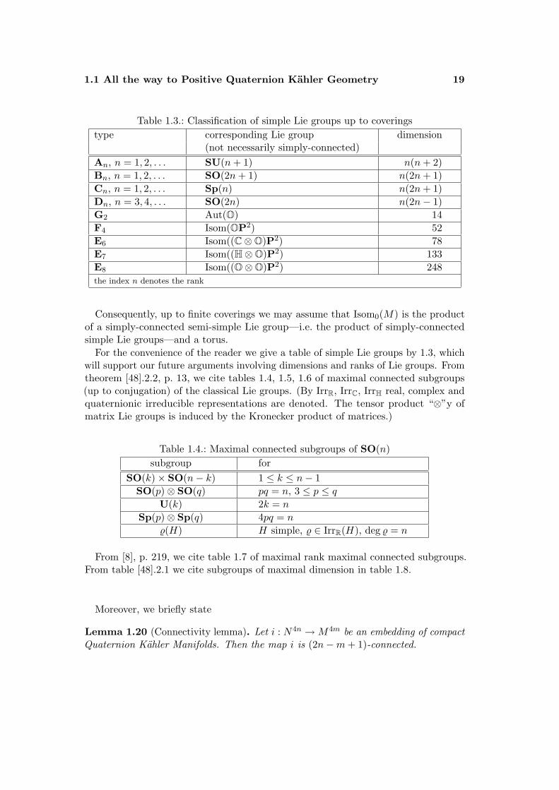
For the convenience of the reader we give a table of simple Lie groups by 1.3, whichwill support our future arguments involving dimensions and ranks of Lie groups. Fromtheorem [48].2.2, p. 13, we cite tables 1.4, 1.5, 1.6 of maximal connected subgroups(up to conjugation) of the classical Lie groups. (By IrrR, IrrC, IrrH real, complex andquaternionic irreducible representations are denoted. The tensor product “⊗”y ofmatrix Lie groups is induced by the Kronecker product of matrices.)
Table 1.4.: Maximal connected subgroups of SO(n)subgroup for
SO(k)× SO(n− k) 1 ≤ k ≤ n− 1SO(p)⊗ SO(q) pq = n, 3 ≤ p ≤ q
U(k) 2k = n
Sp(p)⊗ Sp(q) 4pq = n
%(H) H simple, % ∈ IrrR(H), deg % = n
From [8], p. 219, we cite table 1.7 of maximal rank maximal connected subgroups.From table [48].2.1 we cite subgroups of maximal dimension in table 1.8.
Moreover, we briefly state
Lemma 1.20 (Connectivity lemma). Let i : N4n →M4m be an embedding of compactQuaternion Kahler Manifolds. Then the map i is (2n−m+ 1)-connected.
20 1 Introduction
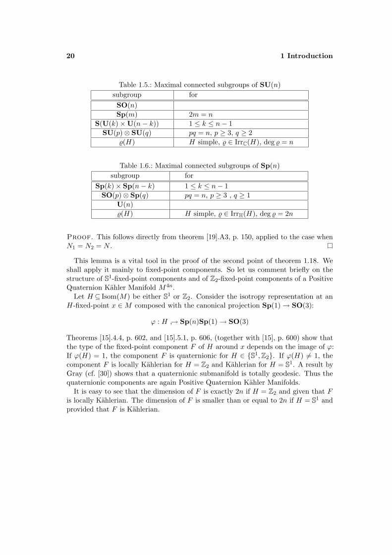
Table 1.5.: Maximal connected subgroups of SU(n)subgroup forSO(n)Sp(m) 2m = n
S(U(k)×U(n− k)) 1 ≤ k ≤ n− 1SU(p)⊗ SU(q) pq = n, p ≥ 3, q ≥ 2
%(H) H simple, % ∈ IrrC(H), deg % = n
Table 1.6.: Maximal connected subgroups of Sp(n)subgroup for
Sp(k)× Sp(n− k) 1 ≤ k ≤ n− 1SO(p)⊗ Sp(q) pq = n, p ≥ 3 , q ≥ 1
U(n)%(H) H simple, % ∈ IrrH(H), deg % = 2n
Proof. This follows directly from theorem [19].A3, p. 150, applied to the case whenN1 = N2 = N .
This lemma is a vital tool in the proof of the second point of theorem 1.18. Weshall apply it mainly to fixed-point components. So let us comment briefly on thestructure of S1-fixed-point components and of Z2-fixed-point components of a PositiveQuaternion Kahler Manifold M4n.
Let H ⊆ Isom(M) be either S1 or Z2. Consider the isotropy representation at anH-fixed-point x ∈M composed with the canonical projection Sp(1)→ SO(3):
ϕ : H → Sp(n)Sp(1)→ SO(3)
Theorems [15].4.4, p. 602, and [15].5.1, p. 606, (together with [15], p. 600) show thatthe type of the fixed-point component F of H around x depends on the image of ϕ:If ϕ(H) = 1, the component F is quaternionic for H ∈ S1,Z2. If ϕ(H) 6= 1, thecomponent F is locally Kahlerian for H = Z2 and Kahlerian for H = S1. A result byGray (cf. [30]) shows that a quaternionic submanifold is totally geodesic. Thus thequaternionic components are again Positive Quaternion Kahler Manifolds.
It is easy to see that the dimension of F is exactly 2n if H = Z2 and given that Fis locally Kahlerian. The dimension of F is smaller than or equal to 2n if H = S1 andprovided that F is Kahlerian.
1.1 All the way to Positive Quaternion Kahler Geometry 21
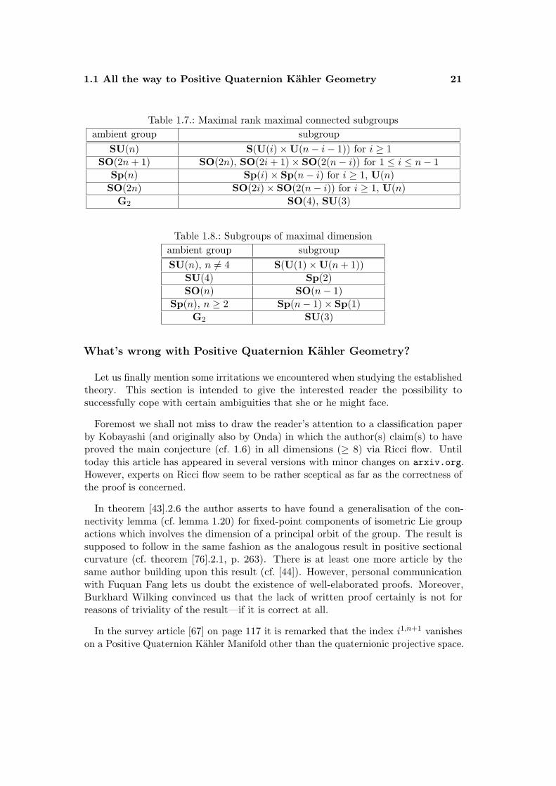
Table 1.7.: Maximal rank maximal connected subgroupsambient group subgroup
SU(n) S(U(i)×U(n− i− 1)) for i ≥ 1SO(2n+ 1) SO(2n), SO(2i+ 1)× SO(2(n− i)) for 1 ≤ i ≤ n− 1
Sp(n) Sp(i)× Sp(n− i) for i ≥ 1, U(n)SO(2n) SO(2i)× SO(2(n− i)) for i ≥ 1, U(n)
G2 SO(4), SU(3)
Table 1.8.: Subgroups of maximal dimensionambient group subgroupSU(n), n 6= 4 S(U(1)×U(n+ 1))
SU(4) Sp(2)SO(n) SO(n− 1)
Sp(n), n ≥ 2 Sp(n− 1)× Sp(1)G2 SU(3)
What’s wrong with Positive Quaternion Kahler Geometry?
Let us finally mention some irritations we encountered when studying the establishedtheory. This section is intended to give the interested reader the possibility tosuccessfully cope with certain ambiguities that she or he might face.
Foremost we shall not miss to draw the reader’s attention to a classification paperby Kobayashi (and originally also by Onda) in which the author(s) claim(s) to haveproved the main conjecture (cf. 1.6) in all dimensions (≥ 8) via Ricci flow. Untiltoday this article has appeared in several versions with minor changes on arxiv.org.However, experts on Ricci flow seem to be rather sceptical as far as the correctness ofthe proof is concerned.
In theorem [43].2.6 the author asserts to have found a generalisation of the con-nectivity lemma (cf. lemma 1.20) for fixed-point components of isometric Lie groupactions which involves the dimension of a principal orbit of the group. The result issupposed to follow in the same fashion as the analogous result in positive sectionalcurvature (cf. theorem [76].2.1, p. 263). There is at least one more article by thesame author building upon this result (cf. [44]). However, personal communicationwith Fuquan Fang lets us doubt the existence of well-elaborated proofs. Moreover,Burkhard Wilking convinced us that the lack of written proof certainly is not forreasons of triviality of the result—if it is correct at all.
In the survey article [67] on page 117 it is remarked that the index i1,n+1 vanisheson a Positive Quaternion Kahler Manifold other than the quaternionic projective space.
22 1 Introduction
The given reference (cf. [53]), however, only seems to prove i1,n+1 ≤ 0. Unfortunately,also the powerful methods developed by Uwe Semmelmann and Gregort Weingartdid not result in a confirmation of the assertion. As Uwe Semmelmann found out,originally also Simon Salamon considered the statement to be rather of conjecturalnature. We want to encourage the reader to prove the result himself, as it has immenseconsequences at least in low dimensions—see for example theorem 4.11.
Note that theorem [35].1.1, p. 2, asserts that a 16-dimensional Positive QuaternionKahler Manifold has fourth Betti number b4 6= 2. In the proof of the theorem b4 = 2is led to a contradiction. In claim 1 on page 4 it is asserted that c2 is not proportionalto u as this would lead to M ∼= HP4. This is supposed to follow directly from a resultin [28]. Indeed, theorem [28].5.1, p. 62, states that if b4 = 1, which implies that c2
necessarily is a multiple of u in particular, then M ∼= HP4. However, the computationsin this proof make use of b4 = 1 and one has to do separate computations for the caseb4 = 2 to confirm the result.
Finally, we point to chapter 2, where we explain why the classification of 12-dimensional Positive Quaternion Kahler Manifolds established in [35] is erroneous anddoes no longer persist.
1.2. A brief history of Rational Homotopy Theory
Homotopy groups are an intriguing field of study: They may be defined in a verybasic way. Yet, their computation turns out to be extremely difficult. So till todaythere is not even a complete picture of the homotopy groups of spheres. It was astriking observation by Quillen and Sullivan that “rationalising the groups” made thesituation much simpler. This can be observed on spheres already as for example
π2n(S2n)⊗Q = π4n−1(S2n)⊗Q = Q
and all the other groups vanish rationally. Moreover, Quillen and Sullivan manageda translation into algebra. This gave birth to Rational Homotopy Theory . Over theyears this theory has been well-elaborated and it has become a powerful and highlyelegant tool.
As a main reference we want to recommend the book [22]. Throughout the dis-sertation we shall follow its conceptual approach and its notation unless indicateddifferently. Let us now review some basic notions we shall need in the main part of thethesis. We do not even attempt to provide a “complete”—of any kind—introductionto the topic. Likewise, we shall not cite lengthy but standard definitions, which allcan be found in the literature, for the general theory. Our goal is to motivate and toguide through the well-established notions and to be more precise when concepts are
1.2 A brief history of Rational Homotopy Theory 23
of greater importance for our present work or if they are more particular in nature.We shall give references whenever parts of the theory are not covered by [22].
Although the theory may be presented in larger generality (e.g. for nilpotent spaces),we make the following general assumption:
Throughout this chapter the spaces in consideration are assumed to besimply-connected (which comprises being path-connected). So are thecommutative differential graded algebras A, i.e. A0 is one-dimensional andA1 = 0. Cohomology will always be taken with rational coefficients when-ever coefficients are suppressed.
Part 1.. . . wherein we shall describe some basic concepts of Rational Ho-motopy Theory.
The rational homotopy type of a simply-connected topological space X is thehomotopy type of a rationalisation XQ of X. By the definition of rationalisationthere is a rational homotopy equivalence φ : X '−→ XQ, i.e. a morphism inducingisomorphisms
π∗(X)⊗Q∼=−→ π∗(XQ)
on homotopy groups. The rationalisation XQ can always be constructed, it can begiven the structure of a CW -complex and it is unique up to homotopy (cf. [22].9.7).By the Whitehead-Theorem π∗(φ) being an isomorphism is equivalent to H∗(φ) beingan isomorphism. Spaces X and Y have the same rational homotopy type, i.e. X 'Q Y ,iff there is a finite chain of rational homotopy equivalences (cf. [22].9.8)
X'−→ . . .
'←− . . . '−→ . . .'←− Y
The transition into algebra is mainly given by the functor APL which replaces thespace X by the commutative differential graded algebra APL(X) (cf. [22].3, [22].10).This functor is a local system APL(·) on the simplicial set of singular simplices ofX. On a smooth manifold M it is sufficient to consider the commuative differentialgraded algebra—over the reals(!)—ADR(M) of ordinary differential forms instead of thepolynomial differential forms APL(M). Yet observe that the ordinary cochain algebraof singular simplices is not commutative so that this new concept really is necessary. Avery brief description of APL could be that to first construct the algebra of polynomialdifferential forms APLn on an ordinary affine n-simplex by simply restricting ordinarydifferential forms (with Q-coefficients). Then the polynomial p-forms of X are thesimplicial set morphisms assigning to a singular n-simplex in X a polynomial p-formin APLn.
24 1 Introduction
A morphism φ of commutative differential graded algebras (A,d) and (B, d) is calleda quasi-isomorphism if H∗(φ) : H(A)→ H(B) is an isomorphism. A weak equivalencebetween A and B, i.e. A ' B, is a finite chain of quasi-isomorphisms:
A'−→ . . .
'←− . . . '−→ . . .'←− B
This may be regarded as an algebraic analogue of a rational homotopy equivalence.Indeed, the functor APL now connects the topological world to the algebraic one
in a very beautiful way: Focussing on simply-connected spaces and algebras bothhaving additionally rational cohomology of finite type, there is a 1-1-correspondence(cf. [22].10):
rational homotopytypes
APL−−→
weak equivalence classes of
commutative cochain algebras
Recall that a graded vector space V =
⊕i V
i is called of finite type if each V i isfinite-dimensional. A cochain algebra is a differential graded algebra concentrated innon-negative degrees. There is a procedure of spatial realisation (cf. [22].17) whichreverses APL to a certain degree by constructing a CW -complex from a commutativecochain algebra.
By this bijection we need no longer differentiate between (weak equivalence classesof) commutative cochain algebras and (homotopy types of) topological spaces.
As a preliminary conclusion we observe that the rational homotopy type of a spaceX is encoded in APL(X) up to weak equivalence and so is the real homotopy type ofa smooth manifold M with respect to ADR(M).
In order to be able to do effective computations one may find some sort of “stan-dard form” within the weak equivalence class, a so-called minimal Sullivan algebra—cf. [22].12. This commutative differential graded algebra is built upon the tensorproduct
∧V = Sym(V even) ⊗
∧(V odd) of the polynomial algebra in even degrees
with the exterior algebra in odd degrees of the graded vector space V . Minimalityis established by requiring that the differential may not hit an element that is notdecomposable. An element in
∧V is called decomposable if it is a linear combination
of non-trivial products of elements of lower degree. More precisely, minimality is givenby
im d⊆∧>0
V ·∧>0
V
A (minimal) Sullivan model for a commutative cochain algebra (A,d) respectively atopological space X is a quasi-isomorphism
m :(∧
V,d) '−→ (A, d)
1.2 A brief history of Rational Homotopy Theory 25
respectively
m :(∧
V,d) '−→ (APL(X), d)
with a (minimal) Sullivan algebra(∧
V,d).
Before we shall continue to describe the theory we shall comment briefly on notation.Otherwise, there might be room for equivocation. Although the following does notdiffer from the standard notation in [22], it might be adequate to state it at this initialpoint of the introduction in a condensed form.
Let V =⊕
i Vi be a graded vector space. By V k we denote its k-th degree subspace
and we shall use the terminology V ≤k =⊕
i≤k Vi, V >0 =
⊕i>0 V
i, . . . . By∧V we
denote, as described, the free commutative graded algebra (cf. example [22].3.6, p. 45)over V . We shall use the term
∧k V to denote all the elements of∧V that have
word-length k in V . So, for example,∧>0 V refers to all the elements that can be
written as sums of real products of elements in V . Finally, it is not surprising that thegrading
(∧V)k = x ∈
∧V | deg x = k again refers to degree.
Let us give two examples of constructions of Sullivan models in special situations.We stress that the models will not be minimal in general.
First, we shall deal with fibrations. Here a Sullivan model for the total space isconstructed out of the Sullivan models of fibre and base space. Let
F → E → B
be a fibration of path-connected spaces. Suppose that B is simply-connected and thatone of H∗(F ), H∗(B) has finite type. Suppose that
(∧VB,d
)→ (APL(B),d) is a
Sullivan model and that(∧
VF , d)→ (APL(F ), d) is a minimal Sullivan model. We
then have
Theorem 1.21. There is a Sullivan model(∧
VB ⊗∧VF , d
)→ (APL(E),d) such
that(∧
VB,d)
is a subcochain algebra of(∧
VB ⊗∧VF , d
). Moreover, it holds for
v ∈ VB that dv − dv ∈∧>0 VB ⊗
∧VF .
Proof. See the corollary on [22], p. 199.
Even if we choose minimal Sullivan models for base and fibre the model of the totalspace needs not be minimal. We shall refer to this model as the model of the fibration.
An application of this model to homogeneous spaces provides a model for G/Hbased upon models for the groups G and H—the second example we shall display.
Let H be a closed connected subgroup of a connected Lie group G. Denote byj : H → G the inclusion and by BH and BG the corresponding classifying spaces of
26 1 Introduction
H and G. It is known (cf. [22], example 12.3, p. 143) that H-spaces—and Lie groupsin particular—admit minimal models of the form(∧
VG, 0)→ (APL(G), d) and
(∧VH , 0
)→ (APL(H),d)
A direct consequence are the minimal models(∧V +1G , 0
)→ (APL(BG), d) and
(∧V +1H , 0
)→ (APL(BH), d)
which arise from a degree-shift of +1 applied to the graded vector spaces VG and VHlying at the basis of the minimal models of G and H (cf. [22].15.15, p. 217). That is,VBG := V +1
G and VBH := V +1H . Let x1, . . . , xr be a homogeneous basis of VG. Thus we
have a corresponding basis x1, . . . , xr of VBG by degree-shift.
Theorem 1.22. The Sullivan algebra(∧
VBG ⊗∧VG, d
)defined by d|VBH
= 0 andby dxi = H∗(B(j))xi for 1 ≤ i ≤ r is a Sullivan model for G/H.
Proof. See proposition [22].15.16, p. 219.
Again, this model by no reasons has to be minimal. This approach can be generalisedto the case of biquotients:
Let G be a compact connected Lie group and let H ⊆G×G be a closed Lie subgroup.Then H acts on G on the left by (h1, h2) · g = h1gh
−12 . The orbit space of this action
is called the biquotient GH of G by H. If H is of the form H = H1 × H2 withinclusions given by H1⊆G× 1⊆G×G and H2⊆1 ×G⊆G×G, we shall alsouse the notation H1\G/H2 instead of GH. If the action of H on G is free, then GHpossesses a manifold structure. This is the only case we shall consider. Clearly, thecategory of biquotients contains the one of homogeneous spaces.
In the notation from above we see that a minimal model for G × G is given by(∧VG×G, 0
)defined by
VG×G = 〈x1, . . . , xr, y1, . . . yr〉
where the yi satisfy deg xi = deg yi. Thus we obtain VBG×BG = 〈x1, . . . , xr, y1, . . . yr〉.Denote by j the inclusion H → G×G. Then we obtain
Theorem 1.23. The Sullivan algebra(∧VBH ⊗
∧〈q1, . . . , qr〉,d
)with d|∧VBH
= 0 and defined by d(qi) = H∗(Bj)(xi − yi) for 1 ≤ i ≤ r is a Sullivanmodel for GH.
Proof. See proposition [42].1, p. 2.
1.2 A brief history of Rational Homotopy Theory 27
Now we present an algorithm that iteratively constructs a minimal model in thecase of a trivial differential. This algorithm is adapted from [22], p. 144–145 from thegeneral case to the case d = 0 that will be of interest for us.
Algorithm 1.24. Let (A, 0) be a commutative differential graded algebra with A0 = Qand A1 = 0. Then the following procedure produces a minimal Sullivan model for (A, 0).
Choose m2 : (∧V 2, 0) → (A, 0) such that H2(m2) : V 2
∼=−→ A2 is anisomorphism.Suppose now mk : (
∧V ≤k, d)→ (A, 0) has been constructed for some k ≥ 2.
Then we may extend this morphism to mk+1 : (∧V ≤k+1, d) → (A, 0) by
the following procedure:Choose elements ai ∈ Ak+1 such that
Ak+1 = imHk+1(mk)⊕⊕i
Q · [ai]
and choose cocyles zj ∈ (∧V ≤k)k+2 such that
kerHk+2(mk) =⊕j
Q · [zj ]
Let V k+1 be a vector space (in degree k + 1) with basis vi, . . . , wj , . . . inone-to-one correspondence with the elements ai respectively zj. Write∧V ≤k+1 =
∧V ≤k⊗
∧V k+1. Extend d to a derivation in
∧V ≤k+1 and mk
to a morphism mk+1 :∧V ≤k+1 → A of graded algebras by setting
dvi = 0, dwj = zj and mk+1vi = ai, mk+1wj = 0.
Observe that the ai and zj can be interpreted in the following way: One may regardimHk+1(mk) as the “surviving products” of lower degrees and thus the ai represent“new” generators, i.e. generators of Ak+1 that are not a linear combination of productsof lower degree. Conversely, the zj are placed—so to say—one for each vanishing linearcombination; i.e. if a linear combination of products in degree k + 2 vanishes (in A),one sets a generator in degree k+ 1 (in V ), which corrects this deviation from freenessby means of d.
Finally note the following simple property.
Proposition 1.25. Let a cochain algebra(∧
V,d)
satisfy the properties
V = V ≥2 and im d⊆∧>0
V ·∧>0
V
Then this algebra is necessarily a minimal Sullivan algebra.
28 1 Introduction
Proof. We elaborate the arguments in [22], example 12.5, p. 144: As a filtration onV we use the filtration on degrees: V (k) :=
⊕ki=1 V
k. Then trivially V =⋃∞k=0 V (k),
V (0)⊆V (1)⊆V (2)⊆ . . . and d = 0 in V (0) = V 0 = Q. We have d : V k →∧k+1 V
by definition and thus d : V k →(∧>0 V ·
∧>0 V)k+1 by assumption. Moreover,
(∧>0V ·
∧>0V)k+1⊆
∧V ≤k−1
since V 1 = 0. Hence
d : V (k) =k⊕i=0
V i →k+1⊕i=0
(∧>0V ·
∧>0V)i⊆∧( k−1⊕
i=0
V i
)=∧V (k − 1)
for k ≥ 1. This reveals(∧
V,d)
as a Sullivan algebra. Minimality is clear byassumption.
The most prominent theorem of Rational Homotopy Theory now connects thegraded vector space V upon which the minimal model
(∧V,d
)of a topological space
X is based with the rational homotopy groups of X. Let K be a field of characteristiczero.
Theorem 1.26. Suppose that X is simply-connected and H∗(X,K) has finite type.Then there is an isomorphism of graded vector spaces
νX : V∼=−→ HomZ(π∗(X),K)
Proof. See theorem [22].15.11, p. 208.
In particular, up to duality, the rational vector space πi(X) ⊗ Q in degree i ≥ 2corresponds exactly to V i. This provides a tremendously effective way of computingrational homotopy!
A topological space X is called n-connected if for 0 ≤ i ≤ n it holds πi(X) = 0. Inthis vein we shall call X rationally n-connected if for 0 ≤ i ≤ n it holds πi(X)⊗Q = 0.Thus for the minimal model of a simply-connected space X with homology of finitetype this is equivalent to V i = 0 for 0 ≤ i ≤ n.
Remark 1.27. Recall the Hurewicz homomorphism hur : π∗(X)→ H∗(X,Z) (cf. [22],p. 58). We have H>0
(∧V,d
)= ker d/im d, where im d⊆
∧≥2 V by minimality. Letζ : H>0
(∧V,d
)→ V be the linear map defined by forming the quotient with
∧≥2 V ,i.e. the natural projection
ζ : ker d/im d→ ker d/((∧≥2
V
)∩ ker d
)⊆V
1.2 A brief history of Rational Homotopy Theory 29
There is a commutative square (cf. [22], p. 173 and the corollary on [22], p. 210)
H>0(∧
V,d) ∼= //
ζ
H>0(X)
hur∗
V νX
∼= // Hom(π>0(X),Q)
where hur∗ is the dual of the rationalised Hurewicz homomorphism. Thus by thissquare ζ and hur∗ are identified.
In particular, we see that if hur⊗Q is injective, then hur∗ is surjective and so is ζ.In such a case every element x ∈ V is closed and defines a homology class.
Part 2.. . . wherein we shall outline the notion of formality.As we have seen, the rational (respectively real) homotopy type of a space X
(respectively a smooth manifold M) is given by APL(X) (respectively ADR(M)). Aprominent question in Rational Homotopy Theory is the following: When can wereplace APL(X) by the cohomology algebra H∗(X) without losing information? Whenis the rational homotopy type of X encoded in its rational cohomology algebra?
Let K be a field of characteristic zero and (A,d) a connected commutative cochainalgebra over K.
Definition 1.28. The commutative differential graded algebra (A,d) is called formal ifit is weakly equivalent to the cohomology algebra (H(A,K), 0) (with trivial differential).
We call a path-connected topological space formal if its rational homotopy type is aformal consequence of its rational cohomology algebra, i.e. if (APL(X), d) is formal. Indetail, the space X is formal if there is a weak equivalence (APL(X),d) ' (H∗(X), 0),i.e. a chain of quasi-isomorphisms
(APL(X), d) '←− . . . '−→ . . .'←− . . . '−→ (H∗(X), 0)
Theorem 1.29. Let X have rational homology of finite type. The algebra(APL(X,K),d) is formal for any field extension K⊇Q if and only if X is a formalspace.
Proof. See [22], p. 156 and theorem 12.1, p. 316.
Corollary 1.30. A compact connected smooth manifold is formal iff there is a weakequivalence (ADR(M),d) ' (H∗(M,R), 0).
Example 1.31. Suppose that n ≥ 0. A minimal model for the odd-dimensionalsphere is given by ∧
(e,d = 0) ' APL(S2n+1) deg e = 2n+ 1
30 1 Introduction
A minimal model for the even-dimensional sphere is given by∧(e, e′, d) ' APL(S2n) deg e = 2n, deg e′ = 4n− 1, de = 0, de′ = e2
Since the maps ∧(〈e〉, 0) '−→ H∗(S2n+1)∧
(〈e, e′〉,d) '−→ H∗(S2n)
induced by e 7→ [S2n+1], respectively by e 7→ [S2n], e′ 7→ 0 are quasi-isomorphisms, thespheres are formal spaces. Since the k-th-degree subspace V k of the graded vectorspace underlying the minimal model is dual to πk(X)⊗Q of the respective topologicalspace (cf. [22].15.11, p. 208), we may read off the rational homotopy groups of sphereswhich we presented initially in this chapter.
Let us give another example quite similar in nature.
Example 1.32. Suppose the finite-dimensional homology algebra H(A,d) of a com-mutative differential graded algebra (A,d) has exactly one generator 0 6= e withdeg e = n being even. Then this algebra is formal.
This may be seen as follows: The homology algebra of A necessarily is a truncatedpolynomial algebra of the form H(A,d) = Q[e]/ed for some d > 1. The minimal model(∧
V,d) of (A,d) can be constructed by means of the algorithm on [22] pages 144 and145—the general version of algorithm 1.24. So we obtain
V n = Hn(A,d) = 〈e〉V n·d−1 = 〈e′〉
V i = 0 for i 6∈ n, n · d− 1
The differential of the minimal model then is defined by de = 0 and de′ = ed. Themorphism µ :
(∧V,d
)→ (H(A,d), 0) of commutative differential graded algebras
defined by µ(e) = e and µ(e′) = 0 is a quasi-isomorphism and the algebra (A, d) isformal.
Using these minimal models of spheres we shall state the following remark illustratingexample [22].15.4, p. 202. For this we make
Definition 1.33. A fibration
F → Ep−→ B
is called a spherical fibration if the fibre F is path-connected and has the rationalhomotopy type of a connected sphere, i.e. F 'Q Sn for n ≥ 1.
1.2 A brief history of Rational Homotopy Theory 31
Remark 1.34. We shall see that a spherical fibration admits a pretty simple model:Suppose first that n is odd. By the model of the fibration and example 1.31 we form
the quasi-isomorphism (∧V ⊗
∧〈e〉,d
) '−→ (APL(E), d)
with de =: u ∈∧V .
Let us now suppose n to be even and let(∧
V,d) '−→ (APL(B), d) be a minimal
Sullivan model. Using the model of the fibration and example 1.31 we can form aquasi-isomorphism (∧
V ⊗∧〈e, e′〉, d
) '−→ (APL(E),d)
with de ∈∧V and de′ = ke2 + a⊗ e+ b for k ∈ Q, a, b ∈
∧V . Without restriction
we may assume k = 1. Since d2e′ = 0, we compute:
0 = d(de′) = d(e2 + ae+ b) = 2(de)e+ (da)e+ a(de) + db
As(∧
V,d)
forms a differential subalgebra in the model of the fibration, we obtainda = −2de. Set e := e+ a
2 ∈∧
(V ⊕ 〈e〉) and obtain de = 0 and de′ = e2 + (b− a2
4 )with du = 0 for u := (a
2
4 − b) ∈∧V . So form the (abstract) commutative differential
graded algebra (∧V ⊗
∧〈e, e′〉, d
)with the inherited grading and where the differential satisfies that d|∧V = d|∧V ,de = 0 and that de′ = e2 + (b− a2
4 ). (For this notation we identify the∧V -factors.
In this newly constructed algebra the element e denotes an abstract element of thegraded vector space by which the algebra is generated whereas before—by abuse ofnotation—we used to consider e as an element of V ⊕ 〈e〉.)
Thus the “identity”, i.e. the assignment e 7→ e− a2 , e′ 7→ e′ together with the identity
on V , induces an isomorphism σ of graded algebras(∧V ⊗
∧〈e, e′〉, d
) '−→ (∧V ⊗
∧〈e, e′〉, d
)which is compatible with the differential:
d(σ(e)) = d(e− a
2
)= −da
2= de = σ(d(e))
d(σ(e′)) = d(e′)
= e2 +(b− a2
4
)= σ
((e+
a
2
)2
+(b− a2
4
))= σ(e2 + ae+ b)= σ(d(e′))
32 1 Introduction
(Indeed, we know that de ∈∧V which implies that σ(de′) = de′.)
Summarising these considerations we have proved that there is a quasi-isomorphismof cochain algebras (∧
V ⊗∧〈e, e′〉, d
) '−→ (APL(E),d)
with de = 0, de′ = e2 − u, u ∈∧V , du = 0.
Note further that the cohomology class [u] is determined by the fibration. It vanishesiff E 'Q B × F . Nonetheless, on the level of H∗(B)-modules we always have
H∗(E) ∼= H∗(B)⊗H∗(F )
This is due to the following arguments: We have seen that the restriction of the totalspace to the fibre is surjective in cohomology, since we have [e] 7→ [e]. This is what ismeant when calling the fibration totally non-cohomologous to zero. So by the Hirschlemma the cohomology of the total space is a free module over the cohomology of thebase space.
With the notation of remark 1.34 we state
Definition 1.35. A fibration p is called primitive, if u is not decomposable, i.e.u 6∈
∧>0 V ·∧>0 V . Otherwise, the fibration p will be called non-primitive.
Let us illustrate primitivity of a spherical fibration with odd-dimensional fibre—theeven-dimensional case is not admissible to this description as we changed the algebra—by means of a better known description: The linear part of the differential in the modelof the fibration—we use minimal models for base and fibre—can be identified up toduality with the transgression of the long exact homotopy sequence of the fibration.Minimality of this model corresponds to a trivial linear part of the differential. So thefibration is non-primitive iff the transgression is trivial (cf. [22].15 (e), p. 214).
Let us now return to the context of formal spaces by citing some important examples.
Example 1.36. • H-spaces are formal (cf. [22], example 12.3, p. 143).
• Symmetric spaces of compact type are formal (cf. [22].12.3, p. 162).
• N -symmetric spaces are formal (cf. [71], Main Theorem, p. 40, for the precisestatement, [50]).
• Compact Kahler manifolds are formal (cf. [17], Main Theorem, p. 270).
In the quoted example it is shown that H-spaces admit minimal Sullivan modelsof the form
(∧V, 0
). So we obtain H
(∧V, 0
)=∧V and in particular we have(∧
V, 0) '−→ (
H(∧
V, 0), 0)
which yields formality.
1.2 A brief history of Rational Homotopy Theory 33
The formality of compact Kahler manifolds is a celebrated theorem by Deligne,Griffiths, Morgan and Sullivan. We want to sketch the idea of the proof very briefly:Let J be the complex structure of the compact Kahler manifold Z. Set dc = J−1dJ :ADR(Z)→ ADR(Z) which again is a differential commuting with d. It is then provedthat compact Kahler manifolds satisfy
Lemma 1.37 (ddc-lemma). If α is a differential form with dα = 0 = dcα and suchthat α = dγ, then α = ddcβ for some differential form β.
It follows as an easy conclusion that d restricts to a map d : ker dc → im dc and thatthe obvious inclusion and projection
ADR(Z)← (ker dc,d)→ (ker dc/im dc, 0)
are quasi-isomorphisms. Since the differential on the right hand side of the chain istrivial, this yields formality.
Formality is a highly important concept in Rational Homotopy Theory and servesas a vital tool for several geometric applications. Since symplectic manifolds need notbe formal (cf. [22], example 12.5, p. 163) formality for example may be used to findsymplectic manifolds that are not Kahlerian—see for example the introduction of [23]for more references and illustrations. A possible way of showing non-formality herebyis the existence of a non-vanishing Massey product. As remarked on [17], p. 262,formality is equivalent to “uniform choices so that the forms representing all Masseyproducts and higher order Massey products are exact”.
Let us now mention some more properties and characterisations of formality.
Lemma 1.38. Let(∧V,d
) '←− (A1,d) '←− . . . '−→ . . .'←− . . . '−→ (An,d)
be a chain of quasi-isomorphism of commutative differential graded algebras (Ai,d).Suppose further that
(∧V,d
)is a minimal Sullivan algebra. Then we obtain a quasi-
isomorphism (∧V,d
) '−→ (An,d)
of commutative differential graded algebras, i.e. a minimal model.
Proof. Whenever we have a diagram of quasi-isomorphisms(∧V,d
) ' // (A,d)
'
(B, d)
34 1 Introduction
with commutative differential graded algebras (A,d), (B, d) and(∧
V,d), composition
yields a quasi-isomorphism(∧
V,d) '−→ (B, d). In case we have a diagram
(A,d)
'(∧
V,d) ' // (B, d)
with a Sullivan algebra(∧
V,d), proposition [22].12.9, p. 153, yields the existence
of a lifting(∧
V,d)−→ (A,d) which is unique up to homotopy (cf. [22], p. 149) and
which makes the diagram commute up to homotopy. Moreover, this morphism is thennecessarily a quasi-isomorphism.
If the situation is given by a diagram
(A,d)
'(∧
V,d)
(B, d)'oo
we extend the diagram by a minimal model ψ :(∧
W, d) '−→ (A, 0). Hence we obtain(∧
W, d) '
ψ// (A,d)
'(∧
V,d)
(B, d)'oo
Composition yields a quasi-isomorphism φ :(∧
W, d) '−→ (∧
V,d)
of minimal Sullivanalgebras. By proposition [22].14.13, p. 191, a quasi-isomorphism of minimal Sullivanalgebras is an isomorphism. So ψ φ−1 :
(∧V,d
) '−→ (A, d) is the quasi-isomorphismwe have been looking for.
Finally, we treat the situation given by the diagram
(A,d)
(∧V,d
)(B, d)
'
OO
'oo
in a similar fashion: Use the minimal model ψ :(∧
W, d) '−→ (A,d) and lift this
morphism to a morphism ψ :(∧
W, d) '−→ (B, d). By composition this morphism
again yields a quasi-isomorphism φ :(∧
W, d) '−→
(∧V,d
)of minimal Sullivan
algebras. Hence we proceed as in the last case.Iteratively stepping through the chain (1.7) now yields the result.
1.2 A brief history of Rational Homotopy Theory 35
This will be a vital tool in the proof of
Theorem 1.39. • A minimal model(∧
V,d)
of a commutative differential gradedalgebra (A,d) is formal iff (A, d) is formal.
• A minimal Sullivan algebra(∧
V,d)
is formal if and only if there is a quasi-isomorphism
µ :(∧
V,d) '−→ (
H(∧
V,d), 0)
• The quasi-isomorphism µ from the last point may be taken to be the identity incohomology.
• This quasi-isomorphism then has the property that
µ : x 7→ [x]
for d-closed elements x.
Proof. The first part is apparent from the definition of formality as a chain ofquasi-isomorphisms between algebra and homology and from the definition of minimalmodel given by a quasi-isomorphism
(∧V,d
) '−→ (A,d).Let us now prove the second part. One implication is trivial. Suppose now that(∧V,d
)is formal. We then have a weak equivalence(∧
V,d) '←− . . . '−→ . . .
'←− . . . '−→(H(∧
V,d), 0)
(1.7)
Applying 1.38 to this chain yields the quasi-isomorphism between the Sullivan algebraand its cohomology algebra.
This quasi-isomorphism µ without restriction may be assumed to induce the identityin cohomology. We give two different lines of argument for this:
As for the first one we observe that the quasi-isomorphism µ induces
µ∗ : H(∧
V,d) ∼=−→ H
(H(∧
V,d), 0)
which canonically may be considered as an automorphism
µ∗ :(H(∧
V,d), 0) ∼=−→ (
H(∧
V,d), 0)
of commutative differential graded algebras. With this canonical identification it isobvious that the morphism induced by µ∗ in cohomology is just µ∗ itself, i.e. (µ∗)∗ = µ∗.This amounts to the fact that the morphism induced in homology by the chain ofmorphisms (∧
V,d) µ−→
(H(∧
V,d), 0) (µ∗)−1
−−−−→(H(∧
V,d), 0)
36 1 Introduction
is just the identity.
Alternatively, following algorithm 1.24 we can construct a minimal model(∧V ′, d
) '−→ (H(∧
V,d), 0)
=(H(∧
V ′, d), 0)
where the morphism induces the identity in cohomology. Since we may lift morphismsbetween Sullivan algebras we have a diagram(∧
V,d) ' //
(H(∧
V,d), 0)
=(H(∧
V ′, d), 0)
(∧V ′,d
)'
OO
∼=
jjTTTTTTTTTTTTTTTTTT
which is commutative up to homotopy (cf. [22], p. 149). The diagonal morphismis then a quasi-isomorphism by commutativity. Note that a quasi-isomorphism ofsimply-connected minimal Sullivan algebras is an isomorphism (cf. [22].12.10.i, p. 154).
Thus up to isomorphism of minimal Sullivan algebras we may assume the quasi-isomorphism between minimal model and its cohomology algebra to be the identity.
Let us finally prove the last assertion: A d-closed element x ∈(∧
V,d)
defines ahomology class which is mapped to itself under µ∗ by the last paragraph. That is,[x] = µ∗([x]) = [µ(x)]. We now identify
(H(∧
V,d), 0)
with its own homology algebrain the canonical way. This yields µ(x) = [x].
Remark 1.40. In [17] and in [23] the existence of a morphism between the minimalSullivan algebra
(∧V,d
)and its cohomology algebra (with zero differential) inducing
the identity in cohomology is taken as a definition of the formality of(∧
V,d).
Furthermore, a commutative differential graded algebra is said to be formal in thesearticles if so is its minimal model.
The third point in theorem 1.39 tells us that up to isomorphism of minimal models,we may assume the minimal model of a formal—in the sense of definition 1.28—algebrato map into its cohomology algebra whilst inducing the identity in cohomology. Sinceminimal Sullivan models are unique only up to isomorphism, the points two and threefrom theorem 1.39 thus reconcile the definitions in [17] and in [23] with ours.
Let us mention the following essential characterisation of formality. This theoremwas also established in the famous article [17] by Deligne, Griffiths, Morgan andSullivan.
Theorem 1.41. A minimal model (∧V,d) is formal if and only if there is in each
V i a complement N i to the subspace of d-closed elements Ci with V i = Ci ⊕N i andsuch that any closed form in the ideal I(
⊕N i) generated by
⊕N i in
∧V is exact.
1.2 A brief history of Rational Homotopy Theory 37
Proof. See [17], theorem 4.1, p. 261.
Set C :=⊕Ci and N :=
⊕N i. This theorem has undergone a certain refinement.
Now there is a degreewise formulation of formality:
Definition 1.42. A topological space with minimal model (∧V,d) is called s-formal
(s ≥ 0) if the space V i of generators in degree i for each i ≤ s decomposes as a directsum V i = Ci ⊕N i with the Ci and N i satisfying the following conditions:
• d(Ci) = 0,
• d : N i →∧V is injective.
• Any closed element in the ideal Is = N≤s ·(∧V ≤s) generated by N≤s =
⊕i≤sN
i
in the free algebra∧V ≤s =
∧(⊕
i≤s Vi) is exact in
∧V .
The full power of this definition becomes visible by
Theorem 1.43. A connected compact orientable differentiable manifold of dimension2n or 2n− 1 is formal if and only if it is (n− 1)-formal.
Proof. See [23].3.1, p. 8.
The next lemma is similar to theorem [17].4.1, p. 261. It can be considered as arefinement of theorem 1.39.
Lemma 1.44. Suppose(∧
V,d) '−→ (A,d) is a minimal model. Let (A,d) be a formal
algebra. Let V = C ⊕N be the decomposition from theorem 1.41 with C = ker d|V .Then there is a quasi-isomorphism
µA :(∧
V,d) '−→ (
H(∧
V,d), 0)
with the property that µA(x) = [x] if [x] is closed and with µ(x) = 0 for x ∈ N .
Proof. Choose a basis bi|i∈J of V that is subordinate to the decomposition C⊕N ;i.e. there is a subset J ′⊆ J such that bi|i∈J ′ is a basis of C and such that bi|i∈J\J ′is a basis of N . Then define
µA(bi) :=
[bi] for i ∈ J ′
0 for i ∈ J \ J ′
and extend this linearly and multiplicatively to a morphism of graded algebras. Thismorphism obviously vanishes on N .
It also maps a closed element to its homology class: The decomposition of V inducesthe decomposition ∧
V =∧C ⊕ I(N)
38 1 Introduction
Hence an element from∧C is mapped to its homology class by the definition of µ.
The map µ even vanishes on I(N). Moreover, by formality and theorem 1.41 everyclosed element in I(N) is exact. So µ maps every closed element to its homology class.
In particular, µ is compatible with differentials. This is due to µ(dx) = [0]. Indeed,the element dx is exact and therefore defines the zero homology class.
As µ maps a closed element to its homology class, it induces the identity in homology.In particular, it is a quasi-isomorphism.
On homogeneous spaces there is the following remarkable theorem:
Theorem 1.45. Let H be a connected Lie subgroup of a connected compact Lie groupG. Let T be a maximal torus of H. Then G/H is formal if and only if G/T is formal.
Proof. See the remark on [64], p. 212.
Let us eventually define the notion of a formal map. We shall present the versionof formality of a map which was proposed and used in [1]—cf. definition [1].2.7.20,p. 123—as it turns out to be most suitable for our purposes. (Contrast this versionwith the definition in [17].4, p. 260.)
Let (A,d), (B, d) be commutative differential algebras with minimal models
mA :(∧
V,d) '−→ (A, d)
mB :(∧
W, d) '−→ (B, d)
A morphism f : (A, d)→ (B, d) induces the map f∗ : H(A)→ H(B) and the Sullivanrepresentative f :
(∧V,d
)→(∧
W, d)
uniquely defined up to homotopy (cf. [22].12,p. 154). Indeed, the morphism f is defined by lifting the diagram
(∧V,d
) f //
'
(∧W, d
)'
(A,d)
f // (B, d)
Completing the square by f makes it a diagram which is commutative up to homotopy(cf. [22], p. 149).
Suppose now that A and B are formal. By theorem 1.39 there are quasi-isomorphisms
φA :(∧
V,d) '−→ (H∗(A), 0)
φB :(∧
W, d) '−→ (H∗(B), 0)
1.2 A brief history of Rational Homotopy Theory 39
By composing such a model with a suitable automorphism of the cohomology algebra(analogous to what we did in the proof of theorem 1.39) we may suppose that (mA)∗ =(µA)∗ and (mB)∗ = (µB)∗.
Then the morphism f is said to be formal if there is a choice of such quasi-isomorphisms µA and µB (with (mA)∗ = (µA)∗ and that (mB)∗ = (µB)∗) which makesthe diagram
(∧V,d
) f //
µA
(∧W, d
)µB
(H(A), 0)
f∗ // (H(B), 0)
commute up to homotopy.Call a continuous map f : M → N between two formal topological spaces M , N
formal if the map APL(f) induced on polynomial differential forms is formal.
Let us illustrate this concept in an elementary case first.
Proposition 1.46. A continuous map of H-spaces is formal.
Proof. Suppose X and Y are H-spaces with minimal models(∧
V, 0)
and(∧
W, 0)
respectively (cf. example 1.36). So we have the identifications(∧V, 0
)=(H(∧
V, 0), 0)
and(∧
W, 0)
=(H(∧
W, 0), 0). A continuous map
f : X → Y induces f and f∗ as above. Since (f)∗ = f∗, we necessarily see that—underthe identification of the minimal models with their respective cohomology algebras—weobtain the equality f∗ = f . Thus f is formal.
We shall prove another property of formal spaces that can be found in the literaturewith varying formulation and more or less detailed proofs (cf. proposition [6].5, p. 335or lemma [23].2.11, p. 7 for example).
Theorem 1.47. Let (A,d) and (B, d) be differential graded algebras. The productalgebra (A ⊗ B, d) is formal if and only if so are both A and B. In this case thecanonical inclusion (A,d) → (A⊗B, d) given by a 7→ (a, 1) is a formal map.
Proof. First assume A and B to be formal with minimal models(∧
V,d)
and(∧W, d
). Then (∧
V,d)⊗(∧
W, d) ∼= (∧(V ⊕W ), d
)is again a minimal Sullivan algebra; it is a model for the product algebra (A⊗B, d),since there is an isomorphism H(A) ⊗ H(B) ∼= H(A ⊗ B) (cf. [22], example 12.2,p. 142–143).
40 1 Introduction
By theorem 1.39 there are quasi-isomorphisms(∧V,d
) φ1−→ (H(A, d), 0) and(∧
W, d) φ2−→ (H(B, d), 0)
Hence the product morphism
φ1 ⊗ φ2 :(∧
(V ⊕W ), d)−→ (H(A⊗B, d), 0)
is a quasi-isomorphism. By theorem 1.39 the algebra (A⊗B, d) is formal.
Suppose now that A⊗B is formal. With the minimal models(∧
V,d)
and(∧
W, d)
for (A,d) respectively (B, d) the minimal Sullivan algebra(∧
(V ⊕W ), d)
is a modelfor (A⊗B, d). Consider the composition
ψ :(∧
V,d)→(∧
(V ⊕W ), d) '−→ (H(A⊗B, d), 0)→ (H(A,d), 0)
(The first map is the inclusion of minimal models induced by the inclusion V → V ⊕W .The second map comes from theorem 1.39; we may suppose it to induce the identityin cohomology. The third map is the canonical projection.) Since the second mapinduces the identity in cohomology, we see that it factorises as the product map
φ1 ⊗ φ2 :(∧
V,d)⊗(∧
W, d) '−→ (H(A,d), 0)⊗ (H(B, d), 0)
with two morphisms φ1 and φ2 that induce the identity in cohomology. In particular,the morphism ψ factors and we obtain ψ = φ1, which is a quasi-isomorphism.
Let us now see that the inclusion (A, d)i→ (A,d)⊗ (B, d) = (A⊗B, d) is formal if
so are (A,d) and (B, d). The diagram(∧V,d
) i //
'
(∧V,d
)⊗(∧
W, d)
'
(A,d) a7→(a,1)
i// (A, d)⊗ (B, d)
commutes if i is the canonical inclusion x 7→ (x, 1). By definition this inclusion servesas a Sullivan representative for i.
The map i∗ : H(A, d) → H(A ⊗ B, d) = H(A,d) ⊗ H(B, d) clearly is also justthe canonical inclusion. Thus, in total, these observations combine to yield thecommutativity of the diagram(∧
V,d) x 7→(x,1)
i
//
φ1 '
(∧V,d
)⊗(∧
W, d)
' φ1⊗φ2
(H(A,d), 0) a7→(a,1)
i∗// (H(A,d), 0)⊗ (H(B, d), 0)
1.2 A brief history of Rational Homotopy Theory 41
Hence the map i is formal.
As a direct consequence one sees that a space that is (rationally) a product X × Yof topological spaces X and Y is formal if and only if so are both factors X and Y .
Part 3.. . . wherein rational ellipticity is dealt with.In the following we shall briefly introduce the notion of rational ellipticity . See
[22], p. 370 for the definition of the rational Lusternik–Schnirelmann category cat0.Suppose now that X is a simply connected topological space with rational homologyof finite type and with finite rational Lusternik–Schnirelmann category cat0X <∞.Then we have the so-called rational dichotomy , i.e. exactly one of the following twocases applies (cf. [22], p. 452):
• The space X is (rationally) elliptic.
• The space X is (rationally) hyperbolic.
Definition 1.48. A simply-connected topological space X is called (rationally) ellipticif it satisfies both
dimH∗(X,Q) <∞ and dimπ∗(X)⊗Q <∞
Note that finite rational Lusternik–Schnirelmann category is equivalent to finite-dimensional rational homology (cf. [22].32.4, p. 438).
According to the dichotomy a simply-connected space X with rational homology offinite type is called (rationally) hyperbolic if cat0(X) <∞ and dimπ∗(X)⊗Q =∞.More can be said in this case: If X is hyperbolic then
∑ki=2 dimπi(X) ⊗ Q grows
exponentially in k. If X additionally has finite-dimensional rational homology andformal dimension d, then for each k ≥ 1 there is an i ∈ (k, k+d) with the property thatπi(X)⊗Q 6= 0—cf. [22], p. 452. (By formal dimension we denote rational homologicaldimension.)
Let us now focus on properties of elliptic spaces X. From cf. [22].32, p. 434, we citeseveral relations on rational homotopy groups satisfied by elliptic spaces. By d weshall denote the formal dimension of X. (Clearly, in case X is a manifold both notionsof dimension coincide.)
Let the xi form a basis of πodd(X)⊗Q and let the yi form a basis of πeven(X)⊗Q.Moreover set the homotopy Euler characteristic
χπ(X) := dimπodd(X)⊗Q− dimπeven(X)⊗Q
on the analogy of the ordinary Euler characteristic
χ(X) :=∑i
(−1)i dimH i(X)
42 1 Introduction
We obtain (cf. [22], p. 434): ∑i
deg xi ≤ 2d− 1(1.8) ∑i
deg yi ≤ d(1.9)
dimπi(X)⊗Q = 0 for i ≥ 2d(1.10)dimπ∗(M)⊗Q ≤ d(1.11) ∑
i
deg xi −∑j
(deg yj − 1) = d(1.12)
χπ(X) ≥ 0(1.13)χ(X) ≥ 0(1.14)
χπ(X) > 0 ⇐⇒ χ(X) = 0 χπ(X) = 0 ⇐⇒ χ(X) > 0(1.15)dimπodd(X)⊗Q ≤ cat0X(1.16)
Important examples of elliptic spaces are closed simply-connected Dupin hypersurfacesin Sn+1, closed simply-connected manifolds admitting strict cohomogeneity one actions—both being asserted in [33], theorem B—and biquotients:
Proposition 1.49. A biquotient is an elliptic space.
Proof. As biquotients are compact manifolds, their homology is of finite type. Liegroups are elliptic. This is due to the fact that path-connected H-spaces X withrational homology of finite type satisfy
∧V ∼= H∗(X) for some graded vector space
V (cf. [22], example 12.3, p. 143). That is, cohomology is a free commutative gradedalgebra. Since cohomology of a manifold vanishes above its dimension, we see V = V odd
and dimV <∞.Now use the long exact sequence of homotopy groups associated to the fibration
H → G×G→ GH
to see that rational homotopy groups of GH vanish from a certain degree on.
Note that biquotients constitute a natural class of manifolds with non-negativecurvature which attributes to their importance in Riemannian geometry. (In fact, Liegroups admit metrics of non-negative curvature. By the submersion theorem so does abiquotient). The fact that ellipticity and non-negative curvature appear together on aspace was speculated to be not accidental:
Conjecture 1.50 (Bott). Simply-connected compact Riemannian manifolds withnon-negative sectional curvature are rationally elliptic.
Recall that we constructed the model(∧
VBH ⊗∧〈q1, . . . , qr〉, d
)for biquotients
(cf. 1.23). Since H-spaces rationally are a direct product of odd-dimensional spheres,
1.2 A brief history of Rational Homotopy Theory 43
the algebra∧VBH is a polynomial algebra generated in even degrees. By construction
the qi form relations and have odd degree. So biquotients are examples of ellipticspaces that admit a very special (minimal) Sullivan model, a so-called pure model .
Definition 1.51. A Sullivan algebra(∧
V,d)
is called pure if V is finite dimensional,if d|V even = 0 and if d(V odd)⊆
∧V even.
In a pure Sullivan algebra the differential d is homogeneous of degree −1 withrespect to word-length in V odd:
0←∧V even ←
∧V even ⊗ V odd ← · · · ←
∧V even ⊗
∧k V odd ← . . .
Denote by Hk
(∧V,d
)the subspace representable by cocycles in
∧V even ⊗
∧k V odd.
Thus we have that H(∧
V,d)
=⊕
kHk
(∧V,d
); this is called the lower grading of
H(∧
V,d).
A simply-connected elliptic space X of positive Euler characteristic is called anF0-space. These spaces have remarkable properties (cf. [22].32.10, p. 444):
• They admit pure models(∧
V,d)
(cf. [22], p. 437).
• Their cohomology is concentrated in even degrees only.
• Their cohomology is the quotient of a polynomial algebra in even degrees and aregular sequence (cf. [22], p. 437).
So let(∧
V,d) '−→ APL(X) be a pure Sullivan model of the F0-space X.
• It holds: dimV odd = dimV even.
• It holds: H(∧
V,d)
= H0
(∧V,d
)(cf. [22].32.3, p. 437).
Another very interesting property due to Halperin—originally proved in [34]—follows:
Theorem 1.52. F0-spaces are formal.
Proof. We prove this using that an F0-space X has the properties mentioned above.Our main tool will be theorem 1.41:
The space X admits a pure Sullivan model and hence also a pure minimal Sullivanmodel
(∧V,d
). By definition of a pure Sullivan algebra we have d(V even) = 0. The
cohomology H∗(X) is concentrated in even degrees only. So by the minimality of themodel there cannot be an element 0 6= a ∈ V odd with da = 0. Thus we have a uniquelydetermined homogeneous decomposition C = V even and N = V odd with V = C ⊕Nand C = ker d. We have to show that every closed element x ∈ I(N) is exact. However,every such element x ∈ I(N) determines a cohomology class in H>0
(∧V,d
). Yet, as
we have seen, it holds that H>0
(∧V,d
)= 0, which implies that x is exact.
We shall apply this to biquotients generalising a result by Halperin for homogeneousspaces:
44 1 Introduction
Proposition 1.53. • A biquotient GH admits a pure model.
• A biquotient GH with rkG = rkH is an F0-space. (In particular, it has positiveEuler characteristic and it is formal.)
Proof. The first assertion was proven in proposition [4].7.1, p. 269 and proposition[42].1, p. 2.
In the latter paper on the same page the formula
χ(GH) =|W (G)||W (H)|
for the Euler characteristic of GH in terms of the orders of the Weyl groups of G andH under the assumption that rkG = rkH is given. See theorem [70].5.1 for the firstresult of this kind. As G is a compact Lie group, we know that up to finite coveringsit is a product of simply-connected simple Lie groups and a torus (cf. theorem [11].8.1,p. 233). In particular, its Weyl group is trivial if and only if it is a torus up to finitecoverings.
If the Weyl group W(G) is not trivial, the formula yields positive Euler characteristicand thus GH is an F0-space. If the Weyl group is trivial, up to finite coverings G is atorus. Thus by rkG = rkH we see that GH is a point. Formality is due to theorem1.52. This proves the second assertion.
2
Dimension Twelve—a“Disclassification”
As we pointed out in the introduction, Positive Quaternion Kahler Manifolds areclassified in dimensions four (Hitchin) and eight (Poon–Salamon, LeBrun–Salamon).In 2002 Haydee and Rafael Herrera claimed to have proved the main conjecture(cf. 1.6) for 12-dimensional Positive Quaternion Kahler Manifolds in [35]. Accordingto this article in dimension 12 every Positive Quaternion Kahler Manifold was oneof the Wolf spaces HP3, Gr2(C5) and Gr4(R7). The result was commonly approvedand held in high esteem. Recently, however, we found the proof to be erroneousand intermediate results to be wrong. Due to this unfortunate development, theclassification in dimension 12 can no longer be maintained.
This chapter is intended to provide a brief outline of the problems that appear in theoriginal reasoning. Haydee and Rafael Herrera showed that any 12-dimensional PositiveQuaternion Kahler Manifold M is symmetric if the A-genus of M vanishes. If M is aspin manifold this condition is always fulfilled by a classical result of Lichnerowicz,since a Positive Quaternion Kahler Manifold has positive scalar curvature. As we haveseen on page 16, the manifold M12 is spin if and only if M ∼= HP3.
One also knows that A(M) vanishes on the symmetric examples with finite secondhomotopy group (cf. theorem [7].23.3.iii, p. 332). Atiyah and Hirzebruch showed thatthe A-genus vanishes on spin manifolds with smooth effective S1-action (cf. [3]).
In [35] Haydee and Rafael Herrera offered a proof for the vanishing of the A-genuson any π2-finite manifold with smooth effective S1-action (cf. theorem [35].1, p. 341).Since one knows from the work of Salamon that the isometry group of a 12-dimensionalPositive Quaternion Kahler Manifold is of dimension 5 at least (cf. 1.18), this wouldhave been sufficient to prove the LeBrun–Salamon conjecture (cf. 1.6) in this dimension.
The argument in [35] essentially consists of three parts:
46 2 Dimension Twelve—a “Disclassification”
• In the first part Haydee and Rafael Herrera argue that any smooth S1-action ona π2-finite manifold is of even or of odd type. (This condition means that thesum of rotation numbers at the S1-fixed-points is always even or always odd.)
• In the second step they argue that the proof of Bott–Taubes [9] for the rigidityof the elliptic genus may be adapted to non-spin manifolds if the S1-action is ofeven or of odd type.
• Finally, they use an argument by Hirzebruch–Slodowy [39] to derive the vanishingof the A-genus from the rigidity of the elliptic genus.
Unfortunately, the first part of their argument cannot be correct. The real Grassman-nian Gr4(Rn+4) is a simply-connected non-spin Positive Quaternion Kahler Manifoldwith finite second homotopy group π2(Gr4(Rn+4)) = Z2—cf. p. 16 and corollary 1.12.However, for any odd n ≥ 3 the real Grassmannian Gr4(Rn+4) admits a smootheffective S1-action that is neither odd nor even:
We shall describe such an action on Gr4(R7) in detail. We refer the reader tochapter B of the appendix for a far more general treatise on fixed-point components ofisometric actions of either S1 or Z2 on Wolf spaces. The following computations canbe regarded as a showcase computation for the classification given in the appendix.
The symmetric space Gr4(R7) is the oriented real Grassmannian of 4-planes in R7
counted with orientations.On C we denote the standard action of the unit circle S1⊆C by
t : S1 → Aut(C) = C∗ t(s) · z = s · z
By abuse of notation we shall also denote the standard action on R2 ∼= C by t.We consider the S1-action r = (t, 1, 1) on C3 ∼= R6; i.e. the standard action on the
first factor of C× C× C and the trivial action on the other two ones. We regard ras an action on R7 by the canonical inclusion R6⊆R7. Thus r induces an action onGr4(R7). For this we fix an orthonormal basis v, w, x, y of a plane 〈v, w, x, y〉 and anorientation det(v, w, x, y) := v ∧ w ∧ x ∧ y ∈
∧4〈v, w, x, y〉. The image of this pairunder a certain orthogonal transformation of R7 is the plane generated by the imagesof v, w, x, y with the induced orientation.
In our situation the image of the rotation r(s) with s ∈ S1 is the plane
〈(r(s))(v), (r(s))(w), (r(s))(x), (r(s))(y)〉
with the orientation
r(s))(v) ∧ (r(s))(w) ∧ (r(s))(x) ∧ (r(s))(y)
∈∧4〈(r(s))(v), (r(s))(w), (r(s))(x), (r(s))(y)〉
2 Dimension Twelve—a “Disclassification” 47
Hence the subgroup 〈−1〉 = Z2⊆S1 acts by (−1, 1, 1) on C3 ∼= R6. Let us write thisaction as a real action on R7. Then it is given by
r(−1) = (−1,−1, 1, 1, 1, 1, 1)
The fixed-point components of this involution are the spaces Gr4(R5) and Gr2(R5),the oriented Grassmannian of oriented two-planes in R5. This can be seen as follows:Let V1 be the five-dimensional vector space on which the action r(−1) is given by +1and let V2 be the two-dimensional space with (−1)-action. So suppose v = (v1, v2),w = (w1, w2), x = (x1, x2), y = (y1, y2) are vectors in V1⊕V2 which generate a 4-planeP = 〈v, w, x, y〉 that is fixed by the involution. Thus
(v1,−v2) = (r(−1))(v1, v2) ∈ P
lies in P and so do (v1, 0), (0, v2) ∈ P . The same works for the other vectors and wesee that P is already generated by vectors from V1 and from V2 only, i.e.
P = 〈(v1, 0), (0, v2), (y1, 0), (0, y2), (y1, 0), (0, y2), (y1, 0), (0, y2)〉
As P is four-dimensional, there is a choice
v, w, x, y ∈ (v1, 0), (0, v2), (y1, 0), (0, y2), (y1, 0), (0, y2), (y1, 0), (0, y2)
with the property that
P = 〈v, w, x, y〉
(Moreover, by orthonormalisation, we then may assume the v, w, x, y to form anorthonormal basis.) We may now step through the different cases according to howmany of generating vectors v, w, x, y are in V1 (and how many of them lie in V2). AsdimV2 = 2, there can at most two of them be in V2.
Assume first that v, w, x, y ∈ V1. Then the vectors generate a plane that may beregarded as an element in
Gr4(V1) ∼= Gr4(R5)
when we count it with orientation. Conversely, every element in this subspace is fixedby r(−1). (Here orientations are not altered by r(−1) as every generating vectorv, w, x, y of P is fixed by r(−1).)
As a second case suppose v, w, x ∈ V1 and y ∈ V2, i.e. three generators are fromV1 and the fourth generator is from V2. This case cannot occur, as P will not be
48 2 Dimension Twelve—a “Disclassification”
fixed under r(−1). Indeed, the orientation of P is reversed in that case, since an oddnumbers of directions is multiplied by (−1), i.e. we apply the matrix
r(−1)|P = diag(1, 1, 1,−1) 6∈ SO(P ) ∼= SO(4)
with determinant −1.Finally, only the case with two generators in both V1 and V2 remains, i.e. v, w ∈ V1
and x, y ∈ V2. Thus V2 is entirely contained in P . Hence P (together with anorientation upon it) is a point in
Gr2(R2)×Gr2(R5)
—the space of all oriented four-planes which can be generated by two basis vectors inboth V1 and V2. This is the same space as
Gr2(R5)
Conversely, every element in Gr2(R2)×Gr2(R5) stays fixed under the involution.This is due to the fact that with respect to the basis v, w, x, y we now obtain
r(−1)|P = diag(−1,−1, 1, 1) ∈ SO(P ) ∼= SO(4)
Thus the orientation of P is preserved.
Both fixed-point components have positive Euler characteristics
χ(Gr2(R5)) = χ
(SO(5)
SO(3)× SO(2)
)=|W (SO(5))||W (SO(3))|
=22 · 2!21 · 1!
= 4
χ(Gr4(R5)) = χ(HP1) = χ(S4) = 2
(This fits to the fact that χ(Gr4(R7)) = 6 = 4+2.) The S1-action restricts to an actionon each of the fixed-point components. Thus by the Lefschetz fixed-point theoremthere are S1-fixed-points in each respective component.
We can easily compute the dimensions of the fixed-point components:
dim Gr2(R5) = dimSO(5)
SO(3)× SO(2)= 6
dim Gr4(R5) = dim S4 = 4
Thus the difference in dimension
dim Gr2(R5)− dim Gr4(R5) = 6− 4 = 2 6≡ 0 mod 4
of the fixed-point components is not divisible by 4. Consequently, the S1-action r canbe neither even nor odd.
2 Dimension Twelve—a “Disclassification” 49
Clearly, this example may be generalised to arbitrary dimensions: For any odd n ≥ 3we obtain an S1-action on Gr4(Rn+4) that is neither even nor odd in the same way asabove, i.e. by setting r := (t, 1, . . . , 1). The fixed-point components are then given by
Gr2(Rn+2) =SO(n+ 2)
SO(n)× SO(2)
Gr4(Rn+2) =SO(n+ 2)
SO(n− 2)× SO(4)
Thus their dimensions can be computed as
dim Gr2(Rn+2) =n+ 1
2(n+ 2)− n− 1
2n− 1 = 2n
dim Gr4(Rn+2) =n+ 1
2(n+ 2)− n− 3
2(n− 2)− 6 = 4(n− 2)
Again the difference in dimension satisfies 4(n− 2)− 2n = 2n− 8 6≡ 0 mod 4, since nis odd.
Several further examples may be given on Gr4(Rn+4) (for odd n ≥ 3) by varying theS1-action r. So consider Gr4(R9) equipped with the action (t, t, 1, 1, 1, 1, 1). Here, forexample, the spaces Gr2(R4)×Gr2(R5) of dimension 10 and Gr4(R5) of dimension 4occur as Z2-fixed-point components.
Let us also mention a slightly different type of space on which we may easilyproduce analogous examples. The real Grassmannian Gr3(R9) of real oriented three-planes in R9 is orientable and has finite second homotopy. Let it be equipped withan S1-action of the form (t, t, t, 1, 1, 1) yielding an embedded involutive action by(−1,−1,−1,−1,−1,−1, 1, 1, 1). The same arguments as above show that we obtainthree fixed-point components of this action, namely a double point, i.e. twice the spaceGr3(R3), and the space Gr1(R3)×Gr2(R6). (Further components do not arise dueto orientation issues.) The latter component has dimension 10, whence the differencein dimension is congruent to two modulo four. (Clearly, all components involvedhave S1-fixed-points.) One may extend this example to all higher even dimensionsby considering Gr3(R9+2k) for k ∈ N. More examples can easily be derived from theclassification given in chapter B of the appendix.
The error in [35] can be traced back to an application of a result of Bredon on therepresentations at different fixed-points which requires that π2(M) as well as π4(M)be finite—cf. theorem [35].4, p. 351 and the paragraph below it. We suppose that thiserror may have occurred for confusion of real and complex representation rings. Indeed,the computations below [35].4 are correct applied to the complexified representations.The computations in [35] rely heavily on the property that a representation is divisibleby (1 − t)2. Yet, in contrast to the real case, this property is nothing special forcomplexified representations:
50 2 Dimension Twelve—a “Disclassification”
Let φ1(S1) and φ2(S1) be real representations of the circle group S1 on a 2n-dimensional real vector space. Again we make no difference between the standardcomplex representation t on C and the standard real representation of S1. The complexrepresentation ring of S1 is just the ring of integer-valued Laurent polynomials Z[t, t−1].The complexification of φ1(S1) respectively of φ2(S1) is denoted by φ1(S1)⊗C ∈ Z[t, t−1]respectively by φ2(S1)⊗ C ∈ Z[t, t−1].
Proposition 2.1. In Z[t, t−1] we have the divisibility relation:
(1− t)2 | (φ1(S1)⊗ C− φ2(S1)⊗ C)
Proof. Real representations of S1 split as sums of the tk and the real-one-dimensionaltrivial representation. Complexification replaces the real-one-dimensional represen-tation 1 by the complex-one-dimensional representation 1. The difference of tworepresentations on a real-even-dimensional vector space splits into a sum of representa-tions of the form tk (with possibly k = 0). Representations on a real-odd-dimensionalvector space necessarily have a summand 1 in the real representation ring. Hencetheir complexifications have a summand 1 in the complex representation ring. Thesetwo summands cancel out when taking the difference of two representations on thesame odd-dimensional vector space. Thus we conclude that it is sufficient to prove thedivisibility result for representations that split as sums of the tk.
Complexification replaces a representation of the form tk with k ∈ Z by tk + t−k.The difference φ1(S1)⊗C− φ2(S1)⊗C therefore splits as a finite sum with summandsof the form
±(tk + t−k − (tl + t−l))
Without restriction we assume k > l ≥ 0. We show that every such summand isdivisible by (1− t)2 in Z[t, t−1], whence the result follows. Indeed, we have
tk + t−k − (tl + t−l) = (tk−l − 1)(tl − t−k)= t−k(tk−l − 1)(tk+l − 1)
= t−k(1− t)2(1 + t+ t2 + . . .+ tk−l−1)(1 + t+ t2 + . . .+ tk+l−1)
and (1− t)2 | (tk + t−k − (tl + t−l)).
For the sake of completeness we compute the rotation numbers in our main geometricexample: Given the S1-action r = (t, 1, 1, 1, 1, 1) on Gr4(R7) we choose S1-fixed-pointsx respectively y in the Z2-fixed-point components Gr4(R5) respectively Gr2(R5). Thesituation is simplified by the observation that obviously in our case the Z2-fixed-point components are exactly the S1-components. Now we use charts on the realGrassmannian which are given by matrices of the form
∗ . . . ∗ 1 0 0 0∗ . . . ∗ 0 1 0 0∗ . . . ∗ 0 0 1 0∗ . . . ∗ 0 0 0 1
T
2 Dimension Twelve—a “Disclassification” 51
(together with an orientation) up to reordering. Let us compute the representation inx first. Since the plane corresponding to x lies entirely in V1, we may choose a chartaround x with the property that its identity-block also lies entirely in (V1)4. For thiswe clearly use that V1 is of dimension dimV1 = 5 > 4. The non-identity part of thechart is a real matrix T ∈ R3×4 and corresponds to the 12-dimensional tangent spaceof Gr4(R7) at x. Its (1× 4)-submatrix contained in (V1)4 corresponds to the tangentspace of Gr4(R5).
The matrix T is acted upon by left matrix-multiplication of the (3 × 3)-real ma-trix diag(t, 1). So on the tangent space this produces the real-12-dimensional S1-representation (t, t, t, t, 1, 1, 1, 1) —clearly, the action is trivial on the 4-dimensionaltangent space of Gr4(R5).
In order to compute the representation in y we need to use a chart that is theidentity on V2. Thus the left-action of S1 is given by left-matrix-multiplication withdiag(t, 1, 1, 1, 1, 1). Since it changes the chart, we have to correct this by right-multiplication with its inverse (which just replaces generating vectors of the plane bycertain linear combinations of them). So we obtain the action on the non-identity partcorresponding to the tangent space by
diag((t, 1, 1), 1, 1, 1) ·
1 0 0 0 ∗ . . . ∗0 1 0 0 ∗ . . . ∗0 0 1 0 ∗ . . . ∗0 0 0 1 ∗ . . . ∗
T
· diag(t−1, 1, 1)
This directly yields the S1-representation on y which is given by(t, t, t, 1, 1, 1, 1, 1, 1). (This again corresponds to the fact that the real dimensionof Gr2(R5) is six.) The difference of the complexified representations in x and y nowis given by (4(t+ t−1) + 4)− (3(t−1 + t) + 6) = t+ t−1− 2 = t−1(1− t)2. The differenceof real representations is 4t− 3t− 2 = t− 2, which is not divisible by (1− t)2 in thereal representation ring Z[t].
All this prompts the question whether one can prove the vanishing of the A-genuson π2-finite manifolds with smooth effective S1-action by other means. This questionmust be answered in the negative. More precisely, we shall construct counter-examplesin each dimension 4k ≥ 8. (In dimension 4 the A-genus does vanish on a simplyconnected π2-finite manifold, since it is a multiple of the signature.)
Together with Anand Dessai we provide a construction for every dimension 4k ≥ 8of a simply-connected π2-finite manifold with non-vanishing A-genus in [2]. Theconstruction is a straight-forward adaption of the classical elementary surgery theory(cf. [12], chapter IV) to the equivariant setting and relies heavily on
Lemma 2.2 (Surgery Lemma). Let G be a compact Lie group and let M be asmooth simply-connected G-manifold. Suppose the fixed-point manifold MG contains
52 2 Dimension Twelve—a “Disclassification”
a submanifold N of dimension dimN ≥ 5 such that the inclusion map N → M is2-connected. Then M is G-equivariantly bordant to a simply connected G-manifoldM ′ with π2(M ′)⊆Z2.
Proof. Let f : M → BSO be a classifying map for the stable normal bundle of M .We fix a finite set of generators for the kernel of π2(f) : π2(M) → π2(BSO) ∼= Z2.Since the inclusion map N → M is 2-connected and since dimN ≥ 5, we mayrepresent these generators by disjointly embedded 2-spheres in N . By construction thenormal bundle in M of each such 2-sphere is trivial as a non-equivariant bundle andequivariantly diffeomorphic to a G-equivariant vector bundle over the trivial G-spaceS2. For each embedded 2-sphere we identify the normal bundle G-equivariantly witha tubular neighbourhood of the sphere and perform G-equivariant surgery for all ofthese 2-spheres. The result of the surgery is a simply connected G-manifold M ′ withπ2(M ′)⊆Z2. (If M is a spin manifold, then M ′ is actually 2-connected.)
Theorem 2.3. For any k > 1 there exists a smooth simply-connected 4k-dimensionalπ2-finite manifold M4k with smooth effective S1-action and A(M4k)[M4k] 6= 0.
Proof. We begin with some effective linear S1-action on the complex projectivespace M = CP2k such that the fixed-point manifold MS1
contains a component Nwhich is diffeomorphic to CPl for some l ≥ 3. Since N → CP2k is 2-connected, themanifold CP2k is S1-equivariantly bordant to a simply-connected S1-manifold M ′ withfinite π2(M ′) by the surgery lemma 2.2. (In fact, π2(M ′) ∼= Z2, since CP2k is not aspin manifold.) It is well-known that the A-genus does not vanish on CP2k. Since M ′
is bordant to CP2k, we obtain A(M ′) = A(CP2k) 6= 0.
It is straight-forward to produce examples with much larger symmetry using theconstruction above. Higher torus symmetries follow right in the same way: Let S1⊆Tbe a subgroup of a torus T ⊆U(2k + 1), where CP2k = U(2k+1)
U(2k)×U(1) . Let some CPl
be fixed by S1. The torus action restricts to an action on CPl and we may proceediteratively. If k is large enough and the torus is chosen in an appropriate manner,there will be a suitable CPl′ in MT .
Let U(n)⊆U(2k + 1) be a blockwise included canonical subgroup which acts onU(2k+1)
U(2k)×U(1) by left multiplication. Thus this subgroup fixes the component
U(2k − n+ 1)U(2k − n)×U(1)
∼= CP2k−n
This enables us to find examples with U(n)-symmetry in dimension 4k provided2k − n ≥ 3.
Clearly, in theorem 2.3 one may replace the complex projective space by othersuitable spaces with non-vanishing A-genus. One possible choice is Gr2(Cn+2).
Moreover, the proof of the surgery lemma 2.2 leads to the following observation:
2 Dimension Twelve—a “Disclassification” 53
Remark 2.4. Let M be a manifold of dimension at least 10 with vanishing firstPontrjagin class p1(M). Let M admit an action by a compact Lie group with afixed-point component of dimension greater than or equal to 9 the inclusion of whichis 4-connected. The proof of the lemma shows that M may be altered to a bordantM ′ with π2(M ′) and π4(M ′) finite.
Indeed, as the first Pontrjagin class p1(M) of M vanishes, we see that the morphism
π4(f)⊗Q : π4(M)⊗Q→ π4(BSO)⊗Q
induced by the classifying map f : M → BSO is the zero-map. Thus “up to a finitegroup” the group π4(M) lies in the kernel of π4(f) which can be “removed” by surgery.Due to the dimension of M surgery does not produce new homotopy generators indegrees smaller than or equal to 4.
Thus it follows that M ′ is π2-finite and π4-finite. Hence Bredon’s divisibility resultapplies and the proof in [35] yields that A(M)[M ] = A(M ′)[M ′] = 0.
It remains a challenging task to determine whether the A-genus vanishes on π2-finitePositive Quaternion Kahler Manifolds as predicted by the LeBrun–Salamon conjecture(cf. 1.6).
Moreover, this project naturally extends to a description of the elliptic genus onsuch manifolds, which would be very welcome. Indeed, on spin manifolds there is thefollowing theorem:
Theorem 2.5. Let g be an involution contained in the compact connected Lie group Gacting differentiably on the 4n-dimensional spin manifold X. If the action is odd, thenΦ(X) = 0. Suppose the action is even and codimXg ≥ 4r. If r > 0, then A(X) = 0.If r > 1, then A(X,TCX) = 0. If r > n/2, then Φ(X) = 0.
Proof. See the corollary on [39], p. 317.
This theorem is a refinement of the vanishing theorem of the A-genus. It relies onthe rigidity of the elliptic genus, i.e. Φ(X, g) = Φ(X) and the formula
Φ(X, g) = Φ(Xg t Xg)
which relates the equivariant elliptic genus to the transversal self-intersection of thefixed-point set Xg—independent of whether the manifold is spin or not. So havingproved the rigidity of the elliptic genus, one may not only derive the vanishing of theA-genus but a theorem analogous to 2.5—cf. theorem [37].2.1, p. 254. This wouldhave enabled us to prove the vanishing of the whole elliptic genus—and the signaturesign(M), in particular—on certain π2-finite Positive Quaternion Kahler Manifolds. Fora treatise on the elliptic genus of Wolf spaces we refer to chapter D of the appendix.
54 2 Dimension Twelve—a “Disclassification”
Unfortunately, the erroneous reasoning in [35] has further negative impact: Notonly was it used for the classification of 12-dimensional Positive Quaternion KahlerManifolds, it also appears as a key argument in subsequent work by Haydee and RafaelHerrera.
Furthermore, for example the classification in dimension 12 was used in lemma[19].2.5, which served to prove theorem B in the article.
3
Rational Homotopy Theory
This chapter provides some results that arise from an application of Rational HomotopyTheory to the field of Positive Quaternion Kahler Manifolds. To the author’s knowledgethis is the first attempt in this direction. Despite the geometric intentions we havemanaged to keep this chapter highly algebraical. Thus our results can be stated in arather general context.
Readers without experience in the field of Rational Homotopy Theory are recom-mended to initially have a short glimpse at the introductory section 1.2 of chapter1, where all the necessary concepts, tools, supporting reasonings and notations areprovided.
As a main result we shall prove the formality of Positive Quaternion Kahler Manifolds.Although this theorem motivates our efforts, this chapter is devoted to an in-depthanalysis of spherical fibrations—far beyond of what turns out to be necessary for thegeometric result.
Moreover, we shall find new techniques of how to produce non-formal homogeneousspaces. Furthermore, in low-dimensions we shall provide very simple direct proofs forthe formality of Positive Quaternion Kahler Manifolds. This chapter is completedby some results under the assumption that the spaces in consideration are rationallyelliptic. In this vein we shall give a discussion for
• low-dimensional Positive Quaternion Kahler Manifolds and
• manifolds the cohomology of which admits a Lefschetz-like property. (Applica-tions can be found in the field of biquotients, symplectic manifolds and Joycemanifolds.)
56 3 Rational Homotopy Theory
3.1. Formality and spherical fibrations
Before we shall begin to establish the main result let us just mention the followingproposition which may serve as a motivation. Indeed, despite its complete simplicity,its proof illustrates beautifully the interplay between base space and total space of afibration, which we shall benefit from.
Proposition 3.1. Let M be a Positive Quaternion Kahler Manifold with b4(M) = 1.Then its rational homotopy groups are a formal consequence of its rational cohomologyalgebra.
Proof. By 1.12 and 1.13 we may assume M to be rationally 3-connected as thesymmetric space Gr2(Cn+2) is formal (cf. 1.36). Since b4 = 1 there is a unique classu ∈ H4(M) (up to multiples) with respect to which H∗(M) has the Hard-Lefschetzproperty (cf. 1.13). This implies that the cohomology ring of the twistor space Zis uniquely determined by H∗(M), as we necessarily have z2 = u (up to multiples).Due to the formality of the compact Kahler manifold Z (cf. 1.36) we obtain that therational homotopy type of Z is a formal consequence of H∗(Z). In particular, so arethe rational homotopy groups π∗(Z)⊗Q. The long exact homotopy sequence appliedto the twistor fibration
S2 → Z →M
splits and yields the following results: We have
π2(Z)⊗Q ∼= Qπi(M)⊗Q ∼= πi(Z)⊗Q for i ≥ 5
and
0 −→ π4(Z)⊗Q→ π4(M)⊗Q ∂−→ Q→ π3(Z)⊗Q→ 0
is exact. Up to duality the transgression ∂ can be identified with the linear part ofthe differential in the model of the fibration (cf. [22].15 (e), p. 214). In the notation ofremark 1.34 we obtain de′ = z2 − u with linear part d0e
′ = −u 6= 0. The element e′
generates π3(S2)⊗Q. Thus the morphism d0 is injective and its dual morphism ∂ issurjective. We conclude that
π3(Z)⊗Q = 0π4(M)⊗Q ∼= (π4(Z)⊗Q)⊕Q
Hence the rational homotopy groups of Z completely determine the groups π∗(M)⊗Q.In summary, we have proved that the rational cohomology algebra of M deter-
mines the one of Z, which itself determines the rational homotopy groups of Z andconsequently also π∗(M)⊗Q.
3.1 Formality and spherical fibrations 57
This result was intended to serve as a showcase computation. Clearly, once havingestablished the formality of Positive Quaternion Kahler Manifolds, this propositionwill be obsolete. Let us now start to work out the main topological results.
According to remark 1.33 we shall call a fibration
F → E → B
of topological spaces a spherical fibration provided the fibre F is path-connected andF 'Q Sn for n ≥ 1.
The discussion of spherical fibrations mainly splits into two parts: Either the rationalhomological dimension of the fibre sphere is even or it is odd.
3.1.1. Even-dimensional fibres
In this section we shall see that under slight technical prerequisites it is possibleto relate the formality of the base space to the formality of the total space when the(rational) fibre sphere is (homologically) even-dimensional. In particular, we shallprove our main result on Positive Quaternion Kahler Manifolds that will arise basicallyas a consequence of the far more general
Theorem 3.2. Let
F → Ep−→ B
be a spherical fibration of simply-connected (and path-connected) topological spaceswith rational homology of finite type. Let the fibre satisfy F 'Q Sn for an even n ≥ 2.Suppose further
• that the rationalised Hurewicz homomorphism π∗(B)⊗Q −→ H∗(B) is injectivein degree n,
• that the rationalised Hurewicz homomorphism π∗(B)⊗Q −→ H∗(B) is injectivein degree 2n.
Then we obtain: If the space E is formal, so is B.
Proof. Choose a minimal Sullivan model(∧
VB, dB) '−→ APL(B). Recall (cf. 1.34)
the following quasi-isomorphism of cochain algebras:(∧VB ⊗
∧〈z, z′〉, d
) '−→ (APL(E), d)(3.1)
with dz = 0, dz′ = z2 − u, u ∈∧VB, du = 0 and d|∧VB
= dB. We call p primitive ifu is not decomposable.
We shall prove the theorem in the following manner:
58 3 Rational Homotopy Theory
Case 1. The fibration is primitive.
Step 1. We construct a minimal Sullivan algebra from (3.1).
Step 2. We show that it extends to a minimal Sullivan model of E by proving
Surjectivity and
Injectivity of the morphism induced in cohomology.
Step 3. We show the formality of the model for B by means of the one for E.
Case 2. The fibration is non-primitive.
Step 1. We prove that (3.1) is a minimal Sullivan model of E.
Step 2. We show the formality of the model.
Let us commence the proof:Case 1. We suppose the fibration to be primitive.Step 1. If the fibration satisfies dz′ = z2, i.e. u = 0, then remark 1.34 yields that
the fibration is rationally trivial. This just means that E 'Q B × F or, equivalently,that there is a weak equivalence APL(E) ' APL(B) ⊗ APL(F ). Theorem 1.47 thenapplies and yields that the formality of E is equivalent to the formality of B, sincespheres are formal due to example 1.31.
Therefore it suffices to assume dz′ 6= z2, i.e. u 6= 0. Since the fibration is primitive,we may write
u = u′ + v
with 0 6= u′ ∈ VB, v ∈∧>0 VB ·
∧>0 VB both homogeneous with respect to degree.The condition of primitivity contradicts the property of minimality for Sullivan
algebras. Thus we shall construct a minimal Sullivan algebra(∧
VE ,d)
out of(∧VB ⊗
∧〈z, z′〉, d
).
This will be done as follows: Let u′, bii∈J denote a (possibly infinite yet countable)basis of VB homogeneous with respect to degree. Set VE := 〈z, bii∈J〉 with theprevious grading. Let
φ :∧VB ⊗
∧〈z, z′〉 →
∧VE(3.2)
be the (surjective) morphism of commutative graded algebras defined by φ(bi) := bifor i ∈ J , φ(z) := z, φ(z′) := 0, φ(u′) := z2 − φ(v) and extended linearly andmultiplicatively. (This is well-defined, since there is a subset J ′⊆ J such thatv ∈
∧〈bii∈J ′〉 by degree. Thus when we define φ(u′), the element φ(v) is already
defined.)
3.1 Formality and spherical fibrations 59
We now define a differential dE on∧VE by dEz := 0, by dEbi := φ(d(bi)) for i ∈ J
and by making it a derivation. We shall see that this really defines a differential,i.e. that d2
E = 0. This will be a direct consequence of the property
dE φ = φ d(3.3)
which we shall prove first: It suffices to do so on the bi, on u′, z and z′. We compute
dE(φ(bi)) = dE(bi) = φ(d(bi))
dE(φ(u′)) = dE(z2 − φ(v)) = −dE(φ(v)) = −φ(d(v)) = φ(d(u′))dE(φ(z)) = dE(z) = 0 = φ(d(z))
dE(φ(z′)) = dE(0) = 0 = φ(z2 − u′ − v) = φ(d(z′))
As for the second line we remark that the next to last equality is a direct consequenceof the first line, since v ∈
∧〈bii∈J ′〉. The last equality follows from u = u′ + v and
d(u) = 0.For x ∈
∧VE there is y ∈ VB ⊗
∧〈z, z′〉 with φ(y) = x by the surjectivity of φ.
Applying (3.3) twice yields
d2E(x) = dE(φ(d(y))) = φ(d2(y)) = 0
which proves that(∧
VE , dE)
is a commutative differential graded algebra, even acommutative cochain algebra.
We shall now prove that it is even a minimal Sullivan algebra. For this we showthat dEz, dEbi ∈
∧>0 VE ·∧>0 VE for i ∈ J , i.e. that these are decomposable. This
will establish minimality.The minimality of
(∧VB,dB
), which is a differential subalgebra of
(∧VB ⊗∧
〈z, z′〉,d), together with property (3.3) yields
dE(bi) = dE(φ(bi)) = φ(d(bi)) = φ(dB(bi))
with dB(bi) being decomposable. Thus so is φ(dB(bi)), as φ is multiplicative.Additionally, we have dE(z) = 0. Thus dE satisfies the minimality condition on VE ,
whence so it does on∧VE . As B is simply-connected, it holds that V 1
B = 0. Thusproposition 1.25 implies that
(∧VE ,dE
)is a minimal Sullivan algebra.
Step 2. We shall now exhibit φ as a quasi-isomorphism. This will make(∧
VE ,dE)a minimal Sullivan model of APL(E) due to step 1, the quasi-isomorphism (3.1) andthe weak equivalence(∧
VE , dE) φ←−
(∧VB ⊗
∧〈z, z′〉,d
) '−→ (APL(E),d)
60 3 Rational Homotopy Theory
In fact, by lemma 1.38 we then obtain a quasi-isomorphism(∧VE ,dE
) '−→ (APL(E),d)
We shall prove that φ is a quasi-isomorphism by separately proving the surjectivityand the injectivity of
φ∗ : H(∧
VB ⊗∧〈z, z′〉, d
)→ H
(∧VE ,dE)
Surjectivity. Let x ∈(∧
VE ,dE) be an arbitrary closed element. Thus it defines ahomology class. We shall construct a d-closed preimage of x; this will prove surjectivity.
Define a map of commutative graded algebras
ψ :∧VE →
∧VB ⊗
∧〈z, z′〉
by bi 7→ bi for i ∈ J , by z 7→ z and by extending it linearly and multiplicatively. Thenψ is injective, since
φ ψ = id(3.4)
The main idea to prove surjectivity will be the following: We have φ(ψ(x)) = x.Now vary ψ(x) additively by a form x ∈ kerφ such that d(ψ(x) + x) = 0.
Let I ∈(Q × NN)N be a finite tuple I = (a1, . . . , as) of finite tuples
ai = (ki, a(i,1), . . . , a(i,t(i))). We shall use the multi-multiindex notation
bI :=s∑i=1
ki
t(i)∏j=1
ba(i,j)
in order to denote arbitrary linear combinations of products in the bi. We construct aset I from I in such a way that summands of bI change sign according to their degree:Let δ(i) := deg
∏t(i)j=1 ba(i,j)
. With the coefficients of bI we obtain
bI =s∑i=1
(−1)δ(i)kit(i)∏j=1
ba(i,j)
With this terminology we come back to our problem. There is a finite family (I(i,j))i,jof such tuples with the property that
d(ψ(x)) =(bI(0,0)+ bI(1,0)
u+ bI(2,0)u2 + . . . )
+ (bI(0,1)+ bI(1,1)
u+ bI(2,1)u2 + . . . )z
+ (bI(0,2)+ bI(1,2)
u+ bI(2,2)u2 + . . . )z2
+ . . .
3.1 Formality and spherical fibrations 61
Note that every coefficient bI(i,j) is uniquely determined. Set
xi,j := bI(i,j) · z′ · zj ·
∑l+2m=2i−2
zlum
and
x :=∑i>0,j
xi,j ∈(∧
VB ⊗∧〈z, z′〉,d
)(3.5)
We shall prove in the following that x is indeed the element we are looking for,i.e. ψ(x) + x is d-closed and maps to x under φ. This last property actually isself-evident, since
x ∈ z′∧〈bii∈J , z, u′〉
and since φ(z′) = 0 by definition. Thus φ(ψ(x) + x) = φ(ψ(x)) = x.
Let us now see that ψ(x) + x is d-closed: For this we shall prove first that theterm d(ψ(x) + x) does not possess any summand that has uizj as a factor for anyi, j ∈ N×N0. (Actually, such a summand is replaced by one in z2i+j and by one morein z′.) This is due to the computation
uizj + (z2 − u) · zj ·∑
l+2m=2i−2
zlum
=uizj + zj · (z2 − u) · (ui−1 + z2ui−2 + z4ui−3 + · · ·+ z2(i−1))(3.6)
=z2i+j
62 3 Rational Homotopy Theory
for i > 0 and finally—the sums run over (i, j) ∈ N0 × N0—by
d(ψ(x) + x) =∑i,j
bI(i,j)uizj +
∑i>0,j
d(bI(i,j) · z
′ · zj ·∑
l+2m=2i−2
zlum)
=∑i,j
bI(i,j)uizj +
∑i>0,j
(bI(i,j) · (z
2 − u) · zj ·∑
l+2m=2i−2
zlum
+ d(bI(i,j)
)· z′ · zj ·
∑l+2m=2i−2
zlum)
(3.7)
=∑j
bI(0,j)zj +
∑i>0,j
bI(i,j)
(uizj + (z2 − u) · zj ·
∑l+2m=2i−2
zlum)
+∑i>0,j
d(bI(i,j)
)· z′ · zj ·
∑l+2m=2i−2
zlum
(3.6)=∑j
bI(0,j)zj +
∑i>0,j
(bI(i,j)z
2i+j + d(bI(i,j)
)· z′ · zj ·
∑l+2m=2i−2
zlum)
=∑i,j
bI(i,j)z2i+j +
∑i>0,j
(d(bI(i,j)
)· z′ · zj ·
∑l+2m=2i−2
zlum)
Consequently, the term d(ψ(x) + x) is in the “affine subalgebra”∧〈bii∈J , z〉 ⊕ z′
∧〈bii∈J , z, u′〉
More precisely, we see(d(ψ(x) + x)
)|∧〈bii∈J ,z〉
(3.7)=∑i,j
bI(i,j)z2i+j
= φ(d(ψ(x)))(3.3)= dE(φ(ψ(x)))(3.8)= dE(x)= 0
The last equation holds by assumption, the second one by the definition of d(ψ(x)).Thus it suffices to prove that also the second direct summand(
d(ψ(x) + x))|z′∧〈bii∈J ,z,u′〉
equals zero. Using the vanishing of the first one we compute
0 = d2(ψ(x) + x) = d(d(ψ(x) + x)|z′∧〈bii∈J ,z,u′〉
)∈ (z2 − u)
∧〈bii∈J , z, u′〉 ⊕ z′
∧〈bii∈J , z, u′〉
3.1 Formality and spherical fibrations 63
So let z′y :=(d(ψ(x) + x)
)|z′∧〈bii∈J ,z,u′〉). We have
0 = d(z′y) = (z2 − u)y − z′dy
Since y,dy ∈∧〈bii∈J , z, u′〉, we have (z2− u)y 6= z′dy unless both sides vanish. The
term
z2 − u = z2 − u′ − v ∈∧VB ⊗
∧〈z, z′〉
is not a zero-divisor, since u′ ∈ V evenB is not. This necessarily implies y = 0. So we
obtain
d(ψ(x) + x)|z′∧〈bii∈J ,z,u′〉 = 0
Combined with (3.8) this yields
d(ψ(x) + x) = 0
This finishes the proof of the surjectivity of φ∗.
Injectivity. We shall now prove that φ∗ is also injective, i.e. an isomorphism intotal. For this we prove that its kernel is trivial. So let y ∈
(∧VB ⊗
∧〈z, z′〉,d
)be
a closed element with φ∗([y]) = 0. Thus there is an element x ∈ (∧VE ,dE) with
dE(x) = φ(y). We shall construct an element x ∈(∧
VB ⊗∧〈z, z′〉, d
)with the
property that d(ψ(x) + x) = y. Hereby y will be a newly constructed closed elementwith the property that [y] = [y]. This will show that [y] = 0 and will prove injectivity.
There are families (I(i,j))i,j and (I ′(i,j))i,j as above—cf. the surjectivity part—suchthat the element y may be written in the form
y =∑i,j
bI(i,j)uizj + z′ ·
∑i,j
bI′(i,j)
uizj
Again coefficients are uniquely determined. Once more we form elements
yi,j : = bI(i,j) · z′ · zj ·
∑l+2m=2i−2
zlum
(for i, j ≥ 0) and
y : =∑i>0,j
dyi,j
64 3 Rational Homotopy Theory
On the analogy of (3.7) this leads to
y + y =∑i,j
bI(i,j)uizj + z′ ·
∑i,j
bI′(i,j)
uizj
+∑i>0,j
(bI(i,j)(z
2 − u)zj ·∑
l+2m=2i−2
zlum + d(bI(i,j)
)· z′zj ·
∑l+2m=2i−2
zlum)
=∑j
bI(0,j)zj +
∑i>0,j
bI(i,j) ·(uizj + (z2 − u)zj ·
∑l+2m=2i−2
zlum)
+ z′ ·(∑
i,j
bI′(i,j)
uizj − d(bI(i,j)
)· zj ·
∑l+2m=2i−2
zlum)
(3.6)=∑i,j
bI(i,j)z2i+j + z′ ·
(∑i,j
bI′(i,j)
uizj − d(bI(i,j)
)· zj ·
∑l+2m=2i−2
zlum)
Since y is an exact form by construction, we see that this additive variation has noeffect on the homology class of y, i.e. y + y is d-closed with [y] = [y + y].
Consequently, by this reasoning we have found a representative y+ y of the homologyclass of y with
y : = y + y ∈∧〈bii∈J , z〉 ⊕ z′
∧〈bii∈J , z, u′〉
Since φ commutes with differentials (cf. (3.3)), we have
dE
(x+ φ
( ∑i>0,j
yi,j
))= dE(x) + φ(y) = φ(y)
Moreover, since for every i, j ∈ N0 the term yi,j has z′ as a factor, we see thatφ(∑
i>0,j yi,j)
= 0. This is due to φ(z′) = 0 and φ being multiplicative by definition.So we obtain
φ(y) = dE(x) = φ(y)
We shall now prove that a d-closed element
a ∈∧〈bii∈J , z〉 ⊕ z′
∧〈bii∈J , z, u′〉
is completely determined by its first direct summand. Equivalently, we prove thatthere is no non-trivial closed element of this kind with vanishing first summand. So wesuppose additionally that a|∧〈bii∈J ,z〉 = 0 and that a =: z′a for somea ∈
∧〈bii∈J , z, u′〉. Thus we compute
0 = d(a) = d(z′a) = (z2 − u) · a− z′ · da
∈ (z2 − u) ·∧〈bii∈J , z, u′〉 ⊕ z′ ·
∧〈bii∈J , z, u′〉
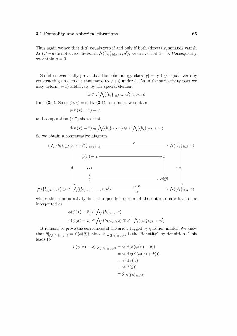
3.1 Formality and spherical fibrations 65
Thus again we see that d(a) equals zero if and only if both (direct) summands vanish.As (z2−u) is not a zero divisor in
∧〈bii∈J , z, u′〉, we derive that a = 0. Consequently,
we obtain a = 0.
So let us eventually prove that the cohomology class [y] = [y + y] equals zero byconstructing an element that maps to y + y under d. As in the surjectivity part wemay deform ψ(x) additively by the special element
x ∈ z′∧〈bii∈J , z, u′〉⊆ kerφ
from (3.5). Since φ ψ = id by (3.4), once more we obtain
φ(ψ(x) + x) = x
and computation (3.7) shows that
d(ψ(x) + x) ∈∧〈bii∈J , z〉 ⊕ z′
∧〈bii∈J , z, u′〉
So we obtain a commutative diagram(∧〈bii∈J , z, z′, u′〉
)|ψ(x)+x
d
φ //∧〈bii∈J , z〉
dE
ψ(x) + x /_
???
x_
y / φ(y)∧
〈bii∈J , z〉 ⊕ z′ ·∧〈bii∈J , . . . , z, u′〉
(id,0)
φ//∧〈bii∈J , z〉
where the commutativity in the upper left corner of the outer square has to beinterpreted as
φ(ψ(x) + x) ∈∧〈bii∈J , z〉
d(ψ(x) + x) ∈∧〈bii∈J , z〉 ⊕ z′ ·
∧〈bii∈J , z, u′〉
It remains to prove the correctness of the arrow tagged by question marks: We knowthat y|∧〈bii∈J ,z〉 = ψ(φ(y)), since φ|∧〈bii∈J ,z〉 is the “identity” by definition. Thisleads to
d(ψ(x) + x)|∧〈bii∈J ,z〉 = ψ(φ(d(ψ(x) + x)))
= ψ(dE(φ(ψ(x) + x)))= ψ(dE(x))= ψ(φ(y))= y|∧〈bii∈J ,z〉
66 3 Rational Homotopy Theory
by the same argument when additionally using the commutativity of the square.The class y is closed by construction, the class d(ψ(x) + x) is closed as it is exact.
Since both classes coincide on the first direct summand, the uniqueness property weproved previously yields
y = d(ψ(x) + x)
So y is exact. Hence we have that [y] = [y] = 0 and that φ∗ is injective.
Step 3. Let us now work with the minimal model(∧
VE , d)
in order to prove for-mality for B. We shall make essential use of the characterisation given in theorem 1.41.So we shall decompose VE as in the theorem, which will yield a similar decompositionfor VB. This will enable us to derive the formality of the minimal model of B. Bytheorem 1.39 this is equivalent to the formality of B itself.
Since E is formal, we may decompose VE = CE ⊕NE with CE = ker dE |VEand N i
E
being a complement of CiE in V iE with the property that every closed element in the
ideal I(NE) generated by NE in∧VE is exact (cf. 1.41).
Without restriction we may assume that there is a subset J ′⊆ J such that
CE = 〈z, bii∈J ′〉(3.9)
where bii∈J , u′ is the homogeneous basis we chose for VB.
We now prove that the morphism
φ :(∧
VB ⊗∧〈z, z′〉, d
)→(∧
VE , dE)
restricts to an isomorphism of commutative differential graded algebras
φ|∧VB:(∧〈bii∈J , u′〉, dB
)→(∧〈z2, bii∈J〉,dE
)Note that clearly d|∧VB
= dB which makes the left hand side a well-defined differentialsubalgebra of the domain of φ. By abuse of notation—the element z2 has word-length2—we write
∧〈z2, bii∈J〉 in order to denote the subalgebra generated by z2, bii∈J
in∧〈z, bii∈J〉.
Foremost we shall see that the morphism is a well-defined and bijective morphismof commutative graded algebras: The right hand side obviously possesses an algebrastructure and a grading as a subalgebra of
∧VE . Moreover, it holds that φ|∧VB
(bi) = bifor i ∈ J and φ|∧VB
(u′) = z2−φ(v) ∈∧〈z2, bii∈J〉, as v ∈
∧〈bii∈J〉. In particular,
we derive that φ|∧VB(u) = z2, which shows that φ|∧VB
is surjective.
3.1 Formality and spherical fibrations 67
It is also injective: Again we may write an arbitrary element a ∈∧〈bii∈J , u′〉 as a
uniquely determined polynomial in u, i.e. a =∑
i bIiui (with the notation introduced
previously). Suppose φ|∧VB(a) = 0 and compute
0 = φ|∧VB(a) = φ|∧VB
(∑i
bIiui
)=∑i
bIi(z2)i
However, the element∑
i bIiz2i ∈
∧VE vanishes if and only if all the bIi equal zero.
Thus we obtain that a = 0.The morphism φ is compatible with differentials (cf. (3.3)). So as soon as we have
identified(∧〈z2, bii∈J〉, dE
)as a differential subalgebra, we have also proved that
φ|∧VBis a morphism of differential algebras. So it remains to see that
∧〈z2, bii∈J〉 is
respected by dE . This, however, is due to the fact that φ|∧VBis surjective, commutes
with differentials (cf. (3.3)) and that(∧
VB, dB)
is a differential algebra. That is, foran element y ∈
∧〈z2, bii∈J〉 there is an element x ∈
(∧VB,dB
)with φ|∧VB
(x) = yand
dE(y) = φ|∧VB(dB(x)) ∈ φ|∧VB
(∧VB)
=∧〈z2, bii∈J〉
This proves that φ|∧VBis an isomorphism of commutative differential graded algebras.
We shall make use of this by constructing a decomposition for VB. We start bysetting
CB := ker dB|VB
In the assertion we assume that the rationalised Hurewicz homomorphismπ∗(B) ⊗ Q −→ H∗(B) is injective in degree n. This guarantees (cf. remark 1.27)that there are no relations in this degree, i.e. V n
B = CnB, which itself implies thatNnE = 0 by construction of
(∧VE , dE
). So every complement of CE in VE necessarily
lies in 〈bii∈J〉. Hence we may assume without restriction that
NE = 〈bii∈J\J ′〉
(For this it might be necessary to change the basis 〈bii∈J〉.) Set
NB := ψ|∧〈bii∈J 〉NE = 〈bii∈J\J ′〉⊆VB
Let us now prove that VB = CB⊕NB and that every closed element in I(NB)⊆∧VB
is exact: Due to (3.9), since φ|∧VBcommutes with differentials (cf. (3.3)) and by our
results on φ|∧VB, we know that 〈bii∈J ′〉⊆ ker dB. Indeed,
dBa =(φ|∧VB
)−1(dE(φ|∧VB(a))) = 0
68 3 Rational Homotopy Theory
for a ∈∧〈bii∈J ′〉.
Moreover, the second (non-technical) assumption asserts that the rationalisedHurewicz homomorphism π∗(B)⊗Q −→ H∗(B) is injective in degree 2n. This againguarantees—cf. 1.27—that V 2n
B = C2nB , which itself implies that u′ ∈ C2n
B , as u′ ∈ V 2nB .
Thus we obtain that 〈bii∈J ′ , u′〉⊆CB. If there was an element 0 6= a ∈ 〈bii∈J\J ′〉with dBa = 0, then dE(φ(a)) = 0, as φ commutes with differentials (cf. (3.3)). However,φ(a) ∈ NE by construction. This yields a contradiction. Hence we really do obtain adirect sum decomposition
VB = CB ⊕NB
with
CB = 〈bii∈J ′ , u′〉 and NB = 〈bii∈J\J ′〉
Now assume there is a closed element y ∈ I(NB). We shall construct an elementx ∈
(∧VB,dB
)with dBx = y. This will finally prove formality in case 1.
The element φ|∧VB(y) ∈
(∧〈z2, bii∈J〉,dE
)equally satisfies dE
(φ|∧VB
(y))
= 0.Moreover, it lies in I(NE): This follows from the fact that φ|∧VB
(bi) = bi for i ∈ Jand that φ is multiplicative. So every monomial with factor bi will be mapped to aproduct with bi as a factor. Every monomial of y contains a factor bI ∈ NB. Henceevery factor of φ|∧VB
(y) contains the factor bI ∈ NE and φ|∧VB(y) ∈ I(NE).
Thus by formality of E there is an element x ∈(∧
VE , dE)
with dEx = φ|∧VB(y).
As x ∈(∧
VE ,dE), we may write
x = x0 + x1z + x2z2 + x3z
3 + . . .
as a finite sum with xi ∈∧〈bii∈J〉. Since z is dE-closed, we compute
〈z2, bii∈J〉⊇φ|∧VB(y) = dE(x) = dE(x0) + dE(x1)z + dE(x2)z2 + . . .
As(∧〈z2, bii∈J〉,dE
)is a differential subalgebra of
(∧VE , dE
), we see that a term
dE(xi)zi lies in zi ·∧〈z2, bii∈J〉 again. In particular, the parity of the power of z is
preserved by differentiation. Thus—by comparison of coefficients in z—we obtain∑i≥0
dE(x2i+1) = 0
In particular, we see that already
dE(x0 + x2z2 + x4z
4 + . . . ) = φ|∧VB(y)
Hence, without restriction, we may assume x to consist of monomials with even powersof z only, i.e. x2i+1 = 0 for i ≥ 0. Thus it holds that x ∈ 〈z2, bii∈J〉. As φ|∧VB
is
3.1 Formality and spherical fibrations 69
bijective, there is the well-defined element x =(φ|∧VB
)−1(x) ∈∧VB . As φ commutes
with differentials (cf. (3.3)), we eventually obtain
dB(x) =(φ|∧VB
)−1(dE(x)) =(φ|∧VB
)−1(φ|∧VB
(y))
= y
Case 2. We shall now prove the assertion under the assumption that the fibrationis non-primitive. Again we shall rely on the quasi-isomorphism(∧
VB ⊗∧〈z, z′〉, d
) '−→ (APL(E), d)
where the left hand side contains the minimal Sullivan algebra(∧
VB, dB)
as adifferential subalgebra. Again this last algebra is supposed to be a minimal model forthe space B.
Step 1. We show that the algebra generated by VE := VB ⊕ 〈z, z′〉 is a minimalSullivan algebra: We have ∧
VB ⊗∧〈z, z′〉 =
∧VE
Set dE := d. So(∧
VE , dE)
is a commutative differential graded algebra. Moreover,it holds that V 1
E = 0, since B is simply-connected by assumption.By the definition of (non-)primitivity u ∈
∧VB is decomposable, i.e.
u ∈∧>0 VB ·
∧>0 VB. Thus we have that dEz′ = z2 − u ∈∧>0 VE ·
∧>0 VE .Clearly, dEz = dEu = 0 and dEbi ∈
∧>0 VB ·∧>0 VB for i ∈ J , as
(∧VB,dB
)is a minimal differential subalgebra of
(∧VE , dE
). As dE is a derivation, we obtain
im dE ∈∧>0 VE ·
∧>0 VE .These properties taken together with proposition 1.25 yield that
(∧VE , dE
)is a
minimal Sullivan model of E.
Step 2. By assumption E is formal. Theorem 1.41 then yields the existence of adecomposition VE = CE ⊕ NE with CE = ker dE |VE
. Clearly, we have z ∈ CE andwithout restriction we may assume that
CE = 〈z, bii∈J ′〉
for a subset J ′⊆ J , where bii∈J now is a homogeneous basis of VB. (Recall thatnon-primitivity implies that the element u lies in
∧≥2〈bii∈J〉.)
Since dEz′ 6= 0 and since z′ ∈ VE , there is an element c ∈ C with the property thatz′ + c ∈ NE . Set z′ := z′ + c. Thus we have that z′ ∈ NE . The change of basis causedby z′ 7→ z′ induces a linear automorphism of the vector space VE which is the identity
70 3 Rational Homotopy Theory
on VB⊕〈z〉. This automorphism itself induces an automorphism σ of the commutativedifferential graded algebra
∧VE . By construction this automorphism has the property
that σ|∧(VB⊕〈z〉) = id. Moreover, we know that dE(∧
(VB ⊕ 〈z〉))⊆∧
(VB ⊕ 〈z〉).Therefore σ is also compatible with the differential, since
dE(σ(x)) = σ(dE(x)) for x ∈∧
(VB ⊕ 〈z〉)
dE(σ(z′)) = dE(z′) = dE(z′ + c) = dE(z′) = z2 − u = σ(z2 − u) = σ(dE(z′))
Thus up to this isomorphism of differential graded algebras we may assume thatthere is a decomposition of VE = CE ⊕NE with CE = ker dE |VE
and with z′ ∈ NE .Moreover, up to a change of basis we hence may assume that
NE = 〈bii∈J\J ′ , z′〉
We use this to split VB in the following way: Set CB := ker dB|VB. We recall that(∧
VB,dB)
is a differential subalgebra of(∧
VE , dE). Thus we realise that
CB = 〈bii∈J ′〉
and we set
NB : = 〈bii∈J\J ′〉
We directly obtain VB = CB ⊕NB.As for formality of B, by theorem 1.41 it remains to prove that every closed element
in the ideal I(NB) generated by NB in(∧
VB,dB)
is exact in(∧
VB,dB). So let
y ∈ I(NB) with dBy = 0. Since NB ⊆NE we obtain that I(NB)⊆ I(NE). Thus bythe formality of E we find an element x ∈
∧VE with dEx = y. Recall the notation we
introduced in the surjectivity part of case 1, step 2 and write x as a finite sum
x = bI0 + bI1z + bI2z2 + · · ·+ bI′0z
′ + bI′1zz′ + bI′2z
2z′ + . . .
with bIi , bI′i ∈∧VB. We compute
y = dEx =dEbI0 + (dEbI1)z + (dEbI2)z2 + . . .
+((dEbI′0)z′ + bI′0
(z2 − u))
+((dEbI′1)zz′ + bI′1
z(z2 − u))
+((dEbI′2)z2z′ + bI′2
z2(z2 − u))
+ . . .(3.10)
=∑i≥0
((dEbIi)− bI′iu+ bI′i−2
)zi +
∑i≥0
(dEbI′i)z′zi
Since dE(bi) ∈∧VB for 1 ≤ i ≤ m and since u ∈
∧VB, we shall proceed with our
reasoning by comparing coefficients in zi respectively in z′zi. That is, the element y
3.1 Formality and spherical fibrations 71
lies in∧VB. Thus it cannot contain a summand with zi (for i > 0) or with z′zi (for
i ≥ 0) as a factor. So we see that
y = dEx = dEbI0 − bI′0u
In particular, (dEbI2)− bI′2u+ bI′0= 0. Thus the element bI0 + bI2u ∈
∧VB satisfies
dE(bI0 + bI2u) = dEbI0 +(dEbI2
)u = dEbI0 + bI′2
u2 − bI′0u = y + bI′2u2
Below we prove that bI′2 is exact, i.e. there is some a ∈∧VB with dEa = bI′2
. Thisyields the exactness of bI′2u
2 by dE(au2) = bI′2u2. So we finally shall obtain
dE(bI0 + bI2u− au2) =(y + bI′2
u2)− bI′2u
2 = y
Since this is a computation in∧VB and since dE restricts to dB on
∧VB we obtain
that y is exact in∧VB. This will provide formality.
So let us finally prove that bI′2 is exact. Since we are dealing with finite sums only,there is an even i0 ≥ 2 with bI′i0
= 0. From (3.10) we again see that
0 = (dEbIi0 )− bI′i0u+ bI′i0−2
= (dEbIi0 ) + bI′i0−2
This implies dB(−bIi0 ) = bI′i0−2and bI′i0−2
is exact in(∧
VB, dB). We shall continue
this iteratively. That is, as a next step we have
0 = (dEbIi0−2)− bI′i0−2u+ bI′i0−4
= (dEbIi0−2)− dB(− bIi0
)+ bI′i0−4
and bI′i0−4is dB-exact. As i0 is even, this iterative procedure will finally end up with
proving that bI′2 is exact.This finishes the proof of the formality of B.
We already did so in the proof and we shall continue to do so: We refer to the twoconditions in the assertion of the theorem that involve the Hurewicz homomorphismas “non-technical” conditions. (The other prerequisites are mainly due to the generalsetting of the theory.)
It is of importance to remark that S2n (n ≥ 1) is an F0-space. Thus the questionwhether formality of the base space implies formality for the total space is relatedto the Halperin conjecture—cf. [56] for an introduction to this topic and theorem[56].3.4 in particular. The Halperin conjecture has been established on these spheres.
72 3 Rational Homotopy Theory
Reformulations (cf. [58]) of the conjecture permit extremely short proofs for this. Forexample it is trivial to see that the cohomology algebra H∗(S2n) does not admit non-trivial derivations of negative degree. A direct proof needs to show that every sphericalfibration with fibre of even rational homological dimension is totally non-cohomologousto zero, i.e. that the Serre spectral sequence degenerates at the E2-term; respectivelythat the inclusion of the fibre into the total space induces a surjective map in rationalcohomology. For this see remark 1.34.
A consequence of theorem [56].3.4 now is that if the fibre of a fibration is an F0-space, then the formality of the base space implies the formality of the total space. Inparticular, this proves
Theorem 3.3. Let
F → Ep−→ B
be a spherical fibration of simply-connected (and path-connected) topological spaces.Let the fibre satisfy F 'Q Sn for an even n ≥ 2.
Then it holds: If B is a formal space, then so is E.
Nonetheless, we shall give a direct proof of this theorem, as this proof will providesome observations and tools which we shall need in the following.
Proof of Theorem 3.3. Choose a minimal model
mB :(∧
VB,dB) '−→ (APL(B),d)
As B is formal we have the quasi-isomorphism
µB :(∧
VB,dB) '−→ (H∗(B), 0)
from lemma 1.44. For this we fix a complement N of ker d|VBin VB. We obtain that
µB(N)=0. Form the model of the fibration p
mE :(∧
VB ⊗∧〈z, z′〉,d
) '−→ (APL(E), d)
as in remark 1.34. We use the terminology of theorem 3.2 for the model of the fibration,i.e. d(z′) = u ∈
∧VB and bii∈J denotes a homogeneous basis of VB. (Here we do
not make use of a distinguished basis element u′.) We now define a morphism ofcommutative graded algebras
µE :(∧
VB ⊗∧〈z, z′〉, d
)→ (H∗(E), 0) ∼= (H∗(B)⊕H∗(B) · [z], 0)
bi 7→ µB(bi)z 7→ [z](3.11)z′ 7→ 0
3.1 Formality and spherical fibrations 73
by extending this assignement linearly and multiplicatively. We shall prove that thismorphism of commutative graded algebras is actually a quasi-isomorphism. The weakequivalence
(APL(E),d) mE←−−(∧
VB ⊗∧〈z, z′〉, d
) µE−−→ (H∗(E), 0)
will then yield the formality of E.
Our main tool for proving this will be that every closed element of(∧VB ⊗
∧〈z, z′〉, d
)maps to its homology class under µE . Let us establish this
result first. So suppose
y ∈(∧
VB ⊗∧〈z, z′〉, d
)is such a d-closed element. It then may be written as
y = y0 + z′y1
with y0, y1 ∈∧(
VB ⊕ 〈z〉).
First we shall prove that y1 is exact. We have
0 = dy = dy0 + (z2 − u)y1 − z′dy1
By construction of(∧
VB ⊗∧〈z, z′〉,d
)we know that
d(∧
VB ⊕ 〈z〉)⊆(∧
VB ⊕ 〈z〉)
This implies that dy1 = 0. Thus we have
dy0 = −(z2 − u)y1(3.12)
Hence we write
y0 = y0,0 + y0,1z + y0,2z2 + y0,3z
3 + · · ·+ y0,kzk
and
y1 = y1,0 + y1,1z + y1,2z2 + y1,3z
3 + · · ·+ y1,k−2zk−2
as z-graded elements with y0,i, y1,i ∈∧VB. As z is d-closed, the grading is preserved
under differentiation. Equation (3.12) implies in this graded setting that
dBy0,i = uy1,i − y1,i−2
74 3 Rational Homotopy Theory
Starting in top degree k we see that dBy0,k = −y1,k−2. Set xk−2 := −y0,k. Thisdirectly leads to
dBy0,k−2 = uy1,k−2 − y1,k−4
where uy1,k−2 is dB-exact by dB(−uy0,k) = uy1,k−2. Thus y1,k−4 is exact. Set
xk−4 := −y0,k−2 − uy0,k
Hence, inductively continuing in this fashion, we obtain that each y1,i with i ≡ kmod 2 is exact. The same line of argument applied from degree k − 1 downwardsyields finally that also all the y1,i with i ≡ k − 1 mod 2 are dB-exact. In total, foreach 0 ≤ i ≤ k − 2 there exists an xi ∈
∧VB with dxi = y1,i. So the element y1 itself
is exact: Set
x : = x0 + x1z + x2z2 + · · ·+ xk−2z
k−2
and obtain
d(x) = d(x0 + x1z + x2z
2 + · · ·+ xk−2zk−2)
= dBx0 + dB(x1)z + dB(x2)z2 + · · ·+ dB(xk−2)zk−2(3.13)
= y1,0 + y1,1z + y1,2z2 + y1,3z
3 + · · ·+ y1,k−2zk−2
= y1
Moreover, the xi are constructed iteratively within the algebra∧VB. So we obtain
xi ∈∧VB for 0 ≤ i ≤ k − 2 and
x ∈∧
(VB ⊕ 〈z〉)(3.14)
This will enable us to see that y is mapped to its homology class. Due to theformality of B we may decompose VB = C ⊕N homogeneously with the property thatC = ker dB|V and such that every closed element in I(N), the ideal generated by Nin∧VB, is exact—cf. theorem 1.41. This complement N is supposed to be identical
to the one we chose for defining µB at the beginning of the proof. This decompositioninduces a decomposition ∧
VB =∧C ⊕ I(N)
For each 1 ≤ i ≤ k we split y0,i =: y′0,i + y′′0,i with y′0,i ∈∧C (being d-closed) and
y′′0,i ∈ I(N). The morphism µB was chosen to map a closed element to its homology
3.1 Formality and spherical fibrations 75
class and to vanish on I(N)—cf. lemma 1.44. Thus we see that µE(y′0,i) = [y′0,i] andthat µE(y′′0,i) = 0. We then need to show that
µE(y) =∑i≥0
[y′0,i][z]i != [y]
This will be a consequence of the following reasoning: We suppose y0,i = y′′0,i for all0 ≤ i ≤ k and show that
µE(y) = [0] != [y]
By construction we have
y0 ∈ N ·∧
(V ⊕ 〈z〉)(3.15)
We shall now show that the element
y + d(z′x) = y0 + z′y1 + (z2 − u)x− z′y1 = y0 + (z2 − u)x
is exact, which will imply the exactness of y itself.The whole commutative algebra splits as a direct sum∧
VB ⊗∧〈z, z′〉 =
(∧(C ⊕ 〈z〉)
)⊕(
(N ⊕ 〈z′〉) ·(∧
VB ⊗∧〈z, z′〉
))Thus the element x may be written as x = c + n with c ∈
∧(C ⊕ 〈z〉) and
n ∈ (N ⊕ 〈z′〉) ·(∧
VB ⊗∧〈z, z′〉
). We conclude that d(c) = 0 and that d(x − c) =
dn = dx. Hence, without restriction, we may assume x = n. Combining this with(3.14) thus yields
x ∈ N ·∧(
VB ⊕ 〈z〉)
Thus, writing x in its z-graded form, we see that each coefficient xi (for 0 ≤ i ≤ i− 2)lies in I(N) = N ·
∧VB. By (3.15) every coefficient y0,i (for 0 ≤ i ≤ k) in the z-grading
of y0 equally lies in I(N). Hence so does every z-coefficient
y0,i − uxi + xi−2 ∈ I(N)
of
y0 + (z2 − u)x =∑i≥0
(y0,i − uxi + xi−2)zi
Since y was assumed to be d-closed and since y0 + (z2 − u)x = y + d(z′x), the elementy0 + (z2 − i)x also is d-closed. In particular, every z-coefficient is a dB-closed element
76 3 Rational Homotopy Theory
in I(B). By the formality of B and by theorem 1.41 every such coefficient is dB-exactthen. An analogous argument to (3.13) then shows that y is d-exact. In total, thisproves that µ maps a closed element to its cohomology class.
As for the properties of µE , which now follow easily from this feature, we observe:The morphism is compatible with differentials as µ(d(x)) = 0. (The closed and exactclass d(x) maps to its cohomology class.) Eventually, it is a quasi-isomorphism as themorphism induced in homology is just the identity. This proves formality for E.
We remark that making extensive use of theorem 1.41 permits a shorter but similarproof. Yet, for us it was important to establish the quasi-isomorphism (3.11). Indeed,it will be a vital tool in the next theorem.
As we have seen, it becomes pretty clear that the formality of the base space andthe formality of the total space are highly interconnected. This is illustrated oncemore by the next theorem.
Theorem 3.4. Let
F → Ep−→ B
be a spherical fibration of simply-connected (and path-connected) topological spaces.Let the fibre satisfy F 'Q Sn for an even n ≥ 2.
If B and (consequently) E are formal spaces, then the fibration p is a formal map.
Proof. We shall use the terminology and results from theorem 3.2. By
mB :(∧
VB, dB) '−→ APL(B, d)
we denote the minimal model. We let bii∈J denote a basis of VB (and do not makeuse of a distinguished element u′).
Case 1. Suppose the fibration p to be primitive. In the notation of theorem 3.2we then have dz′ = z2 − u with primitive u in the model of the fibration. In the caseu = 0 we obtained the weak equivalence
E 'Q B × F
and we have seen the model of the fibration to be just the product model of fibre andbase. The diagram
APL(B)APL(p) // APL(E) ∼= (APL(B), d)⊗ (APL(F ), d)
(∧VB, dB
) x 7→(x,1) //
'
OO
(∧VB, dB
)⊗(∧
VF , dF)'
OO
3.1 Formality and spherical fibrations 77
commutes (cf. [22], p. 198), where(∧
VF ,dF)
is the minimal model of the fibre F . Soalso the induced map APL(p) is just the canonical inclusion into the first factor. Thustheorem 1.47 applies and yields the formality of p in this case.
So we may assume u 6= 0. We then have constructed the minimal model
mE :(∧
VE ,dE) '−→ APL(E,d)
in case 1, step 2 of theorem 3.2. By lemma 1.38 we have a quasi-isomorphism
µB :(∧
VB,dB) '−→ (H∗(B), 0)
which we may assume to satisfy (mB)∗ = (µB)∗. Once more, for a spherical fibrationwe form the model of the fibration
mE :(∧
VB ⊗∧〈z, z′〉, d
) '−→ (APL(E), d)
in the altered version of remark 1.34. Consider the following diagram(∧VE ,dE
)
mE
ww
(∧VB,dB
)p
00
//
mB
(∧VB ⊗
∧〈z, z′〉,d
)φ66lllllllllllll
mE
(APL(B), d)
APL(p) // (APL(E),d)
(3.16)
where φ is the quasi-isomorphism from (3.2), which we construct in the proof oftheorem 3.2, case 1, step 2. (Note that until case 1, step 3 of the theorem we didnot need any of the “non-technical” assumptions which we did not require for thistheorem.)
We shall now prove that diagram (3.16) commutes up to homotopy. The minimalmodel mE was constructed by means of a diagram of liftings and isomorphismsextending
(APL(E), d) mE←−−(∧
VB ⊗∧〈z, z′〉, d
) φ−→(∧
VE , dE)
(cf. the proof of lemma 1.38). Thus this diagram is commutative up to homotopy(cf. [22].12.9, p. 153) and so is the right hand triangle of (3.16).
78 3 Rational Homotopy Theory
Since the model of the fibration comes out of a relative Sullivan algebra(cf. [22].14 and [22].15, p. 196) for APL(p)—composed with the minimal model(∧
VB,dB) mB−−→ APL(B, d)—the algebra
(∧VB,dB) includes into
(∧VB⊗
∧〈z, z′〉, d
)by x 7→ (x, 1) as a differential subalgebra (cf. definition [22], p. 181) and the square inthe diagram commutes. (This holds although we altered the model of the fibration asin remark 1.34.)
As a consequence, both the following diagrams commute up to homotopy—thesecond one as the Sullivan representative p is constructed as a lifting (cf. section 1.2).
(∧VB, dB
) φ|∧ VB //
mB
(∧VE ,dE
)mE
(APL(B), d)
APL(p)// (APL(E), d)
(∧VB,dB
) p //
mB
(∧VE , dE
)mE
(APL(B),d)
APL(p)// (APL(E),d)
Since the Sullivan representative p is uniquely defined up to homotopy, we know thatp and φ|∧VB
are homotopic morphisms (cf. [22], p. 149). Thus—in order to prove theassertion in this case—it is sufficient to find a minimal model µE with (µE)∗ = (mE)∗for which the diagram
(∧VB, dB
) φ|∧ VB //
µB
(∧VE ,dE
)µE
(H∗(B), 0)
p∗ // (H∗(E), 0)
commutes up to homotopy.We shall start to do so by foremost recalling the quasi-isomorphism
µE :(∧
VB ⊗∧〈z, z′〉, d
) '−→ (H∗(E), 0)
bi 7→ µB(bi)z 7→ [z]z′ 7→ 0
from (3.11). (See the rest of the proof of theorem 3.3 for the fact that this reallydefines a quasi-isomorphism.) For the definition of the morphism and in the followingwe shall identify H∗(E) with p∗H∗(B) ⊕ p∗H∗(B)[z]. Note that this morphism hasthe property that (µE)∗ = (mE)∗. This can be derived as follows: We assumed theanalogous property to hold true for µB. Moreover, we have
(mE)∗ = ((mB)∗, (mB)∗) : H∗(B)⊕H∗(B)[z]∼=−→ H∗(E)
by the construction of the model of the fibration as a relative Sullivan model over thebasis
(∧VB,dB
). This, however, coincides with the definition of (µE)∗.
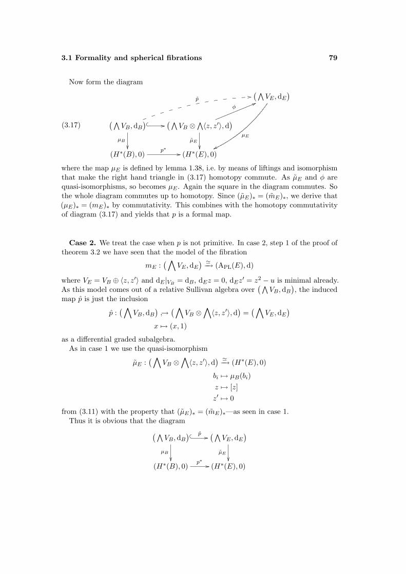
3.1 Formality and spherical fibrations 79
Now form the diagram (∧VE ,dE
)
µE
ww
(∧VB,dB
)p
00
k j i h g f f e d c b a
//
µB
(∧VB ⊗
∧〈z, z′〉,d
)φ66lllllllllllll
µE
(H∗(B), 0)
p∗ // (H∗(E), 0)
(3.17)
where the map µE is defined by lemma 1.38, i.e. by means of liftings and isomorphismthat make the right hand triangle in (3.17) homotopy commute. As µE and φ arequasi-isomorphisms, so becomes µE . Again the square in the diagram commutes. Sothe whole diagram commutes up to homotopy. Since (µE)∗ = (mE)∗, we derive that(µE)∗ = (mE)∗ by commutativity. This combines with the homotopy commutativityof diagram (3.17) and yields that p is a formal map.
Case 2. We treat the case when p is not primitive. In case 2, step 1 of the proof oftheorem 3.2 we have seen that the model of the fibration
mE :(∧
VE , dE) '−→ (APL(E),d)
where VE = VB ⊕ 〈z, z′〉 and dE |VB= dB, dEz = 0, dEz′ = z2 − u is minimal already.
As this model comes out of a relative Sullivan algebra over(∧
VB,dB), the induced
map p is just the inclusion
p :(∧
VB, dB)→(∧
VB ⊗∧〈z, z′〉, d
)=(∧
VE ,dE)
x 7→ (x, 1)
as a differential graded subalgebra.As in case 1 we use the quasi-isomorphism
µE :(∧
VB ⊗∧〈z, z′〉,d
) '−→ (H∗(E), 0)
bi 7→ µB(bi)z 7→ [z]z′ 7→ 0
from (3.11) with the property that (µE)∗ = (mE)∗—as seen in case 1.Thus it is obvious that the diagram(∧
VB, dB) p //
µB
(∧VE , dE
)µE
(H∗(B), 0)
p∗ // (H∗(E), 0)
80 3 Rational Homotopy Theory
commutes. So p is formal in this case, too.
We shall now state some results related to the previous theorems. We begin withthe following apparent consequence:
Corollary 3.5. Let
F → Ep−→ B
be a spherical fibration of simply-connected (and path-connected) topological spaceswith rational homology of finite type. Let the fibre satisfy F 'Q Sn for an even n ≥ 2.Suppose further that the space B is rationally (2n− 1)-connected.
Then we derive:
• The space E is formal if and only if so is B.
• If this is the case, the map p is formal, too.
Proof. Since B is rationally (2n− 1)-connected, we have
πi(B)⊗Q = 0 = H i(B) for i ≤ 2n− 1
So we obtain in particular that the rationalised Hurewicz homomorphismπ∗(B) ⊗ Q −→ H∗(B) is injective in degree n. By the Hurewicz theorem we alsoobtain that the rationalised Hurewicz homomorphism π∗(B) ⊗ Q −→ H∗(B) is anisomorphism in degree 2n—and injective in this degree, in particular. (We may realisethis directly by building the minimal model
(∧VB, dB
)of B, which has the property
that V ≤2n−1 = 0. As the model is minimal, every element in V 2n is closed andH2n(B) ∼= H2n(B) = V 2n ∼= π2n(B)⊗Q by the Hurewicz homomorphism—cf. remark1.27.)
Thus all the prerequisites of theorem 3.2 are satisfied and the formality of E impliesthe one of B. By theorem 3.3 we have the reverse implication and theorem 3.4 finishesthe proof.
We remark that this corollary only needs case 1 of theorem 3.2, since by theconnectivity-assumption the fibration necessarily is primitve.
Let us formulate an observation from the proofs of the different theorems in thischapter.
Theorem 3.6. Let
F → Ep−→ B
3.1 Formality and spherical fibrations 81
be a fibration of simply-connected (and path-connected) topological spaces with rationalhomology of finite type. Suppose the rational cohomology algebra H∗(F ) is generated(as an algebra) by exactly one (non-trivial) element of even degree n. Suppose furtherthat the space B is rationally n′-connected, where
n′ := n · (dimQH∗(F ))− 1
Then we obtain: The space E is formal if and only if so is B. In this case the mapp is formal, too.
Proof. Set d := dimQH∗(F ). The cohomology algebra of the fibre F is given by
the polynomial algebra H∗(F ) = Q[z]/zd. The minimal model(∧
VF ,dF)
of F isgiven by VF = V n ⊕ V n·d−1 with V n = 〈z〉 and V n·d−1 = 〈z′〉 and by the differentialsdF z = 0 and dF z′ = zd. See example 1.32 for details.
Let(∧
VB,dB)
be a minimal model of the base space B. We form the model of thefibration: (∧
VB ⊗∧VF , d
) '−→ (APL(E),d)
The differential d of the model equals dB on the subalgebra∧VB. It remains to
describe the differentials d(z) and d(z′). As B is n′-connected, we obtain V ≤n′
= 0.Thus, due to theorem 1.21, we derive that dz = dF z = 0 and dz′ = dF z′ = zd − u forsome u ∈ V d·n
B . As(∧
VB,dB)
is minimal and since V <d·n = 0, we necessarily obtaindu = dBu = 0.
The result now follows by imitating the proofs of theorems 3.2, 3.3 and 3.4 in acompletely analogous fashion. Just replace z2 by zd and adapt the calculations. Someiterative constructions will need to be done not only on even and odd indices separately,but for each class modulo d. In theorem 3.2 clearly only case 1 has to be considered.Neither are new ideas required nor has there any essential change to be made tothe proofs. As we have already seen in the proof of corollary 3.5 the connectednessassumption is sufficient to derive all the “non-technical” conditions in theorem 3.2.This combines to yield the result.
A crucial example enters the stage: This theorem directly applies to fibrations withfibre F having the rational homotopy type of either CPn or HPn—always supposedthat all the other assumptions (including the connectivity-assumption) are fulfilled.In such a case the cohomology ring is given by H∗(F ) = Q[z]/zn+1 with deg z = 2 ordeg z = 4 respectively. This leads us to
Remark 3.7. Let E → M be a complex vector bundle of rank n over a simply-connected smooth (closed) manifold M . Let
CPn−1 → PC(E)p−→M
82 3 Rational Homotopy Theory
be the associated fibre-wise complex projectivisation. By the Hirsch lemma we obtainthe isomorphism of H∗(M)-modules H∗(PC(E)) ∼= H∗(M)⊗H∗(CPn−1) which forcesthe cohomology algebra to be of the form
H∗(PC(E)) ∼= H∗(M)[z]/(zn + c1(E)zn−1 + · · ·+ cn(E))
for certain coefficients, the Chern classes, ci(E) (for 1 ≤ i ≤ n). The Chern classesidentify with the cohomology classes of the obstructions ui which we obtain in themodel of the fibration:
dz′ = zn + u1zn−1 + · · ·+ un
where(∧〈z, z′〉,d
)denotes a minimal model for CPn−1. So for example a vanishing
of the Chern classes ci(E) for 1 ≤ i ≤ n − 1 yields a situation similar in nature towhat we dealt with.
Note that unit sphere bundles associated to real vector bundles over a manifoldprovide another class of examples to which theorems 3.2, 3.3 and 3.4 may be applicable.The cohomology class [u] of the obstruction u in the differential dz′ = z2 − u we usedthroughout the proofs of the theorems again may be linked to the characteristic classesof the real vector bundle itself (cf. example [22].15.4, p. 202).
The following proposition is a specialised version of theorem 3.2.
Proposition 3.8. Let
F → Ep−→ B
be a spherical fibration of simply-connected (and path-connected) topological spaceswith rational homology of finite type. Let the fibre satisfy F 'Q Sn for an even n ≥ 2.Suppose further that the rationalised Hurewicz homomorphism π∗(B)⊗Q −→ H∗(B)is injective in degree n. Additionally assume the space B to be k-connected with3k + 2 ≥ 2n.
Then we obtain: If the space E is formal, so is B.
Proof. In order to be able to apply theorem 3.2 we need to slightly modify itsproof: In case 1, step 3 we used that the rationalised Hurewicz homomorphism wassupposed to be injective in degree 2n. The purpose of this assumption was to showthat V 2n
B = C2nB or actually merely that u′ ∈ C2n
B .We know that dz′ = z2− u with u− u′ ∈
∧≥2〈bii∈J〉 in the model of the fibration(cf. 1.34) and with u being dB-closed. We have to show that our new condition is aptto replace the former one, i.e. to equally yield u′ ∈ C2n
B .Since B is k-connected, it holds that V ≤kB = 0. Moreover, this also leads to
dBV ≤2k = 0 by the minimality of(∧
VB,dB). As (2k + 1) + (k + 1) = 3k + 2, this
3.1 Formality and spherical fibrations 83
itself implies that
dB
((∧≥2VB
)≤3k+2)= 0
Thus by the assumption 3k + 2 ≥ 2n we derive that the element u− u′ ∈(∧
V ≥2)2n
is closed, i.e. dB(u − u′) = 0. However, we know that dBu = 0, whence dBu′ = 0and u′ ∈ C2n
B . From here the proof of the theorem can be continued without anychange.
The connectedness-assumption of the proposition is automatically satisfied ifF 'Q S2. So we may formulate very catchy special versions of the proposition:
Corollary 3.9. Let
S2 → Zp−→M
be a fibre bundle of simply-connected smooth closed manifolds.Then we obtain:
• If Z is formal, so is M .
• If Z is a complex manifold satisfying the ddc-lemma, then M is formal.
Proof. Smooth manifolds have (rational) homology of finite type. In the terminologyof proposition 3.8 we have n = 2 and k = 1, since M is simply-connected. Sothe condition 5 = 3k + 2 ≥ 2n = 4 is satisfied. A model
(∧V,d
)of a simply-
connected space X satisfies dV 2 = 0 and H2(X) ∼= V 2 if it is minimal. We identifyV 2M∼= Hom(π2(M),Q) and H2(M) ∼= Hom(H2(M),Q) by universal coefficients. By
remark 1.27 this amounts to the fact that the rationalised Hurewicz homomorphismfor M is given by an isomorphism
V 2M∼= πn(M)⊗Q
∼=−→ H∗(M) ∼= V 2M
(Clearly, we just could have cited the Hurewicz theorem once more.) In particular, itis injective. Now proposition 3.8 applies. If Z is complex satisfying the ddc-lemma,then it is formal—cf. lemma 1.37 and the reasoning below it.
This leads us to the main geometric result:
Theorem 3.10. A Positive Quaternion Kahler Manifold is a formal space. Thetwistor fibration is a formal map.
84 3 Rational Homotopy Theory
We shall give two slightly different proofs of the theorem. The first one basicallyrelies on the recognition theorem for the complex Grassmannian (cf. 1.12); the secondone will need clearly less structure theory of Positive Quaternion Kahler Geometry. Itis not surprising that both proofs make essential use of the twistor fibration.
First proof of theorem 3.10. For every Positive Quaternion Kahler ManifoldM there is the twistor fibration
S2 → Z →M(3.18)
with Z a compact Kahler manifold. Positive Quaternion Kahler Manifolds are simply-connected. Thus so is Z. (As compact manifolds both M and Z have finite-dimensional(rational) homology.) The twistor space Z is a compact Kahler manifold (cf. theorem1.8) so that it satisfies the ddc-lemma. Thus Z is a formal space.
Positive Quaternion Kahler Manifolds have vanishing odd-degree Betti numbers, i.e.b2i+1(M) = 0 (for i ≥ 0)—cf. theorem 1.13. In particular, b3(M) = 0.
A Positive Quaternion Kahler Manifold Mn satisfying b2(M) > 0 is necessarilyisometric to the complex Grassmannian Gr2(Cn+2)—cf. corollary 1.12. The latteris a symmetric space. Consequently, it is formal (cf. example 1.36). Thus, withoutrestriction, we may focus on the case when b2(M) = 0.
In total, we may assume M to be rationally 3-connected. Now corollary 3.5 appliesand yields the formality of M . So both M and Z are formal and theorem 3.4 tells usthat the twistor fibration is a formal map.
Second proof of theorem 3.10. As in the first proof we use the twistor fibra-tion (3.18) and apply corollary 3.9 to it. Since Z is a formal space, the corollarydirectly yields the result.
Note that we do not use b2(M) = b3(M) = 0 in the second proof!Needless to mention that formality may be interpreted as some sort of rigidity result:
Whenever M has the rational cohomology type of a Wolf space, it also has the rationalhomotopy type of the latter.
For the definition of the following numerical invariants see the definition on [22].28,p. 370, which itself relies on various definitions on the pages 351, 360 and 366 in[22].27.
Corollary 3.11. A rationally 3-connected Positive Quaternion Kahler Manifold Msatisfies
dimM
4= c0(M) = e0(M) = cat0(M) = cl0(M)
3.1 Formality and spherical fibrations 85
Proof. On a Positive Quaternion Kahler Manifold Mn there is a class u ∈ H4(M)with respect to which M satisfies the analogue of the Hard-Lefschetz theorem (cf. theo-rem 1.13). In particular, there is the volume form un 6= 0. Thus the rational cup-lengthof a rationally 3-connected Positive Quaternion Kahler Manifold M is c0(M) = dimM
4 .The rest of the equalities is due to formality (cf. [22], example 29.4, p. 388).
Clearly, Positive Quaternion Kahler Manifolds are necessarily simply-connected andcompact. This leads to
Corollary 3.12. A compact simply-connected Non-Negative Quaternion Kahler Man-ifold is a formal space. The twistor fibration is formal.
Proof. Quaternion Kahler Manifolds are Einstein and therefore can be distinguishedby their scalar curvature being positive, zero or negative. The case of positive scalarcurvature now follows from theorem 3.10. A simply-connected Quaternion KahlerManifold with vanishing scalar curvature is hyperKahlerian and Kahlerian in particular.So it is a formal space. The twistor fibration in this case is the canonical projectionM × S2 →M .
Let us end this section by presenting some vague ideas and speculations that arerather thought of as a motivation for the reader to get involved in the subject than tobe a sound outline of what is possible.
Before we do so we shall hint to the fact that the question of formality is a prominentand recurring topic in the field of special geometries (like G2-holonomy).
Let us venture to give a daring interpretation of the formality of Positive QuaternionKahler Manifolds: The Bott conjecture speculates that simply-connected compactRiemannian manifolds with non-negative sectional curvature are rationally elliptic. Inthe quaternionic setting theorems as the connectivity lemma (cf. theorem A on [19],p. 150) might suggest that scalar curvature could be seen as an adequate conceptualsubstitute for sectional curvature. (The only Positive Quaternion Kahler Manifoldwith positive sectional curvature is HPn.) Furthermore, we know that the sectionalcurvature “along a quaternionic plane” is positive (cf. formula [5].14.42b, p. 406),which again relates quaternionic geometry to positive sectional curvature.
In the case of Positive Quaternion Kahler Manifolds—mainly because rationalcohomology is concentrated in even degrees only—we suggest to see formality as avery weak substitute for ellipticity: In the rational elliptic case, we are dealing withF0-spaces, which admit pure models. Thus the images of the relations—the odd degreegenerators of the vector space underlying the minimal model— under the differentialin the minimal model are very well-behaved as they correspond to a regular sequence.In particular, there are no algebraic combinations of these images that correspond tonon-vanishing cohomology classes.
86 3 Rational Homotopy Theory
In the case of formality we do not necessarily have this regularity of these images.However, the very effect in cohomology is enforced by an additional generator of theminimal model—corresponding to a homotopy group—which is supposed to map tosuch a non-trivial algebraic combination under the differential. The effect in cohomologythen clearly is the same: The cohomology class of the algebraic combination is zero.
If one is willing to engage with this point of view, the formality of Positive QuaternionKahler Manifolds might be seen as heading towards a quaternionic Bott conjecture.
There is a notion of geometric formality introduced by Kotschick (cf. [49]) consistsin the property that the product of harmonic forms is harmonic again. Geometricformality enforces strong restrictions on the topological structure of the underlyingmanifold. For example, the Betti numbers of the manifold Mn are restricted fromabove by the Betti numbers of the n-dimensional torus—cf. [49], theorem 6. Thisresult was even improved on Kahler manifolds by Nagy—cf. [62], corollary 4.1.
Symmetric spaces are geometrically formal (cf. [50], [71]). Thus it is tempting toconjecture the same for Positive Quaternion Kahler Manifolds. This would lead topreviously unknown bounds for Betti numbers and is of high interest not only therefore.Unfortunately, there are spaces—N -symmetric spaces already (cf. [50])—which areformal but not geometrically formal. Nonetheless, we would like to see our result onformality as a first step in this direction.
Moreover, one might speculate that the twistor space Z is geometrically formal if(and only if) so is the Positive Quaternion Kahler Manifold—which would give directaccess to Nagy’s improved estimates. This might be motivated by the splitting ofmodules H∗(Z) = H∗(M)⊕H∗(M)[z], where z corresponds to the Kahler form of Z.The Kahler form, however, is harmonic. So up to pullback—which constitutes themain problem—H∗(Z) as an algebra would be described by harmonic forms only.
A mere application to Wolf spaces would result in a class of geometrically formalhomogeneous non-symmetric (twistor) spaces. According to [50] such spaces are reallysought after.
3.1.2. Odd-dimensional fibres
In the following we shall deal with the case of a spherical fibration
F → E → B(3.19)
where the fibre has odd (homological) dimension. We shall see that a priori no generalstatement can be made on how the formality of the base space and the total spaceare related. That is, we shall see that the formality of E does not necessarily implythe one of B, neither does the formality of B necessarily imply formality for E. Theexamples arise as geometric realisations of algebraic constructions.
3.1 Formality and spherical fibrations 87
A disadvantage of these conclusions is that our approach will probably not permit usto prove formality of compact regular 3-Sasakian manifolds (cf. [28] for the definitionof the latter). Remark 3.15 will be the crucial one as far as this topic is concerned.
Before we shall start to construct the appropriate negative examples, we shall callthe reader’s attention to the following direct observation. For this, recall that afibration is totally non-cohomologous to zero if the induced map in cohomology of thefibre-inclusion is surjective.
Proposition 3.13. Let
Fi→ E
p−→ B
be a spherical fibration of simply-connected (and path-connected) topological spaceswith rational homology of finite type. Let the fibre satisfy F 'Q Sn for an odd n ≥ 3.Suppose further that the fibration is totally non-cohomologous to zero.
Then we have that E 'Q B × F . In particular, the space E is formal if and only ifso is B. If this is the case the map p is formal.
Proof. Let(∧〈z〉,d
)be the minimal model of Sn 'Q F defined by deg z = n and
dz = 0. Let(∧
VB,dB)
be the minimal model of the base space. Form the model ofthe fibration (∧
VB ⊗∧〈z〉,d
) '−→ (APL(E), d)
where(∧
VB,dB)
includes as a differential subalgebra and where dz = y ∈∧VB . The
last property is due to theorem 1.21.Since the fibration is totally non-cohomologous to zero, there is a cohomology class
[z] ∈ Hn(E) with the property that i∗([z]) = [z]. This implies that there is a closedform z ∈
∧VB ⊗
∧〈z〉 which maps to z under the canonical projection onto
∧〈z〉 in
the model of the fibration. Hence we have that z = −x+ z with x ∈(∧
VB)n. Since
z is closed, we obtain that dx = dz = y.This reveals an isomorphism
φ :(∧
VB ⊗∧〈z〉,d
) ∼=−→ (∧VB ⊗
∧〈z〉, d
)defined by φ|∧VB
= id, by φ(z) = z+x and by linear and multiplicative extension. (Weregard the element z in the algebra on the right hand side as an abstract element in thevector space upon which the algebra is built.) Indeed, this morphism of commutativegraded algebras evidently is bijective. It is also compatible with differentials: This istrivial on
∧VB and thus follows from
φ(d(z)) = φ(y) = y = dz + dx = d(z + x) = d(φ(z))
88 3 Rational Homotopy Theory
This enables us to use the adapted algebra(∧
VB ⊗∧〈z〉, d
)in order to encode the
rational homotopy type of E. However, since dz = 0, we identify(∧VB ⊗
∧〈z〉,d
) ∼=−→ (∧VB,dB
)⊗(∧〈z〉, 0
)Thus E 'Q B × F . The map APL(p) is just the inclusion of APL(B, d) intoAPL(B)⊗APL(F ) as a differential subalgebra—see the initial arguments in the proofof case 1 of theorem 3.4. Theorem 1.47 then yields the result.
We remark that in the proof we established the Hirsch lemma in our case beforewe worked with the adapted algebra. Thus it is not surprising that the propositioncan easily be deduced from the (refined version of the) Hirsch lemma given in lemma[17].3.1, p. 257.
Let us now illustrate the appropriate negative examples. First we shall deal withthe case of a formal base B and a non-formal total space E. There is an exampledescribed on [17], p. 261, which was given there as the simplest non-formal compactmanifold. Suppose
N3 :=1 a b
0 1 c0 0 1
| a, b, c ∈ R
and factor out the sublattice
Γ3 :=1 a b
0 1 c0 0 1
| a, b, c ∈ Z
in order to obtain the 3-dimensional compact Heisenberg manifold M3 := N3/Γ3. Wethen obtain a fibre bundle
〈c〉Γ3
→ N3
Γ3→ 〈a, b〉
Γ3
(By abuse of notation we denote by a the set of matrices1 a 0
0 1 00 0 1
| a ∈ R
The sets b and c are defined in the analogous fashion.) Topologically, this is just
S1 →M3 → T 2
3.1 Formality and spherical fibrations 89
with T 2 = S1 × S1. However, E := M is proved to be non-formal in [17] whereasB := T 2 is formal.
A higher dimensional and simply-connected analogue of this example may beconstructed algebraically by the minimal Sullivan algebra (
∧V,d) defined as follows:
Let V be generated by elements x, y, z with deg x = deg y = n, deg z = 2n− 1, n odd,dx = dy = 0 and dz = xy—cf. [22].12, example 1 on page 157, for a similar example.By [17], lemma 3.2, p. 258, we may give a geometric realisation of this example asa fibration: We may use spatial realisation (cf. [22].17) to construct a CW-complexfor the algebra (
∧〈x, y〉, d). The algebra
∧〈x, y〉 ⊗
∧〈z〉 then forms an elementary
extension (cf. [17], p. 249), since dz ∈∧〈x, y〉. So the lemma realises this example
with total space having the rational homotopy type of (∧V,d), base space a realisation
of (∧〈x, y〉,d) and fibre a realisation of
(∧〈z〉, 0
).
In all these examples the fibration is non-primitive as dz = xy is decomposable.(The algebra (
∧〈x, y〉, d
)is a minimal Sullivan algebra already.) So we have seen:
Remark 3.14. Assume the fibration (3.19) to be non-primitive: The formality of Bdoes not necessarily imply the formality of E.
Next we shall give a similar negative example under the assumption that (3.19) isprimitive. Consider the commutative differential graded algebra
(∧V,d
)over the
graded vector space V which we define as follows. We shall indicate generators withdegree; moreover, we indicate the differential.
2 : y 7→ 03 : b 7→ 0 c 7→ 04 : u 7→ 05 : n 7→ bc+ uy
Extend the differential to∧V as a derivation. By definition the algebra is minimal
and hence a minimal Sullivan algebra, as it is simply-connected (cf. 1.25). Form thealgebra
(∧V ⊗
∧〈z〉,d
)with dz = u, deg z = 3. Since this algebra is an elementary
extension of(∧
V,d), by lemma [17].3.2 we may realise it as the total space of a
fibration with fibre rationally a sphere S3. Since(∧
V,d)
is minimal and since z ismapped to u under d, the fibration is primitive.
We shall now show that(∧
V,d)
is formal whereas(∧
V ⊗∧〈z〉,d
)is not. We
have a decomposition C = 〈y, b, c, u〉 and N = 〈n〉 with V = N ⊕ C as in theorem1.41. The ideal I(N) generated by N in
∧V does not contain any closed form: Every
element contained is of the form n · p(y, b, c, u), where p is a rational polynomial.Differentiation yields d(n ·p(y, b, c, u)) = (bc+uy) ·p(y, b, c, u)−n ·dp(y, b, c, u). Unlessp itself vanishes this term cannot equal zero since uy is not a zero divisor in
∧V . In
particular,(∧
V,d)
is formal.
90 3 Rational Homotopy Theory
In order to see that(∧
V ⊗∧〈z〉, d
)is not formal, we construct a minimal model for
it. The latter is given by(∧〈y, b, c, n〉,d
), where the differential is uniquely determined
by dy = db = dc = 0 and d(n) = bc. (Minimality of this algebra is evident. We have aquasi-isomorphism between algebra and minimal model given in the obvious way byy 7→ y, b 7→ b, c 7→ c, n 7→ n.) We have
C := ker d|〈y,b,c,n〉 = 〈y, b, c〉
By degree the homogeneous complement N := 〈n〉 of C is uniquely determined. ThusC and N satisfy all the prerequisites from theorem 1.41. The element n · b lies in I(N).We have d(n · b) = −b2c = 0, since b has odd degree. Moreover deg(n · b) = 8. Indegree 7 we compute that (
∧〈y, b, c, n〉)7 = 〈n · y〉 with d(n · y) = (bc) · y such that the
element n · b may not be exact. Hence by theorem 1.41 the total space of the fibrationis not formal and we have proved
Remark 3.15. Assume the fibration (3.19) to be primitive: The formality of B doesnot necessarily imply the formality of E.
We shall now present a simple example of a fibration with formal total space andnon-formal base space. We construct an algebra the realisation of which will be thebase space B. The algebra is
(∧V,d
), where V will be given by generators with
grading; moreover, we indicate the differential which is extended to be a derivation.
3 : b 7→ 04 : c 7→ 06 : n 7→ bc
The algebra is minimal by construction. So it is a minimal Sullivan algebra as it issimply-connected (cf. 1.25). It is rather obvious that the algebra cannot be formal:According to theorem 1.41 there is a unique decomposition C = 〈b, c〉, N = 〈n〉by degree. We compute d(nb) = bcb = 0 and nb ∈ I(N) is a closed but obviouslynon-exact element.
Form the algebra(∧
V ⊗∧〈z〉,d
)with dz = c, deg z = 3. Since this algebra is
an elementary extension of(∧
V,d), by lemma [17].3.2 we may realise it as the total
space of a fibration with fibre rationally an S3. A minimal model for(∧
V ⊗∧〈z〉, d
)is given by
(∧〈b, n〉, d
)with deg b = 3, deg n = 6, db = dn = 0 (and where the n here
corresponds to n+ zb in the model of the fibration). Obviously, this model is formal,as it is free. This proves
Remark 3.16. The formality of E does not necessarily imply the formality of B.
We observe that this last example leads to a primitive fibration. For the non-primitivecase we make the following stunning observation:
3.1 Formality and spherical fibrations 91
Proposition 3.17. Suppose n ≥ 3, n odd and let
Sn → Ep−→ Bm
be a non-primitive spherical fibre bundle of simply-connected (and path-connected)compact manifolds.
Then it holds: The manifold E is not formal.
Proof. Clearly, fibre bundles are fibrations. We shall suppose E to be formal. Thiswill lead us to a contradiction.
Choose minimal models (∧VB, dB
) '−→ (APL(B), d)(∧〈z〉, 0
) '−→ APL(Sn, d)
Form the model of the fibration(∧VB ⊗
∧〈z〉,d
) '−→ (APL(E),d)
As the fibration was supposed to be non-primitive, this model is a minimal Sullivanmodel for E. (Minimality is due to non-primitivity. Then apply proposition 1.25.) SetVE := VB ⊕ 〈z〉 with the inherited grading.
As E was supposed to be formal, we may form the decomposition VE = CE ⊕NE
with CE = ker dE |VEaccording to theorem 1.41.
For reasons of degree we have dz ∈∧VB. Due to non-primitivity we see that
dz 6= 0. We may assume that z ∈ NE . This is due to the following arguments: SinceVE = CE ⊕ NE and since dz 6= 0 by non-primitivity, there is a c ∈ C such thatz := z + c ∈ NE . The assignment z 7→ z induces an automorphism of VE , whichitself induces an automorphism σ of the graded algebra
∧VE . This automorphism
commutes with differentials, since
d(σ(x)) = d(x) = σ(d(x)) for x ∈∧VB
d(σ(z)) = d(z) = d(z + c) = dz + dc = dz = σ(d(z))
This is due to the fact that σ|∧VB= id.
The manifold E is a compact simply-connected manifold of dimension n+m. Thusit satisfies Poincare Duality. In particular, we have
Hn+m(E) = Q
Now compute the cohomology of E by means of the minimal model(∧
VE ,d).
Every closed form in I(NE) is exact by formality of E and theorem 1.41. Since z ∈ NE
92 3 Rational Homotopy Theory
there is no non-vanishing cohomology class that is represented by an element of theform z · x+ y for 0 6= x ∈
∧VE and y ∈ I(NE). That is, cohomology is represented by
the elements in ker dB . Moreover, we have that dz ∈∧VB and thus 0 = d2z = dB(dz).
Hence dz ∈ ker dB. Thus we compute
H∗(E) = ker dB/im d = (ker dB/im dB)/dz = H∗(B)/dz
In particular, we obtain that H i(E) = 0 for i > m—a contradiction.
The fibre bundle S1 → S2n+1 → CPn (which clearly is non-primitive) shows thatthe result does not hold in general. Consider the Hopf bundle S3 → S7 → S4 for asimply-connected example.
3.2. Non-formal homogeneous spaces
Homogeneous spaces form an interesting class of manifolds. From the point of viewof Rational Homotopy Theory they possess very nice properties: They are ellipticspaces that admit pure models (cf. 1.49 and 1.53). However, they remain complicatedenough to constitute a field of study worth-while the attention it is paid. For example,an interesting question comes up: Under which conditions is a homogeneous spaceformal? An elaborate discussion of this issue was given in the classical book [31].Amongst others this resulted in long lists of formal homogneous spaces (cf. [31].XI,p. 492-497). Basically, only three examples of non-formal type were given (cf. [31].XI.5,p. 486-491). (One example was generalised to a parametrised family in [74].) So forexample the following homogeneous spaces are known to be non-formal for k ≥ 6 andn ≥ 5:
SU(k)SU(3)× SU(3)
,Sp(n)SU(n)
A few further examples are cited in [51], example 1.Homogeneous spaces G/H directly lead to a fibre bundle
H → G→ G/H
In the case of a non-formal homogeneous spaces this is a fibration with formal fibreand formal total space but with non-formal base space (cf. example 1.36). Moreover,by theorem 1.45 we know that G/H is formal if and only if G/T is formal, whereT ⊆H is a maximal torus of H. Thus we may successively form the spherical fibrebundles
S1 → G/T k → G/T k+1(3.20)
3.2 Non-formal homogeneous spaces 93
for k ≥ 0 and T k⊆T a k-torus. If G/H is non-formal, we end up with a non-formalspace G/T as a base space. In particular, we see that there is a choice for k with theproperty that (3.20) is a fibre bundle with formal total space and non-formal basespace. One example of this is
S1 → Sp(n)U(n)
→ Sp(n)SU(n)
for n ≥ 5. (The total space is formal as Sp(n)and U(n) form an equal rank pair—cf. 1.53.)
Equally, for example, we may construct a spherical fibre bundle with non-formaltotal space and formal base space by
S1 → SU(6)SU(3)× SU(3)
→ SU(6)S(U(3)×U(3))
The fibration is induced by the canonical inclusion
SU(3)× SU(3) → S(U(3)×U(3))
Note that
SU(6)S(U(3)×U(3))
∼=U(6)
U(3)×U(3)
which is a complex Grassmannian and a symmetric space. Hence it is formal (cf. 1.36).Alternatively, we directly see that rk SU(6) = rk S(U(3)×U(3)), which also impliesformality (cf. 1.53).
These examples form the connection to the topics of the last section. They willbe a motivation to find ways of how to construct non-formal homogeneous spaces.Before we do so let us illustrate a showcase computation by which we reprove thenon-formality of SU(6)
S(U(3)×U(3)) in a very direct way. This computation is describedexplicitly. Thus it will easily be adaptable to several future situations in which weshall merely mention the result of the calculation.
We construct a model for the homogeneous space according to theorem 1.22. Aminimal Sullivan model for SU(n) is given by
∧(〈x2, x3, . . . , xn〉, 0) with deg xi = 2i−1
as can be derived directly from formality and its cohomology algebra. Hence a Sullivanmodel for the classifying space BSU(nk) (with nk ≥ 2) is given by the polynomialalgebra
(∧〈c2, . . . , cnk
〉, 0)
with deg ci = 2i. So we obtain a model
APL
(SU(n)
SU(n1)× · · · × SU(nk),d)
'∧(〈c1
2, . . . , c1n1, c2
2, . . . , c2n2, . . . , ck2, . . . , c
knk〉 ⊗ 〈x2, . . . xn〉, d
)(3.21)
94 3 Rational Homotopy Theory
with deg cji = 2i,deg xi = 2i − 1. The differential vanishes on the cji anddxi = H∗(B(φ))yi, where yi is the generator of BSU(n) corresponding to xi andφ is the blockwise inclusion map SU(n1)× · · · × SU(nk) → SU(n).
Note that we may take the cji for the i-th universal Chern classes of BSU(nj). Thusblockwise inclusion of the SU(nj) yields the following equations
d(x2) =k∑i=1
ci2
d(x3) =k∑i=1
ci3
d(x4) =k∑i=1
ci4 +∑i 6=j
ci2cj2
...
d(xi) = (c1 · · · · · ck)|2i...
d(xn) = c1n1· · · · · cknk
which become obvious when writing the Chern classes as elementary symmetricpolynomials in elements that generate the cohomology of the classifying spaces of themaximal tori. By cj we denote the total Chern class 1 + cj2 + cj3 + · · ·+ cjnj of SU(nj)and by |2i the projection to degree 2i.
In the case k = 2, n1 = n2 = 3 we obtain a model(∧
V,d), where the graded vector
space V is generated by
c, c′, d, d′ deg c = deg d = 4, deg c′ = deg d′ = 6x2, x3, x4, x5, x6 deg x2 = 3, deg x3 = 5, deg x4 = 7, deg x5 = 9, deg x6 = 11
The differential is given by
dc = dc′ = dd = dd′ = 0dx2 = c+ d, dx3 = c′ + d′, dx4 = c · d, dx5 = c′ · d+ d′ · c, dx6 = c′ · d′
Thus the cohomology algebra of this algebra is given by generators
e, e′, y, y′ deg e = 4, deg e′ = 6, deg y = 13, deg y′ = 15
and by relations
e2 = e · e′ = e′2 = y · e = y2 = y · y′ = y′2 = y′ · e′ = 0, y · e′ = −y′ · e
3.2 Non-formal homogeneous spaces 95
Hence Betti numbers are given by
b0 = b4 = b6 = b13 = b15 = b19 = 1
with the remaining ones equal to zero.Using the construction principle from [22].12, p. 144–145, we compute the minimal
model for this algebra. On generators it is given by
e, e′, x, x′, x′′ deg e = 4, deg e′ = 6, deg x = 7, deg x′ = 9, deg x′′ = 11
The differential d is given by
de = de′ = 0, dx = e2, dx′ = e · e′, dx′′ = e′2
Finally, cohomology classes are represented by
e↔ e, e′ ↔ e′, y ↔ x · e′ − x′ · e, y′ ↔ x′ · e′ − x′′ · e, y · e′ ↔ x · e′2 − x′ · e · e′
In particular, we see that a splitting of the underlying vector space V of the minimalmodel into V = C ⊕N as required by theorem 1.41 would necessarily imply x, x′ ∈ Nby degree and it would require x · e′ − x′ · e in the ideal generated by N to be closedbut not exact. So SU(6)
SU(3)×SU(3) is not formal.We remark that the spaces SU(4)/(SU(2)× SU(2)) and SU(5)/(SU(2)× SU(3))
are formal as a straight-forward computation shows.
In theory, given the groups G, H and the inclusion of H into G it is possibleto compute whether the space G/H is formal or not. However, understanding thetopological nature of the inclusion may be a non-trivial task.
On the other hand computational complexity theory enters the stage: In [29] thefollowing result was established: Given a rationally elliptic simply-connected space,computing its Betti numbers from its minimal Sullivan model—which serves as anencoding of the space—is an NP-hard problem. So on a general space of large dimensionit should be rather challenging to decide whether the space is formal or not.
Moreover, it is desirable (cf. [71], p. 38) to give criteria on invariants of G, H andthe embedding H → G by which a direct identification of the homogeneous spaceG/H as being formal or not may be achieved. (In the same paper, this was done byidentifying N -symmetric spaces as formal. See also [50] for the same result.)
So we may agree that finding a priori arguments which allow to identify infinite non-formal families should be worth-while the effort. Let us present some first observationin this vein.
96 3 Rational Homotopy Theory
Proposition 3.18. Let H ⊆G and K ⊆H × H be simply-connected compact Liegroups. Suppose that the inclusion of H into G induces an injective morphism onrational homotopy groups, i.e. π∗(H)⊗Q → π∗(G)⊗Q.
Then GK is formal if and only if HK is formal.
Proof. Choose minimal Sullivan models(∧
VG, 0),(∧
VH , 0)
and(∧
VK , 0)
for G,H and K. Let x1, . . . , xn be a homogeneous basis of VH . Since the inclusion H → Ginduces an injective morphism on rational homotopy groups, we may choose x′1, . . . , x
′k
such that x1, . . . , xn, x′1, . . . , x
′k is a homogeneous basis of VG. (For this we identify
generators of homotopy groups with the xi, x′i up to duality.)So we obtain
H∗(G×G) ∼=∧〈x1, . . . , xn, x
′1, . . . , x
′k, y1, . . . , yn, y
′1, . . . y
′k〉
(The yi, y′i are constructed just like the xi, x′i, i.e. as a “formal copy”.)Hence a model for the biquotient GK is given by (cf. 1.21)(∧
V +1K ⊗
∧〈q1, . . . , qn, q
′1, . . . , q
′k〉, d
)(The degrees of VK are shifted by +1.)
Denote the inclusion Ki1→ H × H i2
→ G × G by φ = i2 i1. The differential don the qi is given by d(qi) = H∗(Bφ)(xi − yi), where xi, yi ∈ H∗(BG) is the classcorresponding to xi, yi ∈ H∗(G). (The analogue holds for the q′i.) By functoriality themorphism H∗(Bφ) factors over
H∗(BG×BG)H∗(Bi2)−−−−−→ H∗(BH ×BH)
H∗(Bi1)−−−−−→ H∗(BK)
In particular, H∗(Bφ) = H∗(Bi1) H∗(Bi2) and
d(q′i) = H∗(Bi1)(H∗(Bi2)
(x′i − y′i
))for 1 ≤ i ≤ k. The inclusion i2 by definition is the product i2 = i2|H × i2|H . Thuswe obtain a decomposition H∗Bi2 = H∗B(i2|H) ⊗ H∗B(i2|H) and H∗(Bi2)
(x′i)∈∧
〈x1, . . . , xn〉; i.e. it is a linear combination in products of the xi. By the splittingof H∗Bi2 we obtain that H∗(Bi2)
(y′i)∈∧〈y1, . . . , yn〉 is the same linear combination
with the xi replaced by the yi. This implies that
d(q′i) = H∗(Bi1)(H∗(Bi2)
(x′i − y′i
))∈ imH∗(Bi1) = d
(∧〈q1, . . . , qn〉
)(In fact, the very same linear combination as above with the xi now replaced by the qiwill serve as a preimage of d(q′i) under d|∧〈q1,...,qn〉.)
Thus for each 1 ≤ i ≤ k there is an element zi ∈∧〈q1, . . . , qn〉 with the property
that d(q′i − zi) = 0. Set qi := q′i − zi. We have an isomorphism of commutativedifferential graded algebras
σ :(∧
V +1K ⊗
∧〈q1, . . . , qn, q
′1, . . . , q
′k〉, d
)∼=−→(∧
V +1K ⊗
∧〈q1, . . . , qn, q1, . . . , qk〉,d
)
3.2 Non-formal homogeneous spaces 97
induced by the “identity” q′i 7→ qi + zi for all 1 ≤ i ≤ k. (By abuse of notation wenow consider the qi with dqi := d(q′i − zi) = 0 as abstract elements in the gradedvector space upon which the algebra is built.) This morphism is an isomorphism ofcommutative graded algebras which commutes with differentials:
d(σ(q′i)) = d(qi + zi) = d(q′i) = σ(d(q′i))
as σ|∧〈q1,...,qk〉 = id.Thus we obtain a quasi-isomorphism
APL(GK) '(∧
V +1K ⊗
∧〈q1, . . . , qn, q
′1, . . . , q
′k〉,d
)∼=(∧
V +1K ⊗
∧〈q1, . . . , qn, q1, . . . , qk〉,d
)(3.22)
=(∧
V +1K ⊗
∧〈q1, . . . , qn〉,d
)⊗(∧〈q1, . . . , qk〉, 0
)The algebra
(∧V +1K ⊗
∧〈q1, . . . , qn〉,d
)is a model for HK, since x1, . . . , xn, y1, . . . , yn
is a basis of VH and since its differential d corresponds to H∗(Bi1). Hence the lastalgebra in (3.22) is rationally the product of a model of HK and a formal algebra.Thus it is formal if and only if H/K is formal (cf. theorem 1.47).
Remark 3.19. We can get rid of the assumption that the Lie groups are simply-connected: This assumption made it possible to identify generators of rational ho-motopy groups with generators of the vector space generating the minimal model.However, as long as we have the inclusion VH ⊆VG we can proceed as in the proof ofproposition 3.18 and the result holds equally. This will be the case in the examples weshall consider later.
Remark 3.20. For the convenience of the reader we specialise the arguments of theproof to the case when all biquotients are homogeneous spaces, since this will be ourmain field of application:
Choose minimal Sullivan models(∧
VG, 0),(∧
VH , 0)
and(∧
VK , 0)
for G, Hand K. Let x1, . . . , xn be a homogeneous basis of VH . Since the inclusion H → Ginduces an injective morphism on rational homotopy groups we may choose x′1, . . . , x
′k
such that x1, . . . , xn, x′1, . . . , x
′k is a homogeneous basis of VG. (For this we identify
generators of homotopy groups with the xi, x′i up to duality.)Hence a model for the homogeneous space G/K is given by (cf. 1.21)(∧
V +1K ⊗
∧VG,d
)=(∧
V +1K ⊗
∧〈x1, . . . , xn, x
′1, . . . , x
′k〉,d
)(The degrees of VK are shifted by +1.)
Denote the inclusion Ki1→ H
i2→ G by φ = i2 i1. The differential d is given
on∧VG by d(y) = H∗(Bφ)y, where y ∈ H∗(BG) is the class corresponding to
y ∈ H∗(G) =∧VG. By functoriality the morphism H∗(Bφ) factors over
H∗(BG)H∗(Bi2)−−−−−→ H∗(BH)
H∗(Bi1)−−−−−→ H∗(BK)
98 3 Rational Homotopy Theory
In particular, H∗(Bφ) = H∗(Bi1) H∗(Bi2) and
d(x′i) = H∗(Bi1)(H∗(Bi2)
(x′i))∈ imH∗(Bi1) = d
(∧〈x1, . . . , xn〉
)for 1 ≤ i ≤ k. Thus for each 1 ≤ i ≤ k there is an element yi ∈
∧〈x1, . . . , xn〉 with
the property that d(x′i − yi) = 0. Set xi := x′i − yi. We have an isomorphism ofcommutative differential graded algebras
σ :(∧
V +1K ⊗
∧〈x1, . . . , xn, x
′1, . . . , x
′k〉, d
)∼=−→(∧
V +1K ⊗
∧〈x1, . . . , xn, x1, . . . , xk〉,d
)induced by the “identity” x′i 7→ xi + yi for all 1 ≤ i ≤ k. (By abuse of notation wenow consider the xi with dxi := d(x′i − yi) = 0 as abstract elements in the gradedvector space upon which the algebra is built.) This morphism is an isomorphism ofcommutative graded algebras which commutes with differentials:
d(σ(x′i)) = d(xi + yi) = d(x′i) = σ(d(x′i))
as σ|∧〈x1,...,xk〉 = id.Thus we obtain a quasi-isomorphism
APL(G/K) '(∧
V +1K ⊗
∧〈x1, . . . , xn, x
′1, . . . , x
′k〉,d
)∼=(∧
V +1K ⊗
∧〈x1, . . . , xn, x1, . . . , xk〉,d
)(3.23)
=(∧
V +1K ⊗
∧〈x1, . . . , xn〉, d
)⊗(∧〈x1, . . . , xk〉, 0
)The algebra
(∧V +1K ⊗
∧〈x1, . . . , xn〉, d
)is a model for H/K, since x1, . . . , xn is a
basis of VH and since its differential d corresponds to H∗(Bi1). Hence the last algebrain (3.23) is rationally the product of a model of H/K and a formal algebra. Thus it isformal if and only if H/K is formal (cf. theorem 1.47).
Corollary 3.21. Let K be a compact Lie subgroup of the Lie group G, which itself isa Lie subgroup of a Lie group G. Table 3.1 gives pairs of groups G and G together withrelevant relations and the type of the inclusion such that it holds: The homogenenousspace G/K is formal if and only if G/K is formal.
Proof. For the minimal models of the relevant Lie groups and further reasoningon their inclusions see [22].15, p. 220. Lie groups are formal and so are the depictedinclusions—cf. example 1.36 and proposition 1.46. More precisely, from the proof ofproposition 1.46 we see that we may identify minimal models with their cohomologyalgebra and induced maps on minimal models with induced maps in cohomology. Thusit suffices to see that the given inclusions induce surjective morphisms in cohomology.
The blockwise inclusions are surjective in cohomology due to theorem [57].6.5.(4),p. 148.
The inclusion SO(n) → SU(n) induces a surjective morphism by [57].6.7.(2), p. 149.So does the inclusion Sp(n) → SU(2n) by [57].6.7.(1), p. 149.
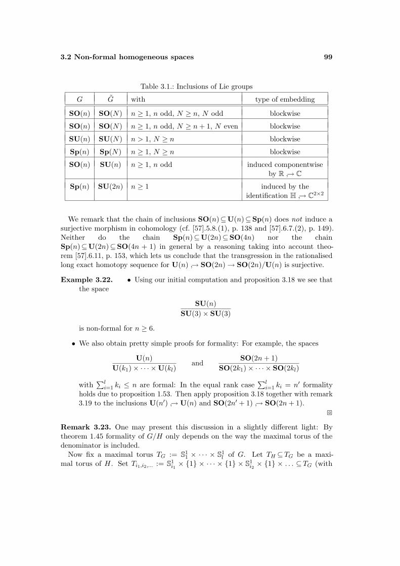
3.2 Non-formal homogeneous spaces 99
Table 3.1.: Inclusions of Lie groups
G G with type of embedding
SO(n) SO(N) n ≥ 1, n odd, N ≥ n, N odd blockwise
SO(n) SO(N) n ≥ 1, n odd, N ≥ n+ 1, N even blockwise
SU(n) SU(N) n > 1, N ≥ n blockwise
Sp(n) Sp(N) n ≥ 1, N ≥ n blockwise
SO(n) SU(n) n ≥ 1, n odd induced componentwiseby R → C
Sp(n) SU(2n) n ≥ 1 induced by theidentification H → C2×2
We remark that the chain of inclusions SO(n)⊆U(n)⊆Sp(n) does not induce asurjective morphism in cohomology (cf. [57].5.8.(1), p. 138 and [57].6.7.(2), p. 149).Neither do the chain Sp(n)⊆U(2n)⊆SO(4n) nor the chainSp(n)⊆U(2n)⊆SO(4n + 1) in general by a reasoning taking into account theo-rem [57].6.11, p. 153, which lets us conclude that the transgression in the rationalisedlong exact homotopy sequence for U(n) → SO(2n)→ SO(2n)/U(n) is surjective.
Example 3.22. • Using our initial computation and proposition 3.18 we see thatthe space
SU(n)SU(3)× SU(3)
is non-formal for n ≥ 6.
• We also obtain pretty simple proofs for formality: For example, the spaces
U(n)U(k1)× · · · ×U(kl)
andSO(2n+ 1)
SO(2k1)× · · · × SO(2kl)
with∑l
i=1 ki ≤ n are formal: In the equal rank case∑l
i=1 ki = n′ formalityholds due to proposition 1.53. Then apply proposition 3.18 together with remark3.19 to the inclusions U(n′) → U(n) and SO(2n′ + 1) → SO(2n+ 1).
Remark 3.23. One may present this discussion in a slightly different light: Bytheorem 1.45 formality of G/H only depends on the way the maximal torus of thedenominator is included.
Now fix a maximal torus TG := S11 × · · · × S1
l of G. Let TH ⊆TG be a maxi-mal torus of H. Set Ti1,i2,... := S1
i1× 1 × · · · × 1 × S1
i2× 1 × . . . ⊆TG (with
100 3 Rational Homotopy Theory
i1 < i2 < · · · ≤ l) to be the subtorus of TG containing only certain S1-components. Letfurther T ′ with TH ⊆T ′⊆TG be the smallest subtorus of TG of this form containingthe maximal torus of H, i.e.
T ′ :=⋂Ti1,i2,... | i1 < i2 < · · · ≤ l and TH ⊆Ti1,i2,...
Let WT ′ be the maximal subgroup of the Weyl group W(G) leaving T ′ invariant. Theclassical Lie groups of types An, Bn and Cn now have the following property: Themorphism
H∗(BG) = H∗(BTG)W(G) −→ H∗(BT ′)WT ′
induced by the inclusion is surjective. The algebra H∗(BG) is just the minimal modelof BG. The algebra H∗(BT ′)WT ′ is just the cohomology algebra of the subgroupG⊆G that corresponds to the block-matrices for which T ′ is the standard maximaltorus. In particular, we have that rk G = rkT ′. Thus the algebra H∗(BT ′)WT ′ mayalso be identified with the minimal model of BG. Thus also the map on minimalmodels induced by the inclusion G → G is surjective and the model of G lies in theone for G.
So in these cases the question whether G/H is formal or not just depends on(T ′,WT ′ , TH), the way TH includes into T ′ and the way WT ′ acts upon T ′; or in otherwords on (G, TH , φ : TH → G) only.
Let us now present one more result which serves to derive non-formality from somerather easily computable topological structures. This will simplify proofs for some ofthe known non-formal examples whilst producing a whole variety of further ones. Westart with a more general lemma.
Lemma 3.24. Let E2n+1 be a simply-connected compact manifold and let B2n be asimply-connected compact Kahler manifold (for n ≥ 1). Suppose there is a fibrationS1 → E
p−→ B. Assume further the following to hold true:
• The Euler class of p is a non-vanishing multiple of the Kahler class l of B inrational cohomology.
• The rational cohomology of B is concentrated in even degrees only.
• The rational homotopy groups of B are concentrated in degrees smaller or equalto n.
Then E is a non-formal space.
Proof. Since the Kahler class and the Euler class rationally are non-trivial multiples,we may formulate the Gysin sequence with rational coefficients for p as follows:
· · · → Hp(B) ∪l−→ Hp+2(B)→ Hp+2(E)→ Hp+1(B) ∪l−→ . . .
3.2 Non-formal homogeneous spaces 101
(The fibration is oriented, since B is simply-connected.) The Hard-Lefschetz propertyof B implies that taking the cup-product with l is injective in degrees p < n. So thesequence splits, yielding
Hp+2(B) = Hp(B)⊕Hp+2(E)
for −2 ≤ p ≤ n − 2. Since we assumed the odd-dimensional rational cohomologygroups of B to vanish we obtain in particular that
Hp(E) = 0 for odd p ≤ n(3.24)
Let(∧
VE ,dE)
be a minimal model of E. As E was supposed to be simply-connectedwe clearly have πp(E)⊗Q ∼= V p
E up to duality. By the long exact sequence of homotopygroups we obtain
πp(E) ∼= πp(B) for p ≥ 3
As we assumed
πp(B)⊗Q = 0 for p > n
we thus see that V >nE = 0 if n ≥ 2. If n = 1, we clearly still have V ≥3
E =0. So forarbitrary n ≥ 1 we obtain
V pE = 0 for odd p > n(3.25)
Assume now that E is formal. We shall lead this to a contradiction. By theorem1.41 we may split VE = CE ⊕NE with CE = ker dE |VE
and with the property thatevery closed element in I(NE) is exact.
By observation (3.24) we know that every closed element of odd degree in(∧
VE)≤n
is exact. Thus by the minimality of the model we directly derive that
(CE)≤n =(C≤nE
)even(3.26)
Together with (3.25) this implies that
CE = CevenE(3.27)
is concentrated in even degrees only. Hence so is∧CE . Thus, using the splitting∧
VE =∧CE ⊕ I(NE)
102 3 Rational Homotopy Theory
we derive from (3.27) and the formality of E that
Hodd(E) =(
ker dE |I(N)
im dE
)odd
= 0(3.28)
However, the manifold E is an odd-dimensional simply-connected compact manifold.Thus it satisfies Poincare Duality. It is orientable and possesses a volume form whichhence generates H2n+1(E) ∼= Q 6= 0. This contradicts formula (3.28). Thus E isnon-formal.
Remark 3.25. • We see that the proof works equally well if the spaces E and Bare not simply-connected but (have a finite fundamental group and) are simple,i.e. the action of the fundamental group on all homotopy groups (in positivedegree) is trivial. Indeed, the spaces then are orientable and the Gysin sequencecan be applied. Moreover, Rational Homotopy Theory is applicable to simplespaces without any change.
From proposition [64].1.17, p. 84, we see that the homogeneous space G/H of acompact connected Lie group G with connected closed Lie subgroup H is simple.
• From the proof of the lemma it is clear that we actually do not need to requireB to be Kahlerian. It is absolutely sufficient for B to have the Hard-Lefschetzproperty with respect to the Euler class. For example, this extends the lemmato the case of certain Donaldson submanifolds (cf. [23]) or biquotients (cf. [42]).
We may relax the prerequisites of the lemma even further: We need not require therational homotopy groups of B to be concentrated in degrees smaller or equal ton as long as the ones concentrated in odd degrees above n correspond to relationsin the minimal model of E via the long exact homotopy sequence; i.e. theyare not in the image of the dual of the rationalised Hurewicz homomorphism(cf. 1.27). Then the proof does not undergo any severe adaptation: We justobtain CpE = 0 instead of V p
E = 0 for odd p > n. This extends the lemma to thecase of non-elliptic spaces E and B.
• In theory, this lemma is not restricted to S1-fibrations. So for example usingthe Kraines form in degree four instead of the Kahler form in degree 2 one mayformulate a version for Positive Quaternion Kahler Manifolds. The formality ofthe 3-Sasakian manifolds associated to Wolf spaces, however, shows that suchan attempt seems to be less fruitful due to the other prerequisites in the lemma.
See the corollary on [64].13, p. 221 and the examples below for a related result inthe category of homogenous spaces. Let us now formulate the theorem that serves asthe main motivation for the preceeding lemma.
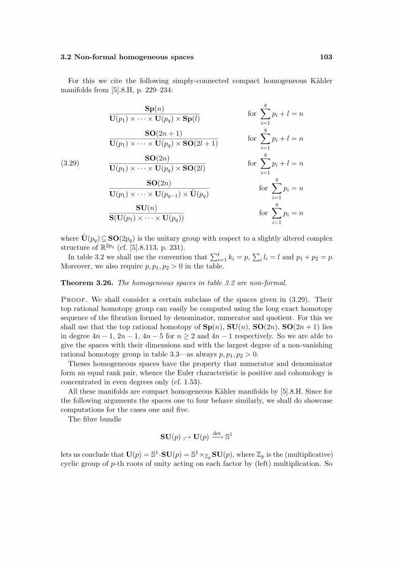
3.2 Non-formal homogeneous spaces 103
For this we cite the following simply-connected compact homogeneous Kahlermanifolds from [5].8.H, p. 229–234:
Sp(n)U(p1)× · · · ×U(pq)× Sp(l)
forq∑i=1
pi + l = n
SO(2n+ 1)U(p1)× · · · ×U(pq)× SO(2l + 1)
forq∑i=1
pi + l = n
SO(2n)U(p1)× · · · ×U(pq)× SO(2l)
forq∑i=1
pi + l = n(3.29)
SO(2n)U(p1)× · · · ×U(pq−1)× U(pq)
forq∑i=1
pi = n
SU(n)S(U(p1)× · · · ×U(pq))
forq∑i=1
pi = n
where U(pq)⊆SO(2pq) is the unitary group with respect to a slightly altered complexstructure of R2pq (cf. [5].8.113, p. 231).
In table 3.2 we shall use the convention that∑t
i=1 ki = p,∑
i li = l and p1 + p2 = p.Moreover, we also require p, p1, p2 > 0 in the table.
Theorem 3.26. The homogeneous spaces in table 3.2 are non-formal.
Proof. We shall consider a certain subclass of the spaces given in (3.29). Theirtop rational homotopy group can easily be computed using the long exact homotopysequence of the fibration formed by denominator, numerator and quotient. For this weshall use that the top rational homotopy of Sp(n), SU(n), SO(2n), SO(2n+ 1) liesin degree 4n− 1, 2n− 1, 4n− 5 for n ≥ 2 and 4n− 1 respectively. So we are able togive the spaces with their dimensions and with the largest degree of a non-vanishingrational homotopy group in table 3.3—as always p, p1, p2 > 0.
Theses homogeneous spaces have the property that numerator and denominatorform an equal rank pair, whence the Euler characteristic is positive and cohomology isconcentrated in even degrees only (cf. 1.53).
All these manifolds are compact homogeneous Kahler manifolds by [5].8.H. Since forthe following arguments the spaces one to four behave similarly, we shall do showcasecomputations for the cases one and five.
The fibre bundle
SU(p) → U(p) det−−→ S1
lets us conclude that U(p) = S1 ·SU(p) = S1×Zp SU(p), where Zp is the (multiplicative)cyclic group of p-th roots of unity acting on each factor by (left) multiplication. So
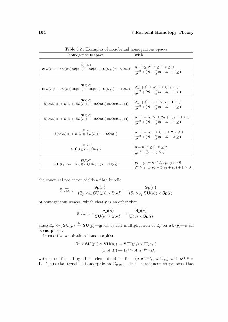
104 3 Rational Homotopy Theory
Table 3.2.: Examples of non-formal homogeneous spaceshomogeneous space with
Sp(N)S(U(k1)×···×U(kt))×Sp(l1)×···×Sp(lr)×U(lr+1)×···×U(ls) p+ l ≤ N , r ≥ 0, s ≥ 0
12p
2 + (2l − 72 )p− 4l + 1 ≥ 0
SU(N)S(U(k1)×···×U(kt))×Sp(l1)×···×Sp(lr)×U(lr+1)×···×U(ls) 2(p+ l) ≤ N , r ≥ 0, s ≥ 0
12p
2 + (2l − 72 )p− 4l + 1 ≥ 0
SO(N)S(U(k1)×···×U(kt))×SO(2l1)×···×SO(2lr)×SO(2lr+1+1) 2(p+ l) + 1 ≤ N , r + 1 ≥ 0
12p
2 + (2l − 72 )p− 4l + 1 ≥ 0
SU(N)S(U(k1)×···×U(kt))×SO(2l1)×···×SO(2lr)×SO(2lr+1+1) p+ l = n, N ≥ 2n+ 1, r + 1 ≥ 0
12p
2 + (2l − 72 )p− 4l + 1 ≥ 0
SO(2n)S(U(k1)×···×U(kt))×SO(2l1)×···×SO(2lr) p+ l = n, r ≥ 0, n ≥ 2, l 6= 1
12p
2 + (2l − 92 )p− 4l + 5 ≥ 0
SO(2n)
S(U(k1)×···×U(kt))p = n, r ≥ 0, n ≥ 212n
2 − 92n+ 5 ≥ 0
SU(N)S(U(k1)×···×U(ks))×S(U(ks+1)×···×U(kt))
p1 + p2 = n ≤ N , p1, p2 > 0N ≥ 2, p1p2 − 2(p1 + p2) + 1 ≥ 0
the canonical projection yields a fibre bundle
S1/Zp →Sp(n)
(Zp ×Zp SU(p))× Sp(l)→ Sp(n)
(S1 ×Zp SU(p))× Sp(l)
of homogeneous spaces, which clearly is no other than
S1/Zp →Sp(n)
SU(p)× Sp(l)→ Sp(n)
U(p)× Sp(l)
since Zp ×Zp SU(p)∼=−→ SU(p)—given by left multiplication of Zp on SU(p)—is an
isomorphism.In case five we obtain a homomorphism
S1 × SU(p1)× SU(p2)→ S(U(p1)×U(p2))(x,A,B) 7→ (xp2 ·A, x−p1 ·B)
with kernel formed by all the elements of the form (a, a−p2Ip1 , ap1Ip2) with ap1p2 =
1. Thus the kernel is isomorphic to Zp1p2 . (It is consequent to propose that
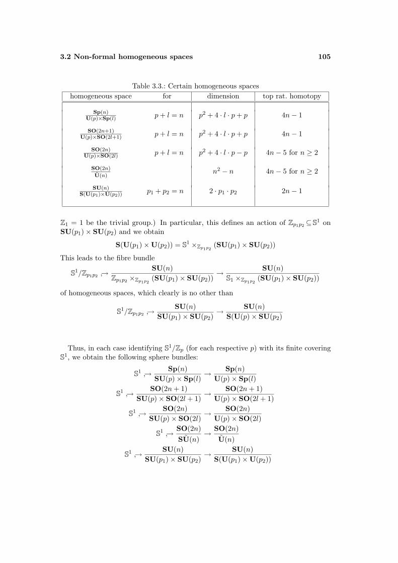
3.2 Non-formal homogeneous spaces 105
Table 3.3.: Certain homogeneous spaceshomogeneous space for dimension top rat. homotopy
Sp(n)U(p)×Sp(l) p+ l = n p2 + 4 · l · p+ p 4n− 1
SO(2n+1)U(p)×SO(2l+1) p+ l = n p2 + 4 · l · p+ p 4n− 1
SO(2n)U(p)×SO(2l) p+ l = n p2 + 4 · l · p− p 4n− 5 for n ≥ 2
SO(2n)
U(n)n2 − n 4n− 5 for n ≥ 2
SU(n)S(U(p1)×U(p2)) p1 + p2 = n 2 · p1 · p2 2n− 1
Z1 = 1 be the trivial group.) In particular, this defines an action of Zp1p2 ⊆S1 onSU(p1)× SU(p2) and we obtain
S(U(p1)×U(p2)) = S1 ×Zp1p2(SU(p1)× SU(p2))
This leads to the fibre bundle
S1/Zp1p2 →SU(n)
Zp1p2 ×Zp1p2(SU(p1)× SU(p2))
→ SU(n)S1 ×Zp1p2
(SU(p1)× SU(p2))
of homogeneous spaces, which clearly is no other than
S1/Zp1p2 →SU(n)
SU(p1)× SU(p2)→ SU(n)
S(U(p)× SU(p2)
Thus, in each case identifying S1/Zp (for each respective p) with its finite coveringS1, we obtain the following sphere bundles:
S1 → Sp(n)SU(p)× Sp(l)
→ Sp(n)U(p)× Sp(l)
S1 → SO(2n+ 1)SU(p)× SO(2l + 1)
→ SO(2n+ 1)U(p)× SO(2l + 1)
S1 → SO(2n)SU(p)× SO(2l)
→ SO(2n)U(p)× SO(2l)
S1 → SO(2n)SU(n)
→ SO(2n)U(n)
S1 → SU(n)SU(p1)× SU(p2)
→ SU(n)S(U(p1)×U(p2))
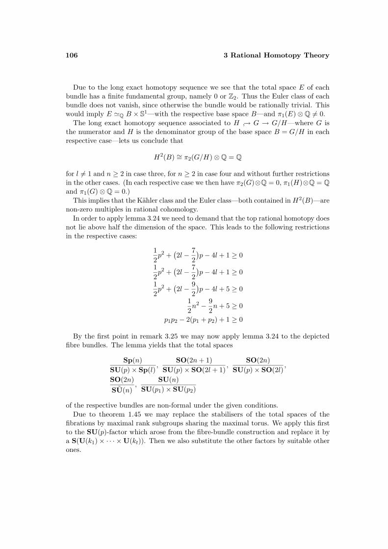
106 3 Rational Homotopy Theory
Due to the long exact homotopy sequence we see that the total space E of eachbundle has a finite fundamental group, namely 0 or Z2. Thus the Euler class of eachbundle does not vanish, since otherwise the bundle would be rationally trivial. Thiswould imply E 'Q B × S1—with the respective base space B—and π1(E)⊗Q 6= 0.
The long exact homotopy sequence associated to H → G → G/H—where G isthe numerator and H is the denominator group of the base space B = G/H in eachrespective case—lets us conclude that
H2(B) ∼= π2(G/H)⊗Q = Q
for l 6= 1 and n ≥ 2 in case three, for n ≥ 2 in case four and without further restrictionsin the other cases. (In each respective case we then have π2(G)⊗Q = 0, π1(H)⊗Q = Qand π1(G)⊗Q = 0.)
This implies that the Kahler class and the Euler class—both contained in H2(B)—arenon-zero multiples in rational cohomology.
In order to apply lemma 3.24 we need to demand that the top rational homotopy doesnot lie above half the dimension of the space. This leads to the following restrictionsin the respective cases:
12p2 +
(2l − 7
2)p− 4l + 1 ≥ 0
12p2 +
(2l − 7
2)p− 4l + 1 ≥ 0
12p2 +
(2l − 9
2)p− 4l + 5 ≥ 0
12n2 − 9
2n+ 5 ≥ 0
p1p2 − 2(p1 + p2) + 1 ≥ 0
By the first point in remark 3.25 we may now apply lemma 3.24 to the depictedfibre bundles. The lemma yields that the total spaces
Sp(n)SU(p)× Sp(l)
,SO(2n+ 1)
SU(p)× SO(2l + 1),
SO(2n)SU(p)× SO(2l)
,
SO(2n)SU(n)
,SU(n)
SU(p1)× SU(p2)
of the respective bundles are non-formal under the given conditions.Due to theorem 1.45 we may replace the stabilisers of the total spaces of the
fibrations by maximal rank subgroups sharing the maximal torus. We apply this firstto the SU(p)-factor which arose from the fibre-bundle construction and replace it bya S(U(k1)× · · · ×U(kt)). Then we also substitute the other factors by suitable otherones.
3.2 Non-formal homogeneous spaces 107
Finally, we are done by an application of proposition 3.18 respectively table 3.1,which allows us to use the described embeddings of the numerator into larger Liegroups to form new homogeneous spaces. The result of this process is depicted intable 3.2:
The first example we considered here leads to the first line in 3.2 by blockwiseinclusion Sp(n) → Sp(N) and to the second line by the inclusion
Sp(n) → SU(2n) → SU(N)
(which is identical to Sp(n) → Sp(N ′) → SU(2N ′) → SU(N)).The second example produces lines three and four by the inclusions
SO(2n+ 1) → SO(N) and
SO(2n+ 1) → SU(2n+ 1) → SU(N)
(which is the same as SO(2n+ 1) → SO(N ′) → SU(2N ′) → SU(N)).For examples three and four we do not use any further inclusions. Example five
produces line seven by the inclusion SU(n) → SU(N).
The proof guides the way of how to interpret table 3.2. Nonetheless, let us—exemplarily for the first line of the table—shed some more light upon the usedinclusions: The inclusion of the denominator in the first example is given by blockwiseinclusions of
S(U(k1)× · · · ×U(kt)) → Sp(p) → Sp(n) → Sp(N)
Sp(l1)× · · · × . . .Sp(lr) → Sp( r∑i=1
li
)→ Sp(n) → Sp(N)
U(lr+1)× · · · × . . .U(ls) → Sp( s∑i=r+1
li
)→ Sp(n) → Sp(N)
where n = p+∑s
i=1 li.In examples three and four it does not matter whether or not we have a stabiliser
which has—beside the unitary part—special orthogonal groups of the type SO(2li)only, if there is additionally one factor of the form SO(2lr+1 +1) or if there is the factorSO(2lr + 1) only: All three cases establish maximal rank subgroups of SO(2l + 1),which therefore share the maximal torus with SO(2l + 1).
Moreover, note that the relations in table 3.2 are growing quadratically in p. Thusfor a constant l we can always find p and N that will satisfy the restrictions.
Example 3.27. Let us describe some of the simplest and most classical consequencesthat arise out of our reasoning. We have proved that the spaces
Sp(n)SU(n)
SO(2n)SU(n)
SU(p+ q)SU(p)× SU(q)
108 3 Rational Homotopy Theory
are non-formal for n ≥ 7, n ≥ 8 and p+ q ≥ 4 respectively.
We observe that the homogeneous 3-Sasakian manifolds—fibring over the twistorspace of a Positive Quaternion Kahler Manifold—do not satisfy the assumption on thedimension in lemma 3.24—although they are quite close to it. Their formality showsthat the prerequisites in the lemma cannot be relaxed too much. In the same directiongoes the following proposition: The prerequisites in the last example in table 3.2 forthe space to be non-formal are evidently satisfied if p1, p2 ≥ 4 or if p ≥ 3 and p ≥ 5.These are sharp bounds:
Proposition 3.28. The homogeneous space
SU(7)SU(3)× SU(4)
is formal.
Proof. Using the model (3.21) we compute a minimal model for the given homoge-neous space as generated by
c, c′, x deg c = 4, deg c′ = 6, deg x = 13
and by relations
x1, x2 deg x1 = 9, deg x2 = 11
with
d(x1) = c · c′, d(x2) = c3 + (c′)2
This model is formal.
As for the interlink between formality and geometry we remark that, for example,from the computations in lemma [4].8.2, p. 272, we directly see that all known odd-dimensional examples—cf. proposition[4].8.1, p. 271—of positively curved Riemannianmanifolds are formal spaces.
The importance of formality issues in geometry is also stressed by the following resultin [4]. Non-formality of C := SU(6)
SU(3)×SU(3) plays a crucial role for the construction of acounterexample (cf. [4], theorem 1.4): It gives rise to the existence of a non-negativelycurved vector bundle over C × T (with a torus T of dimT ≥ 2) which does not splitin a certain sense as a product of bundles over the factors of the base space, butwhich has the property that its total space admits a complete metric of non-negativesectional curvature with the zero section is a soul.
3.2 Non-formal homogeneous spaces 109
Moreover, we remark that we have found simply-connected examples of homogeneousspaces M1 and M2 with the property that χ(M2) > 0—i.e. M2 is formal in particular(cf. 1.52)—and that M1 is not formal whilst they fibre as
S1 →M1 →M2
However, it is not possible to find manifolds M1 and M2 as described that fibre in theform
M2 →M1 → S1
This is due to the fact that the Halperin conjecture (cf. p. 71) has been confirmed onhomogeneous spaces (cf. [69], theorem A, p. 81) and theorem [56].3.4, p. 12.
It was established that simply-connected compact manifolds of dimension at most sixare formal spaces. In [24] Fernandez and Munoz pose the question whether there arenon-formal simply-connected compact manifolds in dimensions seven and higher. Theyanswer this in the affirmative by constructing seven-dimensional and eight-dimensionalexamples. The requested example in a certain dimension above dimension seven isthen obviously given by a direct product with the corresponding even-dimensionalsphere. This leads to the problem of constructing highly-connected examples (cf. forexample [26]). Note that the methods of constructing these manifolds involve surgerytheory, in particular.
We shall use a slightly different approach towards this issue by using homogeneousspaces.
Proposition 3.29. In every dimension d ≥ 72 there is an irreducible simply connectedcompact homogeneous space which is not formal. In particular, every such spaceconstitutes a rationally elliptic non-formal example.
Proof. The example
SU(N)S(U(k1)× · · · ×U(ks))× S(U(ks+1)× · · · ×U(kt))
from table 3.2 will serve us as a main source of further examples. (It is simply-connectedas so is the numerator group.)
The restrictions in the table will certainly be satisfied if p1, p2 ≥ 4 or if p1 ≥ 3 andp2 ≥ 5 (respectively N ≥ p1 + p2). By our initial computations we may also use thecase for p1 = p2 = 3. We use a slightly different terminology: Set p := p1, k := p2 and
110 3 Rational Homotopy Theory
N ≥ 0. Thus whenever p = k = 3 or p, k ≥ 4 or p ≥ 3 and k ≥ 5 the spaces
SU(p+ k +N)SU(p)× SU(k)
(3.30)
SU(p+ k +N)SU(p)× S(U(k − 1)×U(1))
(3.31)
SU(p+ k +N)S(U(p− 1)×U(1))× SU(k)
(3.32)
SU(p+ k +N)S(U(p− 1)×U(1))× S(U(k − 1)×U(1))
(3.33)
SU(p+ k +N)S(U(p− 2)×U(2))× SU(k)
(3.34)
SU(p+ k +N)S(U(p− 2)×U(2))× S(U(k − 1)×U(1))
(3.35)
SU(p+ k +N)S(U(p− 2)×U(2))× S(U(k − 2)×U(1)×U(1))
(3.36)
SU(p+ k +N)S(U(p− 2)×U(1)×U(1))× SU(k)
(3.37)
SU(p+ k +N)S(U(p− 2)×U(1)×U(1))× S(U(k − 2)×U(2))
(3.38)
SU(p+ k +N)S(U(p− 2)×U(1)×U(1))× S(U(k − 2)×U(1)×U(1))
(3.39)
will be non-formal. In the given order the spaces have the following dimensions:
2(k +N)p+ (2kN +N2 + 1)
2(k +N)p+ (2kN +N2 + 2k − 1)
2(k +N + 2)p+ (2kN +N2 − 1)
2(k +N + 2)p+ (2kN +N2 + 2k − 3)
2(k +N + 4)p+ (2kN +N2 − 7)(3.40)
2(k +N + 4p+ (2kN +N2 + 2k − 9)
2(k +N + 4)p+ (2kN +N2 + 4k − 13)
2(k +N + 4)p+ (2kN +N2 − 5)
2(k +N + 4)p+ (2kN +N2 + 4k − 13)
2(k +N + 4)p+ (2kN +N2 + 4k − 11)
Regard the manifolds as parametrised over N by the variable p. So we have the infinitesequences (Mk,N
p )(3.30)p∈N , . . . , (Mk,N
p )(3.39)p∈N . We shall now show that for each congruence
class [m] modulo 16 there is a family (Mk,Np )mp∈N which—for certain numbers p—consists
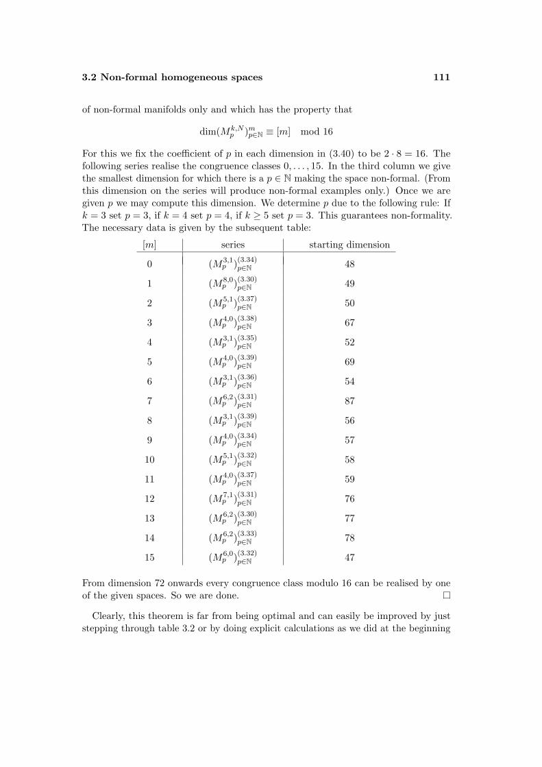
3.2 Non-formal homogeneous spaces 111
of non-formal manifolds only and which has the property that
dim(Mk,Np )mp∈N ≡ [m] mod 16
For this we fix the coefficient of p in each dimension in (3.40) to be 2 · 8 = 16. Thefollowing series realise the congruence classes 0, . . . , 15. In the third column we givethe smallest dimension for which there is a p ∈ N making the space non-formal. (Fromthis dimension on the series will produce non-formal examples only.) Once we aregiven p we may compute this dimension. We determine p due to the following rule: Ifk = 3 set p = 3, if k = 4 set p = 4, if k ≥ 5 set p = 3. This guarantees non-formality.The necessary data is given by the subsequent table:
[m] series starting dimension
0 (M3,1p )(3.34)
p∈N 48
1 (M8,0p )(3.30)
p∈N 49
2 (M5,1p )(3.37)
p∈N 50
3 (M4,0p )(3.38)
p∈N 67
4 (M3,1p )(3.35)
p∈N 52
5 (M4,0p )(3.39)
p∈N 69
6 (M3,1p )(3.36)
p∈N 54
7 (M6,2p )(3.31)
p∈N 87
8 (M3,1p )(3.39)
p∈N 56
9 (M4,0p )(3.34)
p∈N 57
10 (M5,1p )(3.32)
p∈N 58
11 (M4,0p )(3.37)
p∈N 59
12 (M7,1p )(3.31)
p∈N 76
13 (M6,2p )(3.30)
p∈N 77
14 (M6,2p )(3.33)
p∈N 78
15 (M6,0p )(3.32)
p∈N 47
From dimension 72 onwards every congruence class modulo 16 can be realised by oneof the given spaces. So we are done.
Clearly, this theorem is far from being optimal and can easily be improved by juststepping through table 3.2 or by doing explicit calculations as we did at the beginning
112 3 Rational Homotopy Theory
of the section. Indeed, in the proof we have found non-formal homogeneous spaces indimensions
47, 48, 49, 50, 52, 54, 56, 57, 58, 59, 63, 64, 65, 66, 67, 68, 69, 70
and from dimension 72 onwards.We remark that one clearly may use other non-formal series like Sp(n)/SU(n) in
order to establish similar results. Since the number of partitions of a natural numbern ∈ N is growing exponentially in n one will find many stabilisers sharing their maximaltori with SU(n).
As we pointed out, compact homogeneous spaces are rationally elliptic. Thus thequestion that arises naturally is: In which dimensions are there examples of non-formalelliptic simply-connected irreducible compact manifolds?
We end this section by partly generalising theorem 1.45 which asserts that theformality of a homogeneous space G/H of a connected compact Lie group G anda connected subgroup H is equivalent to the formality of G/T , where T ⊆H is amaximal torus of H. We shall show that one direction can easily be seen to hold trueon a biquotient as well.
For this recall that whenever H acts freely on a topological space X we obtain thefibre bundle:
H/T → X/Tp−→ X/H(3.41)
where p is the canonical projection [x] 7→ [[x]]. Indeed, the fibre F[[x]] at a point [[x]] is
F[[x]] = [y] ∈ X/T | p([y]) = [[x]]=
[y] ∈ X/T | ∃h[y] ∈ H : h[y] · [y] = [x]
where H acts on X/T by h · [x] = [h · x]. The assignment
F[[x]] → H/T
[y] 7→ h[y]T
is well-defined and a homeomorphism.
Proposition 3.30. Let G be a connected compact Lie group and let H be a connectedclosed subgroup of G×G with maximal torus T ⊆H of H. Suppose one of GH andGT to be simply-connected.
Then we obtain: If the biquotient GH is formal, so is GT .
Proof. Due to (3.41) we form the fibre bundle
H/T → GT → GH
3.3 Pure models and Lefschetz-like properties 113
of simply-connected spaces. Indeed, by proposition [64].1.19, p. 84, the homogeneousspace H/T is simply-connected, as rkT = rkH. The long exact homotopy sequencethen yields π1(GT ) ∼= π1(GH). One of these two groups vanishes by assumptionand so do both of them.
The homogeneous space H/T satisfies the Halperin conjecture (cf. [69], theoremA, p. 81). Thus every fibration of simply-connected spaces with fibre H/T is totallynon-cohomologous to zero. Theorem [56].3.4, p. 12, then yields the result.
3.3. Pure models and Lefschetz-like properties
The last section was dedicated to the interplay of homogeneity and formality. In thissection we shall generalise the setting to pure Sullivan models. Recall that a Sullivanalgebra
(∧V,d
)is called pure if V is finite-dimensional and if
∧V =
∧V even⊗
∧V odd
with d|V even = 0 and d(V odd)⊆∧V even—cf. definition 1.51.
Hence, in geometric terms, we no longer focus on homogeneous spaces, since forexample also biquotients enter the stage (cf. 1.53).
A second special feature which we shall take into consideration will be a Lefschetz-likeproperty.
The classical Hard-Lefschetz property for Kahler manifolds M2n states that
∪[ω]n−k : Hk(M)∼=−→ H2n−k(M)(3.42)
is an isomorphism for all 0 ≤ k ≤ n. The form ω is the Kahler form of degree two.On Positive Quaternion Kahler Manifolds M4n we have an analogue with the Krainesform ω of degree four (cf. 1.13):
∪[ω]n−k : H2k(M)∼=−→ H4n−2k(M)(3.43)
(which is as powerful as the corresponding property for Kahler manifolds, since odddegree rational cohomology is known to vanish—cf. 1.13.) In each case a directconsequence of the Hard-Lefschetz property is that the volume form v is a multiple of[ω]n. In terms of a minimal Sullivan model
(∧V,d
)of M this will imply—at least
in the simply-connected case—that v may be regarded as lying in∧V even, which, in
general, is a weaker statement.Similar but weaker properties than the Hard-Lefschetz properties can be found on
Riemannian manifolds with special holonomy—such as Joyce manifolds.Thus we shall consider special topological properties that have effects in very concrete
geometric situations. Consequently, as one possible “dictionary” we suggest
114 3 Rational Homotopy Theory
geometry ! algebra
compact biquotient !pure Sullivan model (with non-degenerate cup
product pairing)
(non-symmetric) specialholonomy
! (Hard-)Lefschetz-like property
So let us begin with an investigation on formality of spaces with pure models by meansof the restrictions imposed by a (Hard-)Lefschetz-like property.
In [42] and [4] the question arises when a biquotient is a Kahler manifold. Theanswer to that is unknown even for simplest examples as S1\U(3)/T 2—which satisfiesHard-Lefschetz. The main motivation for this is that by a result of Meier’s (cf. [58],[59]) Hard-Lefschetz spaces—and compact Kahler manifolds, in particular—satisfythe Halperin conjecture (cf. p. 71). Moreover, it is not clear at all whether justsimple examples like S1\Sp(n)/SU(n) have the Hard-Lefschetz property. So the latterdeserves some more attention.
We commence our considerations with the following lemma (which is said to holdon homogeneous spaces in [4], p. 280).
Proposition 3.31. A pure minimal Sullivan algebra (∧V,d) is formal if and only if
it is of the form (∧V,d
) ∼= (∧V ′,d)⊗(∧〈z1, . . . , zl〉, 0
)(3.44)
(for maximal such l) with a pure minimal Sullivan algebra (∧V ′, d) of positive Euler
characteristic—which is automatically formal then—and with odd degree generators zi.
Proof. Choose a basis z1, . . . , zm of V odd with the property that dzi = 0 for1 ≤ i ≤ l—and some fixed 1 ≤ l ≤ m—and that d|〈zl+1,...,zm〉 is injective. Frompureness it follows:
d(〈z1, . . . , zl〉) = 0
d(〈zl+1, . . . , zm〉) ∈∧V even
d(V even) = 0
Thus we obtain(∧V,d
)=(∧
(V even ⊕ 〈zl+1, . . . , zm〉), d)⊗(∧〈z1, . . . , zl〉, 0
)Set V ′ := V even ⊕ 〈zl+1, . . . , zm〉. The minimality of
(∧V,d
)enforces the minimality
of(∧
V ′, d)
and(∧
V ′,d)
is again a pure minimal Sullivan algebra. (It is a Sullivanalgebra as the filtration of V that made
(∧V,d
)a Sullivan algebra restricts to
3.3 Pure models and Lefschetz-like properties 115
a filtration on V ′—cf. the definition on [22].12, p. 138—since both(∧
V ′, d)
and(∧〈zl+1, . . . , zm〉, 0
)are differential subalgebras.)
By theorem 1.47 the formality of(∧
V,d)
now is equivalent to the formality of(∧V ′, d).If(∧
V ′, d)
has positive Euler characteristic, it is formal by theorem 1.52, since itis positively elliptic. Thus
(∧V,d
)then is formal, too.
For the reverse implication we use contraposition: Suppose the Euler characteristicof(∧
V ′, d)
to vanish. We shall show that the algebra is non-formal. The algebra(V ′, d
)has the property that d((V ′)even) = 0 and that d|(V ′)odd is injective. Thus,
setting C := (V ′)even and N := (V ′)odd, yields a decomposition V ′ = C⊕N as requiredin theorem 1.41 and this decomposition is uniquely determined.
Due to χ(∧
V ′,d)
= 0 there is a closed and non-exact element x in(∧
V ′,d)
thathas odd degree. Therefore x necessarily lies in I(N). Thus
(∧V ′, d
)is not formal
and neither is(∧
V,d).
By abuse of notation we shall speak of volume forms as top cohomology generatorsof simply-connected elliptic Sullivan algebras. Volume forms then need to be uniqueup to multiples by [21], theorem A, p. 70. So we shall refer to it as to “the” volumeform.
Proposition 3.32. Let(∧
V,d)
be a simply-connected pure minimal Sullivan algebrawith the property that its volume form [v] ∈ H
(∧V,d
)is represented by some closed
v ∈∧V even.
Then the following assertions hold: The algebra(∧
V,d)
is positively elliptic, i.e. itsrational cohomology is concentrated in even degrees only. In particular, it is formal.
Proof. We split the algebra as in (3.44). Thus a volume form of(∧
V,d)
necessarilyhas to be of the form v = v ·z1 ·· · ··zl 6= 0 with v a volume form of
(∧V ′,d
). Recall that
the zi ∈ V are of odd degree. So v ∈∧V even requires l = 0 and
(∧V,d
)=(∧
V ′,d).
Suppose the algebra(∧
V,d)
is non-formal. Thus there is a closed non-exact elementx 6= 0 in the ideal I(N) generated by N = V odd—cf. the proof of proposition 3.31—in∧V .Due to [21], theorem A, p. 70, simply-connected elliptic spaces have the homotopy
type of finite Poincare complexes. Thus by the non-singularity of the cup-productpairing we see that there is an element x′ ∈
(∧V,d
)such that x · x′ represents a
non-vanishing element in (rational) top cohomology. By our assumption and by theuniqueness of the volume form we now derive that
[x · x′ − kv] = 0 ∈ H(∧
V,d)
for some 0 6= k ∈ Q. Hence there is a form y ∈(∧
V,d)
with dy = x · x′ − kv.Now we use the fact that on a pure algebra we have the lower grading, i.e.:
d :∧V even ⊗
∧l V odd →
∧V even ⊗
∧l−1 V odd
116 3 Rational Homotopy Theory
Now we shall see that the form x · x′ lies in∧V even ⊗
∧>0 V odd whereasv ∈
∧V even ⊗
∧0 V odd by assumption. This is due to the fact that the elementx is in the ideal I(N) generated by N = V odd in
∧V , i.e. x ∈
∧V even ⊗
∧>0 V odd.So we also obtain
x · x′ ∈∧V even ⊗
∧>0V odd
By the lower grading we obtain a direct sum decomposition y =∑l
i=0 yl withyi ∈
∧V even ⊗
∧i V odd. Without restriction we may assume that y0 = 0. Hence wesee that y = y1 + · · ·+ yl, i.e. y = y1 + y with
y = y2 + · · ·+ yl ∈∧V even ⊗
∧>0 V odd
Thus
d(y1) ∈∧V even ⊗
∧0 V odd =
∧V even 3 kv
d(y) ∈∧V even ⊗
∧>0 V odd 3 x · x′
Since dy1 + dy = dy = −kv + x · x′, the lower grading directly implies that dy1 = −kvand that dy = x · x′. This, however, contradicts the fact that both [v] and [x · x′] werevolume forms and consequently it contradicts the choice of x. Thus there is no closednon-exact element x ∈ I(N).
Thus the algebra(∧
V,d)
=(∧
V ′,d)
is formal by 1.41. By proposition 3.31 thisis exactly the case if (
∧V,d) has positive Euler characteristic. This, however, is
equivalent to the vanishing of odd-degree homology and finishes the proof.
Recall that symplectic manifolds M2n, i.e. smooth manifolds with closed, non-degenerate 2-form ω, have the following property: The symplectic form ω ∈ A2
DR(M)is closed and satisfies ωn(p) 6= 0 for all p ∈M . This is equivalent to the non-degeneracyof ω. Compact Kahler manifolds are symplectic in particular.
A weaker version of symplecticity is the following: A manifold M2n is calledcohomologically symplectic if there is a class η ∈ H2(M2n) with ηn 6= 0. Clearly, Hard-Lefschetz manifolds—in the version of formula (3.42)—are cohomologically symplectic.
Theorem 3.33. Let M be a simply-connected manifold which admits a pure Sullivanmodel. Suppose that one of the following statements holds:
• The manifold M2n is cohomologically symplectic.
• The manifold M4n satisfies Hard-Lefschetz in the version of formula (3.43).
Then M is formal and has cohomology concentrated in even degrees only.
3.3 Pure models and Lefschetz-like properties 117
Proof. We form a pure minimal Sullivan model(∧
V,d)
for M . We shall show thatits non-degeneracy requires the volume form to be represented by an element in thesubalgebra generated by even-degree elements:
In the first case of the assertion we shall show that the cohomology-symplecticform [ω] ∈ H2(M) satisfies ω ∈
∧V even. We then derive that ωn is a volume form in∧
V even.So we have degω = 2 and we directly see that ω is not decomposable, since the
manifolds are simply-connected. This implies that ω ∈ V 2.
In the second case we consider the form ω in degree four with respect to which wehave Hard-Lefschetz. Clearly, ωn is a volume form. So we shall show that ω ∈
∧V even
which will yield the result.Every decomposition of ω would have to be done by linear combinations of products
of two elements (as there are none in degree one). These two elements may noweither be of degree two both or one of degree one and the other of degree three. Thelatter possibility again is excluded by simply-connectedness. So even if the form ω isdecomposable, it still remains in
∧V even.
By proposition 3.32 we may now derive the result on cohomology and formality.
Remark 3.34. • In the case of simply-connected (Positive Quaternion) KahlerManifolds with pure model we might have just proceeded as follows: Use theirformality to see that
(∧V ′, d
)in decomposition (3.44) is formal, whence it is
positively elliptic. Use “cohomologically symplectic” to realise that V ′ = V .
• Theorem 3.33—either applied to the twistor space or to the manifold itself—mayserve as a reproof of the vanishing of odd-degree Betti numbers and of formalityfor Positive Quaternion Kahler Manifolds within the class of simply-connectedmanifolds admitting pure models.
• Define a quaternionic cohomologically symplectic manifold in an analogous fashion.This property instead of the quaternionic Hard-Lefschetz property (3.43) clearlywould have been sufficient to conclude the theorem.
• From [60] and [13].5, p. 79–94, we deduce that a generalised ddc-lemma on acompact symplectic manifold holds if and only if the manifold satisfies Hard-Lefschetz. Nonetheless, the manifold then needs not be formal in general. In thelight of theorem 3.33 it is so, however, if the manifold admits a pure model.
• In example [14].4.4, p. 346, an example of a 12-dimensional non-formal simply-connected symplectic Hard-Lefschetz manifold is given.
• We remark that there are several examples of Hard-Lefschetz manifolds that arenot Kahlerian although they are formal. For example see [23], proposition 6.2,p. 171, where certain four-dimensional Donaldson submanifolds are shown tobe symplectic, to satisfy Hard-Lefschetz but to admit no complex structures;
118 3 Rational Homotopy Theory
i.e. there is no Kahler structure, in particular. See theorem [25].3.5, p. 3322,for examples of cohomologically Kahler manifolds that admit no Kahler metric.(They are formal and satisfy Hard-Lefschetz.)
We shall now derive topological properties of some particular manifolds with holon-omy G2 or Spin(7).
In proposition [41].10.2.6, p. 246, it is proved that a compact G2-manifold M7, i.e. amanifold M with Hol(M) = G2, satisfies
〈a ∪ a ∪ [ω], [M ]〉 < 0(3.45)
for every non-zero a ∈ H2(M) and with respect to the 3-form ω defining the G2-structure (cf. [41].10.1.1, p. 242). The analogue holds for compact Spin(7)-manifolds(cf. [41].6.6, p. 261) with the respective 4-form ω (cf. [41].10.5.1, p. 255). So, inparticular, combining this with Poincare Duality one obtains Lefschetz-like propertiesfor manifolds with holonomy G2 or Spin(7):
∪ω : H2(M)∼=−→ Hn−2(M)
for the closed 3-form ω defining the G2-structure and n = 7; respectively the 4-form ωdefining the Spin(7)-structure and n = 8.
If Hol(M) = Spin(7), theorem [41].10.6.8, p. 261, gives further strong topologicalrestrictions; there is the following relation on Betti numbers:
b3 + b+4 = b2 + 2b−4 + 25(3.46)
where b+4 + b−4 = b4 and b+4 ≥ 1. The manifold is simply-connected and spin withA(M)[M ] = 1—cf. [41], equation (10.25) on page 260, together with proposition 10.6.5,p. 260. A direct consequence of the latter result is that there are no smooth effectiveS1-actions upon M due to [3]—compare the refined version given by theorem 2.5.In particular, we shall not find any homogeneous space that admits a metric withsuch holonomy. Using the relation on Betti numbers this can be generalised withease. For this recall— we adapt the formulas (1.8), (1.9), (1.11) and (1.12) to ourcase—that for an elliptic orientable compact manifold—these properties imply thatthe formal/homological dimension equals dimM—the following equations hold:∑
i
deg xi ≤ 2 · dimM − 1(3.47) ∑i
deg yi ≤ dimM(3.48)
dimπ∗(M)⊗Q ≤ dimM(3.49) ∑i
deg xi −∑j
(deg yj − 1) = dimM(3.50)
3.3 Pure models and Lefschetz-like properties 119
Again, the xi form a homogeneous basis of πodd ⊗Q and the yi form a homogeneousbasis of πeven ⊗Q.
Using these relations we shall prove
Proposition 3.35. A rationally elliptic compact manifold does not admit a metric gwith Holg(M) = Spin(7).
Proof. Relation (3.46) yields b4 ≥ b+4 ≥ b2 − b3 + 25 and b3 + b4 ≥ b2 + 25. Let(∧V,d
)be the minimal model of M . Since M is simply-connected we obtain that
dimπ2(M)⊗Q = dimV 2 = b2
dimπ3(M)⊗Q = dimV 3 ≥ b3
dimπ4(M)⊗Q = dimV 4 ≥ b4 − dim Sym2(V 2) = b4 −b2(b2 + 1)
2
In particular, we see that
dimπ∗(M)⊗Q ≥ b2 + b3 +(b4 −
b2(b2 + 1)2
)= b3 + b4 +
b2(1− b2)2
≥ 25 + b2 +b2(1− b2)
2
= 25 +b2(3− b2)
2
Since we have that dimV 2 = b2 equation (3.48) yields in particular that2 · b2 ≤ dimM = 8 and that b2 ≤ 4. Thus we derive that dimπ∗(M) ⊗ Q ≥ 23,which contradicts (3.49).
A G2-manifold is known to have a finite fundamental group (cf. [41].10.2.2, p. 245).We shall now shed a light on the rational homotopy type of an elliptic simply-connectedG2-manifold.
Proposition 3.36. Let M be a simply-connected compact elliptic manifold that admitsa Riemannian metric g with Holg(M) = G2. Then a minimal model
(∧V,d
)of M
is one of the following models, which we describe by the graded vector space V . Wegive generators in their respective degree together with their differentials when possible.In the first two cases the model is completely described. In the third case we obtain afamily of models depending on the differentials of x and x′.
2 : a 7→ 0 3 : ω 7→ 0 2 : a 7→ 0, b 7→ 03 : ω 7→ 0 4 : a 7→ 0 3 : ω 7→ 0, x 7→?, x′ 7→?
5 : x 7→ a3 7 : x 7→ a2
120 3 Rational Homotopy Theory
The first case has the rational homotopy type of CP2 × S3 and the second one has therational homotopy type of S3 × S4. In the third case d|〈x,x′〉 is injective.
Moreover, in any case the minimal model is formal.
Proof. A G2-manifold is 7-dimensional. In particular, by Poincare Duality its Eulercharacteristic vanishes. By equation (1.15) we therefore know thatdimπodd(M) ⊗ Q > dimπeven(M) ⊗ Q. Let
(∧V,d
)be the minimal model of M .
Since M is simply-connected, this result on homotopy groups thus translates todimV odd > dimV even.
We shall now proceed by a case by case check depending on the number and thedegrees of even-degree generators. We always have the existence of a closed three-formω ∈ V 3—it cannot be decomposable, as M is simply-connected. By Poincare Dualitywe therefore obtain a closed four-form. Given a certain configuration of even-degreegenerators we use equation (3.50) to compute all the possible configurations of odd-degree generators from partitions of 7 +
∑j(deg yj − 1) which contain the element 3.
Equations (3.47) and (3.48) limit the number of generators of V and their degrees.We shall give the generators and their index will denote their degree. (The class ω isof degree 3 always.)
As a showcase computation we shall do the first case explicitly: Assume there isexactly one even generator in degree 2. Then equation (3.50) yields
∑i deg xi = 7 + 1.
With the existence of the three-form ω only the partition (3, 5) of 8 is a partition thatgives the degrees of odd-degree generators, since M is simply-connected, i.e. V 1 = 0.Under all these restrictions these are the remaining possibilities:
V = 〈a2, ω, x5〉(3.51)V = 〈ω, a4, x7〉(3.52)V = 〈a2, b2, ω, x3, x
′3〉(3.53)
V = 〈a2, ω, x3, b4, x′5〉(3.54)
(There cannot be more than three even-degree generators as this would contradictequation (3.48). If there are three even-degree generators they are all of degree 2.Then there have to be at least four odd-degree generators. Their degree is at least 3each. However, 4 · 3 = 12 > 10 = 7 + 3 · (2− 1) contradicting equation (3.50).)
Let us step through the different cases. We always have dω = 0.In case (3.51) we obtain da2 = 0 by degree. Moreover, dx5 ∈ (
∧V )6 = 〈a3〉. Thus,
up to multiples, i.e. up to isomorphisms of the model, we obtain dx5 = a32. Indeed,
dx5 6= 0 as this would admit the closed non-exact class x5 · ω in degree 8. This yieldsthe first algebra in the assertion.
In case (3.52) by the analogous argument we have da4 = 0 and dx7 = a24 yielding
the second algebra in the assertion.
3.3 Pure models and Lefschetz-like properties 121
In case (3.53) we have da2 = db2 = 0 by degree. We therefore obtain thatdx3,dx′3 ∈ 〈a2
2, b22, a2b2〉. None of the differentials may vanish as this would produce—
by multiplication with ω—a closed non-exact class in degree 6 which would have to bePoincare dual to a class in degree one. Since the space is simply-connected, this maynot be the case. This argument applied to a linear combination of x3 and x′3 showsthat d|〈x3,x′3〉 is injective.
In case (3.54) we have that da2 = 0 by degree. Equally, by degree we havedx3 ∈ 〈a2, b4〉; thus by minimality we obtain dx3 ∈ 〈a2〉. If dx3 6= 0, i.e.dx3 = a2 without restriction, we obtain [a2] = 0 and [a2 · ω] = 0 in cohomology.This contradicts property (3.45). Thus dx3 = 0 and x3 defines a non-vanishing class incohomology. Hence we obtain that dimH3(M) = dim〈ω, x3〉 = 2 and the same holdsfor dimH4(M) = 2 by duality. Thus, in particular, we obtain db4 = 0 by degree. Hencewe compute dimH5(M) = dim〈[a2 ·ω], [a2 ·x3]〉 = 2. Since dimH2(M) = dim〈a2〉 = 1,this contradicts Poincare Duality.
The first two models are easily seen to have the rational homotopy type of CP2×S3
and S3 × S4 respectively. So they are cartesian products of symmetric spaces. Hencethey are formal by 1.36 and theorem 1.47.
Every model in the third family is formal, too: We shall prove this by an applicationof theorem 1.41. For this split V = C ⊕ N with C := 〈a2, b2, ω〉 and N := 〈x3, x
′3〉.
Then ker d|V = C, since we showed d|〈x3,x′3〉 to be injective. Every element in theideal I(N) lies in degree 5, 6, 7, . . . or higher. In degree six or in degree higher thanseven every closed element in the ideal must be exact, since in these degrees rationalcohomology vanishes. Assume there is a closed non-exact element y ∈ I(N) in degree5 or 7.
Let us first deal with the case when deg y = 5. We have
dimH5(M) ≥ dim〈[a2 · ω], [b2 · ω]〉 = 2
since a2, b2, ω are closed and since every element in degree 4 is closed. Thus by dualitywe see dimH5(M) = dimH2(M) = 2 and H5(M) = 〈[a2 · ω], [b2 · ω]〉. We assumed yto represent a non-vanishing cohomology class [y] ∈ H5(M). As there is no relation indegree 4, i.e. no element with non-trivial differential, we obtain that
[y] 6∈ 〈[a2 · ω], [b2 · ω]〉⊆∧C
and that H5(M) = 3; a contradiction.Suppose now that y ∈ (I(N))7 is closed and non-exact. By reasons of degree we
obtain
y ∈ 〈x3 · a22, x3 · a2 · b2, x3 · b22, x′3 · a2
2, x′3 · a2 · b2, x′3 · b22〉
As any cohomology class in degree seven is represented by a multiple of a2 · ω 6∈ I(N)by property (3.45) and by Poincare Duality, we see that there must be a relation in
122 3 Rational Homotopy Theory
degree six, i.e. an element y′ ∈(∧
V)6 with
dy′ = k · y − a22 · ω(3.55)
for some 0 6= k ∈ Q. By reasons of degree we have
y′ ∈ 〈x3 · x′3, x3 · ω, x′3 · ω〉
So let y′ = k1 · x3 · x′3 + k2 · x3 · ω + k3 · x′3 · ω for ki ∈ Q and compute
dy′ = k1((dx3)x′3 − x3(dx′3)) + k2(dx3)ω + k3(dx′3)ω
with k1((dx3)x′3−x3(dx′3)) ∈∧〈x3, x
′3, a2, b2〉 and k2(dx3)ω+k3(dx′3)ω ∈ ω ·
∧〈a2, b2〉.
Combine this with (3.55) to obtain that
d(k2x3 + k3x′3) = k2(dx3) + k3(dx′3) = −a2
2
This, however, implies that d(−(k2x3 +k3x′3)ω) = a2
2ω, which contradicts (3.45). Thuswe cannot find a suitable element y′ and there is no closed non-exact element y in(I(N))7.
Summarising our reasoning, we see that there is no closed non-exact element inI(N) at all. Thus by theorem 1.41 we obtain that M is formal.
In [13], example 8.5, p. 131, a simply-connected non-formal manifold is constructedwhich has all the known topological properties of a G2-manifold ([13], p. 128). Wenow see that such an example is no longer possible in the category of simply-connectedelliptic spaces.
A consequence of the preceeding propositions is
Theorem 3.37. A rationally elliptic compact simply-connected irreducible Riemannianmanifold (M, g) with Holg(M)⊆Spin(7) is formal.
Proof. It holds that G2⊆Spin(7). Symmetric spaces are formal (cf. example 1.36).Thus—taking into account all the possible inclusions of Lie groups—Berger’s theoremyields that Hol(M) ∈ Spin(7),G2 unless dimM ≤ 6. If dimM ≤ 6, we directlyobtain that M is formal—as so is every manifold of that dimension due to proposition[63].4.6, p. 574. Now propositions 3.35 and 3.36 finish the proof.
3.4. Low dimensions
In low dimensions, i.e. in dimensions 12, 16 and 20, there are comparatively simpleand completely different proofs for the formality of Positive Quaternion Kahler Mani-folds. Moreover, we shall study these manifolds under the restrictions imposed by theassumption of ellipticity.
3.4 Low dimensions 123
3.4.1. Formality
We provide a proof of the formality in low dimensions which relies heavily on theconcept of s-formality—cf. 1.42. We then proceed by theorem 1.43.
Again we may focus on rationally 3-connected Positive Quaternion Kahler Manifolds,as the symmetric space Gr2(Cn+2) is formal (cf. 1.36 and 1.13).
Theorem 3.38. Let M be a rationally 3-connected Positive Quaternion Kahler Man-ifold. Suppose dimM ≤ 20. Then M is formal.
First proof of theorem 3.38. Symmetric spaces are formal, hence, in partic-ular, so are Wolf spaces (1.36). The classification of Positive Quaternion KahlerManifolds of dimensions 4 and 8 yields the result in this case.
Dimension 12. Suppose dimM = 12. By theorem 1.43 we need to show 5-formality: Let
(∧V,d
) '−→ (APL(M), d) be a minimal model. Since M is 3-connectedwe obtain that V 1 = V 2 = V 3 = 0 and that V 4⊆ ker d (from the algorithm on [22].12,p. 144–145 for example). Moreover, we obtain V 5 = 0, as the cohomology of M isconcentrated in even degrees (cf. 1.13) and since (
∧V )6 = V 6, i.e. since we need
not place any relations in degree 5. In the terminology of definition 1.42 we chooseC≤5 := V 4 and N≤5 := 0. This yields a homogeneous decomposition V = C ⊕N asrequired in 1.42. In particular, there is no closed non-zero element in I5 and M isformal.
Dimension 16. In this dimension we need to prove 7-formality. We build theminimal model as above. That is, we obtain V 1 = V 2 = V 3 = 0, V 4 is in bijectionwith H4(M). For reasons of degree and since H5(M) = 0, we again obtain V 5 = 0. As(∧≥2 V
)≤7 = 0, we see that V 6 lies in the kernel of d and is in bijection with H6(M).As H7(M) = 0, we see that d|V 7 is injective and that every element in degree sevenrepresents a relation. We set
C≤7 := V 4 ⊕ V 6
and
N≤7 := V 7
Then clearly V = C ⊕N with C = ker d|V and d|N being injective.We need to see that there is no closed non-exact element in I7. We obtain that
I7 = N7 ·∧
(C4 ⊕ C6 ⊕N7)
124 3 Rational Homotopy Theory
is concentrated in odd degrees 7, 11, 13, 15 in the even degree 14 or in degrees strictlylarger than 16.
Whenever H i(M) = 0, every closed form in degree i is necessarily exact. As theodd-degree cohomology of M vanishes (cf. 1.13), every closed element in degrees7, 11, 13, 15 is exact. As M is rationally 3-connected the same holds in degree 14 dueto Poincare Duality.
Dimension 20. Let M now be of dimension 20. We need to prove 9-formality. Inan analogous manner to what we did in the previous cases we see that V 4, V 6 and V 8
are contained in ker d. Moreover, we see that d is necessarily injective on V 7 and V 9.So set C≤9 := V 4 ⊕ V 6 ⊕ V 8 and N≤9 := V 7 ⊕ V 9. We then obtain
V = (V 4 ⊕ V 6 ⊕ V 8)⊕ (V 7 ⊕ V 9) = C≤9 ⊕N≤9
with C = ker d|V and d being injective on N .We need to show that every closed element in I≤9 is exact. We obtain that
I9 = (N7 ⊕N9) ·∧
(C4 ⊕ C6 ⊕N7 ⊕ C8 ⊕N9)
is concentrated in degrees 7, 9, 11, 13, 14, 15, 16, 17, 18, 19, 20 and degrees strictlylarger than 20. For the same reasons as in the case of dimension 16 we may neglectthem all except for degrees 14, 16 and 20. We shall show that in these dimensionsthere is no non-trivial closed form in I9.
So we compute:
(I9)14 =∧
2N7
(I9)16 = N7 ·N9
(I9)20 = N7 ·N7 · C6 ⊕N7 ·N9 · C4
This implies that
d(I9)14 ∈ d(N7 ·N7)⊆C4 · C4 ·N7
d(I9)16 ∈ d(N7 ·N9)⊆C4 · C4 ·N7 ⊕ C4 · C6 ·N9
d(I9)20 ∈ d(N7 ·N7 · C6 ⊕N7 ·N9 · C4)⊆C4 · C4 · C6 ·N7 ⊕ C4 · C4 · C4 ·N9
Let us first deal with the case of degree 14. Every form in (I9)14 is of the forms =
∑k akniknjk (with ak ∈ Q) for nik , njk ∈ N7 and 0 6= nik 6= njk 6= 0. Thus
d(s) =∑k
ak(d(nik)njk − nikd(njk)) =∑β
∑α
αRβ
bα,β d(nα)nβ
3.4 Low dimensions 125
with bα,β ∈ Q and αRβ ⇔ ∃k : (α = ik ∧ β = jk) ∨ (α = jk ∧ β = ik). As d|N7 isinjective with d(N7)⊆C4 · C4, we obtain that d(s) = 0 if and only if for each fixedβ the sum
∑α
αRβ
bα,β d(nα) is zero which itself is equivalent to bα,β = 0 for all α. This
requires s = 0.An analogous reasoning applies to the case of degree 16. The case of degree 20 is
only slightly more complicated and follows in a similar fashion: In degree 20 eachelement in I9 is a linear combination s of products of the form niknjkck or nik njk ck,where deg nik = deg njk = 7, deg cl = 6, deg nik = 7, deg njk = 9 and deg cl = 4. Thatis,
s =∑k∈K1
akniknjkck +∑k∈K2
bknik njk ck
with ak, bk ∈ Q. Suppose ds = 0. We compute
0 = d(s) =∑k∈K1
ak(d(nik)njk − nikd(njk)
)ck +
∑k∈K2
bk(d(nik)njk − nikd(njk)
)ck
We observe that bk = 0 for all k ∈ K2, since the summands d(nik)njk ck contain thefactor njk ∈ (I9)9 and since no other summands contain a factor from (I9)9. Thus
d(s) =∑k∈K1
ak(d(nik)njk − nikd(njk))ck,
and we may argue in a way completely analogous to the reasoning in degree 14.
We can provide yet another proof for the formality of Positive Quaternion KahlerManifolds in dimensions 12 and 16. This proof uses far more structure theory ofPositive Quaternion Kahler Manifolds.
Second proof of theorem 3.38. By theorem 1.18 Positive Quaternion KahlerManifolds in dimensions 12 and 16 permit a smooth effective S1-action. The fixed-pointcomponents of such an action are either again Positive Quaternion Kahler Manifoldsor Kahler manifolds. Due to theorem [10].VII.2.1, p. 375 and the remark on [10].VII.2,p. 378, we conclude that the rational homology of each fixed-point component isconcentrated in even degrees, as so is H∗(M) by 1.13. For the same reason the spectralsequence of the fibration
M → ES1 ×S1 M → BS1
of the Borel construction degenerates at the E2-term.As we may suppose M to be rationally 3-connected, we see that every form of degree
smaller than dimM in V even lies in the kernel of d: In the case of dimension 12 this
126 3 Rational Homotopy Theory
follows from the fact that there is no non-trivial closed form in V 11. (This is dueto the fact that—in the notation of the first proof—an element in
(∧V)11 lies in
C4 ·N7.) If dimM = 16 we need to observe that there are no non-trivial closed formsin(∧
V)11,
(∧V)13 and
(∧V)15. This follows in the same way.
Using the classification of Positive Quaternion Kahler Manifolds until dimension 8and the fact that Kahler manifolds and symmetric spaces are formal (cf. 1.36) we aredone by an application of corollary [55].5.9, p. 2785.
Thus, given the formality of 12-dimensional Positive Quaternion Kahler Manifolds,we conclude that 16-dimensional Positive Quaternion Kahler Manifolds are formal bymeans of the corollary.
3.4.2. Ellipticity
Let us now investigate Positive Quaternion Kahler Manifolds in dimensions 16 and20 under the hypothesis of rational ellipticity. Since Wolf spaces are elliptic, as theyare homogeneous (cf. 1.49), this is a plausible assumption.
We shall first see that Positive Quaternion Kahler Manifolds M of arbitrary dimen-sion satisfy the rational dichotomy, i.e. that they are either elliptic or hyperbolic.
This follows directly: As they are compact manifolds, the (rational) homologyof Positive Quaternion Kahler Manifolds is finite-dimensional. Hence a PositiveQuaternion Kahler Manifold M admits a model
(∧V,d
)with a finite-dimensional
vector space V—cf. the corollary on page [22], p. 146. As M is simply-connected, thusalso its rational Lusternik–Schnirelmann category cat0(M) <∞ is finite (cf. [22].32.4,p. 438) and M satisfies the rational dichotomy.
We remark that even more can be said: As M4n additionally is formal (cf. 3.10), its ra-tional cup-length equals its rational Lusternik–Schnirelmann category, i.e.n = c0(M) = cat0(M)—cf. 3.11. Moreover, by the formality of the twistor spacetogether with its Hard-Lefschetz property we obtain
2n+ 1 = c0Z = cat0Z ≥ cat0M + c0S2 = n+ 1
(cf. example [22].29.4, p. 388). The inequality matches a more general theorem byJessup (cf. proposition [22].30.8, p. 410).
So from now on we shall assume M to be a rationally elliptic. Since the cohomologyof M is concentrated in even degrees (cf. 1.13) we obtain that M then is an F0-space.In particular, its formality then also follows from theorem 1.52.
We adapt some of the formulas (1.8), . . . , (1.16), where the xi are a homogeneousbasis of πodd(M)⊗Q and the yj are a homogeneous basis of dimπeven(M)⊗Q:
dimπodd(M)⊗Q ≤ cat0M(3.56)
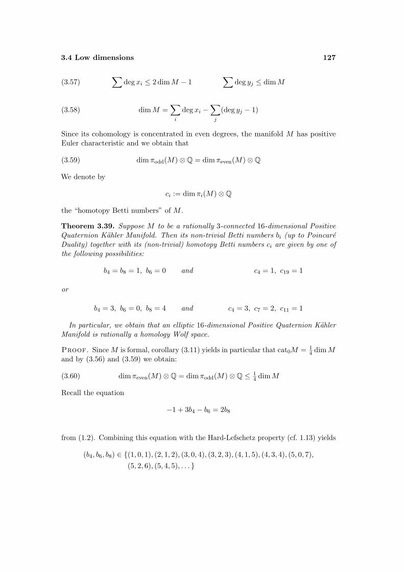
3.4 Low dimensions 127
∑deg xi ≤ 2 dimM − 1
∑deg yj ≤ dimM(3.57)
dimM =∑i
deg xi −∑j
(deg yj − 1)(3.58)
Since its cohomology is concentrated in even degrees, the manifold M has positiveEuler characteristic and we obtain that
dimπodd(M)⊗Q = dimπeven(M)⊗Q(3.59)
We denote by
ci := dimπi(M)⊗Q
the “homotopy Betti numbers” of M .
Theorem 3.39. Suppose M to be a rationally 3-connected 16-dimensional PositiveQuaternion Kahler Manifold. Then its non-trivial Betti numbers bi (up to PoincareDuality) together with its (non-trivial) homotopy Betti numbers ci are given by one ofthe following possibilities:
b4 = b8 = 1, b6 = 0 and c4 = 1, c19 = 1
or
b4 = 3, b6 = 0, b8 = 4 and c4 = 3, c7 = 2, c11 = 1
In particular, we obtain that an elliptic 16-dimensional Positive Quaternion KahlerManifold is rationally a homology Wolf space.
Proof. Since M is formal, corollary (3.11) yields in particular that cat0M = 14 dimM
and by (3.56) and (3.59) we obtain:
(3.60) dimπeven(M)⊗Q = dimπodd(M)⊗Q ≤ 14 dimM
Recall the equation
−1 + 3b4 − b6 = 2b8
from (1.2). Combining this equation with the Hard-Lefschetz property (cf. 1.13) yields
(b4, b6, b8) ∈ (1, 0, 1), (2, 1, 2), (3, 0, 4), (3, 2, 3), (4, 1, 5), (4, 3, 4), (5, 0, 7),(5, 2, 6), (5, 4, 5), . . .
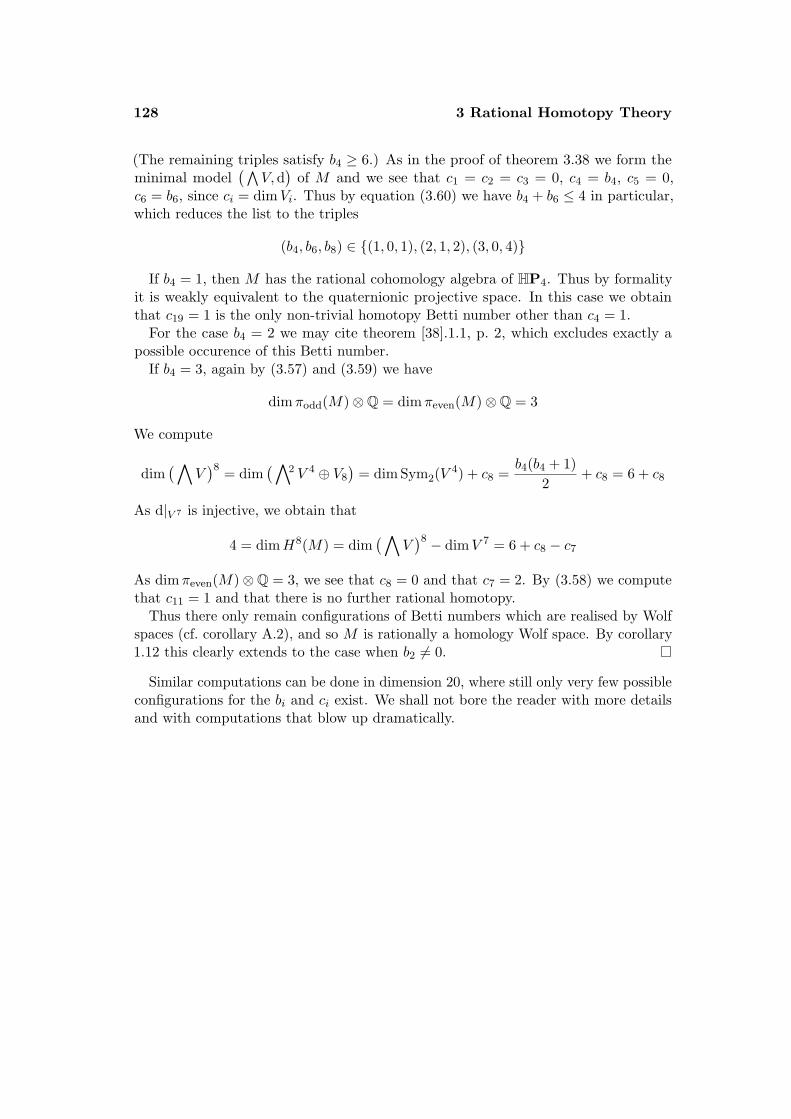
128 3 Rational Homotopy Theory
(The remaining triples satisfy b4 ≥ 6.) As in the proof of theorem 3.38 we form theminimal model
(∧V,d
)of M and we see that c1 = c2 = c3 = 0, c4 = b4, c5 = 0,
c6 = b6, since ci = dimVi. Thus by equation (3.60) we have b4 + b6 ≤ 4 in particular,which reduces the list to the triples
(b4, b6, b8) ∈ (1, 0, 1), (2, 1, 2), (3, 0, 4)
If b4 = 1, then M has the rational cohomology algebra of HP4. Thus by formalityit is weakly equivalent to the quaternionic projective space. In this case we obtainthat c19 = 1 is the only non-trivial homotopy Betti number other than c4 = 1.
For the case b4 = 2 we may cite theorem [38].1.1, p. 2, which excludes exactly apossible occurence of this Betti number.
If b4 = 3, again by (3.57) and (3.59) we have
dimπodd(M)⊗Q = dimπeven(M)⊗Q = 3
We compute
dim(∧
V)8 = dim
(∧2 V 4 ⊕ V8
)= dim Sym2(V 4) + c8 =
b4(b4 + 1)2
+ c8 = 6 + c8
As d|V 7 is injective, we obtain that
4 = dimH8(M) = dim(∧
V)8 − dimV 7 = 6 + c8 − c7
As dimπeven(M)⊗Q = 3, we see that c8 = 0 and that c7 = 2. By (3.58) we computethat c11 = 1 and that there is no further rational homotopy.
Thus there only remain configurations of Betti numbers which are realised by Wolfspaces (cf. corollary A.2), and so M is rationally a homology Wolf space. By corollary1.12 this clearly extends to the case when b2 6= 0.
Similar computations can be done in dimension 20, where still only very few possibleconfigurations for the bi and ci exist. We shall not bore the reader with more detailsand with computations that blow up dramatically.
4
Classification Results
In this chapter we combine several relations from Index Theory with the connectivitylemma, with further properties of Positive Quaternion Kahler Manifolds and with Lietheoretic arguments to obtain new properties of Positive Quaternion Kahler Manifoldsand partial classification results in low dimensions. By this we mainly refer to dimension20 beside dimensions 16 and 24.
Several arguments involve heavy computations. All of these were done with the helpof Mathematica 6.01 or Maple 9 or later programmme versions respectively.
4.1. Preparations
This section is devoted to a computation of several indices ip,q in terms of the char-acteristic numbers of the complexified tangent bundle TCM for a Positive QuaternionKahler Manifold M of dimension 20. That is, we compute
ip,q = 〈A(M) · ch(Rp,q),M〉
with Rp,q =∧p
0E ⊗ SqH as usual. For the analogous computations in dimension 16see chapter E of the appendix. The formulas relating these indices to other invariantsare given in theorem 1.17. For 5 + p+ q even they become:
ip,q =
0 for p+ q < 5(−1)p(b2p(M) + b2p−2(M) for p+ q = 5d for p = 0, q = 7
where d = dim Isom(M).Combining these equations with our computations yields the fundamental system of
equations we shall mainly be concerned with in the following sections. It is linear inthe characteristic numbers of M .
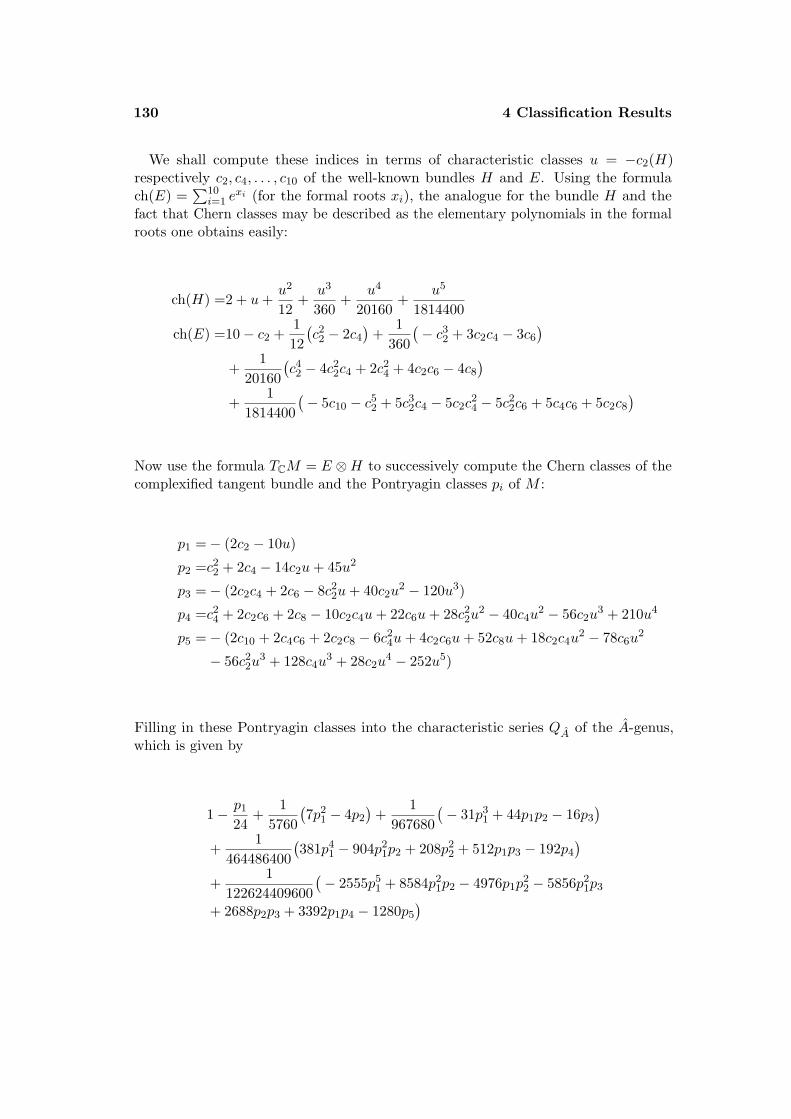
130 4 Classification Results
We shall compute these indices in terms of characteristic classes u = −c2(H)respectively c2, c4, . . . , c10 of the well-known bundles H and E. Using the formulach(E) =
∑10i=1 e
xi (for the formal roots xi), the analogue for the bundle H and thefact that Chern classes may be described as the elementary polynomials in the formalroots one obtains easily:
ch(H) =2 + u+u2
12+
u3
360+
u4
20160+
u5
1814400
ch(E) =10− c2 +112(c2
2 − 2c4
)+
1360
(− c3
2 + 3c2c4 − 3c6
)+
120160
(c4
2 − 4c22c4 + 2c2
4 + 4c2c6 − 4c8
)+
11814400
(− 5c10 − c5
2 + 5c32c4 − 5c2c
24 − 5c2
2c6 + 5c4c6 + 5c2c8
)
Now use the formula TCM = E ⊗H to successively compute the Chern classes of thecomplexified tangent bundle and the Pontryagin classes pi of M :
p1 =− (2c2 − 10u)
p2 =c22 + 2c4 − 14c2u+ 45u2
p3 =− (2c2c4 + 2c6 − 8c22u+ 40c2u
2 − 120u3)
p4 =c24 + 2c2c6 + 2c8 − 10c2c4u+ 22c6u+ 28c2
2u2 − 40c4u
2 − 56c2u3 + 210u4
p5 =− (2c10 + 2c4c6 + 2c2c8 − 6c24u+ 4c2c6u+ 52c8u+ 18c2c4u
2 − 78c6u2
− 56c22u
3 + 128c4u3 + 28c2u
4 − 252u5)
Filling in these Pontryagin classes into the characteristic series QA of the A-genus,which is given by
1− p1
24+
15760
(7p2
1 − 4p2
)+
1967680
(− 31p3
1 + 44p1p2 − 16p3
)+
1464486400
(381p4
1 − 904p21p2 + 208p2
2 + 512p1p3 − 192p4
)+
1122624409600
(− 2555p5
1 + 8584p21p2 − 4976p1p
22 − 5856p2
1p3
+ 2688p2p3 + 3392p1p4 − 1280p5
)
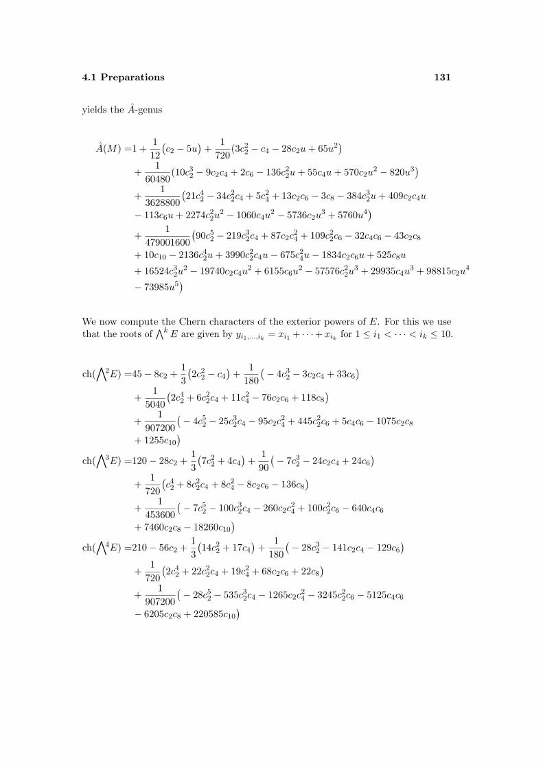
4.1 Preparations 131
yields the A-genus
A(M) =1 +112(c2 − 5u
)+
1720
(3c22 − c4 − 28c2u+ 65u2
)+
160480
(10c32 − 9c2c4 + 2c6 − 136c2
2u+ 55c4u+ 570c2u2 − 820u3
)+
13628800
(21c4
2 − 34c22c4 + 5c2
4 + 13c2c6 − 3c8 − 384c32u+ 409c2c4u
− 113c6u+ 2274c22u
2 − 1060c4u2 − 5736c2u
3 + 5760u4)
+1
479001600(90c5
2 − 219c32c4 + 87c2c
24 + 109c2
2c6 − 32c4c6 − 43c2c8
+ 10c10 − 2136c42u+ 3990c2
2c4u− 675c24u− 1834c2c6u+ 525c8u
+ 16524c32u
2 − 19740c2c4u2 + 6155c6u
2 − 57576c22u
3 + 29935c4u3 + 98815c2u
4
− 73985u5)
We now compute the Chern characters of the exterior powers of E. For this we usethat the roots of
∧k E are given by yi1,...,ik = xi1 + · · ·+ xik for 1 ≤ i1 < · · · < ik ≤ 10.
ch(∧
2E) =45− 8c2 +13(2c2
2 − c4
)+
1180
(− 4c3
2 − 3c2c4 + 33c6
)+
15040
(2c4
2 + 6c22c4 + 11c2
4 − 76c2c6 + 118c8
)+
1907200
(− 4c5
2 − 25c32c4 − 95c2c
24 + 445c2
2c6 + 5c4c6 − 1075c2c8
+ 1255c10
)ch(∧
3E) =120− 28c2 +13(7c2
2 + 4c4
)+
190(− 7c3
2 − 24c2c4 + 24c6
)+
1720
(c4
2 + 8c22c4 + 8c2
4 − 8c2c6 − 136c8
)+
1453600
(− 7c5
2 − 100c32c4 − 260c2c
24 + 100c2
2c6 − 640c4c6
+ 7460c2c8 − 18260c10
)ch(∧
4E) =210− 56c2 +13(14c2
2 + 17c4
)+
1180
(− 28c3
2 − 141c2c4 − 129c6
)+
1720
(2c4
2 + 22c22c4 + 19c2
4 + 68c2c6 + 22c8
)+
1907200
(− 28c5
2 − 535c32c4 − 1265c2c
24 − 3245c2
2c6 − 5125c4c6
− 6205c2c8 + 220585c10
)
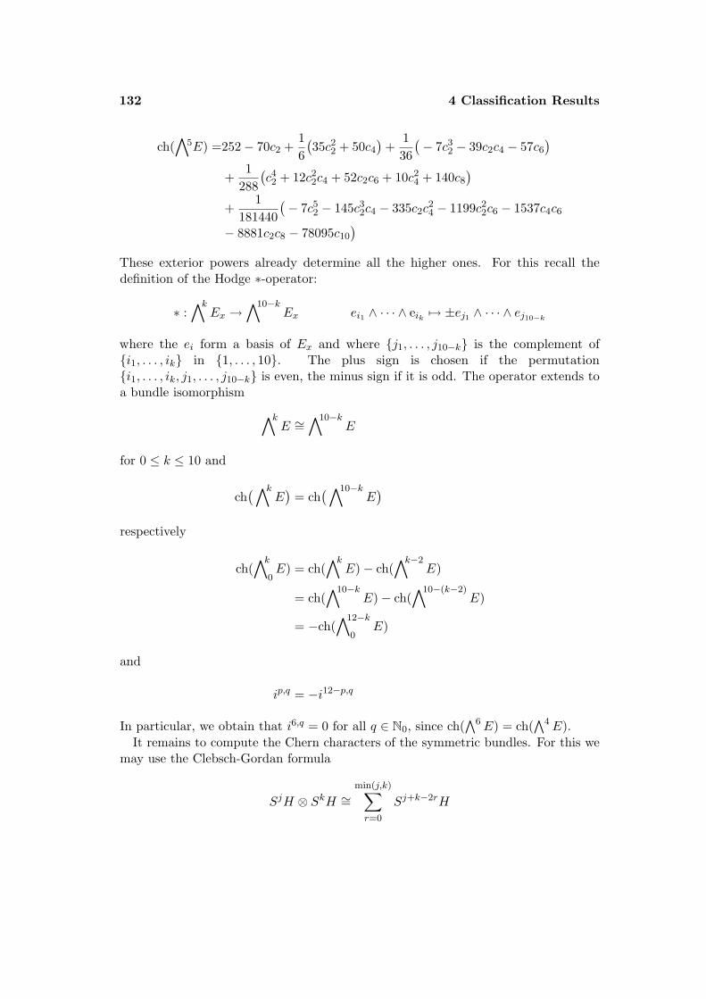
132 4 Classification Results
ch(∧
5E) =252− 70c2 +16(35c2
2 + 50c4
)+
136(− 7c3
2 − 39c2c4 − 57c6
)+
1288
(c4
2 + 12c22c4 + 52c2c6 + 10c2
4 + 140c8
)+
1181440
(− 7c5
2 − 145c32c4 − 335c2c
24 − 1199c2
2c6 − 1537c4c6
− 8881c2c8 − 78095c10
)These exterior powers already determine all the higher ones. For this recall thedefinition of the Hodge ∗-operator:
∗ :∧k
Ex →∧10−k
Ex ei1 ∧ · · · ∧ eik 7→ ±ej1 ∧ · · · ∧ ej10−k
where the ei form a basis of Ex and where j1, . . . , j10−k is the complement ofi1, . . . , ik in 1, . . . , 10. The plus sign is chosen if the permutationi1, . . . , ik, j1, . . . , j10−k is even, the minus sign if it is odd. The operator extends toa bundle isomorphism ∧k
E ∼=∧10−k
E
for 0 ≤ k ≤ 10 and
ch(∧k
E)
= ch(∧10−k
E)
respectively
ch(∧k
0E) = ch(
∧kE)− ch(
∧k−2E)
= ch(∧10−k
E)− ch(∧10−(k−2)
E)
= −ch(∧12−k
0E)
and
ip,q = −i12−p,q
In particular, we obtain that i6,q = 0 for all q ∈ N0, since ch(∧6E) = ch(
∧4E).It remains to compute the Chern characters of the symmetric bundles. For this we
may use the Clebsch-Gordan formula
SjH ⊗ SkH ∼=min(j,k)∑r=0
Sj+k−2rH
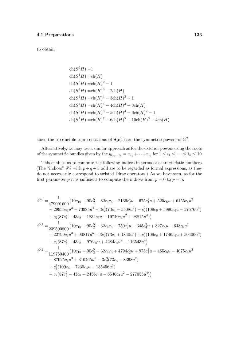
4.1 Preparations 133
to obtain
ch(S0H) =1
ch(S1H) =ch(H)
ch(S2H) =ch(H)2 − 1
ch(S3H) =ch(H)3 − 2ch(H)
ch(S4H) =ch(H)4 − 3ch(H)2 + 1
ch(S5H) =ch(H)5 − 4ch(H)3 + 3ch(H)
ch(S6H) =ch(H)6 − 5ch(H)4 + 6ch(H)2 − 1
ch(S7H) =ch(H)7 − 6ch(H)5 + 10ch(H)3 − 4ch(H)
since the irreducible representations of Sp(1) are the symmetric powers of C2.
Alternatively, we may use a similar approach as for the exterior powers using the rootsof the symmetric bundles given by the yi1,...,ik = xi1+· · ·+xik for 1 ≤ i1 ≤ · · · ≤ ik ≤ 10.
This enables us to compute the following indices in terms of characteristic numbers.(The “indices” ip,q with p+ q+ 5 odd are to be regarded as formal expressions, as theydo not necessarily correspond to twisted Dirac operators.) As we have seen, as for thefirst parameter p it is sufficient to compute the indices from p = 0 to p = 5.
i0,0 =1
479001600(10c10 + 90c5
2 − 32c4c6 − 2136c42u− 675c2
4u+ 525c8u+ 6155c6u2
+ 29935c4u3 − 73985u4 − 3c3
2(73c4 − 5508u2) + c22(109c6 + 3990c4u− 57576u3)
+ c2(87c24 − 43c8 − 1834c6u− 19740c4u
2 + 98815u4))
i0,1 =1
239500800(10c10 + 90c5
2 − 32c4c6 − 750c42u− 345c2
4u+ 327c8u− 643c6u2
− 22799c4u3 + 90817u5 − 3c3
2(73c4 + 1840u2) + c22(109c6 + 1746c4u+ 50400u3)
+ c2(87c24 − 43c8 − 976c6u+ 4284c4u
2 − 116543u4)
i0,3 =1
119750400(10c10 + 90c5
2 − 32c4c6 + 4794c42u+ 975c2
4u− 465c8u− 4075c6u2
+ 87025c4u3 + 310465u5 − 3c3
2(73c4 − 8368u2)
+ c22(109c6 − 7230c4u− 135456u3)
+ c2(87c24 − 43c8 + 2456c6u− 6540c4u
2 − 277055u4))
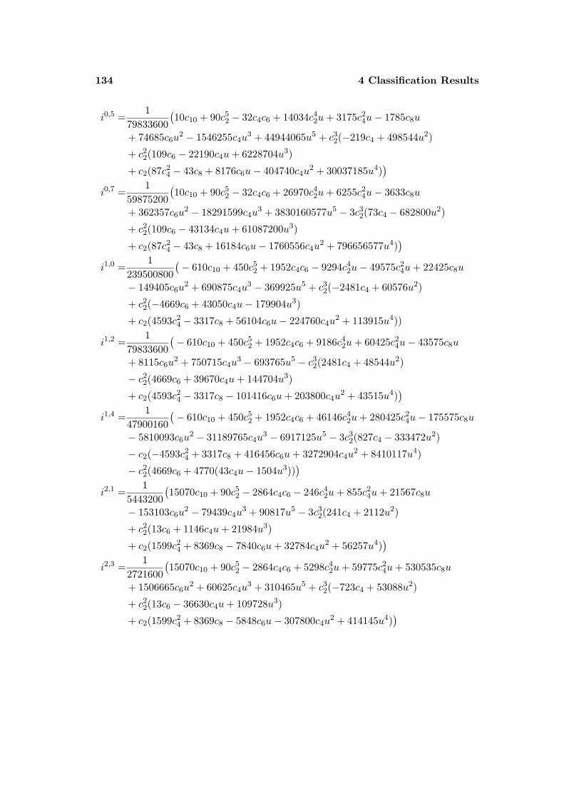
134 4 Classification Results
i0,5 =1
79833600(10c10 + 90c5
2 − 32c4c6 + 14034c42u+ 3175c2
4u− 1785c8u
+ 74685c6u2 − 1546255c4u
3 + 44944065u5 + c32(−219c4 + 498544u2)
+ c22(109c6 − 22190c4u+ 6228704u3)
+ c2(87c24 − 43c8 + 8176c6u− 404740c4u
2 + 30037185u4))
i0,7 =1
59875200(10c10 + 90c5
2 − 32c4c6 + 26970c42u+ 6255c2
4u− 3633c8u
+ 362357c6u2 − 18291599c4u
3 + 3830160577u5 − 3c32(73c4 − 682800u2)
+ c22(109c6 − 43134c4u+ 61087200u3)
+ c2(87c24 − 43c8 + 16184c6u− 1760556c4u
2 + 796656577u4))
i1,0 =1
239500800(− 610c10 + 450c5
2 + 1952c4c6 − 9294c42u− 49575c2
4u+ 22425c8u
− 149405c6u2 + 690875c4u
3 − 369925u5 + c32(−2481c4 + 60576u2)
+ c22(−4669c6 + 43050c4u− 179904u3)
+ c2(4593c24 − 3317c8 + 56104c6u− 224760c4u
2 + 113915u4))
i1,2 =1
79833600(− 610c10 + 450c5
2 + 1952c4c6 + 9186c42u+ 60425c2
4u− 43575c8u
+ 8115c6u2 + 750715c4u
3 − 693765u5 − c32(2481c4 + 48544u2)
− c22(4669c6 + 39670c4u+ 144704u3)
+ c2(4593c24 − 3317c8 − 101416c6u+ 203800c4u
2 + 43515u4))
i1,4 =1
47900160(− 610c10 + 450c5
2 + 1952c4c6 + 46146c42u+ 280425c2
4u− 175575c8u
− 5810093c6u2 − 31189765c4u
3 − 6917125u5 − 3c32(827c4 − 333472u2)
− c2(−4593c24 + 3317c8 + 416456c6u+ 3272904c4u
2 + 8410117u4)
− c22(4669c6 + 4770(43c4u− 1504u3))
)i2,1 =
15443200
(15070c10 + 90c5
2 − 2864c4c6 − 246c42u+ 855c2
4u+ 21567c8u
− 153103c6u2 − 79439c4u
3 + 90817u5 − 3c32(241c4 + 2112u2)
+ c22(13c6 + 1146c4u+ 21984u3)
+ c2(1599c24 + 8369c8 − 7840c6u+ 32784c4u
2 + 56257u4))
i2,3 =1
2721600(15070c10 + 90c5
2 − 2864c4c6 + 5298c42u+ 59775c2
4u+ 530535c8u
+ 1506665c6u2 + 60625c4u
3 + 310465u5 + c32(−723c4 + 53088u2)
+ c22(13c6 − 36630c4u+ 109728u3)
+ c2(1599c24 + 8369c8 − 5848c6u− 307800c4u
2 + 414145u4))
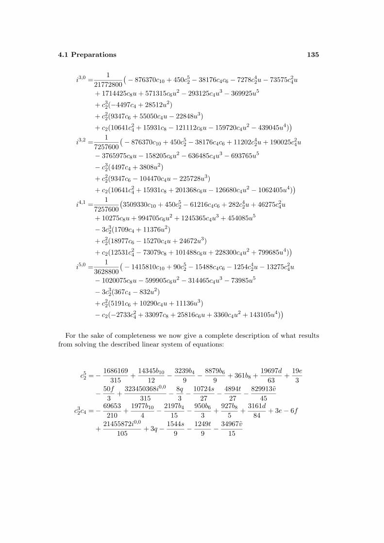
4.1 Preparations 135
i3,0 =1
21772800(− 876370c10 + 450c5
2 − 38176c4c6 − 7278c42u− 73575c2
4u
+ 1714425c8u+ 571315c6u2 − 293125c4u
3 − 369925u5
+ c32(−4497c4 + 28512u2)
+ c22(9347c6 + 55050c4u− 22848u3)
+ c2(10641c24 + 15931c8 − 121112c6u− 159720c4u
2 − 439045u4))
i3,2 =1
7257600(− 876370c10 + 450c5
2 − 38176c4c6 + 11202c42u+ 190025c2
4u
− 3765975c8u− 158205c6u2 − 636485c4u
3 − 693765u5
− c32(4497c4 + 3808u2)
+ c22(9347c6 − 104470c4u− 225728u3)
+ c2(10641c24 + 15931c8 + 201368c6u− 126680c4u
2 − 1062405u4))
i4,1 =1
7257600(3509330c10 + 450c5
2 − 61216c4c6 + 282c42u+ 46275c2
4u
+ 10275c8u+ 994705c6u2 + 1245365c4u
3 + 454085u5
− 3c32(1709c4 + 11376u2)
+ c22(18977c6 − 15270c4u+ 24672u3)
+ c2(12531c24 − 73079c8 + 101488c6u+ 228300c4u
2 + 799685u4))
i5,0 =1
3628800(− 1415810c10 + 90c5
2 − 15488c4c6 − 1254c42u− 13275c2
4u
− 1020075c8u− 599905c6u2 − 314465c4u
3 − 73985u5
− 3c32(367c4 − 832u2)
+ c22(5191c6 + 10290c4u+ 11136u3)
− c2(−2733c24 + 33097c8 + 25816c6u+ 3360c4u
2 + 143105u4))
For the sake of completeness we now give a complete description of what resultsfrom solving the described linear system of equations:
c52 =− 1686169
315+
14345b10
12− 3239b4
9− 8879b6
9+ 361b8 +
19697d63
+19e3
− 50f3
+323450368i0,0
315− 8q
3− 10724s
27− 4894t
27− 829913v
45
c32c4 =− 69653
210+
1977b10
4− 2197b4
15− 950b6
3+
927b85
+3161d
84+ 3e− 6f
+21455872i0,0
105+ 3q − 1544s
9− 1249t
9− 34967v
15
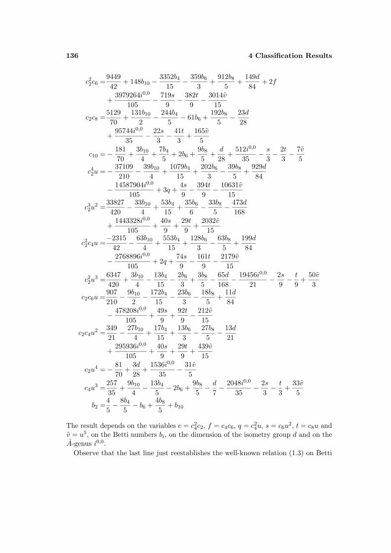
136 4 Classification Results
c22c6 =
944942
+ 148b10 −3352b4
15− 359b6
3+
912b85
+149d84
+ 2f
+3979264i0,0
105− 719s
9− 382t
9− 3014v
15
c2c8 =512970
+131b10
2− 244b4
5− 61b6 +
192b85− 23d
28
+95744i0,0
35− 22s
3− 41t
3+
165v5
c10 =− 18170
+3b10
4+
7b45
+ 2b6 +9b85
+d
28+
512i0,0
35− s
3− 2t
3− 7v
5
c42u =− 37109
210− 39b10
4+
1079b415
+202b6
3− 39b8
5+
929d84
− 14587904i0,0
105+ 3q +
4s9− 394t
9− 10631v
15
c32u
2 =33827420
− 33b10
4+
53b415
+35b6
6− 33b8
5− 473d
168
+1443328i0,0
105+
40s9
+29t9
+2032v
15
c22c4u =
−231542
− 63b10
4+
553b415
+128b6
3− 63b8
5+
199d84
− 2768896i0,0
105+ 2q +
74s9− 161t
9− 2179v
15
c22u
3 =6347420
+3b10
4− 13b4
15− 2b6
3+
3b85− 65d
168− 19456i0,0
21− 2s
9− t
9+
50v3
c2c6u =907210− 9b10
2− 172b4
15− 23b6
3− 18b8
5+
11d84
− 478208i0,0
105+
49s9
+92t9− 212v
15
c2c4u2 =
34921− 27b10
4+
17b415
+13b6
3− 27b8
5− 13d
21
+295936i0,0
105+
40s9
+29t9
+439v15
c2u4 =− 81
70+
3d28
+1536i0,0
35− 31v
5
c4u3 =
25735
+9b10
4− 13b4
5− 2b6 +
9b85− d
7− 2048i0,0
35− 2s
3− t
3+
33v5
b2 =45− 8b4
5− b6 +
4b85
+ b10
The result depends on the variables e = c24c2, f = c4c6, q = c2
4u, s = c6u2, t = c8u and
v = u5, on the Betti numbers bi, on the dimension of the isometry group d and on theA-genus i0,0.
Observe that the last line just reestablishes the well-known relation (1.3) on Betti
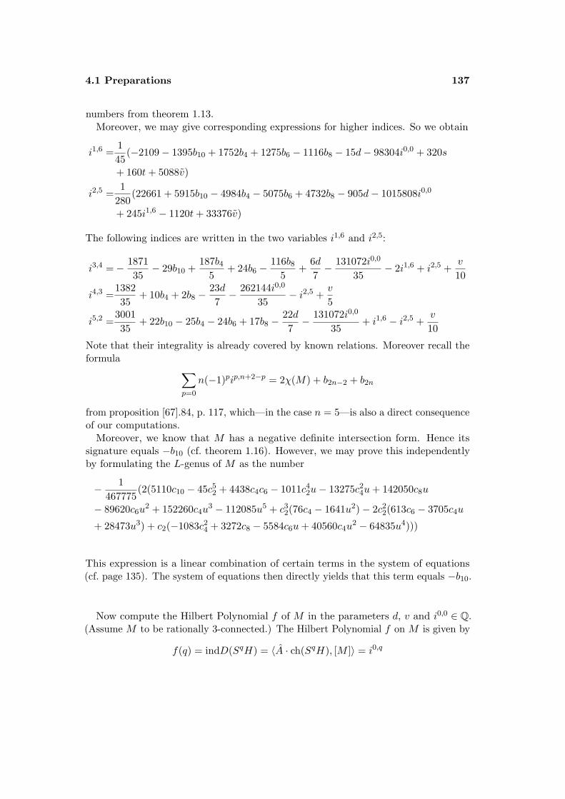
4.1 Preparations 137
numbers from theorem 1.13.Moreover, we may give corresponding expressions for higher indices. So we obtain
i1,6 =145
(−2109− 1395b10 + 1752b4 + 1275b6 − 1116b8 − 15d− 98304i0,0 + 320s
+ 160t+ 5088v)
i2,5 =1
280(22661 + 5915b10 − 4984b4 − 5075b6 + 4732b8 − 905d− 1015808i0,0
+ 245i1,6 − 1120t+ 33376v)
The following indices are written in the two variables i1,6 and i2,5:
i3,4 =− 187135− 29b10 +
187b45
+ 24b6 −116b8
5+
6d7− 131072i0,0
35− 2i1,6 + i2,5 +
v
10
i4,3 =138235
+ 10b4 + 2b8 −23d7− 262144i0,0
35− i2,5 +
v
5
i5,2 =300135
+ 22b10 − 25b4 − 24b6 + 17b8 −22d7− 131072i0,0
35+ i1,6 − i2,5 +
v
10
Note that their integrality is already covered by known relations. Moreover recall theformula ∑
p=0
n(−1)pip,n+2−p = 2χ(M) + b2n−2 + b2n
from proposition [67].84, p. 117, which—in the case n = 5—is also a direct consequenceof our computations.
Moreover, we know that M has a negative definite intersection form. Hence itssignature equals −b10 (cf. theorem 1.16). However, we may prove this independentlyby formulating the L-genus of M as the number
− 1467775
(2(5110c10 − 45c52 + 4438c4c6 − 1011c4
2u− 13275c24u+ 142050c8u
− 89620c6u2 + 152260c4u
3 − 112085u5 + c32(76c4 − 1641u2)− 2c2
2(613c6 − 3705c4u
+ 28473u3) + c2(−1083c24 + 3272c8 − 5584c6u+ 40560c4u
2 − 64835u4)))
This expression is a linear combination of certain terms in the system of equations(cf. page 135). The system of equations then directly yields that this term equals −b10.
Now compute the Hilbert Polynomial f of M in the parameters d, v and i0,0 ∈ Q.(Assume M to be rationally 3-connected.) The Hilbert Polynomial f on M is given by
f(q) = indD(SqH) = 〈A · ch(SqH), [M ]〉 = i0,q
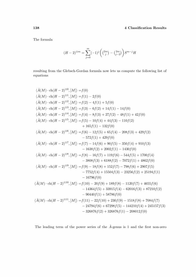
138 4 Classification Results
The formula
(H − 2)⊗m =m∑j=0
(−1)j((
2mj
)−(
2mj−2
))Sm−jH
resulting from the Glebsch-Gordan formula now lets us compute the following list ofequations
〈A(M) · ch(H − 2)⊗0, [M ]〉 =f(0)
〈A(M) · ch(H − 2)⊗1, [M ]〉 =f(1)− 2f(0)
〈A(M) · ch(H − 2)⊗2, [M ]〉 =f(2)− 4f(1) + 5f(0)
〈A(M) · ch(H − 2)⊗3, [M ]〉 =f(3)− 6f(2) + 14f(1)− 14f(0)
〈A(M) · ch(H − 2)⊗4, [M ]〉 =f(4)− 8f(3) + 27f(2)− 48f(1) + 42f(0)
〈A(M) · ch(H − 2)⊗5, [M ]〉 =f(5)− 10f(4) + 44f(3)− 110f(2)+ 165f(1)− 132f(0)
〈A(M) · ch(H − 2)⊗6, [M ]〉 =f(6)− 12f(5) + 65f(4)− 208f(3) + 429f(2)− 572f(1) + 429f(0)
〈A(M) · ch(H − 2)⊗7, [M ]〉 =f(7)− 14f(6) + 90f(5)− 350f(4) + 910f(3)− 1638f(2) + 2002f(1)− 1430f(0)
〈A(M) · ch(H − 2)⊗8, [M ]〉 =f(8)− 16f(7) + 119f(6)− 544f(5) + 1700f(4)− 3808f(3) + 6188f(2)− 7072f(1) + 4862f(0)
〈A(M) · ch(H − 2)⊗9, [M ]〉 =f(9)− 18f(8) + 152f(7)− 798f(6) + 2907f(5)− 7752f(4) + 15504f(3)− 23256f(2) + 25194f(1)− 16796f(0)
〈A(M) · ch(H − 2)⊗10, [M ]〉 =f(10)− 20f(9) + 189f(8)− 1120f(7) + 4655f(6)− 14364f(5) + 33915f(4)− 62016f(3) + 87210f(2)− 90440f(1) + 58786f(0)
〈A(M) · ch(H − 2)⊗11, [M ]〉 =f(11)− 22f(10) + 230f(9)− 1518f(8) + 7084f(7)− 24794f(6) + 67298f(5)− 144210f(4) + 245157f(3)− 326876f(2) + 326876f(1)− 208012f(0)
The leading term of the power series of the A-genus is 1 and the first non-zero
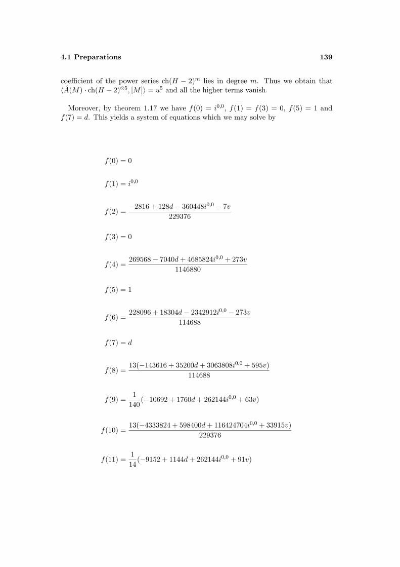
4.1 Preparations 139
coefficient of the power series ch(H − 2)m lies in degree m. Thus we obtain that〈A(M) · ch(H − 2)⊗5, [M ]〉 = u5 and all the higher terms vanish.
Moreover, by theorem 1.17 we have f(0) = i0,0, f(1) = f(3) = 0, f(5) = 1 andf(7) = d. This yields a system of equations which we may solve by
f(0) = 0
f(1) = i0,0
f(2) =−2816 + 128d− 360448i0,0 − 7v
229376
f(3) = 0
f(4) =269568− 7040d+ 4685824i0,0 + 273v
1146880
f(5) = 1
f(6) =228096 + 18304d− 2342912i0,0 − 273v
114688
f(7) = d
f(8) =13(−143616 + 35200d+ 3063808i0,0 + 595v)
114688
f(9) =1
140(−10692 + 1760d+ 262144i0,0 + 63v)
f(10) =13(−4333824 + 598400d+ 116424704i0,0 + 33915v)
229376
f(11) =114
(−9152 + 1144d+ 262144i0,0 + 91v)
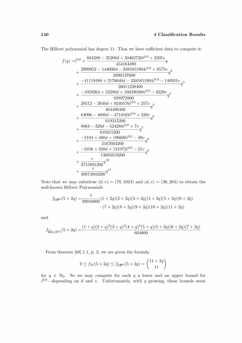
140 4 Classification Results
The Hilbert polynomial has degree 11. Thus we have sufficient data to compute it:
f(q) =i0,0 +684288− 35200d+ 50462720i0,0 + 2205v
454164480q
+2909952− 144000d− 3385851904i0,0 + 8575v
2890137600q2
+−41119488 + 2176640d− 3385851904i0,0 − 140931v
26011238400q3
+−1059264 + 53280d+ 166330368i0,0 − 3229v
928972800q4
+28512− 2640d+ 9240576i0,0 + 257v
464486400q5
+84096− 4800d− 4718592i0,0 + 329v
619315200q6
+8064− 320d− 524288i0,0 + 7v
619315200q7
+−5184 + 480d+ 196608i0,0 − 49v
2167603200q8
+−3456 + 320d+ 131072i0,0 − 21v
13005619200q9
+v
3715891200q10
+v
40874803200q11
Note that we may substitue (d, v) = (78, 1024) and (d, v) = (36, 264) to obtain thewell-known Hilbert Polynomials
fHP5(5 + 2q) =1
39916800(1 + 2q)(2 + 2q)(3 + 2q)(4 + 2q)(5 + 2q)(6 + 2q)
· (7 + 2q)(8 + 2q)(9 + 2q)(10 + 2q)(11 + 2q)
and
fGr4(R9)
(5 + 2q) =(1 + q)(2 + q)2(3 + q)2(4 + q)2(5 + q)(5 + 2q)(6 + 2q)(7 + 2q)
604800
From theorem [68].1.1, p. 2, we are given the formula
0 ≤ fM (5 + 2q) ≤ fHP5(5 + 2q) =(
11 + 2q11
)for q ∈ N0. So we may compute for each q a lower and an upper bound fori0,0—depending on d and v. Unfortunately, with q growing, these bounds seem

4.2 Recognising quaternionic projective spaces 141
to become worse so that we use low values of q—i.e. q = 3 respectively q = 2—toobtain:
114
(−9152 + 262144i0,0 + 1144d+ 91v) ≤ 12376(4.1)
1140
(−10692 + 262144i0,0 + 1760d+ 63v) ≥ 0(4.2)
Unfortunately, these inequalities are not strong enough to yield the vanishing of the A-genus (when filing in the known bounds for d and v). Observe that from the integralityof indices used in the Hilbert polynomial or from the integrality of Pontryagin classesone may deduce certain properties on divisibility which, however, do not seem to bestrong enough to make essential progress on the topic.
Let us now compute further relations involving the A-genus of a Positive QuaternionKahler Manifold M . We adapt lemma [66].7.6, p. 169, to dimension 20 and plug inthe expression −(2c2 − 10u) for the first Pontryagin class p1:
8u5 − p1u4 ≥ 0⇔ 8u5 + (2c2 − 10u)u4 ≥ 0⇔ c2u
4 − u5 ≥ 0(4.3)
From the solution of the fundamental system of equations (cf. page 135) we cite
c2u4 = −81
70+
3d28
+1536A(M)[M ]
35− 31u5
5
Combining it with formula (4.3) yields
−8170
+3d28− 36u5
5+
1536A(M)[M ]35
≥ 0(4.4)
Recall that 1 ≤ v ≤ 1024. So for d = 0 the equation becomes
−8170− 36
5 · 1024+
1536A(M)[M ]35
≥ 0(4.5)
4.2. Recognising quaternionic projective spaces
In this section we shall prove recognition theorems of the following kind: Wheneverthe fourth Betti number of a Positive Quaternion Kahler Manifold M equals one, thenM is homothetic to the quaternionic projective space.
This theorem is well-known in dimensions smaller than or equal to 16—cf. 1.15. Weshall generalise it to dimensions 20 and 24. We remark that a general theorem of this
142 4 Classification Results
kind cannot hold true, since the exceptional Wolf spaces equally satisfy b4 = 1—cf. theremark on [67], p. 89. Nonetheless, as we were told by Gregor Weingart, in dimension28 a similar recognition theorem—which also identifies the exceptional Wolf spaceF4/Sp(3)Sp(1)—seems to be possible.
Let us first give generalisations of the theorem in dimension 16.
4.2.1. Dimension 16
In dimension 16 the relations on Betti numbers given in (1.2) of theorem 1.13 togetherwith the Hard-Lefschetz property have the following consequence: If b4 = 1 and if we as-sume M to be rationally 3-connected (cf. 1.12), we obtainb0 = b4 = b8 = b12 = b16 = 1 with all the other Betti numbers vanishing. Sonecessarily every Pontryagin class is a multiple of the corresponding power of the formu. This motivates the following slight improvement.
Proposition 4.1. If each of the Chern classes ci of the bundle E over a 16-dimensionalPositive Quaternion Kahler Manifold is a (scalar) multiple of the corresponding powerof u, then the manifold already is homothetic to HP4.
Proof. We refer the reader to chapter E of the appendix for the computation of allthe necessary indices ip,q in dimension 16. We then may form the system of equationsas in 1.17. This system is linear in the characteristic numbers.
By assumption we may now replace every Chern class ci by some xiuni for xi ∈ R.If one focuses on the case b2 = 0 (cf. 1.12), the system of equations can be solved
and it yields d = 55, b4 = b8 = 1, b6 = 0, u4 = 1 (with all the factors xi equal to one).We then observe that in dimension 55 only semi-simple Lie groups of rank at least 5appear. Theorem 1.18 then yields the assertion; i.e. the isometry group becomes verylarge and permits to identify M as the quaternionic projective space.
If one does not assume b2 = 0, the list of possible configurations for(d, b2, b4, b6, b8, u4) becomes a little larger. However, the configuration from aboveremains the only one with integral d ∈ Z.
Assume b2 = 0. Then the same proof works if one only requires c2 and c4 to bescalar multiples of u respectively u2. In this case a numerical solving procedure leadsto six different solutions of which the only one with an integral value for d is therequested one as in proposition 4.1.
Focussing on the case that only c2 is a multiple x ∈ R of u leads to the two equations
d = 7 +v
6+vx
48(4.6)
b4 =7832− 7
8v − 9
16vx− 11
128vx2 − 1
512vx3(4.7)
where v = (4u)4 is the quaternionic volume. The element x is integral by the samereasoning as in the original proof, i.e. the proof of theorem [28].5.1, p. 62. On page 21
4.2 Recognising quaternionic projective spaces 143
we saw that it is plausible to suppose the vanishing of i1,5 in the case M 6= HP4. Thisassumption produces
d =7(304 + 56x+ 3x2)
16 + 20x+ 3x2(4.8)
b4 =− 27(1280− 304x− 40x2 + 7x3)8(16 + 20x+ 3x2)
(4.9)
b6 =136(3289− 294x+ 63x2 − 6(c4u
2)x2 − 5320016 + 20x+ 3x2
(4.10)
− 93548x16 + 20x+ 3x2
)b8 =
1144
(14410− 1113x− (126x2 − 12(c4u
2))x2 − 116368016 + 20x+ 3x2
(4.11)
+14728x
16 + 20x+ 3x2
)c2
4 =116
(− 3546 + 567x− 378x2 + 44(c4u
2)x2 − 82152016 + 20x+ 3x2
(4.12)
+445032x
16 + 20x+ 3x2
)The only integral solution for 8 ≤ d < 55 = dim Sp(5) (cf. theorem 1.18) is given byx = 4 and d = 28. Then we directly obtain b4 = 3 by (4.9) and also v = 84 by (4.6).Indeed, by the relations on Betti numbers in 1.13 only two possibilities for (b4, b6, b8)remain, namely (3, 0, 4) or (3, 2, 3). Equations (4.10) and (4.11) yield c4u
2 = 2732 in
the first case. By theorem 1.16 we may use the positive definiteness of the bilinearform Q to see 0 ≤ Q(c4, c4) = c2
4. Yet, in the case (b4, b6, b8) = (3, 2, 3) we obtain thecontradiction c2
4 = −7516 by (4.12). As a consequence, we have the following theorem:
Theorem 4.2. If M is a rationally 3-connected 16-dimensional Positive QuaternionKahler Manifold with i1,5 = 0 and if the class c2 is a scalar multiple of u, then eitherM ∼= HP4 or the datum (d, v, b4, b6, b8) = (28, 84, 3, 0, 4) is exactly the one of Gr4(R8).
We remark that the property that c2 is a multiple of u seems to be a special featureof Gr4(Rn+4) for n = 4 among the infinite series of Wolf spaces other than thequaternionic projective space.
4.2.2. Dimension 20
Let us now prove the result in dimension 20. Again, without restriction we focus onrationally 3-connected Positive Quaternion Kahler Manifolds M20—cf. 1.12.
144 4 Classification Results
Theorem 4.3. If each of the Chern classes c2i of E over M is a (scalar) multiple ofthe corresponding power of u, then M ∼= HP5.
Proof. We proceed as before in dimension 16; i.e. we solve the system of equations(cf. page 135) setting all characteristic classes to rational multiples of a suitable powerof the form u. As a result we obtain b4 = b8 = 1, b6 = b10 = 0, u5 = 1, all thescalars are 1 and d = 78. However, such a large isometry group can only occur for thequaternionic projective space—cf. theorem 1.18.
We remark that for this proof to work we do not need that c6 is a scalar multiple ofu3. We shall now use the observation we stated in lemma 1.14 to finish the reasoning.
Corollary 4.4. If b4(M20) = 1, then M20 ∼= HP5.
Proof. Lemma 1.14 tells us that b4 = 1 implies b8 = 1. By Poincare Duality we mayconclude that all the c2i ∈ H4i(M) satisfy the condition from theorem 4.3.
Observe that clearly by this corollary we have ruled out an infinite number ofpossible configurations of Betti numbers, since it automatically follows that b4 = 1 notonly implies b8 = 1 but also b6 = b10 = 0.
Observe that one may prove this corollary in a slightly different way: Assume onlythat c2 and u are scalar multiples and do the same for monomials containing c2 and u.Use the equations with the additional information b4 = 1 (and b2 = 0) and the resultfollows directly.
4.2.3. Dimension 24
We apply similar techniques as before to prove
Theorem 4.5. A 24-dimensional Positive Quaternion Kahler Manifold M withb4(M) = 1 is homothetic to HPn.
Proof. Again we replace c2 by a scalar multiple of u and do the same for all themonomials containing c2 as a factor. This and the additional information b4 = 1(respectively b2 = 0) simplifies the system of equations (cf. 1.17) that we build up aswe did for dimensions 16 and 20. Solving it yields a list of possibilities, which we runthrough in order to isolate the one leading to HP6:
We may rule out the first solution, since it yields d = 2447242891 6∈ Z for the dimension of
the isometry group. The second solution gives d = 105 = dim Sp(7). Thus we directlyknow that M ∼= HP6 in this case—cf. theorem 1.18. So what is left is to rule out thefollowing configuration of solutions, which is marked by
d =7937019926774969402874803650560
x1 −195921969594057972417248821903360
x22 +
4574522790965369092417248821903360
− 263256496233805749607301120
x63 +
1176648936457402874803650560
x54 +
14142811929437161149921460224
x45
− 282904843313851604312205475840
x36
4.3 Properties of interest 145
where each xi is a root of
29223x7 − 358275x6 − 6960405x5 + 67759961x4 + 579930789x3 − 4142432537x2
− 9711667063x+ 33284884867
Numerically, the roots of this polynomial are given by
2.156753156, 7.720829360, 11.12408307, 15.23992325,−10.15093795 + 2.570319306i,− 3.679678028,−10.15093795− 2.570319306i
A computer-based check on all the possible combinations now shows that there are nointegral solutions for d in all these cases. So we are done.
4.3. Properties of interest
In this section we shall show that under slight assumptions some surprising resultson the degree of symmetry of 20-dimensional Positive Quaternion Kahler Manifoldsare obtained.
Proposition 4.6. Unless M20 admits an isometric S1-action, the A-genus of M20 isrestricted by
0.0321350097 < A(M)[M ] < 0.6955146790
Proof. The upper bound clearly results from equation (4.1) when substituting inthe extremal value v = 1. For the lower bound we form the linear combination
1448
(−1053 + 136d+ 32768i0,0) ≥ 0
out of equations (4.2) and (4.4). Plug in d = 0 and the result follows.
Let us now use the fact that the terms f(5 + 2q) = i0,5+2q (for q ≥ 0) are indices ofthe twisted Dirac operator D/(S5+2qH); i.e. in particular they are integral. This leadsto congruence relations for the dimension of the isometry group and the quaternionicvolume.
Theorem 4.7. A 20-dimensional rationally 3-connected Positive Quaternion KahlerManifold with A(M)[M ] = 0 satisfies
d ≡ 1 mod 7 and v ≡ 4 mod 20
146 4 Classification Results
Proof. We use the Hilbert Polynomial f of M . Thus, using the assumption thatA(M)[M ] = 0, we obtain
Z 3 i0,9 = f(9) =1
140(−10692 + 1760d+ 63v).
This implies that
− 10692 + 1760d+ 63v ≡ 0 mod 140⇐⇒ 88 + 80d+ 63v ≡ 0 mod 140⇐⇒ (d ≡ 1 mod 7) ∨ (v ≡ 4 mod 20)
Remark 4.8. • Any computation of further indices seems to result in the factthat only denominators appear that divide 22 · 5 · 7. Since vHP5 = 1024 andsince v
Gr4(R9)= 264, we see that the relations found in the theorem are the only
ones that may hold on the quaternionic volume when focussing on congruencemodulo m for m|140.
• The dimension dHPn of HPn is given by (n+ 1)(2n+ 3) with
dHPn ≡ (n+ 1)((n+ 1) + (n+ 2)) ≡ (−1)(−1 + 0) ≡ 1 mod n+ 2.
The dimension dGr4(Rn+4)
of Gr4(Rn+4) is given by
dGr4(Rn+4)
=
((n+ 3)/2)(2(n+ 3)/2 + 1) = 1
2(n+ 3)(n+ 4) for n odd((n+ 4)/2)(2(n+ 4)/2− 1) = 1
2(n+ 3)(n+ 4) for n even
So in any case we have
dGr4(Rn+4)
≡ 12· 1 · 2 ≡ 1 mod n+ 2.
Thus in dimensions without exceptional Wolf spaces—for these it is not true—bythe main conjecture 1.6 it should hold on a rationally 3-connected Positive Quater-nion Kahler Manifold that the dimension of the isometry group is congruent 1modulo n+ 2.
Corollary 4.9. A 20-dimensional Positive Quaternion Kahler Manifold satisfyingA(M)[M ] = 0 and possessing an isometry group of dimension greater than 36 isisometric to the complex Grassmannian or the quaternionic projective space.
Proof. By corollary 1.12 we assume the manifold to be rationally 3-connected. Thereare no compact Lie groups in dimensions 43, 50, 57, 64 and 71 with rank smaller thanor equal to 5. Thus theorems 1.18 and 4.7 yield the result.
4.3 Properties of interest 147
We shall now prove the existence of S1-actions on 20-dimensional Positive QuaternionKahler Manifolds which satisfy some slight assumptions. For this we use the definitenessof the intersection form to establish
Lemma 4.10. We have:
u5 ≥ 0 c42u ≥ 0 c2
2u3 ≥ 0 c2
4u ≥ 0
More generally, the same holds for
(kc22 + lc2u+mu2 + nc4)2u ≥ 0
with k, l,m, n ∈ R.
Proof. Recall the generalised intersection form Q from theorem 1.16. All the classesy from the assertion may be written as y = Q(x, x) for some x ∈ Hr(M) with r ∈ 4, 8.However, the intersection form Q is positive definite in degrees divisible by 4 and itresults that Q(x, x) ≥ 0.
Lemma 4.10 yields that c22u
3 ≥ 0, which translates to
495392− 14240d− 35651584i0,0 − 1120i1,6 + 707v35840
≥ 0
after solving the usual system of equations on indices (cf. page 135) and substitutingin the special solution for i1,6. So we obtain:
i1,6 ≤ 495392− 14240d− 35651584i0,0 + 707v1120
which already shows that for extremal values of v and d, i.e. v = 1024 and d = 0, theindex i1,6 becomes very small.
Now consider the term (c2u + mu2)2u together with the solution from the sys-tem of equations (cf. page 135) and the solution for i1,6. By lemma 4.10 we have(c2u+mu2)2u ≥ 0. Suppose d = 0. This has the consequence that
i1,6 ≤ 495392− 35651584i0,0 − 82944m+ 3145728i0,0m+ 707v − 434mv + 35m2v
1120
for all m ∈ R. The right hand side is a parabola in m. Determine the apex of thisparabola as m0 = 41472−1572864i0,0+217v
35v , put it into the inequality and obtain:
i1,6 ≤ − 14900v
(214990848 + 309237645312(i0,0)2 + 82516v + 2793v2
+ 131072i0,0(−124416 + 539v))
The right hand side is a function in i0,0 and v which has no critical point in the interiorof the square
[0.0321350097, 0.695514790
]×[1, 1024
]—cf. proposition 4.6. Thus its
148 4 Classification Results
maximum lies in the boundary of the square. A direct check reveals that on theborder of the square the function is decreasing monotonously in i0,0 for v ∈ 1, 1024.Analogously, we see that for i0,0 = 0.0321350097 the function has the only maximum−549.348 for v = 61 and for i0,0 = 0.695514790 it is increasing in [1, 1024]. So ittakes its maximum −549.348 on the square in v = 61 and i0,0 = 0.695514790. So, inparticular, we obtain the following theorem:
Theorem 4.11. A 20-dimensional Positive Quaternion Kahler Manifold with
i1,6 ≥ −549
admits an effective isometric S1-action.
As we explained on page 21, for M 6∼= HPn the index i1,6 is smaller or equal to zeroand it is conjectured to equal zero. On HPn it equals i1,n+1 = n(2n+ 3).
Next we shall link the existence of an isometric S1-action to the Euler characteristic.
Theorem 4.12. A 20-dimensional Positive Quaternion Kahler Manifold M withEuler characteristic restricted by
χ(M) < 16236
admits an effective isometric S1-action. The same holds if the Betti numbers of Msatisfy either
b4 −b64< 842.5
or
59b43− 25b6
4< 3027.93
or—as a combination of both inequalities—if
b4 ≤ 3381
Proof. The theorem is trivial for Gr2(C7). Thus by 1.12 we assume M to be ratio-nally 3-connected. We give a proof by contradiction and assumed = dim Isom(M) = 0. We shall choose special values for k, l,m, n from lemma4.10. These coefficients determine an element y. We shall obtain the contradictionQ(y, y) < 0 under the assumptions from the assertion.
4.3 Properties of interest 149
Use the linear combination in corollary 4.10 with coefficients n = −0.168, m = 4.99,k = −n, l = −2
√−mn− 18n2 under the assumption of d = 0, b2 = 0 together with
our solution to the system of indices (cf. page 135) and the relation on Betti numbers(1.3). This results in the formula
19.9668 + 0.254016b4 − 0.063504b6 − 9835.62i0,0 + 0.0801763v ≥ 0
(where coefficients are rounded off.) Substituting in the lower boundi0,0 ≥ 0.0321350097 from proposition 4.6 and the upper bound v = 1024 yieldsb4 − b6
4 ≥ 842.468. This contradicts our assumption b4 − b64 < 842.5. Thus we obtain
d 6= 0.
The second formula involving Betti numbers results from similar arguments withcoefficients l = 22k, n = − 3l
22 , m = −239n3 , n = 1. This yields
−467.202 +59b4
3− 25b6
4− 104.025i0,0 + 4.72222i1,6 − 0.439931v ≥ 0
Once more we assume there is no S1-action on M . Thus theorem 4.11 gives usi1,6 ≤ −551. So in this case we additionally substitute the other known boundsi0,0 ≥ 0.0321350097 and v ≥ 1. This eventually yields that 59b4
3 − 25b64 ≥ 3027.93
contradicting our assumption.
Assume d = 0. Thus from the previous two relations on Betti numbers we compute
25 · b4 −59b4
3≥ 25 · 842.5− 3027.93⇔ b4 ≥ 3381.48
Hence, whenever b4 ≤ 3381, we obtain a contradiction and d 6= 0.
The result on the Euler characteristic results from the formula b4 ≤ 3381 and theHard-Lefschetz property by a computer-based check on all possible configurationsof (b4, b6, b8, b10)—in a suitable range—that satisfy relation (1.3). That is, we startwith b4 = 3382 and figure out the configuration of (b4, b6, b8, b10)—satisfying all theproperties from theorem 1.13—with smallest Euler characteristic. This configurationis given by
(b4, b6, b8, b10) = (3382, 0, 3383, 2704)
and Euler characteristic χ(M) = 16236. So whenever χ(M) < 16236 we necessarilyhave b4 ≤ 3381. The result follows by our previous reasoning.
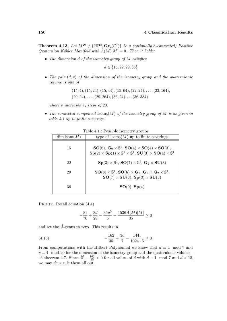
150 4 Classification Results
Theorem 4.13. Let M20 6∈ HP5,Gr2(C7) be a (rationally 3-connected) PositiveQuaternion Kahler Manifold with A(M)[M ] = 0. Then it holds:
• The dimension d of the isometry group of M satisfies
d ∈ 15, 22, 29, 36
• The pair (d, v) of the dimension of the isometry group and the quaternionicvolume is one of
(15, 4), (15, 24), (15, 44), (15, 64), (22, 24), . . . , (22, 164),(29, 24), . . . , (29, 264), (36, 24), . . . (36, 384)
where v increases by steps of 20.
• The connected component Isom0(M) of the isometry group of M is as given intable 4.1 up to finite coverings.
Table 4.1.: Possible isometry groupsdim Isom(M) type of Isom0(M) up to finite coverings
15 SO(6), G2 × S1, SO(4)× SO(4)× SO(3),Sp(2)× Sp(1)× S1 × S1, SU(3)× SO(4)× S1
22 Sp(3)× S1, SO(7)× S1, G2 × SU(3)
29 SO(8)× S1, SO(6)×G2, G2 ×G2 × S1,SO(7)× SU(3), Sp(3)× SU(3)
36 SO(9), Sp(4)
Proof. Recall equation (4.4)
−8170
+3d28− 36u5
5+
1536A(M)[M ]35
≥ 0
and set the A-genus to zero. This results in
−16235
+3d7− 144v
1024 · 5≥ 0(4.13)
From computations with the Hilbert Polynomial we know that d ≡ 1 mod 7 andv ≡ 4 mod 20 for the dimension of the isometry group and the quaternionic volume—cf. theorem 4.7. Since 3d
7 −16235 < 0 for all values of d with d ≡ 1 mod 7 and d < 15,
we may thus rule them all out.
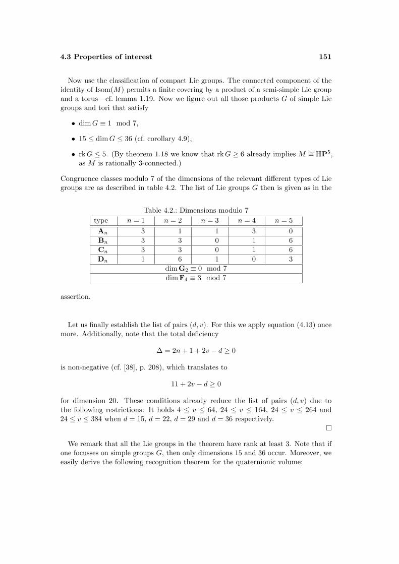
4.3 Properties of interest 151
Now use the classification of compact Lie groups. The connected component of theidentity of Isom(M) permits a finite covering by a product of a semi-simple Lie groupand a torus—cf. lemma 1.19. Now we figure out all those products G of simple Liegroups and tori that satisfy
• dimG ≡ 1 mod 7,
• 15 ≤ dimG ≤ 36 (cf. corollary 4.9),
• rkG ≤ 5. (By theorem 1.18 we know that rkG ≥ 6 already implies M ∼= HP5,as M is rationally 3-connected.)
Congruence classes modulo 7 of the dimensions of the relevant different types of Liegroups are as described in table 4.2. The list of Lie groups G then is given as in the
Table 4.2.: Dimensions modulo 7type n = 1 n = 2 n = 3 n = 4 n = 5An 3 1 1 3 0Bn 3 3 0 1 6Cn 3 3 0 1 6Dn 1 6 1 0 3
dim G2 ≡ 0 mod 7dim F4 ≡ 3 mod 7
assertion.
Let us finally establish the list of pairs (d, v). For this we apply equation (4.13) oncemore. Additionally, note that the total deficiency
∆ = 2n+ 1 + 2v − d ≥ 0
is non-negative (cf. [38], p. 208), which translates to
11 + 2v − d ≥ 0
for dimension 20. These conditions already reduce the list of pairs (d, v) due tothe following restrictions: It holds 4 ≤ v ≤ 64, 24 ≤ v ≤ 164, 24 ≤ v ≤ 264 and24 ≤ v ≤ 384 when d = 15, d = 22, d = 29 and d = 36 respectively.
We remark that all the Lie groups in the theorem have rank at least 3. Note that ifone focusses on simple groups G, then only dimensions 15 and 36 occur. Moreover, weeasily derive the following recognition theorem for the quaternionic volume:
152 4 Classification Results
Corollary 4.14. A 20-dimensional Positive Quaternion Kahler Manifold withA(M)[M ] = 0 and quaternionic volume v > 384 is symmetric.
In chapter D from the appendix we compute the elliptic genus Φ(M) of Wolfspaces. In particular, we see that Φ(M20) = 0 for a 20-dimensional Wolf spaceM 6∼= Gr2(C7). In particular, this implies that A(M)[M ] = A(M,TCM)[M ] = 0,i.e. that i0,0 = i1,1 = 0 in dimension dimM = 20. Equally, this yields sign(M) = 0.This justifies the assumption
A(M)[M ] = A(M,TCM)[M ] = sign(M) = 0
We shall now depict very briefly how this assumption—combined with some more—leads to a classification of Positive Quaternion Kahler Manifolds in dimension 20. Inthis vein we shall see that originally, i.e. mainly before we spotted the mistake inthe classification in dimension 12 (cf. chapter 2), it was possible to prove the mainconjecture 1.6 in dimension 20 under a slight assumption on the Euler characteristic.
The assumption sign(M) = 0 directly yields b2 = b6 = b10 = 0 by Hard-Lefschetz—cf. 1.13. Thus by equation 1.3 the fourth Betti number b4 completely determinesthe Euler characteristic χ(M). By our main linear system of equations we then seethat the index i1,6 is divisible by 5 and that it is restricted to a very small set ofpossible values depending on the dimensions d of the isometry group. Then thecomputations involving the generalised intersection form (cf. theorem 1.16 and lemma4.10) yield that d ∈ 15, 22, 29 requires b4 and thus the Euler characteristic χ(M) tobe relatively large; the smaller is d, the larger is χ(M). Due to table 4.1 we see that indimensions 22 and 29 only isometry groups of rank 4 and 5 appear. The methods wepresent in chapter C of the appendix apply and theorem C.5 and further refinementsof it yield an upper bound for the Euler characteristic. (For this bound to hold weneed to assume that A(M)[M ] = 0 for all 12-dimensional Positive Quaternion KahlerManifolds M with |π2(M)| <∞.) This bound contradicts the values obtained fromthe computations here.
As mentioned above, in the case d = 15 we obtain a large Euler characteristic χ(M)from the computations. So we assume the Euler characteristic to lie below this value;this rules out d = 15 and leaves us with d = 36. As we shall see in theorem 4.22 thiswill suffice—cf. table 4.1—to prove the symmetry of M .
Eventually, we remark that before we encountered the error in the classificationproof for dimension 12—cf. chapter 2—we were able to derive the assumptions onthe A-genus, the twisted A-genus and the signature from the theory. The theoremproposed in [43].2.8 directly ruled out an isometry group of dimension 29, as all thesegroups are of rank 5—cf. table 4.1. However, this theorem is based upon theorem[43].2.6, which lacks a proof—cf. page 21.
4.4 Classification results in dimension 20 153
So it would have been possible to prove the symmetry of 20-dimensional PositiveQuaternion Kahler Manifolds under a slight assumption on the Euler characteristic.
4.4. Classification results in dimension 20
In this section we prove that a Positive Quaternion Kahler Manifold of dimension20 with isometry group one of Sp(4) or SO(9) up to finite coverings is homothetic tothe real Grassmannian Gr4(R9). We shall combine this result with the computationsfrom section 4.3, especially with theorem 4.13. The arguments given in this sectionwill be Lie theoretic mainly.
In this section we obey the following convention: Every statement onequalities, inclusions or decompositions of groups is a statement up tofinite coverings.
First of all note the relation
SO(n)⊗ Sp(1) ∼= (SO(n)× Sp(1))/〈((−1)n+1, (−id)n+1)〉
This can be seen by computing the Lie algebras (cf. [48], p. 25) and determining thefibre of the covering SO(n)× Sp(1)→ SO(n)⊗ Sp(1) over the identity.
From the tables in appendix B in [48], p. 63–68, we cite that all irreducible repre-sentations %(G2) of G2 in degrees smaller than or equal to
• deg % ≤ 30 if % ∈ IrrR(G2)
• deg % ≤ 15 if % ∈ IrrC(G2)
• deg % ≤ 12 if % ∈ IrrH(G2)
are real and have degree
deg % ∈ 7, 14, 27(4.14)
This is considered an exemplary citation of the most important case.We shall use this information in order to shed more light on inclusions of Lie
groups. Some of the following lemmas will be generalised in the next section to higherdimensions. Nonetheless, for the convenience of the reader and since some proofs maybe given in a shorter form, we shall also prove the special cases relevant for dimension20.
Lemma 4.15. Let G = G1 ×G2 be a decomposition of Lie groups. Let further H 6= 1be a simple Lie subgroup of G. Then (up to finite coverings) H is also a subgroup ofone of G1 and G2 (by the canonical projection).
154 4 Classification Results
Proof. Compose the inclusion H → G1 ×G2 with the canonical projection G→ Gi(with i ∈ 1, 2) to obtain a morphism fi : H → Gi. The kernel of fi is a normalsubgroup of H, i.e. we have ker fi ∈ 1, H (up to finite coverings). If ker fi = 1, themorphism fi is an injection and we are done. Otherwise, if ker fi = H, the morphismfi is constant. So if both f1 and f2 are constant, the original inclusion H → G is aconstant map, too. This contradicts H 6= 1.
Lemma 4.16. There is no inclusion of Lie groups SO(7) → Sp(5) (not even up tofinite coverings).
Proof. By table 1.6 the group SO(7) has to be contained in one of
U(5), Sp(4)× Sp(1), Sp(3)× Sp(2), SO(5)⊗ Sp(1)
as there is no quaternionic representation of a simple Lie group H in degree 10 (otherthan the standard representation of Sp(5)) by the tables in appendix B in [48], p. 63–68.(The tables neglect the cases of Lie groups with dimensions smaller than 11. Clearly,so can we.)
Thus, by lemma 4.15 and for dimension reasons, we see that SO(7) has to be asubgroup of one of
SU(5), Sp(4)
Suppose first that SO(7) is a subgroup of SU(5). By table 1.5, lemma 4.15 andfor dimension reasons this is not possible. (Again, there are no further irreduciblecomplex representations of degree 5 of interest.)
Assume SO(7) is a subgroup of Sp(4). We argue in the analogous way to geta contradiction. Alternatively, one may quote table 1.8 for subgroups of maximaldimension.
Lemma 4.17. There is no inclusion of Lie groups SU(5) → SO(9) and equally,SU(5) is not a subgroup of Sp(4) either—not even up to finite coverings.
Proof. Case 1. The group SU(5) cannot be included into SO(9):If this was the case, the group SU(5) would be a maximal rank subgroup of SO(9).
Thus iteratively applying table 1.7 we see that all the subgroups of SO(9) of maximalrank are again products of special orthogonal groups. Indeed, by dimension, we wouldobtain that SU(5) would have to equal SO(8) up to finite coverings; a contradiction.
Case 2. The group SU(5) cannot be included into Sp(4): By table 1.8 a subgroupof maximal dimension of Sp(4) is given by dimension 21 < 24 = dim SU(5).
Lemma 4.18. There is no inclusion of Lie groups Sp(2) × SU(3) → SO(9) andequally, the group Sp(2) × SU(3) also is not a subgroup of Sp(4)—not even up tofinite coverings.
4.4 Classification results in dimension 20 155
Proof. Case 1. The group Sp(2)× SU(3) is not a subgroup of SO(9):Again, we may iteratively use table 1.7 in order to see that all the maximal rank
subgroups of SO(9) are products of special orthogonal groups. Since
rk Sp(2)× SU(3) = 4 = rk SO(9)
this yields the result
Case 2. The group Sp(2)×SU(3) is not a subgroup of Sp(4): Assume the contrary.Since
rk Sp(2)× SU(3) = rk Sp(4) = 4
we derive that Sp(2)× SU(3) necessarily includes into one of
Sp(1)× Sp(3), Sp(2)× Sp(2), U(4)
by means of table 1.7. If it included into Sp(1) × Sp(3), then there would even bean inclusion into Sp(3) (cf. 4.15), which is impossible by rank. If it included intoSp(2)×Sp(2), we would necessarily obtain an inclusion of SU(3) into Sp(2) (cf. 4.15),which is impossible by table 1.8, as a subgroup of Sp(2) of maximal dimension hasdimension 6 < 8 = dim SU(3). An inclusion of Sp(2) × SU(3) into U(4) equallycannot exist by reasons of dimension. This yields a contradiction.
Lemma 4.19. Suppose that k ∈ 3, 4. The only inclusion of Lie groupsSp(k) → Sp(5) is given by the canonical blockwise inclusion up to conjugation.
Proof. Unless Sp(k) is included in the depicted way, it has to be a subgroup of oneof
SU(5), Sp(4)
by lemma 4.15, by table 1.6 and by dimension. (Again, we use that there are nofurther quaternionic representations of degree 10 of interest.)
It cannot be a subgroup of SU(5), as a subgroup of SU(5) of maximal dimensionhas dimension 16 < dim Sp(3) = 21 by table 1.8.
If Sp(3) is a subgroup of Sp(4), then it has to include blockwise (by our usualarguments). As the inclusion of Sp(4) into Sp(5) is also given blockwise, we obtainthe blockwise inclusion of Sp(3) → Sp(5).
Lemma 4.20. There is no inclusion of Lie groups Sp(2) × Sp(2) → Sp(5) unlessone of the Sp(2)-factors includes blockwise (up to conjugation).
156 4 Classification Results
Proof. By table 1.6 and by dimension Sp(2)× Sp(2) includes into one of
U(5), Sp(4)× Sp(1), Sp(3)× Sp(2)
Thus by lemma 4.15 we see that Sp(2)× Sp(2) is a subgroup of one of
SU(5), Sp(3)× Sp(2)
It cannot be a subgroup of SU(5), as a subgroup of SU(5) of maximal dimension is ofdimension 16 < 20 = dim Sp(2)× Sp(2). Thus Sp(2)× Sp(2)⊆Sp(3)× Sp(2) andwe need to determine all the possible inclusions i.
The only inclusion of Sp(2) into Sp(3) possible is given by the canonical blockwiseinclusion (up to conjugation). Suppose now that both Sp(2)-factors do not includeblockwise. We shall lead this to a contradiction.
We obtain that the inclusion composed with the canonical projection
i1 : Sp(2)× 1 → Sp(3)× Sp(2)→ Sp(2)
again is an inclusion. This is due to the fact that the kernel of this map has to betrivial, as Sp(2) is simple. Thus by our assumption of non-blockwise inclusion thekernel has to be the trivial group and i1 is an inclusion. The same holds for
i2 : 1 × Sp(2) → Sp(3)× Sp(2)→ Sp(2)
Without restriction, we may suppose that i1 = i2 = id. Thus we obtain that i is aninclusion if and only if
Sp(2)× Sp(2) → Sp(3)× Sp(2)→ Sp(3)
is an inclusion. By consideration of rank this is impossible. This yields a contradictionand at least one Sp(2)-factor is canonically included.
Lemma 4.21. The only inclusion of Lie groups SU(4) → Sp(5) respectivelySU(4) × Sp(1) → Sp(5) is given by the canonical blockwise inclusion up to con-jugation.
Proof. By table 1.6, by the tables in appendix B in [48], p. 63–68, and by dimensionwe see that SU(4) respectively SU(4)× Sp(1) lies in one of
U(5), Sp(4)× Sp(1), Sp(3)× Sp(2)
The group SU(4) is not a subgroup of Sp(3) by table 1.6 and by dimension. Theonly inclusion of SU(4) into U(5) is given by the canonical blockwise one due to theusual arguments. The group SU(4)× Sp(1) is not a subgroup of U(5); indeed, this isimpossible by table 1.5, the tables in appendix B in [48], p. 63–68, and by dimension.
4.4 Classification results in dimension 20 157
Case 1. Thus in the case of the inclusion SU(4) → Sp(5) we observe that eitherthe inclusion factors over SU(4) → U(4) → Sp(5) and is given blockwise or theinclusion is given via SU(4) → Sp(4) → Sp(5). Again, the inclusion necessarily isgiven blockwise. For this we realise that SU(4) cannot be included into any maximalsubgroup of Sp(4) other than U(4).
Case 2. As for the inclusion SU(4)× Sp(1) → Sp(5) we note that SU(4)× Sp(1)maps into Sp(4)× Sp(1) by dimension. By lemma 4.15 and by dimension we see thatSU(4) again lies in Sp(4). As we have seen this inclusion necessarily is blockwise. AsSp(4) maps into Sp(5) by blockwise inclusion, the inclusion SU(4) → Sp(5) is thecanonical one.
It then remains to see that Sp(1) includes into the Sp(1)-factor of Sp(4)× Sp(1)(and not into the Sp(4)-factor). Assume this is not the case. This means that the groupSp(1) necessarily does include into the Sp(4)-factor. Thus there is a homomorphismof groups
i : SU(4)× Sp(1)→ Sp(4)
with the property that i|SU(4) as well as i|Sp(1) are injective. (Clearly, the morphism iitself cannot be injective.) However, as we shall show, this contradicts the fact that iis a homomorphism: For (x1, x2), (y1, y2) ∈ SU(4)× Sp(1) we compute
i((x1, x2) · (y1, y2)) = i(x1y1, x2y2) = i(x1, 1)i(1, y1)i(1, x2)i(1, y2)i((x1, x2) · (y1, y2)) = i(x1, x2)i(y1, y2) = i(x1, 1)i(1, x2)i(y1, 1)i(1, y2)
Thus we necessarily have that i(1, y1)i(1, x2) = i(1, x2)i(y1, 1). As i|Sp(1) is injective,we realise that—whatever the inclusion i|Sp(1) will be—the group i(Sp(1)) alwayscontains elements that do not commute with every element of SU(4)⊆Sp(4). (Clearly,Sp(1) cannot be included into the centre T 4 of SU(4).)
Consequently, we obtain that the inclusion of Sp(1) into Sp(4)×Sp(1) maps Sp(1)to the Sp(1)-factor and the projection Sp(1)→ Sp(4)× Sp(1)→ Sp(4) is the trivialmap. This proves the assertion.
Let us now prove the classification result.
Theorem 4.22. A 20-dimensional Positive Quaternion Kahler Manifold M whichhas an isometry group Isom(M) that satisfies
Isom0(M) ∈ SO(9),Sp(4)
up to finite coverings is homothetic to the real Grassmannian
M ∼= Gr4(R9)
158 4 Classification Results
Proof. We proceed in three steps. First we shall establish a list of stabiliser groupsin a T 4-fixed-point—where T 4 is the maximal torus of Isom0(M)—that might occurunless M is a Wolf space. As a second step we reduce the list by inclusions into theisometry group and the holonomy group. Finally, in the third step we show by moredistinguished arguments that also the remaining stabilisers from the list cannot occur,whence M has to be symmetric.
Step 1. Both groups SO(9) as well as Sp(4) have rank 4, i.e. they contain a 4-torusT 4 = S1 × · · · × S1. The Positive Quaternion Kahler Manifold M has positive Eulercharacteristic by theorem 1.13. Thus by the Lefschetz fixed-point theorem we derivethat there exists a T 4-fixed-point x ∈ M . Let Hx denote the (identity-componentof the) isotropy group of the G-action in x for G ∈ SO(9),Sp(4). Since G is ofdimension 36 and since dimM = 20, we obtain that dimHx ≥ 17 unless the action ofG on M is transitive. If this is the case, a result by Alekseevskii (cf. [5].14.56, p. 409)yields the symmetry of M . If M is symmetric, it is a Wolf space and the dimension ofthe isometry group then yields that M ∼= Gr4(R9). We may even assume dimHx ≥ 18by the classification of cohomogeneity one Positive Quaternion Kahler Manifolds intheorem [16].7.4, p. 24.
Since rkG = 4 and since x is a T 4-fixed-point, we also obtain rkHx = 4. Moreover,Hx is a closed subgroup. Thus, using lemma 1.19, we may give a list of all products ofsemi-simple Lie groups and tori of dimension 36 ≥ dimHx ≥ 18 and with rkHx = 4up to finite coverings:
SU(5), SO(9), SO(8), Sp(4), Sp(3)× Sp(1), Sp(3)× S1, SO(7)× Sp(1),
SO(7)× S1, SO(6)× Sp(1), Sp(2)× Sp(2), Sp(2)× SU(3), Sp(2)×G2,
G2 ×G2, G2 × SU(3), G2 × Sp(1)× Sp(1), G2 × Sp(1)× S1
Step 2. We now apply two criteria by which we may reduce the list:
• On the one hand we have that Hx is a Lie subgroup of G.
• On the other hand by the isotropy representation Hx is a Lie subgroup ofSp(5)Sp(1)—cf. theorem [45].VI.4.6, p. 248.
We use lemma 4.15 to see that every group Hx in the list contains a factor that has toinclude into Sp(5) up to finite coverings.
An iterative application of table 1.7 yields that every maximal rank subgroup of theclassical group G ∈ SO(9),Sp(4) again is a product of classical groups. Thus Hx
may not be one of the groups
Sp(2)×G2, G2 ×G2, G2 × SU(3), G2 × Sp(1)× Sp(1), G2 × Sp(1)× S1
4.4 Classification results in dimension 20 159
(not even up to finite coverings).Now apply lemma 4.16 in the respective cases to reduce the list of potential stabilisers
to
SU(5), Sp(4), Sp(3)× Sp(1), Sp(3)× S1,
SO(6)× Sp(1), Sp(2)× Sp(2), Sp(2)× SU(3)
Indeed, this lemma rules out all the groups Hx that contain a factor of the form SO(7);and as we see that SO(7) is not a subgroup of Sp(5), also SO(8) and SO(9) cannotbe subgroups of Sp(5).
Now apply lemmas 4.17 and 4.18 by which potential inclusions into the isometrygroup G are made clearer. That is, they rule out the groups SU(5) and Sp(2)×SU(3).Thus the list of possible isotropy groups reduces further to
Sp(4), Sp(3)× Sp(1), Sp(3)× S1, SO(6)× Sp(1), Sp(2)× Sp(2)
Step 3. Let us consider the inclusion of the groups Hx into the holonomy groupSp(5)Sp(1). By 4.15 the largest direct factor of the candidates in our list has tobe a subgroup of Sp(5) (up to finite coverings), as it cannot be included into Sp(1).By lemma 4.19 we see that the inclusion of Sp(4) into Sp(5) and the one of theSp(3)-factor of Sp(3) × Sp(1) respectively of Sp(3) × S1 has to be blockwise. Dueto lemma 4.20 we observe that there is also an Sp(2)-factor of Sp(2) × Sp(2) thatincludes blockwise into Sp(5). Thus we obtain that every group from our list whichcontains a factor of the form Sp(k) for k ≥ 2 has a circle subgroup S1⊆Sp(k) thatincludes into Sp(5) by
diag(S1, 1, 1, 1, 1)⊆diag(Sp(k), 1, . . . , 1)⊆Sp(5)
Thus this circle group fixes a codimension 4 Positive Quaternion Kahler compo-nent. Due to theorem [20].1.2, p. 2, we obtain that M ∼= HP5 or M ∼= Gr2(C7); acontradiction by our assumption on the isometry group.
This leaves us with Hx = SO(6)× SO(3), which is SU(4)× Sp(1) up to (Z2 ⊕ Z2)-covering. Equivalently, we consider an orbit of the form
X : =SO(9)
SO(6)× SO(3)
=Spin(9)
(Spin(6)× Spin(3))/〈(−id,−id)〉
=Spin(9)
(SU(4)× Sp(1))/〈(−id,−1)〉
160 4 Classification Results
Now consider the isotropy representation of the stabiliser group. There are basicallytwo possibilities: Either the whole stabiliser includes into the Sp(5)-factor or theSp(1)-factor includes into the Sp(1)-factor of Sp(5)Sp(1) (and not into the Sp(5)-factor).
In the first case we apply lemma 4.21 to see that the inclusion of SU(4) × Sp(1)into Sp(5) is blockwise. So is the inclusion of the Sp(1)-factor in particular. Thusagain we obtain a sphere which is represented by diag(S1, 1, 1, 1, 1) and which fixes acodimension four quaternionic component. We proceed as above.
Let us now deal with the second case. Again we cite lemma 4.21 to see that theSU(4)-factor includes into Sp(5) in a blockwise way. Observe now that the tangentbundle TM of M splits as
TM = TX ⊕NX
over X, where NX denotes the normal bundle. Since
dimX = dim SO(9)− dim SO(6)× SO(3) = 36− 18 = 18
we obtain that the normal bundle is two-dimensional. Thus the slice representationof the isotropy group (SU(4) × Sp(1))/(−id,−1) at a fixed-point, i.e. the repre-sentation on NX, is necessarily trivial. That is, the action of the isotropy group(SU(4)× Sp(1))/(−id,−1) at a fixed-point has to leave the normal bundle pointwisefixed.
The Sp(1)-factor of SU(4) × Sp(1) maps isomorphically (up to finite coverings)into the Sp(1)-factor of the holonomy group; the SU(4)-factor maps into Sp(5). Thusthe action of this SU(4)× Sp(1) on the tangent space TxM ∼= H5 at x ∈M is givenby (A, h)(v) = Avh−1. This action, however, has no 18-dimensional (respectively2-dimensional) invariant subspace as the Sp(1)-factor acts transitively on each H-component. Hence the normal bundle does not remain fixed under the action of thestabiliser. Thus SU(4)× Sp(1) cannot occur as an isotropy group.
Hence we have excluded all the cases that arose from the assumption dimHx ≥ 18.This was equivalent to the action of the isometry group neither being transitive norof cohomogeneity one. In the latter two cases—as already observed—the manifoldM has to be symmetric. More precisely, since there is no 20-dimensional Wolf spacewith Isom0(M) = Sp(4) (up to finite coverings), we obtain Isom0M = SO(9) andM ∼= Gr4(R9).
We combine this result with previous computations.
Theorem 4.23. A 20-dimensional Positive Quaternion Kahler Manifold M withA(M)[M ] = 0 satisfying
dim Isom0(M) 6∈ 15, 22, 29
4.5 A recognition theorem for the real Grassmannian 161
(where possible groups Isom0(M) in these dimensions can be read off from table 4.1)is a Wolf space.
Proof. This follows by combining theorems 4.13 and 4.22.
Clearly, as for dim Isom0(M) 6∈ 15, 22, 29 one hopes an approach by similartechniques as in the proof of 4.22 to be likewise successful. Yet, we remark that forexample in dimension 29 one will have to cope with five different isometry groups dueto table 4.1. All these groups are of rank 5. So one lists all the possible stabilisers ata T 5-fixed-point on M that do not necessarily make the action of Isom(M) transitiveor of cohomogeneity one. That is, one computes all the products H of semi-simple Liegroups and tori that satisfy rkH = 5 and 11 ≤ dimH ≤ 29. This results in a list of45 possible groups H (up to finite coverings). Following our previous line of argumentwe then try to rule out stabilisers by showing that they either may not include intoa respective isometry group or that they may not be a subgroup of Sp(5)Sp(1). Ifboth is not the case, as a next step we try to show that the way H includes intothe holonomy group already implies the existence of an S1-fixed-point component ofcodomension 4. This would imply the symmetry of the ambient manifold M20. Weobserve that by far the biggest part of this procedure is covered by the argumentswe applied before and we encourage the reader to provide the concrete reasoning.Nonetheless, we encounter new difficulties: For example, the group SU(4)× S1 × S1
includes into the isometry group SU(4) ×G2∼= SO(6) ×G2. If its inclusion into
Sp(5)Sp(1) is induced by the blockwise inclusion of SU(4) into Sp(5), the canonicalinclusion of S1 into Sp(1) and the diagonal inclusion of S1 into Sp(5), we realise thatthere is no codimension four S1-fixed-point component. Then methods more particularin nature will have to be provided—as we did in step 3 of the proof of theorem 4.22.We leave this to the reader.
4.5. A recognition theorem for the real Grassmannian
We shall prove a theorem for Positive Quaternion Kahler Manifolds M4n that recog-nises the isometry type of M by means of the dimension of the isometry group. Thetheorem will determine the isometry type of the manifold when given a large enoughisometry group G. Compare the second point in theorem 1.18, which asserts a recog-nition theorem for the quaternionic projective space and the complex Grassmannian.This result uses the weaker information of the rank of the isometry group. We shalluse it as an important tool. Yet, observe that this theorem is not capable of detectingthe real Grassmannian Gr4(Rn+4); indeed, there seems to be no general recognitiontheorem for Wolf spaces in the literature. (We hint to non-published work by GregorWeingart for a recognition theorem on all indices ip,q—cf. 1.17.) By corollary 1.12we see that both HPn and Gr2(Cn+2) are topologically well-recognisable. Thus a
162 4 Classification Results
main problem with a positive confirmation of conjecture 1.6 lies in identifying thereal Grassmannian and the exceptional Wolf spaces. There seem to be no propertiesknown by which these spaces could be identified.
Since one may relate the index i0,n+2 (cf. 1.17) directly to the dimension ofIsom(M4n), it seems to be pretty natural to try to provide a recognition theorem onthis information. The methods applied extend the ones from section 4.4. Again, weshall neglect finite coverings.
Lemma 4.24. For n ≥ 6 there is no inclusion of Lie groups SO(n + 1) → Sp(n),not even up to finite coverings.
Proof. Due to table 1.6 the group SO(n+ 1) either has to be contained in U(n),Sp(k)×Sp(n− k) with 1 ≤ k ≤ n− 1, some SO(p)⊗Sp(q) with pq = n, p ≥ 3, q ≥ 1or in %(H) for a simple Lie group H and an irreducible quaternionic representation% ∈ IrrH(H) of dimension deg % = 2n. The cases with direct product or tensor productyield an inclusion of SO(n+ 1) in either some SO(k) with k ≥ n—which is impossibleby dimension—or into some smaller symplectic group by lemma 4.15.
Assume there is an inclusion into U(n) = (SU(n)×U(1))/Zn. Then again lemma4.15 yields an inclusion into SU(n). By table 1.5 the maximal subgroups of SU(n)are given by SO(n), Sp(m) with 2m = n, S(U(k)×U(n− k)) for (1 ≤ k ≤ n− 1),SU(p)⊗ SU(q) with pq = n, p ≥ 3, q ≥ 2 and by %(H) for a simple Lie group H andan irreducible quaternionic representation % ∈ IrrC(H) of dimension deg % = n. Aninclusion in the first case is impossible due to dimension. Cases two to four lead toinclusions into smaller symplectic or special unitary groups by lemma 4.15.
Hence we need to have a closer look at irreducible quaternionic and complexrepresentations of simple Lie groups H. The tables in [48], appendix B, p. 63–68,give all the representations of simple Lie groups satisfying a certain dimension bound,which is given by
2 dimH ≥ deg %− 2dimH ≥ deg %− 1
dimH ≥ 32
deg %− 4
for real, complex and quaternionic representations respectively.First of all for n ≥ 3 the tables together with our previous reasoning yield that k = n
is the maximal number for which SU(k) is a maximal subgroup of Sp(n). Equally,for n ≥ 7 we obtain that k = n is the maximal number for which SO(k) is a maximalsubgroup of Sp(n) or of SU(n). This means in particular that SO(n+ 1) cannot beincluded into Sp(n) by a chain
SO(n+ 1)⊆G1⊆ . . . ⊆Gl⊆Sp(n)(4.15)
4.5 A recognition theorem for the real Grassmannian 163
of (irreducible representations of) classical groups G1, . . . , Gl for n ≥ 6.It remains to prove that there is no such chain involving (representations of)
exceptional Lie groups Gi. For this it suffices to realise that there are no exceptionalLie groups H satisfying
dim SO(n+ 1) ≤ dimH ≤ dim Sp(n)(4.16)
with H admitting a quaternionic or complex representation of degree smaller than orequal to 2n or n respectively. (We clearly may neglect the real representations % ofdegree k with k ≤ n, as there evidently cannot be inclusions SO(n+1)⊆ %(H)⊆SO(k)by dimension.)
In table 4.3 for each exceptional Lie group H we give the values of n for whichthe inequalities (4.16) are satisfied. Additionally, we note the corresponding maximaldegree deg % = 2n (deg % = n) of an irreducible quaternionic (complex) representation% by which H might become the subgroup %(H)⊆Sp(k) (%(H)⊆SU(k)) with k ≤ nfor the given values of n. That is, for example in the case of G2 we see that if thereis a quaternionic representation (a complex representation) of degree smaller thanor equal to 22 (to 11), then there is an inclusion of G2 into Sp(k) (into SU(k)) fork ≤ 11 and now also conversely: If there is no such representation, then G2 cannot bea subgroup satisfying SO(n+ 1)⊆G2⊆Sp(n) for any n ∈ N.
Now the tables in [48] yield that there are no quaternionic respectively complex repre-sentations ofH in the degrees depicted in table 4.3. This amounts to the fact that for therelevant values of n from table 4.3 there is no inclusionSO(n + 1)⊆H ⊆Sp(n). Thus by (4.16) there are no inclusions of exceptional Liegroups H with SO(n+ 1)⊆H ⊆Sp(n) for any n ∈ N.
Thus we have proved that there cannot be a chain of the form (4.15) with anexceptional Lie group Gi. Combining this with our previous arguments proves theassertion.
Table 4.3.: Degrees of relevant representationsLie group n ∈ deg % ≤
G2 3, 4 8, 4F4 5, 6, 7, 8, 9 18, 9E6 7, 8, 9, 10, 11 22, 11E7 8, 9, 10, 11, 12, 13, 14, 15 30, 15E8 11, 12, . . . , 20, 21 42, 21
Note that the bound n ≥ 7 in the lemma is necessary since the universal two-sheetedcovering of SO(6) is SU(4). In higher dimensions no such exceptional identities occuras can be seen from the corresponding Dynkin diagrams.
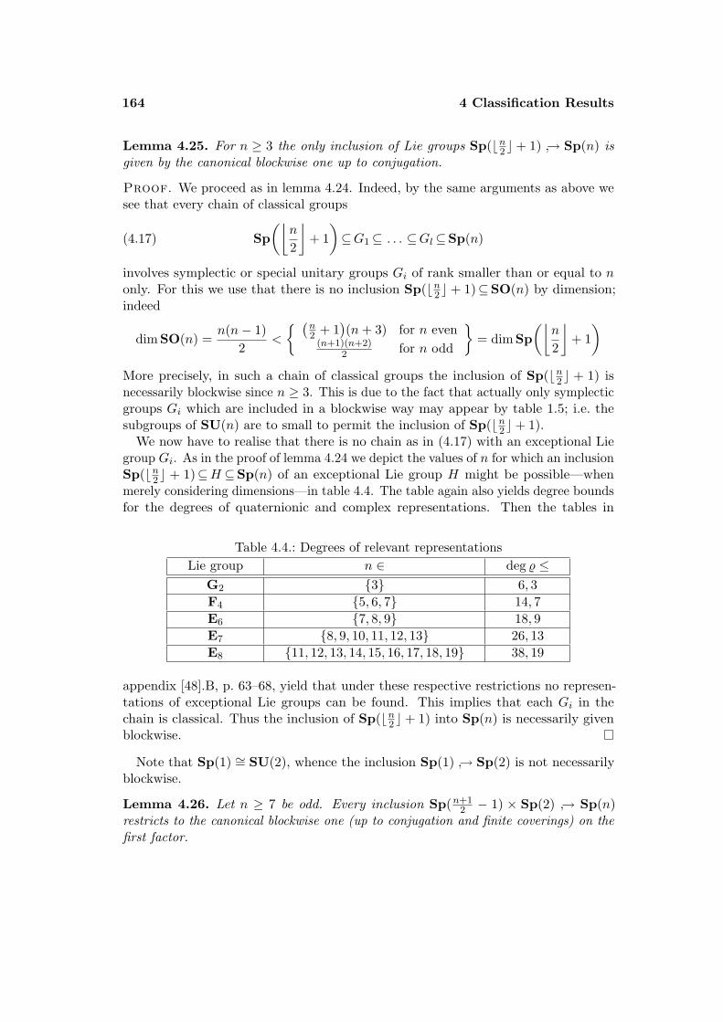
164 4 Classification Results
Lemma 4.25. For n ≥ 3 the only inclusion of Lie groups Sp(bn2 c+ 1) → Sp(n) isgiven by the canonical blockwise one up to conjugation.
Proof. We proceed as in lemma 4.24. Indeed, by the same arguments as above wesee that every chain of classical groups
Sp(⌊
n
2
⌋+ 1)⊆G1⊆ . . . ⊆Gl⊆Sp(n)(4.17)
involves symplectic or special unitary groups Gi of rank smaller than or equal to nonly. For this we use that there is no inclusion Sp(bn2 c+ 1)⊆SO(n) by dimension;indeed
dim SO(n) =n(n− 1)
2<
(n2 + 1
)(n+ 3) for n even
(n+1)(n+2)2 for n odd
= dim Sp
(⌊n
2
⌋+ 1)
More precisely, in such a chain of classical groups the inclusion of Sp(bn2 c + 1) isnecessarily blockwise since n ≥ 3. This is due to the fact that actually only symplecticgroups Gi which are included in a blockwise way may appear by table 1.5; i.e. thesubgroups of SU(n) are to small to permit the inclusion of Sp(bn2 c+ 1).
We now have to realise that there is no chain as in (4.17) with an exceptional Liegroup Gi. As in the proof of lemma 4.24 we depict the values of n for which an inclusionSp(bn2 c + 1)⊆H ⊆Sp(n) of an exceptional Lie group H might be possible—whenmerely considering dimensions—in table 4.4. The table again also yields degree boundsfor the degrees of quaternionic and complex representations. Then the tables in
Table 4.4.: Degrees of relevant representationsLie group n ∈ deg % ≤
G2 3 6, 3F4 5, 6, 7 14, 7E6 7, 8, 9 18, 9E7 8, 9, 10, 11, 12, 13 26, 13E8 11, 12, 13, 14, 15, 16, 17, 18, 19 38, 19
appendix [48].B, p. 63–68, yield that under these respective restrictions no represen-tations of exceptional Lie groups can be found. This implies that each Gi in thechain is classical. Thus the inclusion of Sp(bn2 c+ 1) into Sp(n) is necessarily givenblockwise.
Note that Sp(1) ∼= SU(2), whence the inclusion Sp(1) → Sp(2) is not necessarilyblockwise.
Lemma 4.26. Let n ≥ 7 be odd. Every inclusion Sp(n+12 − 1) × Sp(2) → Sp(n)
restricts to the canonical blockwise one (up to conjugation and finite coverings) on thefirst factor.
4.5 A recognition theorem for the real Grassmannian 165
Proof. By table 1.6 and by dimension we see that Sp(n+12 − 1)×Sp(2) lies in one of
U(n), Sp(k)× Sp(n− k) for 1 ≤ k ≤ n− 1, %(H)
for a simple Lie group H and an irreducible quaternionic representation % of degreedeg % = 2n.
If Sp(n+12 −1)×Sp(2) should happen to appear as a subgroup of SU(n), then table
1.5 would show that
Sp(n+ 1
2− 1)→ SU(n− 1) → SU(n)
necessarily is included in the standard “diagonal” way induced by the standard inclusionH → C2×2. For this we observe the following facts that result when additionally takinginto account the tables in appendix [48].B, p. 63–68: The largest special orthogonalsubgroup (up to finite coverings) of SU(n) is SO(n) for n ≥ 6. The group SO(n) doesnot permit Sp(n+1
2 − 1) as a subgroup for n ≥ 4. Moreover, there are no irreduciblecomplex representations by which a simple Lie group H might include into some SU(k)(for k ≤ n) satisfying Sp(n+1
2 − 1)⊆H.Now we see that whenever Sp(n+1
2 −1) is included diagonally into SU(n) as depicted,there is no inclusion of Sp(n+1
2 − 1) × Sp(2) possible. That is, for the inclusion ofthis direct product to be a homomorphism we need the group Sp(2) to map into thecentraliser CSU(n)(Sp(n+1
2 − 1)) of Sp(n+12 − 1) in SU(n). Yet, we obtain
CSU(n)
(Sp(n+ 1
2− 1))∼= S1 × S1
and thus no inclusion of Sp(2) is possible. Hence Sp(n+12 − 1)× Sp(2) cannot be a
subgroup of U(n).
The tables in [48] again yield that whenever a simple Lie group H is included intoSp(k) (for k ≤ n) via an irreducible quaternionic representation %, the inclusion is oneof
SU(6) → Sp(10), SO(11) → Sp(16), SO(12) → Sp(16), E7 → Sp(28)
or an inclusion of a symplectic group of rank smaller than k unless the degree ofthe representation is far too large to be of interest for our purposes. Indeed, alreadythe depicted inclusions are not relevant, since Sp(n+1
2 − 1) cannot be included intoSU(6), SO(11), SO(12), E7 respectively when n ≥ 10, 16, 16, 28.
Thus we see that every inclusion of Sp(n+12 − 1)× Sp(2) has to factor through one
of Sp(n− k)× Sp(k) for 1 ≤ k ≤ n− 1. Hence for 1 ≤ k < n+12 − 1 we obtain that
166 4 Classification Results
the only inclusion of Sp(n+12 − 1) into Sp(n) factoring through Sp(n− k)× Sp(k) is
given by standard blockwise inclusion
Sp(n+ 1
2− 1)→ Sp(n− k) → Sp(k)
Thus we may assume without restriction that k = n+12 − 1 (and n − k = n+1
2 ) andthat the inclusion of Sp(n+1
2 − 1) → Sp(n) is not the standard blockwise one. Thuswe see that the inclusion necessarily factors over
Sp(n+ 1
2− 1)→ Sp
(n+ 1
2− 1)× Sp
(n+ 1
2
)→ Sp(n)
where the first inclusion splits as a product of the standard blockwise inclusions
Sp(n+ 1
2− 1)
id→ Sp
(n+ 1
2− 1)
Sp(n+ 1
2− 1)→ Sp
(n+ 1
2
)So regard Sp(n+1
2 − 1) as the subgroup of Sp(n) given by this inclusion. Again wemake use of the fact that the Sp(2)-factor has to include into the centraliser
CSp(n)
(Sp(n+ 1
2− 1))∼= S1 × S1 × Sp(1)
Such an inclusion clearly is impossible and we obtain a contradiction. Thus theinclusion of Sp(n+1
2 − 1)× Sp(2) is the standard blockwise one when restricted to theSp(n+1
2 − 1)-factor.
Lemma 4.27. In table 4.5 the semi-simple Lie groups of maximal dimension withrespect to a fixed rank (from rank 1 to rank 12) are given up to isomorphisms andfinite coverings. From rank 13 on the groups that are maximal in this sense are givenby the two infinite series Sp(n) and SO(2n+ 1) only.
Proof. Table 4.5 results from a case by case check using table 1.3. From dimension13 on semi-simple Lie groups involving factors that are exceptional Lie groups aresmaller than the largest classical groups. Among products of classical groups the ratiobetween dimension and rank is maximal for the types Bn and Cn,
Let us now prove the classification theorem that actually may be regarded as arecognition theorem for the real Grassmannian.
Theorem 4.28. Let M4n be a Positive Quaternion Kahler Manifold. Suppose thatthe dimension of the isometry group dim Isom(M4n) satisfies the respective condition
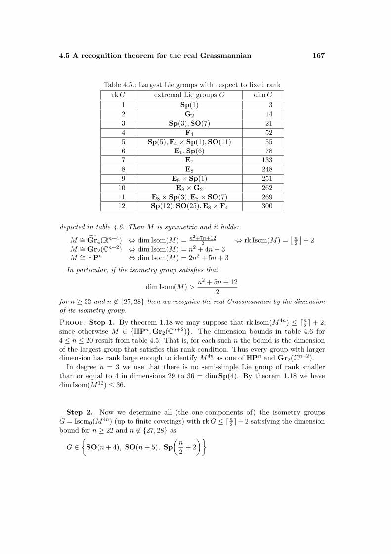
4.5 A recognition theorem for the real Grassmannian 167
Table 4.5.: Largest Lie groups with respect to fixed rankrkG extremal Lie groups G dimG
1 Sp(1) 32 G2 143 Sp(3),SO(7) 214 F4 525 Sp(5),F4 × Sp(1),SO(11) 556 E6,Sp(6) 787 E7 1338 E8 2489 E8 × Sp(1) 251
10 E8 ×G2 26211 E8 × Sp(3),E8 × SO(7) 26912 Sp(12),SO(25),E8 × F4 300
depicted in table 4.6. Then M is symmetric and it holds:
M ∼= Gr4(Rn+4) ⇔ dim Isom(M) = n2+7n+122 ⇔ rk Isom(M) =
⌊n2
⌋+ 2
M ∼= Gr2(Cn+2) ⇔ dim Isom(M) = n2 + 4n+ 3M ∼= HPn ⇔ dim Isom(M) = 2n2 + 5n+ 3
In particular, if the isometry group satisfies that
dim Isom(M) >n2 + 5n+ 12
2for n ≥ 22 and n 6∈ 27, 28 then we recognise the real Grassmannian by the dimensionof its isometry group.
Proof. Step 1. By theorem 1.18 we may suppose that rk Isom(M4n) ≤ dn2 e + 2,since otherwise M ∈ HPn,Gr2(Cn+2). The dimension bounds in table 4.6 for4 ≤ n ≤ 20 result from table 4.5: That is, for each such n the bound is the dimensionof the largest group that satisfies this rank condition. Thus every group with largerdimension has rank large enough to identify M4n as one of HPn and Gr2(Cn+2).
In degree n = 3 we use that there is no semi-simple Lie group of rank smallerthan or equal to 4 in dimensions 29 to 36 = dim Sp(4). By theorem 1.18 we havedim Isom(M12) ≤ 36.
Step 2. Now we determine all (the one-components of) the isometry groupsG = Isom0(M4n) (up to finite coverings) with rkG ≤ dn2 e+ 2 satisfying the dimensionbound for n ≥ 22 and n 6∈ 27, 28 as
G ∈
SO(n+ 4), SO(n+ 5), Sp(n
2+ 2)
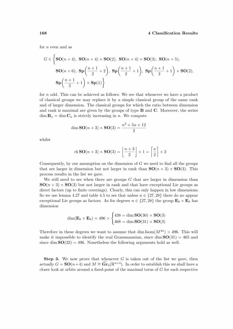
168 4 Classification Results
for n even and as
G ∈
SO(n+ 4), SO(n+ 4)× SO(2), SO(n+ 4)× SO(3), SO(n+ 5),
SO(n+ 6), Sp(n+ 1
2+ 2), Sp
(n+ 1
2+ 1), Sp
(n+ 1
2+ 1)× SO(2),
Sp(n+ 1
2+ 1)× Sp(1)
for n odd. This can be achieved as follows: We see that whenever we have a productof classical groups we may replace it by a simple classical group of the same rankand of larger dimension. The classical groups for which the ratio between dimensionand rank is maximal are given by the groups of type B and C. Moreover, the seriesdim Bn = dim Cn is strictly increasing in n. We compute
dim SO(n+ 3)× SO(3) =n2 + 5n+ 12
2
whilst
rk SO(n+ 3)× SO(3) =⌊n+ 3
2
⌋+ 1 =
⌈n
2
⌉+ 2
Consequently, by our assumption on the dimension of G we need to find all the groupsthat are larger in dimension but not larger in rank than SO(n + 3) × SO(3). Thisprocess results in the list we gave.
We still need to see when there are groups G that are larger in dimension thanSO(n+ 3)× SO(3) but not larger in rank and that have exceptional Lie groups asdirect factors (up to finite coverings). Clearly, this can only happen in low dimensions.So we use lemma 4.27 and table 4.5 to see that unless n ∈ 27, 28 there do no appearexceptional Lie groups as factors. As for degrees n ∈ 27, 28 the group E8 ×E8 hasdimension
dim(E8 ×E8) = 496 >
438 = dim SO(30)× SO(3)468 = dim SO(31)× SO(3)
Therefore in these degrees we want to assume that dim Isom(M4n) > 496. This willmake it impossible to identify the real Grassmannian, since dim SO(31) = 465 andsince dim SO(32) = 496. Nonetheless the following arguments hold as well.
Step 3. We now prove that whenever G is taken out of the list we gave, thenactually G = SO(n+4) and M ∼= Gr4(Rn+4). In order to establish this we shall have acloser look at orbits around a fixed-point of the maximal torus of G for each respective
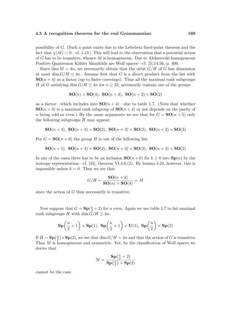
4.5 A recognition theorem for the real Grassmannian 169
possibility of G. (Such a point exists due to the Lefschetz fixed-point theorem and thefact that χ(M) > 0—cf. 1.13.) This will lead to the observation that a potential actionof G has to be transitive, whence M is homogeneous. Due to Alekseevski homogeneousPositive Quaternion Kahler Manifolds are Wolf spaces—cf. [5].14.56, p. 409.
Since dimM = 4n, we necessarily obtain that the orbit G/H of G has dimensionat most dimG/H ≤ 4n. Assume first that G is a direct product from the list withSO(n+ 4) as a factor (up to finite coverings). Thus all the maximal rank subgroupsH of G satisfying dimG/H ≤ 4n for n ≥ 22, necessarily contain one of the groups
SO(n)× SO(4), SO(n+ 3), SO(n+ 2)× SO(2)
as a factor—which includes into SO(n + 4)—due to table 1.7. (Note that whetherSO(n+ 3) is a maximal rank subgroup of SO(n+ 4) or not depends on the parity ofn being odd or even.) By the same arguments we see that for G = SO(n+ 5) onlythe following subgroups H may appear:
SO(n+ 4), SO(n+ 3)× SO(2), SO(n+ 2)× SO(2), SO(n+ 2)× SO(3)
For G = SO(n+ 6) the group H is out of the following list:
SO(n+ 5), SO(n+ 4)× SO(2), SO(n+ 3)× SO(3), SO(n+ 3)× SO(2)
In any of the cases there has to be an inclusion SO(n+ k) for k ≥ 0 into Sp(n) by theisotropy representation—cf. [45], theorem VI.4.6.(2). By lemma 4.24, however, this isimpossible unless k = 0. Thus we see that
G/H =SO(n+ 4)
SO(n)× SO(4)= M
since the action of G thus necessarily is transitive.
Now suppose that G = Sp(n2 + 2) for n even. Again we use table 1.7 to list maximalrank subgroups H with dimG/H ≤ 4n:
Sp(n
2+ 1)× Sp(1), Sp
(n
2+ 1)×U(1), Sp
(n
2
)× Sp(2)
If H = Sp(n2 )×Sp(2), we see that dimG/H = 4n and that the action of G is transitive.Thus M is homogeneous and symmetric. Yet, by the classification of Wolf spaces wederive that
M =Sp(n2 + 2
)Sp(n2
)× Sp(2)
cannot be the case.
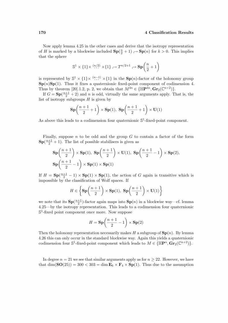
170 4 Classification Results
Now apply lemma 4.25 in the other cases and derive that the isotropy representationof H is marked by a blockwise included Sp(n2 + 1) → Sp(n) for k > 0. This impliesthat the sphere
S1 × 1× (n/2). . . ×1 → Tn/2+1 → Sp(n
2+ 1)
is represented by S1 × 1× (n−1). . . ×1 in the Sp(n)-factor of the holonomy groupSp(n)Sp(1). Thus it fixes a quaternionic fixed-point component of codimension 4.Thus by theorem [20].1.2, p. 2, we obtain that M4n ∈ HP4n,Gr2(Cn+2).
If G = Sp(n+12 + 2) and n is odd, virtually the same arguments apply. That is, the
list of isotropy subgroups H is given by
Sp(n+ 1
2+ 1)× Sp(1), Sp
(n+ 1
2+ 1)×U(1)
As above this leads to a codimension four quaternionic S1-fixed-point component.
Finally, suppose n to be odd and the group G to contain a factor of the formSp(n+1
2 + 1). The list of possible stabilisers is given as
Sp(n+ 1
2
)× Sp(1), Sp
(n+ 1
2
)×U(1), Sp
(n+ 1
2− 1)× Sp(2),
Sp(n+ 1
2− 1)× Sp(1)× Sp(1)
If H = Sp(n+12 − 1) × Sp(1) × Sp(1), the action of G again is transitive which is
impossible by the classification of Wolf spaces. If
H ∈
Sp(n+ 1
2
)× Sp(1), Sp
(n+ 1
2
)×U(1)
we note that its Sp(n+1
2 )-factor again maps into Sp(n) in a blockwise way—cf. lemma4.25—by the isotropy representation. This leads to a codimension four quaternionicS1-fixed point component once more. Now suppose
H = Sp(n+ 1
2− 1)× Sp(2)
Then the holonomy representation necessarily makes H a subgroup of Sp(n). By lemma4.26 this can only occur in the standard blockwise way. Again this yields a quaternioniccodimension four S1-fixed-point component which leads to M ∈ HPn,Gr2(Cn+2).
In degree n = 21 we see that similar arguments apply as for n ≥ 22. However, we havethat dim(SO(25)) = 300 < 303 = dim E6 × F4 × Sp(1). Thus due to the assumption
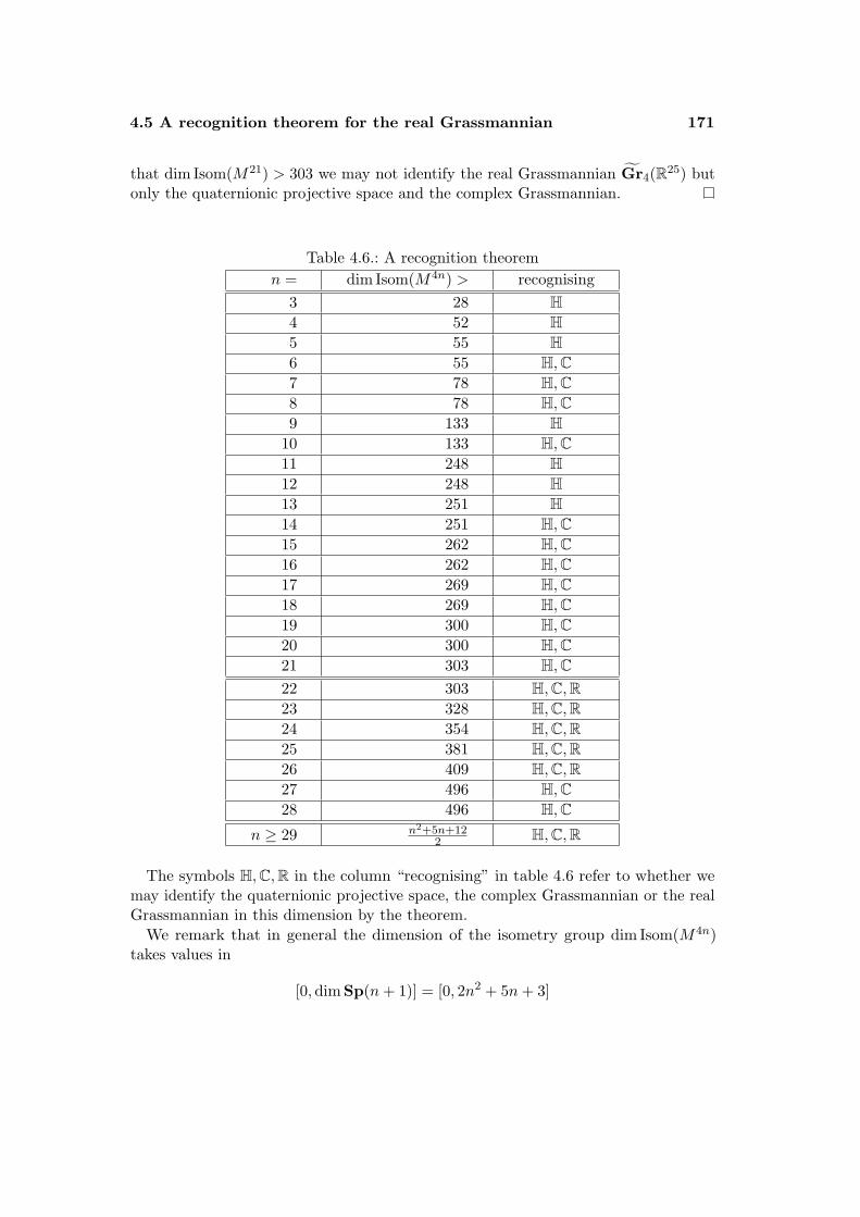
4.5 A recognition theorem for the real Grassmannian 171
that dim Isom(M21) > 303 we may not identify the real Grassmannian Gr4(R25) butonly the quaternionic projective space and the complex Grassmannian.
Table 4.6.: A recognition theoremn = dim Isom(M4n) > recognising
3 28 H4 52 H5 55 H6 55 H,C7 78 H,C8 78 H,C9 133 H
10 133 H,C11 248 H12 248 H13 251 H14 251 H,C15 262 H,C16 262 H,C17 269 H,C18 269 H,C19 300 H,C20 300 H,C21 303 H,C22 303 H,C,R23 328 H,C,R24 354 H,C,R25 381 H,C,R26 409 H,C,R27 496 H,C28 496 H,C
n ≥ 29 n2+5n+122 H,C,R
The symbols H,C,R in the column “recognising” in table 4.6 refer to whether wemay identify the quaternionic projective space, the complex Grassmannian or the realGrassmannian in this dimension by the theorem.
We remark that in general the dimension of the isometry group dim Isom(M4n)takes values in
[0, dim Sp(n+ 1)] = [0, 2n2 + 5n+ 3]
172 4 Classification Results
(cf. 1.18). Hence—apart from recognising the real Grassmannian—this theorems rulesout approximately three quarters of all possible values. For example when taking intoaccount more structure data for exceptional Lie groups one certainly may generalisethe theorem with ease.
This theorem now shows that the whole question whether Positive QuaternionKahler Manifolds M4n are symmetric or not boils down to a computation of thedimension of the isometry group Isom(M4n).
A Positive Quaternion Kahler Manifold M4n is symmetric (for almostevery n) if and only if dim Isom(M) > n2+5n+12
2 .
Furthermore, by theorem 1.17 one may interpret the dimension of the isometrygroup as the index of a twisted Dirac operator, i.e. i0,n+2 = dim Isom(M). As amajor consequence of a non-published formula by Gregor Weingart one obtains thata Positive Quaternion Kahler Manifold is a Wolf space if and only if all the indicesip,q and Betti numbers coincide with the ones of the symmetric example. As we haveproved by our approach—which is certainly much simpler than the highly elaboratedtechniques applied by Gregor Weingart—the index i0,n+2 already suffices for such aconclusion in almost every dimension. This lets us extend our statement from above:
The question whether a Positive Quaternion Kahler Manifold M4n issymmetric or not can (almost always) be decided from the index
ind(D/(Sn+2H)) = 〈A(M) · ch(Sn+2H), [M ]〉
(For the bundle H and the indices ip,q we refer to the notation from the introduction,section 1.1.)
A
Cohomology of Wolf Spaces
Although the results are well-known, for the convenience of the reader we shall computethe rational cohomology of the three infinite series of Wolf spaces up to degree 8.Recall that the series are given by the quaternionic projective space, the complexGrassmannian and the oriented real Grassmannian:
HPn =Sp(n+ 1)
Sp(n)× Sp(1)(A.1)
Gr2(Cn+2) =U(n+ 2)
U(n)×U(2)(A.2)
Gr4(Rn+4) =SO(n+ 4)
SO(n)× SO(4)(A.3)
The computation of the cohomology of HPn will illustrate the method.We refer to the “stable case” as to the cohomology of Gr2(C∞) and of Gr4(R∞)
respectively.
Theorem A.1. For the quaternionic projective space it holds:
H∗(HPn,Q) = Q[u]/un+1
Iff n ≥ 4 we are in the stable case and obtain
H i(Gr2(Cn+2)) =
0 for i oddQ for i = 0〈l〉Q for i = 2〈l2, x〉Q for i = 4〈l3, lx〉Q for i = 6〈l4, l2x, x2〉Q for i = 8
174 A Cohomology of Wolf Spaces
For the complex Grassmannian we have: If n is odd and iff n ≥ 5 we are in the stablecase and obtain
H i(Gr4(Rn+4)) =
0 for i ∈ 2, 6 or i oddQ for i = 0〈u, x〉Q for i = 4〈u2, ux, x2〉Q for i = 8
For the real Grassmannian we obtain: If n is even and iff n ≥ 10 we are in the stablecase and obtain
H i(Gr4(Rn+4)) =
0 for i ∈ 2, 6 or i oddQ for i = 0〈l2, x〉Q for i = 4〈l4, l2x, x2〉Q for i = 8
In lower dimensions we have the following cohomology algebras:
H∗(Gr2(C3)) = Q[l]/l3 deg l = 2
H∗(Gr2(C4)) = Q[l, x]/lx = 0, x2 = l4 deg l = 2, deg x = 4
H∗(Gr2(C5)) = Q[l, x]/R3 deg l = 2, deg x = 4
H∗(Gr2(C6)) = Q[l, x]/R4 deg l = 2, deg x = 4
H∗(Gr2(C7)) = Q[l, x]/R5 deg l = 2, deg x = 4
H∗(Gr4(R5)) = Q[u]/u2 deg u = 4
H∗(Gr4(R6)) = Q[l, x]/l3 = 2lx, x2 = l2x deg l = 2,deg x = 4
H∗(Gr4(R7)) = Q[l, x]/R1 deg l = deg x = 4
H∗(Gr4(R8)) = Q[l, x, y]/R2,R′2 deg l = deg x = deg y = 4
H∗(Gr4(R9)) = Q[l, x]/R2 deg l = deg x = 4
In order to complete the list of low-dimensional Wolf spaces we compute
H∗(G2/SO(4)) = Q[u]/u3 deg u = 4
The relations Rn consist of setting σi = 0 for i > n in the following list and the
A Cohomology of Wolf Spaces 175
relations R′i require σi = y2.
σ1 = −lσ2 = l2 − xσ3 = 2lx− l3
σ4 = l4 − 3l2x+ x2
σ5 = −l5 + 4l3x− 3lx2
σ6 = l6 − 5l4x+ 6l2x2 − x3
σ7 = −l7 + 6l5x− 10l3x2 + 4lx3
σ8 = l8 − 7l6x+ 15l4x2 − 10l2x3 + x4
σ9 = l9 + 8l7x− 21l5x2 + 20l3x3 − 5lx4
σ10 = l10 − 9l8x+ 28l6x2 − 35l4x3 + 15l2x4 − x5
This yields the following cohomology groups with relations (without linear dependenciesbetween generators).
H i(Gr2(C4)) =
〈σ1〉Q for i = 2〈σ2
1, σ2〉Q for i = 4〈σ3
1〉Q for i = 6〈σ4
1〉Q for i = 8
σ1σ2 = σ31/2, σ
22 = σ4
1/2
H i(Gr2(C5)) =
〈σ1〉Q for i = 2〈σ2
1, σ2〉Q for i = 4〈σ3
1, σ1σ2〉Q for i = 6〈σ4
1, σ21σ2〉Q for i = 8
σ22 = −σ4
1 + 3σ21σ2
H i(Gr4(R6)) =
〈σ′1〉Q for i = 2〈σ′21 , σ′2〉Q for i = 4〈σ′31 〉Q for i = 6〈σ′41 〉Q for i = 8
σ′1σ′2 = 0, (σ′2)2 = (σ′1)4
H i(Gr4(R7)) =
〈σ1, σ
′2〉Q for i = 4
〈(σ1)2, σ1σ′2〉Q for i = 8
(σ′2)2 = (σ1)2
H i(Gr4(R8)) =
〈σ′2, σ1, σ
′2〉Q for i = 4
〈(σ1)2, σ1σ′2, σ1σ
′2, σ
22〉Q for i = 8
(σ′2)2 = σ21 − (σ′2)2, σ′2σ
′2 = 0
Observe that these results reflect the ring structure in low degrees and the well-knownisometries Gr2(C3) ∼= CP2, Gr4(R5) ∼= HP1 ∼= S4, Gr4(R6) ∼= Gr2(C4).
176 A Cohomology of Wolf Spaces
Proof. It holds
H∗(HPn) = H∗(B(Sp(n)× Sp(1))/H>0(BSp(n+ 1))
= H∗(BT )W(Sp(n)×Sp(1))/H>0(BT )W(Sp(n+1))(A.4)
where T denotes the maximal torus of Sp(n + 1) and W is the Weyl group. Nowrecall that the Weyl group of Sp(n) is given by G(n), the group of permutations φ ofthe set −n, . . . ,−1, 1, . . . , n satisfying φ(−v) = −φ(v) (cf. [11], p. 171). The groupacts on the maximal torus by φ−1(θ1, . . . , θn) = (θφ(1), . . . , θφ(n)), where the θi denotethe angles of the corresponding rotations. By convention we write θ−v = −θv. Recallthat the cohomology of the classifying space BT is the polynomial algebra on n+ 1generators xi in degree 2 corresponding to the θi. Due to these remarks it becomesobvious that the cohomology of HPn is generated by those polynomials symmetric inx1, . . . , xn which are invariant under xi 7→ −xi for all 1 ≤ i ≤ n respectively by thepolynomials in xn+1 which are invariant under xn+1 7→ −xn+1. These are exactly theelementary symmetric polynomials σ1, . . . , σn in the x2
i for 1 ≤ i ≤ n and σ1 = x2n+1.
So (A.4) equals
Q[σ1, . . . σn, σ1]/σσ = 1=Q[σ1, . . . σn, σ1])/σ1 = −σ1, σ2 = σ2
1, . . . , σn = (−1)nσn1 , σn+11 = 0
=Q[σ1]/σn+11
where σ = 1 + σ1 + . . . σn respectively σ = 1 + σ1. (Recall that the elementarysymmetric polynomials in x1, . . . , xn+1 can be described as σσ.)
Now let us compute the cohomology of the complex Grassmannian. As above weobtain
H∗(Gr2(Cn+2)) = H∗(BT )W(U(n)×U(2))/H>0(BT )W(U(n+2))
= Q[σ1, . . . , σn, σ1, σ2]/σσ = 1
where the σi are the elementary symmetric polynomials in the xi for 1 ≤ i ≤ n andthe σi are the elementary symmetric polynomials in xn+1, xn+2. (Recall that the Weylgroup of U(n) is just the symmetric group Sn.) From the relation σσ = 1 we compute
A Cohomology of Wolf Spaces 177
in each degree:
σ1 = −σ1
σ2 = σ21 − σ2
σ3 = 2σ1σ2 − σ31
σ4 = σ41 − 3σ2
1σ2 + σ22
σ5 = −σ51 + 4σ3
1σ2 − 3σ1σ22
σ6 = σ61 − 5σ4
1σ2 + 6σ21σ
22 − σ3
2
σ7 = −σ71 + 6σ5
1σ2 − 10σ31σ
22 + 4σ1σ
32
σ8 = σ81 − 7σ6
1σ2 + 15σ41σ
22 − 10σ2
1σ32 + σ4
2
σ9 = σ91 + 8σ7
1σ2 − 21σ51σ
22 + 20σ3
1σ32 − 5σ1σ
42
σ10 = σ101 − 9σ8
1σ2 + 28σ61σ
22 − 35σ4
1σ32 + 15σ2
1σ42 − σ5
2
(A.5)
This yields the first cohomology groups
H2(Gr2(Cn+2)) = 〈σ1〉QH4(Gr2(Cn+2)) = 〈σ2
1, σ2〉QH6(Gr2(Cn+2)) = 〈σ3
1, σ1σ2〉QH8(Gr2(Cn+2)) = 〈σ4
1, σ21σ2, σ
22〉Q
for n ≥ 4 (without any linear relations between the generators). In low dimensions weobtain additional restrictions by setting the corresponding equations in (A.5) to zero,i.e. σi = 0 for i > n.
The same procedure for the real Grassmannian yields the following: The Weyl groupof SO(n) for odd n is G(n). For even n it is SG(n) consisting of even permutations ofG(n). So in the odd case invariant polynomials again are generated by elementarysymmetric polynomials in the xi. In the even case the n-th elementary symmetricpolynomial in the x2
i can be replaced by the n-th elementary symmetric polynomialσ′n = x1 · x2 · · ·xn. (A permuation is in SG(n) iff it causes a change of sign on an evennumber of xi. Thus it has no effect on σ′n.) In the case that n is odd we obtain
H∗(Gr4(Rn+4)) = H∗(BT )W(SO(n)×SO(4))/H>0(BT )W(SO(n+4))
= Q[σ1, . . . , σ(n−1)/2, σ1, σ′2]/σσ = 1
where the σi are the elementary symmetric polynomials in the x2i for
1 ≤ i ≤ (n−1)/2, the σi are the elementary symmetric polynomials in x2(n+1)/2, x
2(n+3)/2
and σ′2 = x(n+1)/2 · x(n+3)/2 with (σ′2)2 = σ2. So we obtain the relations (A.5) in our
178 A Cohomology of Wolf Spaces
terminology. For n ≥ 5 this yields the following cohomology groups (without anylinear relations between generators).
H4(Gr4(Rn+4)) = 〈σ1, σ′2〉Q
H8(Gr4(Rn+4)) = 〈σ21, σ1σ
′2, σ2〉Q
In low dimensions we obtain cohomology algebras as in the assertion by setting thecorresponding σi to zero.
If n is even we have
H∗(Gr4(Rn+4)) = H∗(BT )W(SO(n)×SO(4))/H>0(BT )W(SO(n+4))
= Q[σ1, . . . , σ(n−2)/2, σ′n/2, σ1, σ
′2]/σσ = 1, σ′n/2σ
′2 = 0
where σ′n/2 = x1 · · ·xn/2. Using the relations (A.5) we obtain for n ≥ 10 that
H4(Gr4(Rn+4)) = 〈σ1, σ′2〉Q
H8(Gr4(Rn+4)) = 〈σ21, σ1σ
′2, σ2〉Q
and, as usual, the cohomology groups in degrees 1 to 3 and 5 to 7 vanish. A computationof the relations in the particular cases yields the corresponding results.
The ring structure of G2/SO(4) can be derived in the same way: The Weyl groupof G2 is the symmetry group of the regular hexagon, i.e. the dihedral group D6. Themaximal torus of G2 can be regarded as the quotient of the full hexagon by identifyingopposite sides and collapsing one such pair. Thus the Weyl group acts on T as asymmetry group, i.e. given generating loops x, y and
D6 = Z6 o Z2 = 〈d, s | d6 = 1, s2 = 1, dsd = d−1〉
we obtain the relations:
dx = y, d2x = y − x, d3x = −x, d4x = −y, d5x = x− y, d6x = x, sx = y, s2x = x
A polynomial in x and y invariant under D6 must be symmetric due to the action ofs, so again it must be generated by the elementary symmetric polynomials σ′1 andσ′2 in x and y. Now a simple calculation using the invariance under the action of dshows that the polynomial (σ′1)2 − 3σ′2 is (up to multiples) the only polynomial indegree 4 invariant under the action of D6. In degree 8 no such polynomial exists.Set σ1 = x2 + y2 (the first elementary symmetric polynomial in x2, y2) and obtain(σ′1)2 − 3σ′2 = σ1 − σ′2. So the following computations yield the desired result:
H∗(G2/SO(4)) = H∗(BT )W(SO(4))/H>0(BT )W(G2)
A Cohomology of Wolf Spaces 179
Set u = σ1. The relation σ1 = σ′2 yields H4(G2/SO(4)) = 〈u〉Q. The non-existence ofrelations in degree eight yields H8(G2/SO(4)) = 〈u2〉Q.
Observe that the isomorphism H∗(Gr2(C4)) ∼= H∗(Gr4(R6)) is given by l 7→ l andx 7→ l2 + 2x.
As a corollary we obtain the Betti numbers in low dimensions.
Corollary A.2. Betti numbers are concentrated in degrees divisible by two for thecomplex Grassmannian, in degrees divisible by four for the other Wolf spaces—exceptfor Gr2(C4) ∼= Gr4(R6). Non-trivial Betti numbers bi are given (mostly) up to duality.The Euler characteristic χ is computed.
HPn : b0 = b4 = · · · = bn = 1, χ = n+ 1
Gr2(C3) : b0 = 1, b2 = 1 χ = 3
Gr2(C4) : b0 = 1, b2 = 1, b4 = 2 χ = 6
Gr2(C5) : b0 = 1, b2 = 1, b4 = 2, b6 = 2 χ = 10
Gr2(C6) : b0 = 1, b2 = 1, b4 = 2, b6 = 2, b8 = 3 χ = 15
Gr2(C7) : b0 = 1, b2 = 1, b4 = 2, b6 = 2, b8 = 3, b10 = 3 χ = 21
Gr4(R5) : b0 = 1, b4 = 1 χ = 2
Gr4(R6) : b0 = 1, b2 = 1, b4 = 2 χ = 6
Gr4(R7) : b0 = 1, b4 = 2 χ = 6
Gr4(R8) : b0 = 1, b4 = 3, b8 = 4 χ = 12
Gr4(R9) : b0 = 1, b4 = 2, b8 = 3 χ = 12
G2/SO(4) : b0 = b4 = b8 = 1 χ = 3

B
Isometric Group Actions onWolf Spaces
In this chapter we shall describe the fixed-point components of isometric circle-actionsand certain isometric involutions on the infinite series of Wolf-spaces.
B.1. Isometric circle actions
Let us classify isometric circle actions together with their fixed-point components onthe three infinite series. Observe that each element of the isometry group may be takento lie in a maximal torus and any two maximal tori are conjugated. Since a one-sphereadmits a topological generator, we may thus consider the sphere to be part of themaximal torus. Equally, this does not impose any restriction on the structure of possiblefixed-point components, since conjugation satisfies tst−1(t(x)) = t(x)⇔ s(x) = x (forany two isometries s and t acting on M 3 x). We have
rk Isom(HPn) = n+ 1
rk Isom(Gr2(Cn+2)) = n+ 1
rk Isom(Gr4(Rn+4)) =⌊n+ 4
2
⌋(Note that we have to write Gr2(Cn+2) = SU(n+ 2)/(S(U(n)×U(2))) in order toreveal a group acting almost effectively.)
We shall bear in mind the following line of argument: The description of a Grass-mannian as a homogeneous space may be interpreted as follows. The isometry groupacts transitively on the manifold. So every plane can be obtained by multiplyinga basis of a standard coordinate plane in the ambient vector space with a suitable
182 B Isometric Group Actions on Wolf Spaces
element of the isometry group and eventually by forming the quotient with all thoseactions that leave invariant the coordinate plane and its complement; i.e. those actionsthat transform a basis of the plane to just another basis of the very same plane, abasis of the complement to another basis of the complement. Thus, in particular, it isobvious that the maximal torus of the isometry group just acts by ordinary rotationsin the corresponding coordinate planes, i.e. its action on planes is the one induced bythe standard action on Euclidean space.
Theorem B.1. Every isometric circle action on HPn is given in homogeneous coor-dinates and up to reordering by
(tk1z1 : tk2z2 : . . . : tkjzj : zj+1 : . . . : zn+1)
with k ∈ Z\0. So every isometric circle action has at most one fixed-point componentequal to HPn′ . All the other fixed-point components are of the form CPmi and it holds
n′ +∑i
(mi + 1) = n
(Take n′ = −1 in the formula if there is no quaternionic component.)
Proof. As remarked above, the i-th factor S1 of the standard maximal torus Tn+1
of Isom(HPn) = Sp(n+ 1)/Z2 acts on HPn by (z1 : . . . : zi−1 : tzi : zi+1 : . . . : zn+1).Up to conjugation every circle acting isometrically on M must factor over its image inthis maximal torus. Since all the group endomorphisms of S1 are given by s 7→ sk fork ∈ Z, its action is exactly as described in the assertion.
As for fixed-point components observe that the elements (zj+1 : . . . : zn+1) againform an HPn−j . A maximal sequence of the form tkzi1 : . . . : tkzim fixes exactly aCPm−1, namely the set of all elements with strictly complex coefficients zi. These aremapped to a common complex multiple tk. Rotations with different exponents tk1 andtk2 clearly cannot fix common points. So the result follows.
Clearly, every configuration of fixed-point manifolds permitted by the theorem canbe realised.
Lemma B.2. The isometric S1-fixed-point components of CPn are again CPi. Inparticular, on CP3 any such action either fixes the whole space, a CP2 and a fixed-pointor three fixed-points.
Proof. We shall only prove the assertion for CP3, since that is all we shall makeuse of. The general case follows by similar arguments.
For CP3 we observe that in homogeneous coordinates the action of the standard torusis given by (tk1z1 : tk2z2 : tk3z3). There are three cases corresponding to k1 = k2 = k3,k1 = k2 6= k3 (respectively k1 = k3 6= k2 or k2 = k3 6= k1) and to k1, k2, k3 beingpairwise distinct.
B.1 Isometric circle actions 183
Given an S1-action on a (complex) vector space of the form(tk1 , . . . , tkn+1 , t−
∑1≤j≤n+1 kj ) we set Vi to equal the (maximal) space on which the
action is given by tki . Let di denote its (complex) dimension. Let I be the set of allthe Vi.
Theorem B.3. Every isometric circle action on Gr2(Cn+2) is induced up to conjuga-tion by an action on the surrounding vector space given by some(tk1 , . . . , tkn+1 , t−
∑1≤j≤n+1 kj ) with integer ki. The fixed-point components of this action
are given by the set
Gr2(Cdi)i∈I ∪ CPdi−1 × CPdj−1i 6=j∈I
Proof. Again the standard maximal torus Tn+1⊆SU(n+2) given by all matrices ofthe form diag(el1i, . . . , eln+1i, e−
∑1≤j≤n+1 lji) acts on Cn+2 in the standard way, i.e. by
rotations in the coordinate planes. Thus a circle subgroup of this torus acts by arotation of the form (tk1 , . . . , tkn+1 , t−
∑1≤j≤n+1 kj ) inducing its action on contained
2-planes.Without restriction, the action has the form (tk1 , . . . , tk1 , tk2 , . . . , tk2 , . . . , tkj ) and
pairwise it holds 0 6= ki1 6= ki2 . Assume now a certain plane is fixed. Since projectionscommute with rotations, the image of each projection to some 〈z1, . . . , zi, . . . , zn〉remains fixed under the action. So we may consider all the projections into complex3-spaces 〈zi1 , zi2 , zi3〉 with corresponding actions given by rotation numbers k1, k2 andk3. However, the Grassmannian Gr2(C3) is canonically isometric to CP2—by takingorthogonal complements. Thus we may reduce the situation to an action on the latterspace. Due to lemma B.2 we may now discern the following cases:
First assume k1 = k2 = k3. Then the image of the projection is fixed, no matterwhat it looks like.
In the case k1 = k2 6= k3 we obtain: If the plane is mapped to a plane, in 〈zi1 , zi2 , zi3〉it must be of the form 〈(x1, x2, 0), (0, 0, x3)〉. If it is mapped to a line, the image lookslike 〈(x1, x2, 0), (kx1, kx2, 0)〉 (with k ∈ C) or 〈(0, 0, x3), (0, 0, kx3)〉. (The case of theimage being a point can be neglected.)
In the case that all three rotation numbers are pairwise distinct the image cannot bea plane. So—unless it is a point—we obtain that it has the shape 〈(x1, 0, 0), (kx1, 0, 0)〉,〈(0, x2, 0), (0, kx2, 0)〉 or 〈(0, 0, x3), (0, 0, kx3)〉.
Thus we make the following observation: Whenever we project to a 3-space theimage is spanned by eigenvectors of the rotation. Successively applying this result toall coordinate 3-spaces lets us conclude that a 2-plane in Cn+2 which remains fixed isspanned by eigenvectors of the action. So the fixed-point components are now eithermade up of those planes generated by two eigenvectors corresponding to the the sameeigenvalue or by two ones corresponding to two different eigenvalues. In the first casewe clearly obtain the complex Grassmannian, in the other cases we have the productsof complex projective spaces as asserted.
Observe that all possibilities can be realised indeed.
184 B Isometric Group Actions on Wolf Spaces
In the following, we use the notation introduced above and let Vi denote the maximalcomplex vector subspace on which the rotation number of the circle action on Rn+4 isgiven by ki > 0. That is, we define the complex structure of Vi such that the rotationnumber is positive. Again we use the set I as an index set for the Vi. Moreover, wedenote the complex dimension of Vi by di. Let V be the real vector space on whichthe rotation number vanishes with real dimension d = dim V . By the “dual space”,i.e. by the notation (X)∗ we denote a copy of the subspace X ⊆ Gr4(Rn+4) with allplanes x ∈ X in the opposite orientation.
Theorem B.4. Every isometric circle action on Gr4(Rn+4) is induced by an actionon the surrounding vector space given by some (tk1 , . . . , tkbn/2c+2) with ki > 0. Thefixed-point components of this action are given by the set
Gr4(Rd) ∪ CPdi−1 × Gr2(Rd) | i ∈ I ∪ CPdi−1 × CPdj−1 | i 6= j ∈ I∪ (CPdi−1 × CPdj−1)∗ | i 6= j ∈ I ∪ Gr2(Cdi) | i ∈ I ∪ (Gr2(Cdi))∗ | i ∈ I
if d > 4. Otherwise, if d = 2, there is additionally the component
(CPdi−1 × Gr2(Rd))∗ | i ∈ I
If d = 4 there is additionally the component
(Gr4(R4))∗
Proof. We start by considering planes H that lie in at most two of the spaces Vi,i.e. H ∈ V1 ⊕ V2. First we consider planes H ⊆V1 ⊕ V , i.e. V2 = V .
Let v = v1 +v2 be a vector in Rn+4 with components vi ∈ Vi contained in just two ofthe spaces Vi. Assume—without restriction—that k2 is equal to zero, whence V2 = V .Then k1 6= 0 by construction. So all the rotations of v generate the affine plane
c · v1 + v2 | c ∈ C = v2 + Cv1
Thus any oriented real 4-plane H ⊆V1 ⊕ V invariant under the circle action—i.e. anyfixed-point of the induced action on the Grassmannian—which contains v also containsthis affine 2-plane. In particular, it contains the vector v2 and the plane Cv1. Thisimplies that 〈Cv1, v2〉⊆H is a subspace.
By dimension there is a v′ = v′1 +v′2 ∈ H with v′1 ∈ V1, v′2 ∈ V2 and v′ 6∈ 〈Cv1, v2〉. Ifv′1 ∈ Cv1, we thus derive that v′2 6∈ 〈v2〉. Otherwise, if v′1 6∈ Cv1, then dim〈Cv1,Cv′1〉 = 4(unless v1 = 0 which may be neglected) and we obtain v2 = v′2 = 0. Summing this up,in any case H (without restriction) can be generated by either two complex planes inV1, a complex plane in V1 and a real 2-plane in V or it equals a real 4-plane in V .
As a second case we assume now that neither k1 nor k2 equals zero and thatH ⊆V1 ⊕ V2. Yet k1 and k2 may be identical. Then rotate v = v1 + v2 by e2πi/k1 ∈ S1
and obtain v1 + e2πi·k2/k1 . As above we note that H contains the affine plane v1 + Cv2.
B.1 Isometric circle actions 185
A rotation with e2πi/k2 ∈ S1 then reveals that actually H = Cv1 + Cv2, if v1 and v2
are non-zero.For a general plane H ⊆Rn+4 consider its projections onto “pairs” of subspaces
Vi ⊕ Vj as described and use the reasoning applied above. This finally yields that Hcorresponds to either a complex plane in one Vi and a real 2-plane in V , two complexplanes each contained in some Vi, a real 4-plane in V or a complex 2-plane in some Vi.(The complex structure is induced by the rotation number.) Since we are dealing withoriented planes, we get two copies of every such plane with fixed opposite orientations.This yields the assertion.
Observe that—due to the second factor—the dual of CPdi−1 × Gr2(Rd) | i ∈ Ialready is identical to the space itself if d > 2.
Corollary B.5. On low-dimensional spaces M we obtain the possibilities for thefixed-point set FS1(M) of an isometric S1-action as depicted in table B.1. (There isredundancy contained in the list due to exceptional isomorphisms of Wolf spaces.)
The next corollary can be derived by means of Weyl groups. Nonetheless, we cangive a very elementary proof now.
Corollary B.6. The Euler characteristics are given by
χ(HPn) = n+ 1
χ(Gr2(Cn+2)) =(n+ 2
2
)χ(Gr4(Rn+4)) = (bn/2c+ 2)(bn/2c+ 1)
Proof. The quaternionic projective space admits an isometric circle action with n+1fixed-points only. So does the complex Grassmannian with exactly
(n+2
2
)fixed-points
and the real Grassmannian with exactly (bn/2c+ 2)(bn/2c+ 1) ones. (The actionsare just those with different rotation numbers everywhere. In the case of the complexGrassmannian this actions fixes
(n+2
2
)fixed-points of the form CP0 × CP0. In the
case of the real Grassmannian the fixed-point set consists of(bn/2c+2
2
)points of the
form CP0 × CP0 and the same amount of points identical to (CP0 × CP0)∗. Sothere are exactly 2 ·
(bn/2c+22
)= (bn/2c+ 2)(bn/2c+ 1) fixed-points.) Since the Euler
characteristic of the fixed-point set equals the one of the manifold, we are done.
In order to give a complete description of fixed-point components in terms ofcohomology, we still have to take a look at
Gr2(Rn) =SO(n+ 2)
SO(n)× SO(2)
Considering this space as a complex quadric gives insight into its structure. For theconvenience of the reader we reprove
186 B Isometric Group Actions on Wolf Spaces
Theorem B.7. The space Gr2(Rn+2) is a simply-connected Kahler manifold of di-mension 2n and its rational cohomology algebra is given by
H∗(Gr2(Rn+2)) = Q[x]/xn+1 deg x = 2
if n is odd. In the case that n is even we obtain
H∗(Gr2(Rn+2)) = Q[x, y]/xn+1 = 0, xy = 0, y2 = (−1)n/2xn
with
deg x = 2, deg y = n
Moreover, we know Gr2(R3) ∼= CP1 and Gr2(R4) ∼= CP1 × CP1.
Proof. From the general theory (cf. page 20) we know that Gr2(Rn+2) is locallyKahlerian. We shall now compute the fundamental group, the vanishing of which willprove that it is actually Kahlerian. First of all, the space Gr2(Rn+2) is connected,since so is SO(n+ 2).
The space is even simply-connected, as the inclusion of SO(n)× SO(2) induces asurjective morphism
π1(SO(n)× SO(2))→ π1(SO(n+ 2))
(This morphism is already surjective when restricted to the SO(2)-factor). The longexact homotopy sequence then yields the result.
We compute
dim Gr2(Rn+2) = dim SO(n+ 2)− dim SO(n)× SO(2) = 2n
Furthermore, we have
Gr2(R3) =SO(3)SO(2)
= S2 ∼= CP1
and
CP1 × CP1 =U(2)
U(1)×U(1)× U(2)
U(1)×U(1)
=SU(2)
S(U(1)×U(1))× SU(2)
S(U(1)×U(1))
=SU(2)U(1)
× SU(2)U(1)
=Sp(1)SO(2)
× Sp(1)SO(2)
=SO(4)
SO(2)× SO(2)
= Gr2(R4)
B.2 Isometric involutions 187
For this we note that the inclusion of the denominator group is the inclusion of thestandard maximal torus in each respective case. The used identifications preservestandard tori.
As we did with the Wolf spaces we may now compute the rational cohomology ofGr2(Rn+2) in the terminology introduced before. So for n odd we derive:
H∗(Gr2(Rn+2)) = H∗(BT )W(SO(n)×SO(2))/H>0(BT )W(SO(n+4))
= Q[σ1, . . . , σ(n−1)/2, σ′1]/σσ = 1
where σ′1 denotes the first elementary symmetric polynomial in the formal roots ofSO(2), i.e. just in x1. The relations σσ = 1 are just σi = −σ1σi−1 and can successivelybe reduced from σ1 + σ1 = 0⇔ σ1 = −(σ′1)2 to finally σi = (−1)i(σ′1)2i. So actuallythe cohomology is generated by x = σ′1 and the only relation that remains is
σ(n+1)/2 = 0⇔ (−1)(n+1)/2(σ′1)n+1 = 0⇔ xn+1 = 0
If n is even we obtain
H∗(Gr2(Rn+2)) = H∗(BT )W(SO(n)×SO(2))/H>0(BT )W(SO(n+4))
= Q[σ1, . . . , σ(n−2)/2, σ′n/2, σ
′1]/σσ = 1, σ′n/2σ
′1 = 0
As in the odd case we derive σi = (−1)i(σ′1)2i. Set x := σ′1 and obtain as before thatxn+1 = 0. This is the only relation on x. Set y = σ′n/2 and derive xy = 0. Finally,recall
(σ′n/2)2 = σn/2 = (−1)n/2(σ′1)n
which implies y2 = (−1)n/2xn.
Observe that the fact that Gr2(R4) ∼= CP1 × CP1 reflects the isometryGr4(R6) ∼= Gr2(C4) on the level of S1-fixed-point components.
Corollary B.8. The Euler characteristic is given by
χ(Gr2(Rn+2)) =
n+ 2 for n evenn+ 1 for n odd
B.2. Isometric involutions
Let us now classify the fixed-point components of Z2-actions on the infinite series ofWolf spaces under the condition that Z2⊆S1⊆Tmax is a subgroup of the standard
188 B Isometric Group Actions on Wolf Spaces
maximal torus of the isometry group. For this, we use our knowledge of how themaximal torus acts. However, observe that using the description of the spaces ashomogeneous spaces as given in (A.1) we may have to pass over to certain finitequotients of the numerator in order to obtain the effectively acting isometry group.
Note further that our assumptions on the Z2-actions are not really restrictive: EveryZ2-subgroup in the connected component Isom0(M) of the isometry group of M iscontained in some maximal torus and every two maximal tori are conjugated. Conju-gation, however, has no effect on the structure of the fixed-point sets; i.e. conjugationwith g ∈ Isom(M) of different Z2-subgroups yields that g is an isometry between thedifferent fixed-point sets. However, for example on the real Grassmannian we have theisometric involution which reverses all the orientations of planes. This involution actswithout fixed-points.
Theorem B.9. The fixed-point set of such an (effective) involutive action on HPn
can be described as follows: Either are there n1 > 0, n2 > 0 with n1 + n2 + 1 = n andthe involution fixes
HPn1 , HPn2
or the action fixes a
CPn
Proof. Let Z2 = 〈g〉. Since g2 = id, in homogeneous coordinates of HPn the elementg may act by ±1,±i in each coordinate only. (This is due to the fact that the center ofH is given by C(Sp(1)) = ±1.) That is, the action of Z2 in homogeneous coordinatesis given by
(ik1z1 : ik1z2 : . . . : ik1zl : ik2zl+1 : . . . : ik2zn : ik2zn+1)
where k1, k2 ∈ 0, 1, 2, 3 and k1 ∈ 1, 3 ⇔ k2 ∈ 1, 3, since the action of the squareof the generator must equal multiplication with a real scalar. So there are the followingcases: If k1 = k2 ∈ 0, 2, then the action is the identity—not effective—and thewhole HPn is fixed. If k1 6= k2 and k1, k2 ∈ 0, 2, an HPl−1 and an HPn−l are fixed.If k1 = k2 ∈ 1, 3, then the standard complex projective subspace CPn is fixed. Ifk1 6= k2 ∈ 1, 3 (without restriction ik1 = i and ik2 = −i), then the space of all pointsof the form (z1 : . . . zl : zlj : . . . : zn+1j) with zi ∈ C are fixed. These points also forma CPn.
Assume a Z2-action on Gr2(Cn+2) as depicted at the beginning of the section.
Theorem B.10. There are k1 ≥ 0 and k2 ≥ 0 with k1 + k2 = n+ 2 with the propertythat the fixed-point set of the involution on Gr2(Cn+2) is given by
Gr2(Ck1), Gr2(Ck2), CPk1−1 × CPk2−1
B.2 Isometric involutions 189
Proof. Recall that the action of a circle of the maximal torus is induced by theaction
(tk1 , . . . , tkn+1 , t−∑
1≤j≤n+1 kj )
on C2n. Now assume an involutive action on Cn+2 contained in this torus to be givenby multiplication of the form
(s1z1, s2z2, . . . , sn+2zn+2)
where sn+2 = (∏n+1j=1 sj)
−1. As a first step we shall prove that this action induces theidentity on the Grassmannian, i.e. on 2-planes, if and only if s1 = · · · = sn+2 (forn ≥ 1). Suppose that s1, s2, s3 are not identical, without restriction. We consider theaction (s1z1, s2z2, s3z3) induced on C3. This action induces an action on 2-planes inC3. Division by s1 6= 0 shows that, without restriction, we may assume the action tobe induced by (1 · z1, s2z2, s3z3). Consider the 2-plane P generated by (1, 1, 0) and(1, 0, 1). Suppose this plane is fixed under the involution. Thus we obtain that theimage of the generating vectors lies in P again, i.e. (1, s2, 0) ∈ P and (1, 0, s3) ∈ P . Byforming suitable linear combinations we see that (0, s1−1, 0) ∈ P and (0, 0, s2−1) ∈ P .As we assumed s1 = 1, at least one of s2, s3 cannot equal one by assumption. Thus,without restriction, we also obtain (0, 1, 0) ∈ P . In total, we see that P is generatedby the vectors (1, 1, 0), (1, 0, 1) and (0, 1, 0). As these vectors are linearly independent,this contradicts dimP = 2. Thus we obtain s1 = · · · = sn+2.
Hence the identity action on 2-planes is given by multiplication with a certain(n + 2)-th root of unity, since s1 = s2 = · · · = sn+2 = (
∏n+1j=1 sj)
−1 = s−n−11 implies
(s1)−n−2 = 1. (This corresponds to the fact that the isometry group is a finite quotientof SU(n + 2).) Without restriction, i.e. after division with s1 we may assume thats1 = 1.
Hence any Z2 contained in the torus acts by (s, . . . , s,−s, . . . ,−s) for a certains ∈ S1 and again, without restriction, we suppose it to act by
(1, . . . , 1,−1, . . . ,−1)
As a next step we shall identify the fixed-point components of such an action. Letus denote the subspace of C2n with a (+1)-action by V1, the one with a (−1)-actionby V2. So let ⟨(
x1
x2
),
(y1
y2
)⟩be a complex 2-plane with xi, yi ∈ Vi which is fixed by the action. So, clearly, theplane also contains the vectors (x1,−x2) and (y1,−y2). Thus it is generated by (x1, 0),(0, x2), (y1, 0) and (0, y2). This implies that any complex 2-plane fixed under the actionis of the form 〈x, y〉 with either x, y ∈ V1, x, y ∈ V2 or (without restriction) x ∈ V1,y ∈ V2 and the result on fixed-point components follows.
190 B Isometric Group Actions on Wolf Spaces
Observe that the Kahler component CPk1−1 × CPk2−1 indeed has real dimension2n as required by the general theory (cf. page 20).
Again we denote by (X)∗ the “dual space” of X with reversed orientations. Tofinish off our discussion of this sort of Z2-actions we suppose
Gr2(Rd1)×Gr2(Rd2) =S(O(d1)×O(d2))
S(O(d1 − 2)×O(d2 − 2))× S(O(2)×O(2))
and prove
Theorem B.11. A Z2-action (as specified) on Gr4(Rn+4) has one of the followingfixed-point sets: One possibility for the set is given in table B.2. (These componentsdepend on the dimensions d1 and d2 of the subspaces on which the action on Rn+4
inducing the action on the Grassmannian is given by multiplication with +1 respectivelywith −1. For low dimensional versions of this type see also table B.3.)
The second type of fixed-point set can only appear if n is even. It is of the form
Gr2(Cn/2+2), (Gr2(Cn/2+2))∗
Proof. We shall now apply a reasoning similar to the one used in the case of thecomplex Grassmannian to reveal the structure of possible Z2-actions. As in the complexcase we see that the only actions on Rn+4 inducing the identity on real 4-planes aregiven by ±id.
This will be done as follows: The torus T = T bn/2c+2 acts on Rn+4 by left-multiplication
(s1(x1, x2), s2(x3, x4), . . . , sbn/2c+2(x2bn/2c+3, x2bn/2c+4), xn+4)
for (s1, . . . , sbn/2c+2) ∈ T . (Whether the last coordinate xn+4 is acted on triviallyor not depends on the parity of the dimension. We described the case for n odd.)Suppose this action induces the identity on 4-planes.
First we observe that consequently all the si have to be real. Assume the contrary.Without restriction s1 6∈ R. Consider the 4-plane
P =
⟨
100000...0
,
101000...0
,
100100...0
,
100010...0
⟩
B.2 Isometric involutions 191
As it is left invariant by (s1, . . . , sbn/2c+2), we see that (s1(1, 0), 0, . . . , 0) ∈ P . Thus(R2, 0, . . . , 0) ∈ P , which contradicts dimP = 4.
As a next step we obtain that all the si have to be identical. For this we proceed asin the case of the complex Grassmannian—cf. the proof of theorem B.10.
Thus we see that the identity on 4-planes is induced by ±id on Rn+4 only. Hencewe see that the Z2-action is given by either
(1, . . . , 1,−1, . . . ,−1)(B.1)
or
(i, . . . , i,−i, . . . ,−i)(B.2)
Let V1 be the vector space on which the action is given by +1 in the first caserespectively by +i in the second one. Let V2 be the space with (−1)- respectively(−i)-action. Let di := dimVi. Observe that d2 is even in any case, since the (−1)-actionrespectively the (−i)-action is induced by an S1-action on R2.
The fixed-point components in the case (B.1) can be detected as follows: Let (v1, v2),(w1, w2), (x1, x2), (y1, y2) be vectors in V1 ⊕ V2 generating a 4-plane P = 〈v, w, x, y〉that is invariant under the involution. Thus (v1,−v2) lies in P and so do (v1, 0), (0, v2).The same works for the other vectors and we see that P is already generated by vectorsfrom V1 and from V2 only, i.e.
P = 〈(v1, 0), (0, v2), (y1, 0), (0, y2), (y1, 0), (0, y2), (y1, 0), (0, y2)〉
As P is four-dimensional, there is a choice
v, w, x, y ∈ (v1, 0), (0, v2), (y1, 0), (0, y2), (y1, 0), (0, y2), (y1, 0), (0, y2)
with the property that
P = 〈v, w, x, y〉
We may now step through the different cases according to how many of the generatingvectors v, w, x, y are in V1 (and how many of them lie in V2).
Assume first that v, w, x, y ∈ V1. Then the vectors generate a plane that may beregarded as an element in Gr4(V1) when we count it with orientation. Conversely,every element in this subspace is fixed by the involution. (Here orientations are notaltered as every generating vector v, w, x, y of P is fixed by the involution.)
192 B Isometric Group Actions on Wolf Spaces
As a second case suppose v, w, x ∈ V1 and y ∈ V2, i.e. three generators are from V1
and the fourth generator is from V2. This case cannot occur, as P will not be fixedunder the involution. Indeed, the orientation of P is reversed in that case, since anodd numbers of directions is multiplied by (−1).
Finally only the case with two generators in both V1 and V2 remains, i.e. v, w ∈ V1
and x, y ∈ V2. Thus V2 is entirely contained in P . Hence P (endowed with anorientation) is a point in
Gr2(V1)×Gr2(V2)
—the space of all oriented four-planes which can be generated by two basis vectors inboth V1 and V2. Conversely, every element in Gr2(V1)×Gr2(V2) stays fixed underthe involution. This is due to the fact that the orientation of P is preserved, as wemultiply twice by (−1).
Let us now deal with the case when the involution is given by (B.2). This casemay only occur when n is even, since otherwise there is a coordinate not affectedby multiplication with an element from the maximal torus, i.e. the action is theidentity on there. The action defines a complex structure I on R2(n/2+2) ∼= Cn/2+1
given by I = (+i, . . . ,+i,−i, . . . ,−i), i.e. by multiplication with (+i) on V1 and bymultiplication with (−i) on V2. Due to that definition the image of the real vector(v1, v2) ∈ V1 ⊕ V2 lies in P again—i.e. P is invariant—if and only if the complex plane〈(v1, v2)〉C (with complex structure I) is invariant under the involution. So, clearly, theplanes P invariant under the action are just the complex 2-planes (with respect to I)that are generated by one vector in V1 and by one more in V2. For an oriented planeP to stay invariant we need the action restricted to P to be orientation-preserving.This, however, is always the case since detR(±i) = 1. So again we obtain two dualcomponents with opposite orientations.
In order to shed more light on the structure of the fixed-point set we prove
Theorem B.12. We have
Gr2(Rn1+2)×Gr2(Rn2+2) = (Gr2(Rn1+2)× Gr2(Rn2+2))/Z2
(for n1, n2 > 0) and
Gr2(Rn1+2)×Gr2(Rn2+2) = Gr2(Rn1+2)
for n2 = 0. Further
Gr2(R3)×Gr2(R3) = (CP1 × CP1)/Z2
B.3 Clearing ambiguities 193
For n1, n2 > 0 the space Gr2(Rn1+2)×Gr2(Rn2+2) is locally Kahler, has dimension2(n1 + n2), fundamental group Z2 and Euler characteristic
χ((Gr2(Rn1+2)× Gr2(Rn2+2))/Z2) =
(n1 + 2)(n2 + 2)/2 for n1 and n2 even(n1 + 2)(n2 + 1)/2 for n1 even and n2 odd(n1 + 1)(n2 + 2)/2 for n1 odd and n2 even(n1 + 1)(n2 + 1)/2 for n1 and n2 odd
Proof. The first equalities follow directly from the description as homogenous spacesof the Grassmannians involved. Alternatively, they are directly due to a geometricreasoning concerning subplanes of Euclidean space. Exemplarily, we compute the leastobvious case:
Gr2(R3)×Gr2(R3) =S(O(3)×O(3))
S(O(1)×O(1))× S(O(2)×O(2))
=S(O(3)×O(3))
Z2 × S(O(2)×O(2))
=(
SO(3)SO(2)
× SO(3)SO(2)
)/Z2
= (CP1 × CP1)/Z2
In general, the space is a Z2-quotient of a simply connected space. So its fundamentalgroup equals Z2. Its dimension is
dim Gr2(Rn1+2)×Gr2(Rn2+2) = dim Gr2(Rn1+2) + dim Gr2(Rn2+2) = 2(n1 + n2)
The space is locally Kahler by the general theory (cf. page 20).The Euler characteristic is multiplicative and satisfies χ(X) = k · χ(Y ) for a k-fold
covering X → Y . Corollary B.8 yields the result.
Corollary B.13. In low dimensions, possible configurations of fixed-point sets FZ2 ofthe considered Z2-actions are given as depicted in table B.3.
B.3. Clearing ambiguities
Observe that there is a certain ambiguity in the terminology: Recall from page20 that a fixed-point component of an element g ∈ Isom(M)—be it an involution
194 B Isometric Group Actions on Wolf Spaces
or a topological generator of an S1—is a quaternionic submanifold if the isotropyrepresentation of g composed with the canonical projection
Sp(n)Sp(1)→ SO(3)
(on the second factor) is trivial. If it is not, the component is a locally Kahlersubmanifold. Conversely, every quaternionic respectively locally Kahler submanifoldis a Positive Quaternion Kahler Manifold respectively a locally Kahler manifold.
In general, we directly see whether the components are quaternionic or (locally)Kahlerian as submanifolds. Indeed, ambiguity can appear only if the componentis simply-connected, Kahlerian and Positive Quaternion Kahlerian as an abstractmanifold. The only Positive Quaternion Kahler Manifold with this property isthe complex Grassmannian Gr2(Cn+2). Moreover, in small dimensions we haveCP2 ∼= Gr2(C3) for example. It remains to see when the complex Grassmannianrespectively certain complex projective spaces appear as quaternionic submanifoldsand when they appear as Kahler submanifolds.
(Moreover, it is easy to see that (locally) Kahler components of an involution are ofat most half the dimension of the ambient manifold. In the case of the involution theyare of exactly half the dimension; this provides another criterion.)
Theorem B.14. • Given an S1-action—without restriction assume it to be of theform (tk1 , . . . , tkn+1 , t−
∑1≤j≤n+1 kj )—on Gr2(Cn+2), for each rotation number ki
there is exactly one quaternionic component, namely a complex Grassmannianas depicted in theorem B.3—provided the complex dimension of the subspace onwhich the action is given by (tki , . . . , tki) is greater than or equal to 2.
The products of complex projective spaces that arise as components in the theoremare Kahler submanifolds.
• Given a Z2-action—without restriction by (1, . . . , 1,−1, . . . ,−1)—on Gr2(Cn+2),there are
– exactly two quaternionic components, if the complex dimension of the spaceon which the action is given by 1 is at least 2 and if the same holds for thedimension of the space on which the action is given by −1.
– exactly one quaternionic component, if exactly one of the spaces with ±1-action is at least 2-dimensional.
The components are given by the complex Grassmannians corresponding tothe subspaces on which the involution is given by +1 respectively by −1 only(cf. theorem B.10).
Thus the products of complex projective spaces are Kahler components. (Theyare never quaternionic submanifolds, not even for low dimensions.)
Proof. Elements of Gr2(Cn+2) are given as complex 2-planes of Cn+2, i.e. they arerepresented by ((n+ 2)× 2)-matrices. Recall that charts are hence given by matrices
B.3 Clearing ambiguities 195
of the form (∗ ∗ ∗ . . . ∗ 1 0∗ ∗ ∗ . . . ∗ 0 1
)T(B.3)
when having applied a certain permutation to line vectors (cf. [32], p. 193). Recall thatthe description of Gr2(Cn+2) as the homogeneous space Gr2(Cn+2) = SU(n+2)
S(U(n)×U(2))corresponds to the one presented by identifying a generating special unitary 2-frame ofa plane with the special unitary matrix that maps the last two vectors en+1, en+2 ofthe standard basis of Cn+2 to it. Indeed, the identification of special unitary matriceswith complex 2-planes is given by U 7→ 〈Uen+1, Uen+2〉.
The action of the isometry group is induced by left multiplication with SU(n+2). Ona fixed-point x ∈ Gr2(Cn+2) of a certain transformation A ∈ Tn+1⊆SU(n+2) we shallcompute the isotropy representation of A. For this we shall consider the action of A on achart like (B.3). For this let x be represented by the matrix X ∈ Gr2(Cn+2). Since A isin the standard maximal torus, it is of the form A = diag(
∏2≤i≤n+2(ai)−1, a2, . . . , an+2)
for certain complex units ai ∈ S1. Now multiplication by diag(a−1n+1, a
−1n+2) ∈ U(2)
from the right does not alter the coset of x and maps AX back to the standard form(B.3), i.e.
AXdiag(a−1n+1, a
−1n+2)
is the identity on 〈en+1, en+2〉. Thus the action of A on its tangent spaceTxGr2(Cn+2) ∼= Cn×2 ∼= C2n ∼= Hn at x is given by dA : TxGr2(Cn+2)→ TxGr2(Cn+2)with
dA(y) = diag( ∏
2≤i≤n+2
(ai)−1, a2, . . . , an
)·(y1
y2
)T·(
(an+1)−1 00 (an+2)−1
)
where y =(y1
y2
)T∈ Cn×2.
Now recall that
S(U(n)×U(2)) = a(U1, 0) + b(0, U2) | U1 ∈ SU(n);U2 ∈ SU(2); a, b ∈ S1; ab = 1
So the action on TxGr2(Cn+2) in these terms is given by
dA(y) = (aA1) ·(y1
y2
)T· (bA2)−1 = ((ab−1)A1)
(y1
y2
)TA−1
2
where A = (aA1, bA2) ∈ S(U(n) × U(2)) with (A1, A2) ∈ SU(n) × SU(2) and((ab−1)A1) ∈ U(n). By [5], p. 409, the inclusion of the S(U(n) × U(2))-structure
196 B Isometric Group Actions on Wolf Spaces
bundle into the standard Sp(n)Sp(1)-bundle now is induced by the canonical inclusionU(n) → Sp(n) and the canonical identification of SU(2) with Sp(1).
So the type of a fixed-point, i.e. whether it is quaternionic or (locally) Kahlerian, isdetermined by the rotation numbers of A on the ( 1 0
0 1 )-part of the chart it belongs to,
i.e. by the matrix A2 = b−1
(a−1
n+1 0
0 a−1n+2
).
Let us step through the different cases: Assume first that the rotation numbers areconstant on there. So the matrix
((an+1)−1 0
0 (an+2)−1
)can be written as b · ( 1 0
0 1 ) in theterminology from above—this b indeed is a central factor. Thus the representation inthe Sp(1)-factor is the identity and so is the projection onto SO(3). Hence the pointx—and the fixed-point component it is contained in—is quaternionic.
Suppose now that the rotation numbers are different. Hence the Sp(1)-representationhas the form
(b′ 00 b′
)with b′ ∈ S1 \ ±1. So the projection of this matrix to SO(3) is
not trivial. Hence the fixed-point is (locally) Kahlerian.Thus we see that whenever a plane X that is fixed by the action does not lie in a
subspace of Cn+2 on which the action of A is given by one rotation number only, thenthe plane belongs to a (locally) Kahler component. Conversely, if there is only onerotation number upon it, it is quaternionic. Thus—irrespective of whether we considerS1-actions or involutions—the components we denoted by Gr2(Ck) are quaternionic,the ones involving CPk-factors are (locally) Kahlerian.
Note that alternatively we might have used that the isotropy representation isgiven by the adjoint map Ad which would permit a more general but less illustrativeapproach.
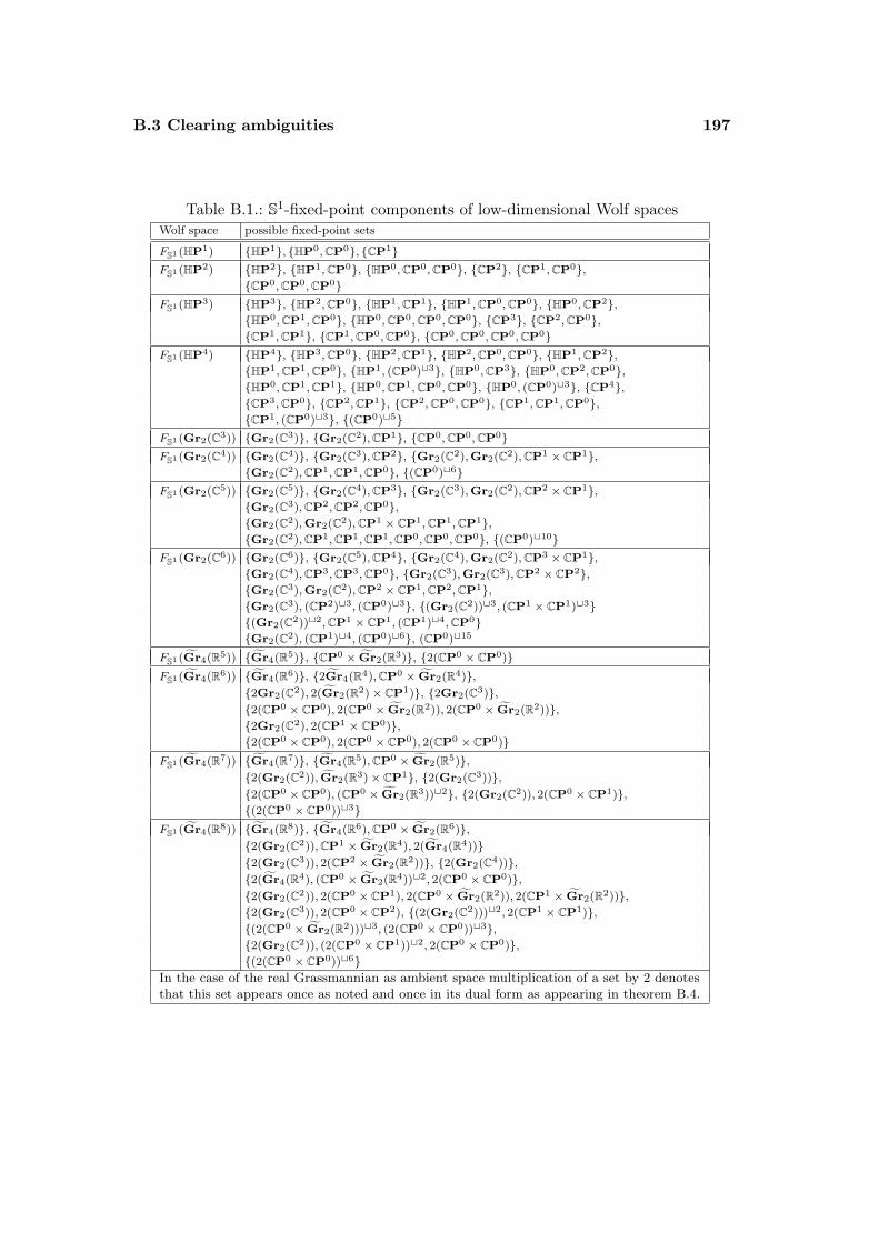
B.3 Clearing ambiguities 197
Table B.1.: S1-fixed-point components of low-dimensional Wolf spacesWolf space possible fixed-point sets
FS1 (HP1) HP1, HP0,CP0, CP1FS1 (HP2) HP2, HP1,CP0, HP0,CP0,CP0, CP2, CP1,CP0,
CP0,CP0,CP0FS1 (HP3) HP3, HP2,CP0, HP1,CP1, HP1,CP0,CP0, HP0,CP2,
HP0,CP1,CP0, HP0,CP0,CP0,CP0, CP3, CP2,CP0,CP1,CP1, CP1,CP0,CP0, CP0,CP0,CP0,CP0
FS1 (HP4) HP4, HP3,CP0, HP2,CP1, HP2,CP0,CP0, HP1,CP2,HP1,CP1,CP0, HP1, (CP0)t3, HP0,CP3, HP0,CP2,CP0,HP0,CP1,CP1, HP0,CP1,CP0,CP0, HP0, (CP0)t3, CP4,CP3,CP0, CP2,CP1, CP2,CP0,CP0, CP1,CP1,CP0,CP1, (CP0)t3, (CP0)t5
FS1 (Gr2(C3)) Gr2(C3), Gr2(C2),CP1, CP0,CP0,CP0FS1 (Gr2(C4)) Gr2(C4), Gr2(C3),CP2, Gr2(C2),Gr2(C2),CP1 × CP1,
Gr2(C2),CP1,CP1,CP0, (CP0)t6FS1 (Gr2(C5)) Gr2(C5), Gr2(C4),CP3, Gr2(C3),Gr2(C2),CP2 × CP1,
Gr2(C3),CP2,CP2,CP0,Gr2(C2),Gr2(C2),CP1 × CP1,CP1,CP1,Gr2(C2),CP1,CP1,CP1,CP0,CP0,CP0, (CP0)t10
FS1 (Gr2(C6)) Gr2(C6), Gr2(C5),CP4, Gr2(C4),Gr2(C2),CP3 × CP1,Gr2(C4),CP3,CP3,CP0, Gr2(C3),Gr2(C3),CP2 × CP2,Gr2(C3),Gr2(C2),CP2 × CP1,CP2,CP1,Gr2(C3), (CP2)t3, (CP0)t3, (Gr2(C2))t3, (CP1 × CP1)t3(Gr2(C2))t2,CP1 × CP1, (CP1)t4,CP0Gr2(C2), (CP1)t4, (CP0)t6, (CP0)t15
FS1 (Gr4(R5)) Gr4(R5), CP0 × Gr2(R3), 2(CP0 × CP0)FS1 (Gr4(R6)) Gr4(R6), 2Gr4(R4),CP0 × Gr2(R4),
2Gr2(C2), 2(Gr2(R2)× CP1), 2Gr2(C3),2(CP0 × CP0), 2(CP0 × Gr2(R2)), 2(CP0 × Gr2(R2)),2Gr2(C2), 2(CP1 × CP0),2(CP0 × CP0), 2(CP0 × CP0), 2(CP0 × CP0)
FS1 (Gr4(R7)) Gr4(R7), Gr4(R5),CP0 × Gr2(R5),2(Gr2(C2)), Gr2(R3)× CP1, 2(Gr2(C3)),2(CP0 × CP0), (CP0 × Gr2(R3))t2, 2(Gr2(C2)), 2(CP0 × CP1),(2(CP0 × CP0))t3
FS1 (Gr4(R8)) Gr4(R8), Gr4(R6),CP0 × Gr2(R6),2(Gr2(C2)),CP1 × Gr2(R4), 2(Gr4(R4))2(Gr2(C3)), 2(CP2 × Gr2(R2)), 2(Gr2(C4)),2(Gr4(R4), (CP0 × Gr2(R4))t2, 2(CP0 × CP0),2(Gr2(C2)), 2(CP0 × CP1), 2(CP0 × Gr2(R2)), 2(CP1 × Gr2(R2)),2(Gr2(C3)), 2(CP0 × CP2), (2(Gr2(C2)))t2, 2(CP1 × CP1),(2(CP0 × Gr2(R2)))t3, (2(CP0 × CP0))t3,2(Gr2(C2)), (2(CP0 × CP1))t2, 2(CP0 × CP0),(2(CP0 × CP0))t6
In the case of the real Grassmannian as ambient space multiplication of a set by 2 denotesthat this set appears once as noted and once in its dual form as appearing in theorem B.4.
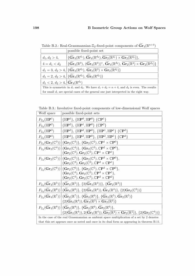
198 B Isometric Group Actions on Wolf Spaces
Table B.2.: Real-Grassmannian-Z2-fixed-point components of Gr4(Rn+4)possible fixed-point set
d1, d2 > 4, Gr4(Rd1), Gr4(Rd2),Gr2(Rd1)×Gr2(Rd2),
4 = d1 < d2 Gr4(R4), (Gr4(R4))∗, Gr4(Rd2), Gr2(R4)×Gr2(Rd2)
d1 = 3, d2 > 4, Gr4(Rd2), Gr2(R3)×Gr2(Rd2)
d1 = 2, d2 > 4, Gr4(Rd2), Gr2(Rd2)
d1 < 2, d2 > 4, Gr4(Rd2)This is symmetric in d1 and d2. We have d1 + d2 = n + 4, and d2 is even. The results
for small di are special cases of the general one just interpreted in the right way.
Table B.3.: Involutive fixed-point components of low-dimensional Wolf spacesWolf space possible fixed-point sets
FZ2(HP1) HP1, HP0,HP0 CP1FZ2(HP2) HP2, HP1,HP0 CP2FZ2(HP3) HP3, HP2,HP0, HP1,HP1 CP3FZ2(HP4) HP4, HP3,HP0, HP2,HP1 CP4FZ2(Gr2(C3)) Gr2(C3), Gr2(C2),CP1 × CP0FZ2(Gr2(C4)) Gr2(C4), Gr2(C3),CP2 × CP0,
Gr2(C2),Gr2(C2),CP1 × CP1FZ2(Gr2(C5)) Gr2(C5), Gr2(C4),CP3 × CP0,
Gr2(C3),Gr2(C2),CP2 × CP1FZ2(Gr2(C6)) Gr2(C6), Gr2(C5),CP4 × CP0,
Gr2(C4),Gr2(C2),CP3 × CP1,Gr2(C3),Gr2(C3),CP2 × CP2
FZ2(Gr4(R5)) Gr4(R5), 2(Gr4(R4)), Gr2(R3)
FZ2(Gr4(R6)) Gr4(R6), 2(Gr4(R4)), Gr2(R4), 2(Gr2(C3))
FZ2(Gr4(R7)) Gr4(R7), Gr4(R6), Gr4(R5), Gr2(R5)2(Gr4(R4)),Gr2(R3)×Gr2(R4)
FZ2(Gr4(R8)) Gr4(R8), Gr4(R6), Gr2(R6),2(Gr4(R4)), 2(Gr4(R4)),Gr2(R4)×Gr2(R4), 2(Gr2(C4))
In the case of the real Grassmannian as ambient space multiplication of a set by 2 denotes
that this set appears once as noted and once in its dual form as appearing in theorem B.11.
C
The Euler Characteristic
In this chapter we apply the last two ones, i.e. chapters A and B, in order to findupper bounds for the Euler characteristic of Positive Quaternion Kahler Manifoldsunder the existence of torus actions. We shall concentrate on low-dimensional cases.Nonetheless the proof for the result in dimension 20 will pave the way towards aninductive approach over all dimensions.
Unfortunately, due to the errors in the classification in dimensions 12—cf. chapter2—we need to suppose that every 12-dimensional Positive Quaternion KahlerManifold is symmetric—or equivalently, that
A(M)[M ] = 0
for every π2-finite 12-dimensional Positive Quaternion Kahler Manifold Mas a general assumption for this chapter.
Thus in order to keep this chapter comparatively short we shall content ourselveswith results that are not optimal yet. The proofs given therefore may be considered asshowcase computations only preceeding an in-depth investigation. However, althougharguments get much more technical and lengthy when optimising the results, theinterested reader will certainly be able to adapt the reasoning we give. Indeed, ourexemplary line of argument will illustrate the techniques to an extent that makes itpossible to continue in this vein. For this we established chapters A and B, whichprovide all the necessary information—beyond our current use.
Let us begin by a depiction of the main idea we use. We shall do so for the specialcase of a 16-dimensional Positive Quaternion Kahler Manifold M and a an effectiveisometric action of a 3-torus T 3 = S1 × S1 × S1, although the arguments may clearlybe adapted to further cases.
Main Idea. The rational cohomology of M is concentrated in the fixed point setMT 3
—cf. theorem [10].VII.1.6, p. 374. That is, in particular χ(M) = χ(MT 3). As
χ(M) > 0 (cf. 1.13) there is a T 3-fixed-point x ∈ M . By means of the isotropy
200 C The Euler Characteristic
representation at x and by the canonical projection Z2 → Sp(1)→ SO(3) we obtainthe homomorphism
ϕ : T 3 → Sp(4)Sp(1)p−→ SO(3)
Thus by consideration of rank we obtain that there is a T 2⊆ kerϕ. Consider theZ2-subtorus T 2
Z2⊆T 2. Hence every involution Z2⊆T 2
Z2fixes a quaternionic component
at x. A combinatorial argument yields that there is always an involution in T 2Z2
thatfixes an at least eight-dimensional (quaternionic) component Nx (cf. page 20).
Inductively, we construct a sequence of quaternionic fixed-point components Ni:Choose a T 3-fixed point x1 and construct the Z2-fixed point component N1 := Nx1 asabove. Now choose a point x2 ∈MT 3 \N1 with corresponding component N2 := Nx2 .We proceed by iteratively choosing a point xi ∈ MT 3 \ N1 ∪ · · · ∪ Ni−1 and byforming the component Ni := Nxi .
By a Fraenkel-type argument (cf. theorem [19].0.1, p. 151) we obtain that any twoquaternionic submanifolds of M intersect provided that their dimension sum is atleast dimM . Thus the involutions that fix Ni and Nj for i < j are distinct elementsof T 3: Since dimNi ≥ 8 and dimNj ≥ 8, we clearly obtain that Ni ∩Nj 6= ∅. So ifboth components are fixed by the same involution, they are necessarily identical andxj 6∈MT \ N1 ∪ · · · ∪Ni ∪ · · · ∪Nj−1 contradicting the construction.
The number of different involutions in T 3Z2
is given by 23−1 = 7. Hence the sequenceof components Ni we constructed above necessarily is finite and consists of the elements
N1, N2, N3, N4, N5, N6, N7
at most.These components are eight-dimensional or twelve-dimensional Positive Quaternion
Kahler Manifolds (cf. page 20). By our general assumption for this chapter all thesemanifolds are symmetric spaces. Consequently, by corollary A.2 we see that theirEuler characteristic is restricted by χ(Ni) ≤ 6 from above unless Ni
∼= Gr2(C5) forsome 1 ≤ i ≤ 7. If this is the case, however, the connectivity lemma 1.20 implies thatthe inclusion Ni →M is 3-connected, whence π2(M) = π2(Ni) = Z. Thus by corollary1.12 we deduce that M ∼= Gr2(C6). So, in total, we may suppose that
χ(M) ≤7∑i=1
χ(Ni) = 7 · 6 = 42
One now proceeds by taking into account the various intersections between theNi-components. This will reduce the Euler characteristic bound even further.
We remark that a 16-dimensional Positive Quaternion Kahler Manifold admits aneffective isometric action of a 2-torus T 2 by theorem 1.18 and by the classification ofsimple Lie groups (cf. table 1.3).
C The Euler Characteristic 201
We now want to illustrate how to reduce the upper bound of the Euler characteristicby taking into account the several intersections of the fixed-point components Ni.We shall do so in the case of an effective isometric 4-torus action in order to keepthe reasoning rather short. Similar results may equally be obtained by means of aT 3-action only.
Lemma C.1. A component of the intersection of two 12-dimensional (quaternionic)Z2-fixed-point components N1 6= N2 (belonging to different involutions contained inT 3) of M16 is a quaternionic isometric Z2-fixed-point component (of N1) of dimension8.
Proof. Let the components N1, N2 belong to the involutions a, b ∈ T 3. As a and bcommute, we see that b restricts to an action on the fixed-point set Ma of a. Moreover,the map b preserves path-components: Choose an arbitrary element g ∈ T 3. Thenthere is a path s : [0, 1]→ T 3 with s(0) = id, s(1) = g. Thus we obtain the path
[0, 1]→Ma : t 7→ (s(t))(x)
from x to g(x) for x ∈Ma. This implies that the action of g—and actually the one ofthe whole T 3—restricts to an action on Ni. So does the action of b in particular.
Hence a component N of the intersection N1 ∩N2 is a component of the action of bon N1. As N2 is quaternionic, the morphism
Z2b → Sp(4)Sp(1)→ SO(3)
(induced by the isotropy representation in a point x ∈ N ⊆M and the canonicalprojection) is trivial. As the inclusion of Sp(3)Sp(1) → Sp(4)Sp(1) is the canonicalblockwise one, we see that also the map Z2b → Sp(3)Sp(1) → SO(3) is trivial inx ∈ N ⊆N1. Thus the fixed-point component N of the action of b on N1 is quaternionic.That is, a component of N1 ∩N2 is quaternionic.
The isotropy representation (in M) of a respectively b in a point x ∈ N (withoutrestriction) is given by (1, 1, 1,−1) and by (1, 1,−1, 1) respectively; i.e. infinitesimally,the components N1 and N2 share two “quaternionic directions”. Thus we computethe dimension of the intersection component N as dim N = 2 · 4 = 8.
Generalisations of this lemma to different components and higher dimensions areobvious. So for example we directly see that the intersection of a 12-dimensional compo-nent and an 8-dimensional quaternionic component (in M16) consists of 4-dimensionalquaternionic Z2-fixed-point-components—unless the 8-dimensional component is con-tained in the 12-dimensional one.
Proposition C.2. Let M be a Positive Quaternion Kahler Manifold with an effectiveisometric T 3-action. If there is a Z2-subgroup of T 3 fixing a 12-dimensional component,then M ∈ HP4,Gr2(C6).
202 C The Euler Characteristic
Proof. In order to prove the result we shall show that if there is a 12-dimensional Z2-component N12, the Euler characteristic of M is smaller than 12 unlessM ∈ HP4,Gr2(C6). This will yield a contradiction.
As we described when depicting the main idea, we cover the T 3-fixed-point set by thecomponents N1, . . . , N7. By dimension, the component N12 is necessarily quaternionic.So suppose N1 = N12. By our general assumption N1 is symmetric. We suppose thatN1∼= Gr4(R7) and shall lead this to a contradiction.
Step 1. We shall see that under the assumption N1∼= Gr4(R7) the Euler charac-
teristic of M is bounded from above by χ(M) < 12.Case 1. Suppose there is another 12-dimensional component N2 6= N1. By lemma
C.1 the intersection N1 ∩N2 is an 8-dimensional Z2-component of N1∼= Gr4(R7). We
now apply the classification of Z2-fixed-point components as elaborated in chapterB. By table B.3 we see that an intersection component N ⊆N1 ∩N2 is isometric toN ∼= Gr4(R6). Since
χ(Gr4(R6)) = 6 = χ(Gr4(R7))
we realise that the cohomology of N2 is already concentrated in N ; i.e. that
MT 3 ∩N2⊆ N ⊆N1
This implies that the components N1, N3, . . . , N7 already cover MT 3.
Case 2. Thus we may assume that there are at most seven components Ni and atmost one of them, namely N1, is of dimension 12—the other ones satisfying dimNi = 8for i 6= 1.
Every 8-dimensional component Ni (for i > 1) intersects with N1 = N12 in a4-dimensional Z2-components unless it is contained in N12. We clearly may neglectthe case of the inclusion Ni⊆N1.
As such a 4-dimensional component is a Z2-component of N1∼= Gr4(R7), table
B.3 yields that it is isometric to HP1. Consequently, as the 4-dimensional compo-nent equally is a Z2-component of the 8-dimensional component Ni, the table yieldsthat Ni
∼= HP2. (For this we make use of the additional information—cf. theorem[73].8.2, p. 537—that Gr2(C3) is the only 4-dimensional quaternionic submanifoldthat G2/SO(4) admits.)
Thus we compute
χ(M) ≤7∑i=1
χ(Ni) = χ(Gr4(R7)) + 6 · (χ(HP2)− χ(HP1)) = 12(C.1)
C The Euler Characteristic 203
We shall now show that the components Ni∼= HP2 (for i > 1) do intersect outside
of N1. This will decrease the upper bound of the Euler characteristic below thecrucial value of 12. We may assume that there are exactly seven components Ni asotherwise the upper bound for the Euler characteristic equally is smaller than 12. Dueto Fraenkel the components Ni (for 1 < i ≤ 7) intersect pairwise.
Suppose all the points of intersection lie in N1. Hence such a point x is an intersectionpoint of at least two 8-dimensional components and the 12-dimensional component N1.Thus the isotropy representation of T 3
Z2in such a point without restriction is given by
(1, 1, 1,−1), (−1,−1, 1, 1), (−1, 1,−1, 1), (−1,−1, 1,−1), (1,−1,−1, 1),(C.2)(−1, 1,−1,−1), (1,−1,−1,−1)
as a direct check shows. Indeed, we focused on the only case possible under theabsence of further 12-dimensional components. Actually, in case 1 we dealt with thesituation of more than one 12-dimensional component and we reduced it to the case ofone 12-dimensional component and only six 8-dimensional ones; this yields a boundwhich is smaller than 12. (As for the notation: We consider a vector—i.e. for example(1, 1, 1,−1)—as a diagonal matrix—i.e. in the example as diag(1, 1, 1,−1)—in Sp(4).The representation of each involution is trivial on the Sp(1)-factor.)
Hence all these points are isolated fixed-points of T 3Z2
on M in which exactly three 8-dimensional components intersect. Without restriction, in the point x we assume thesethree components to be N2, N3 and N4. Let us now consider the intersection of N5 withN2. By assumption there is a point x′ ∈ N1∩N2∩N5 with the representation of T 3
Z2in
x′ being given by (C.2). Thus in x as well as in x′ every involution in T 3Z2
—other thanthe involution belonging to N1—restricted to an action on N1 fixes a four-dimensionalcomponent on N1
∼= Gr4(R7). By table B.3 such a component necessarily is isometricto HP1. In particular, we obtain the following: The involution belonging to N5 fixes afour-dimensional component (in M) in x and an eight-dimensional component (in M)in x′. Restricted to an action on N1 this involution fixes a four-dimensional componentin x (in N1) and another now necessarily distinct four-dimensional component in x′
(in N1). Thus the involution fixes two four-dimensional quaternionic components onN1. By table B.3 this is not possible.
So there are components Ni 6= Nj (with i, j ≥ 2) that do intersect outside of N1 ina component N ⊆Ni ∩Nj . The Euler characteristic of this component was countedtwice in C.1. So we obtain a refinement of (C.1):
χ(M) ≤ χ(Gr4(R7)) + 6 · (χ(HP2)− χ(HP1))− χ(N) ≤ 12− 1 = 11
204 C The Euler Characteristic
Step 2. So in any case we reduced the Euler characteristic χ(M) to a value below12. However, observe that by formula (1.2) combined with Hard-Lefschetz (cf. 1.13)and by excluding the special case (b4, b6, b8) = (2, 1, 2) via theorem [38].1.1, p. 2,the smallest Euler characteristic that may be realised by a rationally 3-connected16-dimensional Positive Quaternion Kahler Manifold other than HP4 comes from thetriple (b4, b6, b8) = (3, 0, 4). It is given by χ(M) = 12.
Combining this with the information obtained in step 1 we conclude thatN1 6∼= Gr4(R7). By our general assumption on symmetry in dimension 12 thisimplies that N1 ∈ HP3,Gr2(C5). By the connectivity lemma 1.20 this implies thatM ∈ HP4,Gr2(C6).
The next proposition is an important step for restricting the Euler characteristic inthe case of a T 3-action. If we are even given a T 4-action—we shall content ourselveswith this stronger assumption—it will already yield a suitable bound.
Proposition C.3. Suppose M16 admits an effective isometric action by a 3-torus T 3.Assume further that there is a T 3-fixed-point where the map
ϕ : T3 → Sp(4)Sp(1)→ SO(3)
induced by the isotropy representation is trivial. Then we obtain
χ(M) ≤ 15
Proof. Following our main idea we consider the isotropy representations of thethree-torus T 3 in its fixed-points. In each such point we obtain a T 2-subtorus, theinvolutions of which fix quaternionic components. We have |T 3
Z2| = 8. So we cover the
T 3-fixed-point set by the components N1, . . . , N7 (with dimNi ≥ 8) as depicted. Byproposition C.2 we may assume that none of the Ni has dimension 12; i.e. we havethat dimNi = 8 for 1 ≤ i ≤ 7.
By the assumption in the assertion there is a T 3-fixed-point x in which everyinvolution in T 3
Z2has a representation in Sp(4). A combinatorial argument then yields
that in x this representation—in the absence of 12-dimensional components—is givenby
(1, 1,−1,−1), (−1,−1, 1, 1), (−1, 1, 1,−1), (1,−1, 1,−1), (−1, 1,−1, 1),(C.3)(1,−1,−1, 1), (−1,−1,−1,−1)
So there are six 8-dimensional components N1, . . . , N6 intersecting in x—we let N1
correspond to (1, 1,−1,−1) and so forth.Let N1 respectively N2 correspond to the involution represented by (1, 1,−1,−1)
respectively by (−1,−1, 1, 1). The Euler characteristic concentrated in N1 ∪ N2 isrestricted by 6+6−1 = 11, since χ(Ni) ≤ 6 by corollary A.2. Every further component
C The Euler Characteristic 205
N3, . . . , N6 intersects both with N1 and N2 in a 4-dimensional component by (C.3).These 4-dimensional pairwise distinct intersection components are represented in x by
(1,−1,−1,−1), (−1, 1,−1,−1), (−1,−1, 1,−1), (−1,−1,−1, 1)
and we shall denote them by N1, N2, N3, N4 (in this order).
Case 1. Suppose that there exist i, j for 1 ≤ i < j ≤ 4 with x ( Ni ∩ Nj . Onthe analogy of lemma C.1 we see that the intersection Ni ∩ Nj consists of isolatedZ2-fixed-points in Ni. That is, the involution corresponding to Nj has at least twoisolated fixed-points when restricted to an action on Ni. By table B.3 the only 4-dimensional Wolf space that admits an involution (contained in a torus) with twoisolated fixed-points is HP1. Thus we obtain that Ni
∼= HP1. By table B.3 weknow that the only 8-dimensional Wolf space that admits a Z2-fixed-point componentisometric to HP1 is HP2. (Again we make use of the fact that G2/SO(4) does notadmit HP1 as a quaternionic submanifold by theorem [73].8.2, p. 537.)
Without restriction we suppose i = 1. Then N1∼= HP1. Consequently, the
componentN1 is isometric to HP2. A 4-dimensional quaternionic Z2-component of HP2
is isometric to HP1 by table B.3. Thus also N2∼= HP1. This again implies N4
∼= HP2
and N6∼= HP2. Continuing in this fashion we obtain that N1, . . . , N6
∼= HP2.Thus we see that the Euler characteristic concentrated in N1 ∪ N2 is restricted
from above by 3 + (3 − 1) = 5. The components Ni∼= HP3 for 3 ≤ i ≤ 6 intersect
with either N1 or N2 in an Nj∼= HP1. Thus the Euler characteristic concentrated
in N1 ∪ · · · ∪ N6 is restricted from above by 5 + 4 · (3 − 2) = 9. Hence the Eulercharacteristic concentrated in N1 ∪ . . . ∪N7 is restricted by 9 + 6 = 15.
Case 2. Suppose that for all i, j with 1 ≤ i < j ≤ 4 we have x = Ni ∩ Nj . As wehave seen the Euler characteristic concentrated in N1 ∪N2 is restricted by 11. Everyfurther component Ni for 3 ≤ i ≤ 6 intersects both with N1 and N2 in one of theNj , Nk with 1 ≤ j, k ≤ 4 respectively. Since Nj ∩ Nk = x, we see that the Eulercharacteristic concentrated in N1 ∪ · · · ∪N6 is restricted by
(χ(N1) + χ(N2)− χ(x)) +6∑i=3
χ(Ni)
− (χ(N2) + χ(N3)− χ(x))− (χ(N1) + χ(N3)− χ(x))(C.4)
− (χ(N2) + χ(N4)− χ(x))− (χ(N1) + χ(N3)− χ(x))≤11 + 4 · (6− (3 + 3− 1))=15
206 C The Euler Characteristic
Indeed, if there is an Ni isometric to G2/SO(4), then it intersects with another eight-dimensional component in an Nj
∼= Gr2(C3). Consequently, its Euler characteristic isalready concentrated in the intersection Nj . Thus a similar refined inequality holds.
If there is a component Ni∼= HP2, then we see that there are two Nj and Nk that
are Z2-fixed point components of Ni (for two different involutions). According to tableB.3 they are homothetic to Nj , Nk
∼= HP1 each. Moreover, table B.3 gives that every8-dimensional component Nl they are contained in is homothetic to HP2. Iterativelycontinuing in this fashion we see that Ni
∼= HP2 for all 1 ≤ i ≤ 6. Consequently,the Euler characteristic concentrated in N1 ∪ N2 is 3 + (3 − 1) = 5. Every furthercomponent Ni for 3 ≤ i ≤ 6 intersects both with N1 and with N2 in one of theNj , Nk with 1 ≤ j, k ≤ 4 respectively. Thus the Euler characteristic concentrated inN1 ∪ . . . ∪N6 is restricted by
(χ(N1) + χ(N2)− χ(x)) +6∑i=3
χ(Ni)
− (χ(N2) + χ(N3)− χ(x))− (χ(N1) + χ(N3)− χ(x))− (χ(N2) + χ(N4)− χ(x))− (χ(N1) + χ(N3)− χ(x))≤5 + 4 · (3− (2 + 2− 1))=5
Thus the Euler characteristic concentrated in N1 ∪ · · · ∪ N7, i.e. the number χ(M)itself, is restricted by χ(M) ≤ 5 + 6 = 11 and we are done.
Hence we may assume in the following that Ni∼= Gr4(R6) for 1 ≤ i ≤ 6.
If there is no seventh component N7, we are done. Otherwise, we now also takeintersections with the seventh component N7 into account.
Clearly, by Fraenkel N7 intersects with each of N1, . . . , N6.Case 2.1. Suppose there is a point x′ with x′ ∈ N7 ∩Ni ∩Nj with i < j < 7. The
existence of these three 8-dimensional components requires the isotropy representationin x′ to be one out of two possibilities:
Case 2.1.1. Assume the isotropy representation of T 3 to be characterized bykerϕ = T 2 with the Z2-subtorus of this T 2 being represented by
(1, 1,−1,−1), (−1, 1, 1,−1), (−1, 1,−1, 1)
These representations correspond to the components N7, Ni and Nj . Thus thecommon intersection component of N7, Ni and Nj is 4-dimensional. This impliesthat the involution corresponding to N7 fixes an isolated fixed-point on Ni in x
C The Euler Characteristic 207
whereas it fixes a four-dimensional quaternionic submanifold of Ni in x′. Accordingto table B.3 there is no classical Wolf space of dimension eight that permits such aninvolution other than Ni
∼= HP2—the subcase we ruled out at the beginning of case 2.Equally, the space G2/SO(4) cannot permit such an involution as the 4-dimensionalfixed-point component is necessarily Gr2(C3)—cf. [73].8.2, p. 537—whence the Eulercharacteristic concentrated in the Z2-fixed-point set would be equal to or bigger thanχ(Gr2(C3)) + χ(x) = 3 + 1 = 4.
Thus this case actually cannot occur.Case 2.1.2. Assume kerϕ = T 3 and suppose the isotropy representation of T 3
Z2in
x′ to be given by
(1, 1,−1,−1), (−1,−1, 1, 1), (−1, 1, 1,−1), (1,−1, 1,−1), (−1, 1,−1, 1),(1,−1,−1, 1), (−1,−1,−1,−1)
Let Nk denote the component corresponding to the involution represented by(−1, 1, 1,−1) in x′. The involution belonging to N7 is represented by(−1,−1,−1,−1) in x and by (1, 1,−1,−1) in x′ without restriction. Thus it fixes a4-dimensional component around x′ in Nk and it has x as an isolated fixed-point in Nk.As in case 2.1.1 this leads to Nk
∼= HP2, which is impossible by assumption. Hencethis case cannot occur either.
Case 2.2. So we may assume that there is no triple intersection of the componentsNi for 1 ≤ i ≤ 7, i.e. whenever x′ ∈ Ni ∩Nj with 1 ≤ i < j ≤ 7 there is no k 6∈ i, jwith 1 ≤ k ≤ 7 and x′ ∈ Nk.
By Fraenkel the component N7 intersects with each of the components N1, . . . , N6.By assumption these intersections now have to be pairwise disjoint. The Euler charac-teristic concentrated in each intersection component is at least one. We have at leastsix different intersection components N1 ∩N7, . . . , N6 ∩N7. The Euler characteristicof N7 is at most χ(N7) ≤ 6. These facts imply that the Euler characteristic of N7
already is concentrated in N1 ∪ · · · ∪N6, i.e. by equation (C.4) we obtain
χ(M) ≤ 15 + χ(N7)−6∑i=1
χ(Ni ∩N7) = 15
This proves the assertion.
Together with our general assumption of symmetry in dimension 12 this propositiondirectly leads to
Theorem C.4. A 16-dimensional Positive Quaternion Kahler Manifold M admittingan isometric action of a 4-torus satisfies
χ(M) ∈ 12, 15
208 C The Euler Characteristic
and
(b4, b6, b8) ∈ (3, 0, 4), (3, 2, 3)
unless it is necessarily symmetric, i.e. M ∈ HP4,Gr2(C6).
Proof. The map
ϕ : T 4 → Sp(4)Sp(1)p−→ SO(3)
induced by the isotropy representation at a T 4-fixed-point x in M satisfies T 3⊆ kerϕfor some subgroup T 3⊆T 4. Hence for the action of this T 3 the prerequisites ofproposition C.3 are satisfied. Consequently, the Euler characteristic of M is restrictedfrom above by
χ(M) ≤ 15
By corollary 1.12 we may suppose M to be rationally 3-connected. Hence by theorem1.13 and in particular by equation (1.2) we obtain the following possibilities for theBetti numbers (b4, b6, b8):
(b4, b6, b8) ∈ (1, 0, 1), (2, 1, 2), (3, 0, 4), (3, 2, 3)
If b4 = 1 theorem 1.15 yields that M ∼= HP4. By [38].1.1, p. 2, the configuration (2, 1, 2)cannot occur. If (b4, b6, b8) = (3, 0, 4), then χ(M) = 12. In the case (b4, b6, b8) = (3, 2, 3)the Euler characteristic is given by χ(M) = 15.
In the case of a T 3-action only a similar theorem can be proved by a deeper analysisof intersections of Z2-fixed-point components.
We remark that χ(Gr4(R8)) = 12 and that χ(Gr2(C6)) = 15—cf. corollary A.2.This shows that the upper bound we found is very good.
The next theorem paves the way for an inductive generalisation over all dimensions.In order to establish a bound for the Euler characteristic of the Positive QuaternionKahler Manifold M4n we shall not assume all Positive Quaternionin Kahler Manifoldsin dimensions smaller than 4n to be symmetric. The proof provides an argument thatnonetheless makes it possible to find an upper bound.
Theorem C.5. A Positive Quaternion Kahler Manifold M of dimension dimM = 20that admits an effective isometric action by a 4-torus T 4 satisfies
χ(M) ≤ 225
C The Euler Characteristic 209
Proof. We adapt the main idea presented above to dimension 20: In a T 4-fixed-point we consider the isotropy representation of T 3
Z2⊆T 3⊆ kerϕ (with the notation
from above). We realise that we can always find an involution that fixes an at least12-dimensional quaternionic component. Since |T 4
Z2| = 24, we thus know that the
fixed-point set MT 4can be covered by at most 24− 1 = 15 quaternionic Z2-fixed-point
components
N1, . . . , N15
satisfying dimNi ≥ 12. Thus the Euler characteristic of M is restricted by
χ(M) ≤15∑i=1
χ(Ni)
If dimNi = 12, we cite χ(Ni) ≤ 10 from corollary A.2 due to our general assumptionof symmetry in dimension 12.
Suppose now there is an Ni of dimension dimNi = 16. Assume that Ni is fixed bythe involution a ∈ T 3
Z2. Since a commutes with T 4, the action of T 4 restricts to an
action on the fixed-point set Ma. Moreover, in the proof of lemma C.1 we have seenthat the action of T 4 restricts to an action on Ni.
If this action, T 4 y Ni, is not almost effective, i.e. if there is an S1-subgroup ofT 4 fixing Ni, then Ni is a codimension four S1-fixed-point component of M . Thusby theorem [20].1.2, p. 2, we obtain that M ∼= HP5 or M ∼= Gr2(C7). Otherwise, ifT 4 acts almost effectively, we may apply the whole reasoning to dimension 16 withthe action of a 4-torus. This was done in theorem C.4, which yields the upper boundχ(Ni) ≤ 15. Hence, in total, we obtain:
χ(M) ≤ 15 · 15 = 225
Taking into account the various intersections of the components Ni again permitsto reduce the upper bound for χ(M) tremendously.
For an iterative approach for χ(M4n) we finally notice the following: In each torus-fixed-point we need to find a Z2-fixed-point component Ni that has dimension at least2n. For this it is sufficient for the torus to have a rank lying in O(log2 n)—this caneasily be made more precise—as a combinatorial argument shows.

D
The Elliptic Genus of WolfSpaces
As we remarked in chapter 2, it remains a challenging task to prove the vanishingof the A-genus on Positive Quaternion Kahler Manifolds M that are not necessarilyspin but π2-finite. This question can be seen in the larger context of a description ofthe elliptic genus Φ(M). Indeed, Φ(M) admits an expansion as a power series whichcontains A(M)[M ] as a first coefficient (cf. [39]).
We shall provide this description on Wolf spaces M . We ignore the complexGrassmannian, as b2(Gr2(Cn+2)) = 1. Stepping through the list of Wolf spaces(cf. table 1.2) then basically yields four different cases:
• The Wolf space is M ∼= HPn.
• The Wolf space is exceptional.
• We have M ∼= Gr4(Rn+4) for even n ≥ 2.
• We have M ∼= Gr4(Rn+4) for odd n ≥ 1.
Clearly, the quaternionic projective space is spin. (Moreover, in odd quaternionicdimensions it is the only Positive Quaternion Kahler Manifold that is spin.) Theexceptional Wolf spaces—except for F4/Sp(3)Sp(1)—as well as Gr4(Rn+4) for evenn ≥ 2 have even quaternionic dimension. Thus they are spin manifolds M .
So a reasoning due to [39] identifies the equivariant elliptic genus Φ(M, g) of aninvolution g with the one of the transversal self-intersection, Φ(Mg t Mg, g), of thefixed-point set of g. The rigidity of the elliptic genus on spin manifolds yields
Φ(M) = Φ(M, g) = Φ(Mg t Mg, g)
This permits an approach inductive on dimension. Due to the theorem on [39], p. 321this leads to
Φ(M) = sign(M) = b2n(M)
212 D The Elliptic Genus of Wolf Spaces
(If M is a Positive Quaternion Kahler Manifold of even quaternionic dimension, itsintersection form is positive definite–cf. 1.16. Otherwise, if M is spin and of oddquaternionic dimension, we have M ∼= HPn and sign(M) = −b2n = 0.) This gives acomplete picture in the spin case.
Thus only the cases of the real Grassmannian Gr4(Rn+4) with odd n and of theexceptional space F4/Sp(3)Sp(1) remain. We shall prove the vanishing of Φ(Gr4(Rn+4)in this case. Compare also the result on [36], p. 202–203, which was obtained bycomputations on the twistor space. However, we shall give a more direct reasoning. Forthe exceptional Wolf space we quote the computations on [36], p. 204–205, althoughour method applies to this case as well.
For the convenience of the reader we shall illustrate a method of direct computation—following [39] once more—in the eight-dimensional case. This will serve as a showcasecomputation for the more general case of arbitrary odd quaternionic dimension, whichwe shall deal with later. Alongside this model computation we shall establish necessaryfacts and notation. As a general reference on Index Theory we recommend thetextbooks [40] and [52].
We have
Gr4(Rn+4) =SO(n+ 4)
SO(n)× SO(4)
whence Gr4(R6) = SO(6)SO(2)×SO(4) . The positive roots of SO(6) (corresponding to the
standard maximal torus) are given by
x1 ∓ x3, x1 ∓ x2, x2 ∓ x3
where xi is dual to the i-th factor of the maximal torus. The positive roots of thedenominator SO(2)×SO(4) are given by x2∓x3, whence the complementary positiveroots are the
x1 ∓ x3, x1 ∓ x2
(Clearly, we have that 2|x1 ∓ x3, x1 ∓ x2| = dim Gr4(R6).)The Weyl group of SO(2n + 1) is given by the group G of permutations of
−n, . . . ,−1, 1, . . . , n equivariant under multiplication with (−1)—cf. [11], p. 171.The Weyl group of SO(2n) is the subgroup SG of even permutations. We obtain the
D The Elliptic Genus of Wolf Spaces 213
coset
W(
SO(6)SO(2)× SO(4)
):=
W(SO(6)W(SO(2)× SO(4))
=SG(3)
SG(1)× SG(2)
=SG(3)SG(2)
∼=1 0 0
0 1 00 0 1
,
−1 0 00 −1 00 0 1
,
0 1 01 0 00 0 1
,
0 −1 0−1 0 00 0 1
,
0 1 00 0 11 0 0
,
0 −1 00 0 1−1 0 0
The maximal torus T 3 of SO(6) acts isometrically on SO(6)SO(2)×SO(4) by left-
multiplication. We consider the isometric S1-action induced by the inclusion ofS1 into T 3 by g 7→ (g1, g2, g3), where g is a topological generator of S1.
The fixed-points of this action are isolated and in one-to-one correspondence with
W( SO(6)SO(2)× SO(4)
)The rotation numbers on the tangent space of such a fixed-point are given by evaluationon roots, i.e. the rotation numbers in a point
w ∈W( SO(6)SO(2)× SO(4)
)are given by
〈w(x1 ∓ x2, x1 ∓ x3), φ〉 = w(x1 ∓ x2, x1 ∓ x3)|x1=1,x2=2,x3=3
The orientation in a point is compatible with the orientation of the ambient manifoldif and only if the determinant of the transformation w corresponding to the fixed-pointis positive. (For this consider w as a linear map on the vector space generated by theroots.)
For example, in the identity component we obtain the rotation numbers
x1 ∓ x2, x1 ∓ x3|x1=1,x2=2,x3=3 = −1, 3,−2, 4
whereas in the fixed-point corresponding to−1 0 00 −1 00 0 1
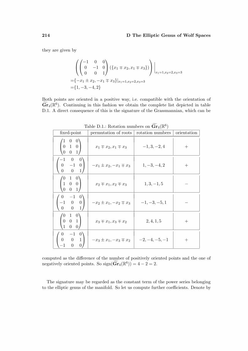
214 D The Elliptic Genus of Wolf Spaces
they are given by−1 0 00 −1 00 0 1
(x1 ∓ x2, x1 ∓ x3)
∣∣∣∣x1=1,x2=2,x3=3
=−x1 ± x2,−x1 ∓ x3|x1=1,x2=2,x3=3
=1,−3,−4, 2
Both points are oriented in a positive way, i.e. compatible with the orientation ofGr4(R6). Continuing in this fashion we obtain the complete list depicted in tableD.1. A direct consequence of this is the signature of the Grassmannian, which can be
Table D.1.: Rotation numbers on Gr4(R6)fixed-point permutation of roots rotation numbers orientation1 0 0
0 1 00 0 1
x1 ∓ x2, x1 ∓ x3 −1, 3,−2, 4 +
−1 0 00 −1 00 0 1
−x1 ± x2,−x1 ∓ x3 1,−3,−4, 2 +
0 1 01 0 00 0 1
x2 ∓ x1, x2 ∓ x3 1, 3,−1, 5 −
0 −1 0−1 0 00 0 1
−x2 ± x1,−x2 ∓ x3 −1,−3,−5, 1 −
0 1 00 0 11 0 0
x3 ∓ x1, x3 ∓ x2 2, 4, 1, 5 +
0 −1 00 0 1−1 0 0
−x3 ± x1,−x3 ∓ x2 −2,−4,−5,−1 +
computed as the difference of the number of positively oriented points and the one ofnegatively oriented points. So sign(Gr4(R6)) = 4− 2 = 2.
The signature may be regarded as the constant term of the power series belongingto the elliptic genus of the manifold. So let us compute further coefficients. Denote by
D The Elliptic Genus of Wolf Spaces 215
TC the complexified tangent bundle and set
∧tTC =
4n∑k=0
(∧kTC)tk StTC =∞∑k=0
(SkTC)tk
Recall that the elliptic genus is given by
Φ(X) = sign(X,
∞∏m=1
∧qmTC ·
∞∏m=1
SqmTC
)(D.1)
where X is a compact oriented 4n-dimensional manifold. In the same way one obtainsan equivariant formula when replacing formal roots by equivariant formal roots. Oneobtains the following form:
Φ(X, g) =∞∑m=0
sign(X,Rm, g)qm
where we focus on g being a topological generator of S1. The bundles Rm are thecoefficient bundles arising from (D.1). So we may compute them by means of thesubsequent equation.
∞∏m=1
∧qmTC ·
∞∏m=1
SqmTC
=∞∏m=1
∞∑k=0
(∧kTC)(qm)k ·∞∏m=1
∞∑k=0
(SkTC)(qm)k
=(1 + TCq + TC ∧ TCq2 + . . . ) · (1 + TCq
2 + TC ∧ TCq4 + . . . ) · . . .
· (1 + TCq + S2TCq2 + . . . ) · (1 + TCq
2 + S2TCq4 + . . . ) · . . .
=1 + 2TCq + 2(TC + TC ⊗ TC + TC ∧ TC + S2TC)q2
+ (2TC + 4TC ⊗ TC + TC ⊗ TC ⊗ TC + ∧3TC + S3TC)q3 + . . .
This implies in particular that
R0 = 1R1 = 2TC
R2 = 2(TC + TC ⊗ TC)
R3 = 2TC + 4TC ⊗ TC + TC ⊗ TC ⊗ TC + ∧3TC + S3TC
(In degree two we have an exceptional identity T ∧ T + S2T = T ⊗ T .)In general, one may determine sign(X,Rm, g) via a computation on fixed-point
components ν of g:
sign(X,Rm, g) =∑ν
sign(Xgν , Rm, g)
216 D The Elliptic Genus of Wolf Spaces
up to orientation/sign of each summand (cf. [40], 5.8, p. 72). In terms of powerseries one may compute such an expression by replacing the formal roots of the powerseries of the L-genus by equivariant formal roots and by twisting the expression withchg(Rm). (The equivariant Chern character chg(Rm) again results from ch(Rm) byreplacing formal roots xi by the equivariant roots xi + tiz of Rm. Here ti ∈ N0 isthe rotation number of g on the root xi of Rm and z is a formal variable.) In ourcase all the fixed-points of the S1-action on Gr4(R6) are isolated, which simplifies thesituation, since the topology of the fixed-point components—the part in the formulawith rotation number equal to zero—yields a trivial contribution. So we obtain
sign(ν,Rm, g) =∑ν
((∏k>0
dk∏i=1
1 + e−(xi+tkz)
1− e−(xi+tkz)
)· chg(Rm)
)[ν]
=∑ν
±(∏k>0
dk∏i=1
1 + e−tkz
1− e−tkz
)· chg(Rm)(D.2)
The last equation holds, since we evaluate on 0-dimensional isolated fixed-points andtherefore may set the xi to zero. (In this formula xi is always supposed to correspondto a root on which the rotation number is tk.) The ±-sign is chosen according towhether the orientation of the fixed-point is compatible with the orientation of theambient manifold or not.
We need to compute the equivariant Chern characters: Complexification of thetangent bundle T induces an action of g on TC with rotation numbers (ti,−ti) whenti being a rotation number of the action on T at a fixed-point. The Chern characterof a complex bundle of rank m is given by
m∑r=1
eyr
in terms of its formal roots yr. Thus the equivariant Chern character becomes
m∑r=1
etrz+yr(D.3)
With this we compute
chg(TC) =4n∑r=1
etrz+xr + e−trz+xr+n
The additivity and multiplicativity of the Chern character permits us to compute theequivariant Chern characters of the bundles Rm. In order to compute equivariant
D The Elliptic Genus of Wolf Spaces 217
Chern characters of symmetric and exterior powers we use formula (D.3) with theformal roots of SkTC being given by the
yr = xi1 + · · ·+ xir with 1 ≤ i1 ≤ · · · ≤ ik ≤ 2n
The formal roots of ∧kTC are the
yr = xi1 + · · ·+ xir with 1 ≤ i1 < · · · < ik ≤ 2n
From now on let us specialise again to the S1-action φ from above which acts withisolated fixed-points only. Once more, in particular, we therefore may also set theroots xi in the equivariant Chern characters to zero.
We have obtained a formula for the equivariant elliptic genus by means of equivarianttwisted signatures. We have further seen how to compute equivariant Chern characters,which enables us to compute the signatures. Table D.1 now tells us whether theorientation of a fixed-point is compatible with the ambient manifold or not and whatthe rotation numbers on the tangent bundle look like. All this information now issufficient to compute the equivariant elliptic genus.
So compute the twisted equivariant signatures: By ν1, . . . , ν6 we denote the differentfixed-points in the order according to their order of appearance in table D.1. Since therotation numbers in ν1 and ν2, the ones in ν3 and ν4 and the ones in ν5 and ν6 coincideup to sign and since these points have the same orientation, we obtain—irrespectiveof the twisting bundle Rm—that
sign(Gr4(R6)), Rm, g) = sign(ν1, Rm, g) + sign(ν2, Rm, g)− sign(ν3, Rm, g)− sign(ν4, Rm, g)+ sign(ν5, Rm, g) + sign(ν6, Rm, g)
= 2sign(ν1, Rm, g)− 2sign(ν3, Rm, g) + 2sign(ν5, Rm, g)
By means of (D.2) we compute
sign(Gr4(R6), g) = 2 ·(
1 + e1·z
1− e1·z
)(1 + e2·z
1− e2·z
)(1 + e3·z
1− e3·z
)(1 + e4·z
1− e4·z
)− 2 ·
(1 + e1·z
1− e1·z
)(1 + e1·z
1− e1·z
)(1 + e3·z
1− e3·z
)(1 + e5·z
1− e5·z
)+ 2 ·
(1 + e1·z
1− e1·z
)(1 + e2·z
1− e2·z
)(1 + e4·z
1− e4·z
)(1 + e5·z
1− e5·z
)= 2
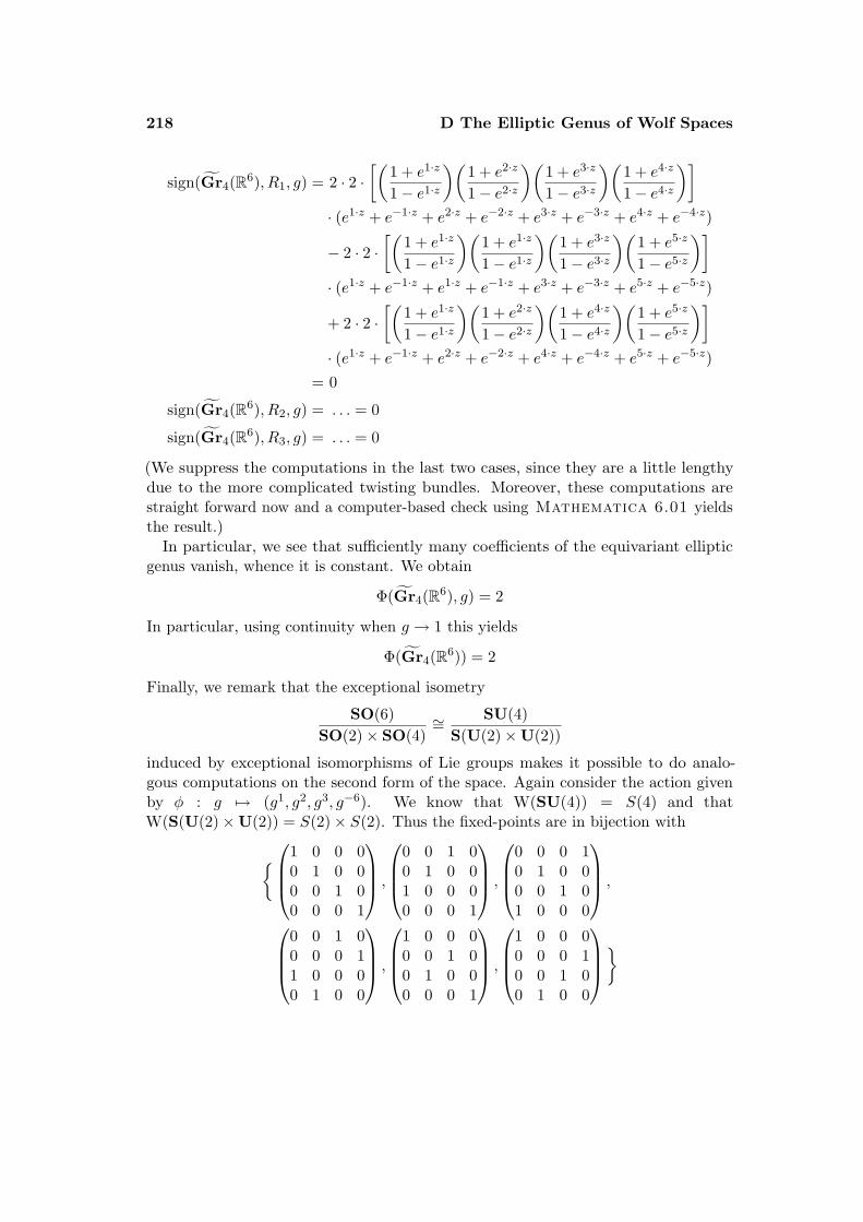
218 D The Elliptic Genus of Wolf Spaces
sign(Gr4(R6), R1, g) = 2 · 2 ·[(
1 + e1·z
1− e1·z
)(1 + e2·z
1− e2·z
)(1 + e3·z
1− e3·z
)(1 + e4·z
1− e4·z
)]· (e1·z + e−1·z + e2·z + e−2·z + e3·z + e−3·z + e4·z + e−4·z)
− 2 · 2 ·[(
1 + e1·z
1− e1·z
)(1 + e1·z
1− e1·z
)(1 + e3·z
1− e3·z
)(1 + e5·z
1− e5·z
)]· (e1·z + e−1·z + e1·z + e−1·z + e3·z + e−3·z + e5·z + e−5·z)
+ 2 · 2 ·[(
1 + e1·z
1− e1·z
)(1 + e2·z
1− e2·z
)(1 + e4·z
1− e4·z
)(1 + e5·z
1− e5·z
)]· (e1·z + e−1·z + e2·z + e−2·z + e4·z + e−4·z + e5·z + e−5·z)
= 0
sign(Gr4(R6), R2, g) = . . . = 0
sign(Gr4(R6), R3, g) = . . . = 0
(We suppress the computations in the last two cases, since they are a little lengthydue to the more complicated twisting bundles. Moreover, these computations arestraight forward now and a computer-based check using Mathematica 6.01 yieldsthe result.)
In particular, we see that sufficiently many coefficients of the equivariant ellipticgenus vanish, whence it is constant. We obtain
Φ(Gr4(R6), g) = 2
In particular, using continuity when g → 1 this yields
Φ(Gr4(R6)) = 2
Finally, we remark that the exceptional isometry
SO(6)SO(2)× SO(4)
∼=SU(4)
S(U(2)×U(2))
induced by exceptional isomorphisms of Lie groups makes it possible to do analo-gous computations on the second form of the space. Again consider the action givenby φ : g 7→ (g1, g2, g3, g−6). We know that W(SU(4)) = S(4) and thatW(S(U(2)×U(2)) = S(2)× S(2). Thus the fixed-points are in bijection with
1 0 0 00 1 0 00 0 1 00 0 0 1
,
0 0 1 00 1 0 01 0 0 00 0 0 1
,
0 0 0 10 1 0 00 0 1 01 0 0 0
,
0 0 1 00 0 0 11 0 0 00 1 0 0
,
1 0 0 00 0 1 00 1 0 00 0 0 1
,
1 0 0 00 0 0 10 0 1 00 1 0 0
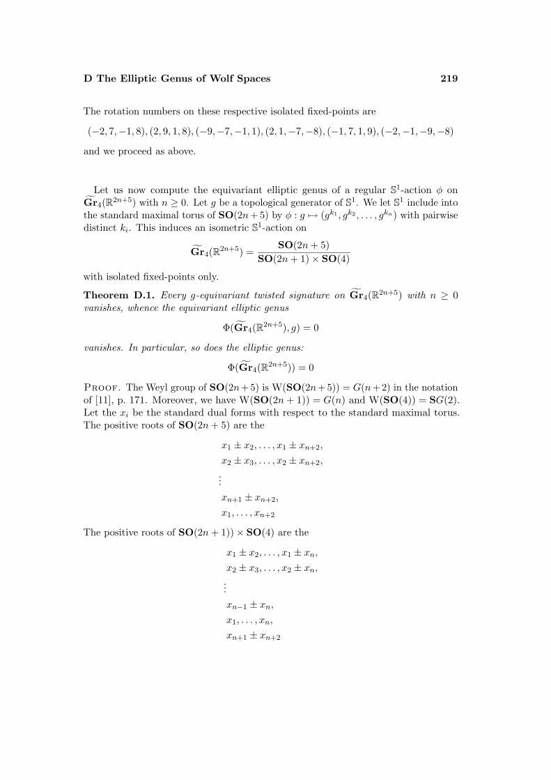
D The Elliptic Genus of Wolf Spaces 219
The rotation numbers on these respective isolated fixed-points are
(−2, 7,−1, 8), (2, 9, 1, 8), (−9,−7,−1, 1), (2, 1,−7,−8), (−1, 7, 1, 9), (−2,−1,−9,−8)
and we proceed as above.
Let us now compute the equivariant elliptic genus of a regular S1-action φ onGr4(R2n+5) with n ≥ 0. Let g be a topological generator of S1. We let S1 include intothe standard maximal torus of SO(2n+ 5) by φ : g 7→ (gk1 , gk2 , . . . , gkn) with pairwisedistinct ki. This induces an isometric S1-action on
Gr4(R2n+5) =SO(2n+ 5)
SO(2n+ 1)× SO(4)
with isolated fixed-points only.
Theorem D.1. Every g-equivariant twisted signature on Gr4(R2n+5) with n ≥ 0vanishes, whence the equivariant elliptic genus
Φ(Gr4(R2n+5), g) = 0
vanishes. In particular, so does the elliptic genus:
Φ(Gr4(R2n+5)) = 0
Proof. The Weyl group of SO(2n+ 5) is W(SO(2n+ 5)) = G(n+ 2) in the notationof [11], p. 171. Moreover, we have W(SO(2n+ 1)) = G(n) and W(SO(4)) = SG(2).Let the xi be the standard dual forms with respect to the standard maximal torus.The positive roots of SO(2n+ 5) are the
x1 ± x2, . . . , x1 ± xn+2,
x2 ± x3, . . . , x2 ± xn+2,
...xn+1 ± xn+2,
x1, . . . , xn+2
The positive roots of SO(2n+ 1))× SO(4) are the
x1 ± x2, . . . , x1 ± xn,x2 ± x3, . . . , x2 ± xn,...xn−1 ± xn,x1, . . . , xn,
xn+1 ± xn+2
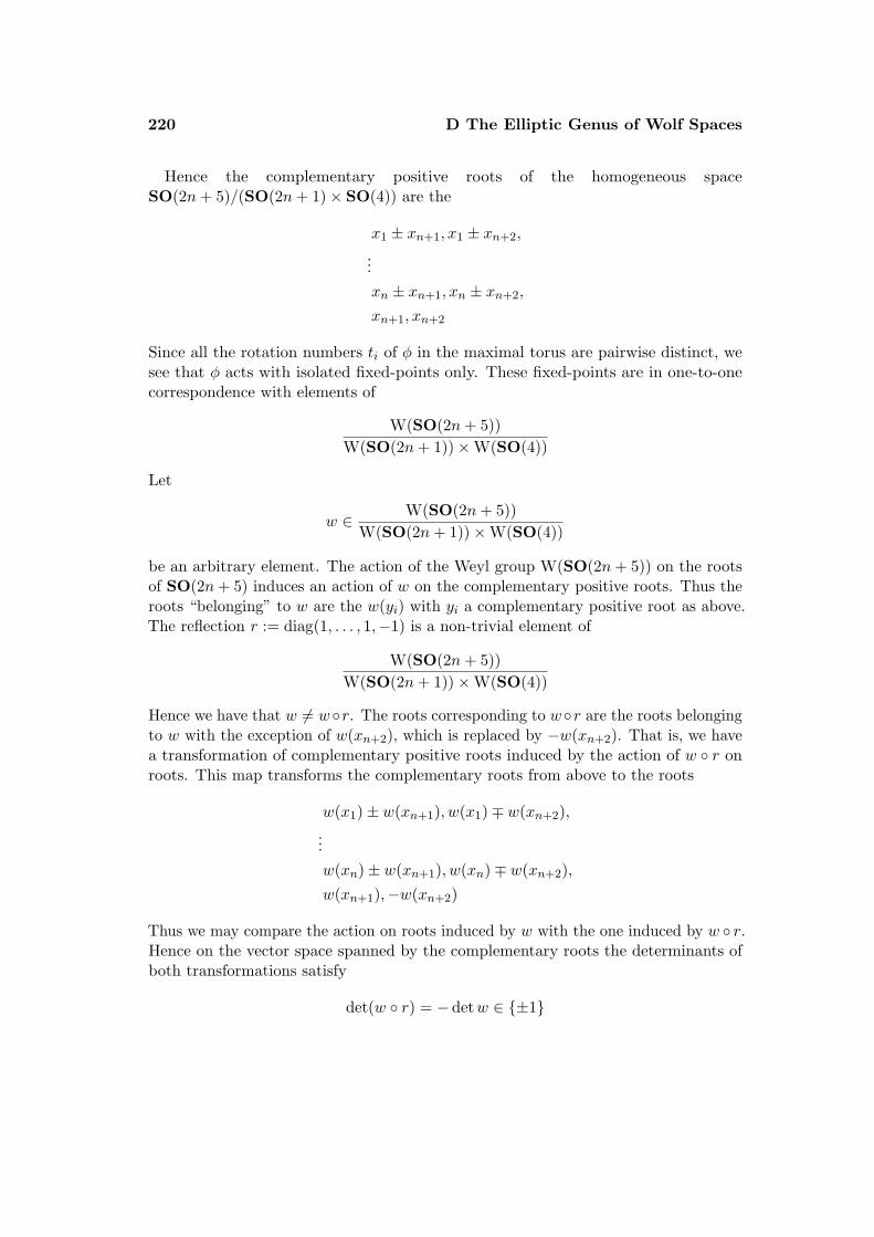
220 D The Elliptic Genus of Wolf Spaces
Hence the complementary positive roots of the homogeneous spaceSO(2n+ 5)/(SO(2n+ 1)× SO(4)) are the
x1 ± xn+1, x1 ± xn+2,
...xn ± xn+1, xn ± xn+2,
xn+1, xn+2
Since all the rotation numbers ti of φ in the maximal torus are pairwise distinct, wesee that φ acts with isolated fixed-points only. These fixed-points are in one-to-onecorrespondence with elements of
W(SO(2n+ 5))W(SO(2n+ 1))×W(SO(4))
Let
w ∈ W(SO(2n+ 5))W(SO(2n+ 1))×W(SO(4))
be an arbitrary element. The action of the Weyl group W(SO(2n+ 5)) on the rootsof SO(2n+ 5) induces an action of w on the complementary positive roots. Thus theroots “belonging” to w are the w(yi) with yi a complementary positive root as above.The reflection r := diag(1, . . . , 1,−1) is a non-trivial element of
W(SO(2n+ 5))W(SO(2n+ 1))×W(SO(4))
Hence we have that w 6= wr. The roots corresponding to wr are the roots belongingto w with the exception of w(xn+2), which is replaced by −w(xn+2). That is, we havea transformation of complementary positive roots induced by the action of w r onroots. This map transforms the complementary roots from above to the roots
w(x1)± w(xn+1), w(x1)∓ w(xn+2),...w(xn)± w(xn+1), w(xn)∓ w(xn+2),w(xn+1),−w(xn+2)
Thus we may compare the action on roots induced by w with the one induced by w r.Hence on the vector space spanned by the complementary roots the determinants ofboth transformations satisfy
det(w r) = −detw ∈ ±1
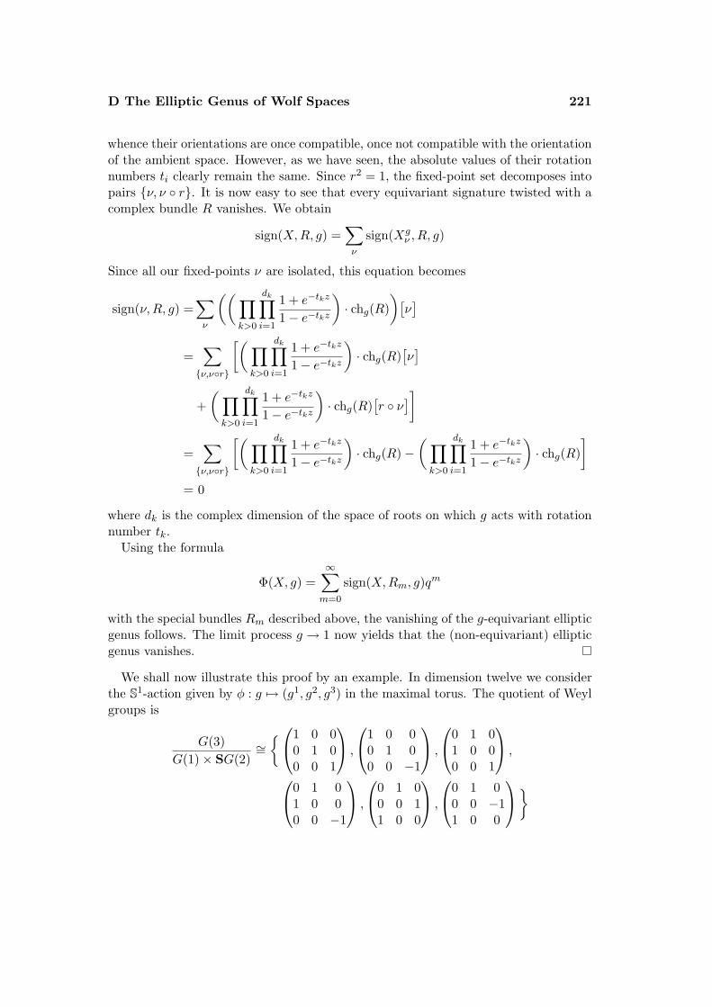
D The Elliptic Genus of Wolf Spaces 221
whence their orientations are once compatible, once not compatible with the orientationof the ambient space. However, as we have seen, the absolute values of their rotationnumbers ti clearly remain the same. Since r2 = 1, the fixed-point set decomposes intopairs ν, ν r. It is now easy to see that every equivariant signature twisted with acomplex bundle R vanishes. We obtain
sign(X,R, g) =∑ν
sign(Xgν , R, g)
Since all our fixed-points ν are isolated, this equation becomes
sign(ν,R, g) =∑ν
((∏k>0
dk∏i=1
1 + e−tkz
1− e−tkz
)· chg(R)
)[ν]
=∑ν,νr
[(∏k>0
dk∏i=1
1 + e−tkz
1− e−tkz
)· chg(R)
[ν]
+(∏k>0
dk∏i=1
1 + e−tkz
1− e−tkz
)· chg(R)
[r ν
]]
=∑ν,νr
[(∏k>0
dk∏i=1
1 + e−tkz
1− e−tkz
)· chg(R)−
(∏k>0
dk∏i=1
1 + e−tkz
1− e−tkz
)· chg(R)
]= 0
where dk is the complex dimension of the space of roots on which g acts with rotationnumber tk.
Using the formula
Φ(X, g) =∞∑m=0
sign(X,Rm, g)qm
with the special bundles Rm described above, the vanishing of the g-equivariant ellipticgenus follows. The limit process g → 1 now yields that the (non-equivariant) ellipticgenus vanishes.
We shall now illustrate this proof by an example. In dimension twelve we considerthe S1-action given by φ : g 7→ (g1, g2, g3) in the maximal torus. The quotient of Weylgroups is
G(3)G(1)× SG(2)
∼=1 0 0
0 1 00 0 1
,
1 0 00 1 00 0 −1
,
0 1 01 0 00 0 1
,
0 1 01 0 00 0 −1
,
0 1 00 0 11 0 0
,
0 1 00 0 −11 0 0
222 D The Elliptic Genus of Wolf Spaces
The complementary positive roots are given by
x1 ± x2, x1 ± x3, x2, x3
Hence the rotation numbers on the different points turn out to be
3,−1, 4,−2, 2, 3 ↔ 3,−1,−2, 4, 2,−33, 1, 5,−1, 1, 3 ↔ 3, 1,−1, 5, 1,−35, 1, 4, 2, 1, 2 ↔ 1, 5, 4, 2, 1,−2
The fixed-point set splits into pairs as indicated. Orientations on the respective pointsin a pair are opposite to one another whereas absolute values of orientation numbersremain identical. Consequently, twisted equivariant signatures vanish and so does theelliptic genus.
E
Indices in Dimension 16
In this chapter we provide index computations in dimension 16. See section 4.1 forthe analogous case of dimension 20.
E.1. Preliminaries
On a 16-dimensional Positive Quaternion Kahler Manifold M the locally-definedcomplex vector bundles E and H are associated to the standard representations ofSp(4) and Sp(1) respectively. We twist the Dirac operator with the bundles
Rp,q =∧p
0E ⊗ SqH
provided 4+p+q is even. Again∧p
0E is the (virtual) bundle∧pE−
∧p−2E. Theorem1.17 yields the relations
ip,q =
0 for p+ q < 4(−1)p(b2p−2 + b2p) for p+ q = 4d for p = 0, q = 6
where d = dim Isom(M) is the dimension of the isometry group of M . Again we shallcompute the indices ip,q for these interesting values of p and q in terms of characteristic
224 E Indices in Dimension 16
classes of the bundles E and H. As in the 20-dimensional case we compute
A(M) =1 +(c2 − 4u
12
)+(
3c22 − c4 − 23c2u+ 42u2
720
)+(
10c32 − 9c2c4 + 2c6 − 115c2
2u+ 48c4u+ 388c2u2 − 432u3
60480
)+(
21c42 − 34c2
2c4 + 5c24 + 13c2c6 − 3c8 − 334c3
2u+ 364c2c4u
3628800+
−103c6u+ 1636c22u
2 − 799c4u2 − 3263c2u
3 + 2497u4
3628800
)ch(E) =8− c2 +
c22 − 2c4
12+−c3
2 + 3c2c4 − 3c6
360+c4
2 − 4c22c4 + 2c2
4 + 4c2c6 − 4c8
20160
ch(H) =2 + u+u2
12+
u3
360+
u4
20160By means of the Clebsch-Gordan formula we compute
i0,0 =c4
2
172800− 17c2
2c4
1814400+
c24
725760+
13c2c6
3628800− c8
1209600− 167c3
2u
1814400+
13c2c4u
129600
− 103c6u
3628800+
409c22u
2
907200− 799c4u
2
3628800− 3263c2u
3
3628800+
2497u4
3628800
i0,1 =c4
2
86400− 17c2
2c4
907200+
c24
362880+
13c2c6
1814400− c8
604800− 17c3
2u
907200+
47c2c4u
907200−
43c6u
1814400− 37c2
2u2
56700+
431c4u2
1814400+
3967c2u3
1814400− 3233u4
1814400
i0,2 =c4
2
57600− 17c2
2c4
604800+
c24
241920+
13c2c6
1209600− c8
403200+
233c32u
604800− 89c2c4u
302400+
19c6u
403200− 211c2
2u2
302400+
89c4u2
134400− 647c2u
3
134400+
211u4
44800
i0,3 =c4
2
43200− 17c2
2c4
453600+
c24
181440+
13c2c6
907200− c8
302400+
583c32u
453600− 493c2c4u
453600+
197c6u
907200+
1277c22u
2
113400− 2209c4u
2
907200+
10207c2u3
907200− 18593u4
907200
i0,4 =c4
2
34560− 17c2
2c4
362880+
c24
145152+
13c2c6
725760− c8
241920+
1033c32u
362880− 449c2c4u
181440+
377c6u
725760+
2129c22u
2
36288− 12127c4u
2
725760+
263233c2u3
725760+
86285u4
145152
i0,6 =7c4
2
172800− 17c2
2c4
259200+
c24
103680+
13c2c6
518400− c8
172800+
2233c32u
259200− 989c2c4u
129600+
857c6u
518400+
57169c22u
2
129600− 71839c4u
2
518400+
4117057c2u3
518400+
24236737u4
518400Again the “indices” i0,1 and i0,3 are to be regarded as formal expressions. Since thesum of their superscripts is not even, they do not necessarily represent indices of
E.1 Preliminaries 225
twisted Dirac operators. As in the 20-dimensional case we compute
ch(∧2
E) =28− 6c2 +c2
2− c3
2
60+
c42
3360− c2c4
30+c2
2c4
630+
c24
504+c6
5− 13c2c6
840+c8
42
ch(∧3
E) =56− 15c2 +5c2
2
4− c3
2
24+
c42
1344+
3c4
2− 5c2c4
24+
41c22c4
5040+
71c24
10080− c6
8
+11c2c6
560− 397c8
1680
ch(∧4
E) =70− 20c2 +5c2
2
3− c3
2
18+
c42
1008+
8c4
3− c2c4
3+
4c22c4
315+
13c24
1260− 2c6
3
+89c2c6
1260+
151c8
315
Again these exterior powers already determine all the higher ones by Hodge ∗-duality.That is, we obtain ∧k
E ∼=∧8−k
E
for 0 ≤ k ≤ 8 and
ch(∧k
E) = ch(∧8−k
E)
respectively
ch(∧k
0E) = −ch(
∧10−k
0E)
and
ip,q = −i10−p,q
In particular, i5,q = 0 for all q ∈ N0, since ch(∧5E) = ch(
∧3E).This enables us to compute the following indices in terms of characteristic numbers.
(Again the “indices” i1,0 and i3,0 are to be regarded as formal expressions.) As wehave seen, as for the first parameter it suffices to compute from p = 0 to p = 4.
i1,0 =1
453600(21c4
2 + 155c24 − 93c8 − 259c3
2u+ 1157c6u− 5209c4u2 + 2497u4
+ c22(−109c4 + 931u2) + c2(−227c6 + 1159c4u− 23u3))
i2,0 =1
403200(63c4
2 + 815c24 + 9591c8 − 602c3
2u− 27189c6u− 2397c4u2 + 7491u4
+ c22(−502c4 + 1148u2) + c2(439c6 + 3652c4u+ 7491u3))
i3,0 =1
75600(21c4
2 + 355c24 − 17853c8 − 159c3
2u+ 2837c6u+ 6551c4u2 + 2497u4
− c22(209c4 + 9u2) + c2(713c6 + 959c4u+ 4297u3))
226 E Indices in Dimension 16
i4,0 =1
86400(21c4
2 + 405c24 + 39357c8 − 134c3
2u+ 24857c6u+ 12641c4u2 + 2497u4
− 2c22(117c4 + 122u2) + c2(1173c6 + 684c4u+ 5377u3))
i1,1 =1
226800(21c4
2 + 155c24 − 93c8 + 41c3
2u− 673c6u+ 5471c4u2 − 3233u4
− c2(109c4 + 944u2)− c2(227c6 + 56c4u+ 353u3))
i1,3 =1
113400(21c4
2 + 155c24 − 93c8 + 1241c3
2u− 7993c6u− 72769c4u2 − 18593u4
+ c22(−109c4 + 14236u2)− c2(227c6 + 4916c4u+ 24353u3))
i2,2 =1
134400(63c4
2 + 815c24 + 9591c8 + 1798c3
2u+ 80811c6u+ 2403c4u2 + 17091u4
+ c22(−502c4 + 7148u2) + c2(439c6 − 11948c4u+ 26691u3))
i3,1 =1
37800(21c4
2 + 355c24 − 17853c8 + 141c3
2u− 1513c6u− 7969c4u2 − 3233u4
− c22(209c4 + 624u2) + c2(713c6 − 1516c4z − 6113u3))
These were the better understood ones; let us now compute some more:
i1,5 =1
75600(21c4
2 + 155c24 − 93c8 + 3241c3
2u− 20193c6u− 633249c4u2 + 4686687u4
+ c22(−109c4 + 120176u2)− c2(227c6 + 13016c4u+ 816993u3)
i2,4 =1
80640(63c4
2 + 815c24 + 9591c8 + 6598c3
2u+ 296811c6u− 36381c4u2 + 1294275u4
+ c22(−502c4 + 164300u2) + c2(439c6 − 43148c4u− 1692861u3))
i3,3 =1
18900(21c4
2 + 355c24 − 17853c8 + 1341c3
2u− 18913c6u+ 115391c4u2 − 18593u4
+ c22(−209c4 + 19596u2) + c2(713c6 − 11416c4u− 70433u3))
i4,2 =1
9600(7c4
2 + 135c24 + 13119c8 + 222c3
2u− 24941c6u+ 4747c4u2 + 1899u4
+ c22(−78c4 + 1332u2) + c2(391c6 − 2252c4u+ 5419u3))
i2,6 =1
57600(63c4
2 + 815c24 + 9591c8 + 13798c3
2u+ 620811c6u− 215517c4u2
+ 72710211u4 + c22(−502c4 + 762908u2) + c2(439c6 − 89948c4u− 22491069u3))
The fundamental system of equations then yields the relation
c2u3 =
316
(−7 + d)− 8u4
Reducing this system and extending it by one of the equations above lets us conclude:
c4u2 = − 3
16(−33 + 4b2 + 3d+ i1,5) + 34u4
E.2 Reproofs of known relations 227
These two equations now lead to
i2,4 = 69 + 5b2 + 5b4 − 6d+ v
i3,3 = 62− 26b2 − 2b4 − 2b6 − 8d− 3i1,5 + 2v
i4,2 =12
(−9− 45b2 + 3b4 + 3b6 − 6d+ 2v − 4i1,5)
= −4− 24b2 + 2b6 + b8 − 3d+ v − 2i1,5
i2,6 = 798 + 14b2 + 14b4 − 87d+ 19v
E.2. Reproofs of known relations
First we remark that the positive definiteness of the intersection form (cf. 1.16)yields the relation on Betti numbers (1.2) and vice versa.
This can be seen via the L-genus, which can be computed as
L(M) =1 +13(− 2c2 + 8u
)+
115(c2
2 +14c4
3− 38c2u
3+ 44u2
)+( 2c3
2
189− 8c2c4
105− 124c6
945+
40c22u
189− 152c4u
315− 116c2u
2
945+
176u3
105)
+( c4
2
675− 184c2
2c4
14175+
61c24
2835+
478c2c6
14175+
254c8
4725+
416c32u
14175− 338c2c4u
2025
+11042c6u
14175+
3091c22u
2
14175− 9994c4u
2
14175+
3502c2u3
14175+
7102u4
14175)
Since the intersection form is positive definite (cf. 1.16), we obtain
⟨c4
2
675− 184c2
2c4
14175+
61c24
2835+
478c2c6
14175+
254c8
4725+
416c32u
14175− 338c2c4u
2025
+11042c6u
14175+
3091c22u
2
14175− 9994c4u
2
14175+
3502c2u3
14175+
7102u4
14175, [M ]
⟩= L(M)[M ] = sign(M) = b8
Combining this equation with the known ones resulting from the previous indexcomputations and theorem 1.17 we obtain a linear system of equations. We solve this
228 E Indices in Dimension 16
system with formal variables r = c24, s = c4u
2, t = u4. This yields
c42 =3r +
1192
(1586155− 5964597b2 − 5923125b4 + 1982311b6 + 3945614b8
+ 24420d) +361s
3− 15238t
3
c22c4 =2r +
148
(47249− 217647b2 − 213471b4 + 72149b6 + 141706b8 + 1356d)
+164s
3− 3296t
3c2
4 =r
c2c6 =1
192(8197− 64731b2 − 67035b4 + 20809b6 + 45074b8 + 732d) +
43s3− 454t
3
c8 =132
(−335 + 17b2 + 113b4 + 37b6 − 22b8 + 12d) + s− 13t
c32u =
148
(−9389 + 54099b2 + 53091b4 − 17729b6 − 35458b8 − 348d)− 44s3
+728t
3
c2c4u =1
192(15637 + 28341b2 + 23733b4 − 8039b6 − 16078b8 − 996d)− 47s
3+
542t3
c6u =164
(917− 11b2 − 203b4 + 89b6 + 178b8 − 36d)− 2s+ 20t
c22u
2 =1
192(7303− 8985b2 − 8985b4 + 2995b6 + 5990b8 − 204d) +
s
3+
110t3
c4u2 =s
c2u3 =
164
(−119 + 105b2 + 105b4 − 35b6 − 70b8 + 12d)− 8t
u4 =t
More precisely, solving the system consisting of all but the equation for i0,0 = 0 yieldsthe solutions above, which impose a certain condition in order to hold equally for thefirst equation: Namely the well-known formula (cf. (1.2))
112
(1− 3b2 − 3b4 + b6 + 2b8) = 0⇔ 1− 3b2 − 3b4 + b6 = −2b8
Conversely, we may reprove the positive definiteness of the intersection form in thefollowing way: From the above equations we see that on the one hand on the level ofcharacteristic numbers we have
n∑p=0
ip,n−p = L(M)[M ]
E.2 Reproofs of known relations 229
On the other hand on the level of Betti numbers we obtain:
n∑p=0
ip,n−p = 1− (b2 + 1) + (b4 + b2)− (b6 + b4) + (b8 + b6) = b8
Thus L(M)[M ] = b8 and the intersection form is positive definite.
Due to theorem 1.16 the Euler characteristic of M obviously can be computed bythe formula
χ(M) =4∑p=0
(−1)pip,4−p
We use a different approach and we shall see that both ways of computing χ(M) areconsistent.
Consider the twistor fibration q : Z = PC(H) → M and form the associated,locally-defined tautological line bundle L−1 → Z|U for some open set U ⊆Z. Thatis, the fibre at z = [h] ∈ U ⊆PC(H) is just the subspace Ch of q∗(H)z. Form theanti-canonical bundle L. The bundle L2 is defined globally on Z—cf. [66], p. 148.
Moreover, observe that
q∗H ∼= L⊕ L−1 ∼= L⊕ L
from which we obtain
q∗(T ∗CM) ∼= q∗E ⊗ q∗H ∼= Lq∗E ⊕ Lq∗E
and thus
q∗TM ∼= Lq∗E
(cf. equation (2.8) on [66], p. 148). In particular, this leads to
c8(Lq∗E) = χ(M)
(It is well-known that on a complex bundle the top Chern class and the Euler classcoincide.) Now we compute the Chern classes of Lq∗E in terms of the Chern classesof E and H. This results in the expression
χ(M) = c8 + c6u+ c4u2 + c2u
3 + u4
This, however, turns out to be exactly the formula we obtained by the first approach.
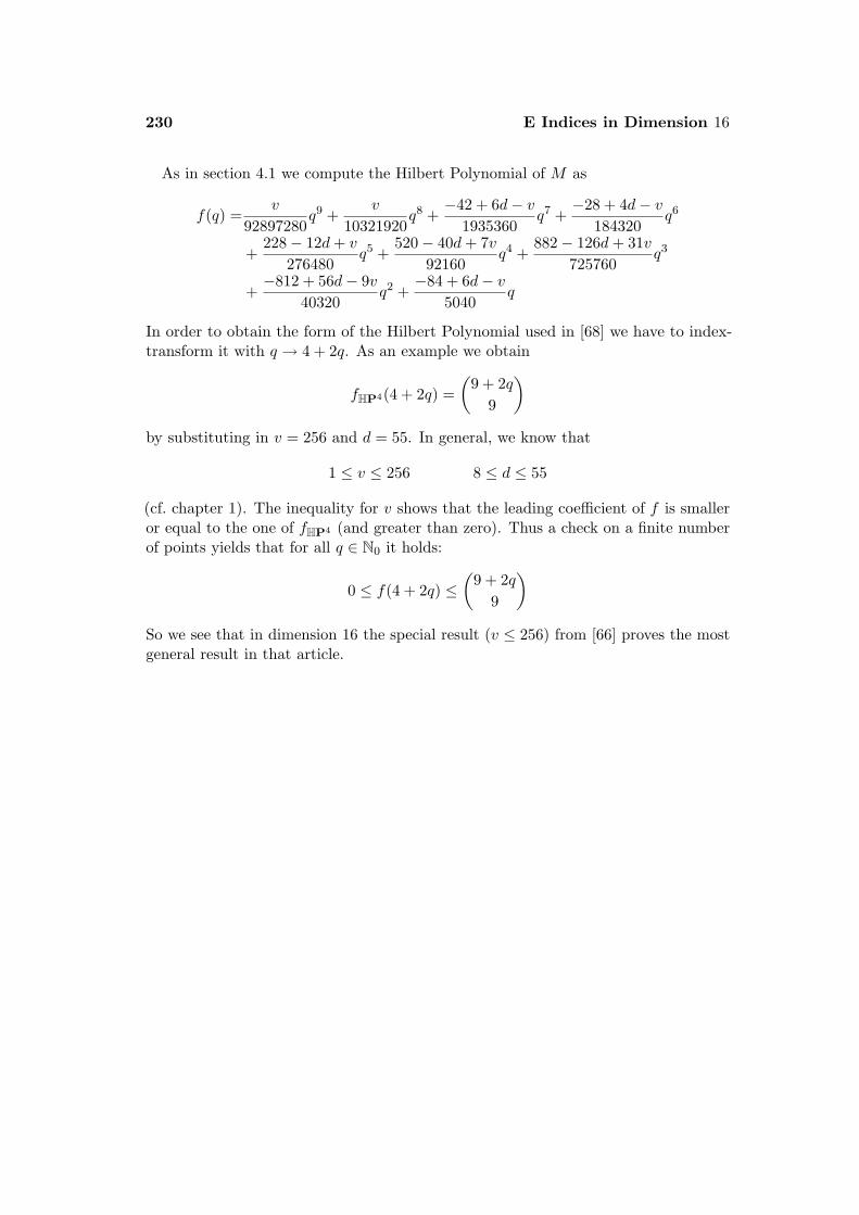
230 E Indices in Dimension 16
As in section 4.1 we compute the Hilbert Polynomial of M as
f(q) =v
92897280q9 +
v
10321920q8 +
−42 + 6d− v1935360
q7 +−28 + 4d− v
184320q6
+228− 12d+ v
276480q5 +
520− 40d+ 7v92160
q4 +882− 126d+ 31v
725760q3
+−812 + 56d− 9v
40320q2 +
−84 + 6d− v5040
q
In order to obtain the form of the Hilbert Polynomial used in [68] we have to index-transform it with q → 4 + 2q. As an example we obtain
fHP4(4 + 2q) =(
9 + 2q9
)by substituting in v = 256 and d = 55. In general, we know that
1 ≤ v ≤ 256 8 ≤ d ≤ 55
(cf. chapter 1). The inequality for v shows that the leading coefficient of f is smalleror equal to the one of fHP4 (and greater than zero). Thus a check on a finite numberof points yields that for all q ∈ N0 it holds:
0 ≤ f(4 + 2q) ≤(
9 + 2q9
)So we see that in dimension 16 the special result (v ≤ 256) from [66] proves the mostgeneral result in that article.
Bibliography
[1] C. Allday, V. Puppe, Cohomological Methods in Transformation Groups,Cambridge Studies in Advanced Mathematics 32, Cambridge University Press,1993
[2] M. Amann, A. Dessai, A note on the A-genus for π2-finite manifolds withS1-symmetry, arXiv:0811.0840v1, 2008
[3] M. F. Atiyah and F. Hirzebruch, Spin-manifolds and group actions, in: Essayson Topology and Related Topics (Memoires dedies a Georges de Rham),Springer, 1970, 18–28
[4] I. Belegradek, V. Kapovitch, Obstructions to nonnegative curvature andrational homotopy theory, Journal of the American Mathematical Society,Volume 15, Number 2, 2002, 259–284
[5] A. L. Besse, Einstein Manifolds, Springer, 2002
[6] R. Body, R. Douglas, Rational homotopy and unique factorization, PacificJournal of Mathematics, Volume 75, no. 2, 1978
[7] A. Borel, F. Hirzebruch, Characteristic classes and homogeneous spaces, II,Amer. J. Math. 81, 1959, 315–382
[8] A. Borel, J. de Siebenthal, Les sous-groupes fermes de rang maximum desgroupes de Lie clos, Commentarii Mathematici Helvetici 23, 1949
[9] R. Bott, C. Taubes, On the rigidity theorems of Witten, J. Amer. Math. Soc. 2,1989, 137–186
[10] G. E. Bredon, Introduction to Compact Transformation Groups, AcademicPress Inc., 1972
232 Bibliography
[11] Th. Brocker, T. tom Dieck, Representations of Compact Lie Groups, Springer,1985
[12] W. Browder, Surgery on simply connected manifolds, Springer, 1972
[13] G. R. Cavalcanti, New aspects of the ddc-lemma, PhD thesis,arXiv:math/0501406v1, January 2005
[14] G. R. Cavalcanti, The Lefschetz property, formality and blowing up in sym-plectic geometry, Transactions of the American Mathematical Society, Volume359, Number 1, 2007, 333–348
[15] A. Dancer, A. Swann, The Geometry of Singular Quaternionic Kahler Quo-tients, International Journal of Mathematics, Volume 8, no. 5, 1997, 595–610
[16] A. Dancer, A. Swann, Quaternionic Kahler manifolds of cohomogeneity one,International Journal of Mathematics, Volume 10, no. 5, 1999, 541–570
[17] P. Deligne, P. Griffiths, J. Morgan, D. Sullivan, Real Homotopy Theory ofKahler Manifolds, Inventiones Mathematicae 29, 1975, 245–274
[18] M. P. do Carmo, Riemannian Geometry, Birkhauser Boston, 1993
[19] F. Fang, Positive Quaternionic Kahler Manifolds and Symmetry Rank, Journalfur die reine und angewandte Mathematik, 2004, 149–165
[20] F. Fang, Positive Quaternionic Kahler Manifolds and Symmetry Rank: II,Math. Res. Lett. 15, no. 4, 2008, 641–651
[21] Y. Felix, St. Halperin, J.-C. Thomas, Elliptic spaces, Bulletin (new series) ofthe American Mathematical Society, Volume 25, Number 1, 1991
[22] Y. Felix, St. Halperin, J.-C. Thomas, Rational Homotopy Theory, Springer,2001
[23] M. Fernandez, V. Munoz, Formality of Donaldson submanifolds,arXiv:math.SG/0211017v2, October 2004
[24] M. Fernandez, V. Munoz, On non-formal simply connected manifolds,arXiv:math/0212141v3, January 2003
[25] M. Fernandez, V. Munoz, J. A. Santisteban, Cohomologically Kahler manifoldswith no Kahler metric, arXiv:math/0212141v3, January 2002
[26] M. Fernandez, V. Munoz, Non-formal compact manifolds with small Bettinumbers, arXiv:math/0504396v2, May 2006
Bibliography 233
[27] A. Fujiki, On the de Rham cohomology group of a compact Kahler symplecticmanifold, Algebraic geometry, Sendai, 1985, Adv. Stud. Pure Math., 10,North-Holland, Amsterdam, 1987, 105–165
[28] K. Galicki, S. Salamon, Betti Numbers of 3-Sasakian Manifolds, GeometriaeDedicata 63, 1996, 45–68
[29] A. Garvın, L. Lechuga, The computation of the Betti numbers of an ellipticspace is a NP-hard problem, Topology and its Applications, Volume 131, Issue3, 2003, 235–238
[30] A. Gray, A note on manifolds whose holonomy is a subgroup of Sp(n)Sp(1),Mich. Math. J. 16, 1965, 125–128
[31] W. Greub, St. Halperin, R. Vanstone, Connections, curvature and cohomology,Volume III, Academic Press, Inc., 1976
[32] P. Griffiths, J. Harris, Principles of Algebraic Geometry, John Wiley & Sons,Inc., 1978
[33] K. Grove, St. Halperin, Dupin hypersurfaces, group actions and the doublemapping cylinder, Journal of Differential Geometry 26, 1987, 429–459
[34] St. Halperin, Finiteness in the minimal models of Sullivan, Trans. Amer. Math.Soc. 230, 1977, 173–199
[35] H. Herrera, R. Herrera, A-genus on non-spin manifolds with S1 actionsand the classification of positive quaternion-Kahler 12-manifolds, Journalof Differential Geometry 61, 2002, 341–364
[36] H. Herrera, R. Herrera, Elliptic genera on non-spin Riemannian symmetricspaces with b2 = 0, Journal of Geometry and Physics 49, 2004, 197–205
[37] H. Herrera, R. Herrera, The signature and the elliptic genus of π2-finitemanifolds with circle actions, Topology and its Applications 136, 2004, 251–259
[38] R. Herrera, Positive Quaternion-Kahler 16-Manifolds with b2 = 0,Quart. J. Math. 57, no. 2, 2006, 203–214
[39] F. Hirzebruch and P. Slodowy, Elliptic genera, involutions, and homogeneousspin manifolds, Geometriae Dedicata 35, 1990, 309–343
[40] F. Hirzebruch, Th. Berger, R. Jung, Manifolds and Modular forms,Friedr. Vieweg & Sohn Verlagsgesellschaft, 1992
[41] D. D. Joyce, Compact manifolds with special holonomy, Oxford UniversityPress, Oxford Mathematical Monographs, Oxford, 2000
234 Bibliography
[42] V. Kapovitch, A note on rational homotopy of biquotients, preprint
[43] J. H. Kim, Rigidity theorems for positively curved manifolds with symmetry,Israel J. Math., to appear
[44] J. H. Kim, On positive quaternionic Kahler manifolds with b4 = 1, 2008
[45] S. Kobayashi, K. Nomizu, Foundations of differential geometry Volume I,John Wiley & Sons, 1996
[46] S. Kobayashi, K. Nomizu, Foundations of differential geometry Volume II,John Wiley & Sons, 1996
[47] R. Kobayashi, Ricci Flow unstable cell centered at an Einstein metric onthe twistor space of positive quaternion Kahler manifolds of dimension ≥ 8,arXiv:0801.2605v7 [math.DG], October 2008
[48] A. Kollross, A Classification of Hyperpolar and Cohomogeneity One Actions,Dissertation, Shaker, 1998
[49] D. Kotschick, On products of harmonic forms, Duke Mathematical Journal,Volume 107, No. 3, 2001
[50] D. Kotschick, S. Terzic, On formality of generalized symmetric spaces,Math. Proc. Camb. Phil. Soc. 134, 2003, 491–505
[51] D. Kotschick, S. Terzic, Geometric formality of Homogeneous Spaces andBiquotients, arXiv.0901.2267v1, 2009
[52] H. B. Lawson, M.-L. Michelsohn, Spin Geometry Princeton University Press,1994
[53] C. LeBrun, Fano manifolds, contact structures and quaternionic geometry,Int. J. Maths. 3, 1995, 353–376
[54] C. LeBrun, Simon Salamon, Strong rigidity of positive quaternion Kahlermanifolds, Inventiones Mathematicae 118, 1994, 109–132
[55] St. Lillywhite, Formality in an equivariant setting, Transactions of the Ameri-can Mathematical Society, Volume 355, Number 7, 2003, 2771–2793
[56] G. Lupton, Variations on a conjecture of Halperin, arXiv:math.AT/0010124,October 2000
[57] M. Mimura, H. Toda, Topology of Lie Groups, I and II, Kinokuniya CompanyLtd. Publishers, Tokyo, 1978
[58] W. Meier, Rational Universal Fibrations and Flag Manifolds, Math. Ann. 258,1983, 329–340
Bibliography 235
[59] W. Meier, Some topological properties of Kahler manifolds and homogeneousspaces, Math. Z. 183, 1983, 473–481
[60] S. A. Merkulov, Formality of canonical symplectic complexes and Frobeniusmanifolds Internat. Math. Res. Notices, 14, 1998, 727–733
[61] T. Nagano, M. Takeuchi, Signature of Quaternionic Kaehler Manifolds,Proc. Japan. Acad. 59 Ser. A, 1983, 384–386
[62] P.-A. Nagy, On length and product of harmonic forms in Kahler geometry,arXiv:math/0406341v2, June 2005
[63] J. Neisendorfer and T. J. Miller, Formal and coformal spaces, Illi-nois. J. Math. 22, 1978, 565–580
[64] A. L. Onishchik, Topology of Transitive Transformation Groups, JohannAmbrosius Barth, Leipzig, 1994
[65] S. Salamon, Index Theory and Quaternionic Kahler Manifolds, DifferentialGeometry and its Applications, Proc. Conf. Opava, August 24–28, 1992,Silesian University, Opava, 1993, 387–404
[66] S. Salamon, Quaternionic Kahler Manifolds, Inventiones Mathematicae 67,1982, 143–171
[67] S. Salamon, Quaternionic Kahler Geometry, Proceedings of the University ofCambridge VI, 1999, 83–121
[68] U. Semmelmann, G. Weingart, An upper bound for a Hilbert polynomial onquaternionic Kahler manifolds, arXiv:math.DH/0208079v1, August 2002
[69] H. Shiga, M. Tezuka, Rational Fibrations, Homogeneous Spaces with positiveEuler Characteristic and Jacobians, Ann. Inst. Fourier, Grenoble 37, no. 1,1987, 81–106
[70] W. Singhof, On the topology of double coset manifolds, Math. Ann. 297, 1993,133–146
[71] Z. Stepien, On formality of a class of compact homogeneous spaces, GeometriaeDedicata 93, 2002, 37–45
[72] D. Sullivan, Infinitesimal computations in topology, PublicationsMathematiques de l’IHES, no. 47, 1977, 269–331
[73] H. Tasaki, Quaternionic submanifolds in quaternionic symmetric spaces,Tohoku Math. Journ., 38, 1986, 513–538
236 Bibliography
[74] A. Tralle, On compact Homogeneous Spaces with non-vanishing Masseyproducts, Differential Geometry and its Applications, Proc. Conf. Opava,1993, 47–50
[75] R. O. Wells, Differential Analysis on Complex Manifolds, Springer, 1980
[76] B. Wilking, Torus actions on manifolds of positive sectional curvature, ActaMath. 191, 2003, 259–297
Notation Index
', 23, 24'Q, 23⊗, 19, 24, 39t, 53
(A, 0), 27, 29(A, d), 24ADR(M), 23, 29APL(M), 23, 24, 29A(M), 17, 131, 224A(M)[M ], iii, v, vi, 45, 51, 129, 136,
145, 152, 160, 199, 211
BG, 25bi, iv, 7, 10, 11, 22, 118, 144, 179
C, 37Ci, 37ci, 9, 22, 135, 142–144c0, 84, 126χ(M), v, 148, 185, 187, 193, 199, 207,
208, 229χπ(M), 41cat0, 41, 84, 126CG(H), 165, 166ch(E), 130cl0, 84
d, 18, 129, 145, 150, 166
d, 24D/, 17D/(E), 17, 172
E, 9∧k0 E, 17, 18
e0, 84ε, 10, 11, 16End(TM), 8
F0, 43, 44, 71, 72, 85FS1(M), 185, 197FZ2(M), 193, 198f , 38f∗, 38
G2, iv, 4, 118, 119, 122G2/SO(4), 174, 178, 179, 202G/H, iv, 25, 26, 38, 93, 98, 102, 107–
109, 220GH, 26, 44, 96, 112Gr2(Cn+2), 7, 10, 18, 173, 175, 177,
179, 181, 183, 188, 195Gr4(Rn+4), iii, 7, 45, 46, 49, 143, 146,
157, 161, 173, 174, 177, 179,181, 184, 190, 211, 212, 214,219
H, 7, 9
238 Notation Index
H∗(M), 25, 28, 41, 57H2(M), 83H2(M,R), 10H2(M,Z), 11Hk
(∧V,d
), 43
H i(M), 9, 12, 23, 29, 173H∗0 (M), 14Hol(M, g), 2HPn, ii, iv, vi, 6–8, 10, 18, 22, 142, 144,
148, 151, 173, 182, 188, 211,212, 230
hur, 28hur∗, 29
I(N), 36ip,q, 17, 18, 21, 129, 132, 133, 137, 148,
161, 162, 172, 224–227IrrC, 19IrrH, 19IrrR, 19Is, 37Isom(M), iv, v, 18, 20, 129, 145, 150,
166, 171, 172Isom0(M), 19, 150, 157, 160, 188
K, 28
L(M), 17, 227L(M)[M ], 16, 137l, 11
N , 37N i, 37∇, 2∇g, 2
PC(H), 7π2(M), iii, 10, 12, 46, 52, 199, 211πi(M), 28, 96, 100πi(φ), 23πi(M)⊗Q, 23, 28, 42, 56, 126πi(Sn)⊗Q, 22, 30Φ(M), 53, 152, 211, 215, 218Φ(M, g), 53, 215, 219, 221
ϕ, 20, 200, 204, 208
SlH, 17, 18scal(p), 5, 6sign(M), 13, 152, 211, 214, 227Sp(n), 4, 6, 19, 20Sp(n)Sp(1), 4–8, 11, 20, 196Spin(7), iv, 4, 118, 119, 122
TC(M), 9, 129, 152, 215
u, 9, 12, 22, 143, 144
v, 9, 145, 150, 152V k, 25V ≤k, 25∧V , 24(∧V,d
), 24∧k V , 25
W(G), 44, 176–178, 212, 221
Z, 7–13, 33, 83z, 11
Index
Betti number, iv, 7, 10, 11, 22, 118, 144,179
homotopy, 127biquotient, 26, 42–44, 55, 112, 114
formal, 44, 96, 112
cochain algebra, 24, 27cohomology, 9
primitive, 14rational, v, 29, 56, 84, 173, 199
commutative differential graded algebra,23
formal, 27, 29, 30, 37, 39complex structure, 6, 7, 33, 117conjecture
Bott, 42, 85Halperin, 71, 109, 113, 114LeBrun–Salamon, i, ii, iv, 6, 7, 21,
45, 53, 162connection, 1
Levi–Civita, 2curvature
Ricci, 5scalar, 5, 6, 45, 85sectional, 5, 6, 21, 42, 108
decomposable element, 32Dirac operator, 17
index of, 17
twisted, 17index of, 17, 172
equivalencerational homotopy, 23weak, 24, 29, 33
Euler characteristic, ii, v, 44, 120, 148,179, 185, 187, 193, 199, 200,207, 208, 229
homotopy, 41
fibrationmodel of, 25, 31non-primitive, 32, 58, 89, 91, 92primitive, 32, 55, 58, 90, 116spherical, ii, iii, 30–32, 57, 72, 76,
80, 82, 86, 87, 91–93totally non-cohomologous to zero,
32, 72, 87, 113twistor, iii, 7, 8, 12, 14, 56, 83, 85,
229finite type, 24fixed-point component, ii, iii, 20, 21, 47,
50, 161, 181, 185, 193, 197, 198,200, 201, 215
formalbiquotient, see biquotient, formalcommutative differential graded al-
gebra, see commutative differ-
240 Index
ential graded algebra, formaldimension, 41, 118manifold, see manifold, formalmap, iii, 38, 39, 76, 80, 81, 83, 85root, 130, 216
equivariant, 215space, see space, formalSullivan algebra, see Sullivan alge-
bra, formalSullivan model, see Sullivan model,
formal
genus, 16A-, iii, v, vi, 17, 45, 51, 129, 131,
136, 145, 152, 160, 199, 211,224
elliptic, ii, v, 16, 17, 46, 53, 152,211, 215, 218
equivariant, 53, 211, 217, 219L-, 16, 17, 137, 227
geometric formality, 86group
actioncohomogeneity one, 42, 158, 160isometric, 181transitive, 158, 160, 169, 181
isometry, iv, v, 18–20, 129, 145, 150,157, 160, 166, 171, 172, 188
Lie, 18, 19, 26, 42, 53, 96, 98, 99,129, 153, 167, 172
Weyl, 44, 176–178, 212, 221
Hard-Lefschetz property, 12, 113, 114,116–118
holonomy group, 2, 4of S2, 3
homology, 10, 11, 25, 28, 41, 57, 83Hurewicz homomorphism, 28
rationalised, 29, 57, 71, 80, 82, 102
intersection form, 13, 147, 228, 229
lemmaconnectivity, 19
ddc-, 33Hirsch, 12, 32, 82, 88surgery, 51
lower grading, 43, 115, 116
manifold3-Sasakian, 8, 87, 108Calabi–Yau, i, 4cohomologically symplectic, 116
quaternionic, 117Einstein, 6equivariantly bordant, 52Fano contact, i, 9, 10formal, ii–iv, 37, 55, 83–85, 88, 91,
109, 116, 117, 120, 122, 123,125
G2-, 4, 118elliptic, iv, 119, 122
homothetic, 10hyperKahler, 4, 6, 7Joyce, i, ii, 55, 113Kahler, 4, 6, 9, 10, 14, 20, 32, 33,
100, 103, 113, 117Non-Negative Quaternion Kahler,
85non-spin, 46π2-finite, 12Positive Quaternion Kahler, i–v, 1,
6, 7, 9–11, 13, 16, 18, 21, 45,53, 56, 83, 113, 123, 127, 142,144, 146, 148, 150, 157, 166,172, 207, 208
elliptic, iv, 122, 127formal, ii, iii, 55, 83, 84, 122, 123,
125Quaternion Kahler, 4–6, 8, 85rationally 3-connected, 12(rationally) elliptic, ii, 85, 112, 118,
119, 122spin, 16, 17, 45, 53, 118, 211Spin(7)-, 4, 118
elliptic, iv, 119, 122symplectic, 33, 116, 117
Index 241
totally geodesic, 20
parallel transport, 1, 3product
Kronecker, 19Massey, 33tensor, 19, 24, 39
quasi-isomorphism, 24, 29, 33, 35, 36,59
quaternionic volume, 9, 145, 150, 152
rationalcup-length, 84, 126dichotomy, 41, 126Lusternik–Schnirelmann category,
41, 84, 126rational homotopy
equivalence, 23, 24groups, 28, 42, 56, 96, 100, 126
of spheres, 22, 30theory, iii, 22, 29type, 23, 24, 29, 30, 84, 119
rationalisation, 23representation
complex, 49real, 49
spaceF0-, 43, 44, 71, 72, 85formal, ii–iv, 29, 33, 36, 37, 39, 43,
44, 55, 57, 71, 72, 80–86, 88–91,100, 112, 114, 116, 117, 120,122, 123, 125
example of, 30, 32, 99s-formal, 37, 123H-, 26, 32, 37, 39, 42homogeneous, iv, 6, 25, 26, 38, 43,
92, 93, 97, 98, 102, 103, 107,109, 114, 118, 181, 220
formal, 38, 98, 108non-formal, ii, iv, 92, 103, 108,
109, 112n-connected, 28
π2-finite, iii, 10, 12, 46, 52, 199, 211rationally 3-connected, iii, 10, 12,
199, 211(rationally) elliptic, ii, iv, 41–43, 55,
85, 92, 95, 100, 102, 109, 112,115, 118, 119, 122, 127
example of, 42positively, 115, see space, F0-
(rationally) hyperbolic, 41rationally n-connected, 28simply-connected, 4, 6, 9, 10, 23symmetric, ii, v, 4, 6, 8, 32, 45, 84,
127, 142, 152, 161, 172, 173,179, 181, 197–199, 211
N -symmetric, 32, 86twistor, 7–10, 12, 13, 84Wolf, ii, iv, v, 6, 8, 45, 84, 127, 142,
161, 173, 179, 181, 197, 198,211
spatial realisation, 24Sullivan
algebraformal, 35, 36, 114minimal, 24, 27, 35, 36, 58, 59,
89, 90, 114, 115pure, 43, 114, 115
model, 24–26formal, 35, 36, 120s-formal, 37minimal, 24–28, 30, 33, 35, 36,
58, 59, 66, 93, 95pure, 43, 44, 92, 113, 114, 116,
117representative, 38
tensorcurvature, 5metric, 6Ricci, 5, 6
theoremAtiyah–Singer Index, 17Berger, 4Bott–Taubes, 46
242 Index
Bredon, 49, 53cohomological properties, 11finiteness, 7Herrera–Herrera, 45Hirzebruch–Slodowy, 46Hurewicz, 11, 80Kodaira vanishing, 10Lefschetz fixed-point, 48, 169Myers, 10strong rigidity, 10
theoryindex, iii, v, 16, 129, 212irritations with, 21, 45, 152Lie, vrational homotopy, iii, see rational
homotopy, theorysurgery, 51, 109twistor, 10
transgression, 32, 56, 99
. . .And on the pedestal these words appear:“My name is Ozymandias, king of kings:Look on my works, ye Mighty, and despair!”Nothing beside remains: Round the decayOf that colossal wreck, boundless and bare,The lone and level sands stretch far away.
Percy Bysshe Shelley, “Ozymandias”


