practical aspects for designing statistically optimal ... · practical aspects for designing...
TRANSCRIPT

1 NDIA 2012 Practical Aspects
Optimal Experiments
Practical Aspects for Designing
Statistically Optimal Experiments
from an engineer’s perspective
Mark J. Anderson, PE
Stat-Ease, Inc.
Pat Whitcomb
Stat-Ease, Inc.

Agenda
What’s required for a good design.
Optimal point selection (IV versus D optimality).
Practical aspects algorithmic design.
Optimal design example.
Conclusion and recommendations.
2 NDIA 2012 Practical Aspects
Optimal Experiments
Study Considerations An Experimenter’s (Practical) View
What is the objective of the study?
State the objective in terms of measured
responses:
How will the responses be measured?
What precision is required?
Which factors will be studied?
What are the regions of interest and operability?
How will the response behave—linear or curvy?
What design should we use?
3 NDIA 2012 Practical Aspects
Optimal Experiments
“Good” Response Surface Designs A Statistician’s Checklist
Allow the chosen polynomial to be estimated well.
Give sufficient information to allow a test for lack of fit.
Have more unique design points than coefficients in model.
Provide an estimate of “pure” error.
Be insensitive (robust) to the presence of outliers in the data.
Be robust to errors in control of the factor levels.
Permit blocking and sequential experimentation.
Provide a check on homogeneous variance assumption and
other useful model diagnostics; including deletion statistics.
Generate useful information throughout the region of interest,
i.e., provide a good distribution of standard error of prediction.
Not contain an excessively large number of runs.
4 NDIA 2012 Practical Aspects
Optimal Experiments

“Good” Response Surface Designs Comments on the Checklist
Re: Pitfalls of Optimality:
“Souped-Up Car Syndrome:
Optimize speed and produce a delicate gas-guzzler.”
Peter J. Huber*
“Designing an experiment should involve balancing multiple
objectives, not just focusing on a single characteristic.”
Myers, Montgomery and Anderson-Cook**
“Alphabetic optimality is not enough!”
Pat Whitcomb
5 NDIA 2012 Practical Aspects
Optimal Experiments
* “On the Non-Optimality of Optimal Procedures” Optimality: Lehmann Symposium,
Institute of Mathematical Statistics, 2009, 31-46.
** Response Surface Methodology, 3rd Ed, Wiley, 2009.

Agenda
What’s required for a good design.
Optimal point selection (IV versus D optimality).
Practical aspects algorithmic design.
Optimal design example.
Conclusion and recommendations.
6 NDIA 2012 Practical Aspects
Optimal Experiments

Optimal Point Selection D-optimal Point Selection
Goal: D-optimal design minimizes the determinant of the (X'X)-1
matrix. This minimizes the volume of the confidence
ellipsoid for the coefficients and maximizes information
about the polynomial coefficients.
7
2
1
Correlated Coefficients
1
2
Uncorrelated Coefficients
NDIA 2012 Practical Aspects
Optimal Experiments
Optimal Point Selection IV-optimal Point Selection
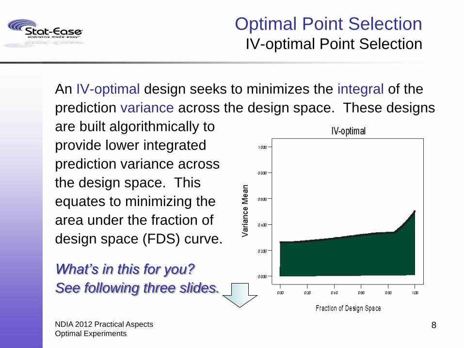
An IV-optimal design seeks to minimizes the integral of the
prediction variance across the design space. These designs
are built algorithmically to
provide lower integrated
prediction variance across
the design space. This
equates to minimizing the
area under the fraction of
design space (FDS) curve.
What’s in this for you?
See following three slides.
8 NDIA 2012 Practical Aspects
Optimal Experiments

Primer on FDS One Factor (part 1 of 2)
NDIA 2012 Practical Aspects
Optimal Experiments 9
Note: The actual precision of
the fitted value depends on
where we are predicting. 3
4
5
6
7
R1
One Factor Experiment
0 0.25 0.5 0.75 1 Factor A
y d
Solid center line is fitted model
is expected value (mean prediction)
Curves are confidence limits
(actual precision)
d is half-width of the desired CI
(desired precision)—it creates
the red lines.
y

Primer on FDS One Factor (part 2 of 2)
NDIA 2012 Practical Aspects
Optimal Experiments 10
Design-Expert® Software
Min Std Error Mean: 0.447Avg Std Error Mean: 0.532Max Std Error Mean: 0.671Cuboidalradius = 1Points = 50000t(0.05/2,3) = 3.18245d = 0.9, s = 0.55FDS = 0.51Std Error Mean = 0.514
FDS Graph
Fraction of Design Space
Std
Err
or
Mean
0.00 0.20 0.40 0.60 0.80 1.00
0.000
0.200
0.400
0.600
0.800
1.000
Only 51% of the design space
is precise enough to predict
the mean within 0.90.

Primer on FDS Two Factor
NDIA 2012 Practical Aspects
Optimal Experiments 11
Fraction of Design Space
0.00 0.25 0.50 0.75 1.00
0.000
0.200
0.400
0.600
0.800
1.000
Fraction of Design Space
0.63
0.51 0.46
50% 75% 95%

Optimal Point Selection IV versus D Optimal Design
Compare point selection using IV-optimal and D-optimal:
Build a one factor design.
Design for a quadratic model.
Choose 12 runs using optimality as the only criterion.
12 NDIA 2012 Practical Aspects
Optimal Experiments

IV versus D Optimal Design Optimal 12 Point Designs
13
-1.00 0.00 1.00
0.30
0.40
0.50
0.60
0.70
A: A
Std
Err o
f D
es
ign
D-optimal
4 4 4
-1.00 0.00 1.00
0.30
0.40
0.50
0.60
0.70
A: A
Std
Err o
f D
es
ign
IV-optimal
3
6
3
NDIA 2012 Practical Aspects
Optimal Experiments
Compare and contrast.

IV-optimal versus D-optimal One Factor 12 Optimal Points
14
Fraction of Design Space Graph S
tdE
rr M
ean
0.00 0.20 0.40 0.60 0.80 1.00
0.300
0.400
0.500
0.600
Fraction of Design Space
IV min: 0.382
IV avg: 0.421
IV max: 0.577
D min: 0.395
D avg: 0.447
D max: 0.500
NDIA 2012 Practical Aspects
Optimal Experiments
Compare and contrast.

What about G-Optimality? Three 6-Point 2-Factor Designs
G-optimal designs:
o Minimize the maximum predicted variance.
o This is at the expense of the average prediction variance.
o For a gain in a very small fraction of the design space,
precision is sacrificed in the vast majority of the design
space. (see next slide)
15
G-optimal D-optimal IV-optimal
G efficiency 87.9% 66.4% 56.5%
Min SE mean 0.653 0.604 0.566
Ave SE mean 0.777 0.743 0.699
Max SE mean 0.923 1.063 1.152
NDIA 2012 Practical Aspects
Optimal Experiments

What about G-Optimality? Three 6-Point 2-Factor Designs
NDIA 2012 Practical Aspects
Optimal Experiments 16
Fraction of Design Space
Std
Err
or
Mean
0.00 0.20 0.40 0.60 0.80 1.00
0.50
0.60
0.70
0.80
0.90
1.00
1.10
1.20
G is an unhappy compromise.

Optimal Point Selection IV versus D Optimal Design
Conclusions:
IV-optimal designs tend to place points more uniformly
in the design space.
IV-optimal designs have a higher maximum prediction
variance; therefore a lower G-efficiency.
IV-optimal designs have a lower average prediction
variance. (This also contributes to a lower G-efficiency.)
Being minimum level designs neither IV nor D can
evaluate sufficiency of quadratic model! They
must be augmented to test lack of fit.
17 NDIA 2012 Practical Aspects
Optimal Experiments

Agenda
What’s required for a good design.
Optimal point selection (IV versus D optimality).
Practical aspects algorithmic design.
Optimal design example.
Conclusion and recommendations.
18 NDIA 2012 Practical Aspects
Optimal Experiments

Optimal Point Selection IV versus D Optimal Design
Compare point selection using IV-optimal and D-optimal :
Build a one-factor design.
Design for a quadratic model.
Choose eight of the twelve runs using optimality as
the criteria.
Choose four of the twelve runs as lack of fit (LOF)
points using distance as the criteria. (Maximize the minimum distance from an existing design
point; i.e. fill the “holes”.)
19 NDIA 2012 Practical Aspects
Optimal Experiments

Optimal Designs 8 Optimal + 4 LOF Points
20
-1.00 -0.67 -0.33 0.00 0.33 0.67 1.00
0.30
0.40
0.50
0.60
0.70
A: A
Std
Err o
f D
es
ign
IV-optimal
2
4
2
-1.00 -0.67 -0.33 0.00 0.33 0.67 1.00
0.30
0.40
0.50
0.60
0.70
A: A
Std
Err o
f D
es
ign
D-optimal
3
2
3
NDIA 2012 Practical Aspects
Optimal Experiments

IV-optimal versus D-optimal One-Factor Design, 8 Optimal + 4 LOF Points
21
IV min: 0.381
IV avg: 0.438
IV max: 0.653
D min: 0.395
D avg: 0.448
D max: 0.547
NDIA 2012 Practical Aspects
Optimal Experiments
FDS Graph
Fraction of Design Space
Std
Err
Me
an
0.00 0.20 0.40 0.60 0.80 1.00
0.300
0.400
0.500
0.600
0.700
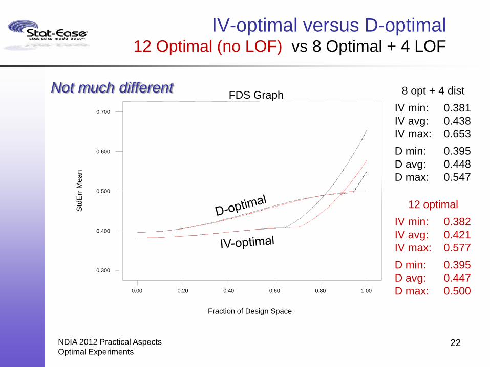
IV-optimal versus D-optimal 12 Optimal (no LOF) vs 8 Optimal + 4 LOF
22
8 opt + 4 dist
IV min: 0.381
IV avg: 0.438
IV max: 0.653
D min: 0.395
D avg: 0.448
D max: 0.547
12 optimal
IV min: 0.382
IV avg: 0.421
IV max: 0.577
D min: 0.395
D avg: 0.447
D max: 0.500
NDIA 2012 Practical Aspects
Optimal Experiments
FDS Graph
Fraction of Design Space
Std
Err
Me
an
0.00 0.20 0.40 0.60 0.80 1.00
0.300
0.400
0.500
0.600
0.700
Not much different

Optimal Point Selection IV versus D Optimal Design
Compare point selection for a two-factor 14-run design:
Design for a quadratic model.
IV-optimal:
14 optimal runs (no LOF)
10 optimal and 4 LOF (distance)
D-optimal:
14 optimal runs (no LOF)
10 optimal and 4 LOF (distance)
23 NDIA 2012 Practical Aspects
Optimal Experiments

IV-optimal Designs 14-Run Designs with 0 vs 4 LOF Points
24
-1.00 -0.50 0.00 0.50 1.00
-1.00
-0.50
0.00
0.50
1.0010 IV-optimal and 4 LOF
0.500
0.6000.700 0.700
0.700 0.700
0.800 0.800
2
-1.00 -0.50 0.00 0.50 1.00
-1.00
-0.50
0.00
0.50
1.0014 IV-optimal
0.5000.600
0.600
0.700
0.700
0.7000.700
0.800
0.800
2
2
4
NDIA 2012 Practical Aspects
Optimal Experiments
Std
Err
or
of D
esig
n

IV-optimal Designs 14-Run Designs with 0 vs 4 LOF Points
NDIA 2012 Practical Aspects
Optimal Experiments 25
FDS Graph
Fraction of Design Space
Std
Err
or
Me
an
0.00 0.20 0.40 0.60 0.80 1.00
0.000
0.200
0.400
0.600
0.800
1.000
14 IV-optimal points
IV min: 0.418
IV avg: 0.515
IV max: 0.908
10 IV-optimal + 4 LOF points
IV min: 0.435
IV avg: 0.528
IV max: 0.857
Not much difference

D-optimal Designs 14-Run Designs with 0 vs 4 LOF Points
26
-1.00 -0.50 0.00 0.50 1.00
-1.00
-0.50
0.00
0.50
1.0010 D-optimal and 4 LOF
0.50
0.60
0.70 0.70
0.70
0.80
2
-1.00 -0.50 0.00 0.50 1.00
-1.00
-0.50
0.00
0.50
1.0014 D-optimal
0.50 0.50
0.500.50
0.600.60
0.60
0.60 0.60
0.60
2 2
2
2 2
NDIA 2012 Practical Aspects
Optimal Experiments
Std
Err
or
of D
esig
n
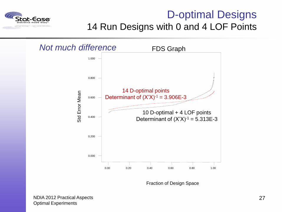
D-optimal Designs 14 Run Designs with 0 and 4 LOF Points
NDIA 2012 Practical Aspects
Optimal Experiments 27
FDS Graph
Fraction of Design Space
Std
Err
or
Me
an
0.00 0.20 0.40 0.60 0.80 1.00
0.000
0.200
0.400
0.600
0.800
1.000
14 D-optimal points
Determinant of (X’X)-1 = 3.906E-3
10 D-optimal + 4 LOF points
Determinant of (X’X)-1 = 5.313E-3
Not much difference

Practical Aspects Algorithmic Design Lack of Fit Points
Adding LOF points:
The design is not as alphabetically optimal but only
slightly off-kilter on FDS plot (not much difference).
Ability to detect lack of fit is enhanced.
Adding LOF points is a good trade off!
28 NDIA 2012 Practical Aspects
Optimal Experiments
Practical Aspects Algorithmic Design Pure Error Estimation
Estimating pure error:
In physical experiments it is desirable build in an
estimate of experimental error—just so you know.
Replicates provide an estimate of experimental error
independent of model assumptions. They allow for a
test on lack of fit.
Adding replicates is a good tradeoff!
29 NDIA 2012 Practical Aspects
Optimal Experiments

Agenda
What’s required for a good design.
Optimal point selection (IV versus D optimality).
Practical aspects algorithmic design.
Optimal design example.
Conclusion and recommendations.
30 NDIA 2012 Practical Aspects
Optimal Experiments
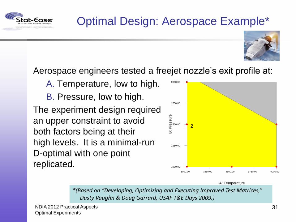
Optimal Design: Aerospace Example*
Aerospace engineers tested a freejet nozzle’s exit profile at:
A. Temperature, low to high.
B. Pressure, low to high.
The experiment design required
an upper constraint to avoid
both factors being at their
high levels. It is a minimal-run
D-optimal with one point
replicated.
NDIA 2012 Practical Aspects
Optimal Experiments 31
*(Based on “Developing, Optimizing and Executing Improved Test Matrices,” Dusty Vaughn & Doug Garrard, USAF T&E Days 2009.)
3000.00 3250.00 3500.00 3750.00 4000.00
1000.00
1250.00
1500.00
1750.00
2000.00
A: Temperature
B: P
ressu
re
2

This stouter design* features 4 more points for lack-of-fit
plus 4 points replicated for a stronger estimate of pure
error. Also, the optimality
criterion for this design is
IV—now favored for RSM
designs (vs the D-optimal
in vogue at the time of this
experiment).
Optimal Design: Aerospace Example An Alternative Design
NDIA 2012 Practical Aspects
Optimal Experiments 32
*(Detailed in “How to Frame a Robust Sweet Spot via Response Surface Methods”, 2010 NDIA T&E Conf talk by MJA.)

Design-Expert® Software
Min Std Error Mean: 0.409Avg Std Error Mean: 0.528Max Std Error Mean: 0.967ConstrainedPoints = 50000t(0.05/2,8) = 2.306d = 30, s = 20FDS = 0.91Std Error Mean = 0.650
FDS Graph
Fraction of Design Space
Std
Err
or
Me
an
0.00 0.20 0.40 0.60 0.80 1.00
0.000
0.200
0.400
0.600
0.800
1.000
Aerospace Example Evaluate your IV-optimal Design
Is the stouter optimal design precise enough?
Assume standard deviation of 20 for the prime response.
Then a difference “d” of 30 will likely be detected.*
*(Versus ~260 for the near-minimal D-optimal design!)
33 NDIA 2012 Practical Aspects
Optimal Experiments

Results*
NDIA 2012 Practical Aspects
Optimal Experiments 34
1000.00
1250.00
1500.00
1750.00
2000.00
3000.00
3250.00
3500.00
3750.00
4000.00
1000
1200
1400
1600
1800
2000
2200
Q
A: Temperature B: Pressure
1000.00
1250.00
1500.00
1750.00
2000.00
3000.00
3250.00
3500.00
3750.00
4000.00
400
500
600
700
800
900
1000
H
ts
A: Temperature B: Pressure
*(Generated via re-simulation from predictive equations provided in coded form by the experimenters. The graphs closely
resemble the published results for the key measures of dynamic pressure (Q) and total sensible enthalpy (Hts).)

Agenda
What’s required for a good design.
Optimal point selection (IV versus D optimality).
Practical aspects algorithmic design.
Optimal design example.
Conclusion and recommendations.
35 NDIA 2012 Practical Aspects
Optimal Experiments

Practical Aspects of DOE Remember what is Most Important
1. Identify opportunity and define objective.
2. State objective in terms of measurable responses.
Define the precision desired to predict each response.
Estimate experimental error ( ) for each response.
3. Select the input factors and ranges to study.
4. Select a design and:
Evaluate precision via the FDS plot.
Examine the design layout to ensure all the factor
combinations are safe to run and are likely to result in
meaningful information (no disasters).
36 NDIA 2012 Practical Aspects
Optimal Experiments

When Optimal Design is Necessary
Multiple linear constraints, such waffles made at right
temperature and time—not too little (runny!) and not
too much (burnt!)
Factors are categoric or discrete numeric
Models other than full quadratic handled by cataloged
RSM designs such as central composite
Always choose a design that fits the problem!
Size for precision!
37 NDIA 2012 Practical Aspects
Optimal Experiments

Practical Aspects Algorithmic Design Optimality Criteria
Should I use a D-optimal or IV-optimal design?
IV-optimal - precise estimation of the predictions
Best for empirical response surface design
D-optimal - precise estimation of model coefficients
Best for screening and mechanistic models
38 NDIA 2012 Practical Aspects
Optimal Experiments

Practical Aspects Algorithmic Design Suggestion for Point Selection
Given how many factors (k) you study and the number of
coefficients (p) in the model you select, use the following as
a guide to a starting design:
Model: p points using an optimality criteria
Lack-of-Fit: 5 points; based on distance or
estimating higher order model terms.
Replicates: 5 points, using the model optimality
criteria (most influential).
Evaluate precision of the starting design via the FDS plot:
If more precision is required, rebuild the design
adding more runs.
39 NDIA 2012 Practical Aspects
Optimal Experiments

Practical Aspects of DOE Keep in Mind
No alphabetic optimality or sophisticated statistical analysis
can make up for:
Studying the wrong problem.
Measuring the wrong response.
Not having adequate precision.
Testing the wrong factors.
Having too many runs outside the
region of operability.
40 NDIA 2012 Practical Aspects
Optimal Experiments

Thank you for your attention!
Practical Aspects for Designing
Statistically Optimal Experiments
from an engineer’s perspective
41
Mark Anderson, PE
Stat-Ease, Inc.
Pat Whitcomb
Stat-Ease, Inc.
NDIA 2012 Practical Aspects
Optimal Experiments