process analysis accelerator - holocentricdocuments.holocentric.com/public/hug/hug016 - process...
TRANSCRIPT
Process Analysis Accelerator
Version 6.0
User Guide
V1.0/HUG016

Process Analysis Accelerator User Guide
HUG016 – Process Analysis Accelerator 20 January 2012 Page 2 of 126 www.holocentric.com
Table of Contents
1 About this Guide ·························································································10
1.1 Conventions Used in This Manual ............................................................ 10
2 Process Analysis in Context ·········································································11
2.1 What is Business Process Analysis? .......................................................... 11
2.2 Why do Process Analysis? ........................................................................ 12
2.3 Which Processes Need Improvement?..................................................... 12
2.4 What is Path Analysis? ............................................................................. 14
3 Path Analysis in Holocentric Modeler ··························································15
3.1 Time Driven Activity Based Costing .......................................................... 16
3.2 Capacity Constraint Analysis .................................................................... 16
3.3 Concepts Defined ..................................................................................... 16
3.4 The Path Analysis Engine ......................................................................... 18
3.5 Simulation Prerequisites .......................................................................... 19
4 Using the Process Analysis Accelerator ························································20
4.1 Modeling with Process Analysis in Mind .................................................. 20
4.2 Developing and Defining the Process ....................................................... 20
4.3 Introducing the Actorless Swim Lane Notation ........................................ 20
4.3.1 Background ·········································································································· 20
4.3.2 Prerequisites ········································································································ 21
4.3.3 Directions ············································································································ 23
4.3.3.1 Creating a New Process Analysis library ················································· 23
4.3.3.2 Creating a New Process Diagram ···························································· 23
4.3.3.3 Creating and Placing Actors ···································································· 25
4.3.3.4 Reassigning Actors to Lanes ···································································· 25
4.3.3.5 Setting a Process Initiation Point ···························································· 25
4.3.3.6 Creating Process Steps ············································································ 26
4.3.3.7 Designating a Process Step as Decision Point ········································· 27
Process Analysis Accelerator User Guide
HUG016 – Process Analysis Accelerator 20 January 2012 Page 3 of 126 www.holocentric.com
4.3.3.8 Modeling a Sequence of Process Steps ·················································· 28
4.3.3.9 Modeling Actor Interactions ··································································· 28
4.3.3.10 Handing Off to Exit Processes ······························································· 29
4.3.3.11 Next Steps ····························································································· 29
4.4 Assigning Metrics to Process Elements .................................................... 30
4.4.1 Defining Activity Metrics ····················································································· 30
4.4.1.1 Background ····························································································· 30
4.4.1.2 Prerequisites ··························································································· 30
4.4.1.3 Directions ································································································ 30
4.4.1.4 Next Steps ······························································································· 34
4.4.2 Defining Role Metrics ·························································································· 34
4.4.2.1 Background ····························································································· 34
4.4.2.2 Prerequisites ··························································································· 35
4.4.2.3 Directions ································································································ 35
4.4.2.4 Next Steps ······························································································· 37
4.5 Exporting Metrics to Excel ....................................................................... 38
4.5.1 Background ·········································································································· 38
4.5.2 Prerequisites ········································································································ 38
4.5.3 Directions ············································································································ 38
4.5.4 Next Steps ··········································································································· 39
4.6 Editing Exported Metrics within Excel ...................................................... 39
4.6.1 Background ·········································································································· 39
4.6.2 Prerequisites ········································································································ 39
4.6.3 Directions ············································································································ 39
4.6.4 Results/Next Steps ······························································································ 42
4.7 Importing Updated Metrics from Excel .................................................... 42
4.7.1 Background ·········································································································· 42
4.7.2 Prerequisites ········································································································ 42
4.7.3 Directions ············································································································ 42
4.7.4 Results/Next Steps ······························································································ 43
4.8 Defining Process Constraints .................................................................... 44
Process Analysis Accelerator User Guide
HUG016 – Process Analysis Accelerator 20 January 2012 Page 4 of 126 www.holocentric.com
4.8.1 Setting Volume Constraints on Exchanges ·························································· 44
4.8.1.1 Background ····························································································· 44
4.8.1.2 Prerequisites ··························································································· 45
4.8.1.3 Directions ································································································ 45
4.8.1.4 Next Steps ······························································································· 47
4.8.2 Setting Resource Sharing Constraints on Interactions ········································ 47
4.8.2.1 Background ····························································································· 47
4.8.2.2 Prerequisites ··························································································· 48
4.8.2.3 Directions ································································································ 48
4.8.2.4 Next Steps ······························································································· 49
4.9 Running Process Simulation ..................................................................... 49
4.9.1 Defining the Scope of Analysis ············································································ 49
4.10 Setting a Start Point ............................................................................... 50
4.10.1 Background ·········································································································· 50
4.10.2 Prerequisites ········································································································ 50
4.10.3 Directions ············································································································ 50
4.10.4 Setting start point on the Initiating Actor node ·················································· 51
4.10.5 Setting Start Point on a Process Exchange ·························································· 51
4.10.6 Setting a Start Point on a Process Step ······························································· 52
4.10.7 Next Steps ··········································································································· 53
4.11 Setting an End Point ............................................................................... 53
4.11.1 Background ·········································································································· 53
4.11.2 Prerequisites ········································································································ 53
4.11.3 Directions ············································································································ 53
4.11.4 Setting an End Point on a Process Exchange ······················································· 54
4.11.5 Setting an End Point on a Process Step ······························································· 54
4.11.6 Next Steps ··········································································································· 55
5 Performing Path Analysis ············································································56
5.1 Set Excel Model Default Parameters ........................................................ 56
5.1.1 Background ·········································································································· 56
5.1.2 Prerequisites ········································································································ 57
Process Analysis Accelerator User Guide
HUG016 – Process Analysis Accelerator 20 January 2012 Page 5 of 126 www.holocentric.com
5.1.3 Directions ············································································································ 57
5.1.4 Next Steps ··········································································································· 58
5.2 Finding Paths ........................................................................................... 59
5.2.1 Background ·········································································································· 59
5.2.2 Prerequisites ········································································································ 59
5.2.3 Directions ············································································································ 60
5.2.4 Next Steps ··········································································································· 62
5.3 Launching the Excel Model Manually ....................................................... 62
5.3.1 Background ·········································································································· 62
5.3.2 Prerequisites ········································································································ 63
5.3.3 Directions ············································································································ 63
5.3.4 Next Steps ··········································································································· 66
5.4 Visualising Paths in Modeler .................................................................... 67
5.4.1 Assigning Labels to Paths in Excel ······································································· 67
5.4.1.1 Background ····························································································· 67
5.4.1.2 Prerequisites ··························································································· 67
5.4.1.3 Directions ································································································ 67
5.4.1.4 Next Steps ······························································································· 68
5.4.2 Showing Paths ····································································································· 69
5.4.2.1 Background ····························································································· 69
5.4.2.2 Prerequisites ··························································································· 69
5.4.3 Directions ············································································································ 69
5.4.4 Next Steps ··········································································································· 72
6 Constraining Path Analysis using Scenarios ·················································73
6.1 Defining Scenario Conditions ................................................................... 74
6.1.1 Background ·········································································································· 74
6.1.2 Prerequisites ········································································································ 76
6.1.3 Directions ············································································································ 77
6.1.4 Next Steps ··········································································································· 84
6.2 Finding Paths Using Scenarios .................................................................. 84
6.2.1 Background ·········································································································· 84
Process Analysis Accelerator User Guide
HUG016 – Process Analysis Accelerator 20 January 2012 Page 6 of 126 www.holocentric.com
6.2.2 Prerequisites ········································································································ 84
6.2.3 Directions ············································································································ 85
6.2.3.1 Create a New Path Options Definition ···················································· 85
6.2.3.2 Modify Path Options Settings ································································· 86
6.2.3.3 Process Simulation Using a Custom Path Options Definition ················· 87
6.2.4 Next Steps ··········································································································· 89
7 Appendix 1 - Process Analysis in Other Notations········································90
7.1 Background .............................................................................................. 90
7.2 Notation examples ................................................................................... 90
7.2.1 ‘Process Lane’ View with Actors Visible ······························································ 90
7.2.2 ‘Graph’ Process View ··························································································· 92
7.3 Setting Start and End Points ..................................................................... 93
7.3.1 Setting the Start Point ························································································· 93
7.3.2 Setting the End Point ··························································································· 94
7.3.3 Beyond Start and End Points ··············································································· 96
8 Appendix 2 - Using the Path Analysis Spreadsheet ······································97
8.1 Introducing the Excel Model .................................................................... 97
8.1.1 Discrete Process Execution Analysis (TDABC) ····················································· 99
8.1.2 Quick Indicators ································································································· 100
8.1.3 General Assumptions ························································································ 101
8.1.4 Constraint and Capacity Based Analysis ···························································· 101
8.1.5 Quick Indicators ································································································· 102
8.1.6 General Assumptions ························································································ 104
8.1.7 Exploring the Excel Model in Detail ·································································· 106
9 Dashboard Worksheet ·············································································· 107
9.1 Worksheet header ................................................................................. 107
9.2 Discrete Process Execution Model (Blue Headers) ................................. 108
9.3 Capacity Constraint Analysis Model (Yellow Headers) ........................... 111
9.4 Actors Worksheet .................................................................................. 112
9.5 RACI Worksheet ..................................................................................... 115
Process Analysis Accelerator User Guide
HUG016 – Process Analysis Accelerator 20 January 2012 Page 7 of 126 www.holocentric.com
9.6 Activities Worksheet .............................................................................. 116
9.7 Paths Worksheet .................................................................................... 121
9.8 FTE Weighted Average Utilization Worksheet ........................................ 124
9.8.1 Average Utilisation/Adjusted Average Utilisation Worksheets ························ 124
9.8.2 Workload/Adjusted Workload Worksheets ······················································ 124
9.8.3 Volumes/Adjusted Volumes Worksheets ························································· 124
10 Appendix 3 - XML Output File Schema and Format ···································· 125
10.1 XML Output File Schema ...................................................................... 125
10.2 XML Output File Example ..................................................................... 126
Process Analysis Accelerator User Guide
HUG016 – Process Analysis Accelerator 20 January 2012 Page 8 of 126 www.holocentric.com
Table of Figures
Figure 1 - A Sequence of Activities Linked by Notification Exchanges .......................................... 17
Figure 2 - Modeling the Hand-off to a Resultant Process Diagram .............................................. 18
Figure 3 - Actorless Swim Lane Process Diagram Notation .......................................................... 21
Figure 4 - Process Analysis Default Library ................................................................................... 23
Figure 5 - Actorless Swim Lane Toolbox ........................................................................................ 24
Figure 6 - Change Process Lane Orientation ................................................................................. 24
Figure 7 - Manually Adjust Pool Size ............................................................................................. 25
Figure 8 - Process Initiation Point ................................................................................................. 26
Figure 9 - IT Dependent Process Step ........................................................................................... 26
Figure 10 - Manual Process Step ................................................................................................... 27
Figure 11 - No Parent Defined ....................................................................................................... 27
Figure 12 - Flagged as a Decision .................................................................................................. 27
Figure 13 - Setting a Process Step as a Decision Point .................................................................. 28
Figure 14 - An Interaction as Represented in the Actorless Swim Lane Notation ........................ 29
Figure 15 - Exit Process Icon Showing Initiating Actor .................................................................. 29
Figure 16 - Process Step ‘Model’ Property Editor ......................................................................... 31
Figure 17 - Process Step ‘Appearance’ Property Editor ................................................................ 31
Figure 18 - Activity Metrics Data Entry Form ................................................................................ 32
Figure 19 - Show or Hide Activity Metrics on a Process Diagram ................................................. 34
Figure 20 - Actor ‘Model’ Property Editor ..................................................................................... 35
Figure 21 - Actor ‘Appearance’ Property Editor ............................................................................ 36
Figure 22 - Role Metrics Data Entry Form ..................................................................................... 36
Figure 23 - Choosing the Type of Item to Export to MS Excel®. .................................................... 38
Figure 24 - An example of the properties spreadsheet ................................................................ 41
Figure 25 - Property Import Confirmation Dialog ......................................................................... 43
Figure 26 - Read-only Items Not Updated .................................................................................... 43
Figure 27 - Percentage volume constraints on process exchanges .............................................. 45
Figure 28 - Process Exchange Property Dialog .............................................................................. 46
Figure 29 - A Process with Volume Constraints Defined .............................................................. 47
Figure 30 - An Interaction as Represented in the Actorless Swim Lane Notation ........................ 48
Figure 31 - Setting Constraints upon Interaction Exchanges ........................................................ 49
Figure 32 - Initiating Node ............................................................................................................. 50
Figure 33 - Start point set on an Initiating Actor node ................................................................. 51
Figure 34 - Setting the Start Point on an Exchange....................................................................... 51
Figure 36 - Setting the start point on a process step .................................................................... 52
Figure 35 - Start Point is Assigned to the Underlying Actor .......................................................... 52
Figure 37 - Setting an end point on a process exchange .............................................................. 54
Figure 38 - Setting an end point on a process step ....................................................................... 54
Figure 39 - End point with actor underlying actor shown ............................................................ 55
Figure 40 - Microsoft Security Notice ........................................................................................... 57
Figure 41 - Simulation Options dialog ........................................................................................... 58
Figure 42 - Find Paths dialog ......................................................................................................... 60
Figure 43 - Path Analysis Spreadsheet - Dashboard ..................................................................... 61
Figure 44 - Run Simulation Dialog Options ................................................................................... 64
Figure 45 - Set Path Label in Excel ................................................................................................. 67
Process Analysis Accelerator User Guide
HUG016 – Process Analysis Accelerator 20 January 2012 Page 9 of 126 www.holocentric.com
Figure 46 - Path label indicator ..................................................................................................... 68
Figure 47 - Mouse-over path label tool tip ................................................................................... 68
Figure 48 - Path Analysis Wizard – Page 1 .................................................................................... 70
Figure 49 - Path Analysis Wizard – Page 2 .................................................................................... 71
Figure 50 - Designation of shared paths ....................................................................................... 71
Figure 51 - An example of process divergence ............................................................................. 74
Figure 52 - Defining scenario conditions at a divergence ............................................................. 76
Figure 53 - Scenario Conditions Editor .......................................................................................... 77
Figure 54 - Adding a New Scenario ............................................................................................... 78
Figure 55 - Naming a scenario ....................................................................................................... 79
Figure 56 - Adding a Combination ................................................................................................. 80
Figure 57 - Defining a second Combination .................................................................................. 81
Figure 58 - Scenario Combination represented in real-time on the process diagram ................. 82
Figure 59 - Scenario condition annotation .................................................................................... 83
Figure 60 - The default Basic Path Analysis Path Options definition ............................................ 85
Figure 61 - Object collision dialog ................................................................................................. 86
Figure 62 - Choosing a scenario for the Path Options definition .................................................. 87
Figure 63 - Choosing an alternate Path Option for a simulation .................................................. 88
Figure 64 - Path Analysis Spreadsheet - Dashboard ..................................................................... 89
Figure 65 - Process Lanes View (Actors visible): Process and UML Notation ............................... 91
Figure 66 - Process Lanes View (Actors visible): Holocentric Multimedia Process Notation ....... 91
Figure 67 - Graph process view: Process and UML Notation ........................................................ 92
Figure 68 - Graph process view: Holocentric Multimedia Process notation ............................... 93
Figure 69 - Interacting actors cannot be set as start points ......................................................... 93
Figure 70 - The initiating actor of an adjoining process cannot be set as a start point ................ 94
Figure 71 - Interacting Actors cannot be set as end points .......................................................... 95
Figure 72 - Initiating actors cannot be set as an end point (1) ..................................................... 95
Figure 73 - Initiating actors cannot be set as an end point (2) ..................................................... 95
Figure 74 - Dashboard Worksheet ................................................................................................ 97
Figure 75 - Blue Region - Discrete Process Execution Analysis ..................................................... 98
Figure 76 - Yellow Region – Constraint and Capacity Based Analysis ........................................... 98
Figure 77 - Salmon Colored cells – User Definable Values............................................................ 99
Figure 78 - Discrete Process Execution Analysis – Dashboard Sections ..................................... 100
Figure 79 - Capacity Constraint Analysis – Dashboard Sections ................................................. 102
Figure 80 - Utilisation Rate .......................................................................................................... 102
Figure 81 - Actors Worksheet – Manipulating resources to Address Capacity Constraints ....... 103
Figure 82 - Maximum Cycles ....................................................................................................... 103
Figure 83 - Maximum Cycles ....................................................................................................... 104
Figure 84 - Cost Columns ............................................................................................................. 105
Figure 85 - Actors Worksheet – Adjusting Role Cost and Number of People Playing Role ........ 105
Figure 86 - Work Columns ........................................................................................................... 106
Figure 87 - RACI Worksheet ........................................................................................................ 115
Figure 88 - Path Simulation Schema ........................................................................................... 125
Figure 89 - Path Analysis Simulation XML Output File ................................................................ 126
Process Analysis Accelerator User Guide
HUG016 – Process Analysis Accelerator 20 January 2012 Page 10 of 126 www.holocentric.com
1 About this Guide The Holocentric Business Process Analysis Accelerator is designed for use by Business
Process Analysts seeking to improve the effectiveness and efficiency of an
organization’s business processes.
This guide outlines the detailed functionality of the Business Process Analysis
Accelerator and provides insight into how this functionality can be applied to process
improvement initiatives.
The guide assumes a practical working knowledge of Holocentric Modeler, particularly
in relation to modeling business processes using Holocentric’s ‘Role-Based Process
Modeling’ (RBPM) methodology.
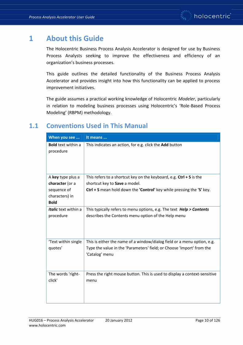
1.1 Conventions Used in This Manual
When you see ... It means ...
Bold text within a
procedure
This indicates an action, for e.g. click the Add button
A key type plus a
character (or a
sequence of
characters) in
Bold
This refers to a shortcut key on the keyboard, e.g. Ctrl + S is the
shortcut key to Save a model.
Ctrl + S mean hold down the 'Control' key while pressing the 'S' key.
Italic text within a
procedure
This typically refers to menu options, e.g. The text Help > Contents
describes the Contents menu option of the Help menu
‘Text within single
quotes’
This is either the name of a window/dialog field or a menu option, e.g.
Type the value in the 'Parameters' field; or Choose 'Import' from the
'Catalog' menu
The words 'right-
click'
Press the right mouse button. This is used to display a context-sensitive
menu
Process Analysis Accelerator User Guide
HUG016 – Process Analysis Accelerator 20 January 2012 Page 11 of 126 www.holocentric.com
2 Process Analysis in Context
2.1 What is Business Process Analysis? Business Process Analysis is an analytical tool which can be used to develop a detailed
understanding of an organization and to leverage this understanding to identify and
realize business performance improvement (BPI) opportunities.
Business process analysis, in turn, leverages business process modeling as a platform
for describing the many activities that an organization undertakes in pursuit of its
strategic intent and, in the case of a role-based Holocentric process model, also
identifying the organizational roles that perform or contribute to these activities.
Where a process model is sufficiently robust and sophisticated in nature (i.e. a
Holocentric process model), the model can be populated with role metrics (e.g. annual
cost) and activity metrics (e.g. time, overhead cost and transaction volumes) and
subsequently analysed to identify the process constraints and inefficiencies, leading to
the identification of candidate process improvement opportunities.
Delving a little deeper still, the analysis technique employed by Holocentric’s Process
Analysis Accelerator is known as Path Analysis. Path Analysis is an interrogation of a
role-based process model that identifies and resolves every possible process path
between a nominated start point and a nominated end point within the process
model. As each unique path is resolved by the analysis engine, all role and activity
metrics associated with that path are accumulated to allow detailed analysis of each
path.
The Process Analysis Accelerator also allows the simulation of candidate process
changes well in advance of actually implementing those changes. Thus, process
improvement strategies and underlying assumptions can be rigorously tested, in a
simulation ‘play-pen’, without putting the continuity and integrity of the real process
at risk.

Process Analysis Accelerator User Guide
HUG016 – Process Analysis Accelerator 20 January 2012 Page 12 of 126 www.holocentric.com
2.2 Why do Process Analysis? Many organizations operate within highly competitive and tightly resource constrained
environments. In such environments, it is not uncommon for ever greater returns to
be demanded of ever diminishing organizational resources. Process Analysis provides
an organization with the means to identify those processes that are wasteful or
inefficient to ensure that the organization’s finite resources are being utilised in the
most productive manner possible.
It is critically important that an organization is able to make a clear and unambiguous
appraisal of which processes are inefficient or value diluting. Using the results of such
analyses, informed process improvement strategies can be developed and
implemented with a higher degree of confidence that the changes employed will
actually yield the expected process improvement outcomes.
2.3 Which Processes Need Improvement? One straightforward measure of how effectively a process is performing is to calculate
its cycle efficiency1.
A process’ cycle efficiency can be expressed as a percentage and is calculated by
dividing the sum of the time taken to complete the value-adding steps within the
process by the total time taken to complete the entire process. For example, a process
may take a total of 2 hours to complete, whereas the sum of the time taken for the
value-adding process steps may total only 20 minutes. A process with these attributes
would be said to have a cycle efficiency of 16% (i.e. 20 minutes/120 minutes). Hence,
taking measures to eliminate the non-value adding activities and reduce the lag time
between the steps in the process would both be reasonable strategies to employ to
improve the cycle efficiency of the process.
All other things being equal, processes with low cycle efficiency are generally worthy of
attention from a process improvement perspective. However, making an assumption
that all processes are equal can be somewhat problematic. For example, a HR process
with a very low cycle efficiency that occurs only once a week may have much less
severe efficiency impact upon a business than a process with a higher cycle efficiency
that occurs many times a day in an area of high sensitivity e.g. Finance. Thus, the
criticality and significance of the process to the business should also be key
considerations when prioritising which processes deserve the most process
improvement attention.
ROCE – Achieving more with less...
1 Lean Six Sigma - Michael L. George
Process Analysis Accelerator User Guide
HUG016 – Process Analysis Accelerator 20 January 2012 Page 13 of 126 www.holocentric.com
Another useful measure for assessing the relative performance of a business process is
to determine the level of value ‘returned’ by a process in respect to the level of
organizational resources ‘consumed’ by that same process. This type of performance
assessment is known as ‘Return on Capital Employed’ or ROCE.
According to Wikipedia, “Return on Capital Employed (ROCE) is used in finance as a
measure of the returns that a company is realizing from its capital employed. It is
commonly used as a measure for comparing the performance between businesses and
for assessing whether a business generates enough returns to pay for its cost of
capital2”.
Whilst often used in financial contexts to assess the value that an entire organization
returns for the level of capital employed by that organization, the ROCE measure is
equally applicable when scaled to a process level of assessment.
ROCE can be used as an indicator of process performance whereby the inputs or
resources consumed by the process e.g. financial, people, technology, products,
services (i.e. the capital) can be compared to the value realized by the process (i.e. the
return). Hence, processes with a positive ROCE are therefore delivering more value to
a business than the sum of the resources that are consumed by the process. A process
with a negative ROCE would therefore be considered a value diluting process.
From a practical stand point, quantifying the level of resources consumed by a
business process is a much more straightforward analytical task as opposed
quantifying the true value realized by the process. For example, the ‘value’ of some
process outcomes may be quite subjective e.g. improved quality or reduced lead times
may be important to some customers, but not so to others.
Thus, placing a strong focus upon reducing the capital employed by a process (e.g.
taking less time and resource to perform the same process) is generally a more
practical and potent method of achieving tangible and sustainable process
improvement outcomes. The underlying assumption here of course is that the process
is actually realizing the value currently expected of it, we just want to see if we can
sustain this level of value output but use less internal capital to do so.
2 Wikipedia. The free encyclopaedia
Process Analysis Accelerator User Guide
HUG016 – Process Analysis Accelerator 20 January 2012 Page 14 of 126 www.holocentric.com
2.4 What is Path Analysis? Path Analysis involves the study of all of the possible, and often likely, ways of
navigating through a business process model between two specified points of interest.
The discrete paths identified through path analysis can be used as the basis of Time
Driven Activity Based Costing or, alternatively, to support Capacity Constraint Analysis
whereby capacity ‘bottlenecks’ within the process can be readily identified and
addressed.
The measurement of process effectiveness can vary between organizations however
there are several 'standard' metrics that can be used as a consistent starting point, viz:
Process Cost
Resource Utilisation
Relative Risk
Volume
Process Lead, Lag and Duration time

Process Analysis Accelerator User Guide
HUG016 – Process Analysis Accelerator 20 January 2012 Page 15 of 126 www.holocentric.com
3 Path Analysis in Holocentric Modeler Holocentric Modeler provides a Discrete Event process analysis capability that allows
current processes to be analyzed, improvements simulated and new processes to be
identified.
Through the use of scenario based process traversal definitions, performance metrics
including activity duration, lag times and volume are incrementally considered to
arrive at complete history graphs of an executed process scenario.
Problem areas can be easily identified - for example, activities that are too expensive,
resource-intensive, high risk, or low reliability. Costs of processes, performance
throughput, skills and staffing requirements can all be determined. Metrics can be
modified, such as the allocation of additional resources, the diverting of work down
different paths, and changes in volumes of work. Improvements can then be tested
and fine-tuned.
The tool can generate analysis results out to an Excel model, which allows for
comprehensive analysis of the definition and execution history to highlight resource
utilization, key constraint areas, estimated throughput and costing results. Weighted
statistical outcomes for activity volumes and work routes can also be incorporated
within the simulation model.
The simulation capabilities delivered within the product are positioned for pragmatic,
practical use by process managers and participants. Further advanced analysis for
dedicated simulation professionals can be analyzed using the raw generated XML file
and often by importing this file into more specialized simulation engines.
The metrics associated with processes and roles are exported from the models. These
metrics can then be modified in MS Excel® and the processing paths optimized. When
the information is pulled back into Holocentric Modeler, the impact across the
organization can be determined and implementation can be planned, with a detailed
understanding of how the changes will affect roles and supporting systems.
Holocentric Modeler supports two primary process analysis approaches the first being
Time Driven Activity Based Costing and the second being Capacity Constraint Analysis.
Process Analysis Accelerator User Guide
HUG016 – Process Analysis Accelerator 20 January 2012 Page 16 of 126 www.holocentric.com
3.1 Time Driven Activity Based Costing Time Driven Activity Based Costing (TDABC) is a pragmatic and effective technique for
analyzing processes based on estimated end-to-end processing times across a range of
processing paths weighted according to their share of volume.
TDABC focuses on how much it costs per time unit to supply resources to the business
activities and how much time it takes to carry out one unit of each kind of activity. It
exploits data generally available to subject matter experts to address the problems
such as inefficient processes, unprofitable product and service lines and optimizing
activity.
In the time driven process analysis view, you can use the Excel model to determine the
contribution to the processing cost and time that is made by each process path.
Within the time driven costing execution model, there is assumed to be an unlimited
capacity of labour and no pre-determined volume of activities. Instead, the model
simulates the execution of an annual number of complete process cycles with work
distributed over the various possible paths according to routing weightings that are
defined in the process model.
Holocentric's implementation of TDABC originated from practical experience in the
field and was subsequently confirmed by the writing of Robert Kaplan (of Balanced
Scorecard fame) and Steven Anderson (an international expert on Activity Based
Costing).
3.2 Capacity Constraint Analysis In the constraint based process analysis view, the Excel model can be used to
determine an organization’s ability to meet average daily work requirements based on
a fixed capacity of labour.
Within the constraint model, the maximum number of process paths that can be
executed is assumed to be limited by the type of labour that has the least capacity. In
the model, it is possible to adjust the percentage of work that will be performed across
each path in order to simulate changes to the available capacity and required volume
of activities.
3.3 Concepts Defined By analyzing an organization’s activities and the roles that are played by the people
and automated systems participating in those activities, it is possible to establish the
interdependencies, prerequisites and conditional branches that may occur during a
sequential performance of one activity leading to another, thus creating a Process
Flow. Using this approach, a simple yet comprehensive model can be constructed
Process Analysis Accelerator User Guide
HUG016 – Process Analysis Accelerator 20 January 2012 Page 17 of 126 www.holocentric.com
which describes all of the business processes and supporting systems that an
organization employs.
In Modeler, a process model typically consists of diagrams, their intent being to
describe a real-life process. These models are drawn as a series of Process Diagrams
that involve Actors, which more often than not represent the roles that people play in
a process. In the Process Analysis Accelerator individual Actors are typically
represented by their own pool lane.
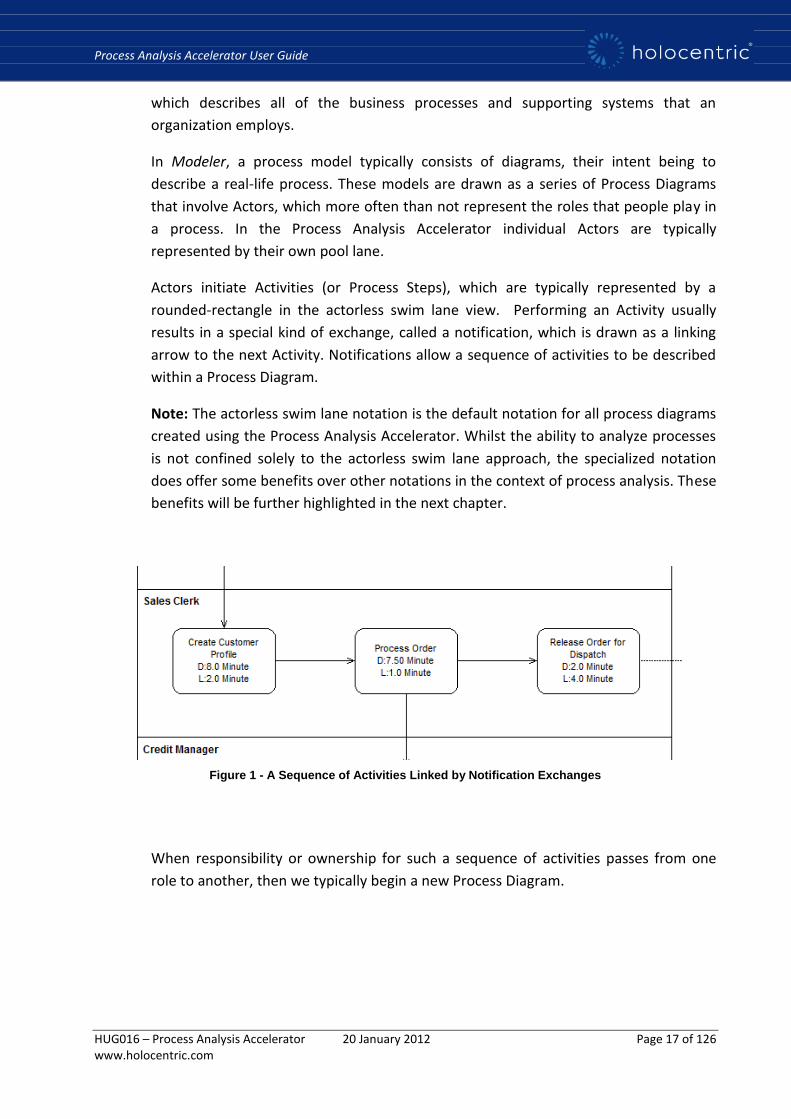
Actors initiate Activities (or Process Steps), which are typically represented by a
rounded-rectangle in the actorless swim lane view. Performing an Activity usually
results in a special kind of exchange, called a notification, which is drawn as a linking
arrow to the next Activity. Notifications allow a sequence of activities to be described
within a Process Diagram.
Note: The actorless swim lane notation is the default notation for all process diagrams
created using the Process Analysis Accelerator. Whilst the ability to analyze processes
is not confined solely to the actorless swim lane approach, the specialized notation
does offer some benefits over other notations in the context of process analysis. These
benefits will be further highlighted in the next chapter.
Figure 1 - A Sequence of Activities Linked by Notification Exchanges
When responsibility or ownership for such a sequence of activities passes from one
role to another, then we typically begin a new Process Diagram.
Process Analysis Accelerator User Guide
HUG016 – Process Analysis Accelerator 20 January 2012 Page 18 of 126 www.holocentric.com
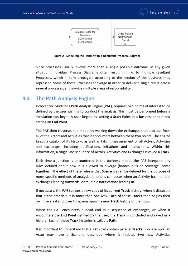
Figure 2 - Modeling the Hand-off to a Resultant Process Diagram
Since processes usually involve more than a single possible outcome, in any given
situation, individual Process Diagrams often result in links to multiple resultant
Processes, which in turn propagate according to the section of the business they
represent. Some of these Processes converge in order to deliver a single result across
several processes, and involve multiple areas of responsibility.
3.4 The Path Analysis Engine Holocentric Modeler’s Path Analysis Engine (PAE), requires two points of interest to be
defined by the user wishing to conduct the analysis. This must be performed before a
simulation can begin. A user begins by setting a Start Point in a business model and
setting an End Point.
The PAE then traverses the model by walking down the exchanges that lead out from
all of the Actors and Activities that it encounters between these two points. The engine
keeps a catalog of its history, as well as taking measurement of all Actors, Activities
and exchanges, including notifications, initiations and interactions. Within this
information, a single line-sequence of Actors, Activities and Exchanges is called a Track.
Each time a junction is encountered in the business model, the PAE interprets any
rules defined about how it is allowed to diverge (branch out) or converge (come
together). The effect of these rules is that Scenarios can be defined for the purpose of
more specific methods of analysis. Junctions can occur when an Activity has multiple
exchanges leading outwards, or multiple notifications leading in.
If necessary, the PAE spawns a new copy of its current Track history, when it discovers
that it can branch out in more than one way. Each of these Tracks then begins their
own traversal and, over time, may spawn a new Track history of their own.
When the PAE encounters a dead end in a sequence of exchanges, or when it
encounters the End Point defined by the user, the Track is concluded and saved as a
history. Each of these Track histories is called a Path.
It is important to understand that a Path can contain parallel Tracks. For example, an
Actor may have a Scenario described where it initiates two new Activities
Process Analysis Accelerator User Guide
HUG016 – Process Analysis Accelerator 20 January 2012 Page 19 of 126 www.holocentric.com
simultaneously. In this case, we refer to the Path as containing multiple Tracks or
Parallel Tracks.
Once all of the possible traversals are exhausted, the PAE is left with a collection of
Paths, some of which reach the defined End Point and some which do not. Depending
on the users requirements some, or even all, of these paths are then exported as XML
into a file.
An XML output file can be quite large and indeed is not usually conducive to being read
and understood on its own. Fortunately, Holocentric Modeler is shipped with a
specialized Microsoft Excel spreadsheet that can interpret the XML output file and
support some basic analysis.
3.5 Simulation Prerequisites In order to run a Simulation and create an output file describing the contents of Paths,
the Holocentric Modeler must be installed and have the correct set up options as
outlined below.
The spreadsheet shipped with Modeler is capable of interpreting the result of a
simulation when run using the default options available. Running a standard
simulation from the Modeler involves opening the spreadsheet, which in turn
processes the generated XML data. In order to perform analysis and use the
spreadsheet you must ensure the following:
Holocentric Modeler version 6 or later is installed
Your licence key allows access to the functionality of the Process Analysis
Accelerator
Excel 2000 or later is installed on the machine that is running Modeler.
Macros are enabled in Excel’s Security settings. If during the simulation you are
prompted whether or not to enable or disable macros, you will need to make sure that
macros are enabled. If not, the Path Analysis spreadsheet will not be able to process
the results of your simulation.
XML 2 is supported by the machine that is running Modeler. This would be true for any
machine that has Internet Explorer 4 or greater installed.
Process Analysis Accelerator User Guide
HUG016 – Process Analysis Accelerator 20 January 2012 Page 20 of 126 www.holocentric.com
4 Using the Process Analysis Accelerator
4.1 Modeling with Process Analysis in Mind In this section of the Process Analysis User Guide we will outline the subtle variations
in approach and additional actions required to create a process model in Holocentric
Modeler that will support detailed process analysis using the Process Analysis
Accelerator.
Firstly, we will introduce you to the specific nuances of modeling business processes
using the actorless swim lane notation, which is the default process notation of the
Process Analysis Accelerator. Secondly, we will outline the steps required to assign
metrics to the key process elements either using Modeler or by way of an
export/import approach, in conjunction with MS Excel. At the end of this section, we
will then describe how to apply volume constraints to key aspects of your processes
and to meaningfully account for both direct and indirect involvement of various roles
in fulfilling the business process.
4.2 Developing and Defining the Process In this section, we introduce the actorless swim lane process notation. The actorless
swim lane notation is the default notation for all process diagrams created using the
Process Analysis Accelerator. Whilst the ability to analyze processes is not confined
solely to the actorless swim lane approach, the specialized notation does offer some
benefits over other notations in the context of process analysis. The use of the Process
Analysis Accelerator with other process notations is discussed in Appendix 1.
4.3 Introducing the Actorless Swim Lane Notation
4.3.1 Background
Process modeling using the Process Analysis Accelerator is very similar to the general
use of Holocentric for business process modeling. However, there are a few unique
aspects of the Accelerator’s default process modeling notation that may need to be
taken into consideration.
The Accelerator introduces a new default library under the Business & Enterprise
category. When using this default library to create a new project, the defaulting
diagram notation for process diagrams will result in an actorless swim lanes style of
diagram i.e. each actor in the process is represented by an individual pool lane. Even
though structurally present, the individual actor representations (e.g. between process
steps) are generally hidden from view. This style of diagram results in a succinct view

Process Analysis Accelerator User Guide
HUG016 – Process Analysis Accelerator 20 January 2012 Page 21 of 126 www.holocentric.com
of the process activities and also enables the display of key metrics against these
activities.
Figure 3 - Actorless Swim Lane Process Diagram Notation
The default process diagram notation of the Accelerator can be easily overridden at a
diagram level by changing the notation, or library wide, by using a diagram template.
The process analysis approach is equally effective on the traditional role-based ‘graph’
notation and can also be readily applied to existing models.
The following section will outline the subtle variations of the actorless swim lane
notation when used to model a simple business process. Whilst slight variations in
approach may be required across the different diagram notations available in
Holocentric Modeler, these variations will be outlined in greater detail in Appendix 1,
as will the approach required to enable process analysis upon an existing model.
4.3.2 Prerequisites
Before modeling a business process using the Process Analysis accelerator, you should
ensure that the following requirements have been satisfied:

Process Analysis Accelerator User Guide
HUG016 – Process Analysis Accelerator 20 January 2012 Page 22 of 126 www.holocentric.com
You are already familiar with the general use of Holocentric in the context of
modeling role-based business processes
You have a licence key installed that enables the functionality provided by the
process analysis accelerator.
At a minimum, the ‘Business Process Analysis Analyst’ and ‘System Architect’ user
perspectives (Tools > Options > User Perspectives) should be active. Alternatively,
choosing ‘All Perspectives’ will activate all possible views, but as a consequence,
this will also increase the complexity of menus and range of user options.

Process Analysis Accelerator User Guide
HUG016 – Process Analysis Accelerator 20 January 2012 Page 23 of 126 www.holocentric.com
4.3.3 Directions
4.3.3.1 Creating a New Process Analysis library
Open Holocentric Modeler and create a new library using the ‘Process Analysis Library’
default library as follows.
Figure 4 - Process Analysis Default Library
Make sure that you name and save your library in an appropriate location and set your
preferred auto-save settings under Library > Properties > Save.
4.3.3.2 Creating a New Process Diagram
Click on the ‘Model Scope’ link on the home page to open the Model Scope diagram.
Using the ‘Process Diagram Selection’ tool , create and place a new process diagram
named ‘Customer Orders’ onto the ‘Model Scope’ diagram. Open the new diagram by
double-clicking upon its icon.
One of the first things you may notice is the changed appearance of the toolbox and
the presence of a default pool lane on the process diagram canvas. The toolbox,
whilst similar to the standard process diagram toolbox, also presents a range of tools
that are specifically related to modeling processes using the actorless swim lane
notation. The purpose of the specialized tools will be covered shortly.
Process Analysis Accelerator User Guide
HUG016 – Process Analysis Accelerator 20 January 2012 Page 24 of 126 www.holocentric.com
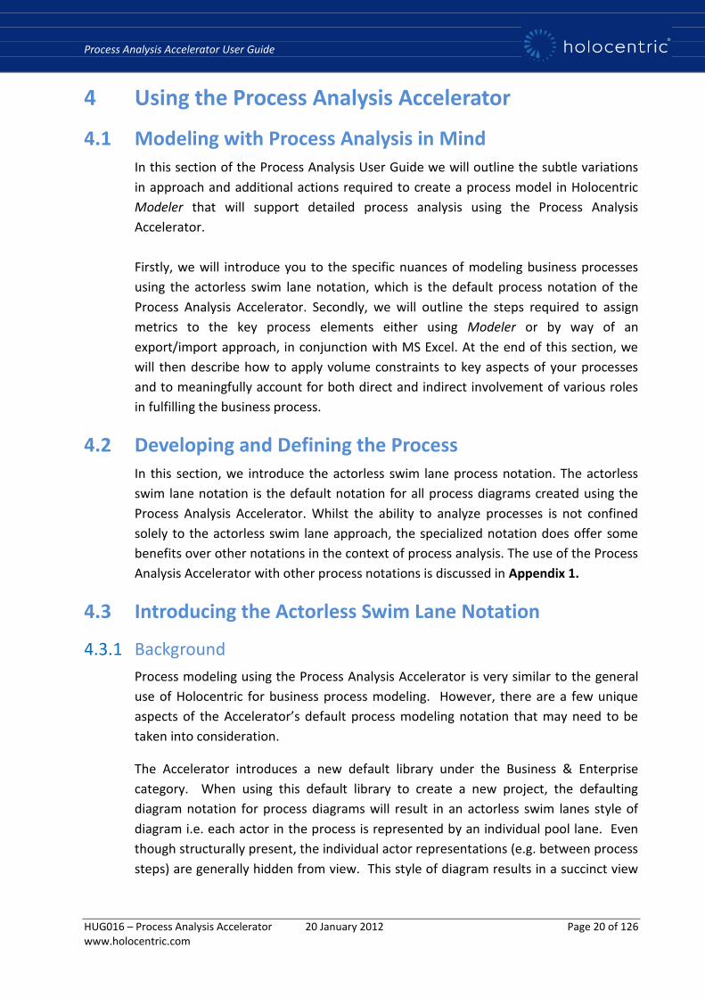
Figure 5 - Actorless Swim Lane Toolbox
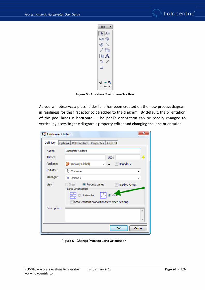
As you will observe, a placeholder lane has been created on the new process diagram
in readiness for the first actor to be added to the diagram. By default, the orientation
of the pool lanes is horizontal. The pool’s orientation can be readily changed to
vertical by accessing the diagram’s property editor and changing the lane orientation.
Figure 6 - Change Process Lane Orientation
Process Analysis Accelerator User Guide
HUG016 – Process Analysis Accelerator 20 January 2012 Page 25 of 126 www.holocentric.com
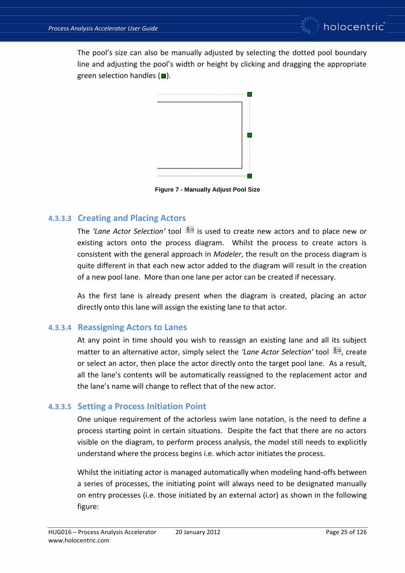
The pool’s size can also be manually adjusted by selecting the dotted pool boundary
line and adjusting the pool’s width or height by clicking and dragging the appropriate
green selection handles ( ).
Figure 7 - Manually Adjust Pool Size
4.3.3.3 Creating and Placing Actors
The ‘Lane Actor Selection’ tool is used to create new actors and to place new or
existing actors onto the process diagram. Whilst the process to create actors is
consistent with the general approach in Modeler, the result on the process diagram is
quite different in that each new actor added to the diagram will result in the creation
of a new pool lane. More than one lane per actor can be created if necessary.
As the first lane is already present when the diagram is created, placing an actor
directly onto this lane will assign the existing lane to that actor.
4.3.3.4 Reassigning Actors to Lanes
At any point in time should you wish to reassign an existing lane and all its subject
matter to an alternative actor, simply select the ‘Lane Actor Selection’ tool , create
or select an actor, then place the actor directly onto the target pool lane. As a result,
all the lane’s contents will be automatically reassigned to the replacement actor and
the lane’s name will change to reflect that of the new actor.
4.3.3.5 Setting a Process Initiation Point
One unique requirement of the actorless swim lane notation, is the need to define a
process starting point in certain situations. Despite the fact that there are no actors
visible on the diagram, to perform process analysis, the model still needs to explicitly
understand where the process begins i.e. which actor initiates the process.
Whilst the initiating actor is managed automatically when modeling hand-offs between
a series of processes, the initiating point will always need to be designated manually
on entry processes (i.e. those initiated by an external actor) as shown in the following
figure:

Process Analysis Accelerator User Guide
HUG016 – Process Analysis Accelerator 20 January 2012 Page 26 of 126 www.holocentric.com
Figure 8 - Process Initiation Point
To designate the process initiation point, simply click on the ‘Initiator Actor Selection’
tool and click to place the node into the lane that represents the initiating actor, in
this example the Customer initiates the process by placing an order. Placing the
initiation point in an actor’s lane will also assign that actor to the ‘Initiator’ field under
the diagram’s properties.
4.3.3.6 Creating Process Steps
With the required actors created and placed onto the diagram as lanes, we can now
turn our attention to modeling the sequences of activities that constitute the business
process. Under the actorless swim lane notation, activities (also known as Use Cases)
are referred to as ‘Process Steps’. Process steps are added to the diagram using the
‘Process Step Selection’ tool . When adding process steps to a process diagram, the
steps should be placed directly into the lane of the actor that actually performs the
work.
Depending upon the specific attributes chosen for the process step, the nature of the
node displayed will vary. For example, if the process step is designated as IT
Dependent (i.e. Parent = Base Activity) the shape will display a solid border.
Figure 9 - IT Dependent Process Step
Alternatively, if the process step is designated as being Manual (i.e. Parent = Base Task)
a dashed border will be displayed.

Process Analysis Accelerator User Guide
HUG016 – Process Analysis Accelerator 20 January 2012 Page 27 of 126 www.holocentric.com
Figure 10 - Manual Process Step
If no parent value as been assigned, a node with a dotted border and a subtle fill color
will be displayed.
Figure 11 - No Parent Defined
Finally, if the process step is flagged as being a decision point, a more traditional
diamond-shaped node will be displayed.
Figure 12 - Flagged as a Decision
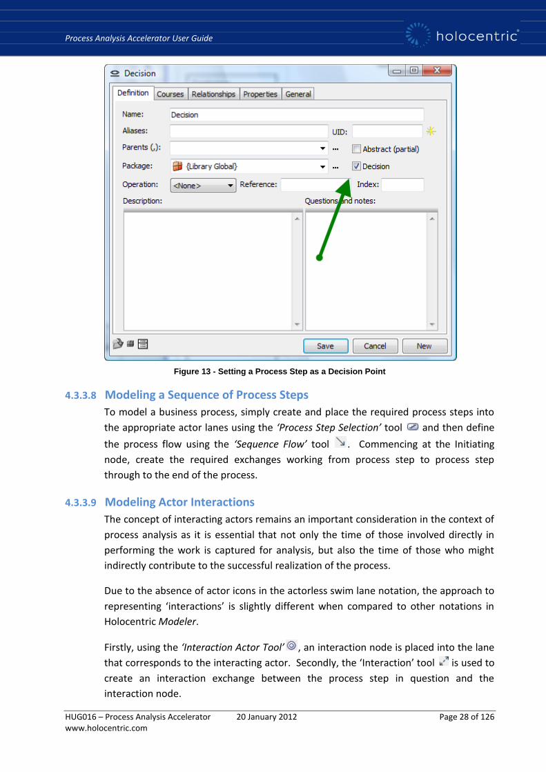
4.3.3.7 Designating a Process Step as Decision Point
To designate a process step as a decision point, simply check the ‘Decision’ checkbox
under the process step’s property editor as shown:
Process Analysis Accelerator User Guide
HUG016 – Process Analysis Accelerator 20 January 2012 Page 28 of 126 www.holocentric.com
Figure 13 - Setting a Process Step as a Decision Point
4.3.3.8 Modeling a Sequence of Process Steps
To model a business process, simply create and place the required process steps into
the appropriate actor lanes using the ‘Process Step Selection’ tool and then define
the process flow using the ‘Sequence Flow’ tool . Commencing at the Initiating
node, create the required exchanges working from process step to process step
through to the end of the process.
4.3.3.9 Modeling Actor Interactions
The concept of interacting actors remains an important consideration in the context of
process analysis as it is essential that not only the time of those involved directly in
performing the work is captured for analysis, but also the time of those who might
indirectly contribute to the successful realization of the process.
Due to the absence of actor icons in the actorless swim lane notation, the approach to
representing ‘interactions’ is slightly different when compared to other notations in
Holocentric Modeler.
Firstly, using the ‘Interaction Actor Tool’ , an interaction node is placed into the lane
that corresponds to the interacting actor. Secondly, the ‘Interaction’ tool is used to
create an interaction exchange between the process step in question and the
interaction node.
Process Analysis Accelerator User Guide
HUG016 – Process Analysis Accelerator 20 January 2012 Page 29 of 126 www.holocentric.com
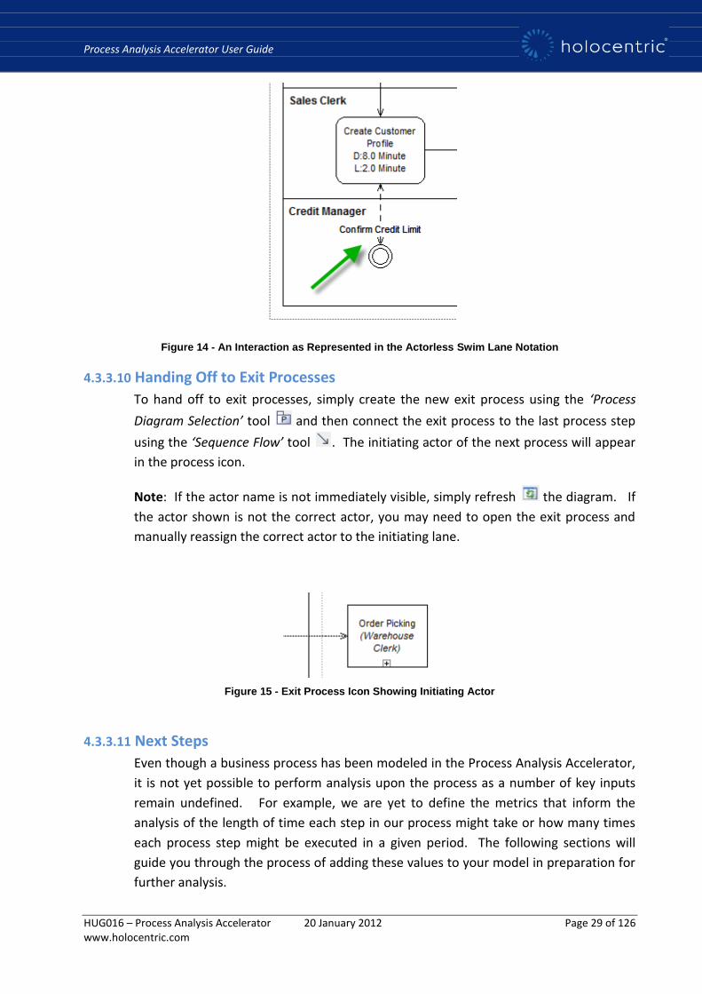
Figure 14 - An Interaction as Represented in the Actorless Swim Lane Notation
4.3.3.10 Handing Off to Exit Processes
To hand off to exit processes, simply create the new exit process using the ‘Process
Diagram Selection’ tool and then connect the exit process to the last process step
using the ‘Sequence Flow’ tool . The initiating actor of the next process will appear
in the process icon.
Note: If the actor name is not immediately visible, simply refresh the diagram. If
the actor shown is not the correct actor, you may need to open the exit process and
manually reassign the correct actor to the initiating lane.
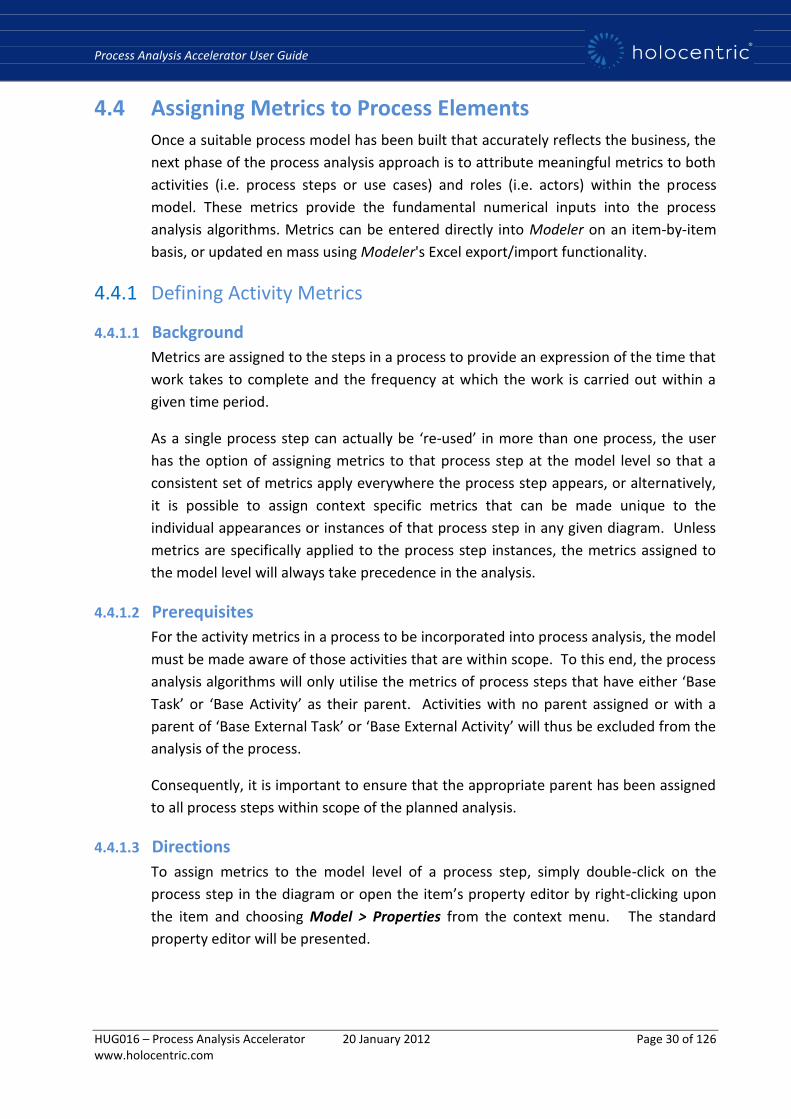
Figure 15 - Exit Process Icon Showing Initiating Actor
4.3.3.11 Next Steps
Even though a business process has been modeled in the Process Analysis Accelerator,
it is not yet possible to perform analysis upon the process as a number of key inputs
remain undefined. For example, we are yet to define the metrics that inform the
analysis of the length of time each step in our process might take or how many times
each process step might be executed in a given period. The following sections will
guide you through the process of adding these values to your model in preparation for
further analysis.
Process Analysis Accelerator User Guide
HUG016 – Process Analysis Accelerator 20 January 2012 Page 30 of 126 www.holocentric.com
4.4 Assigning Metrics to Process Elements Once a suitable process model has been built that accurately reflects the business, the
next phase of the process analysis approach is to attribute meaningful metrics to both
activities (i.e. process steps or use cases) and roles (i.e. actors) within the process
model. These metrics provide the fundamental numerical inputs into the process
analysis algorithms. Metrics can be entered directly into Modeler on an item-by-item
basis, or updated en mass using Modeler's Excel export/import functionality.
4.4.1 Defining Activity Metrics
4.4.1.1 Background
Metrics are assigned to the steps in a process to provide an expression of the time that
work takes to complete and the frequency at which the work is carried out within a
given time period.
As a single process step can actually be ‘re-used’ in more than one process, the user
has the option of assigning metrics to that process step at the model level so that a
consistent set of metrics apply everywhere the process step appears, or alternatively,
it is possible to assign context specific metrics that can be made unique to the
individual appearances or instances of that process step in any given diagram. Unless
metrics are specifically applied to the process step instances, the metrics assigned to
the model level will always take precedence in the analysis.
4.4.1.2 Prerequisites
For the activity metrics in a process to be incorporated into process analysis, the model
must be made aware of those activities that are within scope. To this end, the process
analysis algorithms will only utilise the metrics of process steps that have either ‘Base
Task’ or ‘Base Activity’ as their parent. Activities with no parent assigned or with a
parent of ‘Base External Task’ or ‘Base External Activity’ will thus be excluded from the
analysis of the process.
Consequently, it is important to ensure that the appropriate parent has been assigned
to all process steps within scope of the planned analysis.
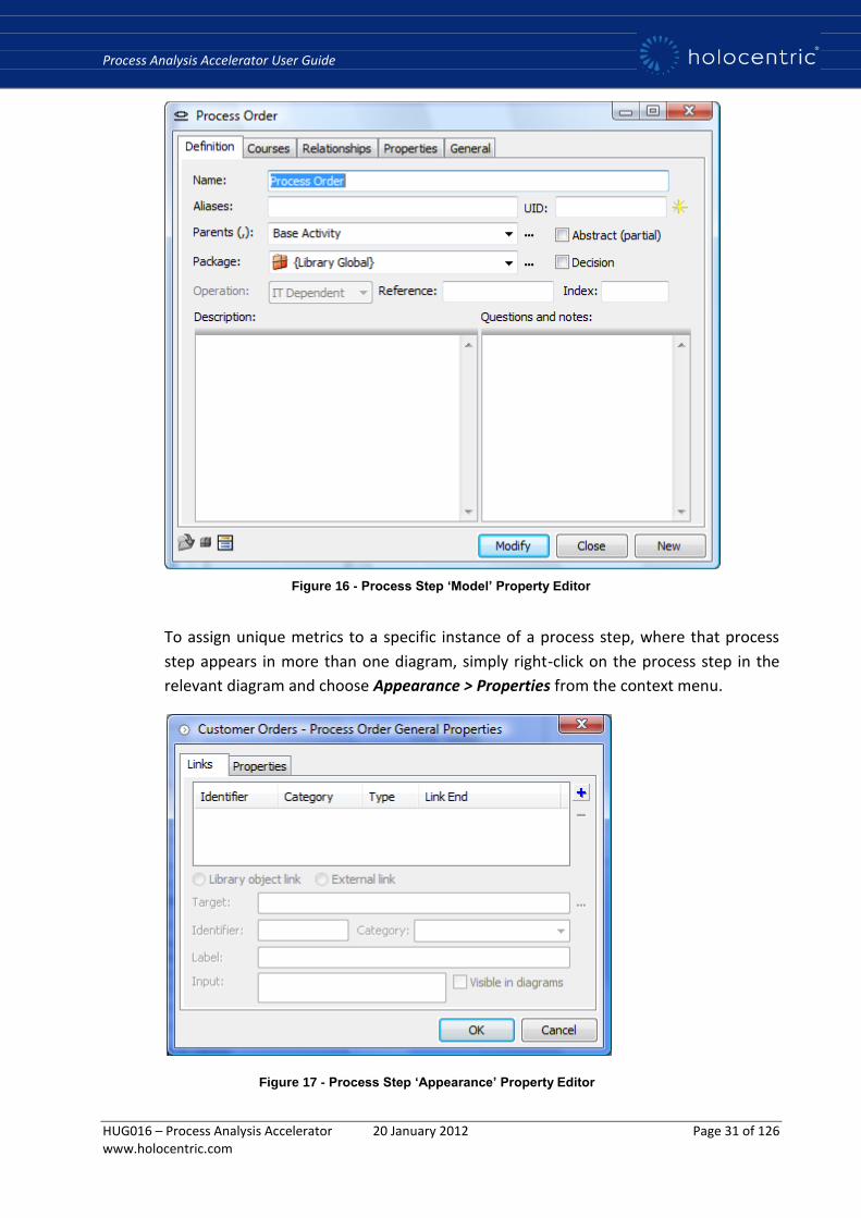
4.4.1.3 Directions
To assign metrics to the model level of a process step, simply double-click on the
process step in the diagram or open the item’s property editor by right-clicking upon
the item and choosing Model > Properties from the context menu. The standard
property editor will be presented.
Process Analysis Accelerator User Guide
HUG016 – Process Analysis Accelerator 20 January 2012 Page 31 of 126 www.holocentric.com
Figure 16 - Process Step ‘Model’ Property Editor
To assign unique metrics to a specific instance of a process step, where that process
step appears in more than one diagram, simply right-click on the process step in the
relevant diagram and choose Appearance > Properties from the context menu.
Figure 17 - Process Step ‘Appearance’ Property Editor

Process Analysis Accelerator User Guide
HUG016 – Process Analysis Accelerator 20 January 2012 Page 32 of 126 www.holocentric.com
Whilst these two dialogs appear quite different in nature, the ‘Properties’ tab is
identical for both. To access the form that will allow data capture of the activity
metrics, select the ‘Properties’ tab of either dialog and choose the ‘Activity Metrics’
page.
Figure 18 - Activity Metrics Data Entry Form
The ‘Activity Metrics’ page provides a series of property fields to allow data capture of
a process step’s metrics. Whilst some of the property fields listed are qualitative in
nature (i.e. Core Value Activity, Activity Analysis Type, Activity Quality,
Comments/Assumptions), the remaining fields provide direct input into the process
analysis calculations.
The key metric values required for process analysis are outlined below:
Avg. Activity Duration
An expression of the average time taken to successfully complete the activity. Ideally,
this value should be based upon historical data or a time study of the process in action.
Avg. Activity Lag Time
The average lag time that occurs between the completion of the current process step
and the commencement of the next immediate process step. Ideally, this value should
be based upon historical data or a time study of the process in action.
Process Analysis Accelerator User Guide
HUG016 – Process Analysis Accelerator 20 January 2012 Page 33 of 126 www.holocentric.com
Activity Unit of Time
The standard unit of time to be applied to the ‘Activity Duration’ and ‘Activity Lag
Time’ values e.g. minute, hour, day. Choose a time unit that is most appropriate for
the nature of the process. Note: It is advisable to use a consistent unit of time (e.g.
minutes) for all activities in a process model.
Avg. Cost Per Activity
The average cost of performing the process step e.g. consumables, overhead costs.
This value should only take into account the costs incurred over and above the time of
the people or systems involved. Resource costs for people and system utilisation are
directly catered for as part of the analysis.
Avg. Daily Volume
The average number of cycles per day for the process step i.e. how many times a day
on average the task would be performed. Ideally, this value should be based upon
historical transaction data.
Showing metrics on a process diagram
If desired, it is possible to show a brief summary of the most pertinent metrics within
the layout of the process diagram. To reveal the metric values against each process
step, open the required process diagram; use CTRL + A to deselect all items, then right-
click anywhere on the diagram canvas. From the resulting context menu, select
Properties, then select the ‘Properties’ tab.
Process Analysis Accelerator User Guide
HUG016 – Process Analysis Accelerator 20 January 2012 Page 34 of 126 www.holocentric.com
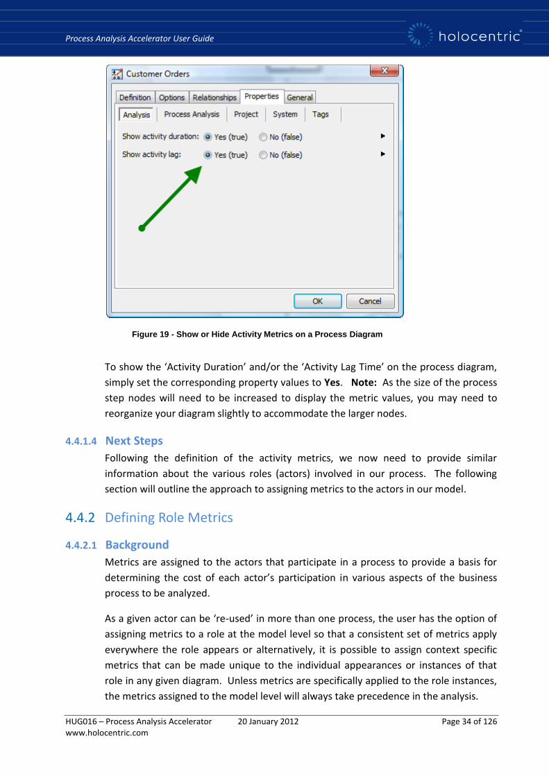
Figure 19 - Show or Hide Activity Metrics on a Process Diagram
To show the ‘Activity Duration’ and/or the ‘Activity Lag Time’ on the process diagram,
simply set the corresponding property values to Yes. Note: As the size of the process
step nodes will need to be increased to display the metric values, you may need to
reorganize your diagram slightly to accommodate the larger nodes.
4.4.1.4 Next Steps
Following the definition of the activity metrics, we now need to provide similar
information about the various roles (actors) involved in our process. The following
section will outline the approach to assigning metrics to the actors in our model.
4.4.2 Defining Role Metrics
4.4.2.1 Background
Metrics are assigned to the actors that participate in a process to provide a basis for
determining the cost of each actor’s participation in various aspects of the business
process to be analyzed.
As a given actor can be ‘re-used’ in more than one process, the user has the option of
assigning metrics to a role at the model level so that a consistent set of metrics apply
everywhere the role appears or alternatively, it is possible to assign context specific
metrics that can be made unique to the individual appearances or instances of that
role in any given diagram. Unless metrics are specifically applied to the role instances,
the metrics assigned to the model level will always take precedence in the analysis.
Process Analysis Accelerator User Guide
HUG016 – Process Analysis Accelerator 20 January 2012 Page 35 of 126 www.holocentric.com
4.4.2.2 Prerequisites
For the role metrics in a process to be incorporated into process analysis, the model
must be made aware of those roles that are within scope. To this end, the process
analysis algorithms will only utilise the metrics of roles that have ‘Base Internal’ as
their parent. Roles with no parent assigned or with a parent of ‘Base External’ will be
considered out of scope and thus excluded from the analysis of the process.
Consequently, it is important to ensure that the appropriate parent has been assigned
to all roles that will participate or provide some form of contribution within the scope
of the planned analysis.
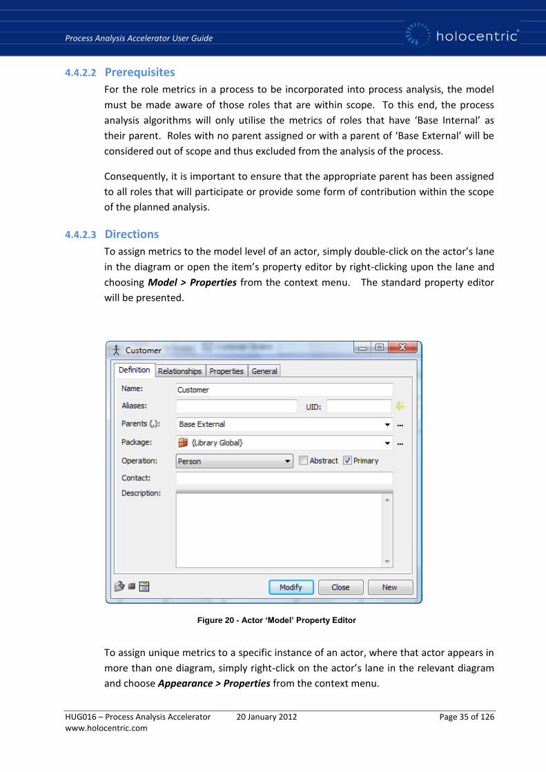
4.4.2.3 Directions
To assign metrics to the model level of an actor, simply double-click on the actor’s lane
in the diagram or open the item’s property editor by right-clicking upon the lane and
choosing Model > Properties from the context menu. The standard property editor
will be presented.
Figure 20 - Actor ‘Model’ Property Editor
To assign unique metrics to a specific instance of an actor, where that actor appears in
more than one diagram, simply right-click on the actor’s lane in the relevant diagram
and choose Appearance > Properties from the context menu.
Process Analysis Accelerator User Guide
HUG016 – Process Analysis Accelerator 20 January 2012 Page 36 of 126 www.holocentric.com
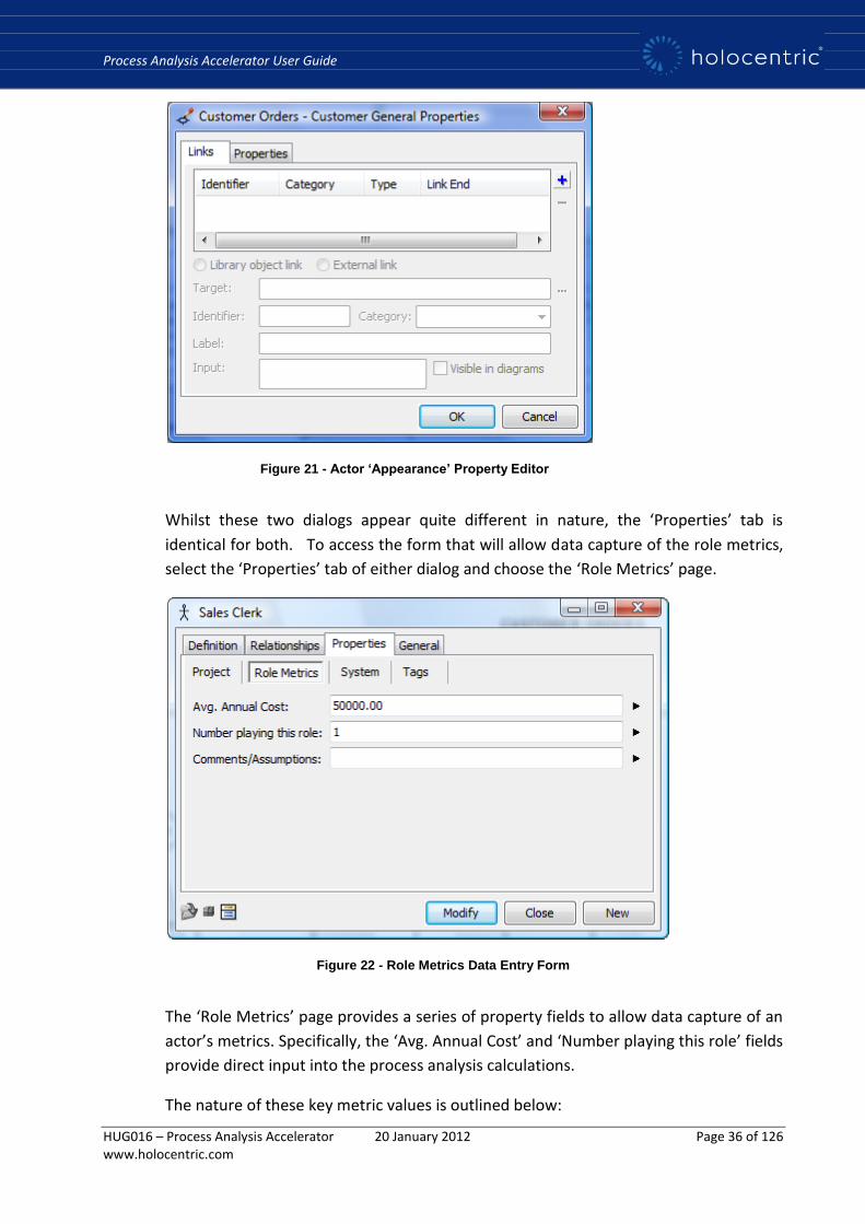
Figure 21 - Actor ‘Appearance’ Property Editor
Whilst these two dialogs appear quite different in nature, the ‘Properties’ tab is
identical for both. To access the form that will allow data capture of the role metrics,
select the ‘Properties’ tab of either dialog and choose the ‘Role Metrics’ page.
Figure 22 - Role Metrics Data Entry Form
The ‘Role Metrics’ page provides a series of property fields to allow data capture of an
actor’s metrics. Specifically, the ‘Avg. Annual Cost’ and ‘Number playing this role’ fields
provide direct input into the process analysis calculations.
The nature of these key metric values is outlined below:
Process Analysis Accelerator User Guide
HUG016 – Process Analysis Accelerator 20 January 2012 Page 37 of 126 www.holocentric.com
Avg. Annual Cost
An expression of the average annual cost to the organization of a given role. Ideally,
this value should be based upon real data (e.g. payroll data). Note: If there are a
range of individuals with varying salaries that perform the same role in a process, then
an appropriately weighted average cost for that group of employees should be
determined and applied to the relevant role.
Number playing this role
This metric allows the number of people performing a given role to be taken into
account during process analysis, particularly in respect to determining the capacity of a
given process.
4.4.2.4 Next Steps
The preceding sections have outlined the means to add both Activity Metrics and Role
Metrics to your model. The methods shown in these sections have focused entirely
upon a manual approach whereby the metrics for actors and process steps are
updated exclusively within Holocentric Modeler, one item at a time. Whilst this is can
be an acceptable approach if dealing with smaller models, the task of updating and
maintaining a large range of metrics can become challenging as the model size and
complexity grows.
The following sections offer an alternative approach to managing the metrics in your
model whereby Modeler’s MS Excel® export/import functionality is embraced to allow
more expedient management of a large number of metric values.
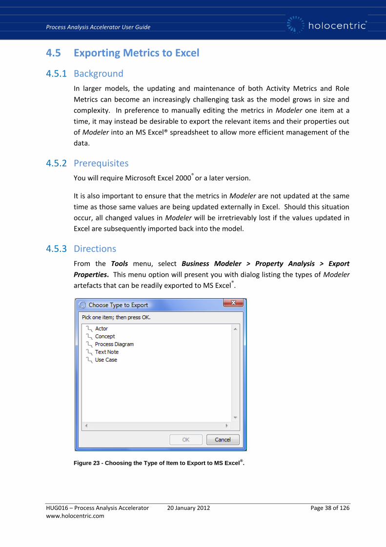
Process Analysis Accelerator User Guide
HUG016 – Process Analysis Accelerator 20 January 2012 Page 38 of 126 www.holocentric.com
4.5 Exporting Metrics to Excel
4.5.1 Background
In larger models, the updating and maintenance of both Activity Metrics and Role
Metrics can become an increasingly challenging task as the model grows in size and
complexity. In preference to manually editing the metrics in Modeler one item at a
time, it may instead be desirable to export the relevant items and their properties out
of Modeler into an MS Excel® spreadsheet to allow more efficient management of the
data.
4.5.2 Prerequisites
You will require Microsoft Excel 2000® or a later version.
It is also important to ensure that the metrics in Modeler are not updated at the same
time as those same values are being updated externally in Excel. Should this situation
occur, all changed values in Modeler will be irretrievably lost if the values updated in
Excel are subsequently imported back into the model.
4.5.3 Directions
From the Tools menu, select Business Modeler > Property Analysis > Export
Properties. This menu option will present you with dialog listing the types of Modeler
artefacts that can be readily exported to MS Excel®.
Figure 23 - Choosing the Type of Item to Export to MS Excel®.
Process Analysis Accelerator User Guide
HUG016 – Process Analysis Accelerator 20 January 2012 Page 39 of 126 www.holocentric.com
As we are primarily concerned with Actors or Process Steps (Use Cases), either of these
options can be chosen for export. Please note that only one item type at a time can be
exported, so this process will need to be carried out for both Actors and Process Steps.
Upon choosing an item type and clicking OK, you will be prompted to choose a location
where your export file will be saved to. Choose a suitable location e.g. Desktop. The
default format for the MS Excel® export is a comma separated variable file (.csv).
Having nominated a file location, you will next be prompted to view the exported
values. Choose Yes to launch Excel and open the export file in readiness for editing.
4.5.4 Next Steps
Now that an export of our metric values has been generated, the next section will
outline the steps required to update the metrics using MS Excel® in readiness for
import back into Modeler.
4.6 Editing Exported Metrics within Excel
4.6.1 Background
Following an export of model items and their properties from Modeler, these
properties can now be edited within MS Excel® in preparation for importing back into
Modeler as replacement values. As the MS Excel® property export is a generic export
capability you may find that much of the content returned in the spreadsheet is not
directly related to process analysis. Nonetheless, it is quite straightforward to organize
the spreadsheet into a more relevant and user friendly format.
4.6.2 Prerequisites
Some general experience in the use of MS Excel® is a useful prerequisite, but most
importantly, access to, or knowledge of, the required metrics for both process steps
and actors is essential.
4.6.3 Directions
Whilst the spreadsheet layout can remain unchanged and properties can be edited
directly into the appropriate cells, you may find it easier to spend a minute or two
making the most important elements of the spreadsheet more accessible. This is
particularly relevant if dealing with a large number of model artefacts and their
properties.
Hide columns
One of the easiest measures to take is to hide the columns that are not directly related
to process analysis and widen the remaining columns to a suitable width. The columns

Process Analysis Accelerator User Guide
HUG016 – Process Analysis Accelerator 20 January 2012 Page 40 of 126 www.holocentric.com
outlined below are the most relevant to the elements of process analysis. Thus, all
other columns can be safely hidden:
Key columns for process steps (Use Case) export
Name
avgActivityDuration
avgActivityDurationTimeUnit*
avgCostPerActivity
avgActivityLag
avgDailyVolume
Key columns for Actor export
Name
avgAnnualCost
numberOfPeople
*The avgActivityDurationTimeUnit field stores the time units as a decimal conversion
value. Please use the following values if updating this column within the spreadsheet:
Time Unit Conversion Value
Second 0.0003
Minute 0.0167
Hour 1.0000
Day 8.0000
Week 40.0000
Month 173.0000
Year 2080.0000
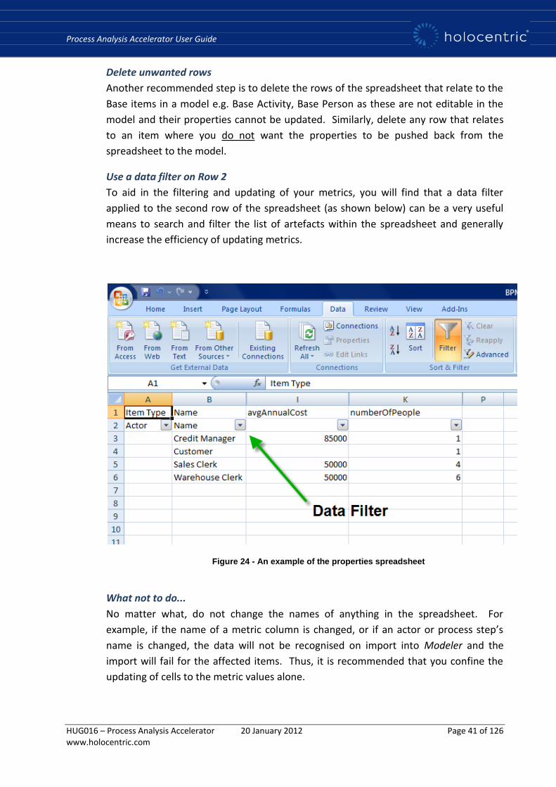
Process Analysis Accelerator User Guide
HUG016 – Process Analysis Accelerator 20 January 2012 Page 41 of 126 www.holocentric.com
Delete unwanted rows
Another recommended step is to delete the rows of the spreadsheet that relate to the
Base items in a model e.g. Base Activity, Base Person as these are not editable in the
model and their properties cannot be updated. Similarly, delete any row that relates
to an item where you do not want the properties to be pushed back from the
spreadsheet to the model.
Use a data filter on Row 2
To aid in the filtering and updating of your metrics, you will find that a data filter
applied to the second row of the spreadsheet (as shown below) can be a very useful
means to search and filter the list of artefacts within the spreadsheet and generally
increase the efficiency of updating metrics.
Figure 24 - An example of the properties spreadsheet
What not to do...
No matter what, do not change the names of anything in the spreadsheet. For
example, if the name of a metric column is changed, or if an actor or process step’s
name is changed, the data will not be recognised on import into Modeler and the
import will fail for the affected items. Thus, it is recommended that you confine the
updating of cells to the metric values alone.
Process Analysis Accelerator User Guide
HUG016 – Process Analysis Accelerator 20 January 2012 Page 42 of 126 www.holocentric.com
4.6.4 Results/Next Steps
Once metrics values have been successfully updated within the spreadsheet, you will
need to save your changes in readiness for import. Make sure that the spreadsheet is
saved in its original .csv format as this is the format that is required for import back
into Modeler.
Please note: Saving the spreadsheet to .csv format will result in the loss of any layout
changes (e.g. column widths, hidden columns, data filters) that you may have applied
to the spreadsheet during the editing process. If metrics are required to be edited
over one or more sessions in MS Excel®, then it is advisable to save the spreadsheet to
an .xls format in between these sessions and only save as .csv format once changes are
complete and ready for import.
In the following section, we will outline the steps required to import the updated
metrics spreadsheet back into Modeler.
4.7 Importing Updated Metrics from Excel
4.7.1 Background
Having exported and edited property values in MS Excel® it is now possible to import
the updated metric values back into your model using the property import
functionality.
4.7.2 Prerequisites
Prior to any import of data into your model, it is highly recommended that you take a
back up copy of your Modeler library so that recovery of previous property values is
easily accomplished, should the need arise.
You will need to have saved the Excel spreadsheet with the updated metrics in a
comma separated variable (.csv) file format.
4.7.3 Directions
To commence the import process, select Business Modeler > Property Analysis >
Import Properties from the Tools menu. You will then be prompted to locate the
source file.
Once you have located the source file and selected the Open button, you will be asked
to confirm that you wish the property values in the model to be updated with those in
the spreadsheet. Click OK to proceed.
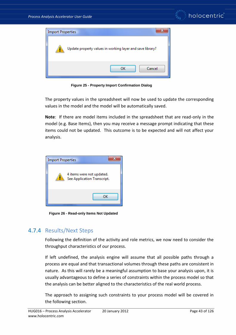
Process Analysis Accelerator User Guide
HUG016 – Process Analysis Accelerator 20 January 2012 Page 43 of 126 www.holocentric.com
Figure 25 - Property Import Confirmation Dialog
The property values in the spreadsheet will now be used to update the corresponding
values in the model and the model will be automatically saved.
Note: If there are model items included in the spreadsheet that are read-only in the
model (e.g. Base Items), then you may receive a message prompt indicating that these
items could not be updated. This outcome is to be expected and will not affect your
analysis.
Figure 26 - Read-only Items Not Updated
4.7.4 Results/Next Steps
Following the definition of the activity and role metrics, we now need to consider the
throughput characteristics of our process.
If left undefined, the analysis engine will assume that all possible paths through a
process are equal and that transactional volumes through these paths are consistent in
nature. As this will rarely be a meaningful assumption to base your analysis upon, it is
usually advantageous to define a series of constraints within the process model so that
the analysis can be better aligned to the characteristics of the real world process.
The approach to assigning such constraints to your process model will be covered in
the following section.
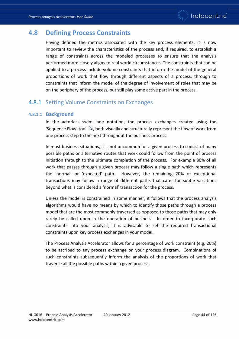
Process Analysis Accelerator User Guide
HUG016 – Process Analysis Accelerator 20 January 2012 Page 44 of 126 www.holocentric.com
4.8 Defining Process Constraints Having defined the metrics associated with the key process elements, it is now
important to review the characteristics of the process and, if required, to establish a
range of constraints across the modeled processes to ensure that the analysis
performed more closely aligns to real world circumstances. The constraints that can be
applied to a process include volume constraints that inform the model of the general
proportions of work that flow through different aspects of a process, through to
constraints that inform the model of the degree of involvement of roles that may be
on the periphery of the process, but still play some active part in the process.
4.8.1 Setting Volume Constraints on Exchanges
4.8.1.1 Background
In the actorless swim lane notation, the process exchanges created using the
‘Sequence Flow’ tool , both visually and structurally represent the flow of work from
one process step to the next throughout the business process.
In most business situations, it is not uncommon for a given process to consist of many
possible paths or alternative routes that work could follow from the point of process
initiation through to the ultimate completion of the process. For example 80% of all
work that passes through a given process may follow a single path which represents
the ‘normal’ or ‘expected’ path. However, the remaining 20% of exceptional
transactions may follow a range of different paths that cater for subtle variations
beyond what is considered a ‘normal’ transaction for the process.
Unless the model is constrained in some manner, it follows that the process analysis
algorithms would have no means by which to identify those paths through a process
model that are the most commonly traversed as opposed to those paths that may only
rarely be called upon in the operation of business. In order to incorporate such
constraints into your analysis, it is advisable to set the required transactional
constraints upon key process exchanges in your model.
The Process Analysis Accelerator allows for a percentage of work constraint (e.g. 20%)
to be ascribed to any process exchange on your process diagram. Combinations of
such constraints subsequently inform the analysis of the proportions of work that
traverse all the possible paths within a given process.
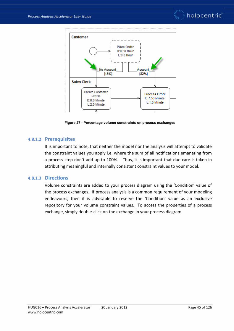
Process Analysis Accelerator User Guide
HUG016 – Process Analysis Accelerator 20 January 2012 Page 45 of 126 www.holocentric.com
Figure 27 - Percentage volume constraints on process exchanges
4.8.1.2 Prerequisites
It is important to note, that neither the model nor the analysis will attempt to validate
the constraint values you apply i.e. where the sum of all notifications emanating from
a process step don’t add up to 100%. Thus, it is important that due care is taken in
attributing meaningful and internally consistent constraint values to your model.
4.8.1.3 Directions
Volume constraints are added to your process diagram using the ‘Condition’ value of
the process exchanges. If process analysis is a common requirement of your modeling
endeavours, then it is advisable to reserve the ‘Condition’ value as an exclusive
repository for your volume constraint values. To access the properties of a process
exchange, simply double-click on the exchange in your process diagram.

Process Analysis Accelerator User Guide
HUG016 – Process Analysis Accelerator 20 January 2012 Page 46 of 126 www.holocentric.com
Figure 28 - Process Exchange Property Dialog
In the ‘Label’ field, succinctly describe the reason or business rule that dictates why
this path would be taken over another. The ‘Label’ serves no real purpose beyond its
visual value on the process diagram, but as such it is very useful device to aid
stakeholders in comprehending the reason behind the branching of a process.
In the ‘Condition’ field enter the average percentage of work (e.g. 82%) that you wish
the process analysis engine to use when performing its analysis. Note: The value you
enter in the ‘Condition’ field must be accompanied by a % symbol.
Work your way through your process model assigning the Label and Condition values
to all relevant exchanges. Obviously, it is not necessary to set a volume constraint if
there is only one exchange (notification) exiting a process step. As you would expect,
the model will assume a throughput of 100% in such circumstances.
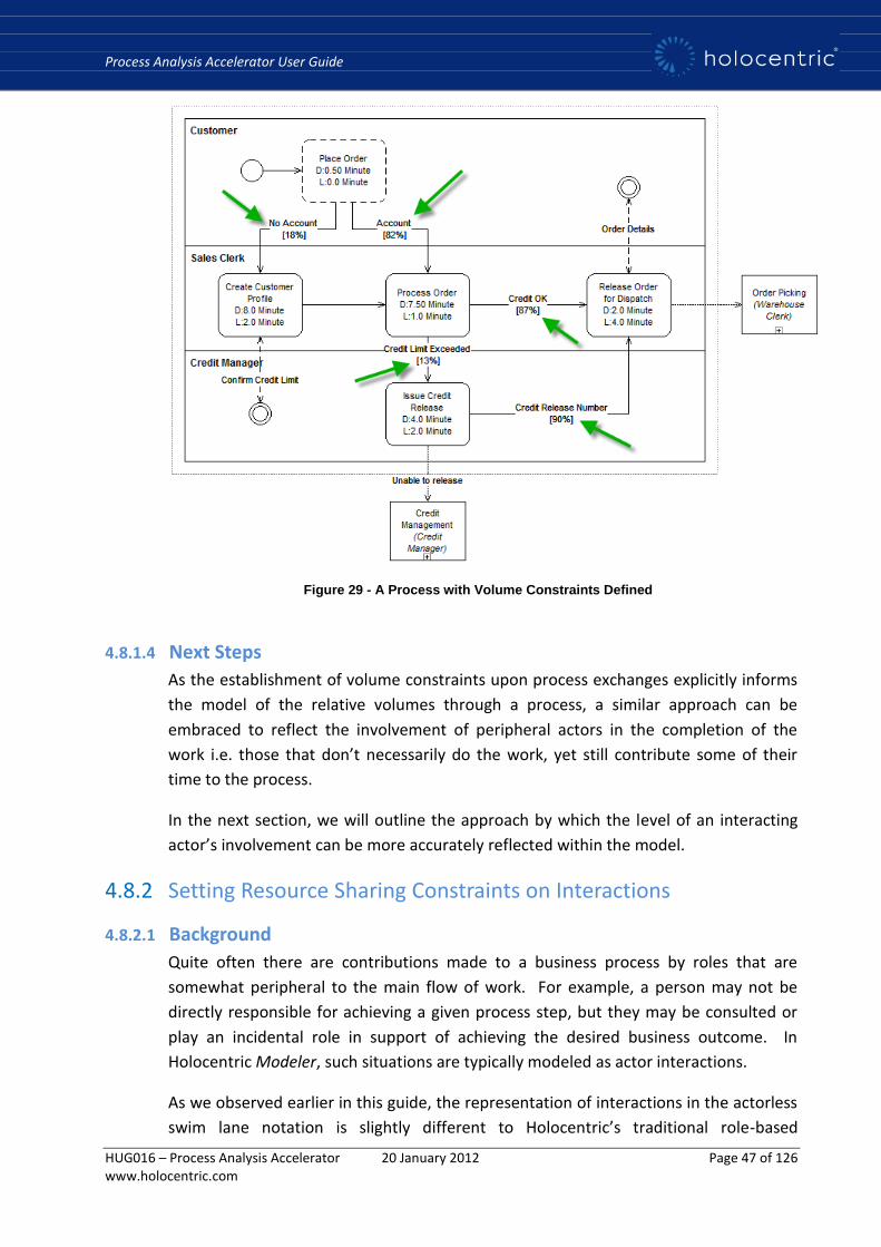
Process Analysis Accelerator User Guide
HUG016 – Process Analysis Accelerator 20 January 2012 Page 47 of 126 www.holocentric.com
Figure 29 - A Process with Volume Constraints Defined
4.8.1.4 Next Steps
As the establishment of volume constraints upon process exchanges explicitly informs
the model of the relative volumes through a process, a similar approach can be
embraced to reflect the involvement of peripheral actors in the completion of the
work i.e. those that don’t necessarily do the work, yet still contribute some of their
time to the process.
In the next section, we will outline the approach by which the level of an interacting
actor’s involvement can be more accurately reflected within the model.
4.8.2 Setting Resource Sharing Constraints on Interactions
4.8.2.1 Background
Quite often there are contributions made to a business process by roles that are
somewhat peripheral to the main flow of work. For example, a person may not be
directly responsible for achieving a given process step, but they may be consulted or
play an incidental role in support of achieving the desired business outcome. In
Holocentric Modeler, such situations are typically modeled as actor interactions.
As we observed earlier in this guide, the representation of interactions in the actorless
swim lane notation is slightly different to Holocentric’s traditional role-based
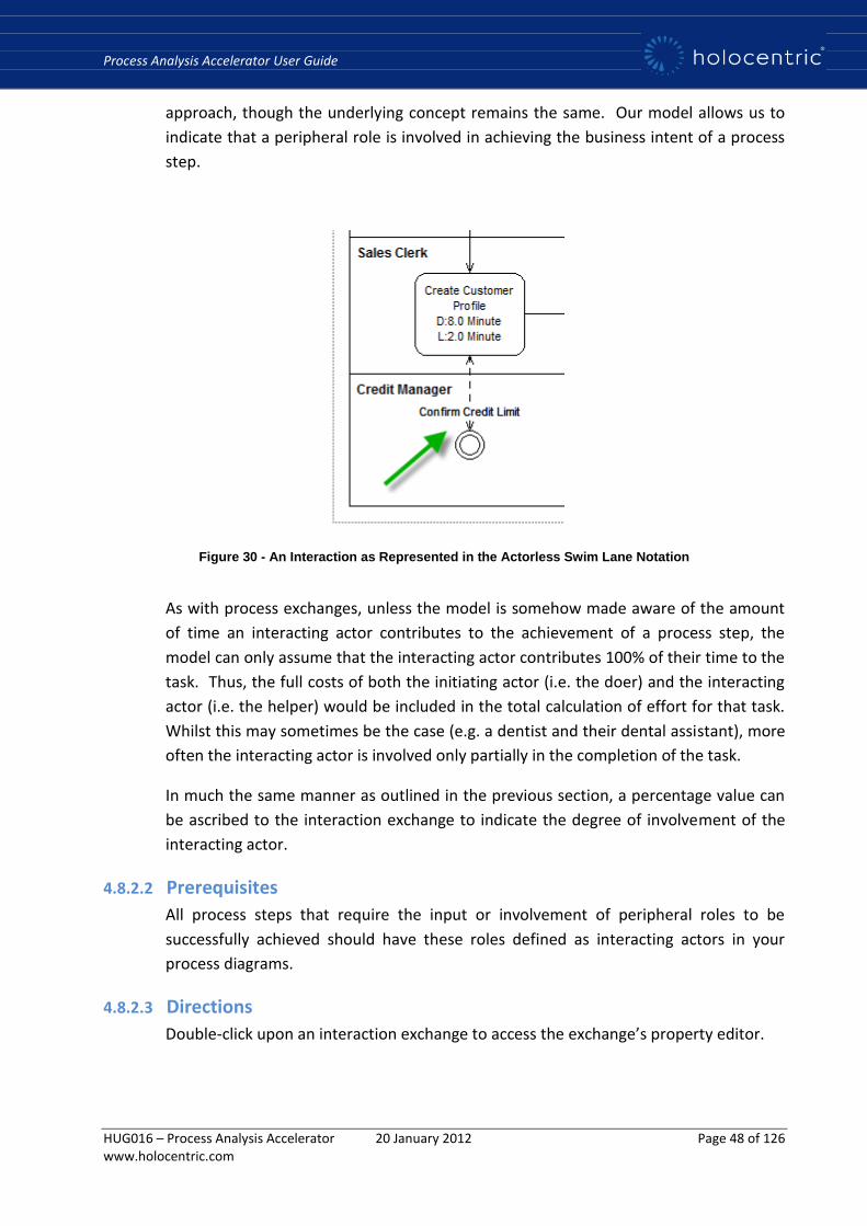
Process Analysis Accelerator User Guide
HUG016 – Process Analysis Accelerator 20 January 2012 Page 48 of 126 www.holocentric.com
approach, though the underlying concept remains the same. Our model allows us to
indicate that a peripheral role is involved in achieving the business intent of a process
step.
Figure 30 - An Interaction as Represented in the Actorless Swim Lane Notation
As with process exchanges, unless the model is somehow made aware of the amount
of time an interacting actor contributes to the achievement of a process step, the
model can only assume that the interacting actor contributes 100% of their time to the
task. Thus, the full costs of both the initiating actor (i.e. the doer) and the interacting
actor (i.e. the helper) would be included in the total calculation of effort for that task.
Whilst this may sometimes be the case (e.g. a dentist and their dental assistant), more
often the interacting actor is involved only partially in the completion of the task.
In much the same manner as outlined in the previous section, a percentage value can
be ascribed to the interaction exchange to indicate the degree of involvement of the
interacting actor.
4.8.2.2 Prerequisites
All process steps that require the input or involvement of peripheral roles to be
successfully achieved should have these roles defined as interacting actors in your
process diagrams.
4.8.2.3 Directions
Double-click upon an interaction exchange to access the exchange’s property editor.
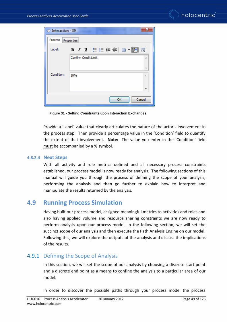
Process Analysis Accelerator User Guide
HUG016 – Process Analysis Accelerator 20 January 2012 Page 49 of 126 www.holocentric.com
Figure 31 - Setting Constraints upon Interaction Exchanges
Provide a ‘Label’ value that clearly articulates the nature of the actor’s involvement in
the process step. Then provide a percentage value in the ‘Condition’ field to quantify
the extent of that involvement. Note: The value you enter in the ‘Condition’ field
must be accompanied by a % symbol.
4.8.2.4 Next Steps
With all activity and role metrics defined and all necessary process constraints
established, our process model is now ready for analysis. The following sections of this
manual will guide you through the process of defining the scope of your analysis,
performing the analysis and then go further to explain how to interpret and
manipulate the results returned by the analysis.
4.9 Running Process Simulation Having built our process model, assigned meaningful metrics to activities and roles and
also having applied volume and resource sharing constraints we are now ready to
perform analysis upon our process model. In the following section, we will set the
succinct scope of our analysis and then execute the Path Analysis Engine on our model.
Following this, we will explore the outputs of the analysis and discuss the implications
of the results.
4.9.1 Defining the Scope of Analysis
In this section, we will set the scope of our analysis by choosing a discrete start point
and a discrete end point as a means to confine the analysis to a particular area of our
model.
In order to discover the possible paths through your process model the process
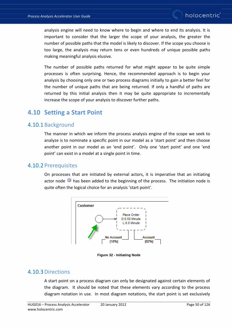
Process Analysis Accelerator User Guide
HUG016 – Process Analysis Accelerator 20 January 2012 Page 50 of 126 www.holocentric.com
analysis engine will need to know where to begin and where to end its analysis. It is
important to consider that the larger the scope of your analysis, the greater the
number of possible paths that the model is likely to discover. If the scope you choose is
too large, the analysis may return tens or even hundreds of unique possible paths
making meaningful analysis elusive.
The number of possible paths returned for what might appear to be quite simple
processes is often surprising. Hence, the recommended approach is to begin your
analysis by choosing only one or two process diagrams initially to gain a better feel for
the number of unique paths that are being returned. If only a handful of paths are
returned by this initial analysis then it may be quite appropriate to incrementally
increase the scope of your analysis to discover further paths.
4.10 Setting a Start Point
4.10.1 Background
The manner in which we inform the process analysis engine of the scope we seek to
analyze is to nominate a specific point in our model as a ‘start point’ and then choose
another point in our model as an ‘end point’. Only one ‘start point’ and one ‘end
point’ can exist in a model at a single point in time.
4.10.2 Prerequisites
On processes that are initiated by external actors, it is imperative that an initiating
actor node has been added to the beginning of the process. The initiation node is
quite often the logical choice for an analysis ‘start point’.
Figure 32 - Initiating Node
4.10.3 Directions
A start point on a process diagram can only be designated against certain elements of
the diagram. It should be noted that these elements vary according to the process
diagram notation in use. In most diagram notations, the start point is set exclusively
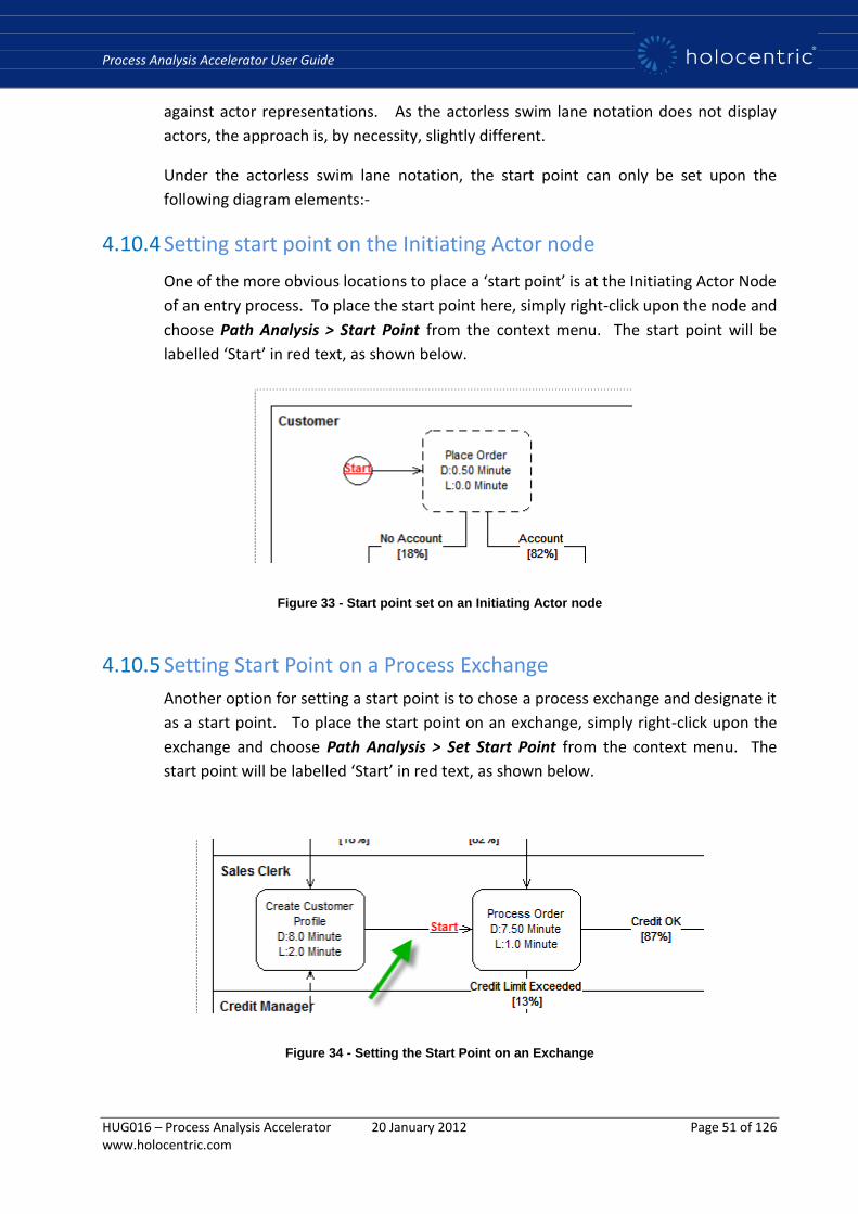
Process Analysis Accelerator User Guide
HUG016 – Process Analysis Accelerator 20 January 2012 Page 51 of 126 www.holocentric.com
against actor representations. As the actorless swim lane notation does not display
actors, the approach is, by necessity, slightly different.
Under the actorless swim lane notation, the start point can only be set upon the
following diagram elements:-
4.10.4 Setting start point on the Initiating Actor node
One of the more obvious locations to place a ‘start point’ is at the Initiating Actor Node
of an entry process. To place the start point here, simply right-click upon the node and
choose Path Analysis > Start Point from the context menu. The start point will be
labelled ‘Start’ in red text, as shown below.
Figure 33 - Start point set on an Initiating Actor node
4.10.5 Setting Start Point on a Process Exchange
Another option for setting a start point is to chose a process exchange and designate it
as a start point. To place the start point on an exchange, simply right-click upon the
exchange and choose Path Analysis > Set Start Point from the context menu. The
start point will be labelled ‘Start’ in red text, as shown below.
Figure 34 - Setting the Start Point on an Exchange
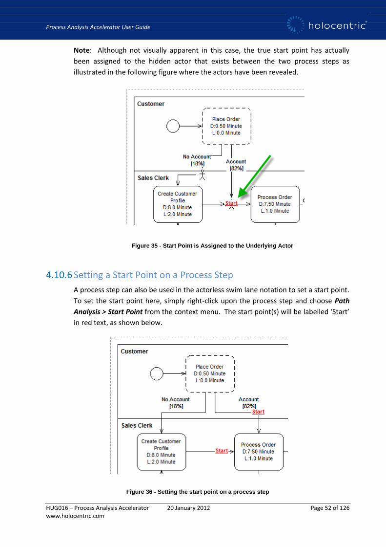
Process Analysis Accelerator User Guide
HUG016 – Process Analysis Accelerator 20 January 2012 Page 52 of 126 www.holocentric.com
Note: Although not visually apparent in this case, the true start point has actually
been assigned to the hidden actor that exists between the two process steps as
illustrated in the following figure where the actors have been revealed.
4.10.6 Setting a Start Point on a Process Step
A process step can also be used in the actorless swim lane notation to set a start point.
To set the start point here, simply right-click upon the process step and choose Path
Analysis > Start Point from the context menu. The start point(s) will be labelled ‘Start’
in red text, as shown below.
Figure 36 - Setting the start point on a process step
Figure 35 - Start Point is Assigned to the Underlying Actor

Process Analysis Accelerator User Guide
HUG016 – Process Analysis Accelerator 20 January 2012 Page 53 of 126 www.holocentric.com
Note: Even though it would appear that two start points have been created using this
approach, the start point has again been assigned to the underlying actor as shown in
the previous figure. Structurally, the two inbound paths actually converge at the actor
preceding the process step. Hence, there is really only one start point, but in the
actorless view, a ‘Start’ label will be displayed on all inbound exchanges to highlight to
the user that the chosen process step will fall within scope of the analysis.
Should you need to remove a start point from a process diagram at any time, right-
click anywhere on the diagram canvas and choose Path Analysis > Clear Start & End
Point from the context menu.
4.10.7 Next Steps
With a start point defined, we will now take a similar approach to setting an end point
as will be covered in the next section.
4.11 Setting an End Point
4.11.1 Background
In much the same manner as we set a ‘start point’ for the analysis, we can also set an
‘end point’. As with the start point, there are again some subtle variations in approach
between the standard diagram notations in Holocentric and the Process Analysis
Accelerator’s actorless swim lane notation. Whilst these variations will be covered in
more detail in Appendix 1, the primary difference of course is the absence of actor
representations in the actorless view.
4.11.2 Prerequisites
You need to ensure that there is at least one process step that occurs between the
nominated ‘start’ and ‘end’ points of your process.
4.11.3 Directions
An end point on a process diagram can only be designated against certain elements of
the diagram. It should be noted that these elements vary according to the process
diagram notation in use. In most diagram notations, the end point is set exclusively
against actor representations. As the actorless swim lane notation does not display
actors, the approach is, by necessity, slightly different.
Under the actorless swim lane notation, the end point can only be set upon the
following diagram elements:
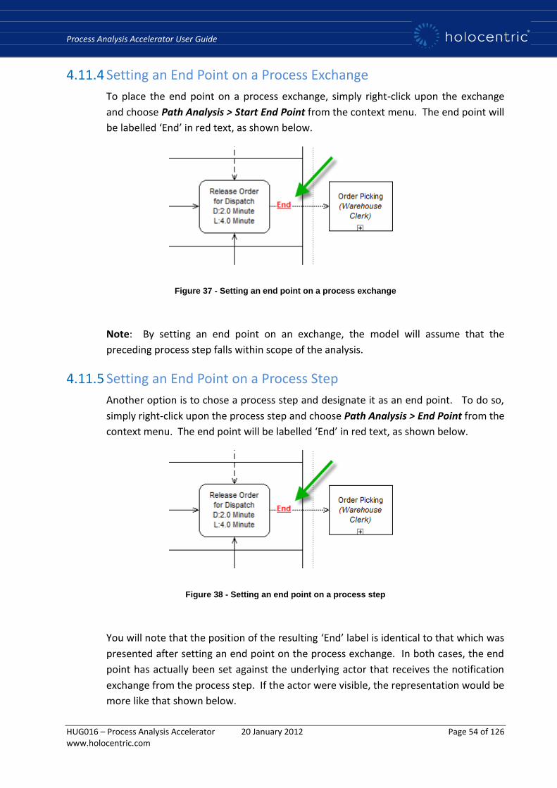
Process Analysis Accelerator User Guide
HUG016 – Process Analysis Accelerator 20 January 2012 Page 54 of 126 www.holocentric.com
4.11.4 Setting an End Point on a Process Exchange
To place the end point on a process exchange, simply right-click upon the exchange
and choose Path Analysis > Start End Point from the context menu. The end point will
be labelled ‘End’ in red text, as shown below.
Figure 37 - Setting an end point on a process exchange
Note: By setting an end point on an exchange, the model will assume that the
preceding process step falls within scope of the analysis.
4.11.5 Setting an End Point on a Process Step
Another option is to chose a process step and designate it as an end point. To do so,
simply right-click upon the process step and choose Path Analysis > End Point from the
context menu. The end point will be labelled ‘End’ in red text, as shown below.
Figure 38 - Setting an end point on a process step
You will note that the position of the resulting ‘End’ label is identical to that which was
presented after setting an end point on the process exchange. In both cases, the end
point has actually been set against the underlying actor that receives the notification
exchange from the process step. If the actor were visible, the representation would be
more like that shown below.

Process Analysis Accelerator User Guide
HUG016 – Process Analysis Accelerator 20 January 2012 Page 55 of 126 www.holocentric.com
Figure 39 - End point with actor underlying actor shown
Should you need to remove an end point from a process diagram at any time, right-
click anywhere on the diagram canvas and choose Path Analysis > Clear Start & End
Point from the context menu.
4.11.6 Next Steps
The scope of our analysis is now clearly defined through the addition of a start and end
point to our model. In the following section we will invoke the process analysis engine
and review the results of our analysis.
Process Analysis Accelerator User Guide
HUG016 – Process Analysis Accelerator 20 January 2012 Page 56 of 126 www.holocentric.com
5 Performing Path Analysis In this section we will outline the method to configure the path analysis Excel template
to define new default values, such as the default number of shifts per year and the
default number of hours per shift. Following this, we will describe how to launch the
process analysis simulation engine and discuss the generation of the Excel Path
Analysis spreadsheet. Finally, will describe how to perform ad hoc process analysis by
launching the Excel spreadsheet manually, with the option to override certain default
values at run time.
5.1 Set Excel Model Default Parameters
5.1.1 Background
Even though much of the analytical data that the path analysis spreadsheet presents is
sourced directly from the XML file itself, there are also a number of default parameters
contained within the spreadsheet and applied at the time the XML simulation file is
loaded. These parameters contribute directly to the spreadsheet’s calculations. Some
examples of the default parameters are the standard number of shifts per annum and
the standard hours per shift.
Whilst it is possible to perform analysis manually and to substitute some parameters at
run time (e.g. Shifts and Hours), if these parameters always need to be substituted, it
may be more practical to set alternative default parameters to apply for all future
analysis. This outcome can be achieved by making changes to the MS Excel path
analysis template file.
If the template has been updated and saved, the new values that you have set for the
template will subsequently be applied to all future path analysis results.
The following parameters can be updated in the Excel template:
The default file path for the XML input file
The default simulation type
The number of simulations before a new file is created
The default number of shifts per annum
Number of working hours per shift
Whilst all of these parameters can be modified, it is generally recommended that
changes to the template be confined predominantly to the ‘shifts’ and ‘working hours’
values, as changing the other parameters may affect the performance and integrity of

Process Analysis Accelerator User Guide
HUG016 – Process Analysis Accelerator 20 January 2012 Page 57 of 126 www.holocentric.com
your analysis. Note: Changing the default file path would only be necessary if you
were seeking to load XML files from an alternative location to the current default of
My Documents/Path Analysis.
5.1.2 Prerequisites
Important: If you are content with the current default values that are being applied to
your analysis, then there is no need for you to modify the default template.
If you do seek to update the template, then you will need read/write permission for
the directory where Modeler is installed (e.g. C:/Program Files).
It is also advisable to take a back up copy of the template to allow easy recovery if the
changes you make appear to cause adverse affects upon your analysis.
5.1.3 Directions
Locate the file XMLImport Base.xls within the Holocentric install directory e.g.
C:\Program Files\Holocentric\Modeler\Data\Templates\Path Analysis (i.e. where
Modeler has been installed to C:\Program Files).
Take a copy of the file as a back up and then open the XMLImport Base.xls template
file by double-clicking upon it.
Excel should prompt you with a security notice indicating the presence of macros in
the template file. You must choose Enable Macros to proceed.
Figure 40 - Microsoft Security Notice
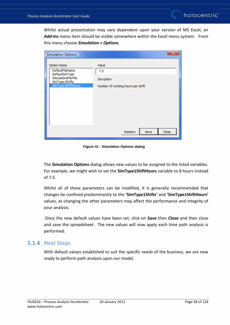
Process Analysis Accelerator User Guide
HUG016 – Process Analysis Accelerator 20 January 2012 Page 58 of 126 www.holocentric.com
Whilst actual presentation may vary dependent upon your version of MS Excel, an
Add-Ins menu item should be visible somewhere within the Excel menu system. From
this menu choose Simulation > Options.
Figure 41 - Simulation Options dialog
The Simulation Options dialog allows new values to be assigned to the listed variables.
For example, we might wish to set the SimType1ShiftHours variable to 8 hours instead
of 7.5.
Whilst all of these parameters can be modified, it is generally recommended that
changes be confined predominantly to the ‘SimType1Shifts’ and ‘SimType1ShiftHours’
values, as changing the other parameters may affect the performance and integrity of
your analysis.
Once the new default values have been set, click on Save then Close and then close
and save the spreadsheet. The new values will now apply each time path analysis is
performed.
5.1.4 Next Steps
With default values established to suit the specific needs of the business, we are now
ready to perform path analysis upon our model.

Process Analysis Accelerator User Guide
HUG016 – Process Analysis Accelerator 20 January 2012 Page 59 of 126 www.holocentric.com
5.2 Finding Paths
5.2.1 Background
The Simulation Engine can now be invoked upon your model. The analysis will attempt
to discover all possible paths between your nominated Start and End points. The
number of paths found by the Simulation will of course depend on the complexity of
your model, along with the positions of your chosen Start and End points.
When it has finished traversing the business model, it will generate an output file and
then launch a Microsoft Excel® spreadsheet to display the results. The Path Analysis
spreadsheet is designed to present an analysis of the total costs and time between the
Start and End points for all of the paths found, over the course of a period of time.
In order to do this, the path analysis spreadsheet will use the following inputs from
your model:
The time period over which the Paths will be analyzed.
The annual cost associated with each Process Role.
How many people in the business are playing the Process Role.
How long each process step takes to complete.
How long after a process step is completed before the next process step can
commence.
How many times in a day the process step occurs.
How frequently each particular path occurs, with respect to all of the possible
paths discovered.
The values for some of these come directly from your business model, and are written
to the output file. If, however, the information has not been specified in your business
model, Modeler will assign some default values to maintain spreadsheet integrity (e.g.
to prevent ‘divide by 0’ errors).
The spreadsheet then allows you to manipulate a range of parameters so that you can
compare a set of hypothetical values to those assigned to your model (i.e. to perform
‘what-if’ analysis).
5.2.2 Prerequisites
In preparation for running a process simulation upon your model, you should ensure
that at least the following requirements have been satisfied:
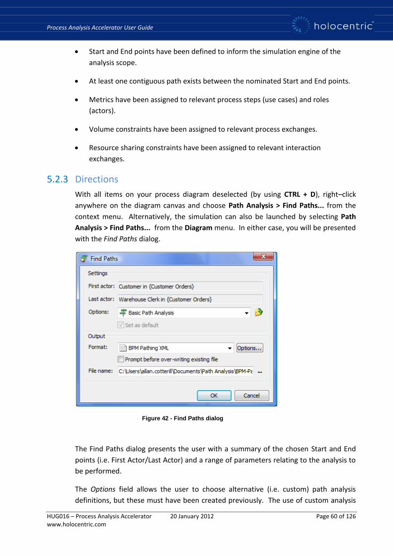
Process Analysis Accelerator User Guide
HUG016 – Process Analysis Accelerator 20 January 2012 Page 60 of 126 www.holocentric.com
Start and End points have been defined to inform the simulation engine of the
analysis scope.
At least one contiguous path exists between the nominated Start and End points.
Metrics have been assigned to relevant process steps (use cases) and roles
(actors).
Volume constraints have been assigned to relevant process exchanges.
Resource sharing constraints have been assigned to relevant interaction
exchanges.
5.2.3 Directions
With all items on your process diagram deselected (by using CTRL + D), right–click
anywhere on the diagram canvas and choose Path Analysis > Find Paths... from the
context menu. Alternatively, the simulation can also be launched by selecting Path
Analysis > Find Paths... from the Diagram menu. In either case, you will be presented
with the Find Paths dialog.
Figure 42 - Find Paths dialog
The Find Paths dialog presents the user with a summary of the chosen Start and End
points (i.e. First Actor/Last Actor) and a range of parameters relating to the analysis to
be performed.
The Options field allows the user to choose alternative (i.e. custom) path analysis
definitions, but these must have been created previously. The use of custom analysis

Process Analysis Accelerator User Guide
HUG016 – Process Analysis Accelerator 20 January 2012 Page 61 of 126 www.holocentric.com
definitions typically applies to advanced scenario based simulation which will be
covered later in this user guide. For standard simulations, always leave this field at its
default value of ‘Basic Path Analysis’.
In the Output section of the dialog are a number of fields relating to the nature and
save destination of the XML output file. At this stage only the ‘BPM Pathing XML’
format is supported, so again, leave the Format field unchanged at its default value.
Only use the ‘Prompt before over-writing existing file’ check box if you would prefer to
be prompted every time you run the analysis to save over the last simulation file that
was generated. If left unchecked (the default), Modeler will always generate a file of
the same name to the same location, overwriting the previous file each time. Note:
This refers to the XML path analysis output file, not the resulting Excel spreadsheet.
Unless the File name field is modified, a new Path Analysis folder will be created under
My Documents (or Documents - if using Vista) the first time an analysis is run.
Subsequently, the XML output file will be generated to this folder each time a
simulation is run.
Clicking upon the OK button will invoke the simulation engine and it will commence its
analysis. The mouse pointer should indicate that analysis is occurring in the
background and Microsoft Excel® will open automatically. The result of the path
analysis will then be compiled and presented within the Path Analysis spreadsheet.
Figure 43 - Path Analysis Spreadsheet - Dashboard
Process Analysis Accelerator User Guide
HUG016 – Process Analysis Accelerator 20 January 2012 Page 62 of 126 www.holocentric.com
5.2.4 Next Steps
Whenever Modeler’s basic process simulation is performed, there are a range of
standard values and parameters that are applied to the spreadsheet. Included among
these values, for example, is a value for the standard number of shifts per annum (232)
and another for the standard number of hours per shift (7.5). As all businesses vary in
respect to the days and hours worked, it may sometimes be advantageous to use
different input values for a simulation.
The following section will outline the means by which the Basic Path Analysis
spreadsheet can be launched manually, either from within Modeler or independently
of Modeler, and how certain parameters can be modified to influence that nature of
the simulation.
5.3 Launching the Excel Model Manually
5.3.1 Background
As we learned previously, there are a range of parameters contained within the Excel
template which are applied by default to all simulations generated from within
Modeler. It was also revealed that it is possible to modify the path analysis Excel
template to set new default values for these parameters.
Whilst the above approach is very useful for defining new default values for all future
analysis, there may still be occasions when alternate values need to be used to
perform ad hoc analysis e.g. testing ‘what-if’ scenarios.
To support ad hoc analysis of this nature, it is possible to launch the Excel spreadsheet
independently of Modeler and to manually override certain default values as the
spreadsheet loads. As a result, the newly provided values will be used by the
spreadsheet in its calculations and applied to the path analysis data.

Process Analysis Accelerator User Guide
HUG016 – Process Analysis Accelerator 20 January 2012 Page 63 of 126 www.holocentric.com
5.3.2 Prerequisites
To launch the Excel spreadsheet manually and to load an analysis file, you must have
performed a recent analysis of your model so that a current XML data file is available
to be loaded by the spreadsheet.
To have visibility of the Add-Ins menu, you must first have your Excel security settings
set to Enable Macros. Please refer to MS Excel help files if you are unsure how to
enable macros.
5.3.3 Directions
Launching the spreadsheet
There are two methods of launching the spreadsheet manually. One method entails
launching the spreadsheet from within Modeler’s menu structure, the other from
within an existing path analysis spreadsheet in Excel.
To open the spreadsheet manually from within Modeler, access the Tools menu and
choose Process Analysis > Path Review > Show Excel Model. Once the template file
has opened, choose Simulation > Run Simulation from the Add-Ins menu*.
To open the spreadsheet manually from within an existing path analysis spreadsheet,
choose Simulation > Run Simulation from the Add-Ins menu*.
* Note: To have visibility of the Add-Ins menu, you must first have your Excel security
settings set to Enable Macros. Please refer to MS Excel help files if you are unsure
how to enable macros.
In either case, the Run Simulation dialog will be presented showing the options that
can be modified to influence your analysis.
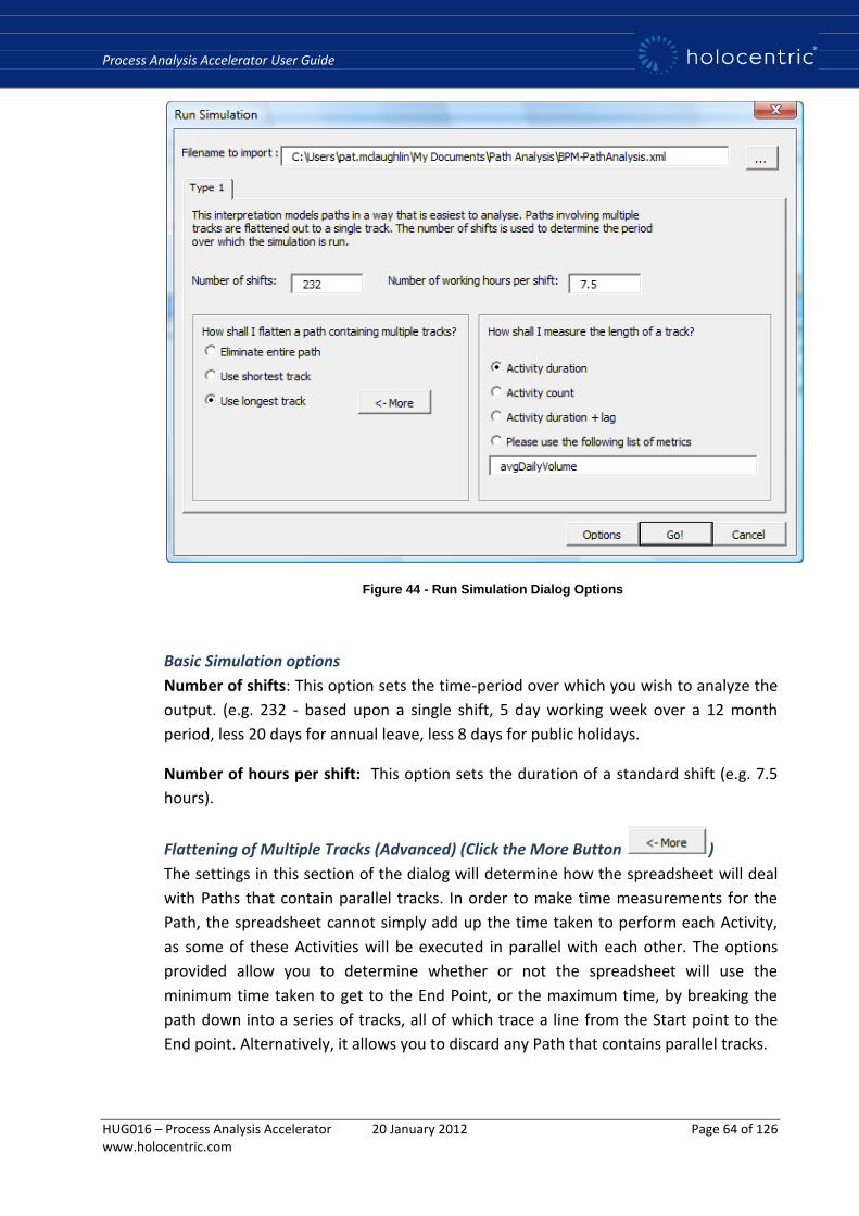
Process Analysis Accelerator User Guide
HUG016 – Process Analysis Accelerator 20 January 2012 Page 64 of 126 www.holocentric.com
Figure 44 - Run Simulation Dialog Options
Basic Simulation options
Number of shifts: This option sets the time-period over which you wish to analyze the
output. (e.g. 232 - based upon a single shift, 5 day working week over a 12 month
period, less 20 days for annual leave, less 8 days for public holidays.
Number of hours per shift: This option sets the duration of a standard shift (e.g. 7.5
hours).
Flattening of Multiple Tracks (Advanced) (Click the More Button )
The settings in this section of the dialog will determine how the spreadsheet will deal
with Paths that contain parallel tracks. In order to make time measurements for the
Path, the spreadsheet cannot simply add up the time taken to perform each Activity,
as some of these Activities will be executed in parallel with each other. The options
provided allow you to determine whether or not the spreadsheet will use the
minimum time taken to get to the End Point, or the maximum time, by breaking the
path down into a series of tracks, all of which trace a line from the Start point to the
End point. Alternatively, it allows you to discard any Path that contains parallel tracks.
Process Analysis Accelerator User Guide
HUG016 – Process Analysis Accelerator 20 January 2012 Page 65 of 126 www.holocentric.com
Remove consequential items: This is on by default. The spreadsheet will prune off all
items that are included in the output as a result of the ‘Show Consequences’ option in
Modeler being set to true. If you uncheck this option, then your results will include ALL
of the Activities that are exported from Modeler, without any kind of filtering.
Remove identical paths: This option is only meaningful when you are also removing
consequential items, above. As a result of removing consequences, you might be left
with a collection of paths that all look the same as each other. (Their only differences
were contained in the items that were pruned off). If you check this option, (and it is
on by default), the spreadsheet will do a study of all of the Paths in the filtered output,
and eliminate all Paths that look the same as others, in terms of their sequencing, and
the values of their metric.
Items on the selected track only: When a path is flattened according to the options
you have specified (above), you can tell the spreadsheet to eliminate all results except
for those items that appear on the flattened track chosen according to the options,
even if some of those tracks ended up reaching the Finishing Point.
Remove unsuccessful paths: Modeler is capable of providing a complete description of
all of the traversals it has made, including all of the dead ends where it was unable to
reach the designated Last Actor. If this option is checked, (it is on by default), the
spreadsheet will eliminate those items that do not lie on successful Paths, when
filtering the results.
Measuring the length of a track (Advanced)
Further to the flattening of Paths which contain parallel tracks, the spreadsheet also
allows you to determine how the length of a track will be measured. Modeler has a
collection of predefined Activity Business- Metrics, which are included in the output by
default. You can choose how these will be used:
Activity Duration: This option will use an aggregation of the time taken to perform the
Activities for all of the Activities contained in a track.
Activity Count: This option simply uses the number of Activities appearing in the track
as a direct measure of its length.
Activity Duration + lag: This option will measure a track length based on an aggregation
of time taken to perform the Activities, as well as the Activity-Lag time. This lag time is
a representation of the time usually taken before an Activity will commence. (For
example, performing an Activity might only take half a day, but it sits on a desk for
more that 2 days before it is processed).
Custom list of metrics: This allows you to provide a comma-separated list of the
metrics that it will measure and aggregate for all Activities, Actors, and Edges that
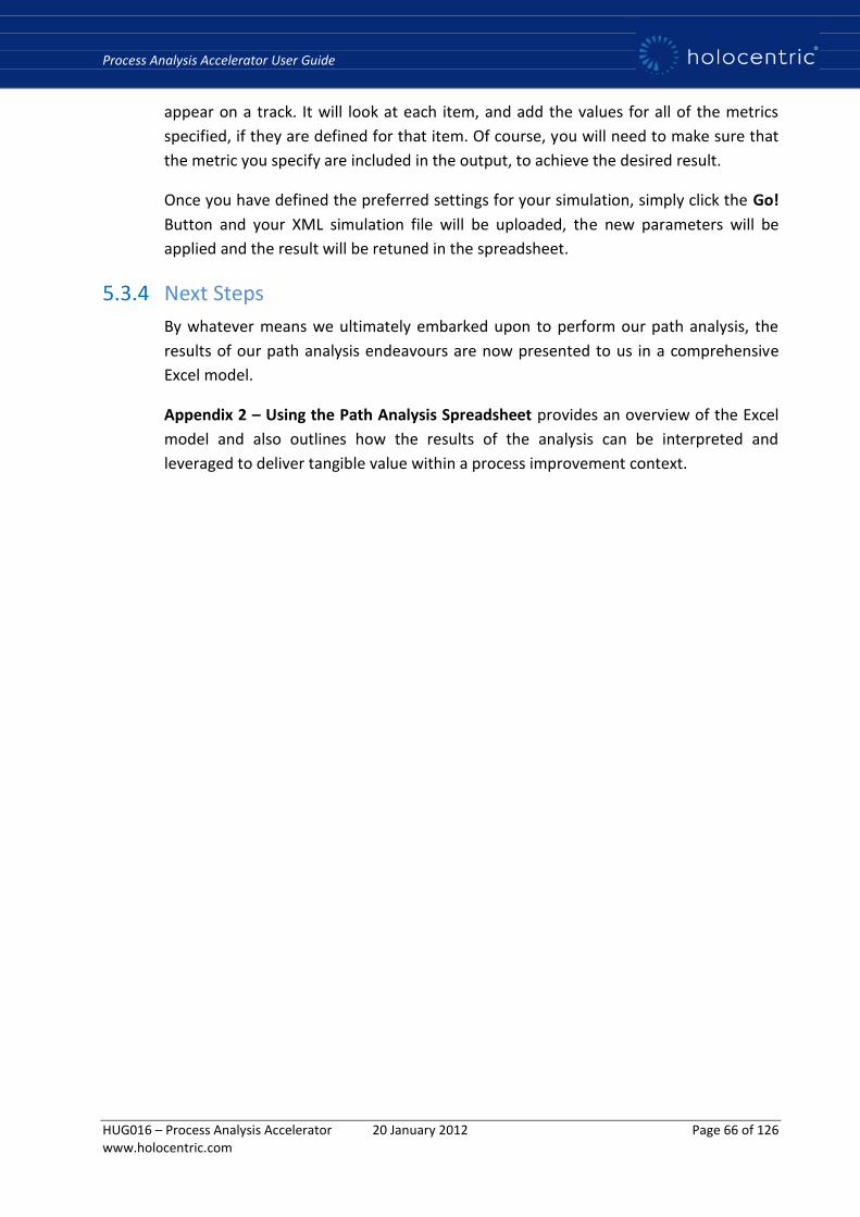
Process Analysis Accelerator User Guide
HUG016 – Process Analysis Accelerator 20 January 2012 Page 66 of 126 www.holocentric.com
appear on a track. It will look at each item, and add the values for all of the metrics
specified, if they are defined for that item. Of course, you will need to make sure that
the metric you specify are included in the output, to achieve the desired result.
Once you have defined the preferred settings for your simulation, simply click the Go!
Button and your XML simulation file will be uploaded, the new parameters will be
applied and the result will be retuned in the spreadsheet.
5.3.4 Next Steps
By whatever means we ultimately embarked upon to perform our path analysis, the
results of our path analysis endeavours are now presented to us in a comprehensive
Excel model.
Appendix 2 – Using the Path Analysis Spreadsheet provides an overview of the Excel
model and also outlines how the results of the analysis can be interpreted and
leveraged to deliver tangible value within a process improvement context.
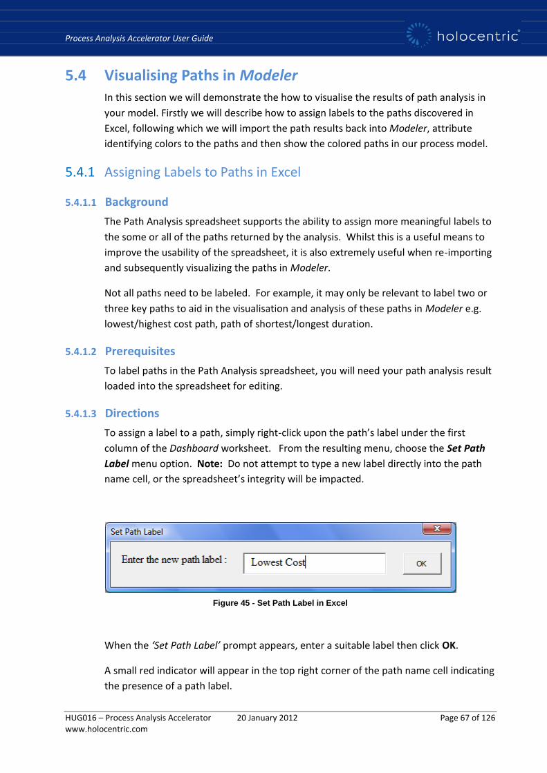
Process Analysis Accelerator User Guide
HUG016 – Process Analysis Accelerator 20 January 2012 Page 67 of 126 www.holocentric.com
5.4 Visualising Paths in Modeler In this section we will demonstrate the how to visualise the results of path analysis in
your model. Firstly we will describe how to assign labels to the paths discovered in
Excel, following which we will import the path results back into Modeler, attribute
identifying colors to the paths and then show the colored paths in our process model.
5.4.1 Assigning Labels to Paths in Excel
5.4.1.1 Background
The Path Analysis spreadsheet supports the ability to assign more meaningful labels to
the some or all of the paths returned by the analysis. Whilst this is a useful means to
improve the usability of the spreadsheet, it is also extremely useful when re-importing
and subsequently visualizing the paths in Modeler.
Not all paths need to be labeled. For example, it may only be relevant to label two or
three key paths to aid in the visualisation and analysis of these paths in Modeler e.g.
lowest/highest cost path, path of shortest/longest duration.
5.4.1.2 Prerequisites
To label paths in the Path Analysis spreadsheet, you will need your path analysis result
loaded into the spreadsheet for editing.
5.4.1.3 Directions
To assign a label to a path, simply right-click upon the path’s label under the first
column of the Dashboard worksheet. From the resulting menu, choose the Set Path
Label menu option. Note: Do not attempt to type a new label directly into the path
name cell, or the spreadsheet’s integrity will be impacted.
Figure 45 - Set Path Label in Excel
When the ‘Set Path Label’ prompt appears, enter a suitable label then click OK.
A small red indicator will appear in the top right corner of the path name cell indicating
the presence of a path label.
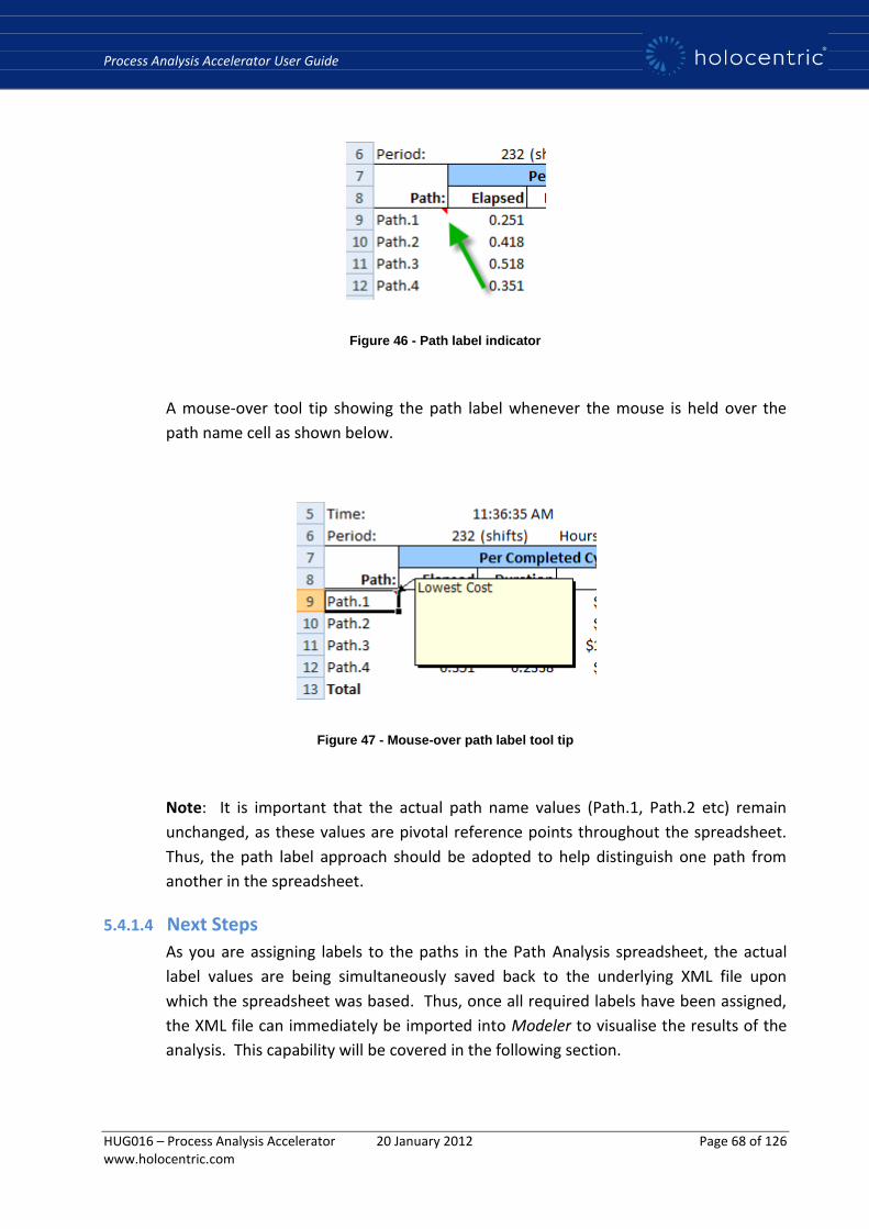
Process Analysis Accelerator User Guide
HUG016 – Process Analysis Accelerator 20 January 2012 Page 68 of 126 www.holocentric.com
Figure 46 - Path label indicator
A mouse-over tool tip showing the path label whenever the mouse is held over the
path name cell as shown below.
Figure 47 - Mouse-over path label tool tip
Note: It is important that the actual path name values (Path.1, Path.2 etc) remain
unchanged, as these values are pivotal reference points throughout the spreadsheet.
Thus, the path label approach should be adopted to help distinguish one path from
another in the spreadsheet.
5.4.1.4 Next Steps
As you are assigning labels to the paths in the Path Analysis spreadsheet, the actual
label values are being simultaneously saved back to the underlying XML file upon
which the spreadsheet was based. Thus, once all required labels have been assigned,
the XML file can immediately be imported into Modeler to visualise the results of the
analysis. This capability will be covered in the following section.
Process Analysis Accelerator User Guide
HUG016 – Process Analysis Accelerator 20 January 2012 Page 69 of 126 www.holocentric.com
5.4.2 Showing Paths
5.4.2.1 Background
Once a simulation has been executed it is then possible to visually display one, some or
all of the discovered paths, in user defined colors upon the relevant diagram(s) of your
model. This capability can prove very useful for reviewing the results of path analysis
in a highly visual manner to gain a better understanding of the results. For example,
the analysis may reveal a number of unexpected paths which can subsequently be
explored in greater detail using the process model.
5.4.2.2 Prerequisites
As the path visualisation functionality utilises the XML path analysis file as its primary
input, at least one path analysis must have been performed on the current model for
this file to exist.
Whilst not essential, it is also desirable that the previously discovered paths have had
meaningful path labels assigned in the Path Analysis spreadsheet (refer previous
section). Not all paths require labels, but it does make the task of distinguishing
between (the potentially numerous) paths so much easier when compared to relying
solely upon the default path names (e.g. Path.1, Path.2 etc).
5.4.3 Directions
From the Tools menu, choose Process Analysis > Path Review > Show Paths... This
menu option will present the first page of the Path Analysis Wizard.
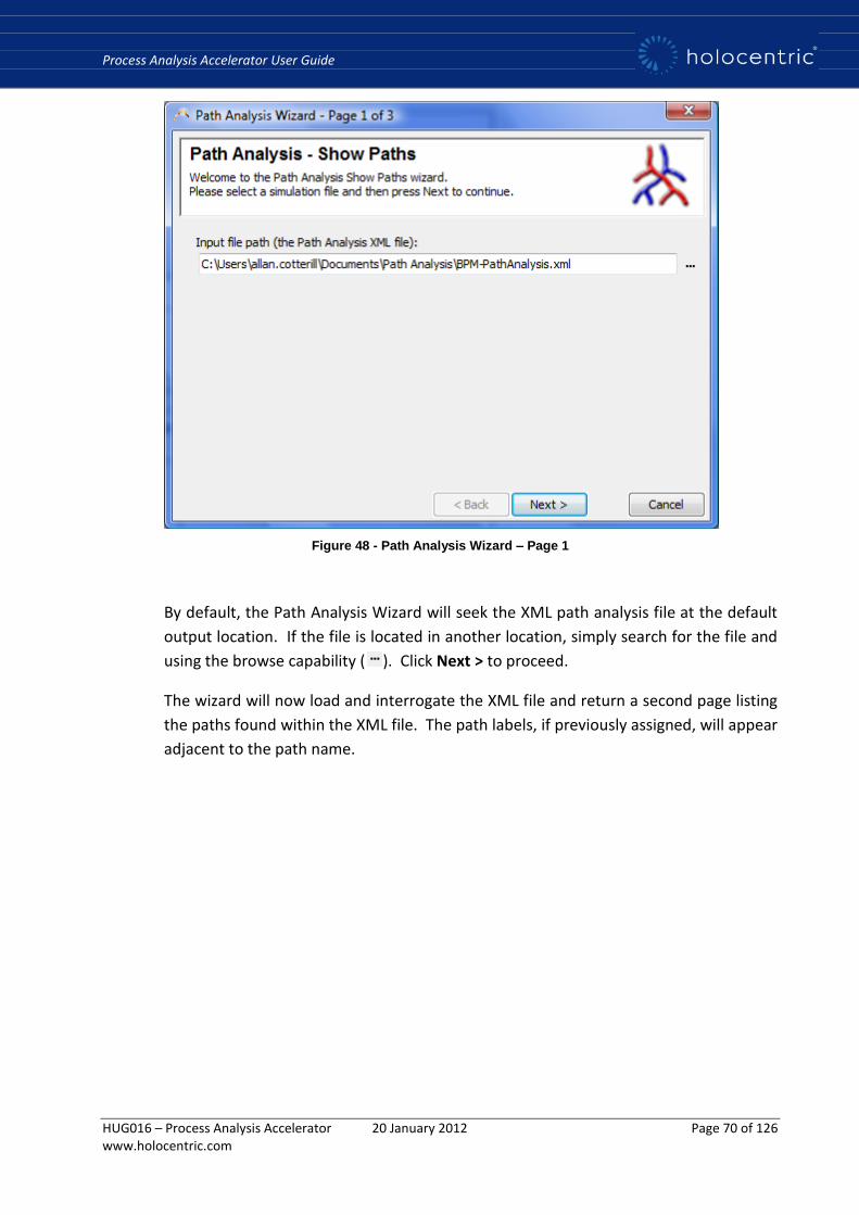
Process Analysis Accelerator User Guide
HUG016 – Process Analysis Accelerator 20 January 2012 Page 70 of 126 www.holocentric.com
Figure 48 - Path Analysis Wizard – Page 1
By default, the Path Analysis Wizard will seek the XML path analysis file at the default
output location. If the file is located in another location, simply search for the file and
using the browse capability ( ). Click Next > to proceed.
The wizard will now load and interrogate the XML file and return a second page listing
the paths found within the XML file. The path labels, if previously assigned, will appear
adjacent to the path name.
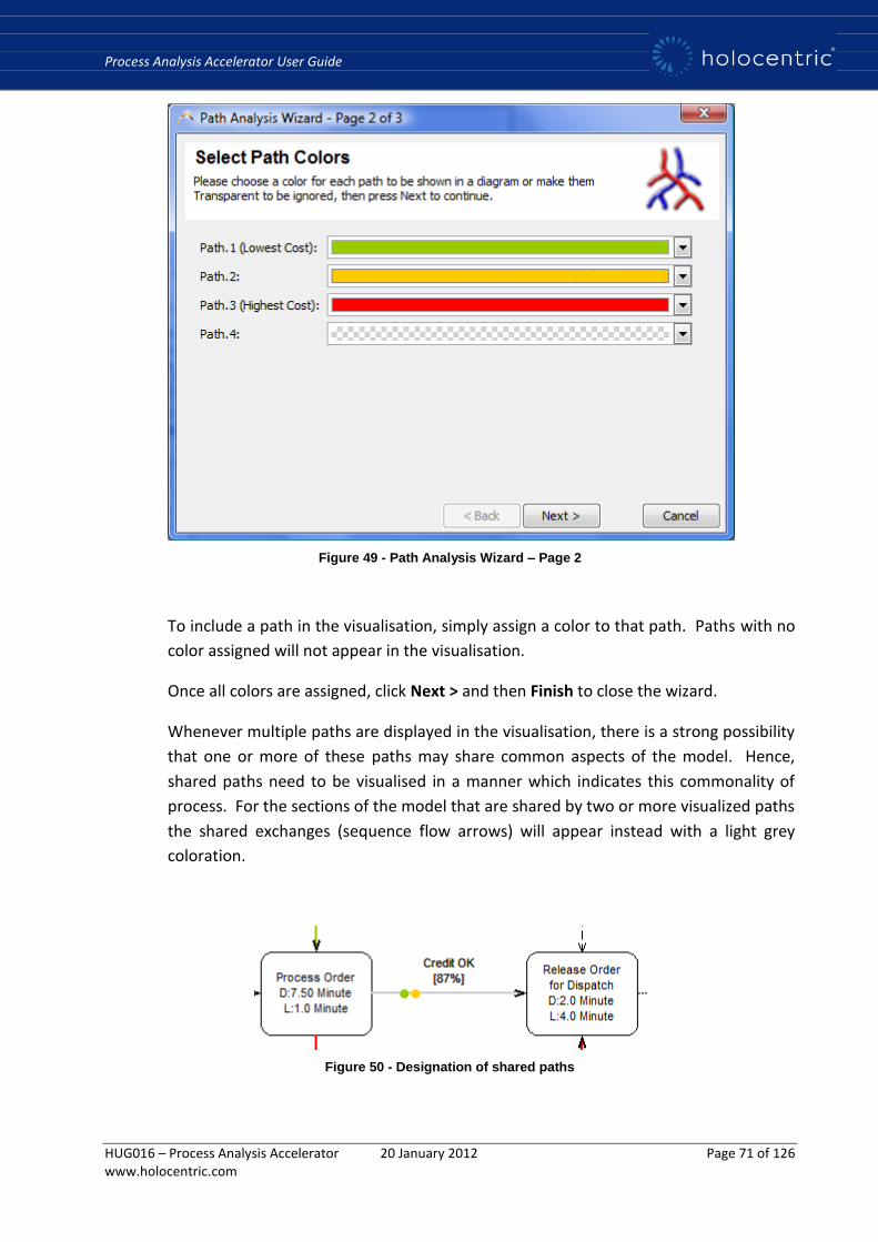
Process Analysis Accelerator User Guide
HUG016 – Process Analysis Accelerator 20 January 2012 Page 71 of 126 www.holocentric.com
Figure 49 - Path Analysis Wizard – Page 2
To include a path in the visualisation, simply assign a color to that path. Paths with no
color assigned will not appear in the visualisation.
Once all colors are assigned, click Next > and then Finish to close the wizard.
Whenever multiple paths are displayed in the visualisation, there is a strong possibility
that one or more of these paths may share common aspects of the model. Hence,
shared paths need to be visualised in a manner which indicates this commonality of
process. For the sections of the model that are shared by two or more visualized paths
the shared exchanges (sequence flow arrows) will appear instead with a light grey
coloration.
Figure 50 - Designation of shared paths
Process Analysis Accelerator User Guide
HUG016 – Process Analysis Accelerator 20 January 2012 Page 72 of 126 www.holocentric.com
In addition, shared exchanges will also be accompanied by a series of indicator icons
that highlight which of the visualised paths share the exchange.
Path visualisation can be executed as many times as you desire e.g. one path at a time
but as cumulative visualisations can become quite messy, it is probably advisable to
clear the previous visualisations in between times by selecting Path Analysis > Path
Review > Hide Paths from the Tools menu.
5.4.4 Next Steps
Up to this point, we have not placed any real constraint upon our analysis in respect to
the number of possible paths that the simulation may discover and return in the
process analysis result.
In this context, our analysis would traverse the entire model and return every possible
unique path that it can identify between the Start and End points. This ‘open slather’
approach can prove very resource intensive, particularly when working with large,
complex models, and can often return voluminous results that become increasingly
difficult to transform into tangible business value.
In some circumstances, you may know exactly which path or paths you wish to
analyze, and hence, running an analysis across the entire model in these situations
would prove an unnecessary waste of time and resources.
In the next section we introduce the concept of Scenarios as a means to tightly
constrain your analysis to include only one (or a few) discrete paths.
Scenarios allow the user to manually plot an explicit journey through the model by
defining inbound and/or outbound conditions or gateways at key nodes along the
process path. Later, when process analysis is invoked on the model, only the paths
conforming to the defined scenario(s) will be evaluated and returned in the result.
Process Analysis Accelerator User Guide
HUG016 – Process Analysis Accelerator 20 January 2012 Page 73 of 126 www.holocentric.com
6 Constraining Path Analysis using Scenarios Left unconstrained, the Path Analysis Engine will attempt to discover every possible
path in a process model between the nominated start and end points. This may not
always be a desirable outcome. For example, the focus of your process improvement
efforts may relate to a very specific aspect of your business process model. Thus, you
may only be interested in analysing one, two or a small handful of paths as opposed to
analysing every possible path every time. Having all possible paths returned in your
analysis every time you run it may make the results of your analysis unnecessarily
complex and unwieldy, thus reducing its value as a process improvement tool.
In this section we introduce the concept of Process Scenarios. Process Scenarios allow
the user to define a very succinct set of rules that can constrain the Process Analysis
Engine to only discover those paths that conform to the boundaries defined by a
specific Process Scenario. Process Scenarios are defined by setting conditions or
gateways upon the flow of work through the model. Scenario conditions are set at
process junctions to inform the model as to which paths might be valid for a given set
of business conditions. For example, you may wish to create a scenario that plots the
highly specific journey of a premium client through a sales order process. By setting
conditions upon process divergences and converges, you provide the model with a
clear and unambiguous set of rules to apply to its analysis.
This section will outline the means by which scenario conditions can be set against
process divergence (branching) and convergence (coming back together) points and
then outline how to leverage these conditions when performing process analysis for a
specific business scenario.

Process Analysis Accelerator User Guide
HUG016 – Process Analysis Accelerator 20 January 2012 Page 74 of 126 www.holocentric.com
Defining and Analysing Scenarios
6.1 Defining Scenario Conditions
6.1.1 Background
When modeling business processes, it is not uncommon to create process diagrams
that describe quite complicated business situations. For example, you may encounter
a business process where the flow of work could branch into one or many possible
paths depending upon the specific constraints or business rules that apply to the work
in that process. In these situations, multiple paths or tracks might perhaps be
followed in parallel (e.g. track A AND B) where in other cases a process might follow an
exclusive single track (i.e. track A OR B).
Figure 51 - An example of process divergence
In the above example, there are four possible tracks that the work (in this case,
paperwork) could follow once the Warehouse Clerk receives the order documentation.
Based upon the conditions described, however, the nature of the order would dictate

Process Analysis Accelerator User Guide
HUG016 – Process Analysis Accelerator 20 January 2012 Page 75 of 126 www.holocentric.com
that only some of these tracks are valid. For example, if the Customer has elected to
pick up the order, only a single track is followed and the order documentation is placed
in a dedicated tray for pickups.
If, on the other hand, the order is to be delivered, there is one track that is always
followed, where the paperwork is forwarded to the Load Planner, but the parallel
journey of the ‘pick list’ is actually different and this depends upon the size of the
order. Palette sized orders are forwarded to the Forklift Driver whereas the Storeman
receives the paperwork for smaller orders. In either case, the pick list ultimately
arrives on the Load Planner’s desk.
In Holocentric Modeler, the branching of processes in this manner is referred to as
‘divergence’ i.e. a solitary process path diverges into multiple possible tracks. In
contrast, ‘convergences’ are said to occur where multiple process tracks converge into
a single process track. Such as occurs at the ‘Plan Delivery Run’ process step of the
preceding example.
In order to better represent the process logic in a given situation and to apply this logic
to your process analysis endeavours, Modeler allows us to define the rules or
conditions that govern the process outcomes at divergences and convergences. As
you would expect, however, the rules or conditions surrounding divergences or
convergences are usually very specific to the business context or the ‘scenario’ that is
being considered. In the previous example, the size of the order and the delivery
method provided the context for which rules should be applied.
In Modeler, when we set the conditions for a process divergence or convergence, we
always do so in the context of a particular business scenario. For example, our
scenario of interest might be ‘Palette sized deliveries’. To define the specific rules that
should apply to this scenario, we need to work our way through the process model and
at all divergences and convergences to define the specific rules that should apply for
that scenario.
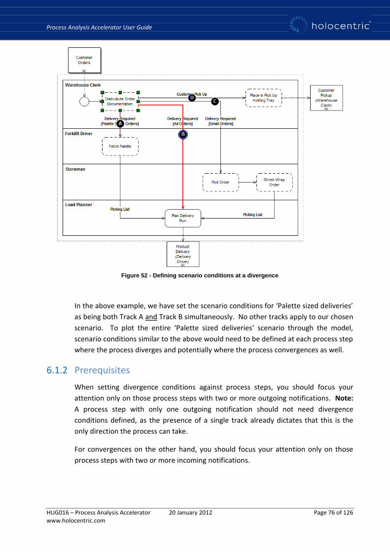
Process Analysis Accelerator User Guide
HUG016 – Process Analysis Accelerator 20 January 2012 Page 76 of 126 www.holocentric.com
Figure 52 - Defining scenario conditions at a divergence
In the above example, we have set the scenario conditions for ‘Palette sized deliveries’
as being both Track A and Track B simultaneously. No other tracks apply to our chosen
scenario. To plot the entire ‘Palette sized deliveries’ scenario through the model,
scenario conditions similar to the above would need to be defined at each process step
where the process diverges and potentially where the process convergences as well.
6.1.2 Prerequisites
When setting divergence conditions against process steps, you should focus your
attention only on those process steps with two or more outgoing notifications. Note:
A process step with only one outgoing notification should not need divergence
conditions defined, as the presence of a single track already dictates that this is the
only direction the process can take.
For convergences on the other hand, you should focus your attention only on those
process steps with two or more incoming notifications.
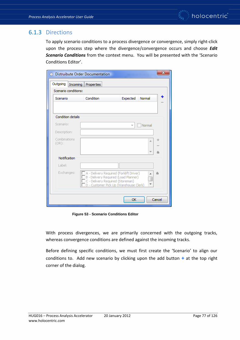
Process Analysis Accelerator User Guide
HUG016 – Process Analysis Accelerator 20 January 2012 Page 77 of 126 www.holocentric.com
6.1.3 Directions
To apply scenario conditions to a process divergence or convergence, simply right-click
upon the process step where the divergence/convergence occurs and choose Edit
Scenario Conditions from the context menu. You will be presented with the ‘Scenario
Conditions Editor’.
Figure 53 - Scenario Conditions Editor
With process divergences, we are primarily concerned with the outgoing tracks,
whereas convergence conditions are defined against the incoming tracks.
Before defining specific conditions, we must first create the ‘Scenario’ to align our
conditions to. Add new scenario by clicking upon the add button + at the top right
corner of the dialog.
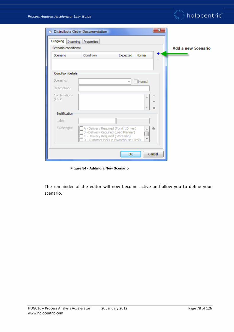
Process Analysis Accelerator User Guide
HUG016 – Process Analysis Accelerator 20 January 2012 Page 78 of 126 www.holocentric.com
Figure 54 - Adding a New Scenario
The remainder of the editor will now become active and allow you to define your
scenario.
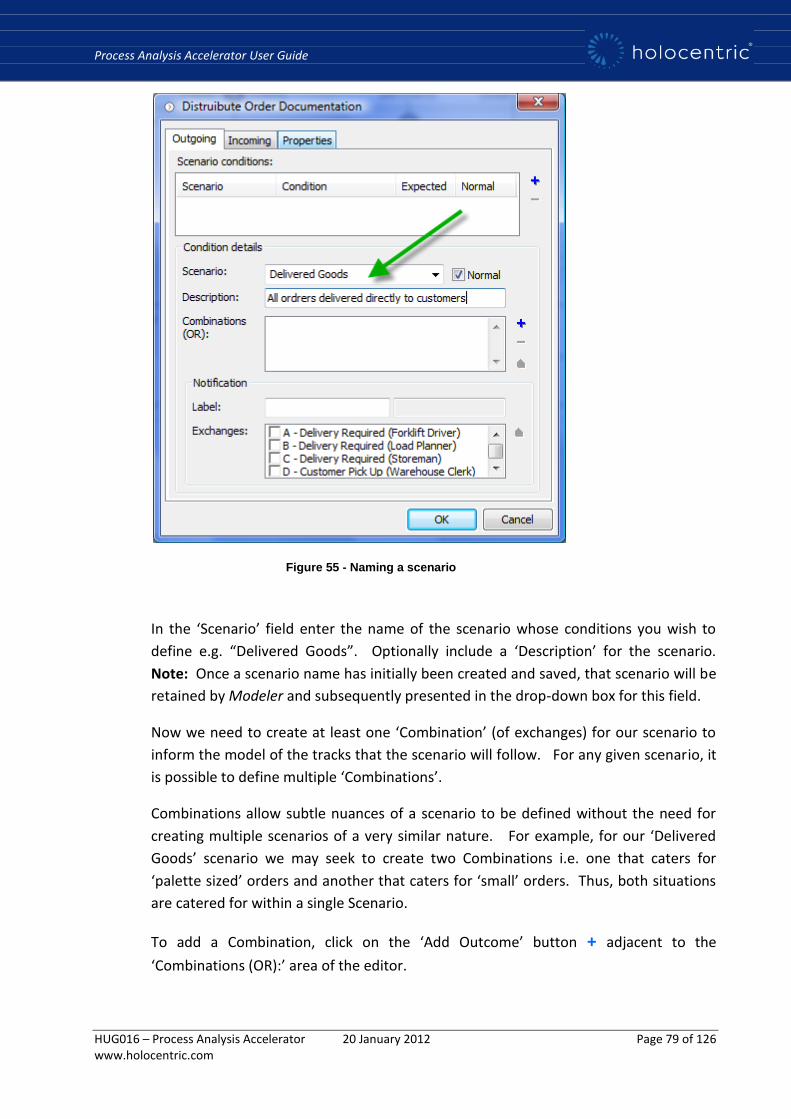
Process Analysis Accelerator User Guide
HUG016 – Process Analysis Accelerator 20 January 2012 Page 79 of 126 www.holocentric.com
Figure 55 - Naming a scenario
In the ‘Scenario’ field enter the name of the scenario whose conditions you wish to
define e.g. “Delivered Goods”. Optionally include a ‘Description’ for the scenario.
Note: Once a scenario name has initially been created and saved, that scenario will be
retained by Modeler and subsequently presented in the drop-down box for this field.
Now we need to create at least one ‘Combination’ (of exchanges) for our scenario to
inform the model of the tracks that the scenario will follow. For any given scenario, it
is possible to define multiple ‘Combinations’.
Combinations allow subtle nuances of a scenario to be defined without the need for
creating multiple scenarios of a very similar nature. For example, for our ‘Delivered
Goods’ scenario we may seek to create two Combinations i.e. one that caters for
‘palette sized’ orders and another that caters for ‘small’ orders. Thus, both situations
are catered for within a single Scenario.
To add a Combination, click on the ‘Add Outcome’ button + adjacent to the
‘Combinations (OR):’ area of the editor.

Process Analysis Accelerator User Guide
HUG016 – Process Analysis Accelerator 20 January 2012 Page 80 of 126 www.holocentric.com
Figure 56 - Adding a Combination
Enter a label for the Combination e.g. ‘Palette Sized Orders’ and choose the exchanges
that conform to this particular nuance of the ‘Delivered Goods’ scenario. Click on the
‘Add Outcome’ button + again to add a second combination for ‘Small Orders’.

Process Analysis Accelerator User Guide
HUG016 – Process Analysis Accelerator 20 January 2012 Page 81 of 126 www.holocentric.com
Figure 57 - Defining a second Combination
You should note that as you are defining the Combinations in the Scenario Conditions
Editor, the combination of exchanges is being reflected in real-time on the process
diagram in the background as shown in the following figure.
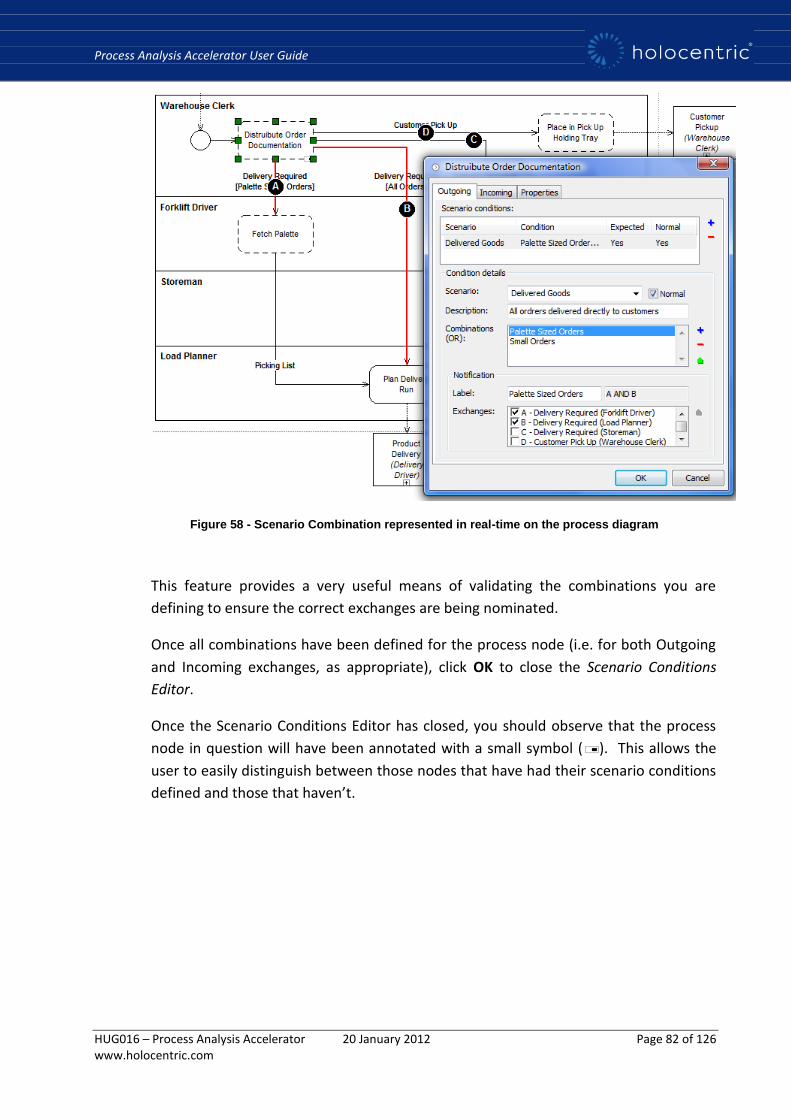
Process Analysis Accelerator User Guide
HUG016 – Process Analysis Accelerator 20 January 2012 Page 82 of 126 www.holocentric.com
Figure 58 - Scenario Combination represented in real-time on the process diagram
This feature provides a very useful means of validating the combinations you are
defining to ensure the correct exchanges are being nominated.
Once all combinations have been defined for the process node (i.e. for both Outgoing
and Incoming exchanges, as appropriate), click OK to close the Scenario Conditions
Editor.
Once the Scenario Conditions Editor has closed, you should observe that the process
node in question will have been annotated with a small symbol ( ). This allows the
user to easily distinguish between those nodes that have had their scenario conditions
defined and those that haven’t.

Process Analysis Accelerator User Guide
HUG016 – Process Analysis Accelerator 20 January 2012 Page 83 of 126 www.holocentric.com
Figure 59 - Scenario condition annotation
Process Analysis Accelerator User Guide
HUG016 – Process Analysis Accelerator 20 January 2012 Page 84 of 126 www.holocentric.com
6.1.4 Next Steps
To plot the full extent of a scenario through a process model, all divergences (and
some convergences) will need to have their scenario conditions defined. This may
entail a significant number of process steps being edited to reflect scenario conditions.
Once a scenario is fully defined, at least between the intended start and end points, it
is possible to run process simulation and constrain it entirely to that scenario. This
obviously allows for a highly specific and targeted analysis of your model.
In the next section, we will cover the analysis of a process model where that model has
been constrained by a manually defined set of scenario conditions.
6.2 Finding Paths Using Scenarios
6.2.1 Background
Performing process analysis upon a model that has scenario conditions defined is not
dissimilar to performing standard process analysis. The primary deviation from the
standard analysis is the need to establish a custom ‘Path Options’ definition which
instructs the analysis to look only for paths that conform to the scenario conditions
consigned to the model. The primary benefit of using scenario constrained process
analysis is the ability to constrain your analysis to highly specific areas of your model.
Once the custom Path Options definition is created, then the process of running the
process analysis is essentially the same. Once the simulation is executed on the
model, the result will be presented in the standard Path Analysis spreadsheet and the
paths discovered can be visualized in the model in exactly the same manner.
6.2.2 Prerequisites
In preparation for running a scenario process simulation upon your model, you should
ensure that at least the following requirements have been satisfied:-
Scenario conditions have been established against relevant process divergences
and convergences.
Start and End points have been defined to inform the simulation engine of the
analysis scope.
At least one contiguous path exists between the nominated Start and End points.
Metrics have been assigned to relevant process steps (use cases) and roles
(actors).
Volume constraints have been assigned to relevant process exchanges.
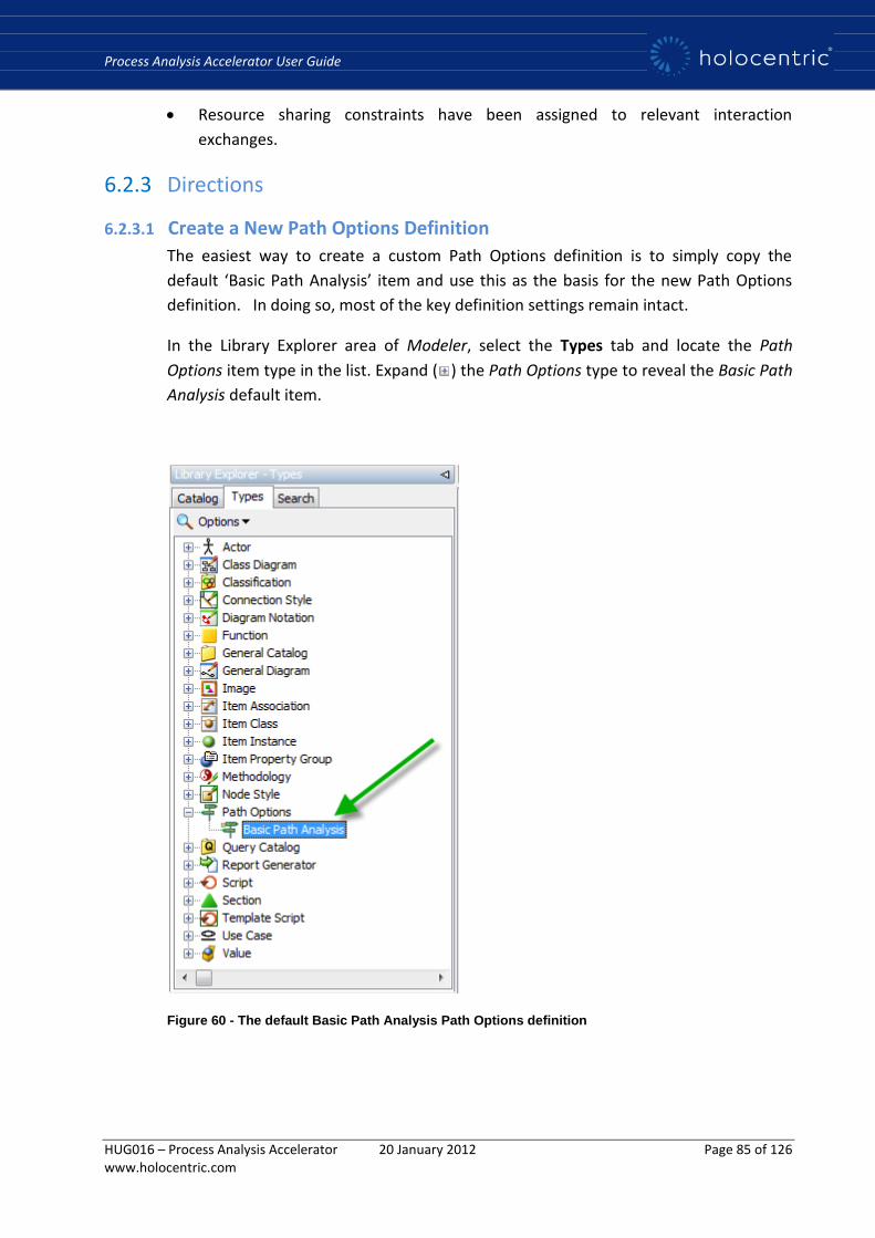
Process Analysis Accelerator User Guide
HUG016 – Process Analysis Accelerator 20 January 2012 Page 85 of 126 www.holocentric.com
Resource sharing constraints have been assigned to relevant interaction
exchanges.
6.2.3 Directions
6.2.3.1 Create a New Path Options Definition
The easiest way to create a custom Path Options definition is to simply copy the
default ‘Basic Path Analysis’ item and use this as the basis for the new Path Options
definition. In doing so, most of the key definition settings remain intact.
In the Library Explorer area of Modeler, select the Types tab and locate the Path
Options item type in the list. Expand ( ) the Path Options type to reveal the Basic Path
Analysis default item.
Figure 60 - The default Basic Path Analysis Path Options definition
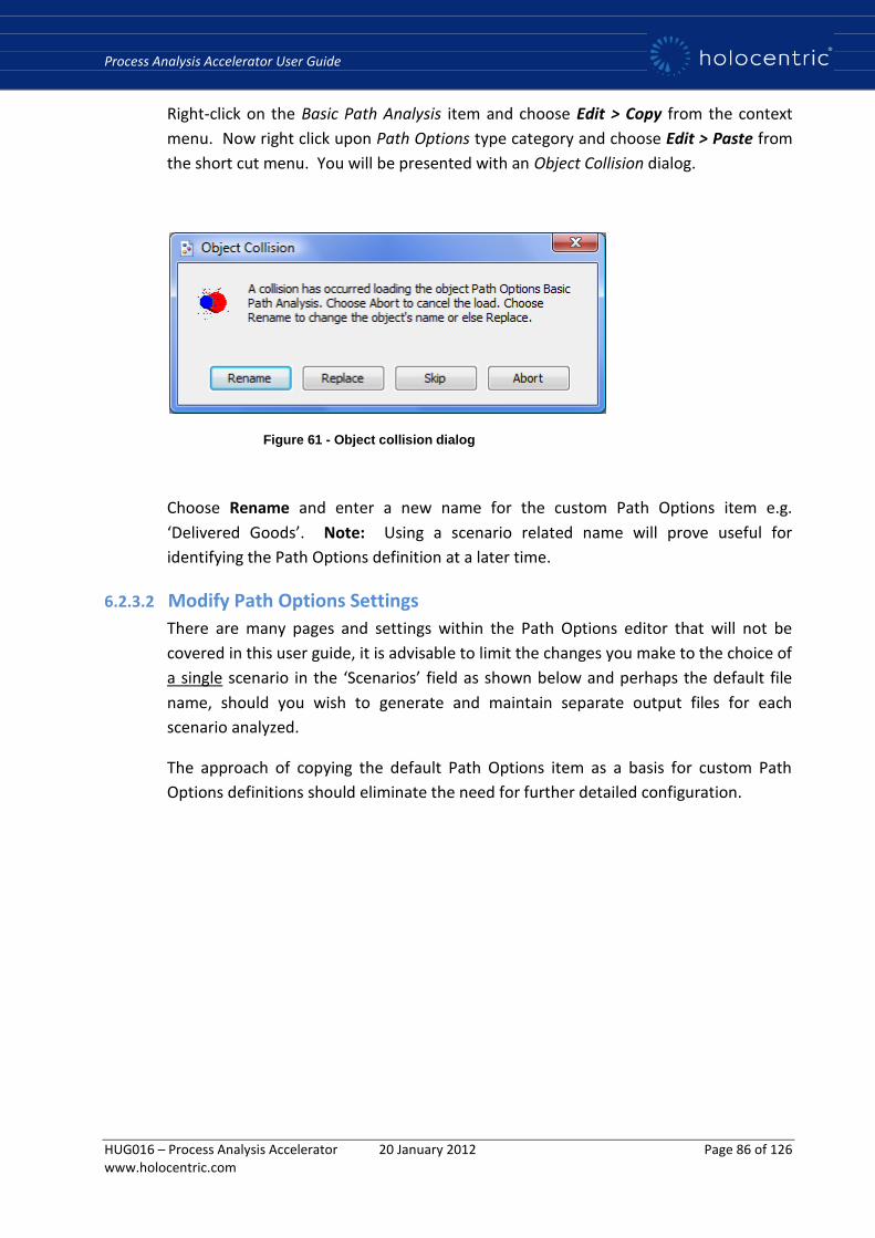
Process Analysis Accelerator User Guide
HUG016 – Process Analysis Accelerator 20 January 2012 Page 86 of 126 www.holocentric.com
Right-click on the Basic Path Analysis item and choose Edit > Copy from the context
menu. Now right click upon Path Options type category and choose Edit > Paste from
the short cut menu. You will be presented with an Object Collision dialog.
Figure 61 - Object collision dialog
Choose Rename and enter a new name for the custom Path Options item e.g.
‘Delivered Goods’. Note: Using a scenario related name will prove useful for
identifying the Path Options definition at a later time.
6.2.3.2 Modify Path Options Settings
There are many pages and settings within the Path Options editor that will not be
covered in this user guide, it is advisable to limit the changes you make to the choice of
a single scenario in the ‘Scenarios’ field as shown below and perhaps the default file
name, should you wish to generate and maintain separate output files for each
scenario analyzed.
The approach of copying the default Path Options item as a basis for custom Path
Options definitions should eliminate the need for further detailed configuration.

Process Analysis Accelerator User Guide
HUG016 – Process Analysis Accelerator 20 January 2012 Page 87 of 126 www.holocentric.com
Figure 62 - Choosing a scenario for the Path Options definition
Choose a scenario by selecting the Pick Case(s) button ( ) against the Scenario(s)
field. All unique scenarios defined within the current model (via scenario conditions)
will be returned in the resulting list. Choose the scenario that you wish to use as the
basis for this Path Options definition.
Optionally modify the File name field, should you wish to generate and maintain
separate output files for each scenario analyzed. Click Save then Close to finalise your
new Path Options definition.
6.2.3.3 Process Simulation Using a Custom Path Options Definition
With all items on your process diagram deselected (by using CTRL + D), right–click
anywhere on the diagram canvas and choose Path Analysis > Find Paths... from the
context menu. Alternatively, the simulation can also be launched by selecting Path
Analysis > Find Paths... from the Diagram menu. In either case, you will be presented
with the Find Paths dialog.
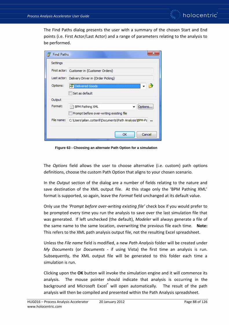
Process Analysis Accelerator User Guide
HUG016 – Process Analysis Accelerator 20 January 2012 Page 88 of 126 www.holocentric.com
The Find Paths dialog presents the user with a summary of the chosen Start and End
points (i.e. First Actor/Last Actor) and a range of parameters relating to the analysis to
be performed.
Figure 63 - Choosing an alternate Path Option for a simulation
The Options field allows the user to choose alternative (i.e. custom) path options
definitions, choose the custom Path Option that aligns to your chosen scenario.
In the Output section of the dialog are a number of fields relating to the nature and
save destination of the XML output file. At this stage only the ‘BPM Pathing XML’
format is supported, so again, leave the Format field unchanged at its default value.
Only use the ‘Prompt before over-writing existing file’ check box if you would prefer to
be prompted every time you run the analysis to save over the last simulation file that
was generated. If left unchecked (the default), Modeler will always generate a file of
the same name to the same location, overwriting the previous file each time. Note:
This refers to the XML path analysis output file, not the resulting Excel spreadsheet.
Unless the File name field is modified, a new Path Analysis folder will be created under
My Documents (or Documents - if using Vista) the first time an analysis is run.
Subsequently, the XML output file will be generated to this folder each time a
simulation is run.
Clicking upon the OK button will invoke the simulation engine and it will commence its
analysis. The mouse pointer should indicate that analysis is occurring in the
background and Microsoft Excel® will open automatically. The result of the path
analysis will then be compiled and presented within the Path Analysis spreadsheet.
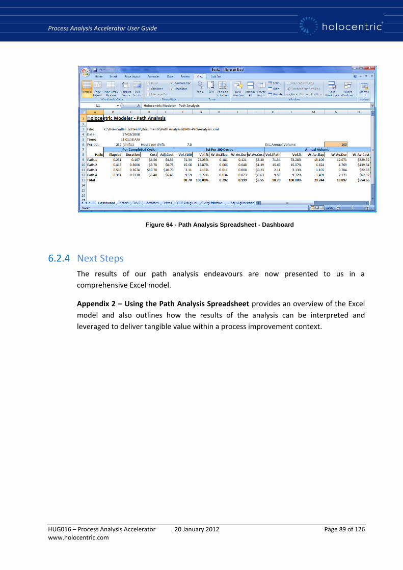
Process Analysis Accelerator User Guide
HUG016 – Process Analysis Accelerator 20 January 2012 Page 89 of 126 www.holocentric.com
Figure 64 - Path Analysis Spreadsheet - Dashboard
6.2.4 Next Steps
The results of our path analysis endeavours are now presented to us in a
comprehensive Excel model.
Appendix 2 – Using the Path Analysis Spreadsheet provides an overview of the Excel
model and also outlines how the results of the analysis can be interpreted and
leveraged to deliver tangible value within a process improvement context.
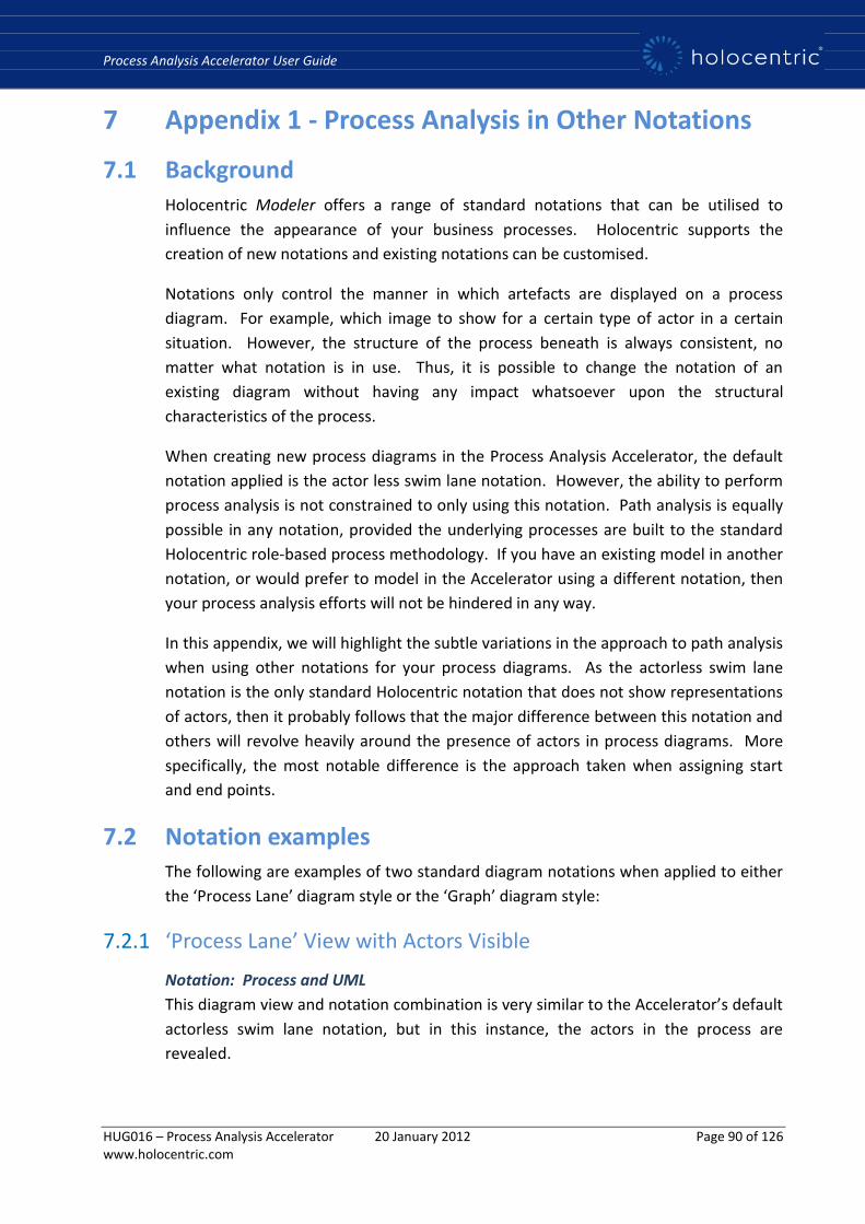
Process Analysis Accelerator User Guide
HUG016 – Process Analysis Accelerator 20 January 2012 Page 90 of 126 www.holocentric.com
7 Appendix 1 - Process Analysis in Other Notations
7.1 Background Holocentric Modeler offers a range of standard notations that can be utilised to
influence the appearance of your business processes. Holocentric supports the
creation of new notations and existing notations can be customised.
Notations only control the manner in which artefacts are displayed on a process
diagram. For example, which image to show for a certain type of actor in a certain
situation. However, the structure of the process beneath is always consistent, no
matter what notation is in use. Thus, it is possible to change the notation of an
existing diagram without having any impact whatsoever upon the structural
characteristics of the process.
When creating new process diagrams in the Process Analysis Accelerator, the default
notation applied is the actor less swim lane notation. However, the ability to perform
process analysis is not constrained to only using this notation. Path analysis is equally
possible in any notation, provided the underlying processes are built to the standard
Holocentric role-based process methodology. If you have an existing model in another
notation, or would prefer to model in the Accelerator using a different notation, then
your process analysis efforts will not be hindered in any way.
In this appendix, we will highlight the subtle variations in the approach to path analysis
when using other notations for your process diagrams. As the actorless swim lane
notation is the only standard Holocentric notation that does not show representations
of actors, then it probably follows that the major difference between this notation and
others will revolve heavily around the presence of actors in process diagrams. More
specifically, the most notable difference is the approach taken when assigning start
and end points.
7.2 Notation examples The following are examples of two standard diagram notations when applied to either
the ‘Process Lane’ diagram style or the ‘Graph’ diagram style:
7.2.1 ‘Process Lane’ View with Actors Visible
Notation: Process and UML
This diagram view and notation combination is very similar to the Accelerator’s default
actorless swim lane notation, but in this instance, the actors in the process are
revealed.
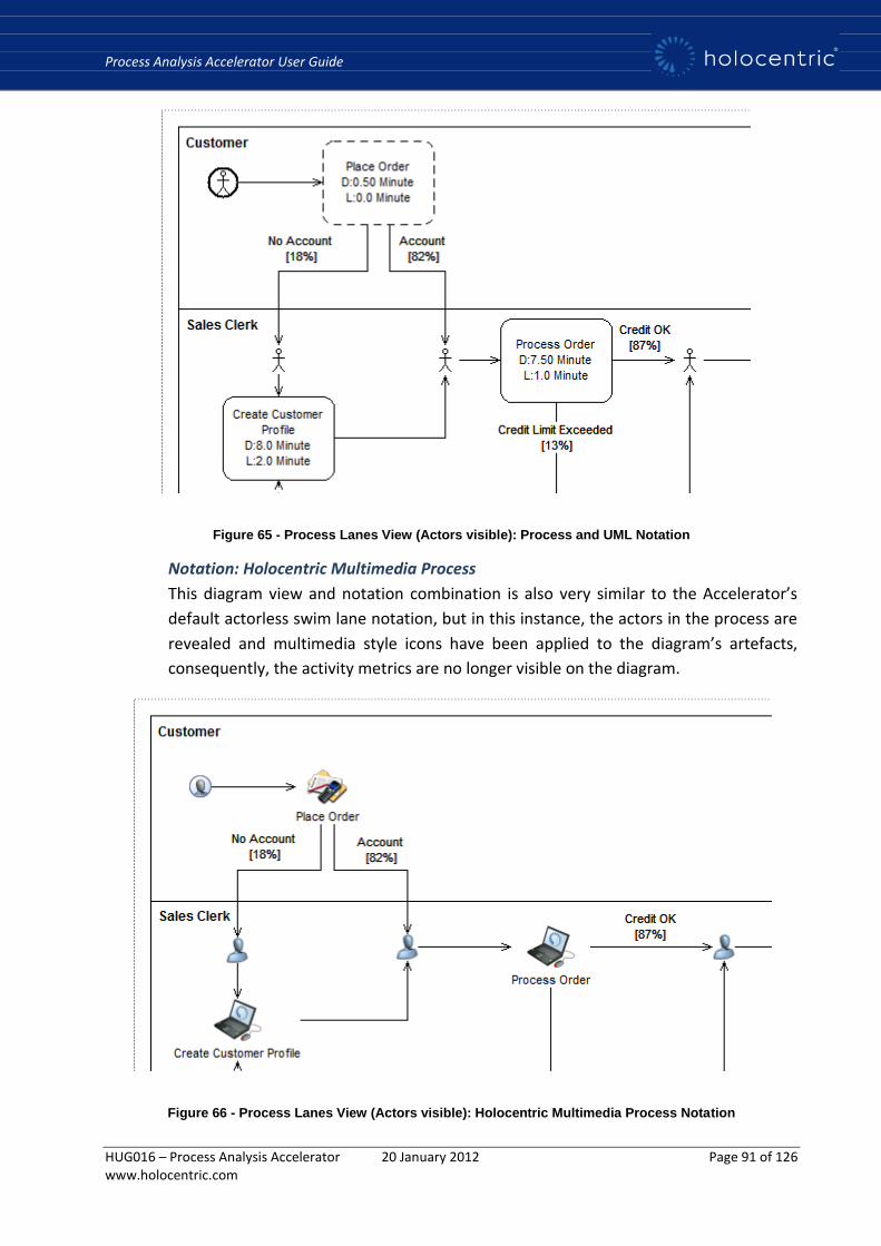
Process Analysis Accelerator User Guide
HUG016 – Process Analysis Accelerator 20 January 2012 Page 91 of 126 www.holocentric.com
Figure 65 - Process Lanes View (Actors visible): Process and UML Notation
Notation: Holocentric Multimedia Process
This diagram view and notation combination is also very similar to the Accelerator’s
default actorless swim lane notation, but in this instance, the actors in the process are
revealed and multimedia style icons have been applied to the diagram’s artefacts,
consequently, the activity metrics are no longer visible on the diagram.
Figure 66 - Process Lanes View (Actors visible): Holocentric Multimedia Process Notation

Process Analysis Accelerator User Guide
HUG016 – Process Analysis Accelerator 20 January 2012 Page 92 of 126 www.holocentric.com
7.2.2 ‘Graph’ Process View
Notation: Process and UML
The graph process view does not support the use of process lanes for actors, and
consequently all actor instances are visible on the diagram as part of the process flow.
Figure 67 - Graph process view: Process and UML Notation
Notation: Holocentric Multimedia Process
This diagram view and notation combination is identical to the previous example, but
multimedia style icons have been substituted for the black and white symbols of the
Process and UML notation.
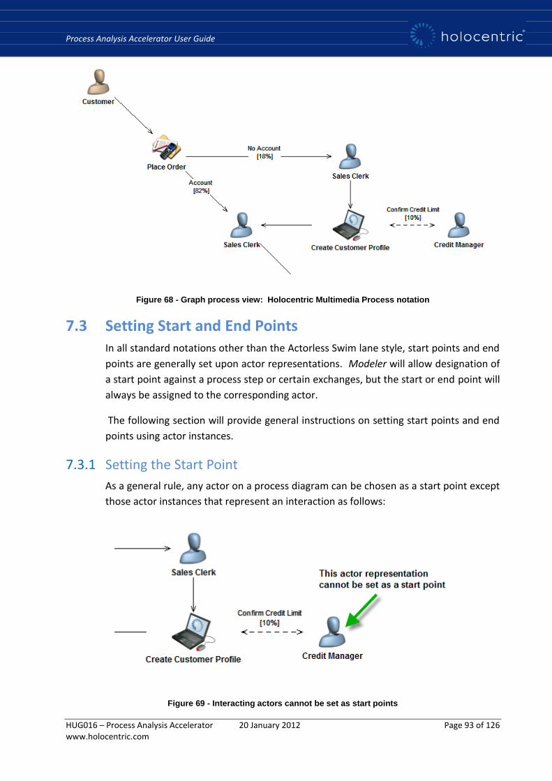
Process Analysis Accelerator User Guide
HUG016 – Process Analysis Accelerator 20 January 2012 Page 93 of 126 www.holocentric.com
Figure 68 - Graph process view: Holocentric Multimedia Process notation
7.3 Setting Start and End Points In all standard notations other than the Actorless Swim lane style, start points and end
points are generally set upon actor representations. Modeler will allow designation of
a start point against a process step or certain exchanges, but the start or end point will
always be assigned to the corresponding actor.
The following section will provide general instructions on setting start points and end
points using actor instances.
7.3.1 Setting the Start Point
As a general rule, any actor on a process diagram can be chosen as a start point except
those actor instances that represent an interaction as follows:
Figure 69 - Interacting actors cannot be set as start points
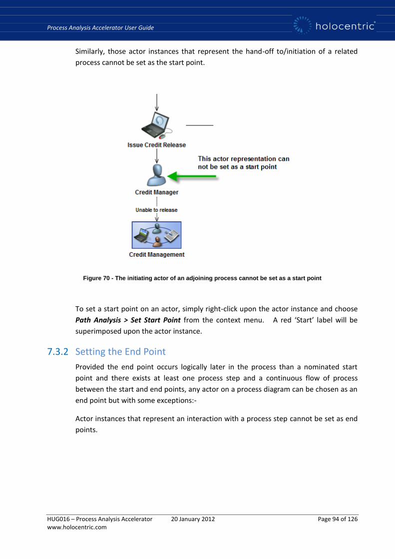
Process Analysis Accelerator User Guide
HUG016 – Process Analysis Accelerator 20 January 2012 Page 94 of 126 www.holocentric.com
Similarly, those actor instances that represent the hand-off to/initiation of a related
process cannot be set as the start point.
Figure 70 - The initiating actor of an adjoining process cannot be set as a start point
To set a start point on an actor, simply right-click upon the actor instance and choose
Path Analysis > Set Start Point from the context menu. A red ‘Start’ label will be
superimposed upon the actor instance.
7.3.2 Setting the End Point
Provided the end point occurs logically later in the process than a nominated start
point and there exists at least one process step and a continuous flow of process
between the start and end points, any actor on a process diagram can be chosen as an
end point but with some exceptions:-
Actor instances that represent an interaction with a process step cannot be set as end
points.
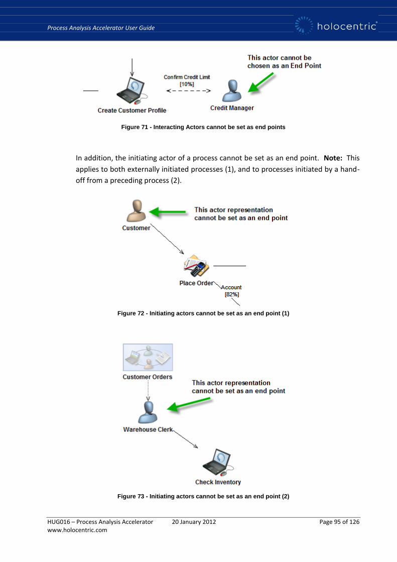
Process Analysis Accelerator User Guide
HUG016 – Process Analysis Accelerator 20 January 2012 Page 95 of 126 www.holocentric.com
Figure 71 - Interacting Actors cannot be set as end points
In addition, the initiating actor of a process cannot be set as an end point. Note: This
applies to both externally initiated processes (1), and to processes initiated by a hand-
off from a preceding process (2).
Figure 72 - Initiating actors cannot be set as an end point (1)
Figure 73 - Initiating actors cannot be set as an end point (2)
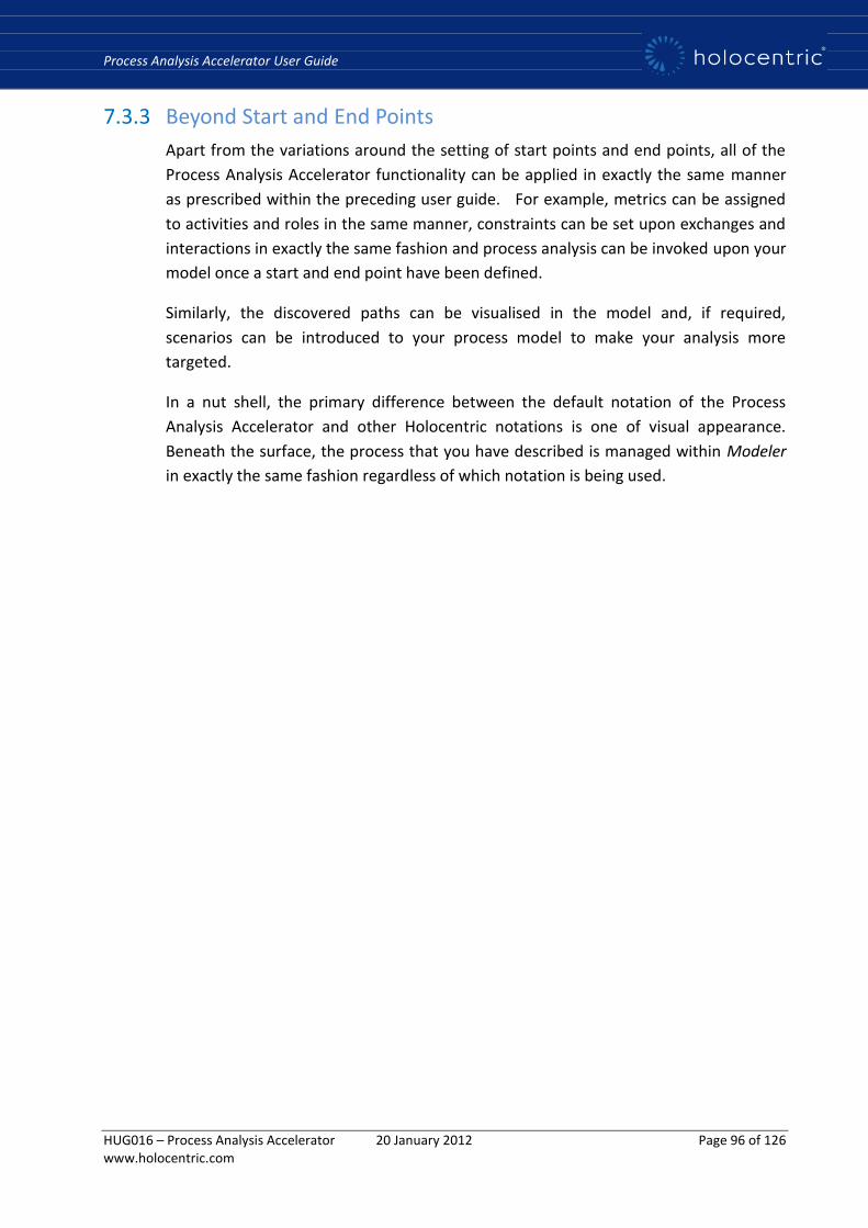
Process Analysis Accelerator User Guide
HUG016 – Process Analysis Accelerator 20 January 2012 Page 96 of 126 www.holocentric.com
7.3.3 Beyond Start and End Points
Apart from the variations around the setting of start points and end points, all of the
Process Analysis Accelerator functionality can be applied in exactly the same manner
as prescribed within the preceding user guide. For example, metrics can be assigned
to activities and roles in the same manner, constraints can be set upon exchanges and
interactions in exactly the same fashion and process analysis can be invoked upon your
model once a start and end point have been defined.
Similarly, the discovered paths can be visualised in the model and, if required,
scenarios can be introduced to your process model to make your analysis more
targeted.
In a nut shell, the primary difference between the default notation of the Process
Analysis Accelerator and other Holocentric notations is one of visual appearance.
Beneath the surface, the process that you have described is managed within Modeler
in exactly the same fashion regardless of which notation is being used.

Process Analysis Accelerator User Guide
HUG016 – Process Analysis Accelerator 20 January 2012 Page 97 of 126 www.holocentric.com
8 Appendix 2 - Using the Path Analysis Spreadsheet
8.1 Introducing the Excel Model The Excel model provided with Holocentric Modeler is aimed at supporting a basic
capability for analyzing output data from the business model, using the default options
provided in the Modeler. Beyond the scope of the spreadsheet, Modeler is capable of
performing very sophisticated Path Analysis, with highly configurable output for use in
advanced simulation engines. This capability will not, however, be covered in this user
guide.
When the result of an analysis is loaded into the spreadsheet model, the user will first
be presented with a summarised analysis result in the first worksheet, which is labelled
Dashboard.
Figure 74 - Dashboard Worksheet
Whilst the Dashboard presents a wide range of information, the information is
organized in a manner that fundamentally supports two forms of process analysis.
Specifically, the areas of the Dashboard with blue headers relate to Discrete Process
Execution Analysis, whilst the areas of the Dashboard with yellow headers relate to
Constraint and Capacity Based Analysis.
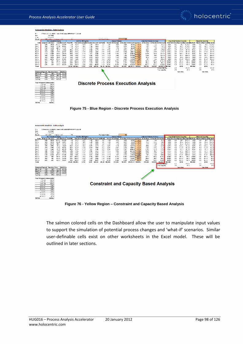
Process Analysis Accelerator User Guide
HUG016 – Process Analysis Accelerator 20 January 2012 Page 98 of 126 www.holocentric.com
Figure 75 - Blue Region - Discrete Process Execution Analysis
Figure 76 - Yellow Region – Constraint and Capacity Based Analysis
The salmon colored cells on the Dashboard allow the user to manipulate input values
to support the simulation of potential process changes and ‘what-if’ scenarios. Similar
user-definable cells exist on other worksheets in the Excel model. These will be
outlined in later sections.

Process Analysis Accelerator User Guide
HUG016 – Process Analysis Accelerator 20 January 2012 Page 99 of 126 www.holocentric.com
Figure 77 - Salmon Colored cells – User Definable Values
8.1.1 Discrete Process Execution Analysis (TDABC)
In the discrete process execution analysis view (blue headers), the Excel model can be
used to determine the contribution to the processing cost and time that is made by
each process path.
Within the discrete execution model, there is assumed to be an unlimited capacity of
labour and no pre-determined volume of activities. Instead, the model simulates the
execution of 100 complete process cycles with work distributed over the various
possible paths according to routing weightings that are defined in the process model.
It should be noted, that Path Analysis may produce Paths that contain parallel tracks,
and not just a simple linear sequence of Activities. The spreadsheet will make use of all
of the Activities included in a Path’s history, but cannot display collinear tracks in the
exact order of execution. Hence, they will appear in the spreadsheet as a single list.
The discrete execution area of the Dashboard is further divided into four sub- sections.
The first two sections (i.e. ‘Per Completed Cycle’ and ‘Est per 100 Cycles’) outline the
metrics for one cycle and 100 cycles of the process, respectively. Most values in these
sections are derived entirely from the analysis result and, hence, are unaffected by
changes made within the Excel model. The values in the Adj.Cost column, however,
are impacted by changes to role cost and/or activity overhead costs.
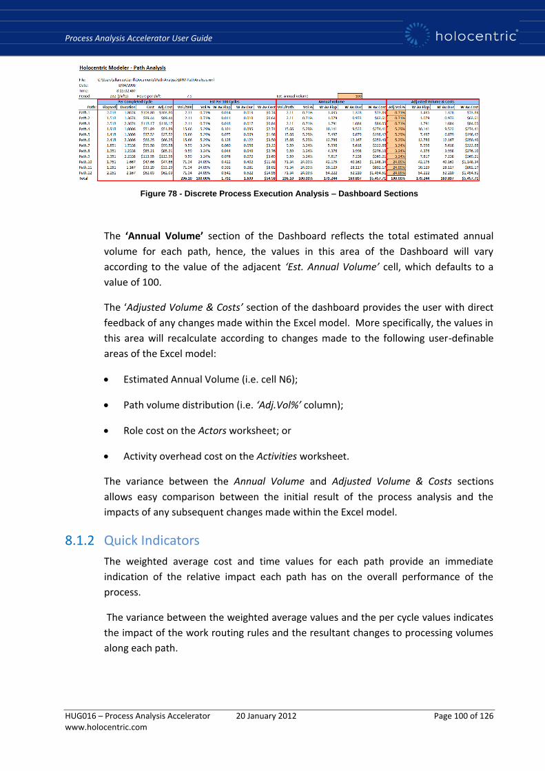
Process Analysis Accelerator User Guide
HUG016 – Process Analysis Accelerator 20 January 2012 Page 100 of 126 www.holocentric.com
Figure 78 - Discrete Process Execution Analysis – Dashboard Sections
The ‘Annual Volume’ section of the Dashboard reflects the total estimated annual
volume for each path, hence, the values in this area of the Dashboard will vary
according to the value of the adjacent ‘Est. Annual Volume’ cell, which defaults to a
value of 100.
The ‘Adjusted Volume & Costs’ section of the dashboard provides the user with direct
feedback of any changes made within the Excel model. More specifically, the values in
this area will recalculate according to changes made to the following user-definable
areas of the Excel model:
Estimated Annual Volume (i.e. cell N6);
Path volume distribution (i.e. ‘Adj.Vol%’ column);
Role cost on the Actors worksheet; or
Activity overhead cost on the Activities worksheet.
The variance between the Annual Volume and Adjusted Volume & Costs sections
allows easy comparison between the initial result of the process analysis and the
impacts of any subsequent changes made within the Excel model.
8.1.2 Quick Indicators
The weighted average cost and time values for each path provide an immediate
indication of the relative impact each path has on the overall performance of the
process.
The variance between the weighted average values and the per cycle values indicates
the impact of the work routing rules and the resultant changes to processing volumes
along each path.
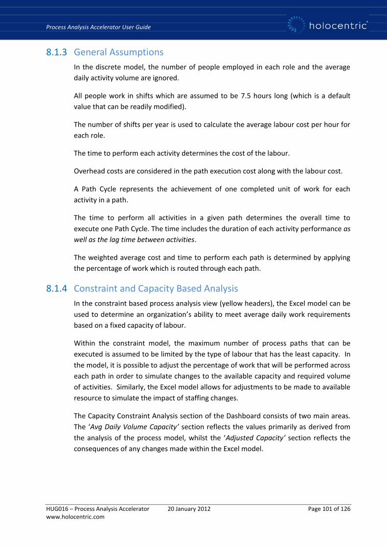
Process Analysis Accelerator User Guide
HUG016 – Process Analysis Accelerator 20 January 2012 Page 101 of 126 www.holocentric.com
8.1.3 General Assumptions
In the discrete model, the number of people employed in each role and the average
daily activity volume are ignored.
All people work in shifts which are assumed to be 7.5 hours long (which is a default
value that can be readily modified).
The number of shifts per year is used to calculate the average labour cost per hour for
each role.
The time to perform each activity determines the cost of the labour.
Overhead costs are considered in the path execution cost along with the labour cost.
A Path Cycle represents the achievement of one completed unit of work for each
activity in a path.
The time to perform all activities in a given path determines the overall time to
execute one Path Cycle. The time includes the duration of each activity performance as
well as the lag time between activities.
The weighted average cost and time to perform each path is determined by applying
the percentage of work which is routed through each path.
8.1.4 Constraint and Capacity Based Analysis
In the constraint based process analysis view (yellow headers), the Excel model can be
used to determine an organization’s ability to meet average daily work requirements
based on a fixed capacity of labour.
Within the constraint model, the maximum number of process paths that can be
executed is assumed to be limited by the type of labour that has the least capacity. In
the model, it is possible to adjust the percentage of work that will be performed across
each path in order to simulate changes to the available capacity and required volume
of activities. Similarly, the Excel model allows for adjustments to be made to available
resource to simulate the impact of staffing changes.
The Capacity Constraint Analysis section of the Dashboard consists of two main areas.
The ‘Avg Daily Volume Capacity’ section reflects the values primarily as derived from
the analysis of the process model, whilst the ‘Adjusted Capacity’ section reflects the
consequences of any changes made within the Excel model.
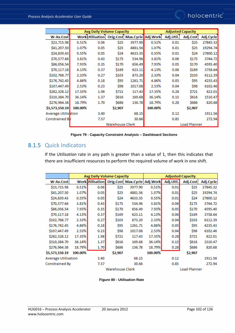
Process Analysis Accelerator User Guide
HUG016 – Process Analysis Accelerator 20 January 2012 Page 102 of 126 www.holocentric.com
Figure 79 - Capacity Constraint Analysis – Dashboard Sections
8.1.5 Quick Indicators
If the Utilisation rate in any path is greater than a value of 1, then this indicates that
there are insufficient resources to perform the required volume of work in one shift.
Figure 80 - Utilisation Rate
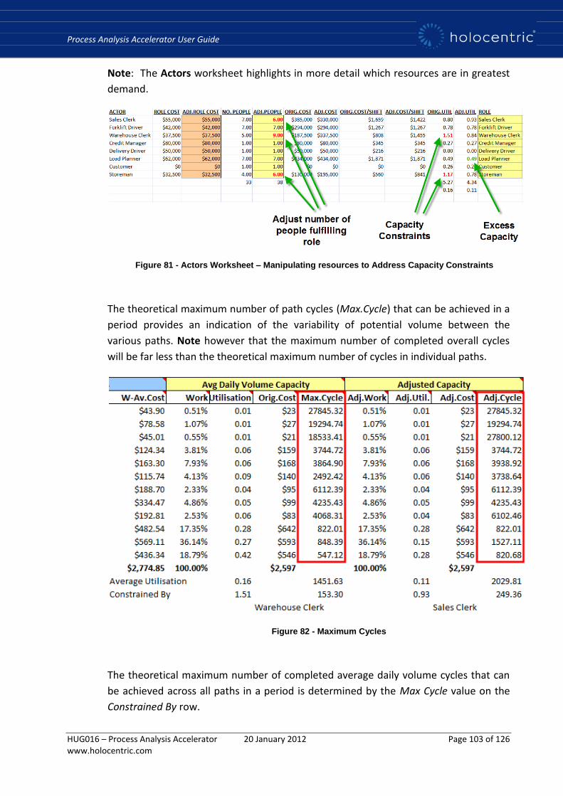
Process Analysis Accelerator User Guide
HUG016 – Process Analysis Accelerator 20 January 2012 Page 103 of 126 www.holocentric.com
Note: The Actors worksheet highlights in more detail which resources are in greatest
demand.
Figure 81 - Actors Worksheet – Manipulating resources to Address Capacity Constraints
The theoretical maximum number of path cycles (Max.Cycle) that can be achieved in a
period provides an indication of the variability of potential volume between the
various paths. Note however that the maximum number of completed overall cycles
will be far less than the theoretical maximum number of cycles in individual paths.
Figure 82 - Maximum Cycles
The theoretical maximum number of completed average daily volume cycles that can
be achieved across all paths in a period is determined by the Max Cycle value on the
Constrained By row.
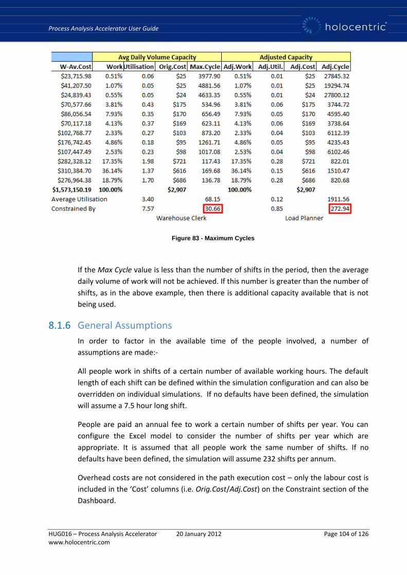
Process Analysis Accelerator User Guide
HUG016 – Process Analysis Accelerator 20 January 2012 Page 104 of 126 www.holocentric.com
Figure 83 - Maximum Cycles
If the Max Cycle value is less than the number of shifts in the period, then the average
daily volume of work will not be achieved. If this number is greater than the number of
shifts, as in the above example, then there is additional capacity available that is not
being used.
8.1.6 General Assumptions
In order to factor in the available time of the people involved, a number of
assumptions are made:-
All people work in shifts of a certain number of available working hours. The default
length of each shift can be defined within the simulation configuration and can also be
overridden on individual simulations. If no defaults have been defined, the simulation
will assume a 7.5 hour long shift.
People are paid an annual fee to work a certain number of shifts per year. You can
configure the Excel model to consider the number of shifts per year which are
appropriate. It is assumed that all people work the same number of shifts. If no
defaults have been defined, the simulation will assume 232 shifts per annum.
Overhead costs are not considered in the path execution cost – only the labour cost is
included in the ‘Cost’ columns (i.e. Orig.Cost/Adj.Cost) on the Constraint section of the
Dashboard.

Process Analysis Accelerator User Guide
HUG016 – Process Analysis Accelerator 20 January 2012 Page 105 of 126 www.holocentric.com
Figure 84 - Cost Columns
In the Actors worksheet, the model provides for adjustments to the number of people
employed in each process role and their annual fee.
Figure 85 - Actors Worksheet – Adjusting Role Cost and Number of People Playing Role
The average daily volume property of an activity describes the average volume of
activities that are required to be completed each day (i.e. in one shift).
The total shift capacity in labour hours is determined by the number of people who
play each role employed to meet the average daily volume of all work across all paths.
The ‘Work’ percentage values (i.e. Work/Adj.Work) in the Constraint section of the
Dashboard, describe the percentage of work which is channelled through each path.

Process Analysis Accelerator User Guide
HUG016 – Process Analysis Accelerator 20 January 2012 Page 106 of 126 www.holocentric.com
The percentage of work is used to calculate the share of the average daily activity
volume that is required to be performed in each path.
Figure 86 - Work Columns
A complete Shift Cycle is achieved when the average daily volume of all activities which
are performed across all paths is achieved.
A Path Cycle represents the achievement of the daily volume of work in a path, given
the activities within that path and the work % allocated to that path.
The maximum Shift Cycles that can be achieved will be determined by the capacity of
the role that has the greatest utilisation.
8.1.7 Exploring the Excel Model in Detail
The following section provides a general summary of all worksheets within the Excel
model and, where relevant, highlights the key elements of these worksheets.
Most worksheets in the Excel model are entirely informational in nature. However,
the Dashboard, Actors and Activities worksheets all support user definable cells which
can be manipulated to influence the analysis. All editable cells in the Excel model are
colored either yellow or salmon.
Note: Changing yellow colored cells will directly impact the capacity constraint
analysis view, whereas changing salmon colored cells will impact both the capacity
constraint view and the discrete process execution view.
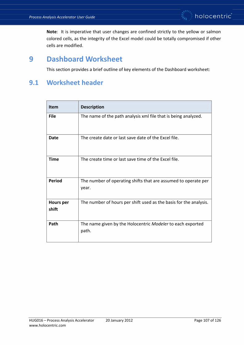
Process Analysis Accelerator User Guide
HUG016 – Process Analysis Accelerator 20 January 2012 Page 107 of 126 www.holocentric.com
Note: It is imperative that user changes are confined strictly to the yellow or salmon
colored cells, as the integrity of the Excel model could be totally compromised if other
cells are modified.
9 Dashboard Worksheet This section provides a brief outline of key elements of the Dashboard worksheet:
9.1 Worksheet header
Item Description
File The name of the path analysis xml file that is being analyzed.
Date The create date or last save date of the Excel file.
Time The create time or last save time of the Excel file.
Period The number of operating shifts that are assumed to operate per
year.
Hours per
shift
The number of hours per shift used as the basis for the analysis.
Path
The name given by the Holocentric Modeler to each exported
path.
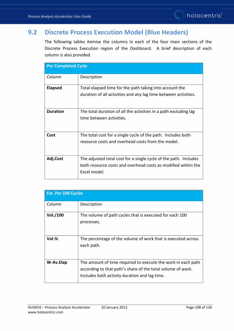
Process Analysis Accelerator User Guide
HUG016 – Process Analysis Accelerator 20 January 2012 Page 108 of 126 www.holocentric.com
9.2 Discrete Process Execution Model (Blue Headers) The following tables itemise the columns in each of the four main sections of the
Discrete Process Execution region of the Dashboard. A brief description of each
column is also provided.
Per Completed Cycle
Column Description
Elapsed Total elapsed time for the path taking into account the
duration of all activities and any lag time between activities.
Duration The total duration of all the activities in a path excluding lag
time between activities.
Cost The total cost for a single cycle of the path. Includes both
resource costs and overhead costs from the model.
Adj.Cost The adjusted total cost for a single cycle of the path. Includes
both resource costs and overhead costs as modified within the
Excel model.
Est. Per 100 Cycles
Column Description
Vol./100 The volume of path cycles that is executed for each 100
processes.
Vol.% The percentage of the volume of work that is executed across
each path.
W-Av.Elap The amount of time required to execute the work in each path
according to that path’s share of the total volume of work.
Includes both activity duration and lag time.
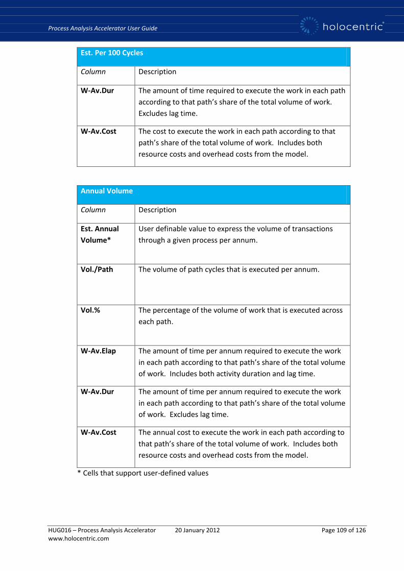
Process Analysis Accelerator User Guide
HUG016 – Process Analysis Accelerator 20 January 2012 Page 109 of 126 www.holocentric.com
Est. Per 100 Cycles
Column Description
W-Av.Dur The amount of time required to execute the work in each path
according to that path’s share of the total volume of work.
Excludes lag time.
W-Av.Cost The cost to execute the work in each path according to that
path’s share of the total volume of work. Includes both
resource costs and overhead costs from the model.
Annual Volume
Column Description
Est. Annual
Volume*
User definable value to express the volume of transactions
through a given process per annum.
Vol./Path The volume of path cycles that is executed per annum.
Vol.% The percentage of the volume of work that is executed across
each path.
W-Av.Elap The amount of time per annum required to execute the work
in each path according to that path’s share of the total volume
of work. Includes both activity duration and lag time.
W-Av.Dur The amount of time per annum required to execute the work
in each path according to that path’s share of the total volume
of work. Excludes lag time.
W-Av.Cost The annual cost to execute the work in each path according to
that path’s share of the total volume of work. Includes both
resource costs and overhead costs from the model.
* Cells that support user-defined values
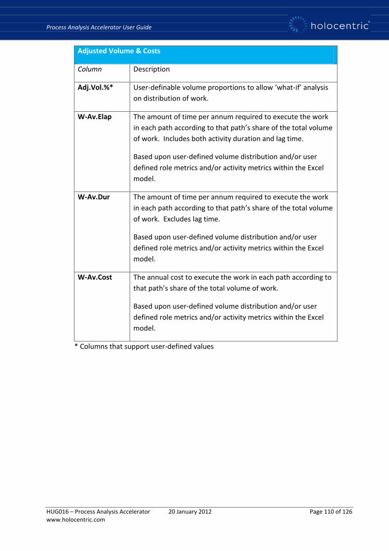
Process Analysis Accelerator User Guide
HUG016 – Process Analysis Accelerator 20 January 2012 Page 110 of 126 www.holocentric.com
Adjusted Volume & Costs
Column Description
Adj.Vol.%* User-definable volume proportions to allow ‘what-if’ analysis
on distribution of work.
W-Av.Elap The amount of time per annum required to execute the work
in each path according to that path’s share of the total volume
of work. Includes both activity duration and lag time.
Based upon user-defined volume distribution and/or user
defined role metrics and/or activity metrics within the Excel
model.
W-Av.Dur The amount of time per annum required to execute the work
in each path according to that path’s share of the total volume
of work. Excludes lag time.
Based upon user-defined volume distribution and/or user
defined role metrics and/or activity metrics within the Excel
model.
W-Av.Cost The annual cost to execute the work in each path according to
that path’s share of the total volume of work.
Based upon user-defined volume distribution and/or user
defined role metrics and/or activity metrics within the Excel
model.
* Columns that support user-defined values
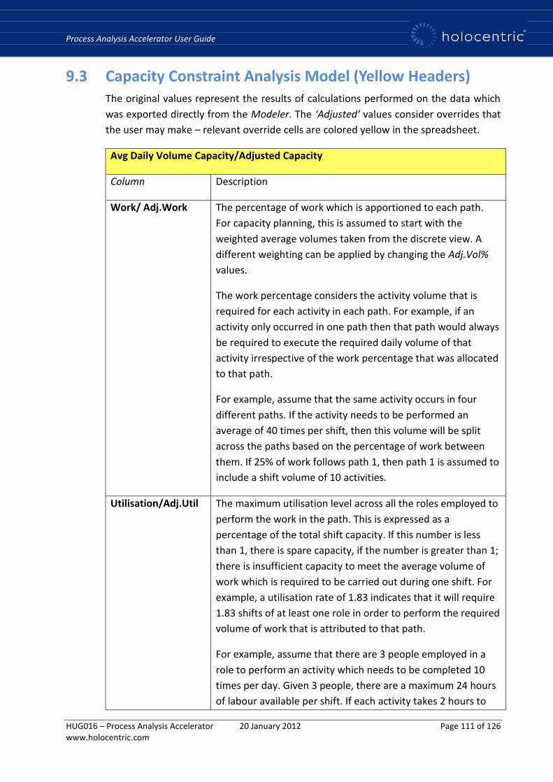
Process Analysis Accelerator User Guide
HUG016 – Process Analysis Accelerator 20 January 2012 Page 111 of 126 www.holocentric.com
9.3 Capacity Constraint Analysis Model (Yellow Headers) The original values represent the results of calculations performed on the data which
was exported directly from the Modeler. The ‘Adjusted’ values consider overrides that
the user may make – relevant override cells are colored yellow in the spreadsheet.
Avg Daily Volume Capacity/Adjusted Capacity
Column Description
Work/ Adj.Work The percentage of work which is apportioned to each path.
For capacity planning, this is assumed to start with the
weighted average volumes taken from the discrete view. A
different weighting can be applied by changing the Adj.Vol%
values.
The work percentage considers the activity volume that is
required for each activity in each path. For example, if an
activity only occurred in one path then that path would always
be required to execute the required daily volume of that
activity irrespective of the work percentage that was allocated
to that path.
For example, assume that the same activity occurs in four
different paths. If the activity needs to be performed an
average of 40 times per shift, then this volume will be split
across the paths based on the percentage of work between
them. If 25% of work follows path 1, then path 1 is assumed to
include a shift volume of 10 activities.
Utilisation/Adj.Util The maximum utilisation level across all the roles employed to
perform the work in the path. This is expressed as a
percentage of the total shift capacity. If this number is less
than 1, there is spare capacity, if the number is greater than 1;
there is insufficient capacity to meet the average volume of
work which is required to be carried out during one shift. For
example, a utilisation rate of 1.83 indicates that it will require
1.83 shifts of at least one role in order to perform the required
volume of work that is attributed to that path.
For example, assume that there are 3 people employed in a
role to perform an activity which needs to be completed 10
times per day. Given 3 people, there are a maximum 24 hours
of labour available per shift. If each activity takes 2 hours to

Process Analysis Accelerator User Guide
HUG016 – Process Analysis Accelerator 20 January 2012 Page 112 of 126 www.holocentric.com
Avg Daily Volume Capacity/Adjusted Capacity
Column Description
perform, it will require 20 hours of labour to complete the 10
activities per shift. In terms of the shifts required, it would
require 0.83 shifts of the role workforce to complete the
required work.
The utilisation level of each role is described in more detail on
the Actors worksheet.
The Average Utilisation indicates the average number of shifts
that would be required to be performed by each employed
person to meet the average daily volume of work.
The Constrained By value indicates the maximum utilisation
level of any role across all paths. This value represents the
theoretical maximum number of cycles that could be
performed in a year.
The name of the role with the maximum utilisation is
displayed next to the utilisation value. If more than one role
has the same maximum utilisation value, the first role found
to have that value is displayed.
Orig.Cost/Adj.Cost The labour cost of performing the work that is required in
each shift.
The cost of each path cycle is calculated as the cost of labour
to perform the average daily volume of work in one shift.
Max.Cycle/Adj.Cycle The theoretical number of path cycles that could be
completed in a year given the path specific maximum
utilisation of staff and the weighted path volume of work.
The number of path cycles that can be processed in a year is
calculated as the shifts per year / Shift Utilisation.
9.4 Actors Worksheet The Actor worksheet contains all of the metrics associated with the roles in the
process. Whilst most of the values in this worksheet are sourced directly from the

Process Analysis Accelerator User Guide
HUG016 – Process Analysis Accelerator 20 January 2012 Page 113 of 126 www.holocentric.com
process model, the yellow and salmon colored cells can be manipulated to influence
the analysis.
Note: Changing the yellow colored cells will affect only the Adjusted Capacity area of
the Dashboard (i.e. the Capacity Constraint View), whereas changing the salmon
colored cells will affect both the Capacity Constraint view and the Discrete Process
Execution view.
Column Description
Actor
The name of the role specified in the Model.
Role Cost
The average annual cost which is associated with each role in
the Model.
Adj. Role
Cost*
An adjustable annual cost value for each role.
No. People
The number of people who fulfil the role as defined in the
model.
Adj. People*
An adjustable number of people fulfilling each role.
Orig. Cost
The total cost of employing all the people in the role.
Adj. Cost
The total cost of the adjusted number of people employed.
Adj. Cost/Shift
The total adjusted cost of employing all the people in the role
for one shift.
Orig Util.
(Original
Utilisation)
The total labour utilisation of that role per shift across all
paths.
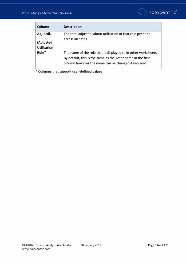
Process Analysis Accelerator User Guide
HUG016 – Process Analysis Accelerator 20 January 2012 Page 114 of 126 www.holocentric.com
Column Description
Adj. Util.
(Adjusted
Utilisation)
The total adjusted labour utilisation of that role per shift
across all paths.
Role*
The name of the role that is displayed to in other worksheets.
By default, this is the same as the Actor name in the first
column however the name can be changed if required.
* Columns that support user-defined values
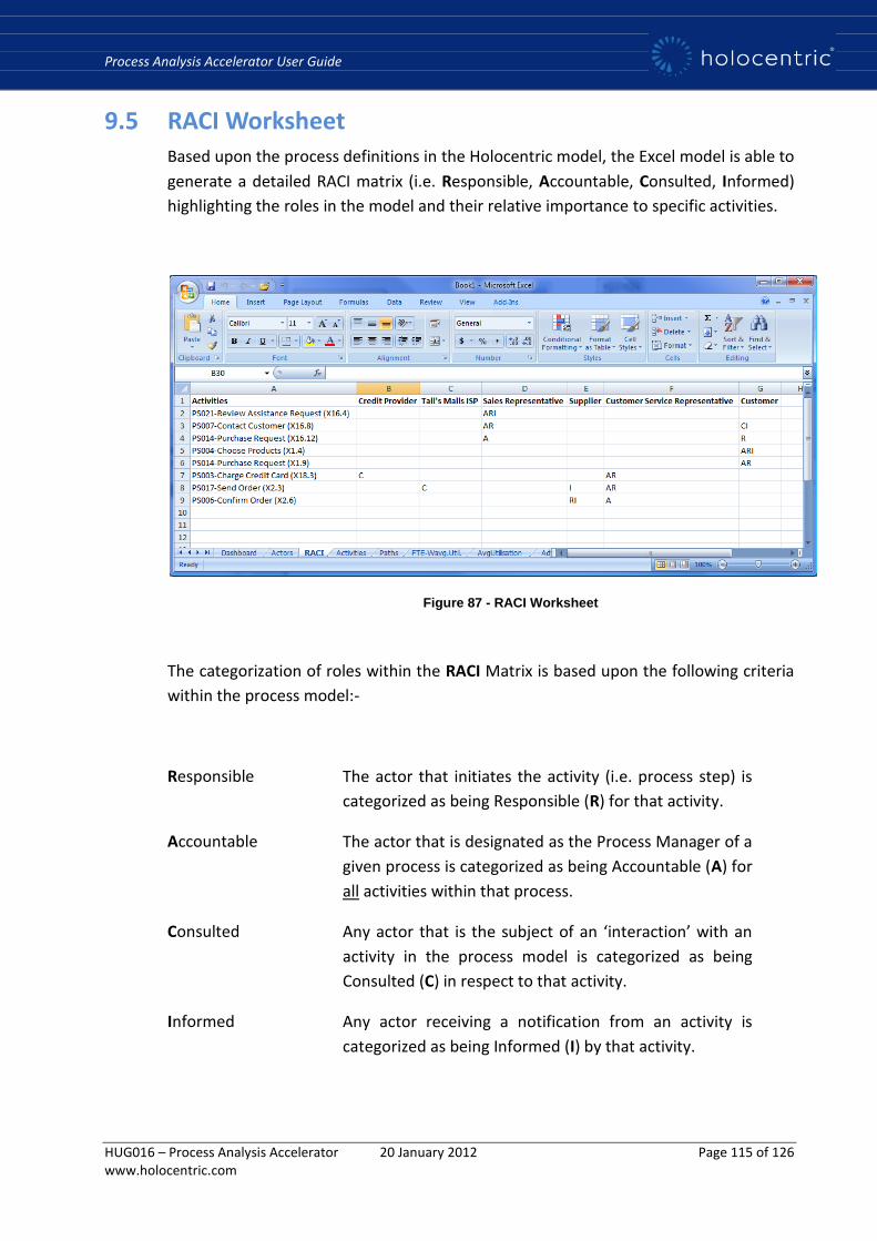
Process Analysis Accelerator User Guide
HUG016 – Process Analysis Accelerator 20 January 2012 Page 115 of 126 www.holocentric.com
9.5 RACI Worksheet Based upon the process definitions in the Holocentric model, the Excel model is able to
generate a detailed RACI matrix (i.e. Responsible, Accountable, Consulted, Informed)
highlighting the roles in the model and their relative importance to specific activities.
Figure 87 - RACI Worksheet
The categorization of roles within the RACI Matrix is based upon the following criteria
within the process model:-
Responsible The actor that initiates the activity (i.e. process step) is
categorized as being Responsible (R) for that activity.
Accountable The actor that is designated as the Process Manager of a
given process is categorized as being Accountable (A) for
all activities within that process.
Consulted Any actor that is the subject of an ‘interaction’ with an
activity in the process model is categorized as being
Consulted (C) in respect to that activity.
Informed Any actor receiving a notification from an activity is
categorized as being Informed (I) by that activity.
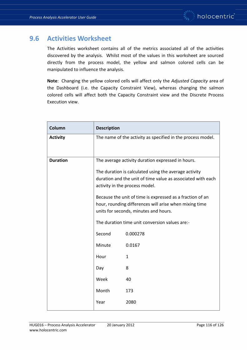
Process Analysis Accelerator User Guide
HUG016 – Process Analysis Accelerator 20 January 2012 Page 116 of 126 www.holocentric.com
9.6 Activities Worksheet The Activities worksheet contains all of the metrics associated all of the activities
discovered by the analysis. Whilst most of the values in this worksheet are sourced
directly from the process model, the yellow and salmon colored cells can be
manipulated to influence the analysis.
Note: Changing the yellow colored cells will affect only the Adjusted Capacity area of
the Dashboard (i.e. the Capacity Constraint View), whereas changing the salmon
colored cells will affect both the Capacity Constraint view and the Discrete Process
Execution view.
Column Description
Activity
The name of the activity as specified in the process model.
Duration
The average activity duration expressed in hours.
The duration is calculated using the average activity
duration and the unit of time value as associated with each
activity in the process model.
Because the unit of time is expressed as a fraction of an
hour, rounding differences will arise when mixing time
units for seconds, minutes and hours.
The duration time unit conversion values are:-
Second 0.000278
Minute 0.0167
Hour 1
Day 8
Week 40
Month 173
Year 2080
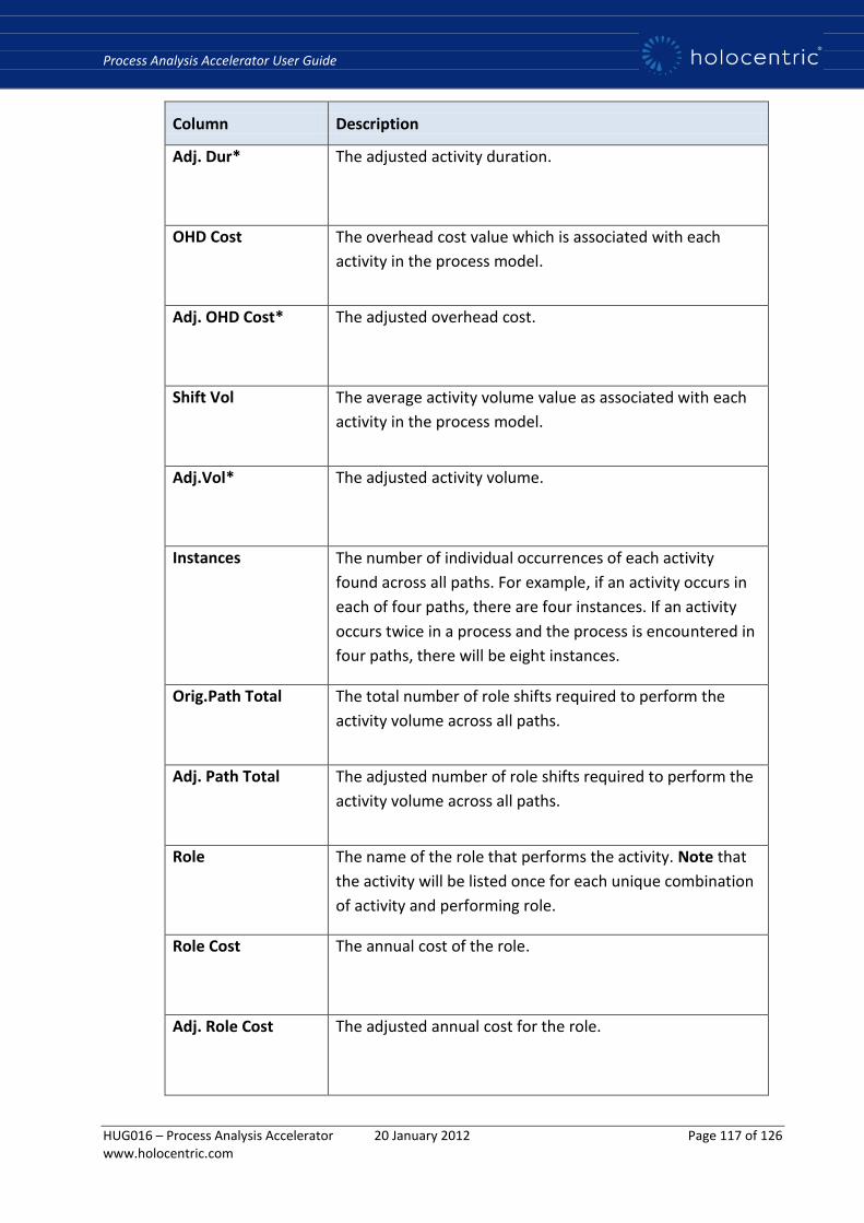
Process Analysis Accelerator User Guide
HUG016 – Process Analysis Accelerator 20 January 2012 Page 117 of 126 www.holocentric.com
Column Description
Adj. Dur*
The adjusted activity duration.
OHD Cost
The overhead cost value which is associated with each
activity in the process model.
Adj. OHD Cost*
The adjusted overhead cost.
Shift Vol
The average activity volume value as associated with each
activity in the process model.
Adj.Vol*
The adjusted activity volume.
Instances
The number of individual occurrences of each activity
found across all paths. For example, if an activity occurs in
each of four paths, there are four instances. If an activity
occurs twice in a process and the process is encountered in
four paths, there will be eight instances.
Orig.Path Total
The total number of role shifts required to perform the
activity volume across all paths.
Adj. Path Total
The adjusted number of role shifts required to perform the
activity volume across all paths.
Role
The name of the role that performs the activity. Note that
the activity will be listed once for each unique combination
of activity and performing role.
Role Cost
The annual cost of the role.
Adj. Role Cost
The adjusted annual cost for the role.
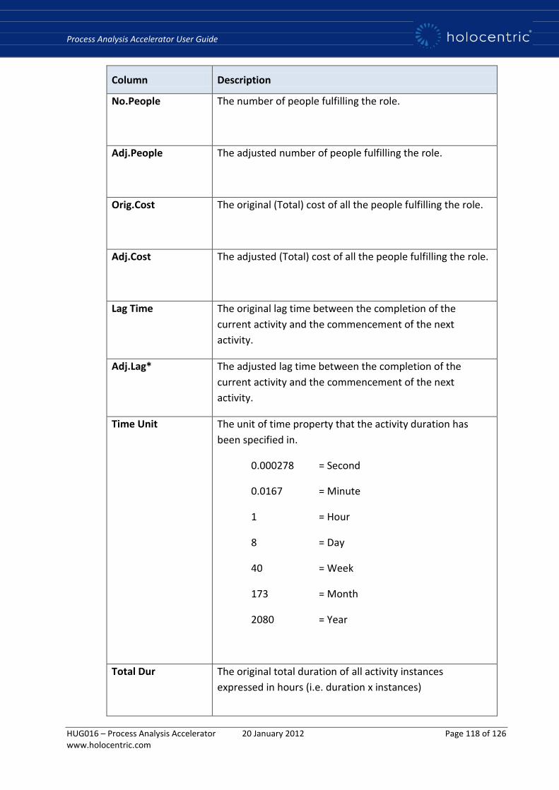
Process Analysis Accelerator User Guide
HUG016 – Process Analysis Accelerator 20 January 2012 Page 118 of 126 www.holocentric.com
Column Description
No.People
The number of people fulfilling the role.
Adj.People
The adjusted number of people fulfilling the role.
Orig.Cost
The original (Total) cost of all the people fulfilling the role.
Adj.Cost
The adjusted (Total) cost of all the people fulfilling the role.
Lag Time
The original lag time between the completion of the
current activity and the commencement of the next
activity.
Adj.Lag*
The adjusted lag time between the completion of the
current activity and the commencement of the next
activity.
Time Unit
The unit of time property that the activity duration has
been specified in.
0.000278 = Second
0.0167 = Minute
1 = Hour
8 = Day
40 = Week
173 = Month
2080 = Year
Total Dur
The original total duration of all activity instances
expressed in hours (i.e. duration x instances)

Process Analysis Accelerator User Guide
HUG016 – Process Analysis Accelerator 20 January 2012 Page 119 of 126 www.holocentric.com
Column Description
Adj.Tot.Dur
The adjusted total duration of all activity instances
expressed in hours (i.e. adj.dur x instances)
Orig Work
The original proportion of total workload that includes the
activity.
Adj.Work
The adjusted proportion of total workload that includes the
activity.
ID
A unique activity identifier.
Activity Type
The nature of the activity as designated in the process
model e.g. Rework, Duplication.
avgActivityDuration The raw duration value (prior to conversion to hours) as
sourced from the process model.
avgCostperActivity The raw activity cost value as sourced from the process
model.
avgDailyVolume The raw daily volume value as sourced from the process
model.
avgActivityLag The raw duration value (prior to conversion to hours) as
sourced from the process model.
activityAnalysisType The nature of the activity as designated in the process
model e.g. Rework, Duplication.
activityCoreYn The ‘core value activity’ value as sourced from the process
model (i.e. core value activity = Yes)
avgActivityTimeUnit The raw unit of time property that the activity duration has
been specified in.
0.000278 = Second
0.0167 = Minute
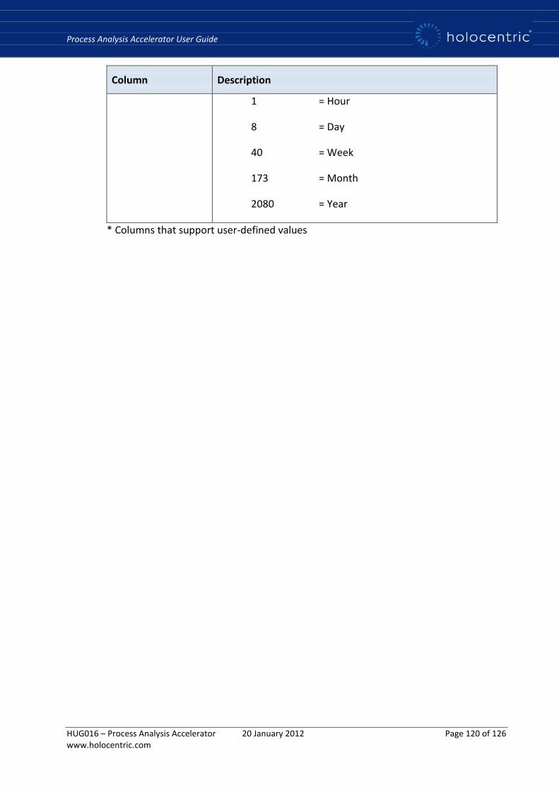
Process Analysis Accelerator User Guide
HUG016 – Process Analysis Accelerator 20 January 2012 Page 120 of 126 www.holocentric.com
Column Description
1 = Hour
8 = Day
40 = Week
173 = Month
2080 = Year
* Columns that support user-defined values
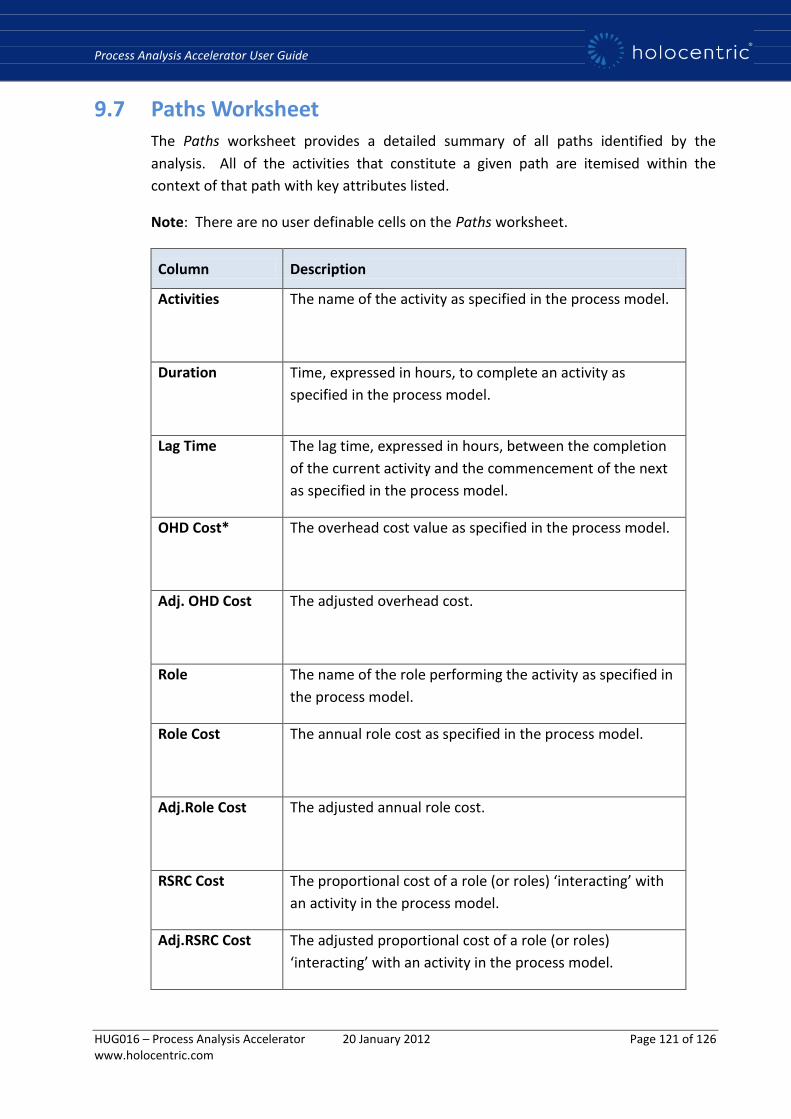
Process Analysis Accelerator User Guide
HUG016 – Process Analysis Accelerator 20 January 2012 Page 121 of 126 www.holocentric.com
9.7 Paths Worksheet The Paths worksheet provides a detailed summary of all paths identified by the
analysis. All of the activities that constitute a given path are itemised within the
context of that path with key attributes listed.
Note: There are no user definable cells on the Paths worksheet.
Column Description
Activities
The name of the activity as specified in the process model.
Duration
Time, expressed in hours, to complete an activity as
specified in the process model.
Lag Time
The lag time, expressed in hours, between the completion
of the current activity and the commencement of the next
as specified in the process model.
OHD Cost*
The overhead cost value as specified in the process model.
Adj. OHD Cost
The adjusted overhead cost.
Role The name of the role performing the activity as specified in
the process model.
Role Cost
The annual role cost as specified in the process model.
Adj.Role Cost
The adjusted annual role cost.
RSRC Cost The proportional cost of a role (or roles) ‘interacting’ with
an activity in the process model.
Adj.RSRC Cost The adjusted proportional cost of a role (or roles)
‘interacting’ with an activity in the process model.
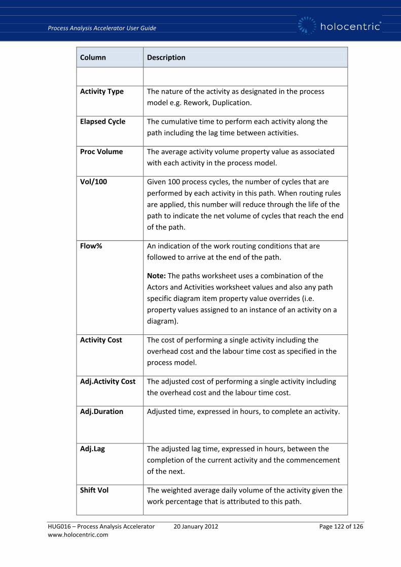
Process Analysis Accelerator User Guide
HUG016 – Process Analysis Accelerator 20 January 2012 Page 122 of 126 www.holocentric.com
Column Description
Activity Type The nature of the activity as designated in the process
model e.g. Rework, Duplication.
Elapsed Cycle The cumulative time to perform each activity along the
path including the lag time between activities.
Proc Volume The average activity volume property value as associated
with each activity in the process model.
Vol/100 Given 100 process cycles, the number of cycles that are
performed by each activity in this path. When routing rules
are applied, this number will reduce through the life of the
path to indicate the net volume of cycles that reach the end
of the path.
Flow% An indication of the work routing conditions that are
followed to arrive at the end of the path.
Note: The paths worksheet uses a combination of the
Actors and Activities worksheet values and also any path
specific diagram item property value overrides (i.e.
property values assigned to an instance of an activity on a
diagram).
Activity Cost The cost of performing a single activity including the
overhead cost and the labour time cost as specified in the
process model.
Adj.Activity Cost The adjusted cost of performing a single activity including
the overhead cost and the labour time cost.
Adj.Duration Adjusted time, expressed in hours, to complete an activity.
Adj.Lag The adjusted lag time, expressed in hours, between the
completion of the current activity and the commencement
of the next.
Shift Vol The weighted average daily volume of the activity given the
work percentage that is attributed to this path.
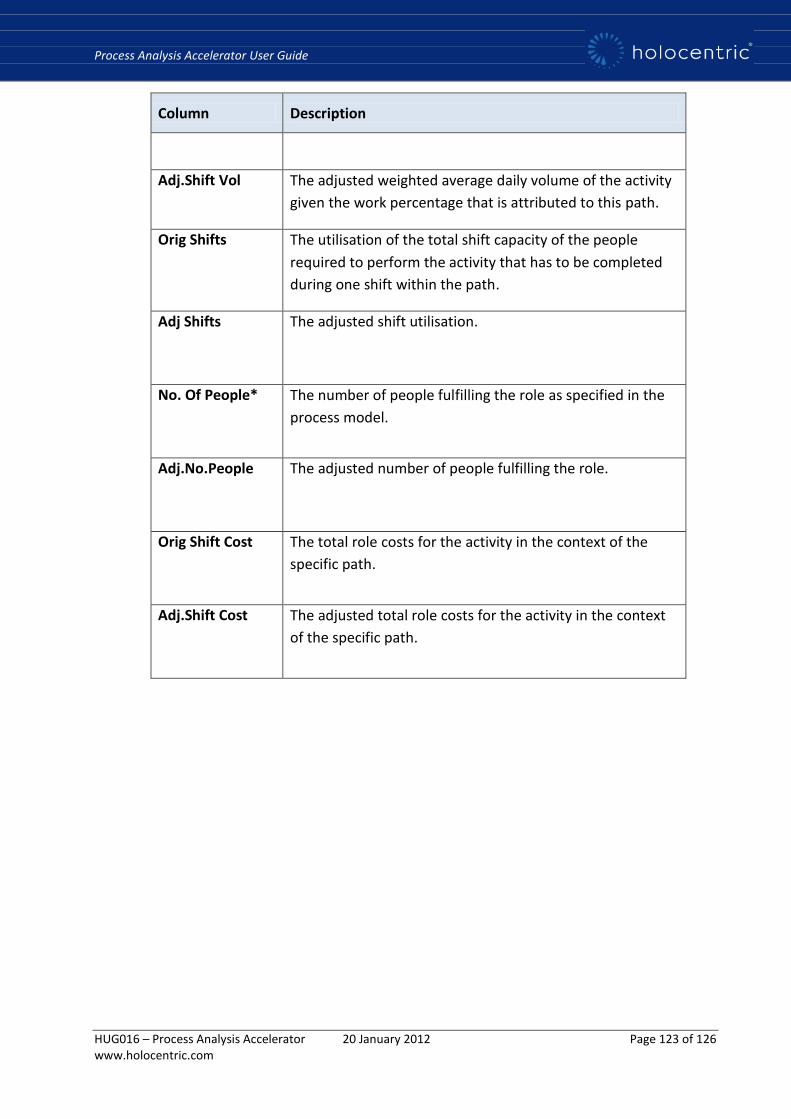
Process Analysis Accelerator User Guide
HUG016 – Process Analysis Accelerator 20 January 2012 Page 123 of 126 www.holocentric.com
Column Description
Adj.Shift Vol The adjusted weighted average daily volume of the activity
given the work percentage that is attributed to this path.
Orig Shifts
The utilisation of the total shift capacity of the people
required to perform the activity that has to be completed
during one shift within the path.
Adj Shifts
The adjusted shift utilisation.
No. Of People*
The number of people fulfilling the role as specified in the
process model.
Adj.No.People
The adjusted number of people fulfilling the role.
Orig Shift Cost
The total role costs for the activity in the context of the
specific path.
Adj.Shift Cost
The adjusted total role costs for the activity in the context
of the specific path.
Process Analysis Accelerator User Guide
HUG016 – Process Analysis Accelerator 20 January 2012 Page 124 of 126 www.holocentric.com
9.8 FTE Weighted Average Utilization Worksheet The FTE Weighted Average Utilization (FTE-Wavg.Util.) worksheet provides a detailed
summary of the weighted average utilisation for all roles across each path in the
analysis.
The Total values at the bottom of the table provide a useful indication of the
theoretical number of FTE’s required (at 100% utilisation) in each role to meet the
average annual volume requirements as defined on the Dashboard worksheet.
9.8.1 Average Utilisation/Adjusted Average Utilisation Worksheets
The Average Utilisation worksheet presents the utilisation level across all the roles
employed to perform the work across all paths in the model. Utilisation is expressed as
a percentage of the total shift capacity.
The values in the worksheet indicate the average number of shifts that would be
required to be performed by each employed person to meet the average daily volume
of work.
The Average Utilisation worksheet presents the results from the process model,
whereas the Adjusted Average Utilisation worksheet presents the results of any
changes made within the Excel model.
9.8.2 Workload/Adjusted Workload Worksheets
The Workload worksheets outline the proportion of total volume that includes a given
activity across all paths in the model. If an activity occurs is included in all paths, then
the Total workload for that activity should equate to 100%. In contrast, where an
activity is included in only a few paths, then the Total workload for the activity will be
less than 100%.
The Workload worksheet presents the results from the process model, whereas the
Adjusted Workload worksheet presents the results of any changes made within the
Excel model.
9.8.3 Volumes/Adjusted Volumes Worksheets
The Volumes worksheet provides a detailed summary of the utilisation of the total shift
capacity of the people required to perform the activity that has to be completed
during one shift within the path.
The Volumes worksheet presents the results from the process model, whereas the
Adjusted Volumes worksheet presents the results of any changes made within the
Excel model.
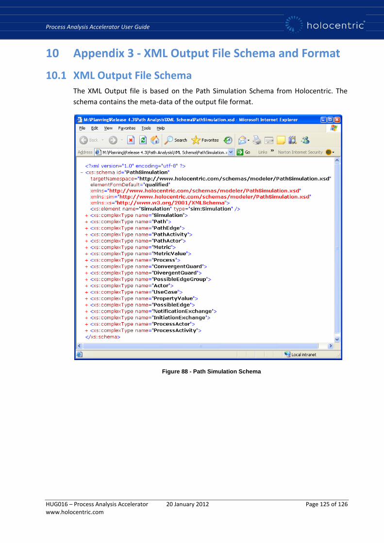
Process Analysis Accelerator User Guide
HUG016 – Process Analysis Accelerator 20 January 2012 Page 125 of 126 www.holocentric.com
10 Appendix 3 - XML Output File Schema and Format
10.1 XML Output File Schema The XML Output file is based on the Path Simulation Schema from Holocentric. The
schema contains the meta-data of the output file format.
Figure 88 - Path Simulation Schema

Process Analysis Accelerator User Guide
HUG016 – Process Analysis Accelerator 20 January 2012 Page 126 of 126 www.holocentric.com
10.2 XML Output File Example The following is an excerpt a typical output file from process analysis.
Figure 89 - Path Analysis Simulation XML Output File