radio wave diffraction and scattering models for wireless ... · radio wave diffraction and...
TRANSCRIPT

Radio Wave Diffraction and Scattering Models For
Wireless Channel Simulation
by
Mark D. Casciato
A dissertation submitted in partial fulfillmentof the requirements for the degree of
Doctor of Philosophy(Electrical Engineering)
in The University of Michigan2001
Doctoral Committee:Associate Professor Kamal Sarabandi, ChairAssociate Professor Brian GilchristProfessor Linda P.B. KatehiProfessor Thomas B.A. SeniorProfessor Wayne E. Stark

c Mark D. Casciato 2001All Rights Reserved

ACKNOWLEDGEMENTS
First I would like to acknowledge my parents, Rose and Dan Casciato for their support
throughout these last 5 years, without which attending graduate school would have been
much more difficult. I would also like to acknowledge all of my committee members,
but most especially my thesis advisor, Professor Kamal Sarabandi for his guidance and
mentorship, both academically and personally. I would also like to thank Professor Thomas
Senior for the interesting and enlightening discussions on diffraction theory. The students
and colleagues at the University of Michigan Radiation Laboratory, where to begin. I
would like to thank and acknowledge all of the students, faculty, and staff for your help
and support over my stay here at Michigan, I consider all of you good friends. I would
most especially like to thank my very close friends here, St´ephane Legault, Lee Harle,
J.D. Shumpert, Dejan Filipovich, Olgica Milenkovic, Leland Pierce, Katherine Herrick,
Mark Fischman, Dan Lawrence, Sergio Pacheco, Dimitris Peroulis, Ron Reano, Helena
Chan, Mohamed Abdelmoneum, and of course Bettina K¨othner for all the good company.
I apologize in advance for anyone that I may have missed. Finally I would like to thank the
Army Research Office for their support, without which this project would not have been
possible (contract DAAH04-96-1-037).
ii

TABLE OF CONTENTS
ACKNOWLEDGEMENTS . . . . . . . . . . . . . . . . . . . . . . . . . . . . . . ii
LIST OF TABLES . . . . . . . . . . . . . . . . . . . . . . . . . . . . . . . . . . . v
LIST OF FIGURES . . . . . . . . . . . . . . . . . . . . . . . . . . . . . . . . . . vi
LIST OF APPENDICES . . . . . . . . . . . . . . . . . . . . . . . . . . . . . . . xii
CHAPTER
1 Introduction . . . . . . . . . . . . . . . . . . . . . . . . . . . . . . . . . 11.1 Motivation . . . . . . . . . . . . . . . . . . . . . . . . . . . . . . 21.2 Research Approach . . . .. . . . . . . . . . . . . . . . . . . . . 3
1.2.1 Methodology . . .. . . . . . . . . . . . . . . . . . . . . 41.2.2 Initial Concentration . . . . . .. . . . . . . . . . . . . . 4
1.3 Relevant Assumptions & Definitions . .. . . . . . . . . . . . . . 61.4 Chapter Outline & Introduction . . . . .. . . . . . . . . . . . . . 7
2 Fields of an Infinitesimal Dipole Above an Impedance Surface: Effect ofthe Homogeneous Surface . . . . . . . . . . . . . . . . . . . . . . . . . . 10
2.1 Introduction: The Sommerfeld Problem. . . . . . . . . . . . . . 122.2 Exact Image Formulation . . . . . . . . . . . . . . . . . . . . . . 16
2.2.1 Transforms & Identities . . . . .. . . . . . . . . . . . . . 182.2.2 Vertical Electric Dipole . . . . . . . . . . . . . . . . . . . 212.2.3 Horizontal Electric Dipole . . . . . . . . . . . . . . . . . 22
2.3 Analysis & Results: Exact Image Theory . . . . . . . . . . . . . . 282.4 Chapter Summary: Exact Image Theory . . . . . . . . . . . . . . 39
3 Fields of an Infinitesimal Dipole Above an Impedance Surface: Effect ofan Impedance Transition . . . . . .. . . . . . . . . . . . . . . . . . . . . 41
3.1 Introduction: Impedance Transition . . .. . . . . . . . . . . . . . 423.2 Plane Wave Excitation . . . . . . . . . . . . . . . . . . . . . . . . 44
3.2.1 Integral Equation Formulation . . . . . . . . . . . . . . . 443.2.2 Iterative Solution .. . . . . . . . . . . . . . . . . . . . . 483.2.3 Scattered Field Expressions: Plane Wave . . .. . . . . . . 51
iii

3.2.4 Saddle Point Evaluation: Plane Wave Integral . . . . . . . 523.3 Short Dipole Excitation . . . . . . . . . . . . . . . . . . . . . . . 53
3.3.1 Stationary Phase Evaluation: Short Dipole . . . . . . . . . 543.3.2 Near-field Observation . . . . . . . . . . . . . . . . . . . 573.3.3 Error Bound . . . .. . . . . . . . . . . . . . . . . . . . . 58
3.4 Validation & Results: Perturbation Technique . . . . . . . . . . . 593.4.1 Plane Wave Excitation . . . . . . . . . . . . . . . . . . . 603.4.2 Dipole Excitation: Land/Sea Interface . . . . . . . . . . . 66
3.5 Chapter Summary: Impedance Transition. . . . . . . . . . . . . . 75
4 Diffraction from Convex Surfaces: Right Circular Cylinders .. . . . . . . 804.1 Introduction: Diffraction from Convex Surfaces . . .. . . . . . . 824.2 Development of Macromodel . . . . . .. . . . . . . . . . . . . . 86
4.2.1 Fock Theory . . . . . . . . . . . . . . . . . . . . . . . . . 884.2.2 2-D Case, Normal Incidence . . . . . . . . . . . . . . . . 904.2.3 Oblique Incidence . . . . . . . . . . . . . . . . . . . . . . 97
4.3 Validation: PEC Cylinder . . . . . . . . . . . . . . . . . . . . . . 1004.3.1 Direct Evaluation of Fock Type Integrals . . .. . . . . . . 103
4.4 Application of Macromodel. . . . . . . . . . . . . . . . . . . . . 1054.5 Other Applications . . . . . . . . . . . . . . . . . . . . . . . . . 1064.6 Chapter Summary: Diffraction from Right Circular Cylinders . . . 107
5 Diffraction from Convex Surfaces .. . . . . . . . . . . . . . . . . . . . . 1145.1 Introduction .. . . . . . . . . . . . . . . . . . . . . . . . . . . . 1155.2 Induced Surface Currents: General Convex Surface .. . . . . . . 1165.3 Results: Diffraction from Convex Surfaces . . . . . .. . . . . . . 118
5.3.1 Ellipse . . . . . . . . . . . . . . . . . . . . . . . . . . . . 1185.3.2 Knife-edge (Kirchhoff) Diffraction . . . . . .. . . . . . . 129
5.4 Chapter Summary: Diffraction from Convex Surfaces. . . . . . . 133
6 Summary & Future Work . . . . . . . . . . . . . . . . . . . . . . . . . . 1346.1 Summary: Scattering & Diffraction from Impedance Surfaces . . . 135
6.1.1 Fields of a Small Dipole Above an Impedance Surface . . 1366.1.2 Scattering from an Impedance Transition . . .. . . . . . . 136
6.2 Summary: Diffraction from Convex Surfaces . . . . .. . . . . . . 1386.3 Future Work . . . . . . . . . . . . . . . . . . . . . . . . . . . . . 139
6.3.1 Future Work: Fields of a Dipole Above an Impedance Sur-face . . . . . . . . . . . . . . . . . . . . . . . . . . . . . 140
6.3.2 Future Work: Diffraction From Convex Surfaces . . . . . . 141
APPENDICES . . . . . . . . . . . . . . . . . . . . . . . . . . . . . . . . . . . . . 142
BIBLIOGRAPHY . . . . . . . . . . . . . . . . . . . . . . . . . . . . . . . . . . . 151
iv

LIST OF TABLES
Table1.1 Soil parameters for San Antonio gray loam with a density of 1:4 g=cm3, for
varying gravimetric moisture content at 30MHz (from Hipp [1]). . . . . . . 72.1 Speed-up in computation time of exact image calculation over Sommerfeld
type integrals for normalized surface impedance of 0.3-i0.1, eleven datapoints fromD= 10! 10010m, φ= 0 and varying source/observation heights. 36
2.2 Speed-up in computation time of exact image calculation over Sommerfeldtype integrals for varying complex impedance,η. Source and receiver are2m above surface for all cases. Eleven data points are calculated fromD = 10! 10010m, φ = 0. . . . . . . . . . . . . . . . . . . . . . . . . . . 36
4.1 Optimized parameters for Sigmoidal transition functions . . .. . . . . . . 954.2 Speed-up, Macromodel to Fock Integrals . . . . .. . . . . . . . . . . . . . 104
v

LIST OF FIGURES
Figure1.1 Flowchart - Physics-based Methodology . . . . .. . . . . . . . . . . . . . 51.2 Rural Terrain Scenario. . . . . . . . . . . . . . . . . . . . . . . . . . . . 52.1 Problem geometry, dipole above an impedance plane . . . . . . . . . . . . 162.2 Exact image inz-plane . . . . . . . . . . . . . . . . . . . . . . . . . . . . 222.3 x-component of total electric fields (diffracted only for this case) for a ver-
tical (z) electric dipole, exact image (———–) compared with Sommer-feld (� � � � �). Dipole is located atx0 = y0 = 0, z0 = 2m and operating at30 MHz. Observation is atz= 2m, D = 10�10010m, along theφ = 0 (xaxis). Normalized Surface impedance value isη = 0:3� i0:1. . . . . . . . . 30
2.4 z-component of diffracted (exact image (� � � � �) and Sommerfeld (Æ Æ Æ Æ Æ))and total electric fields (exact image (———–) and Sommerfeld (� � � � ))for a vertical (z) electric dipole. Dipole is located atx0 = y0 = 0, z0 = 2mand operating at 30 MHz. Observation is atz= 2m, D = 10� 10010m,along theφ = 0 (x axis). Normalized Surface impedance value isη =0:3� i0:1. . . . . . . . . . . . . . . . . . . . . . . . . . . . . . . . . . . . 31
2.5 y-component of total electric fields for a horizontal ( ˆy) electric dipole, exactimage (———–) compared with Sommerfeld (� � � � ). Dipole islocated atx0 = y0 = 0, z0 = 2m and operating at 30 MHz. Observation isatz= 2m, D = 10�10010m, along theφ = 0 (x axis). Normalized Surfaceimpedance value isη = 0:3� i0:1. . . . . . . . . . . . . . . . . . . . . . . 33
2.6 Time (in seconds) to calculate all electric field components, at each obser-vation point, for a vertical (ˆz) electric dipole, exact image (———–) andSommerfeld (� � � � ). Dipole is located atx0 = y0 = 0, z0 = 2m andoperating at 30 MHz. Observation is atz= 2m, D = 10�10010m, alongtheφ = 0 (x axis). Normalized Surface impedance value isη = 0:3� i0:1. . 34
2.7 Time (in seconds) to calculate all electric field components, at each obser-vation point, for a horizontal ( ˆy) electric dipole, exact image (———–) andSommerfeld (� � � � ). Dipole is located atx0 = y0 = 0, z0 = 2m andoperating at 30 MHz. Observation is atz= 2m, D = 10�10010m, alongtheφ = 0 (x axis). Normalized Surface impedance value isη = 0:3� i0:1. . 35
vi
2.8 Effect of varying soil moisture onz-component of total electric fields fora vertical (z) dipole located at the origin, 2m above an impedance sur-face, (x0 = y0 = 0;z0 = 2m) and operating at 30 MHz. Observation isalso 2m above the surface and extends radially from the source along theφ = 0 (x axis) fromD = 10�10010m. Results are for soil moisture of 0%(η = 0:53, (———–)), 2.5% (η = 0:38� i0:09, (�����)), 5% (η = 0:3� i0:1,(� � � �)), 10% (η = 0:15� i0:09, (ÆÆÆÆÆ)) and 20% (η = 0:12� i0:07,(�� �� �� �)) . . . . . . . . . . . . . . . . . . . . . . . . . . . . . . . . . 37
2.9 Comparison of the magnitude of the frequency response of the direct field(———–) to total field (� � � �), for a vertical (z) dipole located at theorigin, 2.0m above the impedance surface (x0 = y0 = 0;z0= 2:0m) with realpermittivityε0r = 22:0, conductivityσ= 8�10�2. Frequency sweep is from30 to 130 MHz in steps of 142.86 KHz. Observation is also 2.0m above thesurface along theφ = 0 (x axis) and 300m from the source (D = 300m). . . 38
2.10 Comparison of the phase of the frequency response of the direct field (———–) to total field (� � � �) (in radians), for a vertical (ˆz) dipole located atthe origin, 2.0m above the impedance surface (x0 = y0 = 0;z0 = 2:0m) withreal permittivityε0r = 22:0, conductivityσ = 8�10�2. Frequency sweepis from 30 to 130 MHz in steps of 142.86. Observation is also 2.0m abovethe surface along theφ = 0 (x axis) and 300m from the source (D = 300m) 39
3.1 Scattering geometry for variable impedance surface. . . . . . .. . . . . . . 453.2 TE case, normalized bistatic echo width (σs=λ) of an impedance step insert,
5λ wide, equivalent to slightly saline water (4pp=1000 salt content,η =0:0369� i0:0308). θi = 45Æ, φi = 180Æ, first (- - - - - ) and second order(� � � � �) perturbation technique compared with GTD (———) forvarying soil moisture. . . . . . . . . . . . . . . . . . . . . . . . . . . . . . 61
3.3 TM case, normalized bistatic echo width (σs=λ) of an impedance step in-sert, 5λ wide, equivalent to slightly saline water (4pp=1000 salt content,η = 0:0369� i0:0308).θi = 45Æ, φi = 180Æ, first (- - - - -) and second order(� � � � �) perturbation technique compared with GTD (———) forvarying soil moisture. . . . . . . . . . . . . . . . . . . . . . . . . . . . . . 62
3.4 Normalized bistatic echo width, (σs=λ), of an impedance step insert ofwidth 5λ, equivalent to slightly saline water (4pp=1000 salt content,η =0:0369� i0:0308). Surrounding soil has a gravimetric moisture contendof 10% (j∆j = 0:7263). Incidence is atθi = 45Æ, first order perturbationtechnique. . . . . . . . . . . . . . . . . . . . . . . . . . . . . . . . . . . . 63
3.5 Normalized bistatic echo width, (σs=λ), of an impedance step insert ofwidth 5λ, equivalent to slightly saline water (4pp=1000 salt content,η =0:0369� i0:0308). Surrounding soil has a gravimetric moisture contend of10% (j∆j= 0:7263). Incidence is atθi = 45Æ, φi = 90Æ, first order pertur-bation technique.TETM (——–), TMTE (- - - - -). . . . . . . . . . . . . . . 64
vii

3.6 Normalized bistatic echo width, (σs=λ), of an impedance step insert ofwidth 5λ, equivalent to slightly saline water (4pp=1000 salt content,η =0:0369� i0:0308). Surrounding soil has a gravimetric moisture contendof 10% (j∆j = 0:7263). Incidence is atθi = 45Æ, φi = 180Æ, first orderperturbation technique. Step insert (——–) compared to gradual transition(- - - - -). . . . . . . . . . . . . . . . . . . . . . . . . . . . . . . . . . . . . 65
3.7 Geometry of a Land/Sea Interface . . . . . . . . . . . . . . . . . . . . . . 673.8 Magnitude (dB), Path loss, land/sea transition located atx= 0,zcomponent
of the scattered fields for a vertical (z-directed) electric dipole. Observationρ is fixed at 50λ, observationy= 0, for dipole position ofx0 =�100λ;y0 =0;z0 = 100λ. Ground moisture is 10% (ηg = 0:15� i0:09), Sea is salinewater (4pp=1000 salt content,ηw = 0:0369� i0:0308,j∆j= 1:14). Resultsfor transition widths of 0 (———), 1 (- - - - - ), and 10λ (� � � � �).Note thatψ0 = π�ψ in curves. . . . . . . . . . . . . . . . . . . . . . . . . 71
3.9 Magnitude (dB), Path loss, land/sea transition, located atx = 0, z compo-nent of the scattered fields for a vertical (z-directed) electric dipole. Tran-sition width is fixed at 1λ, observationy = 0, for dipole position ofx0 =�100λ;y0 = 0;z0 = 100λ. Ground moisture is 10% (ηg = 0:15� i0:09),Sea is saline water (4pp=1000 salt content,ηw = 0:0369� i0:0308,j∆j=1:14). Results for radial observation distanceρ of 50λ (———), 10λ (- - -- - ), and 1λ (� � � � �). Note thatψ0 = π�ψ in curves. . . . . . . . . . 72
3.10 Magnitude (dB), Path loss, land/sea transition, located atx = 0, z com-ponent of the scattered fields for a vertical (z-directed) electric dipole.Transition width is fixed at 1λ, Radial observationρ is fixed at 10λ, forvaryingy offset between source and observation (oblique incidence), andfor dipole position ofx0 = �100λ;z0 = 100λ. Ground moisture is 10%(ηg = 0:15� i0:09), Sea is saline water (4pp=1000 salt content,ηw =0:0369� i0:0308, j∆j = 1:14). Results for offset iny of 0 (———), 50(- - - - - ), and 100λ (� � � � �). Note thatψ0 = π�ψ in curves. . . . . . 73
3.11 Magnitude (dB), Path loss, land/sea transition, located atx = 0, z com-ponent of the scattered fields for a vertical (z-directed) electric dipole.Transition width is 0λ (abrupt), observationy = 0, observationx from�50λ to 150λ. Dipole position is atx0 = �100λ;y0 = 0λ. for varyingsource/observation heights. Ground moisture is 10% (ηg = 0:15� i0:09),Sea is saline water (4pp=1000 salt content,ηw = 0:0369� i0:0308,j∆j=1:14). Results for space wave (———), and total dipole fields (- - - - - ). . . 77
3.12 Magnitude (dB), Path loss, land/sea transition, located atx = 0, z compo-nent of the scattered fields for a vertical (z-directed) electric dipole. Tran-sition width is 0λ (abrupt), observationy = 0, observationx from �50λto 150λ. Dipole position is atx0 = �100λ;y0 = 0λ. Source/observationheightz0 = z= 1λ. Ground moisture is 10% (ηg = 0:15� i0:09), Sea issaline water (4pp=1000 salt content,ηw = 0:0369� i0:0308,j∆j= 1:14).Results for space wave (———), total dipole fields, infinite transition func-tion (- - - - - ), total dipole fields, weighted transition function (� � � � �). 78
viii

3.13 Magnitude(dB), Path loss, land/sea transition, located atx = 0, z compo-nent of the scattered fields for a vertical (z-directed) electric dipole. Tran-sition width is 0λ (abrupt), observationx from �50λ to 150λ, observa-tion y from �50λ to 50λ. Dipole position is atx0 = �100λ;y0 = 0λ.Source/observation are atz0 = z= 1λ. Ground moisture is 10% (ηg =0:15� i0:09), Sea is saline water (4pp=1000 salt content,ηw = 0:0369�i0:0308,j∆j= 1:14). . . . . . . . . . . . . . . . . . . . . . . . . . . . . . 79
4.1 Definition of regions around a convex surface. . .. . . . . . . . . . . . . . 834.2 Scattering geometry of an infinite cylinder. . . . . . . . . . . . . . . . . . . 874.3 Diffraction current magnitude (dB) around full circumference of 10 and
100λ PEC cylinders excited at normal incidence angle,θi = π=2, eigenso-lution current (———–), compared with macromodeled current (- - - - - -),φ2π = 0 is equivalent to a point on top of the cylinder, perpendicular to the
shadow boundary, withφ2π =�0:25 in the deep shadow region. . . . . . . . 1014.4 Gentle phase component (degrees) around full circumference of 10 and
100λ PEC cylinders excited at normal incidence angle,θi = π=2, 10λ (———–), 100λ (- - - - - -), φ
2π = 0 is equivalent to a point on top of the
cylinder, perpendicular to the shadow boundary, withφ2π = �0:25 in the
deep shadow region. . . . . . . . . . . . . . . . . . . . . . . . . . . . . . 1024.5 Total current, magnitude (dB) and phase (degrees) around full circumfer-
ence of a 100λ PEC cylinder excited at oblique incidence angle,θi = π=4,eigensolution current (———–), compared with macromodeled current (-- - - - -), φ
2π = 0 is equivalent to a point on top of the cylinder, perpendicular
to the shadow boundary, withφ2π = �0:25 in the deep shadow region. (a)and (b) are magnitude and phase of TMz - directed current with (c) and (d)magnitude of TEφ andz - directed current respectively. . . . .. . . . . . . 109
4.6 Magnitude (dB) of total E-fields 1λ off the surface of a 100λ PEC cylinderexcited by a plane wave at oblique incidence angle,θi = π=4, eigensolu-tion (———–), macromodel (- -- - - -) with �90Æ corresponding to deepshadow and 90Æ corresponding to normal incidence (deep lit). .. . . . . . . 110
4.7 Total current magnitude (dB) of Fock currents around full circumferenceof a PEC cylinder excited at normal incidence angle,θi = π=2, a = 10λ(———–), a= 15λ (- - - - - -), a= 20λ (� � � � �). φ
2π = 0 is equivalentto a point on top of the cylinder, perpendicular to the shadow boundary,with φ
2π =�0:25 in the deep shadow region. . . . . . . . . . . . . . . . . . 1114.8 Magnitude (dB) of total TM E-fields 1λ off the surface of a 15λ PEC cylin-
der excited by a plane wave at normal incidencdθi = π=2, macromodel(———–), Fock integrals (- - - - - -) with�90Æ corresponding to deepshadow and 90Æ corresponding to normal incidence (deep lit). .. . . . . . . 112
ix

4.9 Magnitude (dB) of total far-fields generated by a point source (small dipole)radiating in the presence of a 20λ PEC cylinder positioned 0:1λ off cylindersurface along thex axis (0Æ in plot) at z= 0. Observation is at 2(2a)2=λfrom cylinder center and inx� y plane atz= 0, eigensolution (———–),macromodel (- - - - - -). . . . . . . . . . . . . . . . . . . . . . . . . . . . 113
5.1 Ridgelines in Mountainous Region .. . . . . . . . . . . . . . . . . . . . . 1155.2 Geometry of a General Convex Surface . . . . .. . . . . . . . . . . . . . 1165.3 Geometry of Elliptical Cylinder . .. . . . . . . . . . . . . . . . . . . . . 1195.4 Magnitude (dB), total fields 1λ off the surface of an ellipse, with y-dimension
a= 10λ, x-dimensionb= 8λ. Incidence angleφi is at 90Æ, MoM solution(———–), compared with macromodel (- - - - - -). . . . . . . . . . . . . . 121
5.5 Magnitude (dB), total fields 1λ off the surface of an ellipse, with y-dimensiona= 8λ, x-dimensionb= 10λ. Incidence angleφi is at 90Æ, MoM solution(———–), compared with macromodel (- - - - - -). . . . . . . . . . . . . . 122
5.6 Magnitude (dB), total fields 1λ off the surface of an ellipse, with y-dimensiona= 10λ, x-dimensionb= 5λ. Incidence angleφi is at 90Æ, MoM solution(———–), compared with macromodel (- - - - - -). . . . . . . . . . . . . . 123
5.7 Magnitude (dB), total fields 1λ off the surface of an ellipse, with y-dimensiona= 5λ, x-dimensionb= 10λ. Incidence angleφi is at 90Æ, MoM solution(———–), compared with macromodel (- - - - - -). . . . . . . . . . . . . . 124
5.8 Magnitude (dB), total fields 1λ off the surface of an ellipse, with y-dimensiona= 10λ, x-dimensionb= 3:33λ. Incidence angleφi is at 90Æ, MoM solu-tion (———–), compared with macromodel (- - - - - -). . . . . . . . . . . . 125
5.9 Magnitude (dB), total fields 1λ off the surface of an ellipse, with y-dimensiona= 10λ, x-dimensionb= 2:5λ. Incidence angleφi is at 90Æ, MoM solution(———–), compared with macromodel (- - - - - -). . . . . . . . . . . . . . 126
5.10 Magnitude (dB), total fields 1λ off the surface of an ellipse, with y-dimensiona= 10λ, x-dimensionb= 8λ. Incidence angleφi is at 45Æ, MoM solution(———–), compared with macromodel (- - - - - -). . . . . . . . . . . . . . 127
5.11 Magnitude (dB), total fields 1λ off the surface of an ellipse, with y-dimensiona= 8λ, x-dimensionb= 10λ. Incidence angleφi is at 45Æ, MoM solution(———–), compared with macromodel (- - - - - -). . . . . . . . . . . . . . 128
5.12 Scattering Geometry, Knife-edge and Convex Surface . . . . .. . . . . . . 1305.13 Path loss (dB), total fields from an obstacle of heighth= 50λ, and width
w = 6λ. Observation is aty = �51λ and incident angle is atφi = 90Æ
(normal to the screen). Macromodel (———–), compared with knife-edge(Kirchhoff) diffraction (- - - - - -). . . . . . . . . . . . . . . . . . . . . . . 131
5.14 Path loss (dB), total fields from an obstacle of heighth= 50λ, and widthw = 50λ. Observation is aty = �51λ and incident angle is atφi = 90Æ
(normal to the screen). Macromodel (———–), compared with knife-edge(Kirchhoff) diffraction (- - - - - -). . . . . . . . . . . . . . . . . . . . . . . 132
x

5.15 Path loss (dB), total fields from an obstacle of heighth= 50λ, and widthw = 100λ. Observation is aty = �51λ and incident angle is atφi = 90Æ
(normal to the screen). Macromodel (———–), compared with knife-edge(Kirchhoff) diffraction (- - - - - -). . . . . . . . . . . . . . . . . . . . . . . 132
A.1 Problem geometry, dipole above an impedance plane . . . . . . . . . . . . 144B.1 Scattering geometry for variable impedance surface. . . . . . .. . . . . . . 149
xi

LIST OF APPENDICES
AppendixA Alternate Spectral Domain Representation the Fields of a Small Dipole
Above an Impedance Half-Space . . . . . . . . . . . . . . . . . . . . . . . 143B Derivation of 2-D Dyadic Green’s Function . . .. . . . . . . . . . . . . . 148
xii

CHAPTER 1
Introduction
The propagation of a radio wave through some physical environment is effected by
various mechanisms which affect the fidelity of the received signal. Accurate prediction
of these effects is essential in the design and development of a communications system.
These effects can include shadowing and diffraction caused by obstacles along the prop-
agation path, such as hills or mountains in a rural area, or buildings in a more urban en-
vironment. Reflections off obstacles or the ground cause multi-path effects and the radio
signal can be significantly attenuated by various environmental factors such as ionospheric
effects, propagation through vegetation, such as in a forest environment, or reflection from
an impedance transition such as a river or land/sea interface. When line-of-sight (LOS)
propagation is not present these environmental mechanisms have the dominate effect on
the fidelity of the received signal through dispersive effects, fading, and signal attenuation.
Accurate prediction of these propagation effects allow the communications system en-
gineer to address the trade-off between radiated power and signal processing by developing
an optimum system configuration in terms of modulation schemes, coding, frequency band
and bandwidth, antenna design, and power. Current techniques commonly applied to char-
acterizing the communications channel are highly heuristic in nature and not generally
applicable. It is the intent of this work to define a methodology for the accurate and general
prediction of radio wave propagation by application of electromagnetic wave theory, and
1

within this framework to develop electromagnetic models of canonical geometries which
represent various scattering and diffraction mechanisms in the propagation environment.
The scope of the problem should not be underestimated and once a basic methodology
is defined initial research must be narrowed to a specific region of investigation, i.e., fre-
quency band, domain type (rural, urban, satellite-based, ground-based, etc). These initial
electromagnetic models can then be built upon as a bases for expansion of the overall model
to include a wider range of propagation scenarios.
In the sections that follow the previous discussion will be expanded upon. The motiva-
tion behind this work is first discussed. Next the research approach is detailed, with a basic
methodology for the prediction of radio wave propagation defined. The specific focus of
this thesis within the broader scope of the propagation problem is then given, including a
description of two canonical diffraction models developed. The next section contains rel-
evant conventions, definitions and assumptions, used throughout this thesis, followed by a
brief introduction and outline of the chapters that follow.
1.1 Motivation
The basic motivating factor behind this work is the need for development of an accurate
and general propagation model. As mentioned previously the ability to accurately predict
the effects of the propagation environment on a communications channel is essential in the
development and optimal design of a communications system. Current methods of channel
characterization, while having the advantage of simplicity, do not adequately address the
issue and there is a need for significant improvement in the prediction of radio wave prop-
agation. Commonly used methods of channel characterization can be broken down into
two areas, empirical models, which are highly heuristic in nature, and simplified analytic
models. The empirical models are constructed from measured data and are not directly
connected to the physical processes involved. This limits them to very specific environ-
2
mental conditions at the time the measurements were made as well as measurement system
attributes (band, bandwidth, and polarization). An example of a commonly used empirical
model for urban environments is the Okumura model [2]. This model uses simple alge-
braic equations to calculate mean path-loss for fixed frequency, observation distance, and
transmitter/receiver height. It does not account for coherence bandwidth, fading, or de-
polarization effects. In addition it fails if the antenna heights or orientations are changed.
Analytic models, while attempting to account for the interaction of the various mechanisms
which effect propagation, are simplified to a degree as to make them invalid for most prac-
tical applications. An example of this is the Longley-Rice irregular terrain model [3]. It
uses Geometrical Optics (GO) and ray-tracing to account for reflected fields and knife-edge
or Kirchhoff diffraction to account for path obstacles. The GO approximation does not ac-
count for shadowing and the knife-edge approximation is invalid in the transition region
between light and shadow and in the shadow region.
Due to the discussed shortcomings in existing methods of propagation prediction a
more rigorous approach, based on the application of electromagnetic wave theory, must be
applied to the problem at hand. The approach to be defined is directly connected to the
physical processes at work in the propagation environment and will result in propagation
models which are both accurate and more generally applicable.
1.2 Research Approach
As stated the prediction of radio wave propagation for general environments and in an
accurate manner is a complex problem with many avenues of research to pursue. In this
section a general approach or methodology for developing a complete propagation model is
defined. Within this framework the canonical models developed in this thesis are described.
3

1.2.1 Methodology
The development of a more accurate and general model to predict radio wave prop-
agation requires that a basic methodology or approach to the problem be defined. The
flowchart in Figure 1.1 outlines this basic approach. Referring to Figure 1.1, the prob-
lem is first defined in terms of regions or domains, each of which have their own unique
environmental characteristics, thus requiring a somewhat different (although sometimes
overlapping) approach to solving the subsequent electromagnetic problem. These regions
can be defined in terms of urban/rural domains or ground-based/satellite-based scenarios.
The basic methodology within these domains is to develop a set of canonical diffraction
and scattering models which represent various environmental features. These models are
developed using the technique most appropriate for the given electromagnetic problem, i.e.,
analytic, numeric or some type of hybrid technique. Approximations are made which allow
for efficient application of the model, while retaining the accuracy required. The individ-
ual models are then merged into a complete propagation scenario. Monte Carlo simulation
accounts for the statistical nature of the propagation channel. Eventually remote sensing
information obtained from available databases can be used to define the propagation envi-
ronment. The complete model will allow for a simulation which is directly based on the
physical environment and therefore accurate and generally applicable.
1.2.2 Initial Concentration
Having defined the basic methodology to developing an overall propagation model an
area of concentration is now defined for this initial research. In this work the investigation
is focused on the rural domain or environment and ground-based (point to point) or ground
to/from unmanned aerial vehicle (UAV) communication at frequencies from HF through
L-Band. Figure 1.2 shows a typical propagation environment in a rural area. The radio
wave can be diffracted by obstacles such as hills, or mountains or an impedance transition
4

Physics Based Approximations, Improve Computational Efficiency, Retain Accuracy
Incorporate into Physical Model of Propagation Environment for EM Simulation
Hybrid Analytical/Numerical Diffraction Models RepresentingVarious Rural, Urban &
Atmospheric Features
Satellite Geographical /Environmental Database
Analytical Models, Canonical Shapes Only
Numerical Solutions,Computationally Intensive
Integrate Diffraction Models to Predict Relevant Interactions
Geographical Database
Environmental Features and Statistics, Rural, Urban and Atmospheric
Merge Environmental Model and Integrated Diffraction Model into Accurate EM Propagation Model
Accurate Mean-field, Coherency, Variance, Polarization Effects, Multi-path & Dispersion (Delay) Effects
Figure 1.1: Flowchart - Physics-based Methodology
such as a river or land/sea interface. Along the propagation path the signal may be per-
turbed by a highly scattering medium such as a forest. In this work two diffraction models
are developed, based on canonical geometries, and applicable to a rural environment, for
eventual integration into the overall propagation model. The first represents the effects of
a flat earth on the radio signal, which can contain a one-dimensional impedance variation,
representative of a river or land/sea interface. The second calculates the effects on the radio
signal of singly curved, convex obstacles with a large, slowly varying radius of curvature,
and which can represent terrain features such as hills or mountains.
Figure 1.2: Rural Terrain Scenario
5

1.3 Relevant Assumptions & Definitions
In this section relevant assumptions, definitions, and conventions are given. Unless
otherwise indicated they are valid throughout the thesis.
The time conventione�iωt is assumed throughout this thesis and suppressed.
It is assumed throughout that the effects of the Earth can be modeled as a highly con-
ductive, non-magnetic impedance surface (εr ! ∞; µr = 1), which is essentially impen-
etrable and the Standard Impedance Boundary Condition (SIBC), namely,(n� n�E) =
�Z(n�H), with Z being the impedance of the Earth, is applied throughout. This as-
sumption is valid for a lossy Earth where the penetration depth, d, is small (d � λ), and
is applicable at the frequencies of interest in this work. Interested readers are referred to
[4] for a discussion on the SIBC as well as techniques to improve on the accuracy of this
assumption.
As the intent is to represent a lossy Earth in a realistic fashion, impedance values are
chosen which are representative of moist earth, or in the case of propagation over water,
saline water. The impedance values of the soil are derived from the values of permittivity
and conductivity given by Hipp [1] for San Antonio Gray Loam with a density of 1:4 g=cm3
and a varying moisture content (given as percent moisture in terms of gravimetric moisture
content). The impedance values of the water are derived from the equations for complex
permittivity given by Ulaby, et al., for saline water, with a salt content defined as as parts
per 1000 on a weight basis (pp/1000) [5]. Table 1.1 shows the complex permittivity and
conductivity calculated from the tables in [1] for San Antonio gray loam with moisture
content varying from 0 to 20%. Many of the examples to be shown are in the HF to VHF
frequency range, and as the permittivity and conductivity values in Table 1.1 are essentially
unvarying over this range the values given are assumed to be constant across this frequency
band.
It should also be noted that all simulation results provided in this thesis were run on a
Sun Microsystems Ultra2, with a 300MHz Sun microprocessor.
6

Table 1.1: Soil parameters for San Antonio gray loam with a density of 1:4 g=cm3, forvarying gravimetric moisture content at 30MHz (from Hipp [1]).
% Moisture ε0r σ0:0 3:5 � 10�4
2:5 5:8 5:0�10�3
5:0 8:2 1:0�10�2
10:0 14:0 5:0�10�2
20:0 24:0 8:0�10�2
1.4 Chapter Outline & Introduction
In the chapters that follow the development of the aforementioned diffraction models
along with relevant results and applications are presented. Each of these models represents
an independent electromagnetic problem and therefore each chapter, or a group of chapters
for each model is somewhat self-contained. The basic format is as follows. Each chapter
will contain brief paragraphs at the beginning and end to maintain a continuity or flow
from chapter to chapter. Each chapter will begin with an introductory section. This section
will include a detailed history and background of the problem at hand, the most current
techniques being applied, and the motivation for further research into improving on these,
or developing new techniques. Following this introduction will be a section containing the
specifics of the diffraction model being developed, including formulations and appropriate
derivations. A section containing validation and results follows. The final section in each
chapter will summarize the chapter and draw conclusions.
A problem of significant interest is the propagation of radio waves over a lossy Earth.
The surface of the Earth can be modeled locally as a flat, impedance half-space which can
also contain some type of transition in the surface impedance such as caused by a river or
seashore. In Chapters 2 and 3 a diffraction model for an impedance half-space, with one-
dimensional impedance variation, when excited by an infinitesimal dipole, is developed. In
Chapter 2 the effects of the homogeneous surface, without the transition is accounted for.
7
This is a form of the classic Sommerfeld problem of the fields of an infinitesimal dipole
radiating above an lossy half-space. Resulting field expressions contain Sommerfeld type
integrals, which are highly oscillatory, and difficult to evaluate numerically. In Chapter 2 a
method is developed to transform the Sommerfeld integrals into a form more conducive to
numerical evaluation, while retaining the rigor of the original expressions. Beginning with
an alternate spectral domain representation of the dipole fields, an integral transform tech-
nique known as exact image theory is applied. Resulting field expressions are exact, and
contain integrands which converge extremely rapidly, up to several orders of magnitude
faster than the original Sommerfeld expressions. To complete the model for propagation
above an impedance half-space, Chapter 3 addresses the effect of an impedance transition
in the surface. Current methods such as the Geometrical Theory of Diffraction (GTD) can
only account for the effect of an abrupt discontinuity in the surface impedance. In Chap-
ter 3 a method is developed which is valid for any arbitrary one dimensional impedance
transition in the surface, provided the Fourier transform of the surface impedance function
is known. By application of a perturbation technique, an integral equation is solved for
unknown surface currents. Resulting expressions for the surface currents are recursive in
orders of perturbation in terms of multi-fold convolution. Far-field expressions are alge-
braic to first order. Also in Chapter 3 the combined effects of both the homogeneous surface
and the impedance transition are analyzed. Analysis of a land/sea transition shows that the
effects of the transition on the total fields is significant when both source and observation
are near the surface and insensitive to the gradient of the transition.
Another problem of significant interest is that of the propagation of radio waves over
convex obstacles encountered in the propagation environment such as hills, mountains, or
ridgelines. Current methods applied to this problem include Kirchhoff (knife-edge) diffrac-
tion, whose shortcomings have already been discussed, and GTD methods for both wedge
and convex surfaces. Solutions for wedge diffraction require a local radius of curvature
smaller than 1/100 of a wavelength which does not occur in nature, even at HF frequencies.
8

GTD methods for convex surfaces tend to be mathematically and numerically cumbersome
and no one GTD method is valid in all regions around the surface (near-field, far-field, deep
shadow, deep lit, transition regions between light and shadow). In Chapters 4 and 5 a model
is developed which calculates the scattering and diffraction from a singly-curved convex
surface, with large slowly varying radius of curvature. The initial model is developed for
a perfect electric conducting (PEC) surface and determines induced surface currents in a
highly accurate fashion. Unlike GTD techniques for convex surfaces the technique requires
no numerical integration or complex mathematical analysis to determine these currents. For
a convex surface with large, slowly varying radius of curvature, the induced surface cur-
rents can be approximated locally by those of a circular cylinder and the solution of this
canonical problem is the first step in developing a model of the induced surface currents on
a general convex surface. In Chapter 4, a macromodel for the induced surface currents on
a circular PEC cylinder, when excited by a plane wave at oblique incidence, is first devel-
oped. This macromodel of the surface currents is based on the definitions of the Physical
Theory of Diffraction (PTD) [6] in which the total surface currents are decomposed into a
uniform, or physical optics (PO) component and a non-uniform or diffraction component,
which is a correction to the PO solution. Application of this macromodel produces highly
accurate surface currents for cylinders of any radius above one wavelength. This current is
generated by a simple scaling and interpolation of the exact currents on a reference cylinder
of moderate radius. In Chapter 5, the method is extended to general, singly-curved, convex
surfaces using existing methods found in the literature. The model is first applied to an el-
liptical cylinder and compared with results from a Method of Moments (MoM) numerical
code. The model is then applied to a parabolic surface and results are compared to those
generated by applying Kirchhoff (knife-edge) diffraction techniques.
In Chapter 6 this thesis work is summarized and conclusions drawn as well as sugges-
tions for future work.
9

CHAPTER 2
Fields of an Infinitesimal Dipole Above an Impedance
Surface: Effect of the Homogeneous Surface
In this chapter and the next the effects of a lossy earth on the fields of an infinitesimal
dipole are examined. These effects can be modeled locally as a flat, planar, impedance
surface and the surface can contain an impedance transition such as a river or sea/land in-
terface. The problem can be decomposed into the effect of the homogeneous surface and
the effect caused by some impedance transition in the surface such as would be caused by
a river, sea/land interface, or swamp/dry land transition. In this chapter the effect of the ho-
mogeneous surface on the dipole fields is first discussed, with the effect of the impedance
transition as well as the combined effect of the homogeneous surface and impedance transi-
tion analyzed in the next. In order to avoid confusion, in the next two chapters the following
terminologies are adopted: The effect of the homogeneous surface on the total dipole fields
will be referred to as the diffracted fields, while the effect of the impedance transition is
defined as the scattered fields.
Calculation of the fields of an infinitesimal dipole radiating above a homogeneous
impedance half-space is a form of the classic Sommerfeld problem of calculating the fields
of an infinitesimal dipole above a lossy half-space. A solution to this problem was first
formulated by Arnold Sommerfeld in 1909 [7] and the resulting expressions for the tra-
10

ditional solution consist of integrals of the Sommerfeld type which cannot be evaluated
in closed form and due to their highly oscillatory nature are difficult to evaluate numeri-
cally. A form of these integrals is thus sought, which retains the rigor and generality of
the original formulation, while making them more conducive to numerical computation.
By application of an integral transform method known as exact image theory explicit ex-
pressions are derived for a dipole of arbitrary orientation, above an impedance surface. A
spectral domain representation of the dipole fields, of a form not previously seen in the
literature, is first given. To apply exact image theory the reflection coefficients of the spec-
tral domain representation are cast in the form of the Laplace transform of an exponential
function. By exchanging the order of integration, the spectral domain integration is per-
formed analytically and field expressions are obtained which consist of rapidly converging
integrals in the Laplace domain. As no approximations are made, these expressions are
exact, and valid for any arbitrary source alignment or observation position. It is shown
that the formulation for a horizontal dipole contains an image in the conjugate complex
plane resulting in a diverging exponential term not previously discussed in the literature.
Comparison of numerical results from exact image theory and the original Sommerfeld type
expressions shows good agreement as well as a speed-up in computation time of several or-
ders of magnitude, which depends on the distance between the transmitter and the receiver.
This formulation can effectively replace the approximate asymptotic expressions used for
predicting wave propagation over a smooth planar ground (having different regions of va-
lidity) and in conjunction with the techniques of Chapter 3 (diffraction from an impedance
surface with one-dimensional impedance transition) provides a complete methodology for
the analysis of radio wave propagation over a smooth planar ground which can contain a
general, one-dimensional impedance transition.
11

2.1 Introduction: The Sommerfeld Problem
The problem of a infinitesimal electric dipole radiating above a lossy half-space was
originally formulated by Arnold Sommerfeld in his classic work published in 1909 [7].
Since then it is an understatement to say that this problem has received a significant amount
of attention in the literature, with literally hundreds of papers published on the subject. The
inclusion of a sign error in the original work prompted much debate, over several decades,
on the existence of a Zenneck type surface wave and its significance in the fields generated
by a vertical electric dipole. The complete history of the problem is beyond the scope of this
thesis, but suffice to say that independent derivations by Weyl [8], Sommerfeld [9], van der
Pol and Niessen, [10] and Wise [11] confirmed the sign error, although Sommerfeld himself
never admitted to any error in the original 1909 work. The corrected formulation confirmed
the existence of a surface wave for certain values of impedance and observation angles, but
showed its contribution to the total field only significant within a certain range of distances,
dependent on the impedance of the half-space (Sommerfeld numerical distance). Readers
are referred to the work of Norton [12, 13] for a concise formulation of the problem, with
correct sign, and Ba˜nos [14] for a complete perspective of the historical development of the
mathematics of the problem.
The Sommerfeld solution is expressed in terms of integrals which cannot be evaluated
in closed form and due to their highly oscillatory nature are difficult to evaluate numeri-
cally. Numerous techniques, both analytic and numeric, have been applied to evaluate the
Sommerfeld integrals in an approximate fashion. To evaluate the Sommerfeld integrals an-
alytically standard asymptotic techniques, such as the method of steepest descent (Saddle
Point method), are typically applied [15, 16]. These techniques are valid when distance
between source and observation is large and contributions from poles (surface wave) and
branch cuts (lateral wave) must be accounted for when deforming the contour. For source
and observation near the surface the direct and reflected waves (geometrical optics (GO)
term, first order Saddle point) tend to cancel and higher order terms in the asymptotic ex-
12

pansion are dominate. Norton interpreted this effect as a type of surface wave and thus
these higher order terms are typically referred to in the literature as a Norton Surface Wave
[12, 13]. For a highly lossy surface (small normalized impedance) the pole approaches the
saddle point and their contributions cannot be separated. In this case standard saddle point
techniques cannot be applied and an alternate asymptotic technique is necessary [15, 16].
To evaluate the Sommerfeld type integrals numerically, in an approximate fashion, several
techniques have been proposed. Parhamiet. al [17] proposed a method, valid for a vertical
electric dipole, in which the integration contour is deformed to the steepest descent path.
The integral is then solved asymptotically when distance between image and observation
is large, and numerically when this distance is small. Again poles and branch cuts must be
accounted for when the contour deformation encounters them and the technique requires
evaluation of Hankel functions of complex argument. Michalski [18] improved on this
method by proposing a variation in the way a branch cut is handled. Johnson and Dudley
[19] proposed a method, valid for small distances between image and observation, in which
an analytic technique is applied to reduce the oscillatory nature of the Sommerfeld inte-
grand. While these techniques improve the convergence properties of the Sommerfeld type
integrals they require transformations which increase the complexity of the formulation
and, as in the case of the asymptotic solutions, are not valid for all source and observation
positions, and electrical parameters.
As none of these analytical/numerical techniques are valid for general source orienta-
tion and observation location, or arbitrary impedance values, a solution is sought which
transforms the Sommerfeld type expressions into a form which retains the rigor and gener-
ality of the original formulation, while improving the computational efficiency to a degree
which makes evaluation of the resulting exact expressions practical from a numerical stand-
point. In order to improve the convergence properties of the Sommerfeld type integrals, an
integral transform technique known as exact image theory is applied. In this method an in-
tegral transform, in the form of the Laplace transform of an exponential function, is applied
13

to the reflection coefficients of the Sommerfeld type integrals, resulting in expressions now
consisting of a double integral, one in the original spectral domain and one in the Laplace
domain. Application of appropriate identities allows for analytical evaluation of the integral
in the spectral domain and the remaining integral expressions in the Laplace domain are
dominated by a rapidly decaying exponential. These integral expressions are exact, with no
approximations made and the decaying exponential in the integrand results in significantly
improved convergence properties over the original formulation. The form of these integral
expressions can be interpreted as a distributed line source, located at the image point of the
dipole source, and extending into the complex plane.
Evaluating the Sommerfeld expressions as a type of distributed image was first pro-
posed by Booker and Clemmow [20]. They recognized that the first order term in the
asymptotic expansion of the field expressions in the upper half-space for a vertical dipole
was equivalent to straight edge (Kirchhoff) diffraction around a half-screen, if the screen
extended from the physical image point, vertically to infinity (in the upper half-space). The
field distribution in the lower half-space was in the form of a Fresnel type integral and could
be interpreted as a distributed line source beginning at the same physical image point and
extending to infinity in the lower half space. Representation of the reflection coefficients in
the Sommerfeld formulation in terms of the Laplace transform of an exponential function,
for a vertical electric dipole, was apparently first introduced by van der Pol [21] and can
also be seen in the work of Norton and Furutsu [13, 22]. Their intent in applying this type
of integral transformation was to simplify the asymptotic evaluation of the Sommerfeld
formulation by modifying the integrand into a more well behaved form. Interpretation of
this modified form of the integrand, for a vertical electric dipole, as a distributed image
source located in the complex plane was apparently first proposed by Felsen and Marcuvitz
[15], who recognized the improved convergence properties of the integrand for numerical
computation. Lindell and Alanen extended the technique to that of electric and magnetic
dipoles of arbitrary orientation radiating above a dielectric half-space [23, 24, 25]. For the
14

dielectric case there is no exact transform for the reflection coefficient and the formulation
by Lindell and Alanen for the vertical electric dipole involves a decomposition of the kernel
function of the Laplace transform. For the case of a horizontal electric dipole only a formal
solution is presented, with no explicit expressions or detailed interpretation of image be-
havior. This might have been due to the fact that for a general half-space dielectric medium
exact analytical expressions for the image currents do not exist. However, such expressions
can be obtained for impedance surfaces and the behavior of the image currents for arbitrary
dipole orientation can be studied.
In this chapter exact image theory is applied to the problem of an electric dipole, of
arbitrary orientation, radiating above an impedance half-space. In Section 2.2 a spectral
domain representation of a form not previously seen in the literature, is given for the dipole
electric fields. For interested readers the derivation of this spectral form can be found in
Appendix A. This representation of the dipole fields, which consists of integrals of the
Sommerfeld type, is the starting point for all derivations that follow. Appropriate Bessel
identities are then given which are needed to transform the spectral domain representation
into a form which contains Bessel functions of the first kind, of order zero only, an initial
step in the derivation. The case of a vertical electric dipole is first examined, in a manner
similar to that of Felsen and Marcuvitz [15]. The methodology is then extended to the case
of a horizontal electric dipole, where it is noted that duality cannot be applied to solve the
equivalent problem of a vertical magnetic dipole radiating above a impedance surface. As
mentioned, integral expressions for the horizontal dipole show a diverging exponential term
which is not apparent in the formulation by Lindell and Alanen for a dielectric half-space
[25]. In Section 2.3 results are given including a comparison of field quantities generated by
evaluation of the exact image integrals, and the original Sommerfeld type expressions. In
addition a timing comparison shows numerical evaluation of the exact image formulation
to be several orders of magnitude faster than numerical evaluation of the corresponding
Sommerfeld type integrals. In Section 2.4 the chapter is summarized.
15

2.2 Exact Image Formulation
Consider the problem geometry shown in Figure 2.1. A small dipole of lengthl , car-
●
Z1
φ
D
-z
z
z
x
y
Observation
R
θ
k ,Z 00
I l0
0
0
0
Figure 2.1: Problem geometry, dipole above an impedance plane
rying currentI0 and with orientationl is radiating in free space above an infinite, homo-
geneous impedance plane, representative of a lossy Earth. The characteristic impedance
of free space and of the impedance plane are defined asZ0 andZ1, respectively. The total
fields above the impedance plane propagate with the propagation constant of free spacek0,
and can be decomposed into a direct wave and diffracted wave given by
ET(r ; r0) = Ei(r ; r0)+Ed(r ; r0); (2.1)
wherer =p
x2+y2+z2 is the distance to the observation point andr0 =p
x02+y0
2+z02
is the distance to the source location. Also in (2.1) superscriptsT, i andd are indicative of
the total, direct and diffracted fields respectively, the diffracted fields being the perturbation
in the total fields caused by the impedance half-space.Ei(r ; r0) can be calculated directly
and the expression for it is given in Appendix A. Of interest are the diffracted fields and
16

we begin the exact image derivation with an alternate spectral domain representation of the
dipole fields. As the focus of this work is the transformation of the this representation into
a form more conducive to numerical evaluation, the derivation will not be repeated here.
Interested readers are referred to Appendix A for an explicit derivation of these expressions.
The spectral representation of the diffracted electric fields of a dipole of orientationl , where
l = lxx+ lyy+ lzz, located at the origin, and radiating above an infinite impedance plane are
given by
Ed(r ; r0) =k0Z0I0l
4π
�x
∞Z
0
kρ
2kzfΓh[�lx(J2(kρD)cos2φ+J0(kρD))� lyJ2(kρD)sin2φ)]
+Γv[2ikzkρ
k20
lzcosφJ1(kρD)+k2
z
k20
lx(J0(kρD)�J2(kρD)cos2φ)
�k2z
k20
lyJ2(kρD)sin2φ]g eikz(z+z0) dkρ
+y
∞Z
0
kρ
2kzfΓh[�lxJ2(kρD)sin2φ� ly(J0(kρD)�J2(kρD)cos2φ)]
+Γv[2ikzkρ
k20
lzsinφJ1(kρD)� k2z
k20
lxJ2(kρD)sin2φ
+k2
z
k20
ly(J0(kρD)+J2(kρD)cos2φ)]g eikz(z+z0) dkρ
�z
∞Z
0
kρ
kzΓv[
k2ρ
k20
lzJ0(kρD)+ikzkρ
k20
(lxcosφ
+lysinφ)J1(kρD)] eikz(z+z0) dkρ
�;
(2.2)
whereΓh and Γv are the horizontal (TE toz) and vertical (TM toz) Fresnel reflection
coefficients, respectively, given by
Γh =η�k0=kz
η+k0=kz; Γv =
�η+kz=k0
η+kz=k0; (2.3)
17

andη = Z1=Z0, is the normalized impedance of the half-space. In (2.2)kz is the dependent
variable defined ask2z = k2
0�k2ρ, andJ0;J1, andJ2 are Bessel functions of the first kind, of
order 0;1, and 2 respectively. Also in (2.2)D defines the radial distance between source
and observation points,z the height of the observation point,φ is the angle betweenD and
thex axis, withz0 being the height of the source point, all of which are seen in Figure 2.1.
The integrals in (2.2) are Sommerfeld type integrals and as already stated they are
highly oscillatory in nature, with poor convergence properties making them difficult to
evaluate numerically, especially for the case ofD� (z+z0). To improve the convergence
behavior of these integrals exact image theory is applied, by the application of integral
transforms and appropriate identities. The method is exact with no approximations made
and the resulting expressions are valid for any arbitrary source and observation position.
The basic methodology is to first rewrite the spectral domain formulation of (2.2) in terms
of zeroth order Bessel functions of the first kind only. Terms containing reflection coef-
ficients in the resulting expressions are expanded where necessary, and then rewritten in
the simple form of the Laplace transform of an exponential function. Order of integration
is exchanged and the spectral domain integration overkρ in (2.2) is performed in an an-
alytic fashion. The remaining expressions in the Laplace domain contain integrals which
are dominated by rapidly decaying exponentials and exhibit significantly improved con-
vergence properties over the original Sommerfeld expressions. In the next section relevant
transforms and identities will be given that are needed for the derivations that follow.
2.2.1 Transforms & Identities
In this section transforms and identities which are used throughout the derivations that
follow are defined. To apply exact image theoryΓh andΓv, given in (2.3), must be defined
in terms of a Laplace transform of an exponential function.Γh andΓv can be rewritten as,
Γh = 1� 2k0=ηkz+k0=η
= 1� 2κkz+κ
; (2.4)
18

whereκ = k0=η, and
Γv = 1� 2ηk0
kz+ηk0= 1� 2γ
kz+ γ; (2.5)
whereγ = ηk0. Now recognizing that
∞Z
0
e�ζξ e�kzξ dξ =1
kz+ζ; (2.6)
whereζ is some constant coefficient, we can rewriteΓh andΓv in the form of a Laplace
transform of an exponential function or,
Γh = 1�2κ∞Z
0
e�(κ+kz)ξ dξ; (2.7)
and
Γv = 1�2γ∞Z
0
e�(γ+kz)ξ dξ: (2.8)
In the application of exact image theory to the case of a horizontal dipole, several terms
arise in the derivation which containΓh andΓv, however cannot be directly expressed as the
Laplace transform defined in (2.6). For the sake of simplicity and in order to minimize the
complexity of the resulting expressions it is desirable that all integral transforms applied
be in the form of this Laplace transform. For a horizontal dipole this is accomplished by
expanding the terms, where necessary, by partial fractions into a form which allows them
to be directly written in the form of (2.6).
In applying exact image theory to the Sommerfeld type expressions for the fields of
a dipole above an impedance surface an initial step in the derivation is to apply Bessel
function identities in order to rewrite (2.2) in terms ofJ0 only. To do this the following
19

identities are needed:
1
k20
∂2
∂x2J0(kρD) =� k2ρ
2k20
[J0(kρD)�cos2φJ2(kρD)]; (2.9)
1
k20
∂2
∂y2J0(kρD) =� k2ρ
2k20
[J0(kρD)+cos2φJ2(kρD)]; (2.10)
1
k20
�∂2
∂x2 +∂2
∂y2
�J0(kρD) =�k2
ρ
k20
J0(kρD); (2.11)
1
k20
∂2
∂x∂yJ0(kρD) =
k2ρ
2k20
sin2φJ2(kρD); (2.12)
1
k20
∂2
∂x∂zJ0(kρD) =�i cosφ
kzkρ
k20
J1(kρD); (2.13)
1
k20
∂2
∂y∂zJ0(kρD) =�i sinφ
kzkρ
k20
J1(kρD): (2.14)
An additional identity which will allows for the analytic evaluation of the spectral do-
main integrals overkρ in the exact image expressions is
eik0R
R= i
∞Z
0
J0(kρD) eikz(z+z0)kρ
kzdkρ; (2.15)
whereR=p
(x�x0)2+(y�y0)2+(z+z0)2. The identity in (2.15) relates the free space
Green’s function to an alternate representation in the form of a Sommerfeld integral and is
appropriately referred to in the literature as the Sommerfeld Integral Identity.
20
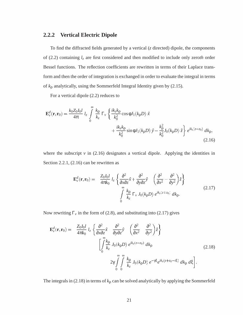
2.2.2 Vertical Electric Dipole
To find the diffracted fields generated by a vertical (z directed) dipole, the components
of (2.2) containinglz are first considered and then modified to include only zeroth order
Bessel functions. The reflection coefficients are rewritten in terms of their Laplace trans-
form and then the order of integration is exchanged in order to evaluate the integral in terms
of kρ analytically, using the Sommerfeld Integral Identity given by (2.15).
For a vertical dipole (2.2) reduces to
Edv(r ; r0) =
k0Z0I0l4π
lz
∞Z
0
kρ
kzΓv
�ikzkρ
k20
cosφJ1(kρD) x
+ikzkρ
k20
sinφJ1(kρD) y� k2ρ
k20J0(kρD) z
�eikz(z+z0) dkρ;
(2.16)
where the subscriptv in (2.16) designates a vertical dipole. Applying the identities in
Section 2.2.1, (2.16) can be rewritten as
Edv(r ; r0) =�Z0I0l
4πk0lz
�∂2
∂x∂zx+
∂2
∂y∂zy�
�∂2
∂x2 +∂2
∂y2
�z
�∞Z
0
kρ
kzΓv J0(kρD) eikz(z+z0) dkρ:
(2.17)
Now rewritingΓv in the form of (2.8), and substituting into (2.17) gives
Edv(r ; r0) =�Z0I0l
4πk0lz
�∂2
∂x∂zx+
∂2
∂y∂zy�
�∂2
∂x2 +∂2
∂y2
�z
�� ∞Z
0
kρ
kzJ0(kρD) eikz(z+z0) dkρ
�2γ∞Z
0
∞Z
0
kρ
kzJ0(kρD) e�γξeikz(z+z0+iξ) dkρ dξ
�:
(2.18)
The integrals in (2.18) in terms ofkρ can be solved analytically by applying the Sommerfeld
21

integral identity of (2.15), giving the final form of the diffracted electric fields for a vertical
(z directed) dipole
Edv(r ; r0) =
iZ0I0l4πk0
lz
�∂2
∂x∂zx+
∂2
∂y∂zy�
�∂2
∂x2 +∂2
∂y2
�z
��
eik0R
R�2γ
∞Z
0
e�γξ eik0R0(ξ)
R0(ξ)dξ�;
(2.19)
whereR is as previously defined andR0(ξ) =p
(x�x0)2+(y�y0)2+(z+z0+ iξ)2. The
integrand in the last term of (2.19) can be interpreted as a distributed image source in the
complexzplane located at�z0, and as seen in Figure 2.2. In this integrand both exponential
factors,�γξ, and�k0R0(ξ), decay rapidly asξ becomes large. Due to this, the integral in
(2.19) converges very rapidly, for all source and observation locations.
Im[z]
Re[z]
z - plane
-z
e-γξ
ξ
|I |image
0
Figure 2.2: Exact image inz-plane
2.2.3 Horizontal Electric Dipole
Before beginning the derivation of the fields from a horizontal electric dipole a brief
note about the application of duality is relevant. Having solved the problem of the elec-
tric fields from a vertical electric dipole above an impedance half-space, the problem of
22

the magnetic fields of a vertical magnetic dipole above a similar half-space can be im-
mediately written by applying duality. Through Maxwell’s equations, electric fields are
obtained, equivalent to those generated by a loop of electric current in thex�y plane, and
it would appear at first glance that a solution which gives some insight into the problem of
a horizontal electric dipole is at hand. Several problems arise however. First it is desired
to obtain accurate dipole fields for any dipole orientation and observation and information
about the effects of the dipole pattern are lost in the dual solution. Also in applying dual-
ity the case of an impedance surface is transformed to that of an admittance surface, which
gives little physical insight into the problem. Because of these issues, the case of a horizon-
tal dielectric dipole radiating above an impedance half-space will be derived directly. As
the scalar potential is not obvious in the expressions for a horizontal dipole, the derivation
to be presented, while somewhat more cumbersome algebraically, results in complete field
expressions in terms of the exact image formulation for arbitrary dipole orientation in the
x�y plane.
In a manner similar to that of the vertical dipole appropriate terms in the Sommerfeld
type expressions for a horizontal dipole will be put in terms ofJ0 only to facilitate eval-
uation of the integral overkρ analytically. Initially thex component of the electric field
is derived. They component is determined in the same fashion, which for brevity will
not be repeated, and only the final result is provided. Finally thez component of the field
generated by a horizontal electric dipole is derived.
To derive thex component of the diffracted electric field for a horizontal electric dipole
the identities of (2.9) through (2.14) are applied, and noting thatk2z = k2
0� k2ρ, (2.2), be-
23

comes
Edh(r ; r0) � x= k0Z0I0l
4π
∞Z
0
�lxk2
ρ
�Γh
∂2
∂y2 �Γvk2
0�k2ρ
k20
∂2
∂x2
�
� lyk2
ρ
�Γh+Γv
k20�k2
ρ
k20
�∂2
∂x∂y
�kρ
kzJ0(kρD) eikz(z+z0)dkρ;
(2.20)
where the subscripth designates a horizontal dipole. (2.20) can be rewritten as
Edh(r ; r0) � x= k0Z0I0l
4π
�lx(
∂2
∂y2 fa� ∂2
∂x2 fb+1
k20
∂2
∂x2 fc)
�ly∂2
∂x∂y( fa+ fb� 1
k20
fc)
�;
(2.21)
where
fa =
∞Z
0
kρ
kzJ0(kρD) eikz(z+z0)
Γh
k2ρ
dkρ; (2.22)
fb =
∞Z
0
kρ
kzJ0(kρD) eikz(z+z0)
Γv
k2ρ
dkρ; (2.23)
and
fc =
∞Z
0
kρ
kzJ0(kρD) eikz(z+z0) Γv dkρ: (2.24)
While fc can be evaluated directly by expressingΓv in the form of (2.8) (as in the previous
section, eqns. (2.17), (2.18), and (2.19)), the termsΓh=k2ρ andΓv=k2
ρ, in fa; and fb, cannot
be directly written in terms of the Laplace transform of (2.6), however by applying partial
24

fraction expansion they can be put in the appropriate form. Defining these terms as
A=Γh
k2ρ; B=
Γv
k2ρ; (2.25)
writing Γh andΓv explicitly in terms ofk0; kz; κ, andγ (see (2.4) and (2.5)), and recognizing
thatk2ρ = k2
0�k2z = (k0�kz)(k0+kz), A andB can be written as
A=kz�κ
(k0�kz)(k0+kz)(kz+κ); (2.26)
and
B=kz� γ
(k0�kz)(k0+kz)(kz+ γ): (2.27)
Expanding (2.26) and (2.27) by partial fractions gives expressions of the following form
for A andB
A=A1
(k0�kz)+
A2
(k0+kz)+
A3
(kz+κ); (2.28)
B=B1
(k0�kz)+
B2
(k0+kz)+
B3
(kz+ γ); (2.29)
where
A1 =�B1 =η�1
2k0(η+1);
A2 =�B2 =η+1
2k0(η�1);
A3 =�B3 =2η
k0(1�η2);
(2.30)
25

and where the coefficients in (2.30) are given explicitly in terms of normalized impedance
η andk0, which will be used in the final expressions for thex component of the diffracted
electric fields. Now representing each term of the partial fraction expansions of (2.28) and
(2.29) in the form of the Laplace transform of (2.6), changing the order of integration as
before and applying (2.15) to evaluate the integral overkρ analytically, gives the following
expressions forfa and fb
fa =�i
∞Z
0
�e�k0ξ (A1
eik0R00(ξ)
R00(ξ)+A2
eik0R0(ξ)
R0(ξ))+A3 e�κξ eik0R0(ξ)
R0(ξ)
�dξ; (2.31)
fb =�i
∞Z
0
�e�k0ξ (B1
eik0R00(ξ)
R00(ξ)+B2
eik0R0(ξ)
R0(ξ))+B3 e�γξ eik0R0(ξ)
R0(ξ)
�dξ; (2.32)
whereR00(ξ) =p
(x�x0)2+(y�y0)2+(z+z0� iξ)2. Also the expression forfc is given
by
fc =�i
�eik0R
R�2γ
∞Z
0
e�γξ eik0R0(ξ)
R0(ξ)dξ�: (2.33)
26
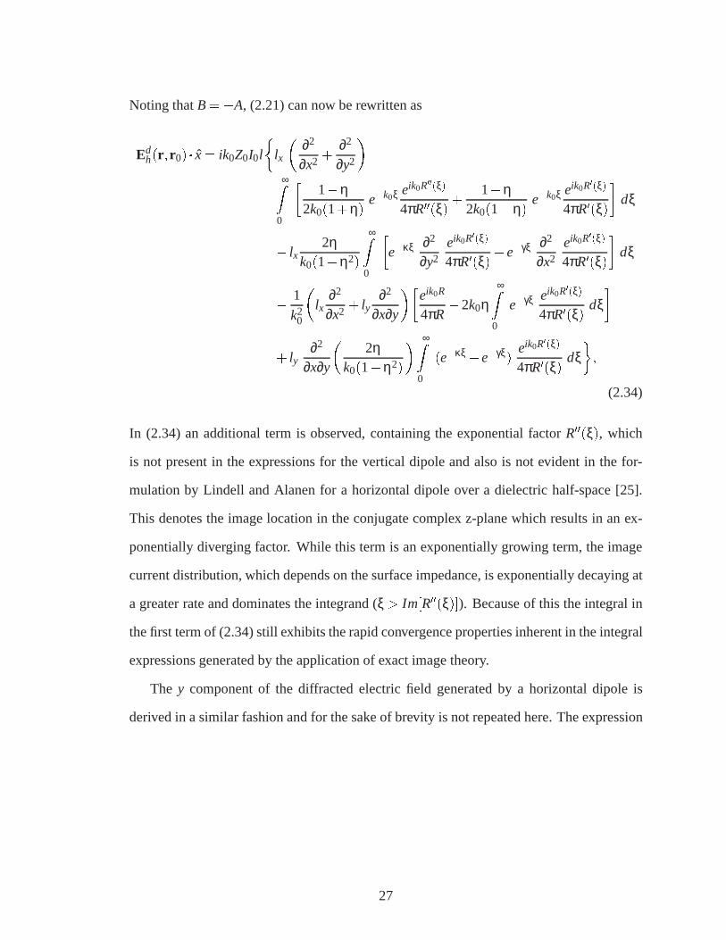
Noting thatB=�A, (2.21) can now be rewritten as
Edh(r ; r0) ��� x= ik0Z0I0l
�lx
�∂2
∂x2 +∂2
∂y2
�∞Z
0
�1�η
2k0(1+η)e�k0ξ eik0R00(ξ)
4πR00(ξ)+
1+η2k0(1�η)
e�k0ξ eik0R0(ξ)
4πR0(ξ)
�dξ
� lx2η
k0(1�η2)
∞Z
0
�e�κξ ∂2
∂y2
eik0R0(ξ)
4πR0(ξ)+e�γξ ∂2
∂x2
eik0R0(ξ)
4πR0(ξ)
�dξ
� 1
k20
�lx
∂2
∂x2 + ly∂2
∂x∂y
��eik0R
4πR�2k0η
∞Z
0
e�γξ eik0R0(ξ)
4πR0(ξ)dξ�
+ ly∂2
∂x∂y
�2η
k0(1�η2)
� ∞Z
0
(e�κξ�e�γξ)eik0R0(ξ)
4πR0(ξ)dξ�;
(2.34)
In (2.34) an additional term is observed, containing the exponential factorR00(ξ), which
is not present in the expressions for the vertical dipole and also is not evident in the for-
mulation by Lindell and Alanen for a horizontal dipole over a dielectric half-space [25].
This denotes the image location in the conjugate complex z-plane which results in an ex-
ponentially diverging factor. While this term is an exponentially growing term, the image
current distribution, which depends on the surface impedance, is exponentially decaying at
a greater rate and dominates the integrand (ξ > Im[R00(ξ)]). Because of this the integral in
the first term of (2.34) still exhibits the rapid convergence properties inherent in the integral
expressions generated by the application of exact image theory.
The y component of the diffracted electric field generated by a horizontal dipole is
derived in a similar fashion and for the sake of brevity is not repeated here. The expression
27

for it is given by
Edh(r ; r0) ��� y= ik0Z0I0l
�ly
�∂2
∂x2 +∂2
∂y2
�∞Z
0
�1�η
2k0(1+η)e�k0ξ eik0R00(ξ)
4πR00(ξ)+
1+η2k0(1�η)
e�k0ξ eik0R0(ξ)
4πR0(ξ)
�dξ
� ly2η
k0(1�η2)
∞Z
0
�e�κξ ∂2
∂x2
eik0R0(ξ)
4πR0(ξ)+e�γξ ∂2
∂y2
eik0R0(ξ)
4πR0(ξ)
�dξ
� 1
k20
�ly
∂2
∂y2 + lx∂2
∂x∂y
��eik0R
4πR�2k0η
∞Z
0
e�γξ eik0R0(ξ)
4πR0(ξ)dξ�
+ lx∂2
∂x∂y
�2η
k0(1�η2)
� ∞Z
0
(e�κξ�e�γξ)eik0R0(ξ)
4πR0(ξ)dξ�:
(2.35)
Derivation of thez component of the diffracted electric field generated by a horizontal
dipole is rather straightforward. Beginning with (2.2) and applying the appropriate identi-
ties we arrive at
Edh(r ; r0) � z= 1
k20
(lx∂2
∂x∂z+ ly
∂2
∂y∂z)
∞Z
0
kρ
kzΓv J0 eikz(z+z0) dkρ; (2.36)
and recognizing the integral in (2.36) asfc, thez component of the electric field generated
by a horizontal dipole is given by
Edh(r ; r0) � z=�ik0Z0I0l
�1
k20
(lx∂2
∂x∂z+ ly
∂2
∂y∂z)
�eik0R
4πR�2γ
∞Z
0
e�γξ eik0R0(ξ)
4πR0(ξ)dξ��
:
(2.37)
2.3 Analysis & Results: Exact Image Theory
In this section a validation of the exact image method will be given, along with timing
results showing the significant speed-up in computation time over that of the original Som-
28

merfeld type expressions. In the results that follow all integrals are numerically evaluated
using the Gaussian quadrature numerical integration package Quadpack contained in the
Slatec mathematical computation libraries. The Quadpack routines require defining both
an absolute and relative error parameter, and these were set at 0:0 and 0:001 respectively.
For the initial comparison of the exact image formulation to the original Sommerfeld
type expressions, consider an electric dipole located 2m above the impedance surface (z0 =
2m), at the coordinate origin (x0 = y0 = 0) and radiating at 30 MHz. All field quantities are
normalized to dipole lengthl , currentI0 and wavelengthλ (E=(I0l=λ)), for all cases. The
geometry and coordinates are again as shown in Figure 2.1. The observation is on a radial
line, 2m above the impedance surface (z= 2m), ranging from 10m to 10010m along thex
axis (D = 10! 10010m; φ = 0) and field values are calculated at 11 data points along this
line. The normalized surface impedance value is chosen to beη = 0:3� i0:1 corresponding
to the impedance of San Antonio Gray Clay Loam with a 5% gravimetric moisture content
and a density of 1:4 g=cm3, derived from the values of permittivity and conductivity given
by Hipp [1], and as shown in Table 1.1.
Figure 2.3 shows thex component of the diffracted electric field, for a vertical dipole,
for this test case (no directx field component in this case). In Figure 2.3 results from nu-
merical evaluation of the exact image expressions are compared to results from numerical
evaluation of the original Sommerfeld type expressions. As can be seen the two results
are in excellent agreement. For the same test case Figure 2.4 shows the diffracted and total
(direct + diffracted)zelectric field components for a vertical (zdirected) dipole, again com-
paring the exact image calculation to those of the Sommerfeld formulation. As can be seen
in Figure 2.4 the diffracted fields are in good agreement, except for a slight discrepancy at
4000m, where evaluation of the Sommerfeld type integrals did not completely converge.
The total fields in Figure 2.4 show increased error at 4000m for the Sommerfeld solution
and also at distances beyond 6000m. This is due to the fact that the total field is the result
of two large numbers (direct and diffracted field) tending to cancel, for source and obser-
29

0 2000 4000 6000 8000 10000−100
−80
−60
−40
−20
0
20
40
ρ (meters)
|Ex
| (dB
)
D
Figure 2.3:x-component of total electric fields (diffracted only for this case) for a vertical(z) electric dipole, exact image (———–) compared with Sommerfeld (�����).Dipole is located atx0 = y0 = 0,z0 = 2mand operating at 30 MHz. Observationis atz= 2m, D = 10�10010m, along theφ = 0 (x axis). Normalized Surfaceimpedance value isη = 0:3� i0:1.
vation near the impedance surface. This has the effect of highlighting the numerical error
in the Sommerfeld integrals for the diffracted field, while the curves generated by the exact
image formulation decay smoothly as expected, thus indicating better convergence in the
numerical solution. This in fact is the case where higher order terms (Norton surface wave)
in the approximate asymptotic solutions dominate the total fields forR� (z+z0). To eval-
uate the effects of the Norton surface wave we observe that the expression forfc given in
(2.24) is simply thez directed potential for a vertical dipole. Defining this potential asGz,
the asymptotic solution ofGz can be decomposed as
Gz = Giz+Ggo
z +Gnswz (2.38)
where superscripti indicates the direct wave,go is the Geometrical Optics (GO) term,
30

0 2000 4000 6000 8000 10000−100
−80
−60
−40
−20
0
20
40
ρ (meters)
|Ez
| (dB
)
D
Figure 2.4:z-component of diffracted (exact image (� � � � �) and Sommerfeld (Æ Æ Æ Æ Æ)) andtotal electric fields (exact image (———–) and Sommerfeld (� � � � ))for a vertical (z) electric dipole. Dipole is located atx0 = y0 = 0, z0 = 2m andoperating at 30 MHz. Observation is atz= 2m, D = 10�10010m, along theφ = 0 (x axis). Normalized Surface impedance value isη = 0:3� i0:1.
equivalent to the first order Saddle point solution, andnsw indicates the Norton surface
wave component of the asymptotic solution, which is simply the higher order terms in the
Saddle point expansion, and which decay as 1=R2. The first two terms in (2.38) are given
by
Giz+Ggo
z =eik0R0
4πR0+Γv;sp
eik0R
4πR(2.39)
whereR0 =p
(x�x0)2+(y�y0)2+(z�z0)2 andΓv;sp is the vertical Fresnel reflection
coefficient evaluated at the saddle point, and given by
Γv;sp=cosθ0�ηcosθ0+η
: (2.40)
31

In (2.40) cosθ0 = (z+ z0)=R, andθ0 is as defined in Figure 2.1. Equation (2.39) can be
rewritten as
Gz =eik0R0
4πR0� eik0R
4πR+
2cosθ0
cosθ0+η; (2.41)
As source and observation move near the impedance surface the first two terms in (2.41)
tend to cancel and terms which decay as 1=ρ2 tend to dominate. These terms are implicit
in the third term of (2.41) and the higher order terms of the asymptotic expansion (Norton
surface wave). Assuming thatjηj � cosθ0, expanding (2.41) in a Taylor series, and rep-
resenting cosθ0 in terms ofz, z0, andρ, the decay as 1=ρ2 as well as the dependence of
(2.41) onη become explicit and (2.41) now becomes
Giz+Ggo
z =1
2πρ2 (�ik0zz0+z+z0
η) eik0ρ; (2.42)
where in (2.42) it is assumed that a pole is not in the vicinity of the saddle point. Again
assuming thatjηj � cosθ0, the higher order terms in the asymptotic expansion (Norton
surface wave) are given by,
Gnswz =
p�i8πk0ρ2
�14� 4
η2
�eik0ρ: (2.43)
Figure 2.5 shows they components of the total electric field for a horizontal (y directed)
dipole, and for the same test case. Again the convergence problems of the Sommerfeld
type integrals are apparent in Figure 2.5 in the degradation of the appropriate curve beyond
2000m.
Having compared the accuracy of the exact image formulation to that of the original
Sommerfeld expressions the significant improvement in computational time will now be
discussed. In Figure 2.6 and Figure 2.7 the computation time (in seconds), required to cal-
culate all field components at each observation point is plotted for this same test case. The
32

0 2000 4000 6000 8000 10000−100
−80
−60
−40
−20
0
20
40
ρ (meters)
|Ey
| (dB
)
D
Figure 2.5:y-component of total electric fields for a horizontal ( ˆy) electric dipole, exactimage (———–) compared with Sommerfeld (� � � � ). Dipole is locatedat x0 = y0 = 0, z0 = 2m and operating at 30 MHz. Observation is atz= 2m,D = 10� 10010m, along theφ = 0 (x axis). Normalized Surface impedancevalue isη = 0:3� i0:1.
curves in Figure 2.6 compare the time required for numerical evaluation of the Sommerfeld
type solution for the case of a vertical dipole, to the time required for the exact image for-
mulation to perform the same field calculations. Figure 2.7 shows a similar comparison for
a horizontal (y directed) electric dipole. As is obvious from both sets of curves, the com-
putation time required for the exact image calculations are significantly faster than the time
required to calculate the Sommerfeld integrals, in fact over two orders of magnitude faster
as the observation distance goes beyond 2000m. Note that for both methods only necessary
integrals were evaluated, i.e., for example, the integrals containinglx were not called if
the dipole was strictlyz directed (lz component only). In continuing with a comparison of
computation time between exact image and the Sommerfeld integrals, Table 2.1 shows a
comparison of the speed-up in computation time required by the exact image formulation
33

0 2000 4000 6000 8000 1000010
−2
10−1
100
101
102
ρ (meters)
Exe
cutio
n tim
e (s
econ
ds)
D
Figure 2.6: Time (in seconds) to calculate all electric field components, at each observationpoint, for a vertical (ˆz) electric dipole, exact image (———–) and Sommerfeld(� � � � ). Dipole is located atx0 = y0 = 0, z0 = 2m and operating at30 MHz. Observation is atz= 2m, D = 10�10010m, along theφ = 0 (x axis).Normalized Surface impedance value isη = 0:3� i0:1.
over the original Sommerfeld type expressions. Speed-up is defined as the ratio of the time
required to calculate the Sommerfeld expressions to that required to perform the exact im-
age calculations (Sommerfeld time (seconds)/ exact image time (seconds)). In Table 2.1 the
computation time for each method is the time required to calculate all field components at
all observation positions (still eleven data points, fromD= 10! 10010m, φ = 0), again for
the case ofη = 0:3� i0:1, but with varying source and observation heights. As is seen in
Table 2.1 the exact image calculations exhibit a significant speed-up in convergence time,
over the Sommerfeld type expression, for numerical evaluation of the integrals. As a final
comparison of computation times, Table 2.2 shows the speed-up in computation time of
the exact image formulation over the Sommerfeld type expressions, for varying normal-
ized complex impedance values and for eleven data points, fromD = 10! 10010m, φ = 0,
34

0 2000 4000 6000 8000 1000010
−2
10−1
100
101
102
ρ (meters)
Exe
cutio
n tim
e (s
econ
ds)
D
Figure 2.7: Time (in seconds) to calculate all electric field components, at each observationpoint, for a horizontal ( ˆy) electric dipole, exact image (———–) and Sommer-feld (� � � � ). Dipole is located atx0 = y0 = 0, z0 = 2m and operating at30 MHz. Observation is atz= 2m, D = 10�10010m, along theφ = 0 (x axis).Normalized Surface impedance value isη = 0:3� i0:1.
and for source and observation 2m above the impedance surface. Again the exact image
calculations are at least an order of magnitude faster than the Sommerfeld calculations for
all cases except that of a PEC surface.
Also in this section the effects of varying soil moisture on the total electric fields of a
vertical dipole, are presented. The dipole is again radiating at 30 MHz, with source 2m
above the impedance surface, observation is also 2m above the impedance surface, and
again along thex axis fromD = 10 toD = 10010m. Figure 2.8 shows a comparison of the
z component of the total electric fields, calculated using the exact image expressions, for
the same San Antonio Gray Clay Loam previously described, and again with a density of
1:4g=cm3. The curves show field levels for gravimetric moisture contents of 0%, 2.5%, 5%,
10%, and 20%, corresponding to normalized surface impedances (η) of 0:53, 0:38� i0:09,
35

Table 2.1: Speed-up in computation time of exact image calculation over Sommerfeld typeintegrals for normalized surface impedance of 0.3-i0.1, eleven data points fromD = 10! 10010m, φ = 0 and varying source/observation heights.
z0(m) z(m) Speed-up, Vertical Dipole Speed-up, Horizontal Dipole2 2 303.92 565.962 200 54.89 106.92
200 2 56.11 107.00200 200 65.00 110.00
Table 2.2: Speed-up in computation time of exact image calculation over Sommerfeld typeintegrals for varying complex impedance,η. Source and receiver are 2m abovesurface for all cases. Eleven data points are calculated fromD = 10! 10010m,φ = 0.
η Speed-up, Vertical Dipole Speed-up, Horizontal Dipole0.0-i0.0 5.41 13.860.1-i0.0 282.00 613.800.3-i0.0 318.17 624.600.5-i0.0 490.38 715.92
0.003-i0.1 9.81 31.030.003-i0.3 10.03 18.30.003-i0.5 9.96 14.510.1-i0.1 254.29 425.620.3-i0.3 266.00 452.200.5-i0.5 348.25 510.28
0:3� i0:1, 0:15� i0:09, 0:12� i0:07, respectively. As can be seen in Figure 2.8 the effect
of increasing moisture content (η is decreased) is to increase the vertical component of the
total electric fields by as much as 20 dB over the range shown. This dependence onη can
be seen in the asymptotic form of the fields ((2.42)). A similar analysis for a horizontal
dipole (y directed and again observation along thex axis) showed the total field levels to be
essentially insensitive to varying soil moisture.
As a final example the frequency response of the field of a vertical dipole over the
impedance half-space is examined. The frequency response is indicative of the dispersive
effects of the half-space, and these effects are of significant interest in the point to point
36

0 2000 4000 6000 8000 10000−100
−80
−60
−40
−20
0
20
40
ρ (meters)
|Ez
| (dB
)
D
Figure 2.8: Effect of varying soil moisture onz-component of total electric fields for avertical (z) dipole located at the origin, 2m above an impedance surface, (x0 =y0 = 0;z0 = 2m) and operating at 30 MHz. Observation is also 2m above thesurface and extends radially from the source along theφ = 0 (x axis) fromD = 10�10010m. Results are for soil moisture of 0% (η = 0:53, (———–)),2.5% (η = 0:38� i0:09, (�����)), 5% (η = 0:3� i0:1, (� � � �)), 10% (η =0:15� i0:09, (ÆÆÆÆÆ)) and 20% (η = 0:12� i0:07, (�� �� �� �))
transmission of wideband radio signals over the earth. For this example the source and ob-
servation are placed 2mabove the surface and the frequency response is examined at radial
distanceD = 300m from the source. Frequency is swept from 30 MHz to 130 MHz in steps
of 142.86 KHz. For obvious reasons the electric field quantities are not normalized toI0l=λ
as in the previous examples. Also field expressions must be multiplied by the dipole length
(in meters), and in this example the length is set at 0:2307m (λ=10 at 130MHz). As the
normalized impedance of the surface varies with frequency, the appropriate real compo-
nent of the relative permittivity (ε0r ) and conductivity (σ) are selected from the tables given
by Hipp [1] (Table 1.1) and the normalized impedance calculated from these parameters
at each frequency. As previously mentioned these values are slowing varying functions of
37

frequency so the values given in Table 1.1, are assumed to be constant across the band.
The normalized impedance,η, at each frequency is then given byη = 1=p
ε0r + iε00r , where
ε00r = σ=(ωε0) andε0 = 8:85� 10�12 is the permittivity of free space. For this example
these values were again chosen to be representative of San Antonio Gray Clay Loam with a
20% gravimetric moisture content and a density of 1:4 g=cm3 (ε0r = 24:0 andσ = 8�10�2
in Table 1.1). Figure 2.9 and Figure 2.10 compare the magnitude and phase of the fre-
quency response of the direct dipole field to that of the total field. It is shown that the
30 40 50 60 70 80 90 100 110 120 130−50
−45
−40
−35
−30
−25
−20
Frequency (MHz)
|Ez| (
dB)
Figure 2.9: Comparison of the magnitude of the frequency response of the direct field(———–) to total field (� � � �), for a vertical (z) dipole located at theorigin, 2.0m above the impedance surface (x0 = y0 = 0;z0 = 2:0m) with realpermittivity ε0r = 22:0, conductivityσ = 8� 10�2. Frequency sweep is from30 to 130 MHz in steps of 142.86 KHz. Observation is also 2.0m above thesurface along theφ = 0 (x axis) and 300m from the source (D = 300m).
magnitude of the frequency response for the total field is monotonic and slowing varying
while the phase is essentially linear and almost identical to the phase of the direct field.
The phase behavior indicates that there is little or no dispersion of the broadband signal in
38

30 40 50 60 70 80 90 100 110 120 1300
100
200
300
400
500
600
700
Frequency (MHz)
∠ E
z (R
adia
ns)
Figure 2.10: Comparison of the phase of the frequency response of the direct field(———–) to total field (� � � �) (in radians), for a vertical (ˆz) dipolelocated at the origin, 2.0m above the impedance surface (x0 = y0 = 0;z0 =2:0m) with real permittivityε0r = 22:0, conductivityσ = 8�10�2. Frequencysweep is from 30 to 130 MHz in steps of 142.86. Observation is also2.0m above the surface along theφ = 0 (x axis) and 300m from the source(D = 300m)
such communications channels. This was found to be true for various complex impedances
corresponding to different moisture content, with the exception of the case of either source
or observation raised above the surface to a point where there is a significant difference in
path delay between the direct and ground (diffracted) waves.
2.4 Chapter Summary: Exact Image Theory
In this chapter the effects of a lossy, homogeneous flat earth on a propagating radio wave
was analyzed. Starting with a spectral domain representation of the fields of an infinitesi-
mal dipole above an impedance half space, the highly oscillatory Sommerfeld type integrals
39

inherent in the original formulation, were transformed into a form more conducive to nu-
merical computation. By application of exact image theory, the convergence properties of
these integrals are improved to a degree making them practical for numerical computation
in their rigorous form. The Sommerfeld expressions are written in terms of zeroth order
Bessel functions of the first kind, and the reflection coefficients cast in the form of a simple
Laplace transform of an exponential function. Where necessary terms are expanded by par-
tial fractions so they can be expressed in this form. Order of integration is then exchanged
and the inverse transform from the spectral domain performed analytically. The remaining
expressions consist of integrals whose integrand is dominated by a decaying exponential,
and exhibit rapid convergence qualities. Numerical evaluation of these integrals show good
agreement with results obtained by numerical evaluation of the Sommerfeld type integrals,
while exhibiting a speed up in computation time of several orders of magnitude.
Having formulated a practical method for the efficient and accurate calculation of the
dipole fields above a homogeneous impedance surface, it is now desired to include the
effects of an impedance transition as might be caused by a river or land/sea interface in a
locally flat earth. In the next chapter this effect is accounted for by applying a perturbation
technique in the Fourier domain to solve for unknown surface currents. The method to
be described in Chapter 3 is valid for any general one-dimensional impedance transition,
where the Fourier transform of the impedance transition function exists.
40

CHAPTER 3
Fields of an Infinitesimal Dipole Above an Impedance
Surface: Effect of an Impedance Transition
In the previous chapter the effects of a homogeneous impedance surface on the fields
of an infinitesimal dipole were determined in a more efficient fashion by application of
exact image theory to the original spectral domain expressions, in the form of Sommerfeld
type integrals. In this chapter the model is extended to account for the effects of a general
one-dimensional impedance transition on the dipole fields. This transition in an otherwise
homogeneous surface can be representative of a river, trough, or land/sea interface. The
problem of plane wave excitation is first solved and then extended to that of dipole exci-
tation in the standard way by representation of the dipole fields as a continuous spectrum
of plane waves. To derive the model an integral equation is first formulated in the Fourier
domain, and then solved iteratively using a perturbation technique. An analytical solution
is provided to any desired order in terms of multi-fold convolution integrals of the Fourier
transform of the impedance function. For far-field observation the resulting integrals are
solved by applying standard saddle point techniques, resulting in expressions for the in-
duced surface currents which are algebraic to first order in the perturbation series. Also, an
error bound for the perturbation parameter is established and defined in terms of incident
wave polarization and angle. The method is first validated by comparison with Geometri-
41
cal Theory of Diffraction (GTD) techniques for an abrupt impedance transition (step insert)
and plane wave excitation. Effects of varying both the width of the insert and perturbation
parameter of the insert are discussed as well as the effect of oblique incidence and a more
gradual transition on the scattered fields. The technique is then integrated with that of the
previous chapter for a homogeneous surface, and the effect of a seashore or land/sea tran-
sition on the total fields of an infinitesimal dipole are examined. Note that, as previously
discussed, the effect of the transition on the total dipole fields is defined as the scattered
fields, while the effects of the homogeneous surface is defined as the diffracted fields.
3.1 Introduction: Impedance Transition
In order to completely characterize the fields of an infinitesimal dipole above a lossy
Earth, the effects of any impedance transition or inhomogeneity, such as caused by a river
or land/sea interface must be accounted for. For non-canonical problems it is usually dif-
ficult to obtain exact solutions for Maxwell’s equations and thus approximate solutions
are sought. GTD methods, while accurate at high frequencies, have only been applied to
problems where abrupt variations in a surface are present. The problem of coastal diffrac-
tion was originally examined by Clemmow [26], however he did not consider the case of
impedance junctions and was not able to derive closed form expressions for the relevant
split functions. Maliuzhinets was the first to consider two impedance junctions as a special
case of wedge diffraction [27] and the simpler dual-integral equation method can also be
employed [4]. The problem of plane wave diffraction from shorelines in planar land-sea
boundaries, using the Wiener-Hopf technique, was addressed by Bazer et al. [28]. For
this canonical geometry the sea and land surfaces were modeled by a perfectly conducting
and impedance surface respectively, and the diffraction is evaluated using the Wiener-Hopf
method. Wait and others addressed the diffraction effects caused by an inhomogeneous
surface using an integral equation technique to solve for an attenuation factor [29, 30, 31].
42
This solution can be shown to be equivalent to a Physical Optics (PO) solution, and is
formulated in terms of integrals which must be solved numerically.
An analytic solution is sought for problems with a more general variation across the
impedance surface, and with arbitrary dimensions compared to the wavelength. Sarabandi
presented an analytic technique for the 2-D problem of a resistive sheet when excited by a
plane wave, and with one-dimensional variation in the resistivity [32]. In [32] it was shown
that the method could be extended to that of an impedance sheet by simply replacing the re-
sistivity with the complex impedance divided by a factor of two. In this chapter the method
is extended to account for the scattering caused by a general one-dimensional impedance
transition in an otherwise homogeneous impedance surface when excited by a small dipole
of arbitrary orientation. To derive the formulation for small dipole excitation the method of
[32] for plane wave excitation is first extended to include arbitrary incidence angles. The
technique is then extended to that of small dipole excitation in the usual fashion by repre-
senting the incident dipole fields in their spectral domain form as an infinite spectrum of
plane waves.
When the actual solution of a problem varies only slightly (is perturbed) from a known
exact solution, perturbation theory is a viable approach to solve these general problems. In
this chapter a perturbation technique is applied to determine an analytic solution to the scat-
tering from a surface impedance transition of arbitrary profile, such as rivers, shorelines,
or troughs, when excited by a small dipole of arbitrary orientation. Basically the transi-
tion is modeled as an impedance transition in an infinite impedance plane, representing the
ground plane, which as previously noted, is an acceptable approximation over a frequency
range including HF to lower microwave frequencies. An integral equation is defined on
the surface for plane wave excitation, and which assumes a one dimensional impedance
variation only. Unknown induced surface currents are expanded in terms of a perturbation
series in powers of surface impedanceZ1, whereZ1 is the impedance of the unperturbed
surface (homogeneous surface as defined in the last chapter). To facilitate the analysis,
43

the integral equation is transformed to the Fourier domain and from this, recursive expres-
sions for the induced surface current of any order are derived. The resulting expressions
are analytic and valid for any general one-dimensional impedance transition for which the
Fourier transform exists. The formulation is then extended to that of small dipole excita-
tion by representing the dipole fields as a continuous spectrum of plane waves. For source
and observation distant from the transition saddle point techniques are applied to solved
the radiation integrals. Resulting expressions are algebraic to first order in the perturbation
series.
To validate the technique, results, up to second order in the perturbation series, are
generated for plane wave excitation across a step insert and compared to a third order
GTD solution [33]. The effects of varying both the perturbation parameter and insert width
are discussed. Results are then given for plane wave excitation at various oblique angles.
Results from both an impedance step insert and a more gradual impedance transition, better
representing a riverbed, are also compared. The effects of a land/sea transition on the total
fields of a dipole are then examined, where it is shown that the effects of the transition on the
total fields is significant for observation distances far from the transition and independent
of the gradient of the transition when both source and observation are near the impedance
surface.
3.2 Plane Wave Excitation
3.2.1 Integral Equation Formulation
The geometry of the problem is as shown in Figure 3.1 withθ and φ as defined in
standard spherical coordinates. In all equations superscripti andsdenote parameters of the
incident or scattered fields, respectively, and primed and unprimed coordinates reflect as
usual the Green’s function source and observation coordinates, respectively.
Noting that the geometry is uniform iny and thus the propagation constant of the scat-
44

tered field must match that of the incidence field along they dimension, thus the scattered
field field can only exist along the specular cone as is seen in Figure 3.1. As previously men-
x
yz
θ i
ϕi
ψEi
Specular Cone
β
β
Es
Z(x)
Figure 3.1: Scattering geometry for variable impedance surface.
tioned the assumption is of a lossy Earth, which is a highly conductive, dielectric medium,
and thus the standard impedance boundary condition (SIBC) ( ˆn� n�E) =�Z(x)(n�H))
is applied, whereZ(x) is the impedance parameter as a function ofx. The field equivalence
principle allows the tangential magnetic field in the SIBC to be replaced by an equivalent
electric current,J = (n�H), and as the fields of interest are in the upper half-space the
impedance surface can be replaced with a magnetic wall, doubling the electric currents and
eliminating the need to account for magnetic currents. This results in the following implied
integral equation for the total electric fields, evaluated on the impedance surface (z= 0).
ET = (Ei +Er +Es) jz=0 = Z(x)J(x); (3.1)
where the superscriptsT; i; r; ands are indicative of the total, incident, reflected, and scat-
tered fields, respectively. The scattered field in (3.1) is explicitly written as,
Es = 2ik0Z0
+∞Z
�∞
G2D?(ρ;ρ0) �J(x0) dx0; (3.2)
45

whereG2D?(ρ;ρ0) is the spectral domain representation of the 2D Dyadic Green’s function,
for z> z0, evaluated on the impedance surface atz= z0 = 0 and given by
G2D?(ρ;ρ0) = eikiyy i
4π
Z1kz
[ee+ mm]eikx(x�x0) dkx; (3.3)
and where the factor of 2 in (3.2) is from image theory. (Interested readers are referred to
Appendix B for the derivation ofG2D?(ρ;ρ0)). In (3.3),ρ= xx+zzandkz=q
k20�ki
y2�k2
x =qk2
0 sin2β�k2x with β defined byki � y= cosβ = sinθi sinφi . The unit vectors, ˆe andm, in
(3.3) are given by
e=k� y
jk� yj and m= e� k: (3.4)
Noting thatk= [kxx+kyy+kzz]=k0, simplified expressions for ˆeandm are given by
e=kxz�kzxk0sinβ
and m=y�cosβ k
sinβ: (3.5)
In (3.2),J(x0) = Jx(x0) x+Jy(x0) y and a dependency ony of the formeikiyy is assumed and
suppressed. Substituting (3.3) into (3.2) it can be shown that
Es =�2k0 Z0
4π
+∞ZZ
�∞
1kz
�e
�Jx(x
0)
� �kz
k0sinβ
��+ m
��cotβ
kx
k0Jx(x
0)+sinβ Jy(x0)
��
eikx(x�x0) dkx dx0:
(3.6)
Defining the incident field,Ei asEi = E0 eiki �r , wherer = xx+ yy+ zz, the incident and
reflected tangential electric fields on the surface are given by
(Eitan+Er
tan) jz=0= 2(E0� (E0 � z)z)ei(kixx+ki
yy); (3.7)
46

where again the factor of 2 on the right side of (3.7) is from image theory. The integral
equation of (3.1) can now be written explicitly as
Z(x)2
J(x) = (E0� (E0 � z)z) eikixx� k0 Z0
4π
+∞ZZ
�∞
1kz
�e
�Jx(x
0)
� �kz
k0sinβ
��
+m
��cotβ
kx
k0Jx(x
0)+sinβ Jy(x0)
��eikx(x�x0) dkx dx0:
(3.8)
To facilitate analysis (3.8) is transformed to the Fourier domain using the standard
definition of a Fourier transform or
F(α) =+∞Z
�∞
f (x) e�iαx dx; (3.9)
where the overstrike ˜ on any variable implies it is a Fourier domain variable. Apply-
ing the Fourier transform to the integrand of (3.8) and recognizing that it is in the form
of a convolution integral with respect tox0, eliminates the integration with respect tox0 in
the Fourier domain. The resulting integrand contains a delta function,δ(α� kx), allow-
ing the integral with respect tokx to be evaluated in closed form by applying the sifting
property of integrals. Performing these operations on (3.8) and noting thatkz becomes
kz =q
k20�α2�ki
y2 =
qk2
0 sin2 β�α2. the following integral equation in the Fourier do-
main is obtained
14π
Z(α)� Jx(α) =2πδ(α�kix) (E0� (E0 � z)z)
� k0Z0
21kz
�e
� �kz
k0sinβJx(α)
�+ m
��cotβ
αk0
Jx(α)+sinβ Jy(α)��
(3.10)
Now using the definitions for ˆe andm given in (3.5), and after some algebraic manipula-
tions, the following integral equations for each current component in the Fourier domain
47

are obtained:
14π
Z(α)� Jx(α) = 2πδ(α�kix)(E0 � x)� k0Z0
21kz
��1� α2
k20
�Jx(α)�cosβ
αk0
Jy(α)�
(3.11)
14π
Z(α)� Jy(α) = 2πδ(α�kix)(E0 � y)� k0Z0
21kz
��cosβ
αk0
Jx(α)+sin2 β Jy(α)�
(3.12)
3.2.2 Iterative Solution
To obtain an iterative solution for the unknown induced surface currents in (3.11) and
(3.12), the surface impedanceZ(x) is first defined in terms of a perturbation parameter,
∆ and expressions are obtained for the zeroth order currents. These are applied to the
expanded current expressions in (3.11) and (3.12) and after some algebraic manipulation
recursive expressions are obtained which relate successive orders of current in the pertur-
bation series.
Defining the surface impedance,Z(x), in terms of∆ and an impedance transition func-
tion h(x) gives,
Z(x) = Z1(1+∆h(x)); (3.13)
whereZ1 is the unperturbed impedance of the homogeneous surface. In the Fourier domain
(3.13) becomes
Z(α) = 2πZ1δ(α)+Z1h(α)∆: (3.14)
Noting that∆ can be complex without loss of generality, for sufficiently small values of∆
48

the surface currents in the Fourier domain may be expanded as,
J(α) =∞
∑n=0
(Jnx(α) x+ Jny(α) y) ∆n: (3.15)
For the zerothorder current components,J0x; J0y, corresponding to∆= 0, the impedance
function in the Fourier domain becomes,Z(α) = 2πZ1δ(α). Substituting this into (3.11)
and (3.12) gives the following two integral equations for thex andy components of the
surface fields due to the zeroth order currents in the Fourier domain
12
Z1J0x(α) = 2π E0x δ(α�kix)�
k0Z0
21kz
��1� α2
k20
�J0x�cosβ
αk0
J0y(α)�
(3.16)
12
Z1J0y(α) = 2π E0y δ(α�kix)�
k0Z0
21kzf�cosβ
αk0
J0x(α)+sin2 β J0y:(α)�
(3.17)
whereE0x = E0 � x andE0y = E0 � y. Collecting terms in (3.16) and (3.17) and solving for
J0x; J0y gives the following expressions for the zeroth order currents:
J0x(α) =fE0x[
12Z1+
k0Z02kz
sin2β]+E0y[Z0α2kz
cosβ]g 2πδ(α�kix)
[12Z1+
k0Z02kz
(1� α2
k20)][1
2Z1+k0Z02kz
sin2 β]��
Z0αcosβ2kz
�2 ; (3.18)
J0y(α) =fE0y[
12Z1+
k0Z02kz
(1� α2
k20)]+E0x[
Z0α2kz
cosβ]g 2πδ(α�kix)
[12Z1+
k0Z02kz
(1� α2
k20)][1
2Z1+k0Z02kz
sin2β]��
Z0αcosβ2kz
�2 (3.19)
Note that the fields generated by these currents are the same fields calculated in Chapter 2
by exact image theory, i.e., the effect of the homogeneous impedance surface.
To derive the recursive relationship for thex component of the higher order currents
(and noting that a similar derivation is used to derive they component) the perturbed
49

impedance of (3.14) and the current expansion of (3.15) is applied to (3.11) resulting in
the following expression
∞
∑n=0
(12
Z1Jnx(α)∆n+1
4πZ1h(α)�Jnx(α)∆n+1) = 2π E0x δ(α�ki
x)
� k0Z0
2
∞
∑n=0
1kz
��1� α2
k20
�Jnx(α)�cosβ
αk0
Jny(α)�
∆n:
(3.20)
Rearranging the terms gives
12
Z1J0x(α)+∞
∑n=0
(12
Z1(J(n+1)x(α)+12π
h(α)� Jnx(α))∆n+1
=2π E0x δ(α�kix)�
k0Z0
21kz
��1� α2
k20
�J0x(α)�cosβ
αk0
J0y(α)�
� k0Z0
2
∞
∑n=0
1kz
��1� α2
k20
�J(n+1)x(α)�cosβ
αk0
J(n+1)y(α)�
∆n+1:
(3.21)
Observing that (3.16) is embedded in (3.21) all terms containing zeroth order current com-
ponents vanish. Noting that the equality remaining must hold for like powers of∆, the
following relationship is established for thex current component:
12
Z1J(n+1)x(α) =�14π
Z1h(α)� Jnx(α)
� k0Z0
21kz
��1� α2
k20
�J(n+1)x(α)�cosβ
αk0
J(n+1)y(α)� (3.22)
Similarly, for they current component
12
Z1J(n+1)y(α) =�14π
Z1h(α)� Jny(α)
� k0Z0
21kz
��cosβ
αk0
J(n+1)x(α)+sin2 β J(n+1)y(α)�:
(3.23)
Collecting terms and solving (3.22) and (3.23) for the higher order current components
50
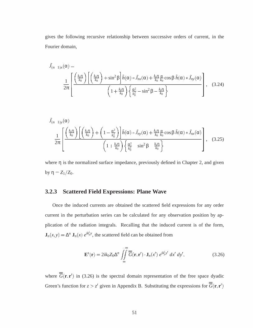
gives the following recursive relationship between successive orders of current, in the
Fourier domain,
J(n+1)x(α) =
12π
2664�
kzηk0
���kzηk0
�+sin2β
�h(α)� Jnx(α)+ kzη
k0
αk0
cosβ h(α)� Jny(α)�1+ kzη
k0
��α2
k20�sin2 β� kzη
k0
�3775 ; (3.24)
J(n+1)y(α) =
12π
2664�
kzηk0
���kzηk0
�+
�1� α2
k20
��h(α)� Jny(α)+ kzη
k0
αk0
cosβ h(α)� Jnx(α)�1+ kzη
k0
��α2
k20�sin2 β� kzη
k0
�3775 ; (3.25)
whereη is the normalized surface impedance, previously defined in Chapter 2, and given
by η = Z1=Z0.
3.2.3 Scattered Field Expressions: Plane Wave
Once the induced currents are obtained the scattered field expressions for any order
current in the perturbation series can be calculated for any observation position by ap-
plication of the radiation integrals. Recalling that the induced current is of the form,
Jn(x;y) = ∆n Jn(x) eikiyy, the scattered field can be obtained from
Es(r) = 2ik0Z0∆n
+∞ZZ
�∞
G(r ; r 0) �Jn(x0) eiki
yy0 dx0 dy0; (3.26)
where G(r ; r 0) in (3.26) is the spectral domain representation of the free space dyadic
Green’s function forz> z0 given in Appendix B. Substituting the expressions forG(r ; r 0)
51

from Appendix B into (3.26) and integrating first with respect toy0 and thenky gives
Es(r) =�k0Z0∆n
2π
+∞ZZ
�∞
1kz
ei(kxx+kiyy+kzz)fhh+ vvg �Jn(x
0)e�ikxx0dx0 dkx; (3.27)
where the unit vectors,h; v, in (3.27) are given by
h =k� zjk� zj =
kiy x�kx yqkx
2+kiy2
(3.28)
and,
v =1k0
h�k =�kxkz x�ki
ykzy+(kx2+ki
y2) z
k0
qkx
2+kiy2
: (3.29)
Noting that+∞R�∞
Jn(x0)e�ikxx0dx0, in (3.27) is simply the Fourier transform ofJn(x0) with
α = kx the final form of the scattered field for plane wave excitation is
Esn(r) =�k0Z0∆n
2π
+∞Z
�∞
1kzfhh+ vvg � Jn(kx)e
i(kxx+kiyy+kzz) dkx; (3.30)
where subscriptndefines the order of the perturbation series solution, andkz=q
k02�kx
2�kiy2.
3.2.4 Saddle Point Evaluation: Plane Wave Integral
For ρ =p
x2+z2 � λ, standard saddle point techniques can be used to evaluate the
integral in (3.30) [15, 34]. If the slowly varying function (f g� Jn(kx)) in 3.30) is non-zero in
the vicinity of the saddle or stationary point, stationary phase techniques, equivalent to first
order saddle point method, can be applied. Evaluating the exponential function,f (kix) =
kxx+ kzz, at it’s extrema gives the following expressions forkx and kz at the stationary
52

points,
kx =q
k20�ki
y2cosψ ∆ ki
ρ cosψ
kz = kiρ sinψ;
(3.31)
whereψ is the scattering angle defined from thex axis, and positive towards thezaxis, in the
x�zplane andkiρ = k0sinβ. Applying stationary phase for a one dimensional integral [35]
to (3.30) gives the following far zone scattered field expression for plane wave excitation:
Esn(r) =� k0Z0∆nq
2πkiρρfhh+ vvg � Jn(k
iρ cosψ) ei(ki
ρρ� π4) eiki
yy; (3.32)
where the unit vectors,h; v, in (3.32) are evaluated at the stationary points and are explicitly
given at these points by
h =k� zjk� zj =
�kiρ cosψ y+ki
y xqki
ρ2cos2 ψ+ki
y2
=�ki
ρ cosψ y+kiy xq
k20 cos2ψ+ki
y2sin2 ψ
; (3.33)
and,
v =1k0
h�k =�ki
ρkiysinψ y�ki
ρ2sinψcosψ x+(k2
0 cos2 ψ+kiy2sin2 ψ) z
k0
qk2
0 cos2 ψ+kiy2sin2 ψ
: (3.34)
3.3 Short Dipole Excitation
To extend the perturbation solution to include excitation by a short dipole the incident
dipole fields are represented in the form of a continuous spectrum of plane waves. The
methods of the previous section for plane wave excitation can then be applied to each spec-
tral component and the resulting expressions simply integrated over the entire dipole spec-
trum. Again stationary phase techniques (first order saddle point) can be applied to evaluate
the resulting integrals when both source and observation are distant from the transition.
53
Consider a short dipole of lengthl carrying a sinusoidal current of amplitudeI0 and
located atr0 = x0x+ y0y+ z0z. The field emitted from this dipole at some observation
point r = xx+yy+zz for z< z0 can be expressed as a continuous spectrum of plane waves
and is given by
Ei(r) =�I0lk0Z0
8π2
+∞ZZ
�∞
�1ki
z[I � K iK i
k20
] � l e�iK i �r0
�eiK i �r dki
x dkiy; (3.35)
whereK i = kixx+ ki
yy� kizz, ki
z =q
k20�ki
x2�ki
y2, and unit vectorl indicates the dipole
orientation. The integrand of (3.35) can be restated asE0 eiK i �(r�r0), where
E0 =�I0lk0Z0
8π2
1ki
z
"l � K i � l K i
k20
#: (3.36)
Recognizing that the integrand describes a plane wave propagating alongK i
k0vector and
using the linearity property of electromagnetic waves, the scattered field can be expressed
as a superposition of scattering from individual plane waves or
Esdn(r) =
+∞ZZ
�∞
X(K i) e�iK i �r0 dkix dki
y (3.37)
where the subscriptdn indicates the scattered dipole fields from the current of ordern
in the perturbation series, andX(K i) is the scattered field generated from each spectral
component of the dipole, of propagation vectorK i , and given by (3.30).
3.3.1 Stationary Phase Evaluation: Short Dipole
Again considering a situation where distance between source and observation are large
compared to wavelength, and also where both are distant from the transition in terms of
wavelength, then stationary phase techniques can be used to evaluate the integrals of (3.37).
Recognizing that the expression forX(K i) in the far-field of the impedance transition is as
54

described by (3.32) and substituting this expression into (3.37) gives the following expres-
sion for the far-zone scattered fields,
Esdn(r) =
+∞ZZ
�∞
X(K i) eikiρρ eiki
yy e�iK i �r0 dkix dki
y; (3.38)
where the exponential termseikiρρ andeiki
yy have been factored out ofX(K i). Applying
stationary phase for two dimensional integrals [36] and noting that the exponential function
is given by
f (kix;k
iy) = ki
y(y�y0)�kixx0+ki
zz0+kiρρ; (3.39)
the components ofK i at the stationary points are found to be
kix =
�x0(ρ+ρ0)
ρ0RSk0
kiy =
(y�y0)
RSk0
kiz =
z0(ρ+ρ0)
ρ0RSk0;
(3.40)
whereρ0 =q
x20+z2
0 andRS=p
(y�y0)2+(ρ+ρ0)2. Evaluating (3.38) at the stationary
points gives the final form of the scattered electric field for source and observation distant
from each other and the transition, or
Esdn(r) = X(K i)
2πiC
eik0RS; (3.41)
55

where againK i is evaluated at the stationary points. and where
C=
vuut ∂2 f
∂kix2
∂2 f
∂kiy2 �
�∂2 f
∂kix∂ki
y
�2
: (3.42)
Explicit expressions for (3.42) are obtained by evaluating the second derivatives of the
exponential function at the stationary point and the resulting expressions are given by,
∂2 f
∂kix2 =� ρ2
0
z0 kiz; (3.43)
∂2 f
∂kiy2 =�ki
z2+ki
y2
kiz3 z0� k2
0
[k20�ki
y2]3=2
ρ; (3.44)
∂2 f∂ki
x∂kiy=�ki
xkiy
kiz3 z0: (3.45)
Simplified expressions forJn(kx), wherekx = kiρ cosψ = k0sinβcosψ, can be derived by
evaluating (3.24) and (3.25) at the stationary points withE0x andE0y in (3.24) and (3.25)
defined by (3.36) Recognizing that sinβ = (ρ+ρ0)RS
, cosβ = y�y0RS
; andkz = k0sinβ sinψ the
following expression for the induced surface currents in the Fourier domain are obtained.
J(n+1)x(α) =
� 12π
ηsinβ�[ηsinψ+sinβ] h(α)� Jnx(α)+cosψ cosβ h(α)� Jny(α)
(1+ηsinβ sinψ)(η+sinβ sinψ)
; (3.46)
56

J(n+1)y(α) =
� 12π
�
ηsinβ sinψ+1�sin2β cos2ψ�h(α)� Jny(α)+sinβ cosβ cosψh(α)� Jnx(α)
(1+ηsinβ sinψ)(η+sinβ sinψ)
:
(3.47)
3.3.2 Near-field Observation
For certain cases it is desirable to allow the observation position to move into the near-
field of the impedance transition while keeping the source distant, therefore allowing the
spectral domain integration overkix;k
iy in (3.37) to still be performed in an approximate
fashion using stationary phase techniques, while the scattered field for a given spectral
component,X(K i) in (3.37) is evaluated numerically. In order to evaluate the integration
overkix;k
iy by applying stationary phase techniques, it is necessary to have an explicit ex-
pression for the phase function, or high frequency component of the integrand. As the
Fourier transform of the current function is slowly varying, this high frequency component
is obviously the exponential factor in the integral expression forX(K i) given in (3.30).
Analysis shows however, that there is no analytic solution for the stationary points of the
dipole fields when the integrand is in this form. An alternate mapping in the complex plane
can be applied however as the contour is no longer along the real axis,kiy is complex and
the integration overy0 in (3.26) is no longer straightforward. If however we subtract the
stationary points of the integrand in (3.30) (and given in (3.31)) from the exponential factor
of (3.30) and add them back, the following expression is obtained
Es(r) =�k0Z0∆n
2π
+∞Z
�∞
1kzfhh+ vvg � Jn(kx)e
i((kx�kiρ cosψ)x++(kz�ki
ρ sinψ)z) dkx ei(kiρρ+ki
yy);
(3.48)
wherex= ρcosψ, y= ρsinψ, and therefore thatkiρ(cosψ x+sinψ y) = ki
ρρ. Recognizing
that the exponential function inside the integrand of (3.48) transitions to zero as the ob-
57

servation moves into the far-field, it is obvious that this function is slowly varying for all
observation positions and that the rapidly varying component,kiρρ has been factored out of
the integrand. The integrand of (3.48) can now be evaluated numerically, while the high
frequency phase factor is of the form given in (3.38) and can be evaluated asymptotically,
in a similar fashion.
3.3.3 Error Bound
An important feature of the perturbation solution is its convergence properties and it is
appropriate at this point to establish some sense of these properties, i.e., for what values
of ∆ the perturbation expansion of (3.15) converges to the exact solution. To characterize
the limits of the perturbation method an error bound is determined on the maximum∆ al-
lowable, for a given incidence angle, and for a particular impedance profile. Analysis of an
error bound for the case of plane wave incidence will also give a sense of the convergence
of the perturbation series for dipole excitation in cases where one spectral component of the
dipole radiation is the dominate excitation. Mathematically this can be shown by finding
the radius of convergence of the expanded current series, in terms of the perturbation pa-
rameter∆. Even for a value of∆ > 1 the series will converge if the current coefficients are
decreasing for higher orders. Let us first consider a limiting case for which an exact solu-
tion exists. This corresponds to a constant perturbation function (h(x) = 1) whose Fourier
transform is aδ function. Applying this to (3.18) and (3.19), and assumingβ = π=2, gives
the following forms for the horizontally and vertically polarized currents:
J0h(x) =[sinφi x+cosφi y]
12Z1(1+∆)+ Z0
2cosθi
eik0 sinθi(cosφix+sinφiy); (3.49)
J0v(x) = [cosφi x+sinφi y]cosθi
12Z1(1+∆)+ Z0cosθ
2
eik0 sinθi(cosφix+sinφiy); (3.50)
58
After some algebraic manipulations these equations can be put in the form of
J0 h;v(x) = K1υ� 1
1+ ∆υ; (3.51)
whereK is some constant parameter and
υ =
8>><>>:
1ηcosθi +1 for J0h(x);
cosθi
η +1 for J0v(x):
(3.52)
The Taylor Series expansion of (3.51) will converge uniformly for all∆ < υ, which indi-
cates that the radius of convergence for low impedance surfaces can be very high.
3.4 Validation & Results: Perturbation Technique
In this section analytic results based on the perturbation solution are validated and are
compared with those obtained from independent techniques where possible. The impedance
values of the soil are again derived from the values of permittivity and conductivity given
by Hipp [1] for San Antonio Gray Loam with a density of 1:4 g=cm3 and shown in Ta-
ble 1.1, with the impedance values of the water derived from the equations for complex
permittivity given by Ulaby,et al. [5], as previously stated. Once the impedance values
for the soil and water are determined, the perturbation parameter∆ can be calculated from
(3.13).
To validate the perturbation method the case of plane wave excitation is first examined.
Results are generated for the case of scattering from an abrupt impedance discontinuity or
impedance step insert, which is representative of a river. Effects of varying the perturbation
parameter∆ (equivalent to varying soil moisture) are investigated and compared to a GTD
solution. Scattering for oblique incidence angles is also analyzed, as well as the effect of
varying the insert width. A comparison is made between the scattered fields from an abrupt
59

discontinuity (insert) to those from a more gradual transition, which can better represent an
actual land/water transition. As previously mentioned the effect of a land/sea transition on
the total fields of an infinitesimal dipole is then examined.
Note that Figure 3.1, shown previously, describes the scattering coordinates for both
types of excitation.
3.4.1 Plane Wave Excitation
In this section results will be shown and discussed for plane wave excitation of the
impedance surface. As mentioned, the the impedance transition will initially be mod-
eled as an abrupt discontinuity, or impedance step insert. The step insert will be used
to validate and characterize the method by comparing with a GTD solution, normal in-
cidence (β = π=2). Results will then be shown for various oblique incidence angles. A
more gradual impedance transition function, which better represents an actual riverbed,
will then be described and results compared with that of the step insert. Also the effect
of varying the insert width will be discussed. Note that all results for plane wave excita-
tion, show the normalized scattering width,σs=λ, around the specular scattering cone, with
σs = 2πρ(jEsj=jEij) asρ! ∞.
As a validation of the proposed technique, it is important to know for what values of∆
a first order solution will give desirable accuracy. With this in mind results were generated
for first and second order scattered fields using the perturbation method and compared to
a third order GTD solution for the step impedance function, for the 2-D case of excitation
across the insert (φi = 180Æ). The order of the GTD solution describes to what degree
diffracted fields are accounted for, i.e., first order are the diffracted fields generated by the
incident wave, second order are the diffracted fields generated by these initial diffracted
fields interacting with the diffracting edges, etc. All results shown for plane wave excita-
tion are for a step insert 5λ wide, excited at 30MHz and normal incidence (β = π=2). The
insert is assumed to have a normalized complex impedance of 0:0369� i0:0308, represen-
60

tative of saline water, with a salt content of 4pp=1000, and results are shown for varying
soil moistures (gravimetric moisture content). Figures 3.2 and 3.3 show results from the
first and second order perturbation solution, compared to the mentioned GTD solution,
for TE and TM cases, respectively (TE, TM, transverse electric and magnetic toz) and
for gravimetric soil moistures of 20, 10, and 5%, equivalent to normalized impedanceη of
0:12� i0:07; 0:15� i0:09; 0:3� i0:1, andj∆j= 0:6529; 0:7263; 0:8594, respectively, with
incidence angleθi at 45Æ. As soil moisture is varied from 20% to 5% the first and second
0 20 40 60 80 100 120 140 160 180−80
−60
−40
−20
0
20
ψ (Degrees)
Sca
tterin
g W
idth
, σ2D
/λ (
dB)
(a) Moisture Content = 20%,j∆j= 0:6529
0 20 40 60 80 100 120 140 160 180−80
−60
−40
−20
0
20
ψ (Degrees)
Sca
tterin
g W
idth
, σ2D
/λ (
dB)
(b) Moisture Content = 10%,j∆j= 0:7263
0 20 40 60 80 100 120 140 160 180−80
−60
−40
−20
0
20
ψ (Degrees)
Sca
tterin
g W
idth
, σ2D
/λ (
dB)
(c) Moisture Content = 5%,j∆j= 0:8594
Figure 3.2: TE case, normalized bistatic echo width (σs=λ) of an impedance step insert, 5λwide, equivalent to slightly saline water (4pp=1000 salt content,η = 0:0369�i0:0308). θi = 45Æ, φi = 180Æ, first (- - - - - ) and second order (� � � � �)perturbation technique compared with GTD (———) for varying soil moisture.
61

order perturbation solutions begin to degrade in accuracy. The degradation is especially
significant for the TM case and near grazing observation.
The convergence property of the perturbation solution as a function of the width of the
insert step function was also observed. The insert width was varied from 1 to 20λ with the
accuracy of both the TM and TE results essentially insensitive to insert width variations.
0 20 40 60 80 100 120 140 160 180−80
−60
−40
−20
0
20
ψ (Degrees)
Sca
tterin
g W
idth
, σ2D
/λ (
dB)
(a) Moisture Content = 20%,j∆j= 0:6529
0 20 40 60 80 100 120 140 160 180−80
−60
−40
−20
0
20
ψ (Degrees)
Sca
tterin
g W
idth
, σ2D
/λ (
dB)
(b) Moisture Content = 10%,j∆j= 0:7263
0 20 40 60 80 100 120 140 160 180−80
−60
−40
−20
0
20
ψ (Degrees)
Sca
tterin
g W
idth
, σ2D
/λ (
dB)
(c) Moisture Content = 5%,j∆j= 0:8594
Figure 3.3: TM case, normalized bistatic echo width (σs=λ) of an impedance step insert, 5λwide, equivalent to slightly saline water (4pp=1000 salt content,η = 0:0369�i0:0308). θi = 45Æ, φi = 180Æ, first (- - - - -) and second order (� � � � �)perturbation technique compared with GTD (———) for varying soil moisture.
The effect of oblique incidence on the scattered wave was also examined for the case
of the impedance step insert when excited by a plane wave. First order perturbation re-
62

sults were generated with the insert again representative of slightly saline water and the
surrounding impedance representative of the same San Antonio gray loam, with a mois-
ture content of 10%. Figure 3.4 shows the bistatic scattering width for co-polarization
results, with 3.4a showing the TE case and 3.4b the TM case. Figure 3.5 shows the cross-
polarization results for oblique incidence. Againθi = 45Æ, with φi rotated at the oblique
angles, 180Æ;135Æ, and 90Æ. Referring to Figure 3.4a and Figure 3.4b, the peak scattering
0 20 40 60 80 100 120 140 160 180−70
−60
−50
−40
−30
−20
−10
0
10
ψ (Degrees)
Sca
tterin
g W
idth
, σs /λ
(dB
)
(a) TE case,φi= 180 (———), 135 (- - - - -),
and 90Æ (� � � � �).
0 20 40 60 80 100 120 140 160 180−70
−60
−50
−40
−30
−20
−10
0
10
ψ (Degrees)
Sca
tterin
g W
idth
, σs /λ
(dB
)
(b) TM case,φi=180 (——— ), 135 (- - - - -),
and 90Æ (� � � � �).
Figure 3.4: Normalized bistatic echo width, (σs=λ), of an impedance step insert of width5λ, equivalent to slightly saline water (4pp=1000 salt content,η = 0:0369�i0:0308). Surrounding soil has a gravimetric moisture contend of 10% (j∆j =0:7263). Incidence is atθi = 45Æ, first order perturbation technique.
63

for, φi = 180Æ, is shown to be at approximately the specular angle ofψ = 45Æ. At φi = 90Æ
the incident wave is along the step insert and the scattering pattern is symmetric in thex�z
plane as expected.
Theoretically no cross-polarization results can exist for an incidence angle ofφi = 180.
As φi is rotated towards 90Æ cross-polarization levels become more significant. Figure 3.5
shows cross-polarization results, again in terms of normalized scattering width, for plane
wave excitation withθi = 45Æ andφi = 90Æ. Note that as the incident field is rotated to
a position along the step insert,φi = 90Æ, the cross-polarization levels rise and in fact the
cross-polarization forTETM with φi = 90Æ is the highest level for all results including co-
polarization curves. This indicates that receiver polarization (measuring the scattered field)
need be adjusted, for optimum polarization matching, as the incident field propagation
vector moves about the step insert.
0 20 40 60 80 100 120 140 160 180−70
−60
−50
−40
−30
−20
−10
0
10
20
ψ (Degrees)
Sca
tterin
g W
idth
, σs /λ
(dB
)
Figure 3.5: Normalized bistatic echo width, (σs=λ), of an impedance step insert of width5λ, equivalent to slightly saline water (4pp=1000 salt content,η = 0:0369�i0:0308). Surrounding soil has a gravimetric moisture contend of 10% (j∆j =0:7263). Incidence is atθi = 45Æ, φi = 90Æ, first order perturbation technique.TETM (——–), TMTE (- - - - -).
In order to more accurately represent an actual riverbed an impedance function with a
more gradual transition than the step function was generated and results compared to those
generated by the step insert at normal incidence. The transition is made over a distance of
λ=2 and and the width of the gradual impedance function set at 5λ, the same as the step
64

insert. The width of the gradual impedance function is defined as the distance between
points where the function is 3 dB below maximum. Again first order perturbation results
are shown with the transition representative of slightly saline water and the surrounding
soil having a moisture content of 10%. The results for the step insert, shown previously
with φi = 180Æ are overlayed with those of the gradual impedance transition and are seen in
Figure 3.6a and Figure 3.6b for TE and TM polarizations, respectively. As can be seen in
0 20 40 60 80 100 120 140 160 180−70
−60
−50
−40
−30
−20
−10
0
10
ψ (Degrees)
Sca
tterin
g W
idth
, σs /λ
(dB
)
(a) TE case
0 20 40 60 80 100 120 140 160 180−70
−60
−50
−40
−30
−20
−10
0
10
ψ (Degrees)
Sca
tterin
g W
idth
, σs /λ
(dB
)
(b) TM case
Figure 3.6: Normalized bistatic echo width, (σs=λ), of an impedance step insert of width5λ, equivalent to slightly saline water (4pp=1000 salt content,η = 0:0369�i0:0308). Surrounding soil has a gravimetric moisture contend of 10% (j∆j =0:7263). Incidence is atθi = 45Æ, φi = 180Æ, first order perturbation technique.Step insert (——–) compared to gradual transition (-- - - -).
65

these figures, the gradual impedance transition tends to lower and pull the side lobe levels
towards the specular scattering direction ofψ = 135Æ. This is as expected since a more
gradual transition disturbs the induced surface currents less and in the limit should reduce
to case of specular scattering only.
3.4.2 Dipole Excitation: Land/Sea Interface
In this section the effect on the total fields of an infinitesimal dipole by an impedance
transition will be analyzed. For the case of an impedance step insert, examined in the
previous section, the effects of the transition are highly localized to the immediate vicinity
of the transition and has little effect on the total dipole fields away from the transition,
i.e., the effects of the homogeneous surface dominate here. Instead the case of a seashore,
or land/sea transition, which can have a significant effect on the total dipole fields distant
from the transition, will be examined. For all results presented in this section the impedance
of the land or ground, defined asZg will be the usual San Antonio gray loam, with 10%
gravimetric moisture content, and equivalent normalized impedanceηg, of 0:15� i0:09,
while the impedance of the water or sea, defined asZw will have a salt content of 4pp=1000
and normalized impedanceηw = 0:0369� i0:0308, as previously described. In this section
all field quantities shown are defined in terms of path loss, where path loss is the field
quantity normalized to the magnitude of the incident dipole field,E=jEi j.To analyze the land/sea transition we will begin with the case of an abrupt transition
and then modify the resulting expressions to include the case of a more gradual transition.
Referring to Figure 3.7, the impedance transition function for an abrupt land/sea transition
can be represented by a signum (sgn(x)) function with an offset, where thesgn(x) function
66

is defined as,
sgn(x) =
8>><>>:�1
2 for x< 0
12 for x> 0;
(3.53)
Due to the offset of the impedance transition function in the spatial domain, its Fourier
Earth Water
ReflectionBoundary
Zg
Zw
Eiθ i θ i
Transition Width
0.9 Zw
0.9 Zg Z g Zw+
2
Figure 3.7: Geometry of a Land/Sea Interface
transform contains aδ function, and the perturbation technique described cannot be imme-
diately applied. In order to apply the perturbation technique the impedance transition will
be dealt with in a mean sense, i.e., we assume that the unperturbed impedanceZ1, in (3.13),
is the mean value of the impedance transition function or
Z1 =Zg+Zw
2; (3.54)
67

as seen in Figure 3.7. The assumption of a mean impedance as the unperturbed impedance
is a valid assumption in terms of the first order and higher fields in the perturbation se-
ries. For source and observation near the impedance surface and distant from both each
other and the transition the assumption of a mean impedance for the homogeneous surface
should also produce the appropriate zeroth order (diffracted) fields. For this situation, the
observation is in the immediate vicinity of the Geometrical Optics (GO) reflection bound-
ary (boundary between GO fields reflected from land and GO fields reflected from the sea,
see Figure 3.7) and as in this region higher order terms in the asymptotic expansion of the
diffracted fields are dominate (Norton surface wave), there is no sharp transition at the re-
flection boundary between the fields diffracted from the land and those diffracted from the
sea (GO component of the diffracted field is not dominate), and thus the assumption of a
mean impedance for the homogeneous surface is valid. As observation and or source are
moved away from the impedance surface the dominate component of the diffracted fields
is the specular component, and the reflection boundary becomes more sharply defined.
In this region the mean impedance assumption, is invalid and the perturbation solution
will not produce the correct diffracted fields. For this case however, the space wave (di-
rect+diffracted) is the dominate contributor to the total fields and the diffracted fields can
be recovered by simply assuming a sharp reflection boundary and calculating the diffracted
fields from land or sea respectively, on either side of this boundary.
The impedance transition function,h(x), can now be written directly as,
h(x) =�sgn(x); (3.55)
h(α) =iα; (3.56)
in the spatial and Fourier domain, respectively. To find the appropriate∆, (3.54) and (3.55)
68
are substituted into (3.13). Solving for∆ gives,
∆ =Zg�Zw
Z1: (3.57)
In order to represent a more gradual transition function, (3.55) is modified to,
h(x) =�sgn(x)(1�e�κjxj); (3.58)
which in the Fourier domain becomes,
h(α) =iα� iα
α2+κ2 : (3.59)
In (3.58)κ is a constant parameter, whereκ!∞ as the width of the transition goes to zero,
i.e., an abrupt transition.
Before beginning analysis of the land/sea transition it is appropriate to note the intro-
duction of a simple pole in the impedance transition function of (3.56), and therefore in
the scattered field integral of (3.30). This pole occurs at the reflection boundary of the
GO fields and while it can be shown this is a non-contributing pole care must be taken
when evaluating the integral of (3.30) asymptotically. As the stationary point approaches
the pole (observation approaches the reflection boundary) the effect of the stationary point
cannot be separated from the effect of the pole and modified asymptotic approaches must
be employed. In the literature two approaches are discussed, the additive, and multiplica-
tive method [37, 15]. In the additive method the integrand is regularized by subtracting
and adding an appropriate factor and the resulting expression expanded in an asymptotic
fashion. In the multiplicative method the integrand is regularized, appropriately by a multi-
plicative factor and also expanded into an asymptotic series. While both expansions can be
shown to be equivalent, the equivalence holds only for the complete asymptotic series of
both expansions [38]. When the series are truncated the equivalence does not hold and the
69
truncated series may produce different results. In the analysis of the land/sea problem only
the first order term in the asymptotic series is retained and it was observed that the mul-
tiplicative method produced proper results, while the additive method did not sufficiently
compensate for the immediate presence of the pole, thus implying that higher order terms
in the asymptotic expansion are required to utilize this method.
To begin analysis of the land/sea transition we first examine the effect of a gradual tran-
sition on the scattered fields. A vertical electric dipole, operating at 30MHz, is placed 100λ
from the impedance transition, along the negativex axis and 100λ above the impedance
surface (x0 = �100λ;y0 = 0;z0 = 100λ). Observation is across the transition (y = 0) at
a fixed radial distance of 50λ. Note that for all results in this section thez component of
the scattered field is shown. For source and observation near the impedance surface the
z scattered field component from a vertical electric dipole is the dominate scattered field
component for any dipole orientation, and thus is of most interest in this analysis. Fig-
ure 3.8 shows the path loss for transition widths of 0 (abrupt transition), 1, and 10λ, where
the transition width is defined as the distance between the points where the transition func-
tion is 0:9 that ofZg or Zw, over land or sea, respectively (see Figure 3.7). As can be seen
in Figure 3.8, the effect of widening the transition is to focus the scattered energy in the
specular direction (ψ0 = 135Æ, note thatψ0 = (π�ψ) in the figures shown,φi = 0). How-
ever, in the neighborhood of the specular direction the transition width has little effect on
the field levels. This is a significant observation as it indicates that for source and obser-
vation near the surface, and again distant from each other and the transition, the width of
the transition will have negligible effect on the scattered fields as in this region the specular
angle is pushed to near-grazing observation, i.e., observation is always near the specular
point. This makes intuitive sense also as the width of the transition is less apparent as it
approaches the horizon of an observer.
In Figure 3.9 a similar problem is analyzed but for this case the transition width is fixed
at 1λ and the radial observation distanceρ is varied from 50 to 10 to 1λ. As can be seen in
70

0 50 100 150−80
−70
−60
−50
−40
−30
−20
ψ′ (Degrees)
|Ezs |/|
Ezi |
Figure 3.8: Magnitude (dB), Path loss, land/sea transition located atx = 0, z componentof the scattered fields for a vertical (z-directed) electric dipole. Observationρis fixed at 50λ, observationy = 0, for dipole position ofx0 = �100λ;y0 =0;z0 = 100λ. Ground moisture is 10% (ηg = 0:15� i0:09), Sea is salinewater (4pp=1000 salt content,ηw = 0:0369� i0:0308, j∆j = 1:14). Resultsfor transition widths of 0 (———), 1 (- - - - - ), and 10λ (� � � � �). Notethatψ0 = π�ψ in curves.
Figure 3.9 this has the effect of spreading the energy out, around the specular direction. The
is indicative of the fact that for far-field observation the induced surface currents around the
transition look like a line source, while as observation is moved from far-field to near-field
the current distribution begins to look more like a distributed source.
In Figure 3.10 the transition width is fixed at 1λ, observation is fixed at a radial distance
of 100λ, with the three curves reflecting an offset of 0, 50, and 100λ in the y dimension
(oblique incidence). As can be seen in Figure 3.10 the effect of the obliquity across the
transition is to increase the amount of energy in the backscatter direction. This again makes
intuitive sense as the energy from the incident wave is coupled into a component along the
transition.
As a final analysis of the effects of a land/sea transition on the fields of an infinites-
imal dipole, we place a vertical electric dipole atx0 = �100λ;y0 = 0, move the source
and observation heights to 1, 5, and 10λ (for these examples source and observation are at
same height above surface), and compare the path loss of the space wave to that of the total
71

0 50 100 150−80
−70
−60
−50
−40
−30
−20
−10
ψ′ (Degrees)
|Ezs |/|
Ezi |
Figure 3.9: Magnitude (dB), Path loss, land/sea transition, located atx= 0, zcomponent ofthe scattered fields for a vertical (z-directed) electric dipole. Transition widthis fixed at 1λ, observationy = 0, for dipole position ofx0 = �100λ;y0 =0;z0 = 100λ. Ground moisture is 10% (ηg = 0:15� i0:09), Sea is saline water(4pp=1000 salt content,ηw = 0:0369� i0:0308,j∆j= 1:14). Results for radialobservation distanceρ of 50λ (———), 10λ (- - - - - ), and 1λ (� � � � �).Note thatψ0 = π�ψ in curves.
fields. Observation is on a radial line between source and observation, fromx = �50λ to
x = 150λ. Note that other parameters are the same as for previous results in this section,
with the transition width at zero (abrupt transition). The results are seen in Figure 3.11, with
Figure 3.11a, b, and c, comparing the space wave (direct+diffracted) to the total fields (in-
cluding the effects of the transition) and showing the results for source/observation heights
of 1, 5, and 10λ, respectively. As mentioned for this case of source and observation near
the impedance surface the Norton surface wave, which decays at a rate of 1=R2, is the dom-
inate component of the diffracted fields. Noting that the scattered fields also decay at this
rate it is expected that the effect of the land/sea interface will have a significant effect on
the total dipole fields and as is seen in these figures, the effect of the land/sea transition on
the total fields is significant even at distances far from the transition. An additional note
on the plots in Figure 3.11. An abrupt discontinuity is observed at the reflection boundary
(x= 100λ), where the diffracted fields transition from ground reflections to reflections from
the sea. Normally it would be expected that the addition of the scattered fields to the total
72

0 50 100 150−80
−70
−60
−50
−40
−30
−20
−10
ψ′ (Degrees)
|Ezs |/|
Ezi |
Figure 3.10: Magnitude (dB), Path loss, land/sea transition, located atx= 0, z componentof the scattered fields for a vertical (z-directed) electric dipole. Transitionwidth is fixed at 1λ, Radial observationρ is fixed at 10λ, for varyingy offsetbetween source and observation (oblique incidence), and for dipole positionof x0 =�100λ;z0 = 100λ. Ground moisture is 10% (ηg = 0:15� i0:09), Seais saline water (4pp=1000 salt content,ηw = 0:0369� i0:0308,j∆j = 1:14).Results for offset iny of 0 (———), 50 (- - - - - ), and 100λ (� � � � �).Note thatψ0 = π�ψ in curves.
fields should produce uniform results across the reflection boundary, i.e., a smooth transi-
tion between the fields diffracted from land and those diffracted from water. The abrupt
transition observed in these results can be explained by observing the transition function
seen in Figure 3.7 and its Fourier transform. The transition function is infinite in extent,
and as it is assumed that only one spectral component of the dipole fields excites the tran-
sition uniformly across the entire extent of the impedance surface, the transition function
contains infinite energy. Thus while its Fourier transform exists, it is not finite in energy,
at the reflection boundary. To show this we weight the transition function of (3.55) with a
dampening factor, or
h(x) =�sgn(x)e�κjxj (3.60)
73

whose Fourier transform is given by,
h(α) =iα
α2+κ2 ; (3.61)
The scattered fields produced by this transition function are compared to those from the
original abrupt transition, for source and observation heights of 1λ, and the results are
shown in Figure 3.12. As expected the effect of a dampened transition, with finite energy
smoothes the transition in the scattered fields over the reflection boundary. While this
result explains the apparent discontinuity in the fields across the reflection boundary it is
not apparent that this modification will produce acceptable results. Questions arise as to the
appropriate dampening factor to produce physical results. A more appropriate adjustment
may be made to the direct dipole fields. In implementing the perturbation technique it
is assumed that the dipole source is distant from the transition and that only one spectral
component excites the transition. While this is a valid assumption it assumes that one plane
wave illuminates the entire impedance surface (infinite energy across the surface), and does
not account for the pattern and decay of the dipole fields away from the transition. A more
proper solution may be to expand the dipole fields in a way which accounts for the dipole
field pattern across the impedance surface. In any case while the abrupt discontinuity across
the reflection boundary observed in Figure 3.11 is not in fact physical, the fields on either
side of the boundary are proper.
Finally, for the same test case the dipole is placed 1λ above the impedance surface and
path loss is observed in a rectangular grid, 1λ above the surface. Note that the transition is
located atx= 0 in these figures (abrupt transition). Figures 3.13 shows the path loss, with
Figures 3.13a showing the space wave and Figures 3.13b showing the total fields. As can
be seen in comparing the field plots, the land/sea transition has a significant effect on the
total dipole fields.
74

3.5 Chapter Summary: Impedance Transition
In this chapter the model for scattering and diffraction from an impedance half-space,
representing a locally flat, lossy Earth was extended to include an impedance transition
such as caused by a river or land/sea interface. Using the field equivalence principle, the
problem is formulated in terms of an integral equation for a fictitious electric current in-
duced on the variable impedance surface. A perturbation technique was used to derive
a recursive solution for any order surface currents in the perturbation series, in terms of
the previous order. An error bound was established to give some sense of the radius of
convergence of the perturbation series. Stationary phase techniques were used to evaluate
far-field expressions for both plane wave and short dipole excitations. Initial results were
shown for plane wave excitation to characterize and validate the perturbation technique.
Examining the case of an impedance step insert, results from the perturbation model, for
the 2-D case were compared to those of a GTD solution. It was shown that for impedances
representative of a river surrounded by moist soil, that the first order perturbation results
produced acceptable accuracy when the soil moisture content was at or above 10%. Even
for soil moisture levels below 10% the first order perturbation results were acceptable for
TE incidence with TM showing a degradation at near-grazing observation angles of 5 or
6 dB. It was observed that, for oblique incidence angles, the cross-polarization levels for a
TM polarized field, incident along the river, dominated the scattering levels. Effects of a
more realistic, gradual impedance transition were also examined. The effects on the total
fields of an infinitesimal electric dipole by a land/sea transition were then examined. Not-
ing that the ˆz component of the received electric fields from a vertical dipole are dominate
for source and observation near the impedance surface this case was examined. To imple-
ment the transition in the Fourier domain the impedance transition was dealt with in a mean
sense, which is an acceptable approximation for source and observation near the impedance
surface. Results from an abrupt transition were generated and compared to those from a
more gradual transition. It was shown that the while a more gradual transition tends to fo-
75

cus the scattered field energy in the specular direction, the field levels in the neighborhood
around specular scattering was essentially unaffected, thus indicating that for source and
observation near the impedance surface the effects of the transition width are negligible.
Observation of the path loss in the total fields when compared with the path loss of the
space wave (direct+diffracted) showed that the land/sea transition has a significant effect
on the total dipole fields, even distant from the seashore.
Having developed a complete model in the last two chapters to account for the effects
of an impedance half-space, which can contain a general one-dimensional impedance vari-
ation, on the propagating radio wave, it is now desired to include the effects of natural
obstacles on the propagating wave. With this in mind, in the next two chapters a diffraction
model is developed which accounts for the effects on propagation of mountains, hills, or
ridgelines, which can be modeled as single curved, convex surface. For obstacles with a
large local radius of curvature, diffraction effects can be modeled locally by a right circular
cylinder. In the next chapter a somewhat novel model to predict scattering and diffraction
from right circular cylinders, when excited by a plane wave at oblique angles is developed.
In the chapter that follows the model is extended to include scattering and diffraction from
a general, singly curved, convex surfaces.
76

−50 0 50 100 150−30
−25
−20
−15
−10
−5
0
5
10
x (Wavelengths)
|Ez|/|
Ezi |
(a)z0 = z= 1λ
−50 0 50 100 150−30
−25
−20
−15
−10
−5
0
5
10
x (Wavelengths)
|Ez|/|
Ezi |
(b) z0= z= 5λ
−50 0 50 100 150−30
−25
−20
−15
−10
−5
0
5
10
x (Wavelengths)
|Ez|/|
Ezi |
(c) z0= z= 10λ
Figure 3.11: Magnitude (dB), Path loss, land/sea transition, located atx= 0, z componentof the scattered fields for a vertical (z-directed) electric dipole. Transitionwidth is 0λ (abrupt), observationy = 0, observationx from �50λ to 150λ.Dipole position is atx0 = �100λ;y0 = 0λ. for varying source/observationheights. Ground moisture is 10% (ηg = 0:15� i0:09), Sea is saline water(4pp=1000 salt content,ηw = 0:0369� i0:0308,j∆j= 1:14). Results for spacewave (———), and total dipole fields (- - - - - ).
77

−50 0 50 100 150−30
−25
−20
−15
−10
−5
0
5
10
x (Wavelengths)
|Ez|/|
Ezi |
Figure 3.12: Magnitude (dB), Path loss, land/sea transition, located atx= 0, z componentof the scattered fields for a vertical (z-directed) electric dipole. Transitionwidth is 0λ (abrupt), observationy = 0, observationx from �50λ to 150λ.Dipole position is atx0 = �100λ;y0 = 0λ. Source/observation heightz0 =z = 1λ. Ground moisture is 10% (ηg = 0:15� i0:09), Sea is saline water(4pp=1000 salt content,ηw = 0:0369� i0:0308,j∆j= 1:14). Results for spacewave (———), total dipole fields, infinite transition function (- - - - - ), totaldipole fields, weighted transition function (� � � � �).
78
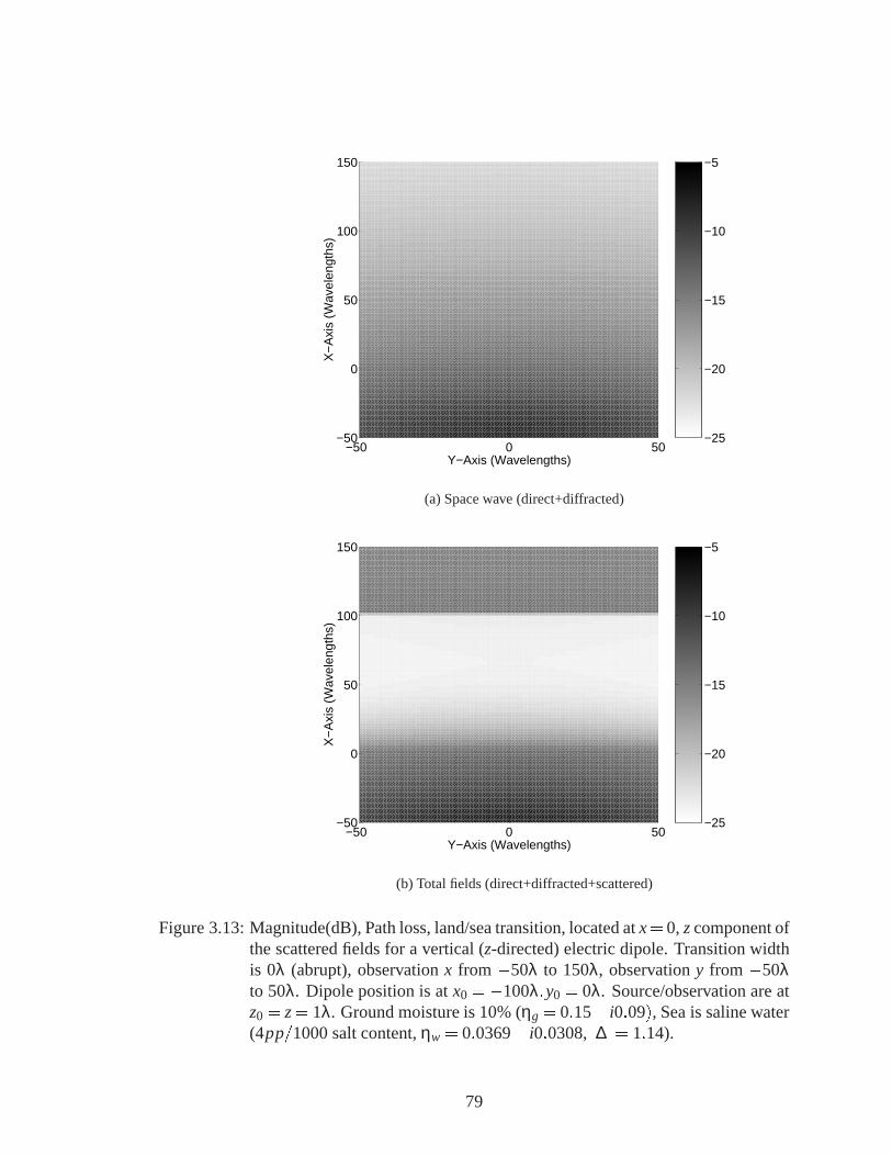
−25
−20
−15
−10
−5
−50 0 50−50
0
50
100
150
Y−Axis (Wavelengths)
X−
Axi
s (W
avel
engt
hs)
(a) Space wave (direct+diffracted)
−25
−20
−15
−10
−5
−50 0 50−50
0
50
100
150
Y−Axis (Wavelengths)
X−
Axi
s (W
avel
engt
hs)
(b) Total fields (direct+diffracted+scattered)
Figure 3.13: Magnitude(dB), Path loss, land/sea transition, located atx= 0,zcomponent ofthe scattered fields for a vertical (z-directed) electric dipole. Transition widthis 0λ (abrupt), observationx from �50λ to 150λ, observationy from �50λto 50λ. Dipole position is atx0 = �100λ;y0 = 0λ. Source/observation are atz0 = z= 1λ. Ground moisture is 10% (ηg = 0:15� i0:09), Sea is saline water(4pp=1000 salt content,ηw = 0:0369� i0:0308,j∆j= 1:14).
79

CHAPTER 4
Diffraction from Convex Surfaces: Right Circular
Cylinders
In a rural or semi-rural propagation environment, natural obstacles such as hills, moun-
tains, or ridgelines can have a significant effect on the propagating radio wave. Many
natural terrain features exhibit both curved and doubly curved surfaces. Ridge lines in
mountainous areas exhibit the features of a long curved cylinder which is essentially in-
finite in one dimension at high-frequencies. These lines may be the result of the natural
formation of the mountain chain or a feature of erosion. Geologically recent mountain
chains, while exhibiting sharp edged features, still have electrically large radii of curvature
even at HF bands. This indicates that the radius of curvature must be accounted for, and
that diffraction from curved surfaces, as opposed to knife edge diffraction, is the appropri-
ate prediction tool.
Because of the numerical complexity associated with high frequency methods for con-
vex surfaces, simpler approaches are taken which do not account for the radius of curva-
ture of the diffracting obstacle. One of the most commonly used methods of prediction is
knife-edge or Kirchhoff diffraction. This method is an application of Huygens principle in
which the diffracting obstacle is replaced by an impenetrable screen and the field distribu-
tion in the plane of the screen (aperture) is integrated to produce the fields at the desired
80

observation point. These integrals are usually in the form of either Fresnel type integrals
(intermediate range) or Fourier transforms (far-field observation). This method is simple
to implement, and for very narrow hills (small radius of curvature at the shadow bound-
ary) produces acceptable results in the far-field, away from the transition region (transition
between light and shadow), however it does not produce acceptable results for near-field
observation or in the shadow or transition regions. The method also does not account for
polarization effects, nor the shape of the obstacle (does not account for reflections from the
obstacle), and it is a 2-D method and therefore does not account for the effects of oblique in-
cidence. Luebbers [39] modeled diffracting obstacles as an impedance wedge and showed
a significant improvement over knife-edge techniques. The method is somewhat simple
to implement and is extendible to the oblique incidence case, however the accuracy of the
method is based on the assumption that the local radius of curvature at the shadow bound-
ary is less than 1=100 of a wavelength (rc� λ=100), which as mentioned tends not to occur
in nature. In addition the wedge is not a suitable representation for many natural features.
These features have a radius of curvature which makes a more gradual transition away from
the shadow boundary and creeping wave effects, which the wedge shape does not predict,
must be accounted for. For these obstacles, with a more gradual transition in radius near
the shadow boundary, wedge diffraction will not produce accurate results in the near-field
of the obstacle, especially in the deep shadow region.
With this as a motivation, in the next two chapters a somewhat novel method for the
prediction of diffraction and scattering from singly curved convex surfaces, with large,
slowly varying radii of curvature is developed. To avoid the aforementioned numerical
complexities associated with high-frequency techniques for convex surfaces, a much sim-
pler method is developed, which retains a high degree of accuracy, while avoiding the
numerical integration inherent in the existing techniques. The proposed method calculates
induced surface currents and thus through the radiation integrals gives accurate fields in
all regions around the surface. The induced surface currents on a general convex surface,
81

again of large, slowly varying radius of curvature, can be modeled locally by the currents
on a circular cylinder and in this chapter a macromodel for the surface currents induced on
right circular cylinders, when excited by a plane wave at oblique angles, is developed. In
the next chapter the method is extended to account for the induced currents on a general
convex surface by application of known techniques.
In order to develop a macromodel for the induced surface currents on a right circu-
lar cylinder of large radius a heuristic approach is applied, based on the Physical Theory
of Diffraction (PTD) and Fock analysis. The currents are separated in the fashion of the
Physical Theory of Diffraction (PTD) in terms of a uniform or Physical Optics (PO) com-
ponent and a non-uniform or diffraction component which is highly localized to the shadow
boundary. The case of the 2D perfectly electric conducting (PEC) circular cylinder, excited
by a plane wave at normal incidence is developed first, and then extended to that of oblique
incidence analytically. The resulting expressions for the induced current are algebraic and
are shown to be highly accurate for cylinders having radii of curvature larger than a wave-
length. Total near fields generated by this macromodeled current are in good agreement
with those of the exact solution everywhere.
4.1 Introduction: Diffraction from Convex Surfaces
Current methods for the prediction of scattering and diffraction from convex surfaces
can be divided into two categories, those which are valid away from the surface (regions
I, II, III in Figure 4.1) and those which are valid near the surface of the object (regions IV,
V, VI in Figure 4.1). All of these methods treat the problem of high frequency scattering
and diffraction from a general convex surface by applying a solution for a circular cylinder
locally, on the convex surface. While the exact solution for a circular cylinder is known
[40] the convergence properties of the resulting eigenseries deteriorate as cylinder radius
increases, making it impractical for problems of large electrical size and thus alternate
82

solutions are sought. The convergence properties of this series can be improved by applying
a Watson type integral transform [41] and the resulting expressions are the basis for many
of the high frequency techniques in use.
Shadow Boundary
Source
Grazing Ray
ConvexSurface
IVV VI
I - Lit
II - Transition Lit
II - Transition Shadow
III - Deep Shadow
●Q1
Figure 4.1: Definition of regions around a convex surface.
Geometrical Theory of Diffraction (GTD) and Uniform Geometrical Theory of Diffrac-
tion (UTD) solutions are field solutions, valid away from the convex surface. GTD, devel-
oped by Keller [42] in the 1950’s is valid in the deep lit and deep shadow regions (regions
I and III in Figure 4.1), but not in the transition region between shadow and illuminated
(region II in the same figure). In his UTD solution for plane wave incidence, Pathak de-
veloped a method which accounts for the fields in the transition region (region II) [43]. In
this approach a Watson type transform is applied to the exact solution for a circular cylinder
[41] and the resulting integrals solved by making appropriate approximations depending on
the point of observation. The resulting expressions consist of a Fresnel type integral which
dominates in the transition region and a Pekeris function which dominates in the deep lit
region and should dominate in the deep shadow region. Hussaret. alhave shown that the
Fresnel term in the UTD solution does not decay in the predicted fashion in the shadow
region and thus the Pekeris term does not dominate as expected in this region [44]. For
source and/or observation in the near zone of the cylinder the UTD solution is not asymp-
83

totic (in terms of cylinder radius) and significant error is observed in field calculations as
cylinder radius increases. Examples in [44] show an error of greater than 10 dB in the
shadow region near transition (the boundary between region II and III in Figure 4.1), which
increases to near 40 dB in the deep shadow region. Hussaret. aladjust the Pathak formula-
tion with a correction consisting of an infinite series which produces very accurate results.
Unfortunately, as in the case of the exact solution for circular cylinders, the convergence
properties of the resulting series deteriorates as cylinder radius is increased.
For observation points near or on the cylinder surface, asymptotic field solutions based
on Fock theory [45] are usually applied. These solutions in general consist of solving
the canonical Fock type integrals, which are functions of a universal variable, in either a
numerical fashion or by referencing tabulated data. In the deep lit and deep shadow regions
these integrals reduce to an asymptotic and residue series, respectively. These integrals
are highly oscillatory in nature and difficult to evaluate numerically, although a method
has been proposed by Pearson [46] to improve the convergence properties of integrals of
this type. Logan, in his extensive work on diffraction theory, has published tabulated data
on the Fock integrals [47]. As the tabulated data is a function of a universal variable,
the extent to which this data extends into the lit or shadow regions decreases as cylinder
radius increases. At the point where the tabulated data ends a transition must be made to
the residue (deep shadow) or asymptotic (deep lit) series. As cylinder radius is increased
this transition occurs at a point closer to the shadow boundary, in the lit region. For large
cylinders the asymptotic series does not converge well here and a significant discontinuity
in the surface current occurs. This effect can also be seen when directly evaluating the Fock
integrals numerically and will be discussed in further detail in Section 4.3.1.
Because of the aforementioned problems associated with GTD/UTD methods for field
calculations away from the surface of the cylinder and because none of the described meth-
ods are valid in all regions around a cylinder, induced surface currents will be used to cal-
culate the scattered fields everywhere. The induced surface currents can be calculated from
84

the Fock integrals with the obvious advantage of calculating these integrals for specific data
points as opposed to using tabulated data. While methods for numerical evaluation of these
integrals in an efficient fashion [46] exist in the literature, a technique to evaluate the Fock
functions efficiently, without the need for numerical integration is sought.
With this as a motivation a heuristic method is developed to predict the behavior of
the induced surface currents on a perfect electric conducting (PEC) circular cylinder, when
excited by a plane wave at oblique incidence angles. The induced surface currents are
decomposed in the manner of the Physical Theory of Diffraction (PTD) [6] in terms of a
uniform or physical optics (PO) component and a non-uniform or diffraction component.
In using this decomposition, the proposed method can be described as a form of PTD for
convex surfaces. To predict these diffraction currents a set of macromodels are developed
using a combination of the asymptotic behavior of the Fock currents [41, 43, 45] and the
exact solution for oblique incidence. These macromodels are used to predict the high fre-
quency behavior of the diffraction current as a function ofk0a, wherek0 is the free space
propagation constant anda the cylinder radius, to a very high degree of accuracy. To pre-
dict the induced surface diffraction currents these macromodels are simply applied to a set
of reference data generated by the exact solution for a cylinder of moderate radius. These
macromodels are valid for cylinders of radiusa > λ and the resulting total surface cur-
rents are highly accurate. The observed error in magnitude,ejj, is less than -60 dB, where
ejj = 20log(jjJexj� jJmmjj) andJex andJmm are the exact and macromodeled total induced
surface currents, respectively. The error in phase,e\, is less than 0:1Æ everywhere except
in the deep shadow region, wheree\ = \Jex�\Jmm.
Section 4.2 describes the development of the macromodel as well as all appropriate
formulations. In Section 4.3 the macromodel is validated by comparison with currents
generated by the exact solution for circular cylinders. Field results calculated from these
approximate currents in the near zone of the cylinder are also compared with results from
the exact solution. In Section 4.4 the procedure to implement the macromodel is outlined
85

in a concise fashion. Section 4.5 gives a brief description of other applications of the
macromodel, including far-field results of a point source radiating in the presence of a
cylinder, which can be used as a model for an aircraft fuselage. Section 4.6 summarizes
this chapter.
4.2 Development of Macromodel
In this section the macromodel for calculation of the induced surface diffraction cur-
rents will be developed. The problem will be outlined, the Fock formulations for induced
surface currents, which are a basis for the macromodel, will be discussed, and specifics
of the macromodel development given subsequently. Considering an infinite right circular
PEC cylinder, illuminated by a monochromatic plane wave, as shown in Figure 4.2. The
cylinder is oriented along thez axis with θi defined from thez axis and confined to the
y�z plane andφ defined from thex axis and positive towards they axis. The propagation
constant of the plane wavek is defined ask =�k0cosθi z�k0sinθi y. For the problem of
an infinite cylinder thez component of the propagation constant of the scattered field must
match that of the incidence field, requiring that scattered fields be confined to the specular
cone, as shown in Figure 4.2.
Decomposing the induced surface current in the manner of PTD we write the diffraction
currentJD asJD = Jex�JPO whereJPO is the PO current given by,
JPO =
8>><>>:
2 n�H i; in the illuminated region
0 ; in the shadow region:
(4.1)
Depending on the polarization of the incident field, on the cylinder surface,
H i =
8>><>>:�H0 x ; for the TM case (transverse magnetic toz axis),
H0(sinθi z�cosθi y); for the TE case (transverse electric toz axis):
(4.2)
86
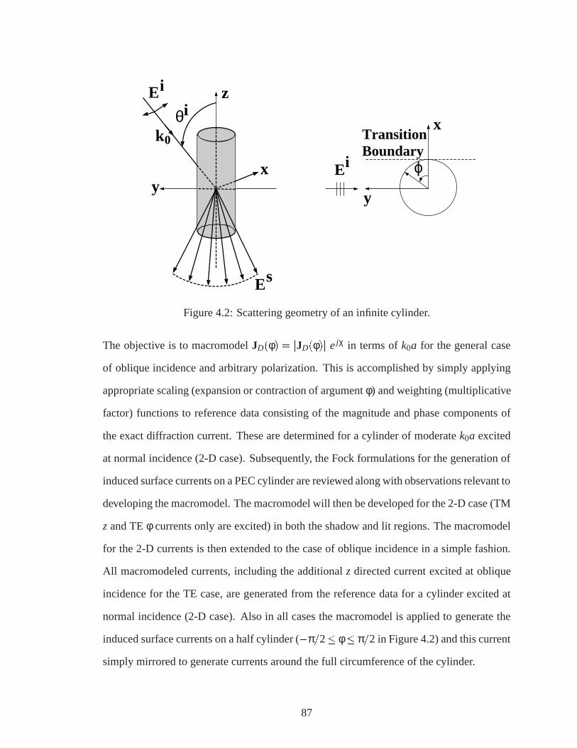
y
z
θi
x
E i
k0
E s
ϕ
x
y
Ei
TransitionBoundary
Figure 4.2: Scattering geometry of an infinite cylinder.
The objective is to macromodelJD(φ) = jJD(φ)j ejχ in terms ofk0a for the general case
of oblique incidence and arbitrary polarization. This is accomplished by simply applying
appropriate scaling (expansion or contraction of argumentφ) and weighting (multiplicative
factor) functions to reference data consisting of the magnitude and phase components of
the exact diffraction current. These are determined for a cylinder of moderatek0a excited
at normal incidence (2-D case). Subsequently, the Fock formulations for the generation of
induced surface currents on a PEC cylinder are reviewed along with observations relevant to
developing the macromodel. The macromodel will then be developed for the 2-D case (TM
z and TEφ currents only are excited) in both the shadow and lit regions. The macromodel
for the 2-D currents is then extended to the case of oblique incidence in a simple fashion.
All macromodeled currents, including the additionalz directed current excited at oblique
incidence for the TE case, are generated from the reference data for a cylinder excited at
normal incidence (2-D case). Also in all cases the macromodel is applied to generate the
induced surface currents on a half cylinder (�π=2� φ� π=2 in Figure 4.2) and this current
simply mirrored to generate currents around the full circumference of the cylinder.
87

4.2.1 Fock Theory
The macromodel of the diffraction currentJD predicts the behavior of this current as
a function ofk0a by observing the asymptotic behavior in the analytical expressions for
the Fock currents. These currents indicate the general behavior of the diffraction current
as a function ofk0a for all regions on the cylinder surface. In this section Fock theory is
reviewed and observations are made in the Fock formulations relevant to the development
of the macromodel. The analytical expressions for currents on the surface of a PEC cylinder
are given by Pathak [43]. These expressions are a special case of the Fock currents in which
the canonical Fock integrals are approximated by a Taylor series expansion in the close
neighborhood of the surface and reduce to the Fock solution on the cylinder surface. In the
shadow region the Fock currents for TM and TE cases are given by
JTMs =
iU i(Q1)
k0Z0e�ik0aφ
�k0
m
�g(ζ) z; (4.3)
JTEs = �Ui(Q1) e�ik0aφ g(ζ) φ; (4.4)
where the subscripts denotes the shadow region. In (4.3) and (4.4)Ui(Q1) is the incident
electric field for the TM case and the incident magnetic field for the TE case evaluated on
the cylinder surface at the shadow boundary (pointQ1), shown in Figure 4.1. Also in (4.3)
and (4.4),m= (k0a=2)1=3, Z0 is the characteristic impedance of free space and ˜g(ζ) and
g(ζ) are the Fock functions given by
g(ζ) =1pπ
+∞Z
�∞
dτeiζτ
w1(τ)(4.5)
g(ζ) =1pπ
+∞Z
�∞
dτeiζτ
w01(τ)
; (4.6)
88

whereζ = �mφ and is defined in the shadow region only, andw1 is the Airy function as
defined in [41]. In the lit region the Fock currents are given by
JTMl =
iU i(P)k0Z0
ei (ζ0)
3
3
�k0
m
�g(ζ0) z; (4.7)
JTEl = �Ui(P) ei (ζ
0)3
3 g(ζ0) φ; (4.8)
where the subscriptl denotes the lit region and the incident fieldUi is evaluated at the
point P on the surface of the cylinder, in the lit region, where the value of the induced
surface current is desired. In (4.7) and (4.8), ˜g and g are functions ofζ0, whereζ0 =
�msinφ and is defined in the lit region only. To construct the macromodel for the induced
surface diffraction currents the following observations of the asymptotic behavior of the
Fock currents are noted:
1. The factorm, implicit in bothζ (shadow region) andζ0 (lit region), is proportional to
(k0a)1=3.
2. In the shadow region the Fock functions for both the TM and TE cases can be eval-
uated in terms of a residue series which is a function ofζ. This indicates that the
macromodel developed for the complex diffraction current in the shadow region is
valid throughout the shadow region.
3. The TM current, given by (4.3) in the shadow region and (4.7) in the lit region, has a
weighting factor ofk0m.
4. In the deep lit region ˜g(ζ0) andg(ζ0) can be expanded into an asymptotic series given
by
g(ζ0) = 2iζ0e�i (ζ0)3
3
�1� i
4ζ03+
1
2ζ06:::
�; (4.9)
g(ζ0) = 2e�i (ζ0)3
3
�1+
i
4ζ03� 1
ζ06:::
�: (4.10)
89

5. The phase component of the Fock currents can be decomposed into a highly oscilla-
tory and slowly varying or gentle phase component. If we designate the exponential
of the diffraction current byeiχh(k0a;φ)+iχg(k0a;φ) where the subscriptsh andg indicate
the highly oscillatory and gentle phase components of the current, respectively, the
highly oscillatory phase terms are known in all regions. In the lit regionχh(k0a;φ) is
simply the phase of the incident field or
χh(k0a;φ) =�k0asinφ; (4.11)
and in the shadowχh(k0a;φ) is a linear phase term given by
χh(k0a;φ) =�k0aφ: (4.12)
The remaining gentle phase componentχg(k0a;φ) is monotonic in both the lit and
shadow regions and this is the component of the phase which will be macromodeled.
4.2.2 2-D Case, Normal Incidence
In this section the macromodel will be developed for the magnitude of the TM ˆz and
TE φ diffraction currents in the shadow region, normal incidence. The macromodel for the
diffraction current magnitude will then be extended to the lit region. Finally, the gentle
phase component will be macromodeled.
As mentioned previously, to generate diffraction currents for cylinders of arbitrary ra-
dius, the macromodels will be applied to reference data consisting of the diffraction cur-
rents from a cylinder of moderate radius, generated from the exact solution. The macro-
models described in this section are developed using reference data for the TM case from a
cylinder of radius 20λ and for the TE case a cylinder of radius 50λ. Reasons for the choice
of these cylinder sizes to generate the reference currents will be given in more detail in
90

Section 4.3.
Magnitude, Shadow region
To begin development of the macromodel for the diffraction current magnitude in the
shadow region we again note that the Fock currents in the shadow region can be evaluated
in terms of a residue series and thus the macromodel developed is valid throughout the
shadow region. Recall that the factorm is proportional to(k0a)1=3 and is implicit in the
argumentζ of both the ˜g(ζ) and g(ζ) terms in equations (4.3) and (4.4). This implies
a scaling ofφ by (k0a)1=3 for both the TM and TE cases. For the TM case, a factor of
(1=m) is observed in (4.3) implying a multiplicative or weighting factor for the TM current
of (k0a)�(1=3). Observation of (4.4) shows no weighting of the TE currents in the shadow
region. Examination of diffraction currents generated by the exact solution, however, shows
that the TM weighting factor is approximate and that there is a small weighting of the TE
currents. Empirical expressions are determined, which are functions ofk0a, to adjust for
this. Applying these scaling and weighting factors we now define the macromodel in the
shadow region, relating the diffraction current magnitudes on a cylinder of arbitrary radius
a2 to that of the reference cylinder of radiusa1 by
jJTM;TED (k0a2;φ)j= ΦTM;TE
s jJTM;TED (k0a1;
�k0a1
k0a2
�(1=3)
φ)j: (4.13)
The weighting factorΦTM;TEs is given by
ΦTM;TEs =
�k0a1
k0a2
�WTM;TEs (k0a2)
; (4.14)
whereWTM;TEs (k0a2) is approximately equal to(1=3) for the TM case and 0 for the TE
case. Expressions forWTM;TEs (k0a2) are obtained empirically from the exact solution and
91

are given by
WTMs (k0a2) =8>><>>:
0:3373+0:009562e�0:1176k0a2 +0:0045531e�0:04896k0a2 1λ < a2 < 20λ
0:3348+0:005651e�0:01103k0a2 +0:001721e�0:0024k0a2 15λ < a2 <+∞(4.15)
WTEs (k0a2) =8>>>>>><
>>>>>>:
�0:02086+0:01708(1�e�0:09979k0a2)
+0:006827(1�e�0:002576k0a2) 1λ < a2 < 50λ
�j0:005987�0:007045(1�e�0:006046k0a2)j 20λ < a2 <+∞:
(4.16)
Magnitude, Lit Region
To macromodel the magnitude of the TM ˆzand TEφ diffraction current in the lit region
we note that the behavior of the diffraction current (as a function ofk0a) transitions from
the shadow boundary to the deep lit region. To macromodel this behavior the magnitude
of the diffraction current is defined in the lit region, at and very near the shadow boundary,
and also at the deep lit region. Sigmoidal functions are then used to model the transition
from the shadow boundary to the deep lit region.
To define the magnitude of the diffraction current in the lit region at and very near the
shadow boundary for the TM case we note that in the transition from shadow to lit regions
the magnitude of the TM diffraction current is continuous across the shadow boundary
therefore (4.13) and (4.14) apply in the lit region at and very near the shadow boundary.
However, for the TE case the magnitude of the diffraction current across the transition from
shadow to lit is discontinuous. The PO current for the TE case undergoes an abrupt transi-
tion from a constant in the lit region to zero at the shadow boundary. The exact TE current
92

transitions gradually and monotonically across the shadow boundary. Remembering that
the diffraction current is defined asJD = Jex� JPO, the abrupt change in the PO current
causes a phase reversal in the TE diffraction current and an abrupt change in the magnitude
of the TE diffraction current across the shadow boundary. This can be seen in Figure 4.3b.
It was determined empirically from the exact solution that near the shadow boundary in
the lit region, (4.13) and (4.14) can be applied for the TE case if the factorWTEs (k0a2) is
modified as follows:
WTEl ;sb(k0a2) =�2:25WTE
s (k0a2); (4.17)
where the subscriptl ;sb implies the lit region at the shadow boundary.
To define the magnitude of the diffraction currents in the deep lit region recall that in the
deep lit region the surface currents are described by the asymptotic expansions of the Fock
functions,g(ζ0) andg(ζ0) given in (4.9) and (4.10). The first terms in (4.9) and (4.10) are
the PO currents, with higher order terms defining the non-uniform or diffraction currents.
In the deep lit region only the second term in (4.9) and (4.10) are needed to evaluate the
diffraction current. Substituting the second term in (4.9) and (4.10) for ˜g(ζ0) andg(ζ0) in
(4.7) and (4.8) and evaluating the resulting expressions indicates that the diffraction current
in the deep lit region is weighted by a coefficient of 1=(k0a), implicit in the (ζ0)3 term in
the denominator of the second term in (4.9) and(4.10) (recall that,m= (k0a=2)1=3). There
is no scaling of the argumentφ in the deep lit region for either the TM or TE case.
Having established the behavior of the diffraction current magnitudes at the shadow
boundary and in the very deep lit region, a function must be specified to transition from
the shadow boundary to the deep lit region. In a manner similar to the shadow region we
first define the relationship between the diffraction current magnitude in the lit region on a
93
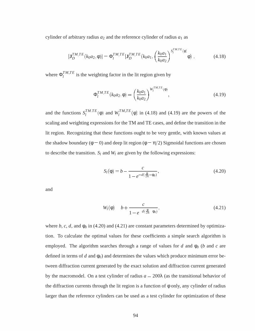
cylinder of arbitrary radiusa2 and the reference cylinder of radiusa1 as
jJTM;TED (k0a2;φ)j= ΦTM;TE
l jJTM;TED (k0a1;
�k0a1
k0a2
�STM;T El (φ)
φ)j; (4.18)
whereΦTM;TEl is the weighting factor in the lit region given by
ΦT M;TEl (k0a2;φ) =
�k0a1
k0a2
�WTM;T El (φ)
; (4.19)
and the functionsSTM;TEl (φ) andWTM;TE
l (φ) in (4.18) and (4.19) are the powers of the
scaling and weighting expressions for the TM and TE cases, and define the transition in the
lit region. Recognizing that these functions ought to be very gentle, with known values at
the shadow boundary (φ = 0) and deep lit region (φ = π=2) Sigmoidal functions are chosen
to describe the transition.Sl andWl are given by the following expressions:
Sl(φ) = b� c
1+e�d( φ2π�φ0)
; (4.20)
and
Wl (φ) = b+c
1+e�d( φ2π�φ0)
; (4.21)
whereb, c, d, andφ0 in (4.20) and (4.21) are constant parameters determined by optimiza-
tion. To calculate the optimal values for these coefficients a simple search algorithm is
employed. The algorithm searches through a range of values ford andφ0 (b andc are
defined in terms ofd andφ0) and determines the values which produce minimum error be-
tween diffraction current generated by the exact solution and diffraction current generated
by the macromodel. On a test cylinder of radiusa= 200λ (as the transitional behavior of
the diffraction currents through the lit region is a function ofφ only, any cylinder of radius
larger than the reference cylinders can be used as a test cylinder for optimization of these
94

parameters), the optimal values ofb, c, d, φ0 are determined and are given in Table 4.1,
with the exception of theb andc coefficients for forWTM;TEl defined asbTM
w , bTEw , cTM
w and
cT Ew in Table 4.1. At the shadow boundaryWTM
l is defined byWTMs andWTE
l is defined by
WTEl ;sb (WTE
l defined at the shadow boundary given in (4.17)), making both functions ofk0a.
These coefficients as functions ofk0a are given by
cTMw = (1�WTM
s )
�1
1+e�d(1�φ0)� 1
1+edφ0
��1
(4.22)
cTEw = (1�WTE
l ;sb)
�1
1+e�d(1�φ0)� 1
1+edφ0
��1
(4.23)
bTM;TEw = 1�cT M;TE
w
�1
1+e�d(1�φ0)
�: (4.24)
Table 4.1: Optimized parameters for Sigmoidal transition functions
d φ0 b c
STMl (φ) 9.903 0.5650 0.3346 0.3391
STEl (φ) 10.6 0.6630 0.3336 0.3430
WTMl (k0a;φ) 10.025 0.5268 bTM
w cT Mw
WTEl2 (k0a;φ) 8.5 0.610 bTE
w cT Mw
Phase, All Regions
Having developed an accurate model for the magnitude of the complex diffraction cur-
rent the next step is to macromodel the gentle phase component for the 2-D case. This gen-
tle phase component,χg(k0a;φ), is monotonic for the TM case and piecewise monotonic
for the TE case as shown in Figures 4.4a and 4.4b, respectively. The observed behavior
95

of the Fock currents again allows for prediction of the asymptotic behavior of this gentle
phase factor in an accurate fashion. As already noted, in the shadow region a residue se-
ries is applied to calculate the complex surface currents. Recall that this residue series is a
function ofζ which again implies a scaling of the argumentφ, implicit in ζ, by (k0a)(1=3)
for both the TM and TE cases. This scaling was determined to be valid for the gentle phase
function in the shadow region. In addition, it was also determined empirically that this scal-
ing is an acceptable approximation in the lit region. While no weighting of the gentle phase
component is implied by observation of the Fock currents it was observed empirically that
a small offset ofχg(k0a;φ) as a function ofk0a is necessary and this offset is determined by
observation of the exact solution. Thus the expression relating the gentle phase component
for a cylinder of radiusa2 to the reference cylinder of radiusa1 is
χTM;TEg (ka2;φ) = OTM;TE+χTM;TE
g (ka1;
�k0a1
k0a2
�(1=3)
φ); (4.25)
whereOTM;TE is the adjustment factor for the gentle phase term and is given for the TM
case in all regions and the TE case in the shadow region by
OTM;TE(k0a2) = 8>>>>>>>>>><>>>>>>>>>>:
0:07255�0:05857(1�e�0:08778k0a2)
�0:01777(1�e�0:01231k0a2) 1λ < a2 < 20λ
0:01608�0:01701(1�e�0:01592k0a2)
�0:005747(1�e�0:002158k0a2) 15λ < a2 <+∞;
(4.26)
As mentioned earlier the PO current for the TE case undergoes an abrupt transition at
the shadow boundary causing a phase reversal in the diffraction current. Thus,χTEg is
discontinuous across the shadow boundary as can be seen in Figure 4.4b. Consequently,
OTE is also discontinuous across the shadow boundary. The relationship betweenOTE in
96
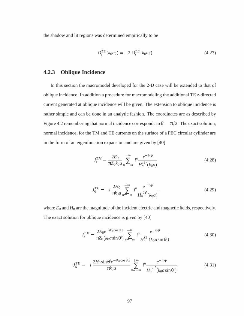
the shadow and lit regions was determined empirically to be
OTEl (k0a2) =�2 OTE
s (k0a2): (4.27)
4.2.3 Oblique Incidence
In this section the macromodel developed for the 2-D case will be extended to that of
oblique incidence. In addition a procedure for macromodeling the additional TEz-directed
current generated at oblique incidence will be given. The extension to oblique incidence is
rather simple and can be done in an analytic fashion. The coordinates are as described by
Figure 4.2 remembering that normal incidence corresponds toθi = π=2. The exact solution,
normal incidence, for the TM and TE currents on the surface of a PEC circular cylinder are
in the form of an eigenfunction expansion and are given by [40]
JTMz =
2E0
πZ0k0a
+∞
∑n=�∞
ine�inφ
H(2)n (k0a)
(4.28)
JTEφ =�i
2H0
πk0a
+∞
∑n=�∞
ine�inφ
H(2)n
0(k0a)
; (4.29)
whereE0 andH0 are the magnitude of the incident electric and magnetic fields, respectively.
The exact solution for oblique incidence is given by [40]
JTMz =
2E0e�ik0 cosθiz
πZ0(k0asinθi)
+∞
∑n=�∞
ine�inφ
H(2)n (k0asinθi)
(4.30)
JTEφ =�i
2H0sinθie�ik0 cosθiz
πk0a
+∞
∑n=�∞
ine�inφ
H(2)n
0(k0asinθi)
; (4.31)
97

It is evident in the relation of (4.30) and (4.31) to (4.28) and (4.29) that surface currents
for the case of oblique incidence can be obtained from those of normal incidence with the
following modifications:
� k0a! k0asinθi ; incident wave simply “sees” an effectively smaller cylinder
� a multiplicative, progressive phase factor,e�ik0 cosθiz is added
� TE current is modified by sinθi (projection factor)
An additionalz - directed current is generated for the TE case at oblique incidence
angles. This current is not independent and its dependence onJTEφ (k0a;φ;θi) is given by
[40]
JTEz (k0a;φ;θi) =
�i cotθi
k0asinθi
∂∂φ
JTEφ (k0a;φ;θi): (4.32)
Having an expression forJTEφ (k0a;φ;θi), the expression forJTE
z (k0a;φ;θi) can be obtained.
However, remembering thatJTEφ (k0a;φ;θi) is composed of a PO component,JTE
POφ(k0a;φ;θi)
and a diffraction component,JTEDφ (k0a;φ;θi), the magnitude and phase ofJTE
Dφ (k0a;φ;θi) is
macromodeled separately and evaluation of∂∂φJTE
Dφ (k0a;φ;θi) is not straightforward. A pro-
cedure is outlined for the calculation of∂∂φJTE
Dφ (k0a;φ;θi).
As mentioned, in order to generateJTEz (k0a;φ;θi), the term ∂
∂φJTEDφ (k0a;φ;θi) must be
evaluated in terms of the macromodel. The expression forJTEDφ (k0a;φ;θi) in terms of the
macromodel is of the form given by (4.13), (4.18) and (4.25) or
JTEDφ (k0a2;φ) =ΦTE jJTE
Dφ (k0a1;
�k0a1
k0a2
�STE(k0a2;φ)φ)j
efiOTE(k0a2)+iχTE
g (k0a1;(k0a1k0a2
)(1=3)
φ)geiχh(k0a2;φ):
(4.33)
98

The derivative of (4.33) with respect toφ, in terms of the macromodel, is straightforward
with the exception of two terms. These terms are the derivatives of the magnitude and gentle
phase component of the reference cylinder, and their evaluation in terms of the macromodel
is not obvious. These terms are given by:
∂∂φjJTE
Dφ (k0a1;
�k0a1
k0a2
�STE(k0a2;φ)φ)j= ∂
∂φjJTE
Dφ (k0a1; φ)j � ∂φ∂φ
(4.34)
where
φ =
�k0a1
k0a2
�STE(k0a2;φ)φ (4.35)
and
∂∂φ
χTEg (k0a1;
�k0a1
k0a2
�(1=3)
φ) =�
k0a1
k0a2
�(1=3) ∂∂φ
χTEg (k0a1; φ) (4.36)
whereSTE in (4.34) is the scaling factor for the TE case, given by 1=3 in the shadow region
and the Sigmoidal transition functionSTEl in the lit region, as described previously. While
evaluation of the∂φ∂φ in (4.34) is simple, evaluation of the other derivatives to the right of the
equal sign in (4.34) and (4.36) is not. To evaluate these terms we note that∂∂φ jJTE
Dφ (k0a1; φ)jand ∂
∂φχTEg (k0a1; φ) in (4.34) and (4.36) are derivatives of the entire argument and are there-
fore independent ofk0a. We can therefore calculate these terms directly from diffraction
current in the reference data. To do this we simply define the diffraction current in terms of
its real and imaginary parts orJTEDφ = X+ iY. The derivative of the magnitude is then given
by
∂∂φjJTE
Dφ j=XX0+YY0
pX2+Y2
; (4.37)
99

and the derivative of the phase by
∂∂φ
χTEg =
Y0X�YX0
X2+Y2 : (4.38)
4.3 Validation: PEC Cylinder
In the previous section a macromodel was developed which relates the diffraction cur-
rent on a PEC cylinder of arbitrary radiusa2 to that of a reference cylinder of radiusa1,
for plane wave excitation. In practice this macromodel allows the complex diffraction cur-
rents for any cylinder with radiusa2 illuminated by a plane wave at oblique incidence to be
generated from the diffraction current for a reference cylinder of radiusa1 when excited at
normal incidence. The reference data is generated using the exact solution for a cylinder
with a moderate value ofk0a. In this section the validity and accuracy of the macromodel is
examined by comparing the surface currents and near fields generated by the eigensolution
with those of the macromodel for cylinders of radii larger than 1λ. Figure 4.3 shows the
macromodeled diffraction current magnitude for cylinders of radii 10λ and 100λ excited
at normal incidence compared to the exact solution for the TM case (a) and the TE case
(b). The horizontal axes in both figures are the normalized angular dimension orφ=2π with
φ=2π = 0; 0:5 corresponding to the top and bottom shadow boundaries respectively.
As mentioned previously, the reference cylinder radiusa1 was chosen to be 20λ for
the TM case and 50λ for the TE case. The choice of radius for the reference cylinder is
somewhat subjective but the main criteria was the negligible level of the ripple in the mag-
nitude and gentle phase components of the exact diffraction current in the deep shadow.
The diffraction current magnitude component in the deep shadow show a rapid oscilla-
tion (ripple) (as seen in Figure 4.3) which is due to the effects of higher order diffraction
(multiple transitions of the creeping wave around the cylinder). The gentle phase compo-
nent exhibits similar behavior but at a much lower level. As cylinder radius increases the
100

−0.2 0 0.2 0.4 0.6
−200
−150
−100
−50
0
φ/2π
Dz
20 lo
g(|J
TM
|)10λ100λ
(a) jJTMDz j
−0.2 0 0.2 0.4 0.6−120
−100
−80
−60
−40
−20
0
φ/2π
20 lo
g(|J
TE φ|
)
10λ
100λD
(b) jJTEDφ j
Figure 4.3: Diffraction current magnitude (dB) around full circumference of 10 and 100λPEC cylinders excited at normal incidence angle,θi = π=2, eigensolutioncurrent (———–), compared with macromodeled current (- - - - - -), φ
2π = 0is equivalent to a point on top of the cylinder, perpendicular to the shadowboundary, with φ
2π =�0:25 in the deep shadow region.
frequency of the ripple increases and becomes more localized to the deep shadow region
(φ=2π = �0:25 in Figure 4.3). It should be noted that the level of diffraction current at
which this ripple takes place is very low and therefore it is unlikely that this ripple would
affect the near field anywhere except perhaps very near the surface in the deep shadow.
Because this ringing cannot be macromodeled a reference cylinder radius was chosen to
minimize the error between the exact solution and the macromodel for any cylinder radius
greater than 1λ. In the reference data this ripple is removed from both the magnitude and
gentle phase components of the diffraction current and the remaining curve extended by
assuming a continuation of the slope of the remaining data. The macromodeled diffraction
current for the TE case (Figure 4.3b) shows noticeable error for the 10λ cylinder in the deep
lit region (φ=2π = 0:25) and is attributed to increasing error in the value of the weighting
factor Φ, for decreasingk0a. In this region the PO current is dominant however and the
error in the total current is still within the values described previously. In practice this has
no effect on the accuracy of the total fields.
The error between the exact solution and the macromodel was investigated from a cylin-
101

−0.2 0 0.2 0.4 0.6
−700
−600
−500
−400
−300
−200
−100
0
φ/2π
f gf (
Deg
rees
)
(a) χTMg
−0.2 0 0.2 0.4 0.6−150
−100
−50
0
50
100
150
200
φ/2π
f gf (
Deg
rees
)
(b) χTEg
Figure 4.4: Gentle phase component (degrees) around full circumference of 10 and 100λPEC cylinders excited at normal incidence angle,θi = π=2, 10λ (———–),100λ (- - - - - -), φ
2π = 0 is equivalent to a point on top of the cylinder,
perpendicular to the shadow boundary, withφ2π = �0:25 in the deep shadow
region.
der of 1λ radius up to a cylinder with radius of 200λ. In this range the maximum error in
magnitude in the total current (PO + diffraction) was -60 dB where the magnitude error is
as previously defined or,ejj = 20log(jjJexj� jJmmjj). The phase error over this range was
found to be less than 0:1Æ near the shadow boundary. Figure 4.5 shows an example of the
macromodeled total current for a 100λ PEC cylinder excited at oblique incidenceθi = π=4
as compared to the exact current. Figure 4.5a and Figure 4.5b show the magnitude and
phase, respectively, of the total current for the TM case. Figure 4.5c shows the TEφ - di-
rected current with Figure 4.5d showing the additionalz - directed current for the TE case
at oblique incidence angle. As can be seen the macromodel agrees very well with the exact
solution in all cases.
The accuracy of the total fields (incident + scattered) generated by the macromodeled
currents is shown in Figure 4.6a for the TM case and Figure 4.6b for the TE case. The
data shown is for a 100λ cylinder excited at oblique incidence,θi = π=4, with fields 1λ
102

off the cylinder surface plotted. Results from the macromodel are again compared with
the exact solution. The scattered fields for both solutions are generated by applying the
radiation integrals to the exact and macromodeled total currents. The fields generated by
the macromodel are in good agreement over the entire range shown for both the TM and
TE cases. The macromodel was shown to produce near fields which are highly accurate
over a dynamic range of greater than 85 dB for cylinders of up to 200λ radius. The one
exception to this is the TEφ - directed near fields at oblique incidence. As the incidence
angle approaches grazing the TE PO current is attenuated by a sinθi factor. As this happens
the accuracy of the TEφ - directed near fields is degraded. In the near field however the TE
ρ - directed field is the dominate field component and the total field retains the high degree
of accuracy previously shown.
4.3.1 Direct Evaluation of Fock Type Integrals
As mentioned in the introductory section direct numerical evaluation of the Fock inte-
grals is difficult due to their highly oscillatory nature. At this point it is relevant to compare
results generated by direct numerical evaluation of these integrals to the proposed macro-
model. We begin by observing the TM and TE current distributions, for cylinders of radius
10, 15, and 20λ, and generated by the Fock type integrals as seen in Figure 4.7. What is
apparent in these curves is the convergence problems of the Fock type integrals in the deep
lit region, and the increasing region of non-convergence as cylinder radius increases. As
cylinder radius is increased the integrand becomes more oscillatory, and evaluation of the
Airy type functionsw1;w01 in (4.5) and (4.6), more difficult. Convergence of the integrand
for larger radius requires evaluation of the integrand for larger argument ofw1. As the ar-
gument ofw1 increases it value increases exponentially (see [41]) and the numerical error
in evaluating the integrand grows significantly, thus making convergence difficult. This
correlates with the discontinuity between transitioning from tabulated data generated in the
lit region towards the shadow boundary [47], to the asymptotic solution applied in the deep
103
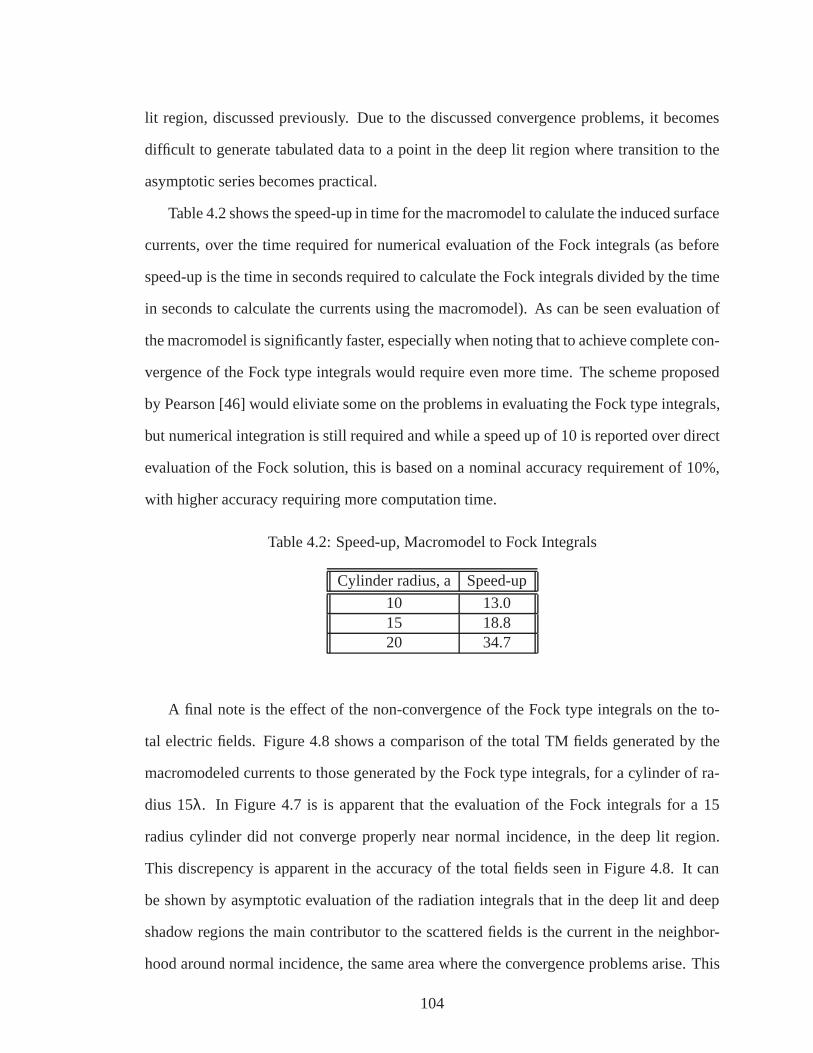
lit region, discussed previously. Due to the discussed convergence problems, it becomes
difficult to generate tabulated data to a point in the deep lit region where transition to the
asymptotic series becomes practical.
Table 4.2 shows the speed-up in time for the macromodel to calulate the induced surface
currents, over the time required for numerical evaluation of the Fock integrals (as before
speed-up is the time in seconds required to calculate the Fock integrals divided by the time
in seconds to calculate the currents using the macromodel). As can be seen evaluation of
the macromodel is significantly faster, especially when noting that to achieve complete con-
vergence of the Fock type integrals would require even more time. The scheme proposed
by Pearson [46] would eliviate some on the problems in evaluating the Fock type integrals,
but numerical integration is still required and while a speed up of 10 is reported over direct
evaluation of the Fock solution, this is based on a nominal accuracy requirement of 10%,
with higher accuracy requiring more computation time.
Table 4.2: Speed-up, Macromodel to Fock Integrals
Cylinder radius, a Speed-up
10 13.015 18.820 34.7
A final note is the effect of the non-convergence of the Fock type integrals on the to-
tal electric fields. Figure 4.8 shows a comparison of the total TM fields generated by the
macromodeled currents to those generated by the Fock type integrals, for a cylinder of ra-
dius 15λ. In Figure 4.7 is is apparent that the evaluation of the Fock integrals for a 15
radius cylinder did not converge properly near normal incidence, in the deep lit region.
This discrepency is apparent in the accuracy of the total fields seen in Figure 4.8. It can
be shown by asymptotic evaluation of the radiation integrals that in the deep lit and deep
shadow regions the main contributor to the scattered fields is the current in the neighbor-
hood around normal incidence, the same area where the convergence problems arise. This
104

is evident in Figure 4.8 as the most significant error between the total fields generated by
the Fock integrals when compared to those generated by the macromodel can be seen in
these regions.
4.4 Application of Macromodel
To summarize the techniques described in the previous sections, the following steps are
applied to calculated the induced surface currents on a PEC cylinder using the proposed
macromodel:
1. Generate reference data at normal incidence (a= 20λ for TM, a= 50λ for TE) us-
ing the exact solution. Remove oscillations in reference data in deep shadow and
approximate by extending slope of remaining data.
2. Apply equations (4.13) through (4.16) and (4.17) through (4.24) to the magnitude of
the reference data for normal incidence to generate the magnitude of the diffraction
current in the shadow and lit regions, respectively, for a cylinder of the desired radius.
3. Apply equations (4.25) through (4.27) to the gentle phase component of the reference
data for normal incidence to generate the gentle phase component in the shadow and
lit regions, respectively.
4. To generate the TM ˆz and TE φ currents for oblique incidence simply apply the
modifications given in Section 4.2.3. For the additionalz directed current generated
at oblique incidence for the TE case apply (4.32) through (4.38) to the reference data
for normal incidence to generate the derivative of theφ directed current needed.
5. Reference cylinder data is compressed onφ axis when macromodeling surface diffrac-
tion current on cylinders of larger radius than that of the reference cylinder. Because
of this the macromodeled data does not extend over full range of cylinder (deep
105

shadow to deep lit). To extend the macromodeled data to the full extent of the cylin-
der simply assume a continuation of the slope in the lit and shadow regions, respec-
tively.
6. If higher sampling of diffraction currents is required apply simple linear interpola-
tion to the magnitude and gentle phase component of the macromodeled current to
generate additional data points.
4.5 Other Applications
The ability to accurately predict the scattered fields from a circular cylinder or any
general convex surface has applications other than those of interest in this thesis and at this
point it is appropriate to give some mention of them. In radar applications the proposed
method could be used to evaluate the detectability of hidden targets behind a hill or knoll.
In an extension to applications in wireless communication the macromodel can be applied
to evaluate the field pattern of antennas mounted on structures of circular cross-section. As
an example of this consider a small dipole mounted on an aircraft fuselage. By application
of reciprocity [48] source and observation can be exchanged, and the case of plane wave
incidence-near field observation, examined thus far, can be applied to evaluate the far-fields
generated from a point source (small dipole) radiating in the presence of a convex surface. It
can be shown through reciprocity that for identical point sources the following relationship
holds:
l1 �E2 = l2 �E1; (4.39)
whereE1; E2 are electric fields caused by point sources with orientationl1, l2, respectively.
If l1 is radiating in the far-field of the convex surface and the corresponding electric field
E1 is observed in the near-field of the surface it is equivalent to the plane wave excitation
106

problem with the incident plane wave weighted by the dipole field coefficients given by
Eid(r) =
�il1k0Z0I04πr
eik0r [I � ki1 � l1ki
1]; (4.40)
where the vectorr = r r is defined from the axis origin (always at the origin of the local
radius of curvature) to the dipole position,l1 is the dipole length, andI0 is the dipole
current magnitude. Ifl2 is the orientation of a dipole radiating in the near-field of the
convex surface and knowing the plane wave solution (4.39) can be solved for fieldsE2
which are the far-fields generated by an infinitesimal dipole radiating in the presence of a
convex surface. Applying this technique, far-field results for the 2-D case were generated
for an infinitesimal dipole radiating in the presence of a 20λ circular PEC cylinder which
can represent the fuselage of an aircraft (12m diameter at 1 GHz). The dipole is positioned
at the top of the fuselage (x axis, coordinates in Figure 4.2 apply), 0:1λ away from the
surface. Figure 4.9 the shows the far-field patterns for three dipole orientations along with
their corresponding positions. Figure 4.9a shows the result from ax - directed point source
with Figures 4.9b and 4.9c showing the results from ay and z - directed dipole. Again the
fields generated from the macromodel are in excellent agreement with those generated by
the exact solution.
4.6 Chapter Summary: Diffraction from Right Circular
Cylinders
Motivated by the shortcomings in existing high frequency techniques, an alternative
method was sought to calculate the diffraction and scattering from general convex sur-
faces. In this chapter the case of right circular cylinders was examined and a macromodel
developed, based on PTD and Fock analysis, which predicts the diffraction currents in-
duced on the surface of electrically large cylinders when excited by a plane wave at oblique
107

angles. The case of a PEC cylinder was examined and an approach to determining these
diffraction currents was presented which is based on the asymptotic behavior of the Fock
currents. The method is highly accurate, producing total near fields with a dynamic range
of over 85 dB. The macromodel developed is algebraic in nature and simple to implement.
In the next chapter the macromodel developed is extended to include the case of general
convex surfaces, when excited at oblique angles. The macromodeled currents are extended
to a convex surface in the standard manner of applying the currents induced on a circular
cylinder locally on the convex surface.
108

−0.2 0 0.2 0.4 0.6
−200
−150
−100
−50
0
φ/2π
20 lo
g(|J
TM
z|)
(a) jJTMz j
−0.01 −0.005 0 0.005 0.01
−150
−100
−50
0
50
100
150
φ/2π
∠ J
TM
z (
Deg
rees
)
(b)\JTMz j
−0.2 0 0.2 0.4 0.6−120
−100
−80
−60
−40
−20
0
φ/2π
20 lo
g(|J
TE φ|)
(c) jJTEφ j
−0.2 0 0.2 0.4 0.6−100
−80
−60
−40
−20
0
20 lo
g(|J
TE
z|)
φ/2π
(d) jJTEz j
Figure 4.5: Total current, magnitude (dB) and phase (degrees) around full circumference ofa 100λ PEC cylinder excited at oblique incidence angle,θi = π=4, eigensolutioncurrent (———–), compared with macromodeled current (- - - - - -), φ
2π = 0is equivalent to a point on top of the cylinder, perpendicular to the shadowboundary, with φ
2π = �0:25 in the deep shadow region. (a) and (b) aremagnitude and phase of TMz - directed current with (c) and (d) magnitudeof TE φ andz - directed current respectively.
109
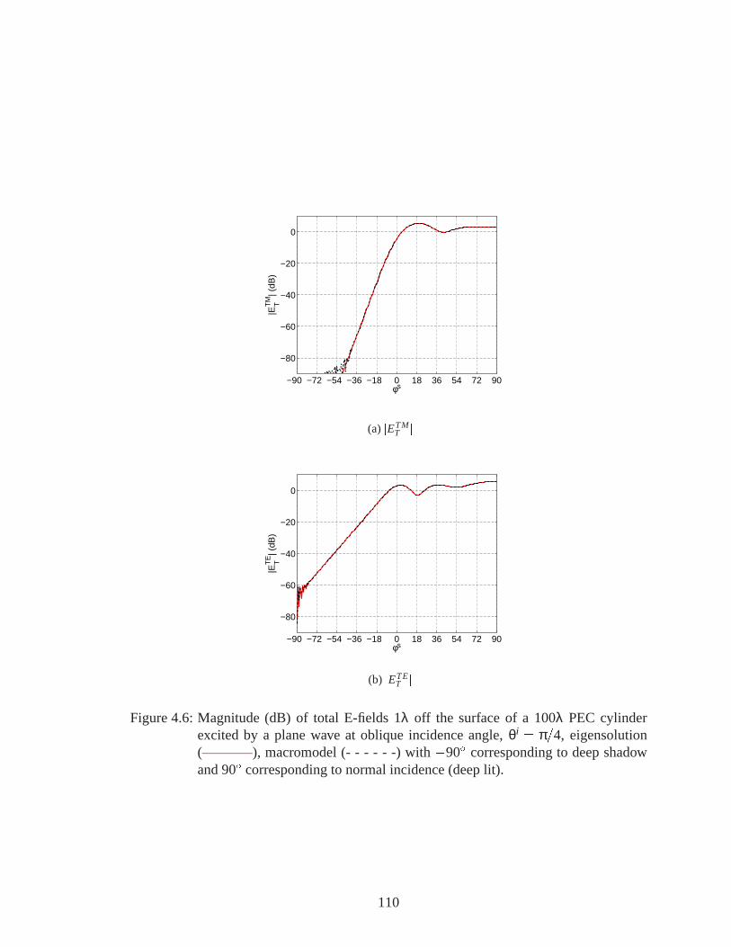
−90 −72 −54 −36 −18 0 18 36 54 72 90
−80
−60
−40
−20
0
|ETT
M| (
dB)
φs
(a) jETMT j
−90 −72 −54 −36 −18 0 18 36 54 72 90
−80
−60
−40
−20
0
|ETT
E| (
dB)
φs
(b) jETET j
Figure 4.6: Magnitude (dB) of total E-fields 1λ off the surface of a 100λ PEC cylinderexcited by a plane wave at oblique incidence angle,θi = π=4, eigensolution(———–), macromodel (- - - - - -) with�90Æ corresponding to deep shadowand 90Æ corresponding to normal incidence (deep lit).
110

−0.2 0 0.2 0.4 0.6−100
−80
−60
−40
−20
0
20
40
φ/2π
20 lo
g(|J
TM
z|)
(a) jJTMz j
−0.2 0 0.2 0.4 0.6−50
−40
−30
−20
−10
0
10
20
30
40
50
φ/2π
20 lo
g(|J
TE φ|)
(b) jJTEφ j
Figure 4.7: Total current magnitude (dB) of Fock currents around full circumference of aPEC cylinder excited at normal incidence angle,θi = π=2, a= 10λ (———–),a= 15λ (- - - - - -), a= 20λ (� � � � �). φ
2π = 0 is equivalent to a point on
top of the cylinder, perpendicular to the shadow boundary, withφ2π =�0:25 in
the deep shadow region.
111
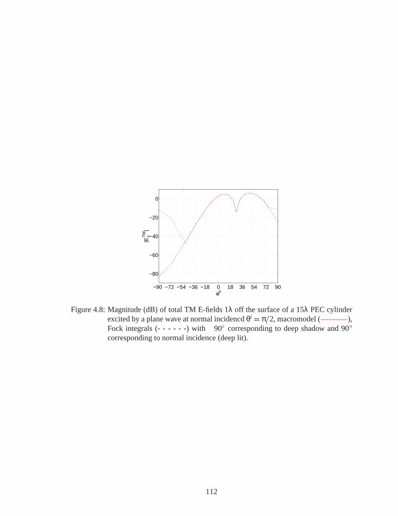
−90 −72 −54 −36 −18 0 18 36 54 72 90
−80
−60
−40
−20
0
|ETT
M|
φs
Figure 4.8: Magnitude (dB) of total TM E-fields 1λ off the surface of a 15λ PEC cylinderexcited by a plane wave at normal incidencdθi = π=2, macromodel (———–),Fock integrals (- - - - - -) with�90Æ corresponding to deep shadow and 90Æ
corresponding to normal incidence (deep lit).
112

90
30
210
60
240
270
120
300
150
330
180
0
−120−105−90−75−60−45−30−150
(a) jEsφj, Far-field,x - directed dipole
90
30
210
60
240
270
120
300
150
330
180
0
−120−105−90−75−60−45−30−150
(b) jEsφj, Far-field,y - directed dipole
90
30
210
60
240
270
120
300
150
330
180
0
−120−105−90−75−60−45−30−150
●
(c) jEszj, Far-field,z - directed dipole
Figure 4.9: Magnitude (dB) of total far-fields generated by a point source (small dipole)radiating in the presence of a 20λ PEC cylinder positioned 0:1λ off cylindersurface along thex axis (0Æ in plot) at z = 0. Observation is at 2(2a)2=λfrom cylinder center and inx� y plane atz = 0, eigensolution (———–),macromodel (- - - - - -).
113
CHAPTER 5
Diffraction from Convex Surfaces
In the preceding chapter a novel approach, based on the Physical Theory of Diffraction
(PTD) and Fock theory was developed to macromodel the induced surface currents on a
right circular, PEC cylinder, when excited by a plane wave. The proposed method generated
highly accurate surface currents without the need for complex mathematical analysis, or
numerical evaluation of integrals. For the case of a general convex surface, infinite in one
dimension, and with large, slowly varying radius of curvature, the induced surface currents
on a circular cylinder can be applied locally to approximate those induced on the convex
surface. In this chapter the macromodel for the induced surface currents on a right circular
PEC cylinder will be applied to approximate the currents induced on a general convex
surface, infinite in one dimension, which can represent the effect of natural obstacles, such
as hills, mountains, or ridgelines on the propagating radio wave. In the sections that follow
the macromodel will be extended to a general convex surface in a standard way, as found
in the literature [43], by applying the induced surface currents from a circular cylinder
locally, on the convex surface. To validate the technique on a non-circular cylinder, results
are generated for the fields scattered from an elliptical cylinder using the macromodeled
currents and compared to those generated by a Method of Moments (MoM) numerical
code. Curves are then shown for the fields scattered by a parabolic hill and compared to
those generated using the Kirchhoff (knife-edge) diffraction method.
114

5.1 Introduction
As mentioned in the previous chapter, many natural terrain features exhibit both curved
and doubly curved surfaces. Ridgelines in mountainous areas can exhibit the features of a
long, singly curved surface (see Figure 5.1), which is essentially infinite in one dimension.
Current methods of propagation prediction for natural obstacles tend to be either overly
Figure 5.1: Ridgelines in Mountainous Region
simplistic, such as Kirchhoff (knife-edge) diffraction, or do not account for the curvature
of the obstacle, such as wedge diffraction. High frequency techniques, while accounting
for the radius of curvature of the obstacle, are mathematically complex, and can be numer-
ically cumbersome, as was seen in the last chapter in evaluating the Fock type integrals for
induced surface currents. In addition techniques such as the Uniform Theory of Diffrac-
tion (UTD) have been shown to have serious limitations in accuracy, and in essence are not
asymptotic in the high frequency limit, as cylinder radius increases. Details of the problems
and limitations of these techniques have been throughly discussed in the previous chapter
and will not be repeated here. Suffice to say that the need for an alternate method to pre-
dict scattering and diffraction from convex surfaces of large radius of curvature is apparent.
With this as a motivation a macromodel for the induced surface currents on a PEC right
circular cylinder was developed in the last chapter. The proposed macromodel is simple,
easy to implement, and most important, shown to be highly accurate. In this chapter the
115

macromodeled currents from the circular cylinder will be applied in a standard fashion, to
approximate the induced surface currents on a singly curved (infinite in one dimension)
convex surface, with large slowly varying radius of curvature.
5.2 Induced Surface Currents: General Convex Surface
The macromodel for the surface currents induced on a right circular PEC cylinder, when
excited by a plane wave, are extended to that of a general convex surface by assuming that
the surface currents induced on the convex surface can be approximated locally by those
induced on a circular cylinder. This is a valid approximation provided that the convex sur-
face is of large, slowly varying radius of curvature. To extend the macromodel to a general
convex surface, and referring to the geometry as shown in Figure 5.2, modifications are
made to the following parameters, defined in the previous chapter for the circular cylinder.
Ei
P
P
●
Q1●
●x
y ϕi
β
βn
t
l
s
Figure 5.2: Geometry of a General Convex Surface
116

In all regions:
Circular Cylinder:
m=
�k0a2
�(1=3)
(5.1)
General Convex Surface:
m(rc(P)) =
�k0rc(P)
2
�(1=3)
; (5.2)
whererc(P) is the local radius of curvature of the surface, evaluated at some pointP on
the surface, and wherePl andPs indicate the pointP evaluated in the lit region, or shadow
region, respectively.
In the lit region:
Circular Cylinder:
Z0 =�mcosφ (5.3)
General Convex Surface:
Z0 =�mcosβ; (5.4)
whereβ is the angle between the incident ray and the surface normal.
In the shadow region:
Circular Cylinder:
Z =�mφ (5.5)
117

General Convex Surface:
Z =
PsZ
Q1
m(rc(τ))rc(τ)
dτ =�
k0
2
�1=3 PsZ
Q1
dτrc(τ)2=3
; (5.6)
t =
PsZ
Q1
dτ; (5.7)
γ =�
rc(Ps)
rc(Q1)
�1=6
: (5.8)
On a general convex surface the creeping wave sheds energy as a function of arclength
(parameterτ in (5.6)), thus (5.6) is the more general equation, valid for any convex surface
and reduces to (5.5) for the special case of a right circular cylinder. In (5.7)t is the arclength
along the convex surface from the shadow boundary at pointQ1 to Ps, andγ in (5.8) is
a multiplicative factor applied in the shadow region so that the Fock currents reduce to
Keller’s Geometrical Theory of Diffraction (GTD) formulation in the deep shadow region
[42, 43]. It is not clear in the literature how the parameterγ is arrived at, either by derivation
or empirically, only that it is necessary for the expressions in the deep shadow to uniformly
reduce to Keller’s solution.
5.3 Results: Diffraction from Convex Surfaces
5.3.1 Ellipse
To validate the extension of the macromodeled surface currents to a general convex
surface, the technique will first be applied to an elliptical cylinder, for the 2-D case (θi =
118
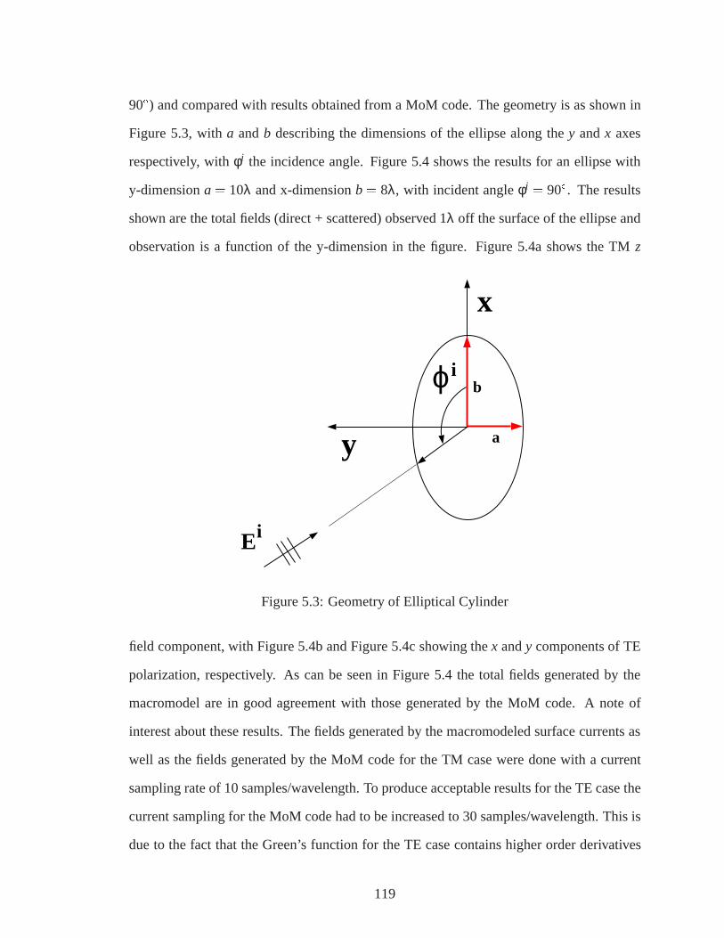
90Æ) and compared with results obtained from a MoM code. The geometry is as shown in
Figure 5.3, witha andb describing the dimensions of the ellipse along they andx axes
respectively, withφi the incidence angle. Figure 5.4 shows the results for an ellipse with
y-dimensiona = 10λ and x-dimensionb = 8λ, with incident angleφi = 90Æ. The results
shown are the total fields (direct + scattered) observed 1λ off the surface of the ellipse and
observation is a function of the y-dimension in the figure. Figure 5.4a shows the TMz
x
y
Ei
ϕi
a
b
Figure 5.3: Geometry of Elliptical Cylinder
field component, with Figure 5.4b and Figure 5.4c showing thex andy components of TE
polarization, respectively. As can be seen in Figure 5.4 the total fields generated by the
macromodel are in good agreement with those generated by the MoM code. A note of
interest about these results. The fields generated by the macromodeled surface currents as
well as the fields generated by the MoM code for the TM case were done with a current
sampling rate of 10 samples/wavelength. To produce acceptable results for the TE case the
current sampling for the MoM code had to be increased to 30 samples/wavelength. This is
due to the fact that the Green’s function for the TE case contains higher order derivatives
119
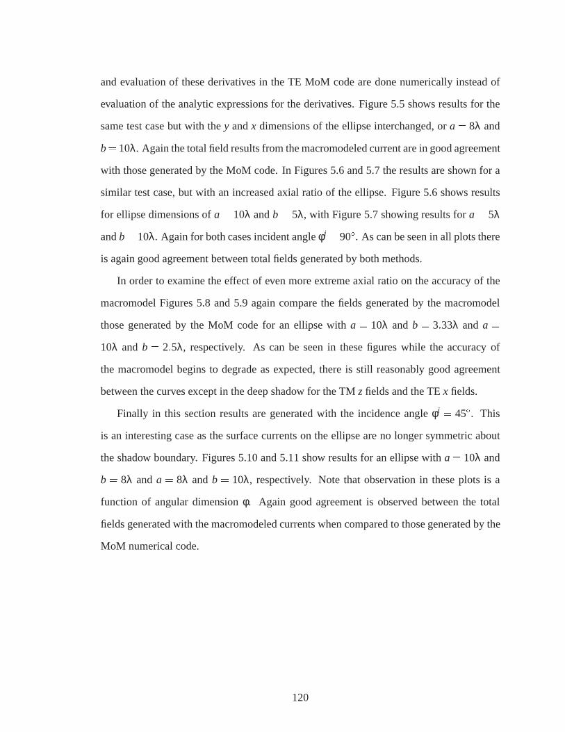
and evaluation of these derivatives in the TE MoM code are done numerically instead of
evaluation of the analytic expressions for the derivatives. Figure 5.5 shows results for the
same test case but with they andx dimensions of the ellipse interchanged, ora= 8λ and
b= 10λ. Again the total field results from the macromodeled current are in good agreement
with those generated by the MoM code. In Figures 5.6 and 5.7 the results are shown for a
similar test case, but with an increased axial ratio of the ellipse. Figure 5.6 shows results
for ellipse dimensions ofa= 10λ andb= 5λ, with Figure 5.7 showing results fora= 5λ
andb= 10λ. Again for both cases incident angleφi = 90Æ. As can be seen in all plots there
is again good agreement between total fields generated by both methods.
In order to examine the effect of even more extreme axial ratio on the accuracy of the
macromodel Figures 5.8 and 5.9 again compare the fields generated by the macromodel
those generated by the MoM code for an ellipse witha = 10λ and b = 3:33λ and a =
10λ and b = 2:5λ, respectively. As can be seen in these figures while the accuracy of
the macromodel begins to degrade as expected, there is still reasonably good agreement
between the curves except in the deep shadow for the TMzfields and the TEx fields.
Finally in this section results are generated with the incidence angleφi = 45Æ. This
is an interesting case as the surface currents on the ellipse are no longer symmetric about
the shadow boundary. Figures 5.10 and 5.11 show results for an ellipse witha= 10λ and
b = 8λ anda = 8λ andb = 10λ, respectively. Note that observation in these plots is a
function of angular dimensionφ. Again good agreement is observed between the total
fields generated with the macromodeled currents when compared to those generated by the
MoM numerical code.
120

−10 −5 0 5 10−70
−60
−50
−40
−30
−20
−10
0
10
y−dimension (wavelengths)
|EzT
M|
(a) jETMz j
−10 −5 0 5 10−30
−25
−20
−15
−10
−5
0
5
10
y−dimension (wavelengths)|E
xTE|
(b) jETEx j
−10 −5 0 5 10−70
−60
−50
−40
−30
−20
−10
0
10
y−dimension (wavelengths)
|EyT
E|
(c) jETEy j
Figure 5.4: Magnitude (dB), total fields 1λ off the surface of an ellipse, with y-dimensiona = 10λ, x-dimensionb = 8λ. Incidence angleφi is at 90Æ, MoM solution(———–), compared with macromodel (- -- - - -).
121

−10 −5 0 5 10−70
−60
−50
−40
−30
−20
−10
0
10
y−dimension (wavelengths)
|EzT
M|
(a) jETMz j
−10 −5 0 5 10−35
−30
−25
−20
−15
−10
−5
0
5
y−dimension (wavelengths)|E
xTE|
(b) jETEx j
−10 −5 0 5 10−70
−60
−50
−40
−30
−20
−10
0
10
y−dimension (wavelengths)
|EyT
E|
(c) jETEy j
Figure 5.5: Magnitude (dB), total fields 1λ off the surface of an ellipse, with y-dimensiona = 8λ, x-dimensionb = 10λ. Incidence angleφi is at 90Æ, MoM solution(———–), compared with macromodel (- -- - - -).
122

−10 −5 0 5 10−70
−60
−50
−40
−30
−20
−10
0
10
y−dimension (wavelengths)
|EzT
M|
(a) jETMz j
−10 −5 0 5 10−30
−25
−20
−15
−10
−5
0
5
10
y−dimension (wavelengths)|E
xTE|
(b) jETEx j
−10 −5 0 5 10−70
−60
−50
−40
−30
−20
−10
0
10
y−dimension (wavelengths)
|EyT
E|
(c) jETEy j
Figure 5.6: Magnitude (dB), total fields 1λ off the surface of an ellipse, with y-dimensiona = 10λ, x-dimensionb = 5λ. Incidence angleφi is at 90Æ, MoM solution(———–), compared with macromodel (- -- - - -).
123

−6 −4 −2 0 2 4 6−70
−60
−50
−40
−30
−20
−10
0
10
y−dimension (wavelengths)
|EzT
M|
(a) jETMz j
−6 −4 −2 0 2 4 6−35
−30
−25
−20
−15
−10
−5
0
5
10
y−dimension (wavelengths)|E
xTE|
(b) jETEx j
−6 −4 −2 0 2 4 6−70
−60
−50
−40
−30
−20
−10
0
10
y−dimension (wavelengths)
|EyT
E|
(c) jETEy j
Figure 5.7: Magnitude (dB), total fields 1λ off the surface of an ellipse, with y-dimensiona = 5λ, x-dimensionb = 10λ. Incidence angleφi is at 90Æ, MoM solution(———–), compared with macromodel (- -- - - -).
124

−15 −10 −5 0 5 10 15
−40
−30
−20
−10
0
10
y−dimension (wavelengths)
|ET
Mz
|
(a) jETMz j
−15 −10 −5 0 5 10 15−15
−10
−5
0
5
y−dimension (wavelengths)|E
TE
x|
(b) jETEx j
−15 −10 −5 0 5 10 15−70
−60
−50
−40
−30
−20
−10
0
y−dimension (wavelengths)
|ET
Ey
|
(c) jETEy j
Figure 5.8: Magnitude (dB), total fields 1λ off the surface of an ellipse, with y-dimensiona= 10λ, x-dimensionb= 3:33λ. Incidence angleφi is at 90Æ, MoM solution(———–), compared with macromodel (- -- - - -).
125

−15 −10 −5 0 5 10 15
−40
−30
−20
−10
0
10
y−dimension (wavelengths)
|ET
Mz
|
(a) jETMz j
−15 −10 −5 0 5 10 15−20
−15
−10
−5
0
5
y−dimension (wavelengths)|E
TE
x|
(b) jETEx j
−15 −10 −5 0 5 10 15−70
−60
−50
−40
−30
−20
−10
0
y−dimension (wavelengths)
|ET
Ey
|
(c) jETEy j
Figure 5.9: Magnitude (dB), total fields 1λ off the surface of an ellipse, with y-dimensiona = 10λ, x-dimensionb = 2:5λ. Incidence angleφi is at 90Æ, MoM solution(———–), compared with macromodel (- -- - - -).
126

−100 0 100 200 300−100
−80
−60
−40
−20
0
20
φs (degrees)
|EzT
M|
(a) jETMz j
−100 0 100 200 300−60
−50
−40
−30
−20
−10
0
10
φs (degrees)|E
xTE|
(b) jETEx j
−100 0 100 200 300−60
−50
−40
−30
−20
−10
0
10
φs (degrees)
|EyT
E|
(c) jETEy j
Figure 5.10: Magnitude (dB), total fields 1λ off the surface of an ellipse, with y-dimensiona = 10λ, x-dimensionb = 8λ. Incidence angleφi is at 45Æ, MoM solution(———–), compared with macromodel (- - - - - -).
127

−100 0 100 200 300−80
−60
−40
−20
0
20
φs (degrees)
|EzT
M|
(a) jETMz j
−100 0 100 200 300−50
−40
−30
−20
−10
0
10
φs (degrees)|E
xTE|
(b) jETEx j
−100 0 100 200 300−70
−60
−50
−40
−30
−20
−10
0
10
φs (degrees)
|EyT
E|
(c) jETEy j
Figure 5.11: Magnitude (dB), total fields 1λ off the surface of an ellipse, with y-dimensiona = 8λ, x-dimensionb = 10λ. Incidence angleφi is at 45Æ, MoM solution(———–), compared with macromodel (- - - - - -).
128

5.3.2 Knife-edge (Kirchhoff) Diffraction
A commonly used technique in predicting path loss from terrain obstacles is knife-edge
or Kirchhoff diffraction. Based on Huygen’s principle, the obstacle is represented by a
blocking screen and the field distribution across the resulting aperture (from the top of the
screen, vertically to infinity) integrated to produce the diffracted fields. The technique is
a 2-D method (does not account for oblique incidence) and assumes that both the source
and observation are very distant from the obstacle. It is a scalar method (does not account
for polarization effects) and cannot account for surface effects such as reflected fields or
creeping waves. Also it does not account for the impedance of the surface. Based on the
assumption that both source and observation are distant from the obstacle the following
expression, in the form of a Fresnel integral, can be derived for path loss by applying knife-
edge diffraction techniques, [49].
Path loss=
p2
2
����∞Z
�Hc
e�iπu2=2 du
����; (5.9)
where,
Hc =
�2(R0+ jyj)
λR0jyj � 2iπγ2
�1=2
ho: (5.10)
In (5.10)R0 is the horizontal distance from source to the blocking screen (perpendicular to
screen),y the horizontal distance from observation to screen,λ the free space wavelength,
γ a decay factor, representing a Gaussian field distribution across the aperture, andho the
vertical distance from observation to the top of the screen (see Figure 5.12 for geometry
details). Note thatHc in (5.9) and (5.10) is positive when observation is above the screen
and negative below. The geometry of the problem for both the convex surface and knife-
edge are shown in Figure 5.12. The convex obstacle is represented by a parabolic surface of
heighth and widthw, defined at the base of the surface (x= 0 in Figure 5.12). To minimize
129

Ei
●
x
y
Blocking Screen
Virtual Ground
Observation
x- observation convex
y- observation
w
h ho
Figure 5.12: Scattering Geometry, Knife-edge and Convex Surface
edge effects the parabolic surface is extended below a virtual ground (x< 0) and the surface
currents tapered by a cosine function below this point. For all results that follow the angle
of incidence for the convex surface isφi = 90Æ (normal to the screen, see Figure 5.2) and the
source position,Ro for the knife edge is assumed to be distant so that plane wave incidence
can be assumed. Also the weighting parameterγ in (5.10) is set at 1000λ or essentially a
uniform aperture distribution.
If the blocking obstacle is much narrower in width than height it is assumed that knife-
edge diffraction should produce somewhat acceptable results provided that the observation
point in the shadow region is distant from the actual obstacle, although since knife-edge
diffraction is scalar diffraction, it will not properly predict the location of the ringing posi-
tions in the lit regions. As the width of the obstacle is increased these results should begin
to degrade even further when compared with results from the macromodel for convex sur-
faces, especially in the deep shadow of the obstacle. This can be seen in Figures 5.13
through 5.15. To generate these results the observation position was placed aty = �51λ
(see Figure 5.12) and moved vertically fromx= 0 to x= 100λ. The height of the obstacle
was set at 50λ. Figure 5.13 shows results from the macromodel, with width of the convex
130

surface set atw= 6λ, compared with the knife-edge results (note that this width produces
a radius of curvature at the shadow boundary of approximately 1λ, the minimum radius of
curvature for which the macromodel can be assumed to be accurate). Figure 5.13a shows a
comparison of the z-component of the TM fields (total fields) with the knife-edge results,
with Figure 5.13b comparing the knife-edge results to the x-component of the TE fields. As
can be seen in Figure 5.13a, for the TM case, the knife-edge calculations produced some-
what acceptable in the lit region and through the transition region (again without properly
predicting the position of the ringing in the lit region) for this case of a very narrow obsta-
cle, although its accuracy begins to degrade in the deep shadow region as expected. The
results for the TE case, in Figure 5.13b, shows similar discrepancies. Figure 5.14 and
Figure 5.15 show similar results, with the width of the obstacle widened to 50 and 100λ
respectively. As expected the knife-edge results begin to degrade in the shadow region as
the width of the obstacle is increased, and the degradation tends to approach the transition
region and shadow boundary.
0 20 40 60 80 100−40
−30
−20
−10
0
10
x (wavelengths)
Pat
h lo
ss (
dB)
(a) jETMz j
0 20 40 60 80 100−40
−30
−20
−10
0
10
x (wavelengths)
Pat
h lo
ss (
dB)
(b) jETEx j
Figure 5.13: Path loss (dB), total fields from an obstacle of heighth = 50λ, and widthw= 6λ. Observation is aty=�51λ and incident angle is atφi = 90Æ (normalto the screen). Macromodel (———–), compared with knife-edge (Kirchhoff)diffraction (- - - - - -).
131
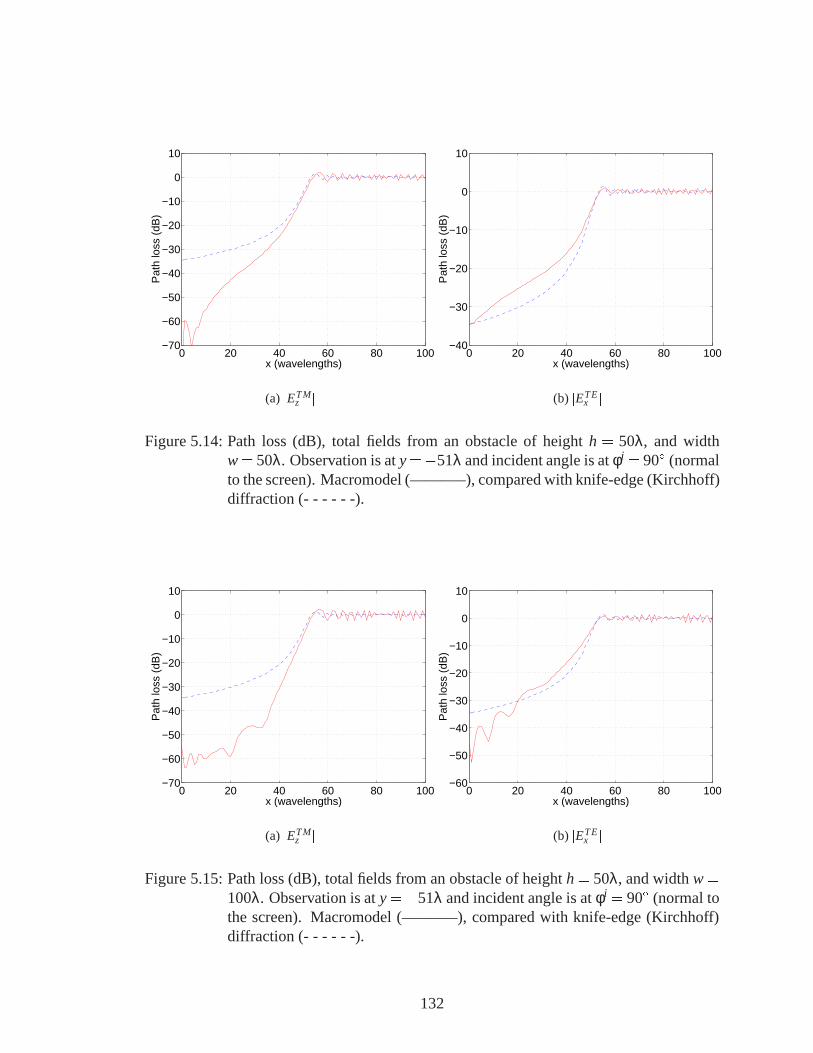
0 20 40 60 80 100−70
−60
−50
−40
−30
−20
−10
0
10
x (wavelengths)
Pat
h lo
ss (
dB)
(a) jETMz j
0 20 40 60 80 100−40
−30
−20
−10
0
10
x (wavelengths)
Pat
h lo
ss (
dB)
(b) jETEx j
Figure 5.14: Path loss (dB), total fields from an obstacle of heighth = 50λ, and widthw= 50λ. Observation is aty=�51λ and incident angle is atφi = 90Æ (normalto the screen). Macromodel (———–), compared with knife-edge (Kirchhoff)diffraction (- - - - - -).
0 20 40 60 80 100−70
−60
−50
−40
−30
−20
−10
0
10
x (wavelengths)
Pat
h lo
ss (
dB)
(a) jETMz j
0 20 40 60 80 100−60
−50
−40
−30
−20
−10
0
10
x (wavelengths)
Pat
h lo
ss (
dB)
(b) jETEx j
Figure 5.15: Path loss (dB), total fields from an obstacle of heighth= 50λ, and widthw=100λ. Observation is aty=�51λ and incident angle is atφi = 90Æ (normal tothe screen). Macromodel (———–), compared with knife-edge (Kirchhoff)diffraction (- - - - - -).
132

5.4 Chapter Summary: Diffraction from Convex Surfaces
In this chapter the macromodel developed in Chapter 4, for predicting the induced sur-
face currents on a right circular PEC cylinder, when excited by a plane wave at oblique
angles, was extended to the case of a general convex surface. Recognizing that the induced
surface currents on a circular cylinder can be applied locally on a surface with large, slowly
varying radius of curvature, the method was extended to a general convex surface by appli-
cation of standard methods found in the literature. The case of an elliptical cylinder was first
examined and the proposed macromodel showed good agreement when compared to results
generated by a MoM numerical code. The macromodel was then applied to a parabolic sur-
face and compared to results generated by using knife-edge or Kirchhoff diffraction. As
expected the knife-edge method produced somewhat acceptable results for a very narrow
obstacle, but as the obstacle was widened, results from the knife-edge method began to
degrade, especially in the shadow region and into the transition region.
133

CHAPTER 6
Summary & Future Work
As previously discussed, the ability to predict the propagation of radio waves in an ac-
curate and general fashion is essential in the performance analysis and optimal design of
a communications system. Without an accurate and general model, system issues such as
coherency, field variations, multipath, and path delay effects cannot be properly addressed.
Existing methods in propagation or channel modeling tend to be heuristic or overly sim-
plistic and do not adequately address the relevant issues for optimal system design. Due
to the discussed shortcomings in current techniques for the prediction of radio wave prop-
agation, a more general approach or methodology, directly based on the physics of the
propagation problem is defined. The basis of the methodology is, through the application
of electromagnetic wave theory, to develop a series of canonical scattering and diffraction
models which represent the effects of various mechanisms in the propagation environment,
on the radio wave. Depending on the problem at hand the appropriate technique is applied
whether it be analytic, numeric, or a hybrid technique. Relevant approximations are made,
based on the physics of the problem, which improve computational efficiency while re-
taining the required accuracy. Eventual merger of these canonical models with a satellite
terrain database will provide the system designer with an accurate and general model to
simulate the propagation environment.
Within the framework of this physics-based methodology the initial concentration or
134

focus of this thesis work was defined. It is intended that the work in this thesis be a basis
for expansion into an overall propagation model, and with that in mind it was decided that
the concentration of this work would be on predicting propagation in a rural environment,
in the frequency range of HF to L-band, which can include point to point communication
on the ground or perhaps from an unmanned aerial vehicle (UAV) to/from ground. Included
in a rural environment can be the effects of a lossy earth on radio wave propagation as well
as scattering and diffraction from natural obstacles such as hills, mountains, or ridgelines.
In this thesis two diffraction models were developed. The first accounts for the effects of
a lossy earth on the fields of a small dipole, which can include the effects of some type of
impedance transition, representative of a river or land/sea transition. The second model de-
veloped determines scattering and diffraction from a general convex surface, representative
of a hill, mountain, or ridgeline. In this chapter this work will be summarized as well as a
discussion of future work presented.
6.1 Summary: Scattering & Diffraction from Impedance
Surfaces
The prediction of radio wave propagation over the Earth’s surface is important in the
characterization of a communications channel. Locally the Earth can be modeled as a flat,
impenetrable, impedance surface and the standard impedance boundary condition (SIBC)
applied. The problem can be decomposed into the effects of the homogeneous surface and
the effects of an impedance transition in the surface, such as caused by a river or land/sea
interface. In Chapter 2 the effects of the homogeneous surface were addressed with the
model extended to include that of an impedance transition in Chapter 3.
135
6.1.1 Fields of a Small Dipole Above an Impedance Surface
The fields of an infinitesimal dipole, of arbitrary orientation, above a homogeneous
impedance surface is the classic Sommerfeld problem, with field expressions in the form
of Sommerfeld type integrals. These integrals are highly oscillatory and difficult to evaluate
numerically and the time taken to compute them discourages their application as Green’s
functions in integral equation techniques. With this in mind, in Chapter 2, a technique was
presented to significantly improve the convergence properties of these Sommerfeld type
integrals. By application of an integral transform technique known as exact image theory
the Sommerfeld type integrals were transformed into a form more conducive to numeri-
cal evaluation. As no approximations are made the resulting expressions are exact in the
analytic sense. Starting with a spectral domain representation of the dipole fields, and by
application of appropriate identities, the expressions are modified to consist of Bessel func-
tions of the first kind, of order zero, only. Reflection coefficients are then cast in the form
of the Laplace transform of an exponential function. The spectral domain integration can
then be performed analytically and the remaining integrals in the Laplace domain converge
extremely rapidly, up to several orders of magnitude faster than the original Sommerfeld
type expressions. Expressions for a horizontal dipole show a diverging exponential term
not previously discussed in the literature. The integrand for this case however, is still domi-
nated by a decaying exponential term and the rapid convergence properties are maintained.
6.1.2 Scattering from an Impedance Transition
Having developed a technique for efficient calculation of the fields of a dipole above
a homogeneous impedance surface, the model, in Chapter 3, was extended to include the
effects of a one-dimensional impedance transition in the surface, which can represent the
effects of a river or land/sea transition. Current methods in use, such as the Geometrical
Theory of Diffraction (GTD), are only valid for an abrupt transition and a method was
136

sought which is valid for any arbitrary, one-dimensional, impedance transition function. A
perturbation technique is applied in which the impedance transition is represented as a per-
turbation in the surrounding impedance half-space. An integral equation is defined on the
impedance surface and the unknown surface currents in the resulting expression expanded
in terms of a perturbation parameter. For ease of analysis the resulting expressions are
solved in the Fourier domain for the unknown surface currents and recursive expressions
are obtained, relating higher order currents in the perturbation series to lower order in the
form of multi-fold convolution. An error bound was established which shows the perturba-
tion series to converge for a lossy surface, even for a very large perturbation parameter. All
field integrals were solved by application of stationary phase techniques producing field
expressions which are algebraic to first order in the perturbation series.
The technique was than applied to calculate the scattering effects of a land/sea transi-
tion on the total dipole fields. For this problem the impedance transition function was dealt
with in a mean sense, i.e., the unperturbed impedance (homogeneous surface) is the mean
value of the transition function. The perturbation technique inherently deals with the unper-
turbed impedance in this way and the assumption of a mean impedance is valid for source
and observation near the impedance surface, the case of interest to us. In this case the Ge-
ometrical Optics (GO) and direct fields tend to cancel and higher order terms dominate the
total dipole fields (Norton surface wave). The fields scattered from the impedance transi-
tion are now comparable to those from the homogeneous surface and thus it was shown that
the transition has a significant effect even distant from the land/sea interface. For this same
case, and when source and observation are also distant from each other, the observation is
near grazing and tends to be near the specular direction. Analysis presented shows that the
effects of the width of the land/sea transition are negligible in the specular direction and
thus the transition width has no effect on the fields when source and observation are near
the impedance surface. It was also shown in Chapter 3 that an apparent discontinuity in
the total fields at the GO reflection boundary was an artifact of applying stationary phase
137

to determine the dominate spectral component or plane wave of the dipole fields which ex-
cites the transition. This single plane wave contains infinite energy across the extent of the
impedance surface and therefore the Fourier transform of the impedance transition function
contains infinite energy. Analysis showed that while the field levels through the reflection
boundary are not discontinuous they do transition very rapidly and the fields on each side
of the reflection boundary are correct.
6.2 Summary: Diffraction from Convex Surfaces
In a rural environment natural obstacles such as hills, mountains, or ridgelines can ex-
hibit the features of a long, slowly varying curved surface, which is essentially infinite in
one-dimension and can have a significant effect on radio wave propagation. Even at HF
frequencies these obstacles exhibit a finite radius of curvature which must be accounted
for, and currently applied techniques such as knife-edge (Kirchhoff) diffraction and wedge
diffraction do not address this. To address the issue of diffraction from convex surfaces high
frequency techniques are the appropriate tool, however as was shown they are mathemat-
ically complex, and can be highly inaccurate (Uniform Theory of Diffraction (UTD)). As
no one high frequency technique is valid in all regions around the obstacle it was decided
to work with the induced surface currents, which through the radiation integrals produce
fields in all regions. For surfaces with large, slowly varying radii of curvature, the cur-
rents excited on a circular cylinder are a valid approximation to those induced on a general
convex surface. While the Fock integrals can be used to calculate these induced surface
currents they were shown to be numerically cumbersome and in fact impractical for calcu-
lating the currents on cylinders of even moderate radius. With this as a motivation a novel
technique was introduced and developed in Chapter 4 to approximate the currents induced
on the surface of a PEC right circular cylinder, when excited by a plane wave.
The induced surface currents on a cylinder can be decomposed, in the manner of the
138

Physical Theory of Diffraction (PTD), into a uniform or Physical Optics (PO) component
and a non-uniform or diffraction component which is a correction to the PO currents. The
PO currents are a form of the incident field and are know, thus the objective is to determine
a model for the diffraction currents. In Chapter 4 a macromodel for the diffraction currents
is developed which is simple, yet highly accurate and requires no numerical integration.
Based on Fock analysis, the high frequency behavior of the induced surface currents, as
a function of cylinder radius, is predicted. As shown in Chapter 4 this in practice means
applying simple scaling and weighting factors to the induced surface currents for a cylinder
of moderate radius in order to generate the surface currents for cylinders of any radius above
one wavelength. The resulting currents produce total fields with a dynamic range of over
85 dB.
In Chapter 5 the induced surface currents from the right circular cylinder were applied
locally, in a standard fashion to approximate the currents induced on a general convex
surface. To validate the method on a non-circular cylinder results were first generated for an
elliptical cylinder using the macromodeled currents and compared to those generated with
a Method of Moments (MoM) code, showing good agreement for all cases. Results from
the macromodel when applied to a parabolic surface were then generated and compared
to results from knife-edge diffraction. As expected the knife-edge results degraded in the
shadow region and as the parabolic surface became less narrow in width.
6.3 Future Work
The propagation problem is an open ended one and it is an understatement to say that
there is still a significant amount of research to be pursued. There are several things that
still need to be addressed in further development of the models described in this thesis and
that will be discussed in the sections that follow. It it appropriate beforehand however to
discuss recommendations for future work in terms of the overall context of the propagation
139

problem. Having developed a basis for an overall propagation model both in this thesis and
in the work of other students involved in the project the next logical step in the process
is to address the issues of integration of the canonical geometries into a coherent propa-
gation model, including the statistical nature of the propagation environment and relevant
interactions between the individual models. A parallel effort should include the integra-
tion of a remote sensing satellite data base to model the physical environment within the
overall propagation scenario. Currently available remote sensing databases include all rel-
evant parameters including the topography of the terrain (digital elevation maps (DEM))
as well as statistical variations of the propagation environment such as soil moisture, snow
cover, vegetation classification, etc. In addition an obvious step would be the investigation
and application of these diffraction and scattering models to an urban environment. The
urban environment is of significant interest in the prediction of propagation for mobile sys-
tems and no techniques developed to date address the relevant issues inherent in an urban
environment. Finally and as should be obvious validation of the propagation model by
comparison with measured data should be pursued.
6.3.1 Future Work: Fields of a Dipole Above an Impedance Surface
To complete the model for the fields of a small dipole above an impedance surface
several issues can be investigated. The current model applies stationary phase techniques
to evaluate the field integrals and because of this approximation the dipole must be dis-
tant from the impedance transition. A more rigorous evaluation of the field integrals can
be examined which allows arbitrary placement of both the dipole and observation, while
maintaining the computational efficiency required. The perturbation method applied to cal-
culate scattering from a general impedance transition can determine the scattered fields for
any transition for which the Fourier transform exists. As an additional investigation other
types of transitions can be investigated including a swamp/dry land transition or a small
trough or depression in the terrain.
140

6.3.2 Future Work: Diffraction From Convex Surfaces
The macromodel developed in Chapters 4 and 5 is for the case of a PEC surface when
excited by a plane wave and is intended to serve as a basis for determining the effects of
natural obstacles on radio wave propagation. There are two obvious extensions to the work
that must be developed in order to make the model of practical use. The first is to extend
the model to include dipole excitation. An initial step in this extension could be to restrict
the dipole location to be distant from the obstacle and thus only one spectral component of
the dipole expansion need be accounted for. The second is to extend the macromodel to
the case of a general impedance surface. As a significant amount of time was invested into
investigating this problem, some further discussion is in order.
It was initially believe that the macromodel for a PEC cylinder could be extended to that
of an impedance cylinder in a simple fashion by assuming that the currents on an impedance
cylinder could be represented as a perturbation from the PEC case. For the TM case this
assumption in fact proved to be true. If each term of the eigenseries for an impedance
cylinder is expanded into a Taylor series, for which the lowest order term represents the
PEC case it is observed that the convergence properties of the Taylor series improve as
cylinder radius increases. If the limiting case of an cylinder of infinite radius is examined
and the expressions for the induced surface currents similarly expanded into a Taylor series,
it can be shown that the series will always converge, for the TM case. A similar analysis
of the eigenseries for the TE case however shows a degradation in the convergence of the
the embedded Taylor series for increasing cylinder radius. Again looking at the limiting
case of a cylinder of infinite radius it can be shown that, for the TE case, the Taylor series
expansion will never converge for incident angles beyond Brewster’s angle. This analysis
indicates that in fact the approach of representing the impedance currents as a perturbation
from the PEC currents is not a valid one and alternate approaches need be investigated.
141

APPENDICES
142

Appendix A
Alternate Spectral Domain Representation the Fields of a
Small Dipole Above an Impedance Half-Space
In this appendix an alternate spectral domain representation for the electric fields of an
infinitesimal electric dipole radiating above a homogeneous, infinite impedance half-space
is derived. The geometry of the problem is as shown in Figure A.1. Starting with the the
standard spectral domain representation for the fields of a dipole above an impedance half-
space (Green’s function) an appropriate change of variables is then applied. Application of
Bessel identities will result in the final form of the spectral domain representation of the
dipole fields.
The standard spectral representation for the fields of a small dipole above an impedance
half-space (Green’s function), of lengthl , orientationl and carrying currentI0, is given by
143

●
Z1
φ
D
-z
z
z
x
y
Observation
R
θ
k ,Z 00
I l0
0
0
0
Figure A.1: Problem geometry, dipole above an impedance plane
[34],
ET(r ; r0) =� iI0Z0lk0
(l � z)z δ(r � r0)
�
8>>>>>>>>>>>>>>>>>>>>>>><>>>>>>>>>>>>>>>>>>>>>>>:
k0Z0I0l8π2
+∞RR�∞
dkx dkyei(kx(x�x0)+ky(y�y0))
kz
fh(kz) [Γh(h(kz) � l) eikzz0 +(h(kz) � l) e�ikzz0]
+ v(kz) [Γv(v(�kz) � l) eikzz0 +(v(kz) � l) e�ikzz0]g eikzz for z > z0
k0Z0I0l8π2
+∞RR�∞
dkx dkyei(kx(x�x0)+ky(y�y0))
kz
f[h(kz)Γh eikzz+ h(kz) e�ikzz] (h(kz) � l)
+ [v(kz)Γv eikzz+ v(�kz) e�ikzz](v(�kz) � l)g eikzz0 for 0 < z< z0:
(A.1)
In (A.1) k = kxx+kyy+kzzwith dependent variable,kz defined askz =q
k20�k2
x�k2y, and
144
the branch cut defined asi =p�1. The polarization unit vectorsh andv are given by
h(kz) =k� zjk� zj ; v(kz) =
h(kz)�kk0
; (A.2)
and,
h(�kz) =K � zjK � zj ; v(�kz) =
h(�kz)�Kk0
; (A.3)
where h indicates horizontal polarization (transverse electric (TE) toz) and v indicates
vertical polarization (transverse magnetic (TM) toz), andK = k�2(k � z)z= kxx+ kyy�kzz. The reflection coefficientsΓh and Γv (horizontal and vertical reflection coefficients
respectively) in (A.1) are defined as,
Γh =η�k0=kz
η+k0=kz; Γv =
�η+kz=k0
η+kz=k0; (A.4)
whereη is the normalized surface impedance,η = Z1=Z0. The terms containingΓh andΓv
in (A.1) represent the effects of the impedance surface on the total field and are designated
as the diffracted fields, with the the other terms representing the direct dipole fields. The
direct dipole electric fields are more convieniently evaluated in the spatial domain and are
given in dyadic form by
Eid(r ; r0) =
�ik0Z0I0l4π
�I +
1
k20
∇∇�
eik0jr�r0j
4π� l ; (A.5)
wherer =p
x2+y2+z2 is the distance to the observation point andr0 =p
x02+y0
2+z02
is the distance to the source location. Expanding (A.5) gives the more useful form of the
145
direct dipole fields or
Ei(r ; r0) = ik0Z0I0l
��3
k20R2
0
� 3ik0R0
�1
�R0(l � R0)
+
�1+
ik0R0
� 1
k20R2
0
�l
�eik0R0
4πR0;
(A.6)
whereR0 = jr � r0j=p
(x�x0)2+(y�y0)2+(z�z0)2 andR0 =r�r0jr�r0j
.
To derive an alternate representation for the diffracted dipole fields in the spectral do-
main, the standard change of variables is first applied to (A.1),
kx = kρ cosν; x�x0 = Dcosφ;
ky = kρ sinν; y�y0 = Dsinφ;(A.7)
resulting in the following expression for the diffracted dipole fields,
Ed(r ; r0) =k0Z0I0l
8π2
2πZ
0
∞Z
0
kρ
kz[Γh(h� l)h+Γv(v(�kz) � l)v(kz)]
eikz(z+z0)eikρDcos(ν�φ) dν dkρ; (A.8)
In (A.8), (h � l)h and(v(�kz) � l)v(kz) can be rewritten in terms of the new variables as
(h� l)h= (lxsin2ν� lysinνcosν)x+(�lxsinνcosν+ lycos2 ν)y; (A.9)
and
(v(�kz) � l)v(kz) =1
k20
f�kzcosν[kρlz+kz(lxcosν+ lysinν]x
�kzsinν[kρlz+kz(lxcosν+ lysinν)]y
+kρ[kρlz+kz(lxcosν+ lysinν)]zg:
(A.10)
Substituting (A.9) and (A.10) into (A.8) and recognizing that cos2 ν = (1+ cos2ν)=2,
sin2ν = (1� cos2ν)=2, and sinνcosν = (1=2)sin2ν and by applying the following two
146
identities
2πZ
0
cos(nν) eikρDcos(ν�φ) dν = 2π(i)ncos(nφ) Jn(kρD); (A.11)
2πZ
0
sin(nν) eikρDcos(ν�φ) dν = 2π(i)nsin(nφ) Jn(kρD): (A.12)
the diffracted electric fields in (A.8) can be rewritten as
Ed(r ; r0) =k0Z0I0l
4π
�x
∞Z
0
kρ
2kzfΓh[�lx(J2(kρD)cos2φ+J0(kρD))� lyJ2(kρD)sin2φ)]
+Γv[2ikzkρ
k20
lzcosφJ1(kρD)+k2
z
k20
lx(J0(kρD)�J2(kρD)cos2φ)
�k2z
k20
lyJ2(kρD)sin2φ]g eikz(z+z0) dkρ
+y
∞Z
0
kρ
2kzfΓh[�lxJ2(kρD)sin2φ� ly(J0(kρD)�J2(kρD)cos2φ)]
+Γv[2ikzkρ
k20
lzsinφJ1(kρD)� k2z
k20
lxJ2(kρD)sin2φ
+k2
z
k20
ly(J0(kρD)+J2(kρD)cos2φ)]g eikz(z+z0) dkρ
�z
∞Z
0
kρ
kzΓv[
k2ρ
k20
lzJ0(kρD)+ikzkρ
k20
(lxcosφ
+lysinφ)J1(kρD)] eikz(z+z0) dkρ
�;
(A.13)
(A.13) is an alternate spectral domain representation for the fields of a small dipole above
an impedance half-space and the integrals contained within are Sommerfeld type integrals.
147

Appendix B
Derivation of 2-D Dyadic Green’s Function
In this appendix the spectral representation of the 2-D dyadic Green’s function will be
derived. The geometry of the problem is as shown in Figure B.1. Observe thatθ andφ
are defined as in standard spherical coordinates with angleβ defined from the ˆy axis and is
used for projection into the ˆx� z plane. Note that the geometry is not a function of ˆy and
thus the induced current along ˆy, and the scattered field, are of the form,ekiyy or are in phase
with the incident field. The incident field vectork i is defined as,
k i = kixx+ki
yy+kizz (B.1)
where,kix = k0sinθi cosφi , ki
y = k0sinθi sinφi , andkiz = k0cosθi.
First we start with the free space dyadic Green’s function which has the following form
in the spectral domain,
G(r ; r 0) =� zzδ(r� r 0)
k20
+
8>><>>:
i8π2
RR 1kz[I � kk
k20] ei(kx(x�x0)+ky(y�y0)+kz(z�z0)) dkx dky for z > z0;
i8π2
RR 1kz[I � KK
k20] ei(kx(x�x0)+ky(y�y0)�kz(z�z0)) dkx dky for z < z0;
(B.2)
whereK = k�2(k � z)z.
148

x
yz
θ i
ϕi
ψEi
Specular Cone
β
β
Es
Z(x)
Figure B.1: Scattering geometry for variable impedance surface.
Since the dependence of the induced currents and fields ony is known (eikiyy), the 2-D
Green’s function can evaluated from (B.2) by integrating out they dimension to arrive at,
G2D(ρ;ρ0) = �zzδ(ρ�ρ0)
k20
eikiyy
+eikiyy
8>><>>:
i4π
R 1kz[I � kk] ei(kx(x�x0)+kz(z�z0)) dkx for z > z0;
i4π
R 1kz[I � KK] ei(kx(x�x0)�kz(z�z0)) dkx for z < z0;
(B.3)
whereρ = xx+zzandkz =q
k20�ki
y2�k2
x =q
k20 sin2 β�k2
x. Hereβ is defined byki � y=cosβ = sinθi sinφi .
Noting that[I� kk] = ee+mm, the 2-D Green’s function in the spectral domain is given
in its final form by
G2D?(ρ;ρ0) = eikiyy i
4π
Z1kz
[ee+ mm] ei(kx(x�x0)+kz(z�z0)) dkx; (B.4)
whereeandm correspond to the TE and TM cases, respectively, and are given by
e= k� y and m= e� k: (B.5)
149

Noting that,k= [kxx+kyy+kzz]=k0, simplified expressions for ˆeandm are given by,
e=kxz�kzxk0sinβ
and m=y�cosβ k
sinβ: (B.6)
150

BIBLIOGRAPHY
151
BIBLIOGRAPHY
[1] J. E. Hipp, “Soil Electromagnetic Parameters as Functions of Frequency, Soil Density,and Soil Moisture,” Proceedings of the IEEE, vol. 62, no. 1, pp. 98–103, January1974.
[2] Y. Okumura, E. Ohmori, T. Kawano, and K. Fukuda, “Field Strength and its Variabil-ity in VHF and UHF Land Mobile Service,”Rev. Elec. Comm. Lab, vol. 16, pp. 825,September-October 1968.
[3] A. G. Longley and P. L. Rice, “Prediction of Tropospheric Radio Transmission LossOver Irregular Terrain, A Computer Method - 1968,” Tech. Rep. ERL79-ITS67,ESSA Research Laboratories, Washington, D.C., 1968, US Government Printing Of-fice.
[4] T. B. A. Senior, and J. L. Volakis,Approximate Boundary Conditions in Electromag-netics, IEE Press, London, 1995.
[5] F. T. Ulaby, R. K. Moore, and A. K. Fung,Microwave Remote Sensing, Active andPassive, Vols. I, II, and III, Artech House, Norwood, MA, 1986.
[6] P. Y. Ufimtsev, “Method of Edge Waves in the Physical Theory of Diffraction,” Tech.Rep. Engl. transl. available from Nat. Tech. Inform. Serv., Springfield, VA 22161 ;#AD733203, Sovyetskoye Radio, Moscow, Russia, 1962.
[7] A. Sommerfeld, “Uber die Ausbreitung der Wellen in der drahtlosen Telegraphie,”Ann. Physik, vol. 28, pp. 665–736, 1909.
[8] H. Weyl, “Ausbreitung elektromagnetischer wellen ¨uber einem ebenen Leiter,”Ann.Physik, vol. 60, pp. 481–500, 1919.
[9] A. Sommerfeld, “Uber die Ausbreitung der Wellen in der drahtlosen Telegraphie,”Ann. Physik, vol. 81, pp. 1135–1153, 1926.
[10] B. van der Pol and K. F. Niessen, “Uber die Ausbreitung elektromagnetischer Wellenuber eine ebene Erde,”Ann. Physik, vol. 6, pp. 273–294, 1930.
[11] W. H. Wise, “The Grounded Condenser Antenna Radiation Formula,”Proceedingsof the I.R.E., vol. 19, pp. 1684–1689, September 1931.
152

[12] K. A. Norton, “The Propagation of Radio Waves over the Surface of the Earth andin the Upper Atmosphere: Part I,”Proceedings of the I.R.E., vol. 24, no. 10, pp.1367–1387, October 1936.
[13] K. A. Norton, “The Propagation of Radio Waves over the Surface of the Earth andin the Upper Atmosphere: Part II,”Proceedings of the I.R.E., vol. 25, no. 9, pp.1203–1236, September 1937.
[14] A. Banos,Dipole Radiation in the Presence of a Conducting Half-Space, Pergamon,Oxford, 1966.
[15] L. B. Felsen and N. Marcuvitz,Radiation and Scattering of Waves, IEEE Press,Piscataway, NJ, 1994.
[16] J. R. Wait,Electromagnetic Waves in Stratified Media, IEEE Press, New York, 1996.
[17] P. Parhami, Y. Rahmat-Samii, and R. Mittra, “An Efficient Approach for EvaluatingSommerfeld Integrals Encountered in the Problem of a Current Element Radiatingover Lossy Ground,”IEEE Trans. Antennas Propagat., vol. 28, no. 1, pp. 100–104,January 1980.
[18] K. A. Michalski, “On the Efficient Evaluation of Integrals Arising in the SommerfeldHalf-space Problem,”IEE Proceedings, Part H-Microwave, Antennas and Propagat.,vol. 132, no. 5, pp. 312–318, August 1985.
[19] W. A. Johnson and D. G. Dudley, “Real Axis Integration of Sommerfeld Integrals:Source and Observation Points in Air,”Radio Sci., vol. 18, no. 2, pp. 313–324, March-April 1983.
[20] H. G. Booker and P. C. Clemmow, “A Relation Between the Sommerfeld Theory ofRadio Wave Propagation Over a Flat Earth and the Theory of Diffraction at a StraightEdge,” IEE Proceedings, vol. 97, Part III, no. 45, pp. 18–27, January 1950.
[21] B. van der Pol, “Theory of the Reflection of the Light from a Point Source by aFinitely Conducting Flat Mirror: With an Application to Radiotelegraphy,”Physica,vol. 2, pp. 843–853, 1935.
[22] K. Furutsu, “On the Excitation of the Waves of Proper Solutions,”I.R.E. Trans.Antennas Propagat., vol. 7, Special Supplement, pp. 209–218, 1959.
[23] I. V. Lindell and E. Alanen, “Exact Image Theory for the Sommerfeld Half-SpaceProblem, Part I: Vertical Magnetic Dipole,”IEEE Trans. Antennas Propagat., vol. 32,no. 2, pp. 126–133, February 1984.
[24] I. V. Lindell and E. Alanen, “Exact Image Theory for the Sommerfeld Half-SpaceProblem, Part II: Vertical Electric Dipole,”IEEE Trans. Antennas Propagat., vol. 32,no. 8, pp. 841–847, August 1984.
153
[25] I. V. Lindell and E. Alanen, “Exact Image Theory for the Sommerfeld Half-SpaceProblem, Part III: General Formulation,”IEEE Trans. Antennas Propagat., vol. 32,no. 10, pp. 1027–1032, October 1984.
[26] P. C. Clemmow, “Radio Wave Propagation Over a Flat Earth Across a BoundarySeparating Two Different Media,”Phil. Trans. Roy. Soc. London, vol. 246-A, pp.1–55, 1953.
[27] G. D. Maliuzhinets, “Excitation, Reflection, and Emission of Surface Waves from aWedge with Given Face Impedances,”Soviet Phys. Dokl., vol. 3, pp. 752–755, 1958.
[28] J. Bazer and S. N. Karp, “Propagation of Plane Electromagnetic Waves Past a Shore-line,” J. Res. (Natl. Bur. Std.), vol. D66, pp. 319–334, 1962.
[29] J. R. Wait, “Recent Analytical Investigations of Electromagnetic Ground Wave Prop-agation over Inhomogeneous Earth Models,”Proceedings of the IEEE, vol. 62, no. 8,pp. 1061–1072, August 1974.
[30] G. de Jong, “Electromagnetic Wave Propagation over an Inhomogeneous Flat Earth(Two-Dimensional Integral Equation Formulation),”Radio Sci., vol. 10, no. 11, pp.925–933, November 1975.
[31] R. H. Ott, “RING: An Integral Equation Algorithm for HF-VHF Radio Wave Prop-agation over Irregular, Inhomogeneous Terrain,”Radio Sci., vol. 27, no. 6, pp. 867–882, November-December 1992.
[32] K. Sarabandi, “Scattering from Variable Resistive and Impedance Sheets,”Journalof Electromagnetic Waves and Applications, vol. 4, no. 9, pp. 865–891, 1990.
[33] M. I. Herman and J. L. Volakis, “High Frequency Scattering from PolygonalImpedance Cylinders and Strips,”IEEE Trans. Antennas Propagat., vol. 36, pp. 679–688, 1988.
[34] J. A. Kong,Electromagnetic Wave Theory, J. W. Wiley & Sons, New York, 1990.
[35] J. D. Murray,Asymptotic Analysis, Springer-Verlag, New York, 1984.
[36] V. A. Borovikov, Uniform Stationary Phase Method, The Institution of ElectricalEngineers, London, 1994.
[37] P. C. Clemmow, “Some Extensions to the Method of Integration by Steepest De-scents,”Quart. Journ. Mech. and Applied Math., vol. III, Pt. 2, pp. 241–256, 1950.
[38] J. Boersma and Y. Rahmat-Samii, “Comparison of Two Leading Uniform Theoriesof Edge Diffraction with the Exact Uniform Asymptotic Solution,”Radio Sci., vol.15, no. 6, pp. 1179–1194, November-December 1980.
[39] R. J. Luebbers, “Finite Conductivity Uniform GTD Versus Knife Edge Diffraction inPrediction of Propagation Path Loss,”IEEE Trans. Antennas Propagat., vol. 32, no.1, pp. 70–76, January 1984.
154

[40] C. A. Balanis, Advanced Engineering Electromagnetics, J. W. Wiley & Sons, NewYork, 1989.
[41] J. J. Bowman, T. B. A. Senior, and P. L. E. Uslenghi,Electromagnetic and AcousticScattering by Simple Shapes, Hemisphere, New York, 1969.
[42] J. B. Keller, “Diffraction by a Convex Cylinder,”I.R.E. Trans. Antennas Propagat.,vol. 4, no. 3, pp. 312–321, July 1956.
[43] P. H. Pathak, “An Asymptotic Analysis of the Scattering of Plane Waves by a SmoothConvex Cylinder,”Radio Sci., vol. 14, no. 3, pp. 419–435, May-June 1979.
[44] P. Hussar and R. Albus, “On the Asymptotic Frequency Behavior of Uniform GTD inthe Shadow Region of a Smooth Convex Surface,”IEEE Trans. Antennas Propagat.,vol. 39, no. 12, pp. 1672–1680, December 1991.
[45] V. A. Fock, “The Field of a Plane Wave Near the Surface of a Conducting Body,”J.Phys. USSR., vol. X, no. 5, pp. 399–409, 1946.
[46] L. W. Pearson, “A Scheme for Automatic Computation of Fock-type Integrals,”IEEETrans. Antennas Propagat., vol. 35, no. 10, pp. 1111–1118, October 1987.
[47] N. A. Logan, “General Research in Diffraction Theory, Vols. 1 & 2,” Tech. Rep.LMSD-288088 & 288089, Lockheed Missiles and Space Division, Sunnyvale, CA,1959.
[48] R. F. Harrington,Time-Harmonic Electromagnetic Fields, McGraw-Hill, New York,1961.
[49] R. E. Collin,Antennas and Radiowave Propagation, McGraw-Hill, New York, 1985.
155