rotational-vibrational resonance states

Rotational-vibrational resonance states

Journal: Physical Chemistry Chemical Physics

Manuscript ID CP-PER-02-2020-000960.R1

Article Type: Perspective

Date Submitted by the Author: 24-Apr-2020

Complete List of Authors: Csaszar, Attila; Eötvös Loránd Tudományegyetem, Institute of Chemistry; MTA-ELTE Complex Chemical Systems Research GroupSimko, Iren; Eötvös Loránd Tudományegyetem, Institute of ChemistrySzidarovszky, Tamás; Eötvös Loránd Tudományegyetem, Chemistry; MTA-ELTE Complex Chemical Systems Research GroupGroenenboom, Gerrit; University of Nijmegen, Theoretical Chemistry, IMMKarman, Tijs; Harvard-Smithsonian Center for Astrophysics ITAMP, Center fo Astrophysicsvan der Avoird, Ad; Institute of theoretical chemistry

Physical Chemistry Chemical Physics

Journal Name

Rotational-vibrational resonance states

Attila G. Császár,∗a,b Irén Simkób, Tamás Szidarovszky∗b,c, Gerrit C. Groenenboomd ,Tijs Karmane, and Ad van der Avoird∗d

Resonance states are characterized by an energy that is above the lowest dissociation thresholdof the potential energy hypersurface of the system and thus resonances have finite lifetimes. Allmolecules possess a large number of long- and short-lived resonance (quasibound) states. A con-siderable number of rotational-vibrational resonance states are accessible not only via quantum-chemical computations but also by spectroscopic and scattering experiments. In a number ofchemical applications, most prominently in spectroscopy and reaction dynamics, consideration ofrotational-vibrational resonance states is becoming more and more common. There are differ-ent first-principles techniques to compute and rationalize rotational-vibrational resonance states:one can perform scattering calculations or one can arrive at rovibrational resonances using vari-ational or variational-like techniques based on methods developed for determining bound eigen-states. The latter approaches can be based either on the Hermitian (L2, square integrable) or non-Hermitian (non-L2) formalisms of quantum mechanics. This Perspective reviews the basic con-cepts related to and the relevance of shape and Feshbach-type rotational-vibrational resonancestates, discusses theoretical methods and computational tools allowing their efficient determina-tion, and shows numerical examples from the authors’ previous studies on the identification andcharacterization of rotational-vibrational resonances of polyatomic molecular systems.

1 IntroductionThe quantum phenomenon of resonances,1–6 i.e., the existenceof metastable (quasibound) states embedded in the contin-uum spectra of Hamiltonians, plays an important, often cru-cial role in a number of fields related to atomic and molecularphysics and chemistry. These include the process of α decay(where resonance states were perhaps first considered in 1928),1

nuclear reactions,7,8 binary elementary reactions,4,5,9–11 high-resolution molecular spectroscopy,12–14 transition-state spec-troscopy,15–17 unimolecular decomposition,18 (reactive) scatter-ing (the first scattering resonance in atoms was observed in196319),19–21 electronic,22 vibrational,23,24 and rotational25

predissociation, autoionization,26 photoionization,27 photodisso-ciation,28,29 photoassociation30 and magnetoassociation,31 con-

a MTA-ELTE Complex Chemical Systems Research Group, P.O. Box 32, H-1518 Budapest112, Hungary; E-mail: [email protected] Institute of Chemistry, ELTE Eötvös Loránd University, H-1117 Budapest, Pázmány

Péter sétány 1/A, Hungaryc MTA-ELTE Complex Chemical Systems Research Group, P.O. Box 32, H-1518 Budapest112, Hungary; E-mail: [email protected]

d Institute of Theoretical Chemistry, Institute for Molecules and Materials, Rad-boud University, Heyendaalseweg 135, 6525 AJ, Nijmegen, Netherlands; E-mail:[email protected] Center for Astrophysics, Harvard & Smithsonian, 60 Garden Street, Cambridge, MA

02138, USA

trolled cold and ultracold chemistry,32–34 and the list could beeasily continued. In this perspective we focus on the rotational-vibrational resonances of polyatomic molecules, playing a funda-mental role in chemical reactions, as well as in molecular scatter-ing and spectroscopy. Although resonance states of a system havehigher energy than a corresponding dissociation limit (most of-ten the first one, but this may not always be the case, vide infra),dissociation from these states does not happen instantaneously.

Resonance states have well-defined finite lifetimes, which canbe very short or very long, to some extent independent of theenergy of the state. One must thus emphasize that despite theirsomewhat unusual properties, resonance states are always “gen-uine”, they arise from intrinsic properties characterizing mostquantum systems. Thus, rotational-vibrational (rovibrational)resonance states should be considered neither exotic nor es-oteric,35 as both their experimental observation10,12,16,17,35–55

and first-principles characterization13,14,47,56–68 is becoming in-creasingly feasible. Rovibrational resonances are especially im-portant for scattering events and for spectroscopic observationsat energies exceeding that of the lowest dissociation limit.

In quantum mechanics (QM) the states, the associated ener-gies, and the time evolution of quantum systems are defined byappropriately chosen Hamiltonians, H. In standard QM69–71 itis usual to argue that the Hamiltonians describing molecular sys-tems are Hermitian operators. This choice is made in order to

Journal Name, [year], [vol.],1–24 | 1

Page 1 of 24 Physical Chemistry Chemical Physics

guarantee that the eigenspectrum of H is real and the time evo-lution of the molecular system is unitary. However, Hermiticity ofan operator does not depend solely on the form of the operatoritself but also on the functions we let it operate on. In standard,Hermitian QM (HQM), H acts upon functions in the L2 Hilbertspace71 and this is equivalent to stating that the boundary con-ditions are such that the functions must vanish at infinity. Thisboundary condition is suitable to describe bound states, but notapplicable for those states which lie above the dissociation en-ergy of the system, i.e., resonance states and the scattering con-tinuum, because their wave functions can have nonzero values atinfinity. In the time-independent HQM approach to scattering thecontinuum can be associated with bounded, Dirac-normalizablefunctions, and this can be directly linked20 with the motion ofsquare-integrable wave packets in a time-dependent picture.

There is another branch of QM, non-Hermitian quantum me-chanics (NHQM),72,73 where the functions upon which H is al-lowed to act have different boundary conditions.74 We are onlyinterested in those cases where these functions are suitable to rep-resent rovibrational resonance states. Note that a Hamiltonianthat acts on square-integrable functions but contains a complexpotential, appearing in some resonance-computing techniques,is also non-Hermitian, leading to NHQM. NHQM as well as thetheory of resonances has a rather complex mathematical back-ground. A rigorous mathematical theory of resonance states hasbeen formulated.75,76 Nevertheless, intuitive approaches aimingat the understanding of the quantum phenomenon of resonancesare also available, leading to useful tools for a variety of practicalapplications. We are going to follow the intuitive route in thisPerspective.

In the Schrödinger representation of NHQM, resonance statescan be associated69,77 with those eigenfunctions of the Hamil-tonian which have an outgoing boundary condition and divergeexponentially at infinity, as detailed below. Due to the non-L2

nature of these eigenstates, the Hermiticity of the Hamiltonian islost and the resonances are characterized by complex eigenval-ues. The complex resonance eigenvalues are usually written, inatomic units (utilized from here on), as

Eresn = εn−

i2

Γn, (1)

where εn = Re(Eresn ) is the resonance position (with respect to the

(real) ground-state energy of the system), i is the imaginary unit,and Γn ∝ Im(Eres

n ) is the full width at half maximum (FWHM) ofthe resonance state, related to the inverse lifetime by

Pn(q, t) ∝ e−Γnt , (2)

where Pn(q, t) is the probability density of finding the quantumsystem at a given q point in coordinate space at time t.

For most physicists resonances are understood as part of scat-tering theory. Let us call this a top-down approach to resonancesas we approach the dissociation limit, and the underlying boundstates, from above. From the scattering, top-down point of view,resonances occur when molecules collide with a certain energyand form a long-lived collision complex before they fly apart. The

colliding molecules have more time to interact and if one mon-itors the outcome of a scattering event —quantified by the scat-tering cross sections as a function of the collision energy— onecan observe that these are very different at resonance energiesthan otherwise. When studying resonances by scattering com-putations, the resonant contributions to the cross sections mustbe separated from the smooth background caused by the usualscattering states. The most common top-down (scattering) tech-nique is the coupled-channels method,20 but the Kohn variationalmethod78–81 is also very useful to compute and characterize res-onances. An alternative approach to this is a bottom-up one,in which resonances are considered as a continuation of boundstates into the continuum. In the case of rovibrational resonancesthe top-down (scattering) and the bottom-up (spectroscopic) ap-proaches are complementary to each other. In both the spectro-scopic and scattering approaches one relies on the total rotationalquantum number J as a good quantum number, but in scatteringtheory the observable quantities refer to the asymptotically cor-rect rotational quantum numbers j of the interacting partners,and have to be calculated by inclusion of the results obtained forall J values.

Because the wave functions of resonance states are not squareintegrable, the techniques employed during the variational so-lution of the time-independent nuclear Schrödinger equation(TInSE) of bound states, resulting in square-integrable wave func-tions,82,83 need to be modified for the computation of reso-nance states. The most common bottom-up approaches to com-pute rovibrational resonance states are the stabilization method(SM),84–87 the complex absorbing potential (CAP) method,88,89

and the complex coordinate scaling (CCS) method (also referredto as the method of dilatation analytic continuation).90–98 De-termination of rovibrational resonance states using any of thesetechniques is not nearly as advanced as that of bound states.Nevertheless, the field of first-principles computation of rovibra-tional resonances matured considerably during the last decadeand it is now possible to compute a large number of rovibrationalresonances for real polyatomic systems and compare them withtheir experimental counterparts. This Perspective deals with thefield of first-principles, bottom-up and top-down computation ofrotational-vibrational resonance states, emphasising on how theauthors see it, without attempting to provide a thorough reviewof all related developments and results from other laboratories.

The first-principles computation of rovibrational resonancestates may utilize several sophisticated Hermitian and non-Hermitian techniques of molecular scattering and variationalnuclear-motion theories. Whatever is the choice of the Hamil-tonian, computation and characterization of rovibrational res-onance states offer several notable challenges: (a) The poten-tial energy surfaces (PES) employed for rovibrational resonancecomputations must have correct asymptotic behavior. Quantum-chemical scattering computations repeatedly indicate48,99 thatthe resonance characteristics strongly depend on the topology ofthe PES. It is not straightforward to ensure the correct asymptoticsduring the generation and the fitting of reactive PESs and mostPESs in the literature in fact do not obey this criterion. (b) Usu-ally large basis sets need to be employed, at one stage or another,

2 | 1–24Journal Name, [year], [vol.],

Page 2 of 24Physical Chemistry Chemical Physics

during variational (or variational-like) resonance-state computa-tions to ensure convergence of the computed states. This makesresonance-state computations relatively computer intensive. (c)Usually molecules possess a large number of bound states belowthe resonance states and the explicit consideration of bound statesmay increase substantially the cost of resonance-state computa-tions of larger polyatomic systems. (d) Due to heavy mixing ofthe states, it is rarely transparent how to characterize the com-puted resonances and provide reasonable, physically-motivatedmeaning for them. (e) Since resonances have vastly differentlifetimes, it is not straightforward to ensure that all resonancesare computed within a particular setup of the nuclear-motion orscattering computation correctly. In fact, one of the biggest chal-lenges in this field is the computation of converged lifetimes ofrovibrational resonances.

Among the several possible bottom-up variational ap-proaches77,100 for computing quasibound (ro)vibrational statesand understanding near-dissociation high-resolution molecularspectra, some require the computation of all the bound states ofthe molecule, as well. For polyatomic molecules this task often re-quires a substantial amount of work both via electronic-structureand nuclear-motion computations,83 and the amount of effortneeded strongly depends on the specific system investigated. Es-pecially within their ground electronic state, most polyatomicmolecular systems have a very large number of bound rovibra-tional states. For example, the isotopomers of the triatomic watermolecule possess rovibrational states on the order of a millionbelow the first dissociation limit,101,102 about 40 000 cm−1.42 Inthe fourth age of quantum chemistry83 sophisticated variationaland variational-like techniques have been developed82,83,103 forsolving the TInSE, which allows the characterization of all boundstates of a molecule.101,102 These advanced numerical compu-tations require a large amount of computer time. Nevertheless,once the computations are set up properly, very little human in-tervention is needed. These studies revealed extremely rich andcomplex nuclear dynamics for the bound states of molecular sys-tems, especially close to the dissociation limit(s).104,105 Occa-sionally the complexity of the motions increases to the extentthat the rotational and vibrational motions cannot be separatedany more. This may happen even for the lowest-energy states,leading to quasistructural molecular systems,106 like H+

5 ,107–109

CH+5 ,110,111 and the CH4·H2O dimer.112,113 In the case of weakly-

bound complexes, having a dissociation energy smaller than thatof typical stretch or bend fundamentals, resonance states areformed straightforwardly by the excitation of a vibrational modein one of the monomers. Experimental techniques, like predisso-ciation spectroscopy,24,114,115 take full advantage of the existenceof resonance states.

Numerical simulations have demonstrated that molecular sys-tems can exhibit a considerable number of rovibrational reso-nance states with energies even well above their first dissociationlimit. For example, the Ar·NO+ cationic complex was shown tohave a large number of long-lived vibrational resonances even at8000 cm−1, nine times its dissociation energy, D0 = 887 cm−1.64

Beyond theoretical investigations, spectroscopic access to reso-nance states is often straightforward due to their considerable

lifetime. In the case of molecular complexes, the long lifetimesare the consequence of the adiabatic separation of the dissocia-tive motion from the rest of the nuclear motions (the separationis almost perfect for Ar·NO+, explaining the long lifetimes com-puted up to 8000 cm−1).

A large amount of direct information about rotational-vibrational resonances can be obtained from scattering experi-ments, as well. State-to-state scattering cross sections, both dif-ferential (DCS) and integral (ICS), are measured in considerabledetail in crossed-molecular-beam experiments. Early observa-tions of resonances in such experiments on H-Hg are described byScoles et al.36,37 and on the H-Ar, H-Kr, H-Xe, H2-Ar, H2-Kr, andH2-Xe systems by Toennies et al.38–40 Recently, new experimentswith the possibility to scan the collision energy with sufficientlyhigh resolution to detect even narrow resonances and access thelow-energy region where most resonances are expected, made itpossible to study resonances in more detail. Resonances in ratecoefficients determined by the ICSs for Penning ionization pro-cesses were found by Narevicius et al.45,46,51 and by Osterwalderet al.52,53 in a merged-beam approach, with collision tempera-tures down to the millikelvin (mK) regime. Using cryogenicallycooled beams of CO and O2 crossed with beams of He or H2 ata variable angle, resonances in the state-to-state ICSs for rota-tionally inelastic collisions with energies down to 4 cm−1 wereobserved by Costes et al.43,44,49 By controlling the velocity of themolecules in one of the beams with a Stark decelerator, reducingthe angle between the beams to 5◦, and combining the crossed-beam setup with velocity map imaging (VMI), Van de Meerakkeret al.47,66,116 made it possible not only to observe resonancepeaks in ICSs at collision energies down to 0.2 cm−1 but alsoto measure the corresponding DCSs with a resolution of about1◦, such that even the narrow diffraction oscillations are well re-solved. Another promising technique to observe resonances incollisions of vibrationally and rotationally excited molecules isthe use of co-axial beams, as developed by Suits et al.54,55 Therecent experiments were accompanied by theoretical studies ofresonances in molecule-molecule scattering based on high-qualityab initio intermolecular potential surfaces and the QM coupled-channels or close-coupling (CC) approach.

Long-lived complexes formed during resonant collisions are ofspecial interest in the ultracold regime,32,34,117,118 defined bytranslational temperatures, usually below 1 mK, where consid-eration of a single partial wave is sufficient. As the temperaturedrops below 1 µK, the collision energy essentially vanishes; thus,resonances do not occur by matching the collision energy to aresonance state but rather by tuning the energy of a resonancestate across the dissociation limit. Such tuning of a resonancestate relative to the lowest threshold can be achieved, for exam-ple, by using an external magnetic field. As a resonance state istuned across threshold it becomes a bound state. By performingthis sweep adiabatically it is possible to populate this bound state.This process is called magnetoassociation31 and enables the for-mation of weakly bound molecules from ultracold atoms.119,120

Another application of resonances in ultracold gases is to controlinteractions.117,118 As one tunes a resonance state across thresh-old the scattering phase shift jumps by π and the scattering length



scans through all values between −∞ and +∞. This scatteringlength determines the pseudo-potential that governs the inter-actions between ultracold atoms or molecules, and its externalfield control using resonances has opened up the field of quan-tum simulation,118,121–124 and enabled the study of novel quan-tum phases of matter.125–130

Quantum chemical studies of resonances in ultracold gases aredifficult, especially for heavier nuclei where the density of res-onances becomes very high.131 This is illustrated by recent CCcalculations132 on K2-Rb scattering; even with specially devel-oped methods they required enormous computational effort. Thisstudy not only identified an extensive set of resonances, but alsoshowed that the positions and widths of these resonances arein good agreement with the Wigner–Dyson133,134 and Porter–Thomas135 distributions associated with quantum chaos.

The remainder of this Perspective is structured as follows. Thetheory of quasibound states, including discussion of several el-ementary models, is reviewed in Section 2. Then potential en-ergy hypersurfaces employed for rotational-vibrational resonancecomputations are discussed in Section 3. In later sections we re-view various theoretical and computational methods which canbe used to determine rovibrational resonance states of molecules.Section 4 introduces the reader to coupled-channels or close-coupling molecule-molecule scattering computations. Section 5discusses the stabilization method, Section 6 reviews the complexabsorbing potential techniques, while Section 7 is devoted to thecomplex coordinate scaling method. In all these sections we alsobriefly present examples of applications of the various methods,taken from previous studies of the authors. We summarize andconclude this Perspective and provide some future outlook of theexpected development of the field in Section 8.

2 Elementary theory of resonance states

We are aware of a number of reviews,77,96,97,100,136–139 pro-ceedings,140–142 and books20,73,143–145 which deal with the def-inition, understanding, and determination of quasibound (res-onance) states, as the topic of resonances has been popularsince the 1970s. However, rovibrational resonance states havebeen discussed much less, especially visible is the lack of studiesfor systems with more than three atoms. For many larger sys-tems reduced-dimensional treatments, offered by the use of cer-tain Hamiltonians and computational techniques,83,146,147 are vi-able. Nevertheless, even reduced-dimensional resonance studiesof larger systems are rather scarce in the literature.

All numerical treatments of resonances agree that there aretwo principal types of rovibrational resonances: shape and Fesh-bach resonances. Note that shape resonances are also sometimescalled “orbiting resonances”.32 Elementary models and examplesfor both of these resonance types will be discussed in this sectionin order to help the reader appreciate the formation and charac-terization of the rovibrational resonances discussed in later sec-tions.

2.1 Shape resonancesShape resonances arise as a consequence of the unique shape ofpotentials governing nuclear motion: in certain cases there existsa barrier along the dissociation coordinate whose height exceedsthe dissociation energy. These barriers may arise either due torotational excitation or to the crossing of two potential energycurves or surfaces. In what follows we mostly focus on the firstpossibility, on rotational barriers (see Fig. 1). If a quasiboundstate has an energy greater than the dissociation energy but lessthan the height of the potential energy barrier, the state is anexample of a shape resonance; however, resonances above thebarrier might also be formed, though usually with much shorterlifetimes. The states trapped behind the barrier will eventuallydissociate via quantum tunneling. The lifetime of shape reso-nances depends on the height and shape of the potential energybarrier. The existence of shape resonances is a quantum phe-nomenon, because in the classical limit tunneling is forbidden andsuch resonances become bound states. Shape-type rovibrationalresonances occur typically if the molecule is in a highly excitedrotational state and a significant centrifugal barrier is formed.

The concept of shape resonances can be elucidated on a simpleexample, the case of a diatomic molecule. The Hamiltonian in theusual notation is

H =− 12µR

d2

dR2 R+Veff(R), (3)

where

Veff(R) =J(J+1)

2µR2 +V (R), (4)

µ is the reduced mass, and R is the internuclear distance. Fig. 1shows the effective potential, Veff(R), of the OH radical, with acentrifugal barrier on the J = 40 curve, where J is the rotationalquantum number, and V (R) is a Morse potential, with parameterstaken from Ref. 148. The dissociation threshold of the OH radicalis D0(OH·)=39 285 cm−1, while the top of the J = 40 centrifugalbarrier is at 41 558 cm−1. In this simple example one can find

Fig. 1 Example for the formation of a centrifugal potential barrier in thecase of a diatomic molecule, where J is the rotational quantum number.The effective potential, Veff(R), with parameters taken from Ref. 148, isthat of the OH radical, where R is the OH distance, and the zero pointvibrational energy is denoted with a horizontal line.



three shape resonances corresponding to J = 40: two of them, at40 250 cm−1 and 41 083 cm−1 are long lived (where the imag-inary part of the energy is almost zero), while the third one, at41 586 cm−1, is a resonance above the barrier with an exceed-ingly short lifetime and a width (Γ ) of 62 cm−1.

2.2 Feshbach resonances

Feshbach-type rovibrational resonances occur when the molecu-lar system has at least one extra degree of freedom (dof) besidesthe dissociation coordinate. This extra dof of the system allows to“store” the excess energy above the dissociation limit temporarilyin a non-dissociative mode.

There is an intuitive way to view Feshbach-type resonances.This requires to start with a zeroth-order Hamiltonian in whichthe dissociative and non-dissociative dofs are uncoupled. For theuncoupled system, bound states (formed by excitations in thenon-dissociative mode) are embedded in the sea of continuum-energy dissociative states formed along the dissociative mode. Inan extended Hamiltonian couplings occur between the dissocia-tive and non-dissociative degrees of freedom; thus, the eigen-states of the improved Hamiltonian are a mixture of the boundstates and the continuum states of the zeroth-order Hamiltonian.The bound states are said to “dissolve” in the continuum. If themolecular system is in an excited bound state of the zeroth-orderHamiltonian at the beginning of the time evolution, it will notstay there forever, because the couplings allow transition to thecontinuum states. In the limit of infinite time evolution, the wavefunction of the system has zero bound-state component, i.e., thesystem decays in time.

The simplest model of Feshbach resonances considers the cou-pling of one well-separated resonance state with a single contin-uum. Consideration of two or more non-separated, coupled res-onances complicates the picture but does not result in qualitativedifferences. The case of several continua, corresponding to sep-arate dissociation channels, coupled with a single resonance wasconsidered both by Feshbach6 and Fano.26

2.2.1 The Bixon–Jortner model

The Bixon–Jortner model149 provides a simple analytic treatmentof a Feshbach-type resonance. The “zeroth-order” Hamiltonian,H0, has a discrete eigenstate, |φ〉, whose eigenenergy is Eφ ,

H0 |φ〉= Eφ |φ〉 , (5)

and continuum eigenstates |k〉 (k ∈ Z) with energies Ek = kδ ,

H0 |k〉= Ek |k〉= kδ |k〉 . (6)

The continuum eigenstates are discretized for the sake of thisderivation, δ is the energy spacing between two neighboring dis-cretized continuum states.

Let a small perturbation, V , couple the discrete state to thecontinuum,

〈φ |V |k〉= v and 〈φ |V |φ〉= 〈k|V |k′〉= 0. (7)

Fermi’s golden rule150 can be used to provide the transition rate

wT from |φ〉 to the continuum,

wT = 2π| 〈k|V |φ〉 |2Π(Eφ ) = 2πv2 1δ, (8)

where wT is the transition probability per unit time and Π(Eφ ) isthe density of states at Eφ . To allow for the desired δ → 0 limit,wT is kept constant within the Bixon–Jortner model; thus,

v2

δ=

wT

2π= constant. (9)

We have to solve the TInSE for the full system,

H |ψµ 〉= (H0 +V ) |ψµ 〉= Eµ |ψµ 〉 . (10)

The eigenstate, |ψµ 〉, is expanded on the basis of the eigenvectorsof the “zeroth-order” Hamiltonian,

|ψµ 〉= 〈φ |ψµ 〉 |φ〉+∞

∑l=−∞

〈l|ψµ 〉 |l〉 . (11)

Substituting Eq. (11) into Eq. (10), then multiplying with 〈k| or〈φ | from the left and requiring that 〈ψµ |ψµ 〉 = 1, we obtain thefollowing equations for the energy and the coefficients:

Eµ = Eφ +∞

∑k=−∞

v2

Eµ −δk, (12)

〈φ |ψµ 〉=

[1+

∞

∑k=−∞

v2

(Eµ −δk)2

]−1/2

, (13)

and

〈k|ψµ 〉=v〈φ |ψµ 〉Eµ −δk

. (14)

Taking advantage of the identities ∑∞k=−∞

1/(z−k) = π cot(πz) and∑

∞k=−∞

1/(z− k)2 = π2/sin2(πz), we can rewrite the formulas as

2(Eµ −Eφ )

wT= cot

(Eµ π

δ

)(15)

and〈φ |ψµ 〉=

v√v2 +(wT/2)2 +(Eµ −Eφ )2

. (16)

Next, let us compare the eigenvalues Eµ to the eigenvalues of H0.The continuum of H0 is mostly perturbed close to Eφ . The statesfar from Eφ resemble the continuum states because 〈φ |ψµ 〉 ≈ 0,and thus Eµ ≈ Ek and 〈k|ψµ 〉 ≈ 1. The transition rate, wT, deter-mines how many states are perturbed: if wT is large, the pertur-bation will be significant in a wide energy range.

Now, let us calculate what is the probability of finding the sys-tem in |φ〉 if Eµ is in the (E,E +dE] energy range:

dNφ = ∑E<Eµ≤E+dE

| 〈φ |ψµ 〉 |2 ≈dEδ

v2

v2 +(wT/2)2 +(E−Eφ )2 .

(17)Then, by taking the δ → 0 and v2 → 0 limits, such that v2/δ isconstant (Eq. (9)), we obtain

dNφ

dE=

1π

wT/2(wT/2)2 +(E−Eφ )2 , (18)



Fig. 2 Contour plot of the V (R1,R2) potential of a A–A–B linear molecule,chosen as an example of Feshbach resonances, see Sec. 2.2.2. R1 andR2 are the A–A and A–B bond lengths, respectively, and the A–B bond isweaker than the A–A bond. The red lines denote the equilibrium valuesof R1 and R2.

which is a Lorentzian distribution. Thus, the discrete state is in-deed “dissolved” in the continuum.

Let us now turn our attention to the time evolution of the sys-tem, starting from the state |φ〉 at t = 0. If

|Ψ(t = 0)〉= |φ〉= ∑µ

v√v2 +(wT/2)2 +(Eµ −Eφ )2

|ψµ 〉 , (19)

then

|Ψ(t)〉= ∑µ

v√v2 +(wT/2)2 +(Eµ −Eφ )2

e−iEµ t |ψµ 〉 . (20)

The overlap of |Ψ(t)〉 and |φ〉 is

〈φ |Ψ(t)〉= ∑µ

v2

v2 +(wT/2)2 +(Eµ −Eφ )2 e−iEµ t (21)

= ∑µ

wT

2π

1v2 +(wT/2)2 +(Eµ −Eφ )2 δe−iEµ t. (22)

The sum can be approximated with an integral by taking the δ →0 and v2→ 0 limits. Then,

〈φ |Ψ(t)〉≈∫

∞

−∞

wT

2π

e−iEt

(wT/2)2 +(E−Eφ )2 dE =

{e−iEφ t−wTt/2 if t ≥ 0

e−iEφ t−wT|t|/2 if t < 0.(23)

The probability of finding the system in state |φ〉 decreases expo-nentially:

| 〈φ |Ψ(t)〉 |2 = e−wTt ; (24)

thus, the system decays exponentially.

2.2.2 The model of two coupled oscillators

Vibrational Feshbach resonances occur if two bonds of a moleculehave very different strengths. Let us consider a linear A–A–Bmolecule, with atomic masses mA and mB, where the A–A andA–B distances are denoted by R1 and R2, respectively, and the A–B bond is significantly weaker than the A–A bond. Neglecting thebending dof, the vibrational Hamiltonian of the system, employ-ing reduced masses µ (µi j = mim j/(mi +m j)), becomes

H =− 12µAA

∂ 2

∂R21− 1

2µAB

∂ 2

∂R22+

1mA

∂ 2

∂R1∂R2+V (R1,R2), (25)

where a contour plot of the potential V (R1,R2) is seen in Fig. 2.We define the operators HAA and HAB as

HAA =− 12µAA

∂ 2

∂R21+VAA(R1) (26)

and

HAB =− 12µAB

∂ 2

∂R22+VAB(R2), (27)

where VAA(R1) and VAB(R2) are one-dimensional cuts of the po-tential (see Fig. 3), while assuming that the other coordinatetakes its equilibrium value. The “zeroth-order” Hamiltonian ofthe system is then

H0 = HAA + HAB. (28)

The perturbation term that couples the A–A and A–B oscillators is

Vint = H− H0 =1

mA

∂ 2

∂R1∂R2+V (R1,R2)−VAA(R1)−VAB(R2),

(29)which contains the mixed derivatives and the R1−R2 correlationof the potential.

Let two bound eigenstates of HAA be |φ0〉 and |φ1〉 with EAA0

and EAA1 eigenenergies, respectively, where EAA

0 is below the dis-

Fig. 3 VAA(R1) (left panel) and VAB(R2) (right panel), one-dimensionalcuts of V (R1,R2) (see Fig. 2) at the equilibrium value of R2 and R1, respec-tively. When the one-dimensional oscillators corresponding to VAA(R1)

and VAB(R2) are coupled, a resonance is formed with EAA1 +EAB

0 .



sociation threshold along R2 but EAA1 is above that:

HAA |φn(R1)〉= EAAn |φn(R1)〉 . (30)

A bound eigenstate of HAB is |χ0〉, with EAB0 energy, and there are

|χcontEAB 〉 continuum eigenvectors:

HAB |χ0(R2)〉= EAB0 |χ0(R2)〉 (31)

andHAB |χcont

EAB (R2)〉= EAB |χcontEAB 〉(R2). (32)

The eigenvectors of H0 of Eq. (28) are the direct product of theAA and AB eigenvectors of Eqs. (30)–(32). We can construct adiscrete and a continuum state of H0 that have the same energy:

H0 (|φ1〉⊗ |χ0〉) = (EAA1 +EAB

0 )(|φ1〉⊗ |χ0〉) (33)

and assuming that EAA1 −EAA

0 +EAB0 is in the continuum spectrum

of HAB (see Fig. 3),

H0

(|φ0〉⊗ |χcont

(EAA1 −EAA

0 +EAB0 )〉)=(EAA

1 +EAB0 )

(|φ0〉⊗ |χcont

EAA1 −EAA

0 +EAB0〉).

(34)The continuum and the discrete states are coupled by the Vint

term,

〈φ1χ0|Vint|φ0χcontEAA

1 −EAA0 +EAB

0〉=(〈φ1|⊗ 〈χ0|)Vint

(|φ0〉⊗ |χcont

EAA1 −EAA

0 +EAB0〉)

(35)Based on the Bixon–Jortner model, if the system is initially inthe discrete state |Ψ(t = 0)〉 = |φ1〉 ⊗ |χ0〉, it is the coupling Vint

which allows the transition to the continuum. This means thatthe weaker A–B bond breaks up and the molecule dissociates. Theprobability of finding the molecule in the discrete state |Ψ(t = 0)〉decays exponentially,

| 〈Ψ(t = 0)|Ψ(t)〉 |2 = e−wTt , (36)

where

wT = 2π| 〈φ1χ0|Vint|φ0χcontEAA

1 −EAA0 +EAB

0〉 |2Π(EAA

1 +EAB0 ), (37)

and Π(EAA1 +EAB

0 ) denotes the density of states for the contin-uum of H0 at energy EAA

1 +EAB0 . Based on this simple example,

vibrational Feshbach resonances are formed if (a) one bond of themolecule is significantly weaker than the others, so the vibrationalong this bond is a dissociative dof, and (b) the potential or thecross-derivative terms of the kinetic-energy operator couple thedissociative dof and the vibrational modes of the strong bonds.The resonance lifetime is thus determined by the coupling termof the potential and the appropriate mixed derivatives in the ki-netic energy operator.

2.2.3 Weakly-bound dimers

Feshbach resonances occur very commonly, and they have beenmeasured spectroscopically for a large number of weakly-bounddimers.23,151–154 Let us consider a van der Waals (vdW) dimerformed by a strongly bound diatomic molecule, AB, and an atom,X. The structure and dynamics of the vdW dimer is described con-veniently by Jacobi coordinates, where r is the A–B distance, R isthe distance between atom X and the center of mass (COM) of

the AB unit, and θ is the angle between the r and R vectors. Ifwe keep r fixed, the Hamiltonian is simply

H =1

2µ

(− 1

R∂ 2

∂R2 R+l2(R)

R2

)+Brot j2(r)+V (R,θ), (38)

where Brot is the rotational constant of the AB molecule, and j(r)and l(R) are the angular momentum operators for the rotationof the AB molecule and the diatom formed by the X atom andthe COM of the AB unit, respectively. The unit vectors R and rdefine the polar angles of the vectors R and r, respectively. The“zeroth-order” Hamiltonian is H0 = HAB−X + HAB, where

HAB−X =1

2µ

(− 1

R∂ 2

∂R2 R+l2(R)

R2

)+VAB−X(R), (39)

and VAB−X(R) is a one-dimensional cut of the potential at (usu-ally) the equilibrium value of θ , and

HAB = Brot j2(r). (40)

The perturbation that couples the two subsystems is

Vint =V (R,θ)−VAB−X(R), (41)

which contains the θ -dependent part of the potential. The eigen-states of the rotating AB unit are the spherical harmonic func-tions,

HAB |Y mj 〉= EAB

j |Y mj 〉= Brot j( j+1) |Y m

j 〉 . (42)

HAB−X has both bound and continuum eigenstates,

HAB−X |χn(R)〉= EAB−Xn |χn(R)〉 (43)

andHAB−X |χcont

EAB−X(R)〉= EAB−X |χcontEAB−X(R)〉 . (44)

If the AB–X interaction is weak, there can be low-lying rotation-ally excited states of HAB that have an energy greater than thedissociation threshold of the dimer, D0. Let us assume that D0 <

EAB−X0 +EAB

j2 −EABj1 and EAB

j1 < D0 < EABj2 , where EAB−X

0 corre-sponds to the ground state of HAB−X. We can then construct a dis-crete and a continuum eigenstate of H0= HAB + HAB−X, definedsimilar to Eq. (28), that have the equal energy, EAB

j2 +EAB−X0 :

H0

(|Y m2

j2 〉⊗ |χ0〉)= (EAB

j2 +EAB−X0 )

(|Y m2

j2 〉⊗ |χ0〉)

(45)

and

H0

(|Y m1

j1 〉⊗ |χcont(EAB−X

0 +EABj2−EAB

j1)〉)=

(EABj2 +EAB−X

0 )

(|Y m1

j1 〉⊗ |χcont(EAB−X

0 +EABj2−EAB

j1)〉).

(46)

We can now derive the time evolution of the system starting fromthe discrete state. If |Ψ(t = 0)〉= |Y m2

j2 〉⊗ |χ0〉, then

| 〈Ψ(t = 0)|Ψ(t)〉 |2 = e−wTt (47)



where

wT = 2π| 〈Y m2j2 χ0|Vint|Y m1

j1 χcont(EAB−X

0 +EABj2−EAB

j1)〉 |2Π(EAB

j2 +EAB−X0 ).

(48)This simple example can be extended straightforwardly to ex-plain the origin of Feshbach resonances in weakly-bound dimers,if some rovibrational eigenenergies of one monomer are greaterthan the dissociation energy of the dimer. The lifetime of a reso-nance is determined by the coupling of the monomer motions andthe intermonomer stretching. We present examples for vdW com-plexes supporting Feshbach resonances in the Application subsec-tions of several later sections. Interested readers can find a vastamount of additional examples on the Feshbach resonances ofvdW complexes in the literature, for representative early worksthe related chapter in Ref. 142 might be consulted.

2.3 The non-Hermitian picture

As discussed in the previous subsections, in Hermitian QM reso-nance states can be associated with wave packets involving con-tinuum states.73 Non-Hermitian QM offers a different perspectiveon quasibound states.

In the NHQM case, quasibound states are expressed as station-ary solutions of the time-dependent Schrödinger-equation, i.e.,the total wave function is written as the product of a coordinate-dependent and a time-dependent part. That is, in atomic units,

Ψresn (q, t) = Ψ

resn (q)exp(−iEres

n t) (49)

andHΨ

resn (q) = Eres

n Ψresn (q) (50)

hold. The time dependence of resonance states is described byassuming that the probability of finding the system at a certainq coordinate point has an exponential decay in time, see Eq. (2).Eqs. (2) and (49) are simultaneously satisfied if the energy is com-plex, Eres

n = εn − i2Γn, implying that the wave function diverges

exponentially along the dissociation coordinate (thus, it is not inthe L2 space).

According to the uncertainty principle relating time and energy,the finite lifetime of resonance states results in an uncertainty inthe resonance energy, and the density of states near the resonanceenergy has a Lorentzian distribution,155,156

Πres(E) =

1π

Γn/2(E− εn)2−Γ 2

n /4. (51)

Note that the quantity wT of the previous subsections plays a verysimilar role to Γn, which can be seen by comparing Eq. (2) toEq. (24), as well as Eq. (51) to Eq. (18).

2.4 Resonances in molecule-molecule scattering

Direct access to rotational-vibrational resonances is provided inmolecule-molecule (or molecule-atom) collisions. When the col-liding molecules approach each other and get to the region wheretheir interaction becomes attractive, the lowering of the poten-tial energy and the conservation of total energy imply that theirrelative kinetic energy increases. Specific collision energies fa-

cilitate the formation of quasi-bound states of the collision com-plex, in which the excess kinetic energy is temporarily stored inthe end-over-end rotation of the complex (a shape resonance)or in a higher rotational or vibrational state of one or both ofthe colliding molecules (a Feshbach resonance). Eventually thequasi-bound states dissociate and the molecules fly apart, eitherin their original rovibrational state but possibly with exchange ofmomentum (elastic collisions) or in different rovibrational states(inelastic collisions). The state-to-state integral scattering crosssections measure the probability that the collision has led to oneof these events. The corresponding differential cross sectionsmeasure these probabilities as a function of the scattering an-gle, i.e., the angle between the trajectories of the molecules flyingapart. When a quasi-bound state or scattering resonance appears,the collision complex lives (much) longer than the normal colli-sion time and the probability that “something happens” duringthe collision increases. Since this occurs only at specific collisionenergies, this causes peaks in the ICSs as function of the colli-sion energy, which can be directly observed. The formation of along-lived collision complex will also strongly affect the scatter-ing angle, but it is not obvious how. Measuring and computingDCSs at resonances provide interesting insight into the collisionprocess.

The various methods to analyze the resonances found incoupled-channel computations are explained in detail in Sec. 4.In anticipation, an illustrative discussion, based on the theory de-veloped in the 1930s by Breit and Wigner4 and Siegert,5 is givennext.

The calculated and observed ICSs and DCSs are assumed toresult from an interference between resonance and backgroundcontributions. These contributions can be disentangled by ap-plying a theoretical analysis similar to Feshbach–Fano partition-ing.157,158 The energy-dependent multichannel S-matrix is writ-ten as20

S(E) = Sbg(E)Ures(E), (52)

where the background contribution Sbg(E) is a slowly varyingfunction of the collision energy E and the resonance contributionis given by the Breit–Wigner formula

Ures(E) = I− 2iAE−Eres + iΓ /2

, (53)

where Eres is the energy of the resonance, Γ is its width (the in-verse lifetime), and the complex-valued matrix elements Aαβ =

aα a∗β

contain the partial widths aα obeying the relation ∑α |aα |2 =Γ /2. The idea associated with the Breit–Wigner formula is that inthe complex energy plane, where the bound states correspond topoles of the S-matrix on the negative real energy axis, resonancesare represented by poles below the positive real axis at positionsEres− iΓ /2 (see Eq. (1)).

By analyzing the energy dependence of the matrix elementsof S in the range of each resonance with an algorithm describedin the Supplement of Ref. 47, one can determine the parametersEres, Γ , and aα . Then, one can separate the resonance contri-butions to the scattering matrix S(E) from the background andapply the usual expressions159 to compute ICSs and DCSs from



0

1

2

3CCSD(T)

CCSD(T)+δFCICCSD(T)+δFCI+0.4% .E

corr

10-3 10-2 10-1 100 101 102

Collision energy/kB

(K)

0

1

2

3

Rat

e co

effic

ient

(10

-11

cm3/s

)

H2(j=1)

H2(j=0)

Fig. 4 Experimental and theoretical Penning ionization rate coefficientsof para- and ortho-H2 molecules in collisions with He∗(23S1). 51 The ex-perimental rate coefficients are presented as black dots with error bars.The upper and lower panels correspond to para-H2 ( j = 0) and ortho-H2 ( j = 1), respectively. Two shape resonances are observed below 5 Kfor the reaction with ortho-H2 at 2.37± 0.09 K and at 270± 20 mK, whilethe reaction with para-H2 yields only the higher-energy resonance. Theresults of state-of-the-art first-principles computations are depicted by thegreen, blue, and red curves in both panels. The interaction potential ob-tained with the current “gold standard” of electronic-structure methods,coupled cluster theory at the [CCSD(T) /aug-cc-pV6Z+mid-bond, green]level, alone erroneously predicts a low-energy resonance for para-H2 andtwo low-energy resonances for ortho-H2. Including a full configuration in-teraction (FCI /aug-cc-pVQZ) correction (blue) improves the agreementdown to collision energies corresponding to a few hundred milli-Kelvin.Further improvement of the interaction potential is achieved by uniformlyscaling the correlation energy by 0.4 % (red), resulting in excellent agree-ment with the measured resonance positions and the overall behavior ofthe rate coefficient down to the lowest collision energies. The calculatedrate coefficients are convoluted with the experimental resolution (8 mK)for the lowest collision energies. This figure is reproduced from Ref. 51.

the S-matrix, with or without resonance contributions. This isvery instructive, especially since it shows explicitly the effects ofa resonance on the DCS, which is not obvious intuitively.

3 On potentials supporting resonance statecomputations

Both spectroscopic and quantum-scattering computations ofrotational-vibrational resonance states indicated repeatedly thatthe energies, and even more so the lifetimes, are extremely sen-sitive to fine details of the asymptotic parts of the PESs utilizedfor these computations.51,66,160 There are not that many poten-tials available for strongly-bound molecules which can be usedto compute rovibrational resonance states of polyatomic molecu-lar systems accurately. The basic problem here and in scatteringreactions is the proper description of the long-range interactionpart of the potential for chemically interesting systems. Theseproblems become especially pronounced for cold and ultracoldchemistry.

Molecule-molecule scattering resonances, especially just abovethe dissociation threshold, are not only sensitive to the shape ofthe vdW well in the interaction potential, but also to its depth.This implies that the possibility of measuring molecule-moleculescattering resonances for very low collision energies and withhigh energy resolution is extremely useful to critically check thatthe shape and well depth of anisotropic intermolecular potentialsare indeed accurate. This was recently demonstrated especiallyvividly for NO–He and NO–H2 scattering.66 It was shown thatpotentials calculated with the ab initio coupled-cluster methodincluding single and double excitations with a perturbative esti-mate of triples [CCSD(T)],161 which is considered to be the “goldstandard” of electronic-structure theory, were not sufficiently ac-curate to obtain agreement between the observed resonances andthose from well-converged coupled-channels computations thatused these potentials. For resonances at even lower collision en-ergy it was explicitly confirmed116 that the intermolecular poten-tial had to be calculated at a higher level of electron correlation,with the full inclusion of triple excitations and a perturbative es-timate of quadruples [CCSDT(Q)],162 to compute ICSs and DCSsthat reproduce the experimental data at these resonances.

Another example of low-energy scattering resonances being ex-tremely sensitive to the accuracy of the potential used in coupled-channels computations was provided by merged-beam experi-ments for collisions of H2 molecules with 3S1 excited He atoms,leading to Penning ionization.51 An interesting observation wasthat for collisions with para-H2 ( j = 0) and ortho-H2 ( j = 1) thesame resonance was observed at 2.37 K, but another resonance,at 270 mK, occurred only in collisions with ortho-H2. Both res-onances were also found in coupled-channels computations, butthe one at 270 mK could only be reproduced when using an abinitio potential surface for H2–He∗ with corrections calculated atthe full configuration-interaction (FCI) level and a further scalingof the correlation energy by 0.4 %, see Fig. 4.

4 Resonances in molecule-molecule scat-tering

Let us begin by discussing the computation and characterizationof resonances with the top-down (scattering) approach; in thesubsequent sections 5 to 7 of this Perspective we discuss the sev-eral bottom-up (spectroscopic) approaches to the computation ofresonance states. In the top-down approach the energy is usuallyset to zero at the dissociation limit, while in bottom-up computa-tions the energy zero is conveniently chosen as the energy of theground vibrational state (deviating from the bottom of the PES bythe zero-point vibrational energy).

4.1 The coupled-channels (CC) method

The Hermitian Hamiltonian used in CC calculations, which is ageneralization of the atom-diatom Hamiltonian of Sec. 2.2.3, isgiven both in space-fixed (SF) and body-fixed (BF) coordinatesin Ref. 163 for two rigid arbitrary polyatomic molecules. Next, acoupled channel basis ϕ

(J)n,l (ρ), which depends on all coordinates

ρ of the system except the scattering coordinate R, needs to bedefined. The index n labels the products of the coupled rota-



tional states of the colliding molecules A and B, l is related to theend-over-end angular momentum of the A–B complex, and J is aquantum number corresponding to the total angular momentumobtained by coupling l with the rotational angular momenta ofA and B. The ϕ

(J)n,l (ρ) basis, expressed in SF coordinates, is writ-

ten for the general case of collisions between two arbitrary poly-atomic molecules in Ref. 163, where the corresponding basis inBF coordinates is also given. The matrix elements of the Hamil-tonian over both the SF and the BF bases are specified there, aswell. The scattering wave function is expanded in the channelbasis as

ψ(J)(R,ρ) = ∑

n,lφ(J)n,l (R) ϕ

(J)n,l (ρ); (54)

the R-dependent “expansion coefficients” are the radial wavefunctions of each channel. Substitution of this wave functioninto the time-independent Schrödinger equation, multiplicationwith the complex conjugate channel basis functions ϕ

(J)∗n′,l′ (ρ), and

integration over all coordinates ρ yields a set of coupled second-order differential equations for the radial wave functions, the CCequations,20,159 which are solved numerically. The total angularmomentum is a conserved quantity, so the computations can beperformed separately for each J.

The incoming wave in a certain direction is a plane wave andthe radial wave functions must obey so-called S-matrix boundaryconditions at large R. When the incoming plane wave is expandedin spherical waves with angular momentum l, the partial waveindex, and the outgoing wave is written as a linear combinationof spherical waves with angular momenta l′, it follows that theradial wave functions must have the following asymptotic form,

−exp [−i(knR− lπ/2)]δn′,nδl′,l + exp [i(kn′R− l′π/2)]S(J)n′,l′,n,l . (55)

The first term of Eq. (55) is an incoming spherical wave with wavenumber kn =

√2µ(E− εn), where E− εn is the kinetic energy in

channel n, and µ is the reduced mass. The second term includesthe corresponding outgoing waves with amplitudes S(J)n′,l′,n,l , which

are the elements of the scattering matrix S(J). The latter are ob-tained by matching the solutions of the CC equations at large Rwith the expression in Eq. (55).

The state-to-state cross sections, which quantify the probabili-ties that the collision (de-)excites the molecules to specific finalstates when they start in a given initial state, are obtained fromthe elements of the transition matrix T = I−S, with I being theunit matrix. The state-to-state ICSs are simply

σn→n′ =π

k2n(2 jA +1)(2 jB +1) ∑

J(2J+1)∑

l,l′|T (J)

n′,l′,n,l |2, (56)

where jA and jB are the angular momenta of molecules A andB in their initial state n. Calculation of the DCSs is more com-plicated;159 it involves a linear combination of scattering ampli-tudes that contain the T-matrix elements multiplied by sphericalharmonics depending on the scattering angle, for all values of l,l′, and J. The DCSs are proportional to the absolute square ofthis linear combination, so they also contain interferences fromdifferent l, l′, and J values.

Computer codes available for CC scattering computations in-

0−0.4 −0.2

0

0.2

0.4

Real(S)

Imag

(S)

bg

A

[J = 6.5, P = −1] (3/2f, l = 7) - (3/2e, l = 6)

4e-4 8e-4

−2e-3

−1e-3

Real(S)

bg

B

0

[J = 4.5, P = −1] (5/2e, l = 7) - (5/2e, l = 5)

0−0.1 0.1−0.16

−0.12

−0.08

bg

C

Real(S)

[J = 2.5, P = +1] (5/2e, l = 0) - (3/2e, l = 1)

14.5 15.0 15.50

0.05

D

E (cm-1)

r k

2e−5

3e−5

14.5 15.0 15.5

E

E (cm-1)

1e-3

3e-3F

14.5 15.0 15.5E (cm-1)

Fig. 5 Plots of some S-matrix elements in the complex plane and of thecorresponding values of rk = |Sk+1−Sk| on the energy grid. Panels A, B,and C show examples of the different behavior of the matrix elements forvarious values of the total angular momentum J and parity P. The initialand final j,e/ f states of NO and the incoming and outgoing partial wavequantum numbers l are shown at each panel. Panels D, E, and F showthe energy dependence of the rk corresponding to panels A, B, and C, re-spectively, with the same colors of the dots. The curves labeled “bg” is thebackground matrix Sbg. The red cross marks the resonance energy Eres,the black dots indicate the region around the resonance where the sec-ond derivative of rk is negative. The magenta/green colors indicate theregions around the resonance where the slope of rk is positive/negative.This figure is reproduced from the Supplement of Ref. 47.

clude MOLSCAT,164 Hibridon,165 and TwoBC.166 They solve theCC equations with a combination of the log-derivative propaga-tor167 at shorter distances and the Airy propagator168,169 forlarger R. Another CC program package was developed in theNijmegen Theoretical Chemistry group, it uses the renormalizedNumerov propagator.170,171 It can also compute the bound rovi-brational states of complexes including two weakly interactingmolecules from the same Hamiltonian and the same channel ba-sis, extended with a set of basis functions in R.163

The Hamiltonian and the channel basis described above arevalid for rigid molecules. When vibrationally inelastic processesare considered, the Hamiltonian of Ref. 163 must be extendedwith the monomer vibrational Hamiltonians containing the ap-propriate kinetic energy operators and intramolecular potentialhypersurfaces, and the intermolecular potential surface depend-ing on the distance R and the orientations of the monomers mustbe made dependent also on their internal coordinates. Further-more, the channel basis must be extended, by including the vi-brational wave functions of the colliding molecules depending ontheir internal coordinates.

4.2 Analysis and characterization of resonances

4.2.1 Disentangling resonant and background scattering

As mentioned at the end of Sec. 2.4, the resonant contributionto ICSs and DCSs can be separated from the background by an-alyzing the energy dependence of the S-matrix elements. This isillustrated in Ref. 47 for scattering resonances observed and cal-



0 % 100 %

0 90 1800

1

2

0

1

0

1

2

14 16 18 20 22 24 260

4

8

12II III

DC

S (

Å2/s

r)

0 90 180

DC

S (

Å2/s

r)

0 90 180

DC

S (

Å2/s

r)

θ (degrees)

ICS

(Å

2)

Collision energy (cm-1)

A

B

C

A

B

C

Exp Sim

75 m/s

Sim* S

Sbg

Fig. 6 Effect of the resonances on the cross sections for inelastic(1/2 f )→ (5/2 f ) NO–He scattering. The ICS is shown in the upper part,the DCSs below. Solid lines represent the complete theoretical ICS andDCSs, dashed lines the cross sections obtained when only the back-ground scattering matrix Sbg in Eq. (52) is included for resonances. Thelower panels show the measured (Exp) and simulated images based oneither the complete DCSs (Sim) or the DCSs computed with the scatter-ing matrix Sbg only (Sim*) for the experimental collision energies of (A)14.8 cm−1, (B) 17.1 cm−1, and (C) 18.2 cm−1. This figure is reproducedfrom Ref. 47.

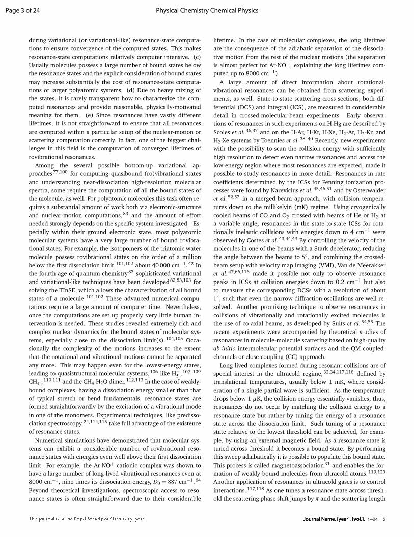
culated for NO–He at collision energies between 13 and 20 cm−1.Section 5 of the Supplement of Ref. 47 explains in detail howthe elements of the S-matrix are analyzed and how the resonantcontribution is separated from the background. As Fig. 5 illus-trates, this is done for individual elements of the S-matrix thatcorrespond to specific initial and final rotational states of NO. Itis interesting to observe in Fig. 5 that the energy dependence ofthe real and imaginary part of the S-matrix elements resemblesthe behavior of the complex energy eigenvalues of Fig. 11, videinfra, obtained with complex absorbing potentials. When the in-dividual S-matrix elements are thus disentangled, the effect ofa resonance on the ICSs and DCSs of all state-to-state inelasticprocesses can be calculated explicitly. The upper panel of Fig. 6shows that, indeed, the resonant peaks in the ICS disappear whenthe resonance contribution is removed, while the DCSs in thelower picture show that the resonances cause additional strong

20 21 22 23 24 25 26 27 28−2

−1

0

1

2

3

4

5

Energy [cm−1]

Phase shift / π

22+ channel openJ = 0

J = 1J = 2J = 3J = 4J = 5J = 6

20 21 22 23 24 25 26 27 28

0

20

40

60

80

100

Energy [cm−1]

Lifetime τ [5.31 ps] J = 0

J = 1J = 2J = 3J = 4J = 5J = 6

Fig. 7 Phase-shift sums Φ (top panel) and corresponding lifetimes (lowerpanel) as a function of the collision energy, calculated for NH3–He scat-tering. 174 The different curves correspond to different total angular mo-menta J, with the two curves for each J corresponding to even and oddoverall parity. This figure is reproduced from Ref. 174.

backward and near-forward scattering. Also the measured VMIimages are shown, next to simulated images obtained from thecalculated DCSs, with and without the resonant contributions. Itis clear that the agreement with the measurements is much lesssatisfactory for the latter, which confirms that the experiment in-deed detects resonance effects.

4.2.2 Phase shifts and resonance lifetimes

In a single-channel problem the S-matrix can simply be writtenas exp(2iφ), with the angle φ being the phase shift. In the multi-channel case S is a unitary matrix, its eigenvalues can be writtenas exp(2iφ (J)

n,l ), and the phase-shift sum Φ is the sum of φ(J)n,l over

all open channels.

It follows from theory4,5 that when a resonance occurs thephase shift (sum) rapidly increases by π as a function of thecollision energy E.172,173 This is illustrated in the top panel ofFig. 7 for the example of NH3–He scattering.174 Similar resultswere obtained for NH3–H2 scattering175 and OH–He scatter-ing.63 The derivative of the phase shift with respect to the energy,τ = hdΦ/dE, gives the lifetime of the collision complex.172,173

These lifetimes are shown in the lower panel of Fig. 7. This figureillustrates that at the energies where resonances occur one getsa long-lived collision complex. By comparing the peaks in thisfigure with the corresponding resonance peaks in the ICS (notshown for this example), one observes that the narrower the res-onance peak in the ICS, i.e., the smaller its width Γ , the longer itslifetime. This clearly confirms the relation τ = 1/Γ .



4.2.3 Adiabatic-bender model

The adiabatic-bender model, proposed by Alexander et al.176,177

and based on the Born–Oppenheimer angular-radial separation(BOARS),178 characterizes scattering resonances by adiabaticallyseparating the radial motion from the other dofs. The Hamilto-nian matrix without the radial kinetic energy term is diagonal-ized for all values of R, which yields a set of one-dimensional(1D) potentials depending on R, the adiabatic-bender curves.These curves asymptotically connect to the states of the separatedmonomers. In the next step one obtains 1D scattering states bysolving 1D scattering equations with each of these adiabatic po-tentials. If the adiabatic bender curves are sufficiently well sep-arated and do not change their character by avoided crossings,the full-dimensional scattering states can be associated with the1D states on each of the adiabatic bender curves and their char-acter follows for the monomer states to which the curves connectasymptotically. Thus, in the case of resonances, it can be deter-mined which monomer states participate in the resonance.

A recent example illustrating this method for OH–He and OH–Ne rotationally inelastic collisions is described in Ref. 63. The OHmonomer has a large rotational constant, its rotational states arefar apart, the adiabatic bender curves are well separated, and themethod works well. If one applies the method to NO–He, NO–H2

or O2–O2, for example, the much smaller rotational constants ofNO and O2 cause the set of adiabatic bender curves to becomerather dense, several avoided crossings occur between them, andthe connection to the monomer states is lost.

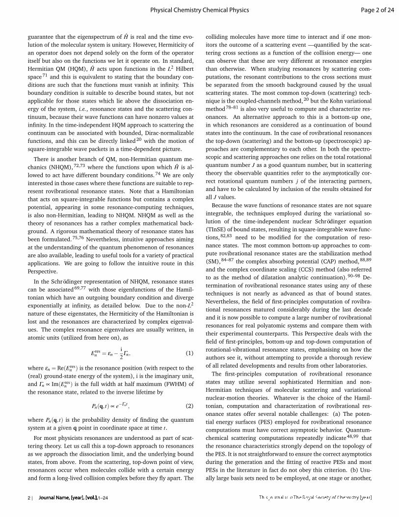
4.2.4 Analysis of scattering wave functions

With the renormalized Numerov propagator used in the Nijmegenscattering program to solve the CC equations, it is straightforwardto generate the scattering wave functions, not only asymptoticallybut over the full range of R. Thus, one can inspect the character ofthese wave functions in terms of the participating monomer statesand the end-over-end angular momentum l, the partial wave in-dex. If resonance peaks are observed in the ICS, one can deter-mine which total angular momenta J contribute most to thesepeaks, plot the wave functions for these values of J, and ana-lyze their character. This is illustrated in Fig. 8 for the exampleof NO–He scattering, already discussed in Sec. 4.2.1, where sev-eral resonances were calculated and observed experimentally47

for collision energies between 13 and 20 cm−1. The wave func-tions in Fig. 8 contain continuum states, but also have large am-plitudes in the region of the well of the NO–He potential, whichconfirms that they indeed correspond to quasi-bound states. Bothresonances shown correspond to the NO state j = 5/2, f . Sincethis channel is open at both resonance energies, they are shaperesonances. The resonance at 14.85 cm−1 corresponds to l = 5,the resonance at 17.75 cm−1 to l = 6. The excess collision energyis larger for the latter resonance and its continuum contributionis more pronounced, see Fig. 8.

4.2.5 S-matrix Kohn variational method

The S-matrix version of the Kohn variational method78–81,179,180

can also be applied to characterize scattering resonances, as wellas to investigate the sensitivity of the resonances to changes in

the PES. For a given J one writes a trial wave function as

ψn,l(R,ρ)=−φn,l(R)ϕn,l(ρ)+ ∑n′,l′

φ∗n′,l′(R)ϕn′,l′(ρ)Sn′,l′,n,l +∑

kχk(R,ρ)ck.

(57)The function φn,l(R) is an incoming wave at energy E − εn, thekinetic energy in channel n, the functions φ∗n′,l′(R) are the cor-

responding outgoing waves, and Sn′,l′,n,l are the elements of thetrial S-matrix. The incoming waves, φn,l(R), can be chosen freelyas long as they satisfy the Schrödinger equation at long rangeand are regularized at short range. The functions χk(R,ρ) forma bound-state basis. They are eigenfunctions of the Hamiltoniancomputed with the technique of discrete variable representation(DVR)181,182 on a finite R-grid and they provide flexibility in thetrial wavefunction in the region where φn,l(R)ϕn,l(ρ) does not al-ready solve the Schrödinger equation.

The trial wave function of Eq. (57) is optimized variationallyby considering first-order variations with respect to S and {ck},

δ 〈ψn,l |H−E|ψn,l〉= 2〈δψn,l |H−E|ψn,l〉+ iδ Sn,l,n,l . (58)

The bracket 〈 f |g〉 =∫

∞

0 dR∫

dρ f g is defined here without com-plex conjugation (see a similar trick in Sec. 6.3). An advantageof this approach is that the variational wave function is expressedas a linear combination of a scattering wave function and a set ofbound states at short range. Thus, one can analyze which boundstate gives rise to a scattering resonance by inspecting the opti-

0

4

8

12

5 10 15 20 25 30

R (bohr)

|Wav

efu

nct

ion

|2 (

a.u

.)

0

1

2

5 10 15 20 25 30

R (bohr)

|Wav

efu

nct

ion

|2 (

a.u

.)

Resonance II at 14.85 cm-1

Resonance III at 17.75 cm-1

a

b

(1/2 f ), 7

(1/2 e), 8

(3/2 e), 7

(3/2 e), 9

(3/2 f ), 6

(7/2 f ), 4

(5/2 f ), 5

(9/2 f ), 3

NO, l

(1/2 f ), 6

(1/2 e), 7

(3/2 e), 6

(3/2 e), 8

(3/2 f ), 5

(5/2 f ), 4

(3/2 f ), 7

(5/2 f ), 6

(7/2 f ), 5

NO, l

Fig. 8 Scattering wave functions of the NO–He system squared as afunction of the distance R. Panel a: At the resonance energy of 14.85cm−1 for J = 7.5 and P =+1. Panel b: At the resonance energy of 17.75cm−1 for J = 6.5 and P = −1. The rotational and Λ-doublet state of theNO radical, and the orbital angular momentum of the NO-He complex,are given for each curve. The states that dominate the resonances aremarked with a red box. This figure is reproduced from the Supplement ofRef. 47.



mized coefficients {ck}.This method was applied in a combined experimen-

tal/theoretical study of NO–He rotationally inelastic scatteringat very low collision energies, where resonances are found.116

The scattering cross sections calculated by the Kohn variationalmethod agree well with those from CC calculations and the as-signment of the resonances also agrees with the wave-functionanalysis described in Sec. 4.2.4. After establishing which quasi-bound states lead to particular resonances, one can estimate theresponse of the resonance energies to variations in the PES fromthe Hellman–Feynman theorem.183,184 In this way, it was ex-plored how sensitive the resonance energies are to overall scalingof the potential, to scaling of the correlation energy alone, to theanisotropy of the potential, and to a radial shift of the potential.

5 The stabilization method (SM)We begin the discussion of the various bottom-up approacheswith the stabilization method,84–87,185,186 which has a history ofat least 50 years85 and provides the simplest technique to iden-tify and characterize rovibrational resonances. The stabilizationmethod remains within the realm of variational techniques builtupon HQM and L2 functions. It is important to note right at thestart that SM allows the computation of not only resonance posi-tions, εn, but also resonance lifetimes, Γ−1

n .86,187

5.1 General background

The principal idea behind the SM technique is based on the ob-servation of stabilization of some of the eigenenergies in the (dis-cretized) continuum part of the eigenspectrum of the HermitianHamiltonian with respect to (slight) changes in selected compu-tational parameter(s), collectively named τ. During SM compu-tations the size of the basis or the coordinate range on the dis-sociation coordinate(s) is changed within a narrow interval. TheSM techniques differ by how the parameters are selected and howstabilization of certain eigenvalues of the Hermitian Hamiltonianis observed. It is important to emphasize that stabilization of res-onances is not an empirical observation but it is based on funda-mental properties of basic scattering theory. Stabilization can beunderstood via simple models of isolated resonances. A detailedexposure is given, for example, in Ref. 87.

In the stabilization method we approximate the eigenstatesabove the dissociation threshold by performing a number ofbound-state-type computations with slightly different values forthe computational parameter(s), τ. The wave function of a stableresonance state has large amplitudes localized within the interac-tion region of the fragments; thus, the energy is not sensitive tominor changes in the basis. Contrary to this, the continuum states(a) become “discretized” due to the finite range of the dissociationcoordinate, (b) are characterized by wave functions which havesignificant amplitude outside the deeper region of the potentialwell, and (c) have energies varying with the coordinate rangeand the type of the basis used. Thus, due to the large density ofcontinuum states around a resonance, minuscule changes in thebasis will yield minuscule change in the resonance energy, whilethe eigenenergies of continuum states will shift considerably.

Fig. 9 Overview of the stabilization-method (SM) histogram of Ar·NO+

in the 0–8000 cm−1 energy interval based on 25 separate vibrationalbound-state (L2) computations.

The traditional technique to observe resonances through theSM method employs En(τ) stabilization graphs, usually the prin-cipal outputs of SM computations. A resonance is observed whena plateau is seen in En(τ), a result of a slowly varying eigenvalue,identified as a resonance position. However, in the large basislimit, the density of states becomes infinite, and no plateau canbe observed in En(τ). In this case resonance energies are indi-cated by inflection points of the En(τ) curves. Another possibilityis to compute the expectation value of R2 (〈R2〉), where R is adissociation coordinate. Since 〈R2〉 is much smaller for resonancewave functions than for the discretized continuum states, 〈R2〉values provide good criteria for the identification of resonances.

In perhaps the simplest form of SM, identification of resonanceeigenvalues is achieved using the technique of histogram bin-ning.64 The TInSE computations are performed for a small num-ber of cases, say 25, with slightly different ranges along the dis-sociation coordinate. The eigenvalues are collected from all com-putations, and histograms are generated with a certain bin size.The horizontal axis corresponds to the binned energy scale, whilethe number of repeated simulations determines the count num-ber on the vertical axis of the histogram (see Fig. 9 for the case ofthe Ar·NO+ complex with an energy scale of 0–8000 cm−1). Asexpected, the smaller the bin size the better the performance ofthe method, a good choice in the case of tightly converged eigen-states is 0.001 cm−1. The stable resonance energies are indicatedby peaks on the histogram.

So far the SM technique has not been used in the Budapestgroup for the determination of resonance lifetimes. This is dueto the fact that this requires considerably more computational ef-fort than the determination of the positions. In the experienceof the Budapest group, the SM technique is quite successful inidentifying long-lived quasibound states. Finding resonances withshort lifetime may be difficult though as the energy of these statesis considerably more sensitive to computational parameters thanthose of the long-lived resonances. Furthermore, the CAP-basedand CCS techniques are much more appropriate to obtain a largenumber (if not all) resonances (both positions and lifetimes).



5.2 Application: SM analysis of the vibrational resonancesof Ar·NO+

During the study reported in Ref. 64 the SM method was usedto identify high-lying vibrational resonance states of the Ar·NO+

complex. In fact, the SM histogram of Fig. 9 represents the com-puted eigenvalues of the Ar·NO+ complex between 0 and 8000cm−1.64 Because the dissociation energy, D0, of the Ar·NO+ com-plex is 887 cm−1,64 the states with green color at the left of thefigure correspond to bound states. The bound states show a clearand well-defined termination upper limit at D0. The three furtherstacks between 2300–3200, 4600–5500, and 6900–7800 cm−1

show significant similarity with the stack corresponding to thebound states. They correspond to the first, second, and third ex-cited NO+ stretch states of Ar·NO+ and the width of each stack isapproximately D0 (with a very slight variation). Thus, Fig. 9 canbe explained via a very simple physical picture: the nearly idealadiabatic separation of the small-amplitude NO+ stretch motionfrom the other two, large-amplitude, intermonomer motions.

Pushing the computations to even higher NO+ stretch quantumnumbers is hindered by the extremely large number of eigenval-ues that would need to be computed variationally. In fact, Fig. 9 isbased on the first 12 000 vibrational eigenenergies of the Ar·NO+

system, computed iteratively.64

6 The complex absorbing potential (CAP)technique

Complex absorbing, or as sometimes called optical, poten-tials have been used both in the time-independent and time-dependent formulations of quantum mechanics. The CAP tech-nique56,88,89,188–193 is probably the most commonly used ap-proach to compute rovibrational resonance states. In the CAPtechnique the rovibrational Hermitian Hamiltonian is “perturbed”with a complex potential, introduced to absorb the outgoing partof the resonance eigenfunctions, making them square integrable.This approximation to resonance wave functions employs an ex-pansion using an L2 basis, e.g., the bound states and the eigen-states with energies above dissociation originating from a bound-state computation. Even though CAP-perturbed Hamiltonians acton square-integrable functions, it is not a Hermitian formalism be-cause of the complex potential. Ref. 88 explores the CAP methodand its properties with mathematical rigor, while a more generalreview of the CAP technique can be found in Ref. 89.

6.1 General backgroundThe modified CAP Hamiltonian can be written as

H′(η) = H− iηW (R), (59)

where H is the unperturbed and H ′ is a complex Hamiltonian, η

is the CAP-strength parameter, and W (R) is usually a real-valuedfunction of the R dissociation coordinate assuming nonzero valuesat the asymptotic region of the PES (more than one dissociationcoordinate, of course, is also feasible). Complex valued W (R) CAPfunctions have also been studied.194

A useful approach emerges when the CAP-perturbed non-Hermitian Hamiltonian is represented in the basis of the eigenvec-

tors computed with a bound-state code up to and above the firstdissociation threshold. Some of the eigenvalues of the complexmatrix representation of H′(η) are approximations to the true res-onance energies. The resonance eigenenergies are characterizedby two sources of error. The first error is caused by the presenceof the CAP function added to the Hamiltonian. This error is smallfor small η values and large for large η values. The second erroris the basis set error, arising because we try to represent a non-square-integrable function with L2 basis functions. This type oferror becomes small for sufficiently large η values, and remainslarge if the η value is small and the wave function is not dampedsufficiently.

To find an optimal η value, where the two types of error ei-ther cancel each other out or at least their sum becomes minimal,eigenvalue trajectories in the complex plane need to be generatedby varying the CAP-strength parameter. Resonance cusps withinthe trajectories are then detected and they are associated withan optimal η , yielding resonance positions and lifetimes. Here“cusp” means that there is a sharp bend (local maximum of thecurvature) on the trajectory and the density of points has a maxi-mum.

The efficiency of different types of CAP functions has been in-vestigated in a number of studies and various recommendationshave been made; see, for example, Refs. 192–198. In our ownexperience, if the applied L2 basis set is large enough, then theresonance eigenvalues are not particularly sensitive to the spe-cific form of the CAP function used (as long as the CAP functionhas significant magnitude in the coordinate ranges, appropriatefor absorbing the outgoing part of the wave function).

6.2 GENIUSH-CAP

One implementation of the CAP method for the computation ofrotational-vibrational resonance states of arbitrary systems is partof the GENIUSH-CAP code.65 One needs to perform one expen-sive bound-state-type computation with the bound-state code GE-NIUSH,146,147 which solves TInSE quasi-variationally, in order tocompute energies and wave functions above the first dissociationthreshold. The GENIUSH eigenvectors are then used as a basis tobuild the matrix of H′(η), whose complex eigenvalues are finallycomputed. Repeating this for a few hundred η values leads tocomplex eigenvalue trajectories. In the traditional CAP methodvisual analysis is used to identify resonance cusps in the trajecto-ries.

The CAP approach has several advantages over the stabiliza-tion method. First, in the case of the SM technique one needsto perform a few tens of variational bound-state computations,which can take a considerable amount of computer time, whilethe CAP technique may require only one expensive bound-statecomputation. Second, the follow-up computation of CAP trajec-tories is inexpensive, because the matrix of the modified Hamilto-nian H′(η) is much smaller than that of the original Hamiltonian,H. Third, the CAP method is significantly better suited to identifyboth short- and long-lived resonances.

When compared to the complex coordinate scaling (CCS) tech-nique, see Sec. 7, the CAP technique has another major advan-



tage: the CAP changes only the potential-energy part of theHamiltonian. Thus, CAP-based techniques do not require theknowledge of the Hamiltonian in an analytic form and the CAPtechnique can be incorporated straightforwardly into numericaltechniques based upon the discrete variable representation181,182

of the Hamiltonian. This is exactly why we decided to extendour fourth-age quantum-chemical83 code GENIUSH,146,147 builtupon the DVR representation of the Hamiltonian, with the CAPcapability.

The only considerable drawback of the CAP method is the needfor visual searches for cusps. This takes a lot of human effort, andintroduces some subjectivity to the collection of resonance states.There have been some reports about automatic cusp recognition,e.g., the method of Silva et al.62 There the cusps are identifiedbased on the curvature of the CAP trajectories and the density ofthe points. In our experience it is easy to either miss rovibrationalresonances or to assign false positives this way. Thus, we consid-ered another approach for automating CAP computations, namedthe extended Tremblay–Carrington (ETC) method,61,68 discussedin the next subsection.

6.3 The ETC method

The principal advantage of the ETC method68 is that it makes thecomputation of rovibrational resonance states automatic. Usingthe ETC method the resonance energies are obtained as eigenval-ues of an unmodified Hamiltonian matrix built in a suitable basis,which is composed of selected eigenvectors of a CAP computa-tion. This way one completely circumvents the computation ofCAP trajectories.

The algorithm of the ETC method is as follows. First, solvea CAP-type eigenvalue equation with a suitable CAP-strength pa-

Fig. 10 Stabilization-method (SM) histogram of Ar·NO+, with a bin sizeof 0.01 cm−1, within the energy range 20 cm−1 above the first disso-ciation limit, D0(ArNO+)=887 cm−1. Eigenvalues are obtained from 25GENIUSH computations.

rameter, ηguide,

H ′(ηguide) |φk〉= (H− iηguideW (R)) |φk〉= Ek |φk〉 . (60)

This step can be performed, among others, with the GENIUSH-CAP code.65 Second, select carefully a basis set {|φk〉} from theeigenvectors obtained in step (1). This is a very important step asone must choose only those eigenvectors which became square-integrable due to the CAP, i.e., they are small where the CAPfunction is large. As shown in Ref. 68, selection of the basis{|φk〉} can be done more or less automatically, based on the com-plex eigenvalues Ek. The basis functions are normalized suchthat 〈φ∗k |φl〉 = δkl , contrary to the conventional normalization〈φk|φl〉 = δkl . Third, one builds the matrix of the original Hamil-tonian in this basis,

Hkl = 〈φ∗k |H|φl〉 , (61)

and solves the eigenvalue equation. The Hamiltonian matrix builtthis way is clearly not Hermitian and thus it has complex eigen-values. Furthermore, there are more basis functions than reso-nances. In order to identify which complex eigenvalues belongto resonance states, we repeat the three steps described, with afew (let’s say 11) slightly different ηguide values. The resonanceeigenvalues are less sensitive to the choice of ηguide than the onesthat do not correspond to resonance states. If we plot the com-puted eigenenergies resulting from all ηguide values on the com-plex plane, they form well-defined clusters. The points withina cluster belong to the same state but they are obtained withdifferent ηguide values. Eigenvalues corresponding to resonancestates form compact clusters, while the non-resonance eigenval-ues form clusters that are considerably more extended. In orderto make this approach automatic, clusters must be characterizedby suitable algorithms facilitating their observation. For a suit-able choice of a scoring algorithm Ref. 68 should be consulted, inwhich appraisal scores are assigned to each cluster to guide theselection of resonance states.

Because the computations following the usually expensivebound-state computation are inexpensive, due to the small sizeof the Hamiltonian matrix built with the carefully selected {|φk〉}basis, the additional computations with different ηguide values donot increase the overall cost of the determination of rovibrationalresonances via the ETC method at all.

6.4 Applications

6.4.1 Vibrational resonances of Ar·NO+

In Ref. 64, not only the SM but also a CAP-based method (and ascattering method, see above) was used to identify and character-ize the resonance states of the Ar·NO+ complex. The long-livedresonance states found by the SM method (see Fig. 10) havebeen confirmed by the GENIUSH-CAP method as states with longlifetimes when compared to the other resonance states in theirvicinity.

Fig. 11 shows a few selected GENIUSH-CAP eigenvalue trajec-tories with various forms of cusps. The three different colors indi-cate the different basis set sizes along the Ar–NO+ distance usedin the bound-state-type GENIUSH computation, thereby reflect-



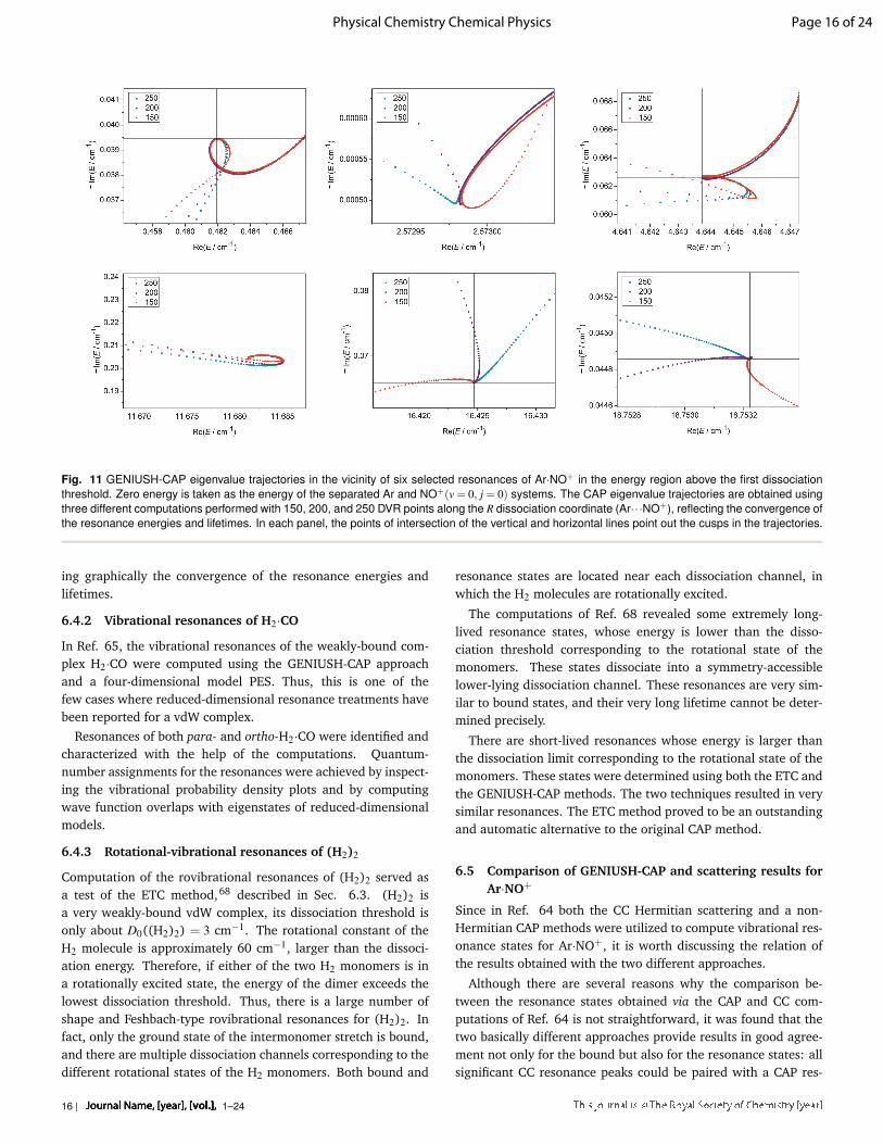
Fig. 11 GENIUSH-CAP eigenvalue trajectories in the vicinity of six selected resonances of Ar·NO+ in the energy region above the first dissociationthreshold. Zero energy is taken as the energy of the separated Ar and NO+(v = 0, j = 0) systems. The CAP eigenvalue trajectories are obtained usingthree different computations performed with 150, 200, and 250 DVR points along the R dissociation coordinate (Ar· · ·NO+), reflecting the convergence ofthe resonance energies and lifetimes. In each panel, the points of intersection of the vertical and horizontal lines point out the cusps in the trajectories.

ing graphically the convergence of the resonance energies andlifetimes.

6.4.2 Vibrational resonances of H2·CO

In Ref. 65, the vibrational resonances of the weakly-bound com-plex H2·CO were computed using the GENIUSH-CAP approachand a four-dimensional model PES. Thus, this is one of thefew cases where reduced-dimensional resonance treatments havebeen reported for a vdW complex.

Resonances of both para- and ortho-H2·CO were identified andcharacterized with the help of the computations. Quantum-number assignments for the resonances were achieved by inspect-ing the vibrational probability density plots and by computingwave function overlaps with eigenstates of reduced-dimensionalmodels.

6.4.3 Rotational-vibrational resonances of (H2)2

Computation of the rovibrational resonances of (H2)2 served asa test of the ETC method,68 described in Sec. 6.3. (H2)2 isa very weakly-bound vdW complex, its dissociation threshold isonly about D0((H2)2) = 3 cm−1. The rotational constant of theH2 molecule is approximately 60 cm−1, larger than the dissoci-ation energy. Therefore, if either of the two H2 monomers is ina rotationally excited state, the energy of the dimer exceeds thelowest dissociation threshold. Thus, there is a large number ofshape and Feshbach-type rovibrational resonances for (H2)2. Infact, only the ground state of the intermonomer stretch is bound,and there are multiple dissociation channels corresponding to thedifferent rotational states of the H2 monomers. Both bound and

resonance states are located near each dissociation channel, inwhich the H2 molecules are rotationally excited.

The computations of Ref. 68 revealed some extremely long-lived resonance states, whose energy is lower than the disso-ciation threshold corresponding to the rotational state of themonomers. These states dissociate into a symmetry-accessiblelower-lying dissociation channel. These resonances are very sim-ilar to bound states, and their very long lifetime cannot be deter-mined precisely.

There are short-lived resonances whose energy is larger thanthe dissociation limit corresponding to the rotational state of themonomers. These states were determined using both the ETC andthe GENIUSH-CAP methods. The two techniques resulted in verysimilar resonances. The ETC method proved to be an outstandingand automatic alternative to the original CAP method.

6.5 Comparison of GENIUSH-CAP and scattering results forAr·NO+

Since in Ref. 64 both the CC Hermitian scattering and a non-Hermitian CAP methods were utilized to compute vibrational res-onance states for Ar·NO+, it is worth discussing the relation ofthe results obtained with the two different approaches.

Although there are several reasons why the comparison be-tween the resonance states obtained via the CAP and CC com-putations of Ref. 64 is not straightforward, it was found that thetwo basically different approaches provide results in good agree-ment not only for the bound but also for the resonance states: allsignificant CC resonance peaks could be paired with a CAP res-



Fig. 12 Illustration of the eigenvalues of a complex-scaled Hamiltonianin the vicinity of one dissociation channel. The blue and purple arrowspoint out the bound and resonance eigenvalues, respectively, while thered arrow points out the rotated scattering continuum.

onance within a few 0.1 cm−1 (the expected agreement of theresults obtained with the two techniques). The lifetimes obtainedas the eigenvalues of the close-coupling Smith lifetime matrix andGENIUSH-CAP lifetimes also showed reasonable agreement forthe longer-lived resonances.

7 The complex coordinate scaling (CCS)method

7.1 General backgroundIn the non-Hermitian CCS scheme rovibrational resonance statesare computed as the exponentially diverging solutions of theTInSE, see Eq. (50). Within the CCS scheme one introduces aninvertible operator S, so that the functions Φn = SΨres

n becomesquare integrable. The similarity-transformed Schrödinger equa-tion reads as

SHS−1Φn = Eres

n Φn, Φ ∈ L2. (62)

Eq. (62) is an eigenvalue equation for the transformed Hamil-tonian SHS−1, whereby the eigenfunctions are square integrableand the eigenvalues are the desired resonance eigenenergies. Eq.(62) can be solved with the well-developed L2 techniques ofquantum chemistry.

In the conventional CCS method, a choice for the operator S is

Sθ f (R) = f (Reiθ ), (63)

where θ is a free parameter and R is the dissociation coordi-nate. Therefore, the operator Sθ rotates the argument of a func-tion of the dissociation coordinate by θ in the complex plane.If there is more than one dissociation coordinate, each shouldundergo a complex coordinate scaling transformation. Due tothe transformation by Sθ ,77,90–92,96,97 (a) resonance states forwhich 2θ > arctan(Γ /(2(ε −D0))) = Arg(Eres−D0) will becomesquare integrable, (b) bound states remain square integrable forθ < π/4 (which is true in all practical applications), and (c) thescaled Hamiltonian has scattering eigenfunctions which are as-sociated with a continuum that is rotated into the lower half ofthe complex energy plane by the angle 2θ .91,92,96,97 Thus, in thespectrum of the scaled Hamiltonian of Eq. (62), (a) real discrete

eigenvalues (unaffected by the CCS) correspond to bound states,(b) the scattering continuum is rotated into the lower half of thecomplex plane by 2θ for each dissociation channel, and (c) dis-crete complex eigenvalues in the area between the real axis andthe rotated scattering continua correspond to resonance states,see Fig. 12.

Obtaining the form of the scaled Hamiltonian is rather straight-forward in the case of conventional complex scaling. For differen-tial operators corresponding to the dissociation coordinate R, oneneeds to make the change ∂

∂R →∂

∂R e−iθ . For operators depend-ing only on the coordinate the change R→ Reiθ is required.96,97

In its simplest form, CCS requires a PES that can be evaluated atcomplex coordinate values, which can be achieved for PESs hav-ing a fitted analytical form, once one rewrites the PES subroutineinto complex arithmetic. In addition, various techniques, also ap-plicable for non-analytical PESs, are available; for examples, seeRefs. 98, 199, and 200.

Somewhat more involved but often more convenient and nu-merically more efficient extensions of the CCS method have beendeveloped. These include the method of exterior complex scal-ing,201,202 whereby the transformation is defined, for R≥ Rs, as

Sθ f (R) = f (Rs + eiθ (R−Rs)). (64)

The exterior complex scaling transformation has been imple-mented for grid-based techniques,203,204 and a smooth exteriorcomplex scaling method73 has also been advocated. Note thatthe CAP method can be derived from smooth exterior complexscaling by applying certain approximations.73,205

Naturally, resonance eigenenergies with a physical meaningshould be independent of the scaling parameter θ in Eq. (63).However, in practice, when finite basis sets are used, the formof the Φn eigenfunctions and thus the “goodness” of the basisdepends on the scaling parameter. Similar to the CAP method,resonance eigenenergies can be identified in the CCS formalismby locating stationary points in eigenvalue trajectories obtainedby varying the scaling parameter θ .

7.2 Applications

7.2.1 Rotational-vibrational resonances of H216O

H216O is a strongly-bound molecule for which rovibrational res-

onance states have been identified experimentally.12 Therefore,performing rovibrational resonance computations for this speciesis extremely important to test the utility of the different tech-niques. In Ref. 13 the spectrum of H2

16O was simulated abovethe first dissociation threshold using advanced electronic struc-ture and nuclear motion computations, and the simulated spec-trum was compared to the experimental one from Ref. 12. Sev-eral Feshbach and shape resonances were determined with theCAP method, and a broad spectral feature resulting from the di-rect photodissociation to the continuum was also revealed in thisstudy.

In Ref. 14 the low-lying rovibrational resonances of H216O were

computed using the CCS method. During these calculations thematrix representation of the scaled Hamiltonian was obtained in



Fig. 13 Eigenvalue trajectories of H2He+ on the complex energy plane, obtained by varying the scaling parameter of the complex coordinate scaling(CCS) method between 0.02 and 0.80 in 40 steps. See Ref. 67 for computational details.

two steps. First, all the bound states of the unscaled Hamilto-nian were computed, using the code D2FOPI,104 along with manyeigenpairs having energies above the dissociation threshold. Inthe second step, using a subset of the computed eigenvectors asan orthonormal basis set, the matrix of the scaled Hamiltonianwas constructed,

Hθkl = 〈Ψk|Sθ HS−1

θ|Ψl〉 , (65)

resulting in a matrix with modest size, on the order of around athousand-by-thousand, which could be directly diagonalized forthe few dozen θ values required to form the complex eigenvaluetrajectories. Inspection of the vibrational probability density plotsfrom the stationary resonance calculations revealed several typesof (dynamical) dissociation behavior, varying among the states.The calculations aided the proper assignment of some observedrovibrational transitions beyond the first dissociation threshold ofH2

16O.13

7.2.2 Rotational-vibrational resonances of H2He+

In Ref. 67, a large number of rovibrational resonances has beencomputed and characterized for the H2He+ molecular ion, usingthe CCS, the CAP, and the SM techniques. These accurate com-putations of the bound and resonance states facilitate the firstexperimental observation of rovibrational transitions of this fun-damental molecule, made up of the two most abundant elementsof the universe. The CCS algorithm employed was basically thesame as that detailed for H2

16O in the previous subsection. Fig.13 shows some CCS eigenvalue trajectories computed in Ref. 67,reflecting a number of dissociation channels, corresponding tothe different rotational states of the H+

2 moiety in the dissociatedsystem.

Beyond the spectroscopic data, valuable for future high-resolution experiments, the quantum-chemical computations onH2He+ also revealed dissociation pathways, dissociation branch-ing ratios, and the stabilization mechanism of the long-lived res-onances. Because the H–H stretching fundamental lies above thefirst dissociation threshold of H2He+, D0(H2He+) = 1775.4 cm−1,

resonances are expected to play a crucial role in the collision andassociation reactions involving H2He+, including radiative asso-ciation and radiative charge-transfer reactions. Fig. 14 showsthe probability density plot of a selected vibrational resonance ofH2He+, computed in Ref. 67. The resonance shown in Fig. 14is a Feshbach resonance, in which the H+

2 moiety is rotationallyhighly excited in the interaction region.

Fig. 14 The nodal structure of a J = 0 vibrational resonance state ofH2He+ located at around 2109.4 cm−1 above its zero-point vibrationalenergy, where R2 and θ denote the H+

2 −He distance and the Jacobi angledefined by the H+

2 −He and H−H bonds, respectively. See Ref. 67 forcomputational details.



Fig. 15 Calculated potential energy curves along a C−H stretching coor-dinate of the planar ethylene dication, C2H+

4 . The gray dotted line showsthe electronic ground state, while the blue solid line and the green dashedline correspond to the first and second electronically excited states, re-spectively. Horizontal lines represent vibrational states. See Ref. 206 forcomputational details.

7.2.3 Understanding the ultraslow decay in Coulomb explo-sion of hydrocarbons

In the experiments described in Ref. 206, the C2H2+2 and C2H2+

4dications were generated by double ionization with few-cycle in-tense laser pulses. In the deprotonation pathway of the Coulombexplosion for both C2H2+

2 and C2H2+4 , an ultraslow, microsecond

timescale exponential decay channel was observed.Reduced-dimensional resonance-state computations,206 utiliz-

ing the CCS method, revealed that in both cases the slow decaychannel is due to quasibound states along the C–H vibrationalmode, where tunneling through a barrier is responsible for theexponential decay, see Fig. 15.

8 Summary and outlookThe extremely rich internal dynamics of molecular systems justbelow and above the first dissociation threshold can be studiedwith a variety of quantum-chemical bound, resonance, and scat-tering techniques employing accurate potential energy surfaces,corresponding usually to the ground electronic state and exhibit-ing correct asymptotic behavior. This Perspective focuses on thefirst-principles computation and characterization of rovibrationalresonances, proving that, depending on the chemistry, getting to-gether or breaking up are complex processes even for molecularsystems.

Most rovibrational resonance states can be categorized basedon their physical origin, they can be shape or Feshbach-type res-onances. One can approach resonance states either from thedirection of bound states (a bottom-up approach) or from scat-tering states (a top-down approach). Next, we concentrate firston the bottom-up and then on the top-down first-principles ap-proaches. Then we give some information about experiments re-lated to rovibrational resonance states.

The complex algorithms and codes developed for bound-state

computations during the fourth age of quantum chemistry aresuitable to determine and describe the numerous L2 bound rovi-brational states. As to resonances, the stabilization method (SM)allows the utilization of bound-state computations to determinelong-lived resonances (both their position and lifetime). The SMmethod is based on the fact that the eigenenergies of a HermitianHamiltonian corresponding to resonances are rather insensitiveto slight changes in certain parameters of the bound-state-typecomputation. Thus, if one can perform a considerable numberof bound-state computations yielding a large number of unboundstates, a histogram binning approach can be utilized to identifylong-lived resonances among the unbound states in a straightfor-ward manner.

Apart from the simple “trick” of repeating them many times,bound-state variational approaches are unsuitable for the com-putation of resonances without appropriate modifications. Thereare two basic routes one can take, both are based on the regular-ization of the diverging resonance wave functions. In the case ofthe complex absorbing potential (CAP) method, the outgoing partof the wave function is damped by a complex potential added tothe molecular PES along the dissociative mode(s). The CAP en-sures that resonance wave functions can be expanded in an L2

basis. A variant of the CAP methods, the extended Tremblay–Carrington (ETC) scheme allows an almost automatic (black-box-type) determination of rovibrational resonances. Since the ETCmethod can be coupled to the best general-purpose solvers ofthe time-independent nuclear Schrödinger equation, the result-ing algorithm and code is available to compute rovibrational res-onances of larger systems, perhaps in reduced dimension, in asemi-automatic way.

The alternative complex coordinate scaling (CCS) technique in-volves a complex coordinate transformation along the dissocia-tion degree of freedom. Most variants of this technique requirethe availability of the Hamiltonian, including the PES, in an ana-lytic form, which is usually not a significant restriction.

Variants of the SM, the CAP, and the CCS techniques have beensuccessfully applied by members of the Budapest group for sev-eral small systems, such as triatomic molecules (the strongly-bound H2

16O and H2He+), atom-diatom complexes (Ar·NO+),diatom-diatom complexes (H2·CO and (H2)2), and small cationicsystems (C2H2+

2 and C2H2+4 ).

The scattering problem can also be solved using differentfirst-principles techniques. The coupled-channels (or sometimescalled close-coupling) technique employs a Hermitian Hamilto-nian and a coupled-channel basis corresponding to the differentquantum states of the colliding molecules and products. Thecoupled-channels equations are solved by numerical integration.In the case of the Kohn variational method the trial wave func-tion, which contains both scattering basis functions and boundstate basis functions, is optimized variationally. Sometimes theadiabatic-bender model is applicable to simplify the scatteringproblem. This is achieved by separating the radial motion fromthe rotation and vibration of the colliding molecules. Solving thescattering problem results in the scattering matrix and state-to-state integral and differential cross sections. By analyzing theenergy-dependent elements of the scattering matrix, one can sep-



arate the contribution of the resonances from the contribution ofthe background. Resonances can be characterized either by thecomplex poles of the scattering matrix, peaks of the integral scat-tering cross section, or the sharp increase of the phase shift by π

as a function of energy. These scattering computations have beenemployed to investigate the resonances in systems such as NH3–He, NH3–H2, NO–He, NO–H2, OH–He, OH–Ne, and H2–He∗.

Several techniques which can yield experimental informationabout rotational-vibrational resonances are available. There isa plethora of crossed molecular beam experiments, starting inthe 1960s,207 which are able to yield detailed results about res-onances. Depending upon its resolution, photoelectron velocity-map imaging spectroscopy may provide spectra with a wealth ofinformation about Feshbach resonances. Scattering experimentsare becoming increasingly sophisticated, as state-selective prepa-ration of reactants, state-resolved detection of products, as well asvelocity and angle resolution of both reactants and products aremore and more feasible. As the computational tools for describingrovibrational resonances of polyatomic molecules become evermore efficient and sophisticated, they are expected to play an in-creasing role in supporting the high-resolution spectroscopy ofmolecules near and above their dissociation threshold, the exper-imental efforts in molecular dynamics, including those inducedby strong fields, as well as ever more complex scattering experi-ments.

Finally, we mention that Feshbach resonances may play arole in at present exotic applications, such as the production of(molecular) Bose–Einstein condensates.208 As explained in theIntroduction, it is important for this application that resonancesin ultracold collisions can be manipulated with external electricand/or magnetic fields. The manipulation of resonances by ex-ternal electric and magnetic fields is also of more general inter-est, since it may open up new possibilities to steer the outcomeof reactive and non-reactive collisions, photochemical reactions,unimolecular decay, etc., as shown for model systems and real-istic systems alike; see, for example, Refs. 209–213. Crossedmolecular beam studies of low-energy molecule-molecule colli-sions in external fields to explore these possibilities are beingprepared.214 Some related preliminary calculations have alreadybeen performed.215–218

Conflicts of interest

There are no conflicts of interest to declare.

Acknowledgements

The work performed by AGC and TS received support from NKFIH(grants no. K119658 and PD124623, respectively). The work ofIS was supported partially by the ÚNKP-19-3 New National Excel-lence Program of the Ministry for Innovation and Technology ofHungary. The research of the Budapest group was also supportedby the European Union and the State of Hungary and co-financedby the European Regional Development Fund (Grant no. VEKOP-2.3.2-16-2017-00014). TK is supported by NWO Rubicon GrantNo. 019.172EN.007 and the NSF through ITAMP.

References1 G. Gamow, Z. Phys., 1928, 51, 204–212.2 O. K. Rice, J. Chem. Phys., 1933, 1, 375–389.3 U. Fano, Nuovo Chim., 1935, 12, 154–161.4 G. Breit and E. P. Wigner, Phys. Rev., 1936, 49, 519–531.5 A. F. J. Siegert, Phys. Rev., 1939, 56, 750–752.6 H. Feshbach, Ann. Phys., 1958, 5, 357–390.7 C. Mahaux, in Lecture Notes in Physics, ed. S. Albeverrio, L. S.

Ferreia and L. Streit, Springer-Verlag, Berlin, 1984, vol. 211.8 H. Feshbach, Theoretical Nuclear Physics: Nuclear Reactions,

Wiley, New York, 1992.9 L. Fonda and R. G. Newton, Ann. Phys., 1960, 10, 490–515.

10 M. Qiu, Z. Ren, L. Che, D. Dai, S. A. Harich, X. Wang, X. Yang,C. Xu, D. Xie, M. Gustafsson, R. T. Skodje, Z. Sun and D. H.Zhang, Science, 2006, 311, 1440–1443.

11 D. H. Zhang and H. Guo, Annu. Rev. Phys. Chem., 2016, 67,135–158.

12 M. Grechko, P. Maksyutenko, T. R. Rizzo and O. V. Boyarkin,J. Chem. Phys., 2010, 133, 081103.

13 N. F. Zobov, S. V. Shirin, L. Lodi, B. C. Silva, J. Tennyson,A. G. Császár and O. L. Polyansky, Chem. Phys. Lett., 2011,507, 48–51.

14 T. Szidarovszky and A. G. Császár, Mol. Phys., 2013, 111,2131–2146.

15 B. K. Kendrick, L. Jayasinghe, S. Moser, M. Auzinsh andN. Shafer-Ray, Phys. Rev. Lett., 2000, 84, 4325–4328.

16 G. C. Schatz, Science, 2000, 288, 1599–1600.17 M. L. Weichman, J. A. DeVine, M. C. Babin, J. Li, L. Guo,

J. Ma, H. Guo and D. M. Neumark, Nat. Chem., 2017, 9,950–955.

18 S. A. Reid and H. Reisler, Annu. Rev. Phys. Chem., 1996, 47,495–525.

19 G. J. Schulz, Phys. Rev. Lett., 1963, 10, 104–105.20 J. R. Taylor, Scattering Theory, Wiley, New York, 1972.21 J.-M. Hartmann, C. Boulet and D. Robert, Collisional Effects

on Molecular Spectra, Elsevier, 2008.22 W. G. Brown and G. E. Gibson, Phys. Rev., 1932, 40, 529–

543.23 J. M. Hutson, C. J. Ashton and R. J. Le Roy, J. Phys. Chem.,

1983, 87, 2713–2720.24 M. Okamura, L. I. Yeh and Y. T. Lee, J. Chem. Phys., 1985,

83, 3705–3706.25 C. J. Ashton, M. S. Child and J. M. Hutson, J. Chem. Phys.,

1983, 78, 4025–4039.26 U. Fano, Phys. Rev., 1961, 124, 1866–1878.27 W. Domcke, Phys. Rep., 1991, 208, 97–122.28 R. Schinke, Photodissociation Dynamics, Cambridge Univer-

sity Press, Cambridge, 1993.29 H. M. Yin, S. H. Kable, X. Zhang and J. M. Bowman, Science,

2006, 311, 1443–1446.30 K. M. Jones, E. Tiesinga, P. D. Lett and P. S. Julienne, Rev.

Mod. Phys., 2006, 78, 483–535.31 T. Köhler, K. Góral and P. S. Julienne, Rev. Mod. Phys., 2006,



78, 1311–1361.32 D. W. Chandler, J. Chem. Phys., 2010, 132, 110901.33 Y. Wang and P. S. Julienne, Nat. Phys., 2014, 10, 768–773.34 N. Balakrishnan, J. Chem. Phys., 2016, 145, 150901.35 R. N. Zare, Science, 2006, 311, 1383–1385.36 A. Schutte, G. Scoles, F. Tommasini and D. Bassi, Phys.Rev.

Lett., 1972, 29, 979–982.37 A. Schutte, D. Bassi, F. Tommasini and G. Scoles, J. Chem.

Phys., 1975, 62, 600–605.38 J. P. Toennies, W. Welz and G. Wolf, J. Chem. Phys., 1974,

61, 2461–2462.39 J. P. Toennies, W. Welz and G. Wolf, J. Chem. Phys., 1976,

64, 5305–5307.40 J. P. Toennies, W. Welz and G. Wolf, J. Chem. Phys., 1979,

71, 614–642.41 R. E. Wyatt and M. J. Redmon, Chem. Phys. Lett., 1983, 96,

284–288.42 P. Maksyutenko, T. R. Rizzo and O. V. Boyarkin, J. Chem.

Phys., 2006, 125, 181101.43 S. Chefdeville, T. Stoecklin, A. Bergeat, K. M. Hickson,

C. Naulin and M. Costes, Phys. Rev. Lett., 2012, 109, 023201.44 S. Chefdeville, Y. Kalugina, S. Y. T. van de Meerakker,

C. Naulin, F. Lique and M. Costes, Science, 2013, 341, 1094–1096.

45 A. B. Henson, S. Gersten, Y. Shagam, J. Narevicius andE. Narevicius, Science, 2012, 338, 234–238.

46 E. Lavert-Ofir, Y. Shagam, A. B. Henson, S. Gersten, J. Kłos,P. S. Zuchowski, J. Narevicius and E. Narevicius, Nat. Chem.,2014, 6, 332–335.

47 S. N. Vogels, J. Onvlee, S. Chefdeville, A. van der Avoird,G. C. Groenenboom and S. Y. T. van de Meerakker, Science,2015, 350, 787–790.

48 T. Yang, J. Chen, L. Huang, T. Wang, C. Xiao, Z. Sun, D. Dai,X. Yang and D. H. Zhang, Science, 2015, 347, 60–63.

49 A. Bergeat, J. Onvlee, C. Naulin, A. van der Avoird andM. Costes, Nat. Chem., 2015, 7, 349–353.

50 M. Beyer and F. Merkt, Phys. Rev. Lett., 2016, 116, 093001.51 A. Klein, Y. Shagam, W. Skomorowski, P. S. Zuchowski,

M. Pawlak, L. M. C. Janssen, N. Moiseyev, S. Y. T. van deMeerakker, A. van der Avoird, C. P. Koch and E. Narevicius,Nat. Phys., 2017, 13, 35–38.

52 J. Zou, S. D. S. Gordon, S. Tanteri and A. Osterwalder, J.Chem. Phys., 2018, 148, 164310.

53 S. D. S. Gordon, J. J. Omiste and A. Osterwalder, Nat. Chem.,2018, 10, 1190–1195.

54 C. Amarasinghe, H. Li, C. A. Perera, M. Besemer, A. van derAvoird, G. C. Groenenboom, C. Xie, H. Guo and A. G. Suits,J. Phys. Chem. Lett., 2019, 10, 2422–2427.

55 C. Amarasinghe, H. Li, C. A. Perera, M. Besemer, A. van derAvoird, G. C. Groenenboom, J. Zuo, C. Xie, H. Guo, J. Kłosand A. G. Suits, Nat. Chem., 2020, accepted,.

56 D. Wang and J. M. Bowman, J. Chem. Phys., 1994, 100,1021–1027.

57 H.-J. Werner, C. Bauer, P. Rosmus, H.-M. Keller, M. Stumpfand R. Schinke, J. Chem. Phys., 1995, 102, 3593–3611.

58 V. Ryaboy and N. Moiseyev, J. Chem. Phys., 1995, 103,4061–4068.

59 V. A. Mandelshtam and H. S. Taylor, J. Chem. Phys., 1997,106, 5085–5090.

60 B. Poirier and T. Carrington Jr., J. Chem. Phys., 2002, 116,1215–1227.

61 J. Tremblay and T. Carrington, J. Chem. Phys., 2005, 122,244107.

62 B. C. Silva, P. Barletta, J. J. Munro and J. Tennyson, J. Chem.Phys., 2008, 128, 244312.

63 K. B. Gubbels, Q. Ma, M. Alexander, P. Dagdigian, D. Tanis,G. C. Groenenboom, A. van der Avoird and S. Y. T. van deMeerakker, J. Chem. Phys., 2012, 136, 144308.

64 D. Papp, J. Sarka, T. Szidarovszky, A. G. Császár, E. Mátyus,M. Hochlaf and T. Stoecklin, Phys. Chem. Chem. Phys., 2017,19, 8152–8160.

65 D. Papp, T. Szidarovszky and A. G. Császár, J. Chem. Phys.,2017, 147, 094106.

66 S. N. Vogels, T. Karman, J. Kłos, M. Besemer, J. Onvlee,A. van der Avoird, G. C. Groenenboom and S. Y. T. van deMeerakker, Nat. Chem., 2018, 10, 435–440.

67 D. Papp, A. G. Császár, K. Yamanouchi and T. Szidarovszky,J. Chem. Theory Comput., 2018, 14, 1523–1533.

68 I. Simkó, T. Szidarovszky and A. G. Császár, J. Chem. TheoryComput., 2019, 15, 4156–4169.

69 L. D. Landau and E. M. Lifshitz, Quantum Mechanics, 3rd ed.,Pergamon, Oxford, 1977.

70 R. McWeeny, Methods of Molecular Quantum Mechanics, Aca-demic Press, London, 1992.

71 J. von Neumann, Mathematical Foundations of Quantum Me-chanics, Princeton University Press, Princeton, 1997.

72 C. M. Bender, Rep. Prog. Phys., 2007, 70, 947–1018.73 N. Moiseyev, Non-Hermitian Quantum Mechanics, Cambridge

University Press, Cambridge, 2011.74 E. J. Brändas, Adv. Quant. Chem., 2012, 63, 33–117.75 A. Bohm, H. Uncu and S. Komy, Rep. Math. Phys., 2009, 64,

5–32.76 A. Bohm, Rep. Math. Phys., 2011, 67, 279–303.77 N. Moiseyev, Phys. Rep., 1998, 302, 211–293.78 J. Z. H. Zhang and W. H. Miller, J. Chem. Phys., 1989, 91,

1528–1547.79 G. C. Groenenboom and D. T. Colbert, J. Chem. Phys., 1993,

99, 9681–9696.80 G. C. Groenenboom, J. Chem. Phys., 1998, 108, 5670–5676.81 G. C. Groenenboom, J. Chem. Phys., 1998, 108, 5677–5682.82 J. M. Bowman, T. Carrington and H.-D. Meyer, Mol. Phys.,

2008, 106, 2145–2182.83 A. G. Császár, C. Fábri, T. Szidarovszky, E. Mátyus, T. Furten-

bacher and G. Czakó, Phys. Chem. Chem. Phys., 2012, 13,1085–1106.

84 H. S. Taylor, Adv. Chem. Phys., 1970, 18, 91–147.



85 A. U. Hazi and H. S. Taylor, Phys. Rev. A, 1970, 1, 1109–1120.

86 V. A. Mandelshtam, T. R. Ravuri and H. S. Taylor, Phys. Rev.Lett., 1993, 70, 1932–1935.

87 A. Riera, J. Phys. Chem., 1993, 97, 1558–1565.88 U. V. Riss and H. D. Meyer, J. Phys. B, 1993, 26, 4503–4536.89 J. Muga, J. Palao, B. Navarro and I. Egusquiza, Phys. Rep.,

2004, 395, 357–426.90 J. Aguilar and J. M. Combes, Commun. Math. Phys., 1971,

22, 269–279.91 E. Balslev and J. M. Combes, Commun. Math. Phys., 1971,

22, 280–294.92 B. Simon, Commun. Math. Phys., 1972, 27, 1–9.93 B. Simon, Ann. Math., 1973, 97, 247–274.94 C. van Winter, J. Math. Anal. Appl., 1974, 47, 633–670.95 J. Simons, Int. J. Quant. Chem., 1980, 14, 113–121.96 W. P. Reinhardt, Ann. Rev. Phys. Chem., 1982, 33, 223–255.97 Y. K. Ho, Phys. Rep., 1983, 99, 1–68.98 V. Mandelshtam and N. Moiseyev, J. Chem. Phys., 1996, 104,

6192–6195.99 J. B. Kim, M. L. Weichman, T. F. Sjolander, D. M. Neumark,

J. Klos, M. H. Alexander and D. E. Manolopoulos, Science,2015, 349, 510–513.

100 H. Guo, Rev. Comput. Chem., 2007, 25, 285–347.101 T. Furtenbacher, T. Szidarovszky, J. Hrubý, A. A. Kyuberis,

N. F. Zobov, O. L. Polyansky, J. Tennyson and A. G. Császár,J. Phys. Chem. Ref. Data, 2016, 45, 043104.

102 I. Simkó, T. Furtenbacher, N. Dénes, T. Szidarovszky,J. Hrubý, N. F. Zobov, O. L. Polyansky, J. Tennyson and A. G.Császár, J. Phys. Chem. Ref. Data, 2017, 46, 023104.

103 J. Tennyson, M. A. Kostin, P. Barletta, G. J. Harris, O. L.Polyansky, J. Ramanlal and N. F. Zobov, Comput. Phys. Com-mun., 2004, 163, 85–116.

104 T. Szidarovszky, A. G. Császár and G. Czakó, Phys. Chem.Chem. Phys., 2010, 12, 8373–8386.

105 A. G. Császár, E. Mátyus, T. Szidarovszky, L. Lodi, N. F.Zobov, S. V. Shirin, O. L. Polyansky and J. Tennyson, J.Quant. Spectrosc. Radiat. Transfer, 2010, 111, 1043–1064.

106 A. G. Császár, C. Fábri and J. Sarka, WIREs Comput. Mol. Sci.,2020, 10, e1432.

107 C. Fábri, J. Sarka and A. G. Császár, J. Chem. Phys., 2014,140, 051101.

108 J. Sarka, C. Fábri, T. Szidarovszky, A. G. Császár, Z. Lin andA. B. McCoy, Mol. Phys., 2015, 113, 1873–1883.

109 J. Sarka and A. G. Császár, J. Chem. Phys., 2016, 144,154309.

110 C. Fábri, M. Quack and A. G. Császár, J. Chem. Phys., 2017,147, 134101.

111 C. Fábri and A. G. Császár, Phys. Chem. Chem. Phys., 2018,20, 16913–16917.

112 J. Sarka, A. G. Császár, S. C. Althorpe, D. J. Wales and E. Má-tyus, Phys. Chem. Chem. Phys., 2016, 18, 22816–22826.

113 J. Sarka, A. G. Császár and E. Mátyus, Phys. Chem. Chem.

Phys., 2017, 19, 15335–15345.114 E. Bieske and O. Dopfer, Chem. Rev., 2000, 100, 3963–3998.115 T. Salomon, M. Töpfer, P. Schreier, S. Schlemmer, H. Ko-

hguchi, L. Surin and O. Asvany, Phys. Chem. Chem. Phys.,2019, 21, 3440–3445.

116 T. de Jongh, M. Besemer, Q. Shuai, T. Karman, A. van derAvoird, G. C. Groenenboom and S. Y. T. van de Meerakker,Science, 2020, to be submitted.

117 L. D. Carr, D. DeMille, R. V. Krems and J. Ye, New Journal ofPhysics, 2009, 11, 055049.

118 R. V. Krems, W. C. Stwalley and B. Friedrich, Cold Molecules:Theory, Experiment, Applications, CRC Press, Boca Raton,2009.

119 T. Köhler, K. Góral and P. S. Julienne, Rev. Mod. Phys., 2006,78, 1311–1361.

120 J. Zirbel, K.-K. Ni, S. Ospelkaus, J. D’Incao, C. Wieman, J. Yeand D. Jin, Phys. Rev. Lett., 2008, 100, 143201.

121 A. Micheli, G. K. Brennen and P. Zoller, Nat. Phys., 2006, 2,341–347.

122 H. P. Büchler, E. Demler, M. Lukin, A. Micheli, N. Prokof’ev,G. Pupillo and P. Zoller, Phys. Rev. Lett., 2007, 98, 060404.

123 G. Pupillo, A. Griessner, A. Micheli, M. Ortner, D. W. Wangand P. Zoller, Phys. Rev. Lett., 2008, 100, 050402.

124 B. Yan, S. A. Moses, B. Gadway, J. P. Covey, K. R. Hazzard,A. M. Rey, D. S. Jin and J. Ye, Nature, 2013, 501, 521–525.

125 M. Greiner, O. Mandel, T. Esslinger, T. W. Hänsch andI. Bloch, Nature, 2002, 415, 39–44.

126 O. E. Alon, A. I. Streltsov and L. S. Cederbaum, Phys. Rev.Lett., 2005, 95, 030405.

127 C. S. Chiu, G. Ji, A. Mazurenko, D. Greif and M. Greiner,Phys. Rev. Lett., 2018, 120, 243201.

128 N. Prokof’ev and B. Svistunov, Phys. Rev. Lett., 2005, 94,155302.

129 L. Chomaz, D. Petter, P. Ilzhöfer, G. Natale, A. Trautmann,C. Politi, G. Durastante, R. M. W. van Bijnen, A. Patscheider,M. Sohmen, M. J. Mark and F. Ferlaino, Phys. Rev. X, 2019,9, 021012.

130 F. Böttcher, J.-N. Schmidt, M. Wenzel, J. Hertkorn, M. Guo,T. Langen and T. Pfau, Phys. Rev. X, 2019, 9, 011051.

131 M. Morita, R. V. Krems and T. V. Tscherbul, Phys. Rev. Lett.,2019, 123, 013401.

132 J. F. E. Croft, N. Balakrishnan and B. K. Kendrick, Phys. Rev.A, 2017, 96, 062707.

133 E. P. Wigner, Annals of Mathematics, 1951, 53, 36–67.134 F. J. Dyson, J. Math. Phys., 1962, 3, 140–156.135 C. E. Porter and R. G. Thomas, Phys. Rev., 1956, 104, 483–

491.136 H. D. Simon, Int. J. Quant. Chem., 1978, 14, 529–542.137 B. R. Junker, Adv. At. Mol. Phys., 1982, 18, 207–263.138 J. C. Polanyi and A. H. Zewail, Acc. Chem. Res., 1995, 28,

119–132.139 F. Fernández-Alonso and R. N. Zare, Annu. Rev. Phys. Chem.,

2002, 53, 67–99.



140 The entire issue 4 of volume 14 (1978) of the InternationalJournal of Quantum Chemistry was devoted to the techniqueof complex coordinate scaling, at that time, and occasionallyeven today, called “complex scaling”.

141 The entire issue 5 of volume 31 (May 1987) of the Interna-tional Journal of Quantum Chemistry was devoted to reso-nances.

142 Resonances, ed. D. G. Truhlar, American Chemical Society,1984.

143 V. I. Kukulin, V. M. Kasnopolsky and J. Horacek, Theory ofResonances, Kluwer, Dordrecht, 1988.

144 Advances in Quantum Chemistry, ed. C. A. Nicolaides andE. Brändas, Academic Press, Oxford, 2010, vol. 60.

145 Advances in Quantum Chemistry, ed. C. A. Nicolaides andE. Brändas, Academic Press, Oxford, 2012, vol. 63.

146 E. Mátyus, G. Czakó and A. G. Császár, J. Chem. Phys., 2009,130, 134112.

147 C. Fábri, E. Mátyus and A. G. Császár, J. Chem. Phys., 2011,134, 074105.

148 J. Luque and D. R. Crosley, J. Chem. Phys., 1998, 109, 439–448.

149 M. Bixon and J. Jortner, J. Chem. Phys., 1968, 48, 715–726.150 G. C. Schatz and M. A. Ratner, Quantum Mechanics in Chem-

istry, Dover, New York, 2002.151 J. M. Hutson and B. J. Howard, Mol. Phys., 1982, 45, 791–

805.152 C. M. Lovejoy and D. J. Nesbitt, J. Chem. Phys., 1990, 93,

5387–5407.153 C. M. Lovejoy and D. J. Nesbitt, J. Chem. Phys., 1991, 94,

208–223.154 A. van der Avoird, P. E. S. Wormer and R. Moszynski, Chem.

Rev., 1994, 94, 1931–1974.155 R. Marquardt, Mol. Phys., 2019, 117, 1964–1970.156 T. Szidarovszky and A. G. Császár, J. Chem. Phys., 2015, 142,

014103.157 U. Fano, Phys. Rev., 1961, 124, 1866.158 V. Brems, T. Beyer, B. M. Nestmann, H.-D. Meyer and L. S.

Cederbaum, J. Chem. Phys., 2002, 117, 10635.159 J. William A. Lester, in The N coupled-channel problem, ed.

W. H. Miller, Plenum, New York, 1976, pp. 1–32.160 G. C. Schatz, J. M. Bowman and A. Kuppermann, J. Chem.

Phys., 1975, 63, 674–684.161 K. Raghavachari, G. W. Trucks, J. A. Pople and M. Head-

Gordon, Chem. Phys. Lett., 1989, 157, 479–483.162 Y. J. Bomble, J. F. Stanton, M. Kállay and J. Gauss, J. Chem.

Phys., 2005, 123, 054101.163 A. van der Avoird, P. E. S. Wormer and R. Moszynski, Chem.

Rev., 1994, 94, 1931–1974.164 J. M. Hutson and S. Green, MOLSCAT computer code, ver-

sion 14 (1994), distributed by Collaborative ComputationalProject No. 6 of the Engineering and Physical Sciences Re-search Council (UK).

165 The HIBRIDON package was written by M. H. Alexan-der, D. E. Manolopoulos, H.-J. Werner, and B. Follmeg,

with contributions by P. F. Vohralik, D. Lemoine, G. Corey,R. Gordon, B. Johnson, T. Orlikowski, A. Berning, A.Degli-Esposti, C. Rist, P. Dagdigian, B. Pouilly, G. van derSanden, M. Yang, F. de Weerd, S. Gregurick, and J. Kłos,http://www2.chem.umd.edu/groups/alexander/.

166 R. V. Krems, TwoBC - quantum scattering program, Univer-sity of British Columbia, Vancouver, Canada, 2006.

167 B. R. Johnson, J. Chem. Phys., 1977, 67, 4086–4093.168 M. H. Alexander, J. Chem. Phys., 1984, 81, 4510–4516.169 M. H. Alexander and D. E. Manolopoulos, J. Chem. Phys.,

1987, 86, 2044–2050.170 B. R. Johnson, J. Chem. Phys., 1978, 69, 4678–4688.171 B. R. Johnson, NRCC Proceedings, 1979, 5, 86.172 M. S. Child, Molecular Collision Theory, Academic, New York,

1974.173 C. J. Ashton, M. S. Child and J. M. Hutson, J. Chem. Phys.,

1983, 78, 4025–4039.174 K. B. Gubbels, S. Y. T. van de Meerakker, G. C. Groenen-

boom, G. Meijer and A. van der Avoird, J. Chem. Phys., 2012,136, 074301.

175 Q. Ma, A. van der Avoird, J. Loreau, M. H. Alexander, S. Y. T.van de Meerakker and P. J. Dagdigian, J. Chem. Phys., 2015,143, 044312.

176 M. H. Alexander, S. Gregurick and P. J. Dagdigian, J. Chem.Phys., 1994, 101, 2887–2902.

177 M. H. Alexander and P. J. Dagdigian, J. Chem. Phys., 1994,101, 7468–7479.

178 S. L. Holmgren, M. Waldman and W. Klemperer, J. Chem.Phys., 1977, 67, 4414–4422.

179 W. Kohn, Phys. Rev., 1948, 74, 1763–1772.180 D. T. Colbert and W. H. Miller, J. Chem. Phys., 1992, 96,

1982–1991.181 D. O. Harris, G. G. Engerholm and W. D. Gwinn, J. Chem.

Phys., 1965, 43, 1515–1517.182 V. Szalay, J. Chem. Phys., 1993, 99, 1978–1984.183 H. Hellman, Einführung in die Quantenchemie, Franz

Deuticke, Leipzig, 1937, p. 285.184 R. P. Feynman, Phys. Rev., 1939, 56, 340–343.185 J. Muller, X. Z. Yang and J. Burgdorfer, Phys. Rev. A, 1994,

49, 2470–2475.186 E. Mátyus, J. Phys. Chem. A, 2013, 117, 7195–7206.187 W. H. Miller, Chem. Phys. Lett., 1970, 7, 431–431.188 G. Jolicard and E. Austin, Chem. Phys. Lett., 1985, 121, 106–

110.189 G. Jolicard and E. Austin, Chem. Phys., 1986, 103, 295–302.190 J. G, C. Leforestier and E. J. Austin, J. Chem. Phys., 1988,

88, 1026–1031.191 G. Jolicard and G. D. Billing, J. Chem. Phys., 1992, 97, 997–

1003.192 A. Vibók and G. G. Balint-Kurti, J. Chem. Phys., 1992, 96,

7615–7622.193 G. J. Halász and A. Vibók, Chem. Phys. Lett., 2000, 323, 287

– 292.



194 B. Poirier and T. Carrington, J. Chem. Phys., 2003, 119, 77–89.

195 B. Poirier and T. Carrington, J. Chem. Phys., 2003, 118, 17–28.

196 D. Neuhasuer and M. Baer, J. Chem. Phys., 1989, 90, 4351–4355.

197 A. Vibók and G. G. Balint-Kurti, J. Phys. Chem., 1992, 96,8712–8719.

198 Á. Vibók and G. J. Halász, Phys. Chem. Chem. Phys., 2001, 3,3048–3051.

199 K. K. Datta and S.-I. Chu, Chem. Phys. Lett., 1982, 87, 357–364.

200 K. Museth and C. Leforestier, J. Chem. Phys., 1996, 104,7008–7014.

201 B. Simon, Phy. Lett. A, 1979, 71, 211–214.202 J. D. Morgan and B. Simon, J. Phys. B, 1981, 14, L167–L171.203 H. O. Karlsson, J. Chem. Phys., 1998, 108, 3849–3853.204 A. Scrinzi and N. Elander, J. Chem. Phys., 1993, 98, 3866–

3875.205 U. V. Riss and H.-D. Meyer, J. Phys. B, 1998, 31, 2279–2304.206 S. Larimian, S. Erattupuzha, E. Lötstedt, T. Szidarovszky,

R. Maurer, S. Roither, M. Schöffler, D. Kartashov, A. Baltuška,K. Yamanouchi, M. Kitzler and X. Xie, Phys. Rev. A, 2016, 93,

053405.207 D. R. Herschbach, Discuss. Faraday Soc., 1962, 33, 149–161.208 E. A. Donley, N. R. Claussen, S. T. Thompson and C. E. Wie-

mann, Nature, 2002, 417, 529–533.209 E. Frishman and M. Shapiro, Phys. Rev. Lett., 2001, 87,

253001.210 A. García-Vela, J. Phys. Chem. Lett., 2012, 3, 1941–1945.211 A. García-Vela, Phys. Rev. Lett., 2018, 121, 153204.212 V. Zeman, M. Shapiro and P. Brumer, Phys. Rev. Lett., 2004,

92, 133204.213 A. García-Vela and N. E. Henriksen, The Journal of Physical

Chemistry Letters, 2015, 6, 824–829.214 S. Y. T. van de Meerakker, private communication.215 T. V. Tscherbul, G. C. Groenenboom, R. V. Krems and A. Dal-

garno, Faraday Discuss., 2009, 142, 127–141.216 Z. Pavlovic, T. V. Tscherbul, H. R. Sadeghpour, G. C. Groe-

nenboom and A. Dalgarno, J. Phys. Chem. A, 2009, 113,14670–14680.

217 L. M. C. Janssen, P. S. Zuchowski, A. van der Avoird, G. C.Groenenboom and J. M. Hutson, Phys. Rev. A, 2011, 83,022713.

218 L. M. C. Janssen, A. van der Avoird and G. C. Groenenboom,Phys. Rev. Lett., 2013, 110, 063201.



rotational-vibrational resonance states

Documents