securities lending as wholesale funding: evidence … · securities lending as wholesale funding:...
TRANSCRIPT

Finance and Economics Discussion SeriesDivisions of Research & Statistics and Monetary Affairs
Federal Reserve Board, Washington, D.C.
Securities Lending as Wholesale Funding: Evidence from the U.S.Life Insurance Industry
Nathan Foley-Fisher, Borghan Narajabad, and Stephane Verani
2016-050
Please cite this paper as:Foley-Fisher, Nathan, Borghan Narajabad, and Stephane Verani (2016). “Securities Lend-ing as Wholesale Funding: Evidence from the U.S. Life Insurance Industry,” Finance andEconomics Discussion Series 2016-050. Washington: Board of Governors of the FederalReserve System, http://dx.doi.org/10.17016/FEDS.2016.050.
NOTE: Staff working papers in the Finance and Economics Discussion Series (FEDS) are preliminarymaterials circulated to stimulate discussion and critical comment. The analysis and conclusions set forthare those of the authors and do not indicate concurrence by other members of the research staff or theBoard of Governors. References in publications to the Finance and Economics Discussion Series (other thanacknowledgement) should be cleared with the author(s) to protect the tentative character of these papers.
Securities Lending as Wholesale Funding:
Evidence from the U.S. Life Insurance Industry∗
Nathan Foley-Fisher Borghan Narajabad Stéphane Verani †
May 2016
Abstract
The existing literature implicitly or explicitly assumes that securities lenders primarily
respond to demand from borrowers and reinvest their cash collateral through short-term
markets. Using a new dataset that matches every U.S. life insurer’s bond portfolio, as well
as their lending and reinvestment decisions, to the universe of securities lending transactions,
we offer compelling evidence for an alternative strategy, in which securities lending programs
are used to finance a portfolio of long-dated assets. We discuss how the liquidity and
maturity mismatch associated with using securities lending as a source of wholesale funding
could potentially impair the functioning of the securities market.
JEL Codes: G11, G22, G23
Keywords: securities lending, wholesale funding, life insurers, market liquidity
∗For providing valuable comments, we would like to thank, without implication, Tobias Adrian; Jack Bao; CelsoBrunetti; Stefan Gissler; Michael Gordy; Diana Hancock; Yesol Huh; Sebastian Infante; Anastasia Kartasheva;Frank Keane; Beth Kiser; Michael Palumbo; Andreas Uthemann; and seminar participants in the Federal ReserveBank of Cleveland and Philadelphia, LSE Systemic Risk Centre, Bank for International Settlements, SwissNational Bank, Swiss Graduate Institute, and Federal Reserve Board. All authors are in the Division of Researchand Statistics of the Board of Governors of the Federal Reserve System. We are grateful to Della Cummings andMelissa O’Brien for exceptional research assistance. The views in this paper are solely the authors’ and shouldnot be interpreted as reflecting the views of the Board of Governors of the Federal Reserve System or of anyother person associated with the Federal Reserve System.†[email protected] (corresponding author), 202-452-2350, 20th & C Street, NW, Washington, D.C.
20551; [email protected]; [email protected].
Introduction
Securities lending is widely understood to play an important role in the functioning of securities
markets. By agreeing to purchase an asset and return it at a later date, securities borrowers—
typically, dealer firms acting for themselves or on behalf of clients such as hedge funds—
temporarily gain economic ownership of the asset in exchange for collateral in the form of either
cash or another security. In addition to facilitating short positions (Duffie 1996, Keane 2013),
financial institutions borrow securities to avoid delivery fails (Musto, Nini & Schwarz 2011) and
use the borrowed security as collateral in other transactions (Dive, Hodge, Jones & Purchase
2011). In the absence of securities lending, a large volume of securities would be tied up in
institutions that naturally hold big portfolios of assets—pension funds, mutual funds, and life
insurance companies—for asset-liability management or regulatory reasons.
In this paper, we study the securities lending market from the perspective of the lenders.
To understand the decision processes that we analyze, it is helpful to consider the transactions
stylistically represented in Figure 1.1 The cloud represents the general functioning of securities
markets, illustrated with the example of hedge funds taking long and short positions. Securities
market participants typically borrow both cash funding and securities using broker-dealers as
intermediaries. Broker-dealers obtain cash–for example, through short-term funding market–
from money market mutual funds (MMFs) and securities lenders. Securities lenders decide
whether to lend assets from their portfolio and whether to invest the cash collateral they receive
back into short-term markets or into long-term markets. In the latter case, they may invest, for
example, in long-term corporate bonds or asset-backed securities.
The existing literature implicitly or explicitly assumes that securities lenders’ strategy is
primarily to respond to demand from borrowers and reinvest their cash collateral through
short-term markets.2 We label this lending strategy “passive.” Duffie, Gârleanu & Pedersen
(2002) study the effect of search and bargaining in the securities lending market on pricing
in the securities market, abstracting from the reinvestment decisions of securities lenders
(Figure 2a). Brunnermeier & Pedersen (2009) and Gorton & Metrick (2012) consider securities
market transactions funded through margin accounts and bilateral repurchase agreements (repo),
abstracting from the source of securities (Figure 2b). Krishnamurthy, Nagel & Orlov (2014) focus
on the cash provided to broker-dealers from MMFs and securities lenders through short-term
funding markets, taking as given the lending and reinvestment decisions of securities lenders
(Figure 2c).1 Although agent lenders are often involved in the securities lending process, as we describe in Section 1, their
role is incidental to our analysis.2 Lenders may reinvest in short-term markets directly through tri-party repo or indirectly through MMFs.
2

Using a new dataset that matches every U.S. life insurer’s bond portfolio as well as their
lending and reinvestment decisions, to the universe of securities lending transactions, we offer
compelling evidence for an alternative “active” strategy in which securities lending programs are
akin to using securities lending as wholesale funding. By raising and maintaining a level of cash
collateral, lenders finance a portfolio of longer-duration, higher-yielding assets. The maturity
and liquidity transformations associated with this active strategy allow the lender to increase
the return on its portfolio of assets. We describe in Section 1 how the degree of passive/active
management is likely to be a function of the lender’s business model, regulatory environment,
and investment opportunities.
Using securities lending as a source of wholesale funding suggests important new channels
through which securities market functioning could be impaired. As is widely known, liquidity
and maturity mismatches are associated with vulnerabilities to runs (Diamond & Dybvig 1983,
Goldstein & Pauzner 2005) and roll-over risk (He & Xiong 2012).3 However, it is important to
fully understand the mechanisms through which those vulnerabilities may impact the broader
financial system when, for example, designing financial regulatory policy. To be sure, securities
lending may play an important and efficient role within the financial system. But, as the 2008-09
financial crisis amply demonstrated, it behooves regulators to be fully aware of any vulnerabilities
associated with financial market activity.
The collapse during the 2008-09 financial crisis of tri-party repo funding provided by securities
lenders illustrates how securities market functioning is potentially associated with an active cash
reinvestment strategy. Figure 3a shows the total cash collateral held by securities lenders (red
dashed line) compared to the total assets held by MMFs (blue solid line). Amid widespread
concerns about the quality of cash reinvestment portfolios, securities borrowers ran on lenders’
cash collateral.4 By the first quarter of 2009, cash collateral had fallen almost $1 trillion while
MMF assets had only begun to decline from pre-crisis levels. Contagion to the broader financial
system occurred when, to meet the demand to return cash, securities lenders drew on their liquid
short-term investments, that is, the portion of cash collateral that was reinvested by securities
lenders in short-term funding markets. The effect of the run on securities lenders’ cash collateral
on market funding liquidity can be seen in Figure 3b, showing the tri-party repo funding provided3 At an institutional level, these vulnerabilities were manifest at AIG’s $80 billion securities lending program
in 2008, which had retained only about 20 percent of its cash collateral in liquid assets, while 65 percent wasreinvested in long-term RMBS and other ABS (Peirce 2014, McDonald & Paulson 2015). Increasing concernsamong investors about the value of this reinvestment portfolio drove demands for greater collateral reductions.The cumulative and consequential losses ultimately required AIG to request a series of government bailouts.
4 The experience of securities lenders was repeated throughout the financial system, with runs on repo markets(Gorton & Metrick 2010a,b, 2012), asset-backed commercial paper (Covitz, Liang & Suarez 2013, Schroth, Suarez& Taylor 2014), MMFs (Schmidt, Timmerman & Wermers forthcoming), and life insurance companies (Foley-Fisher, Narajabad & Verani 2015).
3

by securities lenders (red dashed line) and MMFs (blue solid line). By the first quarter of 2009,
repo funding from securities lenders had collapsed by almost $300 billion while MMF funding
remained relatively more available.
To make progress toward identifying the active channel of securities lending, we collect new
regulatory data beginning in 2010 on the universe of U.S. life insurers’ securities lending programs
at the security level. These regulatory data specify which bonds in an insurer’s portfolio are on
loan at the time of filing as well as the composition of the insurer’s cash reinvestment portfolio
at the security level. We combine this information with microdata on loan transactions from
the most comprehensive source on the securities lending market, which includes information on
the amount of individual bonds borrowed and available for loan on any given day as well as the
terms of these transactions. By matching these data at the security level, we obtain a detailed
view of the securities that life insurers lend, given market conditions. Moreover, because life
insurers typically pursue a “buy and hold strategy” on their asset holdings over several years,
this dataset permits controlling for individual bond characteristics as well as insurer-specific
and time-specific variation. The final dataset provides an unprecedented opportunity to study
carefully the lending decisions of an important set of securities lenders.
We begin by analyzing the decision to loan bonds as a function of observable security,
market, and insurer characteristics. We find a statistically and economically significant positive
association between an insurer’s decision to lend a particular security and its market share
in that security, which is robust to controls for bond, insurer, and market characteristics. This
finding is consistent with the existing empirical literature that studies the passive lending channel
(Kolasinski, Reed & Ringgenberg 2013, Kaplan, Moskowitz & Sensoy 2013) and those theories
emphasizing search frictions (Duffie et al. 2002, Vayanos & Weill 2008), which imply that the
probability of loaning a bond is higher when a potential borrower is matched with an insurer
with a high market share in that bond. However, the finding is also consistent with the active
lending channel. In such a case, a life insurer would be more likely to lend bonds for which it
has a high market share, as it facilitates financing a portfolio of long-dated assets, and earning
a spread between the cost of cash borrowing and the return on these assets.
This initial result partly illustrates the severe empirical challenge in identifying the active
lending channel through the lending decisions of a single lender. The complication is the
need to control for all the factors affecting the borrowing decision that may be influenced
by the lenders themselves. For example, life insurers may be able to control their cost of cash
borrowing by choosing to lend securities that borrowers cannot easily find. Supporting this
view, we show that the cost of borrowing a security is a function of the concentration of holdings
4

in that security. Intuitively, lenders of hard-to-find securities can get a better deal on their
transaction—as in Duffie (1996)—and the term of the transaction may affect their decision to
lend particular securities. When specifying the lending decision, omitting to control for the effect
of any variable that is correlated with the borrowing decision will invalidate coefficient estimates
because the variable will likely be correlated with equilibrium market variables. While we can
and do control for the obvious candidates in our basic analysis, the list of possible confounding
factors is practically endless.
Our strategy for identifying the active channel of securities lending is to exploit the ability
to observe the same securities at the same time across different life insurers’ portfolios. Our
specification includes security–time fixed effects to control for potentially confounding factors in
a reduced form that encompasses the cost of cash borrowing as well as the availability and
distribution of holdings associated with each security. Our proxy for the extent of active
management is the fraction of assets in an insurer’s cash reinvestment portfolio that have a
residual maturity of more than one year. We use this proxy as the main explanatory variable
in a specification that includes security–time and insurer fixed effects. Under a passive lending
strategy, the variable would be uncorrelated with the decision to lend. By contrast, in an active
lending strategy, the proxy would be associated with a greater likelihood that a security will be
loaned. This approach approximates a theoretical ideal experiment to establish an active lending
channel: testing whether two life insurers with identical bond portfolios would lend differently
if one engaged in greater maturity mismatch.
We then develop our analysis beyond the baseline reduced form to address a further concern:
Our proxy for active management could be correlated with unobservable time-varying insurer
heterogeneity that is potentially determined by the decision to lend securities. For example,
life insurers may have bundles of securities that facilitate lending in some years. We adopt an
instrumental variable (IV) approach. Our instrument for the degree of active cash reinvestment
by an insurer is the annual change in unrealized gains/losses as a fraction of that insurer’s total
assets. Intuitively, an active securities lender will attempt to compensate for unrealized losses
on its underlying portfolio by increasing the return on its cash reinvestment portfolio. The
unrealized losses are themselves plausibly beyond the control of the manager of an insurer’s
securities lending program, and, therefore, unrelated to the unobserved heterogeneity that is the
source of the endogeneity.
Our findings from the reduced form and the IV analyses consistently reject the hypothesis
that securities lenders’ reinvestment strategies are passive. Our baseline IV specification suggests
that a one standard deviation increase in the fraction of the cash reinvestment portfolio that has
5
a residual maturity of more than one year, on average, increases the likelihood that a lender will
lend a security by 0.7 standard deviation (11 percentage points). Importantly, this finding is
based on data available since 2010, indicating that the active management of securities lending
programs was not eliminated by regulatory responses to the 2008-09 financial crisis.
The remainder of the paper proceeds as follows. In Section 1, we provide an overview of the
market for lending securities. Section 2 presents our data and summary statistics. Sections 3, 4,
and 5 present our main empirical results, including our IV estimates and robustness tests. We
conclude in Section 6 with some remarks on broader implications and further study.
1 Securities lending and life insurance companies
In this section, we briefly outline the typical structure of a securities lending transaction, together
with the motivations of each party to the deal. We then provide an overview of the securities
lending market and describe the activity of insurance companies within this market. Lastly, we
explain how the cash collateral reinvestment strategies of different securities lenders depend on
their business model and regulatory environment.
1.1 Securities lending transactions
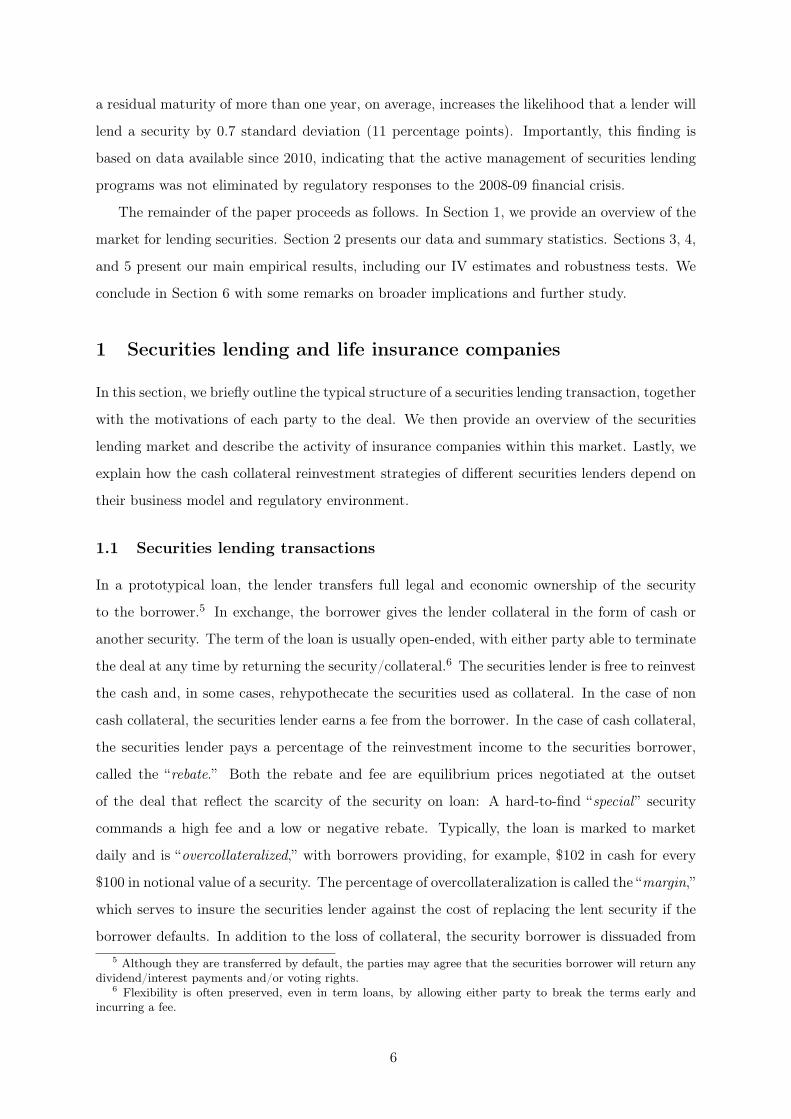
In a prototypical loan, the lender transfers full legal and economic ownership of the security
to the borrower.5 In exchange, the borrower gives the lender collateral in the form of cash or
another security. The term of the loan is usually open-ended, with either party able to terminate
the deal at any time by returning the security/collateral.6 The securities lender is free to reinvest
the cash and, in some cases, rehypothecate the securities used as collateral. In the case of non
cash collateral, the securities lender earns a fee from the borrower. In the case of cash collateral,
the securities lender pays a percentage of the reinvestment income to the securities borrower,
called the “rebate.” Both the rebate and fee are equilibrium prices negotiated at the outset
of the deal that reflect the scarcity of the security on loan: A hard-to-find “special ” security
commands a high fee and a low or negative rebate. Typically, the loan is marked to market
daily and is “overcollateralized,” with borrowers providing, for example, $102 in cash for every
$100 in notional value of a security. The percentage of overcollateralization is called the “margin,”
which serves to insure the securities lender against the cost of replacing the lent security if the
borrower defaults. In addition to the loss of collateral, the security borrower is dissuaded from5 Although they are transferred by default, the parties may agree that the securities borrower will return any
dividend/interest payments and/or voting rights.6 Flexibility is often preserved, even in term loans, by allowing either party to break the terms early and
incurring a fee.
6

defaulting on the loan by reputational effects: lender–borrower relationships are formed through
repeated transactions. Overall, the structure of cash-collateralized securities lending is closely
related to a sale and repo transaction, in which the securities borrower is entering a reverse-repo
arrangement (Duffie 1996, Garbade 2006).
A securities lending transaction usually involves three or four parties. The ultimate owner
of the security is typically an institutional investor such as a pension fund, insurance company,
mutual fund, or sovereign wealth fund. Owners of large portfolios will often conduct their own
lending programs, while smaller owners execute their programs through agent lenders, such as
custodian banks or asset managers, that act as large warehouses for securities made available for
lending. The end users of the borrowed securities are typically dealers and hedge funds. These
security market participants generally use large financial institutions, for example, broker-dealers
and investment banks, as intermediaries that regularly search for securities and have established
relationships with lenders.
The ultimate owners decide which securities in their portfolios will be made available to lend
and how the cash collateral proceeds of their lending programs will be reinvested. When they
choose to employ agent lenders, the owners typically provide guidelines or specific instructions
for the type of lending transactions (for example, minimum fee criteria or hard-to-find securities
only) and for the reinvestment of cash collateral. In some cases, as we will discuss below, these
reinvestment strategies are subject to regulatory limits.
If agent lenders are involved, they execute owners’ instructions to lend particular securities
and reinvest cash collateral. Because agent lenders often receive the same securities from many
ultimate owners, they typically allocate borrowing requests to securities using an algorithm
that ensures no owner receives preferential treatment. The agents earn a share of the profits
associated with lending securities, including fees and/or reinvestment income after rebate. In
exchange, agents will customarily provide indemnification against the risk that the non-cash
collateral is insufficient to replace the lent securities if the borrower defaults. To be clear, this
indemnification does not protect the owner against the risk of losses associated with reinvesting
cash collateral.
The borrowing intermediary generally performs three functions as it matches end-user
requests for securities with lenders’ availability. First, the intermediary helps to assuage
securities lenders’ potential concerns about the credit quality of end users, which may be small
and weakly regulated. Second, by establishing relationships with lenders and borrowers, they
can lower search costs. In the case of broker-dealers, their securities lending intermediation is
often combined with prime brokerage to lower costs further. Third, the intermediary may assume
7
some liquidity risk by establishing open-ended loans with lenders, giving them the freedom to
recall the securities as needed, and extending term loans to end users so they can be sure their
short positions are covered. In exchange for these services, the borrowing intermediary receives
a payment from the end user.7
The end users have a variety of reasons for borrowing a particular security. The most
common motivations are to take a short position or to cover a naked short position (Duffie
1996, Keane 2013); to avoid a settlement/delivery failure (Musto et al. 2011), possibly as part
of market making activity; to combine one security with other securities as part of an arbitrage
trading strategy; to obtain collateral for use in other transactions (Dive et al. 2011); and to take
advantage of tax or regulatory arbitrage (Faulkner 2006). The details of these strategies are
often complex and we refer the reader to the reference list for further explanation.
1.2 The securities lending market
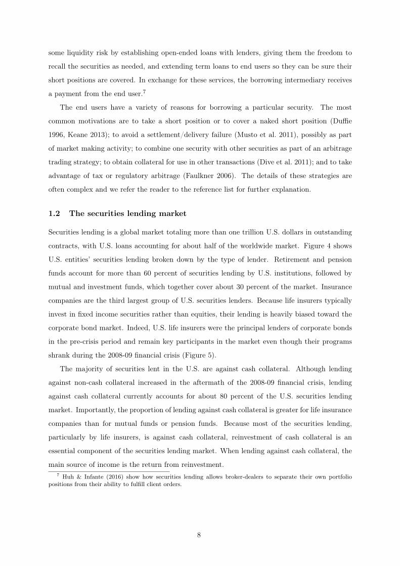
Securities lending is a global market totaling more than one trillion U.S. dollars in outstanding
contracts, with U.S. loans accounting for about half of the worldwide market. Figure 4 shows
U.S. entities’ securities lending broken down by the type of lender. Retirement and pension
funds account for more than 60 percent of securities lending by U.S. institutions, followed by
mutual and investment funds, which together cover about 30 percent of the market. Insurance
companies are the third largest group of U.S. securities lenders. Because life insurers typically
invest in fixed income securities rather than equities, their lending is heavily biased toward the
corporate bond market. Indeed, U.S. life insurers were the principal lenders of corporate bonds
in the pre-crisis period and remain key participants in the market even though their programs
shrank during the 2008-09 financial crisis (Figure 5).
The majority of securities lent in the U.S. are against cash collateral. Although lending
against non-cash collateral increased in the aftermath of the 2008-09 financial crisis, lending
against cash collateral currently accounts for about 80 percent of the U.S. securities lending
market. Importantly, the proportion of lending against cash collateral is greater for life insurance
companies than for mutual funds or pension funds. Because most of the securities lending,
particularly by life insurers, is against cash collateral, reinvestment of cash collateral is an
essential component of the securities lending market. When lending against cash collateral, the
main source of income is the return from reinvestment.7 Huh & Infante (2016) show how securities lending allows broker-dealers to separate their own portfolio
positions from their ability to fulfill client orders.
8
1.3 Securities lenders’ cash collateral reinvestment strategies
Regardless of their business model and regulatory environment, a financial institution can always
choose to pursue a passive cash collateral reinvestment strategy. In such cases, the securities
lender responds to borrowing requests and reinvests the cash collateral in safe assets of short
duration, for example in general collateral repo. The absence of maturity and liquidity mismatch
allows these programs to scale up or down with minimal concern for default by either party.
Alternatively, some financial institutions may choose an active cash collateral reinvestment
strategy. Such lenders aim to maintain a level of cash from securities borrowers to finance a
portfolio of longer-duration, higher-yielding assets, for example, corporate bonds, mortgages,
and mortgage-backed securities. Conditional on the size of their lending program, securities
lenders have the opportunity to increase the return from their lending programs by reinvesting
the cash collateral in riskier and/or longer-term assets. Because the term of the loan is usually
open-ended, this strategy creates a liquidity and/or maturity mismatch between the terms of
lending and reinvestment.
The degree to which a lending institution adopts an active reinvestment strategy depends
on its business model and regulatory environment. For example, mutual funds have essentially
no capital to absorb losses and their liabilities are mostly on demand. Their business model
encourages them to reinvest their cash collateral from securities lending in liquid asset, so
that they can return the cash collateral and receive back their lent securities upon demand.
Moreover, to protect mutual fund investors, the Securities and Exchange Commission (SEC)
subjects mutual funds’ reinvestment of cash collateral to the stringent SEC Rule 2a-7. According
to this rule, the weighted average maturity of cash reinvestment must be less than 60 days.8
Enforcement of this rule on mutual funds, together with other regulatory responses to the 2008-09
financial crisis, significantly shortened the maturity of reinvestment of cash collateral (Figure 6).
In contrast to mutual funds, other securities lenders traditionally have longer-term liabilities
and are subject to different regulations on the use of securities lending. For example, life
insurance companies and pension funds typically hold long-term contingent liabilities in the
form of insurance and pension contracts that are not used by consumers as protection against
illiquidity.9 Under their traditional business model, life insurers and pension funds match the
terms of their liabilities to those of safe and liquid assets. This model more easily allows life
insurers and pension funds to enhance the return on their asset portfolios because their liabilities8 In addition, Rule 2a-7 limits exposure to any counterparty to 5 percent, and requires mutual funds to hold
at least 10 percent of their cash reinvestment in daily liquid assets and at least 30 percent in weekly liquid assets.9 Health insurance companies and property and casualty life insurers are far less engaged in securities lending
because the terms of their liabilities are much shorter than life insurers or pension funds.
9
are not on demand. In addition, the regulatory rules on the use of securities lending are generally
weaker for life insurers and pension funds. This weaker regulatory environment exists despite the
NAIC adopting in 2010 more restrictive guidelines for state regulations pertaining to life insurers’
securities lending. The new guidelines stem from a review of securities lending practices at AIG
that contributed to its collapse during the 2008-09 financial crisis. In particular, the guidelines
specify that borrowers should post cash in the amount of at least 102 percent of domestic
securities borrowed (and at least 105 percent if the securities are foreign), that individual
loans should not be more than 5 percent of admitted assets, that cash reinvestment should
be “prudent,” and that all cash reinvestment securities (on- and off-balance sheet) are reported
in the NAIC Quarterly and Annual Statutory Filing Schedule DL.10
The differences in institutional business models and regulatory environments help determine
the scope of the cash reinvestment strategies of securities lenders. An institution with less liquid
liabilities and less stringent regulation on the use of securities lending may more easily enhance
the return on its portfolio by allowing greater maturity mismatch between the tenor of its
loans and the reinvestment of the cash collateral it receives.11 Currently, U.S. life insurers have
significantly greater maturity mismatch between their securities lending and their reinvestment
of cash collateral than the median securities lender (Figure 8). The mean U.S. life insurer
maturity mismatch (not shown) is about 1,000 days, compared with about 100 days for the
mean securities lender, shown by the blue line in Figure 6. Indeed, life insurers’ reinvestment of
cash collateral currently has an average maturity more than 15 times larger than the regulatory
maximum of mutual funds’ cash reinvestment.
That said, to better understand the securities lending strategies of pension funds and life
insurance companies requires detailed data on individual loans and cash reinvestment decisions.
In the case of pension funds, these data are not available. Although some funds report aggregate
level information on their portfolio holdings and lending programs, crucial data are missing on
their individual security loan decisions and their cash reinvestment strategies.
By contrast, state insurance regulators’ adoption of the NAIC guidelines for enhanced
reporting on securities lending programs presents a golden opportunity to observe new and
detailed information about securities lending and cash reinvestment activities by U.S. life
insurers. We can observe the individual securities that are lent by life insurers, the maturity10 In addition, each asset financed with cash collateral recorded in the NAIC Quarterly and Annual Statutory
Filing Schedule D attracts a risk-based capital charge consistent with its NAIC designation code.http://www.dfs.ny.gov/insurance/circltr/2010/cl2010_16.htmhttp://www.naic.org/capital_markets_archive/110708.htm
11 Regulatory arbitrage as a source of reach for yield has already been documented in the U.S. life insuranceindustry through the deliberate portfolio selection of more risky corporate bonds within a rating class (Becker& Ivashina 2015), the use of captive reinsurers to lower regulatory capital charges (Koijen & Yogo forthcoming),and the issuance of institutional funding agreements (Foley-Fisher et al. 2015).
10
of the collateral they received, and their cash reinvestment portfolios. When combined with
security-level data on the broader securities lending market, we can deepen our understanding
of the strategic use of securities lending by U.S. life insurers to raise the return on their
portfolio of assets. To be sure, we do not have data on the maturity structure of life insurers’
reinvestment of cash collateral before 2010 and, thus, cannot gauge how their reinvestment
strategy changed following the 2008-09 financial crisis and in response to the new regulatory
environment. Nevertheless, these new data offer the best possible insight into the ongoing
strategies pursued by institutions whose business models and regulatory environment are similar
to life insurers’, including, for example, pension funds. In the next section, we describe how we
put the data together.
2 Data
We combine several data sources to obtain the dataset we use in our analysis. The data on
insurance company holdings and securities lending activity come from the NAIC Quarterly
and Annual Statutory Filings.12 Within these filings, Schedule DL is a relatively new report of
individual investments made by life insurers using cash collateral received from securities lending,
both on- and off-balance sheets. The Schedule DL was introduced in 2010 as one of many changes
to the reporting and statutory accounting of securities lending transactions adopted as a response
to the 2008-09 financial crisis. In general, the new data allow us to better track the securities
lending transactions entered into by an insurer and to observe detailed information about the
life insurers’ use of the collateral received. For example, from 2010, if the collateral received from
securities lending could “be sold or pledged by custom or contract by the reporting entity or its
agent,” then the reinvested collateral should be recorded on the balance sheet.13 We hand-coded
data about the maturity of the collateral received in the securities lending transactions from the
regulatory Notes to the Financial Statements. Figure 7 shows that the total amount of securities
lending by U.S. life insurers reached over $55 billion at the end of 2013. Because we rely on the
detailed information contained in Schedule DL as part of the new reporting requirements, our
sample by necessity begins in 2010.
The NAIC Quarterly and Annual Statutory Filings also contain Schedule D, reporting life
insurers’ individual fixed income holdings at year-end, together with cross-sectional information
about each security, including the CUSIP indentifier, the NAIC designation code, and whether12 Historical NAIC Quarterly and Annual Statutory Filings are contained in the NAIC Financial Data
Repository, a centralized warehouse of financial data used primarily by state and federal regulators.13 Amendments to SSAP No. 91-R, Accounting for Transfers and Servicing of Financial Assets and
Extinguishments of Liabilities.
11

the bond was on loan as part of the insurer’s securities lending program. We drew information
about the total size and performance of the life insurer’s investment portfolio from the summary
balance sheet contained in the NAIC Quarterly and Annual Statutory Filings. We focus on
all insurance companies that had a securities lending program at any point during our sample
period. Our baseline dataset includes information on 107 life insurers, with holdings data on
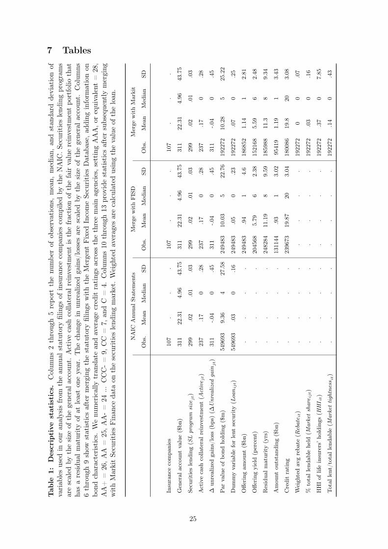
over half a million bonds. The first four columns of Table 1 report descriptive statistics for the
baseline sample. The average bond holding is about $9 million with a standard deviation of
$27.6 million. The dummy variable for securities lending indicates that about 3 percent of the
bond holdings were lent at some point during the period.
We obtain bond characteristics from Mergent FISD and add them to our baseline dataset.
FISD provides a wide range of security-level information for mostly U.S. corporate, agency, and
government bonds that can be merged with our holdings data using the CUSIP identifier. Our
focus on life insurers’ holdings and lending of corporate bonds is consistent with their strong
bias toward this sector of the securities lending market, as described in Section 1. Including this
additional information reduces our bond holdings data to about 250,000 bond holdings across
the same set of 107 life insurers. Columns 5 through 8 of Table 1 report the additional descriptive
statistics, including amount issued, offering yield, credit rating, and residual maturity. In this
merged sample, the average offering amount of the bonds held is $10 million (with a standard
deviation of $22.8 million), with a yield of about 6 percent. The average residual maturity
across all year-end bond holdings is 11.2 years (with a standard deviation of 9.6 years). Our
numerical rating measure indicates that the average is about 20, equivalent to a Standard &
Poor’s bond rating of BBB.14 Lastly, the average total amount outstanding across all bonds held
by life insurers is $900 million.
Markit Securities Finance provides information on individual securities lending transactions.
This dataset offers the most comprehensive view of the securities lending market, covering about
85 percent of the global market and more than 90 percent of the U.S. securities lending market.
The daily transaction level data include identifiers of the lent security, such as CUSIP and ISIN;
value, quantity and tenure of the loan; the relevant rates, such as securities lending fee and rebate
rate; and the type of collateral (cash or non-cash). For each lent security, the total value and
quantity of the inventory available to lend is also reported. We cannot observe counterparties
to individual loans, nor information on lenders’ reinvestment of cash collateral. We construct
weighted averages of the available variables, for each security, across all transactions conducted14 We collect data on ratings from Moody’s, Fitch, and Standard & Poor’s and combine them into a single
rating using the lowest rating when only two are available and the median rating when all three are available.To average the ratings, we set AAA, or equivalent = 28, AA+ = 26, AA = 25, AA- = 24 ... CCC- = 9, CC =7, and C = 4.
12

during the 14 days around year-end. Our final dataset contains data for 107 life insurers and over
187,000 bond holdings.15 Columns 9 through 12 of Table 1 report the descriptive statistics for
the dataset following this merge. The information from the securities lending market suggests
that the weighted average rebate on the bonds is about zero. On average, life insurers hold about
3 percent of each security’s total lendable amount (with a standard deviation of 16 percent),
with a concentration of holdings index (HHI) value equal to 0.37. Lastly, our measure of each
security’s market tightness, defined as the ratio of the total amount lent to the total amount
that is lendable, indicates that, on average, about 14 percent of the available amount of each
security is actually lent. The remaining entries in these columns show that the other observable
characteristics of the bond holdings do not vary significantly between the baseline and merged
datasets.
Taken together, these data offer a new lens through which we can obtain a comprehensive and
detailed view of all aspects of the life insurers’ securities lending programs, from the individual
bonds lent, through the collateral received, to the reinvestment portfolios. As a simple analysis
of the kinds of bonds that life insurers are lending, Table 2 compares descriptive statistics of
securities used in lending transactions compared with the securities not lent.16 In general, the
securities that life insurers tend to lend have a slightly larger par value and have a longer residual
maturity in comparison with the rest of their portfolio. Life insurers also tend to lend securities
with a lower rebate (higher fee) and in which there is a greater concentration of holding and
market tightness. Of course, these pairwise comparisons of mean characteristics are indicative.
In the following three sections, we provide a more careful empirical analysis of securities
lending by U.S. life insurers. First, we explore the bond and market characteristics that
determine an insurer’s decision to lend individual securities. Second, we show how fundamental
endogeneity concerns preclude finding compelling evidence for active securities lending within
an insurer. And third, we present our methodology for showing that active management of the
portfolio plays a significant role in the overall strategy for the lending program.
3 Determinants of securities lending by U.S. life insurers
Our first set of empirical tests investigates the relationship between a life insurer’s decision to lend
a particular bond and its market share in that bond. We assume that life insurers are endowed
with a portfolio of securities over which they can make lending decisions. This assumption is15 There are 1,029 out of 14,149 securities reported by life insurers as on loan, but for which no securities
lending information is available in Markit; we exclude these observations from our analysis.16 The table counts each security holding as a separate observation, effectively weighting the descriptive
statistics by the number of times that a security is lent or not.
13

in keeping with industry practice, where the agents who manage the securities lending portfolio
are not those who decide the broad investment strategy or specific asset purchases. We denote
by Loanijt a binary variable that takes a value of 1 if insurer j is loaning bond i at year t, and
0 otherwise. The main explanatory variable (Market shareijt) is the year-t holding by insurer j
in bond i as a share of the total amount of bond i that is made available to securities borrowers
by all lenders. We specify a linear model:
Loanijt = α1i + α2
j + α3t + βMarket shareijt +Zitγ + εijt , (1)
where Zit is a matrix of bond-specific time-varying characteristics. The set of α fixed effects
captures unobservable heterogeneity across securities, life insurers, and time.
Table 3 summarizes the results. Column 1 shows the baseline model, controlling for insurer,
year, and bond issuer fixed effects. The association between Loanijt and Market shareijt
is positive and statistically significant at less than the 1 percent level. The coefficient on
Market shareijt suggests that, on average, a one standard deviation (13.4 percent) increase
in an insurer’s market share in a particular bond is associated with a 0.6 percent increase in the
probability that the bond is loaned.
The remaining columns of Table 3 investigate the robustness of this association to additional
security- and market-level controls that are likely to be correlated with the demand for individual
bonds. Column 2 of Table 3 controls for bond characteristics, including the residual maturity,
offering yield, offering amount, amount outstanding, and credit rating. Including these finer
controls reduces the original sample by about 60 percent. Nevertheless, the association between
the probability that an insurer loans a bond and the market share remains largely unchanged.
Furthermore, the coefficient estimate on the offering yield and rating are negative, and the
coefficient estimate on residual maturity is positive. These findings are broadly consistent with
previous empirical studies, for example, Asquith, Au, Covert & Pathak (2013).
Column 3 of Table 3 controls for loan market tightness (Market tightness it), defined as the
fraction of a bond that is on loan relative to the total amount of that bond that is made available
for loan by all lenders, and the bond rebate (Rebateit). The inclusion of Market tightness it
and Rebateit has little effect on the magnitude and significance of the coefficient estimate on
Market shareijt. In addition, consistent with Kolasinski et al. (2013), the estimates suggest that,
when controlling for overall market tightness and an insurer’s market share in that bond, there
is a significant positive association between a more special bond—i.e. a more negative rebate—
and the probability that the bond will be on loan. Column 4 of Table 3 adds a measure of
concentration for individual securities in the life insurance industry (HHI it) using the Herfindahl–
14

Hirschman Index computed at the bond-year level using only life insurers’ market shares in each
individual bond.17
This new finding that life insurers are more likely to lend securities in which they have a
greater market share is consistent with the existing empirical literature that studies the passive
lending channel (Kolasinski et al. 2013, Kaplan et al. 2013) and those theories emphasizing search
frictions (Miller 1977, Duffie et al. 2002, Vayanos & Weill 2008). Intuitively, the probability of
loaning a bond is higher if a securities borrower is matched with a lender with a high market
share in that bond. Knowing that they face a greater opportunity cost in looking elsewhere for
the bond, the match is more likely to be consummated.
However, the finding is also consistent with the active lending channel. In such a case, a
lender would be more likely to lend bonds in which it has a high market share. The lender knows
it can more easily finance a portfolio of long-dated assets and earn a spread between the cost of
cash borrowing and the return on these assets.18
4 Endogeneity of the cost of cash from securities lending
We build on the analysis of the previous section to understand the major endogeneity challenge
in identifying the active lending channel through the lending decisions of a single lender. First,
lenders may be able to control factors that affect the borrowing decision, such as the terms of the
loan. Second, those factors and/or the lender’s ability to control them may be correlated with
the lender’s strategy. Consider, for example, the previous regression specification representing
the loan decision in conjunction with a specification that represents the equilibrium rebate:
Loanijt = α1i + α2
j + α3t + βMarket shareijt + δRebateit +Zijtγ + εijt (2)
Rebateit = α̃1i + α̃3
t + Z̃ijtγ̃ + ε̃ijt . (3)
As is widely known, if any variable (Z̃ijt) in equation 3 that determines the equilibrium rebate
is omitted from the loan decision specification, all the coefficient estimates from equation 2 will
be inconsistent (Greene 2012).
We can demonstrate that confounding factors are likely to be a serious concern by estimating17 The calculation is limited by our ability to observe only the holdings in our data–i.e., by necessity, it assumes
atomistic holdings by other institutions.18 The statistically significant negative coefficient on HHI it is also consistent with both an active and passive
securities lending strategy. With passive lenders, an increase in bond concentration reduces the probability thata borrower seeking a bond is matched with an insurer holding that bond, which decreases the probability of theloan. With active lenders, an increase in concentration implies that the value of the rebate on that bond rises–i.e.,the bond becomes less special–as more of the bond is supplied to securities borrowers. As the bond becomes lessscarce and the rebate increases, the cost of borrowing cash by lending that bond also increases, which reducesthe likelihood of loaning the bond.
15

equation 3 using known variables from equation 2. Because known variables are correlated with
a bond’s rebate, it is likely that other (potentially unobservable) determinants of the lending
decision are also correlated with the bond’s rebate. We show that the rebate is a function of the
concentration of holdings in that bond. Intuitively, lenders of hard-to-find securities can get a
better deal on their transaction—as in Duffie (1996)—and this may affect their decision to lend
particular securities.
We first show that the cost of raising cash by lending a particular security is a function of
life insurers’ holdings of that security. Adding weight to this likely source of endogeneity, we
also show that life insurers may affect the shadow value of their entire lending program. We
aggregate the lending decisions over segments of life insurers’ bond portfolios and show there is
a positive association between the decision to lend bonds within that segment and the holdings
distribution of that segment. Taken together, the results suggest that a life insurer may be able
to control the cost of cash that it can raise by choosing which bonds to lend, and this confounds
the identification of active securities lending. The implication is that we cannot use correlates
of the loan decisions within a life insurer to establish the presence of an active securities lending
channel.
4.1 Determinants of the rebate on a bond
Table 4 summarizes the results from investigating the relationship between a bond’s rebate and
the concentration of that bond’s holdings across life insurers. As described in Section 1, a hard-
to-find security attracts a lower and sometimes negative rebate. To be clear, in the latter case,
the security borrower pays a premium to the lender in excess of the return from reinvesting the
cash collateral. Our specifications are based on equation 3, with the unit of observation being a
bond i held by insurer j at the end of year t. We restrict the sample to bonds that have at least
three holders in any given year to obtain meaningful variation in the distribution of holdings.
The coefficient on HHI it suggests that those bonds that are the most concentrated among
life insurers tend to have a lower rebate (that is, tend to be more special). Column 1 of Table 4
reports the result of a regression of Rebateit on HHI it. This baseline specification includes the
loan decision, life insurer, year, and bond issuer fixed effects. Column 2 adds market share,
market tightness, and other bond-level controls to the specification.19 Columns 3 and 4 separate
the sample into those bonds that are on loan and those that are not loaned by any life insurer,
respectively. In all cases, the relationship between Rebateit and HHI it is statistically significant
at less than the 1 percent level. The baseline coefficient estimate suggests that, on average,19 In general, we find results that are qualitatively similar to those of Nashikkar & Pedersen (2007).
16

a one standard deviation increase in a bond concentration is associated with a 0.4 percentage
point (1.2 standard deviation) decrease in the rebate rate for that security.20
Taken together, the results reported in Table 4 show the likely endogenity of bond rebates
and loan decisions. Although a bond’s rebate is likely to be a function of the size of life insurers’
holdings, life insurers’ decisions to lend the bond are likely to be influenced by its specialness.
More generally, the findings support a concern that life insurers may be able to use their market
power over a large number of bonds to exert significant control over their cost of cash borrowing
via securities lending. This means that, unless the regression that specifies the loan decision
accounts for all the co-determinants of a bond’s rebate, the coefficient estimates from equation 2
will be inconsistent.
4.2 Determinants of an insurer’s overall cost of cash collateral
We now study the potential endogeneity of life insurers’ overall cost of raising cash collateral via
securities lending. The previous section provided some evidence that individual bond specialness
is potentially determined by the distribution of bond holdings and by life insurers’ decisions to
lend. The findings, however, are only suggestive of an insurer’s ability to exert control over
its overall cost of funding. For example, life insurers may have market power for only a small
fraction of their portfolio. Although an insurer might exert control over the rebate on some
bonds, its control over the rebate on other bonds could be more limited.
To assess the determinants of life insurers’ overall cost of funding requires summarizing the
content of their portfolios. A crude approach is to run the same test as in Table 4 using averages
of the previously defined variables calculated over each insurer’s portfolio. However, aggregating
bond-level information to the insurer level is likely to produce a test without much power. We
adopt an alternative approach by creating subsets of life insurers’ bond portfolios. Specifically,
we rank each life insurer’s bond portfolio according to the rebate of each bond and divide the
portfolios according to rebate quantiles, which yields equal-sized groups of bonds that differ by
the average rebate of the bonds in each group. Then, for each equal-sized bond group within
two rebate quantiles, we compute a weighted average analog of the variables discussed in the
previous sections. Throughout the analysis, the weights are the shares of a bond in terms of the
fair value with respect to the total fair value of the bonds in the group. The unit of observation
for this analysis is a rebate group q for bonds held by a life insurer j at the end of year t. With20 The positive association between Rebateit and Loanijt, conditional on HHI it, is consistent with both a
passive and active securities lending program. When life insurers are passive, a bond that is more sought aftershould attract a higher rebate in order to secure the loan, resulting in a positive association between the lendingdecision and the rebate. Conversely, active life insurers may choose to lend a bond for which they receive a betterdeal—a more negative rebate—to minimize their overall cost of cash borrowing, resulting in the same correlation.
17

variables defined as before, the regression specification is:
Loanqjt = α1q + α2
j + α3t + βMarket shareqjt +Zqjtγ + εqjt . (4)
Columns 1 and 4 of Table 5 summarize the regression results for 32 and 64 rebate groups,
respectively. These specifications control for weighted average bond characteristics in each group,
as well as insurer and year fixed effects. The coefficient estimates suggest there is a positive and
robust association between the fraction of bonds on loan and the weighted average market share
in those bonds, conditional on the weighted average rebate and concentration. Columns 2 and 3
perform the same test on the subsets of 32 rebate groups above and below the median rebate,
respectively. The coefficient on Market shareqjt is broadly similar, with marginally weaker
significance for rebate groups below the median rebate. Columns 5 and 6 repeat this test
on the subsets of 64 rebate groups above and below the median rebate, respectively. Here, the
coefficient on Market shareqjt is only significant for the sample of groups above the median,
suggesting that the positive association between the loan and market share is likely to be more
pronounced in the portion of the portfolio that has a higher average rebate. However, since a
higher rebate tends to be associated with a higher probability of loaning a bond, increasing the
number of quantiles mechanically reduces the fraction of loaned bonds in the lower group. As a
result, any correlation between average loan and market share is likely to be weaker.
Taken together, these results suggest that the association between the fraction of bonds
loaned and the weighted average market share is significant in a large portion of life insurers’
bond portfolios–at least half of the bonds–and especially so in the portion of the portfolio above
the median rebate rate. We interpret this result as suggesting that life insurers are likely to have
significant control over their overall cost of funding via securities lending.
The analysis presented in this section suggests that an analysis of the loan decisions of a
single insurer is unlikely to provide compelling evidence for an active lending channel. We find
support for the argument that there are factors affecting the securities borrowing decisions that
may be influenced by lenders themselves. We can and do control for the obvious candidates in
our analysis reported in Section 3, but the list of potential confounding factors is practically
endless.
5 Securities lending as wholesale funding
To build a compelling case that there is an active securities lending channel, we adopt a two-
fold strategy. First, we exploit the ability to observe in our data the same bonds at the
18

same time across different life insurers’ portfolios. We introduce security–time fixed effects
to control for potentially confounding factors in a reduced form that encompasses the cost of
cash borrowing, as well as the availability and distribution of holdings, associated with each
security. Second, we propose an instrumental variable to deal with possibly unobservable time-
varying insurer heterogeneity. Our two-step approach is intended to approximate the theoretical
ideal experiment to establish an active lending channel: testing whether two life insurers with
identical bond portfolios would make differentl lending decisions if one exogenously engaged in
greater maturity mismatch.
5.1 Controlling for bond-specific factors
Our proxy for the extent of active management (Activejt) is the fraction of assets in the cash
reinvestment portfolio of a life insurer j at year t that has a residual maturity of more than
one year. This threshold captures investment in assets that are ineligible for purchase by MMFs
under Rule 2a-7 and are therefore likely to offer a higher return than cash instruments.21 As
is clear from Figure 8, there is variation in this fraction across life insurers and over time. We
include Activejt as the main explanatory variable in a linear specification that includes security–
time and life insurer fixed effects:
Loanijt = α1i + α2
j + α3t + α1
i × α3t + βActivejt + εijt . (5)
Under a passive lending strategy, Activejt would be uncorrelated with Lend ijt, that is, β = 0.
By contrast, in the presence of an active lending strategy, the proxy would be associated with a
greater likelihood that a bond will be loaned.
Columns 1 and 2 of Table 6 report the results of estimating equation 5 with only life insurer
fixed effects and then including security–time fixed effects, respectively.22 The coefficient on
Activejt suggests that, on average, a one standard deviation increase in the fraction of a life
insurer’s cash reinvestment portfolio invested in assets with maturities greater than 1 year is
associated with a 2 percent increase in the probability that the bond is loaned. This association
is significant at less than the 1 percent level.21 By way of further comparison, this threshold is six times the regulatory limit on mutual fund cash
reinvestment.22 The number of observations is much larger than in sections 3 and 4 because the sample is no longer restricted
by the availability of rebate information.
19

5.2 Controlling for insurer-specific unobservable heterogeneity
The variable Activejt may itself be endogenous. The residual error term εijt in equation 5
may contain unobservable insurer-specific time-varying factors that are correlated with Activejt.
Although we can control for bond-specific, time-varying unobservable factors through the
interacted fixed effects, we cannot control for all time-varying insurer heterogeneity that affects
its ability to lend bonds. For example, life insurers may have bundles of bonds that facilitate
lending only in some years.
To obtain exogenous variation in the degree of active cash collateral reinvestment by an
insurer (Activejt), we introduce, as an instrumental variable, the annual change in the amount
of unrealized gains/losses on the life insurer’s bond portfolio as a fraction of that insurer’s
total assets (∆Unrealized gainjt). Under statutory accounting rules, an insurance company
must report the current market value of the securities in its portfolios. Life insurers calculate
the unrealized gain/loss as the difference between the cost of its portfolio and the current
liquidation value. The unrealized gain/loss on a portfolio is incorporated into ratings agencies’
evaluations of the financial strength of an insurer, because they can predict actual economic losses
(Standard and Poor’s 2009). Our strategy is predicated on the idea that an active securities
lender will attempt to compensate for the change in unrealized losses on its underlying portfolio
by increasing the return on its cash reinvestment portfolio. Unrealized losses are themselves
plausibly beyond the control of the manager of an insurer’s securities lending program and,
therefore, from the unobserved heterogeneity that is the source of the endogeneity concern.
Columns 3 and 4 of Table 6 report the first- and second-stage results of a regression of
Loanijt on Activejt, instrumenting Activejt with ∆Unrealized gainjt. As with the reduced form
in Column 2 of Table 6, the IV regression includes CUSIP, CUSIP–year, and insurer fixed effects.
Column 3 of Table 6 shows that there is a positive first-stage association between Activejt and
∆Unrealized gainjt. The coefficient on Activejt in Column 4 of Table 6 suggests that, on average,
a one standard deviation increase in the fraction of an insurer’s cash reinvestment portfolio
invested in assets with maturities greater than 1 year is associated with an 11% increase in the
probability that the bond is loaned.23
The parameter estimates imply there would be only a small reduction in lending if Rule
2a-7 limits were imposed on the securities lending programs of U.S. life insurance companies.
Table 1 shows that life insurers in our post-crisis sample have on average about 17 percent of
their cash collateral portfolio reinvested in bonds with a residual maturity of at least one year.23 We suspect that our IV coefficient is larger than our OLS coefficient because our empirical approach places
greater weight on life insurers that have more variation in active reinvestment over time (Angrist, Graddy &Imbens 2000).
20
Rule 2a-7 would remove these bonds entirely from the portfolio.24 Using the coefficient estimate
from Table 6 of the effect of Activejt on the probability of lending (0.4), elimination of the active
lending channel would reduce lending by 0.4×0.17, which is about 7 percent. Figure 7 shows that
life insurers’ lending against cash collateral amounts to about $55 billion, indicating a potential
decline in the market of 0.07×$55 billion, or less than $4 billion. This crude calculation suggests
that regulation equivalent to Rule 2a-7 on cash collateral reinvestment by life insurers could
enhance financial stability with only minor consequences for bond market functioning.
5.3 Robustness
Table 7 summarizes tests of the robustness of the association between the decision to lend
securities and the degree of active cash collateral reinvestment. One concern is that variation in
the size of an insurer’s securities lending program over time may be driving the result. Columns 1
and 2 report the instrumental variable results including as a control the size of the insurer’s
securities lending program (SL program sizejt). A further concern is that life insurers may have
a preference for lending particular securities. Columns 3 and 4 report the results of repeating
the analysis including CUSIP–insurer fixed effects. The estimated coefficient of interest in both
cases is similar to our previous results.
6 Conclusion
This paper offers the first empirical evidence that certain financial insitutions use securities
lending as a source of wholesale funding. That is, some firms raise and maintain a level of cash
collateral by lending lower-yielding securities and investing the proceeds in longer-term higher-
yielding securities. Our main empirical exercise shows that U.S. life insurers’ lending decisions
are driven in part by the degree of maturity mismatch in their securities lending programs.
We acknowledge and address the stringent identification challenge posed by securities lenders’
potential ability to influence unobservable factors that affect the borrowing decision. The finding
stands in contrast to the widespread perception in the existing literature that securities lenders
passively respond to borrower demands and reinvest their cash collateral in short-term funding
markets.
Our evidence based on data from the period after the implementation of sweeping
macro- and microprudential reforms that followed the 2008-09 financial crisis demonstrates
the vulnerabilities that securities lenders still pose to securities market functioning. A sharp24 In addition to restricting the weighted average maturity of the reinvestment portfolio to less than 60 days,
Rule 2a-7 specifies that mutual funds can only invest in non-MMF eligible securities with an exception from theSEC. MMF eligible securities must have a residual maturity of less than 13 months.
21
contraction in repo funding from securities lenders is one way a run on active securities lenders
can adversely affect securities markets, as discussed in the introduction and emphasized by
Brunnermeier & Pedersen (2009) and Gorton & Metrick (2010a,b). In addition, during times
of financial distress, concerns about securities lenders’ cash reinvestment portfolios may require
borrowers to post larger margins to compensate broker-dealers for the risk to their cash. In
both cases, the underlying vulnerability to runs from liquidity and/or maturity mismatch can
be attributed to the active lending channel. One possible reason that life insurers remain active
securities lenders is the persistent low interest rate environment. Low returns to institutional
investors’ portfolios deriving from a long period of low interest rates increase their incentive to
actively manage their securities lending programs.
In light of these vulnerabilities, measures such as the degree of maturity mismatch and the
extent to which active securities lenders provide tri-party repo funding are important financial
stability metrics. Careful monitoring of securities lenders’ programs is especially important
for the functioning of corporate bond markets, where financial stability concerns are greatest.
Although these measures are available to some extent in the regulatory filings of U.S. life insurers,
they are not widely available for all securities lenders.25
References
Adrian, T., Begalle, B., Copeland, A. & Martin, A. (2012), ‘Repo and Securities Lending’,
National Bureau of Economic Research Working Paper No. 18549 .
Angrist, J., Graddy, K. & Imbens, G. (2000), ‘The interpretation of instrumental variables
estimators in simultaneous equations models with an application to the demand for fish’,
Review of Economic Studies 67(3), 499–527.
Asquith, P., Au, A. S., Covert, T. & Pathak, P. A. (2013), ‘The market for borrowing corporate
bonds’, Journal of Financial Economics 107(1), 155–182.
Becker, B. & Ivashina, V. (2015), ‘Reaching for yield in the bond market’, The Journal of
Finance 70(5), 1863–1902.
Brunnermeier, M. K. & Pedersen, L. H. (2009), ‘Market liquidity and funding liquidity’, Review
of Financial Studies 22(6), 2201–2238.25 Measures of maturity mismatch and repo funding associated with securities lending programs would augment
the data collection proposed by Adrian, Begalle, Copeland & Martin (2012). Koijen & Yogo (2015) note that lifeinsurers’ statutory filings lack details on the international dimensions of life insurers’ securities lending programs.
22

Covitz, D., Liang, N. & Suarez, G. A. (2013), ‘The evolution of a financial crisis: Collapse of
the asset-backed commercial paper market’, The Journal of Finance 68(3), 815–848.
Diamond, D. W. & Dybvig, P. H. (1983), ‘Bank Runs, Deposit Insurance, and Liquidity’, The
Journal of Political Economy 91(3), 401–419.
Dive, M., Hodge, R., Jones, C. & Purchase, J. (2011), ‘Developments in the global securities
lending market’, Bank of England Quarterly Bulletin .
Duffie, D. (1996), ‘Special repo rates’, The Journal of Finance 51(2), 493–526.
Duffie, D., Gârleanu, N. & Pedersen, L. H. (2002), ‘Securities lending, shorting, and pricing’,
Journal of Financial Economics 66(2), 307–339.
Faulkner, M. (2006), An Introduction to Securities Lending, London: Spitalfields Advisors.
Foley-Fisher, N., Narajabad, B. & Verani, S. (2015), ‘Self-fulfilling Runs: Evidence from the
U.S. Life Insurance Industry’, Finance and Economics Discussion Paper Series 2015-032 .
Garbade, K. (2006), ‘The evolution of repo contracting conventions in the 1980s’, Economic
Policy Review 12(1).
Goldstein, I. & Pauzner, A. (2005), ‘Demand–deposit contracts and the probability of bank
runs’, the Journal of Finance 60(3), 1293–1327.
Gorton, G. & Metrick, A. (2010a), ‘Haircuts’, Federal Reserve Bank of St. Louis Review
(Nov), 507–520.
Gorton, G. & Metrick, A. (2010b), ‘Regulating the shadow banking system’, Brookings Papers
on Economic Activity pp. 261–312.
Gorton, G. & Metrick, A. (2012), ‘Securitized banking and the run on repo’, Journal of Financial
Economics 104(3), 425 – 451.
Greene, W. (2012), Econometric Analysis (7th Edition), Pearson Education.
He, Z. & Xiong, W. (2012), ‘Dynamic debt runs’, Review of Financial Studies 25(6), 1799–1843.
Huh, Y. & Infante, S. (2016), ‘Bond Market Liquidity and the Role of Repo’, mimeo .
Kaplan, S. N., Moskowitz, T. J. & Sensoy, B. A. (2013), ‘The effects of stock lending on security
prices: An experiment’, The Journal of Finance 68(5), 1891–1936.
23

Keane, F. M. (2013), ‘Securities loans collateralized by cash: Reinvestment risk, run risk, and
incentive issues’, Current Issues in Economics and Finance 19(3).
Koijen, R. S. & Yogo, M. (2015), ‘Risks of Life Insurers: Recent Trends and Transmission
Mechanisms’, mimeo .
Koijen, R. S. & Yogo, M. (forthcoming), ‘Shadow Insurance’, Econometrica .
Kolasinski, A. C., Reed, A. V. & Ringgenberg, M. C. (2013), ‘A multiple lender approach
to understanding supply and search in the equity lending market’, The Journal of Finance
68(2), 559–595.
Krishnamurthy, A., Nagel, S. & Orlov, D. (2014), ‘Sizing up repo’, The Journal of Finance
69(6), 2381–2417.
McDonald, R. & Paulson, A. (2015), ‘AIG in Hindsight’, Journal of Economic Perspectives
29(2), 81–105.
Miller, E. M. (1977), ‘Risk, uncertainty, and divergence of opinion’, The Journal of Finance
32(4), 1151–1168.
Musto, D., Nini, G. & Schwarz, K. (2011), ‘Notes on bonds: Liquidity at all costs in the great
recession’, mimeo .
Nashikkar, A. J. & Pedersen, L. H. (2007), ‘Corporate Bond Specialness’, mimeo .
Peirce, H. (2014), ‘Securities Lending and the Untold Story in the Collapse of AIG’, George
Mason University Mercatus Center Working Paper No. 14-12 .
Schmidt, L., Timmerman, A. & Wermers, R. (forthcoming), ‘Runs on money market mutual
funds’, American Economic Review .
Schroth, E., Suarez, G. A. & Taylor, L. A. (2014), ‘Dynamic debt runs and financial fragility:
Evidence from the 2007 ABCP crisis’, Journal of Financial Economics 112(2), 164–189.
Standard and Poor’s (2009), ‘Methodology And Assumptions For Gauging The Impact Of
Unrealized Losses On Insurers’ Financial Strength’.
Vayanos, D. & Weill, P. (2008), ‘A search-based theory of the on-the-run phenomenon’, The
Journal of Finance 63(3), 1361–1398.
24
7 TablesTab
le1:
Des
crip
tive
stat
isti
cs.
Colum
ns2throug
h5repo
rtthenu
mbe
rof
observations,mean,
med
ian,
andstan
dard
deviationof
variab
lesused
inou
ran
alysis
from
thean
nual
statutoryfilings
ofinsuranc
ecompa
nies
compiledby
theNAIC
.Se
curities
lend
ingprog
rams
arescaled
bythesize
ofthegenerala
ccou
nt.Activecash
colla
teralr
einv
estm
entis
thefraction
ofthefair
valuereinvestmentpo
rtfolio
that
hasaresidu
almaturityof
atleaston
eyear.The
chan
gein
unrealized
gains/losses
arescaled
bythesize
ofthegene
ralaccoun
t.Colum
ns6throug
h9show
statistics
aftermerging
thestatutoryfilings
withtheMergent
Fixed
IncomeSe
curities
Datab
ase,
adding
inform
ationon
bond
characteristics.
Wenu
merically
tran
slatean
daverag
ecred
itrating
sacross
thethreemainag
encies,settingAAA,o
requivalent
=28
,AA+
=26
,AA
=25
,AA-=
24...
CCC-=
9,CC
=7,
andC
=4.
Colum
ns10
throug
h13
providestatistics
aftersubseque
ntly
merging
withMarkitSecurities
Finan
ceda
taon
thesecu
rities
lend
ingmarket.
Weigh
tedaverag
esarecalculated
usingthevalueof
theloan
.
NAIC
Ann
ualS
tatements
Merge
withFISD
Merge
withMarkit
Obs.
Mean
Med
ian
SDObs.
Mean
Med
ian
SDObs.
Mean
Med
ian
SD
Insurancecompa
nies
107
..
.107
..
.107
..
.
Gen
eral
accoun
tvalue($bn
)311
22.31
4.96
43.75
311
22.31
4.96
43.75
311
22.31
4.96
43.75
Securities
lend
ing(S
Lpr
ogra
msi
zejt)
299
.02
.01
.03
299
.02
.01
.03
299
.02
.01
.03
Activecash
colla
teralr
einv
estm
ent(A
ctiv
e jt)
237
.17
0.28
237
.17
0.28
237
.17
0.28
∆un
realized
gains/loss
(bps)(∆
Unr
ealiz
edga
injt)
311
-.04
0.45
311
-.04
0.45
311
-.04
0.45
Par
valueof
bond
holding($m)
549693
9.36
427.58
249483
10.03
522.76
192272
10.28
525.22
Dum
myvariab
leforlent
security
(Loa
nij
t)
549693
.03
0.16
249483
.05
0.23
192272
.07
0.25
Offe
ring
amou
nt($bn
).
..
.249483
.94
14.6
186852
1.14
12.81
Offe
ring
yield(percent)
..
..
204568
5.79
62.38
152168
5.59
62.48
Residua
lmaturity(yrs)
..
..
248284
11.19
89.59
185988
11.3
89.34
Amou
ntou
tstand
ing($bn
).
..
.131144
.93
13.02
95419
1.19
13.43
Creditrating
..
..
239673
19.87
203.04
180086
19.8
203.08
Weigh
tedav
greba
te(R
ebat
e it)
..
..
..
..
192272
00
.07
%totallen
dablehe
ld(M
arke
tsh
are i
jt)
..
..
..
..
192272
.03
0.16
HHIof
lifeinsurers’h
olding
s(H
HI i
t)
..
..
..
..
192272
.37
07.85
Total
lent/total
lend
able
(Mar
kettigh
tnes
s it)
..
..
..
..
192272
.14
0.43
25

Tab
le2:
Des
crip
tive
stat
isti
csof
lent
and
non
-len
tbon
ds.
Using
thefin
almergedda
taset,
thetw
opa
nels
compa
recharacteristicsof
bond
slent
byinsuranc
ecompa
nies
withthosethat
areno
tlent.
Non
-lent
secu
rities:Lo
anijt
=0
Lent
secu
rities:Lo
anijt
=1
Obs.
Mean
Median
SDObs.
Mean
Med
ian
SD
Par
valueof
bond
holding($m)
179,15
210
.06
5.01
24.42
13,120
13.45
5.73
34.2
Offe
ring
amou
nt($m)
173,95
21,06
1.5
600
2,66
3.5
12,900
1,48
2.6
744.3
3,99
4.9
Offe
ring
yield(percent)
141,99
25.58
5.67
2.45
10,176
5.55
5.6
2.61
Residua
lmaturity(yrs)
173,21
411
.25
89.32
12,774
12.04
89.62
Amou
ntou
tstand
ing($m)
89,022
1,12
9.9
600
3,22
9.4
6,397
1,57
5.5
687.5
5,27
6.4
Creditrating
167,60
719
.82
203.04
12,479
19.61
203.55
Avg
weigh
tedreba
te(R
ebate i
t)17
9,15
2.01
0.08
13,120
-.02
0.12
%totallenda
bleheld
(Marketshare i
jt)
179,15
2.09
.04
.14
13,120
.09
.05
.13
HHIof
totallenda
bleheld
(HHI i
t)17
9,15
2.47
.15
7.79
13,120
.48
.12
8.52
Markettigh
tness(M
arkettightness i
t)17
9,15
2.24
.13
.36
13,120
.3.21
.39
26

Table 3: Relationship between bond lending and market share. Thedependent variable (Loanijt) takes a value of 1 if insurer j is lending bond i attime t and 0 otherwise. The main explanatory variable (Market shareijt) is theholding of the insurer relative to the amount of the bond made available to securitiesborrowers by all lenders. In addition to the insurer, year, and issuer fixed effectsin the baseline specification, reported in Column 1, we incrementally add a varietyof bond and market controls, reported in Columns 2 though 4. The sources for thedata used in the analysis are described in the notes to Table 1. Huber–White robuststandard errors are reported in parentheses. *** p<0.01; ** p<0.05; * p<0.1.
Dependent variable: (1) (2) (3) (4)
Loanijt Baseline Security Market Concentration
Control Control Index
Market shareijt 0.0506*** 0.0501*** 0.0458*** 0.0561***
(0.00490) (0.00781) (0.00778) (0.00831)
Rebateit -0.229*** -0.231***
(0.0239) (0.0239)
Market tightness it 0.0339*** 0.0337***
(0.00375) (0.00375)
HHI it -0.0129***
(0.00344)
Residual maturity it 0.000696*** 0.000670*** 0.000683***
(0.000129) (0.000129) (0.000129)
Offering yield i -0.00340*** -0.00309*** -0.00296***
(0.00101) (0.000975) (0.000961)
Offering amount i -0.00384 -0.00510 -0.00532
(0.00356) (0.00357) (0.00356)
Amount outstanding it 0.00901*** 0.0110*** 0.0106***
(0.00318) (0.00320) (0.00319)
Rating it -0.00752*** -0.00553*** -0.00538***
(0.00198) (0.00198) (0.00198)
Fixed effects:
Insurer, issuer, year Y Y Y Y
Observations 182,315 69,459 69,459 69,459
R-squared 0.149 0.159 0.163 0.163
27
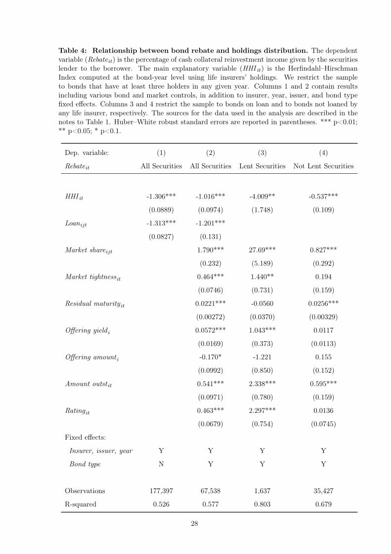
Table 4: Relationship between bond rebate and holdings distribution. The dependentvariable (Rebateit) is the percentage of cash collateral reinvestment income given by the securitieslender to the borrower. The main explanatory variable (HHI it) is the Herfindahl–HirschmanIndex computed at the bond-year level using life insurers’ holdings. We restrict the sampleto bonds that have at least three holders in any given year. Columns 1 and 2 contain resultsincluding various bond and market controls, in addition to insurer, year, issuer, and bond typefixed effects. Columns 3 and 4 restrict the sample to bonds on loan and to bonds not loaned byany life insurer, respectively. The sources for the data used in the analysis are described in thenotes to Table 1. Huber–White robust standard errors are reported in parentheses. *** p<0.01;** p<0.05; * p<0.1.
Dep. variable: (1) (2) (3) (4)
Rebateit All Securities All Securities Lent Securities Not Lent Securities
HHI it -1.306*** -1.016*** -4.009** -0.537***
(0.0889) (0.0974) (1.748) (0.109)
Loanijt -1.313*** -1.201***
(0.0827) (0.131)
Market shareijt 1.790*** 27.69*** 0.827***
(0.232) (5.189) (0.292)
Market tightness it 0.464*** 1.440** 0.194
(0.0746) (0.731) (0.159)
Residual maturity it 0.0221*** -0.0560 0.0256***
(0.00272) (0.0370) (0.00329)
Offering yield i 0.0572*** 1.043*** 0.0117
(0.0169) (0.373) (0.0113)
Offering amount i -0.170* -1.221 0.155
(0.0992) (0.850) (0.152)
Amount outst it 0.541*** 2.338*** 0.595***
(0.0971) (0.780) (0.159)
Rating it 0.463*** 2.297*** 0.0136
(0.0679) (0.754) (0.0745)
Fixed effects:
Insurer, issuer, year Y Y Y Y
Bond type N Y Y Y
Observations 177,397 67,538 1,637 35,427
R-squared 0.526 0.577 0.803 0.679
28

Table 5: Relationship between fraction lent and weighted average market sharein the portfolio. We divide life insurers’ portfolios into groups according to rebate quantile.The dependent variable Loanqjt is the fraction of bonds in group q lent by insurer j at timet. The main explanatory variable (Market shareqjt) is the fair-value-weighted average holdingof bonds in group q by insurer j relative to the total amount of the bonds made available tosecurities borrowers by all lenders. Columns 1 and 4 divide the porfolios into 32 and 64 groups,respectively, and include controls for various bond and market characteristics as well as insurerand year fixed effects. Columns 2 and 3 and Columns 5 and 6 divide the groups into those thatare above and below the median, respectively. The sources for the data used in the analysisare described in the notes to Table 1. Huber–White robust standard errors are reported inparentheses. *** p<0.01; ** p<0.05; * p<0.1.
Dep. variable: (1) (2) (3) (4) (5) (6)
Loanqjt All 32 parts 32 parts All 64 parts 64 parts
perc. > 50 perc. ≥ 50 perc. perc. > 50 perc. ≥ 50 perc.
Market shareqjt 7.806** 9.984** 9.081* 5.242** 9.684** 4.736
(3.532) (5.028) (5.013) (2.463) (3.801) (3.301)
Rebateqt -27.13*** -41.13*** -28.23*** -28.10*** -55.50*** -30.28***
(3.060) (15.46) (3.439) (2.677) (11.24) (2.926)
HHI qt -5.496*** -5.614*** -4.974*** -3.910*** -3.150** -3.709***
(1.202) (1.851) (1.602) (0.813) (1.367) (0.978)
Residual matqt -0.0562 0.0179 -0.110* -0.0139 0.0807* -0.0934**
(0.0432) (0.0612) (0.0606) (0.0312) (0.0464) (0.0410)
Offering yieldqt -0.217* -0.00620 -0.386** -0.282*** -0.158 -0.368***
(0.123) (0.185) (0.164) (0.0836) (0.150) (0.101)
Offering amtqt 0.471*** 0.335*** 1.630*** 0.473*** 0.384*** 1.457***
(0.115) (0.117) (0.339) (0.0992) (0.0974) (0.302)
Amt outstqt 0.110 0.234* -0.720 0.179 0.274** -0.252
(0.141) (0.136) (0.500) (0.132) (0.134) (0.405)
Ratingqt 0.0385 0.0260 0.0444 0.0216 0.0119 0.0113
(0.0652) (0.0968) (0.0913) (0.0510) (0.0730) (0.0705)
Fixed effects:
Insurer, year Y Y Y Y Y Y
Observations 9,941 4,926 5,015 16,703 8,208 8,495
R-squared 0.340 0.373 0.359 0.287 0.314 0.304
29
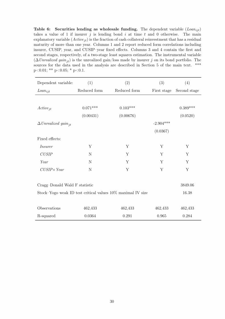
Table 6: Securities lending as wholesale funding. The dependent variable (Loanijt)takes a value of 1 if insurer j is lending bond i at time t and 0 otherwise. The mainexplanatory variable (Activejt) is the fraction of cash collateral reinvestment that has a residualmaturity of more than one year. Columns 1 and 2 report reduced form correlations includinginsurer, CUSIP, year, and CUSIP–year fixed effects. Columns 3 and 4 contain the first andsecond stages, respectively, of a two-stage least squares estimation. The instrumental variable(∆Unrealized gainjt) is the unrealized gain/loss made by insurer j on its bond portfolio. Thesources for the data used in the analysis are described in Section 5 of the main text. ***p<0.01; ** p<0.05; * p<0.1.
Dependent variable: (1) (2) (3) (4)
Loanijt Reduced form Reduced form First stage Second stage
Activejt 0.071*** 0.103*** 0.389***
(0.00431) (0.00676) (0.0520)
∆Unrealized gainjt -2.904***
(0.0367)
Fixed effects:
Insurer Y Y Y Y
CUSIP N Y Y Y
Year N Y Y Y
CUSIP×Year N Y Y Y
Cragg–Donald Wald F statistic 3849.06
Stock–Yogo weak ID test critical values 10% maximal IV size 16.38
Observations 462,433 462,433 462,433 462,433
R-squared 0.0364 0.291 0.965 0.284
30
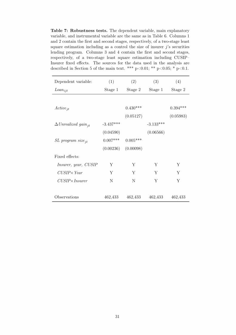
Table 7: Robustness tests. The dependent variable, main explanatoryvariable, and instrumental variable are the same as in Table 6. Columns 1and 2 contain the first and second stages, respectively, of a two-stage leastsquare estimation including as a control the size of insurer j’s securitieslending program. Columns 3 and 4 contain the first and second stages,respectively, of a two-stage least square estimation including CUSIP–Insurer fixed effects. The sources for the data used in the analysis aredescribed in Section 5 of the main text. *** p<0.01; ** p<0.05; * p<0.1.
Dependent variable: (1) (2) (3) (4)
Loanijt Stage 1 Stage 2 Stage 1 Stage 2
Activejt 0.430*** 0.394***
(0.05127) (0.05983)
∆Unrealized gainjt -3.437*** -3.133***
(0.04590) (0.06566)
SL program sizejt 0.007*** 0.005***
(0.00236) (0.00098)
Fixed effects:
Insurer, year, CUSIP Y Y Y Y
CUSIP×Year Y Y Y Y
CUSIP×Insurer N N Y Y
Observations 462,433 462,433 462,433 462,433
31
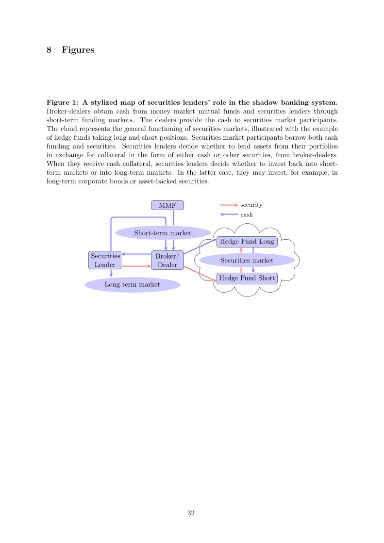
8 Figures
Figure 1: A stylized map of securities lenders’ role in the shadow banking system.Broker-dealers obtain cash from money market mutual funds and securities lenders throughshort-term funding markets. The dealers provide the cash to securities market participants.The cloud represents the general functioning of securities markets, illustrated with the exampleof hedge funds taking long and short positions. Securities market participants borrow both cashfunding and securities. Securities lenders decide whether to lend assets from their portfoliosin exchange for collateral in the form of either cash or other securities, from broker-dealers.When they receive cash collateral, securities lenders decide whether to invest back into short-term markets or into long-term markets. In the latter case, they may invest, for example, inlong-term corporate bonds or asset-backed securities.
Broker/Dealer
MMF
Short-term market
Securities market
Hedge Fund Long
Hedge Fund Short
SecuritiesLender
Long-term market
cashsecurity
32
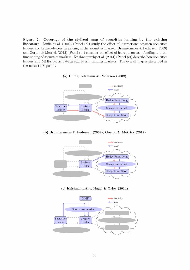
Figure 2: Coverage of the stylized map of securities lending by the existingliterature. Duffie et al. (2002) (Panel (a)) study the effect of interactions between securitieslenders and broker-dealers on pricing in the securities market. Brunnermeier & Pedersen (2009)and Gorton & Metrick (2012) (Panel (b)) consider the effect of haircuts on cash funding and thefunctioning of securities markets. Krishnamurthy et al. (2014) (Panel (c)) describe how securitieslenders and MMFs participate in short-term funding markets. The overall map is described inthe notes to Figure 1.
(a) Duffie, Gârleanu & Pedersen (2002)
Broker/Dealer
MMF
Short-term market
Securities market
Hedge Fund Long
Hedge Fund Short
SecuritiesLender
Long-term market
cashsecurity
(b) Brunnermeier & Pedersen (2009), Gorton & Metrick (2012)
Broker/Dealer
MMF
Short-term market
Securities market
Hedge Fund Long
Hedge Fund Short
SecuritiesLender
Long-term market
cashsecurity
(c) Krishnamurthy, Nagel & Orlov (2014)
Broker/Dealer
MMF
Short-term market
Securities market
Hedge Fund Long
Hedge Fund Short
SecuritiesLender
Long-term market
cashsecurity
33
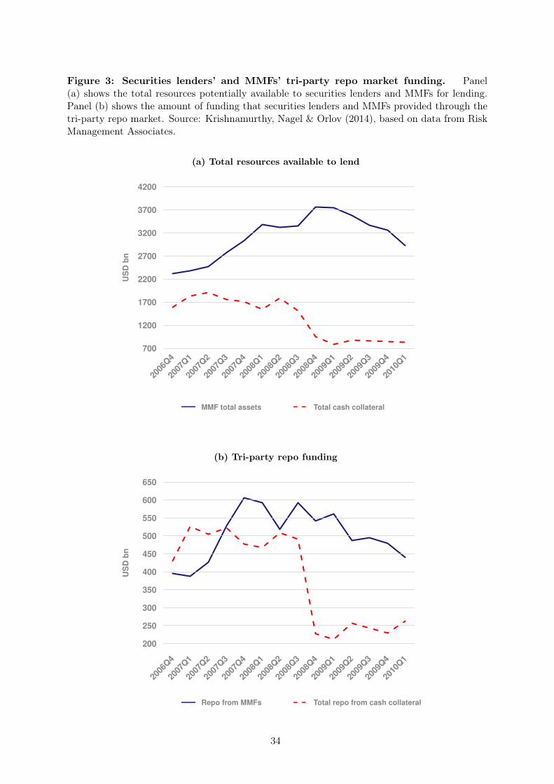
Figure 3: Securities lenders’ and MMFs’ tri-party repo market funding. Panel(a) shows the total resources potentially available to securities lenders and MMFs for lending.Panel (b) shows the amount of funding that securities lenders and MMFs provided through thetri-party repo market. Source: Krishnamurthy, Nagel & Orlov (2014), based on data from RiskManagement Associates.
(a) Total resources available to lend
700
1200
1700
2200
2700
3200
3700
4200
US
D b
n
2006
Q4
2007
Q1
2007
Q2
2007
Q3
2007
Q4
2008
Q1
2008
Q2
2008
Q3
2008
Q4
2009
Q1
2009
Q2
2009
Q3
2009
Q4
2010
Q1
MMF total assets Total cash collateral
(b) Tri-party repo funding
200
250
300
350
400
450
500
550
600
650
US
D b
n
2006
Q4
2007
Q1
2007
Q2
2007
Q3
2007
Q4
2008
Q1
2008
Q2
2008
Q3
2008
Q4
2009
Q1
2009
Q2
2009
Q3
2009
Q4
2010
Q1
Repo from MMFs Total repo from cash collateral
34

Figure 4: Securities lending against cash collateral in the United States. Thesedaily data aggregate the fair value of all securities lent against cash collateral in the UnitedStates, including equity, Treasuries, agency securities, and corporate bonds. The category ofother lenders includes corporations, endowments, foundations, and government bodies. Source:authors’ calculations based on data from Markit Securities Finance.
0.3
.6.9
1.2
1.5
Trilli
ons o
f U
S$
0.3
.6.9
1.2
1.5
Trilli
ons o
f U
S$
2007 2008 2009 2010 2011 2012 2013 2014 2015
Retirement & Pension Plans Mutual Funds
Insurance Other
35
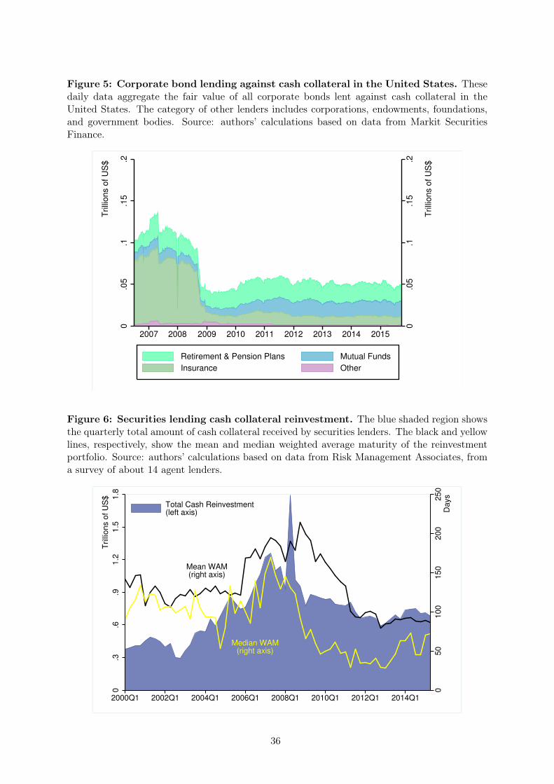
Figure 5: Corporate bond lending against cash collateral in the United States. Thesedaily data aggregate the fair value of all corporate bonds lent against cash collateral in theUnited States. The category of other lenders includes corporations, endowments, foundations,and government bodies. Source: authors’ calculations based on data from Markit SecuritiesFinance.
0.0
5.1
.15
.2
Trilli
ons o
f U
S$
0.0
5.1
.15
.2
Trilli
ons o
f U
S$
2007 2008 2009 2010 2011 2012 2013 2014 2015
Retirement & Pension Plans Mutual Funds
Insurance Other
Figure 6: Securities lending cash collateral reinvestment. The blue shaded region showsthe quarterly total amount of cash collateral received by securities lenders. The black and yellowlines, respectively, show the mean and median weighted average maturity of the reinvestmentportfolio. Source: authors’ calculations based on data from Risk Management Associates, froma survey of about 14 agent lenders.
Mean WAM(right axis)
Median WAM(right axis)
050
100
150
200
250
Days
0.3
.6.9
1.2
1.5
1.8
Trilli
ons o
f U
S$
2000Q1 2002Q1 2004Q1 2006Q1 2008Q1 2010Q1 2012Q1 2014Q1
Total Cash Reinvestment(left axis)
36

Figure 7: Securities lending by U.S. life insurers. The line shows the quarterly amount ofcash collateral received by U.S. life insurers through their securities lending programs. Source:authors’ calculations based on data from NAIC Quarterly Statutory Filings.
40
45
50
55
US
D b
n
2011q1 2011q3 2012q1 2012q3 2013q1 2013q3
Figure 8: Maturity mismatch in the securities lending programs of U.S. life insurers.Each box-and-whisker plot represents the distribution of U.S. life insurance companies, with thesolid area covering the 25-th to 75-th percentiles and the line within the solid area showing themedian of the distribution. The whiskers reflect the remaining observations, up to 1.5 times theinterquartile range, and the dots are outliers. The blue plot is calculated using the weightedaverage maturity of the cash collateral that life insurers received for lending securities, wherethe weights are the amounts of cash collateral received. The red plot is calculated using theweighted average maturity of life insurers’ reinvestment portfolio, where the weights are theamounts reinvested. Source: authors’ calculations based on data from NAIC Annual StatutoryFilings.
0200
400
600
800
1,0
00
Days
2011 2012 2013
WAM of cash collateral received
WAM of reinvestment portfolio
37