Self-Mass and Equivalence in

Special Relativity

By J. KALCKAR, J. I.I ND HARD and O. ULFBECK

Det Kongelige Danske Videnskabernes SelskabMatematisk-fysiske Meddelelser 40 : 1 I

Kommissionær: Munksgaard

København 1982

2

40:11

ContentsPage

§1. Introduction 3Basic equivalence. The classical electron model.

§2. Self-Mass and Self-Force of Accelerated Systems 7Mass determined from forces and acceleration. Electrostatic self-mass. Basic equationsmotion. Shortcomings of standard formulae. Self-mass for point force.

§3. Systematic Description by Means of Accelerated Reference Frame 15Basic properties of Møller box. Electrostatic interactions in the Møller box. Equivalencefor kinetic energy.

§4. Equivalence for Atomic Binding Energies 21Classical hydrogen atom. Quantal hydrogen atom. The Dirac equation. Thomas-Fermiatom.

§ 5. Conclusions and General Outlook 29

Appendix A. Electrodynamics in Møller Box 33

Appendix B. Static Potentials in Møller Box 36

Appendix C. Klein-Gordon Equation in Møller Box 39

References 42

SynopsisWe study dynamical aspects of equivalence between mass and energy, for systems of interactingparticles. The starting-point consists in the classical formulae for electromagnetic self-momentum,self-energy and self-force. These formulae possess puzzling terms which have been subject to variousexplanations, like compensating Poincare stresses, or were bypassed through attempts of redefini-tion of the classical electron model. By means of a comprehensive study of acceleration processes weshow that there is a crucial error in the usual derivations of self-force. We derive a basic accelerationequation for a point-like system, with detailed equivalence. It also follows that the standard formulaefor self-energy and self-momentum are, at best, misleading. Next, we study how systems are to bedescribed in an accelerated, rigid coordinate frame — the Møller box. In considerable detail weinvestigate classical and quantal equations of motion for fields and for particles in the Møller box,including the Dirac equation for the hydrogen atom, arriving at equivalence. Finally we discussproperties of composite systems as compared with properties of particles.

JØRGEN KALCKAR, OLE ULFBECK

JENS LINDHARDNiels Bohr Institute Institute of PhysicsUniversi ty of Copenhagen University of Aarhus

Denmark

© Det Kongelige Danske Videnskabernes Selskab 1982Printed in Denmark by Bianco Lunos Bogtrykkeri A/S, ISSN 0023-3323. ISBN 87-7304-124-6

40:11 3

§1. IntroductionThe present paper contains a study of equivalence between mass and energy, fora system of interacting particles. This question may appear trivial from the pointof view of general principles in special relativity, for there can be no doubt aboutthe validity of equivalence as a basic statement. But if we turn to actual calcula-tions on systems with Coulomb interaction, we find that the resulting self-energies and self-momenta do not correspond to equivalence, and lack four-vectorproperties. This is certainly surprising to the uninitiated, for one would expectbeforehand that the Maxwell equations must give equivalence unambiguouslyand in a straightforward manner, since special relativity, in a sense, is suspendedin the Maxwell equations. It should be added that the results in question haveoften been treated in connection with the problem of electron self-energieswhere they apparently required the presence of non-electromagnetic forces.Because of the complications, some authors have preferred to define an electro-magnetic energy-momentum four-vector for the electron'''. This will hardly do,however. The basic classical case is not an electron, but a macroscopic system,for which one is not free to define the electromagnetic self-energy or self-momentum.

These preliminary comments will be enlarged upon in the remainder of thischapter. But they indicate the aim of the present paper. In fact, we hope toconvince the reader that simple acceleration processes, if studied with care,reveal that there is not only equivalence, but even detailed equivalence: eachindividual term of, e.g., the interaction energy, has separate equivalence. Thebasic conclusions in this respect are contained in §2, where the connection between

mass, forces and acceleration is studied. A central issue is the question of com-parison of forces acting in different points of a system. In § 3 is presented the moresystematic treatment of accelerated frames of reference. Next, in § 4, we calculatethe various contributions to self-mass in a number of classical and quantal cases,including the Dirac equation for a hydrogen atom.

As outlined, our study has an immediate background. But it is also a necessarystep in a more general pursuit: the endeavour to understand composite systems

4 40:11

and elementary particles, including the connection between them and betweentheir classical and quantal descriptions. At the end of this paper, in § 5, we outlinegeneral viewpoints on this matter.

Basic equivalence

The equivalence between energy and inertial mass was first established by Ein-stein' (cf. also v. Laue3 ). He considered the change suffered by a system emittingelectromagnetic radiation. The usual derivation consists in showing, first, that

the energy E and momentum P of any closed system constitute a four-vector.The basis for this result is the special principle of relativity, combined with con-servation of energy and momentum for initial and final states of a collision process(corresponding to Einstein's idealized experiments). Second, the four-vectormay be written as

E = E'y,

P E= yv,

where E' is a constant, and

= 1

Y (1 _ V2/e2)1/2 •

Now, on the one hand, E' in (1.1) has to be the energy of the system in the restframe. On the other hand, E'/c 2 in (1.2) must be the mass M of the system,belonging to the non-relativistic limit v < c, and so we obtain equivalence,

M = 2.c (1.3)

Equivalence is therefore derived by comparing initial and final states of anelastic or inelastic process. The proof concerns not only a stable system ; it includesunstable systems. Although it appears that the proof of equivalence is concernedwith only the total energy of a system, still there are evidently cases where partof the energy must have equivalence. Moreover, one can divide the total energyof a system into well-defined average contributions from various forms of energy,as exemplified by the virial theorem. Beforehand, one would expect individualequivalence from these clearly separated contributions. Thus, it is natural toinvestigate the possible validity of detailed equivalence, as formulated in thepreamble.

The previous results may be put on a more comprehensive form if we introducethe Lagrangian of the system. In fact, the above momentum-energy four-vector

(1.2)

40:11 5

with its derivation from collisions, must be connected to a variational principle,albeit with limited validity. In an inertial frame where the system has velocity y,the corresponding Lagrangian must be

v22)112.L=—E' 1— c

In this formula the internal energy E' is a constant of the motion for a giveninternal state of the system. If we now observe the given system from anotherframe, where it has velocity v+ 8v, the change 8L becomes

(SE = 8v-P, (1.5)

where Pis given by (1.2). Furthermore, the quantity E = —L + v •P correspondsto (1.1).

In (1.5) we are concerned with a variation where the internal state of thesystem is kept unchanged. Thus, we have obtained equivalence, E' = Me e , bybeing able to separate the external velocity variable, y in (1.4), from the internalvariables of the system, concealed in the constant E'. Moreover, for soft collisions

if the internal state of the system is not changed during a collision — the equa-tion of motion will be based on (1.4), i.e. the kinetic contribution to the totalLagrangian.

In itself, eq. (1.4) reasserts the surmises about detailed equivalence madeabove. Thus, when the system is in internal statistical equilibrium, and E'separates into definite terms according to the virial theorem, these terms shouldcontribute separate mass terms in the account of the system.

The classical electron model

Already before the advent of special relativity, Poynting's theorem of density offield energy was utilized in several calculations of self-energy and self-momentumof a charged body (cf. e.g. Jammer 4 ). The foremost contribution was made byLorentz'. The results were hardly changed at all by special relativity. We shallillustrate the situation in terms of the so-called classical electron model, as quotedin numerous monographs (e.g., Jackson', Pais', Feynman7).

Consider then a stable spherical shell with radius a, on which a total chargeQis uniformly distributed. In a inertial frame K the shell moves with velocity v.According to standard results, the densities of momentum and energy of anelectromagnetic field are given by the field strengths

g(r,t) = 4 ^ cE(r,t) X B(r,t) ,

(1.4)

(1.6)

6 40:11

u(r,t) = 8n(E2(r,t)+B2(r,t)).

In these equations we introduce the field belonging to the shell, as observedin the frame K. By integrating over all space we find a momentum Pet and anenergy

E, (cf. Jackson', Becker and Sautere, Rohrlich9)

2Pe, = d3rg(r,t)= 3 Yv , (1.8)

Eel =f (13 r u(r,t) =Qa Y(1+3 Cz^ (1.9)

In particular, it is seen that, in the rest frame, the momentum is P^, = 0, and theenergy Ee', = Q2 /2a. Therefore it follows that not only is equivalence lacking,

but also Pe„ Ee„ Pe„ and Eel fail to transform like the four-vector (1.1), (1.2).As is well known, this curious result cannot be rejected out of hand, the reasonbeing that Pe, and E e, do no represent the total momentum and energy of theshell. The shell in question must in any case be stabilized by other, nonelectro-magnetic, forces. These forces, or Poincaré stresses, should then compensate theerratic behaviour of (1.8), (1.9), giving a correct total four-vector.

The results (1.8) and 1.9) are obtained somewhat indirectly, in a sense. Theirbasis, i.e. the densities (1.6) and (1.7), was derived in turn by studying the actionof forces from material charges on an electromagnetic field. Therefore, by omittingthe intermediate step (1.6), there should be a more direct, but apparentlyequivalent, way of obtaining the self-mass due to Coulomb interaction. In fact,one can instead find the electromagnetic self-force of an accelerated shell ofcharge. An early calculation of this kind was performed by Born 10 (cf. alsoHeisler", and Jackson'). If the shell is momentarily at rest, but accelerated, attime t = 0, one may find the electric field E s (r,t) caused by it. We assume thatthe acceleration is small, or ga/c 2 << 1. It follows that Es (r,t) is linear in g. Letfurther Q(r) denote the internal charge distribution of the shell. The total self-

force Fs is then linear in the acceleration

Fs = fd3 rQ (r)Es (r,t = 0) . (1.10)

By these means the self-mass was calculated as the ratio F s /g, the result being inagreement with (1.8).

It thus looks as if the previous result (1.6) has been vindicated in an elemen-tary way by the self-force (1.10). The latter becomes our starting-point, however.For although it concerns non-relativistic motions and an apparently innocent

acceleration process, still this process contains unexpected relativistic pitfalls,and (1.10) is not connected to the self-mass, as we shall see ind §2.

(1.7)

40:11 7

§2. Self-Mass and Self-Force of Accelerated Systems

In this chapter we attempt to find the way in which inertial mass can be deter-mined by means of acceleration processes. Since we know that there may behidden difficulties in this problem, we try to be careful — and thereby perhapsoverly cautious — in deriving the relativistic connection between acceleration,forces, and mass. We do it in two steps. First, we look for the physically simplestacceleration process for a system of finite size. Next, we find the expression forthe mass of a system, given in terms of its acceleration and the forces acting on it.We will then be ready to find actual self-masses for charged systems, and havealso prepared the way for the more systematic treatment in the following chapters.

The problem at hand can be exemplified by an elastic body originally at rest,and in equilibrium, in an inertial frame. We want to transfer it to anotherinertial frame, where it should finally be at rest and in the same state of equilibriumas before. The simplest way in which to bring about this change is to have anadapted acceleration of the various parts of the system, such that it is moved asif it were rigid. In fact, by means of the idealized process of rigid acceleration weavoid producing internal stress or excitations in the system, as well as growingdeformations. It would of course be possible to employ acceleration processesother than the rigid one; they would be more complicated, however, and wouldneed the rigid acceleration as a standard of reference.

Rigid acceleration

As our first step we therefore consider the kinematical consequences of rigidacceleration of a static system. Then there exist successive frames in which thevelocities of all constituent particles vanish simultaneously. Consequently the

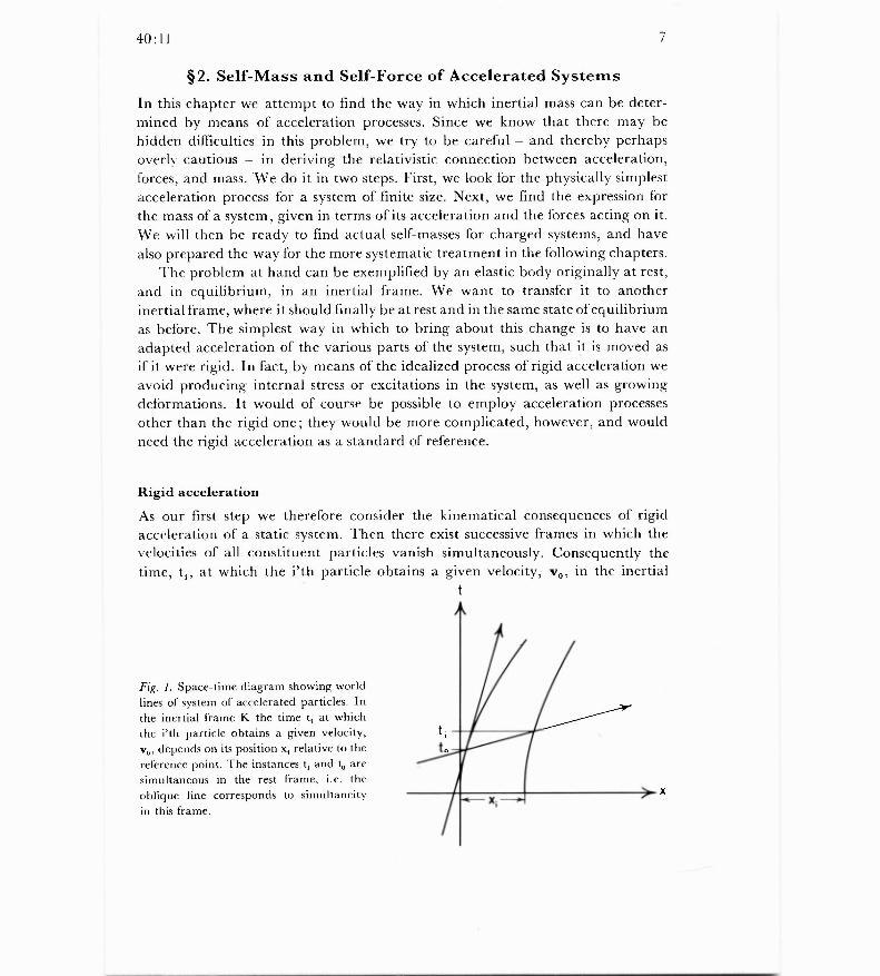
time, t ; , at which the i'th particle obtains a given velocity, v o , in the inertial

Fig. 1. Space-time diagram showing worldlines of system of accelerated particles. Inthe inertial frame K the time t ; at whichthe i'th particle obtains a given velocity,vo , depends on its position x, relative to thereference point. The instances t, and t9 aresimultaneous in the rest frame, i.e. theoblique line corresponds to simultaneityin this frame.

x

8 40:11

frame K depends on its position, r 1 (see Fig. 1). For constant acceleration, g ; , oft he i'the particle we then have, since we consider small time intervals and velocities,

Vo = g , t ; . (2.1)

Let us measure positions relative to some reference point chosen arbitrarily withinthe system, and let to denote the time during which the reference point has beenaccelerated with acceleration g„ . Since the instances t o and t ; in the frame Kmust correspond to simultaneity in the rest frame, they are to first order in vacrelated by the equation

tj = to+ V gr' = gCZr`).C

It therefore follows that the accelerations of the various points r; must obey therelation

go g + go 'r1/0

Thus, the acceleration of the points r; decreases in the direction of g o . This effectexactly corresponds to the Lorentz contraction of the system as measured fromthe frame K.

Mass determined from forces and acceleration

As a second step, let us study the connection between force, acceleration, andmass. The fundamental relation between the three is obtained in the idealizedcase of a point particle. In fact, consider a point particle at rest, and with mass m.If it acquires a small acceleration g, the applied force must be F = gin. More-over, during a time 8t, its change of momentum and velocity are, respectively,(Sp = F8t and åv = gat. This result has an immediate consequence. For supposethat, by applying the above force F in one point of a composite system, we obtainthe acceleration g of this point, while the system remains, internally, in a stationarystate. Since the momentum transfer and velocity change remain as before, thecomposite system must have the same mass m as the above particle. Presumably,part of its mass is then due to deformation energy caused by the acceleration.These seemingly trivial conclusions give one important clue to self-mass problems,as shown in an example at the end of this chapter.

Having verified the basic results belonging to a point force, we next consideracceleration of a system where forces are applied in several points. It followsfrom, e.g., eq. (2.3) that in special relativity there must be a somewhat intricate

connection between forces on a system, its acceleration, and its total mass. Becauseof this, and because of the important consequences, we treat the problem at handin an elementary and somewhat elaborate manner. We also want to show that

(2.2)

(2.3)

40:11 9

one is not concerned with new definitions, but instead with an inherent physical

property of accelerated systems: although the velocities are non-relativistic, wesometimes have to introduce a relativistic correction to the usual conception of

forces.Consider then a set of point masses m ; , at r., initially at rest and with no

mutual forces. By means of suitable external forces we can accelerate the massestogether, according to (2.3). We must act on them with the individual forces F;,

located at r; ,

m;Ft go 1+go•r,/c2

where the acceleration at r = 0 is g o . Now, if we compute the total force F, we

obtain

m;F = E F, = E go 1+go•rllc2

which quantity is not proportional to the total rest mass, M =the exact expression for the mass M is, by (2.4),

go M =EF;(I+g /csrt

(2.5)

. Instead,

(2.6)

In point of fact, we have here normalized all forces to the point r = 0, withacceleration go . At first, eq. (2.6) might appear to be an unnecessary elaboration,for if go is imagined to be sufficiently small, it looks as if the factors (1 +g o •r /c2)can be replaced by unity. That will also be true in many cases, but for self-forcesit is in error, because they contain large leading interaction terms, which wouldcancel if this replacement were made.

The conception of rigid acceleration may appear a little artificial for non-interacting point masses. But the idea is, as before, that we can replace this systemby an actual system of interacting masses, e.g., an elastic body. In order not todeform the body more and more during the acceleration, we must keep to theprescribed rigid acceleration. As before, the total mass of the elastic body mustbe the same as that of the non-interacting point masses, if the accelerations andforces are the same. The formula (2.6) is therefore the general expression for the

mass of the system, calculated in the simplest consistent situation.

Electromagnetic self-mass

Suppose that a system consists of charged particles, with individual masses m ; .At time t = 0 in the frame K the particles arc all at rest with separations r ;k andelectrostatic energy

(2.4)

10 40:11

i *k

U = 2 E gig k (2.7)r ', k

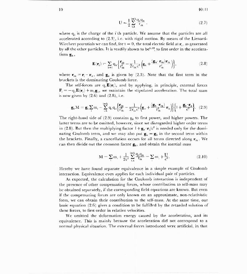
where q i is the charge of the i'th particle. We assume that the particles are allaccelerated according to (2.3), i.e. with rigid motion. By means of the Lienard-Wiechert potentials we can find, for t = 0, the total electric field at r, , as generatedby all the other particles. It is readily shown to be'' 12 to first order in the accelera-tions g k ,

E(ri) = E g k j råk— 1z (g k—^(gk' rsk)rik)}

k #i r ik 2rik e l2ik

where rik = r1 — rk , and gk is given by (2.3). Note that the first term in thebrackets is the dominating Coulomb force.

The self-forces are g i E(ri ), and by applying, in principle, external forcesF =—g 1 E(ri )+m,gi , we maintain the stipulated acceleration. The total massis now given by (2.6) and (2.8), i.e.

i$k_ c7^ f1 f1 rik 1 (gk rik)goM — go^ilni —LJ 7 i `l k{ rik 2rik cz (gk+ rik k){

{I+gOcrk}. (2.9)

The right-hand side of (2.9) contains go to first power, and higher powers. Thelatter terms are to be omitted, however, since we disregarded higher order termsin (2.8). But then the multiplying factor 1+ g„ •r ßc2 is needed only for the domi-nating Coulomb term, and we may also put gk = go in the second term withinthe brackets. Finally, a cancellation occurs for all terms directed along rik . Wecan then divide out the common factor go , and obtain the inertial mass

i * k

M = ^Ini+ 1 2 E grgk =E m i +U.2c , ,k ik

Hereby we have found separate equivalence in a simple example of Coulombinteraction. Equivalence even applies for each individual pair of particles.

As expected, the calculation for the Coulomb interaction is independent ofthe presence of other compensating forces, whose contribution to self-mass maybe obtained separately, if the corresponding field equations are known. But evenif the compensating forces are only known on an approximate, non-relativisticform, we can obtain their contribution to the self-mass. At the same time, ourbasic equation (2.6) gives a condition to be fulfilled by the retarded solution ofthese forces, to first order in relative velocities.

We omitted the deformation energy caused by the acceleration, and itsequivalence. This is mainly because the acceleration did not correspond to anormal physical situation. The external forces introduced were artificial, in that

(2.8)

(2.10)

40:11 lI

they exactly took care of maintaining the configuration of the particles withint he undisturbed system. In actual acceleration processes one can instead be con-cerned with an external electric field which is constant in space and time. Then,the configuration of the particles will be changed slightly from that of the undis-turbed system. Hereby, deformation energy, and its equivalence, can be obtained.In many cases, such deformation terms are of higher order in g o , and thereforedo not affect the basic result (2.10). We shall presently discuss a simple examplewhere deformation energy plays a major role.

Basic equation of motion

From the previous results it is easy to formulate the basic equation of motion ofcharged system momentarily at rest, and placed in a weak external electric field

Eext (r,t) varying slowly in space and time. By a slow variation in space we meanthat the relative change of Eext(r,t) is small within the system. We suppose thatthe field varies sufficiently slowly so that the system remains in a quasistationarystate. Eq. (2.9) provides an expression for the acceleration go of a standard point

ro , times the total mass M as arising from Coulomb interaction and from otherenergy contributions in the system. Next, according to (2.6) the product g o M isequal to the weighted sum of external forces,

M-E F(1+go'(c,— ro )) — ^ E (r

t) ( l + go (C, —ro )). (2.11)g0 2 / `li ext i^

Here, we expand in powers of r; —ro , and include only first order terms ont he right hand side. But since the standard point ro may be freely chosen, we place

it at the charge centre, ro = re F, q ; rt /q, where q = E q ; is the total charge of

the system. For it then turns out that first order terms in r ; —ro disappear, andwe are left with gEext (re ,t) on the right hand side of (2.11). The equation ofmotion is now simply, in the momentary rest frame,

ge M = g Eext (re , t ) )

where re is the charge centre, and ge its acceleration. Moreover, q is the totalcharge, and M the total mass of the system. Thus, the result (2.12) represents aprecise basic equation of motion of a charged system. It gives an essential modifi-

cation of the so-called Abraham-Lorentz equation; the standard factor 4/3 mul-tiplying the electromagnetic mass has disappeared, because equivalence reignsin M. In addition, eq. (2.12) contains the subtlety that the system is representedby one definite point, i.e. the charge centre re . Consequently, eq. (2.12) can beused as an equation of motion for, say, a uranium nucleus in an external electric

(2.12)

12 40:11

field, or, for a classical electron model. One may immediately correct the equationby a familiar term containing radiation damping, if so desired.

Although, as mentioned, eq. (2.12) is widely applicable, let us register maincorrections to it, or assumptions contained in it. We have assumed that theexternal field varies slowly in time. The time variation of EeX1 will, first, give riseto adiabatic changes of M and, second, to non-adiabatic mass excitations. Third,we have already mentioned that a time variation of g,, leads to radiation damp-ing. Finally, it g,. quickly changes direction, the mass centre need not remainbehind the charge centre, and rotations may be induced. In order to study that,systems with spin must be included in the description, but that is outside thescope of the present paper.

Shortcomings of standard formulae

At this stage it is convenient to compare with the standard derivation of self-forceas alluded to in §1, and performed by Heitler, for instance. In that description,the self- fields are again given by (2.8), but with gk = go , which does not lead toimmediate errors. Next, the total force is calculated, corresponding to (1.8) and(2.5), and erroneously identified with the mass times the acceleration go . Thus,from (2.8) and (1.8)

'*k 1 (go r. )F=F, _ ^ tn ' g0+ 2r, k c2 (gu+ r2

rik) (2.13)

where the dominant Coulomb terms have cancelled out, in contrast to (2.9).For a spherical symmetric charge distribution, with electrostatic energy U,

the expression (2.13) leads to

F = (E m i + 3 go

In case the charge distribution is merely symmetric about the direction of go,the factor 4/3 is seen to be replaced by a number 1+ , where 0 < < 1. For ageneral distribution, however, the force F need not even point in the direction ofg,,. We have hereby clarified in some detail the shortcomings of the Galileanconcept of a total force and its association with total mass, in special relativity.

Next, let us consider the standard formulae for self-momentum and self-energyof a charged system, i.e. (1.8) and (1.9). Although they are connected to theabove-mentioned standard self-force calculation, their short-comings are of amore elusive kind. Still, in order to elucidate their basic contents, we can observethe following. If a system has internal Coulomb energy U, then the standardself-momentum corresponding to (1.8) can be Pe, = (U/c2 )v y• (1+ ), where

(2.14)

40:11 13

= 1/3 for a spherically symmetric charge distribution. Similarly, the standardself-energy becomes E e, = U • y • (1+ ev2 /c2 ), corresponding to (1.9). Therefore, ifwe form the difference v • Pe , — E e, , we invariably get a quantity independentof e, namely

2Lei = —E,,,+V • Pe, =— U 11•(1 — V2

In point of fact, we have recovered eq. (1.4), i.e. the Lagrangian belonging toequivalence. Moreover, it is apparent that, instead of making the indirect deriva-tion of (2.15) via E e , and Pe„ we could have obtained it directly by integrationof the invariant Lagrangian density in space, as belonging to the field and toits interaction with matter, or £°aeid + Y; n , •

Returning to the Lagrangian in (2.15), we have already seen, in (1.5), thatif we vary L e, with respect to v, keeping the internal state unchanged, we arriveat the momentum P = (U/c2 )y•v, leading to equivalence. In fact, this implies

detailed equivalence, the Coulomb contribution being only part of the totalinternal energy.

Next, it also becomes clear how the standard momentum Pe , can be connectedto (2.15) : when v is varied, there is assumed to be an associated variation of theinternal state — i.e. of U. Thus, P e, will result if we let U vary proportionally to(1—v2 /0Y", when L e, is varied with respect to v. The factor in question mustbe due to a Lorentz transformation of the internal variables of the system.

We have thus realized that the standard momentum and energy (1.8) and(1.9), arise from an unwarranted variational procedure, whereby they lose con-nection to our basic concepts of momentum and energy of an isolated system, asdescribed in §1. Such results arise in general from arbitrary transformations ofinternal variables of a system, where momenta become abstract quantities, with-out direct physical significance.

Self-mass for point force

"Ihe present discussion of the central ingredients in equivalence calculations isperhaps best concluded by means of an example serving a triple purpose. First,it concerns an external point force, implying the simplest possible connection tomass and acceleration. Second, the equivalence in question applies to deforma-tion energies, not studied explicitly above. Third, Poincaré stresses cannot beintroduced.

Let two mutually repelling charges, q a and q b , be accelerated from rest alongtheir line of connection, rba . An external force Fa acts on particle a, while particleb in turn is made to accelerate by the Coulomb repulsion from particle a. The

(2.15)

14 40:11

force and distance rab are balanced such that the particles are accelerated inrigid motion. The internal energy of the system, cl a ck/raj) , is purely an energy ofdeformation. The internal electric fields are given by (2.8), and so the equationsof motion of the two particles become

g a q b gaqbma g es = rab rab — rab e2gt• + Fa ,

g a q b _ gaqbmbgb = 3 rba 2 g;i

rab rab e

where all vectors are collinear, while m a and m b are mechanical masses. Further,the condition of rigid acceleration determines gb in terms of ges and rba , cf. (2.3),

_ ges(2.18)gb 1 +ges •rba/c2

We multiply (2.17) by l + (ges •rba )/c2 , add (2.16), and obtain to first orderin ges

F= ga (m a + Mb+ grq b 1 2 1. (2.19)

ab C )

Since the mass M of the system must be given by Mga = Fa , we find

M = ma +mb + grgb c2 •

In the simplest imaginable case we have thus obtained equivalence, and for adeformation energy in fact.

Let us next turn to the standard procedure, where the total self-force iscalculated, cf. (2.13) or (1.10). It corresponds to adding the right-hand sides of(2.16) and (2.17), omitting F es . The self-mass becomes erroneous, or 2gagb/(rabc2),like in (2.13). We might similarly, as done by Heitler, add (2.16) and (2.17) withthe Galilean demand gb = g es , and obtain a wrong value of the force Fa . In anycase, there are here no compensating Poincaré stresses, which can repair the error.

Whereas, in the present chapter, we have arrived at the proper treatmentbelonging to coordinates (inertial frames) where equations of motion are simplebut self-mass calculations delicate, the theme in the following will be reversed.In fact, we shall introduce coordinates (Møller box) where self-mass calculationsbecome extremely simple; our task will be to obtain the equations of motion.Thereby, the discussion becomes lengthy, containing transformations of equa-tions of motion in various classical and quantal cases.

(2.16)

(2.17)

(2.20)

40:11 15

§ 3. Systematic Description by Means ofAccelerated Reference Frame

Basic properties of Møller box

The previous chapter contained a preliminary analysis of simple accelerationprocesses for which the intrinsic state remained stationary in the instantaneousrest frame. A systematic analysis of such processes must be based on a descriptionof the system in an accelerated rigid frame of reference, always coinciding withthe instantaneous rest frame. A coordinate system of this kind, where each pointhas a time independent acceleration in its momentary rest frame, we shall referto as a Møller box*).

Before embarking on a detailed discussion of the Møller box, we may pointout some of its salient features. First, the physical laws in the box are independentof time, i.e. there is invariance against time displacement and time-reflection.Second, there is an inborn simultaneity, like in a static gravitational field. Third,it also follows that a charge at rest in the Møller box gives rise to a purely elec-trostatic fi eld in this frame. This feature corresponds to the fact that for a staticcharge in the box, performing a hyperbolic motion in an inertial frame, the

retarded and advanced fields are identical within the box. Fourth, in the inertialframe we had to distinguish between, on the one hand, that weighted sum offorces which leads to the total mass of a system and, on the other hand, the totalforce. In the Møller box these concepts are united in the sense that the totalforce required to keep a body at rest in the box is proportional to the total massof the body.

When introducing the Møller box it is useful to consider first the hyperbolicmotion of a single particle. Let a particle in an inertial frame K be acceleratedalong the X-axis, with the constant acceleration g o in its rest frame. It is convenientto introduce the length A = c2 /go and write for the trajectory

Xo =.îcosh j, Yo =Zo =0, (3.1)

cTo = A sin h

Thus, the coordinates cTo and Xo lie on the hyperbola

Xå-c 2 Tô =.12 . (3.2)

*) Accelerated rigid frames of reference are discussed in some detail by C. Møller in his mono-graph on relativity13. We have adopted the name Møller box for the particular frame discussed inthe text. The wording box is meant to indicate that we are considering a space-time domain offinite extension.

16 40:11

Here (To , X0 , Yo , Zo ) are the particle coordinates in the inertial frame K, and tdenotes proper time for the particle. For this motion the four-velocity

Uo = ( d (d t dd o'

0,0) _ A (X0,cT0,0,0)

(3.3)

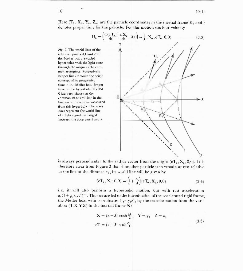
Fig. 2. The world lines of thereference points 0,1 and 2 inthe Møller box are scaledhyperbolae with the light conethrough the origin as the com-mon asymptote. Successivelysteeper lines through the origincorrespond to progressivetime in the Møller box. Propertime on the hyperbola labelled0 has been chosen as thecommon standard time in thebox, and distances are measuredfrom this hyperbola. The wavylines represent the world lineof a light signal exchangedbetween the observers 1 and 2.

2

is always perpendicular to the radius vector from the origin (eT0 , Xo , 0,0) . It istherefore clear from Figure 2 that if another particle is to remain at rest relativeto the first at the distance x 1 , its world line will be given by

(cT1 ,Xt ,0,0) = (l+)(cT0,Xo,O,0) (3.4)

i. e. it will also perform a hyperbolic motion, but with rest accelerationgo (1 +goxl/c2)-'. Thus we are led to the introduction of the accelerated rigid frame,the Møller box, with coordinates (t,x,y,z), by the transformation from the vari-ables (T,X,Y,Z) in the inertial frame K:

X= (x+,1)cosh ^ , Y=y, Z=z,

cT = (x+ .1) sinh ,(3.5)

40:11

corresponding to the line element

/

ds2 = c2 dT'2 — 2 = I 1 + 1)2 c2 dt2 — dr2 .

For T = t = 0 we have X = x +A, where we have selected a standard hyperbolafrom which we measure distances along the x-direction in the box. The propertime t of the standard hyperbola x = 0 has been chosen as the common standardtime variable in the box. Hence, outside the standard hyperbola, local propertime deviates from standard time. In fact, the relation between standard time tand local proper r at the position x is given by

dr = (l+ --)dt.

The choice of the standard time t in the Møller box makes explicit the in-variance against time displacement and time reflection inherent in this staticreference frame. Therefore, this way of synchronizing events corresponds to theinborn simultaneity in the box. This can be illustrated by considering a lightsignal moving along the x-axis between two observers 1 and 2 at rest in the box(see figure 2). We assume that the light signal is sent back at time T = 0. Wenotice that since each hyperbola corresponds to the locus of constant distancefrom O in Minkowski space, they are symmetric with respect to the radius vectorsin this space. We have therefore drawn the figure such that the inherent symmetryof the hyperbolae is made explicit with respect to the axis T = 0. Events on theline OB° B, are simultaneous with the departure of the light signal from the firstobserver, and events on the line 0A 0 A, are simultaneous with its return. It isobvious from the figure that if the events are synchronized to proper time of thestandard hyperbola x = 0, the time of arrival to the second observer will be half-way between the time of departure from the first observer and the time of return.This result is also directly borne out by evaluation of the standard time intervalsin question, which are found to be (2/c) log [(x2+ .i.)/(x,+.1)], x, and x2 beingthe coordinates of the two observers.

It follows from the transformation (3.5) that a particle at rest in the Møllerbox at position x at time T = t = 0 has acceleration

c2 go g(x) —a+x— 1+gox/c2

in the inertial frame. This is of course the result (2.3) already deduced for therigid acceleration in the inertial frame. In contrast, a particle at rest at T = t = 0in the inertial frame at the same position X = x+ .1, in the Møller box has anacceleration

17

(3.6)

(3.7)

(3.8)

18 40:11

åt2 =—g (1 +2

o - (3.9)

Thus (3.9) expresso the acceleration of a freely falling particle in the coordinatesof the Møller box. It has of course the opposite sign of (3.8), but, more important,its magnitude increases in the direction of go in contrast to g(x).

The line element (3.6) implies a simple scaling law for velocities. In particular,the velocity of light in the box is given by

c(x)=c•(I+gc%2).

In fact, whereas the velocity of light in local units is alsays c, it must be changedby the factor in (3.7) when we measure in standard time.

Electrostatic interactions in Møller Box

In this section we shall be concerned with charged particles moving in staticpotentials*). The field equations for static potentials in the Møller box arederived from the action principle

SS f +SS,nt = 0, (3.11)

where the contributions to the action from the field and the interaction areobtained from the general expressions (A13) and (A14) :

S t = — Aid t Jd3 r (1(+ x/A ) , (3.12)

S, nt =— feltid 3 re(r)v(r) . (3.13)

If (3.11) corresponds to variation of the potential ip for fixed charge distribu-tion e, one obtains to first order in A

_ 1 = go /c2 the result

Av(r) ,1 aaxr) - -4n(1 +3)e(r)•

*) For the sake of completeness, a discussion of electrodynamics and the equations of motion ofcharged particles in the Møller box is given in appendix A, while the static potentials are solved inappendix B.

(3.10)

(3.14)

40:11 19

Consider the potential (r ;r1 ) in the point r generated by the charge densityg(r) = g 1 S(r—r1 ), i.e. by a single charge q1 at rest in the point r1 . According to(3.14) this potential is to first order in 112

(r ;r1 ) -= g'(1+

x2^x1^ (3.15)

r — rl

In order to appreciate the significance of the second term in the brackets in(3.15), consider a second charge q 2 at rest at the position r2 . We notice that thedensity of the interaction energy of two charges depends on the values of the twocharges only through their product. We therefore expect that the position of thecentre-of-mass of the interaction energy is always the same as for two identicalcharges, namely midway between them. Thus, in the interaction energy q 2 tp (r2 ;r1)

we can interpret the term

91 c:2 x2 +x i SEint — I l 2 go 2

r2 — rl c

as the potential energy of a mass g192/c21r2 —re l located at the midpoint betweenthe charges in the artificial gravitational field g o . The energy (3.16) thereforerepresents the work required to lift a mass equivalent to the Coulomb energy fromthe reference level x = 0 to the height (x 1 +x2 )/2. Hence we expect that the sumof the mutual forces be equal to ( g 1 g2/ c2 I r2 —r1 ) go • This is indeed in accordancewith (3.15), from which it follows that

9z a V(r2 ; r1)g1 (ri ; r2) — 9192

goa —1.1 H2

This relation, which embodies the equivalence between electrostatic energyand mass, will be crucial in the following discussion. It corresponds to the weightedaddition of forces (2.6), applied to the Coulomb case (2.8), but in the Møllerbox it emerges as a direct consequence of the term (3.16) in the interaction energy.

The equations of motion in the Møller box, for a particle of mass m andcharge q moving in a static potential rp, is obtained from the action principle

SSkin + SSi„t = 0, (3.18)

with

S =—mc2jdr=—mc2J d t1(1+ )2—c211î2

kin

(3.16)

(3.17)

(3.19)

S 1nt = — J dtqv(r(t)) . (3.20)

20 40:11

If (3.18) corresponds to variation of the particle coordinates for fixed potential,one obtains the equations of motion of the particle. They correspond to theLagrangian

L = —mc2 {(I+1)2 — C:}1/2— q(r) •

Equivalence for kinetic energy

The first term in the Lagrangian (3.21) turns out to contain separate equivalencefor kinetic energy. In order to illustrate this property let us consider a ball ofmass m, bouncing between ceiling and floor of a small rectangular enclosurewhich is kept at rest in the Møller box, with its floor at the reference level x = 0,and with its edges parallel to the coordinate axis. Let the ball jump from thefloor with momentum p,t (1) in the x-direction and hit the ceiling after a time Twith momentum p x (2) along this direction. We assume that the enclosure is sosmall that the kinetic energy of the ball can be regarded as constant during itsmotion. Consequently the net momentum transfer per unit time from the ballto the box is

T T

p x( 2 ) —p x( 1 ) _ 1 ^ dt dpx — l Idt

al, m go T T dt T a x — (1—

v2/c2)u2'o o

where we have used the equation of motion corresponding to the first term ofthe Lagrangian (3.21). In order to keep the enclosure at rest in the Møller box,the presence of the bouncing ball thus requires an extra force 8F so as to supportthe floor of the enclosure

8i =(1—v/c2)i2go. (3.23)

This force is the same in the Møller box as in the particular inertial frame,which momentarily coincides with the enclosure, since standard time coincideswith proper time at the location x = 0.

However straightforward this demonstration of separate equivalence forkinetic energy may appear, one should note that it stands in contrast to theconventional treatment of similar examples. In fact, in the latter approachequivalence can only be stablished by explicitly taking into account the stressesset up in the walls by the bouncing ball, and would not apply to the kinetic energyseparately.

(3.21)

(3.22)

40:11 21

§4. Equivalence for Atomic Binding EnergiesSo far we have discussed quite idealized systems in which there was either electro-static or kinetic energy present. As a simple example of a more realistic physicalsystem with both kinetic and potential energy, we consider a hydrogen atom andenquire into the total force necessary to keep the nucleus at rest at the position

rn = 0 in the Møller box. This force is the same in the Møller box as in that inertial

frame in which the nucleus is momentarily at rest, since standard time coincideswith proper time at the position r = 0. For simplicity we treat the atom as a one-particle system, i.e. we neglect the motion of the heavy nucleus around the masscentre.

The atom is assumed to be in a stationary state in the Møller box. Withinquantum mechanics, this means that the wave function corresponds to a definiteenergy in the Møller box and the associated charge distribution of the electron isstatic in this frame. In the case of classical mechanics we are dealing with definiteorbits, time-averages over which correspond to quantum mechanical expectationvalues. One would expect that the question of equivalence be independent ofwhether a quantal or a classical description is used in accounting for the stabilityof the system. This is indeed borne out by the following discussion.

Classical hydrogen atom

The external force, T, required to keep the nucleus with charge Ze and mass mnat rest in the box, must compensate the fictitious gravitational force —m n g0 acting

on the nucleus in the accelerated frame, as well as the reaction force on the nucleusfrom the electron of charge — e and mass m e .

According to the Lagrangian (3.21) the time average, FX , of this reactionforce over a time T, long compared to the orbital periods of the atom, is

F = 1 dt Ze aç(rn;r e (t)) (4.1)Fx TJ aXn r,=00

where re (t) is the coordinate of the electron. From the relation (3.17) and theLagrangian (3.21) we find for the integrand in (4.1)

Le atV(rn ; re ) — Ze( —e)ax„ /l.lre —rn

( e) a q,(re ;rn)

axe

2_ / rZe rn1 4-

ae + a Xe m e C2 (1 +

Because of the equations of motion, the term \

(4.2)

I71 ,

=[m,,+(1 —xr/c2)u2

Zee 1Ire — r„lc2J go (4.4)

22 40:11

aL d aL ax e — dt aveJ,

does not contribute to the time average (4.1). Hence, keeping only terms of order1/A, we obtain an average reaction force

1F„ = — :1- J

me c Ze2 go4.3

( )<It [(1— v /c2)'i2 Ire—r„1] c2 •

0

We notice that the integrand n (4.3) is the energy of the electron multiplied by

go/ c2, and accordingly time independent. Thus the total force required to keepthe atom at rest is

or

^ = ( m„+ me — B)g,c

where B is the binding energy of the atom. The relation (4.5) expresses theequivalence between binding energy and mass for a classical hydrogen atom toall orders in v/c. The limitations to this result are solely due to the possible radiation

from the system, proportional to some power of e 2 . The classical orbits depend onthe charges through their product only. We can therefore consider (4.5) as anexact result for a given orbital con figuration of the atom, corresponding to thelimit e2 —> U for fixed value of the product Ze2 , in which limit the radiation isnegligible.

Quantal hydrogen atom

The above discussion of a classical hydrogen atom can be carried over to thequantal case by passing from a Langrangian to a Hamiltonian description and

replacing time averages by expectation values. Whereas the motion of the nucleusis still treated in classical terms, the state of the electron is now described by theHamiltonian operator constructed from the Lagrangian (3.21) :

H = {(l + ) c {mc2 + pl112 + c[mc2 +p1h/2 (l+

^)^^ eW(re;r„)

= H o —et/F(re ;r„) . (4.6)

Here the operators r e and pc refer to the electron and satisfy the usual commuta-tion relation, whereas r„ , the coordinate of the nucleus, is a c-number. The firstterm, Ho , has been symmetrized in an obvious manner, and the potential q (re ;r„)

(4.5)

40:11 23

generated by the nucleus, is given by (3.15). We use here the Hamiltonian (4.6)in order to emphasize the analogy to the classical treatment. As indicated below,similar considerations can be applied to the Dirac Hamiltonian, whereby effectsassociated with the electron spin are included.

In close analogy to (4.2) we obtain from (4.6)

Ze a9(rn,re) — Zee +e a9(ree rn ) = Zee —L

a H—H^ (4.7)ax n Are —rn l axe 2lre —rn l axe' 0 .

Since the expectation value of [aa , H] in the last term of (4.7) vanishes in ae

stationary state, we get for the expectation value, F., of the reaction force

FX = — < yr L axn w > = —<w7

c[mec2+Pe11/2I re — rnl c

^V > g2

=—(m e — B)g

o - (4.8)

Thus, the total force required to keep the atom at rest is given by eq. (4.5).

The Dirac equation

In order to establish the form of the Dirac equation in the Møller box we noticethat for any value of the standard time t, the wave function tp(t) in the Møllerbox is equal to the wave function wx ,,,(T) in that inertial frame K(t) which attime t coincides with the box

(t) = WK ( t ) ( T) • (4.9)

Here T is the time measured in the inertial frame K(t) and, according to (3.7),the time intervals dt and dT are related by

dT = (1 + )dt . (4.10)

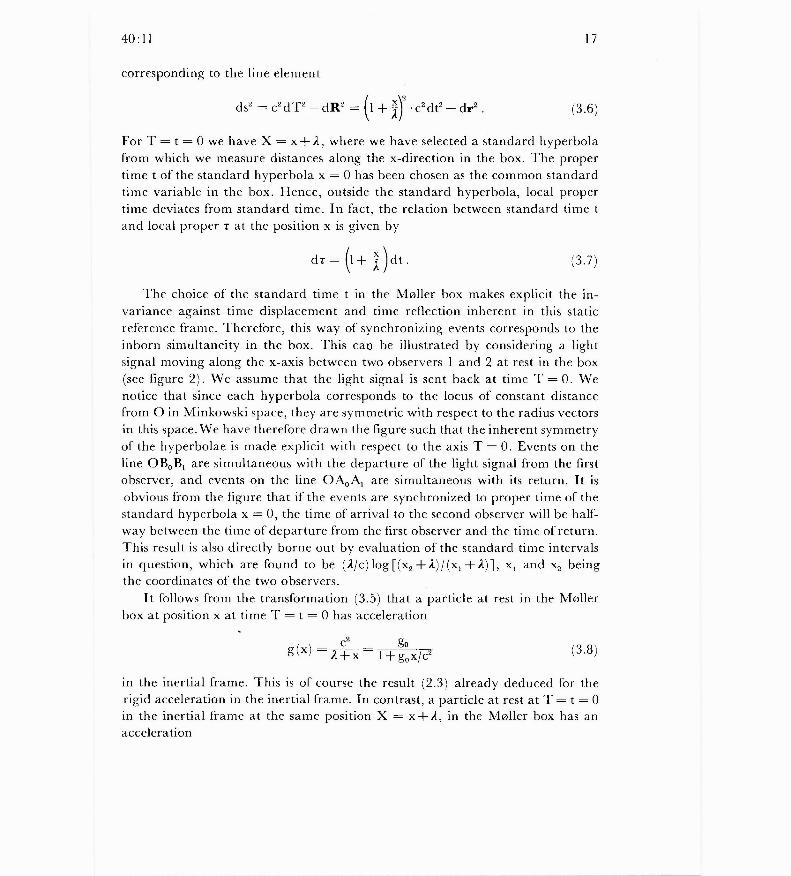
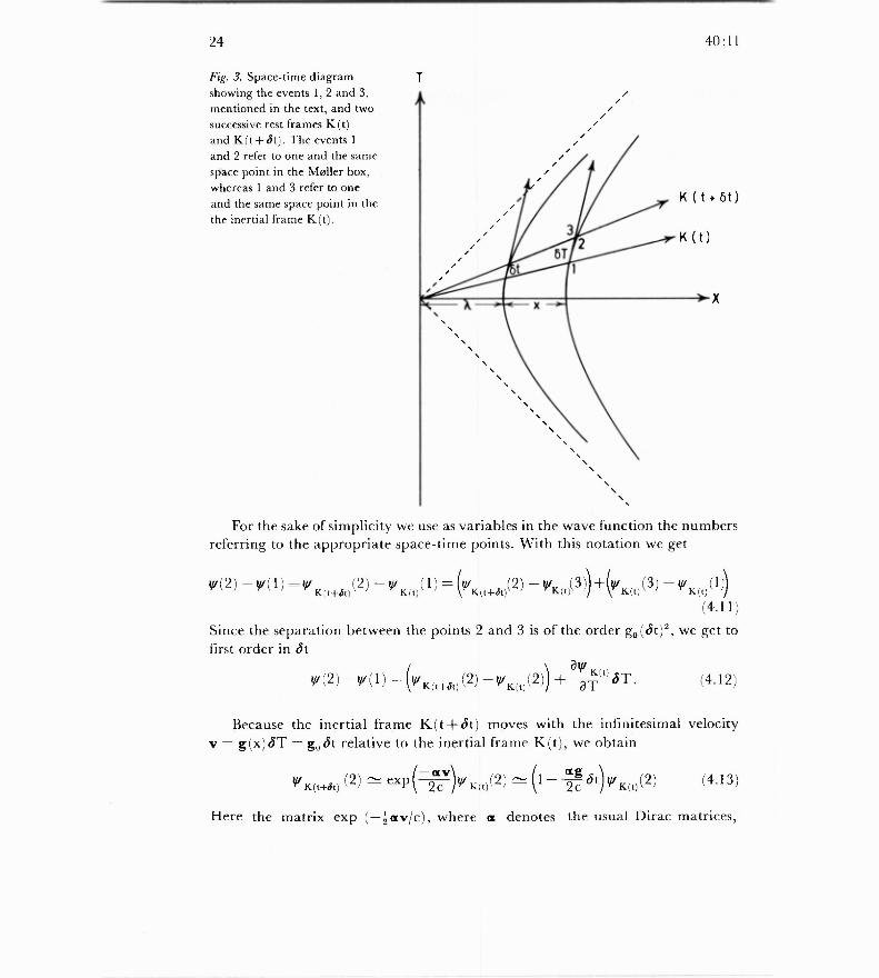
The time variation of v(t) is due partly to the change of inertial frame K(t)with time and partly to the intrinsic time variation of the state. In order to findthe change with time, t, of the wave function at a fixed space point in the box,let us consider the three events pictured in Fig. 3. Here the events 1 and 2 referto one and the same space point in the box, but are separated by the time intervalåt in this frame. Similarly 2 and 3 are simultaneous in the box, whereas 1 and 3refer to one and the same space point in the inertial frame K(t), but are separatedby the time interval 8T in this frame.

aw(rn> re) 2Ze2

24

40:11

Fig. 3. Space-time diagramshowing the events 1, 2 and 3,mentioned in the text, and twosuccessive rest frames K(t)and K(t+St). The events 1and 2 refer to one and the samespace point in the Møller box,whereas 1 and 3 refer to oneand the same space point in thethe inertial frame K(t).

T

For the sake of simplicity we use as variables in the wave function the numbersreferring to the appropriate space-time points. With this notation we get

w( 2 ) —w(1) w K(t+at, (2) — V k(t) (1) =(VK(t+bt)(2) —wK(t)(3))+(K(t) (3) — li(t) (1)

(4.11)

Since the separation between the points 2 and 3 is of the order g o (öt) 2 , we get tofirst order in 8t

w (2)-4^(1)=(w K+Ö (2)—w (2))+^^K(t) aT.t) K(t) ÔT

Because the inertial frame K(t +60 moves with the infinitesimal velocityy = g(x)c5T = g„&t relative to the inertial frame K(t), we obtain

^K(t+at) ( 2 ) ^ exp ( 2 c)W K(t) (2) (1— 2g ot)w K(t) (2) (4.13)

Here the matrix exp (— Zav/c), where a denotes the usual Dirac matrices,

(4.12)

40:11 25

transforms the wave function from the inertial frame K(t) to K(t+åt). Combining(4.10), (4.12) and (4.13), we obtain

ihåw= - ih g0 yi+(1+ )ih å = ih 7°yi+(1+ )H . (4.14)

Here Hn is the Dirac Hamiltonian in the inertial frame K(t),

Hn = cot (la +4AK) , ))+ß1nc2 — x)c), (4.15)

where (NPK (, ), Ax(t) ) is the four-potential in the frame K(t), and where the electroncharge is —e. The Møller box coincides with K(t) at time t, and therefore

p = — ifiVr , (4.16)

where r denotes the spatial coordinates in the box. From the equations (4.14)-(4.16) it follows that the Dirac equation in the Møller box takes the form, validto all orders in 1/A,

ih = [(l+)HI)+HD(l+)]w. (4.17)

From eq. (4.17) one may derive the continuity equation

åt (v+v) +di ,. (w + (1 + )coop) = 0 . (4.18)

'hherefore, the quantity (— eyi +yi) is the charge density in the Møller box and(—ev +(l +x/A)acyi) is the charge current density.

In order to apply the Dirac equation to a hydrogen atom with the nucleus atrest at r = 0, we have to find the potentials WK)r) and AK),) generated by thenucleus. Because the inertial frame K(t) is the momentary rest frame of thenucleus at time t, the retarded potentials are to first order in the accelerationgiven by (cf. ref. 12, p. 167)

ZeZe d2r^PK^t ) = r + 2c2 dT2 >

AK(,) = 0,

where r = ^r e —r,j and d2 r/dT2 refers to the inertial frame K(t), i.e.2

d r __ >;o' (re —rte)dT2 r

(4.19)

(4.20)

Thus we obtain

26 40:11

Sk i t, — ^ r —r (1 2c2 )'e „

Ze go • (re —re)

(4.21)0.

From (4.15) and (4.17) we then get

t =}2 (1+ ^ ̂ ( ca • p o --ßIn e c22) + (ca • R• -}-ßmE,c2) (1-}- ^'^ — eT(re>r„)} tit

l (4.22)Here the potential

(rei rn) — l +xe^ )tfl,:,t) (re;rn)

is seen to be identical with the electrostatic potential in the Møller box as given,to first order in 1/A, by (3.15). The Hamilton in (4.22) is just what one wouldobtain by simply replacing the square root in the Hamiltonian (4.6) by

(ca.P e +ßtnec2).Since (—eyi +yi) is the charge density of the electron in the atom, we can

immediately write down the expectation value, F,„ of the reaction force on thenucleus from the electron in a stationary state. By steps analogous to those of eq.(4.7), we obtain

F,, = —< yratV(rn ; re)Ze— aXt — I r,=o

yr >=

=-<yrhireAire —r„ Yi>+<W

ayo (re >rn)^w>a xe

(4.23)

=—<w Z e2 'Pe+ßntec2 — ^re —rel >-2

=-•-• — (me— B go).

Thus the total force required to keep the atom at rest is given by the expression(4.5), where B, the binding energy of the electron, now includes spin-orbit coupl-ing, the Darwin term and all other effects contained in the Dirac Hamiltonian.

It is also possible to demonstrate equivalence for a hydrogen-like atom de-scribed by the Klein-Gordon equation. Since the argumentation is somewhatdifferent from the cases considered so far, the Klein-Gordon equation is treatedseparately in appendix C.

(4.24)

40:11 27

Thomas-Fermi atom

In the previous analysis we have considered equivalence for electrostatic energiesand kinetic energies of a single particle bound in an atom. When we turn to moregeneral systems, consisting of several moving charged particles, one might attemptto base the discussion on a mechanical description in terms of the coordinatesand velocities of the particles only. It has turned out, however, that this descrip-tion can in general only be carried to terms proportional to 1/c 2 , within an expan-

sion in powers of 1/c. The corresponding Lagrangian is the familiar one intro-

duced by Darwin (cf. Landau and Lifshitz 12 ). Equivalence may be demonstratedwithin this scheme, but a strong limitation is then imposed on the internalvelocities of the system as well as on the velocity belonging to Lorentz transfor-mations. Such limitations are avoided in a self-consistent description of the system,in which each particle interacts with a common four-potential, the latter beinggenerated by the particles themselves. As a first step towards such general dynam-

ical descriptions we shall study equivalence for the simple case of a non-relati-

vistic Thomas-Fermi atom.The first step is to estab lish, within the Møller box, the equilibrium condition

for the electron distribution in an atom, the nucleus of which is at rest at r„ = 0.The local Fermi momentum of a degenerate electron gas is

pF(r) (37z.2)113hn113(r), (4.25)

where n(r) is the density of electrons. "Thus, the electron charge density is

Qe (r) =—en(r), (4.26)

and the total charge density of the system is

Q (r) =ee (r)+Ze å (r—r„) . (4.27)

For a free atom at rest, the total Hamiltonian of the system then takes on thefamiliar form (cf. Gombås14)

H= d 3 r(inc2 + 3 11(11-1 ))11(r) + d 3 r Zeee(r) + 1Jd 3 rJd3 r' ee r e(r ) , (4.28) ^ ^r' ^

where m is the electron mass.For the total electric potential tp(r), generated by the charge distribution

(4.27), we have according to (3.15)

q)(r) _ 1 d3r, ^(r , ) ^ +

+ xx,2A )'(4.29)

The effective Lagrangian for the individual electron, moving in the total

28

40:11

potential tp, is given by (3.21), and the corresponding Hamiltonian for a singleelectron is to lowest order in v2/c2

H e = (l+)1)(mc2+ pm )—eto (r) . (4.30)

All electron states up to the Fermi momentum p F (r) are occupied, and in equilib-rium the maximum energy, Emax , that an electron can have at any point, isconstant throughout the atom

(l+)(mc2 +p(r))_ e(r) = E max , (4.31)

where we have introduced the potential

u(r ) = p(r)

= (37t2)" h2 n2 / 3 (r) . (4.32)2m 2m

Combining (4.32) with the generalized Poisson equation (3.14), one may obtainthe Thomas-Fermi equation in the Møller box.

In order to derive the reaction force on the nucleus due to the electrons, wenote that from the potential (4.29), one obtains as a generalization of the relation(3.17)

Jd2rQ(r) ôx l d r rr'^aw(r) 1 s (r )e(r')

(4.33)

This relation is valid for any static charge distribution and may in particular beapplied to the charge distribution en (r) of the nucleus and the potential to n that

it generates

Jd3rn(r)

ô å (r) = 22 Jd3rJd3r' en

1 (r ) er (r') (4.34)

Next, we write the total potential in (4.33) as

tP(r ) =tPn (r) +Te(r), (4.35)

where ye (r) is the potential generated by electron charge distribution ee (r) .Subtracting (4.34) from (4.33) we obtain

Jd3ren(r) å(r) +Id3 r en (r)

a a(r) =

= l d 3 rf d3r' en (r')ee(r)+ 1 Jcl3rJd3r' ee (r) ee(r')

J

(4.36)

40:11 29

In this relation we may approximate the charge distribution en (r) of the nucleusby a delta function in accordance with (4.27). For the reaction force on thenucleus from the electron distribution we thus get

Fx=— Ze açe (r) aX r=0

Jd3ree(r) aa (r) d3 r

Zr P (r)

21^fd3fd3r ee

1(̂ )P^ (^ ') (4.37)

Expressing the potential yo in terms of ft, cf. the equilibrium condition (4.31), andusing (4.32), we find

fd3re(r) ôx —1d3 r n (r) ax {(1+R)(p(r) -1-me2)}

_— d 3 rn (r)1(u(r)+ mc2) +(1 + 3n2(h2 ,u)3/2

= -Jd3 r n (r) (me ^- µ(r)) , (4.38)

where the last equation follows by partial integration. Inserting this expressionin (4.37), the reaction force, Fx , becomes:

Fx =— H go =— I 11Tm—B) go^ (4.39)

where H is the Thomas-Fermi Hamiltonian (4.28) and N the total number ofelectrons. For the total force required to keep the atom at rest, we thus againobtain the expression (4.5), where B is the binding energy of the Thomas-Fermiatom.

§5. Conclusions and General Outlook

In the previous chapters we have verified that there is equivalence betweeninertial mass and self-energy. The study was performed in considerable detail,including electrostatic interactions and kinetic energies, for hydrogen-like systemsand the Thomas-Fermi model, within both classical mechanics and relativisticquantum mechanics. Moreover, there was detailed equivalence, i.e. equivalencefor each term and for each element of the interaction energy. It was not necessaryfor the treatment that the system were stable. Without doubt, these are satisfactoryresults since they imply that all terms of a calculation of self-energies have aseparate and simple significance.

aulax

30 40:11

The equivalence could be made specific in terms of the basic equation ofmotion (2.12) for a charged, composite system, g e M = gE,„t(r0,t). Thus, not

only did the mass M contain detailed equivalence, but also the system, and itsacceleration, could be represented by one point: the centre of charge r,. Higherorder terms, like radiation damping, may afterwards be built into the aboveequation of motion. In connection with these results we showed that there is anerror in the standard Born-Heitler calculation of self-mass from total self-force.As to the conventional formulae for self-momentum and self-energy, i.e. (1.8) and(1.9), we found that they resulted from an unwarranted variation of a constantterm in the Lagrangian (2.15), and therefore could not be compared with theproper momenta and energies. It was apparent that if one kept to a Lagrangianformulation in describing a system, the undesirable expressions (1.8) arid (1.9)were avoided, the need for Poincaré stresses did not arise, and detailed equiva-lence was explicit.

There is a more general background to our work, concerned with the con-sistency and aim of the description. As promised in the brief introductory remarksin §1, we shall now discuss this background.

We have been concerned with composite systems, and with their primaryproperty, i.e. their mass. It was supposed that we can speak consistently aboutsuch systems. But already in the wording composite systems it is implicit that asimpler concept exists. In point of fact, we have an idealized concept, that of aparticle, sometimes referred to as an elementary particle, or a point particle. Fromold, a particle is conceived as an unchangeable building stone of matter. On the

one hand, we then visualize a composite system as a swarm of particles interactingwith each other. On the other hand, we have to compare the properties of thisswarm with the properties of one particle, asking for the likeness between thetwo, as well as for their difference in behaviour.

For the purpose of this comparison, consider a composite system, be it amolecule, a liquid drop, a crystal, or an atomic nucleus, and note the following.If we act upon the system by means of comparatively weak forces, the forcesvarying sufficiently slowly in space and time, then the behaviour of the systemwill be as if it were a particle. This means that it has a certain mass, charge,inner angular momentum, magnetic dipole moment, etc. It can possibly berepresented as a point in space as was shown in the equation of motion (2.12),just in the way a particle — if we are cautious — can possibly be described as apoint in space. By acting on the system with such moderate forces, we can measurethe properties of the system, properties which are conserved when the systemremains isolated. In this comparison to a point particle we need not require thatthe system be absolutely stable when isolated. We can allow it to be unstable,

40:11 31

like a.uranium nucleus with a probability of fissioning, or like a liquid drop whichmay evaporate. In such cases we can think of it as having conservation withinsufficiently short time intervals, or with a certain width of its energy. Note inthis connection that, in the main, it is permissible to use classical mechanics aswell as quantum theory in the description of the system, although, of course,quantum mechanics will give a more precise account of the physical properties.

Thus, in the limiting case of weak and slowly varying external fields, we find

that we must be able to describe a composite system and a particle in a likemanner. It lies near at hand to demand that we are also able to account for their

properties in a like manner. In a way, this hypothesis corresponds to the historicaldevelopment of particle physics where successively, molecules, atoms, and atomicnuclei, etc., have been described as elementary particles. But it is more essentialthat actual calculations of basic properties of systems comply with our demand,in so far as we are able to calculate these properties. Correspondingly, the problemof equivalence of mass and energy must be our primary concern.

Consider then calculations of self-energies and self-masses for, on the onehand, composite systems, and, on the other hand, particles. In the case of com-posite systems this calculation is prescribed: we treat its constituents, e.g., elec-trons and atomic nuclei, as elementary particles, and only their interactions andtheir motion contribute to the additional self-energy and mass. It is importantto notice that constituents of a composite system — constituents like the aboveatomic nuclei — often can be regarded as composite systems themselves, and sothe division into constituents can be somewhat free. This possibility of a variabledivision into constituents leads to the further expectation that each separate inter-action contribution, or kinetic energy contribution, should show equivalence.We described this as the demand of detailed equivalence, and we verified that it

is fulfilled.If we demand a systematic account, the above ought to be compared with

self-energies for particles, such as the self-energy of an electron. The latter conceptis not quite simple, however, and that mainly on three counts. First, the basicmethod of finding self-energies belongs primarily to composite systems, and we

can merely maintain that the proper procedure for a supposedly elementaryparticle must not be in discord with the former. Second, the leading term in theelectron self-energy is apparently divergent, whereas the physically observableparts of the self-energy, like the Lamb effect, appear only in higher order termsin expansions in powers of 1/c. But our primary concern, for composite systems,was not to evaluate cumbersome higher order terms. Third, there is an interest-ing complication because of the spin and magnetic moment of the electron ; inorder to make a comparison, one must first analyse composite systems with spin,or inner angular momentum. We have made this study and found that a classical

32 40:11

system with spin must be described by at least two points, the centre of motionand the centre of charge. An account of these questions will be given in a separatepublication.

Acknowledgments

This paper has been under way during one decade. The contents of it, and itsaim, has changed considerably in that period. Part of the subject, systems withspin, has been reserved for a future publication. We are grateful to many friendsfor debates on equivalence as well as subjects akin to it. We have, in particular,profited much from discussions with E. Eilertsen, P. Kristensen, Vibeke Nielsen,W. J. Swiatecki, and A. Winther.

We are especially indebted to Lise Madsen for competent and careful pre-paration of the paper.

40:11 33

Appendix A

Electrodynamics in Møller Box

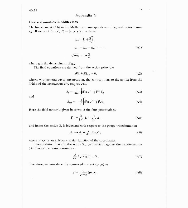
The line element (3.6) in the Møller box corresponds to a diagonal metric tensorg ;k . If we put (x°, x 1, x2, x3 ) = (ct,x,y,z), we have

goo =(i+)2,

g11 - g22 — g33 — l , (Al)

A/—g= 1+^,

where g is the determinant of gik .The field equations are derived from the action principle

(SS,

where, with general covariant notation,field and the interaction are, respectively,

6S,„ = 0,

the contributions to the action

(A2)

from the

and

— 1617rc

f d4x^ F' F, (A3)Sr

S int — C2 f d4 x1/ —g (A4)

Here the field tensor is given in terms of the four-potentials by

__ aFik ax'

a(A5)Ak A i,

_axk

and hence the action S 1 is invariant with respect to the gauge transformation

A,—> A+ a i A (r,t)T ô

where A(r, t) is an arbitrary scalar function of the coordinates.The condition that also the action S, nt be invariant against the transformation

(A6) yields the conservation law

ax' (A/ gJ') = 0 .

Therefore, we introduce the conserved current (ec, s) as

l' = ^ g

(e c , s ) ,

(A6)

(A7)

(A8)

34

40:11

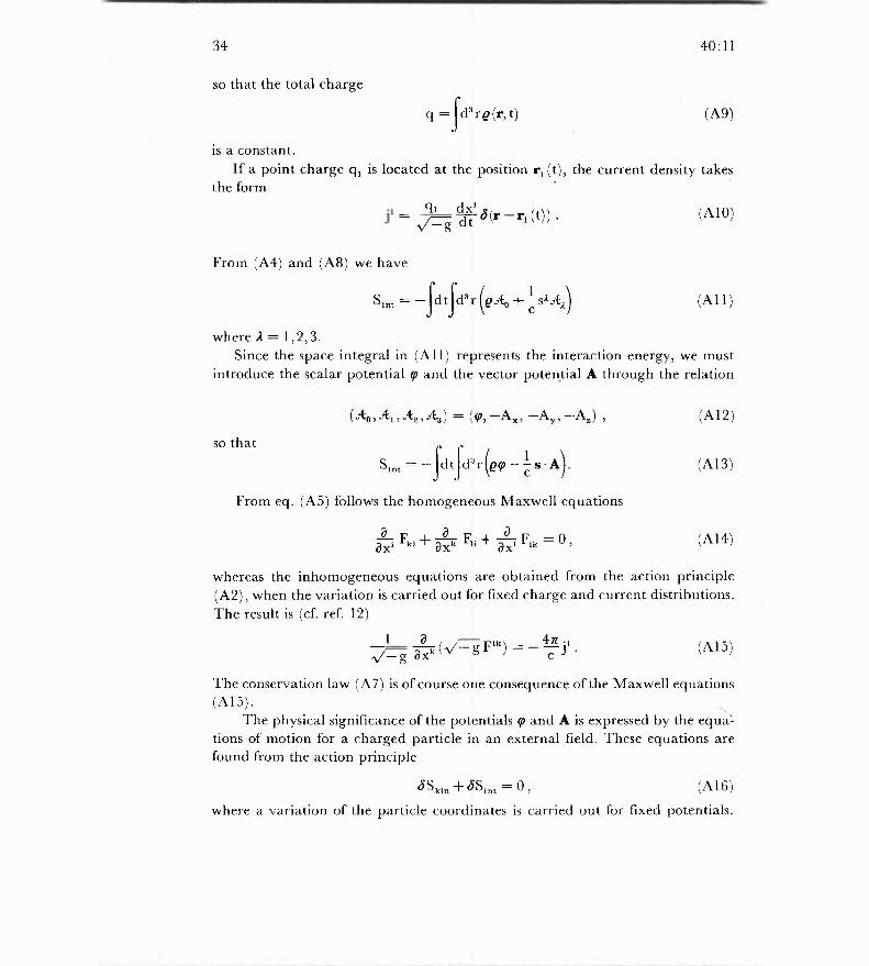
so that the total charge

q =Jd3re(r,t)

is a constant.If a point charge q l is located at the position ri (t), the current density takes

the form

qidxi 8 (r—ri (t)) .^/—gdt

From (A4) and (A8) we have

(('' 1 lS ant

=— dtJd 3 r (e +sxtk (All)

where .l = 1,2,3.Since the space integral in (All) represents the interaction energy, we must

introduce the scalar potential ç and the vector potential A through the relation

(^o,.4i,.42,.43) = (W, —Ax, —A —Az) , (Al2)

so that ('

S int = —Jdt f d ; r(e^— s • A). (A13)

From eq. (A5) follows the homogeneous Maxwell equations

Øx` Fk ' + xk F. + 8x' Fik — 08

whereas the inhomogeneous equations are obtained from the action principle(A2), when the variation is carried out for fixed charge and current distributions.The result is (cf. ref. 12)

-\/—g aXk( 3_ gFik) =- 4̂ j. (A15)

The conservation law (A7) is of course one consequence of the Maxwell equations(A15).

The physical significance of the potentials ç and A is expressed by the equaltions of motion for a charged particle in an external field. These equations arefound from the action principle

(A9)

(A10)

(A14)

aSkin + ôS int = 0 , (A16)

where a variation of the particle coordinates is carried out for fixed potentials.

40:11 35

Here

Ski n =— mc2Jdt^(1 } )z— v2 }1/2' (A17)

S,,1 = —Jdtq{rp(r(t)) — A(r(t)}, (A18),

where m is the mass of the particle and q its charge. The corresponding Lagrangian

is

L=—mc2 (1+ ) -- 1

—q^p(rt)+g v • A(r,t), (A19)2 2 /2

and hence the equations of motion become

—m(1 +x/.î)go +!^ E + vc XB ,d `1 dt {(1+x/2)

mv

2— v2/c2 {1/2 — {(1 +x/Å)2 —v2/c2^1/2 (A20)

where we have introduced the electromagnetic fields

E= —V^p—^ å—̀̂, (A21)

B = V x A . (A22)

In terms of these quantities the field action (A3) takes the simple form

S1 = nJdtJd3r(1 +x/ .1 (1+x/.1)B) . (A23)

It can be convenient to express the Maxwell equations (A14) and (A15) inthe following three-dimensional notation

div B = 0 ,

rot E _ — caB at ,

(A24)div D = 4ne ,

rot H=1 aD+ 4n sc at c

where we have introduced the abbreviations

1 (A25)D 1+ x/.lE ,

H = (1 + 1)B. (A26)

36

40:11

Appendix B

Static Potentials in Møller Box

In this appendix we derive the potential generated by a charge at rest in the box.By introducing (A21) and (A25) into (A24), one obtains the generalized Poissonequation for the potential tp,

d^— ^

+

x å^=-4ng,(1+ 8(r—rt) ,

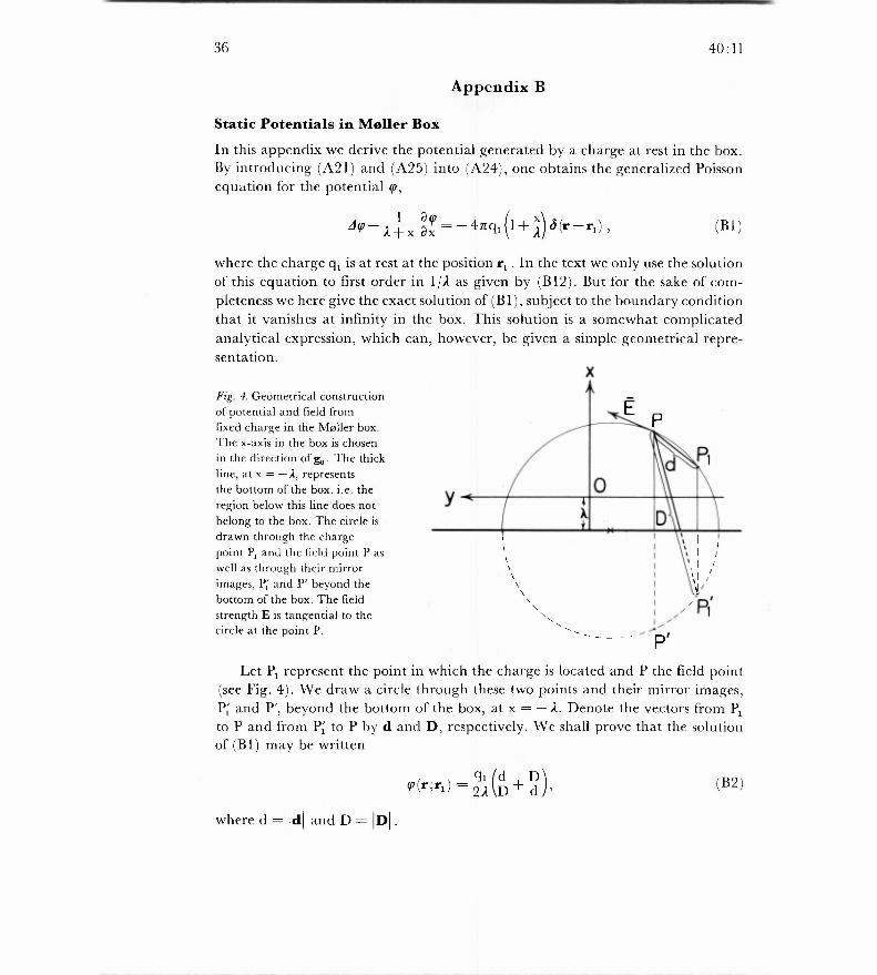
where the charge q, is at rest at the position r, . In the text we only use the solutionof this equation to first order in 11A as given by (B12). But for the sake of com-pleteness we here give the exact solution of (B1), subject to the boundary conditionthat it vanishes at infinity in the box. This solution is a somewhat complicatedanalytical expression, which can, however, be given a simple geometrical repre-sentation.

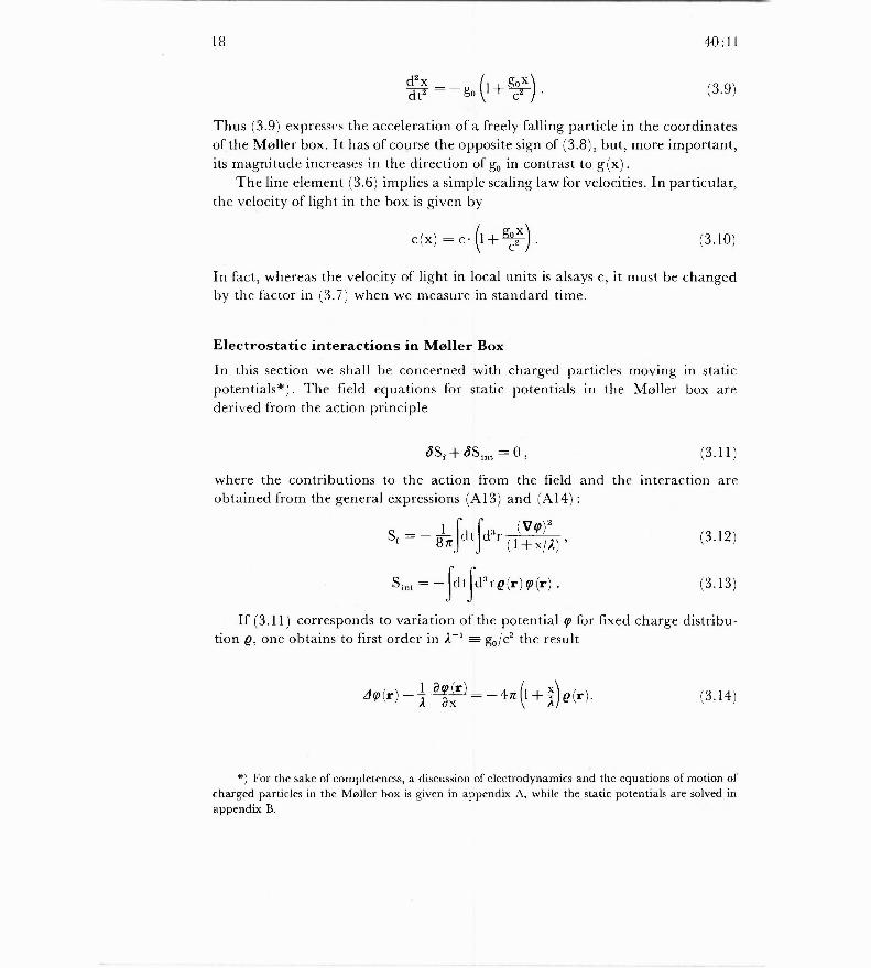
Fig. 4. Geometrical constructionof potential and field fromfixed charge in the Møller box.The x-axis in the box is chosenin the direction of go . The thickline, at x = —A, representsthe bottom of the box. i.e. theregion below this line does notbelong to the box. The circle isdrawn through the chargepoint P, and the field point P aswell as through their mirrorimages, Pi and P' beyond thebottom of the box. The fieldstrength E is tangential to thecircle at the point P.

P"Let P, represent the point in which the charge is located and P the field point

(see Fig. 4). We draw a circle through these two points and their mirror images,P; and P', beyond the bottom of the box, at x = —2. Denote the vectors from P,to P and from P; to P by d and D, respectively. We shall prove that the solutionof (B1) may be written

q^( d Dq)(r;r1) =2^ D + d °

(B1)

(B2)

DI.where d = and D =

40:11 37

The right hand side of (B2) tends to the constant q,/A. at infinity and at thebottom of the box. It is seen from Fig. 4 that d and D are given by

d - {(x x1)2+ (y y1)2 + lz - z1)2r2

D={(x+.l+x1+11)2+ (y- y1)2 +(z- z1)2}1/2.

In order to show that (B2) is a solution of (B1), we observe that the Laplacianacting on d/D becomes

Ad = 1 . 4d+dd1+2(V

d)•(V^

=- 4nd8(D)+d1D D3+ 4(å+A)2

(B5)

and similarly

d D = -4nD8(d)+dD d3 4(Dd3^)2.

Furthermore,

1 ô d 1x—x1 dx--).+x,+2

.1 +x ax D .l +x ( dD D3 )'

1 8 D 1 (x-f-xl +. D (x+,) — (xl +.l).1 +x ax d .1 +x dD d3 )'

Finally, making use of the relation

D2 —d2 = 4(x+ 2) (x, +.1) , (B8)

we obtain

(zi

x i3x) (Dd

D ) =- 4nh(D8(d)+d8(D)) .

Since 8(D) vanishes everywhere within the box, we have verified that, apartfrom an additive constant, (B2) is the solution of (B1) with the desired boundarycondition. It is easily seen that the electric field E at the point P is tangential tothe circle and of magnitude

E (P) = q, (1+ 1)(d2 — D2). (B10)

Incidentally it may be remarked that a light ray, sent from the point P, to thepoint P, travels along the circle shown on the figure.

In order to obtain the potential to first order in 11A we expand as follows

(B3)

(B4)

(B6)

(B7)

(B9)

38 40:11

D= 2^1+x, +x . . . . (B11)

Hence the potential becomes

Dx

q ^

l + T x i )

`^— 2.1 d ir—rd 2.i '

which is the form used in the text.The above result for the potential may also be derived by transforming the

potentials, generated by a charge in hyperbolic motion, from the inertial frameto the Møller box and performing a gauge transformation. The potentials in theinertial frame were originally derived by Borneo

(B12)

40:11 39

Appendix C

Klein-Gordon Equation in Møller Box

Let K(t) denote the particular inertial frame which coincides with the Møllerbox at time t. In this frame, the Klein-Gordon equation for a spinless particleof charge q and mass m in an external potential .it may be written as

(P, _q Ai) (P1_1)

(T) = m2c2WK(t((T)

(C1)

where WK(t) (T), the wave function in the frame K(t), is a scalar quantity. With

the identification

P = ih ax"

and imposing the Lorentz condition we obtain

C12(_h2 D _2ihkai +

z

1 A. 1 A ,)y^K(t (T) = 2 ezWK(t)(T). (C3)2

We now notice that the wave function in the Møller box y(t) is equal to the wave

function WK (t) (T)

W( t) = WK ( t ) (T) •

Moreover, since WK(,) is a scalar, the product A l aVx(1) l ax' is an invariant.

Therefore the Klein-Gordon equation in the Møller box is simply obtained byexpressing this invariant and the d'Alembertian in non-Euclidean coordinates.For the latter operator we have the general expression (cf. ref. 12, §86)

1 a ;k a q_—g ax' ,3

—g gik .

With the metric (Al) in the Møller box, this operator becomes

1 1 a2 1 aq _ (l

+x/2) 2 c2 ate — (d+ A+ x ax

z(1-2x/.1)

c2 aa2 —(d+-} ax ,

where the last expression is valid to first order in 1/.1. We shall only considerthe case of a static potential in the Møller box, i. e. = (9, 0, 0, 0) . Hence we

obtain

a = goo ^ ao=)

1 2 ^ 1 a (1 -2x/a.) ^ ^ åtax ax (1+ x/).)2 c at

(C2)

(C4)

(C5)

(C6)

(C7)

40 40:11

Similarly,

.A'. =g°° (1-2x/Å) (v2. (C8)

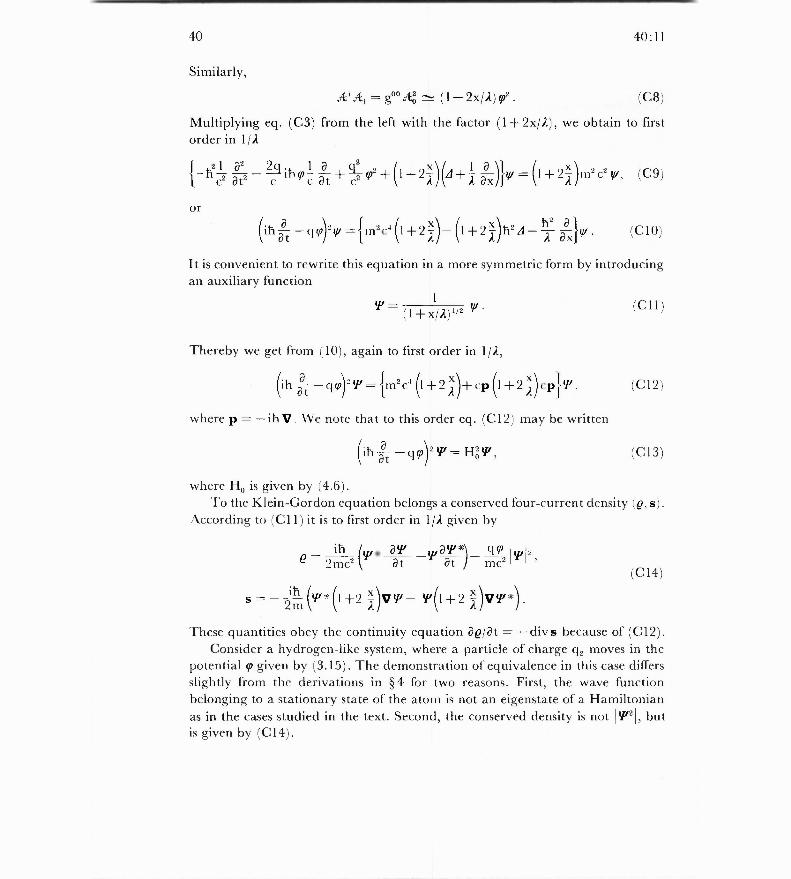
Multiplying eq. (C3) from the left with the factor (1+ 2x/.1), we obtain to firstorder in 1/A

{

,2 1 a2 c2

ate— ihço-

ôt + 29

2 + ( 1 +23)(61+1 ){yi=(1 b2-)m 2 c2 y/ , (C9)

ora

( W T.ihôt —qy')^ = m2ca (1+ 2^)—( 1 +2^ h2 d— ôx .

It is convenient to rewrite this equation in a more symmetric form by introducingan auxiliary function

_ 1 (l+ x/.i)1/2 V-

Thereby we get from (10), again to first order in 11A,

(ih — q = {in2c4 (1 + 2 cp (I + 2 (C12)

where p = —ih V. We note that to this order eq. (C12) may be written

(ih at — q(P)2`y = Hô`y,

where H„ is given by (4.6).To the Klein-Gordon equation belongs a conserved four-current density (O, s) .

According to (C11) it is to first order in 1/A given by

ih2

(^ ^ aY! _Yr)_ e mc2 Øt at mc21

s=— 2m (gi * (1 +2 ^)V`y — y^ ( 1 +2 ^)VYr*).These quantities obey the continuity equation ae/at= —divs because of (C12).

Consider a hydrogen-like system, where a particle of charge q 2 moves in thepotential tp given by (3.15). The demonstration of equivalence in this case differsslightly from the derivations in §4 for two reasons. First, the wave functionbelonging to a stationary state of the atom is not an eigenstate of a Hamiltonianas in the cases studied in the text. Second, the conserved density is not VI, butis given by (C14).

(C10)

(C11)

(C13)

(C14)

40:11 41

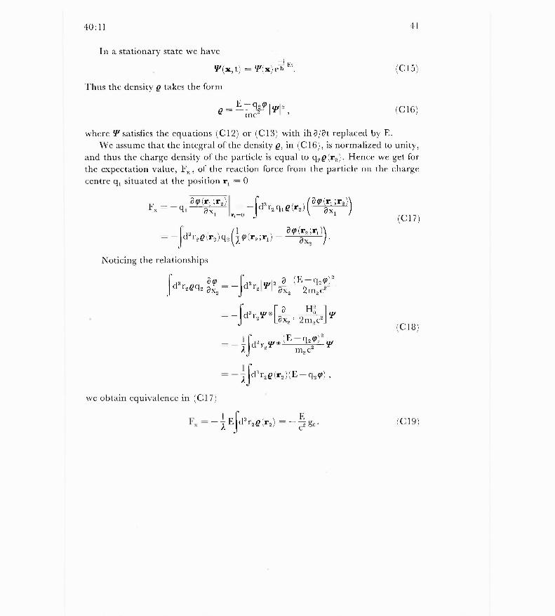
In a stationary state we have

W(X t) = ,(x)eE Ei

Thus the density P takes the form

P— E — q2 ^F ,j, 2

mc

where VI satisfies the equations (C12) or (C13) with iha/at replaced by E.We assume that the integral of the density g, in (C16), is normalized to unity,

and thus the charge density of the particle is equal to g 2 g(r2 ). Hence we get forthe expectation value, Fx , of the reaction force from the particle on the charge

centre q 1 situated at the position r = 0

Fx = —g 1 axlaw(r,;r2)

r-0= d3r2g^^(r2)( ^G(

i ^ 2— axi

ô r•r )

3 (1 aW(r2;r11\_ — d ' r2P(r2) g2 ^^(r2^ri, ax2 f •

Noticing the relationships

d3r2 gg 2 L92= —fd3r2 Y' 2 a (E—g29)2ax, 2 m 2 c2

= —3 ^d r2 Y^

a1-120 w

(C18)L ax2 ' 2m2c2 J

=—^ mJd3r V* (E

g^9)2y,2 2

2

— 9id3r2C(r2)(E—q2v) e

we obtain equivalence in (C17)

— ^ EJ

d3r2P(r2) = — E go•

(C17)

(C19)

42 40:11

References1.Jackson, J. D., Classical Electrodynamics, Chapter 17, Wiley, New York (1962).2. Einstein, A., Ann. d. Phys. 17, 891 (1905), Ann. d. Phys. 18, 639 (1905).

Reprinted in English translation in "The Principle of Relativity", Dover Publications (1952).3. v. Laue, M., Inertia and Energy, in "Albert Einstein, Philosopher-Scientist", (Ed. A. Schilpp)

The Library of Living Philosophers, Evanstone, Illinois (1949).4. Jammer, M., Concepts of Mass, Chapter 11, Harvard University Press (1961).5. Lorentz, H. A., The Theory of Electrons, Teubner Verlag, Leipzig (1916). Reprinted in Dover

Publications (1952).6. Pais, A., Developments in the Theory of the Electron. Institute for Advanced Studies and

Princeton University (1948).7. Feynman, R. P., Lectures on Physics II (Chapt. 28), Addison-Wesley, Reading, Mass. (1964).8. Becker, R. and Sauter, F., Theorie der Elektrizität, Teubner Verlag, Stuttgart (1957).9. Rohrlich, F., Am. J. Phys. 28, 634 (1960), Ibid. 38, 1310 (1970), and

Classical Charged Particles, Addison-Wesley, Reading, Mass. (1965).10. Born, M., Ann. d. Phys. 30, 1 and 840 (1909).11. Heitler, W., The Quantum Theory of Radiation, Oxford University Press, Oxford (1954).12. Landau, L. and Lifshitz, I. M., Classical Theory of Fields, 3. ed. Pergamon Press, Oxford, New

York (1973)13. Møller, C., The Theory of Relativity, Oxford Universi ty Press, Oxford (1972).14. Gombäs, P., Die Statistische Theorie des Atoms und ihre Anwendungen, Springer Verlag,

Wien (1969).

Indleveret til Selskabet december 1981.Færdig fra trykkeriet juni 1982