sensor fusion with coordinated mobile robots
TRANSCRIPT
Sensor Fusion with Coordinated Mobile Robots
Examensarbete utfört i Reglerteknik vid Tekniska Högskolan i Linköping
av
Per Holmberg
LiTH-ISY-EX-3387-2003
Linköping 2003
Sensor Fusion with Coordinated Mobile Robots
Examensarbete utfört i Reglerteknik vid Tekniska Högskolan i Linköping
av
Per Holmberg
LiTH-ISY-EX-3387-2003
Handledare: Ph.D. Jonas Nygårds, FOI
Prof. Åke Wernersson, FOI Lic. Rickard Karlsson, ISY
Examinator:
Ph.D. Mikael Norrlöf, ISY
Avdelning, Institution Division, Department Institutionen för Systemteknik 581 83 LINKÖPING
Datum Date 2003-05-16
Språk Language
Rapporttyp Report category
ISBN
Svenska/Swedish X Engelska/English
Licentiatavhandling X Examensarbete
ISRN LITH-ISY-EX-3387-2003
C-uppsats D-uppsats
Serietitel och serienummer Title of series, numbering
ISSN
Övrig rapport
____________
URL för elektronisk version http://www.ep.liu.se/exjobb/isy/2003/3387
Titel Title
Sensorfusion med koordinerade mobila robotar Sensor Fusion with Coordinated Mobile Robots
Författare Author
Per Holmberg
Sammanfattning Abstract Robust localization is a prerequisite for mobile robot autonomy. In many situations the GPS signal is not available and thus an additional localization system is required. A simple approach is to apply localization based on dead reckoning by use of wheel encoders but it results in large estimation errors. With exteroceptive sensors such as a laser range finder natural landmarks in the environment of the robot can be extracted from raw range data. Landmarks are extracted with the Hough transform and a recursive line segment algorithm. By applying data association and Kalman filtering along with process models the landmarks can be used in combination with wheel encoders for estimating the global position of the robot. If several robots can cooperate better position estimates are to be expected because robots can be seen as mobile landmarks and one robot can supervise the movement of another. The centralized Kalman filter presented in this master thesis systematically treats robots and extracted landmarks such that benefits from several robots are utilized. Experiments in different indoor environments with two different robots show that long distances can be traveled while the positional uncertainty is kept low. The benefit from cooperating robots in the sense of reduced positional uncertainty is also shown in an experiment. Except for localization algorithms a typical autonomous robot task in the form of change detection is solved. The change detection method, which requires robust localization, is aimed to be used for surveillance. The implemented algorithm accounts for measurement- and positional uncertainty when determining whether something in the environment has changed. Consecutive true changes as well as sporadic false changes are detected in an illustrative experiment. Nyckelord Keyword Kalman filter, extended Kalman filter, estimation, mobile autonomous robots, cooperative localization, laser range finder, encoder, change detection
Abstract Robust localization is a prerequisite for mobile robot autonomy. In many situations the GPS signal is not available and thus an additional localization system is required. A simple approach is to apply localization based on dead reckoning by use of wheel encoders but it results in large estimation errors. With exteroceptive sensors such as a laser range finder natural landmarks in the environment of the robot can be extracted from raw range data. Landmarks are extracted with the Hough transform and a recursive line segment algorithm. By applying data association and Kalman filtering along with process models the landmarks can be used in combination with wheel encoders for estimating the global position of the robot. If several robots can cooperate better position estimates are to be expected because robots can be seen as mobile landmarks and one robot can supervise the movement of another. The centralized Kalman filter presented in this master thesis systematically treats robots and extracted landmarks such that benefits from several robots are utilized. Experiments in different indoor environments with two different robots show that long distances can be traveled while the positional uncertainty is kept low. The benefit from cooperating robots in the sense of reduced positional uncertainty is also shown in an experiment. Except for localization algorithms a typical autonomous robot task in the form of change detection is solved. The change detection method, which requires robust localization, is aimed to be used for surveillance. The implemented algorithm accounts for measurement- and positional uncertainty when determining whether something in the environment has changed. Consecutive true changes as well as sporadic false changes are detected in an illustrative experiment.

Acknowledgments This master thesis was performed at the Division of Command and Control Systems, FOI in Linköping during the winter 2002/2003. I would like to thank FOI for the opportunity to do my master thesis in an exciting research area. I especially owe gratitude to Ph.D. Jonas Nygårds and Prof. Åke Wernersson whom supervised the work throughout the thesis. I would also like to thank Lic. Rickard Karlsson and Ph.D. Mikael Norrlöf at the Division of Automatic Control at the Department of Electrical Engineering, Linköping University. You provided me with fast and constructive response when I was in need for help. Finally a must not forget my fellow student Jonas Kjellander who introduced me in the work of mobile robotics and always patiently explained things throughout my entire thesis. Linköping, May 2003

1 INTRODUCTION.........................................................................................1
1.1 BACKGROUND..........................................................................................1 1.2 PURPOSE ..................................................................................................1 1.3 LIMITATIONS............................................................................................2 1.4 LOCALIZATION AND MAPPING PRINCIPLE ...............................................2 1.5 OUTLINE ..................................................................................................3 1.6 NOTATION................................................................................................4
1.6.1 Abbreviations ..................................................................................4 1.6.2 Symbols ...........................................................................................4
2 SENSOR PLATFORMS...............................................................................6
2.1 THE VEHICLE............................................................................................6 2.2 PIONEER 2 ................................................................................................7 2.3 SENSORS ..................................................................................................8
2.3.1 Encoders..........................................................................................8 2.3.2 Range Finder...................................................................................8
2.4 COMPUTER AND SENSOR PROGRAMS ....................................................10 2.5 ROBOT MOTION MODEL (PROCESS MODEL) .........................................10
3 KALMAN FILTER THEORY AND DATA ASSOCIATION...............13
3.1 KALMAN FILTERING IN THE LINEAR CASE ............................................13 3.1.1 Process and Measurement Model.................................................13 3.1.2 System Update...............................................................................13 3.1.3 Measurement Update ....................................................................14
3.2 KALMAN FILTERING IN THE NON-LINEAR CASE....................................14 3.3 ASSOCIATION.........................................................................................15
4 LOCALIZATION AND MAPPING .........................................................19
4.1 THE SIMULATED FILTER ........................................................................19 4.2 MODIFYING THE FILTER FOR EXPERIMENTAL SENSOR DATA ...............21 4.3 SYSTEM UPDATE....................................................................................23 4.4 PROCESS NOISE......................................................................................25
4.4.1 Noise from Odometric Parameters ...............................................25 4.4.2 Model Error ..................................................................................27
4.5 MEASUREMENT MODEL.........................................................................28 4.6 ADDING OBJECTS TO THE KALMAN FILTER...........................................30 4.7 OBJECT ESTIMATION..............................................................................32
4.7.1 Hough Lines ..................................................................................32 4.7.2 The Hough Transform...................................................................33 4.7.3 Tuning Computation Parameters..................................................34 4.7.4 Covariance Matrix for Hough Lines.............................................34 4.7.5 Line Segments ...............................................................................36 4.7.6 Extracting Line Segment Candidates............................................36 4.7.7 Processing of Line Segment Candidates.......................................38 4.7.8 Covariance Matrix for Line Segments ..........................................40

4.7.9 Comparing Hough Lines and Line Segments ...............................41
5 CHANGE DETECTION ............................................................................43
5.1 REFERENCE MAP ...................................................................................43 5.1.1 Uncertainty in Measurements .......................................................43 5.1.2 Building the Reference Map..........................................................45 5.1.3 Step One – Forming the Shape of the Dents.................................46 5.1.4 Step Two – Scaling the Depth for Reference Volume...................47
5.2 EXPECTED MEASUREMENTS ..................................................................49 5.3 COMPARISON OF ACTUAL AND EXPECTED MEASUREMENTS ................49 5.4 OCCLUSION MAP ...................................................................................50
6 RESULTS.....................................................................................................53
6.1 LOCALIZATION.......................................................................................53 6.1.1 Localization using Line Segments.................................................53 6.1.2 Localization using Hough Lines ...................................................58 6.1.3 Localization using two Robots ......................................................60
6.2 CHANGE DETECTION .............................................................................63
7 CONCLUSIONS AND FUTURE WORK................................................67
7.1 CONCLUSIONS........................................................................................67 7.2 FUTURE WORK.......................................................................................68
REFERENCES....................................................................................................70

Introduction
1
1 Introduction This master thesis has been performed at the Swedish Defence Research Establishment, FOI in Linköping. The core business at FOI concerns research, investigation and technical development for the Swedish military. This work has been done at the Division of Command and Control Systems, which mainly focuses on research in the area of guidance warfare and guidance systems. Their research on autonomous robots is conducted in cooperation with the Departement of Mechanical Engineering (IKP) at Linköpings universitet.
1.1 Background The master thesis is part of a larger project investigating the possibilities and performance of autonomous mobile robots in military applications. Interesting applications are • Forerunning semiautonomous robot moving in front of a conventional
vehicle. The forerunner performs reconnaissance, terrain judgement and acts a spendable target.
• Autonomous surveillance robots working in hazardous environments. Disregarding the application all autonomous robots require robust localization. Different approaches have been set to solve this problem such as Kalman and particle filtering [14], [15]. However, all approaches share some common factors, especially the use and type of sensors and the fact that the ability of cooperation between several robots gives big advantages. The most common sensor combination is wheel encoders (wheel revolution counters), 2-D range finding sensor and GPS. This thesis concentrates on the ability to perform robust and accurate localization when the GPS signal is not available. This scenario is quite frequent, for instance in the presence of trees, large buildings and not to forget in indoor environments. A Kalman filter used for simulations of robots and objects in research at the Departement of Mechanical Engineering [26] was used as a takeoff for this work. Another master thesis, [24], performed in close cooperation with this work, resulted in a sensor platform used for the experiments. The cooperation mainly concerns localization algorithms and localization experiments with one robot. Topics only found in this master thesis report are change detection and localization experiment with two robots. Topics only found in [24] are software developments for sensor to computer communication.
1.2 Purpose The purpose of this master thesis is to develop algorithms and make experiments in the area of robot localization. It should also investigate the issue of several cooperating robots, cooperating for better localization. Change detection, a typical autonomous robot task, is also surveyed.
Introduction
2
1.3 Limitations The representation of the world in which the robots move is limited to two dimensions, x and y. This may seem as a big limitation but in this case nevertheless necessary. Three-dimensional world representation would require more and/or other sensors such as gyro, accelerometer and 3-D or tilting range finder. Three-dimensional space would also complicate the algorithms and test analysis in a way that exceeds both the level and time extension of a master thesis. Real-time is not considered in this master thesis. The experiments are not performed in real-time since this is a question of algorithm efficiency. It is of course possible to lay effort and time in speeding up the algorithms towards real-time. At this point of the project the gain of real-time is small because one of the vehicles used for experiments is not self-acting, i.e. it does not have its own motor. This makes it impossible to close the automation loop and make tests like “go to position x, y” which in turn would require real-time algorithms. As the benefit would be small it is better to pay more attention to other issues of the localization problem.
1.4 Localization and Mapping Principle As mentioned robust localization is a fundamental component of autonomous mobile robots. A simple approach to robot localization is to derive change of position from wheel rotation using dead reckoning. Given an initial absolute position, new position estimates are calculated as the wheels rotate. Since this approach estimates relative movement connected with some error the uncertainty of the position estimate will grow unbounded as the robot moves. Therefore, information about the robot’s absolute position is required. External sensors giving measurements of the environment of the robot provide such information. Given a model of the environment the robot can recognize features extracted with the external sensor. Once features with known absolute position are recognized they can be used to draw conclusions about the robots position. An illustrating metaphor can be made with walking in your local store. Try walking around in the store with your eyes closed keeping track of your whereabouts by counting steps. Even though you know the store by heart you are most likely to hit some interiors quite fast comparing to the easy task of walking with open eyes. Counting steps is synonymous with counting wheel revolutions and our eyes provide us with external information. The robot’s model of the environment is contained in a map. The map consists of typical features of the environment that can be used as natural landmarks. Typical features used as natural landmarks are lines (walls, furniture), corners and vertical cylinders (trees, poles). As an example the map of a relatively clean room would consist of the positions and directions of the four walls. Robust localization is achieved by combining information about relative movement with external information along with the environmental model. The procedure is illustrated in Figure 1-1.

Introduction
3
Figure 1-1 Combining information about relative movement and external information to achieve robust localization.
In some applications a priori information about the environment is available but generally this can not be taken for granted. Environments may just as well be unknown and/or dynamic. Hence the robot must be able to simultaneously build an environmental model and perform localization. The problem is known in literature as simultaneous localization and mapping (SLAM). Given an initial position estimate the robot extracts landmarks with the external sensor and memorizes their position. As the robot moves memorized landmarks are recognized in new measurements and used for absolute positioning. As long as all landmarks are visible the robots positional uncertainty is theoretically bound to the uncertainty present when the landmarks where first seen. The environmental model is preferably dynamic since new landmarks are discovered as the robot travel away from its initial position. By adding new landmarks the robot can beat its way trough the environment while keeping the positional uncertainty low.
1.5 Outline The work and results in this thesis will be presented as follows: Chapter 1 Introduction Chapter 2 The sensor platforms are described. Chapter 3 Contains a short description of the Kalman filtering and
association theory. Chapter 4 Describes the implemented localization and mapping process with
application specific details for the used Kalman filter. Results from localization experiments are also presented.
Chapter 5 Contains theory and method for a typical autonomous robot task –
change detection alternatively known as surveillance. Chapter 6 Presents results from both localization- and change detection
experiments. Localization experiments are divided in three parts: localization based on line segments, localization based on Hough lines and finally localization with two cooperating robots. Change
Introduction
4
detection is applied to an environment where one of the features is moved in a strategic way to yield detection performance.
Chapter 7 Presents conclusions and discussion along with proposition of
future work.
1.6 Notation The report contains many symbols and abbreviations. In this section abbreviations are written out and most symbols are shortly described. When occurring in the document they are to be interpreted as below if nothing else is clearly stated.
1.6.1 Abbreviations EKF Extended Kalman Filter FluMeS Fluid and Mechanical Engineering Systems FOI Swedish Research Establishment GPS Global Positioning System IKP Department of Mechanical Engineering NNSF Nearest Neighbor Standard Filter SLAM Simultaneous Localization and Mapping 2-D, 3-D Two-dimensional, Three-dimensional WLAN Wireless Local Aerial Network
1.6.2 Symbols a Hough parameter deciding stripe width. C Hough transform value. Cmatrix Matrix containing C’s. d Orthogonal distance to Hough line. d2 Mahalanobis distance. D Matrix containing d2’s. δs Length of traveled circle segment. δx, δy Relative change of robot x- and y-position. δϕ Change of robot direction. δθr, δθl Change of right and left wheel rotation angle. ∆d Hough distance step. ∆ϕ Hough angle step. ∆start, ∆end Interjection of start- and endpoint on the actual line. f System function for EKF. F System matrix for the linear Kalman filter and the jacobian of f
with respect to x for the EKF. ϕ Direction relative a global x-axis. ϕr Direction relative a robot r relative x-axis. g Hough transform weight function. G Matrix governing the input to the linear Kalman filter. γ Hough angle.

Introduction
5
h Measurement function for EKF. H Measurement matrix for the linear Kalman filter and the
jacobian of h with respect to x for the EKF. I Identity matrix. k Model error design parameter in the Kalman filter and depth
scaling factor in the change detection algorithm. K Kalman gain. La Length of robot wheel axis. Lrc, Lrl, Lrr Radius from centre of rotation to centre of axis, left wheel,
right wheel. M Rotational matrix. η Distance between measurement projection and line position. O Vector containing the odometric variables. P State estimate covariance matrix. q The Kalman input expressed in odometric variabels. Q System noise covariance matrix. rr, rl Radius of right and left encoder mounted wheels. R Measurement noise covariance matrix. S Innovation covariance matrix. sr, sl Length of traveled circle segment for right-, left wheel. σϕ Angle standard deviation for laser measurements. σl Standard deviation for a line in the direction along the line. σr Range standard deviation for laser measurements. u Kalman filter input. v Measurement noise. V The jacobian of h with respect to v. V0 Reference volume for dents in reference map. w Window function for the Hough transform and system noise
elsewhere. W The jacobian of f with respect to w. x, x State and state estimate in process and measurement model. xg, yg Global coordinate system. xr, yr Coordinate system relative to robot r. z, z Measurement and expected measurement.

Sensor Platforms
6
2 Sensor Platforms Two sensor platforms have been used for the experiments. The two platforms are not homogenous but possess basically the same properties and sensors. The first sensor platform was supposed to be the tank-like Bilz2 (see Figure 2-1) with advantageous terrain abilities. Unfortunately due to the lack of functioning steering system it was not possible to use. A master thesis performed at IKP aiming to develop a steering system is to be published [27].
Figure 2-1 The German Bilz2.
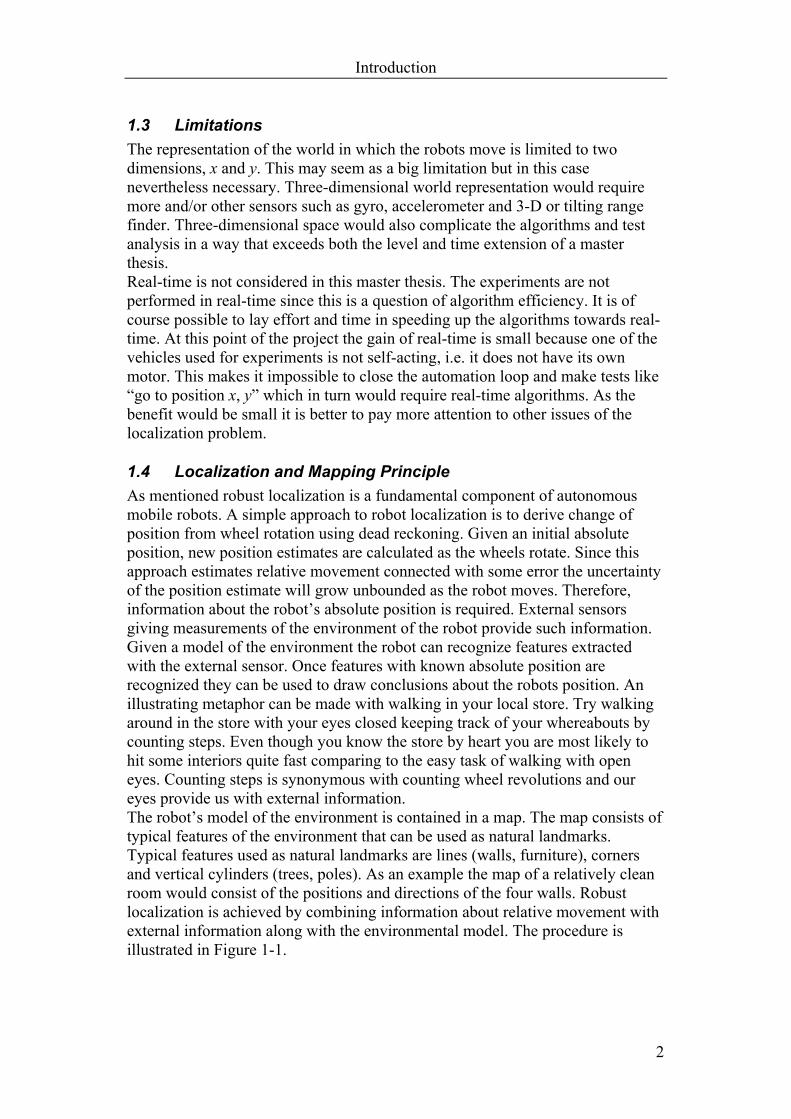
In the absence of Bilz2 an assisting sensor platform was constructed in form of a wagon with the necessary sensors and computer mounted. This assisting platform will in the report be referred to as “the vehicle”. The second sensor platform is a commercial research robot from ActivMedia Robotics called Pioneer 2 [16].
2.1 The vehicle The vehicle consists of a 4-wheel wagon carrying a computer and sensors in form of a range finder and two separate wheel encoders. The vehicle is steered with the front wheels while the rear wheels are passive, independent and free rolling. The wheels have rubber tires giving good friction and quite low slippage at moderate speeds. As the rear tires have the properties described above they are well suited for relative positioning by use of encoders. The vehicle has no motors but is moved by hand of an operator. A picture of the vehicle is seen in Figure 2-2.
Sensor Platforms
7
Figure 2-2
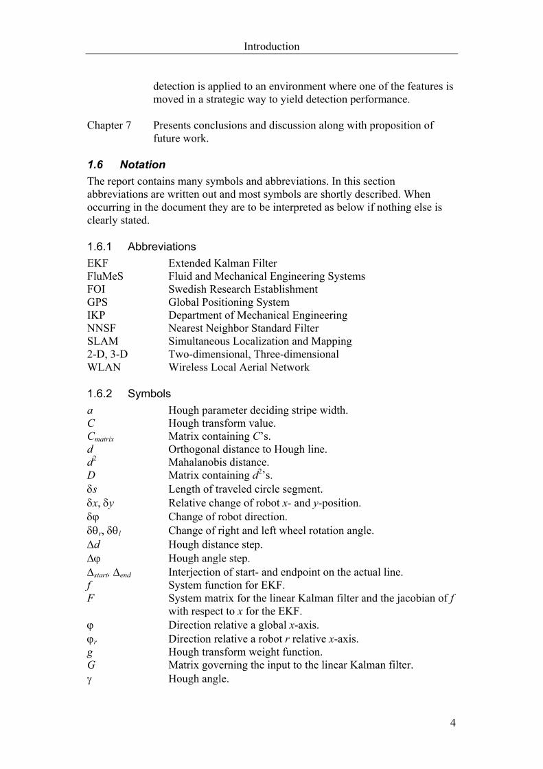
2.2 Pioneer 2 The other sensor platform is as mentioned previously the Pioneer 2 from ActivMedia Robotics. It is a commercial research robot delivered with ready to use hardware and software. The Pioneer is equipped with the same range finder as the vehicle along with individual encoders. Additionally, it is also equipped with sonars, which are very useful if one wishes to avoid collisions. The laser range finder can of course also be used for collision avoidance but has the drawback that it does not always detect windows and mirrors. The Pioneer has three wheels, two front wheels and one rear. Controlling individual motors for each front wheel moves the robot while the rear wheel simply acts as a slave for balance.
Figure 2-3 The Pioneer 2.
Sensor Platforms
8
2.3 Sensors
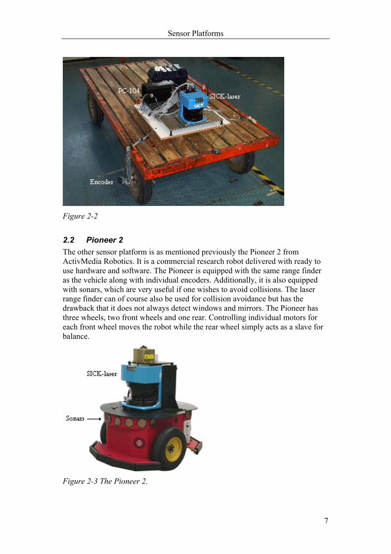
2.3.1 Encoders The encoders are optical encoders series 5540 manufactured by Faulhaber. The high-resolution encoders can detect the angular displacement, speed and direction of rotation. The maximum resolution in angular displacement is 360°/2000 equaling 0.18°. Each encoder have three outputs channels A, B and I showed in Figure 2-4.
Figure 2-4 The output channels from the encoder.
Channel I goes high one time per revolution thus enabling easy track of the number of full revolutions. Channels A and B are phase shifted 90° and give 500 pulses per revolution each. The direction of rotation is decided by the order in which positive flanks appear for channel A and B. The time between two positive flanks is the time it takes for an angular change of 360°/500 = 0.72° and hence inversely proportional to angular speed. By choosing to count on positive and negative flank on both channels the maximum angular resolution is reached.
2.3.2 Range Finder The range finder is a time of flight laser giving the distance to the first reflecting object in the environment of the sensor. The operating principle is to launch beams with limited extension and detect the time from launch to return.
Sensor Platforms
9
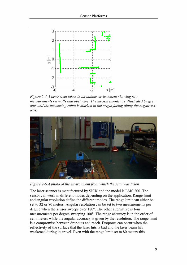
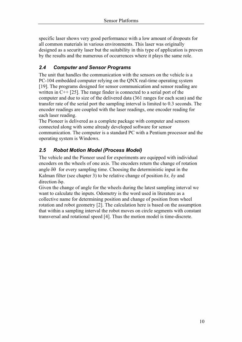
Figure 2-5 A laser scan taken in an indoor environment showing raw measurements on walls and obstacles. The measurements are illustrated by grey dots and the measuring robot is marked in the origin facing along the negative x-axis.
Figure 2-6 A photo of the environment from which the scan was taken.
The laser scanner is manufactured by SICK and the model is LMS 200. The sensor can work in different modes depending on the application. Range limit and angular resolution define the different modes. The range limit can either be set to 32 or 80 meters. Angular resolution can be set to two measurements per degree when the sensor sweeps over 180°. The other alternative is four measurements per degree sweeping 100°. The range accuracy is in the order of centimeters while the angular accuracy is given by the resolution. The range limit is a compromise between dropouts and reach. Dropouts can occur when the reflectivity of the surface that the laser hits is bad and the laser beam has weakened during its travel. Even with the range limit set to 80 meters this
Sensor Platforms
10
specific laser shows very good performance with a low amount of dropouts for all common materials in various environments. This laser was originally designed as a security laser but the suitability in this type of application is proven by the results and the numerous of occurrences where it plays the same role.
2.4 Computer and Sensor Programs The unit that handles the communication with the sensors on the vehicle is a PC-104 embedded computer relying on the QNX real-time operating system [19]. The programs designed for sensor communication and sensor reading are written in C++ [25]. The range finder is connected to a serial port of the computer and due to size of the delivered data (361 ranges for each scan) and the transfer rate of the serial port the sampling interval is limited to 0.3 seconds. The encoder readings are coupled with the laser readings, one encoder reading for each laser reading. The Pioneer is delivered as a complete package with computer and sensors connected along with some already developed software for sensor communication. The computer is a standard PC with a Pentium processor and the operating system is Windows.
2.5 Robot Motion Model (Process Model) The vehicle and the Pioneer used for experiments are equipped with individual encoders on the wheels of one axis. The encoders return the change of rotation angle δθ for every sampling time. Choosing the deterministic input in the Kalman filter (see chapter 3) to be relative change of position δx, δy and direction δϕ. Given the change of angle for the wheels during the latest sampling interval we want to calculate the inputs. Odometry is the word used in literature as a collective name for determining position and change of position from wheel rotation and robot geometry [2]. The calculation here is based on the assumption that within a sampling interval the robot moves on circle segments with constant transversal and rotational speed [4]. Thus the motion model is time-discrete.

Sensor Platforms
11
Figure 2-7 The axis equipped with encoders at two subsequent time points t = k-1 and t = k. Now defining variables needed for the calculation. According to Figure 2-7: δϕ The change of the robot’s direction.
rs , δs, sl Length of traveled circle segment for right wheel, centre of axis, left wheel.
Ld/2 Half of the diagonal distance between centre of axis at the subsequent time points.
rl, rr Left and right wheel radius. La Distance between left and right wheel (length of wheel
axis). Lrc, Lrl, Lrr Radius from centre of rotation to: center of axis, left
wheel, and right wheel. δθl , δθr Change of angle for left and right wheel between times
between two sampling times.
Table 2.1 Variables used for calculation of inputs δx, δy and δϕ. Some elemental relations give
δϕδθ rllll Lrs == (2.1) δϕδθ rrrrr Lrs == (2.2)
δϕδ rcLs = (2.3)
rrrla LLL −= (2.4)
2rlrr
rcLL
L+
= . (2.5)
Equation (2.1), (2.2) and (2.4) give
Sensor Platforms
12
( )rrlla
rrL
δθδθδϕ −=1 , (2.6)
and (2.1)-(2.3) with (2.5) yield
( ) ( )rrllrrrl rrLLs δθδθδϕδϕδ +=+=21
21 . (2.7)
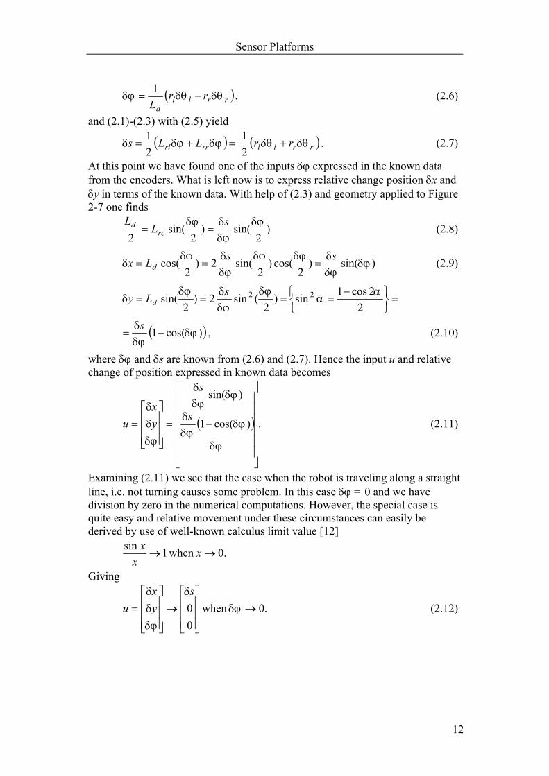
At this point we have found one of the inputs δϕ expressed in the known data from the encoders. What is left now is to express relative change position δx and δy in terms of the known data. With help of (2.3) and geometry applied to Figure 2-7 one finds
)2
sin()2
sin(2
δϕδϕδδϕ sL
Lrc
d == (2.8)
)sin()2
cos()2
sin(2)2
cos( δϕδϕδδϕδϕ
δϕδδϕ
δssLx d === (2.9)
=
−
====2
2cos1sin)2
(sin2)2
sin( 22 αα
δϕδϕδδϕ
δsLy d
( ))cos(1 δϕδϕδ
−=s , (2.10)
where δϕ and δs are known from (2.6) and (2.7). Hence the input u and relative change of position expressed in known data becomes
( ) .)cos(1
)sin(
−=
=
δϕ
δϕδϕδ
δϕδϕδ
δϕδδ
s
s
yx
u (2.11)
Examining (2.11) we see that the case when the robot is traveling along a straight line, i.e. not turning causes some problem. In this case δϕ = 0 and we have division by zero in the numerical computations. However, the special case is quite easy and relative movement under these circumstances can easily be derived by use of well-known calculus limit value [12]
1sin→
xx when .0→x
Giving
0. when 00 →
→
= δϕ
δ
δϕδδ syx
u (2.12)
Kalman Filter Theory and Data Association
13
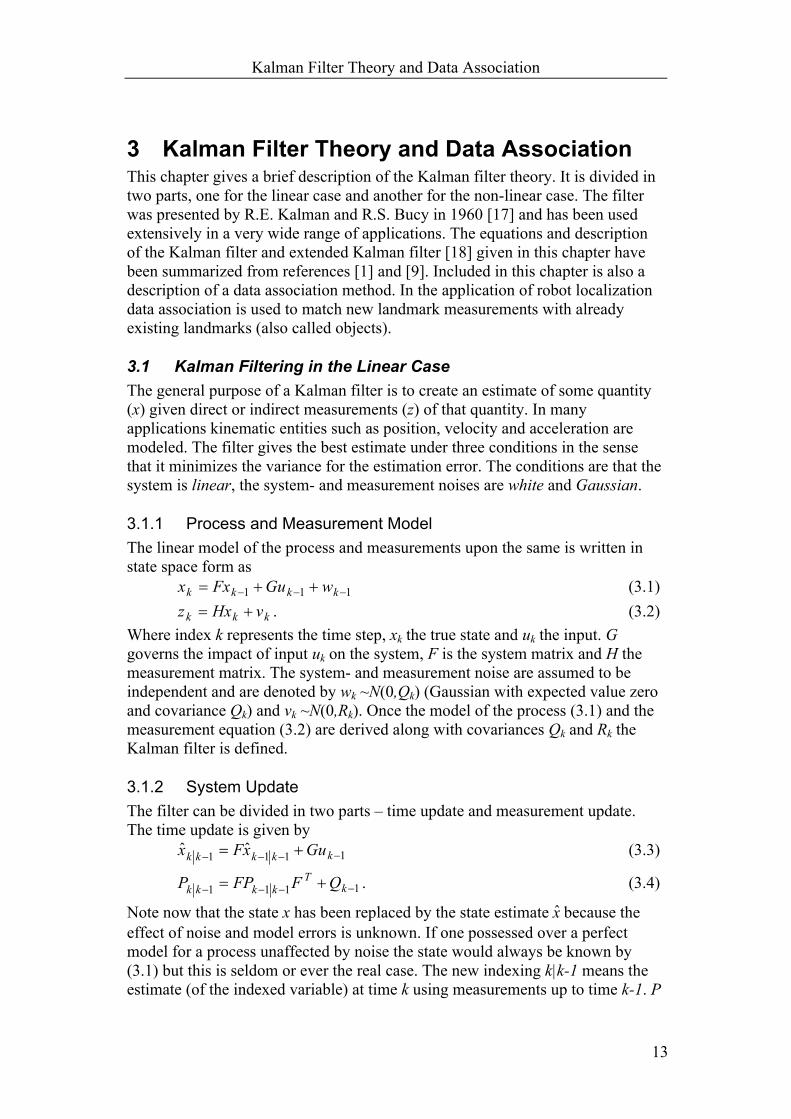
3 Kalman Filter Theory and Data Association This chapter gives a brief description of the Kalman filter theory. It is divided in two parts, one for the linear case and another for the non-linear case. The filter was presented by R.E. Kalman and R.S. Bucy in 1960 [17] and has been used extensively in a very wide range of applications. The equations and description of the Kalman filter and extended Kalman filter [18] given in this chapter have been summarized from references [1] and [9]. Included in this chapter is also a description of a data association method. In the application of robot localization data association is used to match new landmark measurements with already existing landmarks (also called objects).
3.1 Kalman Filtering in the Linear Case The general purpose of a Kalman filter is to create an estimate of some quantity (x) given direct or indirect measurements (z) of that quantity. In many applications kinematic entities such as position, velocity and acceleration are modeled. The filter gives the best estimate under three conditions in the sense that it minimizes the variance for the estimation error. The conditions are that the system is linear, the system- and measurement noises are white and Gaussian.
3.1.1 Process and Measurement Model The linear model of the process and measurements upon the same is written in state space form as
111 −−− ++= kkkk wGuFxx (3.1)
kkk vHxz += . (3.2) Where index k represents the time step, xk the true state and uk the input. G governs the impact of input uk on the system, F is the system matrix and H the measurement matrix. The system- and measurement noise are assumed to be independent and are denoted by wk ~N(0,Qk) (Gaussian with expected value zero and covariance Qk) and vk ~N(0,Rk). Once the model of the process (3.1) and the measurement equation (3.2) are derived along with covariances Qk and Rk the Kalman filter is defined.
3.1.2 System Update The filter can be divided in two parts – time update and measurement update. The time update is given by
1111 ˆˆ −−−− += kkkkk GuxFx (3.3)
1111 −−−− += kT
kkkk QFFPP . (3.4)
Note now that the state x has been replaced by the state estimate x because the effect of noise and model errors is unknown. If one possessed over a perfect model for a process unaffected by noise the state would always be known by (3.1) but this is seldom or ever the real case. The new indexing k|k-1 means the estimate (of the indexed variable) at time k using measurements up to time k-1. P
Kalman Filter Theory and Data Association
14
is the state estimate variance. Equation (3.3) is simply the known part of (3.1), i.e. everything except the noise. The first part of (3.4) is the old state estimate variance turned to the new state. The second part is the added uncertainty due to unknown noise and model error.
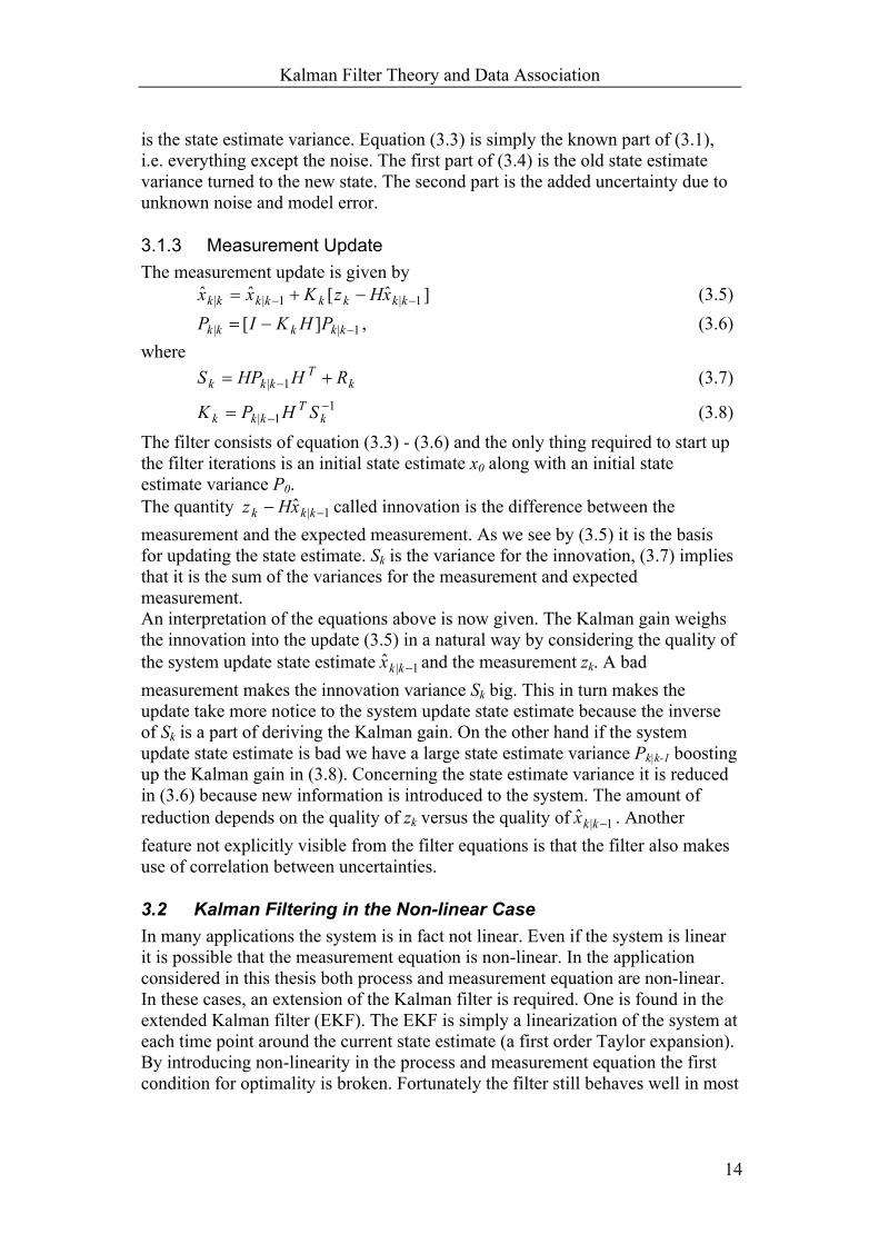
3.1.3 Measurement Update The measurement update is given by
]ˆ[ˆˆ 1|1|| −− −+= kkkkkkkk xHzKxx (3.5)
1|| ][ −−= kkkkk PHKIP , (3.6) where
kT
kkk RHHPS += −1| (3.7) 1
1|−
−= kT
kkk SHPK (3.8) The filter consists of equation (3.3) - (3.6) and the only thing required to start up the filter iterations is an initial state estimate x0 along with an initial state estimate variance P0. The quantity 1|ˆ −− kkk xHz called innovation is the difference between the measurement and the expected measurement. As we see by (3.5) it is the basis for updating the state estimate. Sk is the variance for the innovation, (3.7) implies that it is the sum of the variances for the measurement and expected measurement. An interpretation of the equations above is now given. The Kalman gain weighs the innovation into the update (3.5) in a natural way by considering the quality of the system update state estimate 1|ˆ −kkx and the measurement zk. A bad measurement makes the innovation variance Sk big. This in turn makes the update take more notice to the system update state estimate because the inverse of Sk is a part of deriving the Kalman gain. On the other hand if the system update state estimate is bad we have a large state estimate variance Pk|k-1 boosting up the Kalman gain in (3.8). Concerning the state estimate variance it is reduced in (3.6) because new information is introduced to the system. The amount of reduction depends on the quality of zk versus the quality of 1|ˆ −kkx . Another feature not explicitly visible from the filter equations is that the filter also makes use of correlation between uncertainties.
3.2 Kalman Filtering in the Non-linear Case In many applications the system is in fact not linear. Even if the system is linear it is possible that the measurement equation is non-linear. In the application considered in this thesis both process and measurement equation are non-linear. In these cases, an extension of the Kalman filter is required. One is found in the extended Kalman filter (EKF). The EKF is simply a linearization of the system at each time point around the current state estimate (a first order Taylor expansion). By introducing non-linearity in the process and measurement equation the first condition for optimality is broken. Fortunately the filter still behaves well in most
Kalman Filter Theory and Data Association
15
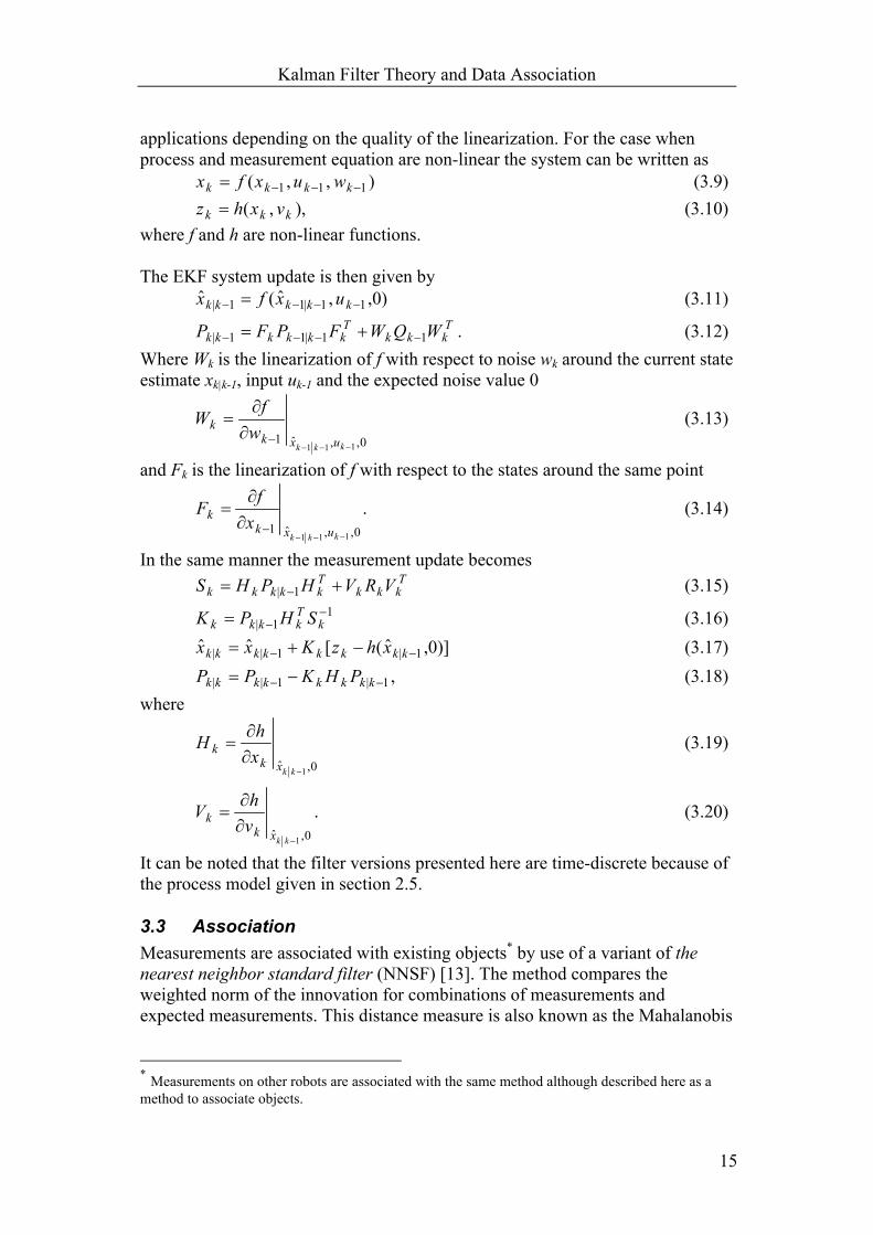
applications depending on the quality of the linearization. For the case when process and measurement equation are non-linear the system can be written as
),,( 111 −−−= kkkk wuxfx (3.9) ),,( kkk vxhz = (3.10)
where f and h are non-linear functions. The EKF system update is then given by
)0,,ˆ(ˆ 11|11| −−−− = kkkkk uxfx (3.11) Tkkk
Tkkkkkk WQWFPFP 11|11| −−−− += . (3.12)
Where Wk is the linearization of f with respect to noise wk around the current state estimate xk|k-1, input uk-1 and the expected noise value 0
0,,ˆ1111 −−−
−∂∂
=kkk uxk
k wfW (3.13)
and Fk is the linearization of f with respect to the states around the same point
.0,,ˆ1
111 −−−−∂
∂=
kkk uxkk x
fF (3.14)
In the same manner the measurement update becomes Tkkk
Tkkkkk VRVHPHS += −1| (3.15)
11|
−−= k
Tkkkk SHPK (3.16)
)]0,ˆ([ˆˆ 1|1|| −− −+= kkkkkkkk xhzKxx (3.17) ,1|1|| −− −= kkkkkkkk PHKPP (3.18)
where
0,ˆ 1−∂∂
=kkxk
k xhH (3.19)
0,ˆ 1−∂∂
=kkxk
k vhV . (3.20)
It can be noted that the filter versions presented here are time-discrete because of the process model given in section 2.5.
3.3 Association Measurements are associated with existing objects* by use of a variant of the nearest neighbor standard filter (NNSF) [13]. The method compares the weighted norm of the innovation for combinations of measurements and expected measurements. This distance measure is also known as the Mahalanobis
* Measurements on other robots are associated with the same method although described here as a method to associate objects.

Kalman Filter Theory and Data Association
16
distance. Denoting measurement i with )(iz and the expected measurement on object j with )(ˆ jz . The weighted norm for )(iz and )(ˆ jz is then given by
[ ] [ ])()(1)()(2, ˆˆ jiTjiji zzSzzd −−= − , (3.21)
where S is the variance of the innovation given in (3.15). In a situation where m existing objects are to be compared with n extracted measurements the distances of all possible combinations are given by the elements in
.),(2
,2,1
21,
21,1
=
nmn
m
dd
ddmnD (3.22)
When D has been computed, associations between measurements and objects are to be made. In the original algorithm minimizing the sum of all combinations of measurements and objects reveals the associations under the assumption that only one measurement can belong to one object. Expressed as an optimization problem this is solved by following two cases. Case 1, mn ≤ :
∑∑= =
n
i
m
jjiji dx
1 1
2,,min
when
∑=
∀=m
jji ix
1, ,1
{ }1 ,0, ∈jix (binary) Case 2, mn > :
∑∑= =
m
j
n
ijiji dx
1 1
2,,min
when
∑=
∀=n
iji jx
1, ,1
{ }1 ,0, ∈jix (binary) Note that x in the problem above is not a state but merely a help variable used in the optimization problem. The complexity and computation burden is quite heavy especially as the number of objects and measurements increase. However, if an initial gating is used, i.e. only those combinations with sufficiently small 2
, jid are considered, this is drastically reduced. Here we use an even simpler and faster approach by associating measurements with objects one at a time. The first step is to sort out the objects not local to the position where the measurement was conducted. Since the robots may have traversed large distances and the reach of the range finder is limited there is no point in comparing with all

Kalman Filter Theory and Data Association
17
existing objects. Additionally only objects and extracted measurements with small Euclidean separation are compared. The following comparison sees to that
( ) ,)ˆ()ˆ( max212)()(2)()( rzzzz j
yi
yj
xi
x <−+− (3.23) where lowered indexes stand for x- and y-position. If the condition above is fulfilled the angle difference between the measurement and expected measurement is checked. Depending on which direction angles are decided a correction may be required. As an example if the angle is counted clockwise for the measurement and counter clockwise for the correct expected measurement they will be faulty separated by about π. This is detected by checking if the angular difference is larger than π/2. In this case the angle of the expected measurement is corrected by
])(
[)(
ππ ϕϕ
ϕϕ
ojzzzz
−−= (3.24)
where the brackets indicate a function that returns the closest integer and lowered index stands for direction. After this preprocessing D in (3.22) is computed for the measurements and the objects that have fulfilled the conditions above. Associations are then made by picking the smallest value one by one in D followed by elimination of corresponding row and column in D for each pick. Sometimes objects that do not exist in the filter are extracted from measurements. Therefore, all extracted objects should not always be associated with existing objects. To govern this a threshold on the Mahalanobis distance is set for deciding whether an object and measurement should be associated. If object j and measurement i currently has the smallest distance in D they should be associated if the following condition is fullfilled
.2max
2, dd ji ≤ (3.25)
Under the condition that correct associations always are made the Mahalanobis distance is χ2 distributed. By studying a χ2 distribution table a hint is given to the size of the threshold value. Given that the variances of the measurements and expected measurements are correct the right associations are made with some probability given by the threshold and the distribution table. The described variant of NNSF is easier and computationally more efficient then the original algorithm. One drawback is however identified as the risk for faulty associations. A situation where faulty associations would occur when applying the variant is illustrated in Figure 3-1.
Kalman Filter Theory and Data Association
18
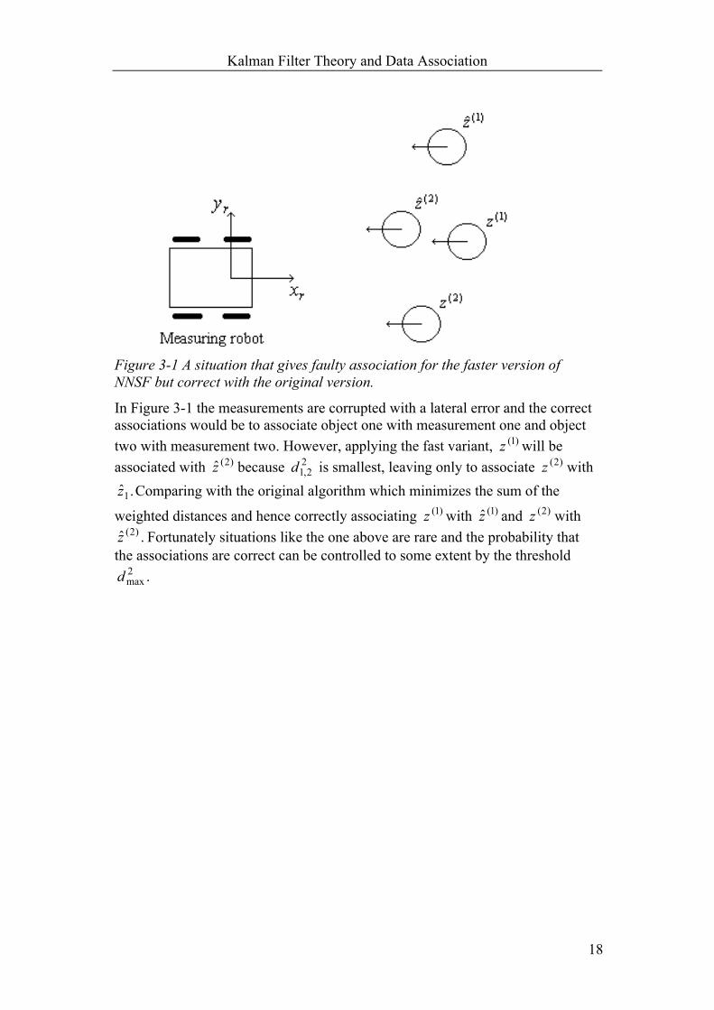
Figure 3-1 A situation that gives faulty association for the faster version of NNSF but correct with the original version.
In Figure 3-1 the measurements are corrupted with a lateral error and the correct associations would be to associate object one with measurement one and object two with measurement two. However, applying the fast variant, )1(z will be associated with )2(z because 2
2,1d is smallest, leaving only to associate )2(z with .ˆ1z Comparing with the original algorithm which minimizes the sum of the
weighted distances and hence correctly associating )1(z with )1(z and )2(z with .ˆ )2(z Fortunately situations like the one above are rare and the probability that
the associations are correct can be controlled to some extent by the threshold .2
maxd
Localization and Mapping
19
4 Localization and Mapping A prerequisite for a robot to work autonomously is that it possesses a reliable estimate of its own global position. Global localization requires exteroceptive sensors providing information of the environment. In our case the laser range finder provides us with landmarks (also called objects) and information about them. By letting several robots cooperate and exchange information more accurate localization can be reached. The centralized Kalman filter described in this chapter is one approach to handle several robots and objects in an organized way.
4.1 The Simulated Filter As mentioned in the introduction to the thesis a centralized Kalman filter used in simulations was used as a take off. Positions of robots and objects are represented as states in the filter. Each position consists of three states xx, xy and xϕ representing global x, y position and direction. Direction xϕ is defined as the angle between the global x-axis and the heading of the robot or object. Objects may or may not have direction depending on the physical nature of the real object that is modeled. As an example a vertical cylinder does not have direction in contrary to a wall which does. However, for completeness all objects are given an angle although not used for objects such as the vertical cylinder. The simulation program consists of m robots and n objects making the state x take the form
Tonony
onx
ojojy
ojx
ooy
ox
rmrmy
rmx
ririy
rix
rry
rx
xxxxxxxxx
xxxxxxxxxx
),,,,,,,,,
,,,,,,,,,,,()()()()()()()1()1()1(
)()()()()()()1()1()1(
ϕϕϕ
ϕϕϕ=
where raised index ri denotes robot number i and oj object number j. There is a distinct difference between robots and objects. Objects are fix while robots are mobile and possess a motion model. The motion and motion model of the robots are controlled by the input u. Given this background the process (equation (3.9)) takes the form
,),,(
),,(
)(1
)1(1
)(1
)(1
)(1
)(
)1(1
)1(1
)1(1
)1(
)(
)1(
)(
)1(
=
−
−
−−−
−−−
onk
ok
rmk
rmk
rmk
rm
rk
rk
rk
r
onk
ok
rmk
rk
x
xwuxf
wuxf
x
xx
x
(4.1)
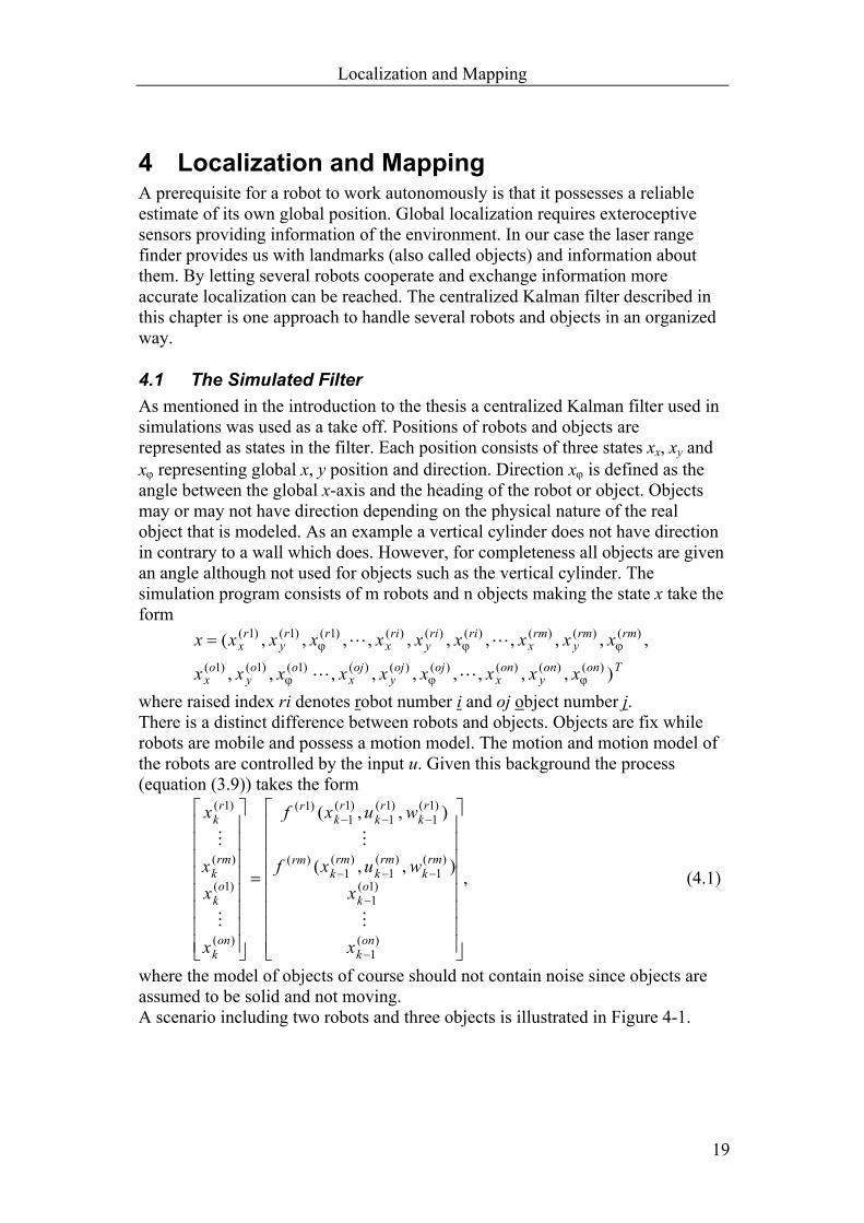
where the model of objects of course should not contain noise since objects are assumed to be solid and not moving. A scenario including two robots and three objects is illustrated in Figure 4-1.

Localization and Mapping
20
Figure 4-1 Two robots and three objects in the global coordinate system xg, yg.
The filter performs sequential measurement update. If one robot delivers measurements upon several objects at one sampling time the measurement update is performed one at a time for each object measurement. If the simulations are to imitate reality it is a fact that the range finder is onboard the moving robot and thus delivering measurements in coordinates relative to the measuring robot. This means that h in measurement equation (3.10) is a transformation from global to robot relative coordinates of the measuring robot because all states are given in global coordinates. The transformation is also the reason for why the process is non-linear. The measurement equation is unique for each pair of measuring robot and measured object. If robot number i measures object j (3.10) is written
),(),,( ),()()()( vxhzzz ojriTojojy
ojx =ϕ . (4.2)
As a consequence of the uniqueness of h the linearization (3.19) is recalculated for each sequential measurement update of one sampling time. A flow chart showing the general execution of the simulation program is viewed in Figure 4-2.
Localization and Mapping
21
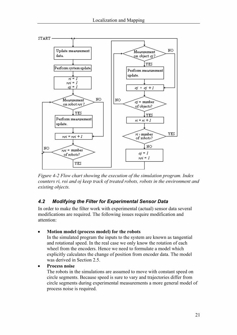
Figure 4-2 Flow chart showing the execution of the simulation program. Index counters ri, roi and oj keep track of treated robots, robots in the environment and existing objects.
4.2 Modifying the Filter for Experimental Sensor Data In order to make the filter work with experimental (actual) sensor data several modifications are required. The following issues require modification and attention: • Motion model (process model) for the robots
In the simulated program the inputs to the system are known as tangential and rotational speed. In the real case we only know the rotation of each wheel from the encoders. Hence we need to formulate a model which explicitly calculates the change of position from encoder data. The model was derived in Section 2.5.
• Process noise The robots in the simulations are assumed to move with constant speed on circle segments. Because speed is sure to vary and trajectories differ from circle segments during experimental measurements a more general model of process noise is required.

Localization and Mapping
22
• Measurement equation
The simulated measurements where initially given in global coordinates. As mentioned above this is not the real case because the range finder is mounted on the moving robot.
• Extract objects and robots from laser data In the simulation program robots try to measure upon all existing objects and other robots. Under certain circumstances (no occlusion and correct direction) these measurements are delivered. For experimental measurements, objects are extracted from raw range data.
• Associate objects and robots The extracted objects have to be associated with existing objects. Without association there is no expected measurement to compare with. Association was described in Section 3.3.
• Add new objects Extracted objects that are not associated with existing may be useful as new landmarks. Therefore, the filter needs to be dynamic in the sense that new objects can be added. The unassociated objects are added under certain criterions such as length and variance.
• Combine measurements from different time points originating from robots with different sampling interval The simulation program assumes that measurements from different robots arrive at the same time with the same sampling interval. Experimental measurements do not fulfill this assumption. We have a situation where the robots are not homogenous, even the hardware is different on the two robots.
A flow chart showing the general execution of the modified filter is viewed in Figure 4-3.
Localization and Mapping
23
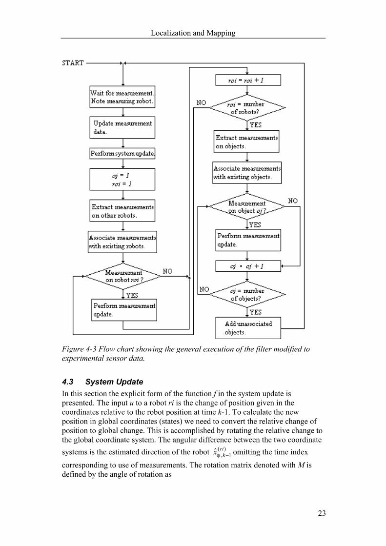
Figure 4-3 Flow chart showing the general execution of the filter modified to experimental sensor data.
4.3 System Update In this section the explicit form of the function f in the system update is presented. The input u to a robot ri is the change of position given in the coordinates relative to the robot position at time k-1. To calculate the new position in global coordinates (states) we need to convert the relative change of position to global change. This is accomplished by rotating the relative change to the global coordinate system. The angular difference between the two coordinate systems is the estimated direction of the robot )(
1,ˆ rikx −ϕ omitting the time index
corresponding to use of measurements. The rotation matrix denoted with M is defined by the angle of rotation as
Localization and Mapping
24
( ) ( )( ) ( ) .
1000ˆcosˆsin
0ˆsinˆcos
)ˆ( )(1,
)(1,
)(1,
)(1,
)(1,
−
= −−
−−
−rik
rik
rik
rik
rik xx
xxxM ϕϕ
ϕϕ
ϕ (4.3)
The system update for robot ri with the notation of equation (4.1) becomes =+== −−−−− 1
)(1,
)(111
)()( )ˆ(ˆ)0,,ˆ(ˆ krik
rikkk
ririk uxMxuxfx ϕ
( ) ( )( ) ( ) .
1000ˆcosˆsin
0ˆsinˆcos
ˆ
ˆ
ˆ
)(1
)(1
)(1
)(1,
)(1,
)(1,
)(1,
)(1,
)(1,
)(1,
−
+
=
−
−
−
−−
−−
−
−
−
rik
rik
rik
rik
rik
rik
rik
rik
riky
rikx
yx
xxxx
xxx
δϕδδ
ϕϕ
ϕϕ
ϕ
(4.4)
As mentioned earlier the measurement update is performed sequentially which means that the same applies to the system update. As a consequence when the treated robot is ri the system update (3.11) becomes
,ˆ
)0,,ˆ(
ˆ
)0,,ˆ(ˆ)1(
1
)(1
)(1
)(
)1(1
11
==
−
−−
−
−−o
k
rik
rik
ri
rk
kkk
xuxf
x
uxfx (4.5)
where )0,,ˆ( )(1
)(1
)( rik
rik
ri uxf −− is given by (4.4). Now linearizing f with respect to the states to obtain Fk in (3.12)
,
1000
10
010
001
0,,ˆ)(1
)(
0,,ˆ1111111
∂
∂=
∂∂
=−−−−−−
−−kkkkkk ux
rik
ri
uxkk x
f
xfF (4.6)
where
=
∂
∂
∂
∂
∂
∂
∂
∂
∂
∂
∂
∂
∂
∂
∂
∂
∂
∂
=
==∂
∂
−−−
−−−−
0,,ˆ)(
)(
)(
)(
)(
)(
)(
)(
)(
)(
)(
)(
)(
)(
)(
)(
)(
)(
0,,ˆ)(1
)(
111
111
kkk
kkk
uxri
ri
riy
ri
rix
ri
ri
riy
riy
riy
rix
riy
ri
rix
riy
rix
rix
rix
y
x
uxri
k
ri
x
f
x
f
x
fx
f
x
f
x
fxf
xf
xf
fff
fxf
ϕ
ϕϕϕ
ϕ
ϕ
ϕ
Localization and Mapping
25
( ) ( )( ) ( ) .xyxx
xyxxrik
rik
rik
rik
rik
rik
rik
rik
−
−−
= −−−−
−−−−
100ˆsinˆcos10
ˆcosˆsin01)(
1,)(1
)(1,
)(1
)(1,
)(1
)(1,
)(1
ϕϕ
ϕϕ
δ
δδ
(4.7)
By (4.5)-(4.7) the system update is known except for the last part of (3.12) which is derived in the following section.
4.4 Process Noise When calculating the inputs δx, δy and δϕ from the change of angle for each tire and geometry it is certain that errors occur. The main sources of error are the odometric parameters [2]: effective wheel radius (rr, rl), effective axis length (La) and resolution of encoders. Another source of error is the chosen model, i.e. model error. The model holds under two assumptions: • The robots move with constant speed on circle segments within each
sampling interval. • The tires of the robots do not slip. Both assumptions are bound to be broken to some extent. The trajectory of a robot may deviate from a circle segment due to change of speed or even direction during a sampling interval. Limited friction between the tires and contact surface cause robots to slip while accelerating, braking and turning. The sum of errors can be interpreted as the system noise w. The system noise can be decomposed into two parts each depending on the origin. The two parts are noise due to model error wm and noise due to uncertainties in odometric parameters wp.
pm www +=
(4.8) Letting ut denote the true input or true relative change of position we have
,wuut += (4.9) where
[ ] .Tyxu δϕδδ=
4.4.1 Noise from Odometric Parameters Noise originating from the odometric parameters is collected in wp. After calibration of rl, rr and La, which eliminates the systematic errors [2], we are left with non-systematic errors. Repeating the sources of error: effective wheel radius (rr, rl), effective axis length (La) and resolution of encoder. A more detailed description of the first two is motivated. Effective wheel radius changes due to uneven contact surface and travel over unexpected objects such as gravel. Effective axis length changes due to tire deformations and uneven contact surface. By viewing equation (2.6), (2.7), (2.11) and (2.12) it is obvious that the covariance matrix for wp will contain correlation terms. In order to calculate the covariance matrix for wp we write the corresponding input as a function of the odometric parameters.
Localization and Mapping
26
==
)()()(
)(
3
2
1
OqOqOq
Oqyx
δϕδδ
(4.10)
where O are the odometric variables [ ]Tarl LO δθδθrl rr= .
Equation (2.6), (2.7) and (2.11) give ( )
( ) ( )
−
−+
= rrllarrll
rrlla rrLrr
rrLOq δθδθ
δθδθδθδθ 1sin
2)(1
( )( ) ( )
−−
−+
= rrllarrll
rrlla rrLrr
rrLOq δθδθ
δθδθδθδθ 1cos1
2)(2
( )rrlla
rrL
Oq δθδθ −=1)(3
and equation (2.6), (2.7) and (2.12) for the case of straight line movement
( )rrll rrOq δθδθ +=21)(1
0)(2 =Oq .0)(3 =Oq
It is possible to make good estimations of the variance for all variables in O. Assuming that the variances for the variables in O are not correlated, Var(O) will be diagonal (5×5) matrix with the variance for each variable along the diagonal. Denoting the variance for each variable with 22 , δθσσ r and 2
aLσ . The variance for effective wheel radius and change of angle are the same for left and right wheel why no left and right indices are needed. Now using straightforward error analysis [3] for q in equation (4.10). A first order Taylor expansion around the expected value O0 of the odometric variables gives
),()( 00 OOOqOqq −
∂∂
+≈ (4.11)
where
∂∂
∂∂
∂∂
∂∂
∂∂
∂∂
∂∂
∂∂
∂∂
=∂∂
arl
arl
arl
Lq
rq
rq
Lq
rq
rq
Lq
rq
rq
Oq
333
222
111
. (4.12)
Which in turn yields
Localization and Mapping
27
( ) ( ) =∂∂
−∂∂
≈−==T
p OqOOE
OqOqqEqVarwVar 2
02
0 )()()(
.)(T
OqOVar
Oq
∂∂
∂∂
= (4.13)
This approximation is known as “Gauss approximation formula”. The elements in (4.12) are calculated by using a symbol treating mathematics program such as Maple.
4.4.2 Model Error The no slip and circle segment travel assumptions lead to deviations from the true change of relative position when calculating u. It is reasonable that these deviations grow as relative change of position grows. A first approach is to let the covariance matrix for wm be a diagonal matrix with elements proportional to the length of the traveled arc δs.
,00
0000
)(
,
=sk
sksk
wVar
s
y
x
m
δδ
δ
δϕ
where kx, ky and kϕ,δs are constant design parameters. But then we imply that the robot can rotate around its own axis without ever losing track of its own direction. It is also plausible that rotation during travel affects the errors in x, y position because such movement introduces sideslip. In other words rotation of course effects uncertainty in direction as well as uncertainty in x, y position. Hence the covariance matrix is extended as
,00
0000
)(
,
,
,
++
+=
δϕδδϕδ
δϕδ
ϕδϕ
ϕ
ϕ
kskksk
kskwVar
s
yy
xx
m (4.14)
where kx, ky, kϕ,δs, kx,ϕ, ky,ϕ and kϕ are constant design parameters. Equation (4.13) and (4.14) summarizes to the system noise covariance matrix Q
)()( mp wVarwVarQ += . (4.15) By (4.15) we are only left with the derivation of W in the system update (3.12). From (4.4) and (4.9) we realize that for updated robot ri the process model is
),)((),,( )(1
)(1
)(1,
)(1
)(1
)(1
)(1
)()( rik
rik
rik
rik
rik
rik
rik
ririk wuxMxwuxfx −−−−−−− ++== ϕ (4.16)
belonging to the process model for all robots and objects
Localization and Mapping
28
.),,(
),,(
),,(
)(1
)1(1
)(1
)(1
)(1
)(
)1(1
)1(1
)1(1
)1(
111
)(
)1(
)(
)1(
==
−
−
−−−
−−−
−−−
onk
ok
rmk
rmk
rmk
rm
rk
rk
rk
r
kkk
onk
ok
rmk
rk
x
xwuxf
wuxf
wuxf
x
xx
x
(4.17)
The linearization of f with respect to w becomes
,
)(1
)(
)(1
)1(
)2(1
)1(
)(1
)1(
)2(1
)1(
)1(1
)1(
1
∂
∂
∂
∂
∂
∂∂
∂
∂
∂
∂
∂
=∂
∂
−−
−
−−−
−
onk
on
onk
r
rk
r
onk
r
rk
r
rk
r
k
wf
wf
wf
wf
wf
wf
wf
where the only elements differing from zero are the ones corresponding to robots along the diagonal. The explicit calculation of such an element is easy, consider again robot ri then
( ) ).())(( )(1,
)(1
)(1
)(1,
)(1)(
1)(1
)(rik
rik
rik
rik
rikri
kri
k
rixMwuxMx
wwf
−−−−−−−
=++∂
∂=
∂
∂ϕϕ
This concludes the derivation of W by repeating (3.13)
0,,ˆ1111 −−−
−∂∂
=kkk uxk
k wfW .
4.5 Measurement Model The onboard laser sensor gives measurements on objects in the robot’s environment after extraction of objects from laser data. While the states for robots and objects are given in global coordinates, measurements are given in coordinates local to the robot as the laser is mounted on the robot. In order to express the measurement equation in terms of states a transformation from global to local coordinates is required. Consider Figure 4-4 illustrating the relation between the expected measurement, the estimated states of the measuring robot and the estimated states of the measured object in the two coordinate systems.

Localization and Mapping
29
Figure 4-4 Illustration of expected measurement in both global and robot relative coordinates. The object here illustrated as a line segment.
Imagine now that at some time point k robot ri delivers a measurement on object oj as in Figure 4-4. The expected measurement )0,ˆ(ˆ 1| −= kkk xhz expressed in global coordinates is simply the difference between the estimated state of the object and the measuring robot. Since the expected measurement is to be expressed in coordinates relative to the measuring robot the rotation matrix is also applied with the argument 1|,ˆ −− kkxϕ . If the tedious indexing k|k-1 is replaced with k the expected measurement for robot ri on object oj becomes
=−−== − )ˆˆ)(ˆ()0,ˆ(ˆ )()()(,1|
rik
ojk
rikkkk xxxMxhz ϕ
( ) ( )( ) ( ) =
−
−
−
−=)(
,)(
,
)(,
)(,
)(,
)(,
)(,
)(,
)(,
)(,
ˆˆˆˆˆˆ
1000ˆcosˆsin0ˆsinˆcos
rik
ojk
riky
ojky
rikx
ojkx
rik
rik
rik
rik
xxxxxx
xxxx
ϕϕ
ϕϕ
ϕϕ
( ) ( )( ) ( ) .
ˆˆˆcos)ˆˆ(ˆsin)ˆˆ(
ˆsin)ˆˆ(ˆcos)ˆˆ(
)(,
)(,
)(,
)(,
)(,
)(,
)(,
)(,
)(,
)(,
)(,
)(,
)(,
)(,
−
−+−−
−+−
=rik
ojk
rik
riky
ojky
rik
rikx
ojkx
rik
riky
ojky
rik
rikx
ojkx
xxxxxxxx
xxxxxx
ϕϕ
ϕϕ
ϕϕ
(4.18)
Now linearizing h in order to provide the measurement update (3.15)-(3.18) with Hk. Repeating that the considered measurement is robot ri measuring object oj and highlighting it by giving h the raised index (ri, oj). With this in mind it is obvious that the linearization of h will contain submatrices (3×3) of zeros at

Localization and Mapping
30
positions representing objects and robots not involved in the considered measurement.
=∂
∂=
∂∂
=−− 0,ˆ
),(
0,ˆ,11 kkkk xk
ojri
xkk x
hxhH
=
∂∂
∂∂
∂∂
∂∂
∂∂
∂∂
=
− 0,ˆ)(
),(
)(
),(
)1(
),(
)(
),(
)(
),(
)1(
),(
,1kkxon
k
ojri
ojk
ojri
ok
ojri
rmk
ojri
rik
ojri
rk
ojri
xh
xh
xh
xh
xh
xh
,0000000,ˆ
)(
),(
)(
),(
,1−
∂
∂
∂
∂=
kkxoj
k
ojri
rik
ojri
xh
xh (4.19)
where ( ) ( )( ) ( ) =
−
−+−−
−+−
∂
∂=
∂
∂
)(,
)(,
)(,
)(,
)(,
)(,
)(,
)(,
)(,
)(,
)(,
)(,
)(,
)(,
)()(
),(cos)(sin)(sin)(cos)(
rik
ojk
rik
riky
ojky
rik
rikx
ojkx
rik
riky
ojky
rik
rikx
ojkx
rik
rik
ojri
xxxxxxxx
xxxxxx
xxh
ϕϕ
ϕϕ
ϕϕ
=
−−−−−−
−+−−−−
=100
)sin()()cos()()cos()sin()cos()()sin()()sin()cos(
)(,
)(,
)(,
)(,
)(,
)(,
)(,
)(,
)(,
)(,
)(,
)(,
)(,
)(,
)(,
)(,
rik
riky
ojky
rik
rikx
ojkx
rik
rik
rik
riky
ojky
rik
rikx
ojkx
rik
rik
xxxxxxxxxxxxxxxx
ϕϕϕϕ
ϕϕϕϕ
−−
−
−+−−=000
)(00)(00
)()( )(,
)(,
)(,
)(,
)(,
)(,
rikx
ojkx
riky
ojky
rik
rik xx
xxxMxM ϕϕ (4.20)
and ( ) ( )( ) ( ) =
−
−+−−
−+−
∂
∂=
∂
∂
)(,
)(,
)(,
)(,
)(,
)(,
)(,
)(,
)(,
)(,
)(,
)(,
)(,
)(,
)()(
),(cos)(sin)(sin)(cos)(
rik
ojk
rik
riky
ojky
rik
rikx
ojkx
rik
riky
ojky
rik
rikx
ojkx
ojk
ojk
ojri
xxxxxxxx
xxxxxx
xxh
ϕϕ
ϕϕ
ϕϕ
( ) ( )( ) ( ) ).(
1000cossin0sincos
)(,
)(,
)(,
)(,
)(,
rik
rik
rik
rik
rik
xMxxxx
ϕϕϕ
ϕϕ
−=
−= (4.21)
4.6 Adding Objects to the Kalman Filter In the case when objects are extracted from laser data and not associated with already existing objects it is either a new object or a corrupt measurement. A corrupt measurement should be disregarded while a new object is to be added into the Kalman filter. To detect corrupt measurements it is assumed that they are erroneous measurements on existing objects. The nature of the unassociated measurements is then decided by applying the Mahalanobis distance from the

Localization and Mapping
31
preceding section with a higher threshold. The threshold is set with margin higher than the threshold used for associating objects and therefore requiring that new objects are sufficiently separated from existing. Should despite this filtering some corrupt measurement sneak into the filter it can be treated by keeping track of association. A corrupt object in the filter is not likely to be associated with following measurements. It can therefore be deleted after a certain time has passed without associations. Now turning to the case of a new object. Due to the fact that a new object is extracted from measurements relative to the position of the measuring robot it will be correlated with the robot as well as other existing robots and objects. The correlation to the measuring robot is obvious, as the position of the new object is a function of the measuring robots global position and the measurement. The correlation to other existing robots and objects is more indirect but follows from the fact that robot positions have been decided partly by associations of measurements onto the existing objects. Thus we conclude that adding an object requires two operations [5]: I. Enter the new object into the state vector x. II. Expand the state estimate covariance matrix P with the uncertainty of
the new object and its correlation with other objects and robots. To illustrate the procedure we imagine a situation when the system consists of m robots and n objects and a new object is to be added.
→
+ )1(
)(
)1(
)(
)1(
)(
)1(
)(
)1(
object new add
on
on
o
rm
r
on
o
rm
r
xx
xx
x
x
xx
x
(4.22)
,
=
ABBPP
Told
exp (4.23)
where
[ ]nnnn
nnn
n
old pppB ,
pp
pppp
P ,12,11,1
,1,
1,2
,12,11,1
+++=
=
and 1,1 ++= nnpA .
Above pi,i is the 3×3 covariance matrix for the state estimate of robot/object number i and pi,j is the 3×3 covariance matrix between the estimations of

Localization and Mapping
32
object/robot i and object/robot j. In order to find explicit expressions for the new parts A and B in the expanded state estimate covariance matrix Pexp we need to calculate the new object as a function of the measurement z and the position (state) of the measuring robot x(ri). Solving for the state representing the new object in the measurement equation (4.18) we find
,)(),( )1()()(1)(1
+++ +== nririnri
n zxMxzxgx ϕ (4.24) for which x(ri) is the state of the measuring robot and z(n+1) the measurement on the new object. Note that g here is not the Hough weight function but a locally used help function expressing the new object in terms of robot position and measurement. Linearizing g with respect to the states x and the measurement z(on+1) we get
=
∂
∂
∂
∂
∂
∂
∂
∂
∂
∂=
∂∂
=)()1()()()1( omornrirx
xg
xg
xg
xg
xg
xgG ………
∂
∂= 0000
)(rixg
(4.25)
)1( +∂
∂=
onzz
gG (4.26)
According to [5] we now derive the new parts of Pexp by the following equations oldx PGB = (4.27)
,Tzz
Txoldx RGGGPGA += (4.28)
where R is the variance matrix for the measurement. By completing the calculations and identifying Gz as the rotation matrix from robot relative- to global coordinates we see that the second part in (4.28) is simply the variance matrix for the measurement transformed to the latter coordinate system. Moreover if the multiplication of matrices in the first part of (4.28) is carried out one finds this part to be the effect on uncertainty for the new object arising from uncertainty in the measuring robot. It is easily seen that uncertainty in global (x,y)-position and direction for the measuring robot is added to the uncertainty for the same states of the new object. Moreover, uncertainty in direction for the robot also contributes to uncertainty in (x,y)-position for the new object by a heaving effect.
4.7 Object Estimation The laser range finder delivers raw range data from the environment of the robot. From raw data we wish to extract natural landmarks to be used for localization. This section presents extraction of two types of landmarks: Hough lines and line segments.
4.7.1 Hough Lines In fairly clean indoor environments the Hough transform can be applied to extract walls with good result [21]. Walls are very useful when localizing robots in indoor environments because they contain much information.
Localization and Mapping
33
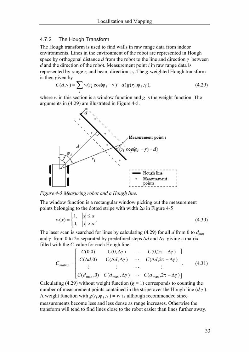
4.7.2 The Hough Transform The Hough transform is used to find walls in raw range data from indoor environments. Lines in the environment of the robot are represented in Hough space by orthogonal distance d from the robot to the line and direction γ between d and the direction of the robot. Measurement point i in raw range data is represented by range ri and beam direction ϕi. The g-weighted Hough transform is then given by
,),,())cos((),( ∑ −−=i
iiii rgdrwdC γϕγϕγ (4.29)
where w in this section is a window function and g is the weight function. The arguments in (4.29) are illustrated in Figure 4-5.
Figure 4-5 Measuring robot and a Hough line.
The window function is a rectangular window picking out the measurement points belonging to the dotted stripe with width 2a in Figure 4-5
>≤
=axax
xw,0,1
)( . (4.30)
The laser scan is searched for lines by calculating (4.29) for all d from 0 to dmax and γ from 0 to 2π separated by predefined steps ∆d and ∆γ giving a matrix filled with the C-value for each Hough line
.
)2,(),()0,(
)2,(),()0,()2,0(),0()0,0(
maxmaxmax
∆−∆
∆−∆∆∆∆∆−∆
=
γπγ
γπγγπγ
dCdCdC
dCdCdCCCC
Cmatrix (4.31)
Calculating (4.29) without weight function (g = 1) corresponds to counting the number of measurement points contained in the stripe over the Hough line (d,γ ). A weight function with iii rrg =),,( γϕ is although recommended since measurements become less and less dense as range increases. Otherwise the transform will tend to find lines close to the robot easier than lines further away.
Localization and Mapping
34
After calculating (4.31) the first line is found if the maximum C in Cmatrix exceeds a threshold. The procedure is then repeated after excluding the measurement points belonging to the recently found line. Extracted lines are finally improved by adapting them to their corresponding measurement points with the least square method.
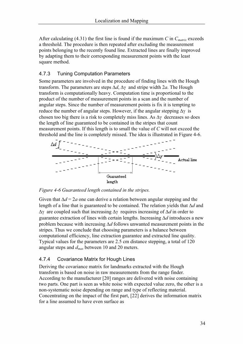
4.7.3 Tuning Computation Parameters Some parameters are involved in the procedure of finding lines with the Hough transform. The parameters are steps ∆d, ∆γ and stripe width 2a. The Hough transform is computationally heavy. Computation time is proportional to the product of the number of measurement points in a scan and the number of angular steps. Since the number of measurement points is fix it is tempting to reduce the number of angular steps. However, if the angular stepping ∆γ is chosen too big there is a risk to completely miss lines. As ∆γ decreases so does the length of line guaranteed to be contained in the stripes that count measurement points. If this length is to small the value of C will not exceed the threshold and the line is completely missed. The idea is illustrated in Figure 4-6.
Figure 4-6 Guaranteed length contained in the stripes.
Given that ∆d = 2a one can derive a relation between angular stepping and the length of a line that is guaranteed to be contained. The relation yields that ∆d and ∆γ are coupled such that increasing ∆γ requires increasing of ∆d in order to guarantee extraction of lines with certain lengths. Increasing ∆d introduces a new problem because with increasing ∆d follows unwanted measurement points in the stripes. Thus we conclude that choosing parameters is a balance between computational efficiency, line extraction guarantee and extracted line quality. Typical values for the parameters are 2.5 cm distance stepping, a total of 120 angular steps and dmax between 10 and 20 meters.
4.7.4 Covariance Matrix for Hough Lines Deriving the covariance matrix for landmarks extracted with the Hough transform is based on noise in raw measurements from the range finder. According to the manufacturer [20] ranges are delivered with noise containing two parts. One part is seen as white noise with expected value zero, the other is a non-systematic noise depending on range and type of reflecting material. Concentrating on the impact of the first part, [22] derives the information matrix for a line assumed to have even surface as

Localization and Mapping
35
.11
122∑
=
−
−N
i ii
i
r ηηη
σ (4.32)
N is the number of measurement points on the line, σr is the standard deviation in range and ηi is the distance between the position representing the line and the projection of measurement point i on the line. The distance ηi is illustrated in Figure 4-7.
Figure 4-7 A line with measurement points and the distance ηi used when calculating the information matrix. Position, calculated as the middle of the adapted line, is marked with a cross.
Element (1,1) of (4.32) is the information about the line position in the direction normal to the line and (2,2) the information for the direction (heading) of the line. From (4.32) we also see that element (1,1) and (2,2) are correlated. The corresponding covariance matrix equals the inverse of (4.32) (covariance equals inverse of information). To complete the covariance matrix we need the variance for the line position in the direction along the line. The position of a landmark is calculated as the centre of the least square adapted line stretching from the first to the last measurement point belonging to the landmark. However since we do not require the whole actual line to be visible variance in this direction should simply be set to a big value 2
lσ . In a coordinate system local to a Hough line with the x-axis pointing along the line the covariance matrix takes the form
,00
00
3,32,3
3,22,2
2
vvvv
lσ (4.33)
where the submatrix with v’s is equal to the inverse of (4.32). The covariance matrix R(oj) for a measurement on object oj is finally found by rotating (4.33) to robot relative coordinates
.)(00
00)( )(
3,32,3
3,22,2
2
)()( Tojl
ojoj zMvvvvzMR ϕϕ
σ−
−= (4.34)

Localization and Mapping
36
The argument )(ojzϕ in the rotation matrix is the measured angle of object oj
equaling the Hough angle γ plus 2π by geometric relation of Figure 4-5.
Now turning to the impact of the second noise component mentioned in the beginning of this chapter. As mentioned this noise is depending on range and type of reflecting material. The range finder has a reach of 80 m and landmarks are searched within a range of up to 20 m local to the scanning robot. The range dependency can thus be expected to have small influence. Concerning the type of reflecting material it is not unrealistic to believe that the reflecting surface of each used landmark is homogenous in most cases. Nevertheless this second noise component can be accounted for by adding uncertainty to the covariance matrix before it is rotated in the form of design parameters. At this point we have a noise covariance matrix for measurements expressed in robot relative coordinates of the measuring robot, leaving only to calculate V of equation (3.15). Since the covariance R is expressed in robot relative coordinates the measurement noise v can simply be added in the measurement equation of measuring robot ri and measured object oj
.))((),( )()()(,
),(k
rik
ojk
rikkk
ojrik vxxxMvxhz +−−== ϕ (4.35)
Hence we conclude that Vk for the sequential measurement update of measuring robot ri and measured object oj by (3.20) simply becomes
.0,ˆ
),(
0,ˆ11
Iv
hvhV
kkkk xk
ojri
xkk =
∂∂
=∂∂
=−−
4.7.5 Line Segments Lines extracted with the Hough transform are useful when applying localization in indoor environments. However, applied in outdoor environments or even very cluttered indoor environments it proves poor results due to the lack of visible long lines. A good alternative in these kinds of environments is lines with shorter extension, i.e. line segments. Line segments are extracted with a quite simple and fast algorithm followed by some processing.
4.7.6 Extracting Line Segment Candidates The first step is to find possible candidates to line segments. By applying the recursive algorithm [8] described below the candidates are found from raw laser data. 0. Make a line segment defined by the first and last measurement point in
the scan. 1. Calculate the variance of the line segment by adding the square of the
orthogonal deviation from the line to each measurement point. If the variance is smaller than allowed variance stop.
2. Find the measurement point with the maximum deviation from the line and let this point split the line segment in two.

Localization and Mapping
37
3. Check if the number of measurement points in the new line segments exceeds the predefined threshold. Proceed with step one for the lines that fulfill the criterion. If none of the line segments fulfill the criterion stop.
After termination of the recursive algorithm we are left with a number of candidates to approved line segments. An example of a laser scan and the extracted candidates is seen in Figure 4-8 and Figure 4-9.
Figure 4-8 A photo of the robot’s environment from which the line segments are extracted in Figure 4-9.
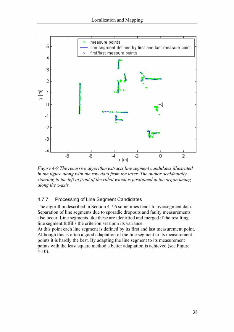
Localization and Mapping
38
Figure 4-9 The recursive algorithm extracts line segment candidates illustrated in the figure along with the raw data from the laser. The author accidentally standing to the left in front of the robot which is positioned in the origin facing along the x-axis.
4.7.7 Processing of Line Segment Candidates The algorithm described in Section 4.7.6 sometimes tends to oversegment data. Separation of line segments due to sporadic dropouts and faulty measurements also occur. Line segments like these are identified and merged if the resulting line segment fulfills the criterion set upon its variance. At this point each line segment is defined by its first and last measurement point. Although this is often a good adaptation of the line segment to its measurement points it is hardly the best. By adapting the line segment to its measurement points with the least square method a better adaptation is achieved (see Figure 4-10).
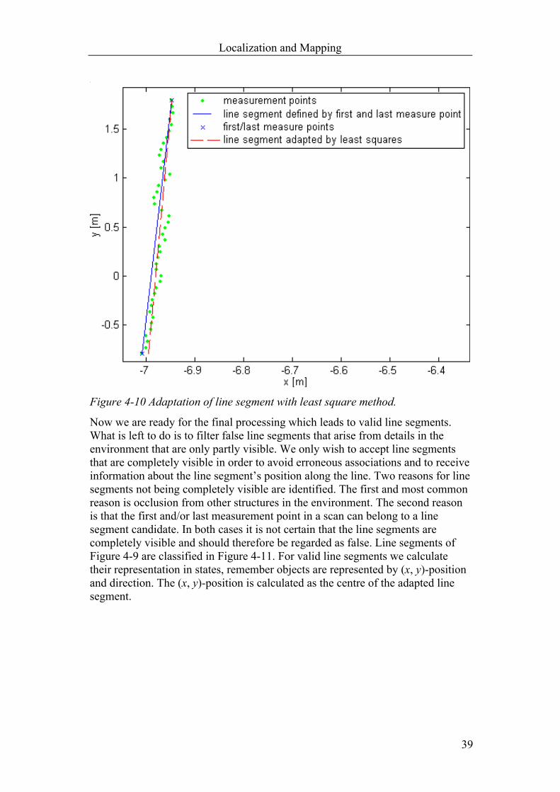
Localization and Mapping
39
Figure 4-10 Adaptation of line segment with least square method.
Now we are ready for the final processing which leads to valid line segments. What is left to do is to filter false line segments that arise from details in the environment that are only partly visible. We only wish to accept line segments that are completely visible in order to avoid erroneous associations and to receive information about the line segment’s position along the line. Two reasons for line segments not being completely visible are identified. The first and most common reason is occlusion from other structures in the environment. The second reason is that the first and/or last measurement point in a scan can belong to a line segment candidate. In both cases it is not certain that the line segments are completely visible and should therefore be regarded as false. Line segments of Figure 4-9 are classified in Figure 4-11. For valid line segments we calculate their representation in states, remember objects are represented by (x, y)-position and direction. The (x, y)-position is calculated as the centre of the adapted line segment.

Localization and Mapping
40
Figure 4-11 Valid and false line segments. The positions of false line segments are also plotted for comparison.
4.7.8 Covariance Matrix for Line Segments The calculation of covariance matrices for line segments is not very different from Hough lines. After all a line segment is very similar to a Hough line, the difference is simply that for line segments we know that we have seen the start- and endpoint. Thus we conclude that the variance for the direction normal to the line segment and the line segments direction is calculated in the same way as for Hough lines. The property of knowing start- and endpoint and the fact that we only use line segments that are not occluded makes them possess information also in position directed along the line. The variance in this direction is calculated by considering that the beams of the laser are sent out in a limited number of directions. As a consequence the start- and endpoint of the actual line will always be missed with some unknown distance. This means that the first and last measurement point belonging to a line will always be interjected on the actual line with some unknown distance ∆start and ∆end (see Figure 4-12).
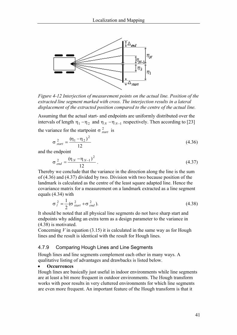
Localization and Mapping
41
Figure 4-12 Interjection of measurement points on the actual line. Position of the extracted line segment marked with cross. The interjection results in a lateral displacement of the extracted position compared to the centre of the actual line.
Assuming that the actual start- and endpoints are uniformly distributed over the intervals of length 21 ηη − and 1−− NN ηη respectively. Then according to [23]
the variance for the startpoint 2startσ is
12)( 2
212 ηησ
−=start (4.36)
and the endpoint
12)( 2
12 −−= NN
endηη
σ . (4.37)
Thereby we conclude that the variance in the direction along the line is the sum of (4.36) and (4.37) divided by two. Division with two because position of the landmark is calculated as the centre of the least square adapted line. Hence the covariance matrix for a measurement on a landmark extracted as a line segment equals (4.34) with
).(21 222
endstartl σσσ += (4.38)
It should be noted that all physical line segments do not have sharp start and endpoints why adding an extra term as a design parameter to the variance in (4.38) is motivated. Concerning V in equation (3.15) it is calculated in the same way as for Hough lines and the result is identical with the result for Hough lines.
4.7.9 Comparing Hough Lines and Line Segments Hough lines and line segments complement each other in many ways. A qualitative listing of advantages and drawbacks is listed below. • Occurrences Hough lines are basically just useful in indoor environments while line segments are at least a bit more frequent in outdoor environments. The Hough transform works with poor results in very cluttered environments for which line segments are even more frequent. An important feature of the Hough transform is that it
Localization and Mapping
42
finds walls even when they are partly occluded by other objects whereas the line segment algorithm splits occluded walls. • Information Hough lines contain much information for line heading and line position in the direction normal to the line. Line segments usually contain less information for line heading and line position in the direction normal to the line. On the other hand line segments also contains information for position in the direction along the line because start- and endpoint are required to be visible. • Computation burden Extracting line segments is computationally faster than extracting Hough walls.
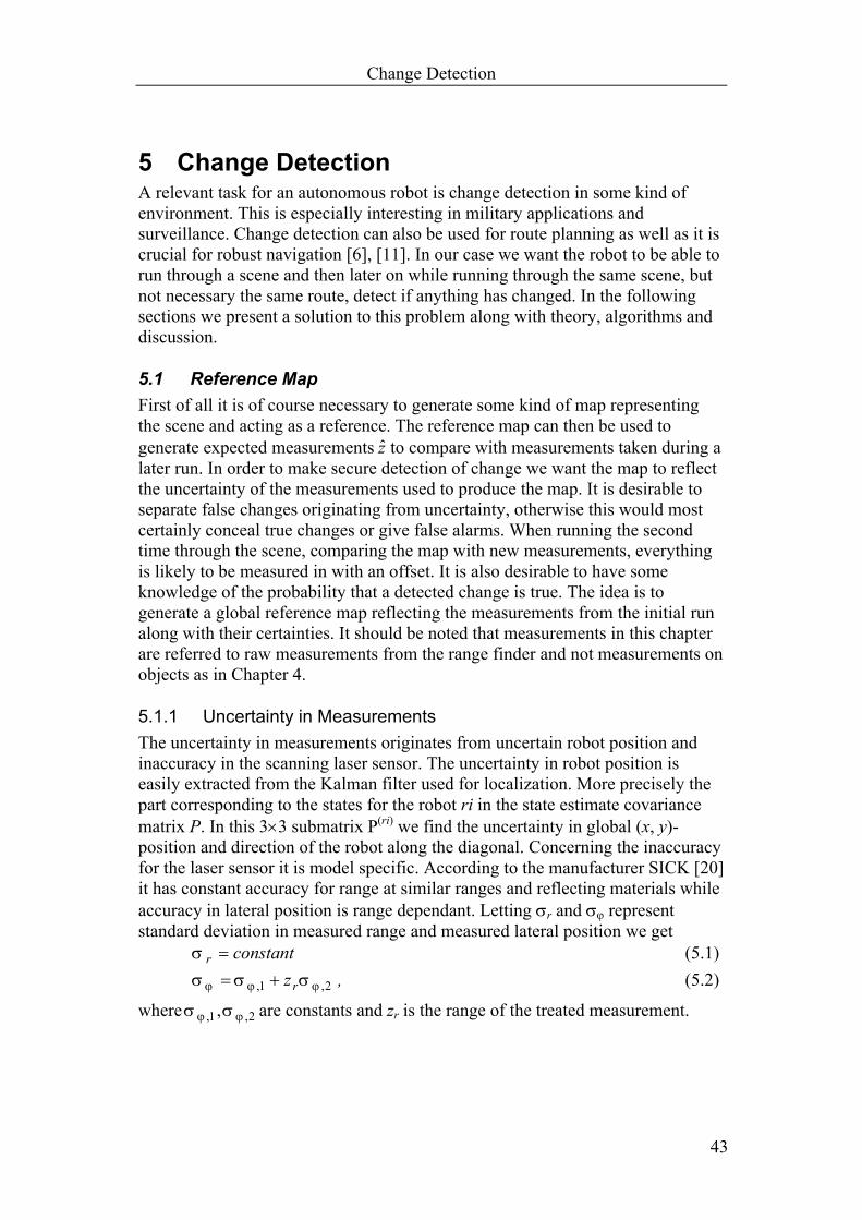
Change Detection
43
5 Change Detection A relevant task for an autonomous robot is change detection in some kind of environment. This is especially interesting in military applications and surveillance. Change detection can also be used for route planning as well as it is crucial for robust navigation [6], [11]. In our case we want the robot to be able to run through a scene and then later on while running through the same scene, but not necessary the same route, detect if anything has changed. In the following sections we present a solution to this problem along with theory, algorithms and discussion.
5.1 Reference Map First of all it is of course necessary to generate some kind of map representing the scene and acting as a reference. The reference map can then be used to generate expected measurements z to compare with measurements taken during a later run. In order to make secure detection of change we want the map to reflect the uncertainty of the measurements used to produce the map. It is desirable to separate false changes originating from uncertainty, otherwise this would most certainly conceal true changes or give false alarms. When running the second time through the scene, comparing the map with new measurements, everything is likely to be measured in with an offset. It is also desirable to have some knowledge of the probability that a detected change is true. The idea is to generate a global reference map reflecting the measurements from the initial run along with their certainties. It should be noted that measurements in this chapter are referred to raw measurements from the range finder and not measurements on objects as in Chapter 4.
5.1.1 Uncertainty in Measurements The uncertainty in measurements originates from uncertain robot position and inaccuracy in the scanning laser sensor. The uncertainty in robot position is easily extracted from the Kalman filter used for localization. More precisely the part corresponding to the states for the robot ri in the state estimate covariance matrix P. In this 3×3 submatrix P(ri) we find the uncertainty in global (x, y)-position and direction of the robot along the diagonal. Concerning the inaccuracy for the laser sensor it is model specific. According to the manufacturer SICK [20] it has constant accuracy for range at similar ranges and reflecting materials while accuracy in lateral position is range dependant. Letting σr and σϕ represent standard deviation in measured range and measured lateral position we get
antconstr =σ (5.1) ,z r 2,1, ϕϕϕ σσσ += (5.2)
where 2,1, , ϕϕ σσ are constants and zr is the range of the treated measurement.

Change Detection
44
Figure 5-1 The effect of inaccuracy in the measuring laser.
Another term that affects the total uncertainty for a measured point in the same way as σϕ,2 in (5.2) is the standard deviation of the robots direction )(ri
ϕσ , i.e. the
square root of element 3,3 in P(ri). This term should be added to σϕ in (5.2) revealing a part (covpart) of the total covariance matrix for the measurement by considering a local coordinate system with x- and y-axis parallel to σr and σϕ in Figure 5-1.
( )
++= 2)(
2,1,
2
)(0
0cov ri
r
rpart z ϕϕϕ σσσ
σ (5.3)
As mentioned covpart is not the total uncertainty for the measurement. The total uncertainty involves the uncertainties of the measuring robots global (x,y)-position. Before we can add this term we need to transform covpart to global coordinates. It is done in two steps, first to the robot relative xri, yri and then to the global coordinate system xg, yg. The first rotation matrix is given by the angle of the measurement zϕ, the second is given by the estimated direction of the robot )(ˆ rixϕ .
−=
)cos()sin()sin()cos(
)(ϕϕ
ϕϕϕ zz
zzzM (5.4)
−=
)ˆcos()ˆsin()ˆsin()ˆcos(
)ˆ( )()(
)()()(
riri
ririri
xxxx
xMϕϕ
ϕϕϕ (5.5)
After rotating covpart we need only to add the submatrix in P(ri) that corresponds to the variance and covariance for x- and y-position of the robot. This submatrix of P(ri) is given by elements 1:2 in rows 1:2 and thus with Matlab notation the total covariance of a measurement becomes
+= TriTpart
ri xMzMzMxM(z) )ˆ()(cov)()ˆ(cov )()(ϕϕϕϕ
).2:1,2:1()(riP+ (5.6) A graphical illustration of (5.6) can be viewed in Figure 5-2.
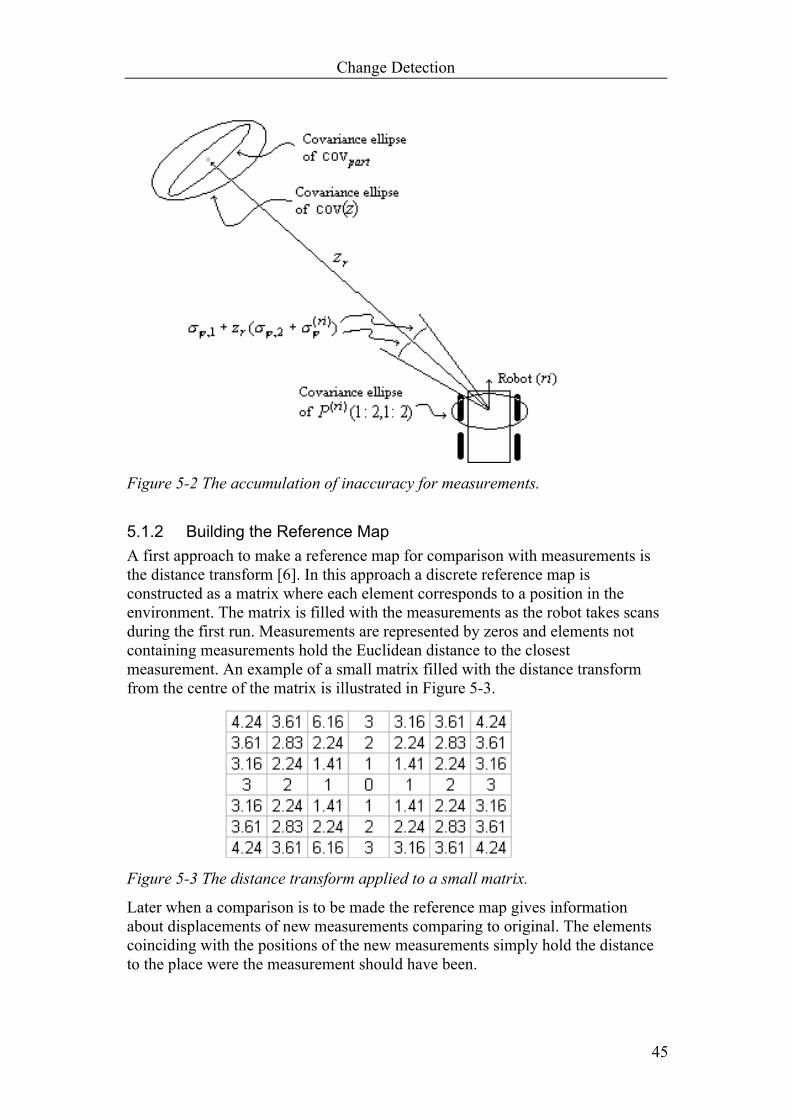
Change Detection
45
Figure 5-2 The accumulation of inaccuracy for measurements.
5.1.2 Building the Reference Map A first approach to make a reference map for comparison with measurements is the distance transform [6]. In this approach a discrete reference map is constructed as a matrix where each element corresponds to a position in the environment. The matrix is filled with the measurements as the robot takes scans during the first run. Measurements are represented by zeros and elements not containing measurements hold the Euclidean distance to the closest measurement. An example of a small matrix filled with the distance transform from the centre of the matrix is illustrated in Figure 5-3.
Figure 5-3 The distance transform applied to a small matrix.
Later when a comparison is to be made the reference map gives information about displacements of new measurements comparing to original. The elements coinciding with the positions of the new measurements simply hold the distance to the place were the measurement should have been.
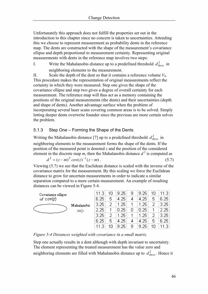
Change Detection
46
Unfortunately this approach does not fulfill the properties set out in the introduction to this chapter since no concern is taken to uncertainties. Attending this we choose to represent measurement as probability dents in the reference map. The dents are constructed with the shape of the measurement’s covariance ellipse and depth proportional to measurement certainty. Representing original measurements with dents in the reference map involves two steps: I. Write the Mahalanobis distance up to a predefined threshold 2
thresd in neighboring elements to the measurement.
II. Scale the depth of the dent so that it contains a reference volume V0. This procedure makes the representation of original measurements reflect the certainty in which they were measured. Step one gives the shape of the covariance ellipse and step two gives a degree of overall certainty for each measurement. The reference map will thus act as a memory containing the positions of the original measurements (the dents) and their uncertainties (depth and shape of dents). Another advantage surface when the problem of incorporating several laser scans covering common areas is to be solved. Simply letting deeper dents overwrite founder since the previous are more certain solves the problem.
5.1.3 Step One – Forming the Shape of the Dents
Writing the Mahalanobis distance [7] up to a predefined threshold 2thresd in
neighboring elements to the measurement forms the shape of the dents. If the position of the measured point is denoted z and the position of the considered element in the discrete map m, then the Mahalanobis distance d 2 is computed as
)()()( 12 mzzcovmzd T −−= − . (5.7) Viewing (5.7) we see that the Euclidean distance is scaled with the inverse of the covariance matrix for the measurement. By this scaling we force the Euclidean distance to grow for uncertain measurements in order to indicate a similar separation compared to a more certain measurement. An example of resulting distances can be viewed in Figure 5-4.
Figure 5-4 Distances weighted with covariance in a small matrix.
Step one actually results in a dent although with depth invariant to uncertainty. The element representing the treated measurement has the value zero and neighboring elements are filled with Mahalanobis distance up to 2
thresd . Hence it
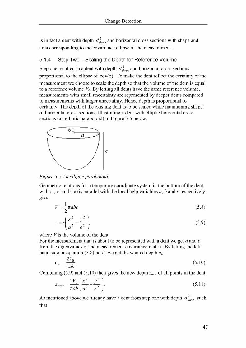
Change Detection
47
is in fact a dent with depth 2thresd and horizontal cross sections with shape and
area corresponding to the covariance ellipse of the measurement.
5.1.4 Step Two – Scaling the Depth for Reference Volume
Step one resulted in a dent with depth 2thresd and horizontal cross sections
proportional to the ellipse of ).cov(z To make the dent reflect the certainty of the measurement we choose to scale the depth so that the volume of the dent is equal to a reference volume V0. By letting all dents have the same reference volume, measurements with small uncertainty are represented by deeper dents compared to measurements with larger uncertainty. Hence depth is proportional to certainty. The depth of the existing dent is to be scaled while maintaining shape of horizontal cross sections. Illustrating a dent with elliptic horizontal cross sections (an elliptic paraboloid) in Figure 5-5 below.
Figure 5-5 An elliptic paraboloid.
Geometric relations for a temporary coordinate system in the bottom of the dent with x-, y- and z-axis parallel with the local help variables a, b and c respectively give:
abcV π21
= (5.8)
,2
2
2
2
+=
by
axcz (5.9)
where V is the volume of the dent. For the measurement that is about to be represented with a dent we get a and b from the eigenvalues of the measurement covariance matrix. By letting the left hand side in equation (5.8) be V0 we get the wanted depth cw,
abV
cw π02
= . (5.10)
Combining (5.9) and (5.10) then gives the new depth znew of all points in the dent
+=
2
2
2
202
by
ax
abV
znew π. (5.11)
As mentioned above we already have a dent from step one with depth 2thresd such
that
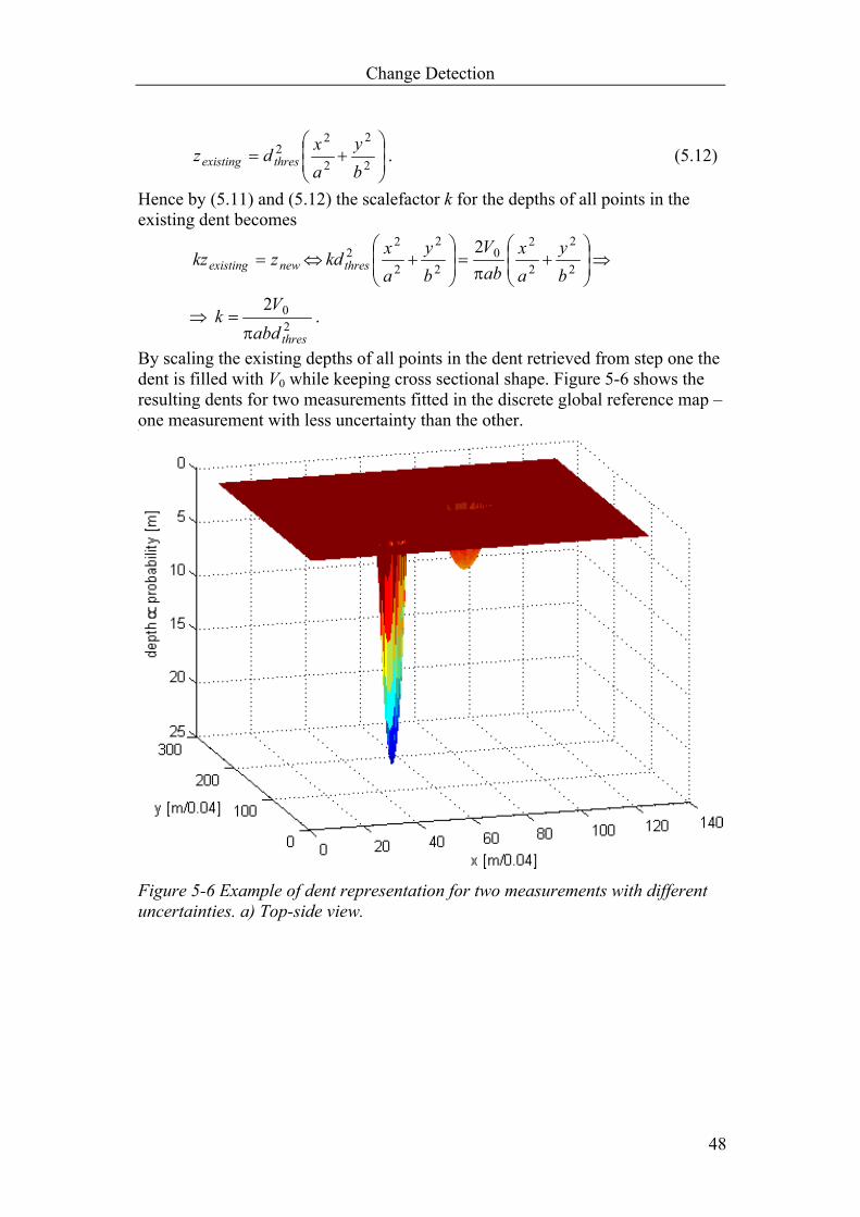
Change Detection
48
+=
2
2
2
22
by
axdz thresexisting . (5.12)
Hence by (5.11) and (5.12) the scalefactor k for the depths of all points in the existing dent becomes
newexisting zkz = ⇔
+=
+
2
2
2
20
2
2
2
22 2
by
ax
abV
by
axkdthres π
⇒
⇒ 202
thresabdV
kπ
= .
By scaling the existing depths of all points in the dent retrieved from step one the dent is filled with V0 while keeping cross sectional shape. Figure 5-6 shows the resulting dents for two measurements fitted in the discrete global reference map – one measurement with less uncertainty than the other.
Figure 5-6 Example of dent representation for two measurements with different uncertainties. a) Top-side view.
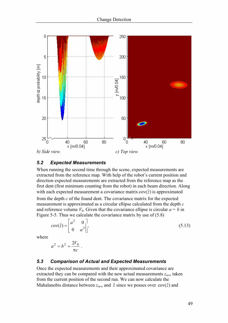
Change Detection
49
b) Side view. c) Top view.
5.2 Expected Measurements When running the second time through the scene, expected measurements are extracted from the reference map. With help of the robot’s current position and direction expected measurements are extracted from the reference map as the first dent (first minimum counting from the robot) in each beam direction. Along with each expected measurement a covariance matrix )ˆcov(z is approximated from the depth c of the found dent. The covariance matrix for the expected measurement is approximated as a circular ellipse calculated from the depth c and reference volume V0. Given that the covariance ellipse is circular a = b in Figure 5-5. Thus we calculate the covariance matrix by use of (5.8)
,0
0)ˆ( 2
2
=
aazcov (5.13)
where
cV
baπ
022 2== .
5.3 Comparison of Actual and Expected Measurements Once the expected measurements and their approximated covariance are extracted they can be compared with the new actual measurements znew taken from the current position of the second run. We can now calculate the Mahalanobis distance between znew and z since we posses over )ˆcov(z and
Change Detection
50
cov(znew) is derived according to Section 5.1.1. The Mahalanobis distance d 2 is computed for each new measurement point and its corresponding expected measurement point. Thereby accounting for uncertainty in both the expected (reference) and the new measurement.
)ˆ())ˆ()(()ˆ( 12 zzzcovzcovzzd newnewT
new −+−= − (5.14) A proper threshold, for which the Mahalanobis distance between znew and z has to exceed in order to be seen as an interesting change, is set. Equation (5.14) along with the occlusion maps (see Section 5.4) constitute the basis for the change detection algorithm. Direct comparison of two measurements (one expected and one new) yields sensitive performance. Experiments conclude that false detection of change occur when sporadic beams are not reflected or reflected in the wrong way. This can happen when the surface of an obstacle has bad reflectivity or very good reflectivity. In the first case the beam is not returned leaving the range unknown. In the second case the beam is not reflected back to the sensor but in another direction resulting in two possibilities: reflecting on another obstacle or not reflecting at all. In both cases wrong information is brought to the sensor. Some of these false alarms can be avoided by processing the data. One idea would be to add the constraint that the Mahalanobis distance should exceed the threshold for a number of consecutive measurement points in order to be viewed as a change. An optional and more extensive processing of data would be to demand measurements on the environment to be stable over time before adding them to the reference map or using them for comparison. In this way sporadic incorrectly reflected and not reflected measurements can be avoided as well as temporary changes due to for instance wind. However depending on the application this might not be the best approach, imagine as an example that moving objects are desirable to detect.
5.4 Occlusion Map Another problem that needs attention is the problem of occlusion [10]. Objects that were occluded when constructing the reference map may be visible from another position when taking measurements for comparison. If this is the case then the new measurement is located in an area that was occluded for the robot when taking reference measurements. Hence the change detection algorithm should not indicate change because the structure giving the new measurement may very well have been there in the first place. A situation like this is illustrated in Figure 5-7.

Change Detection
51
Figure 5-7 Structure visible from the new position but occluded when the reference scan was taken.
Without proper algorithms, such a situation would indicate false alarms. The problem is attended by building an occlusion map for the reference map. The occlusion map is basically ones and zeros. Zeros in elements beyond objects (occluded areas) and ones in elements on this, from the robots view, side of objects (visible areas) including the objects themselves and their uncertain extensions. An example of an occlusion map can be viewed in Figure 5-8 below. The observant viewer sees that the occlusion map contains some small islands of black and white. This is of course not correct but a consequence of the limited resolution.
Figure 5-8 a) An occlusion map illustrating visible (white) and occluded areas (black). Robot standing on x-axis at x = 80 facing upward.

Change Detection
52
b) The measurements from which the occlusion map in Figure 5-8 a) was built. Robot standing on x-axis at x = 80 facing upward.
False alarms due to occlusion are avoided by consulting the occlusion map. When the algorithm detects change in some region the occlusion map is consulted. The detected change is then considered false if the region of the new measurement is occluded and in front of the expected measurement.
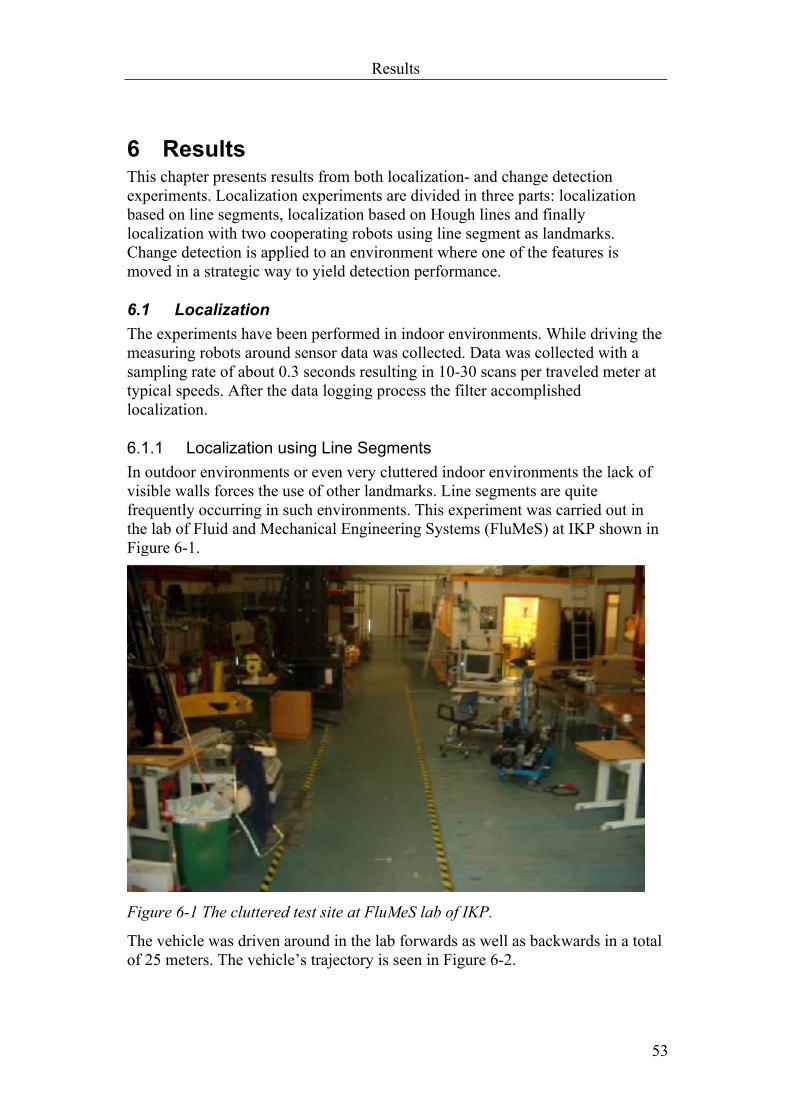
Results
53
6 Results This chapter presents results from both localization- and change detection experiments. Localization experiments are divided in three parts: localization based on line segments, localization based on Hough lines and finally localization with two cooperating robots using line segment as landmarks. Change detection is applied to an environment where one of the features is moved in a strategic way to yield detection performance.
6.1 Localization The experiments have been performed in indoor environments. While driving the measuring robots around sensor data was collected. Data was collected with a sampling rate of about 0.3 seconds resulting in 10-30 scans per traveled meter at typical speeds. After the data logging process the filter accomplished localization.
6.1.1 Localization using Line Segments In outdoor environments or even very cluttered indoor environments the lack of visible walls forces the use of other landmarks. Line segments are quite frequently occurring in such environments. This experiment was carried out in the lab of Fluid and Mechanical Engineering Systems (FluMeS) at IKP shown in Figure 6-1.
Figure 6-1 The cluttered test site at FluMeS lab of IKP.
The vehicle was driven around in the lab forwards as well as backwards in a total of 25 meters. The vehicle’s trajectory is seen in Figure 6-2.
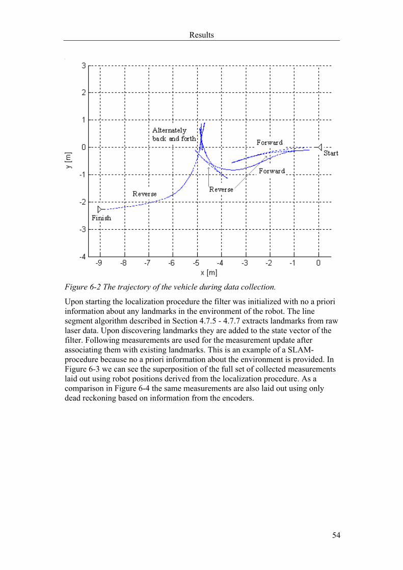
Results
54
Figure 6-2 The trajectory of the vehicle during data collection.
Upon starting the localization procedure the filter was initialized with no a priori information about any landmarks in the environment of the robot. The line segment algorithm described in Section 4.7.5 - 4.7.7 extracts landmarks from raw laser data. Upon discovering landmarks they are added to the state vector of the filter. Following measurements are used for the measurement update after associating them with existing landmarks. This is an example of a SLAM-procedure because no a priori information about the environment is provided. In Figure 6-3 we can see the superposition of the full set of collected measurements laid out using robot positions derived from the localization procedure. As a comparison in Figure 6-4 the same measurements are also laid out using only dead reckoning based on information from the encoders.

Results
55
Figure 6-3 Superposition of the 350 collected range scans using localization.
Figure 6-4 Superposition of the 350 collected range scans using dead reckoning.

Results
56
Figure 6-3 and Figure 6-4 clearly shows the benefit of localization using landmarks. Measurements on solid features such as walls are much more held together in Figure 6-3 using the SLAM technique. Measurements are more held together because they are laid out using the vehicle’s global position estimate which is better at all times when using SLAM. It should be noted that the feature at x = -6 and y = -3.5 was moved during the data collection why it looks blurred also in Figure 6-3. In order to give a more exact size of the benefit from localization with landmarks one can take a more close view on a feature such as the corner of two walls. A corner is a good measure because it confirms that certainty of the measuring robot has been maintained in all directions. The corner at x = -6 and y = -0.5 is visible during most of the data collection.
Figure 6-5 Enlargement of the corner at x = -6 and y = -0.5 in Figure 6-3 (using localization with landmarks).

Results
57
Figure 6-6 Enlargement of the corner at x = -6 and y = -0.5 in Figure 6-4 (using only dead reckoning).
Worth noting is that a large board was leaning towards left wall of the corner at the time of the experiment. Figure 6-5 and Figure 6-6 shows that the scattering of measurements is in the order of 5 cm for the case of localization and 20 cm for dead reckoning. Reflecting over this one should have in mind that the standard deviation of the range finding laser is in the order of centimeters. In Figure 6-7 the extracted and used landmarks are shown along with the superposition of some scans that cover the lab. Viewing Figure 6-7 we see that the line segment algorithm extracts straight physical line segments that are completely visible and not occluded by other features.

Results
58
Figure 6-7 The extracted and used landmarks marked with rings along with superposition of a few scans taken at marked positions. The scans have been laid out using the filtered positions.
6.1.2 Localization using Hough Lines In fairly clean indoor environments landmarks extracted with the Hough transform can be used for localization with good results. In such environments walls are especially useful because they contain much information. This experiment was carried out in the B-building of Linköping University Campus Valla. Starting point was the FluMeS lab facing out towards the corridor. The vehicle was driven about 60 m down the corridor followed by a right turn in the crossing corridor, 20 m down this corridor it was turned and driven back to the starting position. Starting and finishing in same place is a good idea because then, after applying localization with landmarks, we will find out if the filter has succeeded to estimate true positions. In order to make the localization even more difficult a two-percent error was added to the calibrated radius of one wheel. Upon starting the localization procedure the filter was initialized with no a priori information about any landmarks in the environment of the robot. The Hough transform described in Section 4.7.1 - 4.7.3 extracts Hough lines from raw laser data. Upon discovering landmarks they are added to the state vector of the filter. Following measurements are used for the measurement update after associating them with existing landmarks. This is an example of a SLAM-procedure because
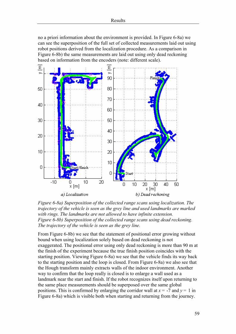
Results
59
no a priori information about the environment is provided. In Figure 6-8a) we can see the superposition of the full set of collected measurements laid out using robot positions derived from the localization procedure. As a comparison in Figure 6-8b) the same measurements are laid out using only dead reckoning based on information from the encoders (note: different scale).
Figure 6-8a) Superposition of the collected range scans using localization. The trajectory of the vehicle is seen as the grey line and used landmarks are marked with rings. The landmarks are not allowed to have infinite extension. Figure 6-8b) Superposition of the collected range scans using dead reckoning. The trajectory of the vehicle is seen as the grey line.
From Figure 6-8b) we see that the statement of positional error growing without bound when using localization solely based on dead reckoning is not exaggerated. The positional error using only dead reckoning is more than 90 m at the finish of the experiment because the true finish position coincides with the starting position. Viewing Figure 6-8a) we see that the vehicle finds its way back to the starting position and the loop is closed. From Figure 6-8a) we also see that the Hough transform mainly extracts walls of the indoor environment. Another way to confirm that the loop really is closed is to enlarge a wall used as a landmark near the start and finish. If the robot recognizes itself upon returning to the same place measurements should be superposed over the same global positions. This is confirmed by enlarging the corridor wall at x = -7 and y = 1 in Figure 6-8a) which is visible both when starting and returning from the journey.

Results
60
Figure 6-9 Enlargement of the corridor wall at x = -7 and y = 1 in Figure 6-8a) (using localization). The grey dots are the estimated positions of the vehicle as it starts and returns from its journey.
6.1.3 Localization using two Robots The main benefits of cooperating robots can be expected to arise in environments containing few landmarks. In such environments cooperating robots can move through the terrain with strategies that reduce their overall position uncertainty. A strategy would be to move one by one. As one robot moves the other is stationary measuring the movement of the other robot. The following experiment was designed so that the Pioneer moved while using only one landmark. As the Pioneer moved the vehicle stood stationary delivering measurements of the Pioneer’s position at every sampling time. Comparing localization performed with and without help of the vehicle isolates the effect from cooperation. The results are presented in Figure 6-10 - Figure 6-13. In Figure 6-10 we see the superposed measurements from the Pioneer when it localizes itself only by use of the single landmark and without help of the vehicle. As a comparison in Figure 6-11 we see the same measurements superposed from positions derived by use of the single landmark and additional aid from the cooperating vehicle.
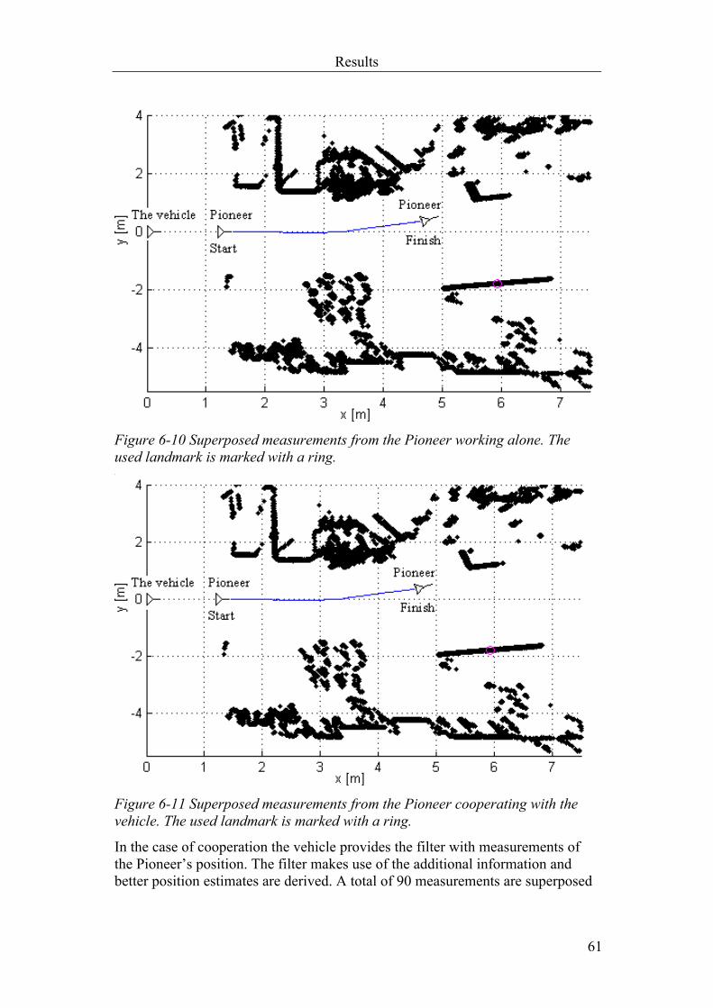
Results
61
Figure 6-10 Superposed measurements from the Pioneer working alone. The used landmark is marked with a ring.
Figure 6-11 Superposed measurements from the Pioneer cooperating with the vehicle. The used landmark is marked with a ring.
In the case of cooperation the vehicle provides the filter with measurements of the Pioneer’s position. The filter makes use of the additional information and better position estimates are derived. A total of 90 measurements are superposed

Results
62
in the figures. From Figure 6-10 and Figure 6-11 the benefit from cooperation may not be directly visible. However, enlarging the structure at x = 5.5 and y = 1.5 reveals an obvious improvement seen in Figure 6-12 and Figure 6-13.
Figure 6-12 Enlargement of the structure at x = 5.5 and y = 1.5 in Figure 6-10 (without cooperation).
Figure 6-13 Enlargement of the structure at x = 5.5 and y = 1.5 in Figure 6-11 (with cooperation).
Measurements are more held together in Figure 6-13 comparing to Figure 6-12 because they are laid out using the Pioneer’s global position estimates which are better at all times when the robots cooperate.
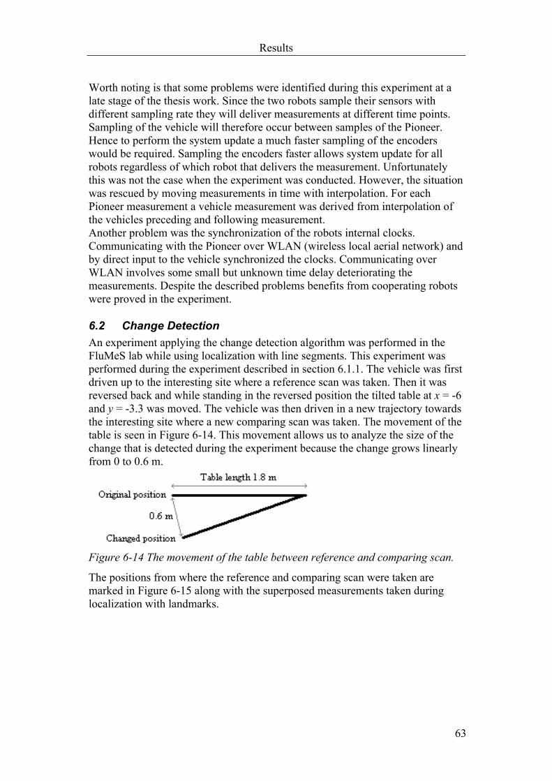
Results
63
Worth noting is that some problems were identified during this experiment at a late stage of the thesis work. Since the two robots sample their sensors with different sampling rate they will deliver measurements at different time points. Sampling of the vehicle will therefore occur between samples of the Pioneer. Hence to perform the system update a much faster sampling of the encoders would be required. Sampling the encoders faster allows system update for all robots regardless of which robot that delivers the measurement. Unfortunately this was not the case when the experiment was conducted. However, the situation was rescued by moving measurements in time with interpolation. For each Pioneer measurement a vehicle measurement was derived from interpolation of the vehicles preceding and following measurement. Another problem was the synchronization of the robots internal clocks. Communicating with the Pioneer over WLAN (wireless local aerial network) and by direct input to the vehicle synchronized the clocks. Communicating over WLAN involves some small but unknown time delay deteriorating the measurements. Despite the described problems benefits from cooperating robots were proved in the experiment.
6.2 Change Detection An experiment applying the change detection algorithm was performed in the FluMeS lab while using localization with line segments. This experiment was performed during the experiment described in section 6.1.1. The vehicle was first driven up to the interesting site where a reference scan was taken. Then it was reversed back and while standing in the reversed position the tilted table at x = -6 and y = -3.3 was moved. The vehicle was then driven in a new trajectory towards the interesting site where a new comparing scan was taken. The movement of the table is seen in Figure 6-14. This movement allows us to analyze the size of the change that is detected during the experiment because the change grows linearly from 0 to 0.6 m.
Figure 6-14 The movement of the table between reference and comparing scan.
The positions from where the reference and comparing scan were taken are marked in Figure 6-15 along with the superposed measurements taken during localization with landmarks.

Results
64
Figure 6-15 Trajectory of robot and positions from where the reference and comparing scan were taken.
The reference scan is used to build a reference map described in Section 5.1. Expected measurements are extracted from the reference map and they are used for comparison with measurements of the comparing scan. If nothing in environment has changed between the reference scan and the comparing scan then expected measurements should concur with measurements in the comparing scan. The original measurements of the reference scan and the expected measurements extracted from the reference map are seen in Figure 6-16. Measurements of the comparing scan are seen with the expected measurements in Figure 6-17.
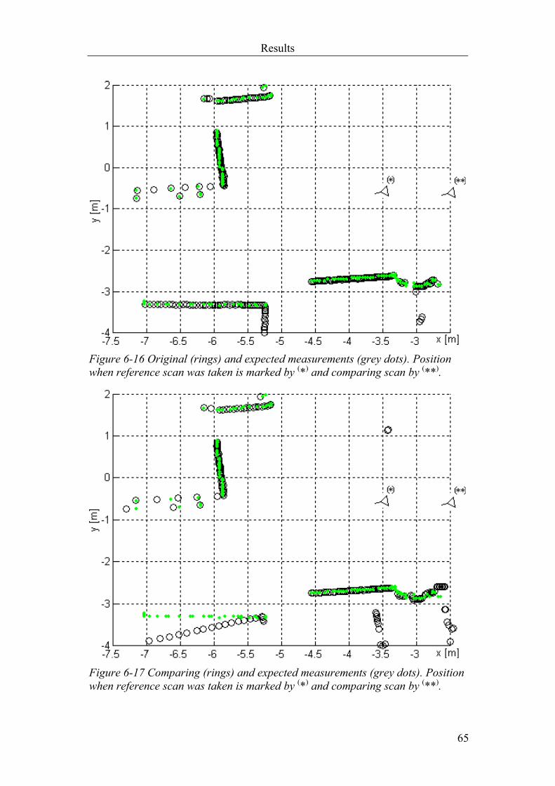
Results
65
Figure 6-16 Original (rings) and expected measurements (grey dots). Position when reference scan was taken is marked by (*) and comparing scan by (**).
Figure 6-17 Comparing (rings) and expected measurements (grey dots). Position when reference scan was taken is marked by (*) and comparing scan by (**).

Results
66
Changes in the environment are now detected by comparing expected measurements extracted from the reference map with corresponding measurements of the comparing scan. Applying (5.14) and setting the threshold with margin well over the threshold used when associating objects in the localization procedure yields the result in Figure 6-18.
Figure 6-18 Expected measurements separated from comparing new measurements with Mahalanobis distance greater than the threshold are marked with rings. Expected measurements separated with Mahalanobis distance less then the threshold are marked with dots
The result yields consecutive changes at the moved table but also sporadic false changes in other places. The smallest detected actual displacement of the table is just over 5 cm. Except for the lower limit set by the resolution of the reference map the ability of detecting small changes is more a question of how good the robot can localize itself during surveillance than the change detection algorithm itself. This is a consequence of the demands set upon the change detection algorithm. The change detection algorithm was designed to detect changes when comparing measurements taken from different positions while accounting for measurement uncertainties.

Conclusions and Future Work
67
7 Conclusions and Future Work In this chapter conclusions and proposition of future work are presented. Conclusions are drawn from the implemented algorithms and performed experiments. Future work is proposed based on experiences from this master thesis.
7.1 Conclusions Starting with a Kalman filter strictly used for localization of simulated mobile robots and landmarks a modified version has been developed taking in experimental sensor data. Sensor data has been collected with moving sensor platforms (mobile robots) equipped with laser range finder and wheel revolution counters. Data has been collected from robot movements in natural environments and localization is applied after the collection has finished, i.e. not in real-time. Adapting the simulation filter to experimental sensor data mainly included developing: • Robot motion model (process model) including process noise • Methods to extract natural landmarks from raw range sensor data along with
noise for measurements upon landmarks • Method to associate existing objects with new measurements • Method to add new objects (landmarks) to the Kalman filter The modified filter has been tested in both very cluttered and fairly clean environments using two types of landmarks. The tests prove good results localizing the robot with positional uncertainty within the order of centimeters. Comparisons with localization based on wheel revolution counters alone show tremendous improvement. Additionally cooperation between two robots is tested in a scenario where benefits can be expected from cooperation. Despite encountered time synchronization problems and need for higher encoder sampling rate cooperation proved advantageous. A common autonomous robot task was also implemented in the form change detection. The goal of the change detection algorithm was that it should account for robot position- and measurement uncertainty when detecting change in the environment. The problem was solved by building a global discrete reference map acting as a memory both for measurement positions and measurement uncertainties. The reference map is later used to extract expected measurements that are compared with new measurements with help of the Mahalanobis distance. The change detection algorithm also presented a systematic way of treating the issue of occlusion which otherwise can lead to false alarms. Change detection was tested while also applying localization. Given the presence of a sufficient number of landmarks, changes just over 5 cm were detected. Additionally sporadic false changes were also detected mostly due to spurious beam reflections. Post processing was proposed as a solution to this.
Conclusions and Future Work
68
7.2 Future Work The subject of autonomous mobile robots is very interesting and much work remains. During this master thesis many problems were encountered that require extensive investigation and work although not treated here. The limitations of this master thesis are of course also subject to future work. Listed below are some propositions of future work with described problems. • Path- and task planning Autonomous robots must be able to solve problems given to them without detailed instructions. A prerequisite is path planning since most tasks for mobile robots involve movement between positions. An interesting question is also how several robots are to cooperate in order to minimize positional uncertainties? • Introduce three dimensional space In outdoor applications it is not possible to maintain the assumption of two-dimensional space. Introducing three dimensions require additional sensors and modified models. • Real-time Implement the localization for real-time applications. To fully test the performance of the centralized Kalman filter for cooperating robots tests should be performed in real-time. This also introduces the problem of time synchronization when using wireless network communication between the robots. • Additional landmarks Localization in outdoor environments requires other landmarks than Hough lines and line segments. Frequent objects may be vertical cylinders such as trees and poles. The localization procedure can also be made invariant to varying environments by adding the ability to use several kinds of landmarks. • Robustness against erroneous associations The risk of erroneous associations between measurements and existing objects can not be neglected. The consequence of a single erroneous association is severe. Without detection and correction the robot will lose track of its own position and is likely to never regain track once an erroneous association has occurred. Other association methods than NNSF can be tested. More advanced association methods may be better in the sense of avoiding erroneous associations. • Alternative filtering methods Other filtering methods may be better alternatives then extended Kalman filtering. Which filtering method fits the application best? Alternatives are particle filtering and interactive multiple models (IMM) among others.

Conclusions and Future Work
69
• Extensive simulations More extensive simulations can be performed to yield important theoretical results. Statistics on filtering stability, lower bound of estimation uncertainty and quantitative comparisons of different filtering methods are some examples of important areas. • Decentralized approach An alternative to the centralized Kalman filter approach treating landmarks and cooperating robots could be a decentralized approach. An expected benefit is the reduced amount of data transfer between robots and the central processing unit.
70
References [1] F. Gustafsson, L. Ljung, M. Millnert, Signalbehandling,
Studentlitteratur, 2001 [2] J. Borenstein, L. Feng, Measurement and Correction of Systematic
Odometry Errors in Mobile Robots, IEEE Journal of Robotics and Automation, Dec 1996
[3] A. Persson, L-C. Böiers, Flervariabel analys, Studentlitteratur, 1988 [4] U. Larsson, On Robot Control with Feedback from Optronic Sensors,
Doctoral thesis, LuTH, 1999 [5] I. Cox, G. Wilfong, Autonomous Robot Vehicles, Springer Verlag, 1990 [6] P. L. Klöör, P. Lundquist, P. Ohlsson, J. Nygårds, Å. Wernersson,
Change detection in natural scenes using laser range measurements from a mobile robot, IFAC, 1993
[7] K. Mardia, J. Kent, J. Bibby, Multivariate Analysis, Academic Press, 1989
[8] L. Zhang, B. Ghosh, Line Segment Based Map Building and Localization Using 2D Laser Rangefinder, IEEE conference on Robotics & Automation in San Francisco, 2000
[9] P. Jensfelt, Approaches to Mobile Robot Localization in Indoor Environments, Doctoral thesis, KTH, 2001
[10] T. Ikegami, J. Kato, S. Ozono, Sensor Data Integration Based on the Border Distance Model, IEEE Workshop, 1989
[11] T. Ikegami, S. Ozono, A New Path Planning Method for Mobile Robots Applicable to an Arbitrary Environment, IEEE conference, 1992 [12] A. Persson, L-C. Böiers, Envariabel analys, Studentlitteratur, 1990 [13] Y. Bar-Shalom, T. Fortman, Tracking and Data Association, volume
179 of Mathematics in Science and Engineering, Academic Press, 1988 [14] I. Roumeliotis, A. Bekey, A distributed Kalman filter approach to
localization of groups of mobile robots, IEEE conference on Robotics & Automation in San Francisco, 2000
[15] I. Rekleitis, R. Sim, G. Dudek, E. Milios, Collaborative exploration for the construction of visual maps, IEEE/RSJ conference on Intelligent Robots and Systems, 2001
[16] ActivMedia Robotics, www.activmedia.com, May 1, 2003 [17] R. Kalman, A new approach to linear filtering and prediction problems,
Journal of Basic Engineering, pp. 35-44, 1960 [18] B. Anderson, J. Moore, Optimal Filtering, Prentice-Hall, 1979 [19] QNX Software Systems LTD, www.qnx.com, May 1, 2003 [20] SICK AG, www.sick.de, May 1, 2003 [21] J. Forsberg, U. Larsson, Å. Wernersson. Mobile Robot Navigation
Using the Range-Weighted Hough Transform, IEEE Robotics & Automation Magazine special issue on Mobile Robots, pp. 18-26, March 1995

71
[22] J. Nygårds, Å. Wernersson, On Covariances for Fusing Laser Rangers and Vision with Sensors Onboard a Moving Robot, Proceedings IEEE/RSJ conference on Intelligent Robots and Systems, 1998
[23] G. Blom, Sannolikhetsteori och statistik med tillämpningar, Studentlitteratur, 2000
[24] J. Kjellander, Sensorfusion med 2 koordinerade farkoster (preliminary title), Master thesis to be published, LiTH-ISY, 2003
[25] B. Stroustrup, The C++ Programming Language, Addison-Wesley, 3rd edition
[26] L. Andersson, J. Nygårds, On Sensor Fusion Between a Pair of Heterogeneous Robots, to be presented at FUSION, 2003
[27] J. Göransson, Restoring Track Driven Robotics Platform to Operational Status (preliminary title), Master thesis to be published, LiTH-IKP, 2003
På svenska Detta dokument hålls tillgängligt på Internet – eller dess framtida ersättare – under en längre tid från publiceringsdatum under förutsättning att inga extra-ordinära omständigheter uppstår.
Tillgång till dokumentet innebär tillstånd för var och en att läsa, ladda ner, skriva ut enstaka kopior för enskilt bruk och att använda det oförändrat för ickekommersiell forskning och för undervisning. Överföring av upphovsrätten vid en senare tidpunkt kan inte upphäva detta tillstånd. All annan användning av dokumentet kräver upphovsmannens medgivande. För att garantera äktheten, säkerheten och tillgängligheten finns det lösningar av teknisk och administrativ art.
Upphovsmannens ideella rätt innefattar rätt att bli nämnd som upphovsman i den omfattning som god sed kräver vid användning av dokumentet på ovan beskrivna sätt samt skydd mot att dokumentet ändras eller presenteras i sådan form eller i sådant sammanhang som är kränkande för upphovsmannens litterära eller konstnärliga anseende eller egenart.
För ytterligare information om Linköping University Electronic Press se förlagets hemsida http://www.ep.liu.se/ In English The publishers will keep this document online on the Internet - or its possible replacement - for a considerable time from the date of publication barring exceptional circumstances.
The online availability of the document implies a permanent permission for anyone to read, to download, to print out single copies for your own use and to use it unchanged for any non-commercial research and educational purpose. Subsequent transfers of copyright cannot revoke this permission. All other uses of the document are conditional on the consent of the copyright owner. The publisher has taken technical and administrative measures to assure authenticity, security and accessibility.
According to intellectual property law the author has the right to be mentioned when his/her work is accessed as described above and to be protected against infringement.
For additional information about the Linköping University Electronic Press and its procedures for publication and for assurance of document integrity, please refer to its WWW home page: http://www.ep.liu.se/ © [Per Holmberg]