strucutural vibrations

7/23/2019 Strucutural Vibrations

http://slidepdf.com/reader/full/strucutural-vibrations 1/14

.

16Modeling for StructuralVibrations: FEM Models,Damping, Similarity Laws

16–1



Chapter 16: MODELING FOR STRUCTURAL VIBRATIONS: FEM MODELS, DAMPING, SIMILARITY L16–2

§16.1 FINITE ELEMENT MODELING OF VIBRATION PROBLEMS

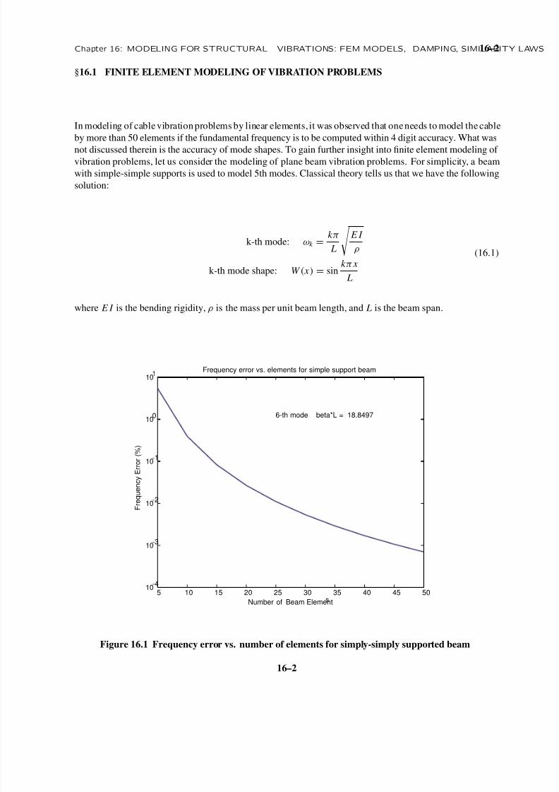
In modeling of cable vibration problems by linear elements, it was observed that one needs to model the cable

by more than 50 elements if the fundamental frequency is to be computed within 4 digit accuracy. What wasnot discussed therein is the accuracy of mode shapes. To gain further insight into finite element modeling of

vibration problems, let us consider the modeling of plane beam vibration problems. For simplicity, a beam

with simple-simple supports is used to model 5th modes. Classical theory tells us that we have the following

solution:

k-th mode: ωk =k π

L

E I

ρ

k-th mode shape: W ( x )=

sink π x

L

(16.1)

where E I is the bending rigidity, ρ is the mass per unit beam length, and L is the beam span.

5 10 15 20 25 30 35 40 45 5010

-4

10-3

10-2

10-1

100

101

Number of Beam Elements

F r e q u e n c y E r r o r ( % )

Frequency error vs. elements for simple support beam

6-th mode beta*L = 18.8497

Figure 16.1 Frequency error vs. number of elements for simply-simply supported beam

16–2



16–3 §16.1 FINITE ELEMENT MODELING OF VIBRATION PROBLEMS

5 10 15 20 25 30 35 40 45 5010

-3

10-2

10-1

100

101

Number of Beam Elements

F r e q u e n c y E r r o r ( % )

Frequency error vs. elements for fixed-simple support beam

6-th mode beta*L = 19.6351

Figure 16.2 Frequency error vs. number of elements for fixed-simply supported beam

In using the finite element method for modeling of beam vibrations, the question arises: how many elements

does one need for an accurate computation of its k-th mode and mode shape. While there exists a vast

amount of literature on the accuracy and convergence properties of various elements which one may employ

to answer the question, we will adopt a posteriori assessment approach. To this end, let us take a simply

supported beam and concentrate on its 6th modes. The frequency error vs. the number of beam elements

used are shown in fig. 16.1. As can be seen, five-digit accuracy is achieved with about 45 elements. If all

one needs is the frequency with one percent accuracy, one could use only 10 elements. In Figure 16.2 thefrequency error of a fixed-simply supported beam is illustrated. Although the error for this case is a little

higher than that of the simply supported case, the frequency error converges with the same trend.

let’s now focus on the mode shape accuracy.

0 0.1 0.2 0.3 0.4 0.5 0.6 0.7 0.8 0.9 1-1.5

-1

-0.5

0

0.5

1

1.5

Beam span

M o

d e s h a p e

Simple - Simple Support Beam

5 elements 6-th mode beta*L = 19.8826 Freq(Hertz) = 918.1601

computed mode shapespline fitconverged mode shape

0 0.1 0.2 0.3 0.4 0.5 0.6 0.7 0.8 0.9 1-1.5

-1

-0.5

0

0.5

1

1.5

Beam span

M o

d e s h a p e




16–3




0 0.1 0.2 0.3 0.4 0.5 0.6 0.7 0.8 0.9 1-1.5

-1

-0.5

0

0.5

1

1.5

Beam span

M o d e

s h a p e



0 0.1 0.2 0.3 0.4 0.5 0.6 0.7 0.8 0.9 1-1.5

-1

-0.5

0

0.5

1

1.5

Beam span

M o d e

s h a p e




0 0.1 0.2 0.3 0.4 0.5 0.6 0.7 0.8 0.9 1-1.5

-1

-0.5

0

0.5

1

1.5

Beam span

M o d e s h a p e



0 0.1 0.2 0.3 0.4 0.5 0.6 0.7 0.8 0.9 1-1.5

-1

-0.5

0

0.5

1

1.5

Beam span

M o d e s h a p e




Figures 16.3-5 illustrate how the mode shapes converge to the exact solution as the number of elements

increases. Also plotted is spline-fitted curves that utilize only the sample points (or computed discrete mode

shape points). It is clear that curve fitting in general enhances the discrete raw data points, especially for the

case of crude models. Scanning over the six mode shape plots (Fig. 16.3-5) vs. the increasing number of

elements, an acceptable number of element for capturing the sixth mode shape appears to be 30. Note that

there are six half sine waves in the 6th mode shape. Hence, for the 30-element model, each half sine wave

is sampled by five elements or six nodal points, meaning that ten elements span one full sine wave.

To conclude, ten elements captures the sixth mode frequency with less than one percent error, whereas for an

adequate mode shape capturing three time of that elements (30 elements) are needed. This is often referred

to as ”three-to-one rule.” Finally, the case of ten-element model satisfies the so-called Shannon’s sampling

criterion which state that for the minimum sampling number for a sinusoidal signal is three.

16–4



16–5 §16.2 CHARACTERIZATION OF LINEAR STRUCTURAL DYNAMICS EQUATIONS

§16.2 CHARACTERIZATION OF LINEAR STRUCTURAL DYNAMICS EQUATIONS

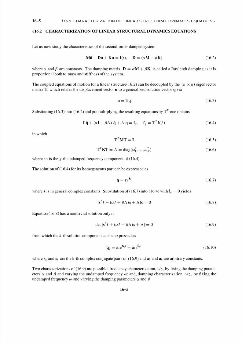
Let us now study the characteristics of the second-order damped system

M¨u

+D

˙u

+Ku

=f (t ), D

=(αM

+βK) (16.2)

where α and β are constants. The damping matrix, D = αM + βK, is called a Rayleigh damping as it is

proportional both to mass and stiffness of the system.

The coupled equations of motion for a linear structure(16.2) can be decoupled by the (n × n) eigenvector

matrix T, which relates the displacement vector u to a generalized solution vector q via

u = Tq (16.3)

Substituting (16.3) into (16.2) and premultiplying the resulting equations by TT one obtains

I q + (αI + β) q + q = f q , f q = TT f ( f ) (16.4)

in which

TT MT = I (16.5)

TT KT = = diag(ω21,...,ω2

N ) (16.6)

where ω j is the j -th undamped frequency component of (16.4).

The solution of (16.4) for its homegeneous part can be expressed as

q = cest

(16.7)

where s is in general complex constants. Substitution of (16.7) into (16.4) with f q = 0 yields

{s2 I + (α I + β)s + }c = 0 (16.8)

Equation (16.8) has a nontrivial solution only if

det |s2 I + (α I + β)s + | = 0 (16.9)

from which the k -th solution component can be expressed as

qk = ak esk t + ak e

sk t (16.10)

where sk and sk are the k-th complex conjugate pairs of (16.9) and ak and ak are arbitrary constants.

Two characterizations of (16.9) are possible: frequency characterization, viz., by fixing the damping param-

eters α and β and varying the undamped frequency ω; and, damping characterization, viz., by fixing the

undamped frequency ω and varying the damping parameters α and β .

16–5




-8 -7 -6 -5 -4 -3 -2 -1 0 1-4

-3

-2

-1

0

1

2

3

4Root loci of proportionally damped structural dynamics equation

Real part of normalized frequency by sampling rate h

I m a g i n a r y p a r t o f n o r m a l i z e d f r e q u e n c y b y s a m p l i n g r a t e h

o 0

Increasing frequency

Increasing frequency

s1 s

2A

B

o

B

C

− −( 1− α β )1/2 ____________

β−

−(−1/β, 0)

Fig. 5.1 Root Loci of Proportionally Damped Structural Dynamics System

§16.2.1 Frequency Characterization Based on the Root Locus Method

The characteristic equation (16.9) represents n roots:

s2 j + (α + βω2

j )s j + ω2 j = 0, j = {1, 2, . . . , n} (16.11)

Since not only the distribution but also the maximum and minimum frequencies are not known a-priori, a

complete range of the Rayleigh-damped system can be characterized by the following expression:

s2 + (α + βω2)s + ω2 = 0 0 ≤ ω ≤ ∞ (16.12)

In order for the subsequent characterization to remain valid for all sampling rates, we normalize (16.12) by

the sampling rate h such that

¯s2

+(αh

+β

h(ωh)2)

¯s

+(ωh)2

=0 0

≤ωh

≤ ∞⇓

s2 + (α + βω2)s + ω2 = 0, α = αh, β = β

h, ω = ωh

(16.13)

Note first that the rigid-body motion (i.e., ω = ωh = 0) corresponds from (16.13) to:

s1 = {0, 0} and s2 = {−αh, 0} = { −α, 0} (16.14)

16–6



16–7 §16.2 CHARACTERIZATION OF LINEAR STRUCTURAL DYNAMICS EQUATIONS

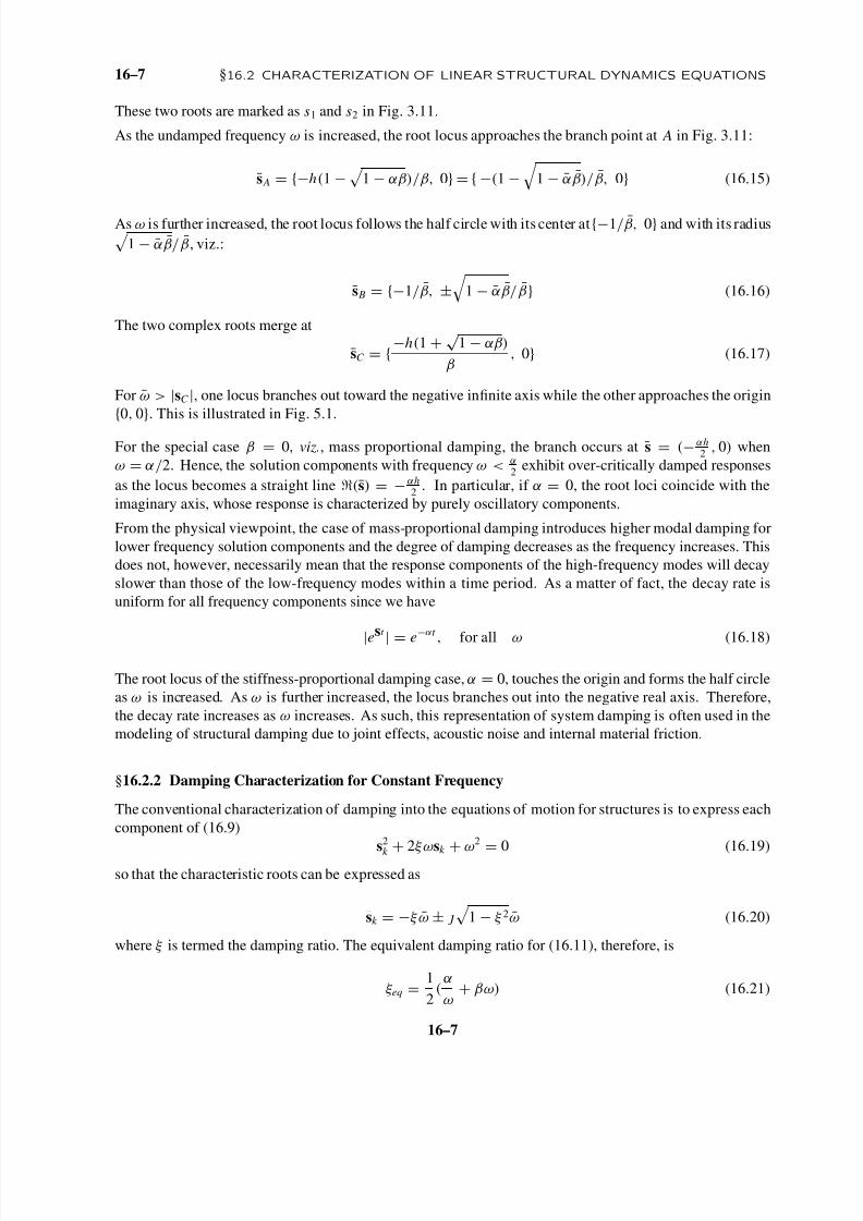
These two roots are marked as s1 and s2 in Fig. 3.11.

As the undamped frequency ω is increased, the root locus approaches the branch point at A in Fig. 3.11:

s A = {−h(1 −

1 − αβ)/β, 0} = { −(1 −

1 − αβ)/β, 0} (16.15)

As ω is further increased, the root locus follows the half circle with its center at {−1/β, 0} and with its radius 1 − αβ/β, viz.:

s B = {−1/β, ±

1 − αβ/β} (16.16)

The two complex roots merge at

sC = {−h(1 + √ 1 − αβ)

β, 0} (16.17)

For ω > |sC |, one locus branches out toward the negative infinite axis while the other approaches the origin

{0, 0

}. This is illustrated in Fig. 5.1.

For the special case β = 0, viz., mass proportional damping, the branch occurs at s = (− αh2

, 0) when

ω = α/2. Hence, the solution components with frequency ω < α2

exhibit over-critically damped responses

as the locus becomes a straight line (s) = − αh2

. In particular, if α = 0, the root loci coincide with the

imaginary axis, whose response is characterized by purely oscillatory components.

From the physical viewpoint, the case of mass-proportional damping introduces higher modal damping for

lower frequency solution components and the degree of damping decreases as the frequency increases. This

does not, however, necessarily mean that the response components of the high-frequency modes will decay

slower than those of the low-frequency modes within a time period. As a matter of fact, the decay rate is

uniform for all frequency components since we have

|est

| = e−αt

, for all ω (16.18)

The root locus of the stiffness-proportional damping case, α = 0, touches the origin and forms the half circle

as ω is increased. As ω is further increased, the locus branches out into the negative real axis. Therefore,

the decay rate increases as ω increases. As such, this representation of system damping is often used in the

modeling of structural damping due to joint effects, acoustic noise and internal material friction.

§16.2.2 Damping Characterization for Constant Frequency

The conventional characterization of damping into the equations of motion for structures is to express each

component of (16.9)

s2

k +2ξ ωsk

+ω2

=0 (16.19)

so that the characteristic roots can be expressed as

sk = −ξ ω ±

1 − ξ 2ω (16.20)

where ξ is termed the damping ratio. The equivalent damping ratio for (16.11), therefore, is

ξ eq =1

2(

α

ω+ βω) (16.21)

16–7




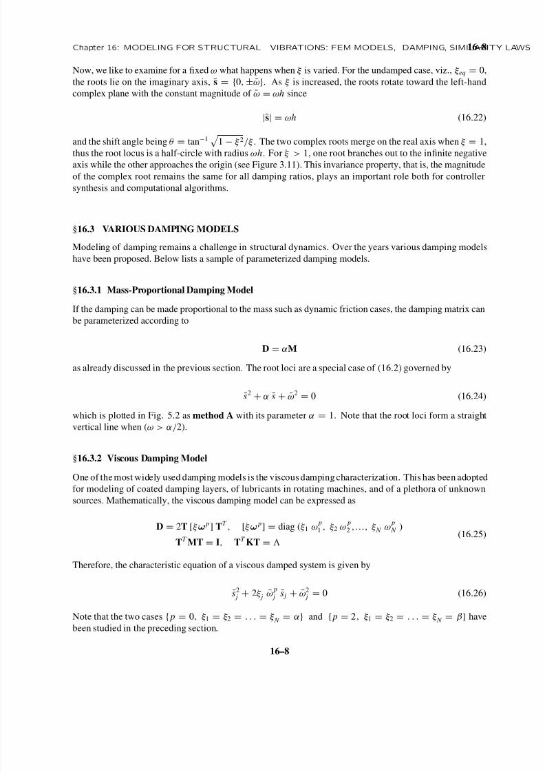
Now, we like to examine for a fixed ω what happens when ξ is varied. For the undamped case, viz., ξ eq = 0,

the roots lie on the imaginary axis, s = {0, ±ω}. As ξ is increased, the roots rotate toward the left-hand

complex plane with the constant magnitude of ω = ωh since

|s| = ωh (16.22)

and the shift angle being θ = tan−1

1 − ξ 2/ξ . The two complex roots merge on the real axis when ξ = 1,

thus the root locus is a half-circle with radius ωh. For ξ > 1, one root branches out to the infinite negative

axis while the other approaches the origin (see Figure 3.11). This invariance property, that is, the magnitude

of the complex root remains the same for all damping ratios, plays an important role both for controller

synthesis and computational algorithms.

§16.3 VARIOUS DAMPING MODELS

Modeling of damping remains a challenge in structural dynamics. Over the years various damping models

have been proposed. Below lists a sample of parameterized damping models.

§16.3.1 Mass-Proportional Damping Model

If the damping can be made proportional to the mass such as dynamic friction cases, the damping matrix can

be parameterized according to

D = αM (16.23)

as already discussed in the previous section. The root loci are a special case of (16.2) governed by

¯s2

+α

¯s

+ ¯ω2

=0 (16.24)

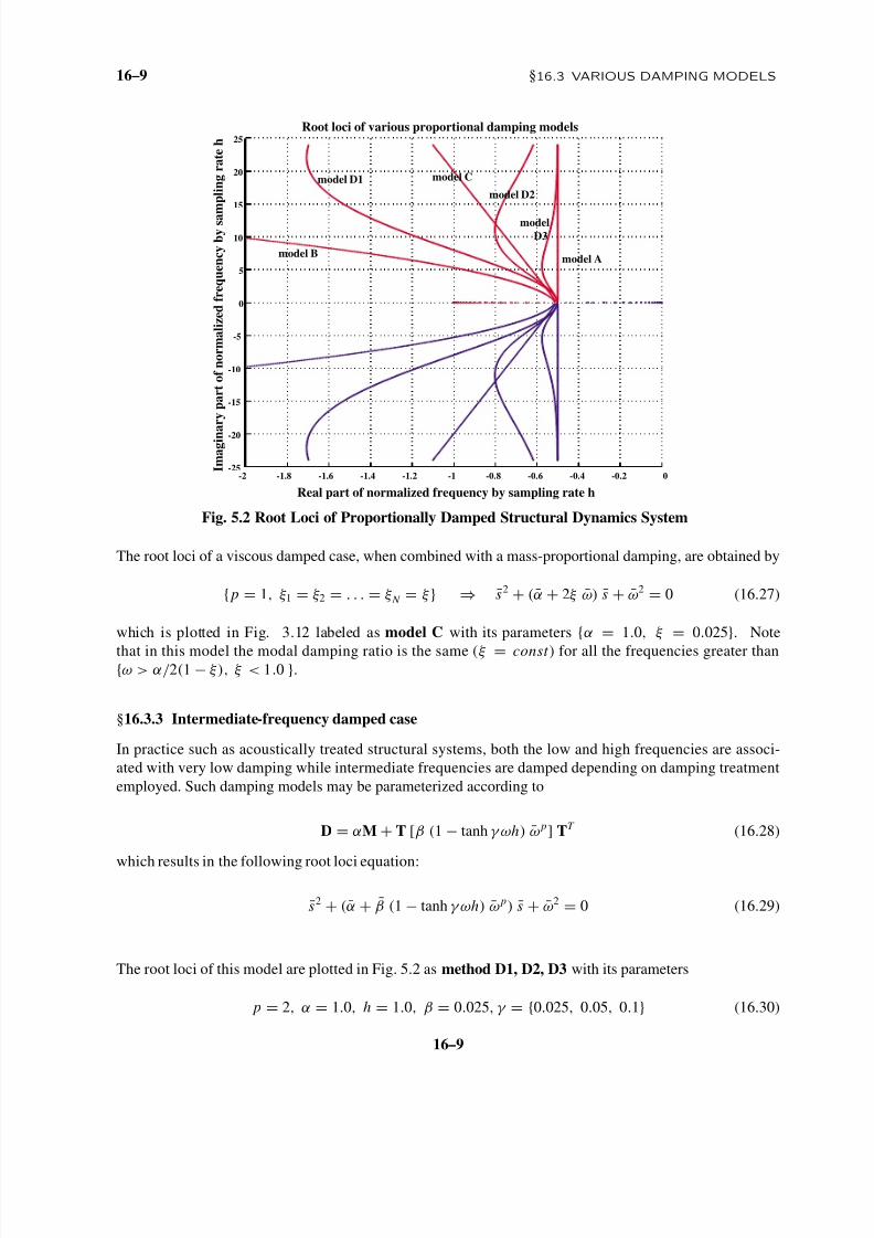
which is plotted in Fig. 5.2 as method A with its parameter α = 1. Note that the root loci form a straight

vertical line when (ω > α/2).

§16.3.2 Viscous Damping Model

One of the most widely used damping models is the viscous damping characterization. This has been adopted

for modeling of coated damping layers, of lubricants in rotating machines, and of a plethora of unknown

sources. Mathematically, the viscous damping model can be expressed as

D = 2T [ξ ω p] TT , [ξ ω p] = diag (ξ 1 ω p

1 , ξ 2 ω p

2 ,..., ξ N ω p

N )

TT MT = I, TT KT = (16.25)

Therefore, the characteristic equation of a viscous damped system is given by

s2 j + 2ξ j ω p

j s j + ω2 j = 0 (16.26)

Note that the two cases { p = 0, ξ 1 = ξ 2 = . . . = ξ N = α} and { p = 2, ξ 1 = ξ 2 = . . . = ξ N = β} have

been studied in the preceding section.

16–8



16–9 §16.3 VARIOUS DAMPING MODELS

-2 -1.8 -1.6 -1.4 -1.2 -1 -0.8 -0.6 -0.4 -0.2 0-25

-20

-15

-10

-5

0

5

10

15

20

25

Root loci of various proportional damping models

Real part of normalized frequency by sampling rate h

I m a g i n a r y p a r t o f n o r m a l i z e d f r e q u e n c y b y s a

m p l i n g r a t e h

model Amodel B

model Cmodel D1

model D2

model

D3

Fig. 5.2 Root Loci of Proportionally Damped Structural Dynamics System

The root loci of a viscous damped case, when combined with a mass-proportional damping, are obtained by

{ p = 1, ξ 1 = ξ 2 = . . . = ξ N = ξ } ⇒ s2 + (α + 2ξ ω) s + ω2 = 0 (16.27)

which is plotted in Fig. 3.12 labeled as model C with its parameters

{α

= 1.0, ξ

= 0.025

}. Note

that in this model the modal damping ratio is the same (ξ = const ) for all the frequencies greater than{ω > α/2(1 − ξ ), ξ < 1.0 }.

§16.3.3 Intermediate-frequency damped case

In practice such as acoustically treated structural systems, both the low and high frequencies are associ-

ated with very low damping while intermediate frequencies are damped depending on damping treatment

employed. Such damping models may be parameterized according to

D = αM + T [β (1 − tanh γ ωh) ω p] TT (16.28)

which results in the following root loci equation:

s2 + (α + β (1 − tanh γ ωh) ω p) s + ω2 = 0 (16.29)

The root loci of this model are plotted in Fig. 5.2 as method D1, D2, D3 with its parameters

p = 2, α = 1.0, h = 1.0, β = 0.025, γ = {0.025, 0.05, 0.1} (16.30)

16–9




Note that as ω becomes large, the real part of the root loci approaches

s → −α as ω → ∞ (16.31)

Hence, if α = 0 the root loci will lie on the imaginary axis, indicating no damping for those frequencies.

§16.4 USE OF SIMILARITY LAWS IN MODELING

Dimensional analysis has been widely used in experiment design and scale-model construction. The task

in dimensional analysis is to identify physical quantities that influence the physical phenomena on hand,

then deduce a independent set of dimensionless products. These dimensionless products are then utilized for

experiment design and scale-model construction. The underlying principle is Buckingham’s theorem that

enables a systematic construction of linearly independent dimensionless products. It should be pointed out

that dimensional analysis is applicable both to statics and dynamics. In dynamics, a useful ‘dimensional’

analysis may be carried out, which can provide insight into dynamic behavior. It is referred to mechanical

similarity after Landau and Lifshits. The basic idea is as follow.

The starting point of mechanical similarity is that multiplication of kinetic and potential energy expression

or the Lagrangian by any constant does not affect the equations of motion. It is this observation that can

yield the dynamic behavior of a system without actually solving the equations of motion.

For example, we may pose the question: Does the amplitude of string vibration affect the frequency, assuming

its potential energy is a quadratic function of its amplitudes? To answer this question, let us consider the

simplest case, i.e., a single mass and a single spring case given by

T = 12

m ˙ x 2, U = 12

k x 2 ⇒ L = T − Y

⇓m ¨ x + k x = 0, x (0) = x 0, ˙ x (0) = ˙ x0

(16.32)

where m and k are the mass and spring constant, x is the vibration amplitude, and x0 and ˙ x0 are the initial

amplitude and velocity of the mass.

Of course, we all know that the frequency of the above system is given by

ω =

k /m (16.33)

which clearly shows that the frequency ω is independent of the amplitude x (t ).

Let us scale the new amplitude x by

χ = x

x(16.34)

so that the potential energy U changes to

U ( x ) = 12

k ( x )2 = 12

χ 2 x 2 (16.35)

Now we introduce the time scale

τ = t

t (16.36)

where τ characterizes the ratio of periods of motion or time durations of the two systems.

16–10



16–11 §16.4 USE OF SIMILARITY LAWS IN MODELING

The kinetic energy fo the system is now changed to

K ( x , t ) = 12

m(d x

∂ t )2 = 1

2(

χ

τ )2 m ˙ x 2 (16.37)

Therefore, the Lagrangian of the new system becomes

L = T − U = 1

2(

χ

τ )2 m ˙ x 2 − 1

2χ 2 x 2 = χ 2 (

1

τ 2 · 1

2m ˙ x 2 − 1

2k x 2) (16.38)

The above equation states that the only way the resulting equation of mition is unaltered is to choose

τ = t

t = 1

⇓L

= χ 2 ( 12

m ˙ x 2 − 12

kx 2) = χ 2L

(16.39)

Since the time scale ratio is unity, it means that the frequencies for both systems are the same. In other words,

the frequencies of a lumped spring-mass system is unaffected by their vibration amplitudes.Comparing (16.33) and (16.39) one may argue that the mechanical similarity method is somewhat more

complicated than what could be obtained by the frequency equation (16.33). Its chief advantage is that one

needs not solve the governing equation (16.32) for its frequency expression.

Kepler’s Third Law: Let us now apply the mechanical similarity to the motions of two satellites around a

heavenly body. Newton’s law of universal gravitation states

F = G Mm

r 2 ⇒ U = − G Mm

r (16.40)

where G is the universal gravitational constant, M and m are the masses of the heavenly body and the satellite,

and r is the distance between the two bodies. The Lagrangian of the two satellites may be expressed as

L1 = 12

m1v1 · v1 + G Mm1

|r1|, v1 =

d r1

dt 1

L2 = 12

m2v2 · v2 + G Mm2

|r2|, v2 =

d r2

dt 2

(16.41)

Let us transform L2 by introducing

t 2 = τ t 1, r2 = χr1 (16.42)

to obtain

L2 = c( 12

m1v1 · v1 + τ 2

χ 3 · G Mm1

r 1), c = m2

m1

· (χ

τ )2 (16.43)

Note that the above scaling on L2 amounts to a thought experiment in which the satellite m 2 is brought tothe orbit of satellite m 1. For this thought experiment to be true, its corresponding equation of motion should

be the same as that obtained by L1. This can be the case only if the following condition is satisfied:

L2 = c L1 ⇒ τ 2

χ 3 = 1 ⇒ (

t 2

t 1)2 = (

r 2

r 1)3 (16.44)

which states that square of the revolution ratio of the two satellites is proportional to the cube of the ratio of

the orbital sizes, Kepler’s third law.

16–11




The Race between a Sliding Block and a Rolling Cylinder on an Inclined Slope Consider a cube sliding

on an inclined plane without friction, whose Lagrangian can be expressed as

Lcube = 12ms2 − mgs sin θ (16.45)

where m is the mass of the cube, s is the distance along the slope measured from the bottom of the slope, g

is the gravity, θ is the inclined angle of the slope, and s is the speed of the cube along the slope.

If a cylinder of the same mass m is to roll along the slope without slip, its Lagrangian can be obtained as

Lcyl = 12m(s)2 + 1

2( 1

2mr 2)ω2 − mgs sin θ (16.46)

where r is the radius of the cylinder, and ω is the angular velocity of the cylinder during rolling without slip.

Since the angular velocity can be expressed in terms of s as

ω = s

r , s = ∂s

∂t (16.47)

(16.46) can be simplified to

Lcyl = 12

3m

2 (s)2 − mgs sin θ (16.48)

Transforming the above by the scaling

t /t = τ, s/s = χ (16.49)

yields

Lcyl = 12

3m

2

χ 2

τ 2 (s)2 − mgsχ sin θ = 3

2

χ 2

τ 2 [ 1

2ms2 − 2τ 2

3α· mgs sin θ ] (16.50)

Comparing the above with (16.45), we find for the resulting equation of motion from (16.50) to be the same

as obtained by (16.45) we must have

2τ 2

3χ= 1 ⇒ τ = t

t =

3χ2

(16.51)

Now if the distance is the same, i.e., s = s, we have χ = 1. Therefore, the cylinder will arrive at the bottom

of the inclined slope by a factor of

32

longer over the arrival time of the cube.

In other words, the cube will arrive at the bottom faster than the cylinder, and the arrival time ratio of the

two bodies will be proportional to the ratio of the square root of the kinetic energies. Physically, the reason

for the slower average speed of the cylinder is because for the case of cylinder, the same potential energy

change is translated into both the translational and rotational kinetic energy while the entire change energy

gets into the translational kinetic energy for the cube.

§16.4.1 Mechanical Similarity in String, Rod and Shaft Vibrations

The Lagrangian of strings, rods and shafts can be expressed as

L = T − U

T = 12

0

m( x) [∂w( x, t )

∂ t ]2 dx

U = 12

0

k ( x) [∂w( x, t )

∂ x]2 dx

(16.52)

16–12



16–13 §16.4 USE OF SIMILARITY LAWS IN MODELING

where m( x) is the mass per unit length for string and rods, and the mass moment of inertia for shafts,

respectively; and k ( x) denotes the tension force, the product of Young’s modulus and the cross section area

E A( x), and the shear rigidity G I ( x) for strings, rods and shafts, respectively.

Let us consider the following scaling transformations:

m m

= µ k k

= κ, x x

= χ =

, t t

= τ = p p

(16.53)

which, when substituted into (16.52), yields

L = (

µχ

τ 2 ) T − (

κ

χ) U = (

µχ

τ 2 ) · [T − (

κτ 2

µχ 2) U ] (16.54)

In order for the transformations not to affect the resulting equations of motion, we must have

L

L= C E = (

µχ

τ 2 ) ⇒ κτ 2

µχ 2 = 1 ⇒ τ =

µ

κ· χ

⇓

Period ratio = p

p= k /m

k /m ·

(16.55)

where C E is the energy ratio whose role we will discuss shortly.

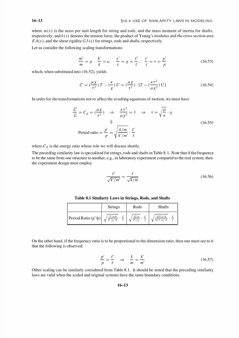
The preceding similarity law is specialized for strings, rods and shafts in Table 8.1. Note that if the frequency

to be the same from one structure to another, e.g., in laboratory experiment compared to the real system, then

the experiment design must employ

√ k /m =

√ k /m (16.56)

Table 8.1 Similarty Laws in Strings, Rods, and Shafts

Strings Rods Shafts

Period Ratio (p’ /p)

T /ρ A

T /ρ A ·

E /ρ

E /ρ ·

GI /ρ A

G I /ρ A ·

On the other hand, if the frequency ratio is to be proportional to the dimension ratio, then one must see to it

that the following is observed:

p

p=

⇒ k

m= k

m (16.57)

Other scaling can be similarly considered from Table 8.1. It should be noted that the preceding similarity

laws are valid when the scaled and original systems have the same boundary conditions.

16–13




Observe that the similarity laws summarized in Table 8.1 can be derived if one solves for each of the three

vibration problems. The emphasis is to utilize the respective energy expressions rather than the solutions

of the governing differential equations. This is because it is often considerably easier to obtain the energy

expressions of a system than obtain the vibration characteristics or quasi-static deformations.

Finally, let us consider the role of the energy ratio

C E = ( µχτ 2

) (16.58)

which plays a pivotal role in sizing up the experiment design as it offers the experiment energy requirements

relative to the actual system. In practice it is often the energy requirement that dictates the scaling than the

geometrical considerations. Notice that since we have only one constraint for four parameters, the remaining

three parameters can be used in meeting practical considerations in experiment design.

§16.4.2 Mechanical Similarity in Euler-Bernoulli Beam

The Lagrangian of a continuous Euler-Bernoulli beam can be expressed as

L

= T

−(U m

+U g)

T = 12

0

ρ A( x) [∂w( x, t )

∂ t ]2 dx

U m = 12

0

E I ( x) [∂2w( x, t )

∂ x2 ]2dx

U g = 12

0

P( x) [∂w( x, t )

∂ x]2 dx

(16.59)

where w( x, t ) is the transverse displacement of the neutral axis of the beam, m( x) is the mass per unit beam

length, E I ( x) denotes the bending rigidity of the beam, and P( x) denotes the pre-stressed axial force.

Introducing the scaling transformations given by (16.53) as modified to the case of beam, the Lagrangian of

the new system can be expressed as

L = (

µχ

τ 2 ) T − κ

χ 3U m − f

χU g, κ = E I

E I , f = P

P

= (µχ

τ 2 ) [T − (

κτ 2

µχ 4) [U m + (

f χ 2

κ) U g]

⇓

L = (

µχ

τ 2 ) L, if (

κτ 2

µχ 4) = 1 and (

f χ 2

κ) = 1

(16.60)

Therefore, the similarity law for a beam is expressed as

p

p=

E I /ρ A

E I /ρ A · (

)2 provided

P ( x)

P( x)= E I

E I · 2

2, if P( x) = 0 (16.61)

Notice that the appendage arms for a spinning satellite, helicopter rotor blades and turbine blades all experi-

ence axial tensions. Hence, the scaling of beam sizes must consider the axial force scaling as well.

One important application of the preceding scaling law is for the experiment design of rotating members for

micro-machine members as the rotating speed is very high and experiment design often necessitates a scaling

up rather than scaling down.

16–14

strucutural vibrations

Documents