1

TABLE OF CONTENT

INTRODUCTION I.1.

1.1. Construction 1.1. I. SYNCHRONOUS MACHINE 1.1.

1.2. Constructive types 1.4.

2.1. Voltage equations in phase quantities 2.2. II. TRANSIENT REGIME 2.1.

2.2. Inductances 2.3. 2.3. PARK’s transformation 2.4. 2.4. Flux expressions 2.6. 2.5. Electromagnetic torque 2.7. 2.6. Referred and base quantities 2.7. 2.7. Per-unit quantities 2.9. 2.8. Voltage and flux equations in per-unit 2.10. 2.9. Motion equation in per-unit 2.11. 2.10. Graphical representation of the fluxes 2.12. 2.11. Equivalent diagrams 2.13. 2.12. Time constants and reactances 2.14. 2.13. Synchronous machine’s operational reactances 2.16. Steady state regime – particular case: reactive synchronous machine 2.17. Examples 2.19.

3.1. Present situation of the research 3.1. III. ANALYTICAL IDENTIFICATION OF THE PARAMETERS 3.1.

3.2. Analytical identification 3.3. 3.2.1. Stator’s parameters 3.3.

a). Leakage inductance 3.3. a1). Slot leakage inductance 3.3. a2). End-winding leakage inductance 3.5.

b). magnetization inductance 3.6. b1). Stator winding factor 3.7. b2). Carter’s factor. Equivalent air-gap 3.8.

c).stator resistance 3.8. 3.2.2. Rotor’s parameters 3.8.

a). excitation winding parameters 3.9. a1). Leakage inductance 3.9. a2). Effective inductance 3.10. a3). Resistance 3.12.

b). Damping-cage parameters 3.13. b1). Self-inductances 3.13. b2). Leakage inductances 3.15. b3). Resistance 3.16.

c). Stator winding reference 3.16. 3.2.3. Example for caged synchronous machine steady state regime 3.21.

a). damper bar current calculation considering each loop

2

as independent circuit 3.22. b). damper bar current calculation considering a sinusoidal

distribution in loops 3.25. 3.2.3. Stator and excitation winding effective inductance calculation 3.27.

a). Permeance distribution curve 3.27. b). Leakage inductance calculation 3.28.

3.2.5. Example of analytical calculation method for VRSM 3.32. Examples 3.34.

4.1. Classical methods 4.1. IV. EXPERIMENTAL IDENTIFICATION OF THE PARAMETERS 4.1.

4.1.1. Subtransient reactance from static method 4.1. 4.1.2. Synchronous reactance from slip test 4.2. 4.1.3. Reactances from L.C. Mamiconiants method 4.4. 4.1.4. xd, xq for cageless VRSM 4.5.

4.2. Reactances determination from functioning curves 4.6. 4.2.1. No-load measurement 4.6. 4.2.2. Steady-state, 3-phase sudden short-circuit 4.6. 4.2.3. Load test 4.7.

4.3. 3-phase symmetrical sudden short-circuit 4.9. 4.4. Standstill frequency response tests 4.13.

4.4.1. d-axis 4.13. 4.4.2. q-axis 4.16.

5.1. d- or q-axis for fixed rotor position 5.1. V. PARAMETERS’ IDENTIFICATION FROM STANDSTILL DC DECAY TEST 5.1.

5.1.1. Theory elements regarding current identification 5.1. 5.1.2. Current identification using m.e.f. 5.6. 5.1.3. DC decay test simulated on a 2D-FEM modeled generator 5.8.

5.2. Random position of the rotor 5.12. 5.2.1. General case 5.12. 5.2.2. Particular case 5.19. 5.2.3. Determination of rotor’s position 5.27.

5.3. Measurements equipment 5.30. 5.4. Simulations 5.32.

5.4.1. Identification program 5.32. a). Procedure validation 5.33. b). SIMSEN presentation 5.34.

5.5. Results 5.35. 5.5.1. Identification procedure for d- and q- axis 5.35. 5.5.2. General case - random rotor position 5.41.

VI. CONCLUSIONS AND CONTRIBUTIONS C.1.

GLOSSARY L.1. BIBLIOGRAPHY B.1. APPENDICES A.1.

3

INTRODUCTION

The synchronous generators, with a large power unit, are producing most of the electric energy in need all over the world. Since the synchronous machine model is based on its parameters, the need for a reliable set of electrical parameters is obvious. The parameters can be calculated analytically or via a magnetic field analysis procedure during the design stage of the machine. The parameters can be obtained also by tests at the factory or on site. The magnetic field analysis technique, usually via a 2D or 3D-finite element method (FEM), for instance, offers good results in calculating the machine parameters, proving its versatility and high accuracy too. As far as the test determination of the synchronous machine is concerned two are the most used up to now, the standstill frequency response (SSFR) and the short circuit. The standstill frequency response (SSFR) test has become a common method of determining the machine parameters, I.M. Canay being one of the important contributors in this domain. A quite classic test used to calculate the synchronous machine parameters is short-circuit one even it weakness consists mostly in less adequately treating the case of higher order models. The time-domain identification of the synchronous machine parameters based on DC decay test is quite a new procedure and its main lack is the identification of the parameters for a random position of the rotor. New interesting approaches are presented but only for the two fixed axis (d- and q-) and with a real need of good estimation for the initial parameters. In the same time, the DC decay test is simple, without any risk and less expensive. The DC decay test allows for determination of the machine’s parameters only through an identification procedure, being, as is short-circuit test too, a time-domain test.

Usually, the characteristic values of a synchronous machine are obtained from a short-circuit test at no-load. This test requires substantial equipment and is therefore expensive, it implies risks and it cannot be always carried out for levels of voltage higher than 50% to 60% of nominal voltage. The DC decay test is an interesting alternative since only light equipment is needed. It delivers the characteristic values of synchronous machine for the two axes in function of the saturation state of the leakage paths. In general, the DC decay test is done for the two extreme positions of the rotor, d- and q- axes. This contribution proposes a solution for a DC decay test extended for a random position of the rotor. The extension is important because, at standstill, it is almost impossible to fix the rotor of a large synchronous machine in a particular position.

The thesis has 6 chapters. Chapter I presents the synchronous machine:

construction, types, etc. In the second chapter the transient regime of synchronous machine from the theoretical point is given. This includes Park’s transformations, equivalent circuits, reactances, inductances, time constants. Also, there are the equations of transient regime for a synchronous reactive machine. Finally, same examples are found: asynchronous operation, electromechanical oscillations, sudden short-circuit.

4

The third part is dedicated to analytical identification of the parameters, including the present situation of the research, a model of a caged synchronous machine and some examples of computations. In chapter IV are presented experimental methods of the parameters, classical tests (slip test, Mamiconiants, etc.) and new approaches (standstill frequency response, steady-state short-circuit, etc).

In chapter V standstill DC decay test is presented. A method of parameters identification is given, for a fixed rotor position, in d- and q axis, and also, o new method for a random position. There are the obtained results, too.

Finally, conclusions and contributions, glossary, bibliography and appendices are found.

III. ANALYTICAL IDENTIFICATION OF THE PARAMETERS

Obtaining of parameters of a synchronous machine is and will be an important step of the

designing procedure, and the study of the machine transient is also requiring a good estimation of the parameters. An appropriate determination allows knowing precisely the machine behaviour in different operating regimes.

There are many proposed methods to obtain the parameters from tests, identification and estimating methods, while the analytical approaches are lately neglected; it is one of the reasons why this paper tries to prove that some analytical approaches can give satisfactory results depending on the considered assumptions.

The most important aspect in computing the damper winding is to obtain the current distribution in each damper bar. One approach to obtain the damper bar currents would be to consider a sinusoidal damper bar current distribution in respect with d- and q-axis. This assumption where a set of equations were obtained gave satisfactory results compared with the test based results. A more precise solution would be to take each damper bar as a separate rotor circuit or to group the bars in loops and consider the mutual coupling between loops and between the loops and the other windings of the machine.

For grouping the bars in loops, two solutions were identified: 1 – A loop will consist from two bars, symmetrically positioned in respect with the pole magnetic symmetry axis, and a part from the short circuit ring between these bars. 2 – The second solution would be to replace the damper winding with a two-phase equivalent winding. The equivalence should be made on bars or on loops; a loop consisting in this case from two adjacent bars and the end ring between these bars. In this case all the resistances and inductances would be identical.

Two analytical methods for calculating the parameters and the damper bar currents are presented. Both of them are based on grouping two symmetrically located bars into loops. The first method will consider each loop as an independent rotor circuit, having a resistance, a self and mutual inductance (considering the coupling with the stator, with the field winding – on d-axis, and with the other loops). Considering this, in the system of voltage and flux equations of the synchronous machine will be introduced for the damper winding as many equations as bars are on one pole.

5

In the second method discussed here, a sinusoidal distribution of currents in the damper winding is assumed. An equivalent current and voltage is defined and the damper winding will be reduced to an equivalent winding on both axes, with an equivalent resistance and inductance. The rotor parameters will be referred to the stator side.

a). Calculating the damper bar current by considering each loop as independent circuit In order to obtain the damper bar current distributions, first all the parameters must be

known. The number of parameters that must be calculated depends on the number of pole bars. The air gap flux given analytically has the following expression:

∫∫ ⋅⋅= dxdlBφ (3.124)

xRii

xx dx

dIlN

ldxdB λφ

⋅⋅== (3.125)

where N is the number of turns per pole of a given rotor circuit, li is the machine ideal length and IR is the current from a rotor circuit (filed winding or a loop). The permeance associated for an elemental length (dx) of the pole pitch:

dxlddi

ix δ

µλλλ

λλλ ⋅⋅=⋅= 0

00

0

(3.126)

The ratio λ/λ0 was introduced because the permeance distribution through the air gap is not constant and is given in 3.2.4.

The self and mutual inductances must be calculated separately for each rotor circuit. First, few relations will be presented in order to obtain the field winding self and mutual inductances. The field winding self inductance is composed by two terms; the main magnetizing inductance (LhF) and the leakage inductance (LσF):

FhFF LLL σ+= (3.127) The flux produced by a pole, if only the field winding is fed, comes as:

20

2p

hF p i xl B dxτ

τΦ = ⋅ ⋅ ⋅ ∫ (3.128)

The total flux produced by the field winding:

FhFhFFhF ILN ⋅=⋅=Ψ φ (3.129) Where the magnetizing inductance is:

hFFhF CNL ⋅⋅= 2λ (3.130)

with λ and ChF given in (3.57) and (3.45).

The damper winding inductances must be calculated for each loop and for both d- and q-axis. The flux produced on d-axis by the nth loop:

nnDnDDnnD CIN ⋅⋅⋅= λφ (3.133)

while the total flux produced by all nth loops from all poles is

nnDnDDnnD CIN ⋅⋅⋅=Ψ λ2 (3.134)

6

where ND=2p and represents the total number of n degree loops for the whole machine and InD is the current flowing through loop n. The direct axis nth loop main inductance came as:

nnDDnnD CNL ⋅⋅= 2λ (3.135)

∫ ⋅⋅⋅

= 20

0

2

4

nn

dxCp

nnD

τ

λλ

τπ (3.136)

The q-axis damper loops magnetizing inductances can be calculated similarly with the ones from the d-axis. In this case the functions f1 and f2, which are defining the permeance curve, will have the (3.67) expressions.

In the case of a damper winding with an odd number of bars per pole, the q-axis will have one loop more than the d-axis because of the central bar.

The calculated leakage inductance of the loops is based on the specific permeance method. For a circular slot (the section of bars is circular) the specific permeance λb is independent of slot diameter and is equal to 0.62. To this value, the slot opening and the tooth top leakage should be added as the damper ring leakage is added too (this has a small value and can be neglected).

The mutual effect between the damper and field winding exists only on the d-axis. Thus, we will have a mutual field-loop inductance for each single turn damper winding.

nnFDFnnF CNNL ⋅⋅⋅= λ (3.139) where CnnF is equal to CnnD .

Another type of coupling can be considered the coupling between loops. This mutual effect yields to another set of parameters.

ijDDjDiijD CNNL ⋅⋅⋅= λ (3.142)

the common flux is considered as mutual, than:

ijDijD CC min= (3.143)

The resistances of the different loops are calculated from the machine designing dimensions considering the damper ring and the skin effect at starting. To facilitate the calculation a per-unit system has to be adopted. A reference system for each rotor circuit with base values for currents, voltages and impedances [8] is defined. It was assumed that each loop is going to be a separate circuit. Thus, for a pole with n bars, a system with n+3 equations and n+3 unknown quantities (the damper currents) will be obtained at a given slip, since the angle Θ is a function of slip and angular frequency,

0)1( Θ+⋅⋅−=Θ ts ω (3.144) b). Calculating the damper bar currents by considering a sinusoidal distribution in loops

The second method of analytical calculation, presented in this paper, reduces the damper winding to two equivalent windings, one with its magnetic axis in line with the direct- and one with the quadrature axis. The method is applicable when the damper windings have the bars with the same chemical composition and cross section. The flux density has a pulsating

7

sinusoidal distribution in space with its magnetic axis in the pole axis. The currents induce in each pair of bars located at the same distance from the pole axis will have the same magnitude and an opposite flowing direction.

The previous definition of a loop (Fig.3.8, 3.9) remains valid in this situation too; but instead of treating each loop separately, will be assumed that the currents with the maximum magnitude are induced in the loop that would be located at a half pole pitch from the flux wave axis [T1].

The currents from each loop positioned at the electric angle θ/2 from the flux wave axis will have a magnitude equal to sin (θ/2) from the maximum magnitude.

An important simplifying assumption introduced in this approach is that the mmf produced by any loop has a rectangular distribution. This assumption is not entirely true at a machine with salient poles and a variable air gap along the pole tip, but only in this way the damper winding can be reduced to an equivalent one circuit winding. Thus, the magnitude of the fundamental direct axis MMF component corresponding to the nth loop will be:

⋅=

2sin4

maxn

nDnd IF θπ

(3.146)

and the resultant space fundamental mmf of all the loops is:

∑=

⋅=

DdN

k

kDdDd IF

1

2

2sin4 θ

π (3.147)

where NDd is the number of loops. Considering this, for both odd and even number of bars per pole, the resultant space

fundamental mmf on d-axis can be expressed as:

( )bDdbDd kInF −⋅⋅⋅= 11π

(3.148)

)sin()sin(1

bb

bbb n

nkαα

⋅⋅

−= (3.149)

The expressions of the referred parameters are [T1]: - the equivalent damper winding leakage inductance referred to the stator, with Ldσ

being the equivalent single bar direct axis leakage:

( ) σσ dbb

wSSrD L

knpkNL ⋅−⋅⋅

⋅⋅=

1)(8 2

(3.152)

- the mutual inductance between the stator phase and the equivalent damper winding referred to stator:

adwSS

SDr CpkNL ⋅⋅⋅

= λ2)( (3.153)

- the referred stator-field, field-equivalent damper winding and stator-direct axis equivalent damper winding mutual inductances have the same value.

FDrSFrSDr LLL == (3.155) - the equivalent damper winding resistance referred to stator (3.93)

8

- the referred field winding leakage inductance and resistance (3.104) and (3.105) Also the ration between the actual and referred field currents is:

F

wSS

hF

ad

Fr

F

NpkN

CC

II

⋅⋅

⋅⋅=π4

(3.156)

Example 2: The sample machine considered as example is a three phase one with rated power of 7.5

MVA, two pole pairs and 9 bars per poles. After obtaining all the machine parameters with both methods, the obtained voltage systems, with 12 respectively with 5 voltage equations, were solved for a given slip (s=1) and voltage (u=0.186 p.u. corresponding to

VU 310656.12 ⋅= rated phase voltage). The considered operating regime was an asynchronous starting with short-circuited field winding. In Table 1, the actual values of damper bar currents are presented, obtained with the above presented methods and the currents obtained with a numerical approach [S6].

Table3.3. Actual damper bar current values Damper

bar currents

[A]

First

method

Second method

Numerical approach

I1D 587 663 577

I2D 1136 1302 848 I3D 1780 1892 1492 I0Q 2031 1806 1757 I1Q 3891 3667 3441 I2Q 3701 3457 3224 I3Q 3390 3116 2957

The first method based quadrature axis currents have higher values than those obtained with the second method. In Fig. 3.14. the direct axis current calculated by three methods are presented on the same chart.

Figure3.14. Direct axis damper bar

current distributions. Fig.3.15. Currents from numerical approach and the 2nd analytical one

9

Figure3.16. presents the currents calculated with the second method superposed on a

sinusoidal function in order to highlight their distribution. The quadrature axis currents will have a cosinusoidal distribution; the damper bar currents will be obtained by vectorial addition of d- and q-components of the damper currents in each bar.

Figure3.16. Sinusoidal direct axis damper bar current distribution

V. PARAMETERS’ IDENTIFICATION FROM STANDSTILL DC DECAY TEST The standstill DC decay test consists in cutting off the constant DC supply,

allowing the current from the coils to reach zero and keeping the rotor in a fix position. Initially, the switch K2 is closed, K1 is open. The DC source is supplying two phases of the stator with a known current io, whereas the excitation is short-circuited. Once the switch K2 is opened and K1 is closed simultaneously, the decreasing of the current is acquired and using a dedicated program, the reactances and time constants of the synchronous machine can be obtained.

Fig. 5.1. Standstill DC decay test setup

The classical DC decay test requires also that the rotor at standstill to be either in

transversal axis, either in longitudinal one. This work treats this case in particular, as well as, a general case, when the rotor is in a random position. The validation is done for a small laboratory machine. After this, the procedure is developed and applied for a simulated large machine with the rotor in various positions. The simulations are computed using the SIMSEN software package (http://simsen.epfl.ch).

10

A. Identification procedure for d- and q- axis

Fig. 5.2. d- and q- axis diagram

The identification procedure starts from a mathematical model, which consists of the

machine voltage equations for the d- and q-axis. The d- and q- axis current time-variation is considered as being given by a sum of

exponential functions, which means, in a per-unit variant, 1 2 3

1 2

( )

( )

d d d

q q

d d d d

q q q

t t ti t A e B e C et ti t A e B e

α α α

α α= + +

= + (5.25)

where the coefficients A, B, C and α are functions of time-constants and reactances for each of the axis.

The developed identification program is based on the MATLAB curve-fit procedure. Starting from the expressions of the currents, the identification is applied on parts of the curves. Estimated data are used as initial values.

Fig. 5.19. Procedure lay out – case A

1) Procedure’s validation

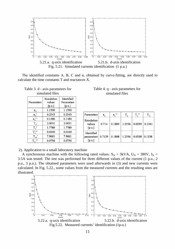
Firstly, the procedure was tested by using known values for simulating a small machine with SIMSEN. The results of the simulation are fed to the identification program, Fig.5.19. The identified parameters were afterward compared to the input values used in SIMSEN. There was a very good accuracy. A difference between known values and identified ones of less then 0.01% was obtained. The identification was made for both axes, Fig.5.21..

11

5.21.a. q-axis identification 5.21.b. d-axis identification

Fig. 5.21. Simulated currents identification (1 p.u.)

The identified constants A, B, C and α, obtained by curve-fitting, are directly used to calculate the time constants T and reactances X.

Table 3. d - axis parameters for

simulated files Table 4. q - axis parameters for

simulated files

2). Application to a small laboratory machine A synchronous machine with the following rated values: SN = 3kVA, UN = 380V, IN =

3.5A was tested. The test was performed for three different values of the current (1 p.u., 2 p.u., 3 p.u.). The obtained parameters were used afterwards in (3) and new currents were calculated. In Fig. 5.22., some values from the measured currents and the resulting ones are illustrated.

5.22.a. q-axis identification 5.22.b. d-axis identification

Fig.5.22. Measured currents’ identification (1p.u.)

12

Table 4. d - axis parameters for 1p.u. Table 5. q - axis parameters for 1 p.u.

B. General case – any rotor position This case is solved starting from three sets of measurements, which will be used to

determine first the rotor position (θ). With three resultant currents and θ, the transversal and longitudinal currents can be separated (id, iq). Now, this case is an application for the first identification procedure. The same program will be used to identify the parameters of the synchronous machine.

1) Determining rotor position Keeping the rotor in the fix, initially unknown position, first phases a and b are supplied

with continuous current, next the other 2 pairs of phases, b and c, c and a, will be supplied with the ‘same’ value of the current. In practice, we can not have exactly the same value for the supplied current. Therefore, we try to have almost the same value and a normalization of the currents is made.

Knowing that the stator flux produced by one of these three resulted currents is:

0 0( ) ( )s s su t dt r i t dtψ

∞ ∞= −∫ ∫

for this short transient period the inductance ls will be: 0

ss

s

liψ

=

Each resulted current (is) is integrated and three inductances are determined. Angle θ’ is

the angle between is and d-axis (fig. 5.10.) and it is: '6

πθ θ= +

The stator inductance of two phases in series is given by the well known relation: ( ') cos 2 'sl l lmθ θ= + ∆

where lm is the median value, ∆ l the half difference of the transversal and longitudinal inductances

2

l lqdlm+

= , 2

l lqdl−

∆ =

13

We have now a system of three equations, from (7), for each pair of phases, with the difference between the three currents of 120° and three unknowns lm, Δl, θ’.

Transversal and longitudinal impedances (ld, lq) can be calculated and for a chosen angle, the impedance l(θ).

Next, the d- and q- inductances are calculated and angle θ’ is found: 1' arccos( )

2

l lmil

θ−

=∆

where li is one of the three inductances and θ’ is the correspondent angle. Next are illustrated the three inductances for the rotor at 20° referred to d-axis. Lt is the theoretical impedance.

Determining the rotor position

Having the rotor position, the three measurements and theirs relations we obtain 3

resultant currents. idmax, iqmax are the currents obtained for the rotor in d-axis, respective q-axis. If we rotate the corresponded vector imax, for the other two positions, equivalent as for AB, BC, CA, we obtain is1, is2, is3.

2 23( ) ( ) co s ( ) sinmaxmax2

i t i t i tqsi i id θ θ′ ′≅ +

Now, from the 3 resulted currents, d- and q- currents can be separated 2 ' 2 '

2 2 112 ' 2 ' 2 ' 2 '

1 2 2 12 ' 2 '

1 2 2 12 ' 2 ' 2 ' 2 '

1 2 2 1

sin sin2max 3 cos sin cos sin

cos cos2max 3 cos sin cos sin

ss

s s

i iid

i iiq

θ θ

θ θ θ θ

θ θ

θ θ θ θ

−≅

−

−≅ −

−

Similar expressions are found for the other pairs of phases. Finally we have idAB, idBC, idCA and iqAB, iqBC, iqCA. When the angle is a multiple of 30°, two of the isi currents are symmetrical referred to d-

and q- axis, the numerator and the denominator are 0. Equations (11) for this situation will not be accepted and the other two will be used. A procedure is written for choosing the appropriate currents used to identify the parameters.

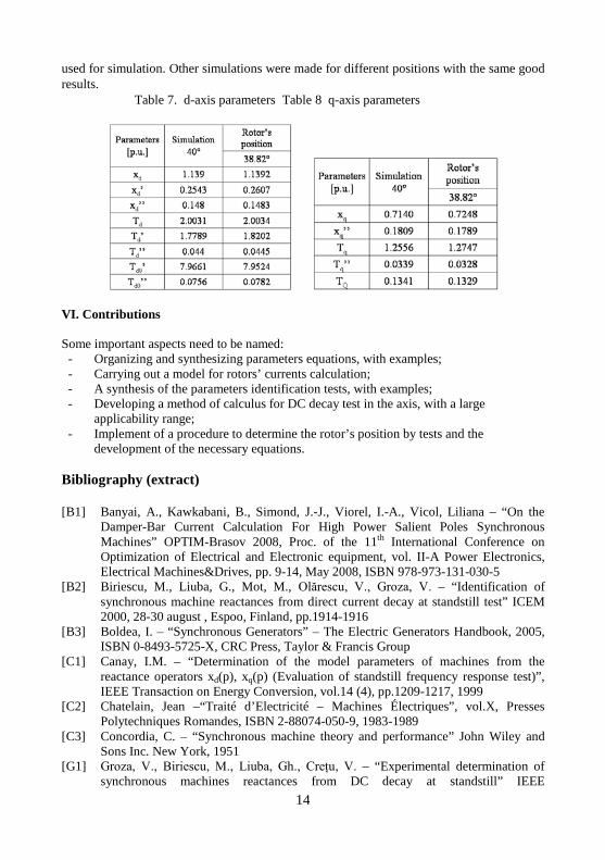
2) Parameters identification for a random position The id and iq currents obtained before are introduced in the same main program. In Table

5 the results for a simulated machine are given. The same parameters as in Table 1 are used, but now, the rotor is positioned at 40°. The obtained parameters are compared with the ones

14

used for simulation. Other simulations were made for different positions with the same good results.

Table 7. d-axis parameters Table 8 q-axis parameters

VI. Contributions Some important aspects need to be named:

- Organizing and synthesizing parameters equations, with examples; - Carrying out a model for rotors’ currents calculation; - A synthesis of the parameters identification tests, with examples; - Developing a method of calculus for DC decay test in the axis, with a large

applicability range; - Implement of a procedure to determine the rotor’s position by tests and the

development of the necessary equations.

Bibliography (extract) [B1] Banyai, A., Kawkabani, B., Simond, J.-J., Viorel, I.-A., Vicol, Liliana – “On the

Damper-Bar Current Calculation For High Power Salient Poles Synchronous Machines” OPTIM-Brasov 2008, Proc. of the 11th International Conference on Optimization of Electrical and Electronic equipment, vol. II-A Power Electronics, Electrical Machines&Drives, pp. 9-14, May 2008, ISBN 978-973-131-030-5

[B2] Biriescu, M., Liuba, G., Mot, M., Olărescu, V., Groza, V. – “Identification of synchronous machine reactances from direct current decay at standstill test” ICEM 2000, 28-30 august , Espoo, Finland, pp.1914-1916

[B3] Boldea, I. – “Synchronous Generators” – The Electric Generators Handbook, 2005, ISBN 0-8493-5725-X, CRC Press, Taylor & Francis Group

[C1] Canay, I.M. – “Determination of the model parameters of machines from the reactance operators xd(p), xq(p) (Evaluation of standstill frequency response test)”, IEEE Transaction on Energy Conversion, vol.14 (4), pp.1209-1217, 1999

[C2] Chatelain, Jean –“Traité d’Electricité – Machines Électriques”, vol.X, Presses Polytechniques Romandes, ISBN 2-88074-050-9, 1983-1989

[C3] Concordia, C. – “Synchronous machine theory and performance” John Wiley and Sons Inc. New York, 1951

[G1] Groza, V., Biriescu, M., Liuba, Gh., Creţu, V. – “Experimental determination of synchronous machines reactances from DC decay at standstill” IEEE

15

Instrumentation and Measurement Technology Conference, Budapest, Hungary, May 21-23, 2001, pp. 1954-1957

[H1] Henneberger, G., Viorel I.-A. – “Variable Reluctance Electrical Machines” Shaker Verlag Aachen, 2001

[K1] Kamwa, I., Viarouge, P. – “On equivalent circuit structures for empirical modeling of turbine-generators” IEEE Trans. on Energy Conv., vol. 9. no. 3, pp. 579-592, 1994

[K2] Keyhani, A., Tsai, H., Pillutla, S. – “Identification of synchronous machine saturated parameters” ELECTROMOTION Journal, vol. 3, nr. 4, oct. - dec. 1996, pp. 155-164

[P1] Park, R.H. – “Two reaction theory of synchronous machines; generalized method of analysis”, AIEE Trans., 1929, 48, (I), pp. 716-728

[S1] Sapin, A., Simond, J.J. – “SIMSEN: A modular software package for the analysis of power networks and electrical machines” Proc. of ICEM 1994, Paris, France

[S2] Simond, J.-J. - “Laminated salient-pole machines: numerical calculation of the rotor impedances, starting characteristics and damper-bar current distribution”, Electric machines and electromechanics, 6:95-108, Hemisphere publishing corporation, 1981

[S3] Soran, I.F., Kisch, D.O., Sârbu, G.M. – “Modelarea sistemelor de conversie a energiei” Ed. ICPE, Bucuresti 1998

[T1] Talaat, M.E. – “A new approach to calculation on synchronous machine reactances” – part. I, AIEE Trans., pt. III, vol. 74, no. 2, pp.176-183, 1955; part. II, AIEE Trans., pt. III, p. 317-327, 1956

[V1] Vicol, Liliana, Banyai, A., Viorel, I.-A., Simond, J.-J. – “On the Damper Cage Bars’ Currents Calculation for Salient Pole Large Synchronous Machines” ADVANCES in Electrical and Electronic Engineering 2008, Zilina, vol.7, no.1-2, pp. 165-170, ISSN – 1336-1376

[V2] Vicol, Liliana, Simond, J.-J., TuXuan, Mai, Viorel, I.-A. – “The Identification of the Synchronous Machine Parameters by Standstill DC Decay Test” Proc. of the XVII International Conference on Electrical Machines, ICEM, Chania, Crete Island, Greece, September 2-5, 2006, CD-ROM

[V3] Vicol, Liliana, Viorel, I.-A. – “Parameters of the Synchronous Generator. Identification Procedures” Proc. of ELS – International Symposium on Electrical Engineering and Energy Converters, 27-28 Sept. 2007, Suceava, p.95, ISBN – 978-973-666-259-1, Ed. Suceava University

[V4] Viorel, I.-A., Vicol, Liliana, Strete, Larisa – “A Comparison between Cage Induction Motor and Variable Reluctance Synchronous Motor with Cageless Segmental Rotor” ICEM 2008, Vilamoura, Portugalia, IEEE Catalog no.: CFP0890B-CDR, ISBN: 978-1-4244-1736-0

[W1] Wiesemen, R.W. – “Graphical determination of magnetic field” AIEE Trans., vol.46, part. 2, 1927, pp.141-154