Testing Multivariate Economic Restrictions Using

Quantiles: The Example of Slutsky Negative

Semide�niteness

Holger Dette�

University of Bochum

Stefan Hoderlein y

Boston College

Natalie Neumeyerz

University of Hamburg

September 27, 2013

Abstract

This paper is concerned with testing rationality restrictions using quantile regression

methods. Speci�cally, we consider negative semide�niteness of the Slutsky matrix, ar-

guably the core restriction implied by utility maximization. We consider a heterogeneous

population characterized by a system of nonseparable structural equations with in�nite

dimensional unobservable. To analyze this economic restriction, we employ quantile re-

gression methods because they allow us to utilize the entire distribution of the data.

Di¢ culties arise because the restriction involves several equations, while the quantile is a

univariate concept. We establish that we may test the economic restriction by considering

quantiles of linear combinations of the dependent variable. For this hypothesis we develop

a new empirical process based test that applies kernel quantile estimators, and derive its

large sample behavior. We investigate the performance of the test in a simulation study.

Finally, we apply all concepts to Canadian microdata, and show that rationality is not

rejected.

Keywords: Nonparametric Testing, Heterogeneity, Integrability, Nonseparable Models, Con-

sumer Demand, Quantile Regression.�Holger Dette, Ruhr-Universität Bochum, Fakultät für Mathematik, 44780 Bochum, Germany, email: hol-

ger.dette@rub.deyStefan Hoderlen, Department of Economics, Boston College, 140 Commonwealth Avenue, Chestnut Hill,

MA 02467, USA, Tel. +1-617-552-6042. email: stefan_hoderlein@yahoo.comzNatalie Neumeyer, University of Hamburg, Department of Mathematics, Bundesstrasse 55, 20146 Hamburg,

Germany, email: neumeyer@math.uni-hamburg.de.

1

1 Introduction

Economic theory yields strong implications for the actual behavior of individuals. In the stan-

dard utility maximization model for instance, economic theory places strong restrictions on

individual responses to changes in prices and wealth, the so-called integrability constraints.

These restrictions are inherently restrictions on individual level: They have to hold for every

preference ordering and every single individual, at any price wealth combination. Other than

obeying these restrictions, the individuals�idiosyncratic preference orderings may exhibit a lot

of di¤erences. Indeed, standard parametric cross section mean regression methods applied to

consumer demand data often exhibit R2 between 0.1 and 0.2. Today, the consensus is that the

majority of the unexplained variation is precisely due to unobserved preference heterogeneity.

For this reason, the literature has become increasingly interested in exploiting all the informa-

tion about unobserved heterogeneity contained in the data, in particular using the quantiles of

the dependent variable.

To lay out our model, let y denote the L � 1 vector of quantities demanded. At this stage,we have already imposed the adding up constraint (i.e., out of L goods we have deleted the

last). Let p denote the L vector of prices, and x denote income (total expenditure)1. For every

individual, de�ne the cost function C(p; u) to give the minimum cost to attain utility level u

facing the L-vector of prices p, and given income (more precisely, total outlay) x: The Slutsky

negative semide�niteness restriction arises from the fact that the cost function is concave, and

hence the matrix of second derivatives is negative semide�nite (nsd, henceforth). For brevity,

we will sometimes equate negative semide�niteness with �rationality", even though it is only

one facet of rationality in this setup with linear budget constraint2.

Obviously, this hypothesis has to hold for any preference ordering u. However we do not observe

the individual�s preference ordering u, and only observe a K dimensional vector of household

covariates (denoted q). Speci�cally, we assume to have n iid observations on individuals from

an underlying heterogeneous population characterized by random variables U; Y;X; P;Q which

have a nondegenerate joint distribution FU;Y;X;P;Q.

The question of interest is now as follows: What can we learn from the observable part of this

distribution, i.e. FY;X;P;Q; about whether the Slutsky matrix is negative semide�nite across a

heterogeneous population, for all values of (p; x; u). In Hoderlein (2011), we consider testing

1This is the income concept commonly used in consumer demand. It is motivated by the assumption of

separability of preferences over time and from other decisions (e.g., the labor supply decision). We use the

phrases �total expenditure", �income" and �wealth�interchangeably throughout this paper.2Since negative semide�niteness is arguably the core rationality restriction, we feel that this shortcut is

justi�ed, but we would like to alert the reader to this.

2

negative semide�niteness in such a setting with mean and second moment regressions only.

However, these lower order moment regressions have the disadvantage that they use only one

feature of FY;X;P;Q, and not the entire distribution. Therefore, in this paper we propose to

exploit the distributional information by using all the �-quantiles of the conditional distribution

of observables, which (with varying �) employ all the information that may be obtained from

the data about the economic hypothesis of interest.

There are two immediate di¢ culties now, and solving them is the major innovation this paper

introduces. The �rst is how to relate a speci�c economic property in the (unobservable) world

of nonseparable functions to observable regression quantiles. The second one is how to use

quantiles in systems of equations. The solution for the second di¢ culty is to consider linear

combinations of the dependent variable, i.e. Y (b) = b0Y for all vectors b of unit length and

consider the respective conditional �-quantiles of this quantity. This can be thought of as an

analogue to the Cramer-Wold device, and is a strategy that is feasible more generally, e.g., when

testing omission of variables. As b and � vary, we exploit the entire distribution of observables.

The solution to the �rst of these two di¢ culties involves obviously identifying assumptions.

To this end, since we are dealing with nonseparable models we require full conditional inde-

pendence, i.e., we require that U? (P;X) jQ, or versions of this assumption that control forendogeneity. These assumptions are versions of the �selection on observables" assumptions in

the treatment e¤ect literature. Essentially they require that, in every subpopulation de�ned

by Q = q, preferences as well as prices and income be independently distributed. Although

endogeneity is not relevant for our application, our treatment covers the control function ap-

proach to handle endogeneity in nonseparable models discussed in Altonji and Matzkin (2005),

Imbens and Newey (2009) or Hoderlein (2011), by simply adding endogeneity controls V to the

set of household control variables Q. From now on, we denote by W the set of all observable

right hand side variables, i.e., (P 0; X;Q0); and potentially in addition V; if we are controlling

for endogeneity3.

Under this assumption and some regularity conditions, our �rst main contribution is as follows:

We establish that the untestable rationality hypothesis in the underlying population has a

testable implication on the distribution of the data, speci�cally, on the conditional quantiles

of linear combinations of the dependent variables. Consequently, we can test a null hypothesis

in the underlying (unobservable) heterogeneous population model in the sense that a rejection

of the testable implication leads also to a rejection of the original null hypothesis. While this

procedure controls size, though likely conservative, it may su¤er from low power: If we do not

3In classical consumer demand, it is typically income that is considered endogenous, see the discussion in

section 2.

3

reject the implication, we cannot conclude that the data could not have been generated by some

other, nonrational mechanism. This is the price we pay for being completely general, as the

only material assumption that we require to relate the observable object and the underlying

heterogeneous population is the conditional independence assumption U ? (P;X) jQ, and noother material assumption on the functional form of demand or their distribution enters the

model. In particular, we have not assumed any monotonicity or triangularity assumption;

there can be in�nitely many unobservables, and they can enter in arbitrarily complicated form;

in a sense, every individual can have its own nonparametric utility function, and hence this

framework is closer to a random functions setup.

Our second main contribution is proposing a quantile regression based nonparametric test

statistic. Speci�cally, we apply the sample counterparts principle to obtain a nonparametric

test statistic of the testable implication, and derive its�large sample properties. We show weak

convergence of a corresponding standardized stochastic process to a Gaussian process and obtain

an asymptotically valid hypothesis test. Moreover, we propose a bootstrap version of our test

statistic which is based on a centered version of the stochastic process to avoid the generation

of bootstrap observations under the null. We adapt the well known idea of residual bootstrap

for our speci�c model and provide arguments for the validity of the bootstrap. Nonparametric

tests involving quantiles are surprisingly scant, and we list the closest references in the following

paragraph. Speci�cally, in a system of equations setup we are the �rst to propose a quantile

based test of an economic hypothesis, and to implement such a test using real world data.

Our test is a pointwise test, meaning that it holds locally forW = w0. The main reason for this

is that we aim at a more detailed picture of possible rejections, provi ding a better description of

the rationality of the population (e.g., one outcome is that negative semide�niteness is rejected

for 20% of the population (= representative positions at which the test is evaluated)). An

alternative is a test that integrates over a certain range of W , a strategy which increases power

at the expense of a less detailed picture of the population. We feel that both strategies are

justi�ed, and leave the latter for future work4.

Literature Testing the key integrability constraints that arise out of utility maximization

dates back at least to the early work of Stone (1954), and has spurned the extensive research

on (parametric) �exible functional form demand systems (e.g., the Translog, cf. Jorgenson, Lau

and Stoker (1982), and the Almost Ideal, cf. Deaton and Muellbauer (1980)). Nonparametric

4At an intermediate stage, we could consider the behavior of the test at a �xed grid of values w1; :::; wB :

Since the pointwise estimators at the di¤erent grid points are asymptotically independent, the present theory

extends straightforwardly, and merely results in a more cumbersome notation. This is why we desist from this

here.

4

analysis of some derivative constraints was performed by Stoker (1989) and Härdle, Hildenbrand

and Jerison (1991), but none of these has its focus on modeling unobserved heterogeneity.

More closely related to our approach is Lewbel (2001) who analyzes integrability constraints

in a purely exogenous setting, but does not use distributional information nor suggests or

implements an actual test. An alternative method for checking some integrability constraints

is revealed preference analysis, see Blundell, Browning and Crawford (2003), and references

therein. An approach that combines revealed preference arguments with a demand function

structure is Blundell, Kristensen and Matzkin (2011). As a side result, this paper develops a

test of the weak axiom of revealed preferences, but in contrast to our paper, this paper assumes

a scalar unobservable that enters monotonically in a single equation setup.

While our approach extends earlier work on demand systems, it is very much a blueprint for

testing all kinds of economic hypothesis in systems of equations. Due to the nonseparable

framework we employ, our approach extends the recent work on nonseparable models - in par-

ticular Hoderlein (2011), Hoderlein and Mammen (2007), Imbens and Newey (2009), Matzkin

(2003). When it comes to dealing with unobserved heterogeneity, there are two strands in

this literature: The �rst assumes triangularity and monotonicity in the unobservables (Chesher

(2003), Matzkin (2003)). The triangularity and monotonicity assumptions are, however, rather

implausible for consumer demand, because in general the multivariate demand function is a

nonmonotonic function of an in�nite dimensional unobservable - the individuals� preference

ordering - and all equations depend on this object.

Hence we follow the second route. Extending earlier work in Hoderlein (2011), Hoderlein and

Mammen (2007) establish interpretation of the derivative of the conditional quantile (a scalar

valued function!) if there is more than one unobservable. The upshot of this work is that in

a world with many di¤erent sources of unobserved heterogeneity, at best conditional average

e¤ects are identi�ed, see also Altonji and Matzkin (2005) and Imbens and Newey (2009).

In the statistics literature, the closest work we are aware of includes the testing procedures

proposed by Zheng (1998), Sun (2006), Escanciano and Velasco (2010), and Dette, Wagener

and Volgushev (2011), which all consider some versions of tests on regression quantiles, but there

is no clear direct relationship. Finally, Wolak (1991) considers testing of inequality constraints

in nonlinear parametric models. These tests are very di¤erent from ours due to the general

di¤erence between testing in parametric and nonparametric environments.

In this paper we work with quantiles of univariate linear combinations of the multivariate

observations. In the literature several di¤erent approaches to de�ne quantiles of multivariate

random variables have been suggested, see Barnett (1976), Ser�ing (2002) and Koenker (2005)

for overviews, and Hallin, Paindaveine and Siman (2010) and Belloni and Winkler (2011) for

5

more recent approaches.

Structure of the Paper: The exposition of this paper is as follows. In the next section,

we introduce our model formally, state some assumptions, and derive and discuss the main

identi�cation result. In the third section, we propose a nonparametric test for the economic

hypothesis of Slutsky nsd based on the principle of sample counterparts, analyze its large sample

behavior and propose a bootstrap procedure to derive the critical values. We investigate the

performance of the bootstrap procedure for moderate sample sizes in a simulation study in

section 4. In the �fth section, we apply these concepts to Canadian expenditure data. The

results are a¢ rmative as far as the validity of the integrability conditions are concerned and

demonstrate the advantages of our framework. A summary and an outlook conclude this paper,

while the appendix contains regularity assumptions, proofs, graphs and summary statistics.

2 Deriving Quantile Restrictions of Economic Behavior

in a Heterogeneous Population

2.1 Building Blocks of the Model and Assumptions

Our model of consumer demand in a heterogeneous population consists of several building

blocks. As is common in consumer demand, we assume that - for a �xed preference ordering

- there is a causal relationship between physical quantities, a real valued random L-vector de-

noted by Y , and regressors of economic importance, namely prices P and total expenditure X,

real valued random vectors of length L and 1; respectively, stemming from utility maximization

subject to a linear budget constraint. More speci�cally, in slight abuse of notation, we de�ne the

Marshallian demand function for an individual with preferences u 2 U , where U is a preferencespace, e.g., the space of r times continuously di¤erentiable utility functions, to be y = (p; x;u).

We consider Slutsky nsd for a (L� 1)�(L� 1) submatrix of the Hessian of the cost function, de-notedDp�L (p; x;u)+rx (p; x;u) (p; x;u)

0 =S(p; x; u) = (sjk(p; x; u))1�j�L�1;1�k�L�1, where

p�L denotes the price vector without the L-th price. If this submatrix of second derivatives is

not nsd, the complete matrix involving all L equations cannot be nsd either. The null hypoth-

esis in the underlying unobservable heterogeneous populations is hence that b0S(p; x; u)b � 0;for all b 2 SL�1 (where here and throughout Sd denotes the d-dimensional unit sphere) andany (u; p; x) 2 U� RL+1: The hypothesis of Slutsky nsd translates therefore to an inequalityrestriction on an L� 1 dimensional system of equations, where each equation is characterized

by a nonseparable model. As already mentioned, we assume a linear budget constraint as well

6

as nonsatiation of preferences, which implies the adding up constraint. To avoid the singularity

associated with this constraint, we impose it from the outset, so that we obtain an L�1 vectorof dependent variables. We also assume homogeneity of degree zero, so that we can omit the

L-th price (that of the residual category, prices have from now on dimension L�1), all prices arerelative to the residual price, and total expenditure is normalized to be real total expenditure.

To capture the notion that preferences vary across the population, we assume that there is

a random variable U 2 U , where U is a Borel space5, which denotes preferences (or more

generally, decision rules). In this setup, all individuals could be of the same type, e.g., Cobb

Douglas, with varying parameters, but they could also have their own type each, which is the

notion that we think is most realistic. We assume that heterogeneity in preferences is partially

explained by observable di¤erences in individuals�attributes (e.g., age), which we denote by

the real valued random K-vector Q. Hence, we let U = #(Q;A); where # is a �xed U-valuedmap de�ned on the sets Q�A of possible values of (Q;A), and where the random variable A

(taking again values in a Borel space A) covers residual unobserved heterogeneity in a generalfashion. To �x ideas, think of A as the genom of an individual.

As already mentioned, we want to allow for in�nitely many individual preference orderings

each of which may be characterized by �nite or in�nite dimensional parameter. Therefore

we formalize the heterogeneous population as Y = (P;X;U) = �(P;X;Q;A); for a general

map � and an in�nite dimensional vector A. Obviously, neither � nor the distribution of A are

nonparametrically identi�ed. Still, for any �xed value of A, say a0, we obtain a demand function

having standard properties. Moreover, to show that our approach can handle endogeneity which

arises because economic decisions are related, we treat the more general case and introduce

additional instruments, denoted S. The prototypical example for endogeneity in a consumer

demand setting is total expenditure X (�income�), in parts because individual expenditures

are often large categories that are mismeasured, and hence the aggregate expenditure measure

is mismeasured, too. The typical instrument S is the wage rate, because it impacts total

expenditure in any given period via a life cycle planning argument, but is determined on the

market largely outside the individual�s in�uence. As the main breadwinner�s labor supply

is often assumed to be inelastic, the argument extends to labor income which is often used

alternatively, see Lewbel (1999). However, the argument could also be extended to some other

source of endogeneity, say, in the own price. To keep the exposition simple, we focus on the

scalar endogenous variable case, i.e. we assume that it is only X that is endogenous, and that

5Technically: U is a set that is homeomorphic to the Borel subset of the unit interval endowed with the Borel�-algebra. This includes the case when U is an element of a polish space, e.g., the space of random piecewise

continuous utility functions.

7

there is exactly one additional instrument S. Note, however, that in our application endogeneity

does not play a major role, and this is done solely for expositional purposes.

The �rst assumption collects all de�nitions and speci�es the DGP formally:

Assumption 1. Let (;F ; P ) be a complete probability space on which are de�ned the randomvectors A : ! A; A � R1; and (Y; P;X;Q; S; V ) : ! Y �P � X �Q� S � V ; Y �RL�1;P � RL�1;X � R;Q � RK ;S � R; V � R, with L and K �nite integers, such that

Y = �(P;X;Q;A);

X = �(P;Q; S; V )

where � : P � X �Q�A ! Y and � : P �Q� S � V ! X are Borel functions, and

realizations of (Y; P;X;Q; S) are observable, whereas those of (A; V ) are not. Moreover, � is

invertible in its last argument, for every (p; q; s):

Assumption A1 de�nes the nonparametric demand system with (potentially) endogenous re-

gressors as a system of nonseparable equations. These models are called nonseparable, because

they do not impose an additive speci�cation for the unobservable random terms (in our case

A ). They have been subject of much interest in the recent econometrics literature (Chesher

(2003), Matzkin (2003), Altonji and Matzkin (2005), Imbens and Newey (2009), Hoderlein

(2011), Hoderlein and Mammen (2007), to mention just a few). Since we do not assume

monotonicity in unobservables and allow the error to be in�nite dimensional, our approach is

more closely related to the latter four approaches. As is demonstrated there, in the absence of

strict monotonicity of � in A, the function � is not identi�ed, however, local average structural

derivatives are. Although it will be demonstrated that identi�cation may proceed on this level

of abstraction, in the case of endogeneity of X this requires, however, that V be solved for

because these residuals have to be employed in a control function fashion. In the application,

we specify � to be the conditional mean function, and consequently V to be the additive mean

regression residuals, but this is only one out of several possibilities. We conjecture that alter-

native approaches are possible where one restricts the dimension of the error in the outcome

equation at the expense of an unrestricted IV equation. Since in our application endogeneity

turns out not to be an issue, we do not want to extend the discussion unnecessary.

Given that we have all major elements of our model de�ned and in place, we specify the

independence conditions required for identi�cation. We introduce the notation Z = (Q0; V )0;

and Z = Q� V.

Assumption 2. The random vectors A and (P;X) are independent conditional on Z.

8

AssumptionA2 is the only material assumption that we require in order to identify the marginal

e¤ect of interest, and thus being able to analyze the economic restriction of interest, in our case

Slutsky negative semide�niteness. Therefore it merits a thorough discussion: Assume for a

moment all regressors were exogenous, i.e. S � X; Z � Q and V � 0. Then this assumptionstates that wealth and prices be independently distributed of unobserved heterogeneity A,

conditional on individual attributes.

To give an example: Suppose that in order to determine the e¤ect of wealth on consumption,

we are given data on the demand of individuals, their wealth and the following attributes:

�education in years� and �gender�. Take now a typical subgroup of the population, e.g.,

females having received 12 years of education. Assume that there be two wealth classes for this

subgroup, rich and poor, and two types of preferences, type 1 and 2. Then, for both rich and

poor women in this subgroup, the proportion of type 1 and 2 preferences has to be identical for

all levels of wealth. This assumption is of course restrictive. Note, however, that preferences

and economically interesting regressors may still be correlated across the population. Moreover,

any of the Z may be correlated with preferences, in particular Q, i.e., household characteristics.

Finally, if it is suspected that regressors and unobservables are not independent, we may still

introduce instruments in a control function fashion.

In the following, to make the exposition less dense we make use of the notationW = (P 0; X;Q0; V 0)0.

Moreover, for a given vector b we introduce the conditional quantile k(�; bjw) of the distrib-ution of Y (b) = b0Y , given W = w, i.e. for 0 < � < 1 the quantity k(�; bjw) is de�ned byP(Y (b) � k(�; bjw) j W = w) = �; or, upon substitution,

P(b0�(p; x; q; A) � k(�; bjw) j W = w) = �;

where w = (p0; x; q0; v0). We will also require a set of regularity assumptions, largely di¤er-

entiability and boundedness conditions, which can be found in the appendix (see assumption

A3). Given these assumptions and notations, we concentrate �rst on the relation of theoretical

quantities and identi�ed (and hence estimable) objects. Speci�cally, we are concerned with the

question of how quantiles allow inference on key elements of economic theory. In particular, we

want to learn about negative semide�niteness of the Slutsky matrix. In the standard consumer

demand setup we consider, the Slutsky matrix in the underlying heterogeneous population

(de�ned by �, x and v), takes the form

S(p; x; u) = Dp (p; x; u) + @x (p; x; u) (p; x; u)0 for all (p; x; u) 2 P � X � U ,

whereD denotes the matrix of second derivatives with respect to price, and @ denotes the vector

of partial derivatives with respect to income. Slutsky negative semide�niteness is an implication

9

of the weak axiom of revealed preferences, and given smooth and di¤erentiable demands, it is

�almost�equivalent in the sense that the usual weak axiom is equivalent to Slutsky negative

de�niteness (i.e., S < 0), and Slutsky negative semide�niteness is equivalent to a weak version

of the weak axiom that allows for weak inequalities in both de�ning equations, see Kihlstrom,

Mas Colell and Sonnenschein (1976). Since we think of our framework as one with continuously

distributed demands and utility functions, the di¤erence is likely a set of measure zero in any

such application. Hence we will loosely refer to both concepts as equivalent, even though

theoretically they are not.

The following theorem provides an answer about what we can learn from regression quantiles.

Theorem 1. Let assumptions A1�A3 hold. Then

S(p; x; u) nsd ) rpk(�; bjw)0b+ @xk(�; bjw)k(�; bjw) � 0

for all (�; b) 2 (0; 1)� SL�1; and all (p; x; u; z) 2 P � X � U � Z. Moreover,

rpk(�; bjw)0b+ @xk(�; bjw)k(�; bjw) = E [b0Sb j W = w; Y (b) = k(�; bjw)] :

Discussion of Theorem 1: This result establishes the link between negative semide�niteness

in a heterogeneous population characterized by complicated and nonmonotonic heterogeneity,

and the joint distribution of the data as characterized by the various regression quantiles of

Y (b) for all b 2 SL�1: As already discussed above, it characterizes all we can learn from data

about the economic hypothesis of interest, and also characterizes the object by which we do, i.e.,

F(�; b; p; x; z) = rpk(�; bjp; x; z)0b+ @xk(�; bjp; x; z)k(�; bjp; x; z): To see the economic contentof F(�; p; x; z), note that the second part of the theorem establishes that this quantity is relatedto the LASD of Hoderlein (2011), and Hoderlein and Mammen (2007). To continue with our

economic example, suppose again we were given data on consumption, wealth, �education in

years�and �gender�as above. Then by considering F(�; b; p; x; z), we may identify, for �xedb, the average over the Slutsky matrix of a subpopulation characterized by a certain level of

prices, wealth and covariates, e.g., all female high school graduates earning 50K, whose value

of a weighted average of their demands has a certain value. However, due to the pervasive and

complex unobserved heterogeneity, we are not able to identify the Slutsky matrix of every single

individual. Thus, since we consider b0Y , our averages use more information than simply the

one embedded in the regressors; by variation of b we consider these averages across the entire

distribution of the data and hence use all information available.

There are limitations to this approach that employs minimal assumptions and these limitations

suggest interesting directions for future research. One particular issue is the following: The

10

equality in theorem 1 provides testable implications for each �xed value (p; x; z), and all quan-

tiles. In this setup, even the entire information contained in the joint distribution of observables

does not su¢ ce to trace out the distribution of unobservables - there is �excess�heterogeneity,

i.e., we cannot invert the distribution of observables for the distribution of unobservables as is

for instance the case in triangular models and linear random coe¢ cient models. Put reversely,

the joint distribution of (W;Y (b)) is still an integral over the underlying complex structural

relationship, where integration is with respect to �many�unobservables that are generally corre-

lated with Q and Y (b). Hence, the integral operation, in fact a conditional averaging operation,

is not invertible. Absent additional functional form or homogeneity assumptions, this average

is the most we can learn from the data, we cannot learn about the individuals�behavior.

One important implication is loss of power. To see this, assume S(P ;X;U) is a.s.-symmetric

to avoid imaginary Eigenvalues. Then, since F(�; bjw) = E [b0S(p;x;U)bjW = w] ; for all

b 2 SL�1, it is impossible for F(�; bjw) to be non-positive for all b 2 SL�1, even if S(P ;X;U)is positive de�nite U jW = w-a.s., i.e., the conditional average cannot be non-positive, if not at

least a small set of positive measureS is negative semide�nite. IfF(�; bjw) is non-positive for allb 2 SL�1, the subpopulation with W = w may either be entirely rational (i.e., H 0

0 : S(P ;X;U)

is negative semide�nite U -a.s. holds), or it may be comprised of two subpopulations, the just

mentioned rational population, and another one that de�es rationality. Whether or not this

second population exists cannot be determined from looking at the aggregate statistic F(�; bjw)alone. Formally, we have, for all b 2 SL�1:

E [b0S(p;x;U)bjW = w] = E [b0S(p;x;U)bjW = w;S not nsd]P [S not nsdjW = w]

+ E [b0S(p;x;U)bjW = w;S nsd]P [S nsdjW = w] ;

and if the left hand side is non-positive, it could arise from P [S not nsdjW = w] or from the

fact that the positive �rst average of the nonrational population is, in our language �overcom-

pensated�by the negative average of the rational part of the subpopulation, weighted with their

respective probabilities. Alternatives that are indistinguishable from H 00 are therefore all nec-

essarily of the type where the second term dominates the �rst, and P [S not nsdjW = w] > 0.

3 From Hypothesis to Test Statistic

In this section we assume we have observed independent data (Yi; Pi; Xi), i = 1; : : : ; n, with the

same distribution as (Y; P;X) 2 RL�1�RL�1�R. We do not treat the additional conditioning onZi as standard nonparametric results extend straightforwardly to this setup by simply adapting

the rates appropriately and - in the case of V - having generated regressors, whose estimation

11

does not a¤ect �rst order asymptotics if we are willing to assume enough smoothness in the

regression of endogenous regressors on instruments, see Sperlich (2009). Since including Z only

makes the notation more cumbersome, all results extend in a straightforward fashion, and we

consider a homogeneous subpopulation in our application, we omit it from now on.

For each �xed w = (p; x) 2 RL�1 �R we want to test negative semi-de�niteness of the Slutskymatrix. To this end we use the notations

kp`(�; b j w) = @p`k(�; b j w)

kx(�; b j w) = @xk(�; b j w);

where k(�; b j w) denotes again the �-quantile of the conditional distribution of Y (b) = b0Y ,

given W = (P;X) = w. As we have seen from the previous subsection, the null hypothesis of

rationality transforms to

H0 :L�1X`=1

b`kp`(�; b j w) + kx(�; b j w)k(�; b j w) � 0 (3.1)

8� 2 (0; 1); b = (b1; : : : ; bL�1)0 2 SL�1:

Now let A be any closed subset of (0; 1). We de�ne the test statistic by

Tn =pnhL+2 sup

�2A;b2SL�1Rn(�; b j w); (3.2)

where

Rn(�; b j w) =L�1X`=1

b`k̂p`(�; b j w) + k̂x(�; b j w)k̂(�; b j w): (3.3)

Here, with notations Wi = (P0i ; Xi)

0 and ��(u) = u(�� Ifu < 0g), the estimators are obtainedfrom the kernel quantile estimation approach

(�̂0; �̂1; �̂2)

= arg min(�0;�1;�2)2R�RL�RL�L

nXi=1

��

�Y 0i b� �0 � �01(Wi � w)� (Wi � w)0�2(Wi � w)

�K�Wi � w

h

�as k̂(�; b j w) = �̂0, k̂p`(�; b j w) = �̂1;`, ` = 1; : : : ; L � 1, and k̂x(�; b j w) = �̂1;L, see Yu and

Jones (1998), Koenker (2005) or Hoderlein and Mammen (2009) among others.

Under the conditions stated in assumption A4 in the appendix, Rn(�; b j w) consistentlyestimates

R(�; b j w) =L�1X`=1

b`kp`(�; b j w) + kx(�; b j w)k(�; b j w)

and we have the following weak convergence result.

12

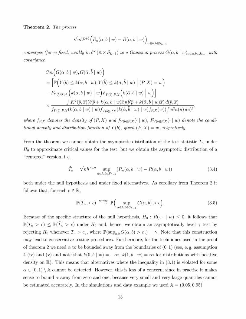
Theorem 2. The process

pnhL+2

�Rn(�; b j w)�R(�; b j w)

��2A;b2SL�1

converges (for w �xed) weakly in `1(A�SL�1) to a Gaussian process G(�; b j w)�2A;b2SL�1 withcovariance

Cov�G(�; b j w); G(~�;~b j w)

�=hP�Y (b) � k(�; b j w); Y (~b) � k(~�;~b j w)

��� (P;X) = w�

� FY (b)jP;X

�k(�; b j w)

��� w�FY (~b)jP;X�k(~�;~b j w) ��� w�i�

RK2(p; x)(b0p+ k(�; b j w)x)(~b0p+ k(~�;~b j w)x) d(p; x)

fY (b)jP;X(k(�; b j w) j w)fY (~b)jP;X(k(~�;~b j w) j w)fP;X(w)(Ru2�(u) du)2

;

where fP;X denotes the density of (P;X) and fY (b)jP;X(� j w), FY (b)jP;X(� j w) denote the condi-tional density and distribution function of Y (b), given (P;X) = w, respectively.

From the theorem we cannot obtain the asymptotic distribution of the test statistic Tn under

H0 to approximate critical values for the test, but we obtain the asymptotic distribution of a

�centered�version, i. e.

~Tn =pnhL+2 sup

�2A;b2SL�1(Rn(�; b j w)�R(�; b j w)) (3.4)

both under the null hypothesis and under �xed alternatives. As corollary from Theorem 2 it

follows that, for each c 2 R,

P( ~Tn > c)n!1�! P

�sup

�2A;b2SL�1G(�; b) > c

�: (3.5)

Because of the speci�c structure of the null hypothesis, H0 : R(�; � j w) � 0, it follows that

P(Tn > c) � P( ~Tn > c) under H0 and, hence, we obtain an asymptotically level test by

rejecting H0 whenever Tn > c , where P(sup�;bG(�; b) > c ) = . Note that this construction

may lead to conservative testing procedures. Furthermore, for the techniques used in the proof

of theorem 2 we need � to be bounded away from the boundaries of (0; 1) (see, e. g. assumption

4 (iv) and (v) and note that k(0; b j w) = �1, k(1; b j w) = 1 for distributions with positive

density on R). This means that alternatives where the inequality in (3.1) is violated for some� 2 (0; 1) n A cannot be detected. However, this is less of a concern, since in practise it makessense to bound � away from zero and one, because very small and very large quantiles cannot

be estimated accurately. In the simulations and data example we used A = (0:05; 0:95).

13

Because of the complicated covariance structure in Theorem 2, in applications we suggest to

approximate the asymptotic quantile c by the following bootstrap procedure.

The idea of any bootstrap procedure for testing hypotheses for independent samples is to gen-

erate new data (Y �k ; P

�k ; X

�k), k = 1; : : : ; n, (independent, given the original sample (Yi; Pi; Xi),

i = 1; : : : ; n) which follow a model as similar as possible to the original data model under the

null hypothesis. However, given the speci�c structure of the null hypothesis it is not clear how to

generate data that ful�ll H0. Instead we use bootstrap versions of the �centered�test statistic~Tn as follows. As is common in regression models, to generate new data we keep the covariates

and de�ne (P �k ; X�k) = (Pk; Xk). For each �xed covariate (Pk; Xk) we then generate Y �

k from a

distribution which approximates the conditional distribution of Y , given (P;X) = (Pk; Xk), i. e.

FY jP;X(� j Pk; Xk). Note that for one-dimensional observations Y this method coincides with

the bootstrap procedure suggested in Hoderlein and Mammen (2009), and consistency may be

established along similar lines. To estimate the conditional distribution FY jP;X(� j Pk; Xk) we

apply the usual kernel approach and de�ne

F̂Y jP;X(y j Pk; Xk) =nXi=1

IfYi;1 � y1; : : : ; Yi;L�1 � yL�1gk�Wi�Wk

g

�Pn

j=1 k�Wj�Wk

g

�for y = (y1; : : : ; yL�1), Yi = (Yi;1; : : : ; Yi;L�1), i = 1; : : : ; n, with kernel function k and bandwidth

g. The bootstrap version of the test statistic Tn de�ned in (3.2) is

T �n =pnhL+2 sup

�2A;b2SL�1

�R�n(�; b j w)�Rn(�; b j w)

�; (3.6)

where Rn is de�ned in (3.3) and R�n is de�ned analogously, but based on the bootstrap sample

(Y �k ; P

�k ; X

�k), k = 1; : : : ; n. Both under the null hypothesis and under alternatives, the condi-

tional distribution of T �n , given the original sample, approximates the distribution of ~Tn de�ned

in (3.4) and (3.5). We approximate the asymptotic quantile c by c�n; , where

P�T �n > c�n;

��� (Yi; Pi; Xi); i = 1; : : : ; n�= :

With the same argument as before (under regularity conditions given in appendix II in A4 and

some assumptions on the kernel k and bandwidth g) we obtain an asymptotically level test

by rejecting H0 whenever Tn > c�n; . Moreover, the test is consistent (against alternatives where

the inequality (3.1) is violated for some � 2 A, b 2 SL�1), because under a �xed alternativesupb;�Rn(b; � j w) converges to supb;�R(b; � j w) > 0 in probability, such that Tn converges toin�nity. On the other hand, c�n; approximates the (1 � )-quantile of ~Tn which converges to

c 2 R by (3.5). Hence, the probability of rejection converges to one.

14

4 Monte Carlo Experiments

To analyze the �nite sample performance of our test statistic and to get a feeling for the

behavior of the test in our application, we simulate data from a joint distribution that has

similar features at least in terms of observables. We specify the DGP to be a linear random

coe¢ cients speci�cation, which is arguably the most straightforward model of a heterogeneous

population, and choose the distributions of coe¢ cients such that under the null the entire

population is rational, while under the alternative there is a fraction that does not have a

negative semide�nite Slutsky matrix. We apply the test developed above to answer the question

whether there is a signi�cant fraction that does not behave rationally.

More speci�cally, to test whether H0 in (3.1) is valid, we �rst estimate Tn as described in

equation (3.2) and the following passage. In particular, in (3.3) we use a local quadratic esti-

mator with a product kernel where the individual kernels are standard univariate Epanechnikov

kernels. The bandwidth is selected by using a slightly larger bandwidth than the bandwidth

that is selected by cross validation of the corresponding nonparametric median regression, to

account for the fact that we largely use derivatives. Since our simulation setup is calibrated to

the application, we use somewhat di¤ering variances for the respective regressors, see below.

To account for this when choosing the bandwidth, we scale the individual bandwidths for every

dimension by multiplying with the standard deviation �Wjof the respective regressor Wj, i.e.,

the bandwidth for dimension j is of the form hj = h�Wj, and h is selected by cross validation

to be approximately 0.25.

To obtain the distribution of T �n from (3.6) we apply the same estimators, but now use 100

bootstrap samples generated as described in section 3. The bandwidth we use is slightly smaller

than the one used in estimation (by a factor of 0.8)6. Since b is supposed to have unit length,

the grid of bs is chosen such that b21+ b22+ b

23 = 1, and b

2j 2 f0; 0:1; ::::; 0:9; 1g ; for all j. We have

evaluated all quantile regressions at a set of 15 equally spaced positions, i.e., A = f0:05; ::::; 0:95gof �-quantiles of Y (b), for every b. We design the test to have nominal level of 0.05, as mentioned

above we will have a slight size distortion by construction. This completes the description of

the econometric tools we apply, and we now turn to the details of the data generating process:

To keep the results simple and transparent, we assume that the data generating process contains

no income e¤ect, and only prices P = (P1; P2; P3; P4)0, P � N (�P ;�P ), where �P = (1; 1; 1; 1)0

and �P = diag(1:6; 1:1; 1:1; 1:6): This is justi�ed as the income e¤ects turn out to be rather

minor in our application, because the individual categories account for moderate sections of

6We have performed some robustness checks by varying the bandwidth, and the results were insensitive to

moderate changes.

15

total expenditures only, and the income elasticities are not very large, see the next section.

In addition to the stochastic regressors, the DGP contains random heterogeneity parameters

A = (A0; A1; A2; A3; A4)0, independent of P; for which we specify that A � N (�A;�A) : We

choose �A = (20; 20; 20; 30; 10)0; the second to fourth reproduce the average absolute values

of the own price e¤ects of prices 1-3 in our application, and �A = diag(5; 5; 5; 5; 2) in the low

variance setup, and �A = diag(5; 10; 5; 5; 2). Those values are chosen, together with the random

coe¢ cients A0 and A4, to roughly reproduce the R2 in the respective regressions. Moreover, we

assume that there is a �xed parameter � 2 R+ which we introduce to model deviations fromthe null of rationality (negative semide�nitness).

The quantities Y = (Y1; Y2; Y3)0 are then generated as2664Y1

Y2

Y3

3775 =26641:5(A0 � 20) + 20

A0

0:8A0

3775+2664�A1 + � 0:4A2 0

0:2A1 �A2 0

0 0 �A3

3775| {z }

Slutsky

2664P1

P2

P3

3775+2664A4

A4

A4

3775P4;

Observe that in this model the Slutsky matrix is given by:

S(A) =

2664�A1 + � 0:4A2 0

0:2A1 �A2 0

0 0 �A3

3775 :For � = 0; the entire population is rational, i.e., its Slutsky matrix is negative semide�nite.

However, as � increases, parts of the population become inde�nite, which in the language of this

paper means that they cease to be rational. The following table illustrates how the proportion

of the population which is not rational increases, as illustrated by the largest (nonnegative)

eigenvalue of the symmetrized version of the Slutsky matrix:

� = 0 10 15 17.5 20 22.5 25 30

% Population not Rational 0.0001 0.041 0.250 0.443 0.647 0.822 0.928 0.996

This exercise corresponds to a mean shift in the distribution of the �rst random coe¢ cient. Al-

ternatively, more nonrational types may also be generated by increasing the variance, however,

for the above reason (proximity to our application), we focus on this speci�cation. From this

model, we draw an iid sample of n = 3000 observations.

The following table shows the result of our procedure as described in the previous paragraphs,

with n = 3000 observations, a bandwidth of 0:25, and at mean values of the regressors, � =

16

(1; 1; 1; 1). The size of the test is 0.03, and the power is displayed at the following alternatives:

� = 10 15 17:5 20 22:5 25 30

% Population not Rational 0:041 0:250 0:443 0:647 0:822 0:928 0:996

Power 0:170 0:310 0:420 0:590 0:770 0:900 0:970

Figure 1 in the appendix gives a graphical representation of these results, as function of �;

while �g.2 displays the power as a function of the proportion of the population that violates

rationality. If we increase the bandwidth somewhat, the results do not change signi�cantly,

however, eventually the power decreases. In contrast, the results are sensitive to the choice of

bandwidth in the sense that we get size distortions if we choose too small a bandwidth, more

precisely, the size becomes 0:110. The following table shows the result of decreasing h from

0:25 to 0.2.

� = 10 15 17:5 20 22:5 25 30

% Population not Rational 0:041 0:250 0:443 0:647 0:822 0:928 0:996

Power 0:190 0:310 0:390 0:580 0:770 0:880 0:940

The results are graphically compared in �g. 3 in the appendix. Finally, to show the consistency

of the test, we display the result with n = 6000. At the now somewhat smaller bandwidth of

h = 0:2, we obtain a size of 0:04 and the following results on power:

� = 10 15 17:5 20 22:5 25 30

% Population not Rational 0:041 0:250 0:443 0:647 0:822 0:928 0:996

Power 0:240 0:380 0.530 0:640 0:800 0:910 0:980

We also perform the result for n = 1500; and they show a comparable decrease in power. A

graph summarizing power as a function of n is displayed in �g. 4 in the appendix. Obviously

the test exhibits power and is consistent for � bounded away from zero and one7. Moreover,

the power should also be seen in the context that the true model is a linear random coe¢ cient

model. It is well known from the nonseparable models literature that there is a tight connection

between quantiles and nonlinear models with one monotonic heterogeneity factor, a class of

models that is very di¤erent from our DGP. Finally, note that these deviations from rationality

are rather mild; even amongst the non rational people most of the individuals exhibit small

7As already mentioned, this means that the test is not consistent against alternatives where the inequality

in (3.1) is violated for some � 2 (0; 1) n A. However, this is less of a concern, since in our application it makessense to bound � away from zero and one, because very small and very large quantiles cannot be estimated

accurately

17

positive values of the Slutsky matrix. It is easy to design Monte Carlo experiments in which a

larger positive eigenvalue of a small fraction of the population would generate even more power

for our test, however, we do not believe that this represents a feature of our application, and

hence desist from doing so here. In summary, we would also not expect that our test exhibits

too much power against this speci�cation, and the results appear reasonable.

However, this speci�cation of the DGP allows easier comparison with standard practise, without

which our results are hard to interpret. Since, to the best of our knowledge, there is no work

which even mildly resembles what we propose, we compare our approach with a stylized version

of standard parametric methods in this setup. Speci�cally, we run a parametric regression using

a FGLS approach. Given our setup, the FGLS estimator incorporates the entire information

about the model, as it is the ML estimator8. We then compute the largest eigenvalue of the

Slutsky matrix, say, �̂. Finally, we implement a bootstrap procedure to obtain standard errors,

which is appropriate if there is no multiplicity of eigenvalues. The point estimate of the largest

eigenvalue for � = 17:5 is �0:871, with 95% con�dence interval [�1:189;�0:549]. For � = 22:5,the point estimate is 3.809, with 95% con�dence interval [3:480; 4:129]. To perform a one

sides test, we moreover construct critical values CV = 2�̂�Q(:95; F�̂���̂); where Q(:95; F�̂���̂)denotes the 95% quantile of F�̂���̂. For � = 17:5; we obtain an average CV = �1:193, and zerorejections, whereas for � = 22:5; we obtain an average CV = 3:488 with universal rejections.

Standard practise would hence not reject, if 45% of the population is not rational and always

reject with 80% nonrational individuals. The reason for this di¤erence is that the parametric

approach implicitly aggregates, and rejects only if the aggregate is su¢ ciently non rational after

which it always rejects due to its small standard errors. This is di¤erent from our approach,

which at least conditions on all observable information, and hence provides a smoother function

in the fraction of nonrational people.

An interesting conclusion out of this comparison is that standard practise in parametric models

picks up deviations from rationality only if it has �nally an impact on the mean. In contrast, our

test exhibits power already if the fraction of the population being not rational is rather small

(e.g., with 4% non rational individuals and n = 6000, a typical size in a cross section application,

we reject one quarter of times). Rather than signi�cant parts of the population being wildly

non rational, we believe that at best parts of the population deviate from rationality in a rather

mild fashion, and given the simulation results we feel comfortable that our test will be able to

detect these deviations in an application, at least if we perform it at a large set of independent

positions. Let us therefore now turn to such an application.

8We are indebted to Dennis Kristensen for this suggestion

18

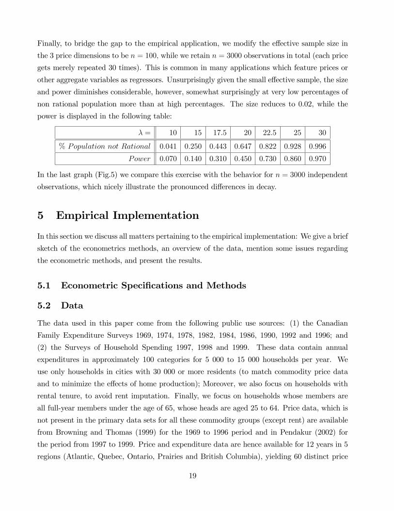
Finally, to bridge the gap to the empirical application, we modify the e¤ective sample size in

the 3 price dimensions to be n = 100; while we retain n = 3000 observations in total (each price

gets merely repeated 30 times). This is common in many applications which feature prices or

other aggregate variables as regressors. Unsurprisingly given the small e¤ective sample, the size

and power diminishes considerable, however, somewhat surprisingly at very low percentages of

non rational population more than at high percentages. The size reduces to 0.02, while the

power is displayed in the following table:

� = 10 15 17:5 20 22:5 25 30

% Population not Rational 0:041 0:250 0:443 0:647 0:822 0:928 0:996

Power 0:070 0:140 0.310 0:450 0:730 0:860 0:970

In the last graph (Fig.5) we compare this exercise with the behavior for n = 3000 independent

observations, which nicely illustrate the pronounced di¤erences in decay.

5 Empirical Implementation

In this section we discuss all matters pertaining to the empirical implementation: We give a brief

sketch of the econometrics methods, an overview of the data, mention some issues regarding

the econometric methods, and present the results.

5.1 Econometric Speci�cations and Methods

5.2 Data

The data used in this paper come from the following public use sources: (1) the Canadian

Family Expenditure Surveys 1969, 1974, 1978, 1982, 1984, 1986, 1990, 1992 and 1996; and

(2) the Surveys of Household Spending 1997, 1998 and 1999. These data contain annual

expenditures in approximately 100 categories for 5 000 to 15 000 households per year. We

use only households in cities with 30 000 or more residents (to match commodity price data

and to minimize the e¤ects of home production); Moreover, we also focus on households with

rental tenure, to avoid rent imputation. Finally, we focus on households whose members are

all full-year members under the age of 65, whose heads are aged 25 to 64. Price data, which is

not present in the primary data sets for all these commodity groups (except rent) are available

from Browning and Thomas (1999) for the 1969 to 1996 period and in Pendakur (2002) for

the period from 1997 to 1999. Price and expenditure data are hence available for 12 years in 5

regions (Atlantic, Quebec, Ontario, Prairies and British Columbia), yielding 60 distinct price

19

vectors. Rent prices for the corresponding periods are from CANSIM (see Pendakur (2002) for

details). Prices are normalized so that the price vector facing residents of Ontario in 1986 is

(1; :::; 1). The data is hence a repeated cross section; every individual is only sampled once.

Table 1 gives (unweighted) summary statistics for 6952 observations of rental-tenure unattached

individuals aged 25-64 with no dependents. Estimated nonparametric densities (not reported,

but available from the authors) for log-prices and log-expenditures are approximately normal,

as is typically found in the demand literature. Analysis is restricted to these households to

minimize demographic variation in preferences. Demographic variation could be added to

the model by conditioning all levels, log-price derivatives and log-expenditure derivatives on

demographic covariates. Rather than pursue this strategy, we use a sample with very limited

demographic variation.

The empirical analysis uses annual expenditure in four expenditure categories: Food at home,

Food Out, Rent and Clothing. This yields three independent expenditure share equations which

depend on 4 prices and expenditure. These four expenditure categories account for about half

the current consumption of the households in the sample in total, and are henceforth called

�Total Expenditure�. Estimation of this sub-demand system is only valid under the assumption

of weak separability of the included four goods from all the excluded goods. As is common

in the estimation of consumer demand, we invoke weak separability for the estimation that

follows, but do not test it.

Table 1: The Data Min Max Mean Std Dev

Expenditure Shares Food at Home 0.02 0.84 0.23 0.11

Food Out 0.00 0.75 0.11 0.10

Rent 0.01 0.97 0.54 0.14

Clothing 0.00 0.61 0.12 0.09

Total Expenditure 640 40270 8596 4427

Prices Food at Home 0.2436 1.4000 1.0095 0.315

Food Out 0.2328 1.7050 1.1260 0.412

Rent 0.2682 1.4423 0.9312 0.321

TotExp in 10K$ 0.0640 4.0270 0.8600 0.428

As another descriptive means to characterize the data, we report the results of three log-log

mean regressions. In our framework, the coe¢ cients do at best re�ect some averages of e¤ects

20

(in the case of endogeneity, not even this is warranted), and are only meant to be informative,

as well as provide consistency checks for the data.

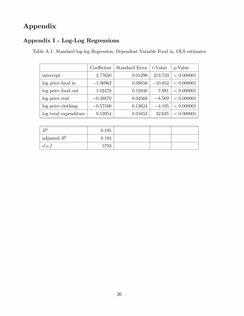
Table A.1 reports the result of the regression of log food in on the four log prices and log total

expenditure. The own price elasticity is around -1, which is in line with reported results for

other good (e.g., gasoline, see Hausman and Newey (1995)). Food in and food out are strong

gross substitutes, as is to be expected, while the substitution patterns with the other goods are

much less pronounced. In fact, if anything, rent and food in seem to be complements; a fact

that may be related to a common lifestyle. Finally, the rather low total expenditure elasticity

is also well documented in other studies, see Lewbel (1999) for an overview. It is shared

by other necessities, e.g., gasoline (Hausman and Newey (1995)). Given the large number of

observations, the estimates are fairly precise.

The other two regressions mirror these �ndings. Food out is less of a necessity than food in,

consequently, its own price elasticity is larger in absolute values, see table A.2. Moreover,

there is only a very weak relationship between food out and rent, which is con�rmed by both

regressions in tables A.2 and A.3. In both instances, the total expenditure elasticities are larger

in absolute value, which is not surprising given that satiation is less of an issue with food out

and rent, which consequently have more of a luxury character. The own price elasticities are

both solidly negative and dominate in absolute value.

Linear quantile regressions essentially reproduce these results. As an example, we have included

the median regression of food out on the same variable in table A.4. Obviously, the results

are very comparable. The variations across quantiles are also surprisingly low. In particular,

the dominant negative diagonal in the Slutsky matrix is well preserved throughout the range

of quantiles. Though our analysis is nonparametric, uses levels as opposed to logarithms, and

considers the compensated as opposed to the uncompensated price e¤ect matrix, the descriptive

results foreshadow our main �nding: the data are largely consistent with the Slutsky matrix

being negative semide�nite across the population.

Finally, as regards endogeneity of total expenditure: Haag, Hoderlein and Pendakur (2009) do

not �nd evidence of endogeneity of total expenditure, the relevant income de�nition in this

setup (see Lewbel (1999)), in this data set. Speci�cally, Haag, Hoderlein and Pendakur (2009)

estimate the residuals in the IV equation nonparametrically, and then use these residuals in a

nonparametric regression of the various demands on total expenditure as additional regressors.

Using a standard nonparametric omission of variables test, they do not �nd the residuals to be

signi�cant. We hence do not pursue any control function strategy in this paper (even though

it would be straightforward given the theoretical results).

21

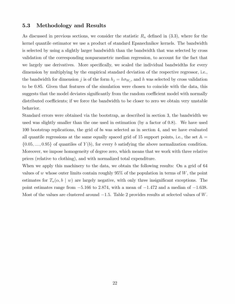
5.3 Methodology and Results

As discussed in previous sections, we consider the statistic Rn de�ned in (3.3), where for the

kernel quantile estimator we use a product of standard Epanechnikov kernels. The bandwidth

is selected by using a slightly larger bandwidth than the bandwidth that was selected by cross

validation of the corresponding nonparametric median regression, to account for the fact that

we largely use derivatives. More speci�cally, we scaled the individual bandwidths for every

dimension by multiplying by the empirical standard deviation of the respective regressor, i.e.,

the bandwidth for dimension j is of the form hj = h�Wj, and h was selected by cross validation

to be 0.85. Given that features of the simulation were chosen to coincide with the data, this

suggests that the model deviates signi�cantly from the random coe¢ cient model with normally

distributed coe¢ cients; if we force the bandwidth to be closer to zero we obtain very unstable

behavior.

Standard errors were obtained via the bootstrap, as described in section 3, the bandwidth we

used was slightly smaller than the one used in estimation (by a factor of 0.8). We have used

100 bootstrap replications, the grid of bs was selected as in section 4, and we have evaluated

all quantile regressions at the same equally spaced grid of 15 support points, i.e., the set A =f0:05; ::::; 0:95g of quantiles of Y (b), for every b satisfying the above normalization condition.Moreover, we impose homogeneity of degree zero, which means that we work with three relative

prices (relative to clothing), and with normalized total expenditure.

When we apply this machinery to the data, we obtain the following results: On a grid of 64

values of w whose outer limits contain roughly 95% of the population in terms of W , the point

estimates for Tn(�; b j w) are largely negative, with only three insigni�cant exceptions. Thepoint estimates range from �5:166 to 2:874, with a mean of �1:472 and a median of �1:638.Most of the values are clustered around �1:5. Table 2 provides results at selected values of W .

22

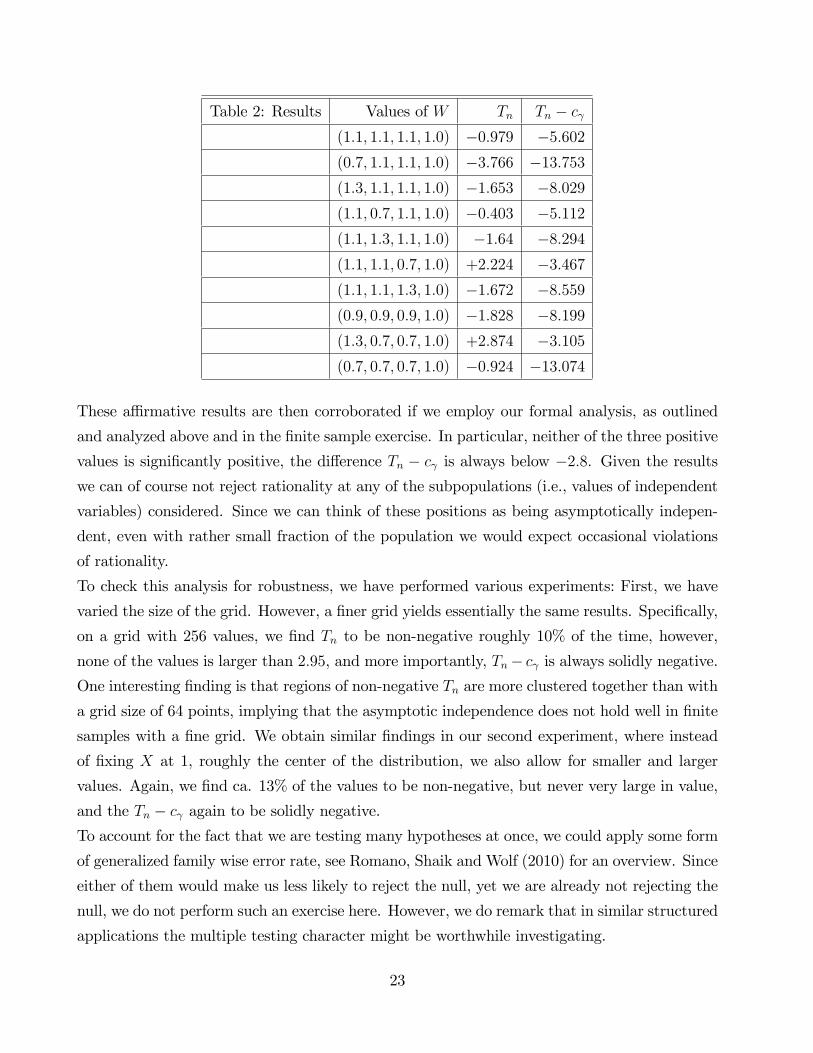
Table 2: Results Values of W Tn Tn � c

(1:1; 1:1; 1:1; 1:0) �0:979 �5:602(0:7; 1:1; 1:1; 1:0) �3:766 �13:753(1:3; 1:1; 1:1; 1:0) �1:653 �8:029(1:1; 0:7; 1:1; 1:0) �0:403 �5:112(1:1; 1:3; 1:1; 1:0) �1:64 �8:294(1:1; 1:1; 0:7; 1:0) +2:224 �3:467(1:1; 1:1; 1:3; 1:0) �1:672 �8:559(0:9; 0:9; 0:9; 1:0) �1:828 �8:199(1:3; 0:7; 0:7; 1:0) +2:874 �3:105(0:7; 0:7; 0:7; 1:0) �0:924 �13:074

These a¢ rmative results are then corroborated if we employ our formal analysis, as outlined

and analyzed above and in the �nite sample exercise. In particular, neither of the three positive

values is signi�cantly positive, the di¤erence Tn � c is always below �2:8. Given the resultswe can of course not reject rationality at any of the subpopulations (i.e., values of independent

variables) considered. Since we can think of these positions as being asymptotically indepen-

dent, even with rather small fraction of the population we would expect occasional violations

of rationality.

To check this analysis for robustness, we have performed various experiments: First, we have

varied the size of the grid. However, a �ner grid yields essentially the same results. Speci�cally,

on a grid with 256 values, we �nd Tn to be non-negative roughly 10% of the time, however,

none of the values is larger than 2:95, and more importantly, Tn� c is always solidly negative.One interesting �nding is that regions of non-negative Tn are more clustered together than with

a grid size of 64 points, implying that the asymptotic independence does not hold well in �nite

samples with a �ne grid. We obtain similar �ndings in our second experiment, where instead

of �xing X at 1, roughly the center of the distribution, we also allow for smaller and larger

values. Again, we �nd ca. 13% of the values to be non-negative, but never very large in value,

and the Tn � c again to be solidly negative.

To account for the fact that we are testing many hypotheses at once, we could apply some form

of generalized family wise error rate, see Romano, Shaik and Wolf (2010) for an overview. Since

either of them would make us less likely to reject the null, yet we are already not rejecting the

null, we do not perform such an exercise here. However, we do remark that in similar structured

applications the multiple testing character might be worthwhile investigating.

23

Of course, our �ndings could merely be an issue of low power. In particular, some of the more

positive values could be in fact signi�cantly positive. However, as already discussed above,

under the minimal assumptions this power issue is unavoidable. What could be done is to

integrate/average over at least parts of the set of conditioning variables. Since the negative

values vastly outweigh the positive, we would expect such an averaging would result in negative

estimates, but we leave such an approach that would extend the work of Haag, Hoderlein and

Pendakur (2009) to quantiles for future research.

6 Summary and Outlook

Rationality of economic agents is the central paradigm of economics. Yet, within this paradigm

individuals can vary widely in their actual behavior; only the qualitative properties of individual

behavior are constrained, but not the heterogeneity across individuals. Indeed, in many data

sets there are large di¤erences in observed consumer choices even for individuals which are

equal in terms of their observed household covariates, like age, gender, educational background

etc.

One of the core qualitative restrictions of Economics is the negative semide�niteness of the

Slutsky matrix. It is the core restriction arising out of (static) utility maximization subject

to a linear budget constraint. This paper discusses how to test this property using the entire

conditional distribution of the data when individuals are assumed to be rational, but other-

wise are allowed to be completely di¤erent from each other. The key insight is that quantile

regressions based on linear combinations of the original dependent variables may be used to

test the property of interest. While some of the insights of this paper may be generalized to

related questions like omission of variables in system of equations (e.g., supply and demand

systems), our focus in this paper remains on negative semide�niteness. We derive the large

sample behavior of the speci�c test statistic we consider, and analyze its small sample behavior

in a simulation study.

Our empirical �ndings emphasize the a¢ rmative tendency in the studies of rationality in Blun-

dell, Pashardes andWeber (1993), Hoderlein (2011), and Haag, Hoderlein and Pendakur (2009).

Using Canadian data, we cannot reject negative semide�niteness. As a caveat, we have seen

from the simulation study that the test may not detect very small fractions of irrational indi-

viduals in the population. While this may be a minor issue given the large set of independent

conditions we are considering, it should nevertheless be seen as encouragement to perform a

similar analysis with other data sets. Also, it may be interesting to search for semiparamet-

ric structures, e.g., random coe¢ cient models that allow to test negative semide�niteness in

24

a heterogeneous population with tests of higher power. Similarly, the structure of panel data

may be exploited with new models that are either more e¢ cient due to a repeated observations

structure, or less prone to model misspeci�cation as they allow for correlated time invariant

factors. We hope that this research will encourage future work in this direction.

Acknowledgements The authors have received helpful comments from the co-editor Han

Hong, an anonymous associate editor and two anonymous referees, Andrew Chesher, Roger

Koenker, Dennis Kristensen, Arthur Lewbel, Rosa Matzkin, Ulrich Mueller, Whitney Newey

and Azeem Shaik, as well as seminar participants at Boston College, Princeton and the Confer-

ence on Nonparametrics and Shape Constraints at Northwestern University. We are particularly

indebted to Krishna Pendakur to provide us with the data. We would also like to thank Martina

Stein, who typed parts of this manuscript with considerable technical expertise. This work has

been supported in part by the Collaborative Research Center �Statistical modeling of nonlinear

dynamic processes�(SFB 823) of the German Research Foundation (DFG).

25

Appendix

Appendix I - Log-Log Regressions

Table A.1: Standard log-log Regression, Dependent Variable Food in, OLS estimates

Coe¢ cient Standard Error t-Value p-Value

intercept 2:77650 0:01299 213:733 < 0:000001

log price food in �1:06962 0:09856 �10:852 < 0:000001

log price food out 1:02478 0:12840 7:981 < 0:000001

log price rent �0:38870 0:04568 �8:509 < 0:000001

log price clothing �0:57160 0:13624 �4:195 < 0:000001

log total expenditure 0:53954 0:01653 32:635 < 0:000001

R2 0:195

adjusted R2 0:194

d:o:f: 5793

26

Table A.2: Standard log-log Regression, Dependent Variable Food Out, OLS estimates

Coe¢ cient Standard Error t-Value p-Value

intercept 2:49445 0:02295 108:673 < 0:000001

log price food in 1:01379 0:17415 5:821 < 0:000001

log price food out �1:64400 1� 0:22688 �7:246 < 0:000001

log price rent �0:05472 0:0807 �0:678 0:4980145

log price clothing �1:37527 0:24074 �5:713 < 0:000001

log total expenditure 1:73781 0:02921 59:490 < 0:000001

R2 0.4176

adjusted R2 0.4171

d:o:f: 5793

27

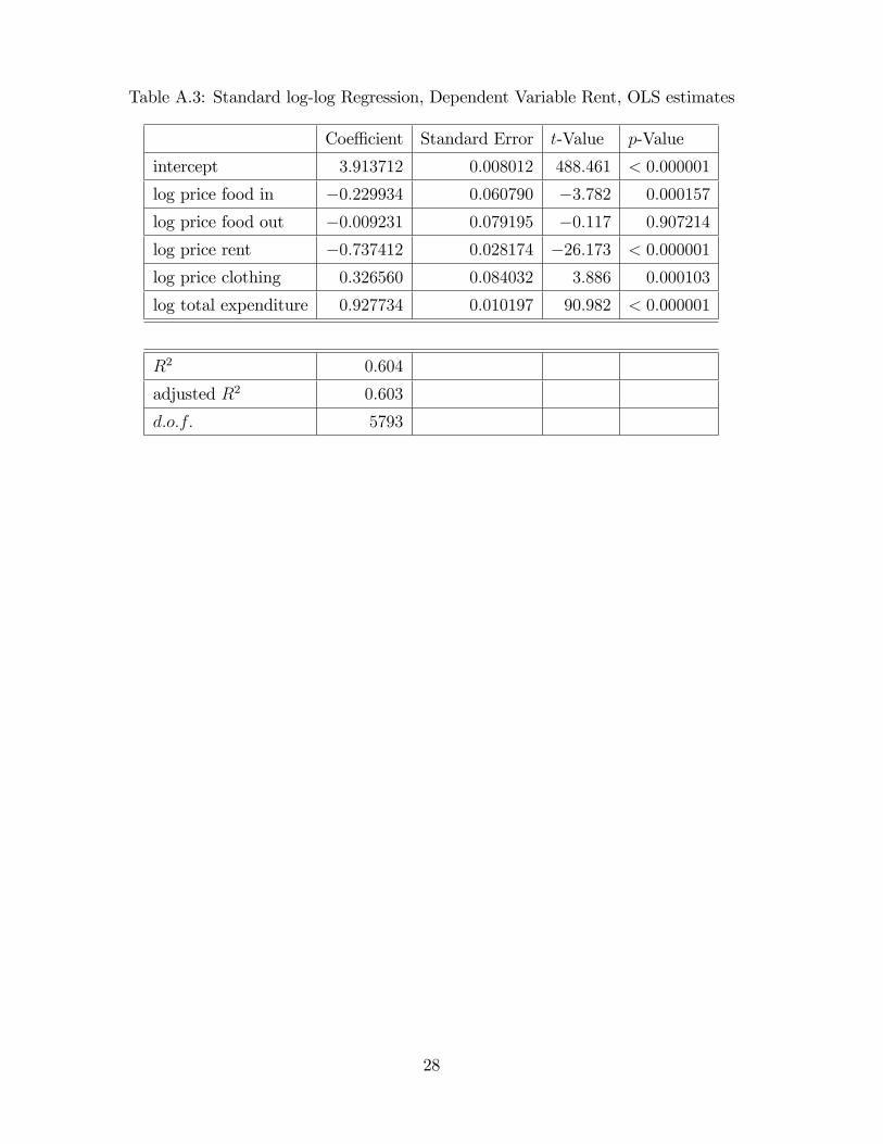
Table A.3: Standard log-log Regression, Dependent Variable Rent, OLS estimates

Coe¢ cient Standard Error t-Value p-Value

intercept 3:913712 0:008012 488:461 < 0:000001

log price food in �0:229934 0:060790 �3:782 0:000157

log price food out �0:009231 0:079195 �0:117 0:907214

log price rent �0:737412 0:028174 �26:173 < 0:000001

log price clothing 0:326560 0:084032 3:886 0:000103

log total expenditure 0:927734 0:010197 90:982 < 0:000001

R2 0:604

adjusted R2 0:603

d:o:f: 5793

28

Table A.4: Linear Quantile log-log Regression, Dependent Variable Food Out, Median

Coe¢ cient Standard Error t-Value p-Value

intercept 2:61447 0:02739 95:46997 < 0:000001

log price food in 1:03697 0:21259 4:87776 < 0:000001

log price food out �1:65577 0:28291 �5:85254 < 0:000001

log price rent �0:04897 0:09972 �0:49107 0:62340

log price clothing �1:48867 0:29715 �5:00975 < 0:000001

log total expenditure 1:84493 0:03762 49:03717 < 0:000001

29

Appendix II - Assumptions

Regularity Conditions for Theorem 1

Assumption 3. For �xed values (p�; x�; z�) 2 P � X � Z and 0 < � < 1 we will make use of

the following assumptions:

(i) The conditional distribution of Y (b) given (P;X;Z) is absolutely continuous w.r.t. the

Lebesgue measure for (p; x) in a neighborhood of (p�; x�) and for z = z�.

(ii) The conditional density fY (b)jPXZ(yjp; x; z�) of Y (b) given (P;X;Z) is continuous in (y; p; x)at the point (k�(w�; b); w�).

(iii) The conditional density fY (b)jPXZ(yjw�; z�) of Y (b) given W = w� is bounded in y 2 R.(iv) Let w1 = (p0; x)

0. k�(w1; z; b) is partially di¤erentiable with respect to any component of

w1 at (w1; z) = (w�1; z�). Moreover, there exist measurable functions �k; k = 1; ::; L, satisfying

P[j�(w�1k + �; w��1k; z�; A)� �(w�1; z

�; A)� ��k(A)j � "�k j X = x�] = o(�k)

for �k ! 0 and �xed " > 0. We write @w1k�(w�1; z

�; a) for �k(a) and @wk� for �k(A), for all

k = 1; ::; L:

(v) The conditional distribution of (Y (b); @w1k�), given (P;X;Z), is absolutely continuous w.r.t.

the Lebesgue measure for (p; x; z) = (p�; x�; z�) and all (b; k). For the conditional density

fY (b);@w1k�jPXZ of (Y (b); @w1k�) given (P;X;Z); we require that fY (b);@w1k�jPXZ(y; y0jp�; x�; z�) �

Cg(y0), where C is a constant and g a positive density on R with �nite mean (i.e.Rjy0jg(y0) dy0 <

1).

Assumptions for Theorem 2

Assumption 4. In the following let A denote a closed subset of (0; 1) and SL�1 = fb 2 RL�1 jjjbjj = 1g. Let W � RL denote the support of W = (P;X) and let w 2 W be �xed. Let

FY (b)jW (� j ~w) and fY (b)jW (� j ~w) denote the conditional distribution and density functions ofY (b) = b0Y , given W = ~w, respectively. For � > 0, M > 0, let C�M(W) denote the class ofsmooth functions with partial derivatives up to order � (the greatest integer smaller than �)

uniformly bounded by M , whose highest partial derivatives are Lipschitz continuous of order

� � � [see van der Vaart and Wellner (1996), p. 154/155]. We will make use of the following

assumptions:

(i) Let K be an L-variate product kernel of the univariate bounded symmetric density � with

bounded support such thatRR �(u)u

2 du <1.(ii) Let h = hn denote a sequence of positive bandwidths such that nh

L(1+ 1L+5

) �! 1,nhL+6 �! 0 for n!1.

30

(iii) Let W be compact and convex and let the density fW of W be bounded away from zero

in a neighborhood N of w and be bounded and continuous. Let the second moments of W exist.

(iv) Assume that the function A� SL�1 ! R, (�; b) 7! k(�; b j w) is bounded by a constant Cand uniformly continuous.

(v) For each �xed ~w 2 W let the function A � SL�1 ! R, (�; b) 7! FY (b)jW (k(�; b j w) j ~w) becontinuous. Assume that there exist M > 0 and � > L

2such that for all c 2 R, jcj � C the

function W ! R, ~w 7! FY (b)jW (c j ~w) belongs to C�M(W). Let the function (y; ~w) 7! fY (b)jW (y j~w) be uniformly continuous in y and ~w and be bounded and bounded away from zero. Further

assume that inf(�;b; ~w)2A�SL�1�N fY (b)jW (k(�; b j ~w) j ~w) > 0 .

Appendix III - Proof of Theorem 1

Let A(!); ! 2 ; denote any random matrix. If b0A(!)b � 0 for all ! 2 and all b 2 RL; then,upon taking expectations w.r.t. an arbitrary probability measure F; it follows thatZ

b0A(!)bF (d!) � 0, b0ZA(!)F (d!)b � 0; for all b 2 SL�1:

From this, S(p; x; u) nsd ) E [SjP = p;X = x; Z = z; Y (b) = k(�; bjw)] nsd for all (p; x; z) 2P � X � Z is immediate. Let E [SjP;X;Z; Y (b)] = B; and note that since the de�nition of

negative semide�niteness of a square matrix B of dimension L� 1 involves the quadratic form,b0Bb � 0. Next, observe that

B = E [SjP = p;X = x; Z = z; Y (b) = k(�; bjw)]

= E [Dp�jP = p;X = x; Z = z; Y (b) = k(�; bjw)]

+ E [@x��0jP = p;X = x; Z = z; Y (b) = k(�; bjw)]

= B1 +B2;

as well as

b0B1b = b0E [Dp�jP = p;X = x; Z = z; Y (b) = k(�; bjw)] b

= E [rp�jP = p;X = x; Z = z; Y (b) = k(�; bjw)] b

= rpk(�; bjw)0b;

31

where � = �0b and the last equality follows from the theorem in Hoderlein and Mammen (2007).

Moreover, by arguments as above

b0B2b = E [b0@x��0bjP = p;X = x; Z = z; Y (b) = k(�; bjw)]

= E [@x��jP = p;X = x; Z = z; Y (b) = k(�; bjw)]

= E [@x�jP = p;X = x; Z = z; Y (b) = k(�; bjw)] k(�; bjw)

= @xk(�; bjw)k(�; bjw);

where the second to last equality follows from Y (b) = � and the last equality again from

Hoderlein and Mammen (2007). Using the de�nition of negative semide�niteness,

b0 (B1 +B2) b � 0;

we obtain,

rpk(�; bjw)0b+ @xk(�; bjw)k(�; bjw) � 0

and the result follows. �

Appendix IV - Proof of Theorem 2

Auxiliary results

Lemma 6.1. Uniformly with respect to � 2 A; b 2 SL�1 we havepnhL+2

�Rn(�; � j w)�R(�; � j w)

�= ~Rn + op(1);

where

~Rn(�; b) =pnhL+2

� L�1X`=1

b`(k̂p`(�; b j w)�kp`(�; b j w))+(k̂x(�; b j w)�kx(�; b j w))k(�; b j w)�:

Proof of Lemma 6.1. The assertion follows from uniform consistency of the estimator k̂x(�; b jw) and

sup�;bjk̂(�; b j w)� k(�; b j w)j = op(

1pnhL+2

):

�

Lemma 6.2. (Bahadur expansion) Uniformly with respect to � 2 A; b 2 SL�1 we have

~Rn(�; b) = � 1pnhL+2

1

fY (b)jP;X(k(�; b j w) j w)fW (w)Ru2�(u) du

nXi=1

K�Wi � w

h

��IfYi(b) � k(�; b j w)g � FY (b)jW (k(�; b j w) j Wi)

��hb0(Pi � p) + k(�; b j w)(Xi � x)

i+ op(1):

32

Proof of Lemma 6.2. Obviously it is su¢ cient to prove the representation for k̂p`(�; b j w)�kp`(�; b j w), ` = 1; : : : ; L� 1, and k̂x(�; b j w)� kx(�; b j w))k(�; b j w) in the representation of~Rn(�; b) in Lemma 6.1, and the assertion of the Lemma follows by building linear combinations.

For the sake of brevity, we restrict ourselves to the �rst component of the vector P ; all other

cases are treated in the same way.

Using similar arguments as in the proof of Theorem A.1 by Hoderlein and Mammen (2009) we

obtain the expansion

R(1)n (�; b) =pnhL+2(k̂p1(�; b j w)� kp1(�; b j w)

= � 1pnhL+2

1

fY (b)jP;X(k(�; bjw)jw) fW (w)Ru2�(u)du

�nXi=1

K(Wi � w

n) fIfY �

i (b) < 0g � �g (P1i � p1) + op(1)

uniformly with respect to � 2 A; b 2 SL�1, where P1i denotes the �rst component of the vectorPi (i = 1; : : : ; n) and the random variables Y �

i (b) are de�ned by Y�i (b) = Yi(b)� ki(�; bjw) with

ki(�; b; w) = k(�; bjw)�rw k(�; bjw)(Wi � w)� 12(Wi � w)Trww k(�; bjw)(Wi � w) :

This yields the decomposition

R(1)n (�; b) = �S1;n(�; b) + S2;n(�; b) + S3;n(�; b)

fY (b)jP;X(k(�; bjw)jw)fW (w)Ru2�(u)du

; (6.1)

where

S1;n(�; b) =1pnhL+2

nXi=1

K(Wi � w

h)(P1i � p1)

nIfYi(b) < k(�; bjw)g � P(Yi(b) < k(�; bjw)jWi)

oS2;n(�; b) =

1pnhL+2

nXi=1

K(Wi � w

h)(P1i � p1)

n[ IfY �

i (b) < 0g � IfYi(b) < k(�; bjw)g]

� [P(Y �i (b) < 0jWi)� P(Yi(b) < k(�; bjw)jWi)]

oS3;n(�; b) =

1pnhL+2

nXi=1

K(Wi � w

h)(P1i � p1)fP(Y �

i (b) < 0jWi)� �g :

Obviously we have E[S2;n(�; b)] = 0 and for the variance of this random variable we obtain by

a straightforward but tedious calculation

V ar(S2;n(�; b)) �1

hL+2EhK2(

Wi � w

h)(P1i � p1)

2E[(IfY �i (b) < 0g � IfYi(b) < k(�; bjw)g)2jWi]

i� 1

hL+2EhK2(

Wi � w

h)(P1i � p1)

2���FY (b)jW (k(�; bjw)jWi)� FY (b)jW (ki(�; bjw)jWi)

���i= O(h3);

33

which shows that S2;n(�; b) = op(1) for all (�; b). Moreover, the centered process S2;n can be

represented as

S2;n(�; b) =1pn

nXi=1

'n;�;b(Wi; Yi);

where with the same methods as in the proof of Theorem 2 below the class of functions Fn =f'n;�;b j (�; b) 2 A�SL�1g can be embedded into a class ~Fn = f ~'n;c j c 2 Cg which is Donskerin the sense that the process

Sn(c) =1pn

nXi=1

~'n;c(Wi; Yi); c 2 C;

weakly converges to a Gaussian process S(c), c 2 C. Hence, weak convergence also follows forthe restricted function class, i. e. for S2;n(�; b), (�; b) 2 A� SL�1. However, as we have shownthat S2;n(�; b) = op(1) for all (�; b) 2 A�SL�1, the limit is degenerate and uniform convergencefollows, i. e.

sup(�;b)2A�SL�1

jS2;n(�; b)j = op(1):

Similarly, it follows for the term S3;n(�; b) (note that P(Yi(b) < k(�; bjWi)jWi) = �)

E[S3;n(�; b)] = O(pnhL+6) = o(1) ; V ar(S3;n(�; b)) = O(h6) = o(1)

which shows that S3;n(�; b) = op(1) for all (�; b). Uniform convergence, i. e. sup(�;b)2A�SL�1jS2;n(�; b)j = op(1), can be shown with the same arguments as before.

Therefore we obtain from (6.1) that

R(1)n (�; b) = �Pn

i=1K(Wi�wh)(P1i � p1)fIfYi(b) < k(�; bjw)g � FY (b)jW (k(�; bjw)jWi)gpnhL+2fY (b)jP;X(k(�; bjw)jw)fW (w)

Ru2�(u)du

+ op(1) ;

uniformly with respect to (�; b), and a similar argument for the remaining terms in ~Rn(�; b)

yields the assertion of Lemma 6.2. �

Proof of Theorem 2 Consider for �xed w the process

�Rn(�; b) =1pn

nXi=1

'n;�;b(Wi; Yi)

where

'n;�;b(W;Y ) =1

h(L+2)=2K�W � w

h

��Ifb0Y � k(�; b j w)g � FY (b)jW (k(�; b j w) j W )

��hb0(P � p) + k(�; b j w)(X � x)

i34

such that

~Rn(�; b) = �1

fY (b)jP;X(k(�; b j w) j w)fP;X(w)Ru2�(u) du

�Rn(�; b) + op(1)

Consider the function class

Fn = f'n;�;b j � 2 A; b 2 SL�1g:

Under our assumptions, k(�; b j w) is bounded. Hence, Fn is a subclass of Gn �Hn de�ned as

follows,

Gn =n(W;Y ) 7! 1

h(L+2)=2K�W � w

h

�IfY 2 Hgc0(W � w)

��� H halfspace in RL�1; c 2 RL;

jjcjj � Co

Hn =n(W;Y ) 7! 1

h(L+2)=2K�W � w

h

�'(W )c0(W � w)

��� ' 2 C�M(W); c 2 RL; jjcjj � Co

for some suitable C > 0. Let s denote a constant such that jjW � wjj � s with probability 1

(under our assumptions the support of the covariates W is bounded).

The classes G1 = fY 7! IfY 2 Hg j H halfspace in RL�1g and G2 = fW 7! c0(W � w) jc 2 RL; jjcjj � Cg are VC-classes with (under our assumptions) constant envelopes G1 � 1,

G2 � Cs and VC-dimension L+1 and L+2, respectively, see van der Vaart and Wellner (1996),

Problem 14, p. 152, and Lemma 2.6.15, p. 146. Hence, from Theorem 2.6.7, van der Vaart and

Wellner (1996), p. 141, we obtain the following result for covering numbers,

supQN(�;G1; L2(Q)) � d1�

�2L; supQN(�Cs;G2; L2(Q)) � d2�

�2(L+1)

for constants d1; d2 not depending on the arbitrary distribution Q of (W;Y ) (such that second

moments exist), nor on �.

From Kosorok (2008), proof of Theorem 9.15, p. 158, it follows for the covering number of the

product class G1G2 with envelope Cs that

supQN(�Cs;G1G2; L2(Q)) � sup

QN� �2;G1; L2(Q)

�supQN� �2Cs;G2; L2(Q)

�� d1d2(

�

2)�2(2L+1):

Now, for

gn(Y;W ) =1

h(L+2)=2K�W � w

h

�we have Gn = gnG1G2 with envelope Gn = gnCs and again from Kosorok (2008), proof of

Theorem 9.15., it follows that

supQN(�jjgnjjQ;2Cs;Gn; L2(Q)) � sup

QN(�Cs;G1G2; L2(Q)) � d1d2(

�

2)�2(2L+1):

35

Hence, it follows thatZ �n

0

supQ

qlogN(�jjGnjjQ;2;Gn; L2(Q)) d� �! 0 for �n ! 0; n!1:

Similarly, the same can be shown for the class Hn where we use the same argumentation as

before with gn and G2 as before, but G1 = C�M(W) with constant envelope M , such that thecovering number ful�lls

supQlogN(�;G1; L2(Q)) � d

�1�

�L=�;

see van der Vaart and Wellner (1996), Theorem 2.7.1, p. 155.

Altogether, we obtainZ �n

0

supQ

qlogN(�jjFnjjQ;2;Fn; L2(Q)) d� �! 0 for �n ! 0; n!1:

for the function class Fn, which is a subclass of Gn �Hn, see Lemma 9.14 Kosorok (2008) and

Lemma 16 by Nolan and Pollard (1987), where the envelope is de�ned as

Fn(W;Y ) =2C

hL=2K�W � w

h

� jjW � wjjh

:

Let P denote the distribution of (W;Y ) under the assumptions listed in A4. Then,

PF 2n = E[Fn(W;Y )2] =

2C

hL

ZRLK2�t� w

h

�������t� w

h

������2fW (t) dt= 2C

ZRLK2(u)jjujj2fW (w + hu) du = O(1):

Similarly, one has PF 2nIfFn � �png ! 0 for every � > 0 applying nhL !1.

It remains to show that

supjjb�~bjj��nj��~�j��n

P('n;�;b � 'n;~�;~b)2 �! 0 for every �n ! 0; n!1:

A straightforward estimation yields for jjb� ~bjj � �n, j�� ~�j � �n, �n ! 0,

P('n;�;b � 'n;~�;~b)2

� 2Eh 1

hL+2K2�W � w

h

��(b� ~b0(P � p) + (k(�; b j w)� k(~�;~b j w))(X � x)

�2i+ E

h 1

hL+2K2�W � w

h

��IfY (b) � k(�; b j w)g � IfY (~b) � k(~�;~b j w)g

� FY (b)jW (k(�; b j w) j W ) + FY (~b)jW (k(~�;~b j w) j W )

�2C2jjW � wjj2

i� 4

��2n + sup

jjb�~bjj��nj��~�j��n

(k(�; b j w)� k(~�;~b j w))2�Eh 1hLK2�W � w

h

� jjW � wjj2h2

i+ 4E

h 1hLK2�W � w

h

�C2jjW � wjj2h2

���FY (b)jW (k(�; b j w) j W )� FY (~b)jW (k(~�;~b j w) j W )

���i= o(1):

36

Then weak convergence of the (centered) process �Rn to a Gaussian process follows fromTheorem

2.11.22 in van der Vaart and Wellner (1996), p. 220.

The calculation of the covariance structure is straightforward and therefore omitted. �

References

[1] ALTONJI, J. and MATZKIN, R. (2005); Cross Section and Panel Data Estimators for

Nonseparable Models with Endogenous Regressors, Econometrica, 73, 1053-1103.

[2] BARNETT, V. (1976); The ordering of multivariate data. Journal of the Royal Statistical

Socienty Series A, 139, 318½U

[3] BELLONI, A. andWINKLER, R.L. (2011); On multivariate quantiles under partial orders,

The Annals of Statistics, 39, 1125 - 1179.

[4] BLUNDELL, R., BROWNING, M. and CRAWFORD, I. (2003); Nonparametric Engel

Curves and Revealed Preference, Econometrica, 71, 205-240.

[5] BLUNDELL, R., KRISTENSEN, D., and MATZKIN, R. (2011); Stochastic Demand and

Revealed Preference, unpublished manuscript.

[6] BLUNDELL, R., PASHARDES, P. and G. WEBER, (1993); What Do We Learn About

Consumer Demand Patterns from Micro Data?, American Economic Review, 83, 570-597.

[7] BROWNING, M., and L. THOMAS, (1999); Prices for the FAMEX, Working Paper.

[8] CHESHER, A. (2003); Identi�cation in nonseparable models, Econometrica, 71, 1405�

1443.

[9] DEATON, A. and MUELLBAUER, J. (1980); An Almost Ideal Demand System, American

Economic Review, 70, 312-26.

[10] DETTE, H., WAGENER, J. and VOLGUSHEV, S. (2011); Comparing conditional quantile

curves, Scandinavian Journal of Statistics, 38, 63-88.

[11] ESCANCIANO, J. C. and VELASCO, C. (2010); Speci�cation tests of parametric dynamic

conditional quantiles, Journal of Econometrics, 159, 209-221.

37

[12] HALLIN, M., PENDAVEINE, D. and SIMAN, M. (2010); Multivariate quantiles and

multiple output regression quantiles: From L1 optimization to halfspace depth, The Annals

of Statistics, 38, 635½U

[13] HÄRDLE, W., HILDENBRAND, W. and JERISON, M. (1991); Empirical Evidence on

the Law of Demand, Econometrica, 59, 1525-1549.

[14] HAAG, B., HODERLEIN, S. and K. PENDAKUR (2009); Testing and Imposing Slutsky

Symmetry, Journal of Econometrics, 153, 33-50,

[15] HAUSMAN, J. and W. NEWEY, (1995); Nonparametric Estimation of Exact Consumers

Surplus and Deadweight Loss, Econometrica, 1445-1476.

[16] HODERLEIN, S. (2011); How Many Consumers are Rational, Journal of Econometrics,

164(2), 294 -309

[17] HODERLEIN, S. and MAMMEN, E. (2007); Identi�cation of Marginal E¤ects in Nonsep-

arable Models without Monotonicity, Econometrica, 75, 1513�1518.

[18] HODERLEIN, S. and MAMMEN, E. (2009); Identi�cation and Estimation of Marginal

E¤ects in Nonseparable, Nonmonotonic Models, Econometrics Journal, 12, 1-25.

[19] IMBENS, G. and NEWEY, W. (2009); Identi�cation and Estimation of Triangular Simul-

taneous Equations Models without Additivity, Econometrica, forthcoming.

[20] JORGENSEN, D., LAU, L. and STOKER, T. (1982); The Transcedental Logarithmic

Model of Individual Behavior, in: BASMAN, R. and G. RHODES (Eds.), Advances in

Econometrics, Vol 1. JAI Press.

[21] KIHLSTROM, R., MAS-COLELL A., and SONNENSCHEIN, H. (1976), The Demand

Theory of the Weak Axiom of Revealed Preference, Econometrica ,44, 971-978

[22] KOSOROK, M. R. (2008); Introduction to Empirical Processes and Semiparametric Infer-

ence, Springer.

[23] KOENKER, R. (2005); Quantile Regression, Cambridge University Press.

[24] LEWBEL, A. (1999); Consumer Demand Systems and Household Expenditure, in PE-

SARAN, H. and M. WICKENS (Eds.), Handbook of Applied Econometrics, Blackwell

Handbooks in economics.

38

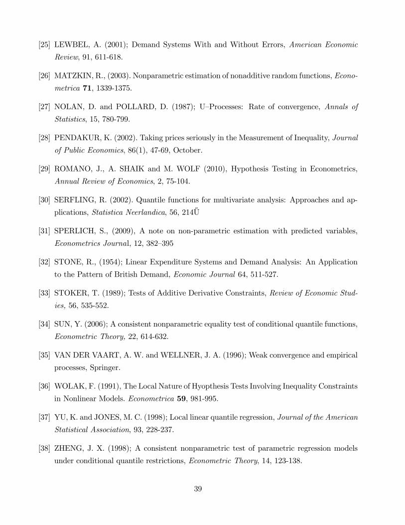
[25] LEWBEL, A. (2001); Demand Systems With and Without Errors, American Economic

Review, 91, 611-618.

[26] MATZKIN, R., (2003). Nonparametric estimation of nonadditive random functions, Econo-

metrica 71, 1339-1375.

[27] NOLAN, D. and POLLARD, D. (1987); U�Processes: Rate of convergence, Annals of

Statistics, 15, 780-799.

[28] PENDAKUR, K. (2002). Taking prices seriously in the Measurement of Inequality, Journal

of Public Economics, 86(1), 47-69, October.

[29] ROMANO, J., A. SHAIK and M. WOLF (2010), Hypothesis Testing in Econometrics,

Annual Review of Economics, 2, 75-104.

[30] SERFLING, R. (2002). Quantile functions for multivariate analysis: Approaches and ap-

plications, Statistica Neerlandica, 56, 214½U

[31] SPERLICH, S., (2009), A note on non-parametric estimation with predicted variables,

Econometrics Journal, 12, 382�395

[32] STONE, R., (1954); Linear Expenditure Systems and Demand Analysis: An Application

to the Pattern of British Demand, Economic Journal 64, 511-527.

[33] STOKER, T. (1989); Tests of Additive Derivative Constraints, Review of Economic Stud-

ies, 56, 535-552.

[34] SUN, Y. (2006); A consistent nonparametric equality test of conditional quantile functions,

Econometric Theory, 22, 614-632.

[35] VAN DER VAART, A. W. and WELLNER, J. A. (1996); Weak convergence and empirical

processes, Springer.

[36] WOLAK, F. (1991), The Local Nature of Hyopthesis Tests Involving Inequality Constraints

in Nonlinear Models. Econometrica 59, 981-995.

[37] YU, K. and JONES, M. C. (1998); Local linear quantile regression, Journal of the American

Statistical Association, 93, 228-237.

[38] ZHENG, J. X. (1998); A consistent nonparametric test of parametric regression models

under conditional quantile restrictions, Econometric Theory, 14, 123-138.

39

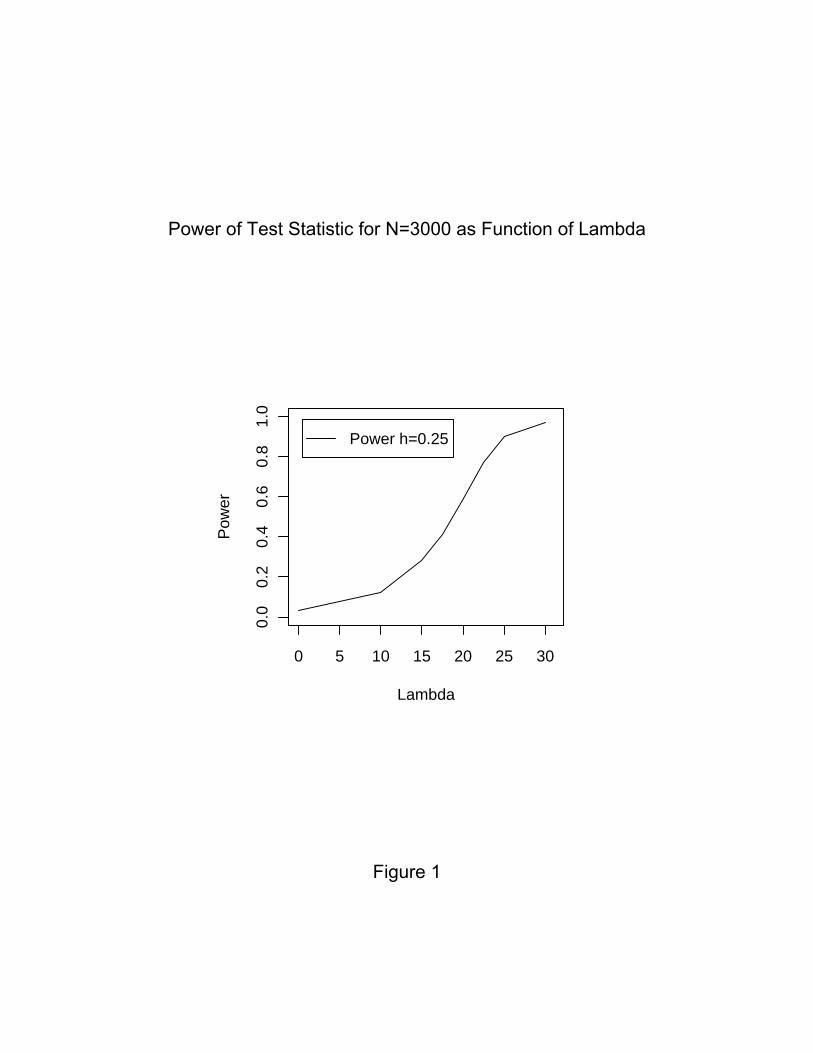
0 5 10 15 20 25 30

0.0

0.2

0.4

0.6

0.8

1.0

Lambda

Pow

er

Power h=0.25

Power of Test Statistic for N=3000 as Function of Lambda

Figure 1

0.0 0.2 0.4 0.6 0.8 1.0

0.0

0.2

0.4

0.6

0.8

1.0

Proportion Nonrational

Pow

er

Power h=0.25

Power of Test Statistic as Function of Proportion Nonrational Individuals

Figure 2

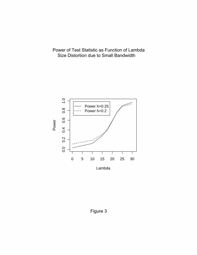
0 5 10 15 20 25 30

0.0

0.2

0.4

0.6

0.8

1.0

Lambda

Pow

er

Power h=0.25Power h=0.2

Power of Test Statistic as Function of Lambda Size Distortion due to Small Bandwidth

Figure 3

0 5 10 15 20 25 30

0.0

0.2

0.4

0.6

0.8

1.0

Lambda

Pow

er

n=1500n=3000n=6000

Power of Test Statistic as Function of Lambda Effect of Sample Size - Consistency of Test

Figure 4

0 5 10 15 20 25 30 35

0.0

0.2

0.4

0.6

0.8

1.0

Lambda

Pow

er

Normal Price VariationLimited Price Variation

Power of Test Statistic as Function of Lambda Influence of Effective Sample Size

Figure 5