The Influence of Meteorological Conditions onthe Icing Performance Penalties on a UAV Airfoil

Master’s thesisby

Nicolas Fajt

Institute of Aerodynamics and Gas Dynamicsof the University of Stuttgart

&Department of Engineering Cybernetics

of the Norwegian University of Science and Technology.

Stuttgart, July 2019

Erklarung

Hiermit versichere ich, dass ich diese Masterarbeit selbststandig mit Unterstutzung des Betreuers /der Betreuer angefertigt und keine anderen als die angegebenen Quellen und Hilfsmittel verwendethabe.Die Arbeit oder wesentliche Bestandteile davon sind weder an dieser noch an einer anderen Bil-dungseinrichtung bereits zur Erlangung eines Abschlusses eingereicht worden.Ich erklare weiterhin, bei der Erstellung der Arbeit die einschlagigen Bestimmungen zum Urheber-schutz fremder Beitrage entsprechend den Regeln guter wissenschaftlicher Praxis 1 eingehalten zuhaben. Soweit meine Arbeit fremde Beitrage (z.B. Bilder, Zeichnungen, Textpassagen etc.) enthalt,habe ich diese Beitrage als solche gekennzeichnet (Zitat, Quellenangabe) und eventuell erforderlichgewordene Zustimmungen der Urheber zur Nutzung dieser Beitrage in meiner Arbeit eingeholt. Mirist bekannt, dass ich im Falle einer schuldhaften Verletzung dieser Pflichten die daraus entstehendenKonsequenzen zu tragen habe.

Ort, Datum, Unterschrift

Betreuer: Dr.-Ing. Thorsten Lutz

Externer Betreuer: Dipl.-Ing. Richard Hann

1Nachzulesen in den DFG-Empfehlungen zur”Sicherung guter wissenschaftlicher Praxis“ bzw. in der Satzung der

Universitat Stuttgart zur”Sicherung der Integritat wissenschaftlicher Praxis und zum Umgang mit Fehlverhalten

in der Wissenschaft“

v

Contents

Scope iii

Statutory declaration vi

Contents vii

Symbols and abbreviations ix

List of figures xi

Abstract xii

Kurzfassung xiv

1 Introduction 1

2 Aircraft and UAV icing in general 32.1 Icing process . . . . . . . . . . . . . . . . . . . . . . . . . . . . . . . . . . . . . . . . 32.2 UAV icing vs. manned aircraft icing . . . . . . . . . . . . . . . . . . . . . . . . . . . 5

3 Methods 73.1 FENSAP-ICE . . . . . . . . . . . . . . . . . . . . . . . . . . . . . . . . . . . . . . . . 7

3.1.1 FENSAP . . . . . . . . . . . . . . . . . . . . . . . . . . . . . . . . . . . . . . 83.1.2 Turbulence models . . . . . . . . . . . . . . . . . . . . . . . . . . . . . . . . . 103.1.3 DROP3D . . . . . . . . . . . . . . . . . . . . . . . . . . . . . . . . . . . . . . 113.1.4 ICE3D . . . . . . . . . . . . . . . . . . . . . . . . . . . . . . . . . . . . . . . . 12

3.2 Grid setup . . . . . . . . . . . . . . . . . . . . . . . . . . . . . . . . . . . . . . . . . . 133.2.1 RG-15 airfoil . . . . . . . . . . . . . . . . . . . . . . . . . . . . . . . . . . . . 133.2.2 Generation of the numerical grids . . . . . . . . . . . . . . . . . . . . . . . . . 14

3.3 Grid dependency study . . . . . . . . . . . . . . . . . . . . . . . . . . . . . . . . . . 173.4 Meteorological icing conditions . . . . . . . . . . . . . . . . . . . . . . . . . . . . . . 18

4 Simulation models and validation 214.1 Clean airfoil performance model . . . . . . . . . . . . . . . . . . . . . . . . . . . . . . 21

4.1.1 Grid dependency study . . . . . . . . . . . . . . . . . . . . . . . . . . . . . . 214.1.2 Performance validation . . . . . . . . . . . . . . . . . . . . . . . . . . . . . . . 22

4.2 Iced airfoil performance model . . . . . . . . . . . . . . . . . . . . . . . . . . . . . . 244.2.1 Grid dependency study . . . . . . . . . . . . . . . . . . . . . . . . . . . . . . 244.2.2 Performance validation . . . . . . . . . . . . . . . . . . . . . . . . . . . . . . . 25

4.3 Ice accretion model . . . . . . . . . . . . . . . . . . . . . . . . . . . . . . . . . . . . . 274.3.1 Time-step study . . . . . . . . . . . . . . . . . . . . . . . . . . . . . . . . . . 284.3.2 Ice accretion validation . . . . . . . . . . . . . . . . . . . . . . . . . . . . . . 30

vii

Contents

5 Ice accretion results and performance degradation 335.1 Ice accretion . . . . . . . . . . . . . . . . . . . . . . . . . . . . . . . . . . . . . . . . . 335.2 Performance degradation . . . . . . . . . . . . . . . . . . . . . . . . . . . . . . . . . . 38

5.2.1 Lift, drag and pitching moment coefficient . . . . . . . . . . . . . . . . . . . . 385.2.2 Index visualization . . . . . . . . . . . . . . . . . . . . . . . . . . . . . . . . . 44

5.3 Uncertainties and future work . . . . . . . . . . . . . . . . . . . . . . . . . . . . . . . 465.4 Relevance of the simulation results for an IPS development . . . . . . . . . . . . . . 48

6 Conclusion 49

Bibliography 53

viii

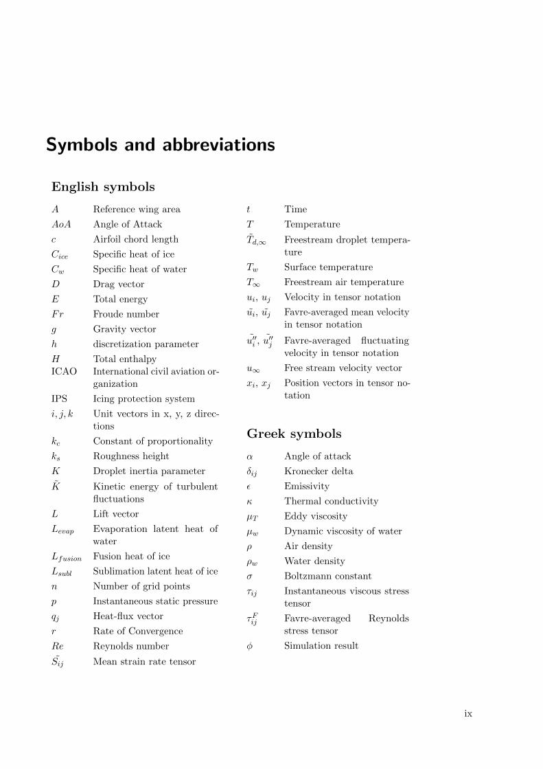
Symbols and abbreviations

English symbols

A Reference wing area

AoA Angle of Attack

c Airfoil chord length

Cice Specific heat of ice

Cw Specific heat of water

D Drag vector

E Total energy

Fr Froude number

g Gravity vector

h discretization parameter

H Total enthalpyICAO International civil aviation or-

ganization

IPS Icing protection system

i, j, k Unit vectors in x, y, z direc-tions

kc Constant of proportionality

ks Roughness height

K Droplet inertia parameter

K Kinetic energy of turbulentfluctuations

L Lift vector

Levap Evaporation latent heat ofwater

Lfusion Fusion heat of ice

Lsubl Sublimation latent heat of ice

n Number of grid points

p Instantaneous static pressure

qj Heat-flux vector

r Rate of Convergence

Re Reynolds number

Sij Mean strain rate tensor

t Time

T Temperature

Td,∞ Freestream droplet tempera-ture

Tw Surface temperature

T∞ Freestream air temperature

ui, uj Velocity in tensor notation

ui, uj Favre-averaged mean velocityin tensor notation

u′′i , u′′j Favre-averaged fluctuating

velocity in tensor notation

u∞ Free stream velocity vector

xi, xj Position vectors in tensor no-tation

Greek symbols

α Angle of attack

δij Kronecker delta

ε Emissivity

κ Thermal conductivity

µT Eddy viscosity

µw Dynamic viscosity of water

ρ Air density

ρw Water density

σ Boltzmann constant

τij Instantaneous viscous stresstensor

τFij Favre-averaged Reynoldsstress tensor

φ Simulation result

ix

List of figures

2.1 Droplet trajectory past an airfoil, image by L. Battisti [2]. . . . . . . . . . . . . . . . 3

2.2 Ice formations on a UAV airfoil, images by courtesy of Richard Hann. . . . . . . . . 4

2.3 Horn formation an a leading edge, image by NASA [31]. . . . . . . . . . . . . . . . . 5

3.1 Linked modules of ANSYS FENSAP-ICE, from [6]. . . . . . . . . . . . . . . . . . . . 7

3.2 Heat and mass transfer phenomena considered by ICE3D [24]. . . . . . . . . . . . . . 12

3.3 2D cross-section of the RG-15 airfoil. . . . . . . . . . . . . . . . . . . . . . . . . . . . 14

3.4 RG-15 grid setup for the (a), (c) performance grid and the (b), (d) ice accretion grid. 15

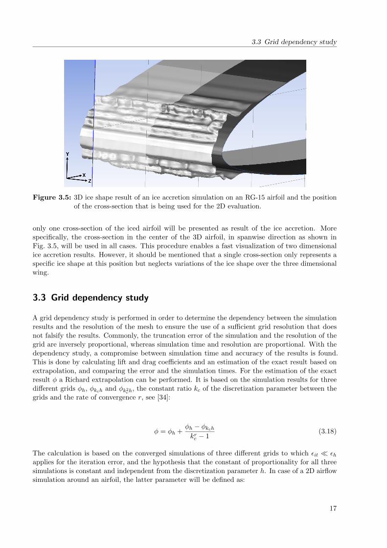
3.5 3D ice shape result of an ice accretion simulation on an RG-15 airfoil and the positionof the cross-section that is being used for the 2D evaluation. . . . . . . . . . . . . . . 17

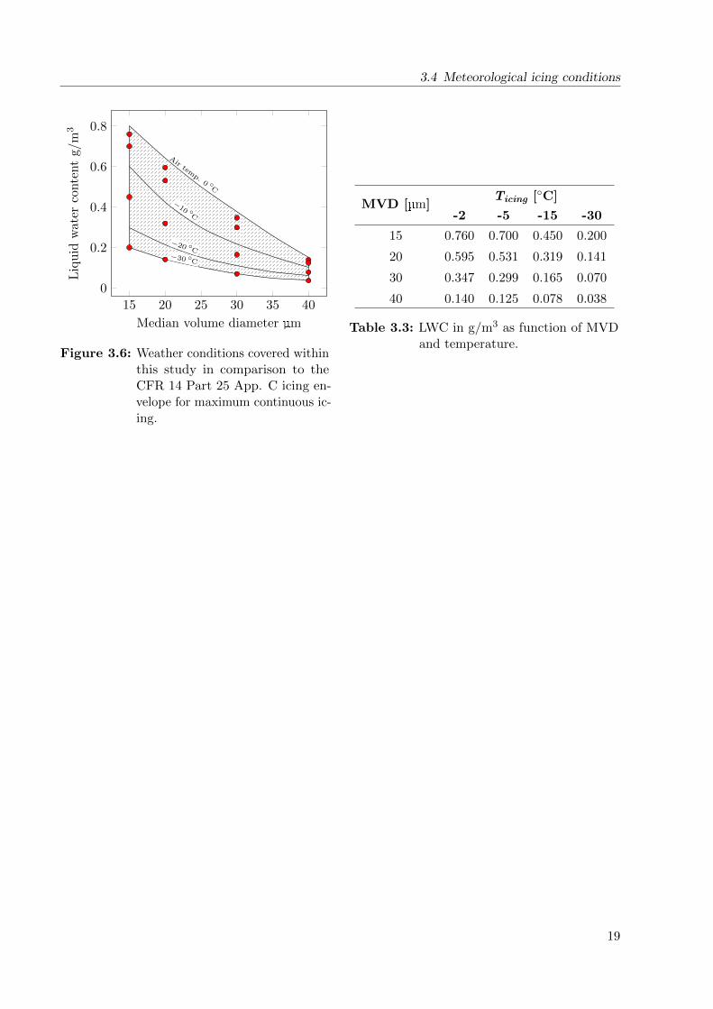
3.6 Weather conditions covered within this study in comparison to the CFR 14 Part 25App. C icing envelope for maximum continuous icing. . . . . . . . . . . . . . . . . . 19

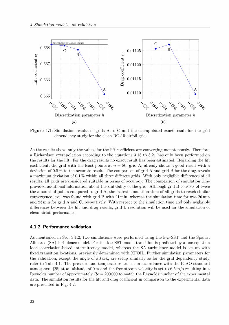
4.1 Simulation results of grids A to C and the extrapolated exact result for the griddependency study for the clean RG-15 airfoil grid. . . . . . . . . . . . . . . . . . . . 22

4.2 (a) Lift and (b) drag results for the clean RG-15 airfoil performance compared to theexperimental data, Re = 200 000. . . . . . . . . . . . . . . . . . . . . . . . . . . . . . 23

4.3 Numerical grid for the iced S826 airfoil performance simulation. . . . . . . . . . . . . 24

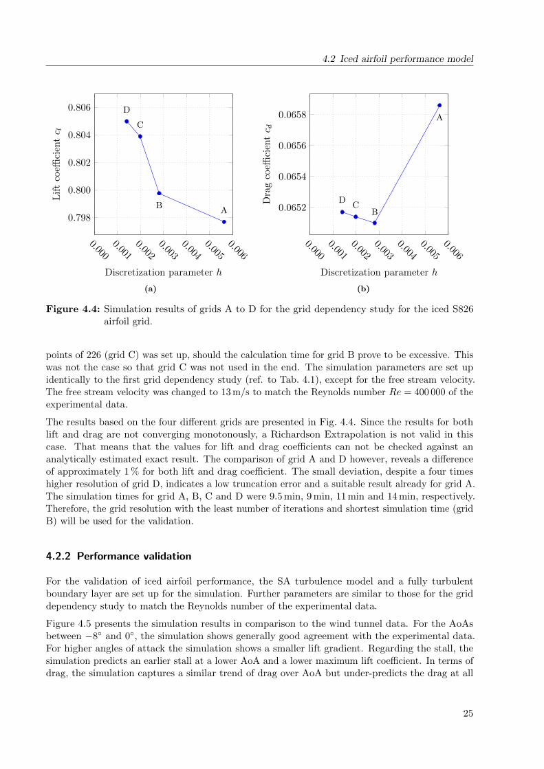
4.4 Simulation results of grids A to D for the grid dependency study for the iced S826airfoil grid. . . . . . . . . . . . . . . . . . . . . . . . . . . . . . . . . . . . . . . . . . 25

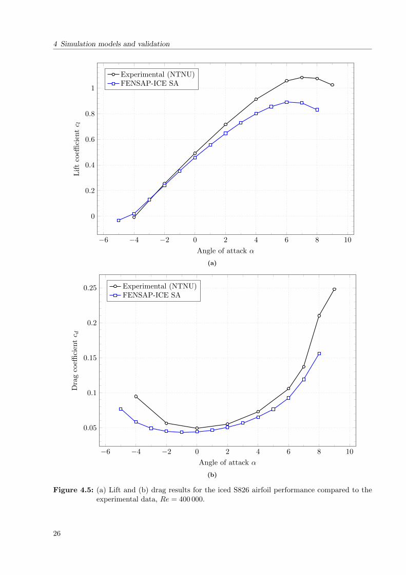
4.5 (a) Lift and (b) drag results for the iced S826 airfoil performance compared to theexperimental data, Re = 400 000. . . . . . . . . . . . . . . . . . . . . . . . . . . . . . 26

4.6 Large flow separation at the leading edge of the iced S826 NREL airfoil, AoA 5◦ andRe = 400 000. . . . . . . . . . . . . . . . . . . . . . . . . . . . . . . . . . . . . . . . . 27

4.7 Time-step study results for a (a) rime ice and (b) glaze ice case on the RG-15 airfoil. 29

4.8 Simulation results for the ice accretion at a (a) rime ice and (b) glaze ice case on theRG-15 airfoil, compared to wind tunnel results. . . . . . . . . . . . . . . . . . . . . . 30

4.9 Comparison of two RG-15 ice accretion simulations at identical icing conditions. . . 31

5.1 Ice shape results on the RG-15 for droplet sizes (a) 15 µm, (b) 20 µm, (c) 30 µm and(d) 40 µm at Re = 800 000 (at −2 ◦C) to 1 000 000 (at −30 ◦C). . . . . . . . . . . . . 35

5.2 Simulation results for the accumulated ice masses on the RG-15. . . . . . . . . . . . 36

5.3 Roughness height of the iced RG-15 airfoils. . . . . . . . . . . . . . . . . . . . . . . . 37

5.4 Lift coefficients of the iced RG-15 airfoils for the droplet sizes (a) 15 µm, (b) 20 µm,(c) 30 µm and (d) 40 µm at Re = 800 000. . . . . . . . . . . . . . . . . . . . . . . . . 39

5.5 Drag coefficients of the iced RG-15 airfoils for the droplet sizes (a) 15 µm, (b) 20 µm,(c) 30 µm and (d) 40 µm at Re = 800 000. . . . . . . . . . . . . . . . . . . . . . . . . 40

5.6 Airflow around the RG-15 leading edge at an AoA of 2◦ for (a) the clean airfoil, (b)the −30 ◦C / MVD 20 icing condition, (c) the −2 ◦C / MVD 20 icing condition and(d) the −2 ◦C / MVD 20 icing condition at an AoA of 6◦. . . . . . . . . . . . . . . . 41

xi

List of figures

5.7 Pressure distribution on the RG-15 at various angles of attack for (a) the clean airfoil,(b) the icing condition −30 ◦C / MVD 40, (c) −2 ◦C / MVD 20 and (d) a comparisonof (a) and (b) at the AoAs 8◦ and 12◦. . . . . . . . . . . . . . . . . . . . . . . . . . . 42

5.8 Moment coefficients of the iced RG-15 airfoils for the droplet sizes (a) 15 µm, (b)20 µm, (c) 30 µm and (d) 40 µm at Re = 800 000. . . . . . . . . . . . . . . . . . . . . 44

5.9 Index visualization of the RG-15 airfoil performance degradation for (a) lift, (b) drag,(c) moment coefficient and (d) stall angle. . . . . . . . . . . . . . . . . . . . . . . . . 46

xii

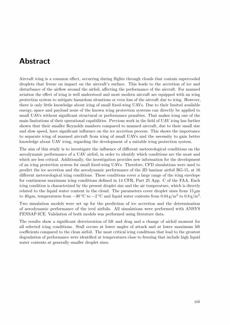
Abstract

Aircraft icing is a common effect, occurring during flights through clouds that contain supercooleddroplets that freeze on impact on the aircraft’s surface. This leads to the accretion of ice anddisturbance of the airflow around the airfoil, affecting the performance of the aircraft. For mannedaviation the effect of icing is well understood and most modern aircraft are equipped with an icingprotection system to mitigate hazardous situations or even loss of the aircraft due to icing. However,there is only little knowledge about icing of small fixed-wing UAVs. Due to their limited availableenergy, space and payload none of the known icing protection systems can directly be applied tosmall UAVs without significant structural or performance penalties. That makes icing one of themain limitations of their operational capabilities. Previous work in the field of UAV icing has furthershown that their smaller Reynolds numbers compared to manned aircraft, due to their small sizeand slow speed, have significant influence on the ice accretion process. This shows the importanceto separate icing of manned aircraft from icing of small UAVs and the necessity to gain betterknowledge about UAV icing, regarding the development of a suitable icing protection system.

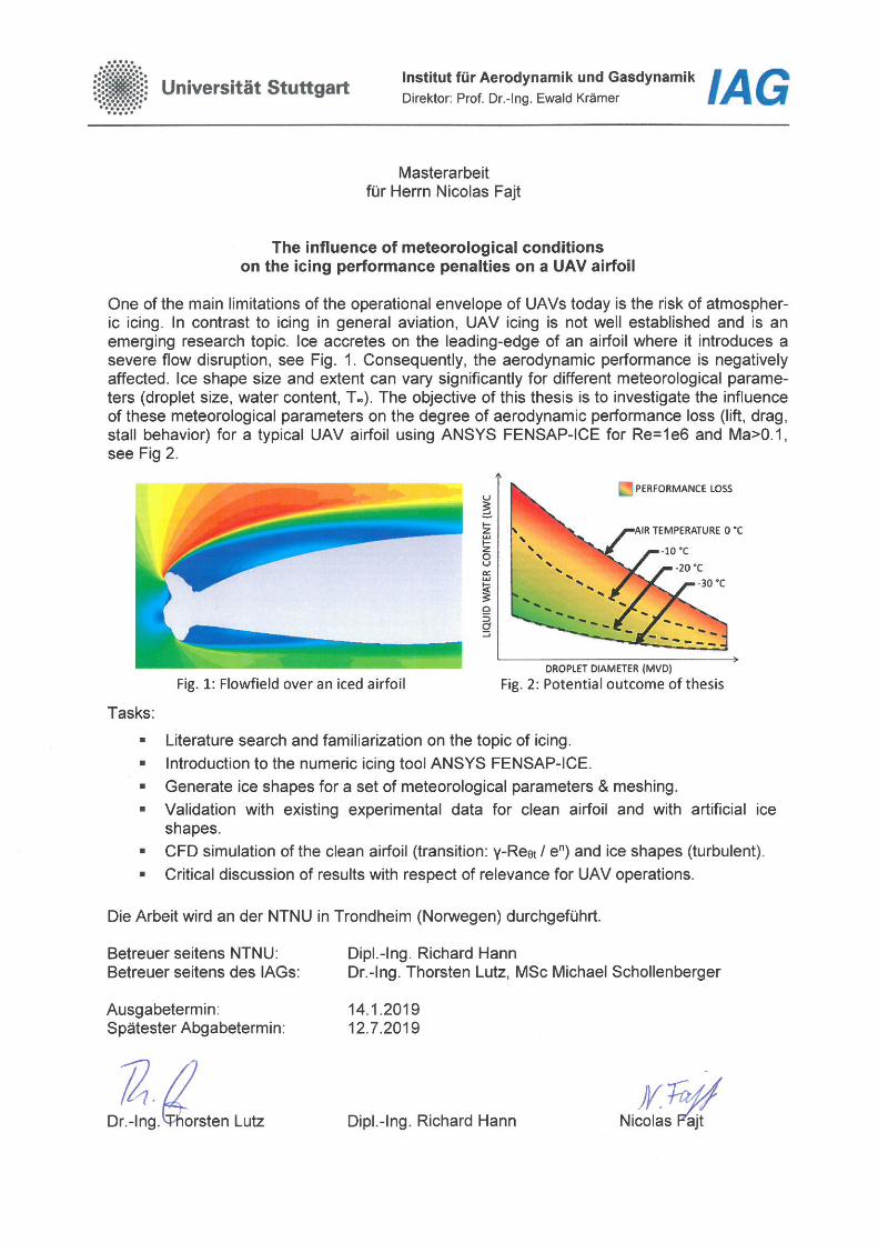
The aim of this study is to investigate the influence of different meteorological conditions on theaerodynamic performance of a UAV airfoil, in order to identify which conditions are the most andwhich are less critical. Additionally, the investigation provides new information for the developmentof an icing protection system for small fixed-wing UAVs. Therefore, CFD simulations were used topredict the ice accretion and the aerodynamic performance of the 2D laminar airfoil RG-15, at 16different meteorological icing conditions. These conditions cover a large range of the icing envelopefor continuous maximum icing conditions defined in 14 CFR, Part 25 App. C of the FAA. Eachicing condition is characterized by the present droplet size and the air temperature, which is directlyrelated to the liquid water content in the cloud. The parameters cover droplet sizes from 15 µmto 40 µm, temperatures from −30 ◦C to −2 ◦C and liquid water contents from 0.04 g/m3 to 0.8 g/m3.

Two simulation models were set up for the prediction of ice accretion and the determinationof aerodynamic performance of the iced airfoils. All simulations were performed with ANSYSFENSAP-ICE. Validation of both models was performed using literature data.

The results show a significant deterioration of lift and drag and a change of airfoil moment forall selected icing conditions. Stall occurs at lower angles of attack and at lower maximum liftcoefficients compared to the clean airfoil. The most critical icing conditions that lead to the greatestdegradation of performance were identified at temperatures close to freezing that include high liquidwater contents at generally smaller droplet sizes.

xiii

Kurzfassung

Flugzeugvereisung ist ein Effekt, der bei Flugen durch Wolken auftreten kann. Befinden sichunterkuhlte Wassertropfen in der Wolke, gefrieren diese beim Auftreffen auf der Oberflache desFlugzeuges. Dadurch lagert sich Eis an, welches die Umstromung des Flugels stort und dadurch dieaerodynamischen Eigenschaften des Tragflugelprofils verandert. Im Bereich der bemannten Luft-fahrt ist Vereisung umfangreich erforscht und die meisten modernen Flugzeuge sind mit Systemenausgestattet, welche Vereisung entweder verhindern oder eine Enteisung ermoglichen. Dadurchwerden kritische Flugsituationen verhindert, die aufgrund veranderter Flugzeugaerodynamik zumVerlust des Flugzeugs fuhren konnen. Vereisung unbemannter Flugzeugen, mit wenigen MeternSpannweite, ist hingegen deutlich weniger erforscht. Bisherige Forschungsergebnisse auf diesemGebiet haben gezeigt, dass vorhandenes Wissen und Systeme zum Vereisungsschutz nicht direktaus der bemannten Luftfahrt auf kleine unbemannte Flugzeuge angewandt werden konnen. Grundhierfur ist, dass die Reynoldszahl einen signifikanten Einfluss auf den Vereisungsprozess hat undbei Drohnen, aufgrund der geringeren Spannweite und langsameren Fluggeschwindigkeit, kleinereReynoldszahlen vorherrschen. Bedingt durch die geringe Große, begrenzte Nutzlast und begrenzteelektrische Energie von Drohnen, konnen bekannte Systeme nicht direkt aus der bemannten Luftfahrtubernommen werden. Daher ist es wichtig Vereisungsvorgange an kleinen, unbemannten Flugzeugenvon der Vereisung bemannter Flugzeuge zu unterscheiden und im Hinblick auf die Entwicklungvon Systemen zum Vereisungsschutz, weiterfuhrende Untersuchungen im Bereich der Drohnen-vereisung durchzufuhren. Das Ziel dieser Arbeit ist, den Einfluss verschiedener Wetterbedingungenauf die aerodynamischen Eigenschaften eines Tragflugelprofils einer Drohne zu bestimmen. DieUntersuchung sollte zeigen, welche Wetterbedingungen kritischen Einfluss auf die Aerodynamik derProfils haben und welche weniger großen Einfluss haben. Die Ergebnisse sollen neue Erkenntniseliefern, die fur die Entwicklung eines Systems zum Vereisungsschutz genutzt werden konnen. Furdie Umsetzung dieser Ziele wurden CFD Simulationen durchgefuhrt, um die Eisanlagerung und dieaerodynamischen Eigenschaften des 2D-Laminarprofils RG-15, unter 16 verschiedenen Wetterbedin-gungen, zu untersuchen. Diese Wetterbedingungen decken einen Großteil der Vereisungsbedingungender FAA Regularien fur maximum continuous icing der 14 CFR Part 25 App. C ab und sinddefiniert anhand der Tropfengroße, der Umgebungstemperatur und dem Wassergehalt in der Wolke.Die ausgewahlten Wetterbedingungen umfassen Tropfengroßen von 15 µm bis 40 µm, Temperaturenvon −30 ◦C bis −2 ◦C und einen Wassergehalt zwischen 0.04 g/m3 und 0.8 g/m3.

Insgesamt wurden zwei Simulationsmodelle genutzt, eines fur die Eisanlagerung und eines um dieaerodynamischen Eigenschaften der vereisten Profile zu bestimmen. Fur alle Simulationen wurdeANSYS FENSAP-ICE genutzt. Zur Validierung beider Modelle wurden experimentelle Daten ausder Literatur herangezogen.

Die Ergebnisse zeigen eine Reduzierung des Auftriebs, einen Anstieg des Widerstandes und einenAnstieg des Momentengradienten, fur alle untersuchten Wetterbedingungen. Stromungsabriss trittbei kleineren Anstellwinkeln und geringerem maximalen Auftriebskoeffizienten auf. Die kritischstenVereisungsbedingungen wurden bei Temperaturen nahe dem Gefrierpunkt festgestellt, bei denender Wassergehalt in der Wolke am hochsten ist und kleine Tropfen vorherrschen.

xv

1 Introduction

Small, fixed-wing unmanned aerial vehicles (UAV) with a wingspan of approximately 2 to 4 m offerless costs, less risk and a high performance compared to manned aircraft. This makes them attractivefor many surveillance, reconnaissance and scientific research purposes, especially in life-hostile areaslike the Arctic. As UAVs are suitable for an increasing variety of activities the market has grown inthe last few years and the wider field of applications emerges the necessity to operate the UAVs inadverse weather conditions. One of the main limitations for safe flight in those weather conditions isicing of the aircraft. Ice accretion affects the weight of the aircraft, changes its center of gravity andresults in a degradation of aerodynamic performance due to decreasing lift and increasing drag [8].These influences can lead to hazardous flight situations. To counteract this, manned aircraft areequipped with sensors and icing protection systems to detect and remove ice. UAVs however lacksuch icing protection systems, mainly due to their smaller size in combination with less availableenergy. In addition, the generally lower airspeed and flight altitude exposes them to icing conditionsfor a longer period of time. At least in the past, the US Army’s approach was to avoid hazardousflight situations by not launching into known icing conditions [27]. This partially solves the problem,but also leads to large restrictions of operational capabilities.

Although the topic of icing was already known in 1990 [36], there was only little research done inthe field UAV icing. However, the frequent presence of icing conditions and the lack of effective icingprotection systems for small UAVs show the increasing importance to gain better understanding oficing of UAVs. Therefore, in the last years, further research on this topic has been conducted byseveral groups. Szilder and McIlwain have described the influence of UAV-typical low Reynoldsnumbers (Re = 1 − 10 · 105) on the ice accretion process [40], whereas regular manned aircraftconfigurations are characterised by higher Renolds numbers (Re = 1 − 10 · 106) [40]. Based oninvestigations using their morphogenetic icing model [39], they found that higher Reynolds numberslead to a reduction of rime and increase of glaze ice in a parametric space, defined by air temperatureand liquid water content. Rime and glaze ice are different ice shapes that occur at different icingtemperatures. Various ice shapes that can occur are presented in more detail in the subsequentCh. 2. Another major finding came from the investigation of ice shapes, when an airfoil travels thesame distance through icing conditions at various Reynolds numbers. In this comparison it wasimportant to note that the increase of the Reynolds number is associated with an increase in velocity,but a decrease of icing duration, which is inversely proportional to the velocity. This investigationconfirmed their first findings. At a Reynolds number of Re = 5 · 104 only rime ice formed. For aReynolds number of Re = 1 · 105 a co-existence of rime and glaze ice has been found and for furtherincreased Reynolds numbers of Re ≥ 5 · 105, only glaze ice formed. Besides those findings, moreimportantly, the results clearly showed significantly smaller ice extends at higher Reynolds numbers,although the overall ice mass increases with increasing Reynolds numbers. This implies, that icingof airfoils at lower Reynolds numbers could have a greater impact on the aerodynamics. The resultsof Szilder and McIlwain imply the importance to separate studies on the ice accretion process ofsmall-sized fixed-wing UAVs from general aircraft icing.

1

1 Introduction

Apart from their morphogenetic approach for an icing model other common tools to simulateicing of UAVs are the panel-method based NASA code LEWICE, used by Koenig et al. [26]and state-of-the-art computational fluid dynamics (CFD) icing code FENSAP-ICE, capable ofdetermining 2D and 3D ice accretion, used by Tran et al. [43]. A comparison between LEWICEand FENSAP-ICE has been covered by Hann [19] in order to assess the suitability of both codes topredict ice shapes and performance degradation. The comparison showed that both codes predict asignificant decrease of maximum lift, stall angle and increase of drag for three different investigatedicing cases rime, glaze and mixed ice. However, the comparison also revealed limitations of thepanel-method used within LEWICE. For the the rime ice case, which is the most streamlined icingform, both codes predict congruent ice shapes. For the mixed and glaze ice case however, bothcodes predict significantly deviating ice shapes. This in consequence, led to similar performanceresults of both codes for the rime ice case but discrepancies for the mixed and glaze ice case.

The above mentioned earlier work on UAV icing has shown that ice accretion affects the aerody-namic performance negatively, but no study has been conducted that investigates the relation ofmeteorological conditions to the degradation of performance. Therefore, the aim of this study is toinvestigate the influence of various meteorological conditions on the aerodynamic performance ofa UAV airfoil. To do so, a 2D airfoil RG-15 is being investigated under several icing conditions,by using CFD simulations. Regarding the development of effective and efficient icing protectionsystems (IPS) for UAVs it is crucial to identify worst case icing conditions. Additionally, theknowledge about the influence of different icing conditions on the airfoil’s performance is essentialfor the adaption of flight controllers, to enable safe flight in varying weather conditions and therebyextending the UAV’s operational capabilities.

2

2 Aircraft and UAV icing in general

This chapter is mainly intended to readers who are not familiar with the topic of aircraft icing. Itgives an introduction to the icing process in general and depicts the differences between UAV andmanned aircraft icing.

2.1 Icing process

Aircraft icing occurs during flights at a temperature near or below freezing through clouds thatcontain supercooled water droplets. The droplets impinge the aircraft’s surface and freeze. As aresult, geometry and surface roughness of the airfoil changes. The shape and amount of ice dependson the size and roughness of the surface, the speed of the aircraft, the air temperature, the surfacetemperature, the liquid water content in the cloud and the droplet size.

As described in [13], icing is usually divided into two forms, structural and induction icing. Structuralicing includes ice on all surfaces of an aircraft, whereas induction icing only refers to ice occurringin the engine’s induction system. This thesis focuses solely on structural icing on airfoils. Thesimulation of ice accretion can be separated, into two different steps.

The first step is to determine the quantity of water impinging on the surface of the airfoil. Therefore,the droplet trajectories around the airfoil are calculated [2]. Generally, the supercooled waterdroplets tend to follow the airflow streamlines in freestream conditions. If an obstacle like the airfoilapproaches, their paths diverge from the airflow streamlines, due to drag and inertia which arerelated to the size and mass of the droplets. As a result of the balance between initial velocity,drag and inertia the droplets either hit the surface or divert around the airfoil (see Fig. 2.1).The parameters that describe the distribution of water on the surface are the upper and lowerimpingement limits as well as the collection efficiency. These limits are the most aft points on theairfoil behind the stagnation point where droplets hit the surface. The collection efficiency describesthe fraction of water caught by a certain area of the airfoil in relation to the water content of thefreestream.

Figure 2.1: Droplet trajectory past an airfoil, image by L. Battisti [2].

3

2 Aircraft and UAV icing in general

(a) Rime Ice (b) Glaze Ice

Figure 2.2: Ice formations on a UAV airfoil, images by courtesy of Richard Hann.

The freezing process of the water is the second step. It is governed by parameters that affectthe thermal conduction between the airfoil’s surface and the impinging water, such as the surfaceroughness, the temperature and the speed of the aircraft. Ice increases the surface roughnesscompared to the un-iced airfoil. This enhances the convective heat transfer, which cools down thesurface even further and increases ice accretion [2]. Besides thermodynamic mechanisms, the timethat takes the droplets to freeze on the surface is decisive for the final ice shape. The three mostcommon ice forms are rime, glaze and mixed ice. The different icing forms are described by R. W.Gent et al. in [15], the FAA in [13] and L. Battisti in [2].

Rime ice has an opaque and relatively streamlined shape with a rough surface (see Fig. 2.2a). Itoccurs at low temperatures of about −15 ◦C to −30 ◦C, low speeds and less LWCs when the dropletsfreeze rapidly on impact. The typically opaque appearance is caused by air trapped between thefrozen droplets.

Glaze ice appears at temperatures close to the freezing point (approximately−1 ◦C to−5 ◦C), higherspeeds and high LWCs, when the droplets don’t freeze completely on impact. It is characterized bya more transparent appearance and a smoother surface compared to rime ice (see Fig. 2.2b). It alsoexhibits the strongest adhesion to the surface, compared to other icing forms. Glaze ice can lead todangerous ice formations, when the water is running back on the surface and freezes behind thearea covered by de-icing systems.

Mixed ice, the third ice shape is, a combination of rime and glaze ice. During a flight in icingconditions, speed of the aircraft, temperature, droplet size and water content of the clouds vary,creating an ice shape with characteristics of both rime and glaze ice. In many cases, rime ice canbe found near the stagnation point of the airfoil, where the water freezes immediately. Furtherdownstream the ice gets more transparent and smooth, caused by water that ran back and freezeson the surface. From an aerodynamic point of view, mixed ice can be considered the most severeicing form, since it tends to build the largest protuberances, in literature often described as “glazehorns” [2]. Those horns build up from the stagnation point against the airflow in an approximately45◦ angle (see Fig. 2.3) and result in detachment of the airflow and significant increase of drag.

4

2.2 UAV icing vs. manned aircraft icing

Figure 2.3: Horn formation an a leading edge, image by NASA [31].

2.2 UAV icing vs. manned aircraft icing

Manned aircraft use a variety of de-icing systems to protect the airfoil from ice accretion basedon three different methods, presented in [42] by S. K. Thomas. Those methods are either usingfreezing point depressants, thermal melting or surface deformation.

1. Freezing point depressants are chemical fluids (typically ethylene glycol) which are storedin the aircraft and can be pumped onto the wing through small nozzles during flight to preventwater from freezing on the surface and de-ice already frozen water. A main advantage of thissystem is the low power demand for the operation. For example the Air Force Predator, aUAV with 14.65 m wingspan (see [27]) is equipped with such a system. Another advantage isthat during operation state of the system no water that runs further back on the airfoil freezesto the surface. On the downside, the system significantly adds weight to the aircraft. Notonly the pumps, tubes and nozzles but also the tank and the liquid itself contribute to theweight gain. The tank volume further limits the maximum operation duration of the system.Lastly, the de-icing efficiency of the system decreases in weather conditions, that favor theadhesive bond between ice and the surface.

2. Thermal melting can be further divided into complete evaporation of the surface water(fully evaporative systems) and systems that melt the ice but allow water on the surface(running wet systems). Thermal melting systems which aim for a complete evaporation of icerequire more energy compared to the systems which allow water on the surface. To reducethe energy consumption, thermal systems can not only be operated continuously but alsointermittently. Depending on the available energy the system can be operated throughout thewhole flight, to avoid ice completely or it can be operated as de-icing system to remove icefrom the surface. In comparison to the freezing point depressant systems, thermal systemshave a constant mass and the operation duration is only limited by the available electricalpower. On the other hand, thermal systems can not prevent ice accretion by water that ranback on the surface to areas which aren’t covered by the icing protection system.

5

2 Aircraft and UAV icing in general

3. Surface deformation systems are only operating intermittently, allowing a certain amountof ice to form on the surface before being removed either by a pneumatic system with astretchable surface, which deforms when being pressurized or an electromagnetic impulse in theaircraft’s skin. The system’s design enables effective de-icing with lower power consumption,compared to thermal systems. Operation duration of this system is only limited by theavailable power. However, unlike the other two systems, deformation systems are unable toavoid icing in the first place. Also, these systems are unable to prevent icing in aft areasbehind the icing protection system.

The majority of small and medium sized UAVs don’t contain one of the above mentioned systems.Limiting factors are electrical power in order to increase their range, space availability and payloadrestrictions. Further, the necessity for fully autonomous icing detection systems is a major challengefor icing protection systems in UAVs. As of today, D·ICE from UBIQ Aerospace, an electro-thermalIPS, is the only commercially available icing protection system for unmanned aircrafts [1]. D·ICE isbased on nanotechnology and innovative electro-thermal design [22] that has been developed at theCentre of Autonomous Marine Operations and Systems (AMOS) at the Norwegian University ofScience and Technology (NTNU) in close collaboration with NASA Ames Research Center. Thesystem uses temperature sensors embedded in the surface of the aircraft and a specific controlalgorithm for a fully autonomous icing detection. The system was first introduced in [37] by Kim S.and a proof-of-concept study as well as experimental investigations of the system are publishedin [38] and [22].

The comparison to IPS systems for manned aircrafts, with currently only one system availablefor small-sized fixed-wing UAVs clearly shows the imperative to gain better understanding of theinfluence of various meteorological conditions, to be able to adapt flight controller and derive furtherinnovative icing protection systems for UAVs.

6

3 Methods

For the evaluation of performance degradation of an iced airfoil via CFD simulations, two differentsimulation models are used. One model is set up to capture the ice accretion on the airfoil for variousmeteorological conditions to generate the respective ice shapes. The setup of the second simulationmodel is based on the output geometry of the first model and will be used to acquire the aerodynamicperformance of the iced airfoils. This chapter gives an overview over the utilized numerical methodsof the simulation software, as well as their fluid mechanical principles. Subsequently, an introductionto the investigated airfoil, the setup of the different grids and the basics of a grid dependency studyare described. Lastly, all meteorological icing conditions that are covered in this study are presented.

3.1 FENSAP-ICE

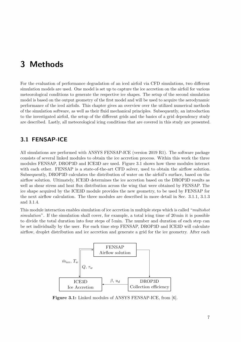
All simulations are performed with ANSYS FENSAP-ICE (version 2019 R1). The software packageconsists of several linked modules to obtain the ice accretion process. Within this work the threemodules FENSAP, DROP3D and ICE3D are used. Figure 3.1 shows how these modules interactwith each other. FENSAP is a state-of-the-art CFD solver, used to obtain the airflow solution.Subsequently, DROP3D calculates the distribution of water on the airfoil’s surface, based on theairflow solution. Ultimately, ICE3D determines the ice accretion based on the DROP3D results aswell as shear stress and heat flux distribution across the wing that were obtained by FENSAP. Theice shape acquired by the ICE3D module provides the new geometry, to be used by FENSAP forthe next airflow calculation. The three modules are described in more detail in Sec. 3.1.1, 3.1.3and 3.1.4.

This module interaction enables simulation of ice accretion in multiple steps which is called “multishotsimulation”. If the simulation shall cover, for example, a total icing time of 20 min it is possibleto divide the total duration into four steps of 5 min. The number and duration of each step canbe set individually by the user. For each time step FENSAP, DROP3D and ICE3D will calculateairflow, droplet distribution and ice accretion and generate a grid for the ice geometry. After each

FENSAPAirflow solution

ICE3DIce Accretion

DROP3DCollection efficiency

β, ud

Q, τw

mice, Tw

Figure 3.1: Linked modules of ANSYS FENSAP-ICE, from [6].

7

3 Methods

File Application

Custom remeshing.jou FLUENT – FENSAP interaction

Remeshing.jou Grid creation process

MeshingSizes.scm Grid control parameters

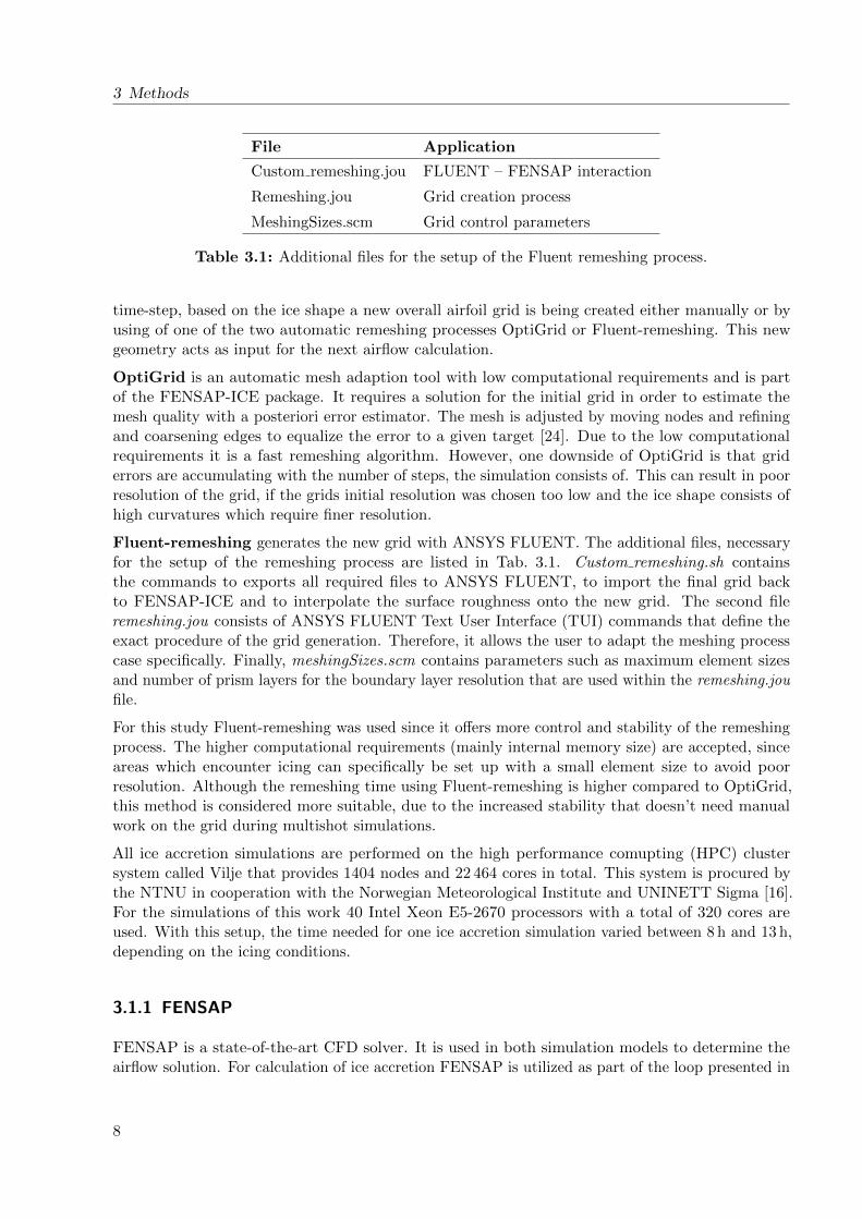
Table 3.1: Additional files for the setup of the Fluent remeshing process.

time-step, based on the ice shape a new overall airfoil grid is being created either manually or byusing of one of the two automatic remeshing processes OptiGrid or Fluent-remeshing. This newgeometry acts as input for the next airflow calculation.

OptiGrid is an automatic mesh adaption tool with low computational requirements and is partof the FENSAP-ICE package. It requires a solution for the initial grid in order to estimate themesh quality with a posteriori error estimator. The mesh is adjusted by moving nodes and refiningand coarsening edges to equalize the error to a given target [24]. Due to the low computationalrequirements it is a fast remeshing algorithm. However, one downside of OptiGrid is that griderrors are accumulating with the number of steps, the simulation consists of. This can result in poorresolution of the grid, if the grids initial resolution was chosen too low and the ice shape consists ofhigh curvatures which require finer resolution.

Fluent-remeshing generates the new grid with ANSYS FLUENT. The additional files, necessaryfor the setup of the remeshing process are listed in Tab. 3.1. Custom remeshing.sh containsthe commands to exports all required files to ANSYS FLUENT, to import the final grid backto FENSAP-ICE and to interpolate the surface roughness onto the new grid. The second fileremeshing.jou consists of ANSYS FLUENT Text User Interface (TUI) commands that define theexact procedure of the grid generation. Therefore, it allows the user to adapt the meshing processcase specifically. Finally, meshingSizes.scm contains parameters such as maximum element sizesand number of prism layers for the boundary layer resolution that are used within the remeshing.joufile.

For this study Fluent-remeshing was used since it offers more control and stability of the remeshingprocess. The higher computational requirements (mainly internal memory size) are accepted, sinceareas which encounter icing can specifically be set up with a small element size to avoid poorresolution. Although the remeshing time using Fluent-remeshing is higher compared to OptiGrid,this method is considered more suitable, due to the increased stability that doesn’t need manualwork on the grid during multishot simulations.

All ice accretion simulations are performed on the high performance comupting (HPC) clustersystem called Vilje that provides 1404 nodes and 22 464 cores in total. This system is procured bythe NTNU in cooperation with the Norwegian Meteorological Institute and UNINETT Sigma [16].For the simulations of this work 40 Intel Xeon E5-2670 processors with a total of 320 cores areused. With this setup, the time needed for one ice accretion simulation varied between 8 h and 13 h,depending on the icing conditions.

3.1.1 FENSAP

FENSAP is a state-of-the-art CFD solver. It is used in both simulation models to determine theairflow solution. For calculation of ice accretion FENSAP is utilized as part of the loop presented in

8

3.1 FENSAP-ICE

Fig. 3.1, whereas for simulating aerodynamic performance, FENSAP is used as stand-alone system.For all simulations a steady-state airflow solution is being determined. Spatial discretization iscarried out with a weak galerkin finite element method [30]. The nonlinear governing equations arelinearized by a Newton method where only one iteration at each time step is required when solvingfor a steady-state solution [3, 24].

Generally, FENSAP is capable of solving incompressible, compressible, steady, unsteady, viscousand inviscid three dimensional flows [18]. For incompressible flows FENSAP offers Euler equations,whereas for compressible flows FENSAP solves compressible Reynolds Averaged Navier-Stokes(RANS), also termed Favre-averaged Navier-Stokes equations. Since the latter equations are solvedfor the simulations within this work, the difference of Favre-averaged Navier-Stokes equations tofull Navier-Stokes equations for compressible flows will be explained.

With direct numerical simulations (DNS) the equations for conservation of mass, momentum andenergy are solved directly without any turbulence modeling [34]. The instantaneous equations areas follows:

∂ρ

∂t+

∂

∂xi(ρui) = 0 (3.1)

∂

∂t(ρui) +

∂

∂xj(ρujUj) = − ∂p

∂xi+∂τij∂xj

(3.2)

∂

∂t(ρE) +

∂

∂xj(ρujH) =

∂

∂xj(uiτij) +

∂

∂xj

(κ∂T

∂xj

)(3.3)

Directly solved means, the whole range of spatial and temporal scales of the turbulence must beresolved to capture the smallest dissipative scales. This requires extremely high resolutions of thecomputational mesh and extremely small time steps. As a consequence, the computational costsfor direct numerical simulations are very high, which makes them inappropriate for most practicalsimulations.

With Favre-averaged Navier-Stokes equations, the Navier-Stokes equations are solved in a time-and density-averaged form. Hence, turbulence is not directly resolved within these equations andneeds to be estimated by appropriate turbulence models. The use of this approach simplifies flowcalculation but is sufficient for most cases and requires less computational costs. In order to derivethe Favre-averaged Navier-Stokes equations from the ordinary Navier-Stokes equations all quantitiesof the equations are expressed as sum of mean and fluctuating parts [45]. Subsequently, density andpressure are being time-averaged, whereas the other parameters such as velocities, total internalenergy, enthalpy and temperature are being mass-averaged. The final Favre-averaged Navier-Stokesequations are as follows:

9

3 Methods

∂ρ

∂t+

∂

∂xi(ρui) = 0 (3.4)

∂

∂t(ρui) +

∂

∂xj(ρuj ui) = − ∂p

∂xi+

∂

∂xj

[τij − ρu′′ju′′i

](3.5)

∂

∂t

(ρE)

+∂

∂xj

(ρujH

)=

∂

∂xj

[ui

(τij − ρu′′i u′′j

)]+

∂

∂xj

[κ∂T

∂xj− ρu′′jh′′ + τiju′′i −

1

2ρu′′ju

′′i u′′i

] (3.6)

For the detailed derivation of the equations 3.4 to 3.6, see [45].

Equations 3.4, 3.5 and 3.6 only differ from the conventional Navier-Stokes equations (3.1, 3.2 and 3.3)by the appearance of the Favre-averaged Reynolds-stress tensor:

τFij = ρu′′i u′′j (3.7)

The turbulent heat flux ρu′′jh′′, the molecular diffusion τiju′′i and the turbulent transport 1

2 ρu′′ju′′i u′′i .

With molecular diffusion and turbulent transport often being neglected, the aim of a turbulencemodel is to postulate approximations for the six components of the Reynolds-stress tensor 3.7 andthe three components of the turbulent heat flux vector, to close the system of equations.

3.1.2 Turbulence models

The eddy viscosity concept, first introduced by Joseph Valentin Boussinesq, offers a suitablegeneralization for turbulent stresses of compressible flow, in the following form (see also [45]):

τFij = −ρu′′i u′′j = 2µT

(Sij −

1

3

∂uk∂xk

δij

)− 2

3ρKδij (3.8)

In many cases, the contribution of the last term, the turbulent kinetic energy, is ignored [45].

A commonly used closure approximation for the heat flux vector is based on the classical Reynoldsanalogy:

ρu′′jh′′ = −µT cp

PrT

∂T

∂xj(3.9)

The concept of eddy viscosity and the Reynolds analogy for the closure approximation of theFavre-averaged Reynolds-stress tensor and the turbulent heat-flux vector respectively reduces thenumber of unknowns to one, the eddy viscosity µT . Turbulence models based on this approximationare therefore categorized as linear eddy viscosity models. The models can be further divided intoone-equation and two-equation models, depending on the applied number of transport equations to

10

3.1 FENSAP-ICE

determine µT . FENSAP-ICE offers three different eddy viscosity models. Below, the two differentturbulence models used within this work are presented, pointing out their advantages, disadvantagesand their scope within this study. For reasons of clarity, the implemented transport equations ofeach model will not be presented here. These equations and a detailed listing and description oftheir coefficients can be found in the FENSAP-ICE User Manual [24].

The Spalart-Allmaras is a one-equation model that offers a high numerical stability and goodresults for attached flows but also cases in which flow separation can occur. Previous work by Hannet al. [23] has shown that the SA model performs best on clean airfoils in combination with fixedtransition locations. Therefore, the SA model with fixed transition is applied for the performancesimulations of the clean airfoil. This includes the clean airfoil simulation for the validation of theperformance model. All clean airfoil simulations using the SA model with fixed transition obtainthe transition location from XFOIL [10]. For the performance simulation of iced airfoils the SAmodel is also the preferred choice, since the work by Hann et al. [23] revealed generally highercomputational stability of the SA model compared to the k-ω-SST model.

However, simulations including ice, such as ice accretion and iced airfoil performance, are set upfully turbulent with the SA model. The reason for the fully turbulent setup is because an immediatetransition from laminar to turbulent boundary layer is expected at the iced leading edge, due to theincreased surface roughness and changed airfoil geometry.

Due to the good results obtained with this turbulence model in previous work and its high stability,the SA model is the main turbulence model used for the simulations of this study.

The k-ω-SST turbulence model uses two transport equations and a blending function. The idea ofthis model in general is, to combine the good results of the k-ε model in free stream conditions andthe good results of the k-ω model for flows near walls. This is done by using a step function to switchbetween these to models, where the k-ε transport equations are used outside the boundary layer,and the k-ω transport equations inside the boundary layer (see [24]). One additional simulationwith the k-ω-SST is set up for the validation of the clean airfoil performance, to find the differencesof the two turbulence models.

3.1.3 DROP3D

DROP3D is the Eulerian droplet impingement module. It calculates the mass of water captured bythe airfoil and the droplet impingement limits [5]. The mathematical model has been introduced byBourgault et al. [7]. It is essentially a two-fluid model that consists of the Navier-Stokes or Eulerequations for viscous and inviscid air, augmented by two droplet-specific continuity and momentumequations [30]. In non-dimensional form these equations are:

∂α

∂t+∇ · (αud) = 0 (3.10)

∂ud∂t

+ ud · ∇ud =cd dropletRed

24K(ua − ud) +

(1− ρ

ρw

)1

Fr2g (3.11)

where ua is the air velocity, the two variables α and ud are mean values of the water volume fractionand the droplet velocity, respectively, K is the droplet inertia parameter, Fr the Froude number andρw the water density. The right-hand-side terms of equation 3.11 represents the air drag force onthe droplets and the buoyancy and gravity forces. The air velocity ua is obtained by the FENSAP.

11

3 Methods

Figure 3.2: Heat and mass transfer phenomena considered by ICE3D [24].

The droplets are assumed to be spherical and of single and uniform size, equal to the median volumediameter. Within this model, no collision or mixing between the droplets is accounted for since it hasproven not to be important for icing situations. The droplets drag coefficient cd droplet is determinedby an empirical relation based on the droplet Reynolds number Red [3]. According to [30], thespherical droplet approximation is valid for droplet Reynolds numbers below 500. Since dropletsstart to deform already at droplet Reynolds numbers above 250 two additional drag correlationsfor determining the droplet drag coefficient are implemented in DROP3D. Within this work onlyspherical assumption is used. For all detailed drag correlations see [24]. Further, the effect ofdroplets on the airflow is neglected because of the low liquid water concentration. Thus, airflow canbe determined before solving the droplet-specific continuity and momentum equations.

Finally, a finite element Galerkin formulation is used to numerically discretize the equations, with astreamline upwinding Petrov-Galerkin (SUPG) term added. More details of the numerical methodand validations can be found in [5].

3.1.4 ICE3D

ICE3D is the ice accretion module. It calculates the ice accretion rate based on the friction forceand the heat fluxes obtained by FENSAP and the mass rate of water caught known from theimpingement module DROP3D [6].

The equilibrium model is based on a partial differential equation system of conservation equationsand was introduced in [4]. It is derived based on the Messinger model [28] and further improved topredict the ice accretion and water runback on the surface. The heat and mass transfer phenomenataken into account by this model are shown in Fig. 3.2.

The water film velocity uf is a function of the coordinates x1, x2 on the surface and y normal tothe surface. The velocity profile is linear in normal direction based on the simplifying assumptionthat terms of higher order than one in the velocity profile are negligible for very thin films [6]. Theassumption is justified by the observation that film thickness is seldom above 10 µm in icing oranti-icing simulation [29]. With a zero velocity imposed at the wall the velocity is:

uf (x, y) =y

µwτwall(x, y) (3.12)

12

3.2 Grid setup

where the shear stress from the air τwall is the main driving force for the water film and µw representsthe dynamic viscosity of the water. The mean water film velocity uf is obtained by averaging acrossthe thickness hf of the water film:

uf (x, y) =1

hf

∫ hf

0uf (x, y)dy =

hf2µw

τwall(x, y) (3.13)

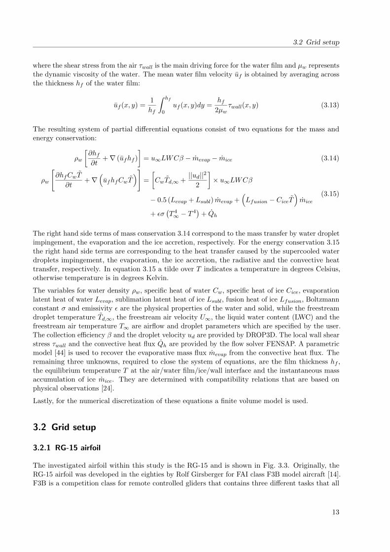
The resulting system of partial differential equations consist of two equations for the mass andenergy conservation:

ρw

[∂hf∂t

+∇ (ufhf )

]= u∞LWCβ − mevap − mice (3.14)

ρw

[∂hfCwT

∂t+∇

(ufhfCwT

)]=

[CwTd,∞ +

||ud||22

]× u∞LWCβ

− 0.5 (Levap + Lsubl) mevap +(Lfusion − CiceT

)mice

+ εσ(T 4∞ − T 4

)+ Qh

(3.15)

The right hand side terms of mass conservation 3.14 correspond to the mass transfer by water dropletimpingement, the evaporation and the ice accretion, respectively. For the energy conservation 3.15the right hand side terms are corresponding to the heat transfer caused by the supercooled waterdroplets impingement, the evaporation, the ice accretion, the radiative and the convective heattransfer, respectively. In equation 3.15 a tilde over T indicates a temperature in degrees Celsius,otherwise temperature is in degrees Kelvin.

The variables for water density ρw, specific heat of water Cw, specific heat of ice Cice, evaporationlatent heat of water Levap, sublimation latent heat of ice Lsubl, fusion heat of ice Lfusion, Boltzmannconstant σ and emissivity ε are the physical properties of the water and solid, while the freestreamdroplet temperature Td,∞, the freestream air velocity U∞, the liquid water content (LWC) and thefreestream air temperature T∞ are airflow and droplet parameters which are specified by the user.The collection efficiency β and the droplet velocity ud are provided by DROP3D. The local wall shearstress τwall and the convective heat flux Qh are provided by the flow solver FENSAP. A parametricmodel [44] is used to recover the evaporative mass flux mevap from the convective heat flux. Theremaining three unknowns, required to close the system of equations, are the film thickness hf ,the equilibrium temperature T at the air/water film/ice/wall interface and the instantaneous massaccumulation of ice mice. They are determined with compatibility relations that are based onphysical observations [24].

Lastly, for the numerical discretization of these equations a finite volume model is used.

3.2 Grid setup

3.2.1 RG-15 airfoil

The investigated airfoil within this study is the RG-15 and is shown in Fig. 3.3. Originally, theRG-15 airfoil was developed in the eighties by Rolf Girsberger for FAI class F3B model aircraft [14].F3B is a competition class for remote controlled gliders that contains three different tasks that all

13

3 Methods

0 0.1 0.2 0.3 0.4 0.5 0.6 0.7 0.8 0.9 1

0.0

0.1

Dimensionless x-coordinate x/c

Dim

ension

less

y-coordinate

y/c

Figure 3.3: 2D cross-section of the RG-15 airfoil.

start with a winch launch: thermal duration, distance flight and speed flight. Because all tasks haveto be flown with the same model, this competition class poses completely contradictory requirementson the model. The airfoil has to be optimized for flying with maximum lift during launching, withminimal sink rate in thermal duration task, with the best gliding ratio in the distance task andwith minimal drag in the speed task. The RG-15 performs well within all these tasks and wastherefore considered the benchmark for F3B airfoils for a long time. For this reason the RG-15 isalso well suited for the tasks of UAVs, for example, the PX-31 from Maritime Robotics, a fixed-wingunmanned aircraft with 3.2 m wingspan [32] used at the NTNU. With the RG-15 as part of thePX-31 system, all simulations of this study are setup with respect to the flight parameters of thePX-31, such as the flight speed and chord length.

3.2.2 Generation of the numerical grids

For the discretization of all airfoils in this study the commercial meshing software Pointwise (version18.2) has been used. Two different types of grids (subsequently named ice accretion and performancegrid) were created for the simulation of ice accretion and the simulation of aerodynamic performance.The different features of both grid types are summarized in Tab. 3.2 and shown in Fig. 3.4.

Both grids are set up as hybrid O-grid with a structured resolution of the boundary layer and anunstructured resolution of the far-field. The structured grid is better suited for the resolution of thevelocity profile near the airfoil’s surface, whereas the unstructured grid in the far-field ensures arestricted maximum element edge length and low skewness of the cells in the far-field. The trailingedge of the airfoil is set up blunt with a height of 1 mm to represent the airfoil geometry morerealistically. The initial cell height of both grids is set to ∆s = 1 · 10−6 m with a growth rate of 1.1for the structured layers, to get a dimensionless wall-distance for the first grid point of y+ ≤ 1. Thisensures an adequate resolution of the boundary layer and the viscous sublayer (which is defined to0 ≤ y+ ≤ 5 in [34]). This is necessary to capture the friction coefficient (for the simulation of iceaccretion) and the drag coefficient (for the performance simulation) correctly [34].

To get reliable results for the lift and drag coefficients, the performance grid is set up with a largerfar-field diameter (as listed in Tab. 3.2) and a higher resolution of the trailing edge. Additionally,for the creation of the performance grid, a so called ”T-Rex” technique provided by Pointwise isused for the generation of both the structured and unstructured grid. When the cell dimensions

14

3.2 Grid setup

(a) Variable number of structured layers - performance grid

(b) Constant number of structured layers - ice accretion grid

(c) Extrusion by one cell - performance grid (d) Discretization of the spanwise direction with triangu-lar elements - ice accretion grid

Figure 3.4: RG-15 grid setup for the (a), (c) performance grid and the (b), (d) ice accretion grid.

15

3 Methods

Feature Ice accretion grid Performance grid

Grid dimension 3D 2D

Chord length 0.45 m 0.45 m

Far-field diameter 9 m (20 c) 30 m (66.7 c)

Boundary layer (BL) resolution Constant number of struc-tured layers - 50 layers

Variable number of structuredlayers - ensures ideal isotropiccell height at the boundaryfrom structured to unstruc-tured grid

Initial cell height ∆s 1 · 10−6 1 · 10−6

Growth rate - structured layers 1.1 1.1

Spanwise discretization Triangular elements - fine res-olution of the leading edge tocapture the ice accretion

None - extrusion by one cell

Trailing edge setup Blunt - 1 mm height Blunt - 1 mm height

Number of cells ≈ 5 400 000 ≈ 80 000

Reference wing area 0.02025 m2 0.45 m2

Table 3.2: RG-15 grid feature comparison of the ice accretion and performance grid.

of the hexahedral cells used for the structured grid reach the ideal isotropic cell height, the gridwill be continued unstructured with prism elements. Using this method avoids large differences inthe element length of the last hexahedral and first prism layer and results in a variable number ofstructured layers around the airfoil, as shown in Fig. 3.4a. Lastly, an extrusion of the grid by onecell in spanwise direction is required (see Fig. 3.4c), since FENSAP-ICE determines the lift anddrag coefficients based on the resultant forces for lift L and drag D according to the equations 3.16and 3.17 and therefore needs a reference wing area A.

cl =2L

ρu2∞A(3.16)

cd =2D

ρu2∞A(3.17)

The ice accretion grid requires a three-dimensional grid with a high resolution around the leadingedge to gain a sufficient resolution of the ice shape. Therefore the surface of the airfoil in spanwisedirection is discretized with triangular elements, as shown in Fig. 3.4d. This approach changes theelement type for the structured grid from hexahedrons to triangular prisms and for the unstructureddiscretization of the far-field from prims to tetrahedrons. The additional fine resolution of theairfoil in the third dimension significantly increases the number of cells for the overall grid. For thisreason and since the focus for the ice accretion grid is on a fine resolution of the leading edge, ratherthan a precise determination of aerodynamic coefficients, a smaller far-field, a constant number ofstructured layers (see Fig. 3.4b) and a smaller spanwise extrusion is initialized, to keep the numberof cells within reasonable range.

Using this grid, all ice accretion simulations result in a three dimensional ice shape with a width of4.5 cm, as shown in Fig. 3.5. Since the performance of two dimensional airfoils is being investigated,

16

3.3 Grid dependency study

Figure 3.5: 3D ice shape result of an ice accretion simulation on an RG-15 airfoil and the positionof the cross-section that is being used for the 2D evaluation.

only one cross-section of the iced airfoil will be presented as result of the ice accretion. Morespecifically, the cross-section in the center of the 3D airfoil, in spanwise direction as shown inFig. 3.5, will be used in all cases. This procedure enables a fast visualization of two dimensionalice accretion results. However, it should be mentioned that a single cross-section only represents aspecific ice shape at this position but neglects variations of the ice shape over the three dimensionalwing.

3.3 Grid dependency study

A grid dependency study is performed in order to determine the dependency between the simulationresults and the resolution of the mesh to ensure the use of a sufficient grid resolution that doesnot falsify the results. Commonly, the truncation error of the simulation and the resolution of thegrid are inversely proportional, whereas simulation time and resolution are proportional. With thedependency study, a compromise between simulation time and accuracy of the results is found.This is done by calculating lift and drag coefficients and an estimation of the exact result based onextrapolation, and comparing the error and the simulation times. For the estimation of the exactresult φ a Richard extrapolation can be performed. It is based on the simulation results for threedifferent grids φh, φkch and φk2ch, the constant ratio kc of the discretization parameter between thegrids and the rate of convergence r, see [34]:

φ = φh +φh − φkchkrc − 1

(3.18)

The calculation is based on the converged simulations of three different grids to which εit � εhapplies for the iteration error, and the hypothesis that the constant of proportionality for all threesimulations is constant and independent from the discretization parameter h. In case of a 2D airflowsimulation around an airfoil, the latter parameter will be defined as:

17

3 Methods

h =c

n(3.19)

with airfoil chord length c and n the number of points discretizing the upper and lower surface ofthe airfoil respectively. The parameter kc is determined with respect to the following coherence:

h3 = k2ch1

h2 = kch1

h1 = kc

(3.20)

The rate of convergence is estimated as follows:

r =

log

(φkch−φk2chφh−φkch

)log(kc)

(3.21)

It is important to mention that the estimation for the rate of convergence is only valid if thesimulation results are converging monotonously. With the use of equations 3.19 to 3.21 in 3.18 theexact result φ can be calculated.

The results for the grid dependency studies are presented in Ch. 4, together with the general setupand the validation of the different simulation models that are used.

3.4 Meteorological icing conditions

For the certification of large aircraft, 14 CFR Part 25 Appendix C of the Federal AviationAdministration (FAA) regulations [12] contains two different envelopes that define icing conditions:

Continuous maximum: Stratiform clouds with a horizontal extent of 17.4 nm (32.2 km) and anapplicable pressure altitude range of sea level to 22 000 ft (6 700 m).

Intermittend maximum: Cumuliform clouds with a horizontal extend of 2.6 nm (4.8 km) and anapplicable pressure altitude range of 4 000-22 000 ft (1 200-6 700 m).

With the applicable pressure altitude range down to sea level, the continuous maximum icingconditions include the low flight altitudes of small-sized UAVs. Furthermore, the larger horizontalcloud extend results in longer icing durations. For these reasons, all icing cases investigated inthis work are chosen within the envelope of the maximum continuous icing conditions of the FAArequirements. Figure 3.6 gives an overview over the icing envelope where the 16 different conditionsthat are going to be investigated in this work are marked red. They are defined by the droplet’smedian volume diameter (MVD), the icing temperature and the liquid water content (LWC) andcover a temperature range of -30 ◦C to -2 ◦C, a median volume diameter range of 15 µm to 40 µmand the corresponding liquid water content of 0.038 g/m3 to 0.760 g/m3. In Tab. 3.3 all parametersof the 16 conditions including the corresponding LWC are listed.

18

3.4 Meteorological icing conditions

15 20 25 30 35 40

0

0.2

0.4

0.6

0.8

Air

temp.

0 ◦C

−10 ◦

C

−20 ◦C

−30 ◦C

Median volume diameter µm

Liquid

watercontentg/

m3

Figure 3.6: Weather conditions covered withinthis study in comparison to theCFR 14 Part 25 App. C icing en-velope for maximum continuous ic-ing.

MVD [µm]Ticing [◦C]

-2 -5 -15 -30

15 0.760 0.700 0.450 0.200

20 0.595 0.531 0.319 0.141

30 0.347 0.299 0.165 0.070

40 0.140 0.125 0.078 0.038

Table 3.3: LWC in g/m3 as function of MVDand temperature.

19

4 Simulation models and validation

Prior to the simulation of ice accretion and performance the simulation models have to be set upand validated for all the 16 previously described icing cases. Therefore, this chapter includes thegrid dependency results for the performance grid, a time-step study for the ice accretion grid andthe validation of both simulation models.

4.1 Clean airfoil performance model

The first step towards a simulation model for determining the aerodynamic performance is a griddependency study and a validation of the clean airfoil to verify the simulation results an un-icedairfoil. The validation of the clean airfoil performance is based on experimental data of two windtunnel tests with the RG-15 airfoil at a Reynolds numbers of Re = 200 000, published in [35] and [33].The validation data are somehow problematic, since the Reynolds number does not match the onepresent for the simulations of this work. All performance simulations in this work are performed ata Reynolds number of Re = 800 000. That means, the relation of inertia to viscous forces are notcorrectly represented by the validation. Since this relation is decisive for correct modeling of theboundary layer, it ultimately affects the results for the aerodynamic forces. However, due to thelack of experimental data at correct Reynolds numbers this had to be accepted.

4.1.1 Grid dependency study

For the grid dependency study on the performance grid, three different resolutions with n = 80(grid A), 160 (grid B) and 320 (grid C) have been created. All simulations are performed at anangle of attack of +4◦, which represents a typical AoA for straight and level flight. Except theresolution of the grid, all other setup parameters, summarized in Tab. 4.1, were kept constant inorder to evaluate only the influence of the grid resolution. The simulation results for lift an drag ofall three grids are presented in Fig. 4.1.

Parameter Value

Chord length c 0.45 m

Free stream velocity u∞ 6.5 m/s

Static pressure p 101325 Pa

Air temperature T 288.15 K

Reynolds number Re 200 000

Angle of Attack α 4◦

Table 4.1: Simulation parameter for the grid dependency study.

21

4 Simulation models and validation

0.000

0.001

0.002

0.003

0.004

0.005

0.006

0.665

0.666

0.667

0.668

extrapolated exact result

CB

A

Discretization parameter h

Lif

tco

effici

entc l

(a)

0.000

0.001

0.002

0.003

0.004

0.005

0.006

0.01110

0.01115

0.01120

0.01125

C

B

A

Discretization parameter h

Dra

gco

effici

entc d

(b)

Figure 4.1: Simulation results of grids A to C and the extrapolated exact result for the griddependency study for the clean RG-15 airfoil grid.

As the results show, only the values for the lift coefficient are converging monotonously. Therefore,a Richardson extrapolation according to the equations 3.18 to 3.21 has only been performed onthe results for the lift. For the drag results no exact result has been estimated. Regarding the liftcoefficient, the grid with the least points at n = 80, grid A, already shows a good result with adeviation of 0.5 % to the accurate result. The comparison of grid A and grid B for the drag revealsa maximum deviation of 0.1 % within all three different grids. With only negligible differences of allresults, all grids are considered suitable in terms of accuracy. The comparison of simulation timeprovided additional information about the suitability of the grid. Although grid B consists of twicethe amount of points compared to grid A, the fastest simulation time of all grids to reach similarconvergence level was found with grid B with 21 min, whereas the simulation time for was 26 minand 23 min for grid A and C, respectively. With respect to the simulation time and only negligibledifferences between the lift and drag results, grid B resolution will be used for the simulation ofclean airfoil performance.

4.1.2 Performance validation

As mentioned in Sec. 3.1.2, two simulations were performed using the k-ω-SST and the SpalartAllmaras (SA) turbulence model. For the k-ω-SST model transition is predicted by a one-equationlocal correlation-based intermittency model, whereas the SA turbulence model is set up withfixed transition locations, previously determined with XFOIL. Further simulation parameters forthe validation, except the angle of attack, are setup similarly as for the grid dependency study,refer to Tab. 4.1. The pressure and temperature are set in accordance with the ICAO standardatmosphere [25] at an altitude of 0 m and the free stream velocity is set to 6.5 m/s resulting in aReynolds number of approximately Re = 200 000 to match the Reynolds number of the experimentaldata. The simulation results for the lift and drag coefficient in comparison to the experimental dataare presented in Fig. 4.2.

22

4.1 Clean airfoil performance model

−8 −6 −4 −2 0 2 4 6 8 10 12−0.6

−0.4

−0.2

0

0.2

0.4

0.6

0.8

1

1.2

Angle of attack α

Lif

tco

effici

entc l

Illinois 1995 (Selig)

Stuttgart (Rozehnal)FENSAP-ICE k-w-SSTintermittency transitionFENSAP-ICE SAfixed transition (XFOIL)

(a)

−8 −6 −4 −2 0 2 4 6 8 10 12

0.01

0.02

0.03

0.04

0.05

0.06

0.07

Angle of attack α

Dra

gco

effici

entc d

Illinois 1995 (Selig)

Stuttgart (Rozehnal)FENSAP-ICE k-w-SSTintermittency transitionFENSAP-ICE SAfixed transition (XFOIL)

(b)

Figure 4.2: (a) Lift and (b) drag results for the clean RG-15 airfoil performance compared to theexperimental data, Re = 200 000.

23

4 Simulation models and validation

In general both simulation results show a good agreement with the experimental results. For anAoA between −3◦ to −1◦ both simulations show a small deviation of predicted lift coefficients tothe experimental data. A possible explanation could be that the simulations both predict slightlyearlier transition from laminar to turbulent boundary layer.

The stall is captured within reasonable precision to the experimental results with both turbulencemodels. The simulation model using the k-ω-SST model predicts a lower maximum lift coefficientand lower maximum lift angle, compared to the SA model. The drag prediction of both simulationsshows good agreement to the experimental results for the entire AoA range. For AoAs >7◦, withthe onset of the stall, the comparison of the turbulence models shows that the k-ω-SST predictshigher drag as the SA model. In total, both simulation models predict lift and drag coefficientswithin close range to the experimental results.

4.2 Iced airfoil performance model

Following the validation of the clean airfoil, a grid dependency study and validation are performedon an iced airfoil to verify the simulation results for the iced airfoil performance. Since no suitableliterature data of an iced RG-15 airfoil was found, wind tunnel test results of an iced NREL S826airfoil at a Reynolds number of Re = 400 000, published in [9], were used instead. The data for theiced NREL S826 are gathered by 3D-printing the simulated ice geometry and attaching it to theclean airfoil for the wind tunnel tests. As for the clean airfoil validation no experimental data wasavailable that matched the Reynolds numbers of the simulations in this work.

4.2.1 Grid dependency study

In this case, for the grid dependency study, the grid for the NREL S826 airfoil was created withfour different resolutions: n = 80 (grid A), 160 (grid B), 226 (grid C) and 320 (grid D). However,since an iced airfoil has a much more complex shape, the performance grid for an iced airfoil had tobe adapted as shown in Fig. 4.3. The discretization parameter h now only describes the surface ofthe airfoil without the iced leading edge. For the resolution of the leading edge, a higher number ofpoints with constant spacing is set up to capture the ice shape sufficiently. For the grid dependencystudy the number of points discretizing the leading edge are scaled with the same factor as theparameter n and range from 150 to 600 points. An additional grid with an intermediate number of

Figure 4.3: Numerical grid for the iced S826 airfoil performance simulation.

24

4.2 Iced airfoil performance model

0.000

0.001

0.002

0.003

0.004

0.005

0.006

0.798

0.800

0.802

0.804

0.806 D

C

BA

Discretization parameter h

Lif

tco

effici

entc l

(a)

0.000

0.001

0.002

0.003

0.004

0.005

0.006

0.0652

0.0654

0.0656

0.0658

DC

B

A

Discretization parameter hD

rag

coeffi

cien

tc d

(b)

Figure 4.4: Simulation results of grids A to D for the grid dependency study for the iced S826airfoil grid.

points of 226 (grid C) was set up, should the calculation time for grid B prove to be excessive. Thiswas not the case so that grid C was not used in the end. The simulation parameters are set upidentically to the first grid dependency study (ref. to Tab. 4.1), except for the free stream velocity.The free stream velocity was changed to 13 m/s to match the Reynolds number Re = 400 000 of theexperimental data.

The results based on the four different grids are presented in Fig. 4.4. Since the results for bothlift and drag are not converging monotonously, a Richardson Extrapolation is not valid in thiscase. That means that the values for lift and drag coefficients can not be checked against ananalytically estimated exact result. The comparison of grid A and D however, reveals a differenceof approximately 1 % for both lift and drag coefficient. The small deviation, despite a four timeshigher resolution of grid D, indicates a low truncation error and a suitable result already for grid A.The simulation times for grid A, B, C and D were 9.5 min, 9 min, 11 min and 14 min, respectively.Therefore, the grid resolution with the least number of iterations and shortest simulation time (gridB) will be used for the validation.

4.2.2 Performance validation

For the validation of iced airfoil performance, the SA turbulence model and a fully turbulentboundary layer are set up for the simulation. Further parameters are similar to those for the griddependency study to match the Reynolds number of the experimental data.

Figure 4.5 presents the simulation results in comparison to the wind tunnel data. For the AoAsbetween −8◦ and 0◦, the simulation shows generally good agreement with the experimental data.For higher angles of attack the simulation shows a smaller lift gradient. Regarding the stall, thesimulation predicts an earlier stall at a lower AoA and a lower maximum lift coefficient. In terms ofdrag, the simulation captures a similar trend of drag over AoA but under-predicts the drag at all

25

4 Simulation models and validation

−6 −4 −2 0 2 4 6 8 10

0

0.2

0.4

0.6

0.8

1

Angle of attack α

Lif

tco

effici

entc l

Experimental (NTNU)FENSAP-ICE SA

(a)

−6 −4 −2 0 2 4 6 8 10

0.05

0.1

0.15

0.2

0.25

Angle of attack α

Dra

gco

effici

entc d

Experimental (NTNU)FENSAP-ICE SA

(b)

Figure 4.5: (a) Lift and (b) drag results for the iced S826 airfoil performance compared to theexperimental data, Re = 400 000.

26

4.3 Ice accretion model

Figure 4.6: Large flow separation at the leading edge of the iced S826 NREL airfoil, AoA 5◦ andRe = 400 000.

points. The reason for the diverging results is suspected to be in the use of the turbulence model(Spalart-Allmaras) in combination with a high level of turbulence, caused by the horns. The surfaceroughness and the horn shape result in a high level of turbulence and a large flow separation at theleading edge already at very low AoAs, as shown in Fig. 4.6 for an AoA of 5◦. In the literature it isgenerally admitted that one- and two-equation turbulence models, like the SA model for example,have difficulties to accurately predict the flow field in a separated region [3]. For the degree ofturbulence and separated flow at the leading edge, like in this case, different numerical methodslike LES and DNS or higher order turbulence models like nonlinear eddy viscosity models andReynolds stress models might be more suitable. An error of the simulation results due to the steadyflow simulation is conceivable but the simulation did not show any indications that steady flowsimulation might lead to false results. The numerical residual reaches the convergence thresholdof 1−10 at all angles of attack before reaching the maximum number of time steps and does notlevel off at higher values with oscillation of the residual. However, no conclusive explanation for thedeviation of simulation and experimental results has been found.

Further, it must be mentioned that the icing conditions for the experimental data in this case havebeen specifically chosen to create severe icing with a horn shaped structure. To achive that, severalicing parameters were modified. In particular, the icing time was set to 40 min, twice of what isused in this work. For a detailed listing of the parameters, see [23]. Therefore, a much smallerextend of ice, less turbulence intensity and less severe flow separation at the leading edge, especiallyfor higher angles of attack, is expected for the icing cases in this work.

Given the general agreement of the simulation results for all AoAs, the results of the simulation modelare considered adequate for evaluating iced airfoil performance. Discrepancies can be explained bythe high turbulence intensity due to the large horn extrusions. Due to the less severe ice shapesexpected in this work without the horn features, this is deemed acceptable. Further, at least for thelift coefficient, the simulation predicts more conservative values.

4.3 Ice accretion model

A different approach than the grid dependency studies for the performance model was chosen forthe simulation model of the ice accretion. For this simulation model a grid dependency study isnot representative since the focus for this model is on capturing the ice shape adequately, ratherthan predicting precise lift and drag coefficients. For this reason a time-step study instead of a grid

27

4 Simulation models and validation

Parameter Rime ice case Glaze ice case

Chord length c 0.45 m 0.45 m

Free stream velocity u∞ 25 m/s 25 m/s

Static pressure p / flight altitude 95 500 Pa / 500 m 95 500 Pa / 500 m

Air temperature T −15 ◦C −2 ◦C

Median volume diameter MVD 20 µm 20 µm

Droplet size distribution Monodisperse Monodisperse

Reynolds number Re 880 000 810 000

Angle of Attack α 0◦ 0◦

Icing time ticing 1 290 s / 21.5 min 1 290 s / 21.5 min

Initial roughness height ks 0.5 mm 0.5 mm

number of steps / step length (1.step length / 10 (129 s) 5 (30 s/315 s)

other step length) 15 (30 s/90 s) 10 (30 s/140 s)

22 (30 s/60 s) 22 (30 s/60 s)

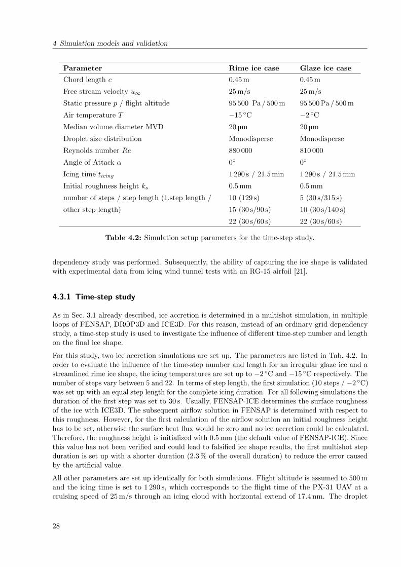
Table 4.2: Simulation setup parameters for the time-step study.

dependency study was performed. Subsequently, the ability of capturing the ice shape is validatedwith experimental data from icing wind tunnel tests with an RG-15 airfoil [21].

4.3.1 Time-step study

As in Sec. 3.1 already described, ice accretion is determined in a multishot simulation, in multipleloops of FENSAP, DROP3D and ICE3D. For this reason, instead of an ordinary grid dependencystudy, a time-step study is used to investigate the influence of different time-step number and lengthon the final ice shape.

For this study, two ice accretion simulations are set up. The parameters are listed in Tab. 4.2. Inorder to evaluate the influence of the time-step number and length for an irregular glaze ice and astreamlined rime ice shape, the icing temperatures are set up to −2 ◦C and −15 ◦C respectively. Thenumber of steps vary between 5 and 22. In terms of step length, the first simulation (10 steps / −2 ◦C)was set up with an equal step length for the complete icing duration. For all following simulations theduration of the first step was set to 30 s. Usually, FENSAP-ICE determines the surface roughnessof the ice with ICE3D. The subsequent airflow solution in FENSAP is determined with respect tothis roughness. However, for the first calculation of the airflow solution an initial roughness heighthas to be set, otherwise the surface heat flux would be zero and no ice accretion could be calculated.Therefore, the roughness height is initialized with 0.5 mm (the default value of FENSAP-ICE). Sincethis value has not been verified and could lead to falsified ice shape results, the first multishot stepduration is set up with a shorter duration (2.3 % of the overall duration) to reduce the error causedby the artificial value.

All other parameters are set up identically for both simulations. Flight altitude is assumed to 500 mand the icing time is set to 1 290 s, which corresponds to the flight time of the PX-31 UAV at acruising speed of 25 m/s through an icing cloud with horizontal extend of 17.4 nm. The droplet

28

4.3 Ice accretion model

−0.02 0.00 0.02 0.04 0.06 0.08

−0.02

0.00

0.02

0.04

Dimensionless x-coordinate x/c

Dim

ension

less

y-coordinate

y/c

10 steps (129 s)

15 steps (30 s/90 s)

22 steps (30 s/60 s)Clean airfoil

(a)

−0.02 0.00 0.02 0.04 0.06 0.08

−0.02

0.00

0.02

0.04

Dimensionless x-coordinate x/c

Dim

ension

less

y-coordinate

y/c

5 steps (30 s/315 s)

10 steps (30 s/140 s)

22 steps (30 s/60 s)Clean airfoil

(b)

Figure 4.7: Time-step study results for a (a) rime ice and (b) glaze ice case on the RG-15 airfoil.

size distribution for all ice accretion simulations in this work is set to monodisperse for reasons ofcomparability of the ice shape results. This setup eliminates the influence of differently distributeddroplet sizes on the ice accretion process. The results of the time-step study are presented in Fig. 4.7.

The rime ice case generally shows congruent geometries and icing limits for all three simulations.The comparison of the 10 step to the 22 step simulation reveals that an increased number ofsimulation steps results in a slightly smoother surface, which can be best seen when comparing thebumps on the upper surface. The calculation times using 40 Intel Xeon E5-2670 processors witha total of 320 cores were approximately 8 h (10 steps), 10 h (15 steps) and 18 h (22 steps). Theice masses of all three simulations are similar, with a variation of less than 1 %. Considering thesmall changes of the ice shapes, the 15 step simulation offers the best results with only 2 h longercalculation time compared to 10 steps but 8 h less than 22 steps.

For the glaze ice case a different behavior can be observed. In this case an increasing number ofsteps results in a more irregular shape. In general, the shapes of 10 and 22 steps are relativelysimilar. The 5 step simulation however shows a higher ice thickness further downstream on theairfoil but an overall smoother surface. The reason for this behavior is suspected to be in thecombination of a temperature close to freezing and a long step duration. At temperatures close tofreezing, more liquid water remains on the surface, whereas at lower temperatures all impingingwater freezes instantly. The long duration allows the water to run further back on the surface beforefreezing. Therefore, the results with 10 and 22 steps are expected to represent a more realisticice shape for these icing conditions. Regarding the ice mass, increasing the number of steps from10 to 22 results in a change of less than 5 %. Using the same number of cores as for the rime icecase, the calculation times for 10 steps was 8 h and for 22 steps 20 h.

Keeping the wide range of meteorological conditions that are going to be investigated in this studyin mind, no accurate prediction on the ice shapes for those conditions can be made. Therefore aconsistent number and duration of steps for all ice accretion simulations is desired. For the rime icecase a 15 step simulation was rated the best compromise between number of steps and calculationtime. For the glaze ice case 10 and 22 step showed similar results in terms of final ice shape. No 15

29

4 Simulation models and validation

Parameter Rime Glaze

Free stream velocity u∞ 25 m/s 25 m/s

Chord length c 0.45 m 0.45 m

Icing time ticing 1 200 s 1 200 s

Angle of attack α 0◦ 0◦

Air temperature T −15 ◦C −2 ◦C

Median volume diameter MVD 20 µm 30 µm

Liquid water content LWC 0.51 g/m3 0.51 g/m3

Table 4.3: Simulation setup parameters for the ice accretion validation.

step simulation was done for the glaze ice case. A comparison of calculation times for rime andglaze ice cases at 22 steps indicates a 2 h longer calculation time for glaze ice.

With respect to the final ice shapes and the calculation times, a 15 step setup with 30 s duration forthe first and 90 s duration for the following steps is selected for all ice accretion simulations. Thecalculation time is expected to be approximately 10 h to 13 h depending on the icing condition.

4.3.2 Ice accretion validation

With completion of the time-step study, the simulation model for ice accretion is prepared forvalidation. Therefore, two different icing cases, again for a rime and a glaze ice case, were chosenfrom the experimental results within [21]. The setup parameters for both experiments are listedin Tab. 4.3 and are also used for the simulation. Again, as mentioned in Sec. 3.1.2, due to thepresence of ice, the boundary layer is set up fully turbulent and the SA model is used for turbulencemodeling.

0.00 0.05 0.10

−0.02

0.00

0.02

0.04

Dimensionless x-coordinate x/c

Dim

ensionless

y-coordinatey/c

ExperimentalFENSAP-ICEClean airfoil

(a)

0.00 0.05 0.10 0.15−0.04

−0.02

0.00

0.02

0.04

0.06

Dimensionless x-coordinate x/c

Dim

ension

less

y-coordinate

y/c

ExperimentalFENSAP-ICEClean airfoil

(b)

Figure 4.8: Simulation results for the ice accretion at a (a) rime ice and (b) glaze ice case on theRG-15 airfoil, compared to wind tunnel results.

30

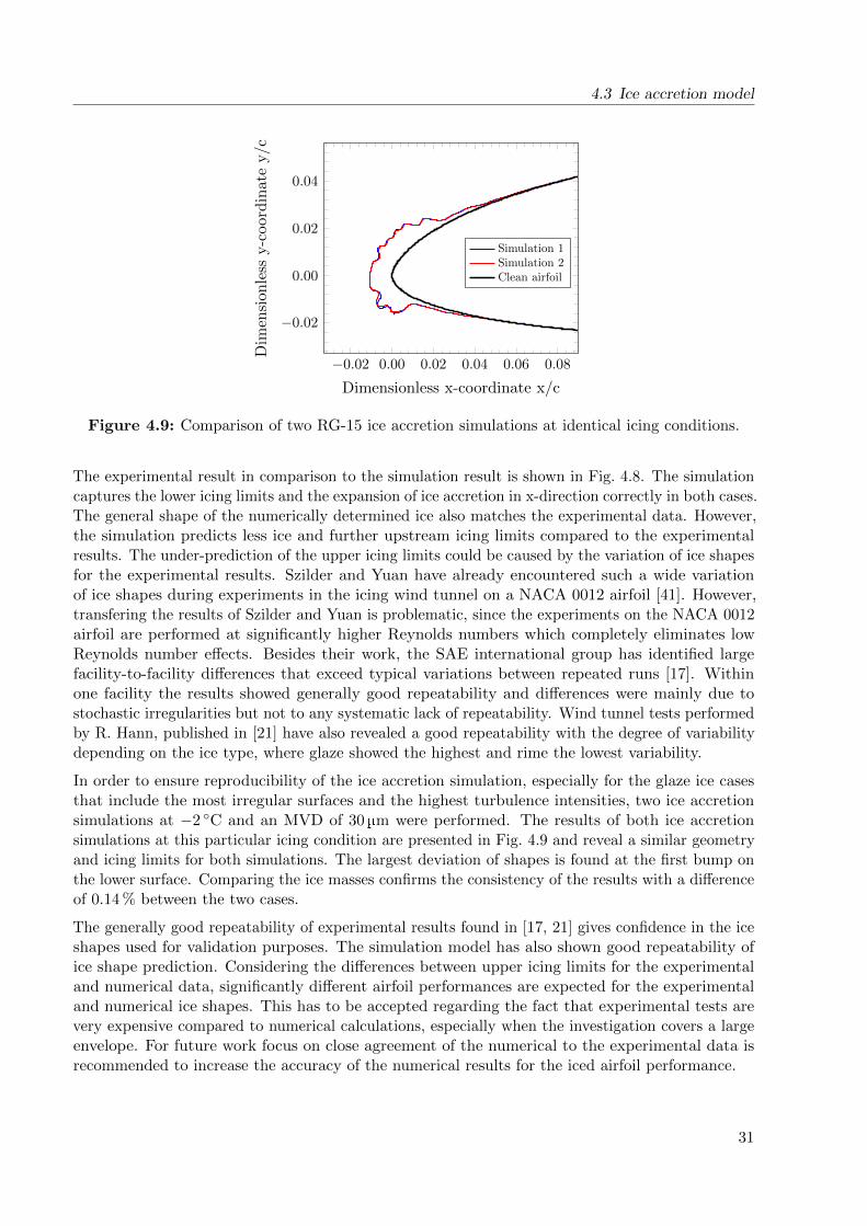
4.3 Ice accretion model

−0.02 0.00 0.02 0.04 0.06 0.08

−0.02

0.00

0.02

0.04

Dimensionless x-coordinate x/c

Dim

ension

less

y-coordinate

y/c

Simulation 1Simulation 2Clean airfoil

Figure 4.9: Comparison of two RG-15 ice accretion simulations at identical icing conditions.

The experimental result in comparison to the simulation result is shown in Fig. 4.8. The simulationcaptures the lower icing limits and the expansion of ice accretion in x-direction correctly in both cases.The general shape of the numerically determined ice also matches the experimental data. However,the simulation predicts less ice and further upstream icing limits compared to the experimentalresults. The under-prediction of the upper icing limits could be caused by the variation of ice shapesfor the experimental results. Szilder and Yuan have already encountered such a wide variationof ice shapes during experiments in the icing wind tunnel on a NACA 0012 airfoil [41]. However,transfering the results of Szilder and Yuan is problematic, since the experiments on the NACA 0012airfoil are performed at significantly higher Reynolds numbers which completely eliminates lowReynolds number effects. Besides their work, the SAE international group has identified largefacility-to-facility differences that exceed typical variations between repeated runs [17]. Withinone facility the results showed generally good repeatability and differences were mainly due tostochastic irregularities but not to any systematic lack of repeatability. Wind tunnel tests performedby R. Hann, published in [21] have also revealed a good repeatability with the degree of variabilitydepending on the ice type, where glaze showed the highest and rime the lowest variability.

In order to ensure reproducibility of the ice accretion simulation, especially for the glaze ice casesthat include the most irregular surfaces and the highest turbulence intensities, two ice accretionsimulations at −2 ◦C and an MVD of 30 µm were performed. The results of both ice accretionsimulations at this particular icing condition are presented in Fig. 4.9 and reveal a similar geometryand icing limits for both simulations. The largest deviation of shapes is found at the first bump onthe lower surface. Comparing the ice masses confirms the consistency of the results with a differenceof 0.14 % between the two cases.

The generally good repeatability of experimental results found in [17, 21] gives confidence in the iceshapes used for validation purposes. The simulation model has also shown good repeatability ofice shape prediction. Considering the differences between upper icing limits for the experimentaland numerical data, significantly different airfoil performances are expected for the experimentaland numerical ice shapes. This has to be accepted regarding the fact that experimental tests arevery expensive compared to numerical calculations, especially when the investigation covers a largeenvelope. For future work focus on close agreement of the numerical to the experimental data isrecommended to increase the accuracy of the numerical results for the iced airfoil performance.

31

5 Ice accretion results and performancedegradation

With completed validation of both simulation models, they can be used for determining the iceaccretion and the aerodynamic performance for all different icing conditions that were previouslydefined in Sec. 3.4. In this chapter the simulation results are presented. Further, the influence of thedifferent meteorological conditions and the relevance of the results with respect to the developmentof an IPS system for UAVs are discussed and uncertainties of the work are pointed out.

5.1 Ice accretion

In total, 16 meteorological icing conditions, defined by different droplet sizes, temperatures andliquid water contents are being investigated. The detailed values for all icing conditions are listed inTab. 3.3 in Sec. 3.4. All additional setup parameters for the ice accretion simulation are summarizedin Tab. 5.1 and 5.2. The final ice shapes are presented in Fig. 5.1.

For reasons of readability, the MVD will be mentioned without unit at some points. The resultsshow that both liquid water content and droplet diameter have significant influence on the ice shape.As previously shown in Fig. 3.6, droplets with small MVDs around 15 µm can contain a higherrange of liquid water content compared to large MVDs. Therefore, the results at a temperatureof −2 ◦C and droplet diameters 15, 20 and 30 show a distinct glaze ice shape with an irregularsurface. The mass balance supports the assumption of a glaze ice structure, as not all impingingwater freezes instantly but some liquid water remains on the surface. At a droplet diameter of 40 µm,the maximum liquid water content has decreased to a point where all results show a streamlineshaped ice geometry, independently from the prevailing temperatures. All results at the diameterof 40 µm are close to the un-iced airfoil geometry. The extend only differs slightly, depending on the

Parameter Value

Chord length c 0.45 m

Free stream velocity u∞ 25 m/s

Static pressure p 95 500 Pa

Reynolds number Re 800 000 - 1 000,000

Angle of Attack AoA 0◦

Icing time ticing 1 290 s

Droplet size distribution Monodisperse

Initial roughness height ks 0.5 mm

Table 5.1: Setup parameters for the simulation of ice accretion.

33

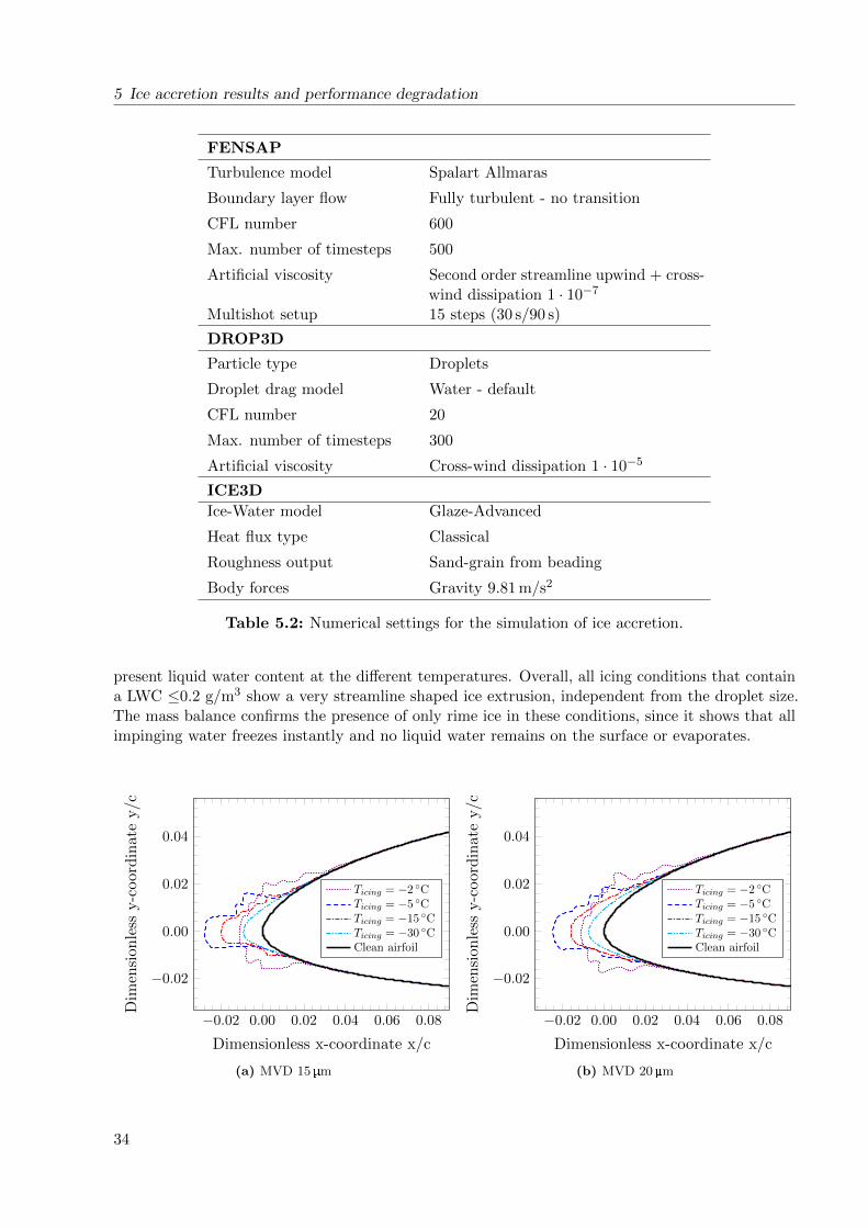
5 Ice accretion results and performance degradation

FENSAP

Turbulence model Spalart Allmaras

Boundary layer flow Fully turbulent - no transition

CFL number 600

Max. number of timesteps 500

Artificial viscosity Second order streamline upwind + cross-wind dissipation 1 · 10−7

Multishot setup 15 steps (30 s/90 s)

DROP3D

Particle type Droplets

Droplet drag model Water - default

CFL number 20

Max. number of timesteps 300

Artificial viscosity Cross-wind dissipation 1 · 10−5

ICE3D

Ice-Water model Glaze-Advanced

Heat flux type Classical

Roughness output Sand-grain from beading

Body forces Gravity 9.81 m/s2

Table 5.2: Numerical settings for the simulation of ice accretion.

present liquid water content at the different temperatures. Overall, all icing conditions that containa LWC ≤0.2 g/m3 show a very streamline shaped ice extrusion, independent from the droplet size.The mass balance confirms the presence of only rime ice in these conditions, since it shows that allimpinging water freezes instantly and no liquid water remains on the surface or evaporates.

−0.02 0.00 0.02 0.04 0.06 0.08

−0.02

0.00

0.02

0.04

Dimensionless x-coordinate x/c

Dim

ension

less

y-coordinatey/c

Ticing = −2 ◦CTicing = −5 ◦CTicing = −15 ◦CTicing = −30 ◦CClean airfoil

(a) MVD 15µm

−0.02 0.00 0.02 0.04 0.06 0.08

−0.02

0.00

0.02

0.04

Dimensionless x-coordinate x/c

Dim

ension

less

y-coordinatey/c

Ticing = −2 ◦CTicing = −5 ◦CTicing = −15 ◦CTicing = −30 ◦CClean airfoil

(b) MVD 20µm

34

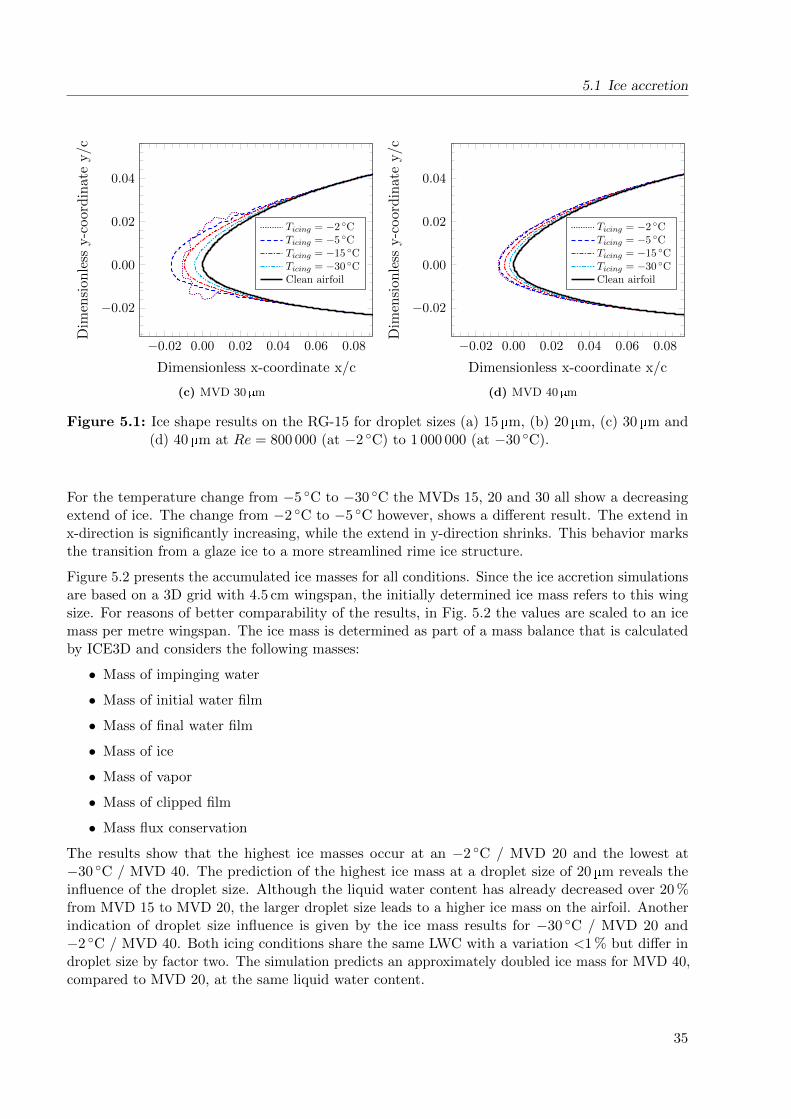
5.1 Ice accretion

−0.02 0.00 0.02 0.04 0.06 0.08

−0.02

0.00

0.02

0.04

Dimensionless x-coordinate x/c

Dim

ension

less

y-coordinate

y/c

Ticing = −2 ◦CTicing = −5 ◦CTicing = −15 ◦CTicing = −30 ◦CClean airfoil

(c) MVD 30µm

−0.02 0.00 0.02 0.04 0.06 0.08

−0.02

0.00

0.02

0.04

Dimensionless x-coordinate x/c

Dim

ension

less

y-coordinate

y/c

Ticing = −2 ◦CTicing = −5 ◦CTicing = −15 ◦CTicing = −30 ◦CClean airfoil

(d) MVD 40 µm

Figure 5.1: Ice shape results on the RG-15 for droplet sizes (a) 15 µm, (b) 20 µm, (c) 30 µm and(d) 40 µm at Re = 800 000 (at −2 ◦C) to 1 000 000 (at −30 ◦C).

For the temperature change from −5 ◦C to −30 ◦C the MVDs 15, 20 and 30 all show a decreasingextend of ice. The change from −2 ◦C to −5 ◦C however, shows a different result. The extend inx-direction is significantly increasing, while the extend in y-direction shrinks. This behavior marksthe transition from a glaze ice to a more streamlined rime ice structure.

Figure 5.2 presents the accumulated ice masses for all conditions. Since the ice accretion simulationsare based on a 3D grid with 4.5 cm wingspan, the initially determined ice mass refers to this wingsize. For reasons of better comparability of the results, in Fig. 5.2 the values are scaled to an icemass per metre wingspan. The ice mass is determined as part of a mass balance that is calculatedby ICE3D and considers the following masses:

• Mass of impinging water

• Mass of initial water film

• Mass of final water film

• Mass of ice

• Mass of vapor

• Mass of clipped film

• Mass flux conservation

The results show that the highest ice masses occur at an −2 ◦C / MVD 20 and the lowest at−30 ◦C / MVD 40. The prediction of the highest ice mass at a droplet size of 20 µm reveals theinfluence of the droplet size. Although the liquid water content has already decreased over 20 %from MVD 15 to MVD 20, the larger droplet size leads to a higher ice mass on the airfoil. Anotherindication of droplet size influence is given by the ice mass results for −30 ◦C / MVD 20 and−2 ◦C / MVD 40. Both icing conditions share the same LWC with a variation <1 % but differ indroplet size by factor two. The simulation predicts an approximately doubled ice mass for MVD 40,compared to MVD 20, at the same liquid water content.

35

5 Ice accretion results and performance degradation

−30 −25 −20 −15 −10 −5 0

0.5

1

1.5

2

2.5

Temperature ◦C

Icemasskg/

m

MVD 15 µmMVD 20 µmMVD 30 µmMVD 40 µm

Figure 5.2: Simulation results for the accumulated ice masses on the RG-15.

The results further show a complex influence of droplet MVD and liquid water content on the overallice mass. Increasing the droplet size from 15 to 20 results in a higher ice mass at all temperatures,although the liquid water content decreases consistently, whereas the increase from MVD 20 to 30and 40 results in lower ice masses. This arises the impression that the droplet size is the predominantfactor on the ice mass at high liquid water contents and generally smaller droplet sizes, whereas foroverall larger droplets and low LWCs, the decreasing LWC becomes the predominant factor.

Comparing MVD 15 and 30, the results of MVD 30 µm show higher ice masses for temperatures −2 ◦Cand −5 ◦C and lower ice masses for the temperatures −15 ◦C and −30 ◦C. This indicates that theshift from increasing droplet size to decreasing liquid water content being the dominating factor onthe ice mass occurs at different droplet sizes, depending on the temperature. Finally, within allconditions, the temperature change from −2 ◦C to −5 ◦C at an MVD of 30 µm shows a unique result.Only for this particular case, a decreasing temperature at the same droplet size, leads to a higher icemass. At first thought this result appears physically not correct, since the decreasing temperatureat the same droplet size contains less liquid water, according to the icing envelope. But as themass balances shows, there are more factors to consider. For all four droplet sizes the total massof impinging water is higher at −2 ◦C but the amount of remaining liquid water and the mass ofevaporating water is much higher at −2 ◦C, compared to −5 ◦C. Consequently, the ice accretion rateis not necessarily higher at a temperature of −2 ◦C. Still, in cases of MVD 15, 20 and 40 the finalice mass at −2 ◦C is higher than the ice mass at −5 ◦C and only MVD 30 shows a different result.Considering not only the liquid water content but also the different evaporation rates and that notall impinging water freezes, demonstrates that the results at MVD 30 are plausible. However, thespecific explanation for this behavior could not be found.

Regarding the prediction of icing limits, all ice shapes, with one exception, show a shift of icing limitstowards the leading edge with decreasing temperatures. While all impinging water freezes instantlyat low temperatures, the impinging water at temperatures close to 0 ◦C only freezes partially, leavinga liquid water film that runs downstream on the surface before freezing completely. This extendsthe icing limits to positions further away from the leading edge. Solely the icing limit on the lowersurface of the airfoil at an MVD of 30 µm and a temperature change from −2 ◦C to −5 ◦C showsa shift of the icing limit towards the trailing-edge. This result is suspected to be related to thepreviously described behavior of the ice mass at this particular temperature change and droplet size.

36

5.1 Ice accretion

0.95 1.00 1.05 1.10 1.15 1.20

0

0.5

1

1.5

LE

Dimensionless wrapping s/c

Rou

ghnessheigh

tmm

Ticing = −2 ◦CTicing = −5 ◦CTicing = −15 ◦CTicing = −30 ◦C

(a) MVD 15µm

0.95 1.00 1.05 1.10 1.15 1.20

0

0.5

1

1.5

LE

Dimensionless wrapping s/c

Rou

ghnessheigh

tmm

Ticing = −2 ◦CTicing = −5 ◦CTicing = −15 ◦CTicing = −30 ◦C

(b) MVD 20µm

0.95 1.00 1.05 1.10 1.15 1.20

0

0.5

1

1.5

2

LE

Dimensionless wrapping s/c

Rou

ghnessheigh

tmm

Ticing = −2 ◦CTicing = −5 ◦CTicing = −15 ◦CTicing = −30 ◦C

(c) MVD 30µm

0.95 1.00 1.05 1.10 1.15 1.20

0

0.5

1

1.5

2

LE

Dimensionless wrapping s/c

Rou

ghnessheigh

tmm

Ticing = −2 ◦CTicing = −5 ◦CTicing = −15 ◦CTicing = −30 ◦C

(d) MVD 40µm

Figure 5.3: Roughness height of the iced RG-15 airfoils.

Comparing the ice shape results of different droplet sizes reveals that increasing droplet sizes leadto further downstream icing limits, although the overall ice mass is decreasing for large MVDs.

In Fig. 5.3, the surface roughness of all iced aifoils is shown. The dimensionless wrapping coordinates/c starts from the bottom trailing edge, proceeds along the bottom surface to the leading edge andback to the trailing edge along the top surface. The approximate position of the leading edge ismarked with LE. The droplet sizes 15 µm and 20 µm show the largest roughness values for rimeice cases at low temperatures −15 ◦C and −30 ◦C. Temperatures closer to freezing that lead toglaze ice reveal smaller roughness values. A possible explanation for the higher roughness at lowtemperatures is the air trapped in the ice due to the instantaneous freezing of the droplets, whereasthe freezing process in glaze ice conditions no or significantly less air is trapped in the ice. Thisobesrvation confirms the description of rime and glaze ice in [13, 15], with a generally rougherappearance of rime ice compared to glaze ice. The droplet sizes 30 µm and 40 µm show differentresults. At MVD 30 the temperatures −5 ◦C and −15 ◦C show the largest roughness values, whereasthe highest and lowest temperatures −2 ◦C and −30 ◦C show smaller values. At MVD 40 the results

37

5 Ice accretion results and performance degradation

are inverted compared to MVD 15 with the largest values at a temperature of −2 ◦C and thesmallest values at −30 ◦C. That could indicate that not only the temperature but also the dropletsize might have an influence on the final roughness of the ice. However, no further investigation ofthis effect was performed in this work. Lastly, the results of the two larger droplet sizes revealedslightly larger maximum roughness values with approx. 2.0 mm while the two smaller droplet sizeshave approx. 1.8 mm. Compared to the initialized roughness value of 0.5 mm, the overall magnitudeof roughness values confirms the statement of R. W. Gent et al. in [15] that the ice contains asignificantly higher surface roughness compared to the componentes on which the ice forms. Due tothe significant increase of the roughness of approximately 400 %, it is very likely that the increasedsurface roughness triggers an immediate transition from laminar to turbulent airflow. However,more detailed investigations are required to determine precisely which roughness heights, at specificairfoil locations, have an influence on the transition behavior.

5.2 Performance degradation

5.2.1 Lift, drag and pitching moment coefficient

Based on the acquired ice shapes that were presented in the previous section, FENSAP simulationshave been run to determine the performance of the iced airfoils. Other than the varying ice shapes,all performance simulations are set up identically with the parameters summarized in Tab. 5.4and 5.3. That includes a constant temperature of 0 ◦C for all performance simulations. This setupis chosen in order to have the same flow conditions for all iced airfoils for better comparability.However, this also means that the performance results for the different ice shapes do not considerthe different Reynolds numbers, which are present at varying temperatures that initially lead to theparticular ice shapes. Additionally, for reasons of better comparibility, the change of the referencewing area due to the ice is not considered for the calculation of the aerodynamic coefficients. This isa standard procedure in the research field of aircraft icing and means that all results are determindbased on the reference wing area for the clean airfoil.

Figures 5.4 and 5.5 present the lift and drag coefficient of the iced airfoils in comparison to theclean airfoil. The simulation predicts decreased lift and increased drag for all icing cases and

FENSAP

Turbulence model Spalart Allmaras

Boundary layer flow Fully turbulent - no transition (iced airfoil)Laminar with fixed transition (clean airfoil)

CFL number 350

Max. number of timesteps 5000

Artificial viscosity Second order streamline upwind + cross-winddissipation 1 · 10−7

Surface roughness Sand-grain roughness file obtained byFENSAP-ICE from the ice accretionsimulation

Table 5.3: Numerical settings for the simulation of aerodynamic performance.

38

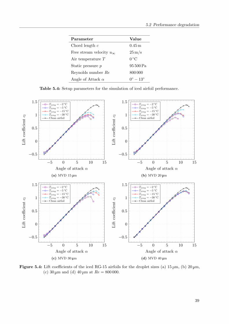
5.2 Performance degradation

Parameter Value

Chord length c 0.45 m

Free stream velocity u∞ 25 m/s

Air temperature T 0 ◦C

Static pressure p 95 500 Pa

Reynolds number Re 800 000

Angle of Attack α 0◦ − 13◦

Table 5.4: Setup parameters for the simulation of iced airfoil performance.

−5 0 5 10 15

−0.5

0

0.5

1

1.5

Angle of attack α

Lif

tco

effici

entc l

Ticing = −2 ◦CTicing = −5 ◦CTicing = −15 ◦CTicing = −30 ◦CClean airfoil

(a) MVD 15µm

−5 0 5 10 15

−0.5

0

0.5

1

1.5

Angle of attack α

Lif

tco

effici

entc l

Ticing = −2 ◦CTicing = −5 ◦CTicing = −15 ◦CTicing = −30 ◦CClean airfoil

(b) MVD 20µm

−5 0 5 10 15

−0.5

0

0.5

1

1.5

Angle of attack α

Lif

tco

effici

entc l

Ticing = −2 ◦CTicing = −5 ◦CTicing = −15 ◦CTicing = −30 ◦CClean airfoil

(c) MVD 30µm

−5 0 5 10 15

−0.5

0

0.5

1

1.5

Angle of attack α

Lif

tco

effici

entc l

Ticing = −2 ◦CTicing = −5 ◦CTicing = −15 ◦CTicing = −30 ◦CClean airfoil

(d) MVD 40µm

Figure 5.4: Lift coefficients of the iced RG-15 airfoils for the droplet sizes (a) 15 µm, (b) 20 µm,(c) 30 µm and (d) 40 µm at Re = 800 000.

39

5 Ice accretion results and performance degradation

−5 0 5 10 150

0.02

0.04

0.06

0.08

0.1

0.12

0.14

Angle of attack α

Dra

gco

effici

entc d

Ticing = −2 ◦CTicing = −5 ◦CTicing = −15 ◦CTicing = −30 ◦CClean airfoil

(a) MVD 15 µm

−5 0 5 10 150

0.02

0.04

0.06

0.08

0.1

0.12

0.14

Angle of attack α

Dra

gco

effici

entc d

Ticing = −2 ◦CTicing = −5 ◦CTicing = −15 ◦CTicing = −30 ◦CClean airfoil

(b) MVD 20µm

−5 0 5 10 150

0.02

0.04

0.06

0.08

0.1

0.12

0.14

Angle of attack α

Dra

gco

effici

entc d

Ticing = −2 ◦CTicing = −5 ◦CTicing = −15 ◦CTicing = −30 ◦CClean airfoil

(c) MVD 30 µm

−5 0 5 10 15

0.02

0.04

0.06

0.08

0.1

Angle of attack α

Dra

gco

effici

entc d

Ticing = −2 ◦CTicing = −5 ◦CTicing = −15 ◦CTicing = −30 ◦CClean airfoil

(d) MVD 40µm

Figure 5.5: Drag coefficients of the iced RG-15 airfoils for the droplet sizes (a) 15 µm, (b) 20 µm,(c) 30 µm and (d) 40 µm at Re = 800 000.

the entire range of AoAs. The maximum deterioration of lift and increase of drag is found at−2 ◦C / MVD 20. In this case the maximum lift coefficient decreases by 35 % and the respectivedrag increases by 160 %, compared to the clean airfoil. Additionally, the simulations show thatthe degradation of aerodynamic performance is a function of the AoA. The most likely reason forthis behavior is the flow separation at the leading edge, induced by the ice. This leading edge flowseparation occurs in glaze ice cases already at low angles of attack due to the irregular ice shapeand leads to a loss of lift, whereas the airflow at the leading edge of the clean airfoil and iced airfoilin rime ice cases with a streamline shape is still fully attached. Fig. 5.6 demonstrates this behavior.While the clean airfoil and the rime ice case at −30 ◦C / MVD 20 still show a fully attached flowat the leading edge, but a much thicker boundary layer at the rime ice case, the glaze ice case at−2 ◦C / MVD 20 already contains flow separation. With increasing AoA the area of separated flow

40

5.2 Performance degradation

(a) Clean airfoil / AoA 2◦ (b) −30 ◦C / MVD 20 / AoA 2◦

(c) −2 ◦C / MVD 20 / AoA 2◦ (d) −2 ◦C / MVD 20 / AoA 6◦

Figure 5.6: Airflow around the RG-15 leading edge at an AoA of 2◦ for (a) the clean airfoil, (b)the −30 ◦C / MVD 20 icing condition, (c) the −2 ◦C / MVD 20 icing condition and(d) the −2 ◦C / MVD 20 icing condition at an AoA of 6◦.

at the leading edge increases, as shown in Fig. 5.6d, which amplifies the loss of lift and extends thedeviation between iced airfoil and clean airfoil results. The fully turbulent airflow setup might be afurther factor for the small differences of lift coefficients at small angles of attack. If the iced airfoilwould,in reality, show small laminar separation of flow at the leading edge due to the ice, the fullyturbulent initialized boundary layer flow acts as an artificial turbulator, stabilizing the airflow andpossibly preventing any separation of airflow in the simulation which could ultimately lead to theprediction of higher lift coefficients.

This explanation also shows an uncertainty of this work. All simulations that include ice are setup with a fully turbulent boundary layer, since an immediate transition from laminar to turbulentis expected, due to the high surface roughness of the ice. However, it has not been verified if thisassumption is correct or if iced airfoils still show at least a partially laminar airflow. This couldlead to different results for the iced airfoil performance. Although the validation results for thesimulation of ice accretion did show good agreement to the experimental results in this work, itmay be advised that future work includes laminar airflow in the ice accretion simulation. At leastin the first step of the simulation, where no ice is on the airfoil yet, a laminar flow could yield

41

5 Ice accretion results and performance degradation

0 0.2 0.4 0.6 0.8 1

−10

−5

0

Dimensionless x-coordinate x/c

Pre

ssu

reco

effici

entc p

α = 0◦

α = 4◦

α = 6◦

α = 8◦

α = 12◦ (cl max)

(a) Clean airfoil

0 0.2 0.4 0.6 0.8 1

−10

−5

0

Dimensionless x-coordinate x/c

Pre

ssu

reco

effici

entc p

α = 0◦

α = 4◦

α = 6◦

α = 8◦

α = 12◦ (cl max)

(b) −30 ◦C / MVD 40

0 0.2 0.4 0.6 0.8 1

−3

−2

−1

0

1

Dimensionless x-coordinate x/c

Pre

ssu

reco

effici

entc p

α = 0◦

α = 4◦

α = 6◦

α = 8◦ (cl max)

(c) −2 ◦C / MVD 20

0 0.2 0.4 0.6 0.8 1

−10

−5

0

Dimensionless x-coordinate x/c

Pre

ssu

reco

effici

entc p

Clean α = 8◦

−30 ◦C / MVD 40 α = 8◦

Clean α = 12◦

−30 ◦C / MVD 40 α = 12◦

(d) Clean airfoil vs. −30 ◦C / MVD 40

Figure 5.7: Pressure distribution on the RG-15 at various angles of attack for (a) the clean airfoil,(b) the icing condition −30 ◦C / MVD 40, (c) −2 ◦C / MVD 20 and (d) a comparisonof (a) and (b) at the AoAs 8◦ and 12◦.

better results. Additionally, previous work by Hann [20] has indicated, that a turbulent flow mayincrease the evaporation rate and leads to earlier disappearance of water layers compared to laminarconditions. This implies that ice accretion simulations that consider laminar flow could lead to moresevere ice shapes compared to simulations that are set up with a fully turbulent boundary layer. Italso points out the importance to investigate flow transition on iced airfoils not only to gain betterknowledge about the impact on the ice accretion process and the aerodynamic performance, butalso to successfully define energy requirements for an icing protection system.

Comparing the lift and drag results of all icing conditions, the curves show a strong correlationbetween the aerodynamic performance and the iced airfoil’s shape. For streamline shaped ice (e.g.ice shapes at an MVD of 40 µm), the simulation predicts smaller decrease of lift and increase of

42

5.2 Performance degradation

drag, compared to icing cases with rough surfaces and a larger ice shape extension in y-direction(e.g. MVD 15, 20 and 30 at −2 ◦C icing temperature). The distribution of pressure coefficients givesfurther insight to this behavior. In Fig. 5.7 the pressure coefficient distribution of the clean airfoil,the least severe rime ice condition at −30 ◦C / MVD 40 and the worst case glaze ice conditionat −2 ◦C / MVD 20 are shown at several AoAs. The results clearly show that for rime ice witha very streamline shaped geometry the overall pressure distribution is similar to the clean airfoil.The direct comparison of the clean airfoil to the rime ice condition at an 8◦, shown in Fig. 5.7d,reveals only slightly reduced pressure coefficients for the rime ice case around the leading edge.Further aft areas show no considerably different pressure coefficients. At the stall angle of 12◦ thedifference between clean and iced airfoil has increased, explaining the small reduction of maximumlift coefficient for this icing condition, but the general distribution of pressure still matches the cleanairfoil. The glaze ice case on the other hand reveals a significantly disturbed airflow situation aroundthe leading edge, where ice is present. The irregular surface results in very turbulent and separatedflow at the bumps which prevents the conformation of larger pressure coefficients, especially on thesuction side of the airfoil. Further, the effect of the previously mentioned separation of flow at theleading edge can be observed at the change from α = 6◦ to α = 8◦. Due to already separated flow,the increase of angle of attack does not lead to larger pressure coefficients, restricting the maximumpossible lift coefficient in this conditions. The higher values at the trailing edge at an angle of attackof α = 8◦ compared to lower AoAs are considered unrealistic, since the AoA of 8◦ already includesseparation of flow on the suction side at the trailing edge, marking the begin of the stall.

Another effect of icing can be seen in Fig. 5.4: Additionally to the decreased maximum lift coefficient,icing results in a decreasing stall angle. With both parameters decreased due to icing, the airfoiloffers a more critical stall behavior considering for example that the aircraft is flown by an autopilotbased on the envelope of the clean airfoil. A possible explanation for the stall at smaller AoAs isthe leading edge flow separation on severely iced airfoils. With larger angles of attack the area ofseparated flow, due to the ice, increases and ultimately fails to reattach at smaller AoAs leading tothe stall, whereas the airflow is still attached at the leading edge of the clean airfoil and streamlineice shapes. This would also explain the observation that the greatest degradation of the stall angleoccurs at a glaze ice case at −2 ◦C / MVD 20, whereas less severe rime ice shapes revealed smallerchanges of the stall angle. For the maximum investigated droplet size of 40 µm which contains iceshapes close to the clean airfoil geometry, the results show no change of the stall angle at all. Inreality it is suspected that even at this droplet size icing has an effect on the stall angle, although thedifference to the clean airfoil might be very small. Considering stall angle changes, the simulationsetup limits the validity of the results. With a setup of AoA steps of 1◦ and the stall angle of theclean airfoil identified at AoA 12◦, the minimum resolution for the stall angle that can be capturedby the simulation is approx. 8.5 %. Any change of stall angle below 8.5 % can not be captured bythe simulation. Thus, the results show the general influence of icing on the stall angle, but if a moreprecise information on the stall angle is desired, more simulations at smaller AoA steps are requiredin the stall region.

Apart from lift and drag coefficient, the moment coefficient over the AoA for the iced airfoilsis presented in Fig. 5.8. The curves show that icing increases the moment gradient in all icingcases. As for lift and drag, higher temperatures in combination with high LWC values show greaterinfluence on the moment, compared to lower temperatures and low LWC values. Regarding theflight mechanics, the increased airfoil moment at common AoAs between 0◦ and 5◦ correspondsto a reduced nose down moment of the airfoil. Since the overall aircraft’s moment gradient mustbe ∂cm/∂α < 0 for longitudinal static stability, all icing cases reduce this stability at first sight.However, further aircraft parameters such as the general aircraft configuration and possible icing of

43

5 Ice accretion results and performance degradation

−5 0 5 10 15

−0.08

−0.06

−0.04

−0.02

0

0.02

Angle of attack α

Mom

ent

coeffi

cien

tc m

Ticing = −2 ◦CTicing = −5 ◦CTicing = −15 ◦CTicing = −30 ◦CClean airfoil

(a) MVD 15µm

−5 0 5 10 15

−0.06

−0.04

−0.02

0

Angle of attack α

Mom

ent

coeffi

cien

tc m

Ticing = −2 ◦CTicing = −5 ◦CTicing = −15 ◦CTicing = −30 ◦CClean airfoil

(b) MVD 20µm

−5 0 5 10 15−0.1

−0.08

−0.06

−0.04

−0.02

0

0.02

Angle of attack α

Mom

ent

coeffi

cien

tc m

Ticing = −2 ◦CTicing = −5 ◦CTicing = −15 ◦CTicing = −30 ◦CClean airfoil

(c) MVD 30µm

−5 0 5 10 15

−0.06

−0.05

−0.04

−0.03

−0.02

−0.01

Angle of attack α

Mom

ent

coeffi

cien

tc m

Ticing = −2 ◦CTicing = −5 ◦CTicing = −15 ◦CTicing = −30 ◦CClean airfoil

(d) MVD 40µm

Figure 5.8: Moment coefficients of the iced RG-15 airfoils for the droplet sizes (a) 15 µm, (b)20 µm, (c) 30 µm and (d) 40 µm at Re = 800 000.

the horizontal stabilizer or even the elevator must be considered to identify possible dangers on theaircraft’s overall longitudinal stability. Therefore, no statement about absolute aircraft stability canbe made, based on this results. Considering only the effect on the airfoil, icing changes the momentbehavior from almost constant for −5◦ ≤ α ≤ 5◦ to a positive gradient. This includes a reducednose down moment for α ≥ −1◦.

5.2.2 Index visualization

In order to create a better overview over the different impacts of icing on the aerodynamicperformance for all icing cases, an index for the lift, drag, stall AoA and the moment shall be

44

5.2 Performance degradation

introduced at this point. Three discrete points are representing the iced airfoil performance for liftand drag in comparison to the clean airfoil:

AoA 0 ◦: Smallest changes in drag compared to the clean airfoil and minor changes in lift

AoA 6 ◦: Start of increasing airfoil moment

Stall angle: Maximum spread between iced and clean airfoil

For the moment index, two different discrete points are chosen:

AoA 0 ◦: Small changes in moment compared to the clean airfoil

AoA 4 ◦: Limit of the linear AoA range of the clean airfoil – maximum spread to the cleanairfoil

For the stall angle index, the calculation consists only of the angle of attack to which the maximumlift coefficient corresponds. The index for lift, drag, moment and stall angle is calculated with thefollowing equations:

Ilift,drag =1

3

[∆Cl stall

∆Cl stall max+

∆Cl α0∆Cl α0 max

+∆Cl α6

∆Cl α6 max

](5.1)

Imoment =1

2

[∆Cl α0

∆Cl α0 max+

∆Cl α4∆Cl α4 max

](5.2)

Istall angle =∆αstall

∆αstall max(5.3)

All max-values (denominators) represent the difference between the clean airfoil value and theworst-case performance within all icing cases for the certain AoA. The numerator values are thedifference between the clean airfoil performance and the respective value of the current icing case.As a result, the fractions and the overall index can result in values between 0 and 1. An indexvalue of 1 represents the maximum performance degradation, as maximum deterioration of lift ormaximum increase in drag or moment, whereas a value of 0 would indicate no difference to theclean airfoil performance.

Figure 5.9 shows the index distribution for the complete range of investigated meteorologicalconditions as a color value. The index values of the areas between the actually investigated icingconditions are determined with a piecewise bi-linear interpolation. Therefore, the overall parametricspace is distributed into smaller areas, each limited by four investigated conditions. The indexvalue is interpolated across each face, based on the discrete values at the corners. This approachprovides a valuable insight on the influence of various meteorological conditions on the aerodynamicperformance which was the intention of this work. It visualizes how severe different icing conditionsare in comparison to each other and where to expect worst-case icing conditions.

The results for the lift and drag coefficient clearly show that the worst performance degradationcan be found at temperatures close to 0 ◦C to which a high liquid water contents corresponds andgenerally smaller droplet sizes. The most uncritical conditions are identified at generally low LWCat low temperatures and large droplet sizes. The results further show that low temperatures, towhich low LWC values correspond, have only small impact on the performance independently fromthe droplet size. At temperatures close to freezing however, different droplet sizes contain a largerrange of LWC and therefore show different impact on the performance, depending on the prevailingMVD. The index visualization for the moment shows a distribution closely related to the one for

45

5 Ice accretion results and performance degradation

15 20 25 30 35 400

0.2

0.4

0.6

0.8

Air temp. -2°C

-10°C

-20°C-30°C

0

0.2

0.4

0.6

0.8

1

(a) Index - Lift coefficient

15 20 25 30 35 400

0.2

0.4

0.6

0.8

Air temp. -2°C

-10°C

-20°C-30°C

0

0.2

0.4

0.6

0.8

1

(b) Index - Drag coefficient

15 20 25 30 35 400

0.2

0.4

0.6

0.8

Air temp. -2°C

-10°C

-20°C-30°C

0

0.2

0.4

0.6

0.8

1

(c) Index - Moment coefficient

15 20 25 30 35 400

0.2

0.4

0.6

0.8

Air temp. -2°C

-10°C

-20°C-30°C

0

0.2

0.4

0.6

0.8

1

(d) Index - Stall angle

Figure 5.9: Index visualization of the RG-15 airfoil performance degradation for (a) lift, (b) drag,(c) moment coefficient and (d) stall angle.

lift and drag. The most severe icing conditions that result in highest lift reduction and highest dragincrease also show the largest increase of the moment. The overview for the stall angle shows adistribution closely related to the one for lift, drag and moment coefficients. At small droplet sizeshowever, the simulations predict similar changes to the stall angle for all four different temperatures,whereas for the lift, drag and moment lower temperatures show less impact on the performance.Again as previously mentioned, the validity of data regarding the stall angle is limited due to theresolution of angles of attack. The results still give a good first insight to the general influence ofdifferent weather conditions on the stall angle.

5.3 Uncertainties and future work

Besides the discussion of results in the previous sections, at this point, further uncertainties of thiswork shall be discussed with regard to future work on this topic.

46

5.3 Uncertainties and future work

None of the simulation results for both ice accretion and performance have been validated byexperimental data. The validation results show strong indications that the simulation modelis capable of capturing the ice accretion process and the airfoil performance for different icingconditions correctly. However, due to the lack of experimental data at higher Reynolds numbersthe validation results still contain limitations, because the relation of inertia to viscous forces isdifferent for the validation data, which affects the modeling of the boundary layer and ultimatelythe calculation of aerodynamic forces. Additional wind tunnel tests would be necessary to validatethe simulation results of this work, especially with regard to the specific Reynolds number and thedeviation between simulation and wind tunnel results that has been found within the validationof the iced airfoil performance prediction (ref. to Fig. 4.5 in Sec. 4.2.2). The experimental datain comparison to the simulation results would also give further insight on the suitability of theSA turbulence model to predict the aerodynamic performance for severely iced airfoils. Regardingthe fully turbulent boundary layer setup for iced airfoils in this work, the wind tunnel tests couldprovide new information, if laminar flow should be considered for the simulations and how large theeffect of not considering laminar flow is.

Regarding the simulation of ice accretion, only a monodisperse droplet size distribution and the iceaccretion process at only one angle of attack of 0 ◦ are considered. A monodisperse distribution ofdroplet sizes is not likely to be found in reality. The Advisory Circular No 20-73A from the FAAsuggests using a Langmuir-D distribution for droplet sizes up to 50 µm for the icing certification ofmanned aircraft [11]. Since FENSAP-ICE already provides the Langmuir-D distribution withinDROP3D, further simulations using the FAA’s suggested distribution could give insight on the effectof differently distributed droplet sizes. Also a constant AoA of 0 ◦ is not realistic for a stationaryflight. An actual average AoA for stationary horizontal flight or even a dynamically changing AoAfor a specific flight mission would consider different airflow situations on the airfoil. This wouldsubsequently influence the ice accretion process and might yield more realistic ice shapes. Therefore,more extensive tests in icing wind tunnels and flight tests in icing conditions could provide usefuldata on the evaluation of the accuracy of the ice accretion simulation model.

Evaluating a two dimensional airfoil instead of a complete three dimensional wing, enabled theinvestigation of 16 different icing conditions at the given time frame. Especially the computationalcosts for the simulation of ice accretion are increasing significantly for a large 3D wing, due tothe fine grid resolution that is required around the leading edge. However, this setup includescommon limitations that are involved for a 2D airfoil investigation. In terms of drag this means,only frictional forces and form drag is considered but no induced drag. An icing simulation of a 3Dwing and a comparison to the results of this work could be used to study possible effects of icing onthe induced drag and might provide new information to improve the accuracy of numerical methodsto predict icing effects.

Finally, the evaluation of iced airfoil performance mainly concentrates on positive AoAs up to thestall at high AoAs. Depending on the design of the UAV and it’s operational flight envelope aninvestigation of negative AoAs and stall at negative AoAs might be of interest. If additionally aprecise prediction of the stall angle is desired, further simulations with smaller steps of AoA arerequired to increase the resolution of results near the maximum lift coefficient.

These uncertainties show that precise validation of the simulation models with suitable experimentaldata, the investigation about a possible influence of laminar flow and the consideration of furthermeteorological characteristics, such as droplet size distribution, are the main challanges for futurework in order to increase the fidelity of the numerical data. Subsequently, the refined simulationmodels could be used to focus more on the effect of icing in critical icing conditions to increase the

47

5 Ice accretion results and performance degradation

resolution of results in this area. Due to the aim of covering a large range of icing conditions, thiswork probably only partially represents the most critical meteorological conditions.

5.4 Relevance of the simulation results for an IPS development

After the presentation and discussion of the results, this section is intended to point out the relevanceof the findings of this work for the development of a icing protection system for small fixed-wingUAVs.

The knowledge about the influence of different icing conditions on the aerodynamic performancecan be used for the adaptation of flight controllers and control systems of icing protection systems.Based on the results for lift, drag, moment and stall angle, flight controllers could adapt the flightenvelope according to the present icing conditions to maximize the aircraft’s aerodynamic efficiency.In terms of adapting IPS control systems, the results provide useful information to maximize energyefficiency for example of a promising concept for an electro-thermal icing protection system withfully autonomous icing detection for UAVs, presented in [38] and [22]. The icing detection systemoperates intermittently to detect possible ice accretion. With the additional information on theinfluence of different icing conditions, the ice detection frequency could be reduced in less criticalconditions to save electrical energy.

Further, the identification of a worst-case icing condition at −2 ◦C / MVD 20 can be used for thedesign process of an IPS system. With the meteorological conditions that lead to the greatestperformance degradation further simulations and wind tunnel tests can be conducted to determinethe maximum heat flux of the icing protection system that is required to protect the airfoil inworst-case icing conditions. Additionally, as stated in [20], the identification of the critical icingdesign cases is an important task for the development of an UAV IPS. With the worst-case icingcondition identified at −2 ◦C / MVD 20 and the knowledge about the severity of various icingconditions this study provides new information that can be used in the decision process on whenand how to operate the IPS. This includes either operating the IPS running wet, which allows liquidwater on the surface, or fully evaporative where no liquid water remains on the surface and alsoif the IPS is operated as anti-icing system that prevents icing completely or de-icing system thatallows some accretion of ice before being removed.

The implementation of the current results in the development process of an IPS is an importanttask for the future, since it helps identifying where further and/or more precise data are requiredto successfully define the IPS requirements and realize them. This would for example providenew information about how many additional icing conditions need to be investigated to reach asufficient database for a successfull IPS development. It would also reveal what customizations orsupplementary investigations are required to apply the results to a specific UAV, other than thePX-31.

48

6 Conclusion

In this work, a large parameter study has been performed in order to investigate the influence ofdifferent meteorological conditions on the aerodynamic performance of a UAV airfoil. Therefore,CFD simulations were used to predict the ice accretion and the aerodynamic performance of a 2Dairfoil. The investigated airfoil is the RG-15 laminar airfoil that is used by the PX-31, a fixed wingUAV with 3.2 m wingspan.

In total, 16 different icing conditions have been investigated. The conditions largely cover an icingenvelope by the Federal Aviation Administration in CFR 14, Part 25, App. C that applies tothe certification of large aircraft. Generally, these FAA requirements include two different icingenvelopes, applicable for intermittent and continuous icing at different cloud ceiling heights. Theenvelope used within this work applies for cloud ceiling heights from 22 000 ft (6 700 m) down to sealevel, thus including low flight altitudes of small UAVs. Each of the 16 icing conditions is definedby the droplet size, the median volume diameter and the air temperature to which a liquid watercontent corresponds. Four different temperatures at four different droplet sizes are investigated,covering a a temperature range of −30 ◦C to −2 ◦C, a median volume diameter range of 15 µmto 40 µm and the corresponding liquid water content of 0.038 g/m3 to 0.760 g/m3. The icingduration for all icing conditions is set to 21.5 min, considering the cruising speed of the PX-31 UAVand the maximum horizontal cloud extend, which is also defined in the FAA requirements.

For all simulations, ANSYS FENSAP-ICE (version 2019 R1) software was used. The process ofice accretion is calculated by the three modules FENSAP, DROP3D and ICE3D of FENSAP-ICE.FENSAP is the CFD solver that acquires the airflow solution. DROP3D calculates the distributionof water on the airfoil’s surface, based on the airflow solution and ICE3D determines the ice accretionbased on the FENSAP and DROP3D results and creates a new grid that includes the ice geometry.For the whole icing duration the three modules run in multiple loops. Thereby, ice on the airfoilfrom previous loops is considered for the following calculations of the airflow solution by FENSAP.For the subsequent calculation of aerodynamic performance, only the FENSAP module was used ina second simulation model.

For all simulations, FENSAP was set up to calculate the steady flow solution by solving compressibleReynolds averaged Navier-Stokes (RANS) equations. Turbulence is modeled by the one-equationSpalart-Allmaras model. The boundary layer was set up fully turbulent for simulations that includeice on the airfoil. Only for simulations of the clean airfoil laminar flow with fixed transition locationwas initialized. XFOIL was used for obtaining the transition locations. For the validation of theaerodynamic performance of the clean airfoil one additional simulation has been performed withthe k-ω-SST and a local correlation-based intermittency transition model to compare the results ofthe two different turbulence models.

The numerical grids were created with Pointwise (version 18.2). For the simulation of clean andiced airfoil performance two grid dependency studies have been performed, to ensure independenceof the aerodynamic coefficients from the grid resolution. For the simulation of ice accretion insteadof a grid dependency study a timestep-study was performed, since the focus was not on precise

49

6 Conclusion

calculation of aerodynamic coefficients, but on capturing the ice shapes correctly. Therefore, thenumber of loops of the previously presented modules was varied in order to evaluate the differentresulting geometries. With regard to the geometry output and the simulation time, a setup with 15steps, where the first step covers 30 s and the following 14 steps cover 90 s each, was chosen.

Both simulation models were validated with literature data of wind tunnel tests. The simulationresults for the ice accretion were compared to experimental data of two different icing conditions,rime ice at −15 ◦C / MVD 20 µm and glaze ice at −2 ◦C / MVD 30 µm. These specific conditionswere selected because they show completely different shapes. Rime ice at low temperatures ischaracterized by a streamlined shape and a rough surface, where all impinging ice freezes instantly,whereas glaze ice at temperatures close to freezing shows an irregular but smoother surface withicing limits further back on the airfoil, due to water that does not freeze instantly and runs backon the surface before freezing. The simulation showed good capability of capturing the general iceshape at the different icing conditions. The numerical results further showed good agreement tothe experimental data for the icing limit on the lower surface of the airfoil and the ice extend inx-direction. On the upper surface, the simulation predicted the icing limits further towards theleading edge compared to the wind tunnel tests in both cases. It is expected that this has an influenceon the aerodynamic performance results of numerical data in comparison to the experiments butis accepted, since the numerical calculation enables a cheaper opportunity to investigate a largenumber of icing conditions, whereas wind tunnel tests are more expensive.

The simulation results for the prediction of aerodynamic performance were compared to wind tunneldata of a clean and an iced airfoil. In case of the iced airfoil, no suitable data could be found foran iced RG-15 airfoil, hence wind tunnel data for an iced NREL S826 airfoil at a low Reynoldsnumber of Re = 400 000 were used. The simulation results for the clean airfoil revealed goodagreement to the experimental data. The two different turbulence models showed small differencesat high angles of attack in their stall prediction. The SA model predicts a higher maximum liftcoefficient at a higher stall angle compared to the k-ω-SST model, but both within close range tothe experimental results. The drag results confirmed good fit of both simulations with the windtunnel data. Again differences between the turbulence models could be seen at AoAs >7◦, wherethe k-ω-SST model predicts higher drag as the SA model. For the iced airfoil the simulation resultsfit to the experimental results for small AoAs but deviate for larger AoAs, where the simulationpredicts a lower lift gradient and lower maximum lift coefficient. Also the drag is under-predictedfor all AoAs by the simulation, but the general behavior over the complete AoA range is similar tothe experimental results. The high turbulence intensity and large flow separations at the leadingedge due to the very severe icing case with ice horns in combination with the SA turbulence modelis suspected to be the reason for the diverging results. However, the simulation showed goodconvergence behavior at all AoAs and no indication that an unsteady flow solution is required.Therefore no final explanation for this deviation was found. Since the ice shapes of the all 16conditions of this study did not show that severe icing and no horn protrusions, less significantflow separations at the leading edge were expected and the results of the simulation model wereconsidered acceptable.

After the validations, the ice accretion was simulated for all 16 different icing conditions. Thesimulations show the largest ice masses for glaze ice cases at temperatures close to freezing thatinclude high amounts of liquid water. The overall highest ice mass was found at a temperatureof -2 ◦C and a droplet MVD of 20 µm. Lower temperatures result in more streamline shaped iceand lower masses. At the largest investigated droplet size of 40 µm all temperatures, even close tofreezing lead to rime ice with a streamlined shape and the lowest ice masses. The reason therefore is

50

that increasing droplet sizes can only contain a decreasing range of liquid water content accordingto the icing envelope. At the largest droplet size the LWC has decreased to a value where all waterfreezes instantly on impact.

Based on the ice accretion results, the aerodynamic performance was simulated for all iced airfoilsand compared to the clean airfoil performance. The results showed that icing decreases the maximumlift coefficient and increases drag and airfoil moment in all icing conditions. The greatest degradationof performance was found for glaze ice cases with rough and uneven surfaces that disturb the airflowthe most. The glaze ice cases also include the greatest reduction of the stall angle, whereas icingcases with a very streamlined shape show only small to no reduction of the stall angle. For abetter overview of the influence of the different meteorological conditions, a dimensionless index,representing the performance degradation, was introduced. It is defined by the difference of lift,drag, airfoil moment and stall angle of the iced airfoils to the clean airfoil for several angles ofattack to cover a larger range of AoAs. The index includes values from zero to one, where a valueof one indicates the maximum degradation found within all 16 icing conditions and a value of zeroindicates no change to the clean airfoil performance. The index values are then interpolated viabi-linear interpolation between all investigated conditions to give an estimated influence of thecomplete range of conditions. This index visualization showed that the most critical icing conditionscan be expected at high liquid water contents that correspond to temperatures close to zero andsmaller droplet sizes. The worst case performance degradation was identified at -2 ◦C / 40 µm, thesame condition that lead to the highest ice mass. The overview also shows, that icing conditions atlow temperatures and low LWC values, independently from the prevailing droplet size, have onlylittle impact on the aerodynamic performance.

Regarding the development of an icing protection system (IPS) for small fixed-wing UAVs, theseresults provide important new information. The worst case icing condition can be used for furthersimulations and wind tunnel tests to determine the maximum heat flux that is required for anelectro-thermal IPS system to de-ice the airfoil in the most severe icing conditions. Additionallyan automatic intermittently operating icing detection system can use the knowledge on where toexpect worse or less severe icing conditions to reduce the frequency with which icing is detected tooptimize the energy consumption of the system.

51

Bibliography

[1] UBIQ Aerospace: D·ICE. https://www.ubiqaerospace.com/ [Online, accessed 2019-06-23].

[2] Lorenzo Battisti: Wind Turbines in Cold Climates - Icing Impacts and Mitigation Systems.Springer International Publishing, 2015.

[3] H. Beaugendre, F. Morency and W. G. Habashi: Development of a Second GenerationIn-Flight Icing Simulation Code. In: Journal of Fluids Engineering, Vol. 128, 2006, pp. 378–387.

[4] Y. Bourgault, H. Beaugendre and W. G. Habashi: Development of a Shallow-WaterIcing Model in FENSAP-ICE. In: Jounal of Aircraft, Vol. 37, 2000, pp. 640–646.

[5] Y. Bourgault, Z. Boutanios and W. G. Habashi: Three-Dimensional Eulerian Approachto Droplet Impingement Simulation Using FENSAP-ICE, Part 1: Model, Algorithm, andValidation. In: Journal of Aircraft, Vol. 37, 2000, pp. 9.

[6] Y. Bourgault, Z. Boutanios and W. G. Habashi: FENSAP-ICE’s Three-DimensionalIn-Flight Ice Accretion Module: ICE3D. In: Journal of Aircraft, Vol. 40, 2003, pp. 239–247.

[7] Y. Bourgault, W. G. Habashi, J. Dompierre and G. S. Baruzzi: A finite elementmethod study of Eulerian droplets impingement models. In: International Journal for NumericalMethods in Fluids, Vol. 29, 1999, pp. 4.

[8] M. B. Bragg, A. P. Broeren and L. A. Blumenthal: Iced-airfoil aerodynamics. In:Progress in Aerospace Sciences, Vol. 41, 2005, pp. 323–362.

[9] L. Brandrud and L. Krøgenes: Aerodynamic Performance of the NREL S826 Airfoil inIcing Conditions. Master’s thesis, Norwegian University of Science and Technology (NTNU),2017.

[10] M. Drela: XFOIL: An Analysis and Design System for Low Reynolds Number Airfoils. MITDept. of Aeronautics and Astronautics, Cambridge, Massachusetts, 1989.

[11] Federal Aviation Administration (FAA): Aircraft Icing Protection. Advisory Circular20-73A, 2006.

[12] Federal Aviation Administration (FAA): Part I - Atmosphreic Icing Conditions. Title14 CFR Subchapter C Part 25 Appendix C, No. 4080, 29 FR 17955, Amdt. 25-140, 79 FR65528, November 2014.

[13] Federal Aviation Administration (FAA): Pilot Guide: Flight in Icing Conditions. Advi-sory Circular, No. AC 91-74B, October 2015.

[14] R. Fiolka: F3B - The optimization of different flying states.http://www.teamusaf3b.com/what-is-f3b/f3b-the-optimization-of-different-flying-states[Online, accessed 2019-06-23].

53

Bibliography

[15] R. W. Gent, N. P. Dart and J. T. Cansdale: Aircraft icing. In: Philosophical Transactionsof the Royal Society A Mathematical, Physical and Engineering Sciences, Vol. 358, November2000, pp. 2873–2911.

[16] NTNU HPC Group: Vilje HPC cluster system. https://www.hpc.ntnu.no/display/hpc/About-+Vilje [Online, accessed 2019-07-29].

[17] SAE International Group: Icing Wind Tunnel Interfacility Comparison Tests. AerospaceInformation Report AIR5666, SAE Aerospace, 2012.

[18] W. G. Habashi, F. Morency and H. Beaugendre: FENSAP-ICE: A Second Generation3D CFD-based In-Fligh Icing Simulation System. SAE Technical Paper 2003-01-2157, 2003.

[19] R. Hann: UAV Icing: Comparison of LEWICE and FENSAP-ICE for Ice Accretion andPerformance Degradation. In: 2018 Atmospheric and Space Environments Conference, Atlanta,Georgia, June 2018.

[20] R. Hann: UAV Icing: Comparison of LEWICE and FENSAP-ICE for Anti-Icing Loads. In:AIAA SciTech Forum, 2019.

[21] R. Hann: UAV Icing: Ice Accretion Experiments and Validation. SAE Technical Paper2019-01-2037, SAE International Conference on Icing of Aircraft, Engines, and Structures,2019.

[22] R. Hann, K. Borup, A. Zolich, K. Sørensen, H. Vestad, M. Steinert and T. A.Johansen: Experimental Investigations of an Icing Protection System for UAVs. TechnicalReport 2019-01-2038, SAE International, 2019.

[23] R. Hann, J. Krøgenes, L. Brandrud, J. Bartl, T. Bracchi and L. Sætran: Experi-mental and Numerical Investigation of Icing Penalties of a UAV and Wind Turbine Airfoil atLow Reynolds Numbers. 2019. unpublished manuscript.

[24] ANSYS Inc.: ANSYS FENSAP-ICE User Manual, Southpointe 2600 ANSYS Drive Canons-burg, PA 15317, Release 18.2, August 2017.

[25] International Civil Aviation Organization: Manual of the ICAO Standard Atmosphere,Release 3, 1993.

[26] G. G. Koenig, C. C. Ryerson and R. Kmiec: UAV Icing Flight Simulation. In: 40thAIAA Aerospace Science Meeting and Exhibit, no. AIAA-2002-0812, Reno, Nevada, Januar2002.

[27] P. Lindamae, C. C. Reyerson and J. Martel: Army Aircraft Icing. Technical ReportERDC/CRREL TR-02-13, US Army Corps of Engineers, September 2002.

[28] B. L. Messinger: Equilibrium Temperature of an Unheated Icing Surface as a Function ofAir Speed. In: Jounal of the Aeronautical Sciences, Vol. 20, 1953, pp. 29–42.

[29] F. Morency: Anti-Icing System Simulation Using CANICE. In: Journal of Aircraft, Vol. 36,1999, pp. 999–1006.

[30] F. Morency, H. Beaugendre, G. S. Baruzzi and W. G. Habashi: FENSAP-ICE: AComprehensive 3D Simulation System for In-flight Icing. In: 15th AIAA Computational FluidDynamics Conference, no. 2001-2566, 2001.

[31] NASA: Ice on Power Forced Model Rotor. https://www1.grc.nasa.gov/wp-content/uploads/C95 03918.jpg [Online, accessed 2019-04-12].

54

Bibliography

[32] Maritime Robotics: Multipurpose UAS. https://maritimerobotics.com/as-px-31/ [Online,accessed 2019-06-15].

[33] Dieter Sartorius: Hitzdrahtmessungen zur Grenzschicht- und Nachlaufentwicklung beiAbloseblasen in der Nahe der Profilhinterkante. Diplomarbeit, Stuttgart, July 2001.

[34] Rudiger Schwarze: CFD-Modellierung. Springer Vieweg, 2013.

[35] Michael S. Selig, James J. Guglielmo, Andy P. Broeren and Philippe Giguere:Summary of Low-Speed Airfoil Data. Vol. 1, SoarTech Publications, 1995.

[36] R. A. Siquig: Impact of icing on Unmanned Aerial Vehicel (UAV) Operations. TechnicalReport AD-A231 191, Naval Environmental Prediction Facility Monterey, 1990.

[37] K. L. Sørensen: Autonomous Icing Protection Solution for Small Unmanned Aircraft - AnIcing Detection, Anti-Icing and De-Icing Solution. PhD Thesis, Norwegian University of Scienceand Technology (NTNU), 2016.

[38] K. L. Sørensen and T. A. Johansen: Flight Test Results for Autonomous Icing ProtectionSolution for Small Unmanned Aircraft. In: 2017 International Conference on UnmannedAircraft Szstems (ICUAS), 2017, pp. 971–980.

[39] K. Szilder and E. Lozowski: Progress towards a 3D Numerical Simulation of Ice Accretionon a Swept Wing using the Morphogenetic Approach. SAE Technical Paper 2015-01-2162, SAEInternational, June 2015.

[40] K. Szilder and S. McIlwain: In-Flight Icing of UAVs - The Influencee of Reynolds Numberon the Ice Accretion Process. SAE Technical Paper 2011-01-2572, National Research CouncilCanada, October 2011.

[41] K. Szilder and W. Yuan: The Influence of Ice Accretion on the Aerodynamic Performanceof a UAS Airfoil. In: 53rd AIAA Aerospace Science Meeting and Exhibit, 2015.

[42] S. K. Thomas, R. P. Cassoni and C. D. MacArthur: Aircraft Anti-Icing and De-IcingTechniques and Modeling. In: Journal of Aircraft, Vol. 33, 1996.

[43] P. Tran, G. Baruzzi, F. Tremblay, P. Benquet, W. G. Habashi, P. B. Petersen,M. W. Liggett and S. Fiorucci: FENSAP-ICE applications to unmanned aerial vehicles(UAV). In: 42nd AIAA Aerospace Sciences Meeting and Exhibit, no. AIAA-2004-402, Januar2004, pp. 390–402.

[44] P. Tran, M. T. Brahimi, I. Paraschivoiu, A. Pueyo and F. Tezok: Ice Accretion onAircraft Wings with Thermodynamic Effects. In: 32nd AIAA Aerospace Sciences Meeting andExhibit, 1994.

[45] David C. Wilcox: Turbulence Modeling for CFD. DCW Industries, Inc., 1993.

55