The why, how, and when of representations for complex systems

Leo Torresleo@leotrs.com

Network Science Institute,Northeastern University

Ann S. Blevinsannsize@seas.upenn.edu

Department of Bioengineering,University of Pennsylvania

Danielle S. Bassettdsb@seas.upenn.edu

Department of Bioengineering,University of Pennsylvania

Tina Eliassi-Radtina@eliassi.org

Network Science Institute andKhoury College of Computer Sciences,

Northeastern University

February 12, 2021

1

Contents

1 Introduction 41.1 Definitions . . . . . . . . . . . . . . . . . . . . . . . . . . . . . . . . . . . . . . . . . . . . . . . 5

2 Dependencies by the system, for the system 62.1 Subset dependencies . . . . . . . . . . . . . . . . . . . . . . . . . . . . . . . . . . . . . . . . . 72.2 Temporal dependencies . . . . . . . . . . . . . . . . . . . . . . . . . . . . . . . . . . . . . . . 82.3 Spatial dependencies . . . . . . . . . . . . . . . . . . . . . . . . . . . . . . . . . . . . . . . . . 102.4 External sources of dependencies . . . . . . . . . . . . . . . . . . . . . . . . . . . . . . . . . . 11

3 Formal representations of complex systems 133.1 Graphs . . . . . . . . . . . . . . . . . . . . . . . . . . . . . . . . . . . . . . . . . . . . . . . . . 133.2 Simplicial Complexes . . . . . . . . . . . . . . . . . . . . . . . . . . . . . . . . . . . . . . . . . 153.3 Hypergraphs . . . . . . . . . . . . . . . . . . . . . . . . . . . . . . . . . . . . . . . . . . . . . 153.4 Variations . . . . . . . . . . . . . . . . . . . . . . . . . . . . . . . . . . . . . . . . . . . . . . . 163.5 Encoding system dependencies . . . . . . . . . . . . . . . . . . . . . . . . . . . . . . . . . . . 18

4 Mathematical relationships between formalisms 22

5 Methods suitable for each representation 245.1 Methods for graphs . . . . . . . . . . . . . . . . . . . . . . . . . . . . . . . . . . . . . . . . . . 265.2 Methods for simplicial complexes . . . . . . . . . . . . . . . . . . . . . . . . . . . . . . . . . . 275.3 Methods for hypergraphs . . . . . . . . . . . . . . . . . . . . . . . . . . . . . . . . . . . . . . 285.4 Methods and dependencies . . . . . . . . . . . . . . . . . . . . . . . . . . . . . . . . . . . . . 29

6 Examples 296.1 Co-authorship . . . . . . . . . . . . . . . . . . . . . . . . . . . . . . . . . . . . . . . . . . . . . 306.2 Email communications . . . . . . . . . . . . . . . . . . . . . . . . . . . . . . . . . . . . . . . . 34

7 Applications 36

8 Discussion and Conclusion 37

9 Acknowledgments 39

10 Citation diversity statement 39

2

Abstract

Complex systems, composed at the most basic level of units and their interactions, describe phenom-ena in a wide variety of domains, from neuroscience to computer science and economics. The wide varietyof applications has resulted in two key challenges: the progenation of many domain-specific strategiesfor complex system analyses that are seldom revisited or questioned, and the siloing of representationand analysis ideas within a domain due to inconsistency of complex systems language. In this work weoffer basic, domain-agnostic language in order to advance towards a more cohesive vocabulary. We usethis language to evaluate each step of the complex systems analysis pipeline, beginning with the systemunder study and data collected, then moving through different mathematical formalisms for encoding theobserved data (i.e. graphs, simplicial complexes, and hypergraphs), and relevant computational methodsfor each formalism. At each step we consider different types of dependencies; these are properties of thesystem that describe how the existence of an interaction among a set of units in a system may affect thepossibility of the existence of another relation. We discuss how dependencies may arise and how theymay alter interpretation of results or the entirety of the analysis pipeline. We close with two real-worldexamples using co-authorship data and email communications data that illustrate how the system understudy, the dependencies therein, the research question, and choice of mathematical representation influ-ence the results. We hope this work can serve as an opportunity of reflection for experienced complexsystem scientists, as well as an introductory resource for new researchers.

3

1 Introduction

The term “complex system” is used to describe a multitude of systems of markedly different scales, fromthe atomic scale of interacting atoms to the vast scale of the whole universe, as well as markedly differentbehaviors, from starling murmurations to the viral spread of information on social media. Though distinctdefinitions exist, and not one is globally agreed upon, in general a complex system is (a) a collection ofobjects or agents with high cardinality, which (b) interact with one another in a non-trivial way, such that(c) the collective behavior of the system is unexpected, different than, or not immediately predictable fromthe aggregation of the behavior of the individual parts. This unique collective behavior is often said toemerge from the dynamics of the parts [103, 109]. For example, a population of neurons (units) connectvia synapses (interactions) and consequently can perform computations (collective behavior). Additionalreal world examples include cellular reactions in photosynthesis, food webs in ecology, transactions in localmarkets, interconnected world-wide trading in economics, and various technologies such as the Internet andthe power grid.

In order to study complex systems across disciplines and domains, it is important to concretely representthe system using a unifying mathematical language. In recent decades, the discipline of network sciencehas arisen as the main focus of development of such a language [142]. Network scientists typically studycomplex systems by first modeling them using the tools and frameworks afforded by disciplines such asdiscrete mathematics and computational data structures. These formal frameworks, which we refer to asformalisms (see Section 1.1), enable the application of tried and true methodologies coming from differentsubfields within the mathematical, physical, and computational sciences. Furthermore, these formalismsallow for the execution of efficient algorithms and can be used to infer structure, function, and dynamics of asystem. What makes this process somewhat challenging is that each encounter with a new complex systemrequires the construction of a new representation tailored to it. Network science is far from developing asingle, unified representation that allows the study of all possible system structures and behaviors [115].Indeed, there is currently not one, but a wealth of related frameworks, each of which captures particularperspectives and properties of the system under study.

This wealth of frameworks, and the resulting wealth of accompanying analysis pipelines, creates challengesfor the study of complex systems. It hinders interdisciplinary communication, as researchers in one disciplinemay be unfamiliar with the representations and analyses used in another. Even within a single subfield,various approaches to represent and analyze the same complex system can hinder collective insight acrossresearch groups or projects [34]. As a consequence, it is difficult and sometimes impossible to gather insightacross systems, which directly hampers the progress of complexity science [133]. As researchers striving forprecision and efficiency, we must address this challenge by understanding the assumptions underlying eachformalism, as well as the relationships between formalisms, and the impact of both formalism assumptionsand relations on our analyses and interpretations of results.

In this work we aim to collect and align complex system analysis pipelines – from raw data procurementand clean-up to analysis results and final conclusions – while providing a common vocabulary for a continueddiscussion. While achieving a single, unified language is unlikely, we can at the very least begin to simplifyand condense the pipelines currently in use. For clarity, we begin by defining the fundamental terms usedthroughout the paper. The main text follows the flow of Fig. 1, which illustrates a simplified represen-tation of the analysis pipeline used when studying a complex system, insofar as it pertains to the formalrepresentation of the system. We begin with an investigation of common system properties that can leadto biased analysis results if ignored, which we call dependencies, followed by definitions of three mathemat-ical formalisms commonly used for representation. Next, we highlight mathematical relationships betweenformalisms that one might utilize in order to answer particular research questions, and finally we provideexamples of computations suited for each of the three formalisms. Throughout the text we repeatedly askhow these dependencies and other modeling choices may influence the pipeline steps discussed. We providetwo examples using a co-authorship dataset and the Enron emails dataset [23] to demonstrate the effectsof various analysis pipelines on the results obtained from the same underlying system. Finally, we close bysuggesting that each modeling decision in a research analysis pipeline be taken on a case-by-case basis andin consideration of the dependencies, formalisms, relationships, and research questions.

4

Figure 1: Prototypical analysis pipeline for complex systems. We begin with the system under study,and ask what sorts of elementary units exist, what relations exist that group elements together, and whatdependencies might influence the existence of relations among units. We then turn to the question of how torepresent the units, relations, and their dependencies; to answer this question, we must choose a formalism.Finally, we seek to interpret the outcomes of computations performed on the representation, and from thoseinterpretations we reach a conclusion about the structure and function of the system.

1.1 Definitions

In this work we use a consistent language to allow for effective and precise communication between scientistsacross disciplines. Here we provide a list of terms that we will use throughout this paper and their definitions.By condensing the vocabulary and providing precise definitions of often abstract concepts, we hope tooperationalize the study of the structure and behavior of complex systems.

• Unit, element, or node: an individual object, agent, or part of a system. Unless otherwise specified,we denote the set of n nodes by V = {v1, v2, . . . , vn}.

• Relation: a set r of one or more nodes, such that r ⊆ V . In practice, node relations can arise fromcorrelations in data, observed interactions between units, or groups of elements known to functioncollectively. A relation r can be dyadic if it contains exactly two units (|r| = 2), or polyadic if therelation contains three or more units (|r| > 2). If r contains k nodes, then we say the k nodes in rare related. In some parts of the literature, polyadic relations have also been called “higher order”relations, and have been used to refer to motifs in graphs [24]. To avoid confusion, however, in thispaper we will use “higher order” to refer exclusively to a particular formalism introduced in Section3.5. We denote the set of relations by R unless a domain-specific convention already exists.

• Property: information attached to a node or relation. We call the set of properties P and let p bethe assignment map sending V ×R →P. For example, a relation formed by the co-firing of neuronscan be assigned a frequency, and a relation formed among individuals can have a categorical propertysuch as “teammates”. In this work we focus on the units and relations in a complex system, as theseare common to all complex systems. Additional properties, including dynamics, are also crucial forsystem function, but our scope is limited to the structural representation of complex systems.

• System: a collection of units V , relations R, and (optionally) any properties P, such that thecollection needs no other pieces in order to function completely or to interact autonomously with itsenvironment. The set of units are the components of the system, while the patterns found in the set ofrelations are called the system’s structure. An example of a such pattern would be finding a particularnode involved in far more relations than expected. The system’s activity, including changes in nodes,relations and properties over time, is sometimes called its function or behavior. An example of behaviorwould be finding that a the number of relations a particular node is involved in fluctuates over time.

5

• Complex system: a system whose units and relations together exhibit a qualitatively different func-tionality than the sum of its units acting individually; the main object of study. In this work, “system”always refers to a complex system.

• System fragment: a subset of the nodes and relations of a system. Formally, if we write a system asa tuple of nodes and relations (V,R), a system fragment would be written (V ′,R′) with V ′ ⊆ V andR′ ⊆ R a set of relations on node set V ′. Researchers usually do not have access to all units or allrelevant relations. Instead, they usually have access to – and must perform their studies on – fragmentsof a system. Sometimes this limited access is due to the vast number of units (a human brain containson the order of 1011 neurons); other times it is due to the inability of our current tools to record allthe relations among them (genes that express at low levels are difficult to detect); still other times it isdue to other constraints (social media companies may not release their data due to privacy concerns).We do not require a system fragment to itself operate as a system; that is, a system fragment may notnecessarily have the ability to fully function or interact with its environment. Consider the complexsystem of cell metabolism in humans. Even with contemporary tools, we do not have access to all datapertaining to this system. In order to study it, we usually focus on a single aspect most relevant tothe question at hand; for example, the set of all experimentally quantifiable proteins (units) and theset of known protein complexes that they form (relations). We refer to the combination of these twosets as the “protein complex fragment” of the cell metabolism system.

• Dependency: a property of a system in which the existence of one relation provides informationabout the existence of another relation. In this case we could say one relation is dependent on anotherrelation. Conversely a relation is independent from another relation if the existence of one relation inno way affects the (probability of the) existence of the other. See Section 2 for formal definitions ofthe three types of dependencies we discuss in this work.

• Formalism: a mathematical framework or theory (a collection of definitions, results, and theorems)that can be used to represent, model, encode and study a complex system. In this paper, we willexplicitly discuss the graph, simplicial complex, and hypergraph formalisms.

• Representation: a mathematical or computational encoding of a specific complex system (or afragment of one). A representation is the materialization of a specific formalism, e.g. it is one concrete,specific graph, as opposed to the mathematical theory, or formalism, of graphs.1 For example, onemight study the brain by representing it as a graph with a node for each lobe and edges joiningtwo nodes if they are physically adjacent. In this case, the brain is the system, graph theory is theformalism, and the graph of n nodes that mirrors the brain connections is the representation.

• Encode: the process of taking a system or data collected from a system and formulating it as arepresentation using a specific formalism.

In the rest of the paper we will assume the reader has already defined what should constitute a node andrelation within their system. We refer the reader to [37] for a thorough discussion regarding how to choosenodes and relations when these choices are not straightforward.

2 Dependencies by the system, for the system

When studying or modeling a complex system composed of many parts, several design decisions must bemade. We begin by considering one specific and rather fundamental choice, which is sometimes only impliedand other times outright neglected. This choice regards the decision of which system dependencies one shouldseek to appropriately and accurately encode. Reiterating our definition above, a dependency is a propertyof the system in which the existence of one relation provides information about the existence of another

1For readers familiar with object-oriented programming, we liken the difference between “formalism” and “representation”to that between “class” and “object”.

6

relation. Said another way, does the system have underlying rules or restrictions that cause interactions tooccur or units to behave in particular ways? For example in a social system of individuals and friendships, iftwo individuals live physically close to one another, then their likelihood of becoming friends is larger thanif they lived far apart. Furthermore, if they live near each other, then they are also more likely to meetand consequently befriend each other’s neighbors. In this way, knowledge of the existence of one friendshipinforms us of the possible existence of other friendships, because the friendships (relations) between people(units) are affected by geographical distance (dependency).

Such system-level dependencies can manifest in different ways; here we will constrain ourselves to adiscussion of three of the most commonly observed dependency types. Specifically we discuss subset depen-dencies (does a large relation influence the existence of smaller sub-relations?), temporal dependencies (doestemporal nearness of elements influence their relations?), and spatial dependencies (does the physical prox-imity of elements influence their relations?). We acknowledge that dependencies other than those describedin this work exist within real-world systems; in many domains of inquiry, ongoing research efforts seek todefine the proper avenues for illuminating dependencies and approaches for their incorporation.

2.1 Subset dependencies

When investigating a complex system, we often record its elements and the observed relations containing twoor more of those elements. For example, we might record objects and shared observable features [128], peopleand shared conversations [229], or neurons and their co-firing [53]. Here, we can think of the system as a setof nodes V and a set of observed relations R in which each relation r ∈ R is a subset of V and is meant torepresent one observed interaction between k elements. In this setup, some nodes may participate in manyrelations, while others participate in very few or none at all. It is then important to ask: if we observe therelation r = {v0, . . . , vk−1} ∈ R, does it imply that some subset r′ of r is also a relation? If so, the systemexhibits the type of dependency that we call a subset dependency. For example, in the words-and-featuressystem fragment, if three words (ball, egg, globe, written as v1, v2, v3) correspond to objects that share aparticular feature (each of them is round, so that ‘is round’ defines a relation r = {v0, v1, v2}), then any twoof the objects must also share that same feature (then r′ = {v0, v1}, r′′ = {v1, v2}, and r′′′ = {v0, v2} areall relations). One can make a similar argument for people conversing with one another and for neurons co-firing. In these cases, every subset of any set of related nodes is also related. However, we will see exampleslater when only some, or none, of the relation subsets are also relations, and we will describe this scenario asindicating the presence of a different type of dependency. Concretely, we will say that a system with nodesV and relations R exhibits a subset dependency if for r ∈ R and r′ ⊂ r, we must have that r′ ∈ R wheneverP (r′) is true, where P is some logical predicate. For instance, in the words-and-features system, the logicalpredicate determines whether words corresponding to objects share a feature. In that system, since a subsetof words for objects in a relation always share a feature, the logical predicate is always true, and we seeclearly that a subset dependency exists in the system.

To illustrate this specific type of dependency, in Fig. 2 we show a system fragment of chemical reactions(left) and a system fragment of objects with shared physical descriptors (right). On the left side of Fig. 2,molecules or compounds correspond to nodes, and reactions define relations between nodes so that if kcompounds together exclusively form the reactants and products of one reaction, then those k nodes arerelated. We see that O2 and H2O participate in multiple reactions together, for example 2H2 +O2 → 2H2O,but we do not observe a reaction that exclusively uses O2 and H2O. Therefore this system fragment doesnot display the property that all subsets of relations are also relations, since we have that {O2, H2O} ⊂{H2, O2, H2O} and {H2, O2, H2O} ∈ R, but that {O2, H2O} 6∈ R. In contrast, the right side of Fig. 2 showsa collection of objects and features (shape and color), in which each object may share physical features withother objects. In this case a relation r� = { , , } contains all objects that are square. Notice that byour definition of relation for this system fragment, we immediately get that r′ = { , } is also a relation.Specifically, the pink and red squares are related because they share the feature “square”, but also any subsetof the squares will also be related because they, too, share the feature “square”. This example of objectsand shared features does display the subset dependency, since subsets of related nodes are also related.

7

Figure 2: Are subsets of related nodes necessarily related? Systems may exhibit a subset dependence,which occurs when a relation between nodes implies the existence of a relation between any subset thatsatisfies a certain logical predicate. (Left) System fragment composed of molecules and chemical reactions.Here, O2, H2O, and H2 participate in the reaction O2 + 2H2 → 2H2O, but a subset of these compoundsdoes not independently engage in a reaction, such as O2 and H2O. (Right) System fragment composed ofobjects with observable features such as color and shape. All objects that are squares are related by thepresence of the shared feature ”square”. Any subset of these square objects will also still possess the sharedfeature ”square”, and thus will also be related. In this case, the logical predicate is always true.

When a system displays a subset dependency, we must ask ourselves whether we should explicitly rep-resent that property in our model. The answer to that question will depend on, among other things, theavailable data, the research question, and how we define relations among nodes. Incorporating the subsetdependency in a representation usually requires the data to include polyadic relations, which are not alwaysdirectly observable. Additionally if the research question involves trajectories through related nodes, it mayor may not be necessary to incorporate polyadic relations and thus the system’s subset dependencies explic-itly, since often we can answer questions about trajectories between nodes using exclusively dyadic relationsbetween nodes.

Most commonly, the choice of whether to include the subset dependency affects the formal representationused to encode the system, and consequently the results of downstream analyses. For example, if Marta isinvolved in a group of people having conversations and we define relations as shared conversations (so thata subset dependency exists), then if we count the number p of people with whom Marta converses we do notknow if Marta had p separate conversations with each of the p individuals, or if she participated in one largeconversation with all p people. Without a distinction, Marta’s popularity with others could be vastly over-or under-estimated. This example illustrates how the occurrence of subset dependence can be determined bythe definition of relation. In Section 3 we explore the benefits and drawbacks of a few abstract formalismsthat capture different types of dependencies. For now, we stress that the presence or absence of subsetdependencies influences the computations we can perform and the formalisms we can use.

2.2 Temporal dependencies

Next we consider systems in which we observe information, individuals, or goods moving along trajectoriesthrough time. A simple example would be a city subway system where passengers ride the train from onestop to the next until they reach their destination. In such systems we must ask the question: Does thecurrent location of an individual affect where they might move next? We say a system exhibits a temporaldependency if the existence of relations at time t affects the behavior of units or relations at time t′ > t. Saidanother way, it may be that trajectories or walks within systems that display temporal dependency are notMarkovian, since the future trajectory of a walker depends not only on its current location but also on someprevious trajectories of itself or other units.

Consider a subway system in which passengers can travel via trains to stations A through H (Fig. 3). If

8

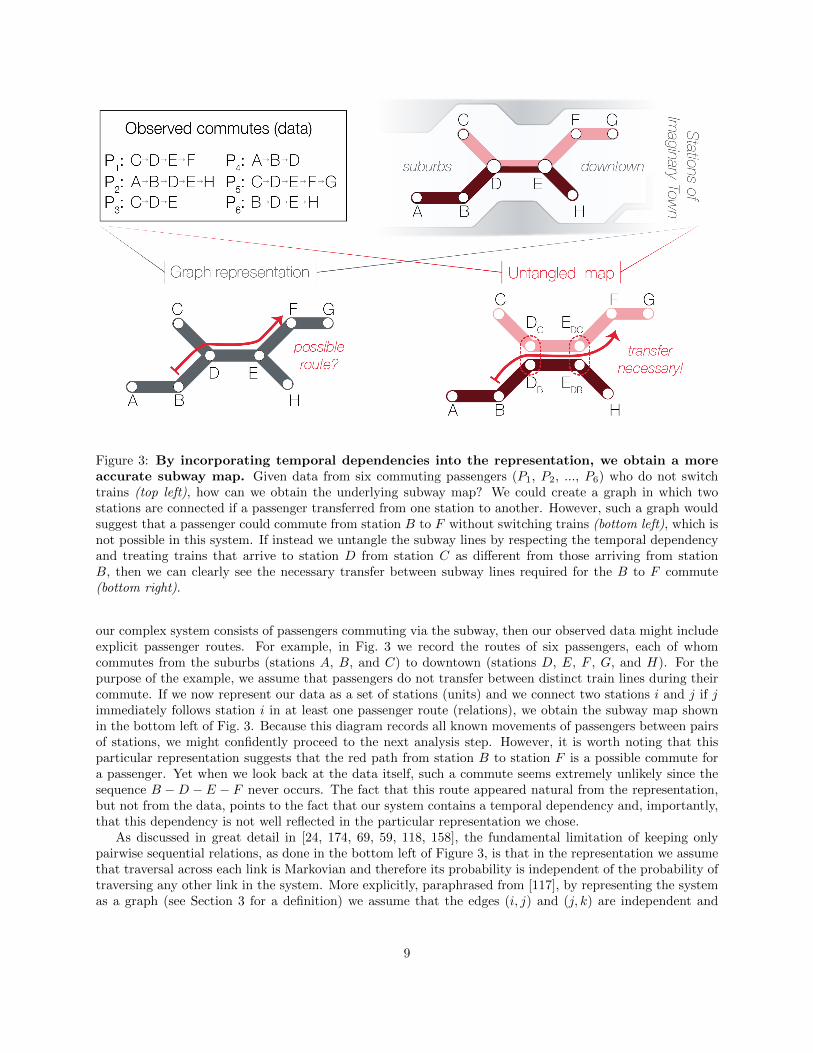
Figure 3: By incorporating temporal dependencies into the representation, we obtain a moreaccurate subway map. Given data from six commuting passengers (P1, P2, ..., P6) who do not switchtrains (top left), how can we obtain the underlying subway map? We could create a graph in which twostations are connected if a passenger transferred from one station to another. However, such a graph wouldsuggest that a passenger could commute from station B to F without switching trains (bottom left), which isnot possible in this system. If instead we untangle the subway lines by respecting the temporal dependencyand treating trains that arrive to station D from station C as different from those arriving from stationB, then we can clearly see the necessary transfer between subway lines required for the B to F commute(bottom right).

our complex system consists of passengers commuting via the subway, then our observed data might includeexplicit passenger routes. For example, in Fig. 3 we record the routes of six passengers, each of whomcommutes from the suburbs (stations A, B, and C) to downtown (stations D, E, F , G, and H). For thepurpose of the example, we assume that passengers do not transfer between distinct train lines during theircommute. If we now represent our data as a set of stations (units) and we connect two stations i and j if jimmediately follows station i in at least one passenger route (relations), we obtain the subway map shownin the bottom left of Fig. 3. Because this diagram records all known movements of passengers between pairsof stations, we might confidently proceed to the next analysis step. However, it is worth noting that thisparticular representation suggests that the red path from station B to station F is a possible commute fora passenger. Yet when we look back at the data itself, such a commute seems extremely unlikely since thesequence B −D − E − F never occurs. The fact that this route appeared natural from the representation,but not from the data, points to the fact that our system contains a temporal dependency and, importantly,that this dependency is not well reflected in the particular representation we chose.

As discussed in great detail in [24, 174, 69, 59, 118, 158], the fundamental limitation of keeping onlypairwise sequential relations, as done in the bottom left of Figure 3, is that in the representation we assumethat traversal across each link is Markovian and therefore its probability is independent of the probability oftraversing any other link in the system. More explicitly, paraphrased from [117], by representing the systemas a graph (see Section 3 for a definition) we assume that the edges (i, j) and (j, k) are independent and

9

Figure 4: Spatial dependencies within a system can complicate our representations of the data.In our example system, we have (Left) connection information that is independent of any system embedding,and (Middle) spatial information indicating where the nodes physically reside. A possible combination ofthe two information types (Right) can be used to better understand the physical constraints on the topology.If long distance connections are costly for that system, the combined representation allows the investigatorto assess the prevalence and location of those costly (and thus potentially surprising) connections.

that the two-step transition from i to k proceeds in two independent steps. This assumption can easily beviolated by a real system, as seen in our toy example, since sometimes one step in this traversal is dependenton which steps came before (i.e. transitions are not Markovian). Mismanaging temporal dependencies insystems can lead to misleading results that can, for example, over-represent the importance of edges rarelyused or create non-existent connections. We will discuss a formalism that is particularly appropriate forrepresenting temporal dependencies in Section 3.

2.3 Spatial dependencies

The third and final type of dependency that we discuss here arises from the physical nearness of units withina system. For example, in the human connectome a brain region is likely to extend white matter tracts toneighboring regions, providing physical conduits for electrical activity [200]. In granular materials, resistanceto external forces relies on interactions between only particles that physically touch [156]. More generally,many spatial systems are so named because the spatial location of nodes affects their likelihood of interactingwith one another [13, 14]. Here we say that a system exhibits a spatial dependency if the distance between twoor more nodes influences the existence of a relation that contains them. More formally, consider a systemwhose nodes are labeled by V = v1, v2, . . . , vn and each node vi has associated to it a point xi in somemetric space. Then, this system exhibits a spatial dependency if the probability of a relation between nodesv1, v2, . . . , vk is a function of the pairwise distances between the corresponding locations x1, x2, . . . , xk.

Many such systems exist in the natural and manufactured world. Indeed, spatial restrictions influencecommunication in cell populations [116, 165], trade in economic networks [98], and passengers in transporta-tion networks [221, 122]. As an example of spatial dependency within an abstract system, we might beginwith only knowledge of the pattern of related nodes. We display this structural information in the left panelof Fig. 4 with circles corresponding to nodes and lines joining circle pairs whose corresponding nodes arerelated. From the structural information alone we might expect that relating the pink and red nodes is justas difficult or costly as relating the red and dark red nodes; we might therefore infer that the two relationsare equally crucial to the system’s function. However, if the system exists within an environment containingcoordinates and a distance function, with each node having spatial coordinates and a measure of distancebetween each pair, then this spatial information could offer a different perspective on the system. In themiddle panel of Fig. 4, we see that the nodes, now depicted with colored pins, are spread out so that someare more spatially clustered whereas others are less so. Considered alone, the spatial information gives usno insight into the actual relations present in the system, but does provide information with which we might

10

predict the likelihood that nodes are related.In many spatial systems such as the brain or city transportation, relations between distant nodes are

unfavorable due to a higher cost of creation and maintenance, while short-range relations are far easier toconstruct. In the face of this association between the physical distance across a relation and its cost, we mightconsider the distances between nodes and infer that the red and dark red nodes are likely to be related, whilethe pink and red nodes are not. When we finally combine the topological and spatial information (Fig. 4,right), we then can leverage the two information types to understand which relations are most surprising ormake hypotheses about which relations are most important to the system. For example, the dyadic relationbetween the pink and red nodes might be very costly given the long distance, so we might infer that thepink to red relation is more essential to the system than the red to dark red relation since the system wouldonly spend valuable resources to maintain such a relation if it was integral to system function. Withoutthe spatial information, we may have incorrectly placed the same importance on the pink-to-red and thered-to-dark red relations. This example highlights one of many ways in which we could integrate spatial andstructural information.

As with the previous dependency types, failure to account for a spatial dependency can greatly bias ourmodels and results. Consider an outbreak of a contagious disease. If we recorded the habits of infectedindividuals such as their diet, but fail to record their locations and physical mobility through space [208, 7],then we might – for example – wrongly attribute disease spread to the broad consumption of a particular foodthat is prevalent in the infected region instead of through person-to-person contact. As another example,social contacts are also influenced by proximity. If we return to evaluating Marta’s popularity, the observationthat she has many friends may come from the fact that she lives in a densely populated area, rather thanfrom her charisma or personality. In these examples, failing to account for spatial dependencies may resultin attributing certain structural properties of the system to the wrong cause.

2.4 External sources of dependencies

Before we shift our focus to concrete ways of encoding system dependencies using mathematical formalisms(Section 3), it is useful and interesting to consider how external forces can influence the observed systemdependencies. Ideally, we as investigators would have the ability to measure all dependencies within thesystem under study, and then use this knowledge to make an informed decision as to the appropriateformalism with which to model our system. However, often the processes of scientific inquiry do not proceedso effortlessly: no analysis is ever devoid of the influence of external factors, or biases. Our goal in thissection is to highlight possible sources of such bias. Although we have already discussed biases arising fromdependencies native to the system under study, here we emphasize that acknowledging and understandingdependencies imposed by outside sources should also play a crucial role in determining an appropriaterepresentation and subsequent analyses.

• Data availability. One notable and common constraint in science is the limited data that can beempirically acquired from a given system. In other words, researchers usually have access only to afragment of the system. As a consequence, any dependency that is observed and ultimately encodedmay be determined more by the sparsity of available data than by the system’s true structure andfunction. For example, one may have access to only sparse snapshots of or short sequences froman evolving system [188], making the subset dependency difficult to identify and effectively encode.Particularly, there may not be enough data available to correctly deduce the predicates P that a subsetmust satisfy in order to also form a relation (see the definition of subset dependency in Section 2.1).

• Data acquisition or processing. Certain experimental techniques or computational proceduresmay produce spurious dependencies. A common example involves correlation matrices. By computingthe correlations of node activity (a common approach in fMRI-based functional connectivity matrices[211, 88]) one induces a transitivity dependency, which is a type of subset dependency. Concretely, ifA,B,C are nodes in a system where two nodes are related if the time series of their activities are highlycorrelated to each other, as determined by some data acquisition method, then whenever A and B are

11

Figure 5: Understanding system dependencies is a first step in the complex system analysispipeline. Types of dependencies include spatial, temporal, and subset dependencies. Acknowledging de-pendencies at this step allows for proper preservation of dependencies throughout the rest of the analysispipeline. When preserving all dependencies is not possible due to factors outside the control of the researcher,acknowledging this inability frames the results in a proper context.

related, and B and C are related, it is highly likely that A and C are also related. In this case, it ispossible that relations between nodes implied by the calculated correlations are found in the processeddata but not in the system itself. For example, one might find that changing the type of correlationresults in a change in the inferred relations.

• Research question. The research question at hand will influence which relations within a systemare particularly interesting. Moreover, it may also influence the very definition of a relation. Forexample, consider a system of proteins that interact to form protein complexes. If we wish to studywhich proteins appear together in many complexes, then we may define a relation as k proteins thatparticipate in the same complex. If instead we wish to study protein complexes themselves, we coulddefine a relation as a set of k proteins that all together form a single complex. In the first case, therelations are tied to a subset dependency (if three proteins appear together in a complex, then so doany two of them), but the second does not. On the flip side, a given research question may neglect arelevant dependency in the system. For example, we could ask if a common food could have caused adisease outbreak. Answering that explicit question neglects the fact that individuals near each otherwill likely eat similar foods. The research question is not broad enough to incorporate the spatialinformation as part of the answer, and therefore spatial dependencies may seem irrelevant at firstsight, when they may be in fact essential to finding the real answer. We expand upon this topic inSection 3.5.

To summarize, we have defined and discussed three types of dependencies that could exist in a complexsystem: subset, temporal, and spatial. We emphasize that dependencies can arise from within the systemitself or from external factors, but regardless of their origin, we as researchers must be aware of their existenceand how they influence our models and results, especially given their early position in our analysis pipeline(Fig. 5). As we will continue to see in the sections that follow, the recognition and encoding of dependenciescan greatly affect the results of our analyses and the conclusions that can be drawn.

12

3 Formal representations of complex systems

Over the years many representations of complex systems coming from different mathematical and computa-tional formalisms have taken hold across scientific disciplines. Different formalisms allow for the modelingof unique aspects and dependencies of each system, but the multiplicity of available formalisms presentschallenges for the communication, collaboration, and ultimately the progress of complexity science. Further-more, the choice of formalism also complicates the analysis pipeline that researchers must decide upon whenstudying a particular system.

Here we discuss three of the many possible mathematical formalisms that researchers commonly useto represent their system: graphs, simplicial complexes, and hypergraphs, chosen for their prevalence inthe complex systems literature. A complex system is, at its core, a collection of units and their relations,therefore we require our representations to mirror this composition of units and relations. The units ofall three formalisms discussed here are called nodes. Graphs represent pairwise relations among nodes asedges. Despite their simplicity (or perhaps because of it), graph representations have supported severalimportant discoveries such as the prevalence of small-worldness in real-world networks [220, 6]. Still, graphscan only, by nature, represent dyadic relations between nodes2. If instead relations within the system existbetween more than two nodes, one might turn to either a simplicial complex or a hypergraph. Both ofthese formalisms naturally allow us to encode such polyadic relations [21]. The relations represented by asimplicial complex are called simplices and those represented by a hypergraph are called hyperedges. Wewill first define each formalism, so that later in this exposition we can explicitly discuss their respectiveadvantages and assumptions.

3.1 Graphs

The first and perhaps most common formalism used to model complex systems stems from graph theory.A graph G is a collection of nodes and edges between nodes such that an edge connects at most two nodes(Fig. 6, left). We denote the set of nodes as V and the set of edges E ⊆ V × V , so that a graph is defineduniquely by G = (V,E); note that each edge is an unordered set of two nodes. The nodes of a graph are theunits, and edges describe how these units are related. If vA and vB are nodes of the graph, then we write(vA, vB), or vA − vB to represent the fact that the two nodes are connected by an edge. Studies that form agraph representation from the underlying data frequently involve finding densely connected sets of nodes ordetermining how an object might traverse the structure. In using the graph representation, such questionscould lead to detecting cliques or communities in the graph, or identifying chains of connected nodes calledpaths (see Fig. 6, left, and Section 5.1 for more examples).

Many attribute the origin of graph theory to Leonhard Euler in the 18th century [74]. One can also traceits presence outside of mathematics back to the use of sociograms and social network analysis in the 1930s[78], and to graph-like data structures in computer science in the 1950s [222]. Notably, the use of graphsto model more general complex systems has rapidly increased over the past few decades, driven largely bythe discovery of the small-world effect [220] and heavy-tail degree distributions [10] in real-world datasets.Encoding a system as a graph has the great advantage of hundreds of years of mathematical theory behindconcepts, generally simple computations, and insightful visualization. However, the graph by definitionassumes that relations between nodes occur exclusively at the pairwise level. Systems such as transportationnetworks might solely contain pairwise relations among their units, but many others, especially from biology,often have polyadic relations. Still, the graph’s ability to model systems has proven quite useful in distinctfields such as neuroscience [17, 36], computer science [75, 132], and ecology [161, 135].

2More precisely, edges in a graph can only involve (at most) two different nodes. Whether the interpretation of each ofthose nodes is that of a single unit or many units (as is done for example in some representations that involve the idea of a“supernode”), is not a relevant matter for graph theory, but for the process of encoding data into a graph.

13

Figure 6: Three types of formalisms composed from nodes and relations. (Left) Graphs involve unitscalled nodes and relations between two nodes called edges. Possible features of interest for graphs includeall-to-all connected sets of nodes called cliques, as well as routes between nodes called paths. (Middle)Simplicial complexes can be used to represent systems with polyadic relations among units. Sets of relatednodes are connected by simplices. A k-simplex describes k + 1 nodes that collectively interact, such thatany subset of nodes forming a simplex must also form a simplex; this is called “downward inclusion”. Motifsof interest include topological cavities and maximal simplices. (Right) Hypergraphs can also be used torepresent systems with polyadic relations among units. Sets of related nodes are connected by hyperedges.Hypergraphs are not restricted by downward inclusion. Of particular interest within a hypergraph is theabsence of a substructure (or smaller relation), for example in which two nodes do not connect dyadicallybut participate together in a hyperedge that connects a superset of the node pair.

14

3.2 Simplicial Complexes

The next formalism that we consider addresses the need to acknowledge polyadic relations in the system.Illustrated in the middle column of Fig. 6, a simplicial complex is a set of nodes V (also called verticesin the field) along with a collection of subsets of nodes R (often denoted by K in the field) such that forany r ∈ R and r′ ⊂ r, we have r′ ∈ R; we will refer to this condition as “downward closure”. A set ofk + 1 nodes r ∈ R is called a k-simplex, and downward closure requires that any subset of nodes within asimplex also forms a simplex. In practice we often imagine a k-simplex to indicate an application-relevantinteraction between the k + 1 nodes, such that these nodes may function in unison. The simplicial complex(precisely, the abstract simplicial complex ) would then record the individual units (nodes), the functionalbuilding blocks (simplices), and how all these building blocks are assembled into one system (the simplicialcomplex). Since subsets of simplices are simplices by definition, then if k nodes are related, we have thatany subset of those k nodes are also related. The simplicial complex can be written as a binary incidencematrix of dimensions #maximal simplices × #vertices where an element containing a 1 indicates nodeparticipation in the corresponding maximal simplex; a maximal simplex is a simplex that is not containedin any larger simplex.

Although algebraic topology has been studied for well over a century, it was not until the late 1990’s thatapplied algebraic topology as a discipline began to emerge [230, 68] (though we note a earlier uses exist [9]).Many of the earliest studies used applied topology and simplicial complexes to study data in the form ofpoint clouds [40, 189]. Later, it became clear that the simplicial complex language was a natural formalismfor explicitly representing biological and physical systems. For example, simplicial complexes have been usedto represent neural recordings [86, 53], classify images [203, 55, 66], and describe the mesoscale architectureof brain networks [201, 202, 167, 191, 159]. Even more recent work has focused on defining generative modelsto construct simplicial complexes with given topological features [51].

3.3 Hypergraphs

The final formalism that we consider draws again from sets of nodes and their relations, yet is even moregeneral than the simplicial complex discussed above. The hypergraph is an extension of the mathematicaldefinition of a graph, in which we have a node set V and a hyperedge set R (sometimes denoted in thefield as E ). A hyperedge e ∈ R can connect an arbitrary number of nodes. That is, while an edge in agraph can only connect two nodes, a hyperedge can connect three, four, five, or more nodes (Fig. 6, right).More rigorously, a hypergraph is a pair (V,R) with V a node set and R a set of subsets of V [214, 26].In contrast to the simplicial complex, we can use the hypergraph to encode polyadic relations without therestriction of downward inclusion. Formally, a subset e′ of a hyperedge e, e′ ⊂ e ∈ R, does not necessarilyexist as a hyperedge. Additionally, we can rewrite a hypergraph as a binary incidence matrix of dimensions#hyperedges×#vertices in which an entry of 1 indicates the node participation in the hyperedge.

As noted above, the crucial restriction that is relaxed when moving from a simplicial complex to ahypergraph is that of downward closure. Recall that in a simplicial complex any subset r′ ⊆ r of a simplex rmust also be a simplex. Hypergraphs do not obey this rule. For example we may see a hyperedge connectingvertices v1, v2, and v3 but no hyperedge that connects v1 to v2 exclusively. Or, given two hyperedgesconnecting nodes v1, v2, v3, and v2, v3, v4, if a hyperedge connecting v2, v3 also existed, does this smallerhyperedge indicate a sub-relation for the hyperedge v1, v2, v3, the hyperedge between v2, v3, v4, neither, orboth? With a hypergraph, we cannot determine how or if a sub-relation emerges due to superset relations(see [195] for a deeper discussion). This subtle difference allows hypergraphs to represent a wide diversityof systems, including many that the simplicial complex formalism would not appropriately represent. Thehypergraph’s increase in modeling flexibility is counterbalanced by a decrease in formal analysis methods,which we will discuss more in Section 5.

The flexibility and ability to model polyadic relations made hypergraphs an appealing formalism inmany systems that were originally studied with graph theory. Indeed one of the earliest practical uses ofhypergraphs was to understand social networks [184]. Since then, researchers have successfully employedhypergraphs to study polyadic relations in the Enron email dataset [162], find the core of yeast protein-protein

15

interactions [163], uncover motifs in neurodevelopment [89], track changes in evolving systems [18, 56, 57],and detect failure in biochemical networks [110]. As many uses of hypergraphs arose out of systems firstmodeled with graphs, many analysis methods for hypergraphs mimic those originally used for graphs (wediscuss this point further in Section 5.3).

3.4 Variations

We note that the above descriptions only scratch the surface of complex system encoding possibilities. Anever broadening set of scientific questions drives the need for novel variations of each formalism, resultingin a myriad of definitions and manipulable parameters. One could extend our mathematical definition ofcomplex systems to include the following properties, as a map p : V ×R→P where P is a set of propertieswe care about, as mentioned in Section 1.1. Here we note a few of the most common modifications to eachof the above formalisms, driven by the need to incorporate more information about the system at hand.

Directed

Many complex systems including the brain, transportation networks, and metabolic pathways exhibit direc-tionality in their relations. That is, in these systems, if vA and vB are units that share a dyadic relation,there is a meaningful distinction between a relation where vA comes first, one where vB comes first, andone where either vA or vB comes first (but there must always be an order in how they are related). Todistinguish these cases we write vA → vB , vB → vA, or vA ↔ vB , respectively. If we apply this idea tothe graph formalism, a directed graph is one where each edge is now an ordered set of two nodes. Directedgraphs have proven extremely useful in many contexts from scheduling and monitoring workflows [112, 1]to cardiac excitation modeling [212] to understanding percolation processes relevant to wild fires and otherexplosive phenomena [197, 65]. Moving to simplicial complexes, directionality is still quite natural. Indeedsimplices themselves inherit a directionality, formally known as an orientation, encoded by the numberingof the participating vertices. In practice, in an oriented k-simplex, each node is made to point only tonodes with a higher assigned number. Oriented simplicial complexes arise in practice from directed synapsesbetween neurons [167] as well as directed migration flow [100]. Finally, in hypergraphs, one may representdirectionality with hyperarcs, the term for a directed hyperedge. More formally, a hyperarc is a pair ofdisjoint subsets of vertices with one subset comprising the sources and the other subset comprising the sinks[82]. Directed hypergraphs have proven useful in constructing a biological pathway database [113], tacklingproblems in computer science such as propositional logic [82] and combinatorial optimization [119, 87], andfinding specific patterns of connectivity in chemical reaction systems [149], among others.

Weighted

In real-world systems, not all relations are created equal; even within the same system, relations betweenindividual units may vary in strength or magnitude. To represent these differences, the strength of a relationcan be encoded using the weighted versions of the above formalisms. To assign weights to any of the aboveencodings, we can define a general weight function W : R → R from the set of relations R (edges, simplices,or hyperedges) to the real numbers R. For a graph, this function would assign a value to each edge, whichwe generally interpret as the strength or frequency of the pairwise interactions between the correspondingnodes. In the context of weighted representations, the original versions containing no weights are calledbinary or unweighted, as they can be cast as weighted objects where the weights of all relations are eitherone, if they exist, or zero if they do not exist. The brain connectome, traffic between municipalities [62],and functional similarity of genes [153] have all been modeled as weighted graphs. Additionally, manycommon graph metrics such as the clustering coefficient and path length (covered in more detail in the nextsection), extend easily to the case of weighted graphs [175], making this variant of representation particularlypervasive. Similarly we can construct a weighted simplicial complex by assigning a weight to each simplex.However, recall that in a simplicial complex any face of a simplex must also be a simplex, and thus if wehave a relation between k nodes then any subset of these nodes must be related to at least the same extent

16

as the superset. Said another way, we require that the weighting function W on simplices adheres to the rulethat for any simplex r, if r′ ⊆ r then W (r) ≤ W (r′). Weighted simplicial complexes can arise from pointclouds with inverse distances between points as weights or from growing processes with time of additionused to assign simplex weight. Perhaps most often, we study weighted simplicial complexes through the lensof persistent homology, which computes the organization of topological cavities housed within the weightedsimplicial complex [230, 39, 83, 148] (see a few recent uses in [191, 86, 159, 201]). Lastly, in hypergraphswe can naturally weight hyperedges with distinct values [82]. Importantly, weighting hyperedges allowsmore flexibility in choosing weights, as weighted hypergraphs do not enforce rules restricting weights onsubedges in contrast to weighted simplicial complexes. Weighted hypergraphs have proven useful in imagesegmentation [169] and in the process of incorporating prior knowledge into learning algorithms [207].

Dynamic

Complex systems such as cell signaling, traffic patterns, and transactional relations also grow, separate,or fluctuate in time [124, 176, 44, 121]. Consequently, formalisms have been adapted to represent such anevolving architecture. A dynamic graph or a temporal graph is a sequence of graphs G1, . . . , GT in which eachGi is a graph on the same set of nodes, and each node is mapped to its identity when moving from Gi to Gi+1

[95]. As with other variations on graphs, multiple computational tools such as community detection havebeen extended to include these types of dynamics [143, 190, 138]. Moving to simplicial complexes, a dynamicsimplicial complex is similarly a sequence of simplicial complexes on the same node set. Questions about thetopological cavities of simplicial complexes can be answered by using vineyards [224] and zig-zag persistenthomology [131] depending on the types of evolving simplicial complexes. Finally, a dynamic hypergraphis a sequence of hypergraphs H1, . . . ,HT on the same node set where hyperedges may change from Hi toHi+1. At the time of writing, we found few examples of applied dynamic hypergraphs, although we notethat their visualizations have been studied [210]. Nevertheless, we suggest that this particular variation ofhypergraphs could be useful for example in modeling evolving gene interactions, functional relations betweenbrain regions, and the time-varying structure of social groups.

Multilayer

Often the units or relations of a system have types, categories, or classifications that distinguish them. It issometimes useful to distinguish between these types of relations in our representations, and one way to do sois to use the so-called multilayer variations. Generally, multilayer graphs consist of a set of graphs that may(or may not) involve the same nodes; each graph in the set comprises a layer. The graph in a given layercontains relations of exactly one type. Consider a human brain in which two regions might show an increasein blood flow either due to coupled neuronal activity or due to interactions involving nearby blood vesselsthemselves. To encode these two types of relations in a single representation, we could use a multilayer graphwith two layers: one encoding the relations between neurons and another encoding relations between bloodvessels. We note that when all layers contain the same set of nodes and the only interlayer edges that existconnect nodes to themselves in other layers, the representation is called a multiplex graph [31, 193]. Weinvite the interested reader to visit [108, 29] for more rigorous definitions, and [129, 35, 226] for implicationsfor diffusion and control. Time-evolving systems can be seen as a subtype of multilayer systems, in whichthe layers are a set of graphs ordered in time. Previous studies have used multilayer networks to modelcomplex spreading processes [58, 178, 179, 209], understand explosive word learning [198], and uncover thecommunity structure of trade relations [11]. Multilayer simplicial complexes or hypergraphs would similarlyinclude a set of simplicial complexes (respectively, hypergraphs) not necessarily defined on the same nodesin each layer. As of the time of this writing, we did not find applications yet of this extension. We suggestthat these variations could prove useful for understanding multiple types of biological data collected on a setof nodes. As an example, one could encode common properties (mutation status, chromatin rearrangements,etc.) as layers in a multiplex network of cancer cell lines in order to better understand drug response [166].The multilayer variation is readily applicable whenever researchers have access to and want to model twodifferent fragments of the same system.

17

Higher Order Networks

Higher Order Networks (HONs) are a variation of the graph formalism that aims to represent a certain kind oftemporal polyadic relations. Instead of encoding system units as nodes, the HON encodes frequent paths ortransitions in the data as nodes, which then allows us to interpret the final representation with the standardMarkovian assumptions on edge sequences. Recall our example of commuting passengers in Figure 3. Wecan build a HON from the observed path data to encode the observed dynamics and temporal dependenciesof this system in a particular kind of graph. In Figure 3, the more accurate subway map on the bottom right,reconstructed from the observed data, contains two nodes that correspond to the physical station D. The onelabeled DB represents the passengers that arrive to D from station B, while DC corresponds to those thatarrive from station C. Similarly, the physical station E splits into two nodes: EDC and EDB . The nodes onthis map do not correspond to the stations observed in the town’s transportation system, but to the possiblepassenger pathways through them. Indeed, as observed before, we never observe a passenger commute thattraces the path C −D−E−H: all passengers that pass through stations C −D−E, in that order, then goon to station F , while all passengers that pass through stations B−D−E, in that order, go on to station H.Therefore, the representation on the bottom right of Fig. 3, an example of a higher-order network or HON, isa more faithful representation of the observed data and its temporal dependency. Note that if the observedpassenger data changed to include a route visiting stations C −D−E−H, the structure of the HON wouldchange, even if the physical brick-and-mortar subway system, and its graph representation, would not. Wediscuss HONs in the next subsection and refer the interested reader to [24, 174, 69, 59, 118, 158] for furtherdetails.

Further variations

We note the above variations on the three main formalisms discussed are only the beginnings of possible waysto extend these representations. Depending on the complex system and questions at hand, certainly onemay combine the variations described above to make, for example, an edge-weighted dynamic network [106],a weighted multilayer network [130], a multi-order network that combines multiple HONs [182], or anothercombination that provides an effective representation. One may also study systems of weighted nodes insteadof weighted edges [192, 140], as well as representations where each node has some kind of internal structure[48, 71] or possible action [8] . Any of the formalisms above could also lend itself to studying the intricacies ofcoupled dynamical systems such as coupled oscillators [155, 147] or interacting threshold-linear models [136].Indeed when including variations on the three formalisms covered in this review, we find we can encode animpressive range of complex system types and properties.

Other Formalisms

We recognize that many other formalisms intended for complex systems exist and that those we specificallymention in this review constitute only a small subset of the possibilities. Other possible formalisms includegraphons, which describe limits of sequences of graphs and can be used to estimate large, noisy systems[33], metapopulation models which classically describe global behavior of many local species populations[120, 204, 93] and can be adapted to networks [48], random sequences of sets [25], and sheaves which canhandle added information on each node in a network and have previously been used to frame the networkcoding problem [84] and find consensus in sensor networks [52].

3.5 Encoding system dependencies

As we discuss above, the formalism used to encode our data should be carefully chosen to respect anyprominent properties of the system, and specifically the dependencies found therein. In this subsectionwe discuss the subtleties of choosing an appropriate formalism, and then review the common practicesthat researchers use to encode subset, spatial, and temporal dependencies using the formalisms we haveintroduced.

18

Once we have chosen which dependencies to model, it is important to carefully determine when twoor more units in our system are related to each another – i.e. to define the relations in our model (Fig.7.) Depending on the exact definition of the relations, the resulting representation may or may not exhibitthe desired properties, or it may even exhibit properties not found in the actual system, but coming fromexternalities from the data, as discussed in Section 2.4.

For example, consider recording brain activity from an individual as they progress through differenttasks (reading, watching a video, resting, etc.). Different tasks require the activation of distinct sets ofbrain regions. How do we define relations between brain regions? As depicted in Fig. 7, we could definek nodes to be related if a task requires all k nodes to be active. Alternatively, we could define a relationbetween k nodes if the k nodes were found to co-activate during a task. Finally we could call two nodesrelated if they have a high enough measure of pairwise similarity, perhaps assessed by correlation or mutualinformation. Depending on our chosen definition of node relations, our resulting representation either will orwill not encode a subset dependency. In this example, only the definition of node co-firing exhibits a subsetdependency, which we could capture in a simplicial complex representation. Now consider a city bus systemfragment including stations, roads, and bus lines (Fig. 7, bottom). First, we could define a relation betweenk nodes (stations) as the sets of stations along an entire bus route. That is, k stations are related if theytogether form a whole bus route. This definition would propagate no subset or temporal dependencies to therepresentation. Second, we could instead call k nodes related if they share at least one bus line. Consequentlywe now have a subset dependency that must be captured by our choice of representation. Third, we mightdefine two bus stations as related if they are subsequent stops along a route. This third, inherently pairwise,definition of relation could be represented with a graph. Note that none of these three definitions encodethe temporal dependency, which may or may not be present in the available data. For example, if we hadaccess to, not only stations’ locations, but also passenger trajectories within the system, we could encodethe temporal dependencies using HONs.

The above examples, and those in reference [195], illustrate the fact that one must carefully chooserelations to effectively encode dependencies, or, equivalently, that whether or not a given representationexhibits a dependency is a (sometimes subtle) question of semantics. This is to say, the modeling choicesconcerning relations, representations, and dependencies are highly, and unavoidably, interdependent on oneanother. We must be aware of what dependencies exist in the system, which of those are encoded orneglected in the representation, and which come from external sources. In the scientific community, thesedifficult choices are usually made following the common practices that we delineate next.

Encoding subset dependencies

If a system exhibits subset dependency, it is common practice to use either simplicial complexes or hy-pergraphs to represent it. In the case when any subset of a set of related units are also related, then anappropriate formalism is the simplicial complex, since this formalism has the downward inclusion property(see Section 2.1). In the terms used in Section 2.1, the predicate P is true for any subset of an existingrelation. If instead only some subsets of related units are related, then one could argue that a hypergraphis the appropriate formalism to use, since it allows for great freedom in encoding relations among subsetsof related units. Equivalently, a particular subset dependency gives a particular choice of the predicate P ,which in turn induces a particular hypergraph. Recall that the important difference between hypergraphsand simplicial complexes is the notion of a subedge. Drawing from Remark 3.5 of [195], if a 1-simplex {a, b}and two 2-simplices {a, b, c} and {a, b, d} exist, then by definition {a, b} is a sub-relation (formally called aface) of both {a, b, c} and {a, b, d}. However, if instead we had hyperedges {a, b}, {a, b, c}, and {a, b, d} in ahypergraph, we cannot say if {a, b} is a sub-relation (sub-edge) of {a, b, c}, {a, b, d}, both, or neither. Thisconnection or lack thereof between relations and sub-relations crucially affects interpretation of the systemrepresentation.

19

Figure 7: Native dependencies captured by the definition of relation. (Top) We might recordthe on/off activity of four brain regions in each of four tasks (left). Depending on the definition of relationchosen (middle), we may or may not record a dependency in a representation (right). (Bottom) Given five busstations placed along a set of roads (dashed lines), we observe three bus lines that connect the stations (left).Depending on the definition of relation chosen (middle) we might include a subset or temporal dependency,which we would want to capture in our representation of the system (right).

20

Figure 8: Choosing a formalism marks the second step of our analysis pipeline. Formalisms includegraphs, simplicial complexes, and hypergraphs. We argue that the choice of formalism should be made inorder to most faithfully capture system dependencies.

Encoding temporal dependencies

As discussed in Section 3.4, one way to encode temporal dependencies uses the idea of Higher Order Networks(HONs). Recalling our previous description, the HON begins with a set of walks, and from the patternsfound therein creates a graph in which nodes correspond to ordered sets of units in the original system, andedges connect nodes based on temporal dependence. In this way, the HON takes the temporal dependency(for example, paths from A to B always lead to C), and encodes it in a special kind of node, derived fromthe original units of the system. At the time of writing, HONs have been defined for paths on graphs.It is still an open question how to extend the HON formalism to simplicial complexes or hypergraphs sothat the resulting representation could exhibit both temporal dependencies and arbitrary subset (or spatial)dependencies.

Encoding spatial dependencies

Possibly the most straight-forward method to encode spatial dependencies constructs a weighted graph inwhich the edge weights in some way represent how close or far nodes lie from each other. However, wehighlight the fact that edge weights are a popular mechanism to encode other kinds of information as well,and once we encode one piece of information within the edge weight we cannot then use edge weights to alsoencode spatial dependencies. For example, if we build a graph for the transportation system of a city, wemay want to encode both traffic flow and road length as properties of the relations. Usually, both types ofinformation are encoded using edge weights, so we are left with three alternatives. The first is to choose anedge weight that aggregates both types of information. The second is to use a multilayer network (see 3.4)in which each layer has weighted edges reflecting a single type of relation [44]. The third is to create a moreholistic representation that efficiently combines the spatial information, traffic flow, and road length whilealso including any interactions between edge types. This challenge is yet another example highlighting thatdata availability, system dependencies, and choice of representation are not independent of one another.

If the only challenge to the study of complex systems were the choice of representation, then our discussionwould be near complete. However, real-world systems usually have at least two or more dependencies,including those we do not discuss in this paper. For example, the subway network (Fig. 2.2) contains bothtemporal dependencies (evidenced in passengers’ routes) and spatial dependencies (the routes taken areusually constrained by geographical proximity); while the co-author system (discussed further in Section 6)

21

could be further constrained by both temporal and subset dependencies. Moving forward (Fig. 8), we willneed to develop novel methods for systematically representing and encoding complex systems with multipledependencies.

4 Mathematical relationships between formalisms

At this point it may seem that the choice of representation wholly restricts the perspective and possible anal-yses on the data. For example if we encode the data as a directed hypergraph, we can only perform analysesusing hypergraph methods. However as each of these base formalisms record relations between nodes, per-haps we could utilize the underlying mathematical relationships between each of these formalisms to gainadditional insights. In this section we will explore the formal mathematical relationships between graphs,simplicial complexes, and hypergraphs, and then we will discuss the assumptions needed or information lostas we move from one to another.

From hypergraph to simplicial complex: Forgetting independent relations

First let us imagine that from our data we have constructed a hypergraph H. If we would like to createa simplicial complex KH from H, we might first map the nodes of H to nodes of KH , before dealing withthe hyperedges. Recall that in a simplicial complex we have simplices that connect multiple nodes, butwe also have the downward closure restriction that if we have a simplex r, then any r′ ⊆ r must also bea simplex. So then to form KH we could take any hyperedge connecting k + 1 nodes and form from it ak-simplex (Fig. 9 top left), thereby forcing the downward closure of the hyperedge relation so that the systemrepresentation can abide by simplicial complex rules. Additionally note that if we have a hyperedge a onnodes {v0, . . . , vk} as well as a hyperedge b on a subset of these nodes, the simplicial complex will view b asredundant information, since by definition every subset of nodes in a will be connected by simplices. In thisway, we say that the simplicial complex “forgets” the existence of b as a relation observed independently ofall other relations (specifically, observed independently from the relation a). We can also see this forgettingnotion in the matrix representation of the structure itself: from a hyperedge incidence matrix we onlyneed to keep the maximal hyperedge rows in order to build the corresponding simplicial complex incidencematrix. Additionally, KH will also lose information regarding the total number of relations in which a nodeis involved, since many of those original hyperedge relations may be a subset of another hyperedge relation.On the other hand, this procedure allows us to access methods that are available for simplicial complexesbut not for hypergraphs (discussed more in Section 5). Overall, in the hypergraph each hyperedge between aset of nodes arises independently, so that having additional hyperedges (or the lack thereof) between subsetsof nodes within a larger hyperedge indeed supplies more information than the one largest hyperedge. Incontrast, we can define a simplicial complex by its largest simplices (formally called maximal simplices)alone.

From simplicial complex to graph: Forgetting polyadic relations

Next let us assume that we are given a simplicial complex K, and that from K we wish to construct agraph GK that still represents our data. This transition is more straightforward, as we can take all of the1-simplices of K to be edges of the graph GK . Said another way, if two nodes participate in the samek-simplex in K, then we draw an edge between these two nodes in GK (Fig. 9, top right). By performingthis transition from simplicial complex to graph, we are now forgetting polyadic relations between nodes.For example, in a simplicial complex we may have three nodes connected by three 1-simplices, or connectedby three 1-simplices and a 2-simplex; in a graph, by contrast, we can only show these three nodes as beingall-to-all connected by edges thus eliminating our ability to distinguish between the two cases. One canalso move from a hypergraph to a graph by drawing an edge between two nodes only if the two nodes wereconnected by a hyperedge. The resulting graph recovered from this process will be the same as the graphobtained by moving from a hypergraph to a simplicial complex to a graph following the described protocol.

22

Figure 9: Transitioning between formalisms requires added assumptions or engenders forgettinginformation. (Top, left) The original example system as a hypergraph. (Top, middle) When we sendhyperedges to simplices, we create a simplicial complex, and (Top, right) by keeping all edges we form agraph. Going in the other direction, we begin with the same graph (bottom right), fill in all cliques assimplices to obtain a simplicial complex (bottom middle), and send maximal simplices to hyperedges to forma hypergraph (bottom left). Note that the hypergraphs on the top left and bottom left differ from oneanother.

23

From graph to simplicial complex: Assuming polyadic relations

What happens if we instead move in the other direction? What are the assumptions necessary to take agraph such as the graph shown in Fig. 9, right, and construct from it a simplicial complex or a hypergraph?First, let us begin with a graph G and construct a simplicial complex. If we make the assumption that allnodes involved in a (k+ 1)-clique of G are related, then we can construct a simplicial complex KG by fillingin each (k + 1)-clique with a k-simplex. This particular construction is called the clique complex [104] orthe flag complex [105], and is often denoted by X(G) (Fig. 9, bottom middle). We reemphasize that forthis construction, it is necessary to assume that all nodes within a clique are all together related as a singlefunctional unit. Importantly this clique-to-simplex assumption may not be appropriate for all systems. Oneexample arises from social conversations in which three people may converse only in pairs and never togetheras a three-person group.

From simplicial complex to hypergraph: Assuming that only maximal simplices are indepen-dent

As we consider moving from simplicial complex K to hypergraph HK we are faced with a few options. First,since a simplex by definition implies that all subsets of nodes within a simplex are also related, then wecould take every simplex and form from it hyperedges between all subsets of nodes within the simplex. Inconstructing the hypergraph in this way, we carry through the downward closure restriction. Alternatively,we could perform a conversion more akin to the inverse of the hypergraph-to-simplicial-complex conversiondiscussed above by creating a hyperedge only for each maximal simplex of K (Fig. 9 bottom left). Assigninghyperedges only for maximal simplicies can be seen as a conservative approach; that is, we can uniquelydefine a simplicial complex using its maximal simplices so that in forming the new hypergraph, we areassuming the fewest number of hyperedges necessary to preserve only the polyadic relations already knownto be independent.

From hypergraph to graph, and from graph to hypergraph

Perhaps most importantly, note that from a graph we can move to a simplicial complex, then to a hypergraph,then back to a simplicial complex, and finally back to a graph following the translations discussed above. Inthis process, we will recover the original graph with which we began. However, the opposite is not the case.As depicted in Fig. 9, we can begin with the hypergraph on the top left, move through the simplicial complex,to the graph, and then move back along the bottom row from right to left and we will in fact recover a verydifferent hypergraph than the one from which we began. This exercise emphasizes the information lost orforgotten in moving down the formalism ladder. Specifically, since each hyperedge may arise independentlyof all others (most notably independently of any hyperedge that is a superset), we not only lose informationwhen moving towards a graph but also cannot recover this information when moving back up from a graphto a hypergraph.

We note that the above protocols of moving from one formalism to another do not encompass all possibil-ities. One could define a simplicial complex from a graph by simply keeping all edges as the 1-skeleton andhaving no larger simplices. Or perhaps one might form a weighted graph from a hypergraph by assigningedge weights as some function of the hypergraph structure [141, 43, 91]. Though we here discussed movingbetween formalisms as the third step in the pipeline (Fig. 10), moving from one formalism to another afterthe initial encoding of data into a formal representation should be performed only with extreme care, as anytranslation requires adding assumptions or forgetting relations or independencies.

5 Methods suitable for each representation

Now that we have exerted the effort necessary to properly represent our data as a graph, simplicial com-plex, or hypergraph, how do we analyze the resulting structure? In this section, we will describe methods

24

Figure 10: Mathematical relations between formalisms add an optional step to the pipeline, onlyto be used with caution. After an appropriate formalism has been chosen for system representation, onecan make use of mathematical similarities between formalisms to view their representation from the lens of adifferent formalism. Importantly, we note that moving from hypergraphs to simplicial complexes to graphscan result in a loss of information, while the reverse direction can require one to make assumptions aboutthe system.

Figure 11: Formalisms provide different perspectives on the neighborhood of a node. (Left) Thecolored node has four direct neighbors and participates in two triangles. (Middle) The colored node has fourdirect neighbors and participates in one 2-simplex. (Right) The colored node has two neighbors connectedto itself exclusively, and two neighbors accessible through a larger hyperedge.

and statistics that can be used to evaluate precisely how each of the three base formalisms offer uniqueperspectives on the system under study. We recognize that many such methods and statistics exist, but forclarity we will focus on a few techniques that help us identify similarities among and differences betweenrepresentations.

Before we begin, we briefly provide a note of caution. The fact that a method of interest might currentlyintake only one particular formalism does not justify the use of that formalism in representing our data.To further illustrate the point, if we intend to understand the spread of a disease by way of calculating theepidemic threshold [41], we would find that most existing methods that calculate the epidemic thresholddo so from a graph representation. The theory of disease spread on hypergraphs and simplicial complexescurrently is a nascent area of research [99, 101], so one might not find a definition of the epidemic thresholdthat uses either of these polyadic formalisms in the literature and is appropriate for the system at hand.Nevertheless, the absence of this particular notion for polyadic formalisms does not imply that we are justifiedin using a graph formalism to represent the system. Generally, a result is unlikely to offer fruitful insightinto a system if the calculation was performed on a representation that itself is ill-suited for the system.

25

Figure 12: The three formalisms and their corresponding downstream analyses can offer differentperspectives on a complex system. (Left) For this example system, a graph representation suggests aglobal core-periphery organization. (Middle) A simplicial complex representation of the same system appearsto show a globally circular structure. (Right) The hypergraph representation of the same system hints atthe presence of two communities.

5.1 Methods for graphs

As the most well-known of the three formalisms in data analysis, graphs have offered scientists interpretableand easily-computable tools for centuries. Thanks to this rich history of graph analysis, we can computa-tionally study graphs at many different levels: the local node or node-neighborhood level, a meso-scale levelto see larger patterns, and the global level to summarize the entire object. Though myriad statistics exist,for the sake of brevity we limit our discussion below and point the interested reader to [142] to learn more.

At the most basic level, the number of edges incident to a node vi is called the node degree and isdenoted ki (Fig. 11, left). The distribution of degrees can constrain the graph’s large-scale organization,for example tracking the emergence of a giant connected component [134]. At the neighborhood level, wecan investigate statistics describing the connectivity between a node’s neighbors. A common example is theclustering coefficient ci of a node vi. Formally the clustering coefficient is

ci =2µi

ki(ki − 1), (1)

where µi is the number of edges between neighbors of vi. The numerator counts the number of triangles inwhich vi participates and the denominator normalizes by the number of triangles that could possibly formaround vi. Broadly, the degree and clustering coefficient are examples of a much broader class of statisticsproposed for the description of local and neighborhood structure in graphs.

Complementing such descriptions, other statistics have been defined to measure the nature of paths in thegraph and markers of meso-scale structure. For example, the average path length, various types of centrality[79, 22], notions of modularity [90, 114, 151], and the property of small-worldness have proven useful in thestudy of a wide variety of systems from the human brain [36, 17] to granular materials [156]. One particularmethod that, at the time of writing, we found to be unique to the graph formalism, is that of core-peripherystructure. A graph with core-periphery structure contains a dense group of nodes connected to each othercalled the core, and a second group of nodes called the periphery that mostly connect to the core rather thanto other nodes in the periphery [32, 172] (Fig. 12, left). For a description of other network statistics, werefer the interested reader to prior literature [142, 175]. Additionally, we note that in real world systems, thevalues of many of these network statistics are correlated with one another over instances in a graph ensemble,and these patterns of shared variance can be used to distinguish between types of systems [50, 146].

26

5.2 Methods for simplicial complexes

Simplicial complexes entered the data analysis scene more recently than graphs. Yet, we can still use asimplicial complex to investigate multiple levels of system architecture with intuitive methods and statistics.As before, we keep this section brief by focusing only on a few basic statistics and then one method that isunique to simplicial complexes.

We might first seek to extrapolate basic graph definitions to simplicial complexes. If we view a graphas the 1-skeleton of a simplicial complex, then the graph degree of node vi corresponds to the number of1-simplices in which vi participates. By extending this idea, we can understand the neighborhood of a node(Fig. 11, middle) by defining the simplex participation of node vi as the vector P (vi) in which the kth elementis the number of (k − 1)-simplices in which vi participates. One could also record the vector of simplices inwhich the node participates (called the upper degree in [185]), or the number of simplicies not contained inany larger simplices, i.e. the maximal simplices, in which the node participates [191]. Notably, one can alsodefine the degree of a simplex of any size, instead of only defining the degree of a node (which are after all,zero-dimensional simplices) [185]. Similarly, we might ask whether and how the clustering coefficient couldbe extended to the simplicial complex formalism. Depending on the precise properties that one intendsto capture, one could use a ratio of simplices from dimensions k and (k − 1) to formalize the notion ofa clustering coefficient. However, in the simplicial complex formalism each simplex can be considered as afundamental building block, so it makes sense to also define a clustering coefficient for an arbitrary k-simplexas in [125]. In a complementary effort, the notion of centrality has recently been extended from the graphformalism to the simplicial complex formalism [73].

In addition to extending graph measures to simplicial complexes, we can also harness the theory of alge-braic topology to uncover more complicated motifs within the system. The downward closure requirementwithin the simplicial complex definition gives us the ability to accurately identify which simplices are in-volved in higher dimensional simplices. Consequently we can then detect where a dearth of simplices leavestopological voids in the complex (Fig. 12, middle). Detecting topological voids is the work of homology, andas homology relies on well-defined mappings from larger to smaller simplices, this method is best suited forthe formalism of simplicial complexes.3

Simplicial complexes can also be “reversed” in a way that can be useful in understanding the structureof grouped nodes, while preserving the topological organization of the system. Consider constructing, forexample, a simplicial complex in which nodes represent regions of the zebrafish brain, and simplices representco-activity during a task. We could encode the complex as a #simplices×#nodes binary matrix sometimesalso called a concurrence matrix or incidence matrix [85, 64]. In the top left of Fig. 13 we show a smallexample concurrence matrix of five nodes (1, 2, 3, 4, and 5) connected through four relations (a, b, c, or d).We create a simplicial complex (Fig. 13, top right) by drawing maximal simplices between nodes that sharea relation in the concurrence matrix. For the zebrafish example, the simplicial complex could containrelatively few simplices but orders of magnitude more nodes (depending on data availability of course),making calculations cumbersome. As an alternative, we could “reverse” the structure by constructing theDowker dual [64]. Here, the role of nodes is swapped with the role of relations [64]. In the zebrafish example,we would form a node for each co-activity relation, and then connect two nodes by simplices if they sharea participating region in the zebrafish brain. In Fig. 13 we transpose the concurrence matrix to swap therole of nodes and relations, and then show how we again create a simplicial complex now called the Dowkerdual. This new complex will have the same number of nodes as the original complex had maximal simplices,so that if the number of relations was small with respect to the number of nodes in the original complex,studying the Dowker dual will be more computationally tractable.4 Importantly, studying the Dowker dualpreserves specific topological structure within the system [64]: the homology groups of a simplicial complexand its Dowker dual are isomorphic. Thus, the Dowker dual can be an incredibly efficient representation,assuming that we still respect the scientific question at hand.

3Sometimes the words “structural” and “topological” are used interchangeably. In this work, we use the adjective “topo-logical” to modify nouns relating to the theory of algebraic topology. We use “structural” to generally refer to the patternsformed by the units and relations of a system.

4This construction is akin to the line graph construction in graph theory [94].

27

Figure 13: Constructing the Dowker dual of a simplicial complex. Given a concurrence matrixdenoting which nodes connect via relations (top left), we can create a simplicial complex with each simplexdefined by a relation (a, b, c, d). Alternatively, we could transpose the matrix so that now we have four nodes(a, b, c, d) and five relations (bottom left). From this transposed concurrence matrix we can then create asimplicial complex whose simplices are defined by relations in the new concurrence matrix (bottom right).This simplicial complex is called the Dowker dual of the original simplicial complex, and will have the samenumber of topological cavities.

5.3 Methods for hypergraphs

Like simplicial complexes, hypergraphs have gained popularity only recently, as many fields have begun torealize the importance of encoding polyadic relations in systems. The hypergraph formalism is a naturalextension of the graph formalism, so unsurprisingly many (though certainly not all) computational methodsfor hypergraphs are extensions of computational methods for graphs. As before, we will highlight basicstatistics here as well as a method unique to hypergraphs.

The formalism of hypergraphs is also complemented with a set of descriptive statistics. Importantly,recall that each hyperedge arises independently since we have no rules relating hyperedges to each other,and consequently computations on hypergraphs must be interpreted differently from related computationson simplicial complexes. Starting simply, we can first extend the concept of degree to hypergraphs. In ahypergraph, the degree of a node dH(vi) is the number of hyperedges containing vi, sometimes called thehyperdegree. Since hyperedges can connect any number of nodes, we also define the hyperedge cardinality,also called the hyperedge degree, as the number of nodes contained by the hyperedge. Importantly, note thatin the definition of node degree, we do not stratify by hyperedge cardinality as the appearance of a largehyperedge gives no information about the existence of smaller hyperedges. Instead, a large hyperedge issimply another relation that contains our node of interest.

In order to understand a node’s neighborhood in a hypergraph (Fig. 11, right), next we move to a defi-nition of the hypergraph clustering coefficient (see [111, 72, 157, 80] for others). Recall the graph clusteringcoefficient measures connectivity of a node’s neighbors via connections that do not include the node of inter-est. If we examine, for example, node vi and its neighbors, some neighbors will be connected via hyperedgesthat do or do not include vi. Intuitively, node vi should have high clustering if its neighbors connect viahyperedges that do not contain vi. The extra overlap EO(vi) of a node vi helps us to quantify this idea;formally, the extra overlap of two hyperedges ej , ek is defined as

EO(ej , ek) =|N(Dj,k) ∩Dk,j |+ |Dj,k ∩N(Dk,j)|

|Dj,k|+ |Dk,j |, (2)

where Dj,k = ej \ ek, and N(U) is the set of all nodes that are neighbors of any node within the set U .Then intuitively the extra overlap between two hyperedges counts the number of nodes connected by outsidehyperedges, and we normalize by the size of the two hyperedges under consideration. Note that if we have

28

only hyperedges of cardinality 2, then the extra overlap over two edges involved in a triangle is 1. Finally,the hypergraph clustering coefficient CH(vi) of a node vi is

CH(vi) =

(|M(vi)|

2

)−1 ∑ej ,ek∈M(vi)

EO(ej , ek) if dH(vi) > 1

0 if dH(vi) = 1

where M(vi) is the collection of hyperedges that include vi [228]. This definition for the hypergraph formalismis thus similar in spirit to the definition of a clustering coefficient for a graph. Indeed, the former is equivalentto the latter when all hyperedges have cardinality 2.

We note that the hypergraph also has the ability to uniquely represent the absent substructures of asystem. Much like identifying repeated structural patterns (or motifs) in a graph, a hypergraph allows usin principle to identify repeated patterns of absent hyperedges. We may have a case where, for example,pairwise hyperedges exist between four nodes that also connect via a 4-hyperedge, but no 3-hyperedges exist.An interesting research question for such a representation is to ask why we observe a lack of three-noderelations but an abundance of 2-node relations within every 4-node relation. Note that neither graphs norsimplicial complexes allow for this line of questioning due to the lack of polyadic relations or the requirementof downward inclusion, respectively. A detailed investigation of these absent substructures is outside of thescope of this paper; yet, we can take a step in that direction by defining the following statistic, which wecall the fill coefficient of a hyperedge h, as

f(h) =|g ∈ E : g ( h and |g| > 1|

2|h| − 2− |h|, (3)

where E is the set of hyperedges, and | · | is the cardinality of a hyperedge. The fill coefficient intuitivelydescribes the fraction of smaller hyperedges that exist within hyperedge h, taking into account the hyperedgecardinalities.

5.4 Methods and dependencies

Before closing this section, we note that both in choosing analyses and in interpreting results, we need to keepin mind the dependencies within the system. For example, after creating a simplicial complex from our data,how do we interpret its clustering coefficient? Or what does the diameter of a system mean when we havehyperedges of different cardinalities linking nodes instead of (dyadic) edges? How do communities found froma simplicial complex [30] with subset dependencies differ from communities found within a hypergraph [107]without such dependencies? Can we intertwine different sorts of system dependencies to understand theirimpact on function? Examples of such intertwining methods include (i) Rentian scaling, which formalizesthe interaction between structure and geography [45, 16, 154], and (ii) modularity maximization with spatialnull models [76, 28]. Careful consideration of the above questions can only lead to better motivated, moreinterpretable, and insightful results.

To summarize, we see that each base formalism offers a particular perspective on the data it encodes. Aswe show in Fig. 12, the choice of formalism can influence how we interpret the complex system structure ofthe same dataset. The graph representation could suggest a core-periphery structure; the simplicial complexrepresentation lets us see that globally the system organizes around one circle; and the hypergraph repre-sentation highlights the existence of two communities. We close this section by emphasizing the importanceof formalism choice for proper representation of the data, and the appreciation that each analysis performedor pipeline chosen offers a different perspective on the underlying complex system (Figure 14).

6 Examples

Putting it all together, in this section we will discuss examples of a system, its dependencies, and howwe might represent the system using the formalisms described above. We will then explore possible anal-

29

Figure 14: Updated analysis pipeline includes consideration of which computational methods toperform on the chosen representation, and what distinct or complementary perspectives thesemethods offer. The last step in our pipeline involves computationally analyzing the system representation.We note that each analysis provides its own perspective on the system representation. We recommendperforming steps 1-4 with careful consideration in order to gain real insight into the system.

yses on each representation and compare results. Importantly, we will see that the subtle differences inrepresentations and their definitions can lead to inconsistent results and conflicting interpretations.

6.1 Co-authorship

Consider the system made up of scientific researchers who interact to write scientific papers (for example,[46]). What kind of dependencies govern the relations in this system? How should we encode this systemformally? In the following paragraphs we analyze a fragment of this system following the workflow of Fig. 14.We begin with a toy example (Fig. 15) and later perform similar analyses on a real dataset (Fig. 16).

Dependencies First, we may expect to find spatial dependencies in this system, as the country of originor university affiliation of a researcher may dictate which of their colleagues are willing or able to collaborate.Second, we may also expect temporal dependencies, as a researcher’s past collaborators may also influenceany future collaborations. Third, whether this system exhibits subset dependencies depends upon whichprecise fragment we are interested in studying. If we focus solely on authors and consider two or moreauthors as related whenever they have worked together at some point, then it is necessarily the case thatwhenever a group of three authors have co-authored a paper, then any two of them have co-authored a paper,and therefore a polyadic relation always implies all smaller polyadic sub-relations, including all dyadic sub-relations. On the other hand, we may choose to focus on both researchers and scientific papers, in whichcase, we may want to think about one scientific paper as determining a single relation. In this scenario,the fact that three researchers are involved in a relation (because they have authored a paper all together)does not imply that two of them have authored (another, separate) paper together. We will keep thesedependencies in mind as we move through the later analysis steps.

Externalities: data availability In a vacuum, we may expect to see all of the aforementioned dependen-cies in this system. However, the data available may be biased in such a way that, for example, researchersworking (and papers produced) in one particular country are over-represented. In this case, the data availablemay not adequately record the spatial dependencies involving, for example, researchers who travel frequentlybetween two different countries. Moreover, if the dataset is further biased to include solely researchers that

30

work in one particular institution, then it is possible that no spatial dependencies are recorded at all, sinceresearchers in one institution may all work with one another with the same likelihood; that is, the locationof one existing collaboration offers no new information about the likelihood of another collaboration.

Externalities: research question Let us introduce a toy example to accompany our discussion. Considera co-authorship dataset including four authors a1, a2, a3, and a4 who have written four papers p1, p2, p3, andp4 (Fig 15, top). The three papers were authored as follows: paper p1 was authored by {a1, a2}, paper p2by {a2, a4}, paper p3 by {a1, a2, a3}, and paper p4 by {a3, a4}. This toy example illustrates that whetherthe chosen representation reflects the dependencies inherent to the system is sometimes a subtle question ofsemantics. For example, if the relations in our representation are defined using the first question (“has thispair of authors worked together on at least one paper?”), then the set of relations will necessarily exhibita subset dependency, regardless of whether or not the data available records a subset dependency found inthe real system. Said another way, one must be aware of which dependencies reflected in our representationscome from the system, from how the data was collected, or from the representation constructed. In thisexample it is the question at hand, the intricacies of the system under study, and the data available that alltogether guide the choice of representation of these data.

Representations If we take the information from Fig 15, top left, and construct the classic co-authornetwork in which an edge exists between two authors if they have appeared as co-authors on a paper, thenwe recover the graph shown in Fig. 15, top right. In particular, note that as we construct the co-authorshipgraph, we ask the following question exactly once for each potential relation: “Has this pair of authorsworked together on at least one paper”? Alternatively, we can consider polyadic relations between authorsand ask “has this set of authors worked together on a paper?” This question naturally yields a simplicialcomplex (Fig. 15, middle right), in which nodes form a simplex if the corresponding authors are a subset ofthe authors of at least one paper. Finally, we imagine the author list of the paper is non-redundant so thatone paper corresponds to exactly one relation. Said another way, we respect that without each and everyauthor, the paper could not have been completed. If we take this point of view, we will instead constructa hypergraph by repeatedly asking “Has this set of authors exclusively (needing no other authors) writtena paper together?” This approach retains the large group of three authors, but now clearly shows that, forexample, authors a1 and a3 have not worked on a project as an exclusive group. Note that this informationis not recoverable from either of the other representations.

Importantly, access to the full data about researchers and scientific papers would allow us to build anyof the three formalisms discussed. However, if we only have information about co-authorship (which setsauthors have worked with each other) rather than full knowledge of the data, we would only have been ableto construct the graph version or the simplicial complex version, but not the hypergraph version5.

Methods and Analyses Next we analyze the three different system representations. Of our co-authorrepresentation (graph, simplicial complex, or hypergraph), we might first ask a simple question about theinvolvement of a node (author) in paper writing in order to gauge the author’s productivity. In the graph,we might use the node degree to recover this information, which would tell us that authors a2 and a3participate in the same number of collaborations. Moving to the simplicial complex, we see by looking atnode participation in maximal simplices that again authors a2 and a3 could be described as equivalentlycollaborative. However, in the hypergraph representation, if we look at node degree we see clearly that a2has participated in more collaborative projects than any other author, a conclusion that we are only able todraw from the hypergraph representation. A similar experiment comparing authors a1 and a4 shows that inthis scenario, both the simplicial complex and hypergraph encodings view these authors as having differentsizes of collaborative projects, while the graph structure does not. Specifically, the graph tells us that botha1 and a4 have worked with a2 and a3; the simplicial complex tells us that a1 worked collectively with a2and a3 whereas a4 only worked individually with a2 and a3; and finally the hypergraph tells us that a1

5One could build a hypergraph version, but it would not be an appropriate representation for this scenario because it doesnot respect the blatant subset dependency.

31

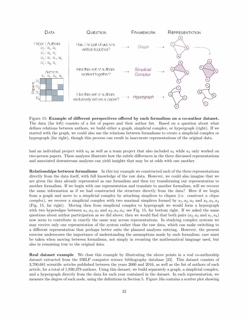
Figure 15: Example of different perspectives offered by each formalism on a co-author dataset.The data (far left) consists of a list of papers and their author list. Based on a question about whatdefines relations between authors, we build either a graph, simplicial complex, or hypergraph (right). If westarted with the graph, we could also use the relations between formalisms to create a simplicial complex orhypergraph (far right), though this process can result in inaccurate representations of the original data.

had an individual project with a2 as well as a team project that also included a3 while a4 only worked ontwo-person papers. These analyses illustrate how the subtle differences in the three discussed representationsand associated downstream analyses can yield insights that may be at odds with one another.

Relationships between formalisms In this toy example we constructed each of the three representationsdirectly from the data itself, with full knowledge of the raw data. However, we could also imagine that weare given the data already represented as one formalism and then try transforming our representation toanother formalism. If we begin with one representation and translate to another formalism, will we recoverthe same information as if we had constructed the structure directly from the data? Here if we beginfrom a graph and move to a simplicial complex by attaching simplices to cliques (i.e. construct a cliquecomplex ), we recover a simplicial complex with two maximal simplices formed by a1, a2, a3 and a2, a3, a4(Fig. 15, far right). Moving then from simplicial complex to hypergraph we would form a hypergraphwith two hyperedges between a1, a2, a3 and a2, a3, a4; see Fig. 15, far bottom right. If we asked the samequestions about author participation as we did above, then we would find that both pairs (a2, a3 and a1, a4)now seem to contribute in exactly the same way across representations. In studying complex systems wemay receive only one representation of the system rather than the raw data, which can make switching toa different representation that perhaps better suits the planned analyses enticing. However, the presentexercise underscores the importance of understanding the assumptions made by each formalism; care mustbe taken when moving between formalisms, not simply in recasting the mathematical language used, butalso in remaining true to the original data.

Real dataset example We close this example by illustrating the above points in a real co-authorshipdataset extracted from the DBLP computer science bibliography database [23]. This dataset consists of3,700,681 scientific articles published between the years 2000 and 2016, as well as the list of authors of eacharticle, for a total of 1,930,378 authors. Using this dataset, we build separately a graph, a simplicial complex,and a hypergraph directly from the data for each year contained in the dataset. In each representation, wemeasure the degree of each node, using the definitions in Section 5. Figure 16a contains a scatter plot showing

32

Figure 16: Correlation among degree measurements in different representations of the samedataset. (a) Comparing the degree calculated from the graph or hypergraph representation (left), fromthe simplicial complex or hypergraph representation (middle), and from the graph or simplicial complexrepresentation (right) from the co-authorship dataset extracted from the DBLP computer science bibliog-raphy database in year 2016. Correlation is relatively high for nodes of large degree, but relatively low fornodes of small degree. b Spearman correlation coefficient calculated between node degrees from pairs of datarepresentations in each year.

the degree of each node as measured in the different representations corresponding to year 2016. In thisdataset, the degree in any representation is positively correlated to the degree in any other representation,though progressively less so as the degree of the node decreases. This result means that the differentrepresentations often agree more on which nodes have the largest degrees than on which nodes have smalldegree. This is important to keep in mind, especially in studies that make claims about the nodes of smalldegree, which often outnumber those with large degree.

To see how this correlation changes over time, for each year we calculate the Spearman rank correlationcoefficient, which quantifies the similarity in node degree rankings between two representations. The Spear-man rank correlation coefficient is equal to 1.0 when the rankings are equal, and −1.0 when the rankings areexactly reversed. Shown in Fig. 16b, we measure this coefficient for each year and each pair of representations.We observe the highest correlation between degrees calculated from the simplicial complex representation(number of maximal simplices) and degrees calculated from the hypergraph representation (number of hy-peredges), which is likely due to the fact that these two representations both encode the polyadic relationsin the dataset. This result suggests that relatively few papers authored by a subset of the authors of anotherpaper were written. We also observe that the degrees calculated from the graph representations show a com-paratively low correlation to the node degrees calculated from the other representations. In particular, thecorrelation between the graph and the hypergraph drops below 0.5 in some years, signaling a very differentresult when ranking nodes by graph degree or by hypergraph degree. Our observations imply that, in thisdataset, we should be careful when making broad claims regarding the degree of nodes, especially those withfew observed relations (i.e. small degrees), as each representation may yield different results that must beinterpreted accordingly.

In summary, we have used this example to illustrate each step of the workflow from Figure 14, as well asto show that using different representations of the same dataset may yield measurements that are at odds

33

with each other, even in the simple case of measuring node degree and when the representations are createddirectly from the data.

6.2 Email communications

In our next example we again follow the the workflow of Fig. 14, but more succinctly. While in the previousexample we discussed multiple types of dependencies, variations in data availability, and differing researchquestions, here we provide an example of a seemingly straightforward analysis on a dataset of emails.

We start by considering the following scenario. Suppose Ana works at a company and is tasked withimproving communication and cohesiveness between teams in the workplace. Ana works at a big companythat contains many teams in diverse areas, so she decides to prioritize her involvement by focusing onaverage team communication via an easily accessible medium such as email. Concretely, Ana wants toevaluate how well each team integrates with all members of the company, which translates to evaluatingthe average clustering coefficient of each team. For this purpose, Ana has collected all the internal emailcommunications. She decides to operationalize her task as follows. First, if a set of at least 5 people have allreceived the same email at the same time, she will assume they must be working together as a team. Second,she decides to focus on emails with at most 25 participants, as emails with more than 25 participants are likelycompany-wide communications that do not involve a single team working together. Third, having identifieda team, she will quantify the team’s cohesiveness by averaging the clustering coefficient of each member in theteam. Note that in this system we represent no spatial dependencies as email allows instant communicationregardless of geographical location. Finally, Ana only cares about the teams and communication that havealready occurred, and is not hoping to predict communication in the future, so for the presented analysison aggregate communication she does not need to incorporate any temporal dependency that might existwithin the system.

To follow up with her plan, Ana needs to choose a formalism with which to encode the data, as wellas how to measure the clustering coefficient. If she chooses to encode the system as a graph where eachemployee is a node and each edge joins two nodes if they simultaneously received the same email, then shemay use the clustering coefficient defined in Section 5.1. Alternatively, she may choose to build a hypergraphwhere each node is an employee and each hyperedge denotes a single email, and use the clustering coefficientdefined in Section 5.3. A priori, one might expect that measuring the average clustering of a set of nodes inthe graph is highly correlated to measuring the same quantity in the hypergraph. However, we will see thatthe subtle differences in definitions lead to varying results.

For this example, we use a dataset of email communications [23], containing 10, 883 emails among 148employees of a company, from March 1999 to October 2002. Each email has a corresponding set of par-ticipants which includes the sender and all recipients. In Figure 17 we see the results of Ana’s analysis onthis dataset, using both a graph and a hypergraph representation of these data. Each marker represents anemail with between n and 25 participants, for n = 5, 6, 7, 8, i.e. what Ana considers to be a team. Eachemail is located according to the average clustering coefficient of the email’s participants, as measured inthe graph (horizontal axis) and in the hypergraph (vertical axis). In the top left panel we can see thatthere is very little correlation between these two quantities for teams of at least 5 people (Spearman rankcorrelation coefficient r = 0.1, and associated p-value p = 0.16). These results show that ranking teams ofemployees using these two different clustering coefficients yields very different results. Consequently, if Anawants to prioritize teams in order of how much she needs to intervene, in other words by ranking the teamsaccording to average clustering coefficient, then the graph and hypergraph representations will recommendvery different courses of action. Indeed, Ana would need to allocate her resources in entirely different waysdepending on which representation she chose. This result does not change if Ana chooses to focus on teamsof at least 6, 7, or 8 people, as shown in Fig 17.

Next, Ana decides to distinguish between team cohesiveness with the company and intra-team cohe-siveness. That is, do those teams that communicate well with everyone in the company also have robustwithin-team communication? A team that has excellent internal communication would have a high fill coeffi-cient, which measures the fraction of possible smaller hyperedges that exist between the nodes of a hyperedge(see Section 5.3). In order to answer this question Ana calculates the fill coefficient of each team and adds

34

Figure 17: Graph clustering and hypergraph clustering coefficients are loosely related. Fordifferent ranges of hyperedge cardinality, the average clustering coefficient of nodes within a hyperedgecalculated with the projected graph definition is compared to the average clustering coefficient calculatedfrom the hypergraph representation. Scatterplot points are colored by the log(fill coefficient).

35

this information as color on her scatterplots (Fig. 17). By eye her results show no relationship betweena team’s cohesiveness with the company (clustering coefficient calculated from the graph or hypergraphrepresentation) and a team’s internal cohesiveness (fill coefficient).

Together, these experiments illustrate that even in the case when a) the research question is fixed, b) theresearcher has access to the full dataset, and c) there are little-to-no interactions among different types ofdependencies, the choice of representation alone may still yield different insights by virtue of the differentassumptions made by each (here dyadic versus polyadic interactions).

7 Applications

We can naturally encode myriad systems in the real world with at least one of the formalisms discussed inthis work. Still, often we focus on analyzing a system from a particular perspective and spend less timeimagining how alternative analysis pipelines may be more revealing – or indeed more faithful to the system –than the currently used pipeline. Here we consider the alternative perspectives offered by the dependencies,formalisms, and challenges we have discussed in this paper.

First we consider the brain. The brain can be naturally conceived of as a system of individual partsthat work together to form large functional units at different scales: neurons work together to communicatewith each other forming co-firing patterns called code words [54], multiple neuronal populations collaboratein order to plan and evaluate trajectories [145], and entire brain regions work in unison to form functionalnetworks [81]. Scientists have successfully studied the brain by encoding it at any one of these scalesusing the representations discussed in this work [27]. For example, with graph representations researchersfound the brain to exhibit small-worldness [19, 15, 139], modular architecture [196, 81], and hubs [2, 3].Using the simplicial complex representation, at the larger scale cavities in the structural adult brain wereobserved [159, 191], and at a smaller scale researchers detected the geometric structure of pyramidal neuronfiring patterns [86]. Finally, research employing a hypergraph representation has identified functional hubhyperedges [219], characterized types of hyperedges in developing children [89], and tracked changes in brainorganization over both short [18, 56] and long time scales [57].

Looking to the future, one particularly little-understood aspect of the brain is the impact of temporaldependency. How do specific relations affect the existence of any other relations in the future? For example,can a brain transition from any arbitrary state to any other state [49], or is its future activity bound by itspast activity [12, 217]? Though the field has used temporal networks to investigate time-varying activity, atthe time of writing we did not find the inclusion of temporal dependencies within the representation. Wesuggest the application of higher-order network representations to deepen our understanding of temporaldependencies in this complex system. Additionally, at all scales the brain is spatially embedded [199],and previous work has shown that the strength of connections between brain regions often depends on theeuclidean distance between them [96, 170]. Often the analysis pipeline involves comparing any computedresults on the empirical data against a spatially-embedded null model [28], or co-modeling the spatial relationsand other relations such as by examining Rentian scaling [16, 97, 177]. While these approaches do helpto determine dependence of spatial features on other features, we suggest taking an additional step todirectly encoding spatial dependencies in the formal representation of the data. For example, multilayerrepresentations or sheaves encoding position information may be of help here.

Next we consider transportation, which is another well-studied system in network science. Transportationnetworks come in two different types: systems where the movement is done along fixed routes (such as roads,train tracks, power lines, or airline paths [171, 20, 183, 150, 47]), and systems where the movement is donefreely through (outer) space [173]. Among these, analyses specifically of public transportation networkshave incorporated multilayer networks [215] or variations thereof including internal node structure [186],and have also evaluated system-specific measures that include spatial organization [216]. Analyses involvingtemporal representations have included investigating congestion clusters in road networks [168] and how toalleviate them [102]. These analyses usually consider spatial and temporal dependencies by assigning weightsto the representation’s relations associated to distances or travel times [160, 181]. Importantly, studies arebeginning to encode the temporal dependency in the representation itself, as higher order networks have

36

revealed these temporal dependencies in data from global shipping and web browsing [223].The subset dependency is studied far less often than other types of dependencies in transportation

systems. For example, in a public transport system, if relations are defined among k stations if there existsa route X that stops at all k stations, then certainly any subset of those k stations must also be relatedby route X. Alternatively a subset dependency may or may not exist within traversed paths. For example,perhaps we observe paths of length k but we do not observe smaller sub-paths. How might the identificationor inclusion of subset dependencies within the transportation system improve our ability to prevent systemfailures or predict future activity? Additionally, we suggest further investigation of polyadic relations inthese systems with simplicial complexes or hypergraphs where appropriate, as these representations mayelucidate previously hidden system properties.

Finally we consider applications in cellular systems composed of any subset of proteins, genes, regulatoryunits such as enhancers, epigenetic factors, and more [77, 5]. Most commonly the field studies systemfragments such as genetic regulatory networks (GRNs) [60, 218, 70] and protein-protein interaction networks(PPINs) [61, 164]. Unlike the above two examples, this application differs in that only in rare situationscan real-world interactions be observed. Consequently, tremendous effort focuses on network reconstructionfrom data, i.e. inferring the interactions from indirect measurements [144, 213, 4]. Temporal informationsuch as fluctuations in RNA counts [194] and spatial information such as co-localization [127] can be used toreconstruct the network of interactions. Often, for example in the system fragment of proteins and proteincomplexes, polyadic relations exist and have been encoded using simplicial complexes or hypergraphs [163].Multilayer representations have also been used for representing multiple biological layers important in disease[92] and for inferring protein function [225].

The difficulties associated with macromolecule-interaction systems create an enticing problem for devel-oping system representations. Since the existence of interactions can rarely be observed directly, perhapsa representation with weights indicating the probability of the existence of each relation might be a usefulalternative. In such a case, one might consider studying an ensemble of graphs, simplicial complexes, orhypergraphs instead of only one, and differentiating among them based on the likelihood of each one beinga faithful representation of the real system. Additionally, though polyadic relations are known to play animportant role in these systems [205], simplicial complex and hypergraph representations are more rarelyemployed (examples include [73, 187, 111]. Finally, temporal fluctuations are becoming easier to record inthese systems [180], which poses the opportunity to directly study temporal dependencies.

8 Discussion and Conclusion

In this work we examined each step of a data analysis pipeline suitable for studying complex systems (Fig. 18).We first discussed system dependencies which can manifest in different flavors including but not limited totemporal, subset, and spatial. We then defined common complex system formalisms and their underlyingassumptions, as well as which dependencies they encode. We discussed the mathematical relationshipsbetween formalisms, and how information can be lost (or imputed) as we convert data from one formalismto another. Finally we offered analysis examples in order to underscore the importance of dependencies,careful choice of representation, and analysis techniques in studying complex systems.

The main message of our work is that there is no perfect way to analyze a system, and that studying twodifferent systems may require two entirely different pipelines. That is, the modeling decisions made whilestudying one dataset compiled from a system will not necessarily carry over to another system or, indeed,not even to another dataset extracted from the same system. In contrast, we see many studies apply certainpipelines for seemingly no other reason than because they are common within a certain field. Instead,we recommend that each new system and dataset be individually evaluated and investigated, and eachassumption and pipeline decision be made in accordance with the concepts discussed here. More specifically,and following Fig 18, we suggest designing pipelines based on the system and system dependencies, anyexternal dependencies that may be induced by the data type or data collection method, and the limits ofthe system fragment under study. From there, we suggest choosing a formalism that best fits the data, theresearch question, and the system itself, even if it requires using a new formalism or extension that is outside

37

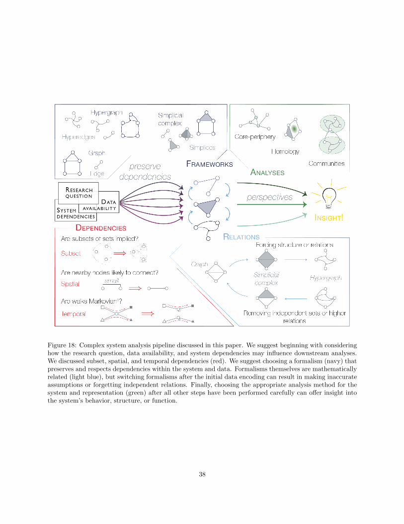
Figure 18: Complex system analysis pipeline discussed in this paper. We suggest beginning with consideringhow the research question, data availability, and system dependencies may influence downstream analyses.We discussed subset, spatial, and temporal dependencies (red). We suggest choosing a formalism (navy) thatpreserves and respects dependencies within the system and data. Formalisms themselves are mathematicallyrelated (light blue), but switching formalisms after the initial data encoding can result in making inaccurateassumptions or forgetting independent relations. Finally, choosing the appropriate analysis method for thesystem and representation (green) after all other steps have been performed carefully can offer insight intothe system’s behavior, structure, or function.

38

of what is customary. Finally, we recommend choosing carefully the specific methods, measurements, andanalyses performed on the chosen representation, and keeping in mind that their results may be biased bythe choices made in the previous stages. Different choices at each of these steps may ultimately yield resultsthat are at odds with the results yielded by other choices. Only after respecting the system’s dependenciesand unique qualities through proper representation and analysis methods will we uncover novel insight intothe system under study.

Though here we present only a first attempt to unify the application of complex systems analyses, wehope that the drive for more accurate representations will continue to push the field both forward andcloser together through multiplying collaborations. We imagine that complex systems researchers in thefuture may each have a slew of representations along with carefully chosen computations that respect thedependencies one finds within the system. By continuing this discussion, the separate areas of science thatuse complex systems analyses will together identify what is missing from current formalisms, create moreinsightful analyses, and generate novel techniques.

9 Acknowledgments

First and foremost, we wish to acknowledge the colleagues, co-authors, mentors, and mentees who haveshaped our perspective on this subject. Next, we wish to thank Jason Kim, Linden Parkes, and ShubhankarPatankar for their helpful and constructive comments on an earlier version of this manuscript. Finally,we acknowledge critical financial support that allowed us to devote time to this work. ASB and DSB ac-knowledge support from the Army Research Office (Falk-W911NF-18-1-0244, Grafton-W911NF-16-1-0474,DCIST- W911NF-17-2-0181), the National Science foundation (PHY-1554488, IIS-1926757), and the PaulG. Allen Family Foundation. LT and TER were supported in part by the National Science Foundation(IIS-1741197) and by the Combat Capabilities Development Command Army Research Laboratory (underCooperative Agreement Number W911NF-13-2-0045). The views and conclusions contained in this doc-ument are those of the authors and should not be interpreted as representing the official policies, eitherexpressed or implied, of the Combat Capabilities Development Command Army Research Laboratory or theU.S. Government. The U.S. Government is authorized to reproduce and distribute reprints for Governmentpurposes not withstanding any copyright notation here.

10 Citation diversity statement

Recent work in several fields of science has identified a bias in citation practices such that papers from womenand other minorities are under-cited relative to the number of such papers in the field [67, 126, 38, 42, 206, 63].Here we sought to proactively consider choosing references that reflect the diversity of the field in thought,form of contribution, gender, and other factors. Gender bias can arise due to explicit and implicit biasagainst a person’s known gender as a woman, or due to explicit or implicit bias against a person carrying aname commonly used by women [123, 152, 137]. To evaluate the former (bias according to known gender),we obtained predicted gender of the first and last author of each reference using pronouns affiliated withthem online or pronouns known by personal friendships; by this measure (and excluding self-citations tothe first and last authors of our current paper), our references contain 42% man(first)/man(last), 13%man/woman, 10% woman/man, 13% woman/woman, 0% non-binary , and 21% unknown categorization.This method is limited in that pronouns may not be indicative of gender identity, and may not be consistentacross time or environment. To evaluate the latter (bias according to a gendered name), we used databasesthat store the probability of a name being carried by a woman; by this measure (again excluding self-citations), our references contains 60% man/man names, 12% man/woman names, 11% woman/man names,10% woman/woman names, and 7% unknown categorization [227, 67]. This method is limited in that itcannot account for intersex, non-binary, or transgender people. We look forward to future work that couldhelp us to better understand how to support equitable practices in science.

39

References

[1] The Apache Software Foundation 2020. Apache airflow. https://airflow.apache.org/. Accessed:2020-05-22.

[2] Sophie Achard, C Delon-Martin, P E Vertes, F Renard, M Schenck, F Schneider, C Heinrich, S Kremer,and Edward T Bullmore. Hubs of brain functional networks are radically reorganized in comatosepatients. Proceedings of the National Academy of Sciences USA, 109(50):20608–13, 2012.

[3] Sophie Achard, R Salvador, B Whitcher, John Suckling, and Edward Bullmore. A resilient, low-frequency, small-world human brain functional network with highly connected association corticalhubs. Journal of Neuroscience, 26(1):63–72, 2006.

[4] Reka Albert. Network inference, analysis, and modeling in systems biology. The Plant Cell,19(11):3327–3338, 2007.

[5] Uri Alon. Network motifs: theory and experimental approaches. Nature Reviews Genetics, 8(6):450–461, 2007.

[6] Luıs A Nunes Amaral, Antonio Scala, Marc Barthelemy, and H Eugene Stanley. Classes of small-worldnetworks. Proceedings of the National Academy of Sciences USA, 97(21):11149–11152, 2000.

[7] Andrea Apolloni, C Poletto, and Vittoria Colizza. Age-specific contacts and travel patterns in thespatial spread of 2009 H1N1 influenza pandemic. BMC Infectious Diseases, 13:176, 2013.

[8] Viplove Arora and Mario Ventresca. Action-based modeling of complex networks. Scientific Reports,7(1):1–10, 2017.

[9] Ronald H Atkin. From cohomology in physics to q-connectivity in social science. International Journalof Man-Machine Studies, 4(2):139–167, 1972.

[10] Albert-Laszlo Barabasi and Reka Albert. Emergence of scaling in random networks. Science,286(5439):509–512, 1999.

[11] Matteo Barigozzi, Giorgio Fagiolo, and Giuseppe Mangioni. Identifying the community structure of theinternational-trade multi-network. Physica A: Statistical Mechanics and its Applications, 390(11):2051–2066, 2011.

[12] Anna Barnes, Edward T Bullmore, and John Suckling. Endogenous human brain dynamics recoverslowly following cognitive effort. PLoS One, 4(8):e6626, 2009.

[13] Marc Barthelemy. Spatial networks. Physics Reports, 499(1-3):1–101, 2011.

[14] Marc Barthelemy. Transitions in spatial networks. Comptes Rendus Physique, 19(4):205–232, 2018.

[15] Danielle S Bassett and Edward T Bullmore. Small-world brain networks revisited. Neuroscientist,23(5):499–516, 2017.

[16] Danielle S Bassett, Daniel L Greenfield, Andreas Meyer-Lindenberg, Daniel R Weinberger, Simon WMoore, and Edward T Bullmore. Efficient physical embedding of topologically complex informationprocessing networks in brains and computer circuits. PLoS Computational Biology, 6(4):e1000748,2010.

[17] Danielle S Bassett and Olaf Sporns. Network neuroscience. Nature Neuroscience, 20(3):353, 2017.

[18] Danielle S. Bassett, Nicholas F. Wymbs, Mason A. Porter, Peter J. Mucha, and Scott T Grafton.Cross-linked structure of network evolution. Chaos, 24(1):013112, 2014.

40

[19] Danielle Smith Bassett and Edward T Bullmore. Small-world brain networks. The Neuroscientist,12(6):512–523, 2006.

[20] Hannah Bast, Daniel Delling, Andrew Goldberg, Matthias Muller-Hannemann, Thomas Pajor, PeterSanders, Dorothea Wagner, and Renato F Werneck. Route planning in transportation networks. InAlgorithm Engineering, pages 19–80. Springer, 2016.

[21] Federico Battiston, Giulia Cencetti, Iacopo Iacopini, Vito Latora, Maxime Lucas, Alice Patania, Jean-Gabriel Young, and Giovanni Petri. Networks beyond pairwise interactions: Structure and dynamics.Physics Reports, 2020.

[22] Alex Bavelas. Communication patterns in task-oriented groups. The Journal of the Acoustical Societyof America, 22(6):725–730, 1950.

[23] Austin R. Benson, Rediet Abebe, Michael T. Schaub, Ali Jadbabaie, and Jon M. Kleinberg. Simpli-cial closure and higher-order link prediction. Proceedings of the National Academy of Sciences USA,115(48):E11221–E11230, 2018.

[24] Austin R Benson, David F Gleich, and Jure Leskovec. Higher-order organization of complex networks.Science, 353(6295):163–166, 2016.

[25] Austin R Benson, Ravi Kumar, and Andrew Tomkins. Sequences of sets. In Proceedings of the 24thACM SIGKDD International Conference on Knowledge Discovery and Data Mining KDD, 2018.

[26] Claude Berge. Hypergraphs: Combinatorics of Finite Sets, volume 45. Elsevier, 1984.

[27] Richard F. Betzel and Danielle S. Bassett. Multi-scale brain networks. NeuroImage, 160:73–83, 2017.

[28] Richard F. Betzel, John D. Medaglia, Lia Papadopoulos, Graham L Baum, Ruben Gur, Raquel Gur,David Roalf, Theodore D Satterthwaite, and Danielle S Bassett. The modular organization of humananatomical brain networks: Accounting for the cost of wiring. Network Neuroscience, 1(1):42–68, 2017.

[29] Ginestra Bianconi. Multilayer Networks: Structure and Function. Oxford University Press, 2018.

[30] Jacob Charles Wright Billings, Mirko Hu, Giulia Lerda, Alexey N Medvedev, Francesco Mottes, AdrianOnicas, Andrea Santoro, and Giovanni Petri. Simplex2vec embeddings for community detection insimplicial complexes. arXiv preprint arXiv:1906.09068, 2019.

[31] Stefano Boccaletti, Ginestra Bianconi, Regino Criado, Charo I Del Genio, Jesus Gomez-Gardenes,Miguel Romance, Irene Sendina-Nadal, Zhen Wang, and Massimiliano Zanin. The structure anddynamics of multilayer networks. Physics Reports, 544(1):1–122, 2014.

[32] Stephen P Borgatti and Martin G Everett. Models of core/periphery structures. Social Networks,21(4):375–395, 2000.

[33] Christian Borgs and Jennifer Chayes. Graphons: A nonparametric method to model, estimate, anddesign algorithms for massive networks. In Proceedings of the 2017 ACM Conference on Economicsand Computation, pages 665–672. ACM, 2017.

[34] Rotem Botvinik-Nezer, Felix Holzmeister, Colin F Camerer, Anna Dreber, Juergen Huber, MagnusJohannesson, Michael Kirchler, Roni Iwanir, Jeanette A Mumford, R Alison Adcock, et al. Variabilityin the analysis of a single neuroimaging dataset by many teams. Nature, pages 1–7, 2020.

[35] Charles D Brummitt, Raissa M. D’Souza, and Elizabeth A. Leicht. Suppressing cascades of load ininterdependent networks. Proceddings of the National Academy of Sciences USA, 109(12):E680–E689,2012.

41

[36] Edward T. Bullmore and Olaf Sporns. Complex brain networks: graph theoretical analysis of structuraland functional systems. Nature Reviews Neuroscience, 10(3):186, 2009.

[37] Carter T Butts. Revisiting the foundations of network analysis. Science, 325(5939):414–416, 2009.

[38] Neven Caplar, Sandro Tacchella, and Simon Birrer. Quantitative evaluation of gender bias in astro-nomical publications from citation counts. Nature Astronomy, 1(6):1–5, 2017.

[39] Gunnar Carlsson. Topology and data. Bulletin of the American Mathematical Society, 46(2):255–308,2009.

[40] Gunnar Carlsson, Tigran Ishkhanov, Vin De Silva, and Afra Zomorodian. On the local behavior ofspaces of natural images. International Journal of Computer Vision, 76(1):1–12, 2008.

[41] Deepayan Chakrabarti, Yang Wang, Chenxi Wang, Jure Leskovec, and Christos Faloutsos. Epidemicthresholds in real networks. ACM Transactions on Information and System Security, 10(4):1:1–1:26,2008.

[42] Paula Chakravartty, Rachel Kuo, Victoria Grubbs, and Charlton McIlwain. #CommunicationSoWhite.Journal of Communication, 68(2):254–266, 2018.

[43] Philip Chodrow and Andrew Mellor. Annotated hypergraphs: Models and applications. AppliedNetwork Science, 5(1):9, 2020.

[44] Philip S Chodrow, Z Al-Awwad, S Jiang, and Marta C Gonzalez. Demand and congestion in multiplextransportation networks. PLoS One, 11(9):e0161738, 2016.

[45] Phillip Christie and Dirk Stroobandt. The interpretation and application of rent’s rule. IEEE Trans-actions on Very Large Scale Integration (VLSI) Systems, 8(6):639–648, 2000.

[46] Aaron Clauset, Daniel B Larremore, and Roberta Sinatra. Data-driven predictions in the science ofscience. Science, 355(6324):477–480, 2017.

[47] Vittoria Colizza, Alain Barrat, Marc Barthelemy, and Alessandro Vespignani. The role of the airlinetransportation network in the prediction and predictability of global epidemics. Proceedings of theNational Academy of Sciences USA, 103(7):2015–2020, 2006.

[48] Vittoria Colizza and Alessandro Vespignani. Epidemic modeling in metapopulation systems withheterogeneous coupling pattern: Theory and simulations. Journal of Theoretical Biology, 251(3):450–467, 2008.

[49] Eli J. Cornblath, Arian Ashourvan, Jason Z Kim, Richard F. Betzel, Rastko Ciric, Azeez Adebimpe,Graham L Baum, Xiaosong He, Kosha Ruparel, Tyler M Moore, Ruben C Gur, Raquel E Gur, Russel TShinohara, David R Roalf, Theodore D Satterthwaite, and Danielle S Bassett. Temporal sequences ofbrain activity at rest are constrained by white matter structure and modulated by cognitive demands.Communications Biology, 3(1):261, 2020.

[50] L da F Costa, Francisco A Rodrigues, Gonzalo Travieso, and Paulino Ribeiro Villas Boas. Char-acterization of complex networks: A survey of measurements. Advances in Physics, 56(1):167–242,2007.

[51] O T Courtney and G Bianconi. Dense power-law networks and simplicial complexes. Physical ReviewE, 97(5-1):052303, 2018.

[52] Justin M. Curry. Sheaves, Cosheaves and Their Applications. PhD thesis, University of Pennsylvania,2014.

42

[53] Carina Curto. What can topology tell us about the neural code? Bulletin of the American MathematicalSociety, 54(1):63–78, 2017.

[54] Carina Curto, Elizabeth Gross, Jack Jeffries, Katherine Morrison, Mohamed Omar, Zvi Rosen, AnneShiu, and Nora Youngs. What makes a neural code convex? SIAM Journal on Applied Algebra andGeometry, 1(1):222–238, 2017.

[55] David B Damiano and Melissa R McGuirl. A topological analysis of targeted in-111 uptake in spectimages of murine tumors. Journal of Mathematical Biology, 76(6):1559–1587, 2018.

[56] Elizabeth N Davison, Kimberly J Schlesinger, Danielle S Bassett, Mary-Ellen Lynall, Michael B Miller,Scott T Grafton, and Jean M Carlson. Brain network adaptability across task states. PLoS Compu-tational Biology, 11(1):e1004029., 2015.

[57] Elizabeth N Davison, B O Turner, Kimberly J Schlesinger, Michael B Miller, Scott T Grafton,Danielle S Bassett, and Jean M Carlson. Individual differences in dynamic functional brain con-nectivity across the human lifespan. PLoS Computational Biology, 12(11):e1005178, 2016.

[58] Manlio De Domenico, Clara Granell, Mason A Porter, and Alex Arenas. The physics of spreadingprocesses in multilayer networks. Nature Physics, 12(10):901, 2016.

[59] Manlio De Domenico, Andrea Lancichinetti, Alex Arenas, and Martin Rosvall. Identifying modu-lar flows on multilayer networks reveals highly overlapping organization in interconnected systems.Physical Review X, 5(1):011027, 2015.

[60] Hidde De Jong. Modeling and simulation of genetic regulatory systems: a literature review. Journalof Computational Biology, 9(1):67–103, 2002.

[61] Javier De Las Rivas and Celia Fontanillo. Protein–protein interactions essentials: key concepts tobuilding and analyzing interactome networks. PLoS Computational Biology, 6(6), 2010.

[62] Andrea De Montis, Marc Barthelemy, Alessandro Chessa, and Alessandro Vespignani. The structure ofinterurban traffic: a weighted network analysis. Environment and Planning B: Planning and Design,34(5):905–924, 2007.

[63] Michelle L Dion, Jane Lawrence Sumner, and Sara McLaughlin Mitchell. Gendered citation patternsacross political science and social science methodology fields. Political Analysis, 26(3):312–327, 2018.

[64] Clifford H Dowker. Homology groups of relations. Annals of Mathematics, pages 84–95, 1952.

[65] Raissa M. D’Souza, Jesus Gomez-Gardenes, Jan Nagler, and Alex Arenas. Explosive phenomena incomplex networks. Advances in Physics, 68(3):123–223, 2019.

[66] Olga Dunaeva, Herbert Edelsbrunner, Anton Lukyanov, Michael Machin, Daria Malkova, RomanKuvaev, and Sergey Kashin. The classification of endoscopy images with persistent homology. PatternRecognition Letters, 83:13–22, 2016.

[67] Jordan D Dworkin, Kristin A Linn, Erin G Teich, Perry Zurn, Russell T Shinohara, and Danielle S Bas-sett. The extent and drivers of gender imbalance in neuroscience reference lists. Nature Neuroscience,23, 2020.

[68] Herbert Edelsbrunner, David Letscher, and Afra Zomorodian. Topological persistence and simplifica-tion. In Proceedings. 41st Annual Symposium on Foundations of Computer Science, pages 454–463.IEEE, 2000.

[69] Daniel Edler, Ludvig Bohlin, et al. Mapping higher-order network flows in memory and multilayernetworks with infomap. Algorithms, 10(4):112, 2017.

43

[70] Frank Emmert-Streib, Matthias Dehmer, and Benjamin Haibe-Kains. Gene regulatory networks andtheir applications: understanding biological and medical problems in terms of networks. Frontiers inCell and Developmental Biology, 2:38, 2014.

[71] Ernesto Estrada, Gissell Estrada-Rodriguez, and Heiko Gimperlein. Metaplex networks: influence ofthe exo-endo structure of complex systems on diffusion. SIAM Review, 62(3), 2020.

[72] Ernesto Estrada and Juan A Rodrıguez-Velazquez. Subgraph centrality and clustering in complexhyper-networks. Physica A: Statistical Mechanics and its Applications, 364:581–594, 2006.

[73] Ernesto Estrada and Grant J Ross. Centralities in simplicial complexes. Applications to protein inter-action networks. Journal of Theoretical Biology, 438:46–60, 2018.

[74] Leonhard Euler. Solutio problematis ad geometriam situs pertinentis. Commentarii academiae scien-tiarum Petropolitanae, pages 128–140, 1741.

[75] Shimon Even. Graph Algorithms. Cambridge University Press, 2011.

[76] Paul Expert, Tim S Evans, Vincent D Blondel, and Renaud Lambiotte. Uncovering space-independentcommunities in spatial networks. Proceedings of the National Academy of Sciences USA, 108(19):7663–7668, 2011.

[77] Valeria Fionda. Networks in Biology. Elsevier, 2019.

[78] Linton Freeman. The Development of Social Network Analysis: A Study in the Sociology of Science.Empirical press, 2004.

[79] Linton C Freeman. A set of measures of centrality based on betweenness. Sociometry, pages 35–41,1977.

[80] Suzanne Renick Gallagher and Debra S Goldberg. Clustering coefficients in protein interaction hyper-networks. In Proceedings of the International Conference on Bioinformatics, Computational Biologyand Biomedical Informatics, pages 552–560, 2013.

[81] C L Gallen and M D’Esposito. Brain modularity: A biomarker of intervention-related plasticity. Trendsin Cognitive Science, 23(4):293–304, 2019.

[82] Giorgio Gallo, Giustino Longo, Stefano Pallottino, and Sang Nguyen. Directed hypergraphs andapplications. Discrete Applied Mathematics, 42(2-3):177–201, 1993.

[83] Robert Ghrist. Barcodes: the persistent topology of data. Bulletin of the American MathematicalSociety, 45(1):61–75, 2008.

[84] Robert Ghrist and Yasuaki Hiraoka. Applications of sheaf cohomology and exact sequences to networkcoding. In Proceedings of the 2011 Nonlinear Theory and its Applications. NOLTA, 2011.

[85] Chad Giusti, Robert Ghrist, and Danielle S Bassett. Two’s company, three (or more) is a simplex.Journal of computational neuroscience, 41(1):1–14, 2016.

[86] Chad Giusti, Eva Pastalkova, Carina Curto, and Vladimir Itskov. Clique topology reveals intrinsicgeometric structure in neural correlations. Proceedings of the National Academy of Sciences USA,112(44):13455–13460, 2015.

[87] Stefania Gnesi, Ugo Montanari, and Alberto Martelli. Dynamic programming as graph searching: Analgebraic approach. Journal of the ACM (JACM), 28(4):737–751, 1981.

[88] Deanna J Greene, Christina N Lessov-Schlaggar, and Bradley L Schlaggar. Development of the brain’sfunctional network architecture. In Neurobiology of Language, pages 399–406. Elsevier, 2016.

44

[89] Shi Gu, Muzhi Yang, John D Medaglia, Ruben C Gur, Raquel E Gur, Theodore D Satterthwaite, andDanielle S Bassett. Functional hypergraph uncovers novel covariant structures over neurodevelopment.Human Brain Mapping, 38(8):3823–3835, 2017.

[90] Roger Guimera, Marta Sales-Pardo, and Luıs A Nunes Amaral. Modularity from fluctuations inrandom graphs and complex networks. Physical Review E, 70(2):025101, 2004.

[91] Mahnaz Habibi and Pegah Khosravi. Disruption of the protein complexes from weighted complexnetworks. IEEE/ACM Transactions on Computational Biology and Bioinformatics, 2018.

[92] Arda Halu, Manlio De Domenico, Alex Arenas, and Amitabh Sharma. The multiplex network ofhuman diseases. NPJ Systems Biology and Applications, 5(1):1–12, 2019.

[93] Ilkka Hanski. Metapopulation Ecology. Oxford University Press, 1999.

[94] Frank Harary and Robert Z Norman. Some properties of line digraphs. Rendiconti del Circolo Matem-atico di Palermo, 9(2):161–168, 1960.

[95] Petter Holme and Jari Saramaki. Temporal networks. Physics Reports, 519(3):97–125, 2012.

[96] Szabolcs Horvat, Razvan Gamanut, , Maria Ercsey-Ravasz, Loıc Magrou, Bianca Gamanut, , David CVan Essen, Andreas Burkhalter, Kenneth Knoblauch, Zoltan Toroczkai, and Henry Kennedy. Spatialembedding and wiring cost constrain the functional layout of the cortical network of rodents andprimates. PLoS Biology, 14(7):e1002512, 2016.

[97] Javier J How and Saket Navlakha. Evidence of rentian scaling of functional modules in diverse biologicalnetworks. Neural Computation, 30(8):2210–2244, 2018.

[98] Sen Hu, Hualei Yang, Boliang Cai, and Chunxia Yang. Research on spatial economic structure fordifferent economic sectors from a perspective of a complex network. Physica A: Statistical Mechanicsand its Applications, 392(17):3682–3697, 2013.

[99] Iacopo Iacopini, Giovanni Petri, Alain Barrat, and Vito Latora. Simplicial models of social contagion.Nature Communications, 10(1):1–9, 2019.

[100] Paul Samuel P Ignacio and Isabel K Darcy. Tracing patterns and shapes in remittance and migrationnetworks via persistent homology. EPJ Data Science, 8(1):1, 2019.

[101] Bukyoung Jhun, Minjae Jo, and B Kahng. Simplicial sis model in scale-free uniform hypergraph.Journal of Statistical Mechanics: Theory and Experiment, 2019(12):123207, 2019.

[102] Yuxuan Ji and Nikolas Geroliminis. Spatial and temporal analysis of congestion in urban transportationnetworks. In Transportation Research Board Annual Meeting. Washington DC, 2011.

[103] Christopher W Johnson. What are emergent properties and how do they affect the engineering ofcomplex systems? Reliability Engineering and System Safety, 91(12):1475–1481, 2006.

[104] Matthew Kahle. Topology of random clique complexes. Discrete Mathematics, 309(6):1658–1671, 2009.

[105] Matthew Kahle. Sharp vanishing thresholds for cohomology of random flag complexes. Annals ofMathematics, pages 1085–1107, 2014.

[106] Ankit N Khambhati, Ann E Sizemore, Richard F Betzel, and Danielle S Bassett. Modeling andinterpreting mesoscale network dynamics. NeuroImage, 180:337–349, 2018.

[107] Chiheon Kim, Afonso S Bandeira, and Michel X Goemans. Community detection in hypergraphs,spiked tensor models, and sum-of-squares. In 2017 International Conference on Sampling Theory andApplications (SampTA), pages 124–128. IEEE, 2017.

45

[108] Mikko Kivela, Alex Arenas, Marc Barthelemy, James P Gleeson, Yamir Moreno, and Mason A Porter.Multilayer networks. Journal of Complex Networks, 2(3):203–271, 2014.

[109] Sophia Kivelson and Steven A Kivelson. Defining emergence in physics. Nature Partner JournalsQuantum Materials, 1:16024, 2016.

[110] Steffen Klamt and Ernst Dieter Gilles. Minimal cut sets in biochemical reaction networks. Bioinfor-matics, 20(2):226–234, 2004.

[111] Steffen Klamt, Utz-Uwe Haus, and Fabian Theis. Hypergraphs and cellular networks. PLoS Compu-tational Biology, 5(5), 2009.

[112] Michael Kotliar, Andrey V Kartashov, and Artem Barski. Cwl-airflow: a lightweight pipeline managersupporting common workflow language. GigaScience, 8(7):giz084, 2019.

[113] Larkshmi Krishnamurthy, J Nadeau, Gultekin Ozsoyoglu, M Ozsoyoglu, Greg Schaeffer, Murat Tasan,and Wanhong Xu. Pathways database system: an integrated system for biological pathways. Bioin-formatics, 19(8):930–937, 2003.

[114] Florent Krzakala, Cristopher Moore, Elchanan Mossel, Joe Neeman, Allan Sly, Lenka Zdeborova, andPan Zhang. Spectral redemption in clustering sparse networks. Proceedings of the National Academyof Sciences USA, 110(52):20935–20940, 2013.

[115] James Ladyman and Karoline Wiesner. What is a complex system? Yale University Press, 2020.

[116] Eric C Lai. Notch signaling: control of cell communication and cell fate. Development, 131(5):965–973,2004.

[117] Renaud Lambiotte, Martin Rosvall, and Ingo Scholtes. From networks to optimal higher-order modelsof complex systems. Nature Physics, page 1, 2019.

[118] Renaud Lambiotte, Vsevolod Salnikov, and Martin Rosvall. Effect of memory on the dynamics ofrandom walks on networks. Journal of Complex Networks, 3(2):177–188, 2014.

[119] Giorgio Levi and Franco Sirovich. Generalized and/or graphs. Artificial Intelligence, 7(3):243–259,1976.

[120] Richard Levins. Some demographic and genetic consequences of environmental heterogeneity for bio-logical control. American Entomologist, 15(3):237–240, 1969.

[121] Jiaqi Liang, L Li, and Daniel Zeng. Evolutionary dynamics of cryptocurrency transaction networks:An empirical study. PLoS One, 13(8):e0202202, 2018.

[122] Antonio Lima, R Stanojevic, D Papagiannaki, P Rodriguez, and Marta C Gonzalez. Understandingindividual routing behaviour. Journal of the Royal Society Interface, 13(116):20160021, 2016.

[123] Lillian MacNell, Adam Driscoll, and Andrea N Hunt. What’s in a name: Exposing gender bias instudent ratings of teaching. Innovative Higher Education, 40(4):291–303, 2015.

[124] Parul Maheshwari, H Du, J Sheen, S M Assmann, and Reka Albert. Model-driven discovery of calcium-related protein-phosphatase inhibition in plant guard cell signaling. PLoS Computational Biology,15(10):e1007429, 2019.

[125] Slobodan Maletic, Milan Rajkovic, and Danijela Vasiljevic. Simplicial complexes of networks and theirstatistical properties. In International Conference on Computational Science, pages 568–575. Springer,2008.

46

[126] Daniel Maliniak, Ryan Powers, and Barbara F Walter. The gender citation gap in internationalrelations. International Organization, 67(4):889–922, 2013.

[127] Faraz K Mardakheh, Heba Z Sailem, Sandra Kumper, Christopher J Tape, Ryan R McCully, AngelaPaul, Sara Anjomani-Virmouni, Claus Jørgensen, George Poulogiannis, Christopher J Marshall, et al.Proteomics profiling of interactome dynamics by colocalisation analysis (cola). Molecular BioSystems,13(1):92–105, 2017.

[128] Ken McRae, George S Cree, Mark S Seidenberg, and Chris McNorgan. Semantic feature productionnorms for a large set of living and nonliving things. Behavior Research Methods, 37(4):547–559, 2005.

[129] Giulia Menichetti, L Dall’Asta, and Ginestra Bianconi. Control of multilayer networks. Sci Rep,6:20706, 2016.

[130] Giulia Menichetti, Daniel Remondini, Pietro Panzarasa, Raul J Mondragon, and Ginestra Bianconi.Weighted multiplex networks. PloS One, 9(6):e97857, 2014.

[131] Nikola Milosavljevic, Dmitriy Morozov, and Primoz Skraba. Zigzag persistent homology in matrixmultiplication time. In Proceedings of the Twenty-Seventh Annual Symposium on Computational Ge-ometry, pages 216–225. ACM, 2011.

[132] Melanie Mitchell. Complex systems: Network thinking. Artificial Intelligence, 170(18):1194–1212,2006.

[133] Melanie Mitchell. Complexity: A Guided Tour. Oxford University Press, 2009.

[134] Michael Molloy and Bruce Reed. A critical point for random graphs with a given degree sequence.Random Structures & Algorithms, 6(2-3):161–180, 1995.

[135] Jose M Montoya, Stuart L Pimm, and Ricard V Sole. Ecological networks and their fragility. Nature,442(7100):259, 2006.

[136] Katherine Morrison and Carina Curto. Predicting neural network dynamics via graphical analysis. InAlgebraic and Combinatorial Computational Biology, pages 241–277. Elsevier, 2019.

[137] Corinne A Moss-Racusin, John F Dovidio, Victoria L Brescoll, Mark J Graham, and Jo Handelsman.Science faculty’s subtle gender biases favor male students. Proceedings of the National Academy ofSciences USA, 109(41):16474–16479, 2012.

[138] Peter J Mucha, Thomas Richardson, Kevin Macon, Mason A Porter, and Jukka-Pekka Onnela. Com-munity structure in time-dependent, multiscale, and multiplex networks. Science, 328(5980):876–878,2010.

[139] Sarah F. Muldoon, Eric W. Bridgeford, and Danielle S. Bassett. Small-world propensity and weightedbrain networks. Scientific Reports, 6:22057, 2016.

[140] Andrew C Murphy, Shi Gu, Ankit N Khambhati, Nicholas F Wymbs, Scott T Grafton, Theodore DSatterthwaite, and Danielle S Bassett. Explicitly linking regional activation and function con-nectivity: community structure of weighted networks with continuous annotation. arXiv preprintarXiv:1611.07962, 2016.

[141] Nicolas Neubauer and Klaus Obermayer. Towards community detection in k-partite k-uniform hyper-graphs. In Proceedings of the NIPS 2009 Workshop on Analyzing Networks and Learning with Graphs,pages 1–9, 2009.

[142] Mark Newman. Networks. Oxford university press, 2018.

47

[143] Vincenzo Nicosia, John Tang, Cecilia Mascolo, Mirco Musolesi, Giovanni Russo, and Vito Latora.Graph metrics for temporal networks. In Temporal Networks, pages 15–40. Springer, 2013.

[144] Chris J Oates and Sach Mukherjee. Network inference and biological dynamics. The Annals of AppliedStatistics, 6(3):1209, 2012.

[145] H Freyja Olafsdottir, Daniel Bush, and Caswell Barry. The role of hippocampal replay in memory andplanning. Current Biology, 28(1):R37–R50, 2018.

[146] Jukka-Pekka Onnela, Daniel J Fenn, Stephen Reid, Mason A Porter, Peter J Mucha, Mark D Fricker,and Nick S Jones. Taxonomies of networks from community structure. Physical Review E, 86(3):036104,2012.

[147] Edward Ott, J H Platig, T M Antonsen, and Michelle Girvan. Echo phenomena in large systems ofcoupled oscillators. Chaos, 18(3):037115, 2008.

[148] Nina Otter, Mason A Porter, U Tillmann, P Grindrod, and Heather A Harrington. A roadmap for thecomputation of persistent homology. EPJ Data Science, 6(1):17, 2017.

[149] Can Ozturan. On finding hypercycles in chemical reaction networks. Applied Mathematics Letters,21(9):881–884, 2008.

[150] Giuliano Andrea Pagani and Marco Aiello. The power grid as a complex network: a survey. PhysicaA: Statistical Mechanics and its Applications, 392(11):2688–2700, 2013.

[151] Gergely Palla, Imre Derenyi, Illes Farkas, and Tamas Vicsek. Uncovering the overlapping communitystructure of complex networks in nature and society. Nature, 435(7043):814, 2005.

[152] Michele A Paludi and Lisa A Strayer. What’s in an author’s name? differential evaluations of perfor-mance as a function of author’s name. Sex Roles, 12(3-4):353–361, 1985.

[153] Joshua Pan, Robin M Meyers, Brittany C Michel, Nazar Mashtalir, Ann E Sizemore, Jonathan NWells, Seth H Cassel, Francisca Vazquez, Barbara A Weir, William C Hahn, et al. Interrogation ofmammalian protein complex structure, function, and membership using genome-scale fitness screens.Cell Systems, 6(5):555–568, 2018.

[154] Lia Papadopoulos, Pablo Blinder, Henrik Ronellenfitsch, Florian Klimm, Eleni Katifori, David Klein-feld, and Danielle S Bassett. Comparing two classes of biological distribution systems using networkanalysis. PLoS Computational Biology, 14(9):e1006428, 2018.

[155] Lia Papadopoulos, Jason Z Kim, Jurgen Kurths, and Danielle S Bassett. Development of structuralcorrelations and synchronization from adaptive rewiring in networks of kuramoto oscillators. Chaos:An Interdisciplinary Journal of Nonlinear Science, 27(7):073115, 2017.

[156] Lia Papadopoulos, Mason A Porter, Karen E Daniels, and Danielle S Bassett. Network analysis ofparticles and grains. Journal of Complex Networks, 6(4):485–565, 2018.

[157] Jorge Pena and Yannick Rochat. Bipartite graphs as models of population structures in evolutionarymultiplayer games. PloS One, 7(9), 2012.

[158] Vincenzo Perri and Ingo Scholtes. Higher-order visualization of causal structures in dynamics graphs.arXiv preprint arXiv:1908.05976, 2019.

[159] Giovanni Petri, Paul Expert, Federico Turkheimer, Robin Carhart-Harris, David Nutt, Peter J Hellyer,and Francesco Vaccarino. Homological scaffolds of brain functional networks. Journal of The RoyalSociety Interface, 11(101):20140873, 2014.

48

[160] Sergio Porta, Paolo Crucitti, and Vito Latora. The network analysis of urban streets: a primalapproach. Environment and Planning B: Planning and Design, 33(5):705–725, 2006.

[161] Stephen R Proulx, Daniel EL Promislow, and Patrick C Phillips. Network thinking in ecology andevolution. Trends in Ecology & Evolution, 20(6):345–353, 2005.

[162] Emilie Purvine, Sinan Aksoy, Cliff Joslyn, Kathleen Nowak, Brenda Praggastis, and Michael Robin-son. A topological approach to representational data models. In International Conference on HumanInterface and the Management of Information, pages 90–109. Springer, 2018.

[163] Emad Ramadan, Arijit Tarafdar, and Alex Pothen. A hypergraph model for the yeast protein complexnetwork. In IEEE 18th International Parallel and Distributed Processing Symposium, page 189, 2004.

[164] Karthik Raman. Construction and analysis of protein–protein interaction networks. Automated Ex-perimentation, 2(1):2, 2010.

[165] Damien Ramel, Xiaobo Wang, Carl Laflamme, Denise J Montell, and Gregory Emery. Rab11 regulatescell–cell communication during collective cell movements. Nature Cell Biology, 15(3):317–324, 2013.

[166] Matthew G Rees, Brinton Seashore-Ludlow, and Paul A Clemons. Computational analyses connectsmall-molecule sensitivity to cellular features using large panels of cancer cell lines. In Systems ChemicalBiology, pages 233–254. Springer, 2019.

[167] Michael W Reimann, Max Nolte, Martina Scolamiero, Katharine Turner, Rodrigo Perin, GiuseppeChindemi, Pawe l D lotko, Ran Levi, Kathryn Hess, and Henry Markram. Cliques of neurons boundinto cavities provide a missing link between structure and function. Frontiers in Computational Neu-roscience, 11:48, 2017.

[168] Felix Rempe, Gerhard Huber, and Klaus Bogenberger. Spatio-temporal congestion patterns in urbantraffic networks. Transportation Research Procedia, 15:513–524, 2016.

[169] Soufiane Rital, Hocine Cherifi, and Serge Miguet. Weighted adaptive neighborhood hypergraph par-titioning for image segmentation. In International Conference on Pattern Recognition and ImageAnalysis, pages 522–531. Springer, 2005.

[170] Marta Rivera-Alba, Shiv N Vitaladevuni, Yuriy Mishchenko, Zhiyuan Lu, Shin-ya Takemura, LouScheffer, Ian A Meinertzhagen, Dmitri B Chklovskii, and Gonzalo G de Polavieja. Wiring economy andvolume exclusion determine neuronal placement in the drosophila brain. Current Biology, 21(23):2000–2005, 2011.

[171] Jean-Paul Rodrigue. The geography of transport systems. Taylor & Francis, 2016.

[172] M Puck Rombach, Mason A Porter, James H Fowler, and Peter J Mucha. Core-periphery structure innetworks. SIAM Journal on Applied Mathematics, 74(1):167–190, 2014.

[173] Shane Ross and Martin Lo. The lunar l1 gateway-portal to the stars and beyond. In AIAA Space 2001Conference and Exposition, page 4768, 2001.

[174] Martin Rosvall, Alcides V Esquivel, Andrea Lancichinetti, Jevin D West, and Renaud Lambiotte.Memory in network flows and its effects on spreading dynamics and community detection. NatureCommunications, 5:4630, 2014.

[175] Mikail Rubinov and Olaf Sporns. Complex network measures of brain connectivity: uses and interpre-tations. NeuroImage, 52(3):1059–1069, 2010.

[176] Assieh Saadatpour and Reka Albert. Discrete dynamic modeling of signal transduction networks.Methods Mol Biol, 880:255–272, 2012.

49

[177] A J Sadovsky and J N MacLean. Mouse visual neocortex supports multiple stereotyped patterns ofmicrocircuit activity. Journal of Neuroscience, 34(23):7769–7777, 2014.

[178] Faryad Darabi Sahneh and Caterina Scoglio. Competitive epidemic spreading over arbitrary multilayernetworks. Physical Review E, 89(6):062817, 2014.

[179] Mostafa Salehi, Rajesh Sharma, Moreno Marzolla, Matteo Magnani, Payam Siyari, and Danilo Montesi.Spreading processes in multilayer networks. IEEE Transactions on Network Science and Engineering,2(2):65–83, 2015.

[180] Anca F Savulescu, Robyn Brackin, Emmanuel Bouilhol, Benjamin Dartigues, Jonathan H Warrell,Mafalda R Pimentel, Stephane Dallongeville, Jan Schmoranzer, Jean-Christophe Olivo-Marin, Edgar RGomes, et al. Dypfish: Dynamic patterned fish to interrogate rna and protein spatial and temporalsubcellular distribution. bioRxiv, page 536383, 2019.

[181] Jan Scheurer, Carey Curtis, and Sergio Porta. Spatial network analysis of public transport systems:Developing a strategic planning tool to assess the congruence of movement and urban structure in Aus-tralian cities. GAMUT, Australasian Centre for the Governance and Management of Urban Transport,2008.

[182] Ingo Scholtes. When is a network a network? Multi-order graphical model selection in pathways andtemporal networks. In Proceedings of the 23rd ACM SIGKDD International Conference on KnowledgeDiscovery and Data Mining KDD, 2017.

[183] Katherine A Seaton and Lisa M Hackett. Stations, trains and small-world networks. Physica A:Statistical Mechanics and its Applications, 339(3-4):635–644, 2004.

[184] Stephen B Seidman. Structures induced by collections of subsets: A hypergraph approach. Mathemat-ical Social Sciences, 1(4):381–396, 1981.

[185] Daniel Hernandez Serrano, Juan Hernandez-Serrano, and Darıo Sanchez Gomez. Simplicial degreein complex networks. applications of topological data analysis to network science. Chaos, Solitons &Fractals, 137:109839, 2020.

[186] Tanuja Shanmukhappa, Ivan WH Ho, K Tse Chi, Xingtang Wu, and Hairong Dong. Multi-layer publictransport network analysis. In 2018 IEEE International Symposium on Circuits and Systems (ISCAS),pages 1–5. IEEE, 2018.

[187] Daniel Shnier, Mircea A Voineagu, and Irina Voineagu. Persistent homology analysis of brain tran-scriptome data in autism. Journal of the Royal Society Interface, 16(158):20190531, 2019.

[188] R Sinatra, D Condorelli, and V Latora. Networks of motifs from sequences of symbols. Physical ReviewLetters, 105(17):178702, 2010.

[189] Gurjeet Singh, Facundo Memoli, Tigran Ishkhanov, Guillermo Sapiro, Gunnar Carlsson, and Dario LRingach. Topological analysis of population activity in visual cortex. Journal of Vision, 8(8):11–11,2008.

[190] Ann E Sizemore and Danielle S Bassett. Dynamic graph metrics: Tutorial, toolbox, and tale. Neu-roImage, 180:417–427, 2018.

[191] Ann E Sizemore, Chad Giusti, Ari Kahn, Jean M Vettel, Richard F Betzel, and Danielle S Bassett.Cliques and cavities in the human connectome. Journal of Computational Neuroscience, 44(1):115–145,2018.

[192] Ann E Sizemore, Elisabeth A Karuza, Chad Giusti, and Danielle S Bassett. Knowledge gaps in theearly growth of semantic feature networks. Nature Human Behaviour, 2(9):682, 2018.

50

[193] Luis Sola, Miguel Romance, Regino Criado, Julio Flores, Alejandro Garcıa del Amo, and StefanoBoccaletti. Eigenvector centrality of nodes in multiplex networks. Chaos: An Interdisciplinary Journalof Nonlinear Science, 23(3):033131, 2013.

[194] Daniel Spies and Constance Ciaudo. Dynamics in transcriptomics: advancements in rna-seq timecourse and downstream analysis. Computational and Structural Biotechnology Journal, 13:469–477,2015.

[195] David I Spivak. Higher-dimensional models of networks. arXiv preprint arXiv:0909.4314, 2009.

[196] Olaf Sporns and Richard F Betzel. Modular brain networks. Annual Review of Psychology, 67:613–640,2016.

[197] Shane Squires, K Sytwu, D Alcala, T M Antonsen, Edward Ott, and Michelle Girvan. Weakly explosivepercolation in directed networks. Physical Review E, 87(5):052127, 2013.

[198] Massimo Stella, Nicole M Beckage, Markus Brede, and Manlio De Domenico. Multiplex model ofmental lexicon reveals explosive learning in humans. Scientific Reports, 8(1):2259, 2018.

[199] Jennifer Stiso and Danielle S Bassett. Spatial embedding imposes constraints on neuronal networkarchitectures. Trends in Cognitive Sciences, 2018.

[200] Jennifer Stiso, Ankit N Khambhati, Tommaso Menara, Ari E Kahn, Joel M Stein, Sandihitsu R Das,Richard Gorniak, Joseph Tracy, Brian Litt, Kathryn A Davis, et al. White matter network architectureguides direct electrical stimulation through optimal state transitions. Cell Reports, 28(10):2554–2566,2019.

[201] Bernadette Stolz. Computational topology in neuroscience. Master’s thesis (University of Oxford,2014). Google Scholar, 2014.

[202] Bernadette J Stolz, Tegan Emerson, Satu Nahkuri, Mason A Porter, and Heather A Harrington.Topological data analysis of task-based fmri data from experiments on schizophrenia. arXiv preprintarXiv:1809.08504, 2018.

[203] Guillaume Tauzin, Umberto Lupo, Lewis Tunstall, Julian Burella Perez, Matteo Caorsi, AnibalMedina-Mardones, Alberto Dassatti, and Kathryn Hess. giotto-tda: A topological data analysis toolkitfor machine learning and data exploration. arXiv preprint arXiv:2004.02551, 2020.

[204] Caz M Taylor and Richard J Hall. Metapopulation models for seasonally migratory animals. BiologyLetters, 8(3):477–480, 2011.

[205] Matthew B Taylor and Ian M Ehrenreich. Higher-order genetic interactions and their contribution tocomplex traits. Trends in Genetics, 31(1):34–40, 2015.

[206] Yannik Thiem, Kris F Sealey, Amy E Ferrer, Adriel M Trott, and Rebecca Kennison. Just ideas?the status and future of publication ethics in philosophy: A white paper. Technical report, Technicalreport, 2018.

[207] Ze Tian, TaeHyun Hwang, and Rui Kuang. A hypergraph-based learning algorithm for classifying geneexpression and arraycgh data with prior knowledge. Bioinformatics, 25(21):2831–2838, 2009.

[208] Michele Tizzoni, P Bajardi, A Decuyper, G Kon Kam King, C M Schneider, V Blondel, Z Smoreda,Marta C Gonzalez, and Vittoria Colizza. On the use of human mobility proxies for modeling epidemics.PLoS Computational Biology, 10(7):e1003716, 2014.

[209] Eugenio Valdano, Luca Ferreri, Chiara Poletto, and Vittoria Colizza. Analytical computation of theepidemic threshold on temporal networks. Physical Review X, 5(2):021005, 2015.

51

[210] Paola Valdivia, Paolo Buono, and Jean-Daniel Fekete. Hypenet: Visualizing dynamic hypergraphs. InEuroVis 2017-19th EG/VGC Conference on Visualization, pages 1–3, 2017.

[211] Martijn P Van Den Heuvel and Hilleke E Hulshoff Pol. Exploring the brain network: a review onresting-state fmri functional connectivity. European neuropsychopharmacology, 20(8):519–534, 2010.

[212] Nele Vandersickel, Enid Van Nieuwenhuyse, Nicolas Van Cleemput, Jan Goedgebeur, Milad El Haddad,Jan De Neve, Anthony Demolder, Teresa Strisciuglio, Mattias Duytschaever, and Alexander Panfilov.Directed networks as a novel way to describe and analyze cardiac excitation: Directed graph mapping.Frontiers in physiology, 10:1138, 2019.

[213] Giuseppe Vinci, Gautam Dasarathy, and Genevera I Allen. Graph quilting: graphical model selectionfrom partially observed covariances. arXiv preprint arXiv:1912.05573, 2019.

[214] Vitaly Ivanovich Voloshin. Introduction to Graph and Hypergraph Theory. Nova Science PublishersHauppauge, 2009.

[215] Christian Von Ferber, Taras Holovatch, Yu Holovatch, and V Palchykov. Public transport networks:empirical analysis and modeling. The European Physical Journal B, 68(2):261–275, 2009.

[216] Christian von Ferber, Taras Holovatch, Yu Holovatch, and Vasyl Palchykov. Network harness:Metropolis public transport. Physica A: Statistical Mechanics and its Applications, 380:585–591, 2007.

[217] F von Wegner, E Tagliazucchi, and H Laufs. Information-theoretical analysis of resting state EEGmicrostate sequences - non-Markovianity, non-stationarity and periodicities. NeuroImage, 158:99–111,2017.

[218] Albertha JM Walhout. Gene-centered regulatory network mapping. In Methods in Cell Biology, volume106, pages 271–288. Elsevier, 2011.

[219] Zhijiang Wang, Jiming Liu, Ning Zhong, Yulin Qin, Haiyan Zhou, Jian Yang, and Kuncheng Li. Anaive hypergraph model of brain networks. In International Conference on Brain Informatics, pages119–129. Springer, 2012.

[220] Duncan J Watts and Steven H Strogatz. Collective dynamics of ‘small-world’ networks. Nature,393(6684):440, 1998.

[221] Joe Weber and Mei-Po Kwan. Bringing time back in: A study on the influence of travel time variationsand facility opening hours on individual accessibility. The Professional Geographer, 54(2):226–240,2002.

[222] Robin J Wilson. History of graph theory. In Handbook of Graph Theory, pages 31–51. Chapman andHall/CRC, 2013.

[223] Jian Xu, Thanuka L Wickramarathne, and Nitesh V Chawla. Representing higher-order dependenciesin networks. Science Advances, 2(5):e1600028, 2016.

[224] Jaejun Yoo, Eun Young Kim, Yong Min Ahn, and Jong Chul Ye. Topological persistence vineyardfor dynamic functional brain connectivity during resting and gaming stages. Journal of NeuroscienceMethods, 267:1–13, 2016.

[225] Bihai Zhao, Sai Hu, Xueyong Li, Fan Zhang, Qinglong Tian, and Wenyin Ni. An efficient method forprotein function annotation based on multilayer protein networks. Human genomics, 10(1):33, 2016.

[226] Yaofeng D Zhong, V Srivastava, and Naomi E. Leonard. On the linear threshold model for diffusionof innovations in multiplex social networks. IEEE 56th Annual Conference on Decision and Control(CDC), pages 2593–2598, 2017.

52

[227] Dale Zhou, Eli J. Cornblath, Jennifer Stiso, Erin G. Teich, Jordan D. Dworkin, Ann S. Blevins, andDanielle S. Bassett. Gender diversity statement and code notebook v1.0, February 2020.

[228] Wanding Zhou and Luay Nakhleh. Properties of metabolic graphs: biological organization or repre-sentation artifacts? BMC Bioinformatics, 12(1):132, 2011.

[229] Mengxiao Zhu and Mo Zhang. Network analysis of conversation data for engineering professional skillsassessment. ETS Research Report Series, 2017(1):1–13, 2017.

[230] Afra Zomorodian and Gunnar Carlsson. Computing persistent homology. Discrete & ComputationalGeometry, 33(2):249–274, 2005.

53