Christian Farrow B.Sc, MIET, MInstP Technical Services Manager

Chronos Technology Ltd

16th Apr 2013

WSTS – San Jose

Tutorial: Network-based Frequency,

Time & Phase Distribution

Presentation Contents

Introduction

Physical Layer Distribution

Packet Layer Distribution

Summary

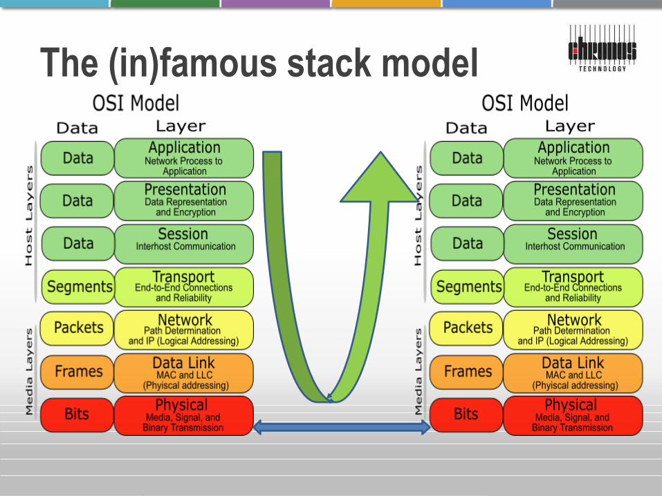
The (in)famous stack model

4

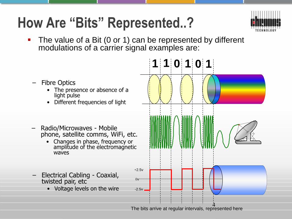
How Are “Bits” Represented..? The value of a Bit (0 or 1) can be represented by different

modulations of a carrier signal examples are:

1 1 1 0 1 0

– Fibre Optics • The presence or absence of a

light pulse • Different frequencies of light

The bits arrive at regular intervals, represented here

– Radio/Microwaves - Mobile phone, satellite comms, WiFi, etc.

• Changes in phase, frequency or amplitude of the electromagnetic waves

+2.5v

-2.5v

0v

– Electrical Cabling - Coaxial, twisted pair, etc

• Voltage levels on the wire

5

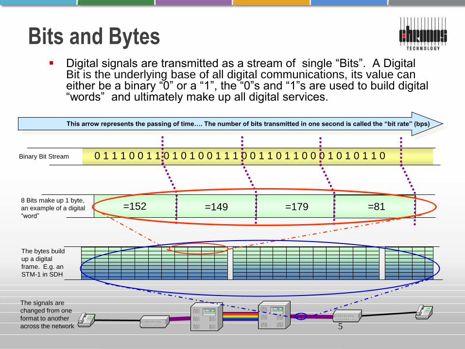
Bits and Bytes Digital signals are transmitted as a stream of single “Bits”. A Digital

Bit is the underlying base of all digital communications, its value can either be a binary “0” or a “1”, the “0”s and “1”s are used to build digital “words” and ultimately make up all digital services.

Binary Bit Stream

This arrow represents the passing of time…. The number of bits transmitted in one second is called the “bit rate” (bps)

0 1 1 1 0 0 1 1 0 1 0 1 0 0 1 1 1 0 0 1 1 0 1 1 0 0 0 1 0 1 0 1 1 0

8 Bits make up 1 byte,

an example of a digital

“word”

=149 =179 =81 =152

The bytes build

up a digital

frame. E.g. an

STM-1 in SDH

The signals are

changed from one

format to another

across the network

6

Timing (Frequency) Signal Characteristics

+

-

0

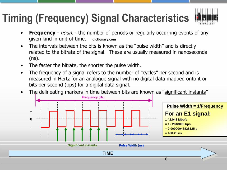
• Frequency - noun. - the number of periods or regularly occurring events of any given kind in unit of time. dictionary.com

• The intervals between the bits is known as the “pulse width” and is directly related to the bitrate of the signal. These are usually measured in nanoseconds (ns).

• The faster the bitrate, the shorter the pulse width.

• The frequency of a signal refers to the number of “cycles” per second and is measured in Hertz for an analogue signal with no digital data mapped onto it or bits per second (bps) for a digital data signal.

• The delineating markers in time between bits are known as “significant instants”

TIME

Significant instants Pulse Width (ns)

Frequency (Hz)

Pulse Width = 1/Frequency

For an E1 signal: 1 / 2.048 Mbp/s

= 1 / 2048000 bps

= 0.00000048828125 s

= 488.28 ns

7

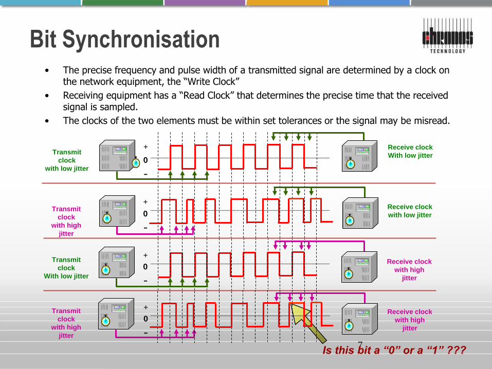
Bit Synchronisation • The precise frequency and pulse width of a transmitted signal are determined by a clock on

the network equipment, the “Write Clock”

• Receiving equipment has a “Read Clock” that determines the precise time that the received signal is sampled.

• The clocks of the two elements must be within set tolerances or the signal may be misread.

Is this bit a “0” or a “1” ???

+

-

0 Transmit

clock

with low jitter

Receive clock

With low jitter

+

-

0 Receive clock

with low jitter Transmit

clock

with high

jitter

+

-

0 Transmit

clock

With low jitter

Receive clock

with high

jitter

+

-

0 Receive clock

with high

jitter

Transmit

clock

with high

jitter

8

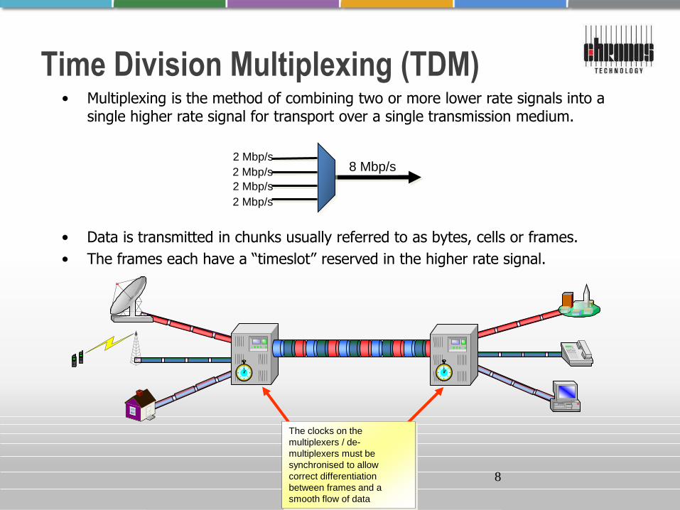
Time Division Multiplexing (TDM) • Multiplexing is the method of combining two or more lower rate signals into a

single higher rate signal for transport over a single transmission medium.

• Data is transmitted in chunks usually referred to as bytes, cells or frames.

• The frames each have a “timeslot” reserved in the higher rate signal.

8 Mbp/s 2 Mbp/s

2 Mbp/s

2 Mbp/s

2 Mbp/s

The clocks on the

multiplexers / de-

multiplexers must be

synchronised to allow

correct differentiation

between frames and a

smooth flow of data

9

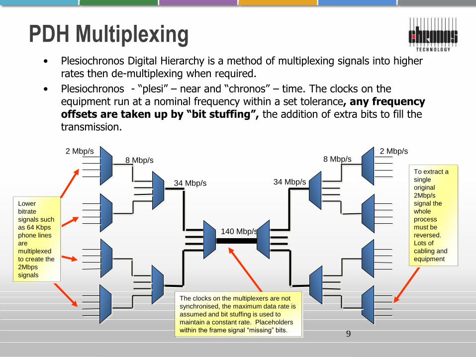
• Plesiochronos Digital Hierarchy is a method of multiplexing signals into higher rates then de-multiplexing when required.

• Plesiochronos - “plesi” – near and “chronos” – time. The clocks on the equipment run at a nominal frequency within a set tolerance, any frequency offsets are taken up by “bit stuffing”, the addition of extra bits to fill the transmission.

PDH Multiplexing

34 Mbp/s

8 Mbp/s 2 Mbp/s

140 Mbp/s

To extract a

single

original

2Mbp/s

signal the

whole

process

must be

reversed.

Lots of

cabling and

equipment

Lower

bitrate

signals such

as 64 Kbps

phone lines

are

multiplexed

to create the

2Mbps

signals

The clocks on the multiplexers are not

synchronised, the maximum data rate is

assumed and bit stuffing is used to

maintain a constant rate. Placeholders

within the frame signal “missing” bits.

34 Mbp/s

8 Mbp/s 2 Mbp/s

10

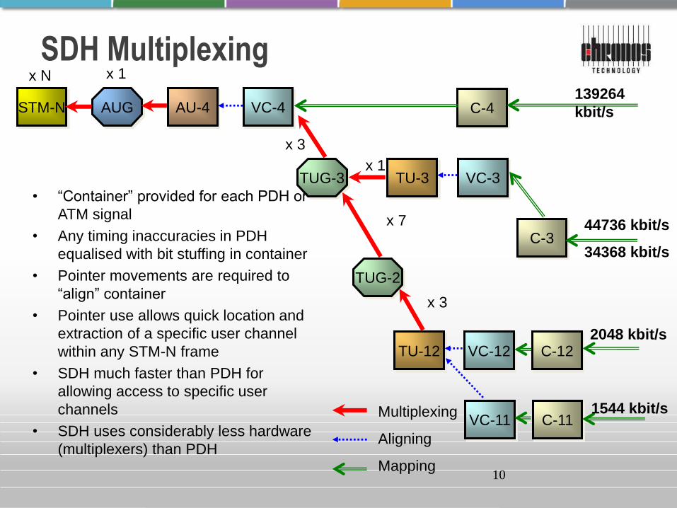
SDH Multiplexing

STM-N AUG AU-4

TUG-2

VC-4

TUG-3

C-4

TU-3 VC-3

C-3

TU-12 VC-12 C-12

VC-11 C-11 Multiplexing

Aligning

Mapping

x N x 1

x 3

x 1

x 7

x 3

139264

kbit/s

44736 kbit/s

34368 kbit/s

2048 kbit/s

1544 kbit/s

• “Container” provided for each PDH or

ATM signal

• Any timing inaccuracies in PDH

equalised with bit stuffing in container

• Pointer movements are required to

“align” container

• Pointer use allows quick location and

extraction of a specific user channel

within any STM-N frame

• SDH much faster than PDH for

allowing access to specific user

channels

• SDH uses considerably less hardware

(multiplexers) than PDH

11

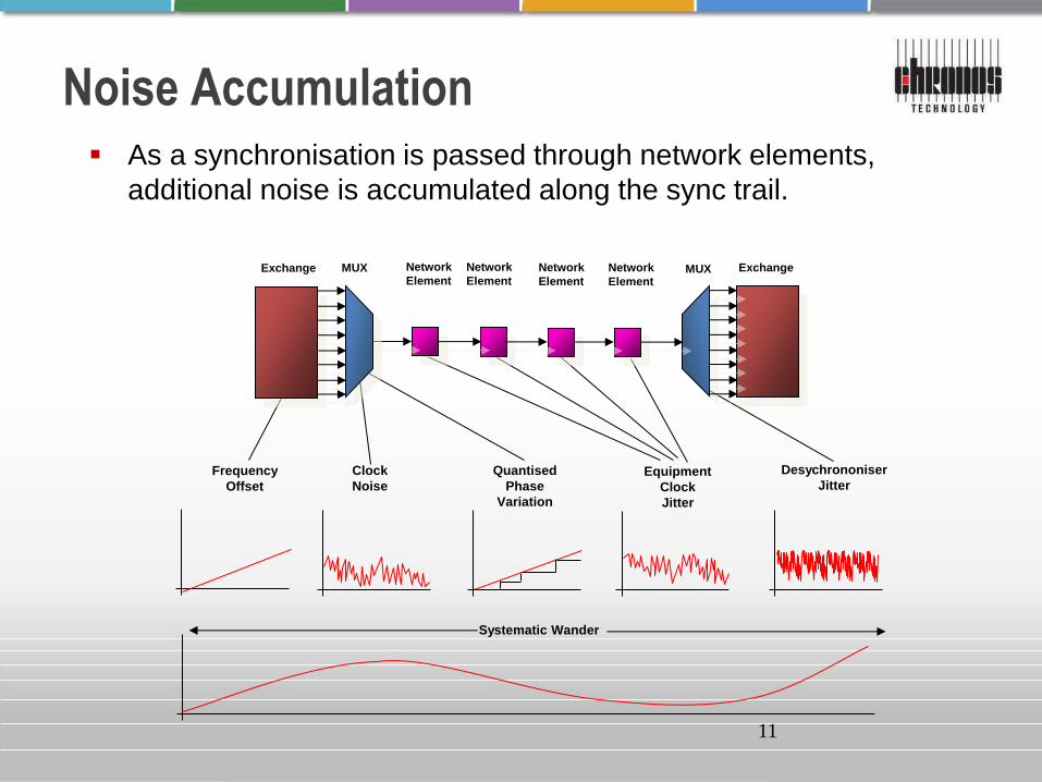
Noise Accumulation As a synchronisation is passed through network elements,

additional noise is accumulated along the sync trail.

Frequency

Offset

Clock

Noise

Quantised

Phase

Variation

Equipment

Clock

Jitter

Desychrononiser

Jitter

Systematic Wander

Exchange MUX Network

Element

Network

Element Network

Element

Network

Element

Exchange MUX

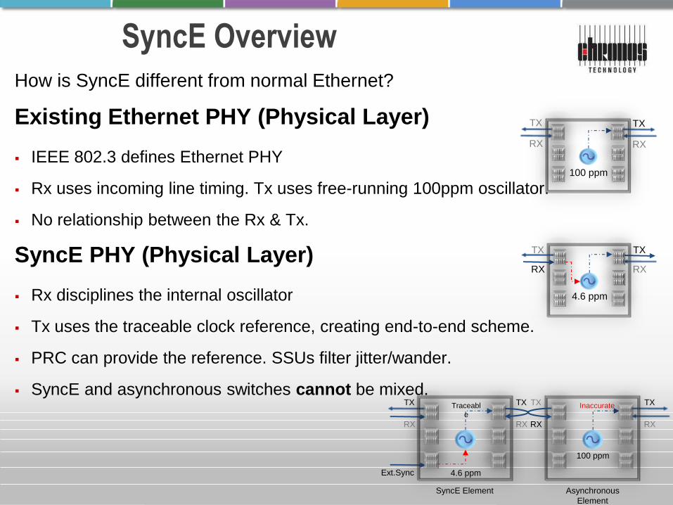
SyncE Overview How is SyncE different from normal Ethernet?

Existing Ethernet PHY (Physical Layer)

IEEE 802.3 defines Ethernet PHY

Rx uses incoming line timing. Tx uses free-running 100ppm oscillator.

No relationship between the Rx & Tx.

SyncE PHY (Physical Layer)

Rx disciplines the internal oscillator

Tx uses the traceable clock reference, creating end-to-end scheme.

PRC can provide the reference. SSUs filter jitter/wander.

SyncE and asynchronous switches cannot be mixed.

100 ppm

TX TX

RX RX

4.6 ppm

TX TX

RX RX

TX

RX

TX TX

RX RX

Ext.Sync

Inaccurate

100 ppm

4.6 ppm

TX

RX

Traceabl

e

SyncE Element Asynchronous

Element

13

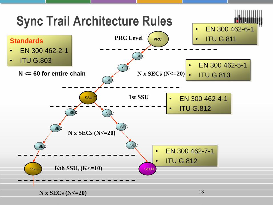
Sync Trail Architecture Rules

SSU-T Kth SSU, (K<=10)

SEC

SEC

SEC

N x SECs (N<=20)

N x SECs (N<=20)

Standards

• EN 300 462-2-1

• ITU G.803

PRC PRC Level

• EN 300 462-6-1

• ITU G.811

SSU-T 1st SSU • EN 300 462-4-1

• ITU G.812

SEC

SEC

SEC

N x SECs (N<=20)

• EN 300 462-5-1

• ITU G.813

• EN 300 462-7-1

• ITU G.812 SSU-L

SEC

SEC

SEC

N <= 60 for entire chain

14

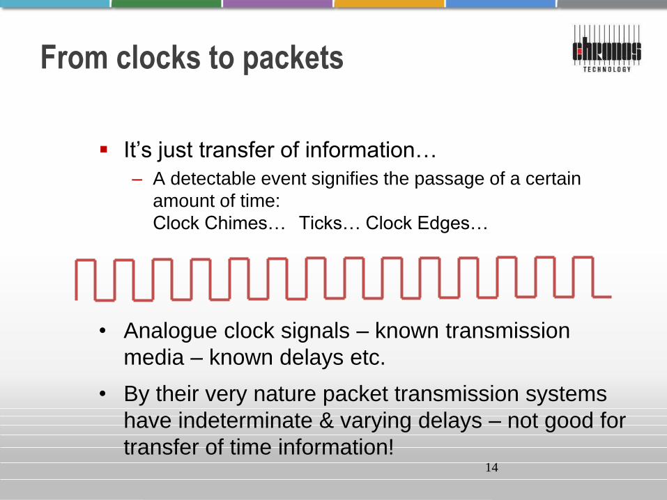
From clocks to packets

It’s just transfer of information…

– A detectable event signifies the passage of a certain

amount of time:

Clock Chimes… Ticks… Clock Edges…

• Analogue clock signals – known transmission

media – known delays etc.

• By their very nature packet transmission systems

have indeterminate & varying delays – not good for

transfer of time information!

15

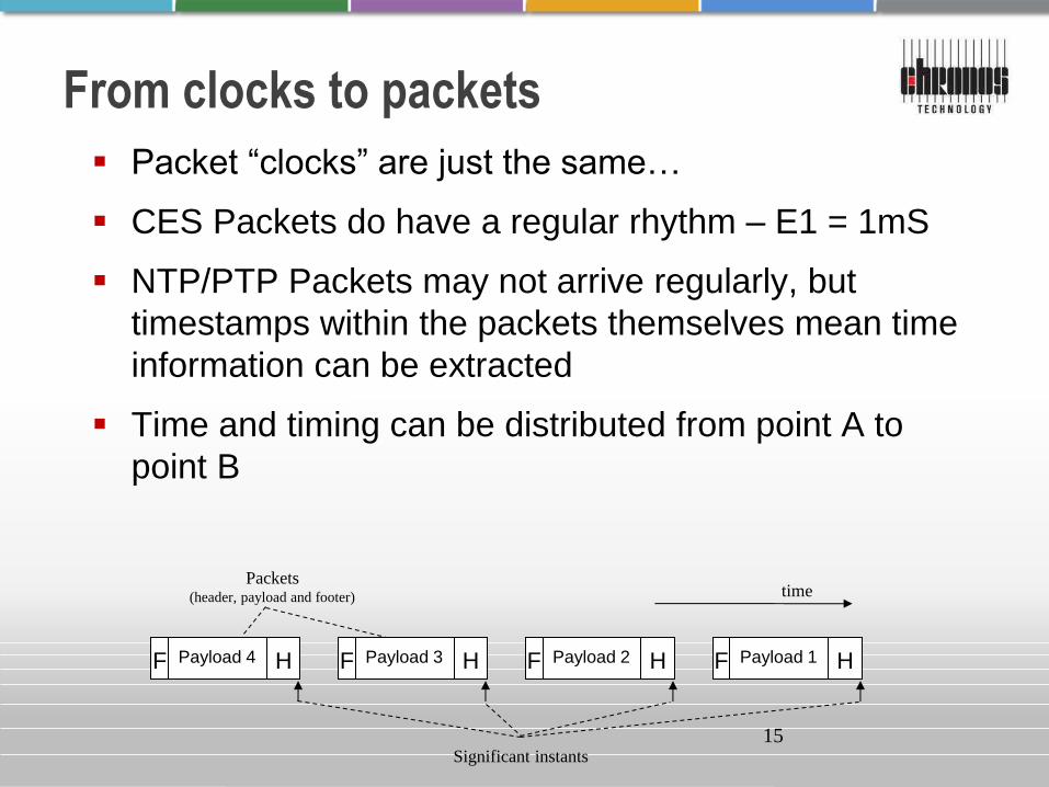
Packet “clocks” are just the same…

CES Packets do have a regular rhythm – E1 = 1mS

NTP/PTP Packets may not arrive regularly, but

timestamps within the packets themselves mean time

information can be extracted

Time and timing can be distributed from point A to

point B

Payload 4 H F Payload 2 H F Payload 3 H F Payload 1 H F

Packets (header, payload and footer) time

Significant instants

From clocks to packets

16

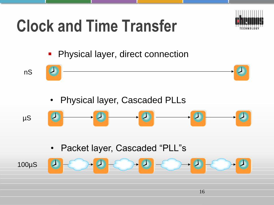
Clock and Time Transfer

Physical layer, direct connection

• Physical layer, Cascaded PLLs

• Packet layer, Cascaded “PLL”s

nS

µS

100µS

17

Packet Transport & Switching

Packet

Environment

FIFO Buffers

Voice

Video

Data

Voice

Video

Data

Main reason for problems with sync transport across an packet

environment is “Packet Delay Variation” and possible lost packets/

reordered packets

18

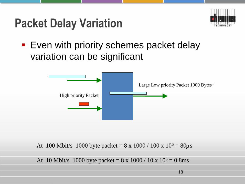
Packet Delay Variation

Even with priority schemes packet delay

variation can be significant

Large Low priority Packet 1000 Bytes+

High priority Packet

At 100 Mbit/s 1000 byte packet = 8 x 1000 / 100 x 106 = 80ms

At 10 Mbit/s 1000 byte packet = 8 x 1000 / 10 x 106 = 0.8ms

19

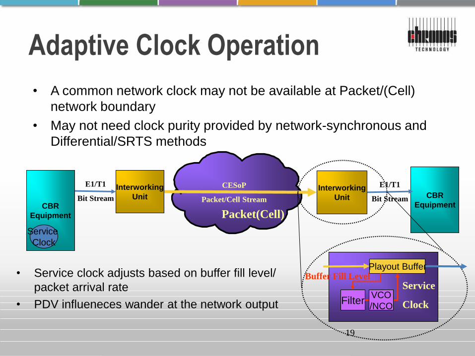
Packet(Cell)

Adaptive Clock Operation

Interworking

Unit

Interworking

Unit CBR

Equipment CBR

Equipment

E1/T1

Bit Stream

E1/T1

Bit Stream

CESoP

Packet/Cell Stream

• Service clock adjusts based on buffer fill level/

packet arrival rate

• PDV influeneces wander at the network output

Playout Buffer

Service

Clock Filter

Buffer Fill Level

• A common network clock may not be available at Packet/(Cell)

network boundary

• May not need clock purity provided by network-synchronous and

Differential/SRTS methods

Service

Clock

VCO

/NCO

20

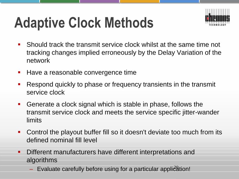
Adaptive Clock Methods

Should track the transmit service clock whilst at the same time not

tracking changes implied erroneously by the Delay Variation of the

network

Have a reasonable convergence time

Respond quickly to phase or frequency transients in the transmit

service clock

Generate a clock signal which is stable in phase, follows the

transmit service clock and meets the service specific jitter-wander

limits

Control the playout buffer fill so it doesn't deviate too much from its

defined nominal fill level

Different manufacturers have different interpretations and

algorithms

– Evaluate carefully before using for a particular application!

The adaptive method should be used only for wander insensitive

services

21

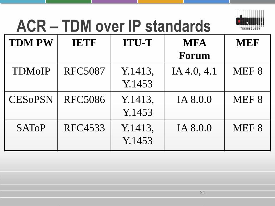
ACR – TDM over IP standards

TDM PW IETF ITU-T MFA

Forum

MEF

TDMoIP RFC5087 Y.1413,

Y.1453

IA 4.0, 4.1 MEF 8

CESoPSN RFC5086 Y.1413,

Y.1453

IA 8.0.0 MEF 8

SAToP RFC4533 Y.1413,

Y.1453

IA 8.0.0

MEF 8

22

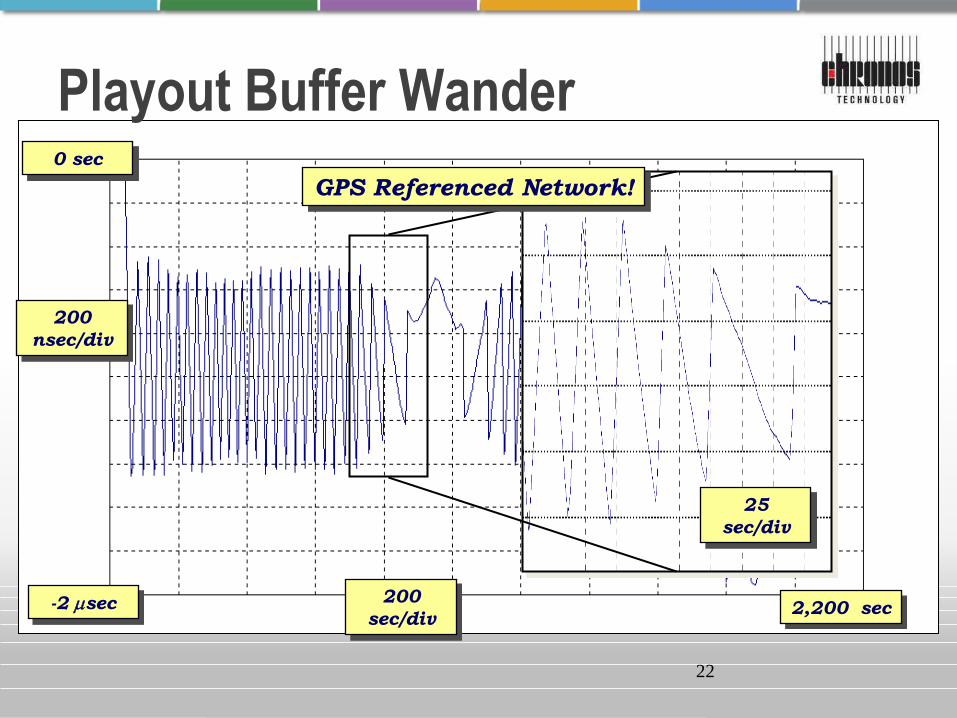
Playout Buffer Wander

-2 msec

0 sec

200

nsec/div

200

sec/div 2,200 sec

25

sec/div

GPS Referenced Network!

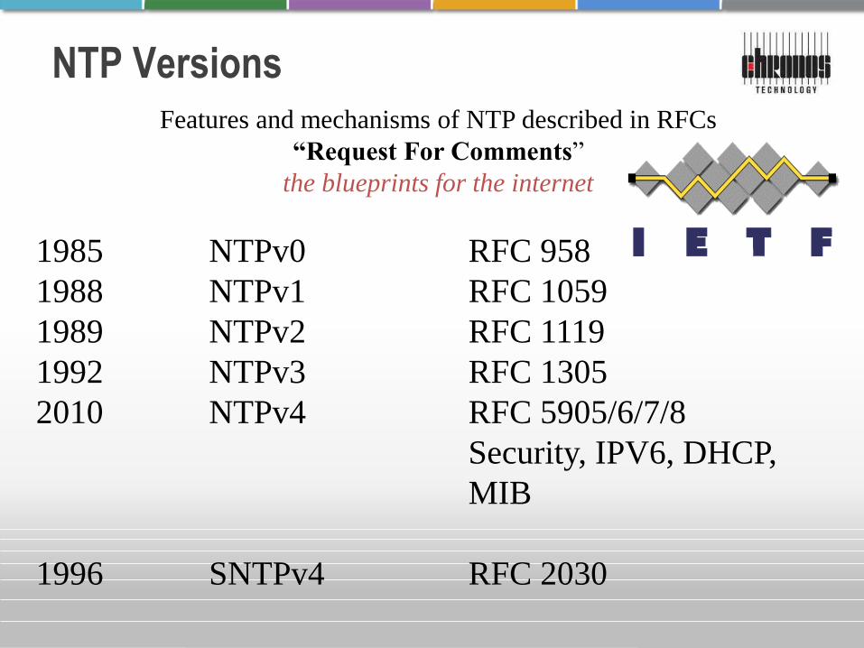
NTP Versions Features and mechanisms of NTP described in RFCs

“Request For Comments”

the blueprints for the internet

1985 NTPv0 RFC 958

1988 NTPv1 RFC 1059

1989 NTPv2 RFC 1119

1992 NTPv3 RFC 1305

2010 NTPv4 RFC 5905/6/7/8

Security, IPV6, DHCP,

MIB

1996 SNTPv4 RFC 2030

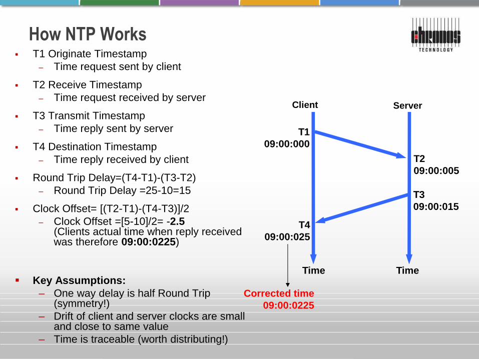
How NTP Works

T4

09:00:025

T3

09:00:015

T2

09:00:005

Client Server

T1

09:00:000

Time Time

Corrected time

09:00:0225

T1 Originate Timestamp

– Time request sent by client

T2 Receive Timestamp

– Time request received by server

T3 Transmit Timestamp

– Time reply sent by server

T4 Destination Timestamp

– Time reply received by client

Round Trip Delay=(T4-T1)-(T3-T2)

– Round Trip Delay =25-10=15

Clock Offset= [(T2-T1)-(T4-T3)]/2

– Clock Offset =[5-10]/2= -2.5 (Clients actual time when reply received was therefore 09:00:0225)

Key Assumptions:

– One way delay is half Round Trip (symmetry!)

– Drift of client and server clocks are small and close to same value

– Time is traceable (worth distributing!)

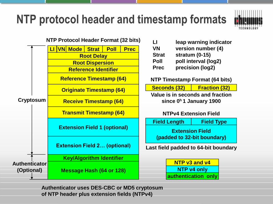
NTP protocol header and timestamp formats

Strat Poll LI Mode VN

NTP v3 and v4

Root Delay

Root Dispersion

Reference Identifier

Reference Timestamp (64)

Originate Timestamp (64)

Receive Timestamp (64)

Transmit Timestamp (64)

Message Hash (64 or 128)

NTP Protocol Header Format (32 bits) LI leap warning indicator

VN version number (4)

Strat stratum (0-15)

Poll poll interval (log2)

Prec precision (log2)

Seconds (32) Fraction (32)

NTP Timestamp Format (64 bits)

Value is in seconds and fraction

since 0h 1 January 1900

Authenticator uses DES-CBC or MD5 cryptosum

of NTP header plus extension fields (NTPv4)

Key/Algorithm Identifier

Cryptosum

Authenticator

(Optional)

Extension Field 1 (optional)

Extension Field 2… (optional)

NTP v4 only

Prec

Extension Field

(padded to 32-bit boundary)

Field Length Field Type

NTPv4 Extension Field

Last field padded to 64-bit boundary

authentication only

NTP Network Architecture

Satellite

Time Server

Router

Server Server

Router

Server Server Server

Router

Computer Computer ComputerComputerComputerComputerComputer

Stratum 1

Stratum 2

Stratum 3

GPS

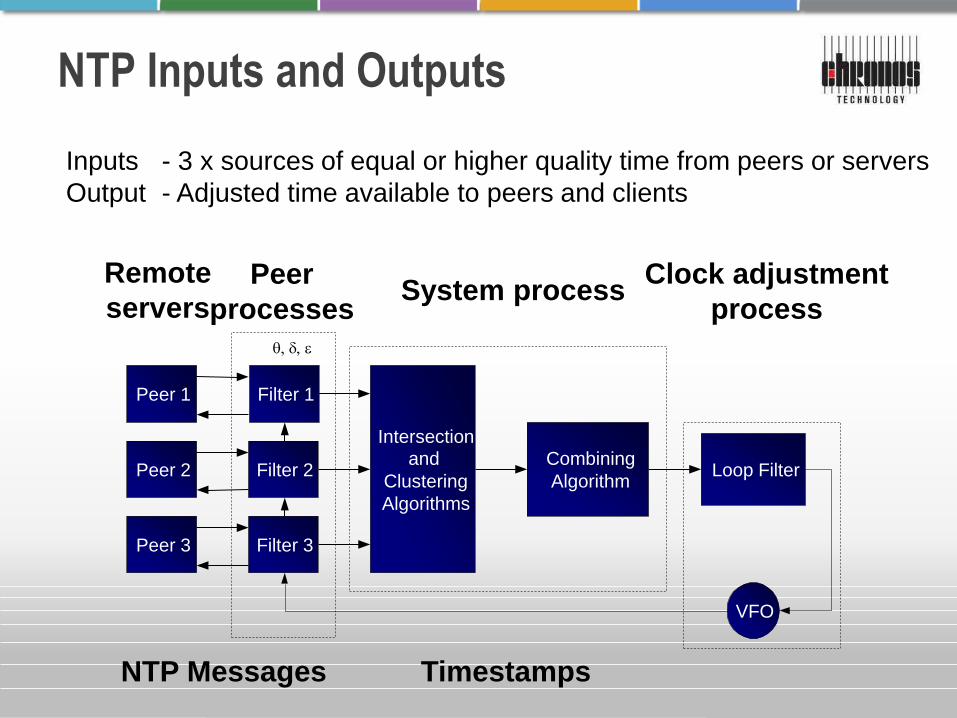
NTP Inputs and Outputs

Inputs - 3 x sources of equal or higher quality time from peers or servers

Output - Adjusted time available to peers and clients

Remote

servers Peer

processes System process

Clock adjustment

process

Peer 1

Peer 3

Peer 2

Filter 1

Filter 3

Filter 2

Intersection

and

Clustering

Algorithms

Combining

Algorithm Loop Filter

VFO

Timestamps NTP Messages

q, d, e

28

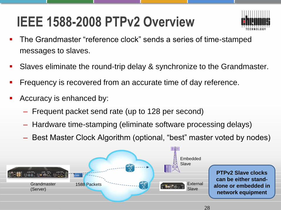
IEEE 1588-2008 PTPv2 Overview The Grandmaster “reference clock” sends a series of time-stamped

messages to slaves.

Slaves eliminate the round-trip delay & synchronize to the Grandmaster.

Frequency is recovered from an accurate time of day reference.

Accuracy is enhanced by:

– Frequent packet send rate (up to 128 per second)

– Hardware time-stamping (eliminate software processing delays)

– Best Master Clock Algorithm (optional, “best” master voted by nodes)

Grandmaster

(Server)

Embedded

Slave

External

Slave

1588 1588 1588

1588 Packets

1588 PTPv2 Slave clocks

can be either stand-

alone or embedded in

network equipment

29

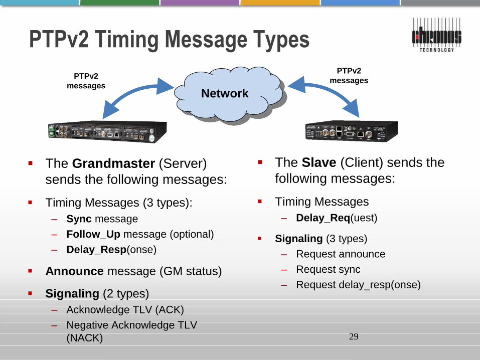
PTPv2 Timing Message Types

The Grandmaster (Server)

sends the following messages:

Timing Messages (3 types):

– Sync message

– Follow_Up message (optional)

– Delay_Resp(onse)

Announce message (GM status)

Signaling (2 types)

– Acknowledge TLV (ACK)

– Negative Acknowledge TLV

(NACK)

The Slave (Client) sends the

following messages:

Timing Messages

– Delay_Req(uest)

Signaling (3 types)

– Request announce

– Request sync

– Request delay_resp(onse)

Network

PTPv2

messages

PTPv2

messages

30

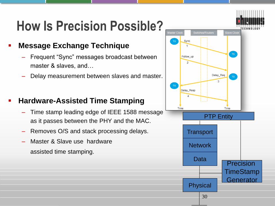
How Is Precision Possible?

Message Exchange Technique

– Frequent “Sync” messages broadcast between

master & slaves, and…

– Delay measurement between slaves and master.

Hardware-Assisted Time Stamping

– Time stamp leading edge of IEEE 1588 message

as it passes between the PHY and the MAC.

– Removes O/S and stack processing delays.

– Master & Slave use hardware

assisted time stamping.

Transport

Network

Data

Physical

PTP Entity

Precision

TimeStamp

Generator

31

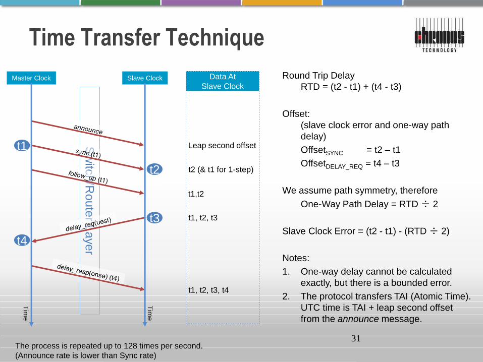
Time Transfer Technique

Master Clock Slave Clock

The process is repeated up to 128 times per second.

(Announce rate is lower than Sync rate)

Sw

itch/R

oute

r Layer

Tim

e

Tim

e

t2

t3

Data At

Slave Clock

Leap second offset

t2 (& t1 for 1-step)

t1,t2

t1, t2, t3

t1, t2, t3, t4

Round Trip Delay

RTD = (t2 - t1) + (t4 - t3)

Offset:

(slave clock error and one-way path

delay)

OffsetSYNC = t2 – t1

OffsetDELAY_REQ = t4 – t3

We assume path symmetry, therefore

One-Way Path Delay = RTD ÷ 2

Slave Clock Error = (t2 - t1) - (RTD ÷ 2)

Notes:

1. One-way delay cannot be calculated

exactly, but there is a bounded error.

2. The protocol transfers TAI (Atomic Time).

UTC time is TAI + leap second offset

from the announce message.

t1

t4

32

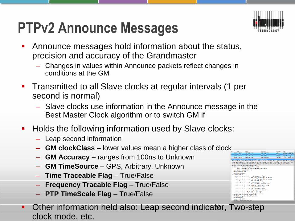
PTPv2 Announce Messages Announce messages hold information about the status,

precision and accuracy of the Grandmaster – Changes in values within Announce packets reflect changes in

conditions at the GM

Transmitted to all Slave clocks at regular intervals (1 per second is normal)

– Slave clocks use information in the Announce message in the Best Master Clock algorithm or to switch GM if

Holds the following information used by Slave clocks: – Leap second information

– GM clockClass – lower values mean a higher class of clock

– GM Accuracy – ranges from 100ns to Unknown

– GM TimeSource – GPS, Arbitrary, Unknown

– Time Traceable Flag – True/False

– Frequency Tracable Flag – True/False

– PTP TimeScale Flag – True/False

Other information held also: Leap second indicator, Two-step clock mode, etc.

33

PTPv2 Profiles

A profile is a subset of required options, prohibited options, and the

ranges and defaults of configurable attributes

– e.g. for Telecom: Update rate, unicast/multicast, etc.

– “The Telecom Profile” (G.8265.n/G.8275.n)

PTP profiles are created to allow organizations to specify selections of

attribute values and optional features of PTP that, when using the

same transport protocol, inter-works and achieve a performance that

meets the requirements of a particular application

Other (non-Telecom) profiles:

– IEEE C37.238-2011 Power Distribution Industry “Smart grid”

– 802.11AS AV bridging (e.g. AV over domestic LAN)

34

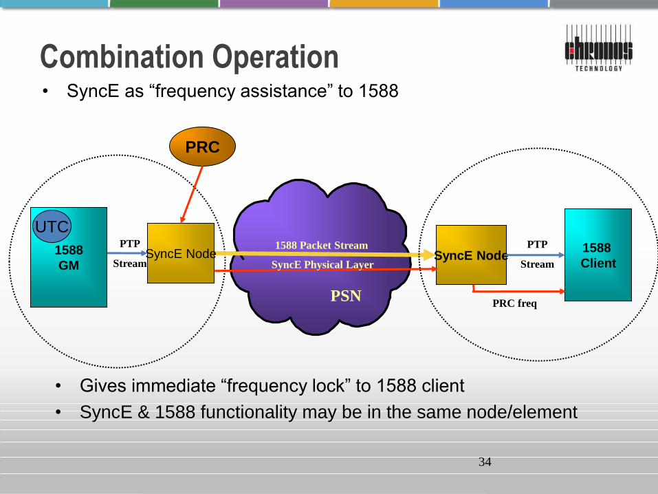
PSN

Combination Operation

SyncE Node SyncE Node 1588

Client 1588

GM

PTP

Stream

PTP

Stream

1588 Packet Stream

• SyncE as “frequency assistance” to 1588

UTC

PRC

SyncE Physical Layer

PRC freq

• Gives immediate “frequency lock” to 1588 client

• SyncE & 1588 functionality may be in the same node/element

Summary

Physical Layer Sync Distribution

– Historically frequency, phase

Packet Layer Sync Distribution

– Historically time (NTP)

– PTP (& “carrier class” NTP) add frequency & phase

Combination operation

– Using both physical and packet layers to deliver

frequency, phase & time with greater accuracy &

reliability.

www.chronos.co.uk

www.syncwatch.com

Christian.Farrow@chronos.co.uk

Thankyou

Questions?