two blades of grass: the impact of the green revolution

NBER WORKING PAPER SERIES

TWO BLADES OF GRASS:THE IMPACT OF THE GREEN REVOLUTION

Douglas GollinCasper Worm Hansen

Asger Wingender

Working Paper 24744http://www.nber.org/papers/w24744

NATIONAL BUREAU OF ECONOMIC RESEARCH1050 Massachusetts Avenue

Cambridge, MA 02138June 2018

We would like to thank Philipp Ager, Felipe Valencia Caicedo, Carl-Johan Dalgaard, Stefan Dercon,Dave Donaldson, Cheryl Doss, James Fenske, Nicola Gennaioli, Walker Hanlon, Peter Sandholt Jensen,Nicolai Kaarsen, Tim Kelley, Nathan Nunn, James Stevenson, David N. Weil, and seminar participantsat the University of Copenhagen, McGill, the 7th Annual Workshop on Growth, History and Developmentat the University of Southern Denmark, the 2016 annual European Economic Association meetingin Geneva, the 2017 annual AEA meeting in Chicago, and the NBER conference on Trade and Agriculturefor helpful comments and suggestions. Douglas Gollin currently serves as chair of the Standing Panelon Impact Assessment (SPIA) of the Independent Science and Partnership Council (ISPC) of the CGIAR,the publicly funded agricultural research and development consortium under whose auspices manyof the Green Revolution varieties were developed. Gollin's views do not represent those of SPIA, theISPC, or the CGIAR. The views expressed herein are those of the authors and do not necessarily reflectthe views of the National Bureau of Economic Research.

NBER working papers are circulated for discussion and comment purposes. They have not been peer-reviewed or been subject to the review by the NBER Board of Directors that accompanies officialNBER publications.

© 2018 by Douglas Gollin, Casper Worm Hansen, and Asger Wingender. All rights reserved. Shortsections of text, not to exceed two paragraphs, may be quoted without explicit permission providedthat full credit, including © notice, is given to the source.

Two Blades of Grass: The Impact of the Green RevolutionDouglas Gollin, Casper Worm Hansen, and Asger WingenderNBER Working Paper No. 24744June 2018JEL No. N50,O11,O13,O50,Q16

ABSTRACT

We examine the economic impact of high-yielding crop varieties (HYVs) in developing countries 1960-2000. We use time variation in the development and diffusion of HYVs of 10 major crops, spatial variation in agro-climatically suitability for growing them, and a differences-in-differences strategy to identify the causal effects of adoption. In a sample of 84 counties, we estimate that a 10 percentage points increase in HYV adoption increases GDP per capita by about 15 percent. This effect is fully accounted for by the direct effect on crop yields, factor adjustment, and structural transformation. We also find that HYV adoption reduced both fertility and mortality.

An online appendix is available at: http://www.nber.org/data-appendix/w24744

Douglas GollinUniversity of OxfordDepartment of International Development Queen Elizabeth House3 Mansfield RoadOxford OX1 3TBUnited [email protected]

Casper Worm HansenUniversity of CopenhagenØster Farimagsgade 5Copenhagen, [email protected]

Asger WingenderDepartment of EconomicsUniversity of CopenhagenOester Farimagsgade 5, building 26DK-1353 Copenhagen [email protected]

“Whoever makes two ears of corn, or two blades of grass, to grow

upon a spot of ground where only one grew before, would deserve

better of mankind, and do more essential service to his country,

than the whole race of politicians put together.”

Jonathan Swift in Gulliver’s Travels

1 Introduction

How important is agricultural productivity growth in development? Early views of development

assumed that most of the impetus for development and economic growth would necessarily come from

the industrial sector, which was thought to offer the potential for rapid rates of productivity growth. In

contrast, the agricultural sector in most developing countries was seen as backward and stagnant, with

limited potential for growth (e.g., Lewis (1951)). In recent years, agriculture’s potential significance

has been a theme in a renewed literature on structural transformation and growth. A new literature

has offered theoretical models in which agricultural productivity growth may prove important for

subsequent industrialization and in which agricultural productivity differences may play a role in

explaining cross-country disparities in income.1 However, it has proved difficult to assess the overall

importance of agriculture’s contributions to growth, and a lively policy debate remains on whether

(and when, where, and how) governments should focus their development efforts on agriculture.

This paper takes advantage of new data sources that make it possible to examine the impacts of

what is arguably the most important episode of agricultural innovation in modern history – the Green

Revolution that began in the 1960s. As Evenson and Gollin (2003a) argued, the Green Revolution

is best understood as an increase in the rate of growth of agricultural productivity, based on the

application of modern crop breeding techniques to the agricultural challenges of the developing world.

The Green Revolution emerged from philanthropic efforts – arguably shaped by geopolitical interests

– to address the challenges of rural poverty and agrarian unrest in the late 1950s and early 1960s,

and it involved a concerted effort to apply scientific understandings of genetics to the development of

improved crop varieties that were suited to the growing conditions of the developing world. The Green

Revolution delivered a massive and nearly immediate impact in some locations in the developing world

1See, for example, Caselli and Coleman (2001); Caselli (2005); Cordoba and Ripoll (2009); Gollin et al. (2002, 2007);Restuccia et al. (2008); Vollrath (2011). However, as stressed by Matsuyama (1992), from a basic theoretical perspective,the relationship between agricultural productivity and economic growth is ambiguous, depending on whether economiesare open or closed, and so in that sense it is not ex-ante obvious how the adoption HYVs should influence economicgrowth, which ultimately makes it an empirical question.

2

– particularly in the irrigated rice-growing areas of Asia and the wheat-growing heartlands of Asia

and Latin America. These were the focal points for the greatest initial research efforts, and they were

also the easiest places in which to develop widely adapted new varieties. Other parts of the developing

world received little benefit, however, from these early efforts – for reasons that will be discussed in

detail below.

How much did the Green Revolution matter? Did the agricultural productivity increases generate

large and long-lasting benefits? Answering this question has been difficult, because of the obvious

challenges to causal identification. Because growth in one sector of an economy will inevitably link

(positively and/or negatively) to growth in other sectors, it is challenging to find compelling evidence at

the national level for the causal impacts of agricultural productivity growth. There is more evidence –

and more convincing evidence – of such impacts at the micro level or at the regional level. Several recent

papers have made use of quasi-natural experiments (e.g., Bustos et al. (2016) and Hornbeck and Keskin

(2011)) or structural estimation (e.g., Foster and Rosenzweig (2004), Foster and Rosenzweig (2007))

to look at the cross-sectoral impacts of shocks to agricultural productivity. However, these localized

effects can be difficult to generalize to full general equilibrium impacts on aggregate economies. The

local movements of people across sectors are only a relatively small part of the transformation process.

In particular, for poor countries with large fractions of their workers initially in agriculture, the main

mechanisms of structural transformation are not played out within local labor markets. Instead, they

involve large-scale movements of people across locations – from rural to urban or from one region

to another. Studies that emphasize the local movements of people will miss these broader and more

secular changes.

This paper models the impact of the Green Revolution on national economies, rather than on

local labor markets. The main idea is to use exogenous variation in geography, combined with the

essentially exogenous (to individual countries) timing of agricultural research successes in a differences-

in-differences strategy, to instrument for the timing and magnitude of agricultural productivity shocks

received by countries. This allows us to trace the impact of agricultural productivity increases across

a large set of countries. We observe strong and robust impacts of these Green Revolution productivity

shocks. Most striking is the impact on per capita GDP. Depending on the specification, we find that

a 10-percentage point increase in the share of area under high-yielding varieties (HYVs) in 2000 is

associated with a 10-15 percentage point increase in per capita GDP. Moreover, we find no evidence

that the Green Revolution was offset substantially by Malthusian effects; the increased availability of

food was not eroded by population increases. Instead, population appears to have declined, if anything,

3

in response to the growth in agricultural productivity. Our paper also sheds light on a concern often

expressed in the literature about the potential for agricultural productivity improvements to pull

additional land into agriculture at the expense of forests and other environmentally valuable land

uses. We find that, to the contrary, increases in the area under HYV has tended to reduce the amount

of land devoted to agriculture – consistent with what has been termed the “Borlaug hypothesis.” Under

this hypothesis, improvements in the productivity of food crops leads to intensification of agriculture

on a smaller land area, preventing expansion on the extensive margin.2

We further show that the impact of the Green Revolution on per capita GDP comes from effects on

total factor productivity (TFP) beyond those simply derived from increases in crop yields – including,

for instance, changes in the quality of land, fertilizer use, labor, and capital. Our analysis also finds

that per capita GDP rises due to factor adjustments of various kinds. Likewise, we can look at the

channels through which the Green Revolution appears to have altered population size. Our analysis

suggests that the main effect occurs through an effect of the Green Revolution on lower birthrates. In

the data, this effect is only partly offset by an increase in life expectancy; the net result is a negative

effect on population growth.

A large literature considers the social, economic, and environmental impacts of the Green Rev-

olution; it would be too ambitious to review this literature here. Recent surveys in the economics

literature include Renkow and Byerlee (2010) and Pingali (2012). Our paper addresses some of the

same macro-scale questions that have previously been considered using different methods by Evenson

and Rosegrant (2003), Perez and Rosegrant (2015), and others. These studies have used a range of

models of varying structures and with differing assumptions. A recent survey of these models can

be found in Godfray and Robinson (2015). In contrast to these approaches, our analysis is based

on econometric evidence from a panel of countries. As noted above, our identification approach uses

agroecological variation combined with time variation arising from the Green Revolution as an in-

strument for technology change. This type of empirical strategy has been used previously to look

at the effects of the adoption of potatoes in Europe following the Columbian Exchange (Nunn and

Qian (2011a)), and the impact of agricultural productivity improvements on local economic develop-

ment (Bustos et al. (2016)), for example. Other studies that have been exploiting the agroecology

2Norman Borlaug (1914-2009) was a wheat scientist closely associated with the early years of the Green Revolution.Borlaug won the Nobel Peace Prize in 1970 for his work in developing and promoting the Green Revolution, most notablythrough his efforts in wheat breeding for yield and rust resistance. Borlaug argued forcefully that improved varietiesand higher agricultural productivity would lead to reduced pressure on land resources, as higher production would beachieved through intensification rather than extensive expansion of agricultural area. This argument was dubbed the“Borlaugh hypothesis” by Angelsen et al. (2001), p. 3.

4

component directly include, Easterly (2007), who looks at the impact of plantation agriculture on long-

run development patterns, and Bentzen et al. (forthcoming) who investigate the impact of irrigated

agriculture on political outcomes. This paper is also related to an even larger literature which has

considered the impact of agricultural science or research on economic and social outcomes at a more

geographically limited scale. This literature has been surveyed by Maredia and Byerlee (2000); other

important contributions include Fan et al. (2002); Meinzen-Dick et al. (2003); Thirtle et al. (2003);

Pingali and Kelley (2007); Dalrymple (2008); Raitzer and Kelley (2008); Rusike et al. (2010).

In the remainder of this paper, we begin in Section 2 by documenting the historical context in which

the Green Revolution unfolded, including the institutional background for the scientific research that

gave rise to the Green Revolution. Section 3 presents data on the diffusion of HYV crops that were

at the core of the Green Revolution. Section 4 describes the estimation strategy, including a detailed

discussion of our identifying assumptions. Section 5 presents our estimates of the long-term and large-

scale consequences of the Green Revolution. In Section 6, we explore the potential channels for these

impacts; Section 7 concludes with implications for long-term strategies of growth and development.

2 Background: The Green Revolution

Although formal programs of scientific research on crop improvement in developing countries can be

traced back into the nineteenth century and before, the Green Revolution of the 20th century can be

dated fairly precisely. Following some early exploratory work in the 1940s and 1950s, the major efforts

can be traced to the creation in 1960 of the International Rice Research Institute (IRRI), located near

the town of Los Banos in the Philippines, and in 1967 of a sister institution, the International Center

for Maize and Wheat Improvement (CIMMYT), with headquarters near Texcoco, Mexico. These two

research centers were funded by a group of aid donors, including the Ford and Rockefeller Foundations

as well as a number of national aid agencies. CIMMYT grew out of an ongoing program of wheat

research that the Rockefeller Foundation had been funding in Mexico since the late 1940s, under the

leadership of Norman Borlaug, a plant pathologist and wheat breeder who went on to win the Nobel

Peace Prize in 1970 for his efforts. The history of the early Green Revolution has been documented

previously in a number of sources, e.g., Dalrymple et al. (1974); Dalrymple (1978, 1985, 1986); Barker

et al. (1985). Breeding efforts at these institutions were subsequently extended to other crops and

other research centers, as discussed below.

For the purposes of this paper, it is important that the timing of the initial Green Revolution and

5

its subsequent patterns of diffusion were largely exogenous to individual countries. The argument we

will make is based on two claims. The first is that the timing of the initial research was driven by a

mixture of humanitarian and geopolitical concerns and coincided with the birth of the international

aid community; in this sense, it was not driven by an assessment of the subsequent growth prospects

of any particular country or set of countries. The second is that the principal initial research behind

the Green Revolution in rice and wheat diffused rapidly from the locations where the research was

initially carried out. Diffusion took place very rapidly in similar agroecological areas and more slowly

in areas with less favorable geographies. The research targeted particular agronomic and phenotypic

problems thought to have widespread relevance, rather than focusing on specific countries. And in

spite of the rapid success of research on rice and wheat, it took much longer for the Green Revolution

to be extended to other crops, reflecting large differences in the initial stock of scientific knowledge as

well as the greater heterogeneity of growing environments. On all counts, we argue that the differential

impact of agricultural research on developing economies reflected factors substantially exogenous to

those countries.

2.1 The Timing of the Green Revolution

The start of the Green Revolution can be defined quite precisely. Although many developing countries

had some indigenous and colonial programs of crop improvement, it is a reasonable generalization to

say that few developing countries had large or systematic programs of crop improvement before 1950.

Colonial programs of agricultural research tended to focus on non-food crops, such as sugar, that

provided raw materials for industry or were consumed in the colonial heartland. Food crops tended

to receive a low priority. To the extent that there were active programs of research on food crops, as

in India, in the first half of the twentieth century, they tended to focus on identifying vigorous strains

of existing varieties rather than developing new lines. According to De Datta (1981), rice research

in the developing world in the early 20th century tended to consist of little more than selection of

high-performing varieties from farmers’ fields, along with some efforts to introduce materials from

other geographies and to select them for local adaptation. Very little cross-fertilization was attempted

– essentially the effort to create new genetic mixes through deliberate breeding of one variety to

another – because of the relative technical difficulty of this process and perhaps also because of the

limited familiarity with the principles of Mendelian genetics that are required to make sense of cross-

6

fertilization.3

For rice and wheat, the first large-scale programs of cross-fertilization (henceforth, “breeding”)

were those carried out by IRRI and CIMMYT (including the precursor Rockefeller program on wheat

in Mexico), beginning in the 1950s and early 1960s.4 In both crops, these early efforts reflected an

emerging view that rich countries had both obligations and opportunities to encourage development in

the newly independent countries of Africa and Asia, in the wake of the Second World War. This view

coincided with geostrategic concerns triggered by the Cold War. The threat of agrarian revolutions

in Asia and Latin America seemed to call for efforts to promote rural development – and in turn to

focus on agricultural productivity (for a detailed discussion, see Perkins (1997)). It was presumably

not a coincidence that the United States, being pulled steadily into a war in Indochina and fearing

a domino effect, chose to support investments in rice research; nor that it would support a wheat

research program that was based in Mexico.

Against this backdrop, rice breeding began at IRRI in 1965, several years after the founding of the

institute, and within the first weeks of breeding effort, scientists made a cross that gave rise to what

would eventually prove to be the first “mega-variety” of rice. For wheat, it is similarly possible to

identify a zero-date for the Green Revolution: the first successful crosses from the Rockefeller wheat

program took place in 1955, and the first varieties were released in Mexico in 1961.

The sections below will describe the diffusion of HYVs of rice, wheat, and other crops. A key

point is that the diffusion patterns were initially shaped largely by the extent of research effort and

by agroecological similarity to the locations where the initial research was carried out. Diffusion of

high-yielding rice and wheat to less favorable areas was more gradual and reflected the time required to

address different geographies and agronomic problems of narrower significance. Similarly, the eventual

development and spread of HYVs of maize, sorghum, millet, root crops, and legumes was driven in

significant measure by the timing and scale of the international research efforts. These efforts can be

3Rice and wheat are self-pollinating crops in which each small flower on a stalk tends to pollinate itself. Cross-fertilization is a painstaking process that (in the 1960s) required emasculating certain stalks by carefully removing themale portion of the flower with a tweezers so that it will be unable to pollinate itself and can then be pollinated fromanother source chosen by the scientist. This contrasts with the relative ease of cross-fertilization (hybridization) in maize,where the tassels growing at the top of the plant are the male flowers and can be removed very simply by “de-tasseling”a row of plants.An understanding of genetics is important for cross-fertilization programs because the first generation offspring of a crosswill typically display considerable heterogeneity, with different traits expressed in predictable ratios. An inexperiencedbreeder may not be able effectively to identify desirable offspring; these must in turn be selected and reselected throughfive or six generations before they display sufficient uniformity to be acceptable to farmers.

4IRRI too had a modest precursor program, a small breeding effort initiated under the auspices of the UN Food andAgriculture Organization (FAO) in the 1940s and 1950s. It is safe to say, however, that there was no large-scale orsystematic effort to breed new rice varieties for the developing world before 1960.

7

identified in large degree with the creation of new research centers and programs. Thus, in the wake

of the successes of IRRI and CIMMYT, two additional centers were created in 1967, the International

Institute for Tropical Agriculture (IITA) in Ibadan, Nigeria, and the International Center for Tropical

Agriculture (CIAT) in Cali, Colombia. These institutions were assigned mandates for additional crops

and different agroecologies; the subsequent rolling out of additional centers provides a valuable tool

for identification in our analysis. There are now fifteen such institutions that carry out agricultural

research on subjects ranging from aquaculture to livestock science to climate adaptation.5

To a degree, adaptive breeding – the effort to tailor HYVs to specific agroecological niches and

to address problems of local importance – has been carried out by national governments through

agricultural research systems, university-based research programs, and other local research. A concern

for our identification strategy is that this effort may thereby reflect institutional capacity, raising the

possibility that the diffusion curves for different countries are related to general institutional factors

that might lead to growth through other channels. But what is clear is that even for the most advanced

developing countries, adaptive breeding has continued even to the present day to rely heavily on

research emerging from the CGIAR. Many or most HYV crops in the developing world continue to

use genetic material that can be traced to the CGIAR, and almost all national research programs in

the developing world maintain close connections to CGIAR institutions. In that sense, the research

products of the CGIAR continue to play a significant role in shaping the diffusion of HYVs. The

role of the CGIAR and of international research institutions through the late 1990s is documented

fully in Evenson and Gollin (2003b); a more recent study by Walker and Alwang (2015) describes the

continuing importance of international research for the diffusion of HYVs in sub-Saharan Africa.6

Beyond the institutional role of the CGIAR in the development of HYVs, an additional source of

exogeneity is the sheer difficulty of achieving research success in different crops. The rapid progress of

varietal improvement in rice and wheat for favorable environments turned out to be a happy accident.

As discussed below, it turned out that in both crops, substantial yield gains could be achieved through

the introduction of a single gene for dwarfism. But an additional underlying reason for the rapid

successes in these crops was that research built on a large stock of scientific knowledge. Both crops

had been heavily researched prior to the 1960s in advanced countries, and scientists could work with

5These centers operate collectively as an entity known as the CGIAR (formerly known as the Consultative Group onInternational Agricultural Research). CGIAR defines itself today as a “worldwide partnership addressing agriculturalresearch for development.” Its research is funded by national and multilateral development agencies, non-governmentalorganizations, private philanthropies, and other donors, with an annual budget approaching $1 billion in 2015.

6A chapter (Pandey et al. (2015)) in the book also by Walker and Alwang (2015) discusses international researchimpacts in recent times in South Asia.

8

elite breeding lines. Moreover, they had a good understanding of the extent of genetic diversity and

the sources of useful genes. The situation was very different for tropical root crops such as cassava and

sweet potato; it was also quite different for crops that were relatively minor in rich countries, such as

millet and sorghum. These differing initial stocks of knowledge and improved genetic materials create

another source of exogenous variation in the timing and extent of the Green Revolution. Evenson and

Gollin (2003a) argued that the slow diffusion of HYVs in sub-Saharan Africa reflected the differences

in crop mix and agroecology relative to Asia. Because crop varieties can be highly location specific,

there were limited spillovers of crop varieties from Asia to Africa. The Green Revolution varieties of

rice proved poorly suited to Africa; maize varieties that had performed well in Mexico also proved

disappointing under farmers’ conditions in Africa.

2.2 History of the Green Revolution in Rice

This section considers the detailed case of the Green Revolution in rice in South and Southeast Asia.

We argue here that genetic and agroecologic factors created a strong element of exogeneity to the

diffusion of HYVs of rice.

As noted by ?, varietal improvement efforts in rice and wheat can be dated well back into the 19th

century and beyond; but the distinctive feature of the early Green Revolution was the development and

introduction of short semi-dwarf varieties of rice and wheat that were adapted to tropical and semi-

tropical environments. These short varieties were well suited to intensive cultivation. In particular,

they responded well to heavy doses of fertilizer. For both rice and wheat, traditional varieties tended

to be substantially taller; it was not uncommon for tropical Asian rice varieties to be two meters

tall, whereas the semidwarfs were closer to one meter tall. The taller varieties suffered from two

disadvantages. First, a large amount of the plant’s energy was devoted to the production of leaves and

stalks, with a relatively small fraction of the plant biomass being allocated to grain. Second, the tall

varieties were subject to an architectural design flaw; since grain grows near the top of a rice plant or

wheat plant, heavy grain yields would make the plants top-heavy and would induce them to fall over

– a problem known as “lodging.” For rice, Barker et al. (1985) note that lodging was a constraint on

crop yields in tropical Asia: “Particularly in the irrigated areas, fields of lodged rice (with stalks bent

over and panicles lying flat on the ground) were a familiar sight at harvest-time. Fertilizer was not

used because the application of nitrogen to tall indica varieties weakened the stalks, advancing the

date of lodging and further reducing yields” (Barker et al. (1985)).

The architecture of rice and wheat plants thus implied that chemical fertilizers were little used

9

in tropical production of these crops through the 1950s. As reported by Barker et al. (1985) (Table

6.2, p. 77), NPK fertilizer use on rice in India in the 1956-60 period was approximately 2 kg/ha,

compared with over 200 kg/ha in Japan or Taiwan. Essentially zero fertilizer was used on rice in

Bangladesh, Indonesia, Thailand, or other countries in the global heartland of rice cultivation. Crop

yields were correspondingly low, as plants were starved for nutrients: in 1965, Indian rice yields were

1.3 t/ha, and similarly low levels prevailed in Cambodia (1.1 t/ha), Indonesia (1.8 t/ha), Bangladesh

(1.7 t/ha), Pakistan (1.4 t/ha), and the Philippines (1.3 t/ha). By contrast, in northern Asia and in

rich countries, yields were commonly 4.5-6.5 t/ha (FAOSTAT).

The rice and wheat scientists involved in forming the nascent IRRI and CIMMYT were clear that

one of their first research challenges was to develop shorter varieties of these crops, with stiffer straw,

that would tolerate more intensive use of fertilizer. They also sought shorter duration varieties with

broad adaptability to different environments. Short varieties of rice and wheat were known and had

been cultivated in northern Asia, possibly for many centuries, although ? writes that the agronomic

potential of these varieties did not become clear until the 20th century and the advent of chemical

fertilizers. These varieties were not well suited to tropical and semi-tropical conditions, however. As a

result, the earliest breeding efforts at IRRI involved focusing on crosses of these semi-dwarf varieties

with sturdy and well adapted tropical rice varieties. The eighth cross made, in the first weeks of IRRI’s

existence, was of an Indonesian variety (Peta) with a semi-dwarf from Taiwan (Dee-Geo-Woo-Gen, or

DGWG). The resulting cross, known as IR8, was arguably one of the most successful innovations in

human history. IRRI released seed of IR8 in 1965, and by 1969 approximately 10 percent of Asia’s

rice area was planted in IR8 or other varieties, most of them derived from IR8 or closely related to

it (Herdt and Capule (1983)). By 1980, about 16 million ha, accounting for around 40 percent of

Asia’s rice area, was planted in what became known as high-yielding rice varieties, as estimated by

Dalrymple (1986).

Diffusion HYVs of rice was extraordinarily rapid in those areas where the varieties were well

adapted. Although at the micro level, adoption was associated with a variety of individual farmer

characteristics such as education, land tenure, and farm size, the aggregate patterns suggested very

large disparities within and across countries based on agroclimatic and agroecological factors. The

reliable availability and controlled supply of water proved to be an important determinant of the

diffusion of the HYVs. In the most favorable agroecologies, diffusion was rapid and pervasive. In less

favorable ecologies (e.g., in areas characterized by cold temperatures, short growing seasons, flooding,

or drought, among other challenging conditions), the profitability of the new seeds was far more

10

marginal and seems to have been much more localized.

These patterns are evident in both national and sub-national statistics. Some countries with

favorable agroecology – especially those with extensive irrigation and/or lowlands with reliable rainfall

– saw very rapid adoption. For example, Sri Lanka introduced HYV seeds in 1968-69; by 1973-74,

48 percent of the rice area was planted in HYVs, a figure that rose to 71 percent by 1980-81, a mere

twelve years after the introduction of the new seeds. In the Philippines, HYV seeds were introduced in

1965-66, and by 1970-1971, over 50 percent of the national rice area was planted in HYVs. But other

countries with less ideal conditions (e.g., Bangladesh, Cambodia, Nepal) saw much slower diffusion

Herdt and Capule (1983); Dalrymple (1986). Similar disparities in diffusion arose within countries. For

instance, across Indian states, by 1975-76, a mere decade after the introduction of HYVs, adoption was

recorded at over 99 percent in Punjab and nearly as high in Haryana (both relatively minor producers

of rice), but closer to 50 percent in Tamil Nadu and Andhra Pradesh. And in the rainfed states of

eastern India (West Bengal, Orissa, and Bihar), which accounted for the largest shares of national rice

cultivation, adoption rates averaged around 25 percent, based on Indian statistics reported in Barker

et al. (1985), Table 10.4, p. 149.

2.3 History of the Green Revolution in Wheat

The Green Revolution in wheat followed a similar pattern to that in rice. The research effort began

with the Rockefeller Foundation’s program on wheat improvement based in Mexico and with the effort

to develop shorter varieties that would respond better to chemical fertilizer. As described in Dalrymple

(1978), semi-dwarf wheats were reported by international agricultural experts traveling in Japan in

the 19th century. Over the succeeding decades, a number of semi-dwarf wheat varieties from Japan

entered breeding programs in Italy and other countries; at the same time, a reciprocal flow of varieties

brought a number of American improved varieties to Japan, where eventually the variety Norin 10 was

developed in the 1930s. Dalrymple (1978) writes that Norin 10 was brought to the United States in

1946. It entered breeding programs in the United States and also formed one of the key ingredients of

the Rockefeller breeding program in Mexico. By 1961, the first semi-dwarf varieties were released from

the Rockefeller program, based on a cross of Norin 10 with the variety Brevor. Within a year, these

varieties were taken to India for trial; by 1965, two semi-dwarf varieties originating from the Mexican

program had been released in India; more or less concurrently, semi-dwarf varieties were released

in Pakistan. By 1970, nearly 10 million ha of HYV wheat had been planted in Bangladesh, India,

Nepal, and Pakistan; by 1977-78, the area planted to HYVs had reached 20 million ha, accounting for

11

approximately two-thirds of the wheat area in those countries (Dalrymple (1985)).

As was the case in rice, the HYVs of wheat diffused somewhat more gradually to countries outside

the Indo-Gangetic plain. By 1997, CIMMYT estimated that nearly 50 million ha globally were planted

in wheat varieties developed at CIMMYT or based on varieties that had a CIMMYT parent. An

additional 17 million ha were planted with varieties derived from CIMMYT grandparents or other

CIMMYT ancestors, accounting for 62 percent of total world wheat area (Pingali (1999)).

The major determinant of diffusion for HYVs of wheat was the water regime. By 1977, just fifteen

years after the development of the first semi-dwarf wheat varieties, 83 percent of the wheat area defined

as “favorable production environments” (i.e., having good rainfall or irrigation) was planted to semi-

dwarfs Byerlee and Moya (1993). Diffusion of HYVs in dryland areas was much lower – possibly only

about 20-25 percent. This pattern resulted was evident within countries as well as across counries; by

1983, adoption of wheat HYVs in North Africa and the Middle East was only 31 percent, compared to

79 percent in South Asia. As for rice, the pre-existing patterns of irrigation and climate were primarily

responsible for the differing patterns of diffusion.

2.4 History of the Green Revolution in Other Crops

Patterns of diffusion in other crops were similarly shaped by the starting date of modern research,

the stock of knowledge and improved genetic material, the extent of the research effort, and the

heterogeneity of the farming ecologies for those crops. For some crops (e.g., barley), international

research targeted at developing countries did not begin until 1975. For others, such as cassava, the

initial stock of scientific knowledge was essentially nil. Evenson and Gollin (2003b) concluded that

these factors essentially explained the differential levels of adoption and the patterns of diffusion across

crops and countries. In this view, the low rates of adoption of HYVs in sub-Saharan Africa reflect the

late starting date of research; the relative (un)importance of crops for which research progress came

late and slow; the heterogeneity of production environments and the complexity of farming systems

(i.e., the lack of large tracts of agroecologically similar land, comparable to the irrigated lowlands of

Southeast Asia or the Indo-Gangetic plane of South Asia). Given these challenges, we can defend

the claim that Africa’s delayed and weak Green Revolution was largely exogenous – and that more

generally, the timing and intensity of the Green Revolution is largely due to exogenous differences

across geographies and agroecologies.

12

3 Data

Our empirical analysis is based on data from 84 developing and middle income countries for which

we have data on our key variables over the period 1960-2000. A list of the countries in our sample

can be found in the Online Appendix to this paper. The key variables are actual adoption of HYVs,

the agroclimatically attainable yields we use to construct our instrument, and a range of outcome

variables. We discuss these in turn below.

3.1 The Diffusion of High-Yielding Varieties

Evenson and Gollin (2003b) provide approximate HYV adoption rates for 11 major food crops: barley,

cassava, dry beans, groundnut, lentils, maize (corn), millet, potatoes, rice, sorgum, and wheat. We do

not have data on agro-climatically attainable yields for lentils, so we focus on the remaining 10 crops

in our analysis. Combined, these 10 crops account for about 60 percent of the total harvested area in

the 84 countries we are analyzing.7 The remaining 40 percent is mostly cash crops, such as sugar and

cotton, and crops used for fodder, so our 10 crops give us a reasonable proxy for total non-meat food

production.

The HYV adoption rate of a crop is defined by Evenson and Gollin (2003b) as the harvested area

planted to HYVs divided by the total total harvested area for the crop. Figure 1 depicts the average

adoption rate in our sample for four selected crops.8 Adoption of HYVs of wheat has been fastest.

Starting from zero in 1960 – before HYVs of wheat were available – adoption gradually increased

to about 40 percent in 2000. Adoption of HYVs of other crops was slower, partly because research

into crop improvement started earlier for wheat. HYVs of wheat were for that reason commercially

available decades before HYVs of cassava (for example). This heterogeneity in introduction and

adoption provides us with both spatial and temporal variation in the diffusion of HYV crops.

The heterogeneity is also visible when looking at individual countries. For example, Figure 2

shows the aggregate adoption rate for four countries in four different regions: Brazil, India, Turkey,

and Nigeria. The three former countries are big producers of wheat and, except Turkey, rice. That

made it possible for them to adopt HYVs relatively early on compared to Nigeria, which mainly grows

crops like Cassava and Sorghum of which HYVs were developed more recently.

Income, investment, human capital, and agricultural policies also matter for adoption, so perhaps

another reason why Nigeria adopted HYV crops relatively late is that Nigeria developed more slowly

7Source: calculations based on FAO data. Average for the period 1960-2000.8The average adoption rates for each crop are only calculated across countries where the crop is actually grown.

13

than the three other countries. To avoid such endogeneity in our empirical analysis, we use geograph-

ically determined suitability for HYV crops, combined with the timing of the Green Revolution, as a

source of exogenous variation in adoption rates.

[Figures 1 and 2 about here]

3.2 Attainable Yields and Adoption

The backbone of our empirical analysis is a database of agro-climatically attainable crop yields com-

puted by FAO, called the Global Agro-ecological Zone (GAEZ) data. These estimates are based on

complex models that include biological models of crop growth as well as detailed gridcell-level data on

various climatic factors.9 The agro-climatically attainable yield is the highest attainable yield under

the local climatic conditions. Naturally, the attainable yield varies both across locations and across

crops. Sorghum, for example, requires a certain combination of temperature, moisture, and sunlight

in order to thrive. Moreover, the optimal combination of these climatic factors varies over the growing

season. Deviations from the optimal climate reduce agro-climatically attainable yields. We note that

the GAEZ data have been widely used by economists in recent years; e.g., Galor and Ozak (2015),

Bustos et al. (2016), Costinot et al. (2012), Costinot and Donaldson (2011), and Adamopoulos and

Restuccia (2015). The agro-climatically attainable sorghum and wheat yields are depicted in Figure 3.

Green areas indicate high yields, whereas hues going toward orange signify progressively lower yields.

White areas are completely unsuitable for growing the crop in question. The map for sorghum, for

example, shows that sorghum thrives in warm and arid climates, whereas attainable yields are lower

in the temperate zones and in the tropics.10

The cost of purchasing HYV seeds is independent of climate, so the net return of adopting them

is larger when agro-climatically attainable yields are high. This prediction is supported by the data.

For example, only 20 percent of the area planted with sorghum in humid Thailand was of HYVs in

year 2000, whereas it was 87 percent in arid Iran. In the next section, we statistically show that this

pattern of adoption holds for all crops in our sample taken together (Figure 4).

We refer the reader to the FAO GAEZ webpage for all the technical details of the computation of

agro-climatically attainable yields. A few of them should be noted here, however. FAO computes agro-

climatically attainable yields under different assumptions about the agricultural technology in use, or,

9The data can be downloaded from http://www.fao.org/nr/gaez/en/.10The corresponding maps for the remaining crops can be found in the Online Appendix (see Figures 1A–8A).

14

in the FAO terminology, the input level. In our analysis, we use the agro-climatically attainable yields

for high input levels. A high input level corresponds to modern farming techniques: full mechanization,

application of synthetic fertilizer and, crucial for our analysis, HYVs. Moreover, we use the attainable

yields with irrigation, as countries like Egypt otherwise would appear to be unsuitable for agriculture.

We should emphasize that these assumptions about input levels and irrigation are independent of the

actual production methods in use. The agro-climatically attainable yields based on these assumptions

reflect the potential yields if modern farming techniques are adopted. We show in Section 5.2.1 that

our results are not sensitive to these particular assumptions.

[Figure 3 about here]

3.3 Outcome Variables

Our two main outcome variables in our analysis are income, measured as log GDP per capita, and log

population size. These data are taken from The Maddison-Project (2013), but we obtain similar results

if we use alternative data sources, such as various vintages of Penn World Tables or Word Development

Indicators. We use the The Maddison-Project (2013) data in our main empirical analysis, as they

are available before 1960. This allows us to perform a falsification check in which we ask whether

the adoption of HYV crops after 1960 is statistically related to income growth before 1960. As we

demonstrate in Section 5.1, it turns out not to be the case, and we conclude that our estimated

coefficients of HYV adoption do not pick up unobserved pre-treatment trends.

In Table 1, we divide our samples into countries with below median HYV adoption in year 2000,

and countries with above median HYV adoption. We find that countries with above median adoption

rate in 2000 had larger populations, and were more densely populated and slightly richer in 1960 than

countries below the median. We control for such initial differences in our empirical analysis.

In addition to our main outcome variables, we also study the effect of the adoption of HYV crops

on yield per agricultural worker, harvest area, agricultural population, agricultural employment share,

life expectancy, infant mortality, adult mortality, and the rate of natural population increase. All

variables are expressed in logarithms except the rate of natural population increase. The variables

are taken from FAO and World Development Indicators. The descriptive statistics for all the main

outcome variables are reported in Table 2.

[Tables 1 and 2 about here]

15

4 Estimation Strategy

Our baseline estimation equation has the following form:

yit = β0 + β1 HY V it +

2000∑k=1970

γk yearkt +

N∑c=2

δc countryci + εit, (1)

where yit is the outcome of interest (e.g., log GDP per capita, log population size, etc.) in country i at

time t∈1960, 1970, .., 2000.11 Time and country fixed effects are given by∑

k yearkt and

∑c country

ci ,

and εit is an error term. We estimate the coefficient of interest, β1, by OLS as well as by the 2SLS

strategy outlined in the next subsection. The main explanatory variable, HY Vit, is the actual adoption

rate of HYV crops, defined as the harvested land with HYVs of the 10 crops in our data set as a share

of total harvested land with the 10 crops (i.e., of both high yielding and traditional varieties). We

pool all the HYV crops into one adoption variable since we need a large shock to discern any effect in

the aggregate data.12

Our data on HYV adoption do not cover cash crops. This is no limitation to our empirical analysis,

as the scientific effort behind the Green Revolution in developing countries was aimed at food security.

However, the adoption of HYVs of other crops becomes an omitted variable in our estimating equation.

Our 2SLS strategy partly solves this problem. Moreover the development of HYVs of cash crops was

driven by commercial rather than philantropic considerations, and their diffusion followed a different

pattern than HYVs of the food crops in our data set. Any potential omitted variable bias to our

estimates should therefore be relatively small. And this is indeed what we find in Section 5.2.4 when

we add reduced-form versions of our instrument for the most important cash crops (cotton, soybeans,

and sugar) to the baseline regression.

Any omitted variable bias from adoption of HYVs of cash crops only matter for the interpretation

of the point estimate of β1. According to our definition, β1 is the effect on outcomes from full adoption

of HYVs of the 10 crops in our data, including potential spillovers to adoption of HYVs of other

crops. By implication, when we later in the paper calculate the growth contribution of HYVs in the

average country as the estimated β1 multiplied by the average HYV adoption rate in year 2000, we

get the correct magnitude. Likewise, the fact that we do not have cash crops in the denominator of

11The Online Appendix to this paper also reports results from specification starting in 1940, but due to missing datafor some countries, these samples are unbalanced.

12Acemoglu and Johnson (2007) follow a similar strategy when estimating the aggregate impact of health on GDPper capita due to the introduction antibiotics in the 1940s, for example. Nevertheless, our Online Appendix also reportscrop-specific effects. We find similar effects as in our baseline regression for the most widely grown crops (wheat andrice), as well as for the minor crops pooled together.

16

HY Vitmatters only for the scaling of estimated β1, and the scaling cancels out when we use the actual

HYV adoption rate to calculate the size of the effect.

While agriculture was the predominant economic activity in all countries the sample at the begin-

ning of the period, it was more important in some countries than others. Such heterogeneity should

matter for our estimates when we use GDP per capita or population size as our dependent variable, as

the impact of HYV adoption should matter more the more weight agriculture has in the economy. We

do find this effect in our data. The estimated β1 increases when we weight the regression by the share

of agriculture in GDP, or when we include HYV adoption interacted with the share of agriculture in

GDP. However, we prefer the unweighted estimates as they are econometrically simpler, and because

the estimates of β1 in this case can be interpreted as the effect of the Green Revolution in the average

developing country.

4.1 Identification

The speed of adoption of HYV crops is likely to be influenced by many factors, including income

growth and population growth. To remove such endogenous components of HY Vit, we construct an

instrument based on two sources of exogeneous variation: the differentiated timing of the development

of HYVs of different crops, and the cross-sectional variation in the climatic suitability for growing them.

Our differences-in-differences strategy is in this way close to that of Nunn and Qian (2011b), who use

agroclimatic suitability to identify the impact of the potato on European development following the

Colombian Exchange, and to Bustos et al. (2016), who use a similar strategy to identify the effect

of adopting of genetically modified variants of soy and maize in Brazil. In both cases, the effects are

estimated by including agro-climatic suitability directly as an explanatory variable for the outcome of

interest. By contrast, we have the luxury of having actual data on HYV adoption, which allows us to

go one step further than the reduced-form and estimate the effect of adoption by 2SLS.

We construct our instrument for HY Vit in two steps. Since we have data on the adoption of each

HYV crop j, we estimate the following equation in the first step:

HY V jit =

2000∑k=1970

αjk potentialji × year

kt +

2000∑k=1970

θk yearkt +

N∑c=2

δc countryci + ujit, (2)

where HY V jit is the HYV adoption rate for crop j. potentialji is the average agro-climatically attainable

yield for crop j across all land suitable for agriculture within a country. To capture that HYVs of

some crops were developed earlier than others, we interact potentialji with a full set of time-period

17

fixed effects,∑θkyear

kt .13 We also add country fixed effects,

∑Nc=2 δc country

ci , to the regression. The

unexplained part is denoted ujit.

In the second step, we multiply the predicted adoption rates for each crop from equation (2),

HY Vj

it, by the crops’ share of harvested land in 1960. We then sum across crops to arrive at the

aggregate to country-level predicted adoption rate of HYVs:

pHY Vit =

∑Jj=1 HY V

j

it × harvested areaji1960∑J

j=1 harvested area1960. (3)

The predicted adoption rate, pHY Vit, is our instrumental variable for the actual adoption of

HYVs in Equation (1). The relationship between the actual and the predicted HYV shares is shown

in Figure 4 for the year 2000 (or equivalently, the change in adoption rate between 1960 and 2000, as

HYV adoption was zero for all countries in 1960). There is a strong positive correlation (p-val=0.00).

The correlations in 1970, 1980, and 1990 are similarly strong.

The figure also shows that some Asian and South American countries have higher adoption rates

than predicted by their climatic suitability for growing them. This could be a manifestation of endo-

geneity if, for instance, rapid growth in South-East Asia was a cause of rapid HYV adoption rather

than the other way around. By using the predicted HYV share as an instrument, we avoid that such

effects show up as a bias to our estimates.

With our instrumental variable at hand, we estimate the following first-stage equation:

HY Vit = λ0 + λ1pHY Vit +

2000∑k=1970

λkyearkt +

∑c

λccountryci + uit, (4)

where pHY Vit is the predicted adoption rate, which is the excluded instrument for actual adoption rate

in Equation (1). The remaining variables are defined as above. Contrary to regressions with generated

regressors, parameter estimates in 2SLS regressions with generated instruments are asymptotically

distributed as in standard 2SLS regressions. The standard errors of the 2SLS estimate of β1 are,

therefore, asymptotically valid.14

In addition to our baseline 2SLS specification, represented by Equation (1) and (4), we perform a

number of robustness checks. In particular, we add control variables to the regressions by including∑2000k=1970 X′i × yearkt ρk on the right hand sides of the equations. X′i is a vector of, e.g., geographical

characteristics or initial values of outcome variables. They are interacted with the time-period fixed

effects,∑yearkt , to pick up potential trends in the outcomes related to the specific controls.

13We obtain similar results if we interact with a post-1960 indicator instead (see Table 5).14Wooldridge (2010), p117.

18


5 Empirical results: Income and Population

We begin by documenting the relationship between the actual HYV adoption rate and income and

population. Income is a natural outcome variable in our analysis, as it is closely related to economic

development and human welfare. We also look at the effect on the size of the population to test

whether there is a Malthusian drag on income growth when agricultural productivity increases.

The OLS estimates Column 1 of Table 3 shows that the impact of HYV adoption on income, β1

in Equation (1), is 0.99 and statistically significant at the one percent level. The point estimate can,

in principle, be interpreted as the effect on income of full adoption of HYVs. However, this is an

out-of-sample prediction, since no country in our sample achieved full adoption in year 2000; the av-

erage adoption rate in year 2000 is 27 percent. In what follows, we therefore discuss the quantitative

implications of our estimates in the context of a hypothetical 10 percentage points increase in the

HYV adoption rate. That also has the added benefit that, for such small values, the estimated β1 ap-

proximates percentage changes in the outcome variable. The OLS estimate in Column 1 consequently

shows that a 10 percentage points increase in HYV adoption is associated with a 10 percent increase

in GDP per capita.

The OLS estimate is, due to endogeneity, possibly a biased estimate of the causal impact of

adopting HYV crops. According to Boserup (1965), for example, population pressures influence the

rate of technological progress in the agricultural sector. Consistent with this view, our data shows

that more densely populated countries in 1960 have higher rates of adoption (see Table 1). Adoption

may similarly depend on income growth, as more advanced countries may be better able to adopt the

new seeds. Our OLS estimates will then be downward biased if income growth also imply less scope

for subsequent cath-up growth.

To handle such endogeneity, we estimate β1 in equation (1) by the 2SLS strategy outlined above

using Equation (4) as the first stage. The point estimate, reported in column 2 of Table 3, is 1.48. While

it is about 50 percent larger than the corresponding OLS estimate, the difference is not statistically

significant. The point estimate implies that a 10 percentage points increase in adoption of HYVs

causes GDP per capita to increase by 15 percent.

In Column 3, we report the reduced-form estimate, i.e., the results when income is regressed directly

19

on predicted HYV adoption. Unsurprisingly, we find a large positive (and statistically significant)

effect.

Columns 4-6 report OLS, 2SLS, and reduced-form estimates of the effect of HYV adoption on pop-

ulation size. All estimates are negative and statistically significant. The 2SLS estimate is numerically

larger than the OLS counterpart, but, as in the income regressions, the difference is not statistically

significant at conventional levels. The 2SLS point estimate of -0.54 indicates that a 10 percentage

point increase in HYV adoption reduces population size by five percent. This is a relatively small

effect relative to the variation in the population variable. In section 6.3, we demonstrate that this

finding is explained by counteractive effects from decreasing mortality and fertility rates, where the

later effect appears to dominate.

[Table 3 about here]

We regard the 2SLS estimates in Table 3 as our baseline estimates. Such panel estimates do not lend

themselves to simple graphical illustration, so in Panel A of Figure 5, we depict partial correlation plots

between income and predicted HYV adoption in a long-difference specification for the entire period. A

similar correlation plot is depicted in Panel B for the population size. The long differences specification

provide readable figures, while still holding time and country fixed effects constant, and they are, in

this way, equivalent to the reduced-form estimates from the 10-year panel models. Well-known growth

success stories, such as Botswana, Mauritius, and China, and war-torn growth disasters, such as Sierra

Leone, Liberia, and Iraq, are clearly visible in Panel A, but our results for income do not appear to be

driven by such outliers. The same is true for our results for population size in Panel B. The conclusion

from visual inspection of Figure 5 is confirmed by outlier-robust estimation approaches.


5.1 Falsification Tests

Our identification strategy allows us to carry out a falsification exercise in which we check whether

changes in the outcomes variables in the period 1940-1960, before HYV crops became available, are

correlated with post-1960 changes in our instrument. A non-zero correlation implies that countries

with predicted higher HYV adoption were on a different growth path before the Green Revolution.

This would violate the identifying assumption of parallel pre-treatment trends underlying our analysis.

The estimation results from this falsification test are reported in Table 4. In Columns 1 and 3, we use

20

the pre-treatment years 1940, 1950, and 1960, while we use the pre-treatment years 1950 and 1960 in

Columns 2 and 4. All estimated coefficients are close to zero and statistically insignificant, suggesting

that β1 is not contaminated by pre-existing trends in income or population.


5.2 Robustness

5.2.1 Alternative Specifications of the Instrument

We now check the robustness of our results to alternative specifications of our instrument. Our base-

line instrument exploits heterogeneity in agro-climatically attainable yields when modern agricultural

practices (a high input level) and irrigation, if necessary, are in use. One might worry that this treat-

ment measure picks up heterogeneity in the suitability for growing traditional varieties with traditional

agricultural methods as well, so our first alternative instrument is the gain in attainable yields when

agriculture moves from a low input level to a high input level. This specification corresponds to the

one used by Bustos et al. (2016). The drawback is that low-input agriculture is assumed to be solely

rainfed, so this alternative instrument might also pick up variation in the gain from irrigation projects.

It is no problem in the context of Brazil, analyzed by Bustos et al. (2016), but our sample with many

arid countries it might be. We therefore construct a second alternative instrument which is similar to

the first, except that we now assume that irrigation is not used even at high input levels. The problem

with this specification is that some arid countries that rely on major rivers as water sources now appear

to be unsuitable for agriculture, a problem we avoid in our baseline regression. The third alternative

instrument is the baseline measure of attainable yields interacted with a post-1960 indicator, rather

than with a full set of year fixed effects.

In Table 5, we report the results of our main regressions when our preferred instrument is replaced

by the alternative instruments described above. The estimated coefficients are all well within the

95-percent confidence bands of the baseline estimates, and we conclude that our baseline instrument

specification is robust to alternative assumptions about treatment.


21

5.2.2 The Locations of International Research Centers

Nine of the international research centers responsible for developing HYV crops were located in coun-

tries of our sample. If the location of these research centers is correlated both with the climatic

variables used to construct our instrument and with economic variables, such as subsequent foreign

aid or trade agreements; and if HYV adoption were higher in countries with a research center, then

the exclusion restriction of our instrument would be violated. These are a lot of “ifs,” and based

on our reading of the historical evidence, we find this conjunction of contingencies to be implausible.

Nevertheless, we perform a series of robustness checks to our baseline 2SLS estimates in order to check

this possibility.

In Column 1 of Table 6, we include a dummy for whether a country is the host of a research

center in our baseline income regression. The dummy is interacted with time dummies to make it

comparable to our time-varying HYV adoption variable. (Any constant effect that arises from hosting

a research center would already be picked up by the country fixed effects). Controlling for the location

of research centers in this way does not change our baseline result: the coefficient on actual HYV

adoption is virtually unchanged compared to our baseline 2SLS specification in Table 3. The same

is true in Column 2, where we include distance to nearest research center as a control variable (also

interacted with time dummies), and in Column 3, where we exclude the nine countries with research

centers from the regression.

We obtain similar results in Columns 4–6 of Table 6, where we perform the same robustness test

for our baseline population estimate.


5.2.3 Asian tigers

East Asian and South Asian countries proved particularly suitable for HYV crops, and their economic

performance has been exceptional compared to other regions in the sample. Our estimates indicate

that part of this rapid growth may have come from HYV adoption. It may, however, also be a spurious

correlation, so in Table 7 we check whether our baseline 2SLS estimates are driven by East and South

Asia alone.

In Column 1, we include a region dummy for East Asia interacted with a full set of time-period

fixed effects. In Column 2 we replace it with a dummy for the South Asia region, and in Column 3 we

22

combine both regions into one. Finally, in Column 4, we drop the 14 South-East Asian countries from

the sample. The estimated coefficient is slightly smaller when an East Asia dummy is included and

slightly larger in the three other cases. The differences are insignificant, however, and our baseline

results do not appear to be driven by time-varying region effects between Asia and the remaining

countries in our sample.

We report the comparable results for population size in Columns 5–8 of Table 7. All the points

estimates are negative and relatively close to the baseline.


5.2.4 Unobserved Changes Correlated with Geography

The baseline 2SLS estimates may pick up time-varying omitted variables with heterogeneous impact

in countries with different geography and climate. One possibility is that other technological advances

disproportionately benefit countries with certain geographical characteristics that correlate with our

instrument. Table 8 reports the robustness of our findings when different geographical controls, inter-

acted with a full set of time-period fixed effects, are included. In Column 1, we add absolute latitude

to our baseline income regression. These basic geographical variables capture anything from climate

to colonial history, and they are widely used as control variables in the long-run economic growth

literature. In Column 2, we include the suitability of cotton, sugar and soybeans interacted with their

1960 share of total harvested area in the regression. These variables are constructed in the same way

as our instrument, and serves to control for possible omitted variable bias coming from adoption of

HYV cash crops. In Column 3, we control for mean temperature, precipitation and evapotranspira-

tion, which are the most important variables used in the calculation of the agro-climatically attainable

yields which we use to construct our instrument.15 These climatic variables may, however, also be

related to, for instance, the disease environment, and are therefore important controls. In Column 4,

we control for additional geographical variables widely used as controls in the literature: arable land

as a share of total land, average elevation, average distance to waterways, and average agricultural

suitability.16 In Column 5, we include all the control variables from Columns 1-4 simultaneously.

The estimated effect of HYV adoption on income remains significant across all five columns. The

point estimate for HYV adoption increases compared to the baseline when we control for cash crops,

15In the Online Appendix, we demonstrate that our findings are also robust to controlling for time-varying temperaturesand precipitation; see Table 3a.

16We lose some observations in this specification due to missing data for Mauritius and Jamaica. Excluding thesecountries from our baseline regression without controls has a negligible effect on our results.

23

and decreases in the other specifications, notably in Column (3), where we control for the climatic

variables used to construct our instrument. Of course, this was to be expected as we are thereby

removing some of the relevant variance in our instrument in addition to any violations to the exclusion

restriction coming from the three variables. When all controls are included, the point estimate is

somewhat smaller than in our baseline regression, but the difference is highly insignificant. Our

instrument remains strong even if we include eleven geographical control variables interacted with

time dummies (Kleibergen-Paap=15.27 in Column 5). It is also worth noting that we can control for

average agricultural suitability (interacted with time dummies) without diluting our result. This is a

strong indication that our instrument is picking up crop-specific trends related to HYV adoption, and

not just time trends general technical change favoring areas highly sutiable for agriculture.

In column 6–10 of Table 8, we perform the same robustness checks for our baseline population

regression. The estimated effect of HYV adoption on population size remains negative and numerically

large across all specifications.


5.2.5 Further Robustness Checks

In this section, we briefly summarize the results of additional robustness checks, reported in the Online

Appendix to the paper. Our baseline results are robust to reducing the sample period to cover only

the first wave of the Green Revolution (i.e., exluding the 1990s), and to starting the analysis in 1940.

The latter produces an unbalanced panel, but this approach has the advantage of considering more

pre-treatment years for comparison. Beginning the analysis in 1940 turns out to give rise to the same

conclusions (see Table 1a). We also demonstrate that our results are not driven by initial differences

in income, population density, institutional quality, trade openness, or urbanization. These observable

differences are measured in 1960 and interacted with a full set of year fixed effects in the regression (see

Table 2a). While the estimates from Table 8 suggested that our results are not driven by differential

development across climate zones, one could worry that they may be driven by climate change or

weather shocks such as extended periods of drought. We control for this possibility by adding actual

temperature and precipitation to the baseline specification (Table 3a). Our estimates increase slightly,

but not significantly so. We show in Table 4a that our baseline results are robust to augmenting

our regression with country-specific linear time trends. While our baseline specification pools all 10

HYVs into one HYVs adoption variable, Table 5a finally investigates possible crop-specific effects:

We construct HYV adoption variables in wheat, rice, and the remaining eight crops. Following our

24

proposed 2SLS strategy, we find that the effects on income of HYV adoption in wheat and rice are

positive, statistically significant, and of the same magnitude, while the negative effects on population

seem to be primarily related to the adoption of HYV in rice.

6 Channels

Our baseline estimate implies that a 10 percentage points higher adoption rate of HYV crops increases

GDP per capita in developing countries by circa 15 percent. A naıve partial equilibrium calculation

would suggest a substantially lower effect. HYVs have, on average, roughly 50 percent higher yields

than their traditional counterparts (Evenson and Gollin (2003b)), and agriculture accounted for less

than 50 percent of GDP in our sample of countries in 1960. Combining these two statistics suggests

that GDP per capita should increase by a mere 2.5 percent.

The naıve calculation is, of course, naıve because it does not take factor adjustment, sectoral shifts

and potential spillover effects into account. The question is, then, whether such general equilibrium

effects can account for the gap between the naive estimate of 2.5 percent and our econometric estimate

of around 15 percent. We address this question in two steps. First, we look at agricultural productivity,

measured as yields per agricultural worker, and then we proceed to look at structural transformation.

At the end of this section, we similarly decompose our estimated effect on population size into effects

on mortality and fertility.

6.1 The Effect on Agricultural Productivity

To structure the discussion of the effect on agricultural productivity, we assume that agricultural

production, Ya, is a constant-returns-to-scale Cobb-Douglas function of land, X, agricultural capital,

K, and agricultural labor, L:

Ya = ZAXαKβL1−α−β, 0 < α+ β < 1, α, β > 0. (5)

We omit a-subscripts on the inputs for simplicity. K is defined broadly to cover everything from

tractors to irrigation systems. Z is the component of total factor productivity that depends directly

on the variety of crops grown. The introduction of HYVs should be interpreted as a shock to Z. The

parameter A is other components of total factor productivity, which may or may not be indirectly

affected by the introduction of HYV crops. For instance, it will show up in A if the introduction of

HYVs has an impact on human capital formation. We discuss such indirect TFP effects in greater

25

detail below.

We divide by the labor input to obtain the production function for yields per worker:

ya = ZAxαkβ. (6)

Profit maximization leads to the following first-order condition for capital:

βZAxαkβ−1 = r ⇔ k =

(β

rZAxα

) 11−β

, (7)

where r is the real interest rate, which we assume to be exogenous and constant in the long run. By

taking logs of the per worker production function and substituting the first-order condition for capital

for k, we get:

ln ya =1

1− βlnZ +

1

1− βlnA+

α

1− βlnx+

1

1− βlnβ

r. (8)

To evaluate the consequences of the introduction of HYV crops, we differentiate with respect to

the share of HYVs grown, which in this section is denoted by hyv:

∂ ln ya∂hyv

=1

1− β

[lnZ

∂hyv+

lnA

∂hyv+ α

lnx

∂hyv

](9)

This equation shows that HYVs can affect yields per worker through the direct effect on yields

lnZ∂hyv , the indirect effects on TFP, lnA

∂hyv , which we return to below, and through adjustments of the

land to labor ratio, lnx∂m . Each of these three channels are magnified by capital adjustment, which is a

fourth channel captured by the 11−β in front of the bracket.

We estimate the total effect on yields per worker, ∂ ln ya∂hyv , by the same empirical approach as we

used to estimate the effect on GDP per capita and population in the previous section.17 The results,

reported in Column 1 of Table 9, show that a 10 percentage points higher HYV adoption rate increases

yields per worker measured in this way by about 19 percent.18

We use Equation (9) to decompose this effect into its parts. We know from prior studies that β ≈ 13

in agriculture, so one third of the 19 percent productivity increase comes from capital adjustment,

17Our yield per worker variable is based on data on produced quantities and harvested area for a large number ofcrops. To compute a measure of yields that resemble a quantity index without having access to crop-specific prices, wenormalize yields of each crop with their average yield in 1961. For a given year and country, we then weigh the normalizedyields with the crops’ 1960 area share multiplied by the actual extent of harvested land in that country during that year.Our measure of yield per worker consequently abstract from possible substitution from one crop to another. We do nothave data for yields and the harvested area before 1961, so we assume that the 1960 level of these variables were as in1961.

18Due to missing data, we have three fewer observations in the regressions in Table 8 than in our baseline regressions.We therefore report estimates of the effects on GDP per capita and population size in this smaller sample in the tworightmost columns of Table 8.

26

leaving 12 percentage points to be explained by what is inside the bracket.19 As mentioned above,

HYVs have, on average, 50 percent higher yields than traditional varieties, implying that the direct

TFP effect of a 10 percentage points higher HYV adoption rate is 5 percent. The estimated effect on

yields is, however, based on the ten crops for which we have data on HYV adoption. The aggregate

area share of these crops was 62 percent in 1960 in the average country in our sample, so we set

lnZ∂hyv = 0.5 · 0.62, which leaves about 9 percentage points of the effect on yield per worker to be

explained by the two other terms inside the bracket in Equation (9).

The effect on land per worker can be decomposed into an effect on total agricultural land, and an

effect on the total number of agricultural workers, i.e., lnx∂hyv = lnX

∂hyv −lnL∂hyv . We report the estimates

of the two right-hand terms in Columns 2 and 3 of Table 9. The introduction of HYVs is associated

with significantly less land use and significantly fewer agricultural workers.20 The effect on workers

is largest, so the net effect lnx∂hyv is 0.09. The higher land-to-labor ratio has a relatively modest effect

on yields per worker, however, as α, the output elasticity of land, is around 0.2; see Valentinyi and

Herrendorf (2008).

As it always is the case with total factor productivity, lnA∂hyv is not observed. But since we have

pinned down all other terms in the equation down either through statistical means or through evidence

from earlier studies, we can infer that lnA∂hyv ≈ 0.7, meaning that a 10 percentage points increase in

HYV adoption increases total factor productivity by seven percentage points beyond the direct effect

on yields.

Before we discuss whether this magnitude is plausible, we should note that it is not statistically

different from zero, given the statistical uncertainty on the estimates from Columns 1-3 used in the

calculation. Yet, there are reasons to believe that lnA∂hyv is both large and positive. Many HYVs

respond better to fertilizer than traditional varieties, where the application of fertilizer sometimes is

counterproductive (see Section 2.2). As our results in Column 4 show, this complementarity means

that adoption of HYVs is followed by adoption of synthetic fertilizer, which increases yields even

further, and consequently A in our framework.

Additionally, the income effect from adopting HYVs allows farmers to invest more in health and

human capital, and gives them better access to markets. Foster and Rosenzweig (2004), for instance,

show that the Green Revolution increased both demand and supply of schooling in India, and better

19See, e.g., Valentinyi and Herrendorf (2008).20We compute the number of agricultural workers as the agricultural employment share multiplied by total population.

Time-invariant differences in participation rates across sectors are implicitly controlled for in our regressions by the fixedeffects.

27

educated individuals adopted new agricultural technologies faster. The experience with HYVs of the

10 crops in our sample may likewise make farmers more inclined to adopt HYVs of other crops, and

new agricultural methods more generally. Improved health will also increase agricultural productivity.

We return to possible health effects in Section 6.3, where we show that the introduction of HYV

reduced mortality. All these mechanisms related to human capital and health are not part of the

accounting framework above, and are therefore captured by lnA∂hyv . Moreover, since we are looking at a

40-year period, these effects have had a long time to accumulate.

Changes in average soil quality are also reflected in changes in A. We assume constant returns

to scale in the production function, which implies that there are no productivity gains from reducing

the extent of crop land. In reality, marginal lands are likely to be abandoned first, or brought into

use last. Consistent with the Borlaug hypothesis, the negative coefficient of total agricultural land in

Column 2 of Table 9 shows that countries that successfully went through Green Revolution expanded

agricultural land less rapidly. The average soil quality of their crop lands is therefore likely to be

higher.

Based on our data set, we cannot say whether these effects can account for the entire calculated

coefficient lnA∂hyv ≈ 0.7, but the magnitude does seem plausible given the statistical uncertainty in our

regressions. It is consequently also plausible that a 10 percentage points higher HYV adoption rate

can increase yields per worker by 19 percent.


6.2 Structural Change and Non-agricultural Productivity

Agriculture accounted for 69 percent of employment in 1960 in our sample, and about 44 percent of

GDP. Although we find a slightly smaller effect on GDP per capita than on agricultural productivity,

our results imply that there has to be a substantial contribution to GDP per capita from either

structural transformation or spillover effects on non-agricultural productivity (or from both).

The negative coefficient of the log of agricultural employment share in Column 5, Table 9, confirms

that the introduction of HYV crops has initiated migration of workers from agriculture to other sec-

tors.21 Non-agricultural sectors are usually more productive than agriculture in developing countries,

21Eberhardt and Vollrath (2016b,a) show that the speed of structural transformation depends on the output elasticitywith respect to labor in agriculture, and that the elasticity is related to the type of crops a country grows. Wheat standsout as a crop which facilitates faster structural change when productivity increases. We find supporting evidence for thisresult when we split the HYV adoption rate in wheat and non-wheat. However, or baseline results for GDP per capitais similar for wheat and non-wheat, as the faster pace of structural transformation following adoption of HYV wheat isoffset by stronger effects of adopting non-wheat HYVs in other parts of the decomposition.

28

so such a shift could provide a significant boost to GDP per capita. A shift to non-agriculture may

also cause aggregate productivity to grow faster if economic growth is driven by learning-by-doing or

scale effects in the non-agricultural sector.

To quantify the channels through which adoption of HYVs increases GDP per capita, we use the

following relationship:

gdp = AESya + (1−AES) yn, (10)

where gdp is GDP per capita, AES is the agricultural employment share, and ya and yn are average

labor productivity in agriculture and non-agriculture, respectively. Taking logs and differentiating

with respect to the share of HYV crops, we get:

∂ ln gdp

∂hyv=

1

gdp

{∂ya∂hyv

AES +∂yn∂hyv

(1−AES) +∂AES

∂hyv(ya − yn)

}(11)

=∂ya∂hyv

yaya

AES

gdp+

∂yn∂hyv

ynyn

1−AESgdp

+∂AES

∂hyv

AES

AES

ya − yngdp

≈ ∂ ln ya∂hyv

YaGDP

+∂ ln yn∂hyv

(1− Ya

GDP

)− ∂ lnAES

∂hyv

yn − gdpgdp

.

To arrive at the last expression, we use that ∂ lnx ≈ ∂xx . The equation shows that the effect on log

GDP per capita can be decomposed into direct productivity effects in agriculture and non-agriculture

(∂ ln ya∂hyv and ∂ ln yn∂hyv ), weighted by their respective shares of GDP, and structural transformation. By

how much structural transformation, ∂ lnAES∂hyv , affects GDP per capita depends on the productivity

gap between non-agriculture and the general economy, yn−gdpgdp .

We assess the relative importance of the three channels for the average country in our sample. The

average country had an agricultural employment share of 0.7 in 1960. We do not have comprehensive

data on relative sectoral productivity in 1960, but contemporary data suggest that countries with

agricultural employment shares around 0.7 have non-agricultural sectors that are between three and

10 times more productive than agriculture.22 We choose yn = 3ya to be on the conservative side.

These numbers imply that our average country has YaGDP = 0.44 and yn−gdp

gdp = 0.88. Combined with

the estimates of ∂ ln ya∂hyv and ∂ lnAES

∂hyv , reported in Table 9, we have that:

∂ ln ya∂m

YaGDP

= 1.92 · 0.44 = 0.84, (12)

−∂ lnAES

∂hyv

yn − gdpgdp

= −(−0.77) · 0.88 = 0.67. (13)

According to these calculations, higher agricultural productivity (including productivity gains from

22Calculations based on data from Gollin et al. (2014).

29

factor adjustment) and structural change contribute by approximately 8.4 and 6.7 percentage points to

economic growth, respectively, when HYV adoption increase by 10 percentage points. Taken together,

these two effects increase GDP per capita by 15.1 percent, which is almost exactly equal to our

estimated GDP effect of 15 percentage points. This suggests that ∂ ln yn∂hyv is close to zero, meaning

that we do not need to look for spillover effects on non-agricultural productivity to rationalize the

relatively large effect of the introduction of HYV on GDP per capita. In fact, we may be looking for

moderate negative spillover effects, a realistic possibility since the average out-migrant from agriculture

is unlikely to obtain the non-agricultural average productivity level immediately.

6.3 Decomposing the Population Effect

In this section, we decompose the estimated impact of HYVs on population size into the effects on

mortality and fertility. The results are reported in Table 10.

Adoption of HYVs had a positive, but only borderline statistically significant effect on life ex-

pectancy at birth. According to the point estimate reported in Column 1, a 10 percentage points

increase in HYV adoption increases life expectancy by 1.34 percent. In comparison, the average in-

crease in the actual share of HYV 1960–2000 was 27 percentage points and life expectancy increased

by 14 percent over the same time period. Columns 2–4 show negative and statistically significant

effects on infant mortality and adult mortality (for both sexes). These results show that the positive

point estimate for life expectancy is driven by mortality decreases of all age groups and for both sexes,

albeit the adult mortality impact for females (compared to males) are somewhat larger in magnitude.

The lack of significance of the coefficient of life expectancy, therefore, seems to be a statistical artifact

rather than an indication that life expectancy was unaffected by the Green Revolution. Since mor-

bidity and mortality are highly correlated, the documented decrease in mortality also suggests that

adoption of HYVs improved health, which may have contributed to the positive effect on TFP we

found above.

The negative impact on mortality would, by itself, increase the population, so the impact on

fertility (or migration) needs to be negative and large to rationalize our baseline results for population

size. Columns 5 reveals that we indeed find a large negative impact on the fertility rate. Moreover,

the impact is larger than the mortality effect. The estimate in Column 6 shows that the effect on

the rate of natural population increase (crude birth rates minus crude death rates) is negative and

statistically significant. The magnitude is very similar to the effect on population growth (Column 7),

so our baseline results are not driven by cross-border migration.

30

Our findings are in line with the results of Conley et al. (2007), who find a negative correlation

between fertility and infant mortality on the one hand and actual adoption of HYV on the other (at

the country level). Bharadwajy et al. (2015) likewise find a negative effect of HYV adoption on infant

mortality within districts in India.


7 Lessons and Perspectives

We have so far concentrated on getting the right point estimates for the effects of adopting HYV

crops. We have used an instrumental variable based on spatial variation in the climatic suitability for

growing HYV and the time variation from their introduction in the late 1960s to avoid endogeneity.

We have then subjected our baseline estimates to numerous robustness tests to make sure that they

are not contaminated by confounders or other statistical problems. Finally, in the case of income, we

have used an accounting framework to show that our rather large estimated effect of HYVs adoption is

consistent with a standard production function framework and the magnitudes of general equilibrium

effects that we should expect from the results of previous research. Based on these checks, we have

enough confidence in our estimates to use them to evaluate the actual effect of the introduction of

HYV in developing countries.

We do so by multiplying our point estimates with the actual adoption rates in year 2000. We then

transform them into growth contributions by taking the exponential, i.e., by computing exp(β1HY V2000)−

1. Since adoption is correlated with country size, we calculate this expression for both the average

country in our sample, and for the developing world as a whole. The results are reported in Table 11.

The average country had an HYV adoption rate of 27 percent in 2000, which translates into a

50 percentage points contribution to growth in GDP per capita during the period 1960-2000. By

comparison, the actual observed growth in the average country during the 40-year period was 56

percent. Our results, naturally, are surrounded by statistical uncertainty, and observed growth rates

mask both negative and positive shocks during the period. We might also miss possible global general

equilibrium effects of the Green Revolution going through international prices or trade (we find no

effect on cross-border migration in Section 6.3.). Nevertheless, the numbers strongly suggest that the

Green Revolution has been a very important source of economic growth in developing countries.

Turning to the developing world as a whole, defined as the 84 countries in our sample, HYV

adoption was 58%. Combined with our point estimate, it implies a whopping 139 percentage points

31

growth contribution. Nonetheless, due to rapid GDP growth in the largest countries, this is a somewhat

smaller fraction of actual growth than in the average country.

Our results in Section 6 show that about 60 percent of the effect on income per capita can be

attributed to productivity increases in agriculture, whereas the remaining 40 percent comes from the

movement of workers out of agriculture and into more productive occupations. The productivity

increase in agriculture comes from the direct effect on yields, factor adjustment, and indirect effects

on TFP, which may reflect human capital accumulation, health improvements, increased fertilizer use,

and possibly other sources which our empirical framework does not allow us to identify.

Compared to the income effect, the relative impact of HYV adoption on population size is rather

modest. In the average country, HYVs have reduced the population size by 14 percentage points

compared to a counterfactual with no adoption. For developing world as a whole, the contribution is

minus 27 percentage points. These numbers should be compared to actual population growth of 162

percent in the average country, and 129 percent in total. Yet, a 27 percent reduction in population

size can still give a substantial boost to incomes in economies facing Malthusian constraints. It will

also have substantial positive effects on the climate and the environment in general, since our results

indicate that the developing world would have contained more than one billion more people in 2000

if the Green Revolution had not happened. This estimate is, of course, based on the assumption that

an additional billion people could be fed in a counterfactual world without HYV crops. While this

may be doubtful, the result nevertheless dispels the pessimistic Malthusian view that improvements

in agricultural productivity in the poorest countries of the world results in growing populations rather

than rising incomes. It also shows that the Green Revolution is likely to have eased environmental

pressures from overpopulation. Consistent with this view, we find in Section 6 that adoption of HYVs

have reduced land use compared to the counterfactual.


The Green Revolution is often associated with the 1960s and 1970s, but rather than slowing down,

the rate of adoption and the number of new crop varieties released increased in the 1980s and 1990s,

and the acceleration seems to have continued to the present day. Scattered evidence from sub-Saharan

Africa suggests that the HYV adoption rate has increased by as much in the 2000s as in the four

preceding decades.23 Coincidentally, the 2000s has also been a period of very rapid growth in Africa.

Our results can be viewed in both a pessimistic and an optimistic light. A pessimist would argue

23Source: Calcualations based on DIIVA data.

32

that our results show that the average developing country has been unsuccessful at fostering produc-

tivity growth outside of agriculture. If this continues, the growth prospects of developing countries

will decline in the future as they move down the path of structural transformation. An optimist would

retort that a huge potential for improving living standards in developing countries through new crop

varieties remains. Adoption is far from universal, and agriculture is still a crucial sector in most poor

countries. Moreover, new biological technologies are available to increase productivity of some crops,

both by increasing yields and by reducing costs (e.g., disease-resistant varieties that minimze the need

for spraying with costly pesticides). Technology continues to have a huge potential for improving

incomes in the poorest places on our planet. Indeed, our results suggest that the investments in the

development of HYV crops by far have been the most successful form of foreign aid to developing

countries in the past half century. This fact should be recognized in considering further investments

in agricultural science targeted to the developing world.

33

References

Acemoglu, D., Johnson, S., 2007. Disease and development: the effect of life expectancy on economic

growth. Journal of political Economy 115 (6), 925–985.

Adamopoulos, T., Restuccia, D., 2015. Geography and agricultural productivity: Cross-country evi-

dence from micro plot-level data. Working paper.

Angelsen, A., Kaimowitz, D., et al., 2001. Agricultural technology and forests: a recapitulation.

Agricultural technologies and tropical deforestation.

Barker, R., Herdt, R. W., Rose, B., 1985. The rice economy of Asia. Vol. 2. Int. Rice Res. Inst.

Bentzen, J. S., Kaarsen, N., Wingender, A. M., forthcoming. Irrigation and autocracy. Journal of the

European Economic Association.

Bharadwajy, P., Fenske, J., Mirzax, R. A., Kala, N., 2015. The green revolution and child mortality

in inida. Working paper.

Bustos, P., Caprettini, B., Ponticelli, J., June 2016. Agricultural productivity and structural transfor-

mation: Evidence from brazil. American Economic Review 106 (6), 1320–65.

Byerlee, D., Moya, P., 1993. Impacts of international wheat breeding research in the developing world,

1966-1990. CIMMYT.

Caselli, F., 2005. Accounting for cross-country income differences. In: Aghion, P., Durlauf., S. (Eds.),

Handbook of Economic Growth. Elsevier: North-Holland.

Caselli, F., Coleman, W. J., 2001. The u.s. structural transformation and regional convergence: A

reinterpretation. Journal of Political Economy 109 (3), 584–616.

Conley, D., McCord, G. C., Sachs, J. D., 2007. Africa’s lagging demographic transition: evidence from

exogenous impacts of malaria ecology and agricultural technology. Tech. rep., National Bureau of

Economic Research.

Cordoba, J. C., Ripoll, M., 2009. Agriculture and aggregation. Economics Letters 105 (1), 110–112.

Costinot, A., Donaldson, D., 2011. How large are the gains from economic integration? theory and

evidence from us agriculture, 1880-2002. Massachusetts Institute of Technology. Mimeo.

34

Costinot, A., Donaldson, D., Smith, C., 2012. Evolving comparative advantage and the impact of

climate change in agricultural markets: evidence from a 9 million-field partition of the earth. Journal

of Political Economy, Forthcoming.

Dalrymple, D. G., 1978. Development and spread of high-yielding varieties of wheat and rice in the

less developed nations.

Dalrymple, D. G., 1985. The development and adoption of high-yielding varieties of wheat and rice in

developing countries. American Journal of Agricultural Economics 67 (5), 1067–1073.

Dalrymple, D. G., 1986. Development and spread of high-yielding rice varieties in developing countries.

Int. Rice Res. Inst.

Dalrymple, D. G., 2008. International agricultural research as a global public good: concepts, the

CGIAR experience and policy issues. Journal of International Development 20 (3), 347–379.

URL https://ideas.repec.org/a/wly/jintdv/v20y2008i3p347-379.html

Dalrymple, D. G., et al., 1974. Development and spread of high-yielding varieties of wheat and rice in

the less developed nations. Tech. rep., United States Department of Agriculture, Economic Research

Service.

De Datta, S. K., 1981. Principles and practices of rice production. Int. Rice Res. Inst.

Easterly, W., 2007. Inequality does cause underdevelopment: Insights from a new instrument. Journal

of Development Economics 84 (2), 755–776.

Eberhardt, M., Vollrath, D., 2016a. The effect of agricultural technology on the speed of development.

World Development Forthcoming.

Eberhardt, M., Vollrath, D., 2016b. The role of crop type in cross-country income differences. CEPR

Discussion Paper No. DP11248.

Evenson, R. E., Gollin, D., 2003a. Assessing the impact of the green revolution, 1960 to 2000. Science

300 (5620), 758–762.

Evenson, R. E., Gollin, D., 2003b. Crop variety improvement and its effect on productivity: The

impact of international agricultural research. Cabi.

35

Evenson, R. E., Rosegrant, M., 2003. The economic consequences 23 of crop genetic improvement

programmes. Crop variety improvement and its effect on productivity: the impact of international

agricultural research, 473–497.

Fan, S., Zhang, L., Zhang, X., 2002. Growth, inequality, and poverty in rural China: the role of public

investments. Research reports 125, International Food Policy Research Institute (IFPRI).

URL http://ideas.repec.org/p/fpr/resrep/125.html

Foster, A. D., Rosenzweig, M. R., 2004. Agricultural productivity growth, rural economic diversity,

and economic reforms: India, 1970–2000*. Economic Development and Cultural Change 52 (3),

509–542.

Foster, A. D., Rosenzweig, M. R., 2007. Chapter 47 economic development and the decline of agricul-

tural employment. Vol. 4 of Handbook of Development Economics. Elsevier, pp. 3051 – 3083.

URL http://www.sciencedirect.com/science/article/pii/S1573447107040478

Galor, O., Ozak, O., 2015. Land productivity and economic development: Caloric suitability vs.

agricultural suitability. Agricultural Suitability (June 30, 2015).

Godfray, H. C. J., Robinson, S., 2015. Contrasting approaches to projecting long-run global food

security. Oxford Review of Economic Policy 31 (1), 26–44.

URL https://ideas.repec.org/a/oup/oxford/v31y2015i1p26-44..html

Gollin, D., Lagakos, D., Waugh, M. E., 2014. The agricultural productivity gap. The Quarterly Journal

of Economics 129 (2), 939–993.

Gollin, D., Parente, S. L., Rogerson, R., 2002. The role of agriculture in development. American

Economic Review Papers and Proceedings 92 (2).

Gollin, D., Parente, S. L., Rogerson, R., 2007. The food problem and the evolution of international

income levels. Journal of Monetary Economics 54, 1230–1255.

Herdt, R. W., Capule, C., 1983. Adoption, spread, and production impact of modern rice varieties in

Asia. Int. Rice Res. Inst.

Hornbeck, R., Keskin, P., 2011. The evolving impact of the ogallala aquifer: Agricultural adaptation

to groundwater and climate. Tech. rep., National Bureau of Economic Research.

Lewis, W. A., 1951. Principles of economic planning.

36

Maredia, M. K., Byerlee, D. R., January 2000. Efficiency of research investments in the presence of

international spillovers: wheat research in developing countries. Agricultural Economics of Agricul-

tural Economists 22 (1).

URL https://ideas.repec.org/a/ags/iaaeaj/175302.html

Matsuyama, K., December 1992. Agricultural productivity, comparative advantage, and economic

growth. Journal of Economic Theory 58 (2), 317–334.

URL http://ideas.repec.org/a/eee/jetheo/v58y1992i2p317-334.html

Meinzen-Dick, R. S., Adato, M., Haddad, L. J., Hazell, P. B. R., 2003. Impacts of agricultural research

on poverty. FCND briefs 164, International Food Policy Research Institute (IFPRI).

URL https://ideas.repec.org/p/fpr/fcndbr/164.html

Nunn, N., Qian, N., 2011a. The potato’s contribution to population and urbanization: Evidence from

a historical experiment. The Quarterly Journal of Economics 126 (2), 593–650.

Nunn, N., Qian, N., 2011b. The potato’s contribution to population and urbanization: Evidence from

a historical experiment. The Quarterly Journal of Economics 126 (2), pp. 593–650.

URL http://www.jstor.org/stable/23015685

Pandey, S., Velasco, M. L., Yamano, T., Walker, T., Alwang, J., et al., 2015. 13 scientific strength in

rice improvement programmes, varietal outputs and adoption of improved varieties in south asia.

Crop improvement, adoption, and impact of improved varieties in food crops in sub-Saharan Africa,

239–264.

Perez, N., Rosegrant, M. W., 2015. The impact of investment in agricultural research and development

and agricultural productivity.

Perkins, J. H., 1997. Geopolitics and the green revolution. Oxford University Press.

Pingali, P., Kelley, T., 2007. The Role of International Agricultural Research in Contributing to Global

Food Security and Poverty Alleviation: The case of the CGIAR. Vol. 3 of Handbook of Agricultural

Economics. Elsevier, Ch. 45, pp. 2381–2418.

URL https://ideas.repec.org/h/eee/hagchp/5-45.html

Pingali, P. L., 1999. World Wheat Facts and Trends 1998/99: Global Wheat Research in a Changing

World: Challenges and Achievements. Centro Internacional de Mejoramiento de Maiz y Trigo.

37

Pingali, P. L., 2012. Green revolution: Impacts, limits, and the path ahead. Proceedings of the National

Academy of Sciences 109 (31), 12302–12308.

Raitzer, D. A., Kelley, T. G., March 2008. Benefit-cost meta-analysis of investment in the International

Agricultural Research Centers of the CGIAR. Agricultural Systems 96 (1-3), 108–123.

URL https://ideas.repec.org/a/eee/agisys/v96y2008i1-3p108-123.html

Renkow, M., Byerlee, D., 2010. The impacts of {CGIAR} research: A review of recent evidence. Food

Policy 35 (5), 391 – 402.

URL http://www.sciencedirect.com/science/article/pii/S0306919210000503

Restuccia, D., Yang, D., Zhu, X., 2008. Agriculture and aggregate productivity. Journal of Monetary

Economics 55 (2), 234–250.

Rusike, J., Mahungu, N., Jumbo, S., Sandifolo, V., Malindi, G., April 2010. Estimating impact of

cassava research for development approach on productivity, uptake and food security in Malawi.

Food Policy 35 (2), 98–111.

URL https://ideas.repec.org/a/eee/jfpoli/v35y2010i2p98-111.html

The Maddison-Project, 2013. Database. http://www.ggdc.net/maddison/maddison-

project/home.htm.

Thirtle, C., Lin, L., Piesse, J., December 2003. The Impact of Research-Led Agricultural Productivity

Growth on Poverty Reduction in Africa, Asia and Latin America. World Development 31 (12),

1959–1975.

URL https://ideas.repec.org/a/eee/wdevel/v31y2003i12p1959-1975.html

Valentinyi, A., Herrendorf, B., 2008. Measuring factor income shares at the sectoral level. Review of

Economic Dynamics 11 (4), 820–835.

Vollrath, D., 2011. The agricultural basis of comparative development. Journal of Economic Growth

16, 343–370.

URL http://dx.doi.org/10.1007/s10887-011-9074-1

Walker, T. S., Alwang, J., 2015. Crop Improvement, Adoption and Impact of Improved Varieties in

Food Crops in Sub-Saharan Africa. CABI.

Wooldridge, J. M., 2010. Econometric analysis of cross section and panel data. MIT press.

38

Table 1: Initial differences in outcomes byactual HYV adoption

Actual HYV adoptionin year 2000Median: P-value

above below (2)-(1)(1) (2) (3)

Log GDP/capita 1960 7.332 6.970 0.015(0.106) (0.010)

Log population 1960 9.391 7.798 0.000(0.221) (0.156)

GDP/capita growth 1950-1960 0.201 0.200 0.988(0.024) (0.026)

Population growth 1950-1960 0.244 0.213 0.032(0.010) (0.010)

Log population density 1960 4.409 3.493 0.003(0.207) (0.219)

Countries 42 42

Notes. This table reports initial differences (in year 1960) by the actual adoption rate in 2000. Column

1 provides means and standard errors for the group of countries above (or equal to) the median value of

the actual HYV adoption in year 2000, and Column 2 provides means and standard errors for the group of

countries below the median value of the actual HYV adoption in year 2000. Column 3 reports whether the

means are statistically significant from each other.

Table 2: Descriptive statistics(1) (2) (3) (4) (5)N mean sd min max

Log Life expectancy at birth 420 3.970 0.206 3.454 4.340Log Population 420 9.085 1.494 5.863 14.05Log GDP/capita 420 7.437 0.803 5.827 9.494Actual HYV adoption 420 0.115 0.187 0 0.927Predicted HYV adoption (baseline) 420 0.0413 0.0711 -0.280 0.264Predicted HYV adoption (A. 1) 420 0.0424 0.0724 -0.280 0.264Predicted HYV adoption (A. 2) 420 0.0450 0.0683 -0.181 0.264Predicted HYV adoption (A. 3) 420 0.0695 0.0630 0 0.295Log Harvested Area 420 14.55 1.554 11.32 19.04Log Agri. population 405 8.471 1.529 4.904 13.43Log Agri. employment share 405 -0.697 0.545 -2.797 -0.0513Log Yield/worker 405 7.336 1.089 5.199 11.11Log Fertility rate 420 1.652 0.358 0.412 2.196Log Adult mortality (female) 420 5.514 0.478 4.256 6.497Log Adult mortality (male) 420 5.757 0.353 4.775 6.501Log Infant mortality 381 4.298 0.668 1.872 5.410Rate of natural increase 420 0.250 0.0662 -0.0457 0.400

Notes: This table reports summary statistics for the main variables used in the empirical analysis for the

period 1960—2000.

Table3:TheeffectofHYVonpopulationandGDP/capita

(1)

(2)

(3)

(4)

(5)

(6)

DependentVariable(inlogs):

GDP/capita

Population

ActualHYVadoption

0.987***

1.482***

-0.198***-0.543***

(0.178)

(0.402)

(0.0701)

(0.178)

PredictedHYVadoption

1.801***

-0.659***

(0.539)

(0.198)

Observations

420

420

420

420

420

420

Countries

8484

8484

8484

Estimator

OLS

2SLS

OLS

OLS

2SLS

OLS

Kleibergen-Paap

.25.98

..

25.98

.

Notes:ThetablereportsOLSand2SLSestimatesbasedonestimationequations(1)and(4).Variablesareobserveddeceniallyovertheperiod

1960—2000.Allregressionsincludecountryandtimefixedeffects.Thedependentvariablesareinlogsandindicatedatthetopcolumn.Themain

explanatoryvariableare:ActualHYVadoption,whichistheactualshareplantedwithHYVcropsandPredictedHYVadoption,whichisthe

predictedshareofHYVcropsaccordingtoequation(3).Standarderrors(inparentheses)accountforarbitraryheteroskedasticityandareclustered

atthecountrylevel.

***p<0.01,**p<0.05,*p<0.1.

Table 4: Falsification test(1) (2) (3) (4)

Dependent variable (in logs):GDP/capita Population

Predicted HYV adoption 0.113 -0.0149 0.0759 0.117leaded 2 periods (0.312) (0.310) (0.109) (0.109)

Period 1940—1960 1940—1960 1940—1960 1950—1960Observations 198 168 198 168Countries 84 84 84 84Estimator OLS OLS OLS OLS

Notes: In this table we checking whether changes in the outcomes during the pre-period (i.e., 1940-1960 or

1950 and 1960) correlate with future values of the instrumental variable from Table 3. The dependent vari-

ables are measured in the pre-period 1940-1960 (odd numbered columns) or 1950 and 1960 (even numbered

columns), while the explanatory variable is measured in the post-period 1960-1980 (odd numbered columns)

or 1970 and 1980 (even numbered columns). The explanatory variable is predicted HYV adoption as defned

in equation (3). Standard errors (in parentheses) account for arbitrary heteroskedasticity and are clustered

at the country level.

*** p<0.01, ** p<0.05, * p<0.1.

Table5:Robustnesstoinstrumentspecification

(1)

(2)

(3)

(4)

(5)

(6)

Dependentvariable(inlogs):

GDP/capita

Population

ActualHYVadoption

1.429***

1.742***

1.422***

-0.520***-0.650***-0.395**

(0.398)

(0.446)

(0.337)

(0.167)

(0.207)

(0.156)

Observations

420

420

420

420

420

420

Countries

8484

8484

8484

Estimator

YES

YES

YES

YES

YES

YES

AlternativeIV

III

III

III

III

Kleibergen-Paap

27.64

21.23

28.79

27.64

21.23

28.79

Notes:Thetablereports2SLSestimatesbasedonestimationequations(1)and(4).Variablesareobserveddeceniallyovertheperiod1960—2000.

Allregressionsincludecountryandtimefixedeffects.Thedependentvariablesareinlogsandindicatedatthetopcolumn.Themainexplanatory

variableistheActualHYVadoption,whichisinstrumentedwiththePredictedHYVadoption.AlternativeIisbasedonequation(3),usingthe

differenceinattainableyieldsbetweenhighandlowinputlevels.Aslowinputattainableyieldsalwaysisundertheassumptionofrainfedagriculture,

AlternativeIIreplaceshighinputunderirrigationinAlternativeIwithhighinputunderrainfedagriculture.Finally,AlternativeIIIchangesthe

baseline,sothatinsteadofinteractingthebaselinetreatmentmeasurewithafullsetofyearfixedeffects,itisinteractedwithapost-1960indicator.

Standarderrors(inparentheses)accountforarbitraryheteroskedasticityandareclusteredatthecountrylevel.

***p<0.01,**p<0.05,*p<0.1.

Table6:Robustnesstoresearchcenters

(1)

(2)

(3)

(4)

(5)

(6)


GDP/capita

Population

ActualHYVadoption

1.487***

1.495***

1.593***

-0.541***-0.543***-0.445***

(0.403)

(0.371)

(0.409)

(0.178)

(0.175)

(0.161)

Controls(×∑ yr

):

Hostingresearchcenterdummy

Yes

No

No

Yes

No

No

Distancetoresearchcenter

Yes

Yes

No

Yes

Yes

No

Excludingcountrieswithresearchcenters

No

No

Yes

No

No

Yes

Observations

420

420

380

420

420

380

Countries

8484

7684

8476

Estimator

2SLS

2SLS

2SLS

2SLS

2SLS

2SLS

Kleibergen-Paap

24.87

27.95

26.69

24.87

27.95

26.69



variableisActualHYVadoption,whichistheactualshareplantedwithHYVcrops,whichistheninstrumentedwithPredictedHYVadoption,which

isthepredictedshareofmodern-varietycropsaccordingtoequation(3).Standarderrors(inparentheses)accountforarbitraryheteroskedasticity

andareclusteredatthecountrylevel.

***p<0.01,**p<0.05,*p<0.1.

Table7:RobustnesstoEastandSouthAsiancountries

F ullsample

w.o.East/

Fullsample

w.o.East/

SouthAsian

SouthAsian

countries

countries

(1)

(2)

(3)

(4)

(5)

(6)

(7)

(8)


GDP/capita

Population

ActualHYVadoption

1.247***

1.613***

1.371**

1.360**

-0.550**

-0.590***-0.625**

-0.671**

(0.466)

(0.454)

(0.561)

(0.565)

(0.222)

(0.201)

(0.269)

(0.272)

Controls(×∑ yr

):

EastAsianregion

Yes

No

No

No

Yes

No

No

No

SouthAsianregion

No

Yes

No

No

No

Yes

No

No

East&South

No

No

Yes

No

No

No

Yes

No

Asianregion

Observations

420

420

420

350

420

420

420

350

Countries

8484

8470

8484

8470

Estimator

2SLS

2SLS

2SLS

2SLS

2SLS

2SLS

2SLS

2SLS

Kleibergen-Paap

22.32

26.43

22.39

21.84

22.32

26.43

22.39

21.84




isthepredictedshareofmodern-varietycropsaccordingtoequation(3).EastAsiaincludesthecountries:China,Indonesia,Cambodia,LaoPDR,

Myanmar,Malaysia,Philippines,Thailand,andVietnam.SouthAsiaincludesthecountries:Bangladesh,India,SriLanka,Nepal,andPakistan.

Standarderrors(inparentheses)accountforarbitraryheteroskedasticityandareclusteredatthecountrylevel.

***p<0.01,**p<0.05,*p<0.1

Table8:Robustnesstotimevaryinggeographicalcharacteristics

(1)

(2)

(3)

(4)

(5)

(6)

(7)

(8)

(9)

(10)


GDP/capita

Population

ActualHYVadoption

1.341***

1.637***

1.068**1.684***

1.253**-0.500***-0.587***-0.458**

-0.680***-0.484**

(0.486)

(0.425)

(0.525)

(0.580)

(0.616)

(0.189)

(0.187)

(0.198)

(0.213)

(0.215)

Controls(×∑ yr

):

Absolutelatitude

Yes

No

No

No

Yes

Yes

No

No

No

Yes

Suitabilityforcashcrops

(cotton,sugar,soybeans)

No

Yes

No

No

Yes

No

Yes

No

No

Yes

Meantemperatureand

precipitation

No

No

Yes

No

Yes

No

No

Yes

No

Yes

Arableland,dist.towaterway,

elevation,agri.suitability

No

No

No

Yes

Yes

No

No

No

Yes

Yes

Observations

420

420

415

420

415

420

420

415

420

415

Countries

8484

8482

8284

8484

8282

Estimator

2SLS

2SLS

2SLS

2SLS

2SLS

2SLS

2SLS

2SLS

2SLS

2SLS

Kleibergen-Paap

22.73

25.69

17.57

14.60

14.12

22.73

25.69

17.57

14.60

14.12






***p<0.01,**p<0.05,*p<0.1

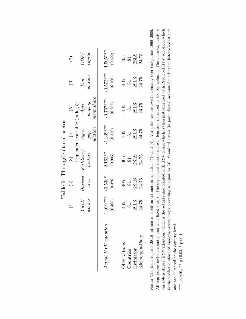
Table9:Theagriculturalsector

(1)

(2)

(3)

(4)

(5)

(6)

(7)


Yield/

Harvest

Fertilizer/

Agri.

Agri

Pop-

GDP/

worker

area

hectare

pop-

employ-

ulation

capita

ulation

mentshare

ActualHYVadoption

1.919***

-0.538*

2.162**

-1.339***

-0.767***

-0.572***1.505***

(0.468)

(0.326)

(0.905)

(0.338)

(0.252)

(0.186)

(0.422)

Observations

405

405

405

405

405

405

405

Countries

8181

8181

8181

81Estimator

2SLS

2SLS

2SLS

2SLS

2SLS

2SLS

2SLS

Kleibergen-Paap

24.75

24.75

24.75

24.75

24.75

24.75

24.75






***p<0.01,**p<0.05,*p<0.1

Table10:Demographiceffects

(1)

(2)

(3)

(4)

(5)

(6)

(7)

Dependentvariable:

(inlogs)

(inrates)

Life

Infant

AdultMortality

Fertility

Rateof

Pop-

Expec-mortality

female

male

rate

natural

ulation

tancy

increase

growth

ActualHYVadoption

0.134

-1.958***-1.689***-0.996***-1.524***-0.270***-0.274***

(0.0870)

(0.382)

(0.314)

(0.254)

(0.293)

(0.0636)

(0.0774)

Observations

420

381

420

420

420

420

420

Countries

8484

8484

8484

84Estimator

2SLS

2SLS

2SLS

2SLS

2SLS

2SLS

YES

Kleibergen-Paap

25.98

23.70

25.98

25.98

25.98

25.98

25.98






***p<0.01,**p<0.05,*p<0.1

Table11:TheimpactofHYVadoption,1960—2000

Averagedevelopingcountry

Developingworldtotal

HYVadoptionrateyear2000

27%

59%

HYVscontributiontoGDP/capitagrowth1960-2000

50pp

139pp

ActualGDP/capitagrowth1960-2000

57%

171%

HYVscontributiontopopulationgrowth1960-2000

-14pp

-27pp

Actualpopulationgrowth1960-2000

162%

129%

Notes:Calculationsbasedonourbaselineregressionresults.Seetextfordetails.

010

2030

40A

dopt

ion

rate

(per

cent

of c

ropl

and)

1960 1970 1980 1990 2000Y ear

Rice WheatBarley Cassav a

Figure 1: Adoption of high-yielding varieties of selected crops

Source: Gollin and Evenson (2003)

020

4060

80A

dopt

ion

rate

(per

cent

of c

ropl

and)

1960 1970 1980 1990 2000Y ear

India BrazilTurkey Nigeria

Figure 2: Adoption of high-yielding varieties in selected countries

Source: Gollin and Evenson (2003)

Figure 3: Agro-climatically attainable yields, selected crops

Panel A: sorghum

Panel B: wheat

Notes: The maps depict agro-climatically attainable yields for sorghum and wheat under the assumptions

of a high-input level and irrigation is used. Similar maps for the other eight crops we use in our analysis are

available in the Online Appendix. Source: FAO.

AGO

ARG

BEN

BFA

BGD

BOL

BRA

BWA

CAF

CHL

CHN

CMR

COG

COLCRI

CUB

DOM DZA

ECUEGY

ETH

GAB

GHA

GIN

GMB GNB

GTMHNDHTI

IDNIND

IRN

IRQ

JAM

KEN

KHM

LAOLBN

LBRLBY

LKA

MAR

MDG

MEX

MLI

MMR

MNG

MOZ

MRT MUS MWI

MYS

NAM

NER

NGA

NIC

NPL

PAK

PAN

PER

PHL

PRY

RWA

SAU

SDN

SEN

SLE

SLVSWZ

SYR

TCDTGO

THA

TUN

TUR

TZAUGA

URYVEN

VNM

YEMZAFZMB

ZWE

0.2

.4.6

.81

Actu

al H

YV a

dopt

ion

.05 .1 .15 .2 .25Predicted HYV adoption

Figure 4: Actual and predicted HYV adoption (in the year 2000)

Notes: This figure shows the scatter plot between actual HYV adoption and predicted HYV adoption in the

year 2000 (corresponding to the change between 1960 and 2000 as HYV adoption was zero for all countries

in 1960). The line is the fitted value between these two variables (coeff=2.91, p-val=0.00).

Figure 5: Partial Correlation Plots

AGO

ARGBENBFA

BGDBOL

BRA

BWA

CAF

CHL

CHN

CMRCOG

COLCRI

CUB

DOM

DZAECU

EGY

ETH

GAB GHA

GINGMB

GNBGTMHND

HTI

IDNIND

IRN

IRQ

JAMKEN KHMLAO

LBN

LBR

LBY

LKA

MAR

MDG

MEX

MLI

MMR

MNG

MOZ

MRT

MUS

MWI

MYS

NAM

NER

NGA

NIC

NPL

PAKPAN

PER

PHLPRY

RWA

SAU

SDNSEN

SLE

SLV

SWZSYR

TCDTGO

THA

TUNTUR

TZAUGA

URY

VEN

VNMYEM

ZAF

ZMB

ZWE

10

12

3C

hang

e in

log

GD

P/c

apita

0 .2 .4 .6Predicted change in HYV adoption

Panel A: income (i.e., log GDP/capita)

AGO

ARG

BEN

BFABGDBOLBRA

BWA

CAF

CHLCHN

CMR

COG

COL

CRI

CUB

DOM

DZAECU

EGYETHGAB GHA GIN

GMB

GNB

GTMHND

HTI

IDNIND

IRNIRQ

JAM

KEN

KHMLAO

LBN

LBR

LBY

LKA

MAR

MDGMEX

MLI

MMR

MNG

MOZMRT

MUS

MWI

MYS

NAMNER

NGANIC

NPL

PAK

PAN

PER PHLPRY

RWA

SAU

SDN

SEN

SLE

SLV

SWZ

SYR

TCD

TGO

THA TUNTUR

TZAUGA

URY

VEN

VNM

YEM

ZAF

ZMBZWE

0.5

11.

5C

hang

e in

log

popu

latio

n

0 .2 .4 .6Predicted change in HY V adoption

Panel B: Log Population

Notes: These figures show the partial correlation plots for long-differences specifications that only use the

years 1960 and 2000. The plots hold country and time-period fixed effects constant

two blades of grass: the impact of the green revolution

Documents