Using Intel® Processors for DSP Applications: Comparing the Performance of Freescale MPC8641D and Two Intel Core™2 Duo Processors

Mike DelvesN.A. Software Ltd

David TetleyGE Fanuc Intelligent Platforms

IntroductionThe high performance embedded DSP processor market has moved steadily over the past decade from one dominated by specialised fixed point processors towards those with recognisable similarities to the general­purpose processor market: DSP processors have provided floating point, substantial caches, and capable C/C++ compilers, as well as SIMD (Single Instruction Multiple Data)  features providing fast vector operations. The inclusion of SIMD features to general purpose processors has led to them replacing specialised DSPs in many high performance embedded applications (such as Radar, SAR, SIGINT and image processing). Indeed, probably the most widely used general purpose processor for DSP in the past five years is the PowerPC family, which was used for a long while in the Apple range of PCs. The G4 generation of the PowerPC has dominated the embedded high performance computing market for over 8 years.If the PowerPC can be accepted both in the general­purpose and the embedded DSP markets, what about other processor families? This question is motivated by the very fast rate of development of general­purpose silicon over the past four years: faster cycle times, larger caches, faster front side buses, lower­power variants, multi­core technology, vector instruction sets, and plans for more of everything well into the future, with development funded by the huge general­purpose market. Here, we look in particular at how well the current family of Intel® low power processors perform against the PowerPC.

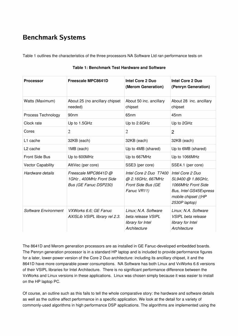
Benchmark Systems

Table 1 outlines the characteristics of the three processors NA Software Ltd ran performance tests on 

Table 1: Benchmark Test Hardware and Software

Processor Freescale MPC8641D Intel Core 2 Duo (Merom Generation)

Intel Core 2 Duo (Penryn Generation)

Watts (Maximum) About 25 (no ancillary chipset needed)

About 50 inc. ancillary chipset

About 28  inc. ancillary chipset

Process Technology 90nm 65nm 45nm

Clock rate Up to 1.5GHz Up to 2.6GHz Up to 2GHz

Cores 2 2 2L1 cache 32KB (each) 32KB (each) 32KB (each)

L2 cache 1MB (each) Up to 4MB (shared) Up to 6MB (shared)

Front Side Bus Up to 600MHz Up to 667MHz Up to 1066MHz

Vector Capability AltiVec (per core) SSE3 (per core) SSE4.1 (per core)

Hardware details Freescale MPC8641D @ 1GHz , 400MHz Front Side Bus (GE Fanuc DSP230)

Intel Core 2 Duo  T7400 @ 2.16GHz, 667MHz Front Side Bus (GE Fanuc VR11)

Intel Core 2 Duo SL9400 @ 1.86GHz,  1066MHz Front Side Bus, Intel GS45Express  mobile chipset ((HP 2530P laptop)

Software Environment VXWorks 6.6; GE Fanuc AXISLib VSIPL library rel 2.3.

Linux; N.A. Software beta release VSIPL library for Intel  Architecture

Linux; N.A. Software  VSIPL beta release  library for Intel  Architecture

The 8641D and Merom generation processors are as installed in GE Fanuc­developed embedded boards. The Penryn generation processor is in a standard HP laptop and is included to provide performance figures for a later, lower­power version of the Core 2 Duo architecture: including its ancillary chipset, it and the 8641D have more comparable power consumptions.  NA Software has both Linux and VxWorks 6.6 versions of their VSIPL libraries for Intel Architecture.  There is no significant performance difference between the VxWorks and Linux versions in these applications.  Linux was chosen simply because it was easier to install on the HP laptop PC.

Of course, an outline such as this fails to tell the whole comparative story: the hardware and software details as well as the outline affect performance in a specific application. We look at the detail for a variety of commonly­used algorithms in high performance DSP applications. The algorithms are implemented using the 

VSIPL API. VSIPL (Vector, Signal and Image Processing Library) is an industry standard API for DSP and vector math. Code written in VSIPL is not architecture dependent and portable to any platform supporting a VSIPL implementation. To minimise implementation issues, which can cloud the comparisons, timings are taken using optimised VSIPL libraries; even so, some implementation comments are made. 

For all the timings save where noted, the data is resident within the L2 cache on all three  processors. In all cases timings were taken with warm caches.   In most of the timings, only a single core on each device is utilised, to allow a direct core­for­core performance comparison.

1D FFTsFast Fourier Transforms are the cornerstone of many DSP applications, and DSP libraries put a great deal of effort into optimising them, typically with assembler modules for crucial parts, and with multi algorithms used depending on the size of the FFT. Everybody's favourite comparison benchmark is: how fast does a 1K complex in­place FFT run? Here's how fast:

Single 1D FFT

Table 2a complex to complex 1D in­place FFT: times in microsecondsTimes in italic indicate that the data requires a significant portion, or is too large to fit into cache

N 256 1K 4K 16K 64K 256K 512K8641D 2.4 10.0 71.4 414 2,264 22,990 73,998

T7400 1.4 6.5 37 202 1,033 5,220 17,587

SL9400  1.26  6.3  35.9 197 1,011 4,704 11,732

Figure 2a complex to complex 1D in­place FFT: MFLOPS = 5 N Log2(N) / (time for one FFT in microseconds)

Single precision complex FFT perfomance 

0100020003000400050006000700080009000

256 1024 4096 16384 65536 262144 524288

Vector size

MFL

OPS 8641D

IA MeromIA SL9400

Table 2b real to complex 1D FFT: times in microsecondsTimes in italic indicate that the data requires a significant portion, or is too large to fit into cache

N 256 1K 4K 16K 64K 256K 512K8641D 2.1 7.8 46.7 258 1,510 14,938 34,911

T7400 1.2 4.5 24 131 584 3,054 6,094

SL9400 1.0 3.8 21.6 121 535 2,895 5,654

Table 2c complex to real 1D  FFT: times in microsecondsTimes in italic indicate that the data requires a significant portion, or is too large to fit into cache

N 256 1K 4K 16K 64K 256K 512K8641D 2.1 7.9 45.2 235 1,434 14,417 34,174

T7400 1.2 4.6 24 132 582 2,979 6,195

SL9400 1.0 4.1 21.5 117 529 2,833 5,702

For modest lengths, up to 16K, the comparisons reflect primarily the relative processor cycle times.   For 

longer lengths, the major advantage shown by the Intel processors reflects also the  larger L2 cache  and higher front side bus speeds on these chips. Gratifyingly, the SL9400 gives slightly faster times than the higher power consumption T7400, and this result is generally reflected in the further times given below.

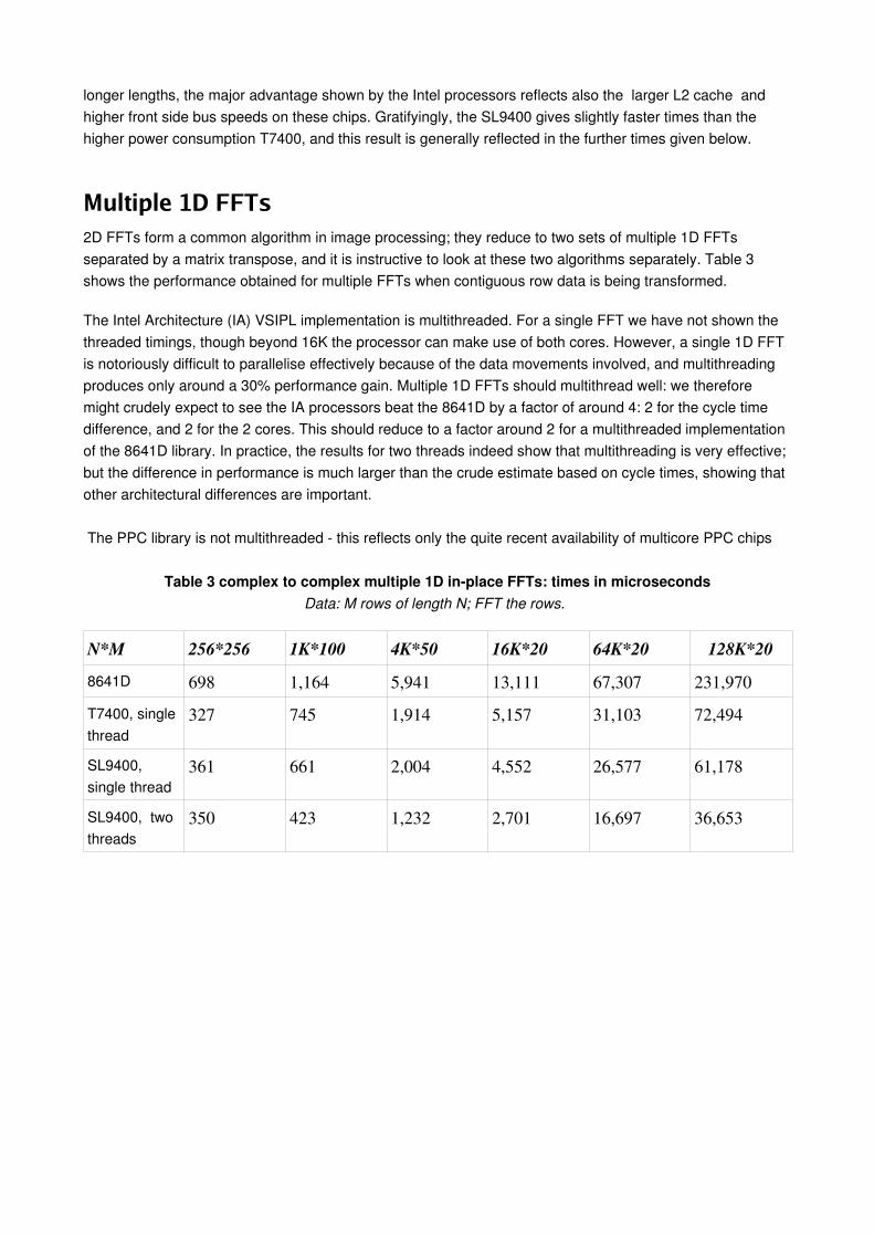
Multiple 1D FFTs2D FFTs form a common algorithm in image processing; they reduce to two sets of multiple 1D FFTs separated by a matrix transpose, and it is instructive to look at these two algorithms separately. Table 3 shows the performance obtained for multiple FFTs when contiguous row data is being transformed. 

The Intel Architecture (IA) VSIPL implementation is multithreaded. For a single FFT we have not shown the threaded timings, though beyond 16K the processor can make use of both cores. However, a single 1D FFT is notoriously difficult to parallelise effectively because of the data movements involved, and multithreading produces only around a 30% performance gain. Multiple 1D FFTs should multithread well: we therefore might crudely expect to see the IA processors beat the 8641D by a factor of around 4: 2 for the cycle time difference, and 2 for the 2 cores. This should reduce to a factor around 2 for a multithreaded implementation of the 8641D library. In practice, the results for two threads indeed show that multithreading is very effective; but the difference in performance is much larger than the crude estimate based on cycle times, showing that other architectural differences are important.

 The PPC library is not multithreaded ­ this reflects only the quite recent availability of multicore PPC chips

Table 3 complex to complex multiple 1D in­place FFTs: times in microsecondsData: M rows of length N; FFT the rows. 

N*M 256*256 1K*100 4K*50 16K*20 64K*20 128K*208641D 698 1,164 5,941 13,111 67,307 231,970

T7400, single thread

327 745 1,914 5,157 31,103 72,494

SL9400, single thread

361 661 2,004 4,552 26,577 61,178

SL9400,  two threads

350 423 1,232 2,701 16,697 36,653

Figure 3 complex to complex multiple 1D in­place FFTs: MFLOPS = 5 N Log2(N) / (time for one row FFT in microseconds)

Data: M rows of length N; FFT the rows. 

Single precision multiple FFT perfomance 

0

2000

4000

6000

8000

10000

12000

14000

256 x 256 1K x 100 4K x 50 16K x 20 64K x 20 128K x 20

Matrix size

MFL

OPS

8641D

IA T7400

IA SL9400

IA SL9400 ­two threads

Matrix Transpose

The results for matrix transpose calls for various N and M values are shown in Table 4a and 4B.  Matrix transpose is a memory­limited operation on these processors, and the faster front side bus, and larger cache size, give the Intel processors a major advantage for large matrices.

Table 4a real matrix transpose: times in microsecondsData: M rows of length N

N*M 256*256 1024*100 4K*50 16K*20 64K*208641D 166 190 2,700 5,591 32,728

T7400 74 97 435 472 20,784

SL9400 81 90 352 478 5,764

Table 4b complex matrix transpose: times in microsecondsData: M rows of length N 

N*M 256*256 1024*100 4K*50 16K*20 64K*208641D 877 902 6,744 11,859 65,511

T7400 178 362 768 2,384 43,064

SL9400 168 274 705 957 1,608

Vector Arithmetic

We distinguish two classes of vector operations:

1. Simple arithmetic, eg V3 := V1 + V2. For these operations it is possible to achieve near­optimal efficiency on long vectors.

2. Transcendental functions, eg V1 := sin(V2). For these operations, library routines go to a lot of trouble to provide better efficiency, with the use of assembler blocks being common. Quite small details of the processor instruction set can make substantial differences.

For both classes of routine, multithreading is very straightforward, indeed trivial, but again to avoid bias caused by the lack of multithreading in the 8641D library we report timings only on one core in each case.

Simple Vector ArithmeticTables 5a and 5b show typical comparisons for "easy" vector arithmetic routines. Note that italicized values in the following tables indicate that the data requires a significant proportion, or is too large to fit into a processors’ L2 cache.  Tables 5a and 5b makes it clear just how much difference large L2 caches make. The performance penalty is also shown graphically in Table 5b, where we have  expresses the timing results from Table 5a in terms of bandwidth.  For small N, the results roughly reflect the processors’ clock frequencies. As N increases, the better cache memory management on the Intel chip increases its lead over the PowerPC; and of course for large N the larger cache available with the Intel chips makes the battle very unequal indeed.  This is because the complex vector multiply calculation repeatedly works on the same area of memory—­for N=32K, nearly 1MB is required (32KB * sizeof(complex) * 3 vectors).  For N=128K, 3 MB of memory are required.  So the 8641D’s performance scales well at and below N=32K since a single core has 1MB of L2 cache.  But for N=64 and N=128 the data is 2 and 3x larger than its cache, resulting in a large number of cache misses and the memory latency penalty of having to access much slower main system memory.   Similar behaviour can be noted with the T7400.  The N=128K calculation requires three­fourths of the T7400’s L2 cache, so there will be a higher percentage of cache misses: its N=128K times are 4x its N=64K times, not merely 2x.  Conversely, the data only requires half of the Intel Core™2 Duo SL9400’s 6 MB cache: the N=128K times are almost precisely 2x its N=64K times. 

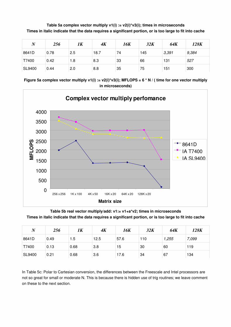
Table 5a complex vector multiply v1(i) := v2(i)*v3(i); times in microsecondsTimes in italic indicate that the data requires a significant portion, or is too large to fit into cache

N 256 1K 4K 16K 32K 64K 128K8641D 0.78 2.5 18.7 74 145 3,391 9,384

T7400 0.42 1.8 8.3 33 66 131 527

SL9400 0.44 2.0 8.8 35 75 151 300

Figure 5a complex vector multiply v1(i) := v2(i)*v3(i); MFLOPS = 6 * N / ( time for one vector multiply in microseconds)

Complex vector multiply perfomance 

0

500

1000

1500

2000

2500

3000

3500

4000

256 x 256 1K x 100 4K x 50 16K x 20 64K x 20 128K x 20

Matrix size

MFL

OPS 8641DIA T7400IA SL9400

Table 5b real vector multiply/add: v1:= v1+a*v2; times in microsecondsTimes in italic indicate that the data requires a significant portion, or is too large to fit into cache

N 256 1K 4K 16K 32K 64K 128K8641D 0.49 1.5 12.5 57.6 110 1,255 7,099

T7400 0.13 0.68 3.8 15 30 60 119

SL9400 0.21 0.68 3.6 17.6 34 67 134

In Table 5c: Polar to Cartesian conversion, the differences between the Freescale and Intel processors are not so great for small or moderate N. This is because there is hidden use of trig routines; we leave comment on these to the next section.

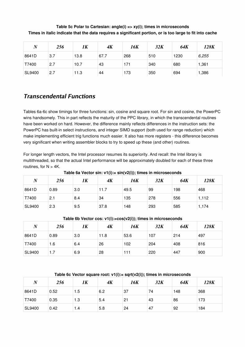
Table 5c Polar to Cartesian: angle(i) => xy(i); times in microsecondsTimes in italic indicate that the data requires a significant portion, or is too large to fit into cache

N 256 1K 4K 16K 32K 64K 128K8641D 3.7 13.8 67.7 268 510 1230 6,255

T7400 2.7 10.7 43 171 340 680 1,361

SL9400 2.7 11.3 44 173 350 694 1,386

Transcendental Functions

Tables 6a­6c show timings for three functions: sin, cosine and square root. For sin and cosine, the PowerPC wins handsomely. This in part reflects the maturity of the PPC library, in which the transcendental routines have been worked on hard. However, the difference mainly reflects differences in the instruction sets: the PowerPC has built­in select instructions, and integer SIMD support (both used for range reduction) which make implementing efficient trig functions much easier. It also has more registers ­ this difference becomes very significant when writing assembler blocks to try to speed up these (and other) routines.

For longer length vectors, the Intel processor resumes its superiority. And recall: the Intel library is multithreaded, so that the actual Intel performance will be approximately doubled for each of these three routines, for N > 4K.

Table 6a Vector sin: v1(i):= sin(v2(i)); times in microseconds

N 256 1K 4K 16K 32K 64K 128K8641D 0.89 3.0 11.7 49.5 99 198 468

T7400 2.1 8.4 34 135 278 556 1,112

SL9400 2.3 9.5 37.8 148 293 585 1,174

Table 6b Vector cos: v1(i):=cos(v2(i)); times in microseconds

N 256 1K 4K 16K 32K 64K 128K8641D 0.89 3.0 11.8 53.6 107 214 497

T7400 1.6 6.4 26 102 204 408 816

SL9400 1.7 6.9 28 111 220 447 900

Table 6c Vector square root: v1(i):= sqrt(v2(i)); times in microseconds

N 256 1K 4K 16K 32K 64K 128K8641D 0.52 1.5 6.2 37 74 148 368

T7400 0.35 1.3 5.4 21 43 86 173

SL9400 0.42 1.4 5.8 24 47 92 184

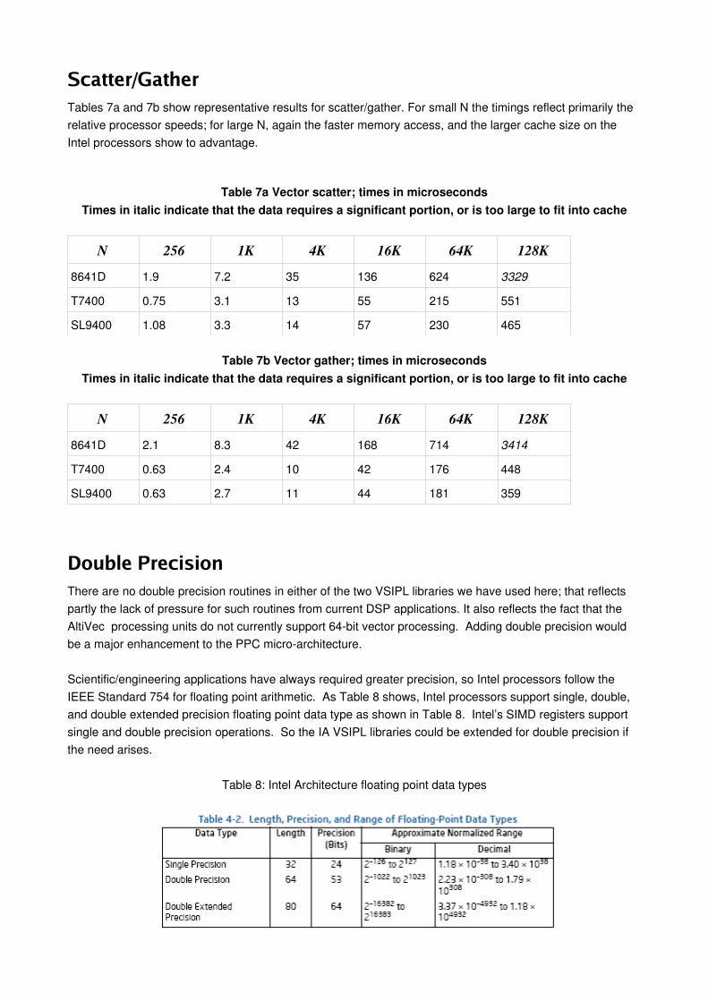
Scatter/GatherTables 7a and 7b show representative results for scatter/gather. For small N the timings reflect primarily the relative processor speeds; for large N, again the faster memory access, and the larger cache size on the Intel processors show to advantage.

Table 7a Vector scatter; times in microsecondsTimes in italic indicate that the data requires a significant portion, or is too large to fit into cache

N 256 1K 4K 16K 64K 128K8641D 1.9 7.2 35 136 624 3329

T7400 0.75 3.1 13 55 215 551

SL9400 1.08 3.3 14 57 230 465

Table 7b Vector gather; times in microsecondsTimes in italic indicate that the data requires a significant portion, or is too large to fit into cache

N 256 1K 4K 16K 64K 128K8641D 2.1 8.3 42 168 714 3414

T7400 0.63 2.4 10 42 176 448

SL9400 0.63 2.7 11 44 181 359

Double PrecisionThere are no double precision routines in either of the two VSIPL libraries we have used here; that reflects partly the lack of pressure for such routines from current DSP applications. It also reflects the fact that the AltiVec  processing units do not currently support 64­bit vector processing.  Adding double precision would be a major enhancement to the PPC micro­architecture.

Scientific/engineering applications have always required greater precision, so Intel processors follow the IEEE Standard 754 for floating point arithmetic.  As Table 8 shows, Intel processors support single, double, and double extended precision floating point data type as shown in Table 8.  Intel’s SIMD registers support single and double precision operations.  So the IA VSIPL libraries could be extended for double precision if the need arises.

Table 8: Intel Architecture floating point data types

A Look at the Intel Future

Intel Streaming SIMD Extensions (SSE)Intel Architecture (IA) Streaming SIMD Extension (SSE) instructions began with the Pentium® II and Pentium with MMX technology processor families.  There have been six subsequent expansions which have added more operations for both integer and floating point data elements.  Currently shipping Intel processors (as of March 2009) implement all previous MMX/SSE instructions as well as 47 new SSE4.1 operations.  Intel Core i7 processors add support for 7 additional SSE4.2 instructions.

Intel processors originally issued one SIMD operation per clock.  But the instruction scheduler in the Intel Core™ microarchitecture, first introduced in 2006, can issue four instructions simultaneously across five logical units – two of which are floating point Arithmetic Logical Units (ALUs).  (The other three logical units include a Load, a Store, and an ALU which handles integer arithmetic or SSE/FP moves and branches.). This means that each processor core can execute up to eight (8) single­precision floating point instructions per clock cycle – 4 on each FP ALU.  

Of course these additional FP ALUs and expanded SSE instructions require balanced improvements in memory and I/O subsystem bandwidth and latency if the processors are to reach their full potential.  Intel has recently begun shipping next generation “Nehalem” family processors.  These Intel Core™ i7 processors implement integrated memory controllers which exhibit greater memory bandwidth, and lower latency than Penryn family processors.  They also support the latest generation, higher speed DDR3 memory technologies.  In addition many of the newest processors and chipsets support PCI Express* Generation 2 I/O rates, which are 2X faster than generation 1 rates.  

Intel® Advanced Vector Extensions (Intel® AVX): New SIMD Instructions and MicroarchitectureIntel has announced a significant enhancement for floating point SIMD processing which will debut in the “Sandy Bridge” processor generation (2010­2011).  Intel® AVX increases the width of SIMD vectors and register sets from 128­bits to 256­bits.  Intel® AVX also includes new three­ and four­operand (non­destructive) instructions, 256­bit primitives for data permutes, etc.  

More than two hundred legacy Intel® SSEx instructions will be upgraded to use the new operand instructions and flexible memory alignment enhancements.  In addition, about 100 legacy 128­bit Intel® SSEx instructions will be promoted to process 256­bit vector data.   

The wider Intel® AVX SIMD implementation will double the theoretical GFLOPS of Intel processors.  

    

Multicore Extensions

Our experience with multithreading on multicore architectures convinces us that multithreading a single DSP application provides a relatively straightforward and very effective route to increased DSP performance. This is especially the case if maximum use is made of multithreaded libraries: then the bulk of the application can be maintained on a single thread and code changes are minimised.Intel’s current processor roadmap offers 1, 2, 4, and 6­core processors.   This means that a highly 

parallelized, multi­threaded DSP application can theoretically take advantage of up to 48 single­precision FP instructions per processor cycle, assuming a server with 4 processors, each of which has 6 cores (2 FP ops per cycle per 24 cores).

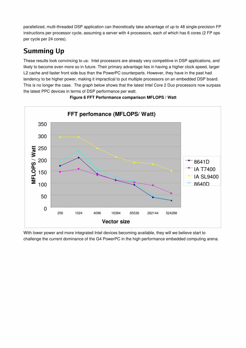
Summing UpThese results look convincing to us:  Intel processors are already very competitive in DSP applications, and likely to become even more so in future. Their primary advantage lies in having a higher clock speed, larger L2 cache and faster front side bus than the PowerPC counterparts. However, they have in the past had tendency to be higher power, making it impractical to put multiple processors on an embedded DSP board. This is no longer the case.  The graph below shows that the latest Intel Core 2 Duo processors now surpass the latest PPC devices in terms of DSP performance per watt.

Figure 6 FFT Performance comparison MFLOPS / Watt

 FFT perfomance (MFLOPS/ Watt) 

0

50

100

150

200

250

300

350

256 1024 4096 16384 65536 262144 524288

Vector size

MFL

OPS

 / W

att

8641DIA T7400IA SL94008640D

With lower power and more integrated Intel devices becoming available, they will we believe start to challenge the current dominance of the G4 PowerPC in the high performance embedded computing arena.