variable selection and model choice in survival models with
TRANSCRIPT
Variable Selection and Model Choice in SurvivalModels with Time-Varying Effects
Boosting Survival Models
Benjamin Hofner 1
Department of Medical Informatics, Biometry and Epidemiology (IMBE)
Friedrich-Alexander-Universitat Erlangen-Nurnberg
joint work with Thomas Kneib and Torsten Hothorn
Department of Statistics
Ludwig-Maximilians-Universitat Munchen
useR! 2008

Introduction Technical Preparations CoxflexBoost Summary / Outlook References
Introduction
Cox PH model:
λi (t) = λ(t, xi ) = λ0(t) exp(x′iβ)
with
λi (t) hazard rate of observation i [i = 1, . . . , n]
λ0(t) baseline hazard rate
xi vector of covariates for observation i [i = 1, . . . , n]
β vector of regression coefficients
Problem: restrictive model, not allowing for
non-proportional hazards (e.g., time-varying effects)
non-linear effects

Introduction Technical Preparations CoxflexBoost Summary / Outlook References
Additive Hazard Regression
Generalisation: Additive Hazard Regression(Kneib & Fahrmeir, 2007)
λi (t) = exp(ηi (t))
with
ηi (t) =J∑
j=1
fj(xi(t)),
generic representation of covariate effects fj(xi )
a) linear effects: fj(xi (t)) = flinear(xi ) = xiβb) smooth effects: fj(xi (t)) = fsmooth(xi )c) time-varying effects: fj(xi (t)) = fsmooth(t) · xi
where xi ∈ xi (t).
Note:
c) includes log-baseline for xi ≡ 1
Introduction Technical Preparations CoxflexBoost Summary / Outlook References
P-Splines
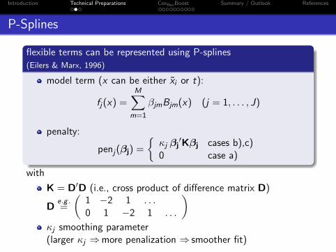
flexible terms can be represented using P-splines(Eilers & Marx, 1996)
model term (x can be either xi or t):
fj(x) =M∑
m=1
βjmBjm(x) (j = 1, . . . , J)
penalty:
penj(βj) =
{κj βj
′Kβj cases b),c)0 case a)
with
K = D′D (i.e., cross product of difference matrix D)
De.g .=
(1 −2 1 . . .0 1 −2 1 . . .
)κj smoothing parameter(larger κj ⇒more penalization ⇒ smoother fit)

Introduction Technical Preparations CoxflexBoost Summary / Outlook References
Inference
Penalized Likelihood Criterion: (NB: this is the full log-likelihood)
Lpen(β) =n∑
i=1
[δiηi (ti )−
∫ ti
0exp(ηi (t)) dt
]−
J∑j=0
penj(βj)
Ti true survival time
Ci censoring time
ti = min(Ti ,Ci ) observed survival time (right censoring)
δi = 1(Ti ≤ Ci ) indicator for non-censoring
Problem:
Estimation and in particular model choice

Introduction Technical Preparations CoxflexBoost Summary / Outlook References
CoxflexBoost
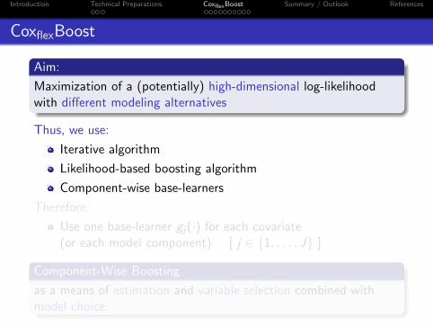
Aim:
Maximization of a (potentially) high-dimensional log-likelihoodwith different modeling alternatives
Thus, we use:
Iterative algorithm
Likelihood-based boosting algorithm
Component-wise base-learners
Therefore:
Use one base-learner gj(·) for each covariate(or each model component) [ j ∈ {1, . . . , J} ]
Component-Wise Boosting
as a means of estimation and variable selection combined withmodel choice.
Introduction Technical Preparations CoxflexBoost Summary / Outlook References
CoxflexBoost
Aim:
Maximization of a (potentially) high-dimensional log-likelihoodwith different modeling alternatives
Thus, we use:
Iterative algorithm
Likelihood-based boosting algorithm
Component-wise base-learners
Therefore:
Use one base-learner gj(·) for each covariate(or each model component) [ j ∈ {1, . . . , J} ]
Component-Wise Boosting
as a means of estimation and variable selection combined withmodel choice.
Introduction Technical Preparations CoxflexBoost Summary / Outlook References
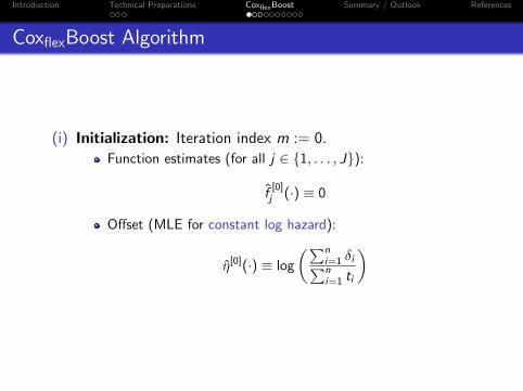
CoxflexBoost Algorithm
(i) Initialization: Iteration index m := 0.
Function estimates (for all j ∈ {1, . . . , J}):
f[0]j (·) ≡ 0
Offset (MLE for constant log hazard):
η[0](·) ≡ log
(∑ni=1 δi∑ni=1 ti
)
Introduction Technical Preparations CoxflexBoost Summary / Outlook References
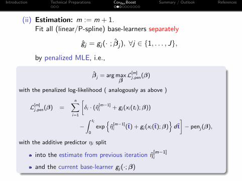
(ii) Estimation: m := m + 1.Fit all (linear/P-spline) base-learners separately
gj = gj(· ; βj), ∀j ∈ {1, . . . , J},
by penalized MLE, i.e.,
βj = arg maxβL[m]
j,pen(β)
with the penalized log-likelihood ( analogously as above )
L[m]j,pen(β) =
n∑i=1
[δi · (η[m−1]
i + gj(xi (ti ); β))
−∫ ti
0
exp{η
[m−1]i (t) + gj(xi (t); β)
}d t
]− penj(β),
with the additive predictor ηi split
into the estimate from previous iteration η[m−1]i
and the current base-learner gj(·; β)

Introduction Technical Preparations CoxflexBoost Summary / Outlook References
(iii) Selection: Choose base-learner gj∗ with
j∗ = arg maxj∈{1,...,J}
L[m]j ,unpen(βj)
(iv) Update:Function estimates (for all j ∈ {1, . . . , J}):
f[m]j =
{f
[m−1]j + ν · gj j = j∗
f[m−1]j j 6= j∗
Additive predictor (= fit):
η[m] = η[m−1] + ν · gj∗
with step-length ν ∈ (0, 1] (here: ν = 0.1)
(v) Stopping rule: Continue iterating steps (ii) to (iv) untilm = mstop
Introduction Technical Preparations CoxflexBoost Summary / Outlook References
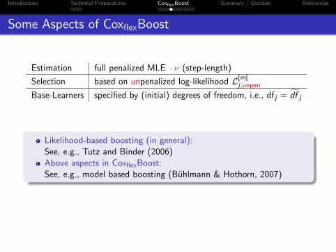
Some Aspects of CoxflexBoost
Estimation full penalized MLE · ν (step-length)
Selection based on unpenalized log-likelihood L[m]j ,unpen
Base-Learners specified by (initial) degrees of freedom, i.e., df j = df j
Likelihood-based boosting (in general):See, e.g., Tutz and Binder (2006)Above aspects in CoxflexBoost:See, e.g., model based boosting (Buhlmann & Hothorn, 2007)

Introduction Technical Preparations CoxflexBoost Summary / Outlook References
Degrees of Freedom
Specifying df more intuitive thanspecifying smoothing parameter κ
Comparable to other modeling components, e.g., linear effects
Problem: Not constant over the (boosting) iterations
But simulation studies showed: No big deviation from the
initial df j = df j
0 200 400 600 800
0.0
0.2
0.4
0.6
0.8
1.0
bbs((x3))
boosting iteration m
df((m
))
Estimated degrees of freedom tracedover the boosting steps for the flexi-ble base-learners of x3 (in 200 repli-cates) and initially specified degreesof freedom (dashed line).
Introduction Technical Preparations CoxflexBoost Summary / Outlook References
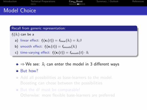
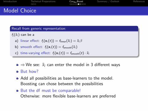
Model Choice
Recall from generic representation:
fj(xi ) can be a
a) linear effect: fj(xi (t)) = flinear(xi ) = xiβ
b) smooth effect: fj(xi (t)) = fsmooth(xi )
c) time-varying effect: fj(xi (t)) = fsmooth(t) · xi
⇒We see: xi can enter the model in 3 different ways
But how?
Add all possibilities as base-learners to the model.Boosting can chose between the possibilities
But the df must be comparable!Otherwise: more flexible base-learners are preferred
Introduction Technical Preparations CoxflexBoost Summary / Outlook References
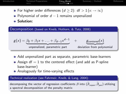
For higher order differences (d ≥ 2): df > 1 (κ→∞)
Polynomial of order d − 1 remains unpenalized
Solution:
Decomposition (based on Kneib, Hothorn, & Tutz, 2008)
g(x) = β0 + β1x + . . .+ βd−1xd−1︸ ︷︷ ︸
unpenalized, parametric part
+ gcentered(x)︸ ︷︷ ︸deviation from polynomial
Add unpenalized part as separate, parametric base-learners
Assign df = 1 to the centered effect (and add as P-splinebase-learner)Analogously for time-varying effects
Technical realization (see Fahrmeir, Kneib, & Lang, 2004):
decomposing the vector of regression coefficients β into (βunpen, βpen) utilizinga spectral decomposition of the penalty matrix
Introduction Technical Preparations CoxflexBoost Summary / Outlook References
Early Stopping
1 Run the algorithm mstop-times (previously defined).2 Determine new mstop,opt ≤ mstop:
... based on out-of-bag sample (with simulations easy to use)
... based on information criterion, e.g., AIC
⇒Prevents algorithm to stop in a local maximum(of the log-likelihood)
⇒Early stopping prevents overfitting
Introduction Technical Preparations CoxflexBoost Summary / Outlook References
Variable Selection and Model Choice
... is achieved by
selection of base-learner (in step (iii) of CoxflexBoost), i.e.,component-wise boostingand
early stopping
Simulation-Results (in Short)
Good variable selection strategy
Good model choice strategy if only linear and smooth effectsare used
Selection bias in favor of time-varying base-learners (ifpresent) ⇒ standardizing time could be a solution
Estimates are better if model choice is performed

Introduction Technical Preparations CoxflexBoost Summary / Outlook References
Computational Aspects
CoxflexBoost is implemented using R
Crucial computation: Integral in L[m]j ,pen(β):∫ ti
0exp
{η
[m−1]i (t) + gj(xi (t); β)
}d t
time consuming
very often evaluated (maximization of L[m]j,pen(β))
R-function integrate() slow in this context⇒ (specialized) vectorized trapezoid integration implemented⇒≈ 100 times quicker
Efficient storage of matrices can reduce computational burden⇒ recycling of results
Introduction Technical Preparations CoxflexBoost Summary / Outlook References
Summary & Outlook
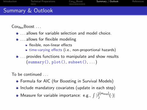
CoxflexBoost . . .
. . . allows for variable selection and model choice.
. . . allows for flexible modeling
flexible, non-linear effectstime-varying effects (i.e., non-proportional hazards)
. . . provides functions to manipulate and show results(summary(), plot(), subset(), . . . )
To be continued . . .
Formula for AIC (for Boosting in Survival Models)
Include mandatory covariates (update in each step)
Measure for variable importance: e.g.,∫|f [mstop ]
j (·)|
Introduction Technical Preparations CoxflexBoost Summary / Outlook References
Summary & Outlook
CoxflexBoost . . .
. . . allows for variable selection and model choice.
. . . allows for flexible modeling
flexible, non-linear effectstime-varying effects (i.e., non-proportional hazards)
. . . provides functions to manipulate and show results(summary(), plot(), subset(), . . . )
To be continued . . .
Formula for AIC (for Boosting in Survival Models)
Include mandatory covariates (update in each step)
Measure for variable importance: e.g.,∫|f [mstop ]
j (·)|
Introduction Technical Preparations CoxflexBoost Summary / Outlook References
Literature
Buhlmann, P., & Hothorn, T. (2007). Boosting algorithms:Regularization, prediction and model fitting. Statistical Science,22(4), 477-505.
Eilers, P. H. C., & Marx, B. D. (1996). Flexible smoothing withB-splines and penalties. Statistical Science, 11(2), 89–121.
Fahrmeir, L., Kneib, T., & Lang, S. (2004). Penalized structuredadditive regression: A Bayesian perspective. Statistica Sinica,14, 731–761.
Kneib, T., & Fahrmeir, L. (2007). A mixed model approach forgeoadditive hazard regression. Scand. J. Statist., 34, 207–228.
Kneib, T., Hothorn, T., & Tutz, G. (2008). Variable selection andmodel choice in geoadditive regression. Biometrics (accepted).
Tutz, G., & Binder, H. (2006). Generalized additive modelling withimplicit variable selection by likelihood-based boosting.Biometrics, 62, 961–971.

l with model choice
−1.0 −0.5 0.0 0.5 1.0
−0.
8−
0.6
−0.
4−
0.2
0.0
0.2
0.4
x1
log(
haza
rd r
ate)
l without model choice
−1.0 −0.5 0.0 0.5 1.0
−0.
8−
0.6
−0.
4−
0.2
0.0
0.2
0.4
x1
log(
haza
rd r
ate)
−2 −1 0 1 2
−3
−2
−1
01
23
x4
log(
haza
rd r
ate)
−3 −2 −1 0 1 2
−2
02
x4
log(
haza
rd r
ate)

0 2 4 6 8 10
−6
−4
−2
02
time
log(
haza
rd r
ate)
0 2 4 6 8 10
−6
−4
−2
02
time
log(
haza
rd r
ate)